P. Tkalich, K.Y.H. Gin, and E.S. Chan Physical Oceanography Research Laboratory Tropical Marine Science Institute The National University of Singapore.

P. Tkalich , K.Y.H. Gin, and E.S. Chan

Physical Oceanography Research Laboratory

Tropical Marine Science Institute

The National University of Singapore

TMSITMSI

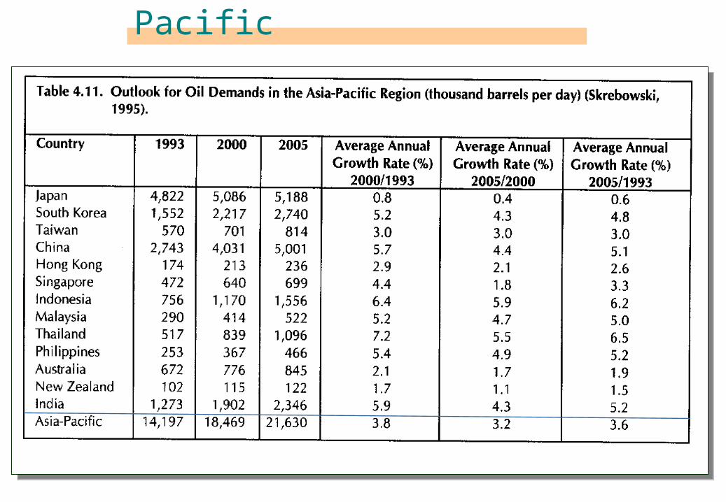
Oil Demand in Asia-Pacific

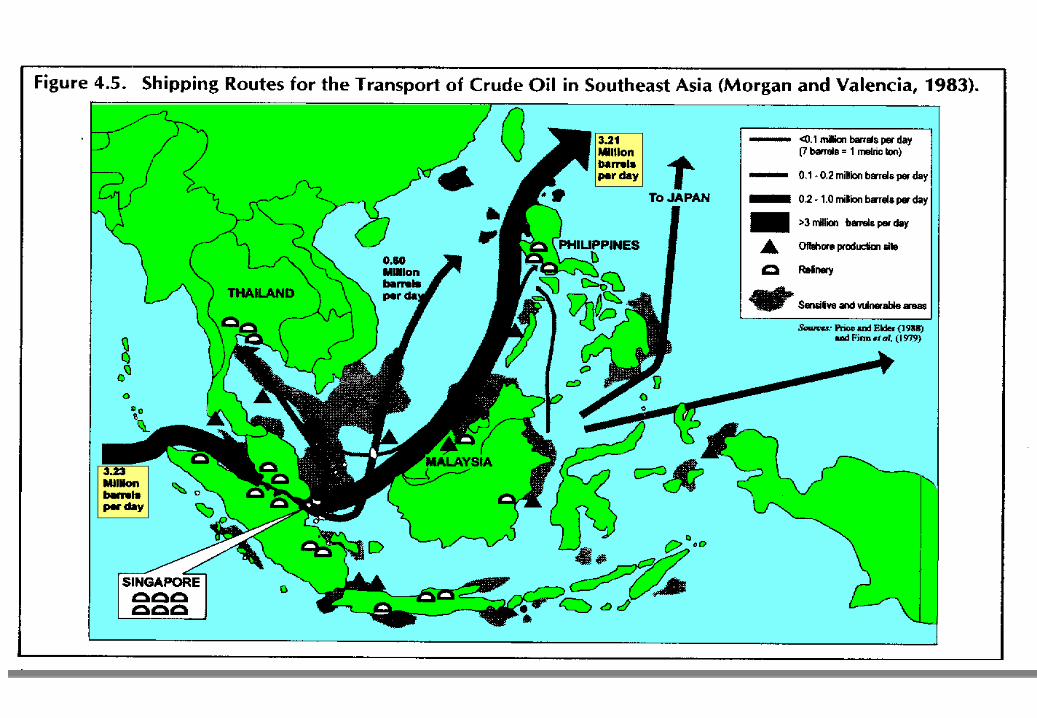
Global Movement of Oil in 199

5 oil refineries in Singapore waters have total capacity over 1 mil. barrels per day.(second largest refinery area in the world, after Houston, Texas)

5 oil refineries in Singapore waters have total capacity over 1 mil. barrels per day.(second largest refinery area in the world, after Houston, Texas)

Malacca&Singapore Straits

Major Oil Spills

SlNo.

Date Name of Spill Type of oil Volume(tons)

Economiccost ($)

1 March, 1989 Exxon Valdez Crude 34061 2 October, 1997 Evoikos Marine Fuel 28000 3 February, 1970 Arrow Bunker C Fuel 16000 4 January, 1993 Braer Crude

Heavy Fuel85000 500

5 January, 1989 Bahia Paraiso Diesel FuelArctic

600

6 August, 1989 Mersey Crude 150

Money spent by Exxon Corporation subsequent to EVOS (in millions of dollars) ------------------------------------------------------ Immediate Costs (1989, 19990)

Cleanup $2,000 Fisherman 300

Out-of-Court Settlement (1991-2001) Damage assesment 214 Habitat protection 375 Administrative costs 35 Research, monitoring

and general restoration 180 Restoration reserve 108 Accumulated interest

less Court fees 12------------------------------------ TOTAL $3,224

Civil Trial (1995) Compensation to fishermen $287 Punitive compensation (under appeal) 5000

Money spent by Exxon Corporation subsequent to EVOS (in millions of dollars) ------------------------------------------------------ Immediate Costs (1989, 19990)

Cleanup $2,000 Fisherman 300

Out-of-Court Settlement (1991-2001) Damage assesment 214 Habitat protection 375 Administrative costs 35 Research, monitoring

and general restoration 180 Restoration reserve 108 Accumulated interest

less Court fees 12------------------------------------ TOTAL $3,224

Civil Trial (1995) Compensation to fishermen $287 Punitive compensation (under appeal) 5000

Evoikos spill

Evoikos spill

Evoikos spill

Oil Properties

Properties \ Oil typeCrude oil(Kuwait)

No. 2Fuel oil

Bunker CFuel oil

API gravity (20oC) 31.4 31.6 7.3Viscosity at 77oF(cS) 2600 3.1 2800Paraffins (wt %) 34.0 61.8 21.1Naphthenes (wt %) 22.7 0.0 0.0Aromatics (wt %) 21.9 38.2 34.2Others (wt %) 21.4 0.0 44.7Sulfur & Nitrogen (wt %) 2.58 0.34 2.4Heavy metal (ppm) 35.7 2.0 162.0

tarballs

evaporation

oxidationphotolysis

emulsificationdissolution

hydrolysisbiodegradation

foodweb

sedimentation

Oil FateOil Fate

wind

gravitationinertiaviscousinterf.tension

Oil Kinetics

12

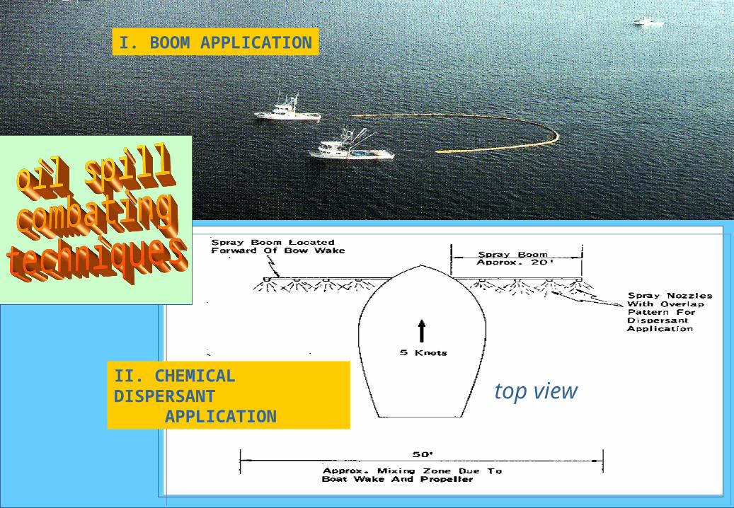
I. BOOM APPLICATION

top view II. CHEMICAL DISPERSANT APPLICATION

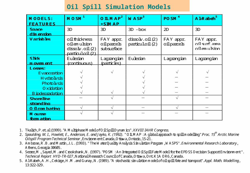
MODELS:FEATURES

MOSM1 OILMAP2

+SIMAPWASP3 POSM4 Al-Rabeh5

Spacedimension

3D 3D 3D - box 2D 3D

Variables oil thicknessoil emulsiondissolv. oil (2)particul.oil (2)

FAY appr.oil parcelssubsurface

dissolv. oil (2)particul.oil (2)

FAY appr.oil parcels

FAY appr.oil surf. areaoil emulsion

Slickmovement

Eulerian(continuous)

Lagrangian(particles)

Eulerian Lagrangian Lagrangian

Losses:Evaporation Hydrolysis Photolysis Oxidation

Biodegradation Shorelinestranding

Oil combating Mousseformation

1. Tkalich, P. et. al (1999). "A Multiphase Model of Oil Spill Dynamics". XXVIII IAHR Congress.2. Spaulding, M. I., Howlett, E., Anderson, E. and Jayko, K. (1992). " OILMAP : A global approach to spill modelling".Proc. 15th Arctic Marine

Oilspill Program Technical Seminar, Environment Canada, Ottawa, Ontario, 15-21.3. Ambrose, R. B. and Martin, J. L. (1993). " The Water Quality Analysis Simulation Program, WASP5". Environmental Research Laboratory,

Athens, Georgia 30605.4. Serrer, M., Sayed, M. and Crookshank, N. (1997). "POSM : An Integrated Oil Spill Fate Model for the EPDSS Decision Support Environment ".

Technical Report HYD-TR-027, National Research Council of Canada, Ottawa, Ont. K1A OR6, Canada. 5. Al-Rabeh, A. H., Cekirge, H. M. and Gunay, N. (1989). "A stochastic simulation model of oil spill fate and transport". Appl. Math. Modelling,

13:322-329.

Oil Spill Simulation Models

14

Fay (1971) considered three phases of oil slick spreading.

a. Gravity-inertia phase : D = K1 (gV)1/4 t1/2

b. Gravity-viscous : D = K2 (gV2/1/2)1/6 t1/4

c. Surface tension-viscous : D = K3 [/(1/2)]1/2 t3/4

Where D= axi-symmetrical spreading diameter; V = total volume of oil spill;

= kinematic viscosity of water, = interfacial tension,

= 1 - o/, o = Density of oil, = Density of water, g = acceleration due to

gravity,

t = time and K1, K2 & K3 = Constant.

Oil Slick DynamicsOil Slick Dynamics

Navier-Stokes equations

(gravity - viscosity regime)

.)(

,)(

,0

oooyo

oooxo

oo

fhuvvky

hgh

fhvuukx

hgh

y

hv

x

hu

t

h

u o , v o = a v e r a g e d v e lo c i t y o f t h e o i l s l i c k p a r t i c l e s ; /)( o ; = d e n s i ty o f w a te r ;

o = d e n s i ty o f o i l ; g = a c c e l e r a t i o n d u e t o g r a v i t y ; u , v a n d w = f l u id v e lo c i ty i n x - , y -a n d z - d i r e c t i o n , r e s p e c t i v e ly ; U , V = w in d v e lo c i ty i n x - a n d y - d i r e c t i o n ,r e s p e c t i v e ly ; VkUk yx 03.0/ ,03.0/ = s h e a r s t r e s s e s d u e t o w in d ; f = C o r io l i s

a c c e l e r a t i o n ; k = w a t e r - o i l f r i c t i o n c o e f f i c i e n t

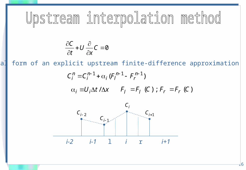
16

0

Cx

Ut

C

)( 111 nr

nli

ni

ni FFCC

xtU ii /

General form of an explicit upstream finite-difference approximation

iC

1iC2iC 1iC

i-2 i-1 l i r i+1

)( );( CFFCFF rrll

17

HIGH - ORDER ADVECTION APPROXIMATION

USING POLYNOMIAL INTERPOLATION

1niP

niC

1niC1

1

niC

niC 1

space

time

x ix1ix

/)( 1 xxx ii

1 ni

ni PC

1nt

nt

/ tUx i

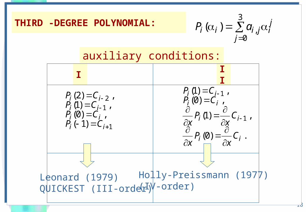
18

THIRD -DEGREE POLYNOMIAL:

3

0,)(

j

jijiii aP

1

12

)1(, )0(

, )1(, )2(

iiiiiiii

CPCPCPCP

. )0(

, )1(

, )0(, )1(

1

1

ii

ii

iiii

Cx

Px

Cx

Px

CPCP

Leonard (1979)QUICKEST (III-order)

auxiliary conditions:

I II

Holly-Preissmann (1977)(IV-order)

19

6/)1(6/)235(6/)32( 212

211

211

ni

ni

ni

nl CCCF

)( 111 nr

nli

ni

ni FFCC

iC

1iC2iC 1iC

i-2 i-1 l i r i+1

III-order QUICKEST (Leonard, 1979)

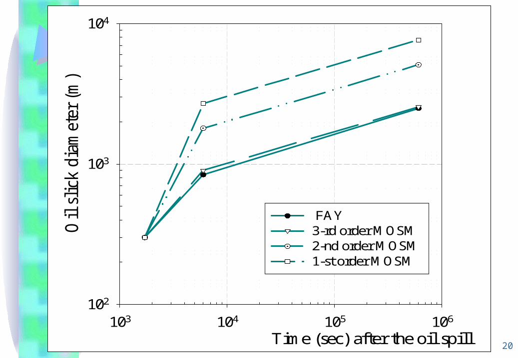
20Time (sec) after the oil spill

103 104 105 106

Oil

sli

ck d

iam

eter

(m

)

102

103

104

FAY 3-rd order MOSM 2-nd order MOSM 1-st order MOSM

Oil Transfer at Media Interfaces oil slick oil-in-water emulsion

(due to wind - waves breaking)

h

zh

wave breaking

oil buoyancy

h=kw(1+Sg)H

h=0.2 g-1 kw(1+Sg)U2

Sg = 0 /w

U

.

,

o

o

esee

ee

se

Cz

Kh

dt

dC

CKh

dt

dh

.

,

o

o

esee

ee

se

Cz

Kh

dt

dC

CKh

dt

dh

Ce = Concentration of oil emulsion in the water column

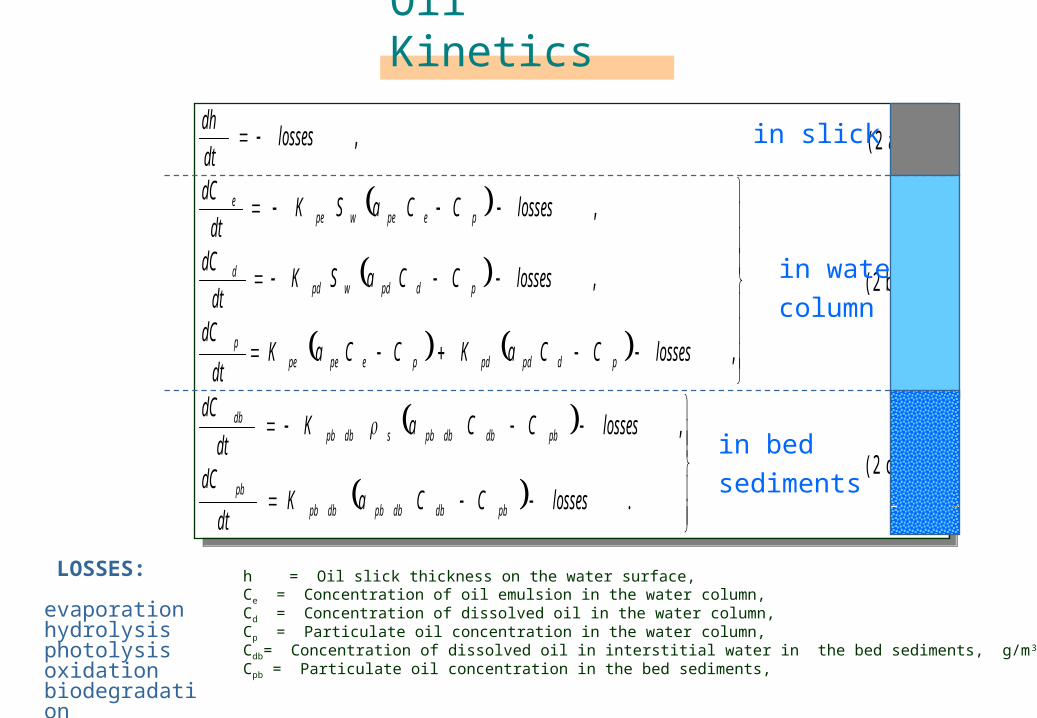
Oil Kinetics

, lossesdt

dh ( 2 a )

,

,

,

lossesCCaKCCaKdt

dC

lossesCCaSKdt

dC

lossesCCaSKdt

dC

pdpdpdpepepep

pdpdwpdd

pepewpee

( 2 b )

.

,

lossesCCaKdt

dC

lossesCCaKdt

dC

pbdbdbpbdbpbpb

pbdbdbpbsdbpbdb

( 2 c )

, lossesdt

dh ( 2 a )

,

,

,

lossesCCaKCCaKdt

dC

lossesCCaSKdt

dC

lossesCCaSKdt

dC

pdpdpdpepepep

pdpdwpdd

pepewpee

( 2 b )

.

,

lossesCCaKdt

dC

lossesCCaKdt

dC

pbdbdbpbdbpbpb

pbdbdbpbsdbpbdb

( 2 c )

h = Oil slick thickness on the water surface, mCe = Concentration of oil emulsion in the water column, g/m3

Cd = Concentration of dissolved oil in the water column, g/m3

Cp = Particulate oil concentration in the water column, g/kgCdb= Concentration of dissolved oil in interstitial water in the bed sediments, g/m3

Cpb = Particulate oil concentration in the bed sediments, g/kg

in slick

in water

column

in bed

sediments

LOSSES:

evaporationhydrolysisphotolysisoxidationbiodegradation

RC

EC

EC

E

z

WwC

y

vC

x

uC

t

C

zyx

z

z y

y x

x

RC

EC

EC

E

z

WwC

y

vC

x

uC

t

C

zyx

z

z y

y x

x

Transport of the oil phases in the water column

Here pdennCC ,,

= concentration of n-th oil phase;

pdennRR ,,

= physical-chemical kinetics;

Ex , Ey and Ez = turbulent eddy coefficients;

pdennWW ,,

= settling velocity of the oil phases.

Ce = Concentration of oil emulsion in the water column, Cd = Concentration of dissolved oil in the water column, Cp = Particulate oil concentration in the water column,

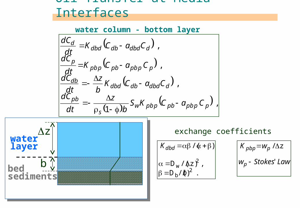
Oil Transfer at Media Interfaces water column - bottom layer

, 1

,

,

,

pppbpbppbws

pb

dddbdbddbdb

pppbpbppbp

dddbdbddbd

CaCKSb

z

dt

dC

CaCKb

z

dt

dC

CaCKdt

dC

CaCKdt

dC

b

water layer

bed sediments

z

. )/(D , z)/(D

)/(

2b

2w

b

K ddb

LawStokesw

wK

p

ppbp

'

z/

exchange coefficients

Model Parameters Parameters description Notation Value UnitsDissolution rate Ksd 5.695x10-1 s-1

Mass transfer rate (slick to emulsion) Kse 7.30x10-6 s-1

Susp.sediment/Wat.column distr.coeff apd 1.760 m3/kgBed sedim./Pore water distr. coefficient apb db 0.500 m3/kgSusp.sediment/Emulsion distr. coeff. ape 2.910x10-3 m3/kgPartit. coeff. “pore water” – “water col.” adb d 1 ---Partit.coeff. “bed sedim” – “susp. sed” apb p 1 ---Sorption rate at water column Kpd 4.724x10-5 s-1

Sorption rate at bed sediment Kpb dp 2.931x10-9 s-1

Sorption rate Kpe 1.670x10-2 s-1

Sediment/water exchange rate Kdb d 7.353x10-8 s-1

Sedimentation rate Kpb p 3.150x10-6 s-1

Volatilization rate (oil slick) Ksv 4.884x10-3 s-1

Volatilization rate (emulsion) Kev 2.723x10-7 s-1

Volatilization rate (dissolved) Kdv 2.723x10-6 s-1

Photolysis rate Kp 5.530x10-6 s-1

Oxidation rate Ko 3.875x10-6 s-1

Biodegradation rate (water column) Ktw 6.543x10-7 s-1

Biodegradation rate (bed sediment) Ktb 1.227x10-7 s-1

Comparison with data

27

Comparison with data

Oil Spill at Open Sea Channel 2-D test case

60 m

500 km

U=7 m/soil 28,000 T

u=1 m/sL=

surface fence

29

Distance in km

0 100 200 300 400 500

Oil

sli

ck

th

ick

ness (

h),

m

0.0000

0.0002

0.0003

0.0005

0.0006

0.0d0.5d

1.0d

1.5d

2.0d2.5d 3.0d

3.5d 4.0d

Initial oil slick thickness, ho = 0.006 m

2D simulation. Oil slick thickness

Distance in km

0 100 200 300 400 500

Cd

b in

g/m3

0

48x10-9

96x10-9

144x10-9

1.5d

2.0d

2.5d

3.0d

3.5d

4.0d

1.0d

Dissolved oil concentration in pore water of bed sediments

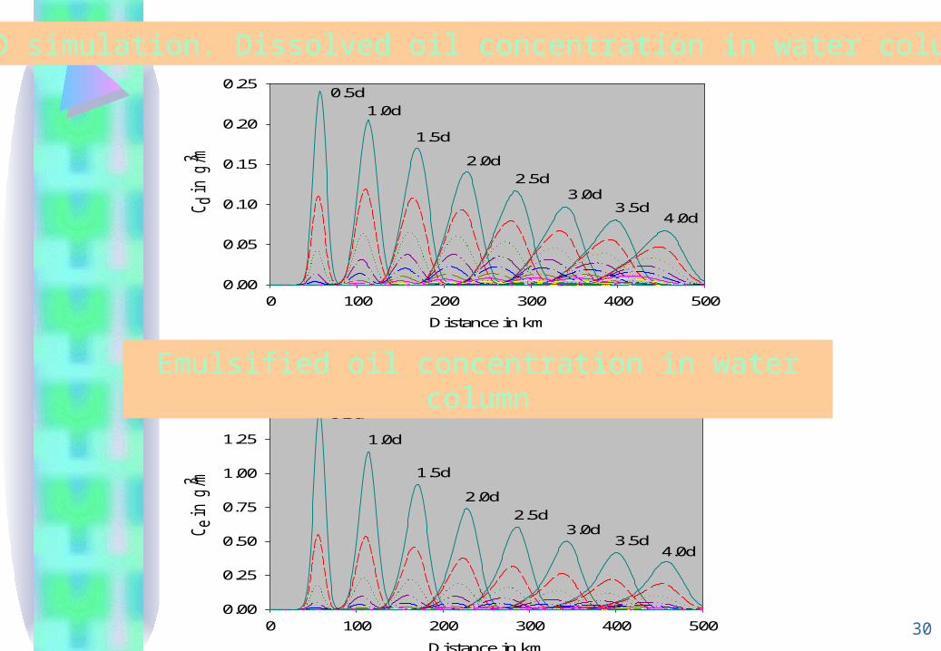
30

Distance in km

0 100 200 300 400 500

Cd

in g

/m3

0.00

0.05

0.10

0.15

0.20

0.250.5d

1.0d

1.5d

2.0d

2.5d3.0d

3.5d4.0d

2D simulation. Dissolved oil concentration in water column

Distance in km

0 100 200 300 400 500

Ce

in g

/m3

0.00

0.25

0.50

0.75

1.00

1.25

1.500.5d

1.0d

1.5d

2.0d

2.5d3.0d

3.5d4.0d

Emulsified oil concentration in water column

31

Oil Mass Balance

Time (days) after oil spill

0 1 2 3 4

Am

ou

nt

of

oil

(%

)

0

20

40

60

80

100

Atmosphere Water Surface Water Column

32

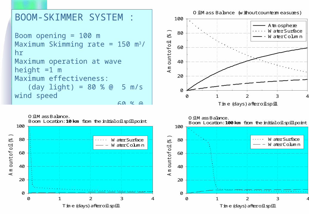
BOOM-SKIMMER SYSTEM :

Boom opening = 100 mMaximum Skimming rate = 150 m3/ hrMaximum operation at wave height =1 mMaximum effectiveness: (day light) = 80 % @ 5 m/s wind speed 60 % @ 10 m/s (night) = 50 % of day light values.

Oil Mass Balance (without countermeasures)

Time (days) a fte r oil spill

0 1 2 3 4

Am

ou

nt

of

oil

(%

)

0

20

40

60

80

100

Atmosphere Water Surface Water Column

Time (days) after oil spill

0 1 2 3 4

Am

ou

nt

of

oil

(%

)

0

20

40

60

80

100

Water Surface Water Column

Oil Mass Balance.Boom Location: 10 km from the initial oil spill point

Oil Mass Balance.Boom Location: 100 km from the initial oil spill point

Time (days) after oil spill

0 1 2 3 4

Am

ount

of

oil

(%

)

0

20

40

60

80

100

Water Surface Water Column

33

DISPERSANT APPLICATION :

Dispersant : Arcochem D-609Oil : Dispersant Ratio = 143 : 1Maximum dispersant effectiveness = 80 %Lethal concentration (LC50) for Zooplankton (Mysidopsis bahia) = 29 ppm (96 hrs exposure period)Spray width = 50 ft

Oil Mass Balance.Dispersant used 1 hour after the oil spill.

Time (days) after oil spill

0 1 2 3 4

Am

ou

nt

of

oil

(%

)

0

20

40

60

80

100

Atmosphere Water Surface Water Column

Oil Mass Balance. Dispersant used 1 day after the oil spill.

Time (days) after oil spill

0 1 2 3 4

Am

ou

nt

of

oil

(%

)

0

20

40

60

80

100

Atmosphere Water Surface Water Column

Oil Mass Balance (without countermeasures)

Time (days) after oil spill

0 1 2 3 4

Am

ount

of

oil

(%

)

0

20

40

60

80

100

Atmosphere Water Surface Water Column

0 2 0 ,0 0 0 4 0 ,0 0 0 6 0 ,0 0 0 8 0 ,0 0 0 1 0 0 ,0 0 0

m

0

2 0 ,0 0 0

4 0 ,0 0 0

m

S IN G A P O R E

Jo h o r

- 0

2 0

4 0

6 0

8 0

1 0 0

1 2 0

0 2 0 ,0 0 0 4 0 ,0 0 0 6 0 ,0 0 0 8 0 ,0 0 0 1 0 0 ,0 0 0

m

0

2 0 ,0 0 0

4 0 ,0 0 0

m

S IN G A P O R E

Jo h o r

- 0

2 0

4 0

6 0

8 0

1 0 0

1 2 0

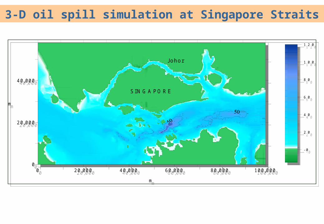
3-D oil spill simulation at Singapore Straits

Surface currents at one instant of tidal cycle for the south-west monsoon

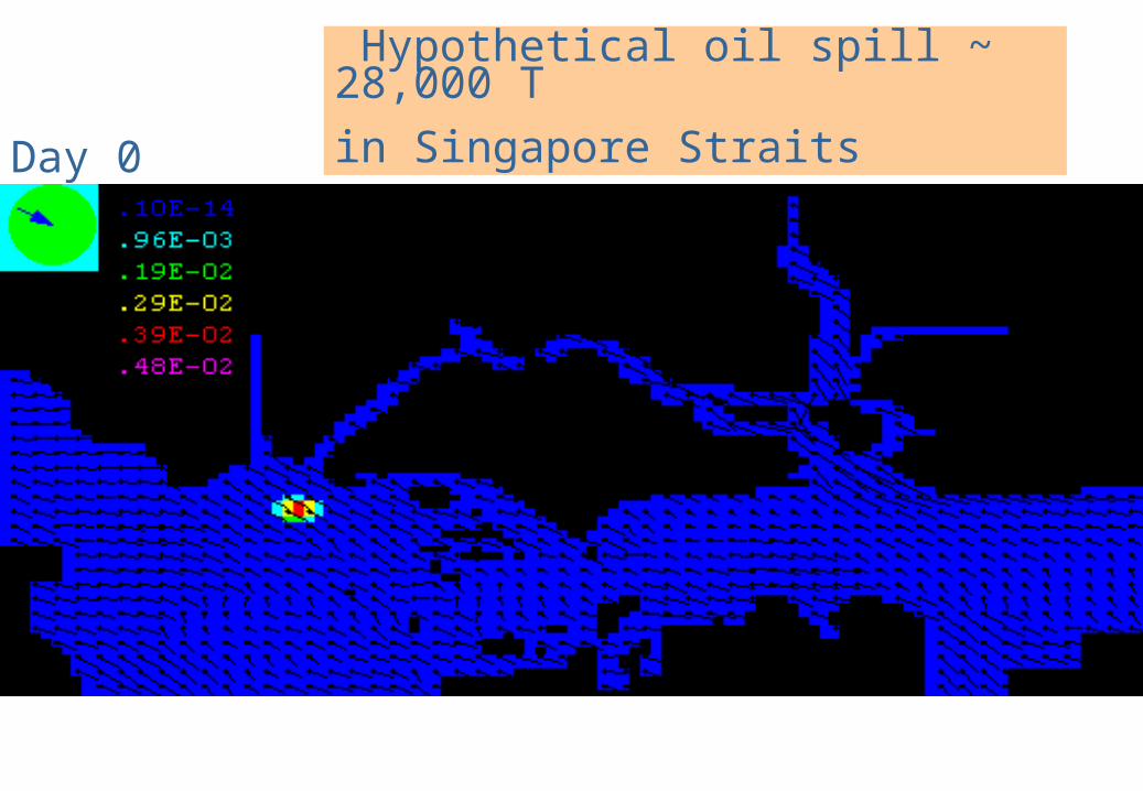
Day 0

Hypothetical oil spill ~ 28,000 T

in Singapore Straits

Day 0.5

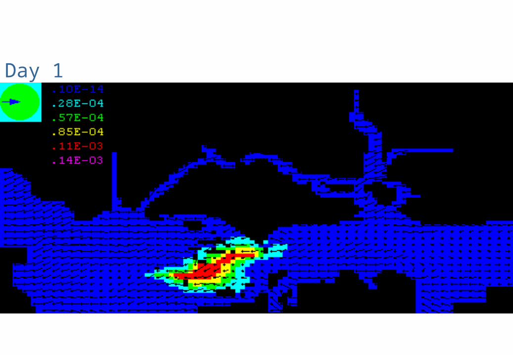
Day 1

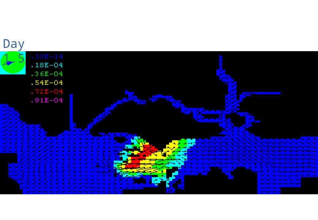
Day 1.5

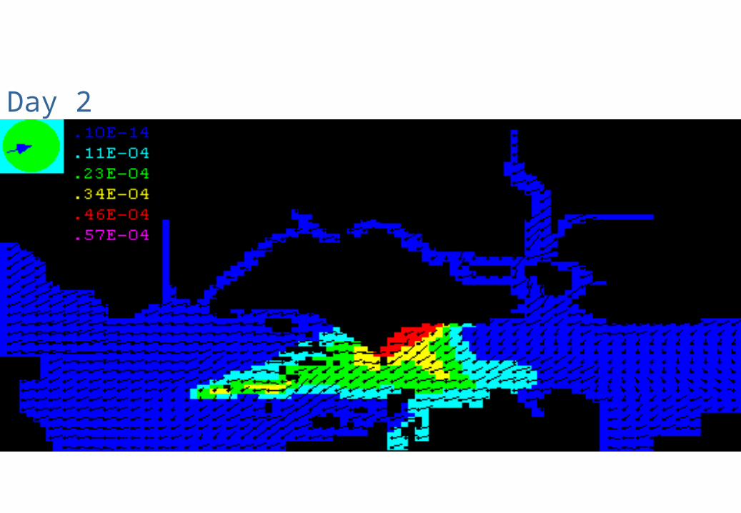
Day 2

Day 2.5

Day 3

Conclusions

The three-dimensional multiphase oil spill model is developed to simulate the consequences of accidental oil releases in the Singapore Straits.

The model is updated with a high-order numerical scheme for accurate simulation of the oil slick dynamics.

MOSM is powered with the oil combating techniques evaluation sub-module. Test simulations show a good agreement with empirical data.

The three-dimensional multiphase oil spill model is developed to simulate the consequences of accidental oil releases in the Singapore Straits.

The model is updated with a high-order numerical scheme for accurate simulation of the oil slick dynamics.

MOSM is powered with the oil combating techniques evaluation sub-module. Test simulations show a good agreement with empirical data.