OXYGEN DIFFUSION THROUGH TITANIUM AND OTHER HCP METALS BY HENRY WU DISSERTATION Submitted in partial fulfillment of the requirements for the degree of Doctor of Philosophy in Materials Science and Engineering in the Graduate College of the University of Illinois at Urbana-Champaign, 2013 Urbana, Illinois Doctoral Committee: Associate Professor Dallas R. Trinkle, Director of Research Professor Robert S. Averback Professor Pascal Bellon Assistant Professor Elif Ertekin

Welcome message from author
This document is posted to help you gain knowledge. Please leave a comment to let me know what you think about it! Share it to your friends and learn new things together.
Transcript

OXYGEN DIFFUSION THROUGH TITANIUM AND OTHER HCP METALS
BY
HENRY WU
DISSERTATION
Submitted in partial fulfillment of the requirementsfor the degree of Doctor of Philosophy in Materials Science and Engineering
in the Graduate College of theUniversity of Illinois at Urbana-Champaign, 2013
Urbana, Illinois
Doctoral Committee:
Associate Professor Dallas R. Trinkle, Director of ResearchProfessor Robert S. AverbackProfessor Pascal BellonAssistant Professor Elif Ertekin
ABSTRACT
Titanium alloys, due to their high tensile strength, low density, and excellent corrosion re-
sistance, have great potential in aerospace and medical implant applications. However, Ti
alloy properties are very sensitive to oxygen content and readily oxidizes at high temper-
atures. Ab initio density functional theory calculations are utilized to study the atomistic
mechanism of oxygen diffusion in titanium as well as the effect of substitutional solutes on
oxygen diffusivity. Oxygen is found to reside at three interstitials in α-titanium, the octa-
hedral, hexahedral, and crowdion sites. Transitions between these interstitial sites form a
complex diffusion network in which almost all pathways contribute to diffusion. The interac-
tion energy between oxygen and 45 substitutional solutes are calculated and used to predict
how each solute changes oxygen diffusion through titanium. Additionally, the energetics
and diffusion pathways for oxygen in 14 other hexagonal closed-packed (HCP) elements are
studied, revealing that in most HCP systems the ground-state for oxygen is not the large
octahedral site.
ii

Dedicated to my family.
iii

ACKNOWLEDGMENTS
First and foremost, I would like to thank Dallas Trinkle for his mentorship and guidance. It
was only with his help that I am able to develop the scientific mindset that I have today. I
will always be indebted to you Dallas. Thank you for everything.
I want to give thanks to my thesis committee members: Professors Bob Averback, Pascal
Bellon and Elif Ertekin for their helpful suggestions and support. Special thanks to Dr. Don
Shih from Boeing for helpful discussions relating to my research.
I want to thank all past and current graduate students in the Trinkle group: Joseph Yasi,
Maryam Ghazisaeidi, Min Yu, Pinchao Zhang, Emily Schiavone, Zebo Li, Ah-Young Song,
Abhinav Jain, Ravi Agarwal, and Anne Marie Tan. I also want to thank past and current
post-doctoral researchers: Hadley Lawler, Venkateswara Rao Manga, Thomas Garnier, Bora
Lee, and Mike Fellinger. I also wish to acknowledge the undergraduate students I have
worked with and whom have assisted in my research: Chanda Lowrance, Pandu Wisesa, and
Arvind Srikanth.
Special thanks to Andrew Signor and John Weaver for their research collaboration on the
study of Cu/Ag(111) island diffusion. It is unfortunate that the results from this surface
diffusion study will not be included within this thesis.
Finally I want to thank everyone I have met at the University of Illinois. You have all made
iv
my time here an interesting and valuable experience.
Financial support for this research was provided by NSF/CMMI CAREER award 0846624
and The Boeing Company. I gratefully acknowledge use of the Turing and Taub clusters
maintained and operated by the Computational Science and Engineering Program at the
University of Illinois; as well as the Texas Advanced Computing Center (TACC) at the
University of Texas as Austin.
v

TABLE OF CONTENTS
List of Tables . . . . . . . . . . . . . . . . . . . . . . . . . . . . . . . . . . . . . . . . viii
List of Figures . . . . . . . . . . . . . . . . . . . . . . . . . . . . . . . . . . . . . . . ix
List of Abbreviations . . . . . . . . . . . . . . . . . . . . . . . . . . . . . . . . . . . . xi
List of Symbols . . . . . . . . . . . . . . . . . . . . . . . . . . . . . . . . . . . . . . . xii
Chapter 1 Introduction and Background . . . . . . . . . . . . . . . . . . . . . . . . 11.1 Oxygen in HCP . . . . . . . . . . . . . . . . . . . . . . . . . . . . . . . . . . 11.2 Oxygen in Titanium . . . . . . . . . . . . . . . . . . . . . . . . . . . . . . . 21.3 Research Scope . . . . . . . . . . . . . . . . . . . . . . . . . . . . . . . . . . 51.4 Computational Approach . . . . . . . . . . . . . . . . . . . . . . . . . . . . . 61.5 Outline . . . . . . . . . . . . . . . . . . . . . . . . . . . . . . . . . . . . . . . 7
Chapter 2 Oxygen Diffusion in Titanium . . . . . . . . . . . . . . . . . . . . . . . . 82.1 Computational Method . . . . . . . . . . . . . . . . . . . . . . . . . . . . . . 82.2 Oxygen Interstitial Sites in Titanium . . . . . . . . . . . . . . . . . . . . . . 112.3 Oxygen Transition Pathways in Titanium . . . . . . . . . . . . . . . . . . . . 14
2.3.1 Treatment of Oxygen and Titanium in Density-Functional Theory:USPP and PAW . . . . . . . . . . . . . . . . . . . . . . . . . . . . . 16
2.4 Oxygen Diffusion Through Pure Titanium . . . . . . . . . . . . . . . . . . . 172.4.1 Full Diffusion Equations . . . . . . . . . . . . . . . . . . . . . . . . . 172.4.2 Diffusivity Through Subnetworks . . . . . . . . . . . . . . . . . . . . 24
2.5 Summary . . . . . . . . . . . . . . . . . . . . . . . . . . . . . . . . . . . . . 26
Chapter 3 Effect of Solutes on Oxygen Diffusion Through Titanium . . . . . . . . . 273.1 Computational Method . . . . . . . . . . . . . . . . . . . . . . . . . . . . . . 27
3.1.1 Pseudopotential Valence For Computed Solutes . . . . . . . . . . . . 273.1.2 Kinetically Resolved Activation Barrier Approximation . . . . . . . . 28
3.2 Solute-Oxygen Interaction Energy . . . . . . . . . . . . . . . . . . . . . . . . 303.3 Numerical Diffusion Model Predictions . . . . . . . . . . . . . . . . . . . . . 353.4 Accelerated Diffusion . . . . . . . . . . . . . . . . . . . . . . . . . . . . . . . 413.5 Non-Dilute Solute Concentrations . . . . . . . . . . . . . . . . . . . . . . . . 43
3.5.1 Multiple Solute Types . . . . . . . . . . . . . . . . . . . . . . . . . . 44
vi

3.5.2 Solute Effect on Oxygen Diffusion in Ti-6Al-4V . . . . . . . . . . . . 453.6 Approximation Errors in the Diffusion Model . . . . . . . . . . . . . . . . . . 473.7 Summary . . . . . . . . . . . . . . . . . . . . . . . . . . . . . . . . . . . . . 50
Chapter 4 Oxygen Diffusion in HCP Metals . . . . . . . . . . . . . . . . . . . . . . 524.1 Computational Methods . . . . . . . . . . . . . . . . . . . . . . . . . . . . . 524.2 Oxygen Interstitial Sites in HCP Lattices . . . . . . . . . . . . . . . . . . . . 534.3 Oxygen Transition Pathways in HCP Lattices . . . . . . . . . . . . . . . . . 544.4 Oxygen Diffusion Through HCP Metals . . . . . . . . . . . . . . . . . . . . . 584.5 Trends in Oxygen Energetics in HCP Metals . . . . . . . . . . . . . . . . . . 624.6 Summary . . . . . . . . . . . . . . . . . . . . . . . . . . . . . . . . . . . . . 67
Chapter 5 Conclusion and Future Work . . . . . . . . . . . . . . . . . . . . . . . . . 695.1 Summary of Results . . . . . . . . . . . . . . . . . . . . . . . . . . . . . . . 695.2 Future Work . . . . . . . . . . . . . . . . . . . . . . . . . . . . . . . . . . . . 70
References . . . . . . . . . . . . . . . . . . . . . . . . . . . . . . . . . . . . . . . . . . 71
vii

LIST OF TABLES
2.1 Transition pathways, prefactors ν, and energy barriers E for oxygen diffusionin α-titanium, between octahedral (o), hexahedral (h), and crowdion (c) sites. 16
2.2 USPP and PAW site energies and transition barriers for oxygen in titanium. 17
3.1 Substitutional solutes and their pseudopotential valence configurations. . . . 273.2 Table of oxygen-solute interaction energies for different oxygen and solute
configurations. . . . . . . . . . . . . . . . . . . . . . . . . . . . . . . . . . . . 323.3 Table of the change in diffusivity for oxygen in Ti-X at 900K. . . . . . . . . 383.4 Table of the solute activation barriers to oxygen diffusion in Ti-X at 900K. . 393.5 Comparison between KRA and DFT transition barriers for oxygen in titanium. 483.6 Table of oxygen-solute interaction energies for octahedral neighbors beyond
the first nearest neighbor. . . . . . . . . . . . . . . . . . . . . . . . . . . . . 48
4.1 PAW pseudopotential valence configurations for the 15 HCP elements andoxygen. . . . . . . . . . . . . . . . . . . . . . . . . . . . . . . . . . . . . . . 53
4.2 Analytical diffusion equations for individual transition networks from Figure 4.2. 564.3 Debye temperature, Debye frequency, and estimated attempt frequency for
HCP elements. . . . . . . . . . . . . . . . . . . . . . . . . . . . . . . . . . . 60
viii

LIST OF FIGURES
1.1 HCP crystal structure of Ti. . . . . . . . . . . . . . . . . . . . . . . . . . . . 21.2 Effect of oxygen content on the mechanical properties of titanium. . . . . . . 31.3 Binary phase diagram for Ti-O. . . . . . . . . . . . . . . . . . . . . . . . . . 4
2.1 Attempt frequency calculation with Ti force constants. . . . . . . . . . . . . 102.2 Wyckoff positions and relative energies for oxygen interstitial sites in α-titanium. 122.3 Oxygen interstitial sites and oxygen diffusion pathways in α-titanium. . . . . 142.4 Fractional contributions to oxygen diffusion through titanium from individual
diffusion networks in the basal and c-axis directions. . . . . . . . . . . . . . . 212.5 C-axis vs. basal diffusion ratios from our diffusion model and experimentally
measured diffusion anisotropy values. . . . . . . . . . . . . . . . . . . . . . . 222.6 Oxygen diffusion in titanium, by-passing the crowdion site. . . . . . . . . . . 232.7 Approximate analytical diffusion equations for oxygen in titanium diffusion
sub-networks. . . . . . . . . . . . . . . . . . . . . . . . . . . . . . . . . . . . 242.8 Analytical results and experimental data of oxygen diffusivity in α-titanium. 25
3.1 Schematic diagram of KRA approximation for transition between site A and B. 283.2 Extracting the change in basal diffusivity of oxygen with Al and Co solutes
at 900K. . . . . . . . . . . . . . . . . . . . . . . . . . . . . . . . . . . . . . . 303.3 Neighboring solute positions for each of the three oxygen interstitial sites in
titanium. . . . . . . . . . . . . . . . . . . . . . . . . . . . . . . . . . . . . . . 303.4 Schematic configurations used to calculate oxygen-solute interaction energy. . 313.5 Plot of oxygen-solute interaction energies for different oxygen interstitials and
solute configurations. . . . . . . . . . . . . . . . . . . . . . . . . . . . . . . . 333.6 Predicted diffusivity changes for oxygen in titanium at 900K for individual
solute neighbor interactions. . . . . . . . . . . . . . . . . . . . . . . . . . . . 353.7 Change in diffusivity of oxygen in Ti-X at 900K. . . . . . . . . . . . . . . . . 373.8 Solute activation barriers to oxygen diffusion in Ti-X at 900K. . . . . . . . . 393.9 1D diffusion system with a single type of interstitial site under the influence
of repulsive and attractive solutes. . . . . . . . . . . . . . . . . . . . . . . . . 423.10 1D diffusion system with two types of interstitial sites under the influence of
a solute that is attractive for the metastable interstitial. . . . . . . . . . . . . 423.11 Effect of non-dilute solute concentrations on oxygen diffusivity at 900K. . . . 433.12 Effect of multiple non-dilute solutes on oxygen diffusivity in Ti at 900K. . . 45
ix
3.13 Effect of non-dilute solute concentrations on oxygen diffusivity in Ti-6Al-4Vat 900K. . . . . . . . . . . . . . . . . . . . . . . . . . . . . . . . . . . . . . . 46
3.14 Solute interaction energy beyond the first nearest neighbor of oxygen in theoctahedral site. . . . . . . . . . . . . . . . . . . . . . . . . . . . . . . . . . . 49
4.1 Wyckoff positions and unit cell locations for oxygen interstitial sites in HCPsystems. . . . . . . . . . . . . . . . . . . . . . . . . . . . . . . . . . . . . . . 54
4.2 Connectivity network for transitions between interstitial sites in the HCP lattice. 554.3 Oxygen interstitial site energies and diffusion barriers in all 15 HCP elements. 574.4 Comparison between our DFT predicted and experimentally measured oxygen
diffusivity in Ti, Hf, Zr, Y, and Sc. . . . . . . . . . . . . . . . . . . . . . . . 614.5 DFT oxygen diffusion predictions for the remaining 10 HCP elements. . . . . 614.6 Correlation with respect to oxygen energetics between the 15 HCP elements. 634.7 Comparison of oxygen interstitial energetics for Ti, Zr, and Hf. . . . . . . . . 644.8 Comparison of oxygen interstitial energetics for Sc and Y. . . . . . . . . . . 654.9 Comparison of oxygen interstitial energetics for Tc, Ru, Re, and Os. . . . . . 654.10 Comparison between c-axis and basal diffusion for Os, Re, Ru, and Tc. . . . 664.11 Comparison of oxygen interstitial energetics for Zn and Cd. . . . . . . . . . . 664.12 Comparison of oxygen interstitial energetics for Be, Mg, Co, and Tl. . . . . . 67
x
LIST OF ABBREVIATIONS
DFT Density Functional Theory.
GGA Generalized Gradient Approximation.
HCP Hexagonal Close-Packed.
HTST Harmonic Transition State Theory.
KRA Kinetically Resolved Activation Barrier.
LDA Local Density Approximation.
MSD Multi-State Diffusion
NEB Nudged Elastic Band.
PAW Projector Augmented Wave.
PBE Perdew-Burke-Ernzerhof GGA Exchange-Correlation.
PW91 Perdew-Wang 91 GGA Exchange-Correlation.
TST Transition State Theory.
USPP Ultrasoft Pseudopotential.
xi

LIST OF SYMBOLS
a HCP ~a lattice constant.
c HCP ~c lattice constant.
λ Transition rate.
ν Attempt frequency prefactor.
kB Boltzmann’s constant.
T Temperature.
Dbasal Basal diffusion constant.
Dc-axis C-axis diffusion constant.
xi→j Normalized reaction coordinate for transition saddle point from site i to site j.
εsi Solute interaction energy at the interstitial site i from the solute atom at the latticesite s.
α Infinite dilute solute effect on oxygen diffusivity.
xii

CHAPTER 1
INTRODUCTION ANDBACKGROUND
1.1 Oxygen in HCP
The presence of light element impurities determine many material properties, including
phase transition kinetics[1], precipitates in semiconductors[2], and hydrogen embrittlement
in steels[3]. Oxygen content in particular need to be carefully controlled to balance the
increase in hardness with decrease in ductility for titanium allooys[4]. While many studies
have experimentally measured the diffusion of oxygen through various metal alloy systems,
there is a lack of a fundamental atomistic understanding of how oxygen diffuse through many
basic metal systems.
The hexagonal close-packed (HCP) crystal structure is space group[5] 194, P63/mmc;
and is the low temperature phase for many elements. Even in this simple lattice it is difficult
to experimentally determine the atomistic mechanisms for interstitial diffusion. Contributing
to this difficulty is the short residence time of interstitial species at meta-stable configura-
tions. However even the exact ground-state configuration can be hard to confirm since low
interstitial solubility limits the use of X-ray diffraction.
Many elements of industrial interests possess the HCP crystal structure. Titanium alloys
are of particular interest for their high strength and low density. However, beating out even
titanium is magnesium; at only 2/3 the density of Al, Mg is the lightest structural metal. Its
lower cost also makes it much more appealing to the transportation industry. An examination
of interstitial behavior in Mg may provide insight into solving its poor formability and
poor corrosion resistance. Zirconium alloys are used as nuclear reactor cladding due to
1
zirconium’s low neutron absorption cross section. However Zr alloys suffer from similar
oxidation problems as Ti alloys as well as hydrogen embrittlement. Light element interstitial
energetics in zirconium are therefore critical in understanding and preventing these problems.
1.2 Oxygen in Titanium
First discovered in 1791 by William Gregor, Titanium is named after the Titans of Greek
mythology. However, it was only in 1910 that pure metallic titanium was extracted by
Matthew A. Hunter. Titanium is polymorphic; with the low temperature hexagonal closed-
packed (HCP) α-phase transforming at 1155K into the body-centered cubic (BCC) β-phase.
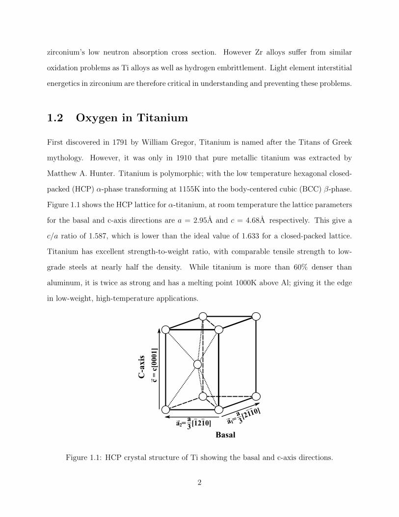
Figure 1.1 shows the HCP lattice for α-titanium, at room temperature the lattice parameters
for the basal and c-axis directions are a = 2.95A and c = 4.68A respectively. This give a
c/a ratio of 1.587, which is lower than the ideal value of 1.633 for a closed-packed lattice.
Titanium has excellent strength-to-weight ratio, with comparable tensile strength to low-
grade steels at nearly half the density. While titanium is more than 60% denser than
aluminum, it is twice as strong and has a melting point 1000K above Al; giving it the edge
in low-weight, high-temperature applications.
c =
c[0
001]
a = [2110]
1
a3a = [1210]2
a3
Basal
C-a
xis
Figure 1.1: HCP crystal structure of Ti showing the basal and c-axis directions.
2

Despite its high strength-to-weight ratio, titanium sees limited use in industry due to its
high cost. This high price is mainly a result of titanium’s high reactivity with oxygen to
form titanium dioxide, requiring complex and expensive processing steps to produce metallic
titanium[6]. However it is also this high oxygen reactivity that leads to the rapid formation
of stable surface oxide layers when titanium is exposed to air, providing excellent corrosion
resistance. As shown in Figure 1.2, the tensile strength of titanium increases with oxygen
content but to the detriment of ductility[4]. These mechanical behavior changes can be
attributed to the interstitial oxygen atoms impeding dislocation motion and inhibiting low-
temperature twinning[7]. As such, oxygen concentration must be carefully controlled in
titanium alloys to obtain desirable properties.
Figure 1.2: Effect of oxygen content on the mechanical properties of titanium[4].
The problem of rapid oxidation stems from both the high chemical affinity of oxygen to
titanium and the high solid solubility of oxygen in α-titanium (up to about 33 at.%)[8], as
3

can be seen in the Ti-O phase diagram (Figure 1.3). As an oxide layer—the scale—forms
on the surface of titanium, the high solubility and affinity creates a continuous oxygen rich
layer—the α-case—adjacent to the scale. At temperatures above 550◦C oxygen transport
through the scales becomes high enough to allow significant growth of the α-case and excess
oxygen to dissolve into titanium.
Introduction
The O-Ti (Oxygen-Titanium) System 15.9994 47.88
By J.L. Murray* National Bureau of Standards and H.A. Wriedt Consultant
This assessment of the Ti-O system covers the phase equi- libria and crystal structures of the condensed phases in the composition range between pure Ti and TiO2. The thermo- dynamic properties of the Ti oxides have been studied and assessed extensively [75Cha]. The present assessment does not duplicate [75Cha]; coverage of thermochemical properties is limited to recent work. So far as possible, melting points and solid-state transition temperatures in the present diagram agree with [75Cha], so that the two assessments may be used together. The assessed Ti-O phase diagram is shown in Fig. 1, and its important features have been summarized in Table 1. The temperature range in which a reasonable equilibrium diagram can be constructed excludes some phase transi- tions of the higher oxides, and it has not been possible to
* Present address: Alcoa Technical Center, Alloy Technology Division, Al- coa Center, PA 15069.
Fig. 1
include all of the observed higher oxide phases in a dia- gram. However, Tables 1, 2, and 3 contain complete list- ings of the phases and phase transitions. O has a large solubility in low-temperature cph (aTi), and it stabilizes (aTi) with respect to the high-temperature bcc form, (flTi). At low temperature, the ordered cph phases Ti20, Ti30, and, possibly, Ti60 are formed with some ho- mogeneity range. Structures of the monoxides are based on the NaC1 struc- ture of the high-temperature yTiO form. Four additional structural modifications were identified, which here are designated flTiO, ~TiO, flTil - xO, and ~Til _ xO. In this as- sessment, "TiO" refers to the monoxides without restric- t ion to a p a r t i c u l a r va r i e ty . The phase bounda r i e s separat ing these phases, except for the disordering of eTiO, were not determined; the phase boundaries of the monoxides in equilibrium with (~Ti) and with flTi203 were de te rmined , but wi thou t d i s t ingu ish ing the var ious monoxide modifications. The stable condensed phase richest in O is rutile (TiO2). In addition to rutile, TiO2 has two nonequilibrium low-pres-
o
<s k, g. E
Assessed Ti-O Phase Diagram
0 2200
W e i g h [ P e r c e n t O x y g e n 10 20 36 40
10 20 30 40 Atomic Percent Oxygen
2000
1800
1600.
1400
1200.
lO00
800-
800-
400 0
Ti 50 60 70
O-Ti
J,L. Murray and H.A. Wriedt, 1987.
148 Bulletin of Alloy Phase Diagrams Vol. 8 No. 2 1987
Figure 1.3: Binary phase diagram for Ti-O[8].
The diffusion of oxygen in titanium impacts the design of implant[9] and aerospace[10]
alloys, as well as the formation of titanium oxides. Increasing the oxygen content in titanium
forms ordered layered-oxide phases, which rely on the diffusion of oxygen into alternating
basal planes to form[11, 12, 13]; modeling the kinetics of ordering[14] requires information
about diffusion. Initial stages of growth of titania nanotubes—e.g., for dye-sensitized solar
cells—via anodization of a titanium metal substrate[15] involves the diffusion of oxygen.
Designing titanium alloys with lower innate oxygen diffusivity has the potential to replace
4

heavier alloys in aerospace to reduce greenhouse-gas emissions. Ultimately, understanding
how to impede or accelerate the diffusion of oxygen requires a fundamental description of
diffusion pathways through titanium.
Diffusion of single oxygen atoms through hexagonal closed-packed (α) titanium initially
appears simple—proposed as atom-hopping between identical interstitial sites, following
an Arrhenius relationship with temperature—but that simplicity hides a complex network
of transition mechanisms. Oxygen prefers to occupy an octahedral interstitial site sur-
rounded by six titanium atoms[7], and so modeling oxygen diffusion had assumed either
direct octahedral-to-octahedral transitions through tetrahedral transition states[16], or from
octahedral to metastable tetrahedral sites[17]. However, the 2005 discovery that the tetra-
hedral site is unstable in favor of a metastable hexahedral site[1] left an open question: how
does interstitial oxygen diffuse through α-titanium? Moreover, the ratio of oxygen diffu-
sivity along basal (xy) directions and the c-axis (z) direction is nearly unity[16] despite no
symmetry relationship between the basal plane and the c-axis.
1.3 Research Scope
This thesis intends to answer the following questions:
• What are all the possible interstitial configurations available to oxygen in the titanium
lattice?
• How does oxygen diffuse between these interstitials?
• How does the oxygen interstitial interact with various solutes in the titanium lattice?
• How do these solute-oxygen interactions affect the diffusion of oxygen through tita-
nium?
• Is it possible to make predictions for the diffusivity of oxygen in arbitrary alloy com-
positions?
5

• How does oxygen behave in HCP elements across the periodic table?
• Are there trends to be found for oxygen energetics in HCP metals?
1.4 Computational Approach
The main computational method for this work is Kohn-Sham density functional theory[18]
(DFT). DFT is an ab initio method in the sense that the energy of the system is only
dependent on atomic positions and identities. This provides a general way for calculating
interactions with arbitrary alloying elements in the periodic table at the atomic scale. In
DFT, the ground state electronic charge density is treated as a basic variable rather than the
full many-body electron wave function, and the energy of the system is a functional of that
charge density. The Hohenberg-Kohn theorem[19] states that the ground state properties
of the many-electron system are uniquely determined by the ground state charge density.
However, it does not describe how to calculate every property from the ground state charge
density or how to compute the charge density for a given system. Kohn-Sham DFT replaces
the many-body electronic wave function with an analogous independent electron system.
The many-body effects of the original system are then grouped together into an effective
exchange-correlation potential. This exchange-correlation potential is typically estimated
from calculations of an electron gas. The LDA exchange-correlation potential uses the
exchange and correlation energies for the electron gas[20] when given the local charge density.
Higher order corrections which also include the local charge density gradient called GGA[21,
22] are also common.
To obtain accurate transition barriers, the nudged elastic band[23] (NEB) method will
be used. NEB is a method to search for the minimum energy pathway between (MEP)
minima on the potential energy surface. Transition barriers determine transition rates and
are inputs to the analytical diffusion equations derived from multi-state diffusion (MSD)
formalism[24, 25]. These equations produce the infinite time diffusion rate for a single
6

particle diffusing through a periodic lattice. This approach is superior to using kinetic
Monte Carlo (KMC), since KMC will only converge to the analytical results in the infinite
time limit, and only for a single temperature. To calculate the effect of solutes on diffusion, a
numerical diffusion model similar to the method described by Allnatt and Lidiard[26] will be
used. This numerical approach will also give the infinite time diffusivity for a given periodic
configuration, though only for a single temperature. Due to the sheer number of possible
solute configurations, their effect on transition barriers will be modeled by the kinetically
resolved activation barrier (KRA) approximation[27] rather than explicitly calculated.
1.5 Outline
In the following chapters a framework is developed for the systematic study of interstitial
energetics and transport in metal lattices. Chapter 2 presents DFT calculation results for
oxygen diffusion in titanium. Where diffusion barriers for all transitions are considered and
combined with analytically derived diffusion equations. Chapter 3 systematically studies
how various solutes across the periodic table interact with oxygen in the titanium lattice.
These interaction energies are applied to a numerical diffusion model from which the effect
on oxygen diffusion due to individual solutes and non-dilute concentrations are predicted.
Chapter 4 extends the study of oxygen interstitial sites and diffusion pathways to all 15 HCP
elements: Be, Cd, Co, Hf, Mg, Os, Re, Ru, Sc, Tc, Ti, Tl, Y, Zn, and Zr (not including
the Lanthanides). Analytical diffusion equations for all systems are derived and surprising
oxygen behavior trends are examined. Chapter 5 summarizes the results for oxygen diffusion
in HCP metals and discusses future directions for additional research.
7

CHAPTER 2
OXYGEN DIFFUSION INTITANIUM
2.1 Computational Method
The ab initio calculations are performed with vasp[28, 29], a plane-wave density-functional
theory (DFT) code. Ti and O are treated with ultrasoft Vanderbilt type pseudopotentials[30,
31] and the generalized gradient approximation of Perdew and Wang[21]. We use a single
oxygen atom in a 96 atom (4×4×3) titanium supercell with a 2×2×2 k-point mesh. A plane-
wave cutoff of 400eV is converged to 0.3meV/atom and the k-point mesh with Methfessel-
Paxton smearing of 0.2eV is converged to 1meV/atom[1]. Projector augmented-wave (PAW)
pseudopotential[32] calculations with the PBE generalized gradient approximation[22] give
similar values, with a maximum error of 0.1eV (see Section 2.3.1). From changes in supercell
stresses for oxygen at different sites, we estimate the finite-size errors to be . 0.05eV; this
is similar to the error found by using different computational cell sizes[1].
The transition rates for individual interstitial jumps are treated with harmonic transition
state theory (HTST). Transition state theory (TST) is a statistical method for calculating
rates of thermally driven processes. TST divides the system phase space into sections with
dividing surfaces bounding each local minima (energetically stable states for the system).
Transitions from one minimum to another occurs when the system crosses over the dividing
surface separating the two states. In HTST the escape rates take the form of an Arrhenius
equation and is written as:
ΛHTST =
∏3Ni νminima
i∏3N−1j νsaddle
j
exp−∆Esaddle
kBT(2.1)
8
where ∆Esaddle is the energy of the saddle point configuration—minimum energy point on
the dividing surface—relative to the current minima configuration. The prefactor is a ra-
tio between the product of all 3N vibrational modes at the current minima and the 3N-1
vibrational modes at the saddle point. One less mode is considered for the saddle point
configuration because the system at that point is unstable along the direction of transition
between the initial state and ending state, and the vibrational mode along that direction is
imaginary. This approximation for the prefactor is known as the Vineyard approximation[33]
and can be thought of as an attempt frequency of the system across the dividing surface in
the direction of transition.
We do not calculate the attempt frequency prefactor for each oxygen transition in the
titanium lattice with all 3N vibrational modes for the system. Only the restoring forces
on the oxygen atom is used to compute the normal mode frequencies. This approximation
leaves out (a) the coupling of oxygen vibration to the Ti vibration, and (b) the softening of
Ti modes due to the relaxation from an interstitial and any electronic effects. To estimate
the errors of ignoring these two terms, we first computed the Vineyard prefactor for oxygen
coupled in a 6× 6× 4 bulk supercell, with the bulk Ti force constants. The Ti-O interaction
is given by the forces on all Ti atoms due to displacement of oxygen from the restoring force
calculation; the Ti atoms affected also have their on-site force constants modified to obey the
sum rule. As oxygen has one-third the mass of Ti, we expect this to be a small correction.
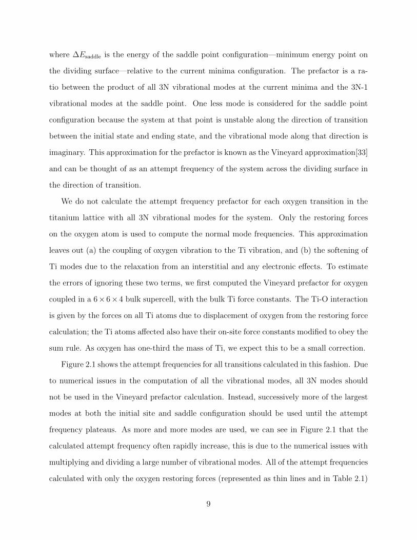
Figure 2.1 shows the attempt frequencies for all transitions calculated in this fashion. Due
to numerical issues in the computation of all the vibrational modes, all 3N modes should
not be used in the Vineyard prefactor calculation. Instead, successively more of the largest
modes at both the initial site and saddle configuration should be used until the attempt
frequency plateaus. As more and more modes are used, we can see in Figure 2.1 that the
calculated attempt frequency often rapidly increase, this is due to the numerical issues with
multiplying and dividing a large number of vibrational modes. All of the attempt frequencies
calculated with only the oxygen restoring forces (represented as thin lines and in Table 2.1)
9

show deviations up to 10–40%, with the largest increase for the o→c transition. Next, we
computed the change in restoring forces for the two Ti atoms closest to the crowdion site,
and at the transition state. When these softer modes are included in the Vineyard prefactor
computation, the o→c prefactor decreased to within 10% of our oxygen-only estimate. This
is the calculation plotted for o→c and c→o in Figure 2.1. Hence, we conservatively estimate
that the absolute prefactors are accurate to within 25%.
0 200 400 600 8000
10
20
30
Atte
mpt
Fre
quen
cy [
TH
z]
O→HH→O
0 200 400 600 8000
10
20
30
Atte
mpt
Fre
quen
cy [
TH
z]
O→CC→O
0 200 400 600 800Number of Largest Modes
0
10
20
30H→CC→H
0 200 400 600 800Number of Largest Modes
0
10
20
30O→O
Figure 2.1: Attempt frequency calculation with Ti force constants. The horizontal axis
represents the number of largest vibrational modes used to compute the Vineyard prefactor
in a 6×6×4 supercell. The thin horizontal lines represent the attempt frequencies calculated
from only the oxygen restoring forces, as tabulated in Table 2.1.
We use the climbing-image nudged elastic band[23, 34] method with one intermediate
image and constant cell shape to find the transition pathways and energy barriers between
different interstitial sites. Nudged elastic band (NEB) is a method to find saddle points
between minima on the potential energy surface. A series of phase space configurations—
images—along the path between the initial and final configurations are optimized to deter-
10

mine the minimum energy pathway (MEP). The images are connected to neighboring images
by spring forces and constrained to relax without perpendicular force components from the
potential. Climbing images nudged elastic band (CI-NEB) is a modification of NEB where
the highest energy image is separated from connecting spring forces and is driven up the
potential energy surface along the direction of the transition, while being minimized in all
other directions. This modification allows an image to converge to the exact saddle point,
the most important configuration to determine for TST. For oxygen transition calculations,
only a single intermediate image was used and forces were relaxed to below 5meV/A. The
use of only a single image for CI-NEB is unusual, and loses entirely the image spring forces
of NEB. This is not desirable for more complicated systems with multi-atom transitions and
unknown transition mechanisms. For the case of oxygen transitions in titanium, we find that
relaxing the saddle point image after a small displacement produce only the initial or final
configurations, depending on the direction of the displacement. This demonstrates that a
single image is sufficient for the simple interstitial transitions that we consider.
2.2 Oxygen Interstitial Sites in Titanium
Figure 2.2 shows the hexagonal closed-packed (HCP) unit cell of α-titanium and the three
interstitial sites for oxygen. The crystal has space group 194, P63/mmc[5]. where the crystal
basis ~a1 and ~a2 are at an angle of 120◦ to each other in the hexagonal (“basal”) plane with
length aTi = 2.933A, while the ~c axis is perpendicular to both with length cTi = 4.638A,
and two titanium atoms per cell. The two titanium atoms occupy the Wyckoff c positions:
(13, 2
3, 1
4) and (2
3, 1
3, 3
4).
11

Site Wyckoff pos.Rnn [A]Z ∆E [eV]
octahedral 2a (0, 0, 0) 2.09 6 +0.00
hexahedral 2d (23 ,
13 ,
14) 1.92 5 +1.19
crowdion 6g (12 , 0, 0) 2.00 6 +1.88
Figure 2.2: Wyckoff positions[5] and relative energies for oxygen interstitial sites in α-
titanium. The interstitial site energy is reported relative to the octahedral site energy. The
geometry of each site is characterized by the nearest neighbor distance after relaxation, Rnn,
with the coordination number Z. Titanium atom sites are in white, while oxygen interstitial
sites are in orange (octahedral), blue (hexahedral), and black (crowdion); the octahedral site
is the ground state, with hexahedral and crowdion having site energies ∆E above. The octa-
hedral sites make a simple hexagonal lattice; the hexahedral sites, a hexagonal closed-packed
lattice; and the crowdion sites, a kagome lattice.
The octahedral (o) site is the equilibrium configuration for oxygen and is surrounded
by 6 titanium atoms in a symmetric arrangement. There are two octahedral site per HCP
unit cell occupying the Wyckoff a positions: (0, 0, 0) and (0, 0, 12). These o-sites form a
hexagonal lattice with a c-axis that is half of the titanium lattice. The octahedral site has
the largest interstitial volume, with a nearest neighbor distance of√
1/2a in the unrelaxed
lattice. With an oxygen occupying the site and after relaxation, the six oxygen-titanium
neighbors are 2.09A away.
The tetrahedral (t) site is the other commonly understood interstitial site in HCP lattices.
There are four equivalent tetrahedral sites per HCP unit cell occupying the Wyckoff f
12

positions: (13, 2
3, 5
8), (1
3, 2
3, 7
8), (2
3, 1
3, 1
8), and (2
3, 1
3, 3
8). The t-sites has nearest neighbor distances
of√
3/8a in the unrelaxed lattice. However, the tetrahedral site is not stable for oxygen in
titanium and atomic forces on the oxygen will displace it towards the basal plane, into the
hexahedral site[1].
The hexahedral (h) site is 5-fold coordinated and is 1.19eV higher in energy than the
o-site. The two equivalent hexahedral sites in each HCP unit cell occupy the Wyckoff d
positions: (13, 2
3, 3
4), and (2
3, 1
3, 1
4). The unrelaxed lattice distances for its three neighbors in
the basal plane is√
1/3a and√
2/3a for the two neighbors in the c-axis. After relaxation,
the three basal titanium neighbors of the h-site displaced to a distance of 1.92A, with two
other neighbors directly above and below at a distance of 2.22A. The h-sites form another
hexagonal closed-packed lattice as α-titanium with a translation of [00012].
The non-basal crowdion (c) site is 6-fold coordinated, but with lower symmetry and
higher energy (1.88eV) than the o-site. There are six equivalent crowdion sites per HCP
unit cell occupying the Wyckoff g positions: (12, 0, 0), (0, 1
2, 0), (1
2, 1
2, 0), (1
2, 0, 1
2), (0, 1
2, 1
2), and
(12, 1
2, 1
2). The crowdion site sits directly in between two nearest neighbor titanium atoms
which are in different basal planes and thus only has an unrelaxed distance of 12a. After
relaxation, the two titanium atoms that contain each c-site are displaced significantly, out
to a distance of 2.00A; the four other titanium neighbors are at a farther distance of 2.18A.
The c-sites form a kagome lattice[35] in the basal plane and is repeated along the c-axis
twice per titanium unit cell. The lowered symmetry of the c-sites in the kagome lattice
mean that a distortion of the unit cell can give the different c-sites different energies. We
also considered a crowdion site in the basal plane, which is unstable. A high formation
energy is required to displace the two titanium atoms into the close-packed directions in the
basal plane, while the two titanium neighbors of the non-basal crowdion can move in the
softer pyramidal plane.
13
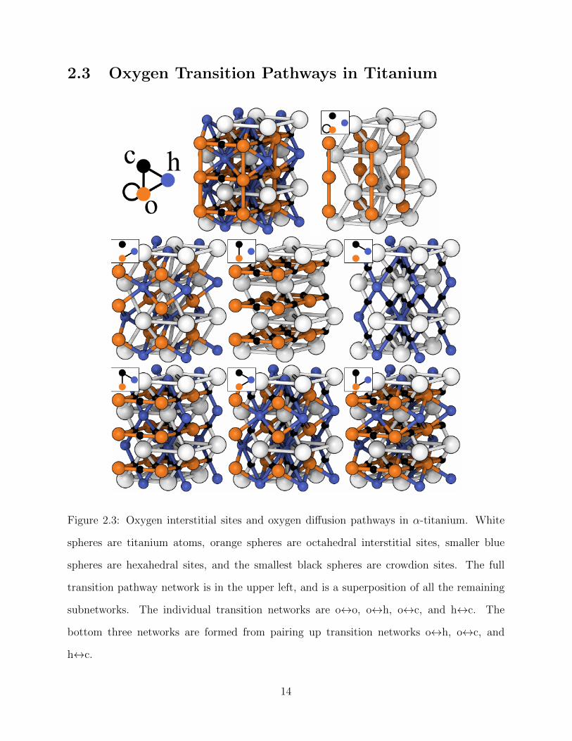
2.3 Oxygen Transition Pathways in Titanium
Figure 2.3: Oxygen interstitial sites and oxygen diffusion pathways in α-titanium. White
spheres are titanium atoms, orange spheres are octahedral interstitial sites, smaller blue
spheres are hexahedral sites, and the smallest black spheres are crowdion sites. The full
transition pathway network is in the upper left, and is a superposition of all the remaining
subnetworks. The individual transition networks are o↔o, o↔h, o↔c, and h↔c. The
bottom three networks are formed from pairing up transition networks o↔h, o↔c, and
h↔c.
14

We considered all possible transition pathways between the three interstitial sites for oxygen
in titanium. Nearest pairs of all possible starting and ending sites were considered. This
process was simplified because the crowdion site is located directly in between all neighboring
pairs of hexahedral sites and basal neighbor pairs of octahedral sites. This means that the
crowdion site act as an intermediate state between those possible transition combinations.
Figure 2.3 show the interpenetrating network of transition pathways for oxygen between
interstitial sites. There are two out-of-plane transitions (with rate λoo) from each o-site with
its two direct neighbors in the c-axis. The o-site is also surrounded by six h-sites and six
c-sites and can transition into them (with rates λoh and λoc). The h-site is surrounded by
six o-sites and six c-sites and can transition into them (with rates λho and λhc). Each c-site
resides in the center of a shared edge between two o-sites and two h-sites and can transition
into them (with rates λco and λch). With the exception of the o↔o c-axis transition, all
other pathways are heterogeneous, starting and ending at different site types, and have not
been considered previously. The transition displacements and surrounding site symmetries
are listing in Table 2.1.
Table 2.1 summarizes the symmetries and energetics of all possible transitions for oxygen
diffusion in α-titanium. The transition rate from site i to j at temperature T is Arrhenius:
λij = νij exp(−Eij/kBT ), where Eij is the energy barrier and νij is the attempt prefactor for
the transition. The barrier of the direct c-axis transition between o-sites—Eoo—is too high
to occur at relevant temperatures. However, the lower barrier o↔h transition also passes
through a triangular face of three titanium atoms like the o↔o c-axis transition. This is sim-
ilar to the instability of basal crowdion sites: the triangular face for the o↔o c-axis transition
requires more energy to displace titanium atoms in the close-packed basal plane. The trian-
gular face for the o↔h transition is in the softer pyramidal plane allowing for easier titanium
atom displacement. Excluding the o↔o c-axis transition, all remaining transitions occur at
approximately the same frequency—there is no single rate-controlling diffusion mechanism.
As the probability of a site i being occupied is proportional to exp(−∆Ei/kBT ) for site
15

Table 2.1: Transition pathways, prefactors ν, and energy barriers E for oxygen diffusionin α-titanium, between octahedral (o), hexahedral (h), and crowdion (c) sites. The direc-tion indicates the possible displacement vectors for the transition; the remaining transitionvectors can be found by applying the point group symmetry operations. The symmetriesare listed in Hermann-Mauguin notation: m is a mirror operation through the basal plane(0001), 1 is inversion, 3 is a 3-fold rotation axis around the c-axis [0001] with inversion, 6is a 6-fold rotation axis around [0001], and 3
mis a 3-fold rotation axis around [0001] with
mirror through (0001). The absolute rate of transitions h→x and c→x is thermally acti-vated with the transition energy barrier plus the site energy for h (+1.19eV) or c (+1.88eV),respectively; hence, all six heterogeneous transitions occur with similar absolute rates.
Direction Symmetry ν [THz] E [eV]o→o 〈0001
2〉 m 11.76 3.25
o→h 〈13
1301
4〉 3 10.33 2.04
o→c 〈16
16
130〉 6 16.84 2.16
h→o 〈13
1301
4〉 3
m5.58 0.85
h→c 〈160 1
614〉 3
m10.27 0.94
c→o 〈16
16
130〉 1 12.21 0.28
c→h 〈160 1
614〉 1 13.81 0.24
energy ∆Ei, the absolute rate of transitions is proportional to exp(−(∆Ei+Eij)/kBT ). The
transition barriers from h- and c-sites are lower than from o-sites, but the occupancy proba-
bility for h- and c-sites are lower. Adding the site energy for h (+1.19eV) and c (+1.88eV) to
the corresponding transition barriers reveal that all transitions occur with a temperature de-
pendence of about ∼2.1eV; hence, all of the interpenetrating transition networks contribute
to the diffusion of oxygen.
2.3.1 Treatment of Oxygen and Titanium in Density-Functional
Theory: USPP and PAW
Table 2.2 shows a comparison of the relative site energies and diffusion barriers for oxy-
gen computed with USPP versus calculations with PAW[32] and the PBE[22] exchange-
correlation potential. The Ti valence is treated as [Mg]3p64s23d2, and the O valence as
[He]2s22p4; these valences are the same for the ultrasoft pseudopotential. As the PAW
16
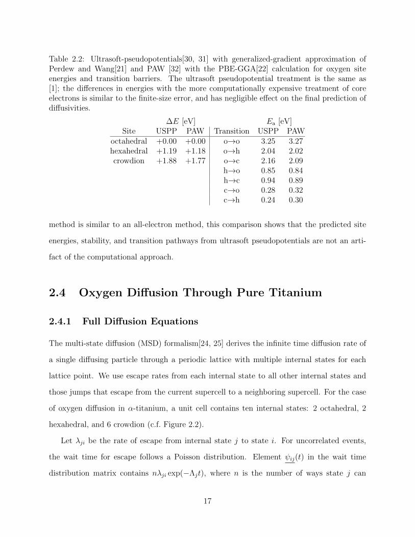
Table 2.2: Ultrasoft-pseudopotentials[30, 31] with generalized-gradient approximation ofPerdew and Wang[21] and PAW [32] with the PBE-GGA[22] calculation for oxygen siteenergies and transition barriers. The ultrasoft pseudopotential treatment is the same as[1]; the differences in energies with the more computationally expensive treatment of coreelectrons is similar to the finite-size error, and has negligible effect on the final prediction ofdiffusivities.
∆E [eV] Ea [eV]Site USPP PAW Transition USPP PAW
octahedral +0.00 +0.00 o→o 3.25 3.27hexahedral +1.19 +1.18 o→h 2.04 2.02crowdion +1.88 +1.77 o→c 2.16 2.09
h→o 0.85 0.84h→c 0.94 0.89c→o 0.28 0.32c→h 0.24 0.30
method is similar to an all-electron method, this comparison shows that the predicted site
energies, stability, and transition pathways from ultrasoft pseudopotentials are not an arti-
fact of the computational approach.
2.4 Oxygen Diffusion Through Pure Titanium
2.4.1 Full Diffusion Equations
The multi-state diffusion (MSD) formalism[24, 25] derives the infinite time diffusion rate of
a single diffusing particle through a periodic lattice with multiple internal states for each
lattice point. We use escape rates from each internal state to all other internal states and
those jumps that escape from the current supercell to a neighboring supercell. For the case
of oxygen diffusion in α-titanium, a unit cell contains ten internal states: 2 octahedral, 2
hexahedral, and 6 crowdion (c.f. Figure 2.2).
Let λji be the rate of escape from internal state j to state i. For uncorrelated events,
the wait time for escape follows a Poisson distribution. Element ψij(t) in the wait time
distribution matrix contains nλji exp(−Λjt), where n is the number of ways state j can
17

reach the same equivalent state i in different supercells, and Λj is the sum of all transition
rates from state j. The Laplace transform of the waiting time density matrix, ψ(u), is
ψ(u) =
o1 o2 h1 h2 c1 c2 c3 c4 c5 c6
o1
0 2λoo
u+Λo
3λho
u+Λh
3λho
u+Λh
2λco
u+Λc
2λco
u+Λc
2λco
u+Λc0 0 0
o22λoo
u+Λo0 3λho
u+Λh
3λho
u+Λh0 0 0 2λco
u+Λc
2λco
u+Λc
2λco
u+Λc
h13λoh
u+Λo
3λoh
u+Λo0 0 λch
u+Λc
λch
u+Λc
λch
u+Λc
λch
u+Λc
λch
u+Λc
λch
u+Λc
h23λoh
u+Λo
3λoh
u+Λo0 0 λch
u+Λc
λch
u+Λc
λch
u+Λc
λch
u+Λc
λch
u+Λc
λch
u+Λc
c12λoc
u+Λo0 λhc
u+Λh
λhc
u+Λh0 0 0 0 0 0
c22λoc
u+Λo0 λhc
u+Λh
λhc
u+Λh0 0 0 0 0 0
c32λoc
u+Λo0 λhc
u+Λh
λhc
u+Λh0 0 0 0 0 0
c4 0 2λoc
u+Λo
λhc
u+Λh
λhc
u+Λh0 0 0 0 0 0
c5 0 2λoc
u+Λo
λhc
u+Λh
λhc
u+Λh0 0 0 0 0 0
c6 0 2λoc
u+Λo
λhc
u+Λh
λhc
u+Λh0 0 0 0 0 0
(2.2)
where
Λo = 2λoo + 6λoh + 6λoc
Λh = 6λho + 6λhc
Λc = 2λco + 2λch
For each jump we specify whether the diffusing particle has left the supercell. For a 3D
periodic supercell, let ~be the supercell position of the particle and ~j−~i = m1~l1+m2
~l2+m3~l3
be the supercell displacement vector after jumping from site i to j. The ~lr are the orthogonal
supercell vectors with length lr in the r direction (r = 1, 2, 3). The transitions in each element
of the matrix ψ(u) have the same degenerate rate, but can go to different supercells. Each ele-
18

ment pij(~) contains the average displacement from the corresponding element ψij
(u). For the
ij element, we use the shorthand δm1m2m3 ≡ δ`j1−`i1,m1δ`j2−`i2,m2
δ`j3−`i3,m3. The Fourier transform
of p(~) is p∗(~k); and δm1m2m3 is transformed into exp (i (m1l1 · k1 +m2l2 · k2 +m3l3 · k3)).
Then,
p(~) =
o1 o2 h1 h2 c1 c2 c3 c4 c5 c6
o1
0 δ000+δ001
2δ000+δ010+δ100
3δ000+δ100+δ110
3δ000+δ100
2δ000+δ010
2δ010+δ100
20 0 0
o2δ000+δ001
20 δ001+δ011+δ101
3δ000+δ100+δ110
30 0 0 δ000+δ100
2δ000+δ010
2δ010+δ100
2
h1δ000+δ100+δ010
3δ001+δ101+δ011
30 0 δ000 δ000 δ000 δ001 δ001 δ001
h2δ000+δ100+δ110
3δ000+δ100+δ110
30 0 δ000 δ110 δ010 δ000 δ110 δ010
c1δ000+δ100
20 δ000 δ000 0 0 0 0 0 0
c2δ000+δ010
20 δ000 δ110 0 0 0 0 0 0
c3δ010+δ100
20 δ000 δ010 0 0 0 0 0 0
c4 0 δ000+δ100
2δ001 δ000 0 0 0 0 0 0
c5 0 δ000+δ010
2δ001 δ110 0 0 0 0 0 0
c6 0 δ010+δ100
2δ001 δ010 0 0 0 0 0 0
(2.3)
We construct the matrix R(~k, u) and its determinant ∆(~k, u),
Rij(~k, u) =
[I ij − ψij(u) · p∗
ij(~k)]
(2.4)
∆(~k, u) = det[R(~k, u)
](2.5)
where I is the identity matrix. With the Laplace and Fourier transform, we get to the limit
of t→∞ as u→ 0 and the limit of ~→∞ as ~k → 0. We first find the leading term in the
long-time limit, ∆0(~k),
∆0(~k) = limu→0
∆(~k, u)
u. (2.6)
19

Then the variance of diffusion in the r direction is:
σ2r(t) ≡ 〈`2(t)〉r − 〈`(t)〉2r = lim
~k→0t
1
∆0
δ2∆
δk2r
∣∣∣∣∣u→0
(2.7)
We can get the diffusion equations directly from the diffusion variance by dividing out a
factor of 2t,
Dr =σ2r(t)
2t(2.8)
We now take the orthogonal supercell coordinates back to the hexagonal unit cell by a metric
tensor transform,
Dx = D1 −1
4D2 (2.9)
Dy =3
4D2 (2.10)
Dz = D3 (2.11)
Diffusion in the basal plane is isotropic, so D1 = D2, and the full diffusion equations are
Dbasal = Dx = Dy =
a2Ti
1
4
4λhoλohλch + λhcλohλch + 4λhcλohλco + 4λhoλohλco + 4λhoλocλch + λhcλocλch + 3λhoλocλco + 3λhcλocλco
λohλco + 3λhcλoh + λohλch + λhoλco + λcoλhc + λocλch + λhoλch + 3λhcλoc + 3λhoλoc
(2.12)
Dc = Dz =
c2Ti
1
8
3λhoλohλco + 3λhcλohλco + 3λhcλohλch + 3λhoλohλch + 2λhoλooλco + 2λhcλooλco + 2λhoλooλch + 3λhcλocλch + 3λhoλocλch
λohλco + 3λhcλoh + λohλch + λhoλco + λcoλhc + λocλch + λhoλch + 3λhcλoc + 3λhoλoc
(2.13)
As the octahedral site is the lowest in energy, when kBT is small compared to the difference
in activation energies from o→h and h→o, then λhc and λch are much greater than λoh and
λoc, and the diffusion reduces to the simplified Eqn. (2.14) and Eqn. (2.15):
20
Dbasal = a2Ti
[λoh +
3
4λoc +
1
4
λoh
λho
λhc + 0λoo
](2.14)
Dc = c2Ti
[3
8λoh + 0λoc +
3
8
λoh
λho
λhc +1
4λoo
](2.15)
After simplification, it becomes clear that the diffusion equations correspond to the sum
of the individual diffusion networks of Figure 2.3. Going from left to right in Eqn. (2.14)
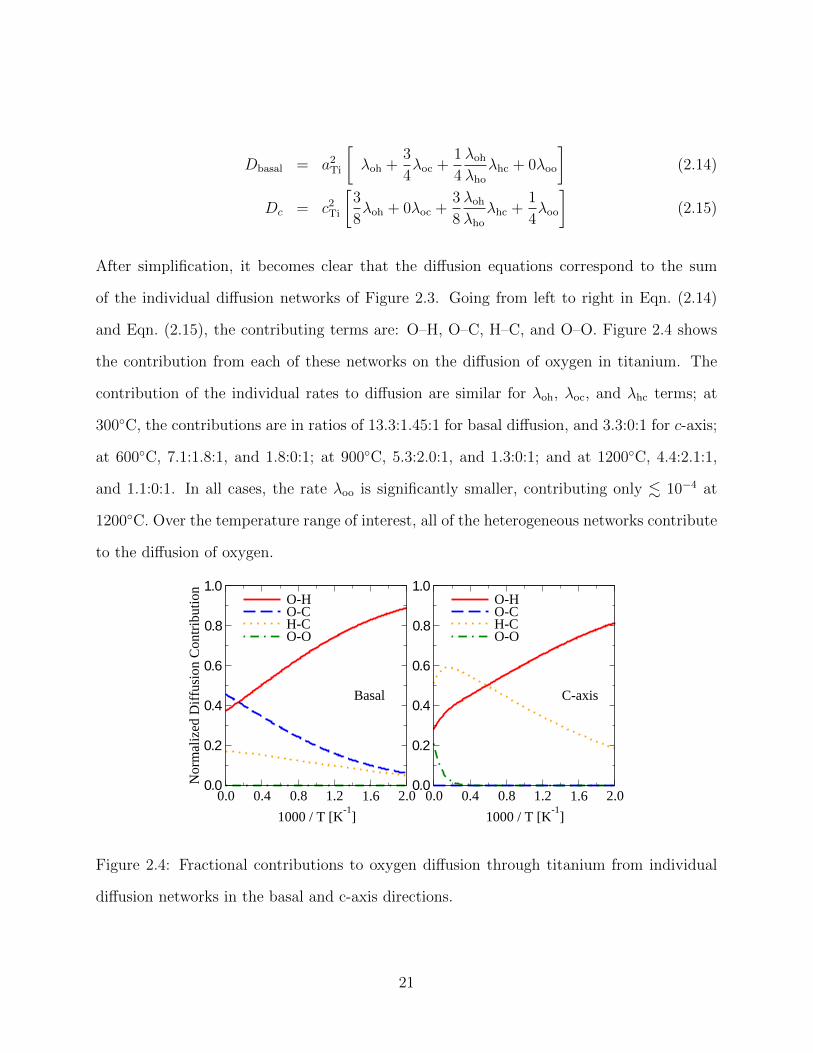
and Eqn. (2.15), the contributing terms are: O–H, O–C, H–C, and O–O. Figure 2.4 shows
the contribution from each of these networks on the diffusion of oxygen in titanium. The
contribution of the individual rates to diffusion are similar for λoh, λoc, and λhc terms; at
300◦C, the contributions are in ratios of 13.3:1.45:1 for basal diffusion, and 3.3:0:1 for c-axis;
at 600◦C, 7.1:1.8:1, and 1.8:0:1; at 900◦C, 5.3:2.0:1, and 1.3:0:1; and at 1200◦C, 4.4:2.1:1,
and 1.1:0:1. In all cases, the rate λoo is significantly smaller, contributing only . 10−4 at
1200◦C. Over the temperature range of interest, all of the heterogeneous networks contribute
to the diffusion of oxygen.
0.0 0.4 0.8 1.2 1.6 2.0
1000 / T [K-1
]
0.0
0.2
0.4
0.6
0.8
1.0
Nor
mal
ized
Dif
fusi
on C
ontr
ibut
ion
O-HO-CH-CO-O
0.0 0.4 0.8 1.2 1.6 2.0
1000 / T [K-1
]
0.0
0.2
0.4
0.6
0.8
1.0O-HO-CH-CO-O
Basal C-axis
Figure 2.4: Fractional contributions to oxygen diffusion through titanium from individual
diffusion networks in the basal and c-axis directions.
21

0.0 0.5 1.0 1.5 2.01000 / T [K
-1]
0.7
0.8
0.9
1.0
1.1
1.2
1.3
Dc-
axis /
Dba
sal
1200oC1200
oC 500
oC 300
oC
experimental dataanalytical model
Figure 2.5: C-axis vs. basal diffusion ratios from our diffusion model and experimentally
measured diffusion anisotropy values[13].
Figure 2.5 shows that our diffusion equations predict nearly isotropic diffusion between
the c-axis and basal directions. This is slightly surprising as there is no crystallographic
relationship for diffusion between these directions in the HCP lattice. The obtained near
isotropy is due to the fact that the O–H and H–C diffusion networks contribute significantly
to both c-axis and basal diffusion. Also, while both O–C and O–O diffusion networks are
anisotropic, their contributions are less than the other networks. However experimental
data on the diffusion anisotropy[13] shows that while the measured ratio is close to unity,
there is much more variation with temperature than our predictions. It is not known where
the source of the discrepancy lies, as many different combination of transition barrier and
attempt frequency errors can lead to the observed effect. More accurate calculations and
further experimental measurements are needed.
22

0.4 0.8 1.2 1.6 2.01000 / T [K
-1]
0.8
1.0
1.2
1.4
1.6
Dby
-pas
s / D
full
1200°C 800°C 500°C 300°C
by-pass model
Figure 2.6: Oxygen diffusion in titanium when assuming the crowdion site is by-passed
(Eqn. (2.16) and Eqn. (2.17)), normalized to the full diffusion equations (Eqn. (2.14) and
Eqn. (2.15)).
The full diffusion equations have been derived with the assumption that the crowdion
sites are able to thermalize, and thus there are no correlated hops from the crowdion sites to
neighboring sites. As temperature increases, we do not expect the crowdion site to achieve
thermal equilibrium; hence, an increasing fraction of o→c jumps will become correlated basal
o→o jumps, and h→c jumps will become correlated h→h jumps. This high temperature
behavior can be approximated by removing the crowdions as metastable states from the
network, and using λoc as the rate for direct basal o→o transitions (and similarly λhc for
h→h transitions). Then, the diffusion rates are bounded above by
Dhigh Tbasal / a2
Ti
[λoh +
3
2λoc +
1
2
λoh
λho
λhc + 0λoo
](2.16)
Dhigh Tc / c2
Ti
[3
8λoh + 0λoc +
3
4
λoh
λho
λhc +1
4λoo
](2.17)
Diffusion calculated from these by-pass equations is plotted in Figure 2.6. At 1200◦C, the
high temperature Eqn. (2.16) is 41% larger than Eqn. (2.14) and Eqn. (2.17) is 48% larger
23

than Eqn. (2.15); at 300◦C, the differences are only 16% and 23%. This suggests a small
underestimation of diffusion rates at the highest temperatures.
2.4.2 Diffusivity Through Subnetworks
Diffusion through each of the three individual networks and their complement networks have
been computed using the same multistate diffusion method above. Approximations can be
made to the full diffusion equations to produce the simplified Eqn. (2.14) and Eqn. (2.15).
Applying the same simplifications to the subnetworks gives:
Dbasal ≈ a2Ti λoh
Dc ≈ c2Ti
3
8λoh
Dbasal ≈ a2Ti
3
4λoc
Dc = 0
Dbasal ≈ a2Ti
1
4
λoh
λhoλhc
Dc ≈ c2Ti
3
8
λoh
λhoλhc
Dbasal ≈ a2Ti
(3
4λoc +
1
4
λoh
λhoλhc
)Dc ≈ c2Ti
3
8
λoh
λhoλhc
Dbasal ≈ a2Ti
(λoh +
1
4
λoh
λhoλhc
)Dc ≈ c2Ti
3
8
(λoh +
λoh
λhoλhc
) Dbasal ≈ a2Ti
(λoh +
3
4λoc
)Dc ≈ c2Ti
3
8λoh
Figure 2.7: Approximate analytical diffusion equations for sub-networks from Figure 2.3.
The h↔c only network does not contain octahedral sites and we must multiply the occupancy
24

probability of the h-site (λoh/λho) to arrive at the absolute rate of transition. Note also that
λohλhcλco = λocλchλho by detailed balance. Adding the transition networks results in the
simplified equations Eqn. (2.14) and Eqn. (2.15).
0.6 0.8 1 1.2 1.4 1.6 1.8
1000 / T [K-1
]
!"!##
!"!#"
!"!!$
!"!!%
!"!!&
!"!!#
!"!!"
Dif
fusi
on c
oef
fici
ent
[m2/s
]
1200'C 900'C 600'C 300'C
Bregolin et. al. (2007)
Vykhodets et. al. (1989)
Liu and Welsch (1957-1983)
Analytical Model
Figure 2.8: Analytical results and experimental data of oxygen diffusivity in α-titanium. We
compare our analytical DFT model (bold line) to experimental data from the literature sur-
vey by Liu and Welsch[36] (thin lines), and experiments by Bregolin[37] and Vykhodets[38]
(symbols). Over the temperature range of 300–1200◦C, the diffusion rate is Arrhenius D0 =
2.18×10⁻⁶ m2s−1 with Eact = 2.08eV.
Figure 2.8 shows the diffusion coefficient from the multistate diffusion equations against
experimental oxygen diffusion data. From the diffusion equations Eqn. (2.14) and Eqn. (2.15),
the temperature behavior should follow the barriers, Eoh, Eoc, and Ehc + Eoh − Eho. An
Arrhenius model with D0 = 2.18 × 10⁻⁶m2/s and a single barrier Eact = 2.08eV matches
Eqn. (2.14) and Eqn. (2.15) to within 15% over the range 300–1200◦C, with largest deviations
at low temperatures. The experimental data come from the literature survey[36] by Liu and
25

Welsch and more recent experiments[37, 38] using nuclear reaction analysis. The activation
energy matches well to experiment while the absolute diffusion coefficient is a factor of ten
below experimental values—well within the expected accuracy of density-functional theory
for diffusion.
2.5 Summary
Ab initio calculations determine the pathways for oxygen diffusion in α-titanium, including a
new interstitial non-basal crowdion site for oxygen in titanium. Other than the high-barrier
direct c-axis transition between octahedral sites, all transition paths are heterogeneous (o↔h,
o↔c, and h↔c) and contribute to diffusion over a wide temperature range. This shows that
even well-studied materials science problems can have surprises: new configurations and new
transitions give rise to complexity for single atom diffusion. Moreover, the new sites suggests
that interesting interactions with titanium vacancies are possible, as they should destabilize
nearby crowdion and perhaps hexahedral sites. We expect other interstitial elements like
carbon and nitrogen to have similar diffusion networks in titanium, and in other hexagonal-
closed packed metals like magnesium and zirconium. This new understanding of oxygen in
titanium can serve as the basis for controlling oxygen diffusion in alloys, growth of oxide
phases in titanium, and related challenges.
26

CHAPTER 3
EFFECT OF SOLUTES ONOXYGEN DIFFUSION THROUGH
TITANIUM
3.1 Computational Method
3.1.1 Pseudopotential Valence For Computed Solutes
Table 3.1 summarizes all solutes that were considered in this work and their pseudopotential
valence configurations. The Ti valence is treated as 3p63d24s2, and the O valence as 2s22p4.
All solutes used ultrasoft pseudopotentials, with the exception of Ge, La, Mn, and Na.
Table 3.1: Substitutional solutes and their pseudopotential valence configurations. Solutesfollowed by an * are treated with PAW, all others are treated with USPP.
Valence ConfigurationsAg 4d105s1 Al 3s23p1 Au 5d106s1 Ba 5s25p66s2 Ca 3p64s2
Cd 4d105s2 Co 3d74s2 Cr 3d54s1 Cs 5p66s1 Cu 3d104s1
Fe 3d64s2 Ga 3d104s24p1 Ge* 4s24p2 Hf 5d26s2 Hg 5d106s2
In 4d105s25p1 Ir 5d86s1 K 3p64s1 La* 5s25p65d16s2 Mg 2p63s2
Mn* 3p63d64s1 Mo 4p64d55s1 Na* 2p63s1 Nb 4p64d45s1 Ni 3d84s2
Os 5d66s2 Pb 5d106s26p2 Pd 4d95s1 Pt 5d96s1 Rb 4p65s1
Re 5d56s2 Rh 4d85s1 Ru 4d75s1 Sc 3p63d24s1 Si 3s23p2
Sn 4d105s25p2 Sr 4p65s2 Ta 5d36s2 Tc 4d55s2 Tl 5d106s26p1
V 3p63d34s2 W 5d46s2 Y 4p64d15s2 Zn 3d104s2 Zr 4p64d35s1
27
3.1.2 Kinetically Resolved Activation Barrier Approximation
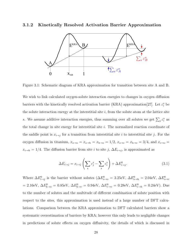
Figure 3.1: Schematic diagram of KRA approximation for transition between site A and B.
We wish to link calculated oxygen-solute interaction energies to changes in oxygen diffusion
barriers with the kinetically resolved activation barrier (KRA) approximation[27]. Let εsi be
the solute interaction energy at the interstitial site i, from the solute atom at the lattice site
s. We assume additive interaction energies, thus summing over all solutes we get∑
s εsi as
the total change in site energy for interstitial site i. The normalized reaction coordinate of
the saddle point is xi→j for a transition from interstitial site i to interstitial site j. For the
oxygen diffusion in titanium, xo→o = xo→h = xh→o = 1/2, xo→c = xh→c = 3/4, and xc→o =
xc→h = 1/4. The diffusion barrier from site i to site j, ∆Ei→j, is approximated as
∆Ei→j = xi→j
(∑s
εsj −∑s
εsi
)+ ∆E0
i→j. (3.1)
Where ∆E0i→j is the barrier without solutes (∆E0
o→o = 3.25eV, ∆E0o→h = 2.04eV, ∆E0
o→c
= 2.16eV, ∆E0h→o = 0.85eV, ∆E0
h→c = 0.94eV, ∆E0c→o = 0.28eV, ∆E0
c→h = 0.24eV). Due
to the number of solutes and the multitude of different combination of solute position with
respect to the sites, this approximation is used instead of a large number of DFT calcu-
lations. Comparison between the KRA approximation to DFT calculated barriers show a
systematic overestimation of barriers by KRA; however this only leads to negligible changes
in predictions of solute effects on oxygen diffusivity, the details of which is discussed in
28

Section 3.6.
Changes in diffusivity are calculated numerically using a similar method as described
by Allnatt and Lidiard[26]. The main idea behind this method comes from the Einstein-
Smoluchowski diffusion relation[39, 40]. A diffusing species under the influence of a uniform
bias field will move in direct proportion to the strength of the applied field under linear
response theory. At equilibrium the drift flux due to the applied field will be equal to the
random diffusion flux. Therefore, if the drift flux due to the applied external field can be
computed, then the diffusivity is obtained as well. Because the bias field changes the site
transition rates and in turn the site occupancy probabilities, the drift flux calculation is not
straightforward and must be done numerically.
We choose a temperature of 900K for an isolated solute in 9× 9× 9, 10× 10× 10, and
11×11×11 supercells. These correspond to solute concentrations of 6.86×10⁻⁴, 5.00×10⁻⁴,
and 3.76× 10⁻⁴ respectively. We define the infinite dilute solute effect as
∆D =1
D0
dD(c)
dc
∣∣∣∣c=0
, (3.2)
where D(c) is the diffusivity at solute concentration c, and D0 is the solute free diffusivity.
A quadratic fit of the diffusivity is done at the three concentrations above with the linear
term being ∆D.
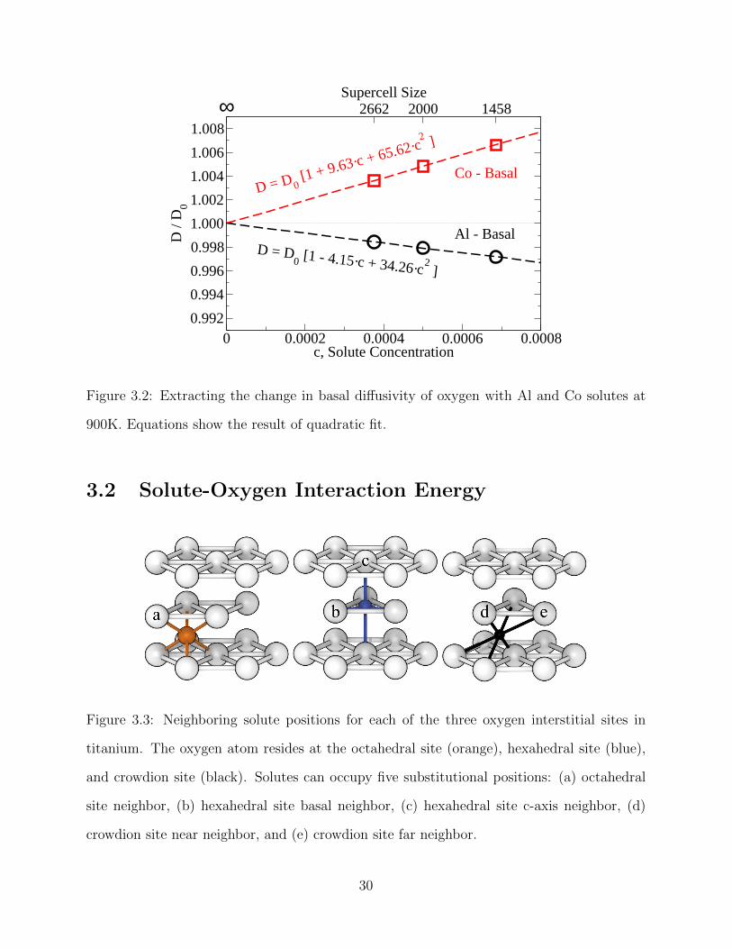
Figure 3.2 shows an example of the fitting procedure for the basal diffusion of oxygen
with Al and Co solutes. The fitting is constrained to satisfy D(c)/D0 = 1 at c=0.
29
0 0.0002 0.0004 0.0006 0.0008c, Solute Concentration
0.992
0.994
0.996
0.998
1.000
1.002
1.004
1.006
1.008
D /
D0
∞ 2662 2000 1458Supercell Size
Co - Basal
Al - BasalD = D
0 [1 - 4.15·c + 34.26·c2 ]
D = D0 [1 + 9.63·c + 65.62·c2 ]
Figure 3.2: Extracting the change in basal diffusivity of oxygen with Al and Co solutes at
900K. Equations show the result of quadratic fit.
3.2 Solute-Oxygen Interaction Energy
Figure 3.3: Neighboring solute positions for each of the three oxygen interstitial sites in
titanium. The oxygen atom resides at the octahedral site (orange), hexahedral site (blue),
and crowdion site (black). Solutes can occupy five substitutional positions: (a) octahedral
site neighbor, (b) hexahedral site basal neighbor, (c) hexahedral site c-axis neighbor, (d)
crowdion site near neighbor, and (e) crowdion site far neighbor.
30
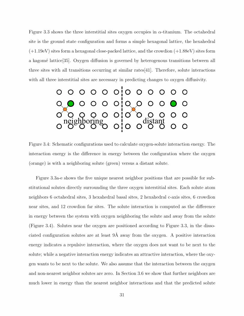
Figure 3.3 shows the three interstitial sites oxygen occupies in α-titanium. The octahedral
site is the ground state configuration and forms a simple hexagonal lattice, the hexahedral
(+1.19eV) sites form a hexagonal close-packed lattice, and the crowdion (+1.88eV) sites form
a kagome lattice[35]. Oxygen diffusion is governed by heterogenous transitions between all
three sites with all transitions occurring at similar rates[41]. Therefore, solute interactions
with all three interstitial sites are necessary in predicting changes to oxygen diffusivity.
neighboring distant
Figure 3.4: Schematic configurations used to calculate oxygen-solute interaction energy. The
interaction energy is the difference in energy between the configuration where the oxygen
(orange) is with a neighboring solute (green) versus a distant solute.
Figure 3.3a-e shows the five unique nearest neighbor positions that are possible for sub-
stitutional solutes directly surrounding the three oxygen interstitial sites. Each solute atom
neighbors 6 octahedral sites, 3 hexahedral basal sites, 2 hexahedral c-axis sites, 6 crowdion
near sites, and 12 crowdion far sites. The solute interaction is computed as the difference
in energy between the system with oxygen neighboring the solute and away from the solute
(Figure 3.4). Solutes near the oxygen are positioned according to Figure 3.3, in the disso-
ciated configuration solutes are at least 9A away from the oxygen. A positive interaction
energy indicates a repulsive interaction, where the oxygen does not want to be next to the
solute; while a negative interaction energy indicates an attractive interaction, where the oxy-
gen wants to be next to the solute. We also assume that the interaction between the oxygen
and non-nearest neighbor solutes are zero. In Section 3.6 we show that further neighbors are
much lower in energy than the nearest neighbor interactions and that the predicted solute
31

Table 3.2: Table of oxygen-solute interaction energies for different oxygen and solute con-figurations. Interaction energies are reported in units of eV, a positive value correspondsto a repulsive interaction between the oxygen and the solute, negative value indicates anattractive interaction, while ’-----’ indicates that the particular oxygen-solute configurationdestabilizes the interstitial site. Interactions are ordered as follows: octahedral site neighbor,hexahedral site basal neighbor, hexahedral site c-axis neighbor, crowdion site near neighbor,and crowdion site far neighbor.
Na+0.04+0.12-0.45+0.26-0.29
K+0.09+0.02-0.51+0.61-0.51
Rb+0.18+0.31-0.45+0.69-0.48
Cs+0.61+0.42-0.28+1.61-----
Mg+0.25+0.21-0.13+0.29+0.02
Ca-0.01+0.09-0.41+0.51-0.44
Sr+0.08+0.02-0.44+0.67-0.54
Ba+0.38+0.33-0.31+0.95-0.38
Sc-0.03+0.06-0.22+0.32-0.22
Y+0.10+0.21-0.28+0.66-0.36
La+0.23+0.14-0.27+0.51-0.44
Ti+0.00+0.00+0.00+0.00+0.00
Zr+0.13+0.31-0.08+0.41-0.14
Hf+0.07+0.20-0.06+0.35-0.10
V+0.09-0.06+0.16-0.33+0.15
Nb+0.23+0.30+0.10+0.14+0.08
Ta+0.22+0.29+0.16+0.15+0.13
Cr+0.20-0.23+0.24-0.71+0.20
Mo+0.35+0.16+0.04-0.13+0.24
W+0.44+0.25+0.22-0.04+0.33
Mn+0.44-0.22+0.04-0.76+0.38
Tc+0.65+0.16+0.08-0.15-----
Re+0.72+0.27+0.21-0.02-----
Fe+0.34-0.27-0.00-0.73-----
Ru+0.48-0.06-0.05+0.01-----
Os+0.70+0.18+0.19+0.09-----
Co+0.34-0.36-0.10-0.28-----
Rh+0.53+0.02-0.00+0.34-----
Ir+0.62+0.06+0.08+0.50-----
Ni+0.50+0.01+0.04+0.05-----
Pd+0.65+0.44+0.02+0.74-----
Pt+0.76+0.41+0.14+0.89-----
Cu+0.57+0.40+0.05+0.36-----
Ag+0.68+0.81-0.03+0.98-----
Au+0.82+0.83+0.08+1.15-----
Zn+0.64+0.61+0.10+0.60-----
Cd+0.74+1.00+0.02+1.15-----
Hg+0.85+1.10+0.08+1.32-----
Ga+0.83+0.81+0.27+0.90-----
Al+0.72+0.46+0.26+0.51-----
In+0.88+1.18+0.17+1.40-----
Tl+0.92+1.25+0.15+1.48-----
Si+0.97+0.87+0.46+1.03-----
Ge+0.94+0.99+0.41+1.27-----
Sn+1.02+1.36+0.32+1.67-----
Pb+1.00+1.40+0.25+1.71-----
3
4
5
6
1 2
3 4 5 6 7 8 9 10 11 12
13 14Soluteoctahedralhexahedral basalhexahedral c-axiscrowdion nearcrowdion far
effects on oxygen diffusivity do not change significantly after including additional neighbor
interactions.
Table 3.2 and Figure 3.5 shows the solute interaction energies for elements across the
periodic table. The octahedral site (Figure 3.5a) with a distance of 2.09A between oxygen
and solute, gives an interaction energy that is repulsive for almost all solutes. Only Ca and
Sc are weakly attractive for oxygen in the titanium lattice. Given the high affinity oxygen has
for titanium, it is not surprising that almost no other element has an attractive interaction
as a substitutional solute. Because the octahedral site is the ground-state interstitial site for
oxygen, this means that almost no solutes act as traps for oxygen in titanium. The trend
observed shows an increase in repulsion with more d-electron filling and with higher period.
32

Figure 3.5: Plot of oxygen-solute interaction energies for different oxygen interstitials and so-
lute configurations. Periodic table groups are plotted along the horizontal axis while periodic
table periods are separated into different symbols. Positive energies correspond to repulsive
interactions between the oxygen and the solute, while negative energies indicates an attrac-
tive interaction. Solute positions correspond to Figure 3.3: (a) octahedral site neighbor, (b)
hexahedral site basal neighbor, (c) hexahedral site c-axis neighbor, (d) crowdion site near
neighbor, and (e) crowdion site far neighbor.
33
The interaction energy between oxygen and solutes at the hexahedral basal site (Fig-
ure 3.5b), with a oxygen-solute distance of 1.92A, forms a V-shaped curve with the dip at
near half d-filling. A gradually increasing attractive interaction is seen for solutes up to half
d-filling, after which the interactions become significantly repulsive with higher d-filling. The
4th period exhibits a more attractive interaction than either the 5th or 6th period.
Transition metal solutes at the hexahedral c-axis site (Figure 3.5c), with a oxygen-solute
distance of 2.22A, do not interact strongly with oxygen. A slight attractive interaction is
seen for the larger alkali and alkaline earth metals, while a slight repulsion is seen for the
smaller post-transition metals. The hexahedral c-axis site is further away from the oxygen
than the basal neighbor which explains its low interaction with most solute, its attraction
to larger solute, and its repulsion of smaller atoms.
The crowdion near site (Figure 3.5d), with a oxygen-solute distance of 2.00A, behaves
similarly to the hexahedral basal site, with a V-shaped interaction curve dipping at near half
d-filling. This similar behavior stems from the close proximity both the hexahedral basal
site and the crowdion near site have with the oxygen atom. Both V-shaped curves correlates
to the dip in atomic radii for the middle transition metals. Compared to the hexahedral
basal site, solutes at the crowdion near site exhibit a more dramatic dip at half d-filling as
well as a larger disparity between the 4th period and the other periods.
Most solutes at the crowdion far site (Figure 3.5e), with a oxygen-solute distance of
2.18A, destabilize the crowdion site for oxygen. Unlike the crowdion near site, where the
oxygen atom is confined directly between the solute and a titanium atom, a solute at the
far site pushes the oxygen closer to neighboring octahedral and hexahedral sites. Since the
barrier to leave the crowdion site is only 0.24–0.28eV, inspecting Table 3.2 shows that almost
no stable far site solute has a higher interaction energy. This is because the far site solute
positions displaces the already low symmetry crowdion interstitial. Since the crowdion far
site is also further away from the oxygen than the near neighbor, we would expect it to behave
similar to the hexahedral c-axis site. For solutes which do not destabilize the interstitial this
34
is shown to be the case, as an attractive interaction is seen for the larger alkali and alkaline
earth metals.
Most solute atoms substitute directly to the Ti HCP lattice position, however there are
four elements which do not. The mid-transition HCP metals: Os, Re, Ru, and Tc take up
a lower energy, asymmetric configuration when they substitute for a Ti atom. While these
elements are still metastable at the position of the replaced lattice atom, their ground-state
configuration is∼0.5A away in the [0001] (Ru) or [1230] (Os, Re, and Tc) directions. We have
not investigated whether these off-center sites are a general result across pseudopotentials
or valences. All interaction energies for these four elements are calculated with these solutes
at the off-center configurations.
3.3 Numerical Diffusion Model Predictions
-0.8 -0.4 0.0 0.4 0.8
-10
0
10
20
30
∆D
[%/%]
BasalC-axis
-0.8 -0.4 0.0 0.4 0.8 -0.8 -0.4 0.0 0.4 0.8Solute Interaction Energy [eV]
-0.8 -0.4 0.0 0.4 0.8 -0.8 -0.4 0.0 0.4 0.8
-980
-65
-4650
-6000
Figure 3.6: Predicted diffusivity changes for oxygen in titanium at 900K for individual solute
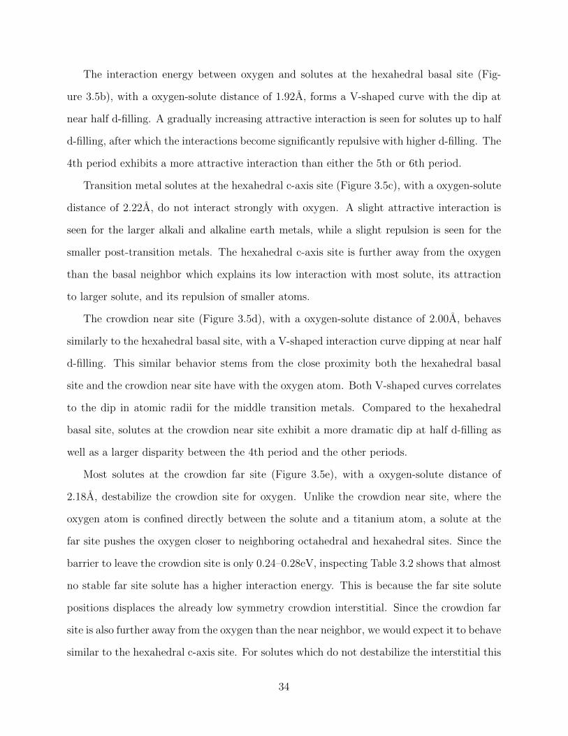
neighbor interactions. The basal and c-axis diffusion changes are reported as percent change
in oxygen diffusivity per atomic percent solute concentration, at the infinite dilute limit.
The leftmost plot is for the octahedral neighbor and both diffusivities are highly reduced for
negative solute interactions, (–0.2eV, –65), (–0.4eV, –980), (–0.6eV, –4650), and (–0.8eV,
–6000).
35

Figure 3.6 shows the effect of the individual solute neighbor interactions on oxygen dif-
fusion in titanium for both basal and c-axis diffusion. These values are calculated from
our numerical model with only a single solute neighbor interaction set as non-zero. The
ground-state octahedral site shows the largest effect on oxygen diffusion. At negative solute
interactions—trapping for the octahedral site—oxygen diffusivity for both basal and c-axis
are significantly reduced. At positive octahedral interactions, the c-axis diffusion is accel-
erated while the basal diffusion initially accelerates, but becomes reducing at higher solute
interactions. The accelerating effects come from an increase in the rates out of the affected
octahedral sites to hexahedral sites which is not completely offset by the decrease in the
rates into the octahedral from crowdion sites.
Negative interactions for the metastable site neighbors, hexahedral and crowdion, shows
an accelerating effect on oxygen diffusion in titanium. A detailed explanation for this ac-
celerating effect is given in Section 3.4. Changes in diffusivity for both basal and c-axis
directions are similar for almost all interactions. The exception is the hexahedral basal site,
which has a larger accelerating effect for basal diffusion because the affected interstitial sites
neighbor each other and creates a region for faster diffusion. All positive interactions reduce
oxygen diffusivity slightly and saturates quickly.
An extracted diffusivity change that is greater than –100 does not mean a “negative”
diffusivity is expected, since the value reported is only the linear component at the zero
concentration limit. For octahedral interactions below –0.4eV, cubic fits were performed
rather than quadratic fits. However even a cubic fit will only give rough lower-bound es-
timates for ∆D for these highly negative octahedral interactions. This is because a large
ground-state trapping interaction, unlike a large ground-state repulsive interaction, will sig-
nificantly change the occupancy probability of all other sites in the supercell. A repulsive
site will be sampled less by the diffusing atom, effectively raising the occupancy probability
of all unaffected sites; though only from ∝ 1/N up to ∝ 1/(N − 1) in the limit of infinite
repulsion. An attractive site will instead be sampled exponentially more often, effectively
36

lowering the occupancy probability of all unaffected sites; down to 0 in the limit of infinite
attraction. Such changes are not small perturbations in the linear regime and the extracted
∆D from fitting will not be accurate. To ensure that the change in site occupancy is low for
all unaffected sites, supercells would need to be large enough such that
exp
(−Eint
kBT
)� N, (3.3)
where Eint is the solute interaction energy.
NaKRbCs
MgCaSrBa
ScYLa
TiZrHf
VNbTa
CrMoW
MnTcRe
FeRuOs
CoRhIr
NiPdPt
CuAgAu
ZnCdHg
AlGaInTl
SiGeSnPb
-10
0
10
20
30
∆Dba
sal [
% /
%]
-10
0
10
20
30
∆Dc-
axis [
% /
%]
Figure 3.7: Change in diffusivity of oxygen in Ti-X at 900K. Periodic table groups are plotted
along the horizontal axis while periodic table periods are separated into different symbols.
The error bars indicated the effect of including second and third neighbor octahedral solute
interactions, as discussed in Section 3.6. Basal (top) and c-axis (bottom) values are reported
as percent change in oxygen diffusivity per atomic percent solute concentration, at the infinite
dilute limit.
37

Table 3.3: Table of the change in diffusivity of oxygen in Ti-X at 900K. Results are separatedinto basal and c-axis diffusivities. Values are reported as percent change in oxygen diffusivityper atomic percent solute concentration, at the infinite dilute limit.
Na+15.2+17.1
K+27.8+33.7
Rb+25.4+28.3
Cs-0.16-3.41
Mg+0.19-0.75
Ca+21.0+24.9
Sr+28.5+33.2
Ba+14.3+17.5
Sc+5.81+6.46
Y+17.4+19.2
La+21.5+25.4
Ti+0.00+0.00
Zr+2.70+1.99
Hf+1.66+1.27
V+4.61+3.76
Nb-2.18-2.01
Ta-2.64-2.32
Cr+9.20+4.50
Mo-1.02+0.71
W-2.99-2.05
Mn+7.47+7.31
Tc-2.15+0.29
Re-3.51-2.46
Fe+9.64+9.19
Ru-0.95+0.19
Os-3.65-2.84
Co+9.63+11.6
Rh-2.75-2.49
Ir-3.45-2.91
Ni-2.26-1.32
Pd-3.24-3.63
Pt-3.85-3.68
Cu-3.33-3.53
Ag-2.92-3.70
Au-3.63-3.77
Zn-3.66-3.70
Cd-3.29-3.74
Hg-3.64-3.78
Ga-4.20-3.78
Al-4.15-3.70
In-3.98-3.79
Tl-3.92-3.79
Si-4.42-3.80
Ge-4.38-3.80
Sn-4.29-3.81
Pb-4.18-3.80
3
4
5
6
1 2
3 4 5 6 7 8 9 10 11 12
13 14Solute
basal changec-axis change
Figure 3.7 and Table 3.3 shows the effect of individual solutes on the diffusivity of oxygen
through α-Ti at 900K. The effect of solutes on oxygen diffusion falls into regions where the
solute interaction energy switches signs. The isoelectronic solutes (Zr and Hf) show very
small changes in diffusivity, this is due to their weak interaction with oxygen for all interstitial
sites. To the left of this group, solutes show large variations in how much they accelerate
oxygen diffusivity. The accelerating effect is due to the attractive solute interaction at the
hexahedral c-axis and crowdion far sites. The magnitude of acceleration is high in this region
due to the fact that 12 crowdion far sites are influenced by a single solute. Solutes with more
electron filling than the Ti group show mixed diffusivity changes up to around half d-filling.
The accelerating effect is now due to the attractive interaction of solutes at the hexahedral
basal and crowdion near sites. The magnitude of acceleration is not as high because only
6 crowdion near sites are influenced by a single solute. Above half d-filling, all solutes
slightly reduce oxygen diffusivity. In this region, solutes at all interstitial sites are repulsive
or destabilizing. This makes all solutes into blocking obstacles, which does not significantly
inhibit oxygen diffusion until the solute concentration approaches the percolation threshold.
38

Table 3.4: Table of the solute activation barriers to oxygen diffusion in Ti-X at 900K. Resultsare separated into basal and c-axis diffusivity barriers in units of eV.
Na-1.21-1.66
K-1.41-1.82
Rb-1.56-2.01
Cs-0.25+0.10
Mg+0.07+0.26
Ca-1.39-1.90
Sr-1.32-1.65
Ba-1.02-1.35
Sc-0.55-0.73
Y-1.48-1.80
La-1.55-1.58
Ti-0.00-0.00
Zr-0.09-0.01
Hf-0.09-0.04
V-0.25-0.02
Nb+0.23+0.24
Ta+0.21+0.20
Cr-0.43+0.19
Mo+0.22+0.12
W+0.21+0.21
Mn-0.48-0.01
Tc+0.14+0.08
Re+0.14+0.17
Fe-0.59-0.18
Ru+0.11-0.09
Os+0.13+0.15
Co-0.81-0.80
Rh+0.10+0.09
Ir+0.09+0.07
Ni+0.17+0.16
Pd+0.03+0.07
Pt+0.06+0.06
Cu+0.07+0.10
Ag-0.01+0.06
Au+0.04+0.05
Zn+0.06+0.06
Cd+0.02+0.05
Hg+0.04+0.04
Ga+0.06+0.04
Al+0.07+0.06
In+0.05+0.04
Tl+0.05+0.04
Si+0.04+0.04
Ge+0.05+0.04
Sn+0.05+0.04
Pb+0.05+0.04
3
4
5
6
1 2
3 4 5 6 7 8 9 10 11 12
13 14Solute
basal barrierc-axis barrier
NaKRbCs
MgCaSrBa
ScYLa
TiZrHf
VNbTa
CrMoW
MnTcRe
FeRuOs
CoRhIr
NiPdPt
CuAgAu
ZnCdHg
AlGaInTl
SiGeSnPb
-2.5
-2.0
-1.5
-1.0
-0.5
0.0
0.5
1.0
∆D′ ba
sal [
eV]
-2.5
-2.0
-1.5
-1.0
-0.5
0.0
0.5
1.0
∆D′ c-
axis [
eV]
Figure 3.8: Solute activation barriers to oxygen diffusion in Ti-X at 900K. Please note
that the vertical axis is inverted for direct comparison to Figure 3.7, the axis limits also
corresponds to those of Figure 3.7 after scaling by kBT (0.0776eV at 900K). Periodic table
groups are plotted along the horizontal axis while periodic table periods are separated into
different symbols. The upper plot is for diffusion along the basal direction, while the lower
plot is for diffusion along the c-axis direction.39

While Figure 3.7 only shows the change in diffusivity at one particular temperature,
how ∆D changes with temperature is also interesting. We define an inverse temperature
derivative of the diffusivity change,
∆D′ = − d∆D
dβ
∣∣∣∣T
, (3.4)
where β = (kBT )−1.
Table 3.4 and Figure 3.8 shows ∆D′, which we interpret as a solute activation barrier
change at a specific temperature. The values are extracted by finite difference around 900K,
specifically 850K, 890K, 910K, and 950K. The vertical axis for Figure 3.8 is inverted to
better show similarities to the change in diffusivity values ∆D (Figure 3.7). This similarity
exists because if we assume that solutes affects the diffusivity of oxygen by an Arrhenius
energy barrier, ∆Eact, that is scaled by their concentration, then
D(c) = D(0) · exp(−β∆Eact · c), (3.5)
where D(0) is the solute-free oxygen diffusivity and c is the solute concentration. Then
Eqn. (3.2) and Eqn. (3.4) gives
∆D = −β∆Eact and ∆D′ = ∆Eact. (3.6)
This shows that if the effect of the solute was purely Arrhenius, then the solute activation
barrier would be linearly related to the change in diffusivity. However this is not expected
to be the case since a solute has different interactions with each interstitial site, changing
the local transition barriers by varying amounts. We see the non-Arrhenius behavior in the
differences between Figure 3.7 and Figure 3.8; showing that ∆D′ is temperature dependent.
Direct experiments looking at the effect of solutes on oxygen diffusion in titanium are
scarce. Experiments also often measure the effect of solutes on oxidation, which includes
40
the effect of oxygen dissolution as well as how the solute affects the oxide scales. For solutes
such as Cr, the literature[42, 43] is contradictory concerning whether Cr increase or decrease
oxidation. For other solutes, such as Si[44], results are greatly affected by the formation of
titanium intermetallic particles, an effect not captured by our diffusion model. We fit the
experimental results for the effect of Al up to 10 atomic percent[43, 45], giving −4.44 ± 3
(units of percentage change in diffusivity per atomic percent solute concentration), while the
infinite dilute value from our diffusion model is −4.04 (averaged between basal and c-axis)
from Figure 3.7.
In addition to the magnitude of dilute limit solute effects, it is also important to consider
the solubility of each solute in α-titanium[46]. More than half of the elements studied in
this work have less than 1 at.% maximum solubility, though there are solutes with more
significant solubilities. Zr and Hf are from the same group as titanium, and are completely
miscible in α-titanium. However they only show a minor accelerating effect on oxygen
diffusivity. Al and Ga are α-stabilizers and reach a maximum solubility of up to 25 and
13 at.%, respectively. Both of these elements give a slight reduction in oxygen diffusivity.
Solubility for Sn and In go up to 12 and 11 at.% respectively, and between 5–10 at.% for Pb,
Sc, and Cd. Out of these, only Sc shows an accelerating effect, while the others all slightly
reduce oxygen diffusivity.
3.4 Accelerated Diffusion
One surprising result from Figure 3.6 and Figure 3.7 is the presence of solutes which acceler-
ate the diffusivity of oxygen through titanium. Intuitively this should not be the case with
the KRA approximation used.
41

Attractive Solute
Repulsive Solute(a)
(b)
Figure 3.9: 1D diffusion system with a single type of interstitial site under the influence of
repulsive and attractive solutes.
Consider the simple 1D diffusion system in Figure 3.9 with only one type of interstitial
site and solutes with either attractive or repulsive interactions. For attractive interactions
the diffusing species will be trapped next to the solute, while for repulsive interactions the
diffusing species will be blocked by solutes. Both of these effects will inhibit the mobility of
the diffusing species and one would conclude from this that all solutes lead to a reduction
in diffusivity.
Faster
Attractive
Meta-stable
Site
Slower
Lower Overall Barrier
Figure 3.10: 1D diffusion system with two types of interstitial sites under the influence of a
solute that is attractive for the metastable interstitial. On the left is the diffusion barriers
without solutes. On the right is the reduced diffusion barriers after a solute lowers the
metastable interstitial site energy.
42

The difference between the above simple system and oxygen diffusing in α-Ti is the pres-
ence of metastable interstitial sites. Not only are there two additional metastable sites—
hexahedral and crowdion—but diffusion pathways are heterogeneously linked between site
types and all such transitions are active. Since most solutes repulse the ground-state octa-
hedral site, oxygen is not trapped by any solutes. Attractive interactions at the metastable
hexahedral and crowdion sites do not bring them lower than the octahedral site energy and
also do not trap the oxygen. Instead, as can be seen in Figure 3.10, a reduction in site en-
ergy at metastable sites will reduce barriers transitioning into the site, increasing the total
transition rate across the site, and lead to an increase in oxygen diffusivity.
3.5 Non-Dilute Solute Concentrations
VHfMoAl
0 0.02 0.04 0.06 0.08 0.1 0.12 0.14 0.16Solute Concentration
0.0
0.2
0.4
0.6
0.8
1.0
1.2
1.4
1.6
1.8
2.0
D /
D0
8 16 32 64 128N
solute
BasalC-axis
Figure 3.11: Effect of non-dilute solute concentrations on oxygen diffusivity at 900K. Calcu-
lations are from 8× 8× 8 supercell (1024 lattice atoms). Error bars represent the standard
error of the mean for the diffusivity at each concentration estimated from 100 runs. Lines
show the extrapolation from the infinite dilute results (Figure 3.7 and Table 3.3).
43
Figure 3.11 shows the application of the numerical diffusion method to non-dilute solute
concentrations. An 8 × 8 × 8 supercell was used, with up to 128 solute atoms randomly
substituted at 1024 total lattice sites. As previously explained in Section 3.1.2 and Eqn. (3.1),
changes in the interstitial site energy are additive from all solutes which are in range. In
the real system, oxygen with multiple solute neighbors would not be expected to interact
purely additively. Therefore this approximation is not meant to be completely accurate, but
merely to show how the non-diulute case deviates from the extrapolated infinite dilute effect.
All four of the solutes shown in Figure 3.11 (V, Hf, Mo, and Al) show deviations from the
extrapolated infinite dilute effect above 0.1 solute concentration. Vanadium, with the largest
slope, show the larger deviations and also at lower concentrations. This is mainly due to
the fact that it is a solute which accelerates oxygen diffusion, and multiple V neighbors will
give exponentially more acceleration in a small region. For a blocking solute like aluminum,
additional blocking at sites with multiple solute neighbors would not lead to significantly
reduced diffusivity.
3.5.1 Multiple Solute Types
Figure 3.12 shows the effect of combining multiple types of solute atoms into our numerical
diffusion method. Binary solute mixtures of Al/Co and Zr/Nb at various concentrations
are randomly distributed in an 8× 8× 8 supercell (1024 lattice atoms), with the basal and
c-axis oxygen diffusivities calculated from 100 runs. The plots which have been labeled as
“Extrapolated” are simply calculated from a linear summation of the infinite dilute effects
by the formula,
D(cA, cB)
D0
= 1 + ∆DAcA + ∆DBcB, (3.7)
where cA and cB are the atomic concentrations for solutes A and B, and ∆DA and ∆DB
are the infinite dilute effect for solutes A and B as tabulated in Table 3.3. The contours
44
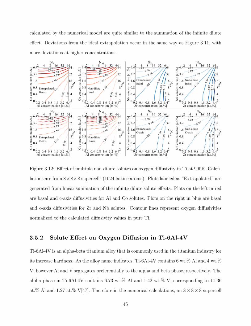
calculated by the numerical model are quite similar to the summation of the infinite dilute
effect. Deviations from the ideal extrapolation occur in the same way as Figure 3.11, with
more deviations at higher concentrations.
2 4 8 16 32 64
2
4
8
16
32
64
NAl
NCo
0.2 0.4 0.8 1.6 3.2 6.4Al concent rat ion [at .%]
0.2
0.4
0.8
1.6
3.2
6.4
Coconcentration[at.%]
0.80
0.90
1.00
1.10
1.201.301.401.501.601.70
NZr
NNb
0.2 0.4 0.8 1.6 3.2 6.4Zr concent rat ion [at .%]
0.2
0.4
0.8
1.6
3.2
6.4
Nbconcentration[at.%] 0.88
0.92
0.96
1.00
1.04
1.08
1.12 1.1
6
2 4 8 16 32 64
2
4
8
16
32
64
0.2 0.4 0.8 1.6 3.2 6.4Al concent rat ion [at .%]
0.2
0.4
0.8
1.6
3.2
6.4
Coconcentration[at.%]
0.901.00
1.10
1.201.30
1.401.501.601.701.801.90
2 4 8 16 32 64
2
4
8
16
32
64
NAl
NCo
0.2 0.4 0.8 1.6 3.2 6.4Zr concent rat ion [at .%]
0.2
0.4
0.8
1.6
3.2
6.4
Nbconcentration[at.%] 0.88
0.92
0.96
1.00
1.04
1.08
1.12
2 4 8 16 32 64
2
4
8
16
32
64
NZr
NNb
0.2 0.4 0.8 1.6 3.2 6.4Zr concent rat ion [at .%]
0.2
0.4
0.8
1.6
3.2
6.4
Nbconcentration[at.%]
0.92
0.96
1.00
1.04
1.08
2 4 8 16 32 64
2
4
8
16
32
64
NZr
NNb
0.2 0.4 0.8 1.6 3.2 6.4Zr concent rat ion [at .%]
0.2
0.4
0.8
1.6
3.2
6.4
Nbconcentration[at.%] 0.88
0.92
0.96
1.00
1.04
1.08
1.12
1.16
2 4 8 16 32 64
2
4
8
16
32
64
NZr
NNb
0.2 0.4 0.8 1.6 3.2 6.4Al concent rat ion [at .%]
0.2
0.4
0.8
1.6
3.2
6.4
Coconcentration[at.%]
0.80
0.90
1.00
1.10
1.201.30
1.401.50
2 4 8 16 32 64
2
4
8
16
32
64
NAl
NCo
ExtrapolatedC-axis
ExtrapolatedBasal
Non-diluteC-axis
Non-diluteBasal
ExtrapolatedC-axis
ExtrapolatedBasal
Non-diluteC-axis
Non-diluteBasal
0.2 0.4 0.8 1.6 3.2 6.4Al concent rat ion [at .%]
0.2
0.4
0.8
1.6
3.2
6.4
Coconcentration[at.%]
0.901.00
1.10
1.201.301.40
1.501.601.70
2 4 8 16 32 64
2
4
8
16
32
64
NAl
NCo
Figure 3.12: Effect of multiple non-dilute solutes on oxygen diffusivity in Ti at 900K. Calcu-
lations are from 8×8×8 supercells (1024 lattice atoms). Plots labeled as “Extrapolated” are
generated from linear summation of the infinite dilute solute effects. Plots on the left in red
are basal and c-axis diffusivities for Al and Co solutes. Plots on the right in blue are basal
and c-axis diffusivities for Zr and Nb solutes. Contour lines represent oxygen diffusivities
normalized to the calculated diffusivity values in pure Ti.
3.5.2 Solute Effect on Oxygen Diffusion in Ti-6Al-4V
Ti-6Al-4V is an alpha-beta titanium alloy that is commonly used in the titanium industry for
its increase hardness. As the alloy name indicates, Ti-6Al-4V contains 6 wt.% Al and 4 wt.%
V; however Al and V segregates preferentially to the alpha and beta phase, respectively. The
alpha phase in Ti-6Al-4V contains 6.73 wt.% Al and 1.42 wt.% V, corresponding to 11.36
at.% Al and 1.27 at.% V[47]. Therefore in the numerical calculations, an 8× 8× 8 supercell
45

(1024 lattice atoms) is used with 116 Al atoms and 13 V atoms. Comparing to oxygen
diffusivity in pure titanium at 900K, this composition of Ti-6Al-4V gives relative oxygen
diffusivities of 0.607 for basal and 0.621 c-axis. These values are calculated from 10000
random distributions of Al and V atoms, giving an estimated error of the mean of less than
1%. These values are close to the approximation of simply adding up the infinite dilute
effects (Table 3.3) of Al and V according to their atomic concentrations (Eqn. (3.7)), giving
0.588 for basal and 0.629 c-axis.
0 0.02 0.04 0.06 0.08Solute Concentration
0.7
0.8
0.9
1.0
1.1
1.2
1.3
1.4
1.5
D /
D0T
i-6A
l-4V
1 8 32 64N
solute
ScMo
0 0.02 0.04 0.06 0.08Solute Concentration
0.7
0.8
0.9
1.0
1.1
1.2
1.3
1.4
1.51 8 32 64
Nsolute
ZrNb
BasalC-axis
Figure 3.13: Effect of non-dilute solute concentrations on oxygen diffusivity in Ti-6Al-4V at
900K. Calculations are from 8 × 8 × 8 supercells (1024 lattice atoms) of Ti-6Al-4V. Please
note that oxygen diffusivities are normalized to the calculated diffusivity values in Ti-6Al-4V.
Error bars represent the standard error of the mean for the diffusivity at each concentration
estimated from 1000 runs. Lines show the extrapolation from the infinite dilute results
(Figure 3.7 and Table 3.3) from pure titanium.
Figure 3.13 shows the effect of adding solutes to the Ti-6Al-4V alloy calculated with
our numerical diffusion method. Up to 64 atoms of Mo, Nb, Sc, or Zr are included in the
46

numerical diffusion model in addition to the 116 Al and 13 V atoms. Diffusion for these
calculations are computed slightly differently from previous solute runs. Since the goal is to
look at the effect of solutes on a specific Ti-alloy, the diffusivity of oxygen is not calculated by
randomizing all the solutes—116 Al, 13 V, and additional solute—and comparing the results
to the Ti-6Al-4V result calculated previously. Instead, for each run, 116 Al and 13 V atoms
are randomly distributed in an 8×8×8 supercell and the diffusivity is calculated for that Ti-
6Al-4V distribution. Then with the same Al and V solute distribution, the additional solute
is randomly placed in the supercell. The diffusivity for this new Ti-6Al-4V-X distribution is
normalized by the diffusivity of the Ti-6Al-4V distribution calculated in the previous step.
1000 of these runs for each additional solute is calculated and shown in Figure 3.13. The
extrapolated lines on the plot are from the infinite dilute effects for pure titanium, applied
on top of the Ti-6Al-4V diffusivity. The estimated error of the mean for these runs are
larger than that of the single solute type calculations (Figure 3.11). This is to be expected,
since with three different types of solutes, there are many more different possible solute
configurations and in turn more transition energies possibilities for the diffusing oxygen.
The pure titanium infinite dilute effect extrapolation does surprisingly well when applied to
the four additional solutes in Ti-6Al-4V, though deviations do show up at lower additional
solute concentrations. This shows that the infinite dilute solute effects can be very useful at
predicting the changes in oxygen diffusivity at various alloy compositions.
3.6 Approximation Errors in the Diffusion Model
Several approximations have been used to calculate the effect of solutes on the diffusion of
oxygen through titanium. In this section we will quantify the effect of the KRA approxima-
tion and the nearest neighbor interaction approximation.
Table 3.5 compares the kinetically resolved activation barrier (KRA) approximation used
in the diffusion model and first principles NEB calculations of the diffusion barriers for Al and
47

Table 3.5: Comparison between transition barriers for oxygen in pure titanium, modeledusing KRA from solute interactions, and direct DFT calculation with NEB. Values are givenin units of eV.
No Solute Al KRA Al NEB Sc KRA Sc NEBo→h 2.04 1.91 1.81 2.08 2.05o→c 2.16 2.00 1.88 2.42 2.37h→o 0.85 0.98 0.87 0.81 0.78h→c 0.94 0.98 0.89 1.13 1.10c→o 0.28 0.33 0.15 0.19 0.13c→h 0.24 0.23 0.09 0.18 0.14
Table 3.6: Table of oxygen-solute interaction energies for octahedral neighbors beyond thefirst nearest neighbor. Values are given in units of eV, positive values indicate repulsiveinteraction, while negative values indicate an attractive interaction.
Na+0.026+0.068
K-0.014+0.106
Rb+0.006+124
Cs+0.011+0.132
Mg-0.007+0.021
Ca-0.013+0.056
Sr+0.002+0.084
Ba+0.016+0.109
Sc-0.007+0.020
Y-0.004+0.041
La+0.027+0.072
Ti+0.00+0.00
Zr-0.005+0.009
Hf+0.001+0.003
V+0.004-0.009
Nb-0.005-0.006
Ta+0.001-0.014
Cr-0.024-0.026
Mo-0.070-0.037
W-0.014-0.026
Mn+0.027+0.054
Tc+0.003-0.007
Re-0.000-0.022
Fe+0.000-0.014
Ru+0.015+0.067
Os+0.012-007
Co-0.016-0.016
Rh+0.014+0.040
Ir-0.019+0.012
Ni+0.025+0.040
Pd+0.001+0.054
Pt+0.010+0.043
Cu+0.014+0.041
Ag-0.012+0.045
Au-0.004+0.042
Zn+0.015+0.028
Cd-0.009+0.025
Hg-0.006+0.029
Ga+0.038+0.029
Al+0.032+0.016
In+0.012+0.017
Tl+0.010+0.022
Si+0.076+0.051
Ge+0.072+0.051
Sn+0.042+0.030
Pb+0.034+0.030
3
4
5
6
1 2
3 4 5 6 7 8 9 10 11 12
13 14Solute
octahedral 2nnoctahedral 3nn
Sc. The transitions calculated are ones where both the starting and ending configurations
neighbor the same solute atom. It is at these transition saddle points that we expect the KRA
approximation to be at its worst. For all transition barriers the KRA approximation differs
from the direct calculation by less than 0.18eV. There is also a systematic overestimation
of the barrier height by KRA as compared to the direct results. These errors affect the
amount of time oxygen spends around the solute, however the kinetics of sampled jumps
are much less affected due to the systematic nature of the errors. When we replace those
specific transitions in our diffusion model with those that were calculated directly with DFT
(with all remaining barriers approximated by KRA), we obtain diffusivity results that differ
by less than 0.1% when compared with the model with all KRA barriers.
48
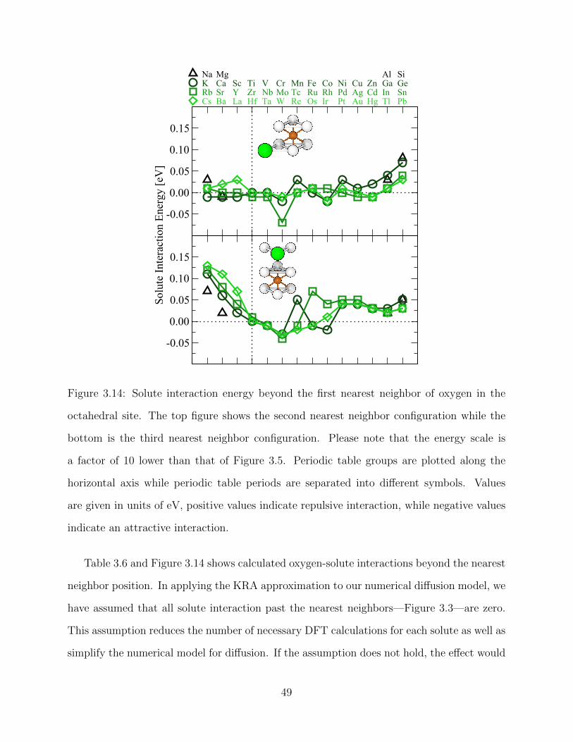
NaKRbCs
MgCaSrBa
ScYLa
TiZrHf
VNbTa
CrMoW
MnTcRe
FeRuOs
CoRhIr
NiPdPt
CuAgAu
ZnCdHg
AlGaInTl
SiGeSnPb
-0.05
0.00
0.05
0.10
0.15
SoluteInteractionEnergy[eV]
-0.05
0.00
0.05
0.10
0.15
Figure 3.14: Solute interaction energy beyond the first nearest neighbor of oxygen in the
octahedral site. The top figure shows the second nearest neighbor configuration while the
bottom is the third nearest neighbor configuration. Please note that the energy scale is
a factor of 10 lower than that of Figure 3.5. Periodic table groups are plotted along the
horizontal axis while periodic table periods are separated into different symbols. Values
are given in units of eV, positive values indicate repulsive interaction, while negative values
indicate an attractive interaction.
Table 3.6 and Figure 3.14 shows calculated oxygen-solute interactions beyond the nearest
neighbor position. In applying the KRA approximation to our numerical diffusion model, we
have assumed that all solute interaction past the nearest neighbors—Figure 3.3—are zero.
This assumption reduces the number of necessary DFT calculations for each solute as well as
simplify the numerical model for diffusion. If the assumption does not hold, the effect would
49

be an artificially reduced solute interaction radius with oxygen in the numerical diffusion
model. However, we see in Figure 3.14 that the second and third nearest neighbor solute
interactions with oxygen in the octahedral site are not large in magnitude. In most cases the
interaction energy is more than a factor of 10 lower than the nearest neighbor interaction
(Figure 3.5a). This is due to the increased oxygen-solute distance of the octahedral second
and third neighbor sites, 3.61A and 3.88A, respectively. These distances are much more
than the five nearest neighbors we did consider (Figure 3.3), which all have oxygen-solute
distances of ∼2A. The fourth nearest neighbor for the octahedral site is 4.64A away from
the oxygen and is expected to be interact much less than the second and third neighbors.
The error bars in Figure 3.7 show the effect of including second and third nearest neighbor
interactions into our numerical diffusion model. The effect on diffusion from almost all
solutes changed by less than 4 (units of percentage change in diffusivity per atomic percent
solute concentration) with the addition of second and third nearest octahedral neighbor
interactions. The single exception is Mo, which decreases oxygen diffusivity by approximately
10 after accounting for the second and third neighbor interactions. The reason for this
decrease is due to the negative interaction between oxygen and Mo at the second and third
neighbor positions, as can be seen in Figure 3.14. A negative interaction means that oxygen
at the octahedral ground-state is attracted to Mo solutes, and this attraction traps diffusing
oxygen atoms and lead to lowered diffusivity.
3.7 Summary
We have used ab initio calculations to predict the effect of solutes on oxygen diffusion in α-
titanium. Oxygen interstitial site energy changes in the presence of 45 solutes are calculated
with DFT. The effect of solutes on oxygen diffusion barriers in titanium is modeled with
the kinetically resolved activation barrier approximation from the site energy changes. A
numerical diffusion framework is constructed to calculate the change in oxygen diffusivity
50

at various solute concentrations and the infinite dilute solute effect is extracted. Trends
in the oxygen diffusion change correlates with changes in sign of the solute interaction.
The diffusion model give predictions for non-dilute solute concentration effects as well as
diffusivity predictions for specific titanium alloys. The developed diffusion framework allows
the future study of the effect of various solute distributions on oxygen diffusion.
51
CHAPTER 4
OXYGEN DIFFUSION IN HCPMETALS
4.1 Computational Methods
First-principles calculations are performed with vasp[28, 48, 49, 29], a plane-wave density-
functional theory (DFT) code. Oxygen and each of the 15 HCP elements are treated
with the projector augmented-wave (PAW) method[32] with the PBE exchange-correlation
functional[22]. Table 4.1 lists the valence configuration for all pseudopotentials used. We
choose the PAW method in order to obtain the all-electron charge densities for analysis with
improved Bader integration[50]. We use a single oxygen atom with 96 lattice atoms in a
4× 4× 3 HCP supercell with 4× 4× 4 k-point mesh. A plane-wave cutoff of 400eV is used
for all metals and is converged to 0.3meV/atom. The k-point mesh with Methfessel-Paxton
smearing of 0.2eV is converged to 1meV/atom. To determine energy barriers for interstitial
hops, we use the climbing-image nudged elastic band[23, 34] method with one intermediate
image and constant cell shape. Since we only consider simple transitions involving only a
single interstitial atom, one image is sufficient to determine the transition saddle point. With
the climbing-image modification, the force on the image along the path is negated, while
components perpendicular to the path are unchanged; the image relaxed to an extremum
where the forces are less than 5meV/A, and restoring forces confirm that this extremum is
a first-order saddle point.
52

Table 4.1: PAW pseudopotential valence configurations for the 15 HCP elements and oxygen.
Valence ConfigurationsO 2s22p4 Ru 4d75s1
Be 2s2 Sc 3s23p63d24s1
Cd 4d105s2 Tc 4p64d55s2
Co 3d74s2 Ti 3p63d24s2
Hf 5p65d26s2 Tl 5d106s26p1
Mg 3s2 Y 4s24p64d15s2
Os 5d66s2 Zn 3d104s2
Re 5d56s2 Zr 4s24p64d35s1
4.2 Oxygen Interstitial Sites in HCP Lattices
Figure 4.1 shows the location for various observed oxygen interstitial defects in the HCP lat-
tice as well as their Wyckoff positions[5]. For HCP systems the most commonly discussed in-
terstitials are the octahedral and tetrahedral, with six and four equivalent neighboring atoms,
respectively. Recently, it has been found through DFT calculations that oxygen in titanium
occupies the hexahedral site[1] rather than tetrahedral and oxygen is also metastable at the
non–basal crowdion site in titanium[41]. The hexahedral site is five-fold coordinated with
three nearest lattice atom neighbors in the basal plane and two further neighbors directly
above and below. The non-basal crowdion site is six-fold coordinated with two significantly
displaced lattice atom neighbors and four further neighbors. While all HCP systems contain
the octahedral site, the other listed interstitial sites are not present in all systems. Indeed,
the tetrahedral and hexahedral sites are mutually exclusive for all 15 systems studied. It
should also be mentioned that for all systems with stable tetrahedral sites, the oxygen does
not reside at the perfect tetrahedral positions as shown in Figure 4.1. Rather, oxygen dis-
place away from the basal face of the tetrahedral site for Co, Os, Re, Ru, and Tc; and
displace towards the basal face for the remaining tetrahedral systems. Other high symmetry
sites, such as the basal crowdion were not found to be metastable for oxygen in any of the
15 HCP elements studied.
53

Site Wyckoff pos. Site Wyckoff pos.
octahedral 2a (0, 0, 0) hexahedral 2d (23, 1
3, 1
4)
tetrahedral 4f (23, 1
3, 1
8) crowdion 6g (1
2, 0, 0)
Figure 4.1: Wyckoff positions and unit cell locations for oxygen interstitial sites in HCP
systems. On the left: octahedral (orange) and tetrahedral (blue). On the right: hexahedral
(blue) and crowdion (black).
4.3 Oxygen Transition Pathways in HCP Lattices
Figure 4.2 shows all possible transitions between interstitial sites in HCP systems. Since
tetrahedral and hexahedral sites do not coexist in any system, no H–T transition networks are
shown. For networks which contain the tetrahedral site, the T–T transition is also included
in the figure. The T–T transition is a local jump between neighboring tetrahedral sites
and allows c-axis mobility in those single networks. Depending on the available interstitials
for each system, octahedral sites may be connected to six distinct tetrahedral sites, six
hexahedral sites, six crowdion sites, and two other octahedrals. Tetrahedral sites connect to
three octahedral sites, three crowdion sites, and the neighboring tetrahedral site. Hexahedral
sites connect to six octahedral sites and six crowdion sites. Crowdion sites connect to two
octahedral sites, two tetrahedral sites, and two hexahedral sites. The complete oxygen
54

diffusion network for each specific HCP system is the summation of all the networks in
Figure 4.2 which contain interstitial sites available to that system.
O-OO-H
H-C O-C
O-T
T-C
Figure 4.2: Connectivity network for transitions between interstitial sites in the HCP lattice.
Note that the O–T and T–C networks also include T–T transitions between neighboring
tetrahedral sites. White spheres represent the HCP lattice atoms, orange for octahedral,
blue for tetrahedral and hexahedral, and black for crowdion interstitial sites.
The analytical diffusion equations for each of the individual diffusion networks (Fig-
ure 4.2) are given in Table 4.2. The diffusion equations are given in terms of λij, the
transition rate for oxygen jumping from site i to site j. At temperature T , λij is equal to
the Arrhenius equation: λij = νij exp(−Eij/kBT ), where νij is the attempt prefactor for the
transition and Eij is the energy barrier relative to the site energy of site i. Please note that
since these equations are for the transition networks independent of one another, compar-
isons can only be made after applying the appropriate fractional occupancy for sites in the
network.
55
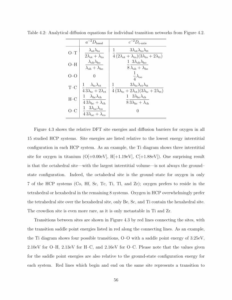
Table 4.2: Analytical diffusion equations for individual transition networks from Figure 4.2.
a−2Dbasal c−2Dc-axis
O–Tλotλto
2λot + λto
1
4
3λotλtoλtt
(2λot + λto)(3λto + 2λtt)
O–Hλohλho
λoh + λho
1
8
3λohλho
λoh + λho
O–O 01
4λoo
T–C1
4
λtcλct
3λtc + 2λct
1
4
3λtcλctλtt
(3λtc + 2λct)(3λtc + 2λtt)
H–C1
4
λhcλch
3λhc + λch
1
8
3λhcλch
3λhc + λch
O–C1
4
3λocλco
3λoc + λco
0
Figure 4.3 shows the relative DFT site energies and diffusion barriers for oxygen in all
15 studied HCP systems. Site energies are listed relative to the lowest energy interstitial
configuration in each HCP system. As an example, the Ti diagram shows three interstitial
site for oxygen in titanium (O[+0.00eV], H[+1.19eV], C[+1.88eV]). One surprising result
is that the octahedral site—with the largest interstitial volume—is not always the ground–
state configuration. Indeed, the octahedral site is the ground–state for oxygen in only
7 of the HCP systems (Co, Hf, Sc, Tc, Ti, Tl, and Zr); oxygen prefers to reside in the
tetrahedral or hexahedral in the remaining 8 systems. Oxygen in HCP overwhelmingly prefer
the tetrahedral site over the hexahedral site, only Be, Sc, and Ti contain the hexahedral site.
The crowdion site is even more rare, as it is only metastable in Ti and Zr.
Transitions between sites are shown in Figure 4.3 by red lines connecting the sites, with
the transition saddle point energies listed in red along the connecting lines. As an example,
the Ti diagram shows four possible transitions, O–O with a saddle point energy of 3.25eV,
2.10eV for O–H, 2.13eV for H–C, and 2.16eV for O–C. Please note that the values given
for the saddle point energies are also relative to the ground-state configuration energy for
each system. Red lines which begin and end on the same site represents a transition to
56

a neighboring site of the same type (O–O, T–T). Refer to Figure 4.2 to visualize how the
different transitions appear in the HCP lattice. Tetrahedral sites for Hf, Tl, Y, and Zr are
labeled as T* and are referred to as shallow tetrahedrals due to the very low T–T barrier
(<0.03eV) connecting neighboring tetrahedral sites. This shallow barrier may allow the
formation of a pseudo-hexahedral configuration at high temperatures.
O - OctahedralT - TetrahedralH - HexahedralC - Crowdion T* - Shallow Tetrahedral
O T
0
1
2
Zinc
O T
0
1
2
Ruthenium
O T
0
1
2
Magnesium
O H
0
1
2
3
Beryllium
O H
0
1
2
Scandium
O H C
0
1
2
3
Titanium
O T*
0
1
2
3
Hafnium
O T
0
1
2
Cobalt
O T
0
1
2
Cadmium
O T
0
1
2
Rhenium
O T
0
1
2
Osmium
O T*
0
1
2
Yttrium
O T* C
0
1
2
3
Zirconium
O T*
0
1
2
Thallium
O T
0
1
2
Technetium
0.00 0.00
0.00 0.00
0.00 0.00
0.00 0.00
0.00 0.00
0.00
0.00 0.00
0.00 0.00
0.57 0.440.20
1.36
0.230.27
1.53
0.04
0.24
1.19
0.89
0.910.37
0.03 0.17
1.060.62
0.17
0.740.41
0.15
1.031.29
1.02
1.071.40
0.92
1.000.68
0.10
1.41
2.101.66
2.83
1.65
1.210.79
0.02
1.49
1.00
3.14
1.97
0.94
1.51
0.990.69
1.011.160.80
0.320.210.04
2.94
1.95
0.91
3.25
2.16
1.891.82
2.132.01
Figure 4.3: Oxygen interstitial site energies and diffusion barriers in all 15 HCP elements.
Energy in units of eV is represented on the vertical axis, while possible metastable inter-
stitial sites for each element is placed on the horizontal axis. The elements are grouped by
commonalities of interstitial stability; on the right, elements have the octahedral interstitial
site as the ground-state configuration, while elements on the left do not. The dotted line
separate elements with hexahedral sites (Be, Sc, and Ti) versus elements with tetrahedral
sites. The dashed line separate elements with crowdion sites (Ti and Zr) versus elements
that do not. Relative site energies are given in black, while possible transitions between sites
are connected by red lines with the respective saddle point energies given in red, also rela-
tive to the ground-state configuration energy. Some tetrahedral sites are labeled as shallow
tetrahedral (T*) due to the low T–T transition barrier in that element.
Few ab initio calculations for oxygen in HCP are available in the literature. One compar-
57

ison is done by Middleburgh and Grimes[51], where they used DFT to study various defects
and their diffusion in beryllium. They found that oxygen relaxes to the hexahedral site from
the tetrahedral and that the octahedral site is 1.38 eV higher in energy than the hexahedral
(our calculations give 1.53 eV higher). They also found the O–O barrier to be 2.71 eV and
the O–H barrier to be 1.63 eV, both energies are relative to the hexahedral site energy.
Our calculations give 2.83 eV for the O–O barrier and 1.65 eV for the O–H barrier, again
relative to the hexahedral site energy. Another DFT study done by Zhang et al.[52] gives
very similar results, with the octahedral being 1.50 eV higher than hexahedral, O–O barrier
to be 2.76 eV, and O–H barrier at 1.63 eV. The excellent agreement with two separate DFT
calculations for oxygen diffusion in beryllium serves as validation of our methodology for the
other HCP systems.
4.4 Oxygen Diffusion Through HCP Metals
As before, we have derived full analytical diffusion equations for oxygen in each HCP system.
The diffusion equations are given in terms of λij, the transition rate for oxygen jumping
from site i to site j. At temperature T , λij is equal to the Arrhenius equation: λij =
νij exp(−Eij/kBT ), where Eij is the energy barrier and νij is the attempt prefactor for the
transition. Please note that Eij in this equation is relative to the site energy of site i. For
different HCP systems, the diffusion equations in the basal and c-axis directions are distinct
according to the set of interstitial sites possible ({O, T}, {O, H}, {O, T, C}, {O, H, C}).
For systems with only octahedral and tetrahedral sites (Cd, Co, Hf, Mg, Os, Re, Ru, Tc,
Tl, Y, and Zn):
Dbasal = a2
[λotλto
2λot + λto
]Dc =
1
4c2
[λot(3λtoλtt + 3λooλto + 2λooλtt)
(2λot + λto)(3λto + 2λtt)
](4.1)
58
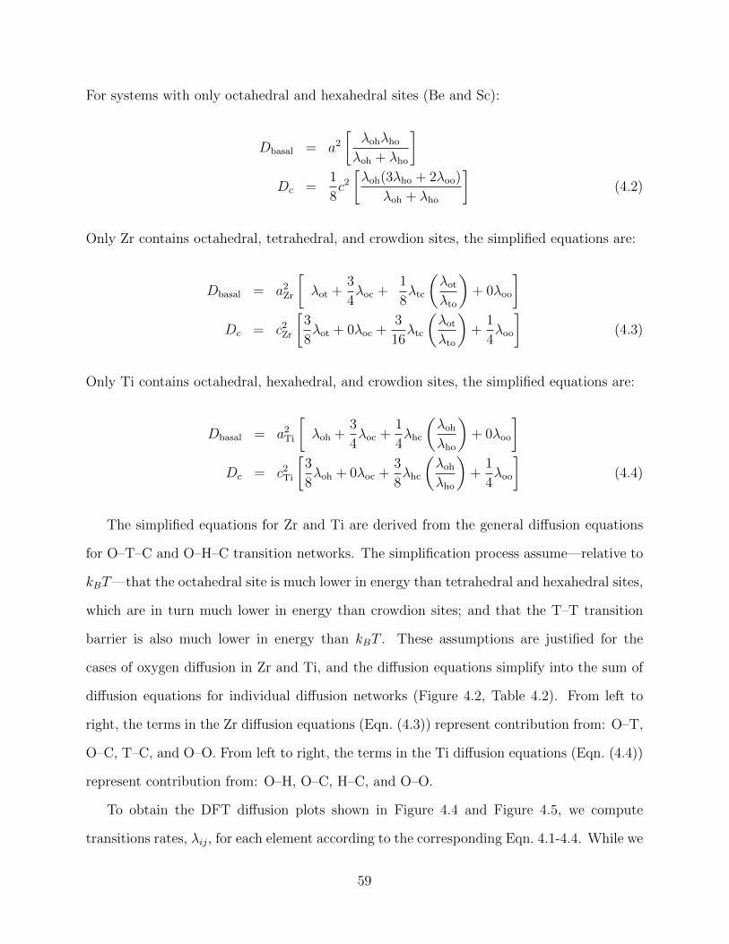
For systems with only octahedral and hexahedral sites (Be and Sc):
Dbasal = a2
[λohλho
λoh + λho
]Dc =
1
8c2
[λoh(3λho + 2λoo)
λoh + λho
](4.2)
Only Zr contains octahedral, tetrahedral, and crowdion sites, the simplified equations are:
Dbasal = a2Zr
[λot +
3
4λoc +
1
8λtc
(λot
λto
)+ 0λoo
]Dc = c2
Zr
[3
8λot + 0λoc +
3
16λtc
(λot
λto
)+
1
4λoo
](4.3)
Only Ti contains octahedral, hexahedral, and crowdion sites, the simplified equations are:
Dbasal = a2Ti
[λoh +
3
4λoc +
1
4λhc
(λoh
λho
)+ 0λoo
]Dc = c2
Ti
[3
8λoh + 0λoc +
3
8λhc
(λoh
λho
)+
1
4λoo
](4.4)
The simplified equations for Zr and Ti are derived from the general diffusion equations
for O–T–C and O–H–C transition networks. The simplification process assume—relative to
kBT—that the octahedral site is much lower in energy than tetrahedral and hexahedral sites,
which are in turn much lower in energy than crowdion sites; and that the T–T transition
barrier is also much lower in energy than kBT . These assumptions are justified for the
cases of oxygen diffusion in Zr and Ti, and the diffusion equations simplify into the sum of
diffusion equations for individual diffusion networks (Figure 4.2, Table 4.2). From left to
right, the terms in the Zr diffusion equations (Eqn. (4.3)) represent contribution from: O–T,
O–C, T–C, and O–O. From left to right, the terms in the Ti diffusion equations (Eqn. (4.4))
represent contribution from: O–H, O–C, H–C, and O–O.
To obtain the DFT diffusion plots shown in Figure 4.4 and Figure 4.5, we compute
transitions rates, λij, for each element according to the corresponding Eqn. 4.1-4.4. While we
59

Table 4.3: Debye temperature[53, 54, 55] (TD), Debye frequency (νD), and attempt frequency(ν = νD(mmatrix/moxygen)1/2) for HCP elements, not including Ti. νD is used to approximatethe attempt frequency in diffusion calculations.
Be Cd Co Hf Mg Os ReTD [K] 1463 214 453 251 387 477 405νD [THz] 30.48 4.45 9.44 5.23 8.05 9.94 8.44ν [THz] 22.88 11.81 18.12 17.47 9.92 34.27 28.79
Ru Sc Tc Tl Y Zn ZrTD [K] 499 362 454 79 257 327 296νD [THz] 10.40 7.55 9.46 1.65 5.35 6.81 6.16ν [THz] 26.14 12.65 23.41 5.90 12.62 13.77 14.72
have the DFT energy barriers, Eij, from Figure 4.3, we still require the attempt frequencies
νij. For the case of oxygen in titanium[41], this was done by calculating the Vineyard attempt
frequency[33] for each individual transition. In this work, we approximate all the attempt
frequencies for oxygen in a single HCP system as ν, calculated from
ν
νD
=
√mmatrix
moxygen
, (4.5)
where mmatrix is the mass of the HCP matrix atom, moxygen is the mass of oxygen, and
νD is the Debye frequency for each HCP element. The Debye frequency νD is computed
from the element’s Debye temperature[53, 54, 55] (TD) with the relation: TD=νD(h/kB).
This approximation is reasonable because the lattice vibration frequency is generally the
same order of magnitude as the diffusion attempt frequency, which should scale with the
mass ratios of the diffusant and matrix. For Ti, TD = 425K (νD = 8.85THz), giving an
attempt frequency of ν = 15.31THz. This value is comparable to the previously reported
DFT attempt frequencies (Table 2.1), all of which—with one exception—were above 10THz.
The Debye temperatures, Debye frequencies, and the approximate attempt frequencies for
the 14 HCP elements (excluding Ti) are listed in Table 4.3.
60
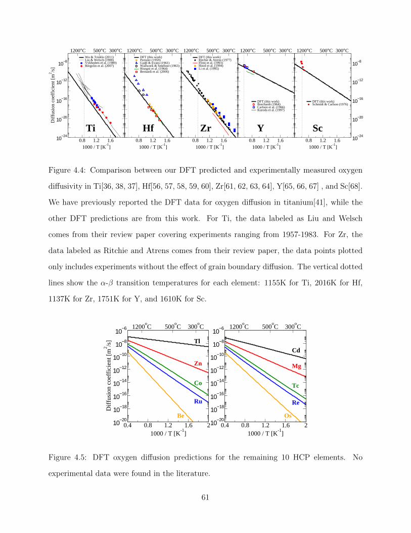
0.8 1.2 1.61000 / T [K
-1]
10−24
10−20
10−16
10−12
10−8
Dif
fusi
on c
oeff
icie
nt [
m2 /s
]1200°C 500°C 300°C
Wu & Trinkle (2011)Liu & Welsch (1988)Vykhodets et al. (1989)Bregolin et al. (2007)
0.8 1.2 1.61000 / T [K
-1]
1200°C 500°C 300°CDFT (this work)Pemsler (1959)Gadd & Evans (1961)Wallwork & Smeltzer (1963)Bisogni et al. (1964)Bernardi et al. (2006)
0.8 1.2 1.61000 / T [K
-1]
1200°C 500°C 300°CDFT (this work)Ritchie & Atrens (1977)Flinn et al. (1993)Hood et al. (1994)Li et al. (1995)
0.8 1.2 1.61000 / T [K
-1]
1200°C 500°C 300°C
DFT (this work)Borchardt (1964)Carlson et al. (1966)Kuroda et al. (1997)
0.8 1.2 1.61000 / T [K
-1]
10−24
10−20
10−16
10−12
10−8
1200°C 500°C 300°C
DFT (this work)Schmidt & Carlson (1976)
Ti Hf Zr Y Sc
Figure 4.4: Comparison between our DFT predicted and experimentally measured oxygen
diffusivity in Ti[36, 38, 37], Hf[56, 57, 58, 59, 60], Zr[61, 62, 63, 64], Y[65, 66, 67] , and Sc[68].
We have previously reported the DFT data for oxygen diffusion in titanium[41], while the
other DFT predictions are from this work. For Ti, the data labeled as Liu and Welsch
comes from their review paper covering experiments ranging from 1957-1983. For Zr, the
data labeled as Ritchie and Atrens comes from their review paper, the data points plotted
only includes experiments without the effect of grain boundary diffusion. The vertical dotted
lines show the α-β transition temperatures for each element: 1155K for Ti, 2016K for Hf,
1137K for Zr, 1751K for Y, and 1610K for Sc.
0.4 0.8 1.2 1.6 21000 / T [K
-1]
10−20
10−18
10−16
10−14
10−12
10−10
10−8
10−6
Dif
fusi
on c
oeff
icie
nt [
m2 /s
]
1200oC 500
oC 300
oC
0.4 0.8 1.2 1.6 21000 / T [K
-1]
10−20
10−18
10−16
10−14
10−12
10−10
10−8
10−6 1200oC 500
oC 300
oC
Cd
Mg
Tc
Re
Os
Tl
Zn
Co
Ru
Be
Figure 4.5: DFT oxygen diffusion predictions for the remaining 10 HCP elements. No
experimental data were found in the literature.
61

Figure 4.4 shows comparisons between oxygen diffusion coefficients calculated from DFT
and experimentally reported diffusion data for Ti, Hf, Zr, Y, and Sc. Oxygen diffusion
in Ti, Hf, and Zr make up the vast majority of available experimental literature, with
fewer reports found for Y and Sc. The overall diffusion energy slope for Ti, Hf, Zr, and
Y match very well between the DFT diffusion curves and the experimental data. The
absolute DFT diffusivity values for these four elements also lie within the experimental
spread. Our predicted slope for oxygen diffusion in scandium disagree significantly with the
single experiment available[68]. The DFT diffusion barriers that we calculated for scandium
are not substantially different when compared to those of the other 14 HCP elements, and
no indication from the calculations that there are different mechanisms at work for oxygen in
scandium. It is possible that the discrepancy is due to the experiment’s attempt to measure
the diffusivity near the α-β transition temperature for Sc. Figure 4.5 shows the predicted
DFT oxygen diffusivity curves for the remaining 10 HCP elements. We were not able to find
any experimental results in the literature for oxygen diffusion in these elements.
4.5 Trends in Oxygen Energetics in HCP Metals
Figure 4.6 plots various system properties, with and without the oxygen present, against the
stability of oxygen interstitial sites in the HCP elements. Figure 4.6a shows the correlation
between the system lattice parameter and the c/a ratio, Figure 4.6b shows the correlation
between the Bader volume and the Bader charge of the oxygen, and Figure 4.6c shows the
correlation between the local potential energy and the charge density at empty interstitial
sites. None of these comparisons reveal any simple correlation for whether the oxygen octa-
hedral site is ground-state or not. Though there is a weak separation in the Bader analysis
plot (Figure 4.6b), with the lower-right being predominantly octahedral stable (orange) and
the upper-left being tetrahedral/hexahedral stable (blue). This corresponds to a preference
by oxygen to occupy a smaller Bader volume and hold more Bader charge.
62

Be
Cd
Mg
OsRe
RuY
Zn
CoHf
ScTc
Ti TlZr
2.0 2.5 3.0 3.5 4.0Lattice Constant, a [Å]
1.5
1.6
1.7
1.8
1.9
c/a
Rat
io
Be
Cd
Mg
OsRe Ru
Y
Zn
CoHfSc
TcTi
Tl
Zr
-0.15 -0.10 -0.05 0.00 0.05Bader Charge Difference (o - t) [e]
0.90
0.95
1.00
1.05
1.10
Bad
er V
olum
e R
atio
(o
/ t)
Co
Hf
Sc
Tc
Ti
Tl
ZrBe
CdMg
OsReRu
Y
Zn
-0.15 -0.10 -0.05 0.00Charge Density Difference (o - t)
0.5
1.0
1.5
2.0
2.5
Loca
l Pot
entia
l Diff
eren
ce (
o -
t) [e
V]
Cd
Co
Mg
Os
Re
Ru
Tc
Zn
Hf
TlY
ZrBe
Sc Ti
0.00 0.02 0.04Charge Density Difference (h - t)
-0.8
-0.6
-0.4
-0.2
0.0
Loca
l Pot
entia
l Diff
eren
ce (
h -
t) [e
V]
Be
CdMg
Os
ReRu
Y
Zn
Co
Hf
Sc Tc
Ti
Tl
Zr
1 2 3 4 5 6 7 8 9Valence
-2
-1
0
1
2
Rel
ativ
e S
ite E
nerg
y (o
- t)
[eV
]
Be
CdMg
Os
ReRu
Y
Zn
Co
Hf
Sc Tc
Ti
Tl
Zr
500 600 700 800 900 1000First Ionization Energy [kJ/mol]
-2
-1
0
1
2
Rel
ativ
e S
ite E
nerg
y (o
- t)
[eV
]
(a) (b)
(d)
(c)
(e) (f)
Figure 4.6: Correlation with respect to oxygen energetics between the 15 HCP elements.
(a) Comparison of the lattice constant and the c/a ratio for the HCP elements. The dot-
ted line represents the ideal HCP c/a = 1.633. (b) Comparison of the Bader volume ratio
and the Bader charge difference for the oxygen interstitial at the octahedral site and the
tetrahedral/hexahedral site. Comparison of the local potential energy difference and the
charge density difference at the octahedral site and the tetrahedral/hexahedral site (c), and
at the hexahedral site and the tetrahedral site (d). Correlation between the octahedral–
tetrahedral/hexahedral energy difference and the metal valence (e) and the first ionization
energy (f). In (a)-(c) and (e)-(f), the HCP elements are colored according to the oxygen
ground-state configuration in that element, orange for octahedral site and blue for tetrahe-
dral/hexahedral site. In (d), the HCP elements are colored according to the stability of the
oxygen tetrahedral in that element, black for tetrahedral stable, red for hexahedral stable,
and green for shallow tetrahedral stable.
Figure 4.6d shows the comparison between the local potential energy and the charge
63

density at the tetrahedral and hexahedral positions in an empty HCP lattice. There is a
distinct separation in the lower-left for stable tetrahedral (black) sites and the upper-right for
stable hexahedral (red) and shallow tetrahedral (green) sites. In Figure 4.6e-f the numerical
energy difference between oxygen at the octahedral site and the tetrahedral/hexahedral site
is compared to the metal valence and the first ionization energy, respectively. Both show
weak trends, the octahedral is most stable at mid-valence with the ground-state shifting
to tetrahedral/hexahedral at low and high valence. Elements with higher first ionization
energies seem to favor tetrahedral/hexahedral sites while the octahedral site becomes more
stable for elements with lower first ionization energies.
While no general trends for oxygen diffusion extend across all 15 HCP elements in Fig-
ure 4.3, much more similarities exist between elements at close proximity on the periodic
table.
O T*
0
1
2
3
Hafnium
0.00
0.91
3.14
1.97
0.94
O T* C
0
1
2
3
Zirconium
0.00
0.89
2.94
1.95
0.91
1.891.82
O H C
0
1
2
3
Titanium
0.00
1.19
3.25
2.16
2.132.01
Figure 4.7: Comparison of oxygen interstitial energetics for Ti, Zr, and Hf.
Figure 4.7 shows that the titanium group—Ti, Zr, and Hf—all exhibit a high barrier for
oxygen transition between octahedral sites (∼3 eV), and comparable activation energies for
diffusion (∼2 eV). Ti prefers the hexahedral site over the tetrahedral, with both Zr and Hf
preferring the very similar shallow tetrahedral site. Ti and Zr are also the only two HCP
elements which contains a stable non-basal crowdion site for oxygen.
64

O T*
0
1
2
Yttrium
0.000.04
1.21
0.79
0.02
O H
0
1
2
Scandium
0.000.24
1.49
1.00
Figure 4.8: Comparison of oxygen interstitial energetics for Sc and Y.
Figure 4.8 shows that the scandium group—Sc and Y—possess qualitatively similar site
stabilities, with Sc preferring the hexahedral site while Y prefers a shallow tetrahedral. The
magnitudes of their diffusion barriers are also similar, both O–O barriers are about 1.5 times
that of their respective O–H and O–T barriers.
O T
0
1
2
Ruthenium
0.00
0.44
1.031.29
1.02
O T
0
1
2
Rhenium
0.000.23
1.07
1.40
0.92
O T
0
1
2
Osmium
0.00
1.36
1.41
2.10
1.66
O T
0
1
2
Technetium
0.000.17
1.011.16
0.80
Figure 4.9: Comparison of oxygen interstitial energetics for Tc, Ru, Re, and Os.
Figure 4.9 shows that Tc, Ru, Re, and Os—in the middle of the transition metals—all
appear qualitatively the same, having relatively high T–T barriers and low O–O barriers.
With the O–O barrier lower than the O–T barrier for these four elements, high diffusion
anisotropy will emerge between the basal and c-axis directions.
65

10−24
10−20
10−16
10−12
10−8
Dif
fusi
on c
oeff
icie
nt [
m2 /s
]
1200oC 500
oC 300
oC
10−24
10−20
10−16
10−12
10−8
Dif
fusi
on c
oeff
icie
nt [
m2 /s
]
1200oC 500
oC 300
oC
0.4 0.8 1.2 1.6 21000 / T [K
-1]
10−24
10−20
10−16
10−12
10−8 1200oC 500
oC 300
oC
0.4 0.8 1.2 1.6 21000 / T [K
-1]
10−24
10−20
10−16
10−12
10−81200oC 500
oC 300
oC
Os Re
TcRu
Dc-axis
Dbasal
Dc-axis
Dc-axisD
c-axis
Dbasal
Dbasal
Dbasal
Figure 4.10: Comparison between c-axis and basal diffusion for Os, Re, Ru, and Tc.
Figure 4.10 shows the anisotropy between the c-axis and basal diffusion coefficients for
Os, Re, Ru, and Tc. At 1000K, Dc-axis / Dbasal is approximately 5 for Tc, 10 for Ru, 30 for
Re, and 1000 for Os; this anisotropy grows larger at lower temperatures. In contrast, the
anisotropy between c-axis and basal oxygen diffusion for all other HCP systems is less than
a factor of two over the entire temperature range.
O T
0
1
2
Zinc
0.00
0.57
1.06
0.62
0.17
O T
0
1
2
Cadmium
0.000.27
0.74
0.410.15
Figure 4.11: Comparison of oxygen interstitial energetics for Zn and Cd.
66

Figure 4.11 shows that the zinc group—Zn and Cd—again give very similar oxygen
energetics. With full d-shells, Zn and Cd both possess unusually high c/a ratios (c/a > 1.8);
a possible reason explaining why they both have the tetrahedral site as the ground-state. In
terms of diffusion barriers, both have very similar T–T barriers with similar ratios between
O–O and O–T barriers.
O T
0
1
2
Magnesium
0.000.20
1.000.68
0.10
O H
0
1
2
3
Beryllium
0.00
1.53
2.83
1.65
O T
0
1
2
Cobalt
0.000.37
1.51
0.990.69
O T*
0
1
2
Thallium
0.00 0.03
0.320.210.04
Figure 4.12: Comparison of oxygen interstitial energetics for Be, Mg, Co, and Tl.
Finally, Figure 4.12 shows the remaining four HCP elements—Be, Mg, Co, and Tl—
which are not easily classified together with any other element. Though Be and Mg are in
the same group, beryllium’s light mass and small lattice makes it quite different from all
other HCP elements. Mg and Co both have c/a ratios close to ideal (1.633) and have oxygen
diffusion barriers that somewhat resemble Zn and Cd. Thallium has the lowest oxygen
diffusion barrier out of all HCP elements and is the only element not from the left side of
the periodic table to have either a T* or H site.
4.6 Summary
We have used ab initio calculation to determine oxygen diffusion pathways in 15 HCP metals
as well as oxygen diffusion barriers within each element. A variety of different interstitial
site combinations were discovered for oxygen in these HCP elements. Analytical diffusion
equations have been derived for each unique diffusion network. Combined with calculated
67

DFT diffusion barriers, we predict diffusivity curves for oxygen in all 15 HCP elements,
which match well to available experimental data. A surprising result is the discovery that
oxygen does not prefer the large octahedral interstitial site in 8 of the 15 HCP elements.
This preference of the tetrahedral/hexahedral site is counterintuitive and an explanation has
not been found after simple analysis of the HCP lattice characteristics and the electronic
environment of the oxygen interstitials. The large variety of interstitial sites as well as their
stability found within these 15 HCP elements should serve as a reminder that surprises can
be hidden in very simple and well studied systems.
68

CHAPTER 5
CONCLUSION AND FUTUREWORK
5.1 Summary of Results
The work presented improves understanding for the behavior of oxygen in HCP metals. DFT
calculations allow accurate predictions of interstitial energetics and transition barriers. A
systematic framework is developed which models transition barrier changes by taking DFT
interstitial-solute interaction energies to make prediction on changes in the diffusivity.
Oxygen diffusion in titanium is studied in detail using DFT. In the α-titanium lattice
three interstitial sites are available for oxygen, the octahedral, hexahedral, and non-basal
crowdion. While the hexahedral (+1.19eV) and crowdion (+1.88eV) are much higher in
energy compared to the ground-state octahedral site, calculated transition barriers between
the three sites show that all networks contribute to oxygen diffusion. Analytical diffusion
equations for oxygen are derived and the predicted diffusion coefficients from DFT barriers
match well to experimental diffusion measurements.
Solute interaction energies with oxygen in the titanium lattice are calculated for 45
substitutional solutes across the periodic table. The interaction energies changes drastically
depending on which interstitial site the oxygen occupies next to the solute. Almost no
solutes possess an attractive interaction towards the octahedral ground-state site. The KRA
approximation is used to link the effect solutes have on site energies to their effect on
transition barriers between sites. A numerical diffusion model is used to make predictions
for how oxygen diffusivity changes due to these transition barrier changes for individual
solutes, non-dilute concentrations, as well as multiple solute species.
69
Oxygen diffusion in 15 HCP metals is investigated with DFT. Four interstitial sites—
octahedral, tetrahedral, hexahedral, and crowdion—are occupied by oxygen in various combi-
nations in these different systems. Surprisingly, while all systems possess a stable octahedral,
it is only the ground-state site for 7 of the 15 HCP metals despite having the largest intersti-
tial volume. A comparison of the octahedral stability against various system properties only
show limited correlation and this issue is currently unsolved. Analytical diffusion equations
for oxygen in all HCP systems are derived and match well to available experimental diffusion
measurements.
5.2 Future Work
The current results for non-dilute solute concentrations are for random solute distributions.
This would not be the case for alloys with significant solute-solute interactions. Nor does
it take into account the possibility of engineering specific solute distributions. To make
accurate predictions for these cases, further DFT calculations for solute-solute interaction
energies are needed to be able to statistically generate expected solute separations. It is also
necessary to couple the results from the numerical diffusion model to higher length scale
continuum methods such as phase field simulations.
The systematic database for solute interactions with oxygen in titanium as well as the
unexpected results obtained for oxygen in HCP motivates the extension of the computational
methodology to other systems. This includes the energetics and transitions for various light
element interstitials in other simple crystal lattices, such as FCC and BCC. These studies
will provide a more fundamental understanding of interstitial transport in metals. While
the more comprehensive systematic solute studies may provide insight for defect segregation
and precipitation growth.
70
REFERENCES
[1] R. G. Hennig, D. R. Trinkle, J. Bouchet, S. G. Srinivasan, R. C. Albers, and J. W.Wilkins, Impurities block the alpha to omega martensitic transformation in Titanium,Nat. Mater. 4, 129–133 (2005).
[2] A. Borghesi, B. Pivac, A. Sassella, and A. Stella, Oxygen precipitation in silicon, J.Appl. Phys. 77, 4169 (1995).
[3] J. P. Hirth, Effects of hydrogen on the properties of iron and steel, Metall. Trans. A11, 861–890 (1980).
[4] M. Wasz, F. Brotzen, R. McLellan, and A. Griffin, Effect of oxygen and hydrogen onmechanical properties of commercial purity titanium, International Materials Reviews41, 1–12 (1996).
[5] T. Hahn, editor, International Tables for Crystallography, volume A, Dordrecht: KluwerAcademic, 5th edition, 2002.
[6] G. Lutjering and J. C. Williams, Titanium, Engineering Materials and Processes,Springer Berlin Heidelberg, second edition, 2007.
[7] H. Conrad, Effect of interstitial solutes on the strength and ductility of titanium, Prog.Mat. Sci. 26, 123–403 (1981).
[8] J. L. Murray and H. A. Wriedt, The O-Ti (Oxygen-Titanium) system, Journal of PhaseEquilibria 8, 148–165 (1987).
[9] M. Long and H. Rack, Titanium alloys in total joint replacement—a materials scienceperspective, Biomaterials 19, 1621–1639 (1998).
[10] R. Boyer, An overview on the use of titanium in the aerospace industry, MaterialsScience and Engineering: A 213, 103–114 (1996).
[11] S. Yamaguchi, Interstitial Order-Disorder Transformation in the Ti-O Solid Solution.I. Ordered Arrangement of Oxygen, J. Phys. Soc. Jpn. 27, 155–163 (1969).
[12] T. Tsuji, Thermochemistry of IVA transition metal-oxygen solid solutions, J Nucl.Mater. 247, 63–71 (1997).
71

[13] V. B. Vykhodets, T. E. Kurennykh, and A. Y. Fishman, Identification of HeterogeneousState and Trajectories of Interstitials in the Titanium-Oxygen System Using PreciseDiffusion Experiment, Defect and Diffusion Forum 143-147, 79–84 (1997).
[14] A. V. Ruban, V. I. Baykov, B. Johansson, V. V. Dmitriev, and M. S. Blanter, Oxygenand nitrogen interstitial ordering in hcp Ti, Zr, and Hf: An ab initio study, Phys. Rev.B 82, 134110 (2010).
[15] J. M. Macak, H. Tsuchiya, L. Taveira, S. Aldabergerova, and P. Schmuki, Smoothanodic TiO2 nanotubes, P. Angew. Chem., Int. Ed. 44, 7463–7465 (2005).
[16] V. B. Vykhodets and T. Y. Kurennyk, The Mechanism of Oxygen Jumps during Dif-fusion in α-Ti, Phys. Met. Metall. 78, 325–329 (1994).
[17] Y. A. Bertin, J. Parisot, and J. L. Gacougnolle., Modele atomique de diffusion del’oxygene dans le titane α, J. Less-Common Met. 69, 121–138 (1980).
[18] W. Kohn and L. J. Sham, Self-consistent equations including exchange and correlationeffects, Phys. Rev. 140, A1133–1138 (1965).
[19] P. Hohenberg and W. Kohn, Inhomogeneous Electron Gas, Phys. Rev. 136, 864–871(1964).
[20] D. M. Ceperley and B. J. Alder, Ground state of the electron gas by a stochasticmethod, Phys. Rev. Lett. 45, 566–569 (1980).
[21] J. P. Perdew and Y. Wang, Accurate and simple analytic representation of the electron-gas correlation energy, Phys. Rev. B 45, 13244–13249 (1992).
[22] J. P. Perdew, K. Burke, and M. Ernzerhof, Generalized Gradient Approximation MadeSimple, Phys. Rev. Lett. 77, 3865–3868 (1996).
[23] G. Mills and H. Jonsson, Quantum and thermal effects in H2 dissociative adsorption:Evaluation of free energy barriers in multidimensional quantum systems, Phys. Rev.Lett. 72(7), 1124–1127 (Feb 1994).
[24] U. Landman and M. F. Shlesinger, Stochastic theory of multistate diffusion in perfectand defective systems. I. Mathematical formalism, Phys. Rev. B 19, 6207–6219 (1979).
[25] U. Landman and M. F. Shlesinger, Stochastic theory of multistate diffusion in perfectand defective systems. II. Case studies, Phys. Rev. B 19, 6220–6237 (1979).
[26] Allnatt and Lidiard, Atomic Transport in Solids, Cambridge University Press, Cam-bridge, 1993.
[27] A. V. der Ven, G. Ceder, M. Asta, and P. D. Tepesch, First-principles theory of ionicdiffusion with nondilute carriers, Phys. Rev. B 64, 184307 (2001).
[28] G. Kresse and J. Hafner, Ab initio molecular dynamics for liquid metals, Phys. Rev. B47, 558–561 (1993).
72

[29] G. Kresse and J. Furthmuller, Efficient iterative schemes for ab initio total-energycalculations using a plane-wave basis set, Phys. Rev. B 54, 11169–11186 (1996).
[30] D. Vanderbilt, Soft self-consistent pseudopotentials in a generalized eigenvalue formal-ism, Phys. Rev. B 41, 7892–7895 (1990).
[31] G. Kresse and J. Hafner, Norm-conserving and ultrasoft pseudopotentials for first-rowand transition elements, J. Phys. Condens. Matter 6, 8245–8257 (1994).
[32] G. Kresse and D. Joubert, From ultrasoft pseudopotentials to the projector augmented-wave method, Phys. Rev. B 59, 1758–1775 (1999).
[33] G. H. Vineyard, Frequency factors and isotope effects in solid state rate processes, J.Phys. Chem. Solids 3, 121–127 (1957).
[34] G. Henkelman, B. Uberuaga, and H. Jonsson, A climbing image nudged elastic bandmethod for finding saddle points and minimum energy paths, J. Chem. Phys. 113, 9901(2000).
[35] I. Syozi, Statistics of Kagome Lattice, Prog. Theor. Phys. 6, 306 (1951).
[36] Z. Liu and G. Welsch, Literature Survey on Diffusivities of Oxygen, Aluminum, andVanadium in Alpha Titanium, Beta Titanium, and in Rutile, Metall. Mater. Trans. A19, 1121–1125 (1988).
[37] F. L. Bregolin, M. Behar, and F. Dyment, Diffusion study of 18O implanted into α-Tiusing the nuclear resonance technique, Appl. Phys. A 86, 481–484 (2007).
[38] V. B. Vykhodets, S. M. Klostman, T. Y. Kurennyk, A. D. Levin, and V. A. Pavlov,Oxygen diffusion in alpha-Ti: Temperature-dependence of oxygen diffusion-coefficients,Phys. Met. Metall. 68, 94 (1989).
[39] A. Einstein, Uber die von der molekularkinetischen Theorie der Warme geforderteBewegung von in ruhenden Flussigkeiten suspendierten Teilchen, Annalen der Physik322, 549–560 (1905).
[40] M. von Smoluchowski, Zur kinetischen Theorie der Brownschen Molekularbewegungund der Suspensionen, Annalen der Physik 326, 756–780 (1906).
[41] H. H. Wu and D. R. Trinkle, Direct Diffusion through Interpenetrating Networks:Oxygen in Titanium, Phys. Rev. Lett. 107, 045504 (2011).
[42] I. Menzies and K. Strafford, A kinetic and morphological study of the oxidation ofTi-Cr alloys in CO2 at 1000 ◦C, Corrosion Science 7, 23 (1967).
[43] A. M. Chaze and C. Coddet, Influence of alloying elements on the dissolution of oxygenin the metallic phase during the oxidation of titanium alloys, Journal of MaterialsScience 22(4), 1206 (1987).
73
[44] D. Vojtech, B. Bartova, and T. Kubatk, High temperature oxidation of titanium–siliconalloys, Materials Science and Engineering: A 361, 50–57 (2003).
[45] V. Vykhodets, S. Klotsman, T. Kurennykh, and A. Levin, Diffusion of oxygen intitanium-aluminium and titanium-zirconium solid solutions, Phys. Met. Metall. 68,145 (1989).
[46] B. Predel, Landolt-Bornstein, New Series, IV/5, Phase Equilibria, Crystallographicand Thermodynamic Data of Binary Alloys, volume 5A–5J, Springer-Verlag, Berlin,1991–1998.
[47] J. Elmer, T. Palmer, S. Babu, and E. Specht, In situ observations of lattice expansionand transformation rates of α and β phases in Ti–6Al–4V, Materials Science andEngineering: A 391, 104–113 (2005).
[48] G. Kresse and J. Hafner., Ab initio molecular-dynamics simulation of the liquid-metal-amorphous-semiconductor transition in germanium, Phys. Rev. B 49, 14251 (1994).
[49] G. Kresse and J. Furthmuller, Efficiency of ab-initio total energy calculations for metalsand semiconductors using a plane-wave basis set, Comput. Mat. Sci. 6, 15 (1996).
[50] M. Yu and D. R. Trinkle, Accurate and efficient algorithm for Bader charge integration,J. Chem. Phys. 134, 064111 (2011).
[51] S. Middleburgh and R. Grimes, Defects and transport processes in beryllium, ActaMaterialia 59, 7095–7103 (2011).
[52] P. Zhang, J. Zhao, and B. Wen, Retention and diffusion of H, He, O, C impurities inBe, J. Nucl. Mater. 423, 164–169 (2012).
[53] D. Singh and Y. P. Varshni, Debye temperatures for hexagonal crystals, Phys. Rev. B24, 4340–4347 (1981).
[54] C. Pantea, I. Stroe, H. Ledbetter, J. Betts, Y. Zhao, L. Daemen, H. Cynn, andA. Migliori, Osmium’s Debye temperature, J. Phys. Chem. Solids 69, 211–213 (2008).
[55] A. F. Guillermet and G. Grimvall, Thermodynamic properties of technetium, J. Less-Common Met. 147, 195–211 (1989).
[56] J. Pemsler, Diffusion of Oxygen in Hafnium, J. Electrochem. Soc. 106, 1067–1068(1959).
[57] J. Gadd and E. Evans, High Temperature Scaling of Hafnium in Air, Corrosion 17,109 (1961).
[58] G. R. Wallwork and W. W. Smeltzer, The Diffusion of Oxygen in Hafnium, J. Elec-trochem. Soc. 110, 943–944 (1963).
[59] E. Bisogni, G. Mah, and C. Wert, Diffusion of gases in special interstitial sites inhafnium, J. Less-Common Met. 7, 197–204 (1964).
74

[60] F. Bernardi, M. Behar, A. R. abd J.H.R. dos Santos, and F. Dyment, Diffusion studyof 18O implanted into α-Hf using the nuclear resonance technique, Appl. Phys. A 83,37–40 (2006).
[61] I. Ritchie and A. Atrens, The diffusion of oxygen in α-zirconium, J. Nucl. Mater. 67,254–265 (1977).
[62] B. J. Flinn, C.-S. Zhang, and P. R. Norton, Oxygen diffusion along the [0001] axis inZr(0001), Phys. Rev. B 47, 16499–16505 (1993).
[63] G. Hood, H. Zou, S. Herbert, R. Schultz, H. Nakajima, and J. Jackman, Oxygendiffusion in α-Zr single crystals, J. Nucl. Mater. 210, 1–5 (1994).
[64] B. Li, A. Allnatt, C.-S. Zhang, and P. Norton, Model and theory for the determination ofdiffusion coefficients by Auger electron spectroscopy measurements and an applicationto oxygen diffusion along the [0001] and [1010] axes in single crystal zirconium, Surf.Sci. 330, 276–288 (1995).
[65] H. Borchardt, On the oxidation of yttrium, J. Inorg. Nucl. Chem. 26, 711–714 (1964).
[66] O. Carlson, F. Schmidt, and D. Peterson, Electrotransport of interstitial atoms inyttrium, J. Less-Common Met. 10, 1–11 (1966).
[67] K. Kuroda, T. Yoshida, T. Fujisawa, and C. Yamauchi, J. Min. Mater. Process. Inst.JPN 113, 179–184 (1997).
[68] F. Schmidt and O. Carlson, Electrotransport of carbon, nitrogen and oxygen in scan-dium, J. Less-Common Met. 50, 237–244 (1976).
75
Related Documents