Overview on Heat Pump Component Noise and Noise Control ...

3: Overview on Heat Pump Component

Noise and Noise Control Techniques

Sebastian Wagner, Fraunhofer Institute for Building Physics IBP, Stuttgart

Xavier Carniel, CETIM Centre technique des industries mécaniques, Senlis

Jens Rohlfing, Fraunhofer Institute for Building Physics IBP, Stuttgart

Karlheinz Bay, Fraunhofer Institute for Building Physics IBP, Stuttgart

Henrik Hellgren, Chalmers University of Technology, Goteborg

Date: November 2020 Draft Version, Review: 02

2/79

3 Component noise and

noise control techniques

Index

1. Introduction ..................................................................................................................... 4

Fundamentals of noise Control ................................................................................... 5

Description of a heat pump......................................................................................... 5

Component noise ........................................................................................................ 7

Noise analysis approach: acoustic synthesis .............................................................. 7

2. Overview of Components Noise ..................................................................................... 9

The fan ........................................................................................................................ 9

The compressor ........................................................................................................ 22

Secondary sources .................................................................................................... 29

Heat exchangers in interaction with fan ................................................................... 31

3. Fundamentals of Noise Control Techniques ................................................................. 33

Airborne noise .......................................................................................................... 33

3.1.1. Sound Absorption ......................................................................................... 34

3.1.2. Silencers ........................................................................................................ 37

3.1.3. Sound transmission and insulation ............................................................... 39

3.1.4. Active noise control techniques .................................................................... 41

Structure-borne noise................................................................................................ 42

3.2.1. Vibration isolation ........................................................................................ 43

3.2.2. Fluid-borne noise .......................................................................................... 46

3.2.3. Modelling and design of passive isolation systems ...................................... 46

3.2.4. Active vibration control techniques .............................................................. 50

4. Concepts for Component Noise Control ....................................................................... 52

Compressor ............................................................................................................... 52

4.1.1. Passive treatments ......................................................................................... 52

4.1.2. Active vibration control ................................................................................ 57

Fan ............................................................................................................................ 57

4.2.1. Fan noise ....................................................................................................... 57


4.2.3. Active noise control ...................................................................................... 61

Secondary sources .................................................................................................... 62

5. Noise Emissions Paths and Concepts for Noise Control .............................................. 63

Air intake and outlets................................................................................................ 63


3/79



5.1.2. Active noise control ...................................................................................... 64

Casing ....................................................................................................................... 66

5.2.1. Noise insulation ............................................................................................ 66

5.2.2. Retrofit solutions .......................................................................................... 67

Structure-borne noise emissions ............................................................................... 67

5.3.1. Passive vibration isolation mounts ............................................................... 67

5.3.2. Adaptive and active mounts ......................................................................... 68

5.3.3. Mountings, pipes .......................................................................................... 68

6. Effect of Operating Conditions of Heat Pumps on Acoustic Behaviour ...................... 69

7. Placement and Installation ............................................................................................ 70

8. Figures Index ................................................................................................................. 73

9. References ..................................................................................................................... 77

4/79



1. Introduction

The global climate is changing faster than ever, and the European public is more and more

informed and aware of it. The anthropogenic climate change due to the wasteful usage of

fossil fuels is one of the central challenges in the 21st century. In order to assume

responsibility for future generations, it is important to meet this challenge with appropriate

measures and urgency. Energy used for heating and cooling accounts for almost 50 percent

of the EU’s total primary energy demand [1]. Hence, moving towards efficient and

environment-friendly heating systems can significantly reduce primary energy consumption.

In this context, heat pumps have been identified as a key technology, especially heat pumps

using outside air as a heat source. By using green electricity in connection with heat pump

technology, almost zero C02 emissions can be reached [2]. On the other side, when used in

large numbers in urban areas, heat pumps emit a considerable amount of noise. To protect

residents against noise pollution and avoid annoyance, noise emission standards need to be

obeyed. In the Annex 51 Task 1 report, the national laws and regulations regarding noise

protection of some European member states are summarised [3]. Besides general laws and

regulations on noise protection, the Task 1 report also covers regulations which specifically

address noise emissions from heat pumps.

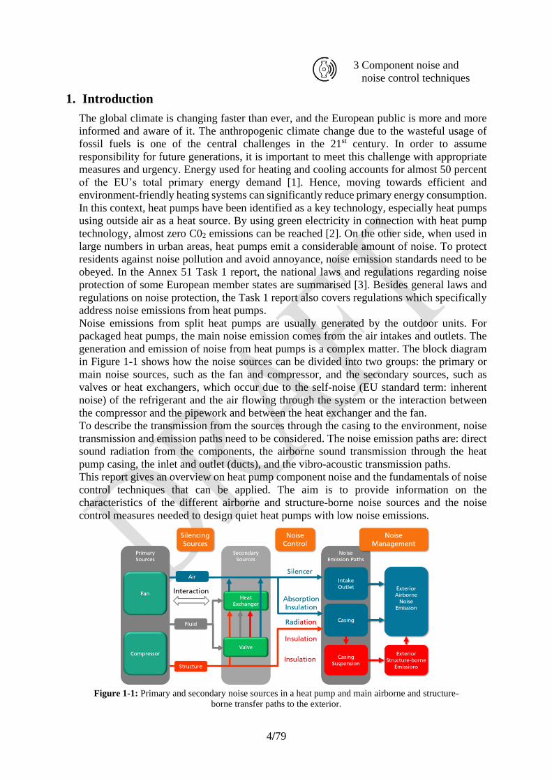
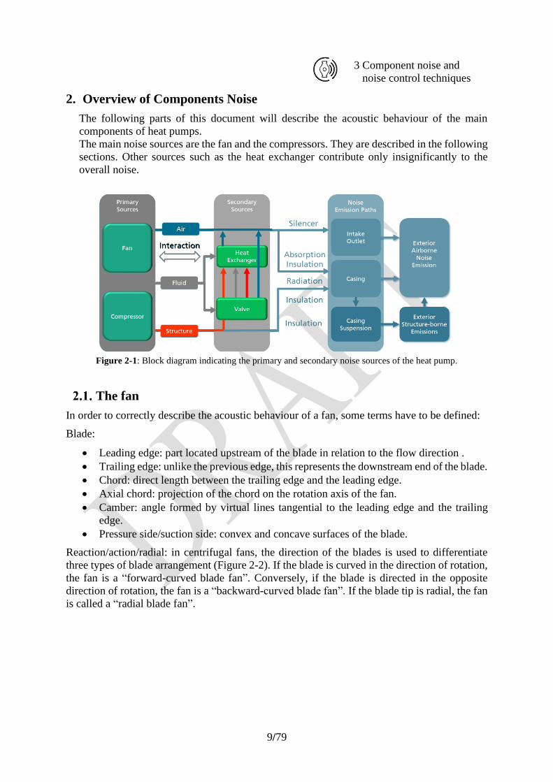
Noise emissions from split heat pumps are usually generated by the outdoor units. For

packaged heat pumps, the main noise emission comes from the air intakes and outlets. The

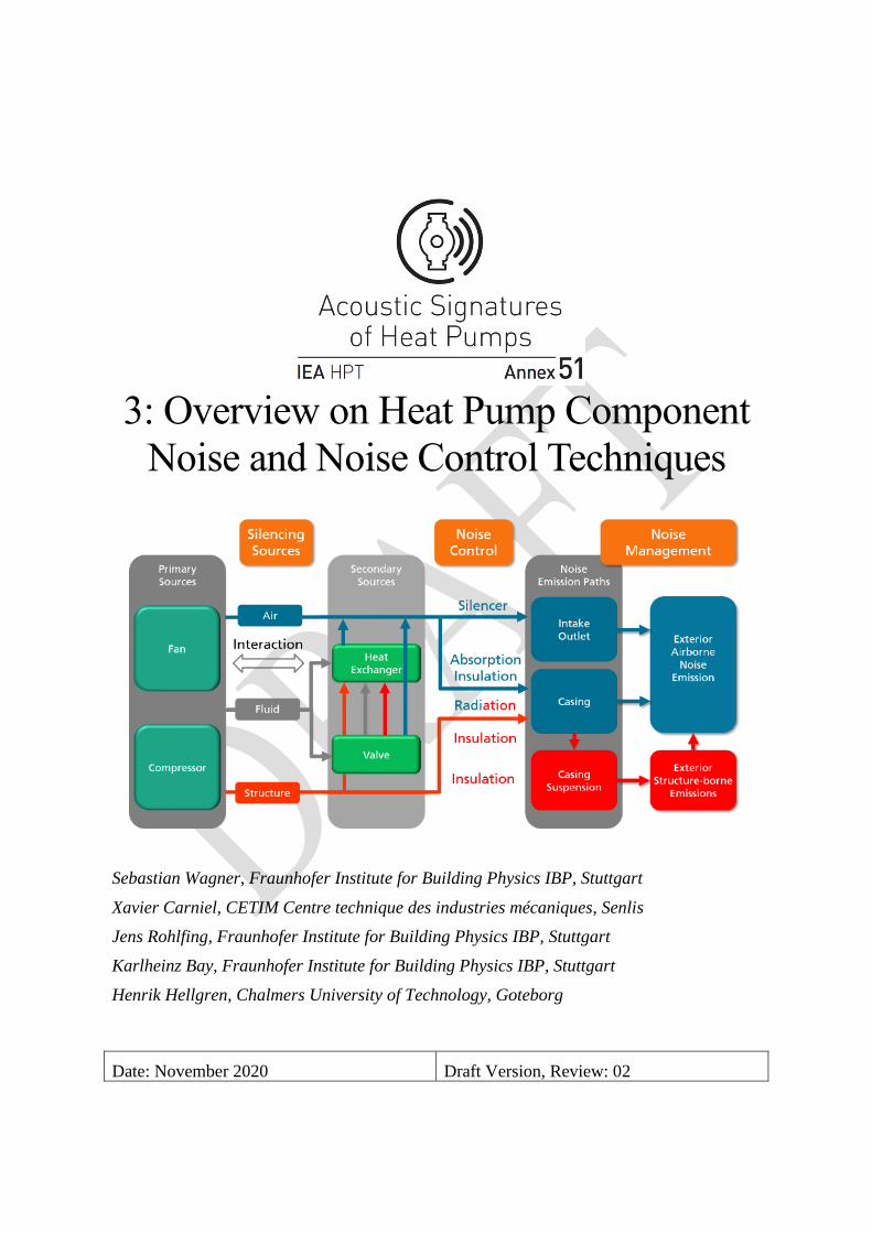
generation and emission of noise from heat pumps is a complex matter. The block diagram

in Figure 1-1 shows how the noise sources can be divided into two groups: the primary or

main noise sources, such as the fan and compressor, and the secondary sources, such as

valves or heat exchangers, which occur due to the self-noise (EU standard term: inherent

noise) of the refrigerant and the air flowing through the system or the interaction between

the compressor and the pipework and between the heat exchanger and the fan.

To describe the transmission from the sources through the casing to the environment, noise

transmission and emission paths need to be considered. The noise emission paths are: direct

sound radiation from the components, the airborne sound transmission through the heat

pump casing, the inlet and outlet (ducts), and the vibro-acoustic transmission paths.

This report gives an overview on heat pump component noise and the fundamentals of noise

control techniques that can be applied. The aim is to provide information on the

characteristics of the different airborne and structure-borne noise sources and the noise

control measures needed to design quiet heat pumps with low noise emissions.

Figure 1-1: Primary and secondary noise sources in a heat pump and main airborne and structure-

borne transfer paths to the exterior.

5/79



Fundamentals of noise Control

Noise can affect physiological and psychological health by generating stress [3]. Hence, direct

consumers and the wider public have an interest in quiet heat pumps. This puts pressure on heat

pump manufacturers to produce heat pumps that are energy-efficient, quiet, and economical at

the same time.

The most efficient method to reduce noise emissions is to suppress the noise generation at the

source. In heat pumps, this can be achieved by using more quiet compressors or fans. The next

best way to reduce emissions is to decouple the main noise source from the rest of the heat

pump. For example, using elastic mounts to fasten the compressor to the heat pump frame can

greatly reduce the vibrational power transmitted into the frame [3]. Any source may transmit

airborne or structure-borne noise via a number of different parallel paths. Hence, the further

away from the sources, the more difficult it is to control noise transmissions efficiently. If noise

control measures at the heat pump are not efficient enough, it may be necessary to protect the

surrounding with additional expensive retrofit solutions such as noise barriers or acoustic

housings (Section 5.2.2).

Classical noise and vibration control measures are usually passive, such as rubber mounts or

mufflers based on porous material. In recent years there have also been developments in the

area of active noise and vibration control, such as active engine mounts. To date, the application

of active noise and vibration control measures is still restricted to a small number of special

applications in the automotive and aerospace industry. Although active solutions are becoming

increasingly accessible, they are currently not used in heat pumps due to their complexity and

relatively high costs.

Description of a heat pump

This section presents several types of heat pumps. The individual steps of the heating process

are briefly discussed. The main task of a heat pump is the transfer of thermal energy (heat) from

an energy source, e.g. ambient air, groundwater, or geothermal resources, to a second medium

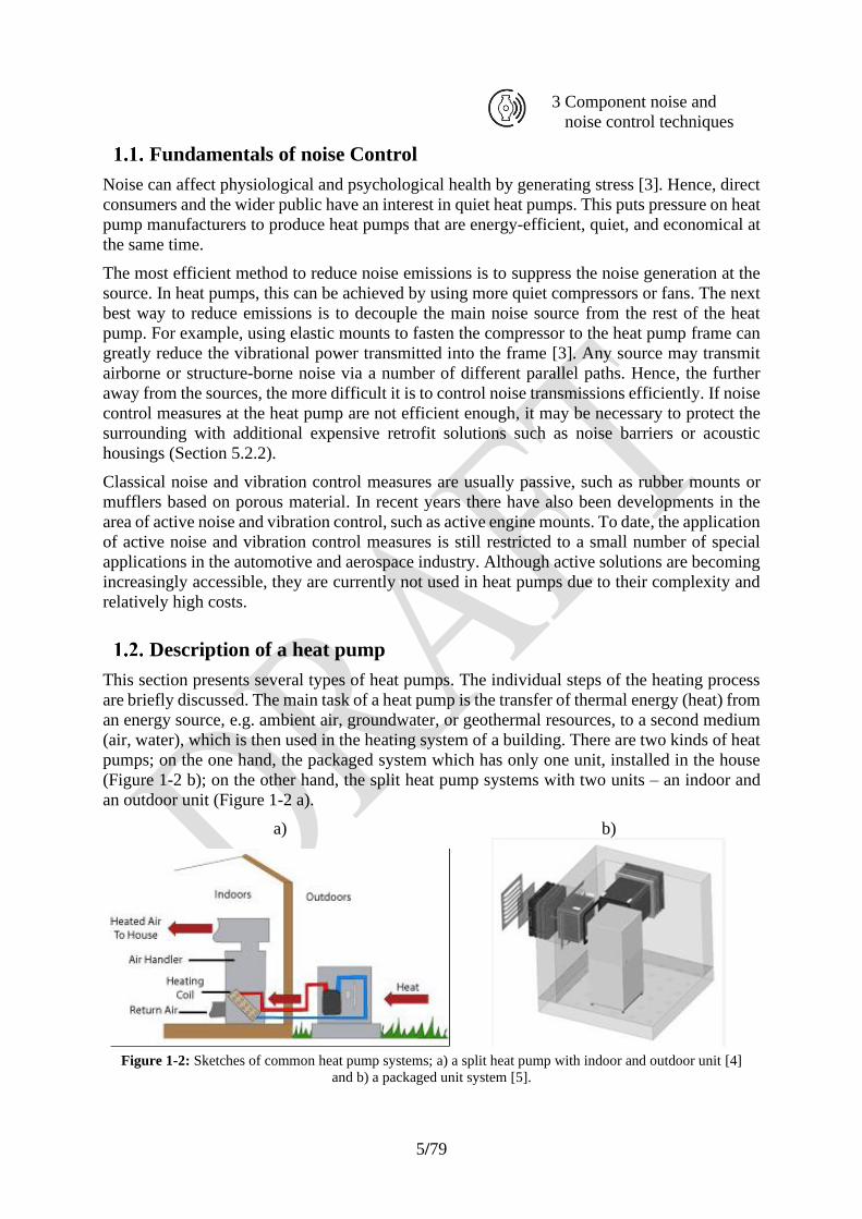
(air, water), which is then used in the heating system of a building. There are two kinds of heat

pumps; on the one hand, the packaged system which has only one unit, installed in the house

(Figure 1-2 b); on the other hand, the split heat pump systems with two units – an indoor and

an outdoor unit (Figure 1-2 a).

a) b)

Figure 1-2: Sketches of common heat pump systems; a) a split heat pump with indoor and outdoor unit [4]

and b) a packaged unit system [5].

6/79



A packaged heat pump allows to have all components (fan, heat exchangers and compressor)

in one cabinet. Air supply and return ducts lead the air through the building’s exterior wall to

the packaged unit, which is often placed in the basement. Such heat pumps have both the heat

transfers to the refrigerant and the heat transfer to the medium of the heating system in the same

unit. As the ducts have a higher flow resistance than the outdoor units, mainly radial fans are

installed in these systems.

Split heat pumps have an indoor and an outdoor unit which are connected through an isolated

conduit. These systems split the heat transfer process into two sections. The first heat transfer

from the air to the refrigerant occurs in the outdoor unit, the second heat transfer from the

refrigerant to the medium of the existing building heating system occurs in the indoor unit.

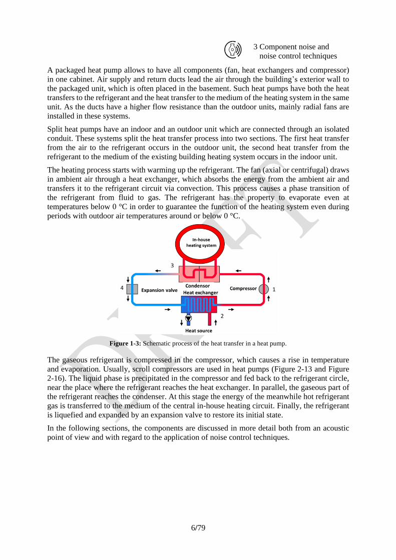
The heating process starts with warming up the refrigerant. The fan (axial or centrifugal) draws

in ambient air through a heat exchanger, which absorbs the energy from the ambient air and

transfers it to the refrigerant circuit via convection. This process causes a phase transition of

the refrigerant from fluid to gas. The refrigerant has the property to evaporate even at

temperatures below 0 °C in order to guarantee the function of the heating system even during

periods with outdoor air temperatures around or below 0 °C.

Figure 1-3: Schematic process of the heat transfer in a heat pump.

The gaseous refrigerant is compressed in the compressor, which causes a rise in temperature

and evaporation. Usually, scroll compressors are used in heat pumps (Figure 2-13 and Figure

2-16). The liquid phase is precipitated in the compressor and fed back to the refrigerant circle,

near the place where the refrigerant reaches the heat exchanger. In parallel, the gaseous part of

the refrigerant reaches the condenser. At this stage the energy of the meanwhile hot refrigerant

gas is transferred to the medium of the central in-house heating circuit. Finally, the refrigerant

is liquefied and expanded by an expansion valve to restore its initial state.

In the following sections, the components are discussed in more detail both from an acoustic

point of view and with regard to the application of noise control techniques.

7/79



Component noise

Any “active” mechanical component may be described as three different sources but also as

transfer functions:

• Airborne source

• Structure-borne source

• Fluid-borne source

The characterisation of airborne sources is well-known and can be achieved on a standalone

mode. To characterise the contribution of structure-borne and fluid-borne noises, the integration

parameters have to be known (characterisation of receiving structure or circuit).

Transfer functions are then to be evaluated according to the vibro-acoustic scheme

(Figure 1-4).

Like heat exchangers, some components can be considered as transfer function and noise

sources: isolation of the noise of other components placed behind them and source due to

circulating fluids inside and outside.

The objective of the noise approach has also to be considered : the characterisation of

components will be different if the objective is to reduce stationary or transient noise, or if noise

level or annoyance is addressed.

Considering all the sources and transfer paths presents an enormous task. The vibro-acoustic

scheme is intended to support the hierarchisation of the contributions. It is the expertise of

acousticians which will help to make the relevant hypothesis.

Noise analysis approach: acoustic synthesis

The noise reduction of heat pumps is complex and far-reaching. Each component can be

considered as a “black box” that emits acoustic and vibrational energy in three forms:

• Airborne noise: acoustic radiation from the component casing (source) and the nearby

structures, propagating in the surrounding air; it is measured using microphones or

sound intensity probes.

• Hydraulic or fluid-borne noise generated in the piping systems and radiated: it originates

in the pressure pulses emitted by the source in the liquid columns of the system (at both

the suction and the discharge of the compressor, for example) and which are broadly

responsible for the noise emission by the piping. It is generally evaluated using flush-

membrane pressure sensors.

• Structure-borne noise: Components generate dynamic forces that are transmitted to the

other components or the heat pump. This structure-borne noise is generally evaluated

by using force sensors, accelerometers, or both.

Each component can include several noise generation mechanisms, and each source can

generate airborne, structure-borne, or fluid-borne noise transmitted in the components, which

have different levels of response to each of these noises. It is evident that, with a view to an

overall reduction of the noise of such a circuit, the main issue is to manage the interaction of

these sources with the components to which they are connected; these components must be

taken into account and identified with respect to the source in order to obtain a “silent system”.

Thus, an elemental vibration and acoustic analysis of such a system is essential, as an overall

approach cannot lead to an optimum solution. However, in general, the supplier of any of the

8/79



(active) components may not necessarily know the other components of a system, and is

therefore not in a position to adapt its source to the actual needs, if necessary. It is common for

a given component, even if it is relatively quiet, to be installed in two different circuits to

generate distinct and potentially damaging vibration and acoustic behaviour. Information

sharing is necessary, particularly regarding source/structure interfacing, and the common work

of suppliers and integrators is consequently essential for the joint execution of an action, for the

improvement of the product, using an acoustic synthesis.

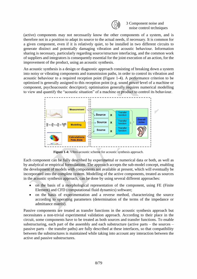
An acoustic synthesis is a design or diagnostic approach consisting of breaking down a system

into noisy or vibrating components and transmission paths, in order to control its vibration and

acoustic behaviour to a required reception point (Figure 1-4). A performance criterion to be

optimized is generally assigned to this reception point (e.g. sound power level of a machine or

component, psychoacoustic descriptor); optimisation generally requires numerical modelling

to view and quantify the “acoustic situation” of a machine or product to control its behaviour.

Figure 1-4: Vibro-acoustic scheme for acoustic synthesis approach.

Each component can be fully described by experimental or numerical data or both, as well as

by analytical or empirical formulations. The approach accepts the sub-model concept, enabling

the development of models with components not available at present, which will eventually be

incorporated into the complete system. Modelling of the active components, treated as sources

in the acoustic synthesis approach, can be done by using several different approaches:

• on the basis of a morphological representation of the component, using FE (Finite

Element) and CFD (computational fluid dynamics) software;

• on the basis of experimentation and a reverse method, characterizing the source

according to operating parameters (determination of the terms of the impedance or

admittance matrix).

Passive components are treated as transfer functions in the acoustic synthesis approach but

necessitates a non-trivial experimental validation approach. According to their place in the

circuit, some components have to be treated as both sources and transfer functions. To enable

substructuring, each part of the assembly and each substructure (active parts – the sources –

passive parts – the transfer paths) are fully described at these interfaces, so that compatibility

between the substructures is maintained while taking into account any interaction between the

active and passive substructures.

9/79



2. Overview of Components Noise

The following parts of this document will describe the acoustic behaviour of the main

components of heat pumps.

The main noise sources are the fan and the compressors. They are described in the following

sections. Other sources such as the heat exchanger contribute only insignificantly to the

overall noise.

Figure 2-1: Block diagram indicating the primary and secondary noise sources of the heat pump.

The fan

In order to correctly describe the acoustic behaviour of a fan, some terms have to be defined:

Blade:

• Leading edge: part located upstream of the blade in relation to the flow direction .

• Trailing edge: unlike the previous edge, this represents the downstream end of the blade.

• Chord: direct length between the trailing edge and the leading edge.

• Axial chord: projection of the chord on the rotation axis of the fan.

• Camber: angle formed by virtual lines tangential to the leading edge and the trailing

edge.

• Pressure side/suction side: convex and concave surfaces of the blade.

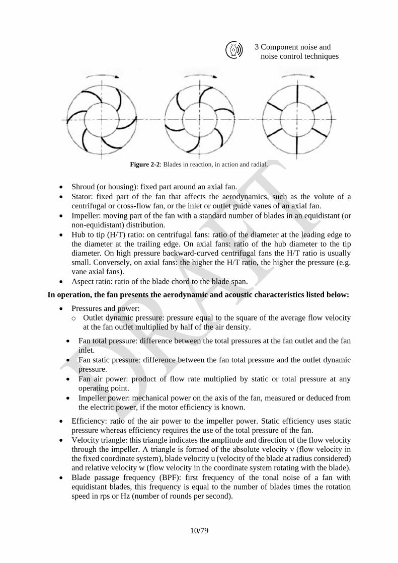
Reaction/action/radial: in centrifugal fans, the direction of the blades is used to differentiate

three types of blade arrangement (Figure 2-2). If the blade is curved in the direction of rotation,

the fan is a “forward-curved blade fan”. Conversely, if the blade is directed in the opposite

direction of rotation, the fan is a “backward-curved blade fan”. If the blade tip is radial, the fan

is called a “radial blade fan”.

10/79



Figure 2-2: Blades in reaction, in action and radial.

• Shroud (or housing): fixed part around an axial fan.

• Stator: fixed part of the fan that affects the aerodynamics, such as the volute of a

centrifugal or cross-flow fan, or the inlet or outlet guide vanes of an axial fan.

• Impeller: moving part of the fan with a standard number of blades in an equidistant (or

non-equidistant) distribution.

• Hub to tip (H/T) ratio: on centrifugal fans: ratio of the diameter at the leading edge to

the diameter at the trailing edge. On axial fans: ratio of the hub diameter to the tip

diameter. On high pressure backward-curved centrifugal fans the H/T ratio is usually

small. Conversely, on axial fans: the higher the H/T ratio, the higher the pressure (e.g.

vane axial fans).

• Aspect ratio: ratio of the blade chord to the blade span.

In operation, the fan presents the aerodynamic and acoustic characteristics listed below:

• Pressures and power:

o Outlet dynamic pressure: pressure equal to the square of the average flow velocity

at the fan outlet multiplied by half of the air density.

• Fan total pressure: difference between the total pressures at the fan outlet and the fan

inlet.

• Fan static pressure: difference between the fan total pressure and the outlet dynamic

pressure.

• Fan air power: product of flow rate multiplied by static or total pressure at any

operating point.

• Impeller power: mechanical power on the axis of the fan, measured or deduced from

the electric power, if the motor efficiency is known.

• Efficiency: ratio of the air power to the impeller power. Static efficiency uses static

pressure whereas efficiency requires the use of the total pressure of the fan.

• Velocity triangle: this triangle indicates the amplitude and direction of the flow velocity

through the impeller. A triangle is formed of the absolute velocity ν (flow velocity in

the fixed coordinate system), blade velocity u (velocity of the blade at radius considered)

and relative velocity w (flow velocity in the coordinate system rotating with the blade).

• Blade passage frequency (BPF): first frequency of the tonal noise of a fan with

equidistant blades, this frequency is equal to the number of blades times the rotation

speed in rps or Hz (number of rounds per second).

11/79



Aerodynamic approach

The fan responds to a flow resistance imposed by the user’s application. The fan must therefore

overcome the pressure drop of the distribution ductwork while providing the flow rate required

by the user.

Concept of pressure loss

The total pressure of a small volume of air in movement is equal to its dynamic pressure plus

its static pressure. The fan provides the necessary energy to compensate for the total air pressure

difference between intake and exhaust of the system in which it is installed in order to make air

move in the system by compensating for air friction losses. This total pressure difference is

called “pressure loss”, Δp. This pressure loss corresponds to the total pressure loss associated

with the resistance of the system at a given air flow rate.

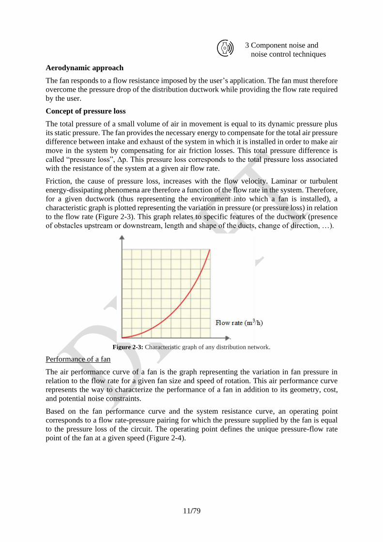
Friction, the cause of pressure loss, increases with the flow velocity. Laminar or turbulent

energy-dissipating phenomena are therefore a function of the flow rate in the system. Therefore,

for a given ductwork (thus representing the environment into which a fan is installed), a

characteristic graph is plotted representing the variation in pressure (or pressure loss) in relation

to the flow rate (Figure 2-3). This graph relates to specific features of the ductwork (presence

of obstacles upstream or downstream, length and shape of the ducts, change of direction, …).

Figure 2-3: Characteristic graph of any distribution network.

Performance of a fan

The air performance curve of a fan is the graph representing the variation in fan pressure in

relation to the flow rate for a given fan size and speed of rotation. This air performance curve

represents the way to characterize the performance of a fan in addition to its geometry, cost,

and potential noise constraints.

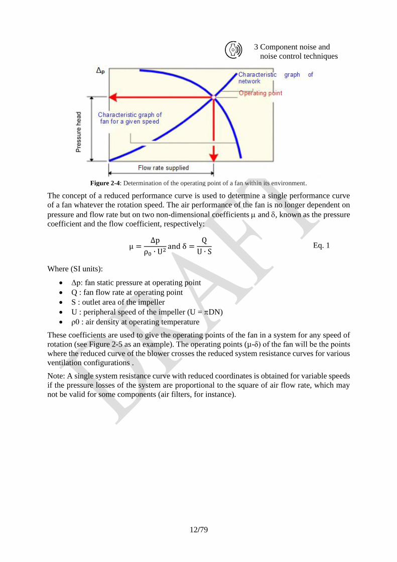
Based on the fan performance curve and the system resistance curve, an operating point

corresponds to a flow rate-pressure pairing for which the pressure supplied by the fan is equal

to the pressure loss of the circuit. The operating point defines the unique pressure-flow rate

point of the fan at a given speed (Figure 2-4).

12/79



Figure 2-4: Determination of the operating point of a fan within its environment.

The concept of a reduced performance curve is used to determine a single performance curve

of a fan whatever the rotation speed. The air performance of the fan is no longer dependent on

pressure and flow rate but on two non-dimensional coefficients and , known as the pressure

coefficient and the flow coefficient, respectively:

μ =∆p

ρ0 ∙ U2and δ =

Q

U ∙ S Eq. 1

Where (SI units):

• Δp: fan static pressure at operating point

• Q : fan flow rate at operating point

• S : outlet area of the impeller

• U : peripheral speed of the impeller (U = DN)

• ρ0 : air density at operating temperature

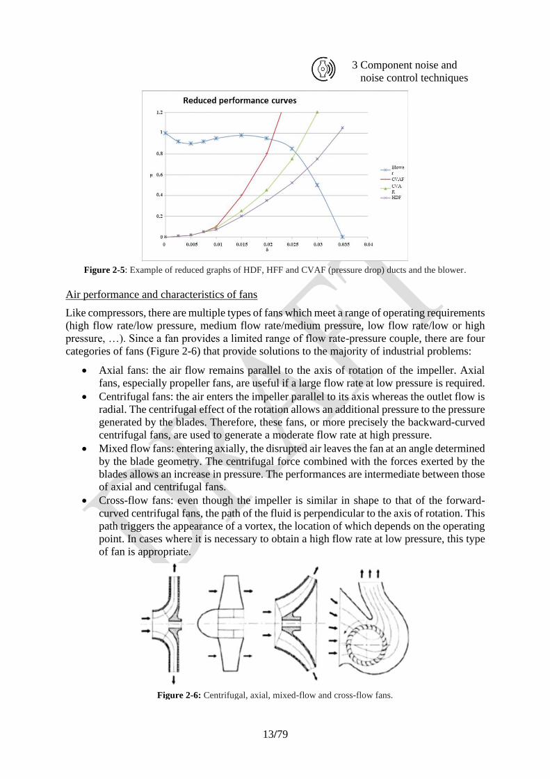
These coefficients are used to give the operating points of the fan in a system for any speed of

rotation (see Figure 2-5 as an example). The operating points (µ-δ) of the fan will be the points

where the reduced curve of the blower crosses the reduced system resistance curves for various

ventilation configurations .

Note: A single system resistance curve with reduced coordinates is obtained for variable speeds

if the pressure losses of the system are proportional to the square of air flow rate, which may

not be valid for some components (air filters, for instance).

13/79



Figure 2-5: Example of reduced graphs of HDF, HFF and CVAF (pressure drop) ducts and the blower.

Air performance and characteristics of fans

Like compressors, there are multiple types of fans which meet a range of operating requirements

(high flow rate/low pressure, medium flow rate/medium pressure, low flow rate/low or high

pressure, …). Since a fan provides a limited range of flow rate-pressure couple, there are four

categories of fans (Figure 2-6) that provide solutions to the majority of industrial problems:

• Axial fans: the air flow remains parallel to the axis of rotation of the impeller. Axial

fans, especially propeller fans, are useful if a large flow rate at low pressure is required.

• Centrifugal fans: the air enters the impeller parallel to its axis whereas the outlet flow is

radial. The centrifugal effect of the rotation allows an additional pressure to the pressure

generated by the blades. Therefore, these fans, or more precisely the backward-curved

centrifugal fans, are used to generate a moderate flow rate at high pressure.

• Mixed flow fans: entering axially, the disrupted air leaves the fan at an angle determined

by the blade geometry. The centrifugal force combined with the forces exerted by the

blades allows an increase in pressure. The performances are intermediate between those

of axial and centrifugal fans.

• Cross-flow fans: even though the impeller is similar in shape to that of the forward-

curved centrifugal fans, the path of the fluid is perpendicular to the axis of rotation. This

path triggers the appearance of a vortex, the location of which depends on the operating

point. In cases where it is necessary to obtain a high flow rate at low pressure, this type

of fan is appropriate.

Figure 2-6: Centrifugal, axial, mixed-flow and cross-flow fans.

14/79



In this section, fans of all types (axial, centrifugal, mixed, and cross-flow) will be investigated

to show the geometrical characteristics and air flow performances as well as their efficiency.

Axial fans

There are three types of axial fans:

• Tubeaxial fans: these fans are composed of a wheel with a medium number of blades

(between 3 and 10) and without outlet guide vanes. The impeller is integrated into a

cylindrical housing with a diameter slightly larger than the impeller. The fan generates

a pressure of no more than 1 kPa and produces a flow rate with optimum efficiency (up

to about 80 %) at three quarters of the maximum flow rate.

• Vaneaxial fans: these fans, consisting of airfoil blades with a hub to tip ratio greater

than 50 %, have outlet guide vanes to make the flow at the fan exit axial in order to

recover some static pressure and increase efficiency compared to a tubeaxial fan with

the same impeller. The fan pressure may reach 3 kPa or even more.

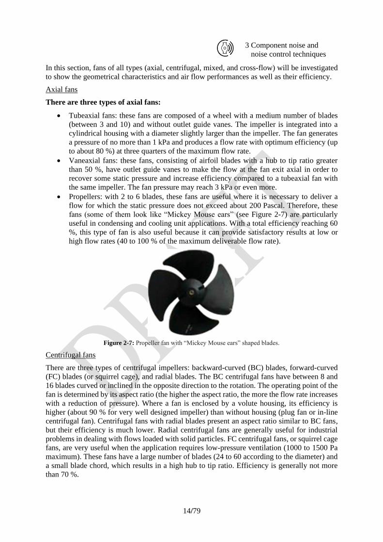
• Propellers: with 2 to 6 blades, these fans are useful where it is necessary to deliver a

flow for which the static pressure does not exceed about 200 Pascal. Therefore, these

fans (some of them look like “Mickey Mouse ears” (see Figure 2-7) are particularly

useful in condensing and cooling unit applications. With a total efficiency reaching 60

%, this type of fan is also useful because it can provide satisfactory results at low or

high flow rates (40 to 100 % of the maximum deliverable flow rate).

Figure 2-7: Propeller fan with “Mickey Mouse ears” shaped blades.

Centrifugal fans

There are three types of centrifugal impellers: backward-curved (BC) blades, forward-curved

(FC) blades (or squirrel cage), and radial blades. The BC centrifugal fans have between 8 and

16 blades curved or inclined in the opposite direction to the rotation. The operating point of the

fan is determined by its aspect ratio (the higher the aspect ratio, the more the flow rate increases

with a reduction of pressure). Where a fan is enclosed by a volute housing, its efficiency is

higher (about 90 % for very well designed impeller) than without housing (plug fan or in-line

centrifugal fan). Centrifugal fans with radial blades present an aspect ratio similar to BC fans,

but their efficiency is much lower. Radial centrifugal fans are generally useful for industrial

problems in dealing with flows loaded with solid particles. FC centrifugal fans, or squirrel cage

fans, are very useful when the application requires low-pressure ventilation (1000 to 1500 Pa

maximum). These fans have a large number of blades (24 to 60 according to the diameter) and

a small blade chord, which results in a high hub to tip ratio. Efficiency is generally not more

than 70 %.

15/79



Mixed-flow fans

Mixed-flow fans are much less common than axial, centrifugal, or even cross-flow fans. Their

behaviour is close to that of axial fans. It is simply necessary to take account of the centrifugal

component of the flow to approach the real aerodynamic performance and, therefore, as will be

discussed later, the acoustic performance. It is useful to note that for the same air performance,

the noise of the mixed-flow fans is generally lower than that of the axial fans. This may be a

useful feature if the industrial issue requires a low noise level for an operating point with a

higher pressure. The shroud of mixed-flow fans often has the same geometry as that of an axial

fan.

Cross-flow-fans

This fan presents strong advantages when there is a need for an air-conditioning system

requiring a relatively high flow rate at low pressure with a moderate noise footprint. The

impeller of the cross-flow fan is very similar to that of a FC centrifugal fan, despite a much

higher length, but the passage of the flow through the impeller is very different, as the flow is

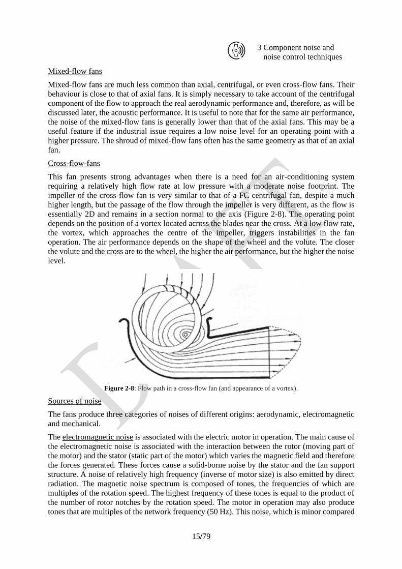
essentially 2D and remains in a section normal to the axis (Figure 2-8). The operating point

depends on the position of a vortex located across the blades near the cross. At a low flow rate,

the vortex, which approaches the centre of the impeller, triggers instabilities in the fan

operation. The air performance depends on the shape of the wheel and the volute. The closer

the volute and the cross are to the wheel, the higher the air performance, but the higher the noise

level.

Figure 2-8: Flow path in a cross-flow fan (and appearance of a vortex).

Sources of noise

The fans produce three categories of noises of different origins: aerodynamic, electromagnetic

and mechanical.

The electromagnetic noise is associated with the electric motor in operation. The main cause of

the electromagnetic noise is associated with the interaction between the rotor (moving part of

the motor) and the stator (static part of the motor) which varies the magnetic field and therefore

the forces generated. These forces cause a solid-borne noise by the stator and the fan support

structure. A noise of relatively high frequency (inverse of motor size) is also emitted by direct

radiation. The magnetic noise spectrum is composed of tones, the frequencies of which are

multiples of the rotation speed. The highest frequency of these tones is equal to the product of

the number of rotor notches by the rotation speed. The motor in operation may also produce

tones that are multiples of the network frequency (50 Hz). This noise, which is minor compared

16/79



to the aerodynamic noise and of the same order of magnitude as the mechanical noise, appears

in the spectrum of the total noise when the fan’s rotation speed is low (i.e. below about 1000

rpm).

Noticeable and annoying when the fan is kept at a low rotation speed, the mechanical noise has

its origin in vibrations induced by various phenomena:

• The occurrence of an imbalance (unbalanced wheel, alignment around an imprecise axis

of rotation...) produces vibrations at the rotation frequency.

• The bearings cause noise if they are not well maintained (bearings with worn balls or

needles or insufficiently lubricated bearings).

• The links between the motor and the fan or the support structure cause solid-borne noise

that entails radiation of the impeller and casing.

The aerodynamic noise is predominant compared to the two other sources during regular fan

operation (at or near the best efficiency point). The control of the aerodynamic noise requires

the study of the full spectrum. The noise of a fan is composed of tonal noise at the blade passing

frequency (Fpp = Nblades * Vrot) and its harmonics, and broadband noise. In their work, Lighthill,

Curle and then Ffowcs Williams-Hawkings divide the sources of aerodynamic noise into three

categories (monopolar, dipolar and quadripolar):

• For fans, the monopole noise generates a noise associated with the fluctuations of flow

due to the thickness of the blades crossing the flow. However, for the majority of fans,

the monopole noise, or thickness noise, is negligible.

• The quadrupole noise comes from the fluctuating shear stress in the turbulent flow

surrounding the blades. It becomes important for Mach number > 0.8, which never

happens on fans.

• Ultimately, only the dipolar aerodynamic noise contributes in a dominant way to the

tonal and the broadband spectrum of a fan in regular operation.

The main tonal noise generation mechanism is due to the non-uniformity of flow at the fan inlet

or outlet due to flow obstacles or non-symmetrical ducts. The variation in absolute flow velocity

at the inlet of the impeller triggers a variation of the relative speed on the blades and, therefore,

of the forces applied to them. On the other hand, for obstacles located downstream (volute cut-

off for example), a noise appears at the blade passing frequency when the wake of each blade

interacts with the volute cut-off. The experiments showed that the amplitude of the tones

increases as the upstream and downstream obstacles are closer together. Indications of the

distance between obstacles and the fan were listed in order to simplify the design of the fan

environment (for example in [47]).

The phenomena producing broadband noise are various. Fluctuations in the turbulent or laminar

flow trigger random fluctuations in the forces acting on the blades and, therefore, the impeller

radiates a broadband noise. The turbulent blade wakes also trigger the emission of broadband

noise when they meet obstacles located downstream. Other phenomena contribute to the

broadband noise:

• Noise due to ingestion of turbulence: the fluctuations of the turbulent flow velocity at

the fan inlet lead to random fluctuations in the angle of attack, resulting in random

fluctuations of the aerodynamic forces on the rotating blades and thus radiating a

broadband noise;

• Trailing edge noise: this noise occurs when the turbulent boundary layer on the blade

side (usually the suction side) is convected past the trailing edge. As a result, the

17/79



turbulent energy of the wall pressure fluctuations is converted into acoustic energy that

radiates to the far-field;

• Vortex shedding noise: this noise source, like the previous one, is located at the blade

trailing edge. It is created by the vortex shedding associated with von Karman vortex

streets in the blade wakes when the blade trailing edge is thick as compared to the

boundary layer thickness;

• Flow separation associated with rotating stall: this phenomenon may occur when the fan

is operated at a very low flow rate.

Numerical approaches

The coupling of CFD calculations and calculations of sound generation and propagation is now

offered by several computer programs or software packages. Using CFD calculations based on

Navier-Stokes equations to determine the acoustic source terms and propagation of these terms

by means of generalised Euler equations, the acoustic performance of fans starts to be predicted,

but due to the complex phenomena, a lot of research is still needed to obtain reliable results,

especially regarding the broadband noise generation.

Prediction of noise level and rules concerning similarity

Similarity

With the aim of characterising, classifying and extrapolating the noise levels measured at an

operating point, the fans required rules regarding similarity to be established. Thus, a

performance graph corresponding to one fan running at a given speed can be used to extrapolate

graphs corresponding to other speeds or fan size.

Based on measurements taken on a fan of diameter D1 and rotating at frequency V1, the air

performance of a geometrically similar fan with the characteristics {D2, V2} are determined

based on the following formulas, named “fan laws”, while limiting excessive scaling effects

(with Q volume flow rate, Δp pressure, PW fan air power and η efficiency):

Q2 = Q1 ∙V2

V1∙

D23

D13 Eq. 2

∆p2 = ∆p1 ∙V2

2

V12 ∙

D22

D12 ∙

ρ2

ρ1 Eq. 3

PW2= PW1

∙V2

3

V13 ∙

D25

D15 ∙

ρ2

ρ1 Eq. 4

η2 = η1 Eq. 5

These formulas only remain valid if the compressibility effects are negligible (Δp < 2500 Pa or

Mach < 0.3). Next, based on measurements taken on a large panel of fans, it is possible to

calculate the sound power level of fan 2 {D2, V2} from the level measured on fan 1 {D1,

V1}using the following empirical equation:

18/79



LW2= LW1

+ 10. log10

Q2

Q1+ 20. log10

∆p2

∆p1 Eq. 6

Taking into account the aerodynamic similarity rules (Eq. 2 to Eq. 5), Eq. 6 may also be written:

LW2= LW1

+ 50. log10

V2

V1+ 70. log10

D2

D1 Eq. 7

However, if the ratio of rotation speeds 𝐕𝟐/𝐕𝟏 is not close to 1, sound transposition has to be

applied not only in amplitude but also in frequency to account for the distortion of the spectrum

with speed; in fact, a high speed fan radiates emits a higher frequency noise than a low speed

fan. Therefore, AMCA (Air Movement and Control Association) proposes the following

equation for applying the conversion from conditions 1 to 2 in octave or one-third octave bands

of bandwidth BW.

LW2(f2 = f1 ∙

V2

V1) = LW1

(f1) + 40. log10

V2

V1+ 70. log10

BW2

BW1 Eq. 8

However, it should be noted that this formulation does not take into account sources whose

frequency does not depend on the rotation speed, such as an acoustic resonance resulting from

the cavity of a stator. More generally, these formulas are valid for fans without installation

effects and remain approximations.

Prediction of noise level

Given the large number of types of fans, their dimensions, their ducts upstream and

downstream, and their operating points, it appeared essential to assess the noise level of a fan

at a given operating point based on reference blowers. The sound performance of these

reference fans were obtained from comprehensive series of tests performed on a large number

of fans. These references take account of the type of fan (centrifugal or axial of different

geometry), the impeller diameter as well as the range of operating pressures. A method is

proposed by ASHRAE (American Society of Heating, Refrigerating and Air conditioning

Engineers) based on Eq. 6:

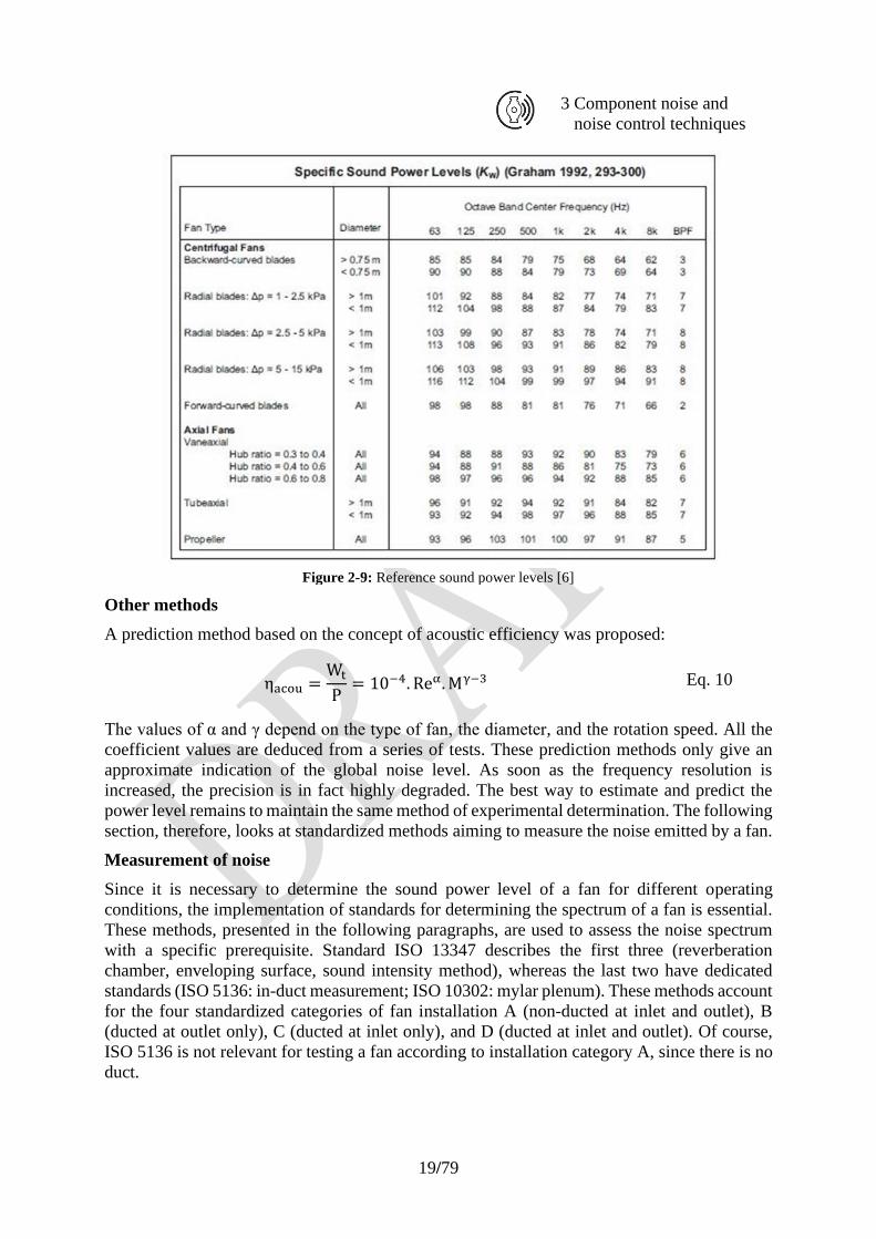
Lw(f) = Kw(f) + 10. log10

Q

Qref+ 20. log10

∆pT

∆pref Eq. 9

Where (in SI units):

• Lw(f): fan sound power level in octave band radiated by inlet + outlet + casing (dB)

• Kw(f): specific sound power level in octave band (dB) (see Table below)

• BPF: value in dB to add to Kw in the BPF octave band

• Q: fan flow rate

• ΔpT: fan total pressure

• Δpref = 1 kPa

• Qref = 1 m3/s

19/79



Figure 2-9: Reference sound power levels [6]

Other methods

A prediction method based on the concept of acoustic efficiency was proposed:

ηacou =Wt

P= 10−4. Reα. Mγ−3 Eq. 10

The values of α and γ depend on the type of fan, the diameter, and the rotation speed. All the

coefficient values are deduced from a series of tests. These prediction methods only give an

approximate indication of the global noise level. As soon as the frequency resolution is

increased, the precision is in fact highly degraded. The best way to estimate and predict the

power level remains to maintain the same method of experimental determination. The following

section, therefore, looks at standardized methods aiming to measure the noise emitted by a fan.

Measurement of noise

Since it is necessary to determine the sound power level of a fan for different operating

conditions, the implementation of standards for determining the spectrum of a fan is essential.

These methods, presented in the following paragraphs, are used to assess the noise spectrum

with a specific prerequisite. Standard ISO 13347 describes the first three (reverberation

chamber, enveloping surface, sound intensity method), whereas the last two have dedicated

standards (ISO 5136: in-duct measurement; ISO 10302: mylar plenum). These methods account

for the four standardized categories of fan installation A (non-ducted at inlet and outlet), B

(ducted at outlet only), C (ducted at inlet only), and D (ducted at inlet and outlet). Of course,

ISO 5136 is not relevant for testing a fan according to installation category A, since there is no

duct.

20/79



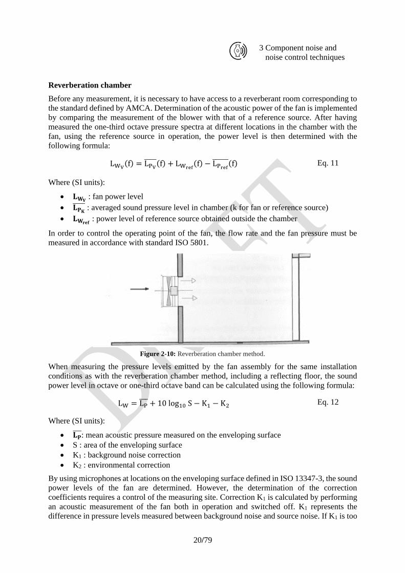
Reverberation chamber

Before any measurement, it is necessary to have access to a reverberant room corresponding to

the standard defined by AMCA. Determination of the acoustic power of the fan is implemented

by comparing the measurement of the blower with that of a reference source. After having

measured the one-third octave pressure spectra at different locations in the chamber with the

fan, using the reference source in operation, the power level is then determined with the

following formula:

LWV(f) = LPV

(f) + LWref(f) − LPref

(f) Eq. 11

Where (SI units):

• 𝐋𝐖𝐕 : fan power level

• 𝐋𝐏𝐊 : averaged sound pressure level in chamber (k for fan or reference source)

• 𝐋𝐖𝐫𝐞𝐟 : power level of reference source obtained outside the chamber

In order to control the operating point of the fan, the flow rate and the fan pressure must be

measured in accordance with standard ISO 5801.

Figure 2-10: Reverberation chamber method.

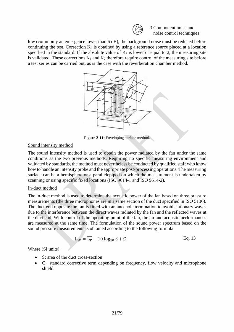
When measuring the pressure levels emitted by the fan assembly for the same installation

conditions as with the reverberation chamber method, including a reflecting floor, the sound

power level in octave or one-third octave band can be calculated using the following formula:

LW = LP + 10 log10 S − K1 − K2 Eq. 12

Where (SI units):

• 𝐋𝐏 : mean acoustic pressure measured on the enveloping surface

• S : area of the enveloping surface

• K1 : background noise correction

• K2 : environmental correction

By using microphones at locations on the enveloping surface defined in ISO 13347-3, the sound

power levels of the fan are determined. However, the determination of the correction

coefficients requires a control of the measuring site. Correction K1 is calculated by performing

an acoustic measurement of the fan both in operation and switched off. K1 represents the

difference in pressure levels measured between background noise and source noise. If K1 is too

21/79



low (commonly an emergence lower than 6 dB), the background noise must be reduced before

continuing the test. Correction K2 is obtained by using a reference source placed at a location

specified in the standard. If the absolute value of K2 is lower or equal to 2, the measuring site

is validated. These corrections K1 and K2 therefore require control of the measuring site before

a test series can be carried out, as is the case with the reverberation chamber method.

Figure 2-11: Enveloping surface method.

Sound intensity method

The sound intensity method is used to obtain the power radiated by the fan under the same

conditions as the two previous methods. Requiring no specific measuring environment and

validated by standards, the method must nevertheless be conducted by qualified staff who know

how to handle an intensity probe and the appropriate post-processing operations. The measuring

surface can be a hemisphere or a parallelepiped on which the measurement is undertaken by

scanning or using specific fixed locations (ISO 9614-1 and ISO 9614-2).

In-duct method

The in-duct method is used to determine the acoustic power of the fan based on three pressure

measurements (the three microphones are in a same section of the duct specified in ISO 5136).

The duct end opposite the fan is fitted with an anechoic termination to avoid stationary waves

due to the interference between the direct waves radiated by the fan and the reflected waves at

the duct end. With control of the operating point of the fan, the air and acoustic performances

are measured at the same time. The formulation of the sound power spectrum based on the

sound pressure measurements is obtained according to the following formula:

LW = LP + 10 log10 S + C Eq. 13

Where (SI units):

• S: area of the duct cross-section

• C : standard corrective term depending on frequency, flow velocity and microphone

shield.

22/79



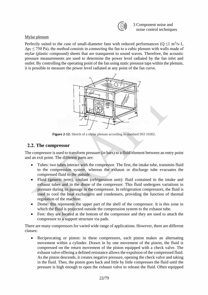
Mylar plenum

Perfectly suited to the case of small-diameter fans with reduced performances (Q ≤1 m3/s-1,

ΔpT ≤ 750 Pa), the method consists in connecting the fan to a cubic plenum with walls made of

mylar (plastic compound) sheets that are transparent to sound waves. Therefore, the acoustic

pressure measurements are used to determine the power level radiated by the fan inlet and

outlet. By controlling the operating point of the fan using static pressure taps within the plenum,

it is possible to measure the power level radiated at any point of the fan curve.

Figure 2-12: Sketch of a mylar plenum according to standard ISO 10302.

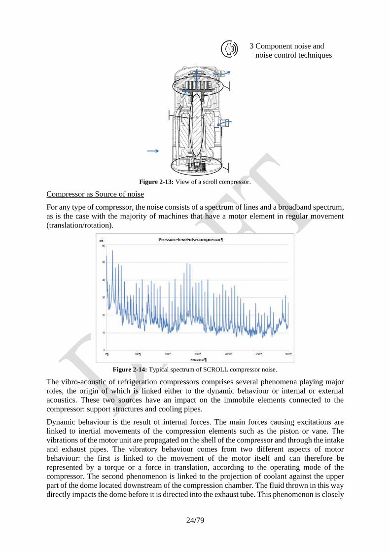
The compressor

The compressor is used to transform pressure (in bars) to a fluid element between an entry point

and an exit point. The different parts are:

• Tubes: two tubes interact with the compressor. The first, the intake tube, transmits fluid

to the compression system, whereas the exhaust or discharge tube evacuates the

compressed fluid to the outside.

• Fluid (generic term), coolant (refrigeration unit): fluid contained in the intake and

exhaust tubes and in the dome of the compressor. This fluid undergoes variations in

pressure during its passage in the compressor. In refrigeration compressors, the fluid is

used to cool the heat exchangers and condensers, providing the function of thermal

regulation of the machine.

• Dome: this represents the upper part of the shell of the compressor. It is this zone in

which the fluid is projected outside the compression system to the exhaust tube.

• Feet: they are located at the bottom of the compressor and they are used to attach the

compressor to a support structure via pads.

There are many compressors for varied wide range of applications. However, there are different

classes:

• Reciprocating or piston: in these compressors, each piston makes an alternating

movement within a cylinder. Drawn in by one movement of the piston, the fluid is

compressed on the return movement of the piston equipped with a check valve. The

exhaust valve offering a defined resistance allows the expulsion of the compressed fluid.

As the piston descends, it creates negative pressure, opening the check valve and taking

in the fluid. Then, the piston goes back and little by little compresses the fluid until the

pressure is high enough to open the exhaust valve to release the fluid. Often equipped

23/79



with several pistons with offset intake and exhaust phases, compressors ,therefore,

provide a more constant output of fluid.

• Rotary: compressor with pressure variation provided by a rotating element, as opposed

to the translational movement in piston compressors.

• Vanes: a vane compressor is composed of a cylindrical stator within which an eccentric

rotor turns. The latter is equipped with radial grooves in which vanes slide, which are

pushed against the wall of the stator by centrifugal force, so that the fluid can be sucked

in through the intake pipe and transported to the exhaust tube, the area in which the fluid

volume decreases.

• Scroll: this type of compressor requires two intercalated spirals like vanes in order to

pump and compress the fluid. One of the coils is fixed, whereas the other turns

eccentrically around the first in order to pump, hold and expel the fluid in the exhaust

tube.

• Lobe: often called a roots compressor, this is a mechanical system comprising two lobes

that hold the fluid during rotation. The compression rate is determined on the basis of

the volume held and the ratio between the speed of rotation of the lobes and that of the

motor.

• Type G: this compressor consists of two fixed spirals and two moving spirals. Driven

by the pulley of a camshaft, the mechanism is used to pump the fluid and push it towards

the centre of the compressor close to the outlet. Due to the presence of several pairs of

spirals, there is no noticeable drop in pressure between each arrival of the fluid at the

intake.

• Screw: this type of compressor consists of two counter-rotating synchronised screws

that compress the fluid. A reduction in the volume of space available for the fluid leads

to an increase pressure. The ambient fluid is drawn in along the axis of the screws, in

the area where the screw indentation is at maximum, whereas discharge is performed

after an increasingly narrow path between the screws. An oil film, cooled to increase

viscosity, ensures the compressor seal. To go through the oil film, the screws cannot get

in contact with each other and allow oil-free fluid discharge.

Several parameter influence the vibro-acoustic behaviour of compressors:

• Drive frequency: in the case of a variable speed compressor, the command frequency

corresponds to the number of iterations made by the compression element during 1

second (rps). Changing the frequency changes the motor operating speed. The

harmonics of this drive frequency will appear in the vibro-acoustic spectrum of the

compressor.

• Flow rate: linked to the compression/discharge phenomenon, the flow rate is a type of

periodic excitation (corresponding to the speed of rotation in the case of a rotary

compressor) which represents the phenomenon of expulsion of fluid towards the exhaust

tube. The value of these pressure pulsations is expressed as flow rate or as the normal

speed at the compression system outlet section.

• Torque: linked to the rotation of the motor and the friction induced, this is a secondary

contribution to the vibration and sound levels produced by the compressor.

• Pressure pulsation: the fluid ejected into the exhaust tube and circulating in the intake

tube interferes harmonically (linked to drive frequency) with the tubes that radiate and

vibrate as well as the compressor dome by repercussion.

24/79



Figure 2-13: View of a scroll compressor.

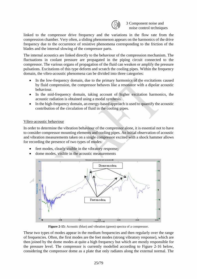
Compressor as Source of noise

For any type of compressor, the noise consists of a spectrum of lines and a broadband spectrum,

as is the case with the majority of machines that have a motor element in regular movement

(translation/rotation).

Figure 2-14: Typical spectrum of SCROLL compressor noise.

The vibro-acoustic of refrigeration compressors comprises several phenomena playing major

roles, the origin of which is linked either to the dynamic behaviour or internal or external

acoustics. These two sources have an impact on the immobile elements connected to the

compressor: support structures and cooling pipes.

Dynamic behaviour is the result of internal forces. The main forces causing excitations are

linked to inertial movements of the compression elements such as the piston or vane. The

vibrations of the motor unit are propagated on the shell of the compressor and through the intake

and exhaust pipes. The vibratory behaviour comes from two different aspects of motor

behaviour: the first is linked to the movement of the motor itself and can therefore be

represented by a torque or a force in translation, according to the operating mode of the

compressor. The second phenomenon is linked to the projection of coolant against the upper

part of the dome located downstream of the compression chamber. The fluid thrown in this way

directly impacts the dome before it is directed into the exhaust tube. This phenomenon is closely

25/79



linked to the compressor drive frequency and the variations in the flow rate from the

compression chamber. Very often, a sliding phenomenon appears on the harmonics of the drive

frequency due to the occurrence of resistive phenomena corresponding to the friction of the

blades and the internal slowing of the compressor parts.

The internal acoustics are linked directly to the behaviour of the compression mechanism. The

fluctuations in coolant pressure are propagated in the piping circuit connected to the

compressor. The various organs of propagation of the fluid can weaken or amplify the pressure

pulsations. Excitations of this type deform and scratch the cooling pipes. Within the frequency

domain, the vibro-acoustic phenomena can be divided into three categories:

• In the low-frequency domain, due to the primary harmonics of the excitations caused

by fluid compression, the compressor behaves like a resonator with a dipolar acoustic

behaviour.

• In the mid-frequency domain, taking account of higher excitation harmonics, the

acoustic radiation is obtained using a modal synthesis.

• In the high-frequency domain, an energy-based approach is used to quantify the acoustic

contribution of the circulation of fluid in the cooling pipes.

Vibro-acoustic behaviour

In order to determine the vibration behaviour of the compressor alone, it is essential not to have

to consider compressor mounting elements and cooling pipes. An initial observation of acoustic

and vibration measurements taken on a single compressor excited with a shock hammer allows

for recording the presence of two types of modes:

• feet modes, clearly visible in the vibratory response;

• dome modes, visible in the acoustic measurements

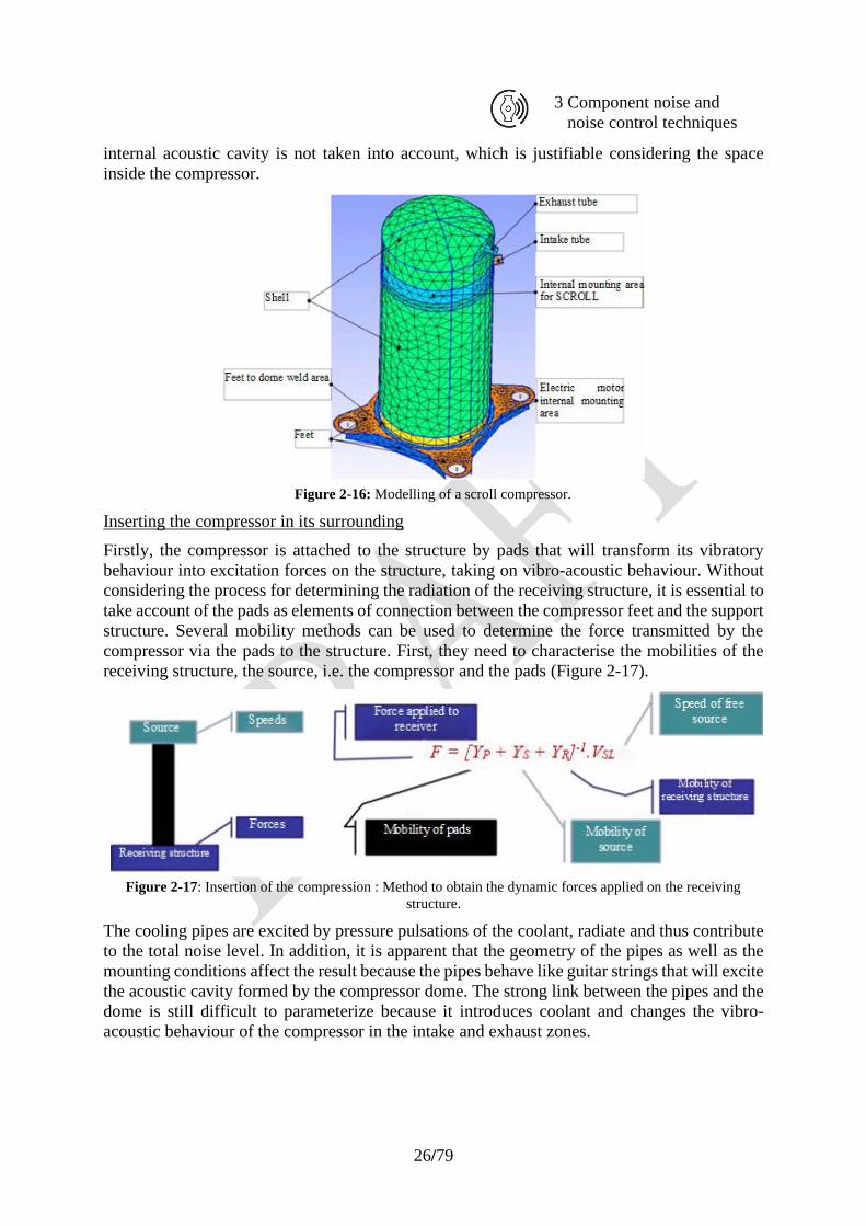
Figure 2-15: Acoustic (blue) and vibration (green) spectra of a compressor.

These two types of modes appear in the medium frequencies and then regularly over the range

of frequencies. Often, the first modes are the feet modes (strong vibratory response), which are

then joined by the dome modes at quite a high frequency but which are mostly responsible for

the pressure level. The compressor is currently modelled according to Figure 2-16 below,

considering the compressor dome as a plate that only radiates along the external normal. The

26/79



internal acoustic cavity is not taken into account, which is justifiable considering the space

inside the compressor.

Figure 2-16: Modelling of a scroll compressor.

Inserting the compressor in its surrounding

Firstly, the compressor is attached to the structure by pads that will transform its vibratory

behaviour into excitation forces on the structure, taking on vibro-acoustic behaviour. Without

considering the process for determining the radiation of the receiving structure, it is essential to

take account of the pads as elements of connection between the compressor feet and the support

structure. Several mobility methods can be used to determine the force transmitted by the

compressor via the pads to the structure. First, they need to characterise the mobilities of the

receiving structure, the source, i.e. the compressor and the pads (Figure 2-17).

Figure 2-17: Insertion of the compression : Method to obtain the dynamic forces applied on the receiving

structure.

The cooling pipes are excited by pressure pulsations of the coolant, radiate and thus contribute

to the total noise level. In addition, it is apparent that the geometry of the pipes as well as the

mounting conditions affect the result because the pipes behave like guitar strings that will excite

the acoustic cavity formed by the compressor dome. The strong link between the pipes and the

dome is still difficult to parameterize because it introduces coolant and changes the vibro-

acoustic behaviour of the compressor in the intake and exhaust zones.

27/79



Numerical prediction

The noise level calculation is carried out in three stages:

• Firstly, the excitations are calculated in relation to the characteristics of the compressor

(electrical power supply, drive frequency, dimensions, inertia, and masses of elements

in movement,...). For now, two types of excitations are considered: the flow rate of the

fluid at the compression chamber outlet and the torque applied at the inertial centre of

the element in movement (shaft for a rotation, for example).

• Next, a calculation of the vibro-acoustic response is carried out, taking account of the

two unitary excitations. This calculation is used to quantify the acoustic radiation of the

compressor dome and cooling pipes, taking the pads into account.

• To finish, the unitary response is multiplied by the excitation spectrum to obtain the

acoustic behaviour of the compressor.

As the compressor dome has a controlled vibro-acoustic behaviour, the main obstacle to this

modelling remains the quantification of the excitations and the determination of their spectra.

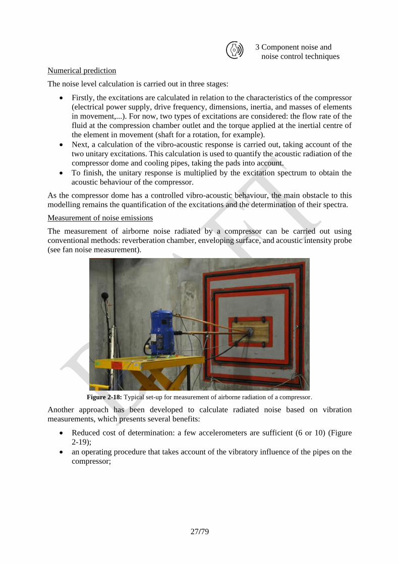
Measurement of noise emissions

The measurement of airborne noise radiated by a compressor can be carried out using

conventional methods: reverberation chamber, enveloping surface, and acoustic intensity probe

(see fan noise measurement).

Figure 2-18: Typical set-up for measurement of airborne radiation of a compressor.

Another approach has been developed to calculate radiated noise based on vibration

measurements, which presents several benefits:

• Reduced cost of determination: a few accelerometers are sufficient (6 or 10) (Figure

2-19);

• an operating procedure that takes account of the vibratory influence of the pipes on the

compressor;

28/79



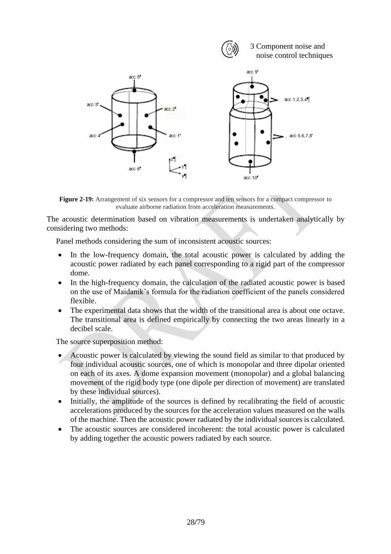
Figure 2-19: Arrangement of six sensors for a compressor and ten sensors for a compact compressor to

evaluate airborne radiation from acceleration measurements.

The acoustic determination based on vibration measurements is undertaken analytically by

considering two methods:

Panel methods considering the sum of inconsistent acoustic sources:

• In the low-frequency domain, the total acoustic power is calculated by adding the

acoustic power radiated by each panel corresponding to a rigid part of the compressor

dome.

• In the high-frequency domain, the calculation of the radiated acoustic power is based

on the use of Maidanik’s formula for the radiation coefficient of the panels considered

flexible.

• The experimental data shows that the width of the transitional area is about one octave.

The transitional area is defined empirically by connecting the two areas linearly in a

decibel scale.

The source superposition method:

• Acoustic power is calculated by viewing the sound field as similar to that produced by

four individual acoustic sources, one of which is monopolar and three dipolar oriented

on each of its axes. A dome expansion movement (monopolar) and a global balancing

movement of the rigid body type (one dipole per direction of movement) are translated

by these individual sources).

• Initially, the amplitude of the sources is defined by recalibrating the field of acoustic

accelerations produced by the sources for the acceleration values measured on the walls

of the machine. Then the acoustic power radiated by the individual sources is calculated.

• The acoustic sources are considered incoherent: the total acoustic power is calculated

by adding together the acoustic powers radiated by each source.

29/79



Secondary sources

The evaporator in an air-source heat pump is the component where heat is exchanged from the

outside air to a refrigerant in a pipe system. The most common exchanger type for modern

residential heat pumps is configured with a round tube and continuous fins. The fins are

connected to the tubing to increase the heat transfer area and can be configured as plain or wavy

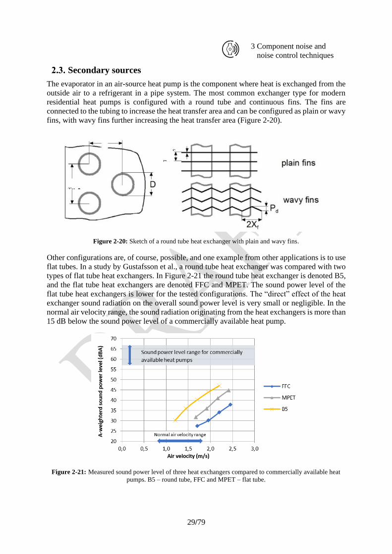
fins, with wavy fins further increasing the heat transfer area (Figure 2-20).

Figure 2-20: Sketch of a round tube heat exchanger with plain and wavy fins.

Other configurations are, of course, possible, and one example from other applications is to use

flat tubes. In a study by Gustafsson et al., a round tube heat exchanger was compared with two

types of flat tube heat exchangers. In Figure 2-21 the round tube heat exchanger is denoted B5,

and the flat tube heat exchangers are denoted FFC and MPET. The sound power level of the

flat tube heat exchangers is lower for the tested configurations. The “direct” effect of the heat

exchanger sound radiation on the overall sound power level is very small or negligible. In the

normal air velocity range, the sound radiation originating from the heat exchangers is more than

15 dB below the sound power level of a commercially available heat pump.

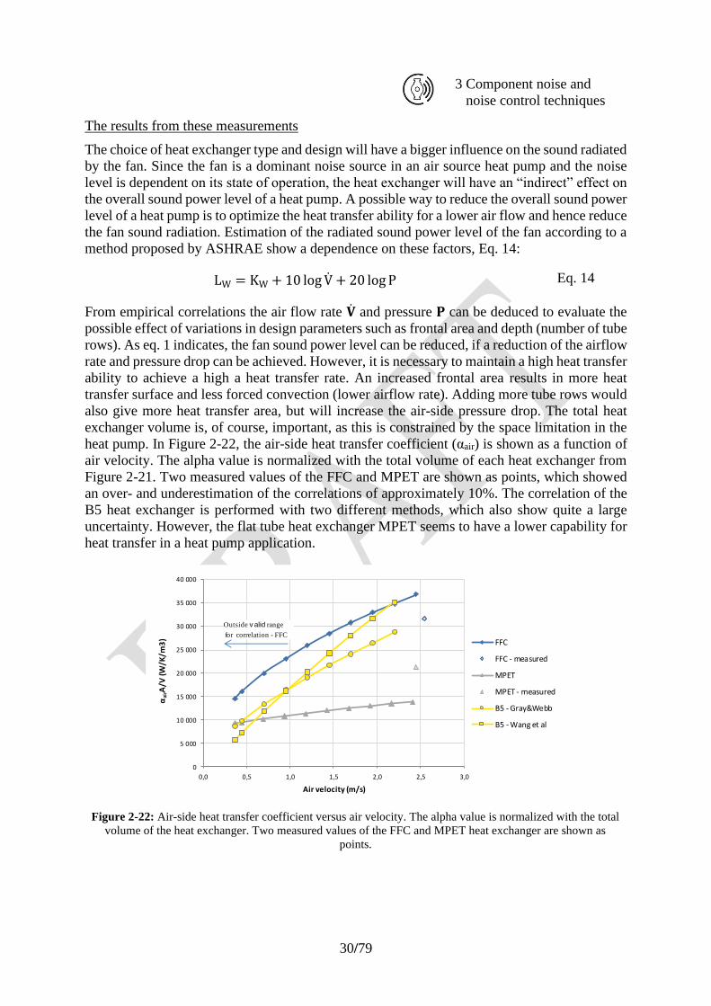
Figure 2-21: Measured sound power level of three heat exchangers compared to commercially available heat

pumps. B5 – round tube, FFC and MPET – flat tube.

30/79



The results from these measurements

The choice of heat exchanger type and design will have a bigger influence on the sound radiated

by the fan. Since the fan is a dominant noise source in an air source heat pump and the noise

level is dependent on its state of operation, the heat exchanger will have an “indirect” effect on

the overall sound power level of a heat pump. A possible way to reduce the overall sound power

level of a heat pump is to optimize the heat transfer ability for a lower air flow and hence reduce

the fan sound radiation. Estimation of the radiated sound power level of the fan according to a

method proposed by ASHRAE show a dependence on these factors, Eq. 14:

LW = KW + 10 log V + 20 log P Eq. 14

From empirical correlations the air flow rate �� and pressure 𝐏 can be deduced to evaluate the

possible effect of variations in design parameters such as frontal area and depth (number of tube

rows). As eq. 1 indicates, the fan sound power level can be reduced, if a reduction of the airflow

rate and pressure drop can be achieved. However, it is necessary to maintain a high heat transfer

ability to achieve a high a heat transfer rate. An increased frontal area results in more heat

transfer surface and less forced convection (lower airflow rate). Adding more tube rows would

also give more heat transfer area, but will increase the air-side pressure drop. The total heat

exchanger volume is, of course, important, as this is constrained by the space limitation in the

heat pump. In Figure 2-22, the air-side heat transfer coefficient (αair) is shown as a function of

air velocity. The alpha value is normalized with the total volume of each heat exchanger from

Figure 2-21. Two measured values of the FFC and MPET are shown as points, which showed

an over- and underestimation of the correlations of approximately 10%. The correlation of the

B5 heat exchanger is performed with two different methods, which also show quite a large

uncertainty. However, the flat tube heat exchanger MPET seems to have a lower capability for

heat transfer in a heat pump application.

Figure 2-22: Air-side heat transfer coefficient versus air velocity. The alpha value is normalized with the total

volume of the heat exchanger. Two measured values of the FFC and MPET heat exchanger are shown as

points.

0

5 000

10 000

15 000

20 000

25 000

30 000

35 000

40 000

0,0 0,5 1,0 1,5 2,0 2,5 3,0

αai

rA/V

(W/K

/m3

)

Air velocity (m/s)

FFC

FFC - measured

MPET

MPET - measured

B5 - Gray&Webb

B5 - Wang et al

Outside v alid range

for correlation - FFC

31/79



Heat exchangers in interaction with fan

As discussed in the previous sections, both the heat exchanger and fans contribute to the total

acoustic behaviour of a heat pump. Hence, a relevant topic for heat pump manufacturers is the

interaction between the fan and the heat exchanger and how they influence the acoustic

behaviour of each other. Several parameters, such as the distance between the components or

the angle of the heat exchanger, can have an influence on the fluid flow and, further, on the

aeroacoustic behaviour in the heat pump case. When the air enters the outdoor unit, the air

immediately flows through the heat exchanger. The fins in combination with the refrigerant

pipes or channels cause a turbulent structure in the flow field behind the heat exchanger (see

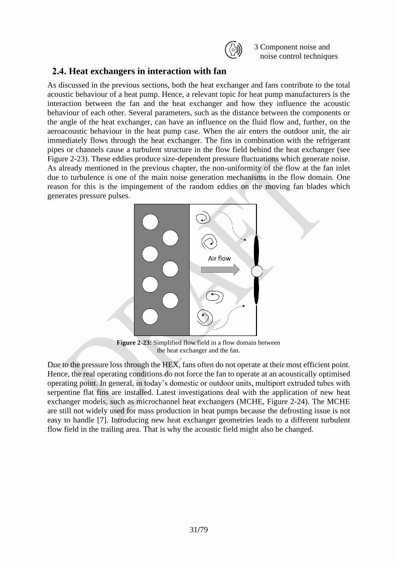
Figure 2-23). These eddies produce size-dependent pressure fluctuations which generate noise.

As already mentioned in the previous chapter, the non-uniformity of the flow at the fan inlet

due to turbulence is one of the main noise generation mechanisms in the flow domain. One

reason for this is the impingement of the random eddies on the moving fan blades which

generates pressure pulses.

Figure 2-23: Simplified flow field in a flow domain between

the heat exchanger and the fan.

Due to the pressure loss through the HEX, fans often do not operate at their most efficient point.

Hence, the real operating conditions do not force the fan to operate at an acoustically optimised

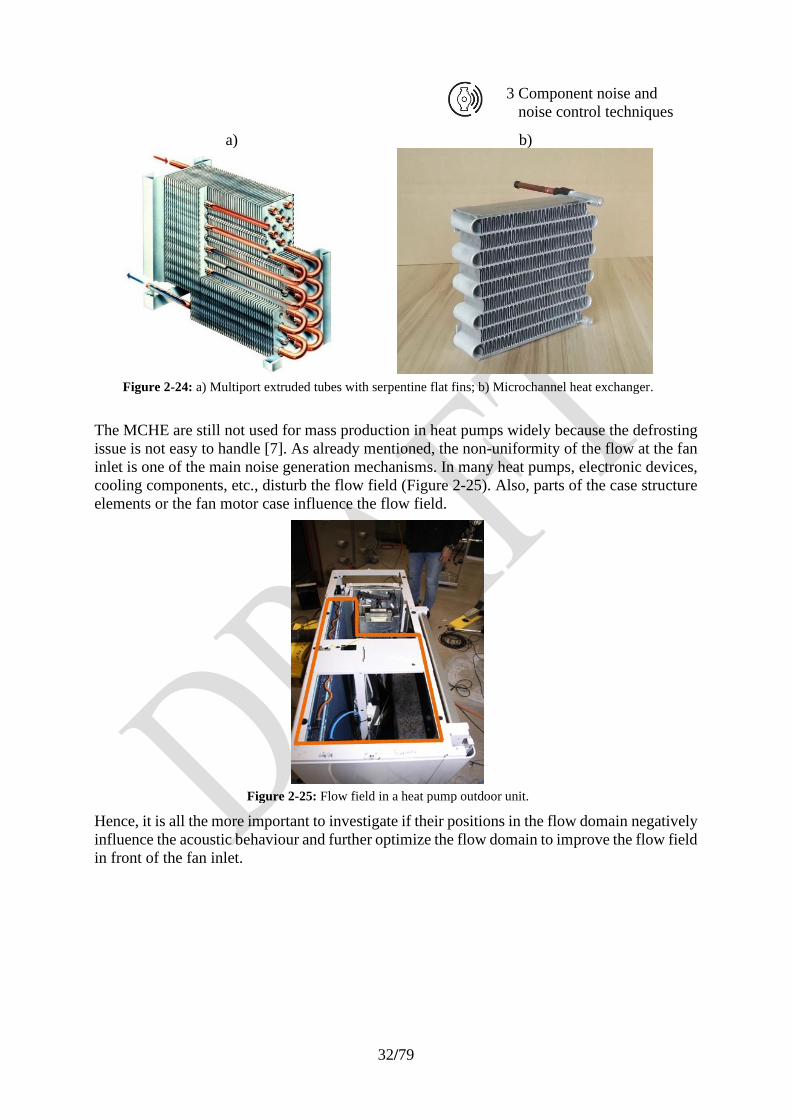
operating point. In general, in today’s domestic or outdoor units, multiport extruded tubes with

serpentine flat fins are installed. Latest investigations deal with the application of new heat

exchanger models, such as microchannel heat exchangers (MCHE, Figure 2-24). The MCHE

are still not widely used for mass production in heat pumps because the defrosting issue is not

easy to handle [7]. Introducing new heat exchanger geometries leads to a different turbulent

flow field in the trailing area. That is why the acoustic field might also be changed.

32/79



a)

b)

Figure 2-24: a) Multiport extruded tubes with serpentine flat fins; b) Microchannel heat exchanger.

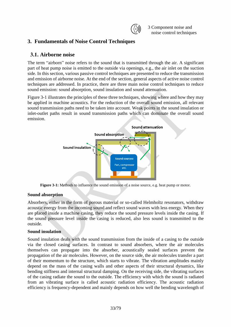
The MCHE are still not used for mass production in heat pumps widely because the defrosting

issue is not easy to handle [7]. As already mentioned, the non-uniformity of the flow at the fan

inlet is one of the main noise generation mechanisms. In many heat pumps, electronic devices,

cooling components, etc., disturb the flow field (Figure 2-25). Also, parts of the case structure

elements or the fan motor case influence the flow field.

Figure 2-25: Flow field in a heat pump outdoor unit.

Hence, it is all the more important to investigate if their positions in the flow domain negatively

influence the acoustic behaviour and further optimize the flow domain to improve the flow field

in front of the fan inlet.

33/79



3. Fundamentals of Noise Control Techniques

Airborne noise

The term “airborn” noise refers to the sound that is transmitted through the air. A significant

part of heat pump noise is emitted to the outside via openings, e.g., the air inlet on the suction

side. In this section, various passive control techniques are presented to reduce the transmission

and emission of airborne noise. At the end of the section, general aspects of active noise control

techniques are addressed. In practice, there are three main noise control techniques to reduce

sound emission: sound absorption, sound insulation and sound attenuation.

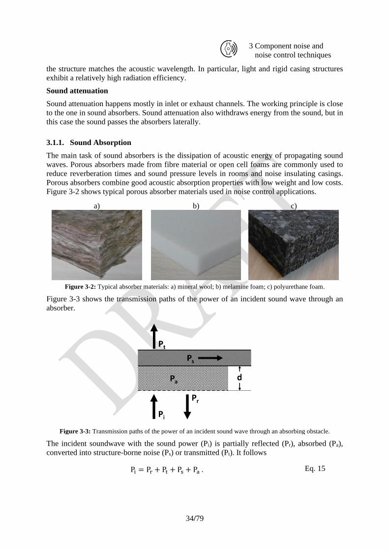
Figure 3-1 illustrates the principles of these three techniques, showing where and how they may

be applied in machine acoustics. For the reduction of the overall sound emission, all relevant

sound transmission paths need to be taken into account. Weak points in the sound insulation or

inlet-outlet paths result in sound transmission paths which can dominate the overall sound

emission.

Figure 3-1: Methods to influence the sound emission of a noise source, e.g. heat pump or motor.

Sound absorption

Absorbers, either in the form of porous material or so-called Helmholtz resonators, withdraw

acoustic energy from the incoming sound and reflect sound waves with less energy. When they

are placed inside a machine casing, they reduce the sound pressure levels inside the casing. If

the sound pressure level inside the casing is reduced, also less sound is transmitted to the

outside.

Sound insulation

Sound insulation deals with the sound transmission from the inside of a casing to the outside

via the closed casing surfaces. In contrast to sound absorbers, where the air molecules

themselves can propagate into the absorber, acoustically sealed surfaces prevent the

propagation of the air molecules. However, on the source side, the air molecules transfer a part

of their momentum to the structure, which starts to vibrate. The vibration amplitudes mainly

depend on the mass of the casing walls and other aspects of their structural dynamics, like

bending stiffness and internal structural damping. On the receiving side, the vibrating surfaces

of the casing radiate the sound to the outside. The efficiency with which the sound is radiated

from an vibrating surface is called acoustic radiation efficiency. The acoustic radiation

efficiency is frequency-dependent and mainly depends on how well the bending wavelength of

34/79



the structure matches the acoustic wavelength. In particular, light and rigid casing structures

exhibit a relatively high radiation efficiency.

Sound attenuation

Sound attenuation happens mostly in inlet or exhaust channels. The working principle is close

to the one in sound absorbers. Sound attenuation also withdraws energy from the sound, but in

this case the sound passes the absorbers laterally.

3.1.1. Sound Absorption

The main task of sound absorbers is the dissipation of acoustic energy of propagating sound

waves. Porous absorbers made from fibre material or open cell foams are commonly used to

reduce reverberation times and sound pressure levels in rooms and noise insulating casings.

Porous absorbers combine good acoustic absorption properties with low weight and low costs.

Figure 3-2 shows typical porous absorber materials used in noise control applications.

Figure 3-3 shows the transmission paths of the power of an incident sound wave through an

absorber.

Figure 3-3: Transmission paths of the power of an incident sound wave through an absorbing obstacle.

The incident soundwave with the sound power (Pi) is partially reflected (Pr), absorbed (Pa),

converted into structure-borne noise (Ps) or transmitted (Pt). It follows

Pi = Pr + Pt + Ps + Pa . Eq. 15

a) b) c)

Figure 3-2: Typical absorber materials: a) mineral wool; b) melamine foam; c) polyurethane foam.

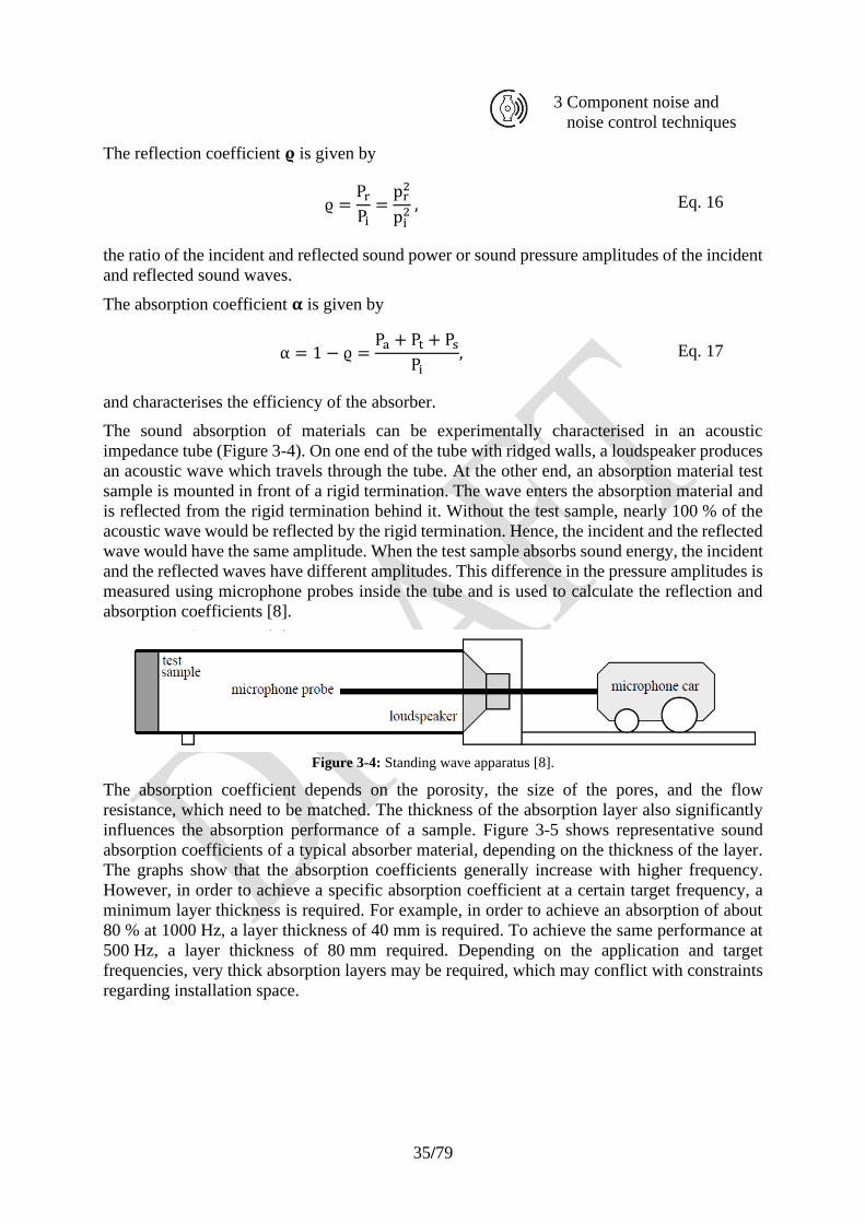
35/79



The reflection coefficient 𝛠 is given by

ϱ =Pr

Pi=

pr2

pi2 , Eq. 16

the ratio of the incident and reflected sound power or sound pressure amplitudes of the incident

and reflected sound waves.

The absorption coefficient 𝛂 is given by

α = 1 − ϱ =Pa + Pt + Ps

Pi, Eq. 17

and characterises the efficiency of the absorber.

The sound absorption of materials can be experimentally characterised in an acoustic

impedance tube (Figure 3-4). On one end of the tube with ridged walls, a loudspeaker produces

an acoustic wave which travels through the tube. At the other end, an absorption material test

sample is mounted in front of a rigid termination. The wave enters the absorption material and

is reflected from the rigid termination behind it. Without the test sample, nearly 100 % of the

acoustic wave would be reflected by the rigid termination. Hence, the incident and the reflected

wave would have the same amplitude. When the test sample absorbs sound energy, the incident

and the reflected waves have different amplitudes. This difference in the pressure amplitudes is

measured using microphone probes inside the tube and is used to calculate the reflection and

absorption coefficients [8].

Figure 3-4: Standing wave apparatus [8].

The absorption coefficient depends on the porosity, the size of the pores, and the flow

resistance, which need to be matched. The thickness of the absorption layer also significantly

influences the absorption performance of a sample. Figure 3-5 shows representative sound

absorption coefficients of a typical absorber material, depending on the thickness of the layer.

The graphs show that the absorption coefficients generally increase with higher frequency.

However, in order to achieve a specific absorption coefficient at a certain target frequency, a

minimum layer thickness is required. For example, in order to achieve an absorption of about

80 % at 1000 Hz, a layer thickness of 40 mm is required. To achieve the same performance at

500 Hz, a layer thickness of 80 mm required. Depending on the application and target

frequencies, very thick absorption layers may be required, which may conflict with constraints

regarding installation space.

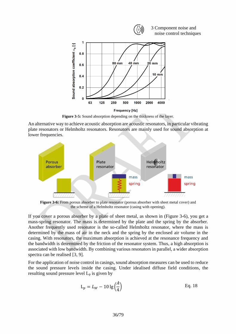
36/79



Figure 3-5: Sound absorption depending on the thickness of the layer.

An alternative way to achieve acoustic absorption are acoustic resonators, in particular vibrating

plate resonators or Helmholtz resonators. Resonators are mainly used for sound absorption at

lower frequencies.

Figure 3-6: From porous absorber to plate resonator (porous absorber with sheet metal cover) and

the scheme of a Helmholtz resonator (casing with opening).

If you cover a porous absorber by a plate of sheet metal, as shown in (Figure 3-6), you get a

mass-spring resonator. The mass is determined by the plate and the spring by the absorber.

Another frequently used resonator is the so-called Helmholtz resonator, where the mass is

determined by the mass of air in the neck and the spring by the enclosed air volume in the

casing. With resonators, the maximum absorption is achieved at the resonance frequency and

the bandwidth is determined by the friction of the resonator system. Thus, a high absorption is

associated with low bandwidth. By combining various resonators in parallel, a wider absorption

spectra can be realised [3, 9].

For the application of noise control in casings, sound absorption measures can be used to reduce

the sound pressure levels inside the casing. Under idealised diffuse field conditions, the

resulting sound pressure level Lp is given by

L𝑝 = 𝐿𝑊 − 10 lg (𝐴

4) Eq. 18

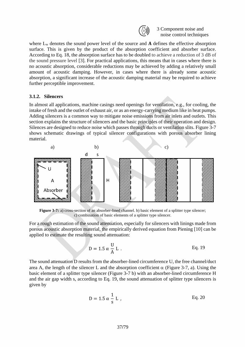
37/79



where Lw denotes the sound power level of the source and 𝐀 defines the effective absorption

surface. This is given by the product of the absorption coefficient and absorber surface.

According to Eq. 18, the absorption surface has to be doubled to achieve a reduction of 3 dB of

the sound pressure level [3]. For practical applications, this means that in cases where there is

no acoustic absorption, considerable reductions may be achieved by adding a relatively small

amount of acoustic damping. However, in cases where there is already some acoustic

absorption, a significant increase of the acoustic damping material may be required to achieve

further perceptible improvement.

3.1.2. Silencers

In almost all applications, machine casings need openings for ventilation, e.g., for cooling, the

intake of fresh and the outlet of exhaust air, or as an energy-carrying medium like in heat pumps.

Adding silencers is a common way to mitigate noise emissions from air inlets and outlets. This

section explains the structure of silencers and the basic principles of their operation and design.

Silences are designed to reduce noise which passes through ducts or ventilation slits. Figure 3-7

shows schematic drawings of typical silencer configurations with porous absorber lining

material.

a) b) c)

Figure 3-7: a) cross-section of an absorber-lined channel. b) basic element of a splitter type silencer;

c) combination of basic elements of a splitter type silencer.

For a rough estimation of the sound attenuation, especially for silencers with linings made from

porous acoustic absorption material, the empirically derived equation from Piening [10] can be

applied to estimate the resulting sound attenuation:

D = 1.5 α U

A L . Eq. 19

The sound attenuation D results from the absorber-lined circumference U, the free channel/duct

area A, the length of the silencer L and the absorption coefficient (Figure 3-7, a). Using the

basic element of a splitter type silencer (Figure 3-7 b) with an absorber-lined circumference H

and the air gap width s, according to Eq. 19, the sound attenuation of splitter type silencers is

given by

D = 1.5 α 1

s L , Eq. 20

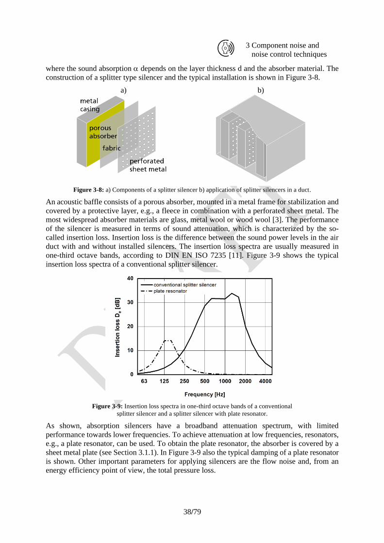
38/79



where the sound absorption depends on the layer thickness d and the absorber material. The

construction of a splitter type silencer and the typical installation is shown in Figure 3-8.

a) b)

Figure 3-8: a) Components of a splitter silencer b) application of splitter silencers in a duct.

An acoustic baffle consists of a porous absorber, mounted in a metal frame for stabilization and

covered by a protective layer, e.g., a fleece in combination with a perforated sheet metal. The

most widespread absorber materials are glass, metal wool or wood wool [3]. The performance

of the silencer is measured in terms of sound attenuation, which is characterized by the so-

called insertion loss. Insertion loss is the difference between the sound power levels in the air

duct with and without installed silencers. The insertion loss spectra are usually measured in

one-third octave bands, according to DIN EN ISO 7235 [11]. Figure 3-9 shows the typical

insertion loss spectra of a conventional splitter silencer.

Figure 3-9: Insertion loss spectra in one-third octave bands of a conventional

splitter silencer and a splitter silencer with plate resonator.

As shown, absorption silencers have a broadband attenuation spectrum, with limited

performance towards lower frequencies. To achieve attenuation at low frequencies, resonators,

e.g., a plate resonator, can be used. To obtain the plate resonator, the absorber is covered by a

sheet metal plate (see Section 3.1.1). In Figure 3-9 also the typical damping of a plate resonator

is shown. Other important parameters for applying silencers are the flow noise and, from an

energy efficiency point of view, the total pressure loss.

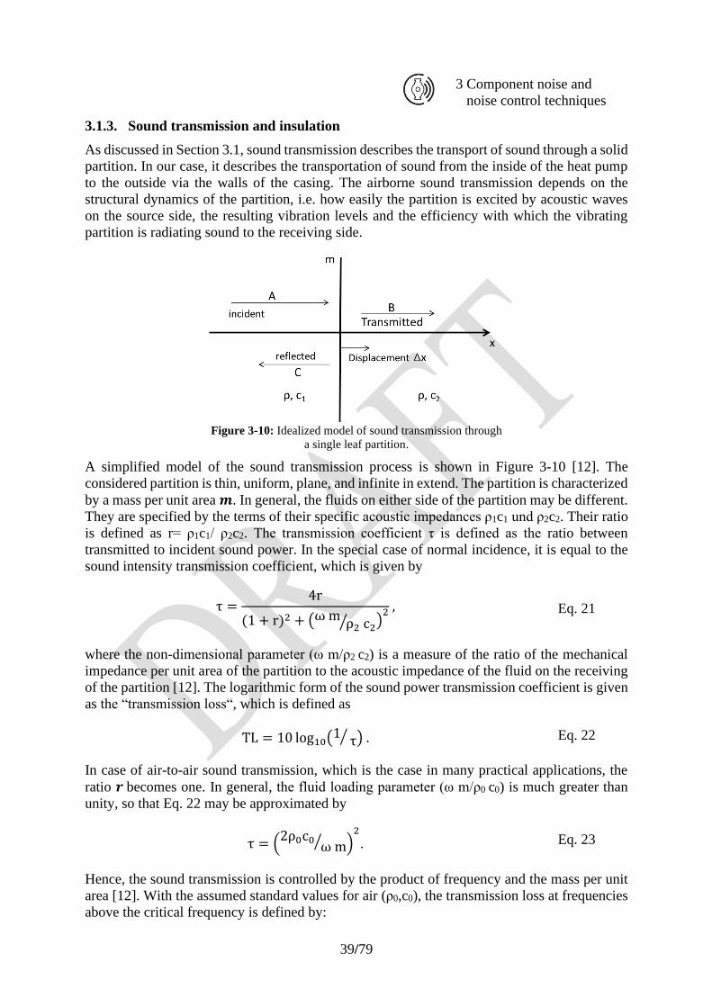
39/79



3.1.3. Sound transmission and insulation

As discussed in Section 3.1, sound transmission describes the transport of sound through a solid

partition. In our case, it describes the transportation of sound from the inside of the heat pump

to the outside via the walls of the casing. The airborne sound transmission depends on the

structural dynamics of the partition, i.e. how easily the partition is excited by acoustic waves

on the source side, the resulting vibration levels and the efficiency with which the vibrating

partition is radiating sound to the receiving side.

Figure 3-10: Idealized model of sound transmission through

a single leaf partition.

A simplified model of the sound transmission process is shown in Figure 3-10 [12]. The

considered partition is thin, uniform, plane, and infinite in extend. The partition is characterized

by a mass per unit area 𝒎. In general, the fluids on either side of the partition may be different.

They are specified by the terms of their specific acoustic impedances ρ1c1 und ρ2c2. Their ratio

is defined as r= ρ1c1/ ρ2c2. The transmission coefficient τ is defined as the ratio between

transmitted to incident sound power. In the special case of normal incidence, it is equal to the

sound intensity transmission coefficient, which is given by

τ =4r

(1 + r)2 + (ω mρ2 c2⁄ )

2 , Eq. 21

where the non-dimensional parameter (ω m/ρ2 c2) is a measure of the ratio of the mechanical

impedance per unit area of the partition to the acoustic impedance of the fluid on the receiving

of the partition [12]. The logarithmic form of the sound power transmission coefficient is given

as the “transmission loss“, which is defined as

TL = 10 log10(1 τ⁄ ) . Eq. 22

In case of air-to-air sound transmission, which is the case in many practical applications, the

ratio 𝒓 becomes one. In general, the fluid loading parameter (ω m/ρ0 c0) is much greater than

unity, so that Eq. 22 may be approximated by

τ = (2ρ0c0

ω m⁄ )2

. Eq. 23

Hence, the sound transmission is controlled by the product of frequency and the mass per unit

area [12]. With the assumed standard values for air (ρ0,c0), the transmission loss at frequencies

above the critical frequency is defined by:

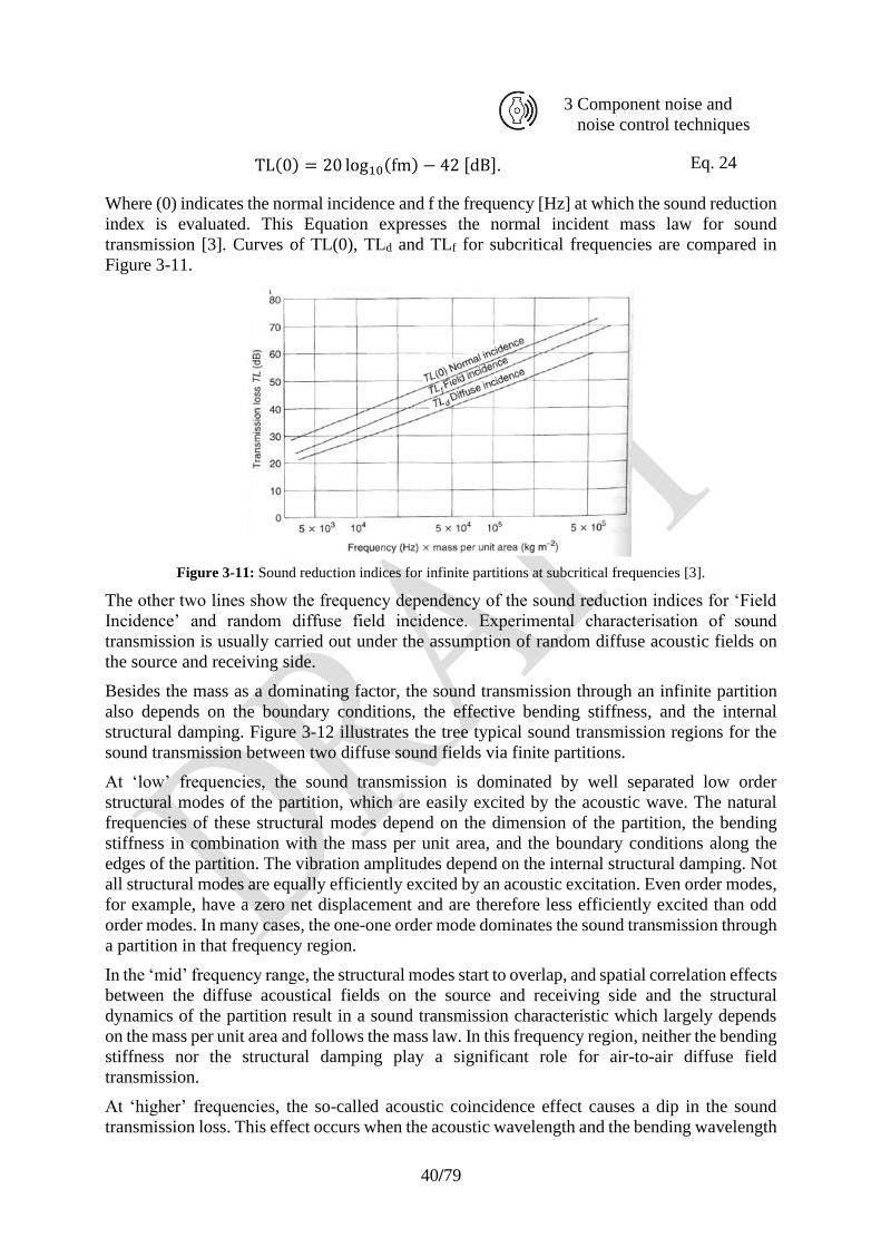
40/79



TL(0) = 20 log10(fm) − 42 [dB]. Eq. 24

Where (0) indicates the normal incidence and f the frequency [Hz] at which the sound reduction

index is evaluated. This Equation expresses the normal incident mass law for sound

transmission [3]. Curves of TL(0), TLd and TLf for subcritical frequencies are compared in

Figure 3-11.

Figure 3-11: Sound reduction indices for infinite partitions at subcritical frequencies [3].

The other two lines show the frequency dependency of the sound reduction indices for ‘Field

Incidence’ and random diffuse field incidence. Experimental characterisation of sound

transmission is usually carried out under the assumption of random diffuse acoustic fields on

the source and receiving side.

Besides the mass as a dominating factor, the sound transmission through an infinite partition

also depends on the boundary conditions, the effective bending stiffness, and the internal

structural damping. Figure 3-12 illustrates the tree typical sound transmission regions for the

sound transmission between two diffuse sound fields via finite partitions.

At ‘low’ frequencies, the sound transmission is dominated by well separated low order

structural modes of the partition, which are easily excited by the acoustic wave. The natural

frequencies of these structural modes depend on the dimension of the partition, the bending

stiffness in combination with the mass per unit area, and the boundary conditions along the

edges of the partition. The vibration amplitudes depend on the internal structural damping. Not

all structural modes are equally efficiently excited by an acoustic excitation. Even order modes,

for example, have a zero net displacement and are therefore less efficiently excited than odd

order modes. In many cases, the one-one order mode dominates the sound transmission through

a partition in that frequency region.

In the ‘mid’ frequency range, the structural modes start to overlap, and spatial correlation effects

between the diffuse acoustical fields on the source and receiving side and the structural

dynamics of the partition result in a sound transmission characteristic which largely depends

on the mass per unit area and follows the mass law. In this frequency region, neither the bending

stiffness nor the structural damping play a significant role for air-to-air diffuse field

transmission.

At ‘higher’ frequencies, the so-called acoustic coincidence effect causes a dip in the sound

transmission loss. This effect occurs when the acoustic wavelength and the bending wavelength

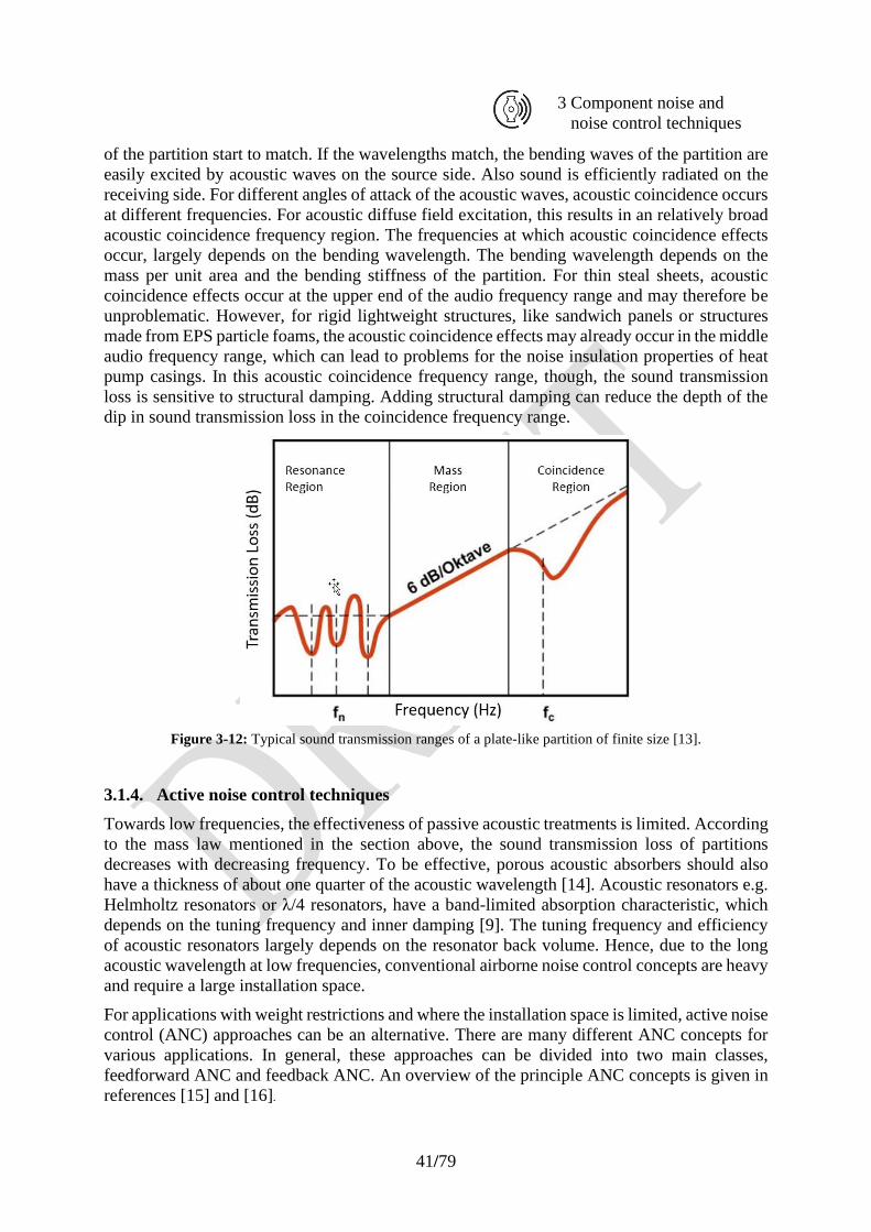
41/79



of the partition start to match. If the wavelengths match, the bending waves of the partition are

easily excited by acoustic waves on the source side. Also sound is efficiently radiated on the

receiving side. For different angles of attack of the acoustic waves, acoustic coincidence occurs

at different frequencies. For acoustic diffuse field excitation, this results in an relatively broad

acoustic coincidence frequency region. The frequencies at which acoustic coincidence effects

occur, largely depends on the bending wavelength. The bending wavelength depends on the

mass per unit area and the bending stiffness of the partition. For thin steal sheets, acoustic

coincidence effects occur at the upper end of the audio frequency range and may therefore be

unproblematic. However, for rigid lightweight structures, like sandwich panels or structures

made from EPS particle foams, the acoustic coincidence effects may already occur in the middle

audio frequency range, which can lead to problems for the noise insulation properties of heat

pump casings. In this acoustic coincidence frequency range, though, the sound transmission

loss is sensitive to structural damping. Adding structural damping can reduce the depth of the

dip in sound transmission loss in the coincidence frequency range.

Figure 3-12: Typical sound transmission ranges of a plate-like partition of finite size [13].

3.1.4. Active noise control techniques

Towards low frequencies, the effectiveness of passive acoustic treatments is limited. According

to the mass law mentioned in the section above, the sound transmission loss of partitions

decreases with decreasing frequency. To be effective, porous acoustic absorbers should also

have a thickness of about one quarter of the acoustic wavelength [14]. Acoustic resonators e.g.

Helmholtz resonators or λ/4 resonators, have a band-limited absorption characteristic, which

depends on the tuning frequency and inner damping [9]. The tuning frequency and efficiency

of acoustic resonators largely depends on the resonator back volume. Hence, due to the long

acoustic wavelength at low frequencies, conventional airborne noise control concepts are heavy

and require a large installation space.

For applications with weight restrictions and where the installation space is limited, active noise

control (ANC) approaches can be an alternative. There are many different ANC concepts for

various applications. In general, these approaches can be divided into two main classes,

feedforward ANC and feedback ANC. An overview of the principle ANC concepts is given in

references [15] and [16].

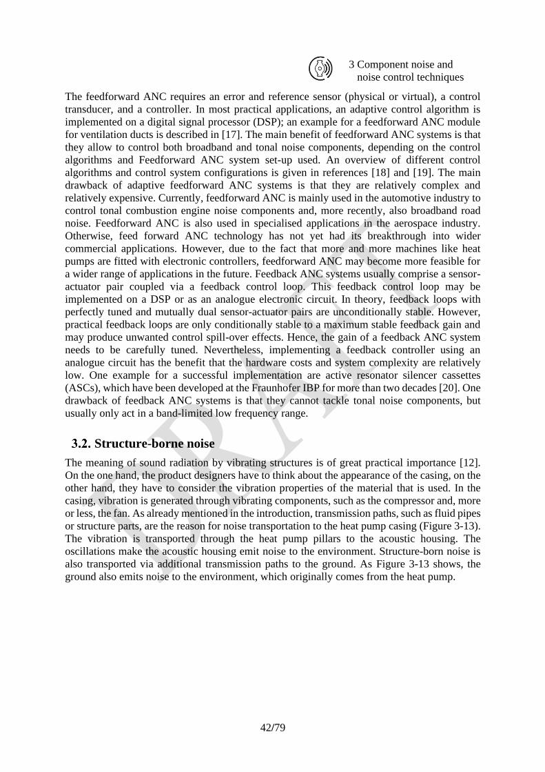
42/79



The feedforward ANC requires an error and reference sensor (physical or virtual), a control

transducer, and a controller. In most practical applications, an adaptive control algorithm is

implemented on a digital signal processor (DSP); an example for a feedforward ANC module

for ventilation ducts is described in [17]. The main benefit of feedforward ANC systems is that

they allow to control both broadband and tonal noise components, depending on the control

algorithms and Feedforward ANC system set-up used. An overview of different control

algorithms and control system configurations is given in references [18] and [19]. The main

drawback of adaptive feedforward ANC systems is that they are relatively complex and

relatively expensive. Currently, feedforward ANC is mainly used in the automotive industry to

control tonal combustion engine noise components and, more recently, also broadband road

noise. Feedforward ANC is also used in specialised applications in the aerospace industry.

Otherwise, feed forward ANC technology has not yet had its breakthrough into wider

commercial applications. However, due to the fact that more and more machines like heat

pumps are fitted with electronic controllers, feedforward ANC may become more feasible for

a wider range of applications in the future. Feedback ANC systems usually comprise a sensor-

actuator pair coupled via a feedback control loop. This feedback control loop may be

implemented on a DSP or as an analogue electronic circuit. In theory, feedback loops with

perfectly tuned and mutually dual sensor-actuator pairs are unconditionally stable. However,

practical feedback loops are only conditionally stable to a maximum stable feedback gain and

may produce unwanted control spill-over effects. Hence, the gain of a feedback ANC system

needs to be carefully tuned. Nevertheless, implementing a feedback controller using an

analogue circuit has the benefit that the hardware costs and system complexity are relatively

low. One example for a successful implementation are active resonator silencer cassettes

(ASCs), which have been developed at the Fraunhofer IBP for more than two decades [20]. One

drawback of feedback ANC systems is that they cannot tackle tonal noise components, but

usually only act in a band-limited low frequency range.

Structure-borne noise

The meaning of sound radiation by vibrating structures is of great practical importance [12].

On the one hand, the product designers have to think about the appearance of the casing, on the

other hand, they have to consider the vibration properties of the material that is used. In the

casing, vibration is generated through vibrating components, such as the compressor and, more

or less, the fan. As already mentioned in the introduction, transmission paths, such as fluid pipes

or structure parts, are the reason for noise transportation to the heat pump casing (Figure 3-13).

The vibration is transported through the heat pump pillars to the acoustic housing. The

oscillations make the acoustic housing emit noise to the environment. Structure-born noise is

also transported via additional transmission paths to the ground. As Figure 3-13 shows, the

ground also emits noise to the environment, which originally comes from the heat pump.

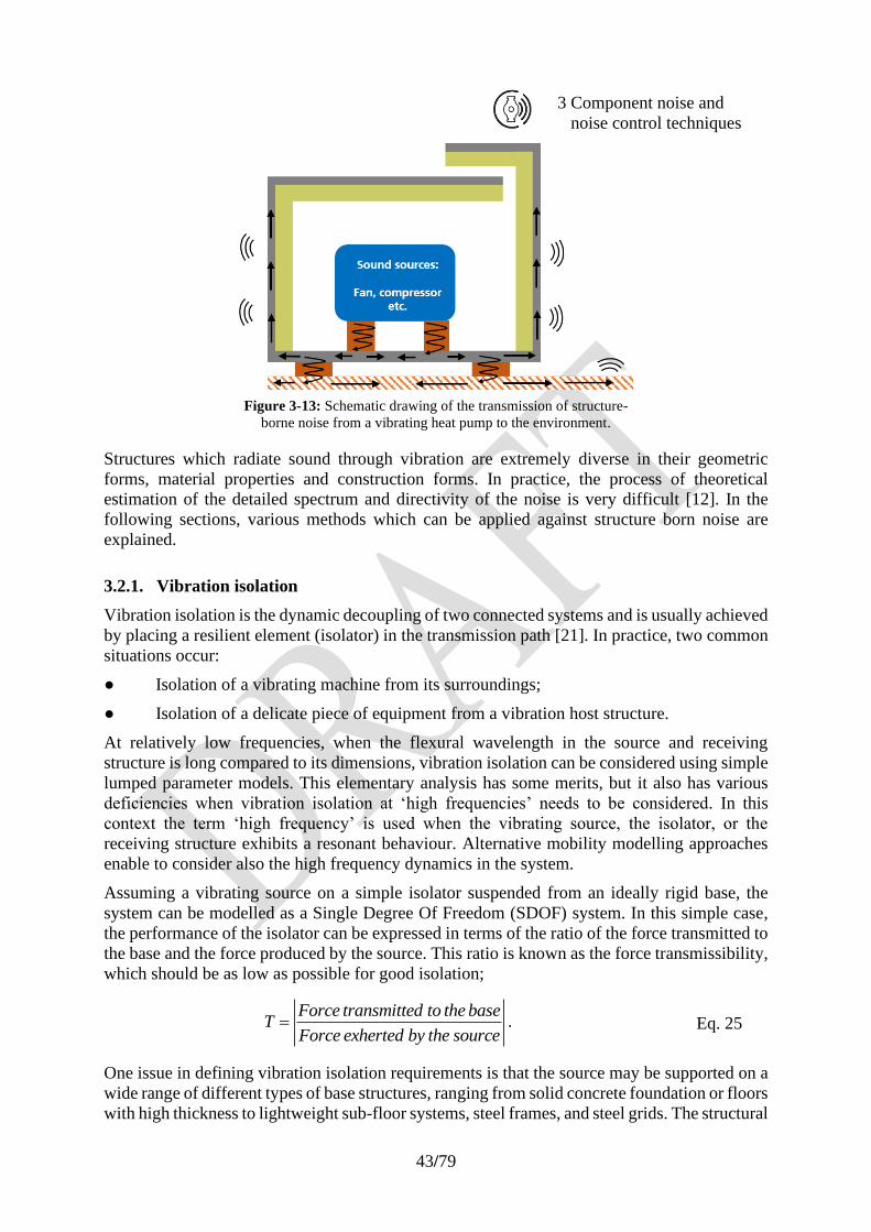
43/79



Figure 3-13: Schematic drawing of the transmission of structure-

borne noise from a vibrating heat pump to the environment.

Structures which radiate sound through vibration are extremely diverse in their geometric

forms, material properties and construction forms. In practice, the process of theoretical

estimation of the detailed spectrum and directivity of the noise is very difficult [12]. In the

following sections, various methods which can be applied against structure born noise are

explained.

3.2.1. Vibration isolation

Vibration isolation is the dynamic decoupling of two connected systems and is usually achieved

by placing a resilient element (isolator) in the transmission path [21]. In practice, two common

situations occur:

● Isolation of a vibrating machine from its surroundings;

● Isolation of a delicate piece of equipment from a vibration host structure.

At relatively low frequencies, when the flexural wavelength in the source and receiving

structure is long compared to its dimensions, vibration isolation can be considered using simple

lumped parameter models. This elementary analysis has some merits, but it also has various

deficiencies when vibration isolation at ‘high frequencies’ needs to be considered. In this

context the term ‘high frequency’ is used when the vibrating source, the isolator, or the

receiving structure exhibits a resonant behaviour. Alternative mobility modelling approaches

enable to consider also the high frequency dynamics in the system.

Assuming a vibrating source on a simple isolator suspended from an ideally rigid base, the

system can be modelled as a Single Degree Of Freedom (SDOF) system. In this simple case,

the performance of the isolator can be expressed in terms of the ratio of the force transmitted to

the base and the force produced by the source. This ratio is known as the force transmissibility,

which should be as low as possible for good isolation;

Force transmitted to the baseT

Force exherted by the source

=

. Eq. 25

One issue in defining vibration isolation requirements is that the source may be supported on a

wide range of different types of base structures, ranging from solid concrete foundation or floors

with high thickness to lightweight sub-floor systems, steel frames, and steel grids. The structural

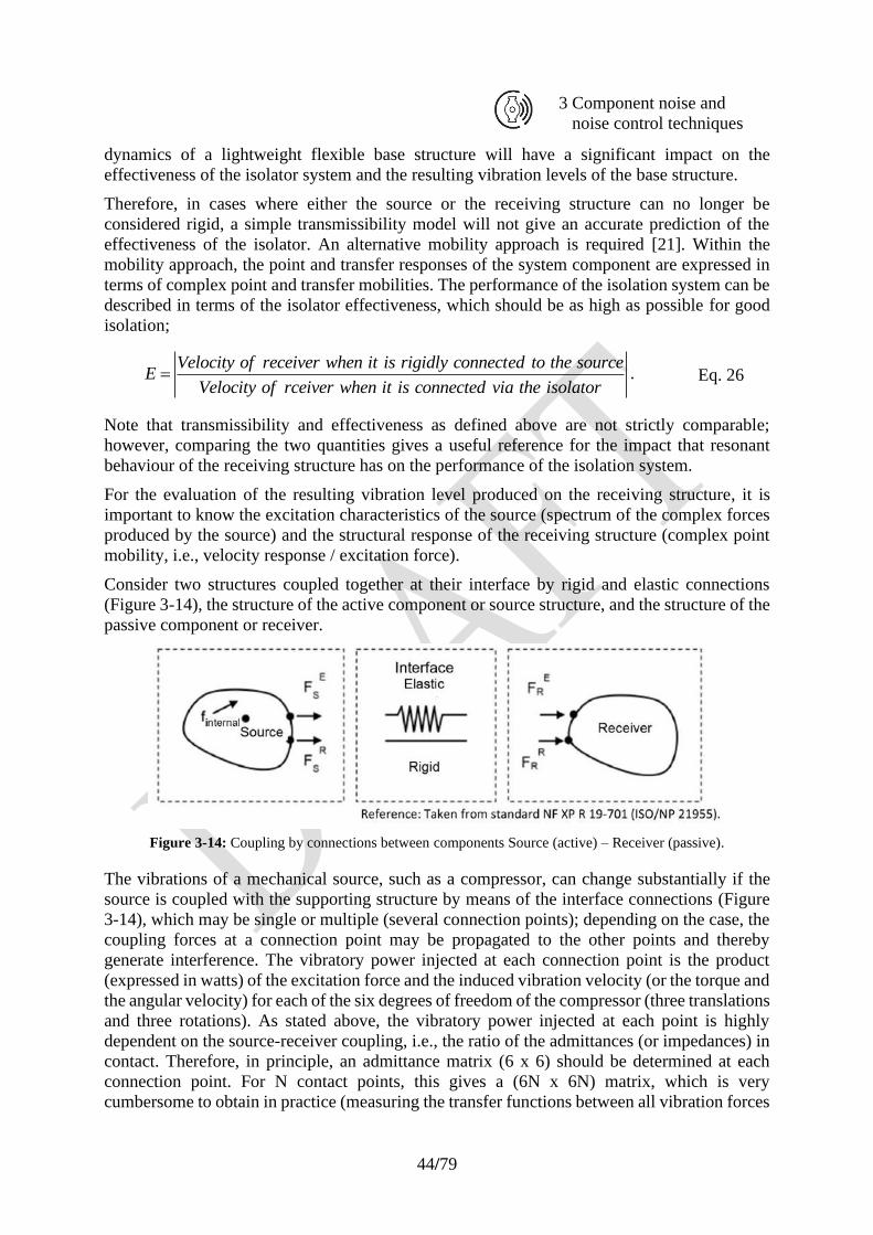
44/79



dynamics of a lightweight flexible base structure will have a significant impact on the

effectiveness of the isolator system and the resulting vibration levels of the base structure.

Therefore, in cases where either the source or the receiving structure can no longer be

considered rigid, a simple transmissibility model will not give an accurate prediction of the

effectiveness of the isolator. An alternative mobility approach is required [21]. Within the

mobility approach, the point and transfer responses of the system component are expressed in

terms of complex point and transfer mobilities. The performance of the isolation system can be

described in terms of the isolator effectiveness, which should be as high as possible for good

isolation;

Velocity of receiver when it is rigidly connected to the sourceE

Velocity of rceiver when it is connected via the isolator= . Eq. 26

Note that transmissibility and effectiveness as defined above are not strictly comparable;

however, comparing the two quantities gives a useful reference for the impact that resonant

behaviour of the receiving structure has on the performance of the isolation system.

For the evaluation of the resulting vibration level produced on the receiving structure, it is

important to know the excitation characteristics of the source (spectrum of the complex forces

produced by the source) and the structural response of the receiving structure (complex point

mobility, i.e., velocity response / excitation force).

Consider two structures coupled together at their interface by rigid and elastic connections

(Figure 3-14), the structure of the active component or source structure, and the structure of the

passive component or receiver.

Figure 3-14: Coupling by connections between components Source (active) – Receiver (passive).

The vibrations of a mechanical source, such as a compressor, can change substantially if the

source is coupled with the supporting structure by means of the interface connections (Figure

3-14), which may be single or multiple (several connection points); depending on the case, the

coupling forces at a connection point may be propagated to the other points and thereby

generate interference. The vibratory power injected at each connection point is the product

(expressed in watts) of the excitation force and the induced vibration velocity (or the torque and

the angular velocity) for each of the six degrees of freedom of the compressor (three translations

and three rotations). As stated above, the vibratory power injected at each point is highly

dependent on the source-receiver coupling, i.e., the ratio of the admittances (or impedances) in

contact. Therefore, in principle, an admittance matrix (6 x 6) should be determined at each

connection point. For N contact points, this gives a (6N x 6N) matrix, which is very

cumbersome to obtain in practice (measuring the transfer functions between all vibration forces

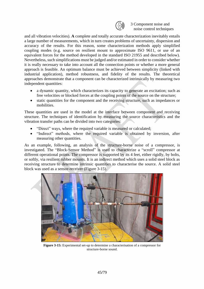
45/79



and all vibration velocities). A complete and totally accurate characterization inevitably entails

a large number of measurements, which in turn creates problems of uncertainty, dispersion and

accuracy of the results. For this reason, some characterization methods apply simplified

coupling modes (e.g. source on resilient mount to approximate ISO 9611, or use of an

equivalent forces for the method developed in the standard ISO 21955 and described below).

Nevertheless, such simplifications must be judged and/or estimated in order to consider whether

it is really necessary to take into account all the connection points or whether a more general

approach is feasible. An optimum balance must be achieved between simplicity (linked with

industrial application), method robustness, and fidelity of the results. The theoretical

approaches demonstrate that a component can be characterized intrinsically by measuring two

independent quantities:

• a dynamic quantity, which characterizes its capacity to generate an excitation; such as

free velocities or blocked forces at the coupling points of the source on the structure;

• static quantities for the component and the receiving structure, such as impedances or

mobilities.

These quantities are used in the model at the interface between component and receiving

structure. The techniques of identification by measuring the source characteristics and the

vibration transfer paths can be divided into two categories:

• “Direct” ways, where the required variable is measured or calculated;

• “Indirect” methods, where the required variable is obtained by inversion, after

measuring other quantities.

As an example, following, an analysis of the structure-borne noise of a compressor, is

investigated. The “Block-Sensor Method” is used to characterize a “scroll” compressor at

different operational points. The compressor is supported by its 4 feet, either rigidly, by bolts,

or softly, via resilient rubber mounts. It is an indirect method which uses a solid steel block as

receiving structure to determine intrinsic quantities to characterise the source. A solid steel

block was used as a sensor-receiver (Figure 3-15).

Figure 3-15: Experimental set-up to determine a characterisation of a compressor for

structure-borne sound.

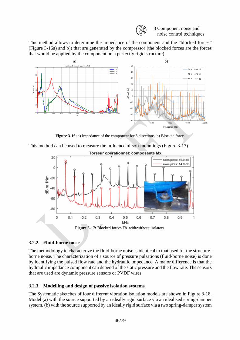
46/79



This method allows to determine the impedance of the component and the “blocked forces”

(Figure 3-16a) and b)) that are generated by the compressor (the blocked forces are the forces

that would be applied by the component on a perfectly rigid structure).

a) b)

Figure 3-16: a) Impedance of the component for 3 directions; b) Blocked force.

This method can be used to measure the influence of soft mountings (Figure 3-17).

Figure 3-17: Blocked forces Fb with/without isolators.

3.2.2. Fluid-borne noise

The methodology to characterize the fluid-borne noise is identical to that used for the structure-

borne noise. The characterization of a source of pressure pulsations (fluid-borne noise) is done

by identifying the pulsed flow rate and the hydraulic impedance. A major difference is that the

hydraulic impedance component can depend of the static pressure and the flow rate. The sensors

that are used are dynamic pressure sensors or PVDF wires.

3.2.3. Modelling and design of passive isolation systems

The Systematic sketches of four different vibration isolation models are shown in Figure 3-18.

Model (a) with the source supported by an ideally rigid surface via an idealised spring-damper

system, (b) with the source supported by an ideally rigid surface via a two spring-damper system

0 200 400 600 800 1000 1200 1400 1600 1800 200010

20

30

40

50

60

70

Z (

Module

) dB

Hz

Impédance Zs (source) rapportée au PdC

1 1

2 2

3 3

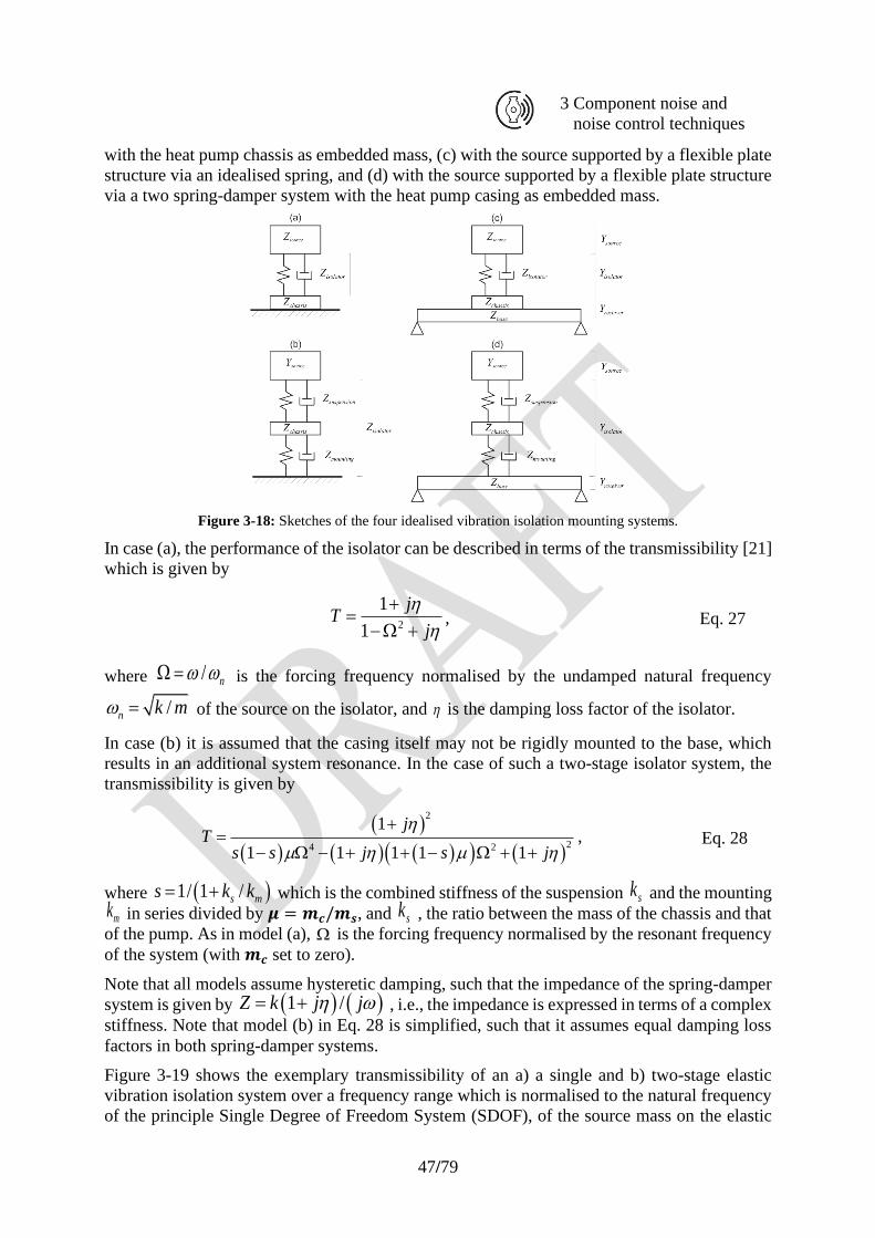
47/79



with the heat pump chassis as embedded mass, (c) with the source supported by a flexible plate

structure via an idealised spring, and (d) with the source supported by a flexible plate structure

via a two spring-damper system with the heat pump casing as embedded mass.

Figure 3-18: Sketches of the four idealised vibration isolation mounting systems.

In case (a), the performance of the isolator can be described in terms of the transmissibility [21]

which is given by

2

1

1

jT

j

+=

− +, Eq. 27

where / n = is the forcing frequency normalised by the undamped natural frequency

/n k m = of the source on the isolator, and is the damping loss factor of the isolator.

In case (b) it is assumed that the casing itself may not be rigidly mounted to the base, which

results in an additional system resonance. In the case of such a two-stage isolator system, the

transmissibility is given by

( )

( ) ( ) ( )( ) ( )

2

24 2

1

1 1 1 1 1

jT

s s j s j

+=

− − + + − + +, Eq. 28

where ( )1/ 1 /s ms k k= + which is the combined stiffness of the suspension sk and the mounting

mk in series divided by 𝝁 = 𝒎𝒄/𝒎𝒔, and sk , the ratio between the mass of the chassis and that

of the pump. As in model (a), is the forcing frequency normalised by the resonant frequency

of the system (with 𝒎𝒄 set to zero).

Note that all models assume hysteretic damping, such that the impedance of the spring-damper

system is given by ( ) ( )1 /Z k j j = + , i.e., the impedance is expressed in terms of a complex

stiffness. Note that model (b) in Eq. 28 is simplified, such that it assumes equal damping loss

factors in both spring-damper systems.

Figure 3-19 shows the exemplary transmissibility of an a) a single and b) two-stage elastic

vibration isolation system over a frequency range which is normalised to the natural frequency

of the principle Single Degree of Freedom System (SDOF), of the source mass on the elastic

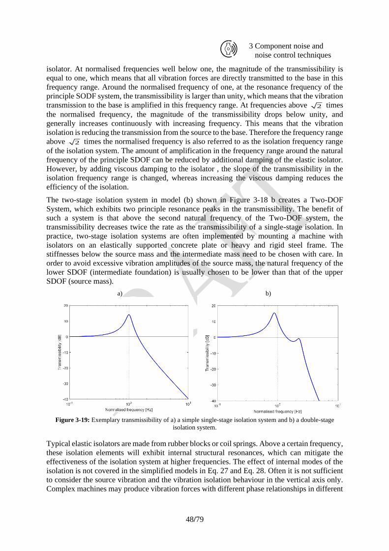
48/79



isolator. At normalised frequencies well below one, the magnitude of the transmissibility is

equal to one, which means that all vibration forces are directly transmitted to the base in this

frequency range. Around the normalised frequency of one, at the resonance frequency of the

principle SODF system, the transmissibility is larger than unity, which means that the vibration

transmission to the base is amplified in this frequency range. At frequencies above 2 times

the normalised frequency, the magnitude of the transmissibility drops below unity, and

generally increases continuously with increasing frequency. This means that the vibration

isolation is reducing the transmission from the source to the base. Therefore the frequency range

above 2 times the normalised frequency is also referred to as the isolation frequency range

of the isolation system. The amount of amplification in the frequency range around the natural

frequency of the principle SDOF can be reduced by additional damping of the elastic isolator.

However, by adding viscous damping to the isolator , the slope of the transmissibility in the

isolation frequency range is changed, whereas increasing the viscous damping reduces the

efficiency of the isolation.

The two-stage isolation system in model (b) shown in Figure 3-18 b creates a Two-DOF

System, which exhibits two principle resonance peaks in the transmissibility. The benefit of

such a system is that above the second natural frequency of the Two-DOF system, the

transmissibility decreases twice the rate as the transmissibility of a single-stage isolation. In

practice, two-stage isolation systems are often implemented by mounting a machine with

isolators on an elastically supported concrete plate or heavy and rigid steel frame. The

stiffnesses below the source mass and the intermediate mass need to be chosen with care. In

order to avoid excessive vibration amplitudes of the source mass, the natural frequency of the

lower SDOF (intermediate foundation) is usually chosen to be lower than that of the upper

SDOF (source mass).

a) b)

Figure 3-19: Exemplary transmissibility of a) a simple single-stage isolation system and b) a double-stage

isolation system.

Typical elastic isolators are made from rubber blocks or coil springs. Above a certain frequency,

these isolation elements will exhibit internal structural resonances, which can mitigate the

effectiveness of the isolation system at higher frequencies. The effect of internal modes of the

isolation is not covered in the simplified models in Eq. 27 and Eq. 28. Often it is not sufficient

to consider the source vibration and the vibration isolation behaviour in the vertical axis only.

Complex machines may produce vibration forces with different phase relationships in different

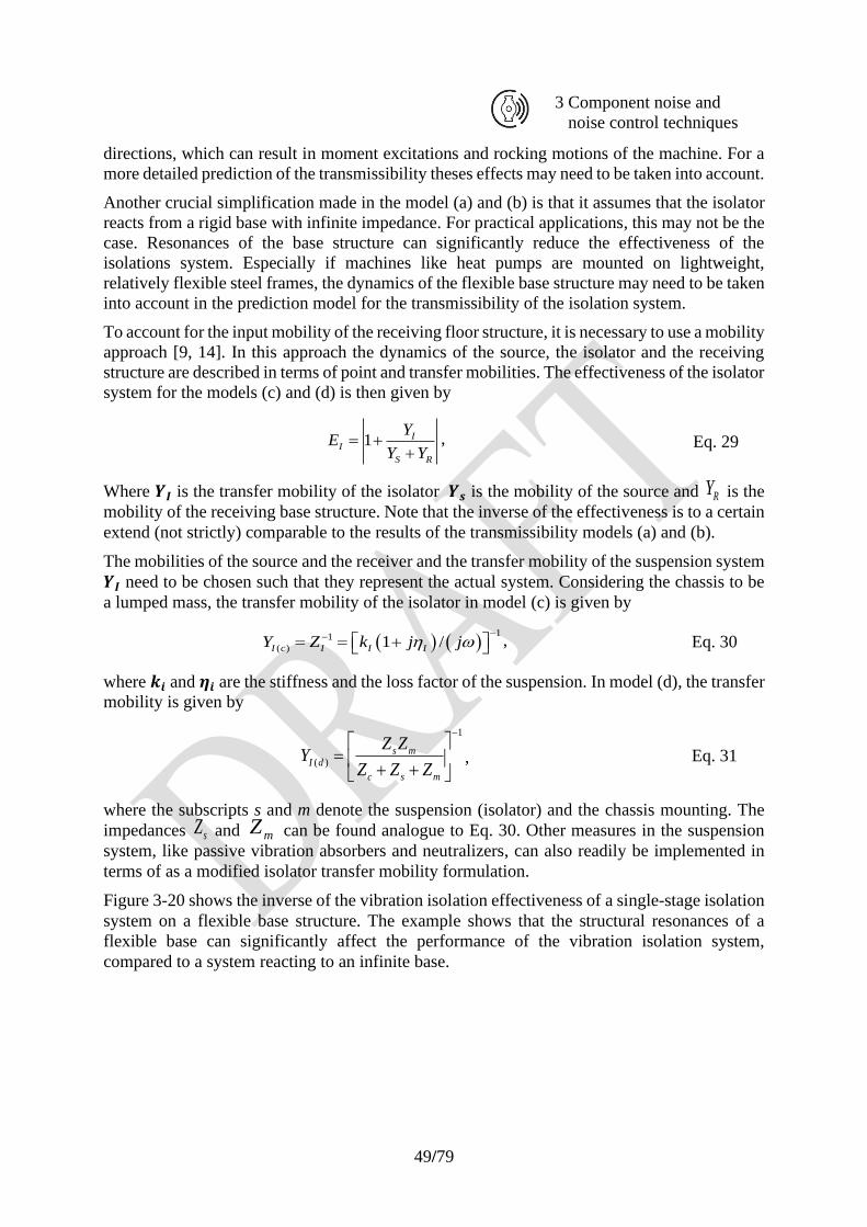
49/79



directions, which can result in moment excitations and rocking motions of the machine. For a

more detailed prediction of the transmissibility theses effects may need to be taken into account.

Another crucial simplification made in the model (a) and (b) is that it assumes that the isolator

reacts from a rigid base with infinite impedance. For practical applications, this may not be the

case. Resonances of the base structure can significantly reduce the effectiveness of the

isolations system. Especially if machines like heat pumps are mounted on lightweight,

relatively flexible steel frames, the dynamics of the flexible base structure may need to be taken

into account in the prediction model for the transmissibility of the isolation system.

To account for the input mobility of the receiving floor structure, it is necessary to use a mobility

approach [9, 14]. In this approach the dynamics of the source, the isolator and the receiving

structure are described in terms of point and transfer mobilities. The effectiveness of the isolator

system for the models (c) and (d) is then given by

1 II

S R

YE

Y Y= +

+, Eq. 29

Where 𝒀𝑰 is the transfer mobility of the isolator 𝒀𝒔 is the mobility of the source and RY is the

mobility of the receiving base structure. Note that the inverse of the effectiveness is to a certain

extend (not strictly) comparable to the results of the transmissibility models (a) and (b).

The mobilities of the source and the receiver and the transfer mobility of the suspension system

𝒀𝑰 need to be chosen such that they represent the actual system. Considering the chassis to be

a lumped mass, the transfer mobility of the isolator in model (c) is given by

( ) ( )11

( ) 1 /I c I I IY Z k j j −−= = + , Eq. 30

where 𝒌𝒊 and 𝜼𝒊 are the stiffness and the loss factor of the suspension. In model (d), the transfer

mobility is given by

1

( )s m

I d

c s m

Z ZY

Z Z Z

−

=

+ + , Eq. 31

where the subscripts s and m denote the suspension (isolator) and the chassis mounting. The

impedances sZ and mZ can be found analogue to Eq. 30. Other measures in the suspension

system, like passive vibration absorbers and neutralizers, can also readily be implemented in

terms of as a modified isolator transfer mobility formulation.

Figure 3-20 shows the inverse of the vibration isolation effectiveness of a single-stage isolation

system on a flexible base structure. The example shows that the structural resonances of a

flexible base can significantly affect the performance of the vibration isolation system,

compared to a system reacting to an infinite base.

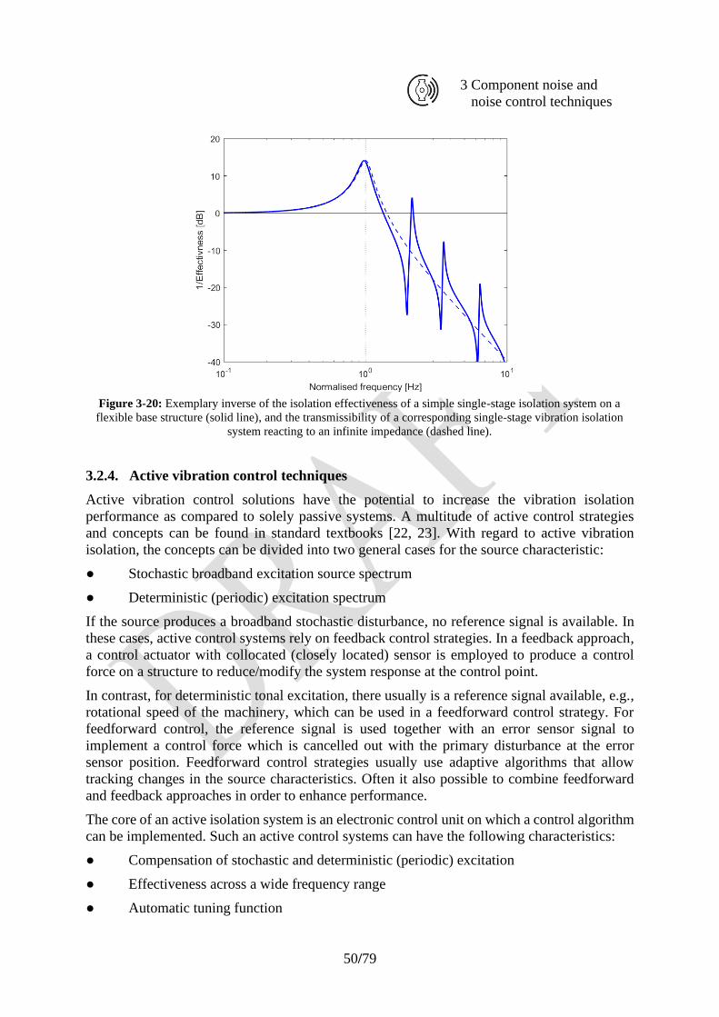
50/79



Figure 3-20: Exemplary inverse of the isolation effectiveness of a simple single-stage isolation system on a

flexible base structure (solid line), and the transmissibility of a corresponding single-stage vibration isolation

system reacting to an infinite impedance (dashed line).

3.2.4. Active vibration control techniques

Active vibration control solutions have the potential to increase the vibration isolation

performance as compared to solely passive systems. A multitude of active control strategies

and concepts can be found in standard textbooks [22, 23]. With regard to active vibration

isolation, the concepts can be divided into two general cases for the source characteristic:

● Stochastic broadband excitation source spectrum

● Deterministic (periodic) excitation spectrum

If the source produces a broadband stochastic disturbance, no reference signal is available. In

these cases, active control systems rely on feedback control strategies. In a feedback approach,

a control actuator with collocated (closely located) sensor is employed to produce a control

force on a structure to reduce/modify the system response at the control point.

In contrast, for deterministic tonal excitation, there usually is a reference signal available, e.g.,

rotational speed of the machinery, which can be used in a feedforward control strategy. For

feedforward control, the reference signal is used together with an error sensor signal to

implement a control force which is cancelled out with the primary disturbance at the error

sensor position. Feedforward control strategies usually use adaptive algorithms that allow

tracking changes in the source characteristics. Often it also possible to combine feedforward

and feedback approaches in order to enhance performance.

The core of an active isolation system is an electronic control unit on which a control algorithm

can be implemented. Such an active control systems can have the following characteristics:

● Compensation of stochastic and deterministic (periodic) excitation

● Effectiveness across a wide frequency range

● Automatic tuning function

51/79



● Possibility of controlling multiple actuators for the suppression of the overall vibration

induced by all mounting points.

● Possibility of addressing multiple critical forcing frequencies and critical response

resonance frequencies with a single actuator unit (controlled with a complex control

signal with multiple poles and zeros).

● Possibility of implementing multifunctionality, e.g., condition monitoring

The main benefit of an active isolation system is that it can adapt variations in the forcing

frequency, i.e., changes in the pumps’ operational conditions. With an appropriate system, this

adaptation could also track the forcing frequency during run-up phase, which may be

problematic with a purely passive or passive/adaptive system. In addition, actuator units are

able to provide higher actuation force at a lower total system weight than a purely passive

solution.

There are multiple concepts for adaptive/active vibration isolation solutions. As an example, an

actively tuneable bending beam vibration neutraliser was investigated in Ref. [24]. In practice,

the selection of an optimal control concept requires detailed simulation studies with more

detailed information of the actual source and receiver characteristics. While up to date there are

quite a few active mounting systems available for automotive applications, there seems to be

no off the-shelf active vibration isolation systems available for applications in heat pumps.

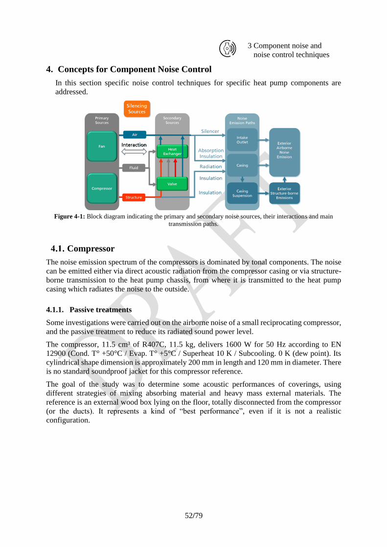
52/79



4. Concepts for Component Noise Control

In this section specific noise control techniques for specific heat pump components are

addressed.

Figure 4-1: Block diagram indicating the primary and secondary noise sources, their interactions and main

transmission paths.

Compressor

The noise emission spectrum of the compressors is dominated by tonal components. The noise

can be emitted either via direct acoustic radiation from the compressor casing or via structure-

borne transmission to the heat pump chassis, from where it is transmitted to the heat pump

casing which radiates the noise to the outside.

4.1.1. Passive treatments

Some investigations were carried out on the airborne noise of a small reciprocating compressor,

and the passive treatment to reduce its radiated sound power level.

The compressor, 11.5 cm³ of R407C, 11.5 kg, delivers 1600 W for 50 Hz according to EN

12900 (Cond. T° +50°C / Evap. T° +5°C / Superheat 10 K / Subcooling. 0 K (dew point). Its

cylindrical shape dimension is approximately 200 mm in length and 120 mm in diameter. There

is no standard soundproof jacket for this compressor reference.

The goal of the study was to determine some acoustic performances of coverings, using

different strategies of mixing absorbing material and heavy mass external materials. The

reference is an external wood box lying on the floor, totally disconnected from the compressor

(or the ducts). It represents a kind of “best performance”, even if it is not a realistic

configuration.

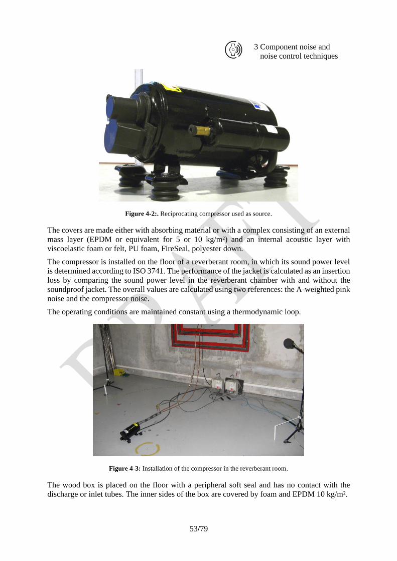
53/79



Figure 4-2:. Reciprocating compressor used as source.

The covers are made either with absorbing material or with a complex consisting of an external

mass layer (EPDM or equivalent for 5 or 10 kg/m²) and an internal acoustic layer with

viscoelastic foam or felt, PU foam, FireSeal, polyester down.

The compressor is installed on the floor of a reverberant room, in which its sound power level

is determined according to ISO 3741. The performance of the jacket is calculated as an insertion

loss by comparing the sound power level in the reverberant chamber with and without the

soundproof jacket. The overall values are calculated using two references: the A-weighted pink

noise and the compressor noise.

The operating conditions are maintained constant using a thermodynamic loop.

Figure 4-3: Installation of the compressor in the reverberant room.

The wood box is placed on the floor with a peripheral soft seal and has no contact with the

discharge or inlet tubes. The inner sides of the box are covered by foam and EPDM 10 kg/m².

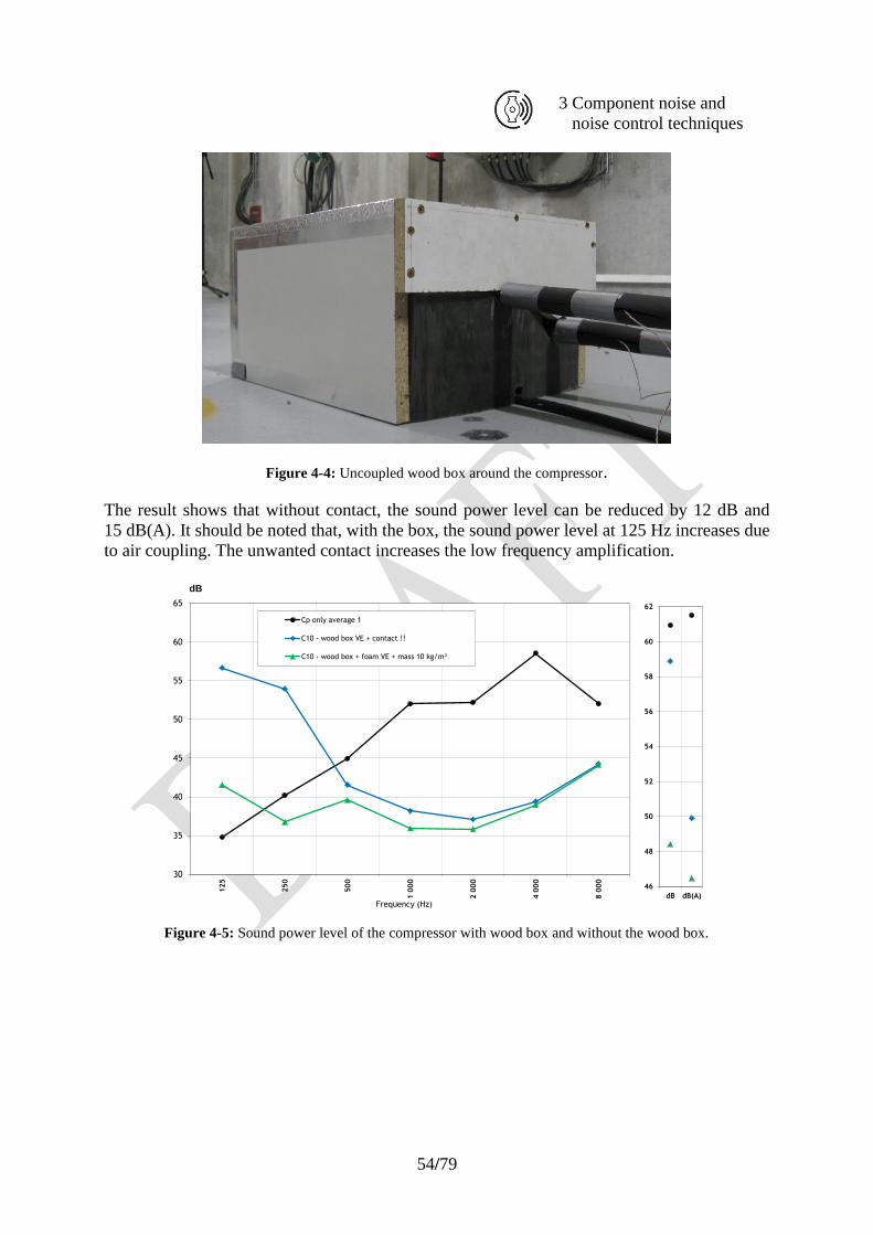
54/79



Figure 4-4: Uncoupled wood box around the compressor.

The result shows that without contact, the sound power level can be reduced by 12 dB and

15 dB(A). It should be noted that, with the box, the sound power level at 125 Hz increases due

to air coupling. The unwanted contact increases the low frequency amplification.

Figure 4-5: Sound power level of the compressor with wood box and without the wood box.

30

35

40

45

50

55

60

65

125

250

500

1 0

00

2 0

00

4 0

00

8 0

00

Frequency (Hz)

Cp only average 1

C10 - wood box VE + contact !!

C10 - wood box + foam VE + mass 10 kg/m²

46

48

50

52

54

56

58

60

62

dB dB(A)

dB

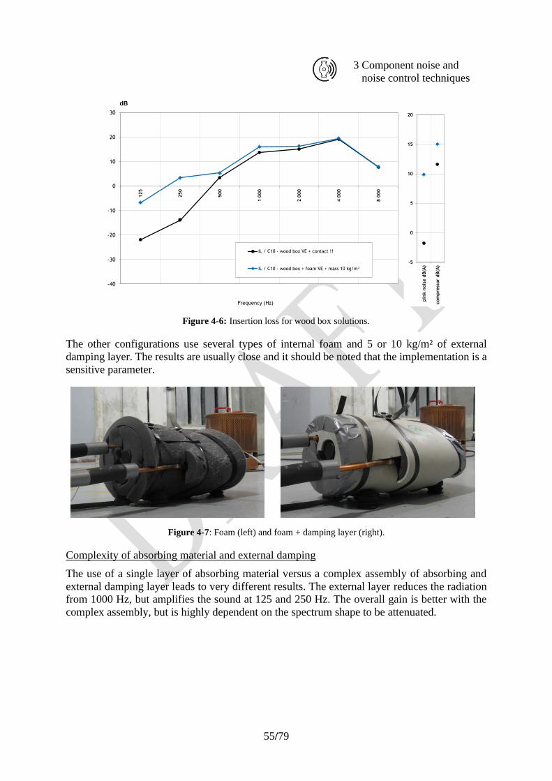
55/79



Figure 4-6: Insertion loss for wood box solutions.

The other configurations use several types of internal foam and 5 or 10 kg/m² of external

damping layer. The results are usually close and it should be noted that the implementation is a

sensitive parameter.

Figure 4-7: Foam (left) and foam + damping layer (right).

Complexity of absorbing material and external damping

The use of a single layer of absorbing material versus a complex assembly of absorbing and

external damping layer leads to very different results. The external layer reduces the radiation

from 1000 Hz, but amplifies the sound at 125 and 250 Hz. The overall gain is better with the

complex assembly, but is highly dependent on the spectrum shape to be attenuated.

-40

-30

-20

-10

0

10

20

30

125

250

500

1 0

00

2 0

00

4 0

00

8 0

00

Frequency (Hz)

IL / C10 - wood box VE + contact !!

IL / C10 - wood box + foam VE + mass 10 kg/m²

-5

0

5

10

15

20

pin

k n

ois

e d

B(A

)

com

pre

ssor

dB(A

)

dB

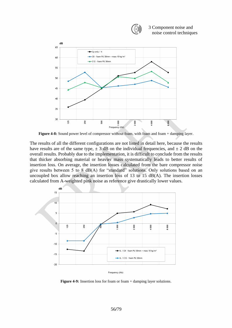
56/79



Figure 4-8: Sound power level of compressor without foam, with foam and foam + damping layer.

The results of all the different configurations are not listed in detail here, because the results

have results are of the same type, ± 3 dB on the individual frequencies, and ± 2 dB on the

overall results. Probably due to the implementation, it is difficult to conclude from the results

that thicker absorbing material or heavier mass systematically leads to better results of

insertion loss. On average, the insertion losses calculated from the bare compressor noise

give results between 5 to 8 dB(A) for “standard” solutions. Only solutions based on an

uncoupled box allow reaching an insertion loss of 13 to 15 dB(A). The insertion losses

calculated from A-weighted pink noise as reference give drastically lower values.

Figure 4-9: Insertion loss for foam or foam + damping layer solutions.

30

35

40

45

50

55

60

65

125

250

500

1 0

00

2 0

00

4 0

00

8 0

00

Frequency (Hz)

Cp only / 4

C8 - foam PU 30mm + mass 10 kg/m²

C12 - foam PU 30mm

54

55

56

57

58

59

60

61

62

dB dB(A)

dB

-20

-15

-10

-5

0

5

10

15

125

250

500

1 0

00

2 0

00

4 0

00

8 0

00

Frequency (Hz)

IL / C8 - foam PU 30mm + mass 10 kg/m²

IL / C12 - foam PU 30mm

2

3

4

5

6

7

8

pin

k n

ois

e d

B(A

)

com

pre

ssor

dB(A

)

dB

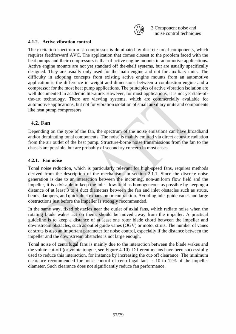
57/79



4.1.2. Active vibration control

The excitation spectrum of a compressor is dominated by discrete tonal components, which

requires feedforward AVC. The application that comes closest to the problem faced with the

heat pumps and their compressors is that of active engine mounts in automotive applications.

Active engine mounts are not yet standard off the-shelf systems, but are usually specifically

designed. They are usually only used for the main engine and not for auxiliary units. The

difficulty in adopting concepts from existing active engine mounts from an automotive

application is the difference in weight and dimensions between a combustion engine and a

compressor for the most heat pump applications. The principles of active vibration isolation are

well documented in academic literature. However, for most applications, it is not yet state-of-

the-art technology. There are viewing systems, which are commercially available for

automotive applications, but not for vibration isolation of small auxiliary units and components

like heat pump compressors.

Fan

Depending on the type of the fan, the spectrum of the noise emissions can have broadband

and/or dominating tonal components. The noise is mainly emitted via direct acoustic radiation

from the air outlet of the heat pump. Structure-borne noise transmissions from the fan to the

chassis are possible, but are probably of secondary concern in most cases.

4.2.1. Fan noise

Tonal noise reduction, which is particularly relevant for high-speed fans, requires methods

derived from the description of the mechanisms in section 2.1.1. Since the discrete noise

generation is due to an interaction between the incoming, non-uniform flow field and the

impeller, it is advisable to keep the inlet flow field as homogeneous as possible by keeping a

distance of at least 3 to 4 duct diameters between the fan and inlet obstacles such as struts,

bends, dampers, and quick duct expansion or contraction. Avoiding inlet guide vanes and large

obstructions just before the impeller is strongly recommended.

In the same way, fixed obstacles near the outlet of axial fans, which radiate noise when the

rotating blade wakes act on them, should be moved away from the impeller. A practical

guideline is to keep a distance of at least one rotor blade chord between the impeller and

downstream obstacles, such as outlet guide vanes (OGV) or motor struts. The number of vanes

or struts is also an important parameter for noise control, especially if the distance between the

impeller and the downstream obstacles is not large enough.

Tonal noise of centrifugal fans is mainly due to the interaction between the blade wakes and

the volute cut-off (or volute tongue, see Figure 4-10). Different means have been successfully

used to reduce this interaction, for instance by increasing the cut-off clearance. The minimum

clearance recommended for noise control of centrifugal fans is 10 to 12% of the impeller

diameter. Such clearance does not significantly reduce fan performance.

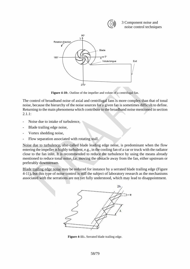
58/79



Figure 4-10:. Outline of the impeller and volute of a centrifugal fan.

The control of broadband noise of axial and centrifugal fans is more complex than that of tonal

noise, because the hierarchy of the noise sources for a given fan is sometimes difficult to define.

Returning to the main phenomena which contribute to the broadband noise mentioned in section

2.1.1:

- Noise due to intake of turbulence,

- Blade trailing edge noise,

- Vortex shedding noise,

- Flow separation associated with rotating stall.

Noise due to turbulence, also called blade leading edge noise, is predominant when the flow

entering the impeller is highly turbulent, e.g., in the cooling fan of a car or truck with the radiator

close to the fan inlet. It is recommended to reduce the turbulence by using the means already

mentioned to reduce tonal noise, i.e. moving the obstacle away from the fan, either upstream or

preferably downstream.

Blade trailing edge noise may be reduced for instance by a serrated blade trailing edge (Figure

4-11), but this type of noise control is still the subject of laboratory research as the mechanisms

associated with the serrations are not yet fully understood, which may lead to disappointment.

Figure 4-11:. Serrated blade trailing edge.

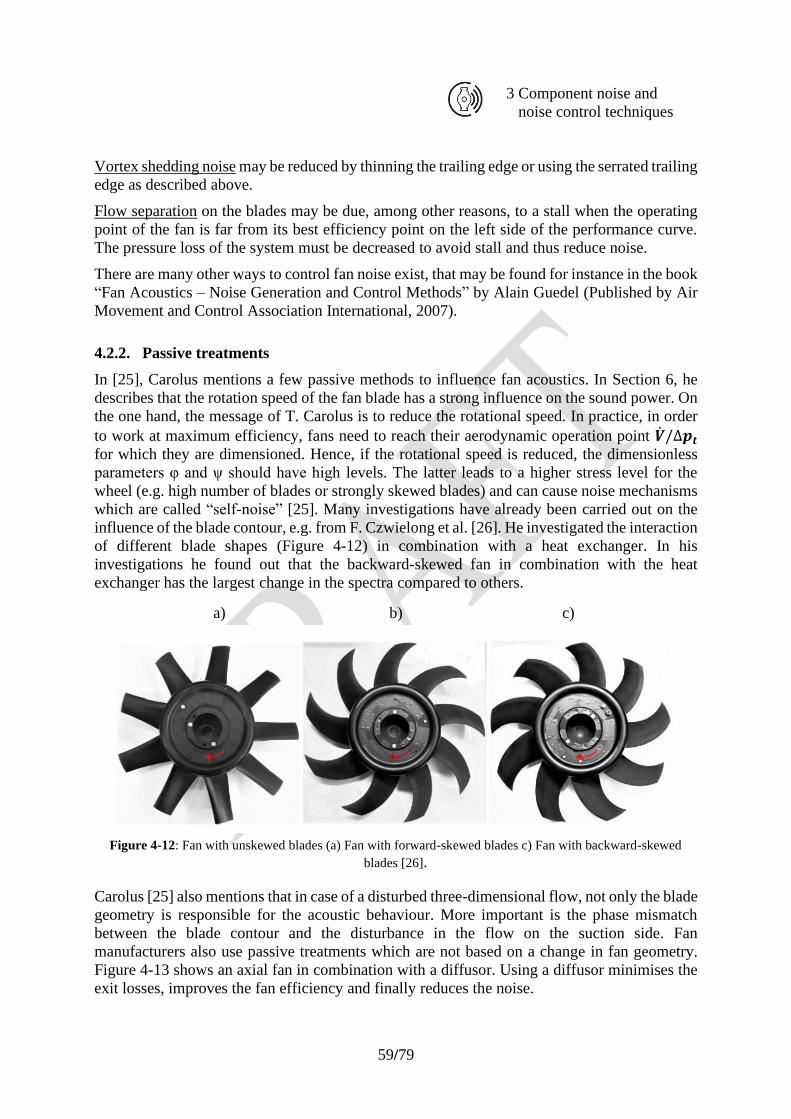
59/79



Vortex shedding noise may be reduced by thinning the trailing edge or using the serrated trailing

edge as described above.

Flow separation on the blades may be due, among other reasons, to a stall when the operating

point of the fan is far from its best efficiency point on the left side of the performance curve.

The pressure loss of the system must be decreased to avoid stall and thus reduce noise.

There are many other ways to control fan noise exist, that may be found for instance in the book

“Fan Acoustics – Noise Generation and Control Methods” by Alain Guedel (Published by Air

Movement and Control Association International, 2007).


In [25], Carolus mentions a few passive methods to influence fan acoustics. In Section 6, he

describes that the rotation speed of the fan blade has a strong influence on the sound power. On

the one hand, the message of T. Carolus is to reduce the rotational speed. In practice, in order

to work at maximum efficiency, fans need to reach their aerodynamic operation point ��/∆𝒑𝒕

for which they are dimensioned. Hence, if the rotational speed is reduced, the dimensionless

parameters φ and ψ should have high levels. The latter leads to a higher stress level for the

wheel (e.g. high number of blades or strongly skewed blades) and can cause noise mechanisms

which are called “self-noise” [25]. Many investigations have already been carried out on the

influence of the blade contour, e.g. from F. Czwielong et al. [26]. He investigated the interaction

of different blade shapes (Figure 4-12) in combination with a heat exchanger. In his

investigations he found out that the backward-skewed fan in combination with the heat

exchanger has the largest change in the spectra compared to others.

a) b) c)

Figure 4-12: Fan with unskewed blades (a) Fan with forward-skewed blades c) Fan with backward-skewed

blades [26].

Carolus [25] also mentions that in case of a disturbed three-dimensional flow, not only the blade

geometry is responsible for the acoustic behaviour. More important is the phase mismatch

between the blade contour and the disturbance in the flow on the suction side. Fan

manufacturers also use passive treatments which are not based on a change in fan geometry.

Figure 4-13 shows an axial fan in combination with a diffusor. Using a diffusor minimises the

exit losses, improves the fan efficiency and finally reduces the noise.

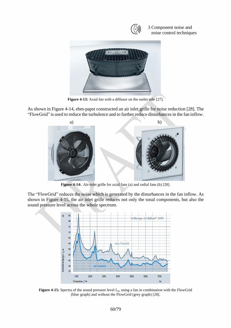
60/79



Figure 4-13: Axial fan with a diffusor on the outlet side [27].

As shown in Figure 4-14, ebm-papst constructed an air inlet grille for noise reduction [28]. The

“FlowGrid” is used to reduce the turbulence and to further reduce disturbances in the fan inflow.

a) b)

Figure 4-14:. Air-inlet grille for axial fans (a) and radial fans (b) [28].

The “FlowGrid” reduces the noise which is generated by the disturbances in the fan inflow. As

shown in Figure 4-15, the air inlet grille reduces not only the tonal components, but also the

sound pressure level across the whole spectrum.

Figure 4-15: Spectra of the sound pressure level Lp, using a fan in combination with the FlowGrid

(blue graph) and without the FlowGrid (grey graph) [28].

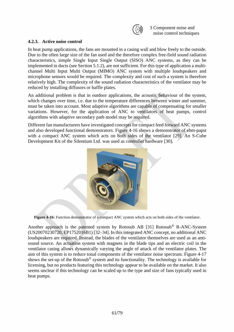
61/79



4.2.3. Active noise control

In heat pump applications, the fans are mounted in a casing wall and blow freely to the outside.

Due to the often large size of the fan used and the therefore complex free-field sound radiation

characteristics, simple Single Input Single Output (SISO) ANC systems, as they can be

implemented in ducts (see Section 5.1.2), are not sufficient. For this type of application a multi-

channel Multi Input Multi Output (MIMO) ANC system with multiple loudspeakers and

microphone sensors would be required. The complexity and cost of such a system is therefore

relatively high. The complexity of the sound radiation characteristics of the ventilator may be

reduced by installing diffusors or baffle plates.

An additional problem is that in outdoor applications, the acoustic behaviour of the system,

which changes over time, i.e. due to the temperature differences between winter and summer,

must be taken into account. Most adaptive algorithms are capable of compensating for smaller

variations. However, for the application of ANC to ventilators of heat pumps, control

algorithms with adaptive secondary path model may be required.

Different fan manufacturers have investigated concepts for compact feed forward ANC systems

and also developed functional demonstrators. Figure 4-16 shows a demonstrator of ebm-papst

with a compact ANC system which acts on both sides of the ventilator [29]. An S-Cube

Development Kit of the Silentium Ltd. was used as controller hardware [30].

Figure 4-16: Function demonstrator of a compact ANC system which acts on both sides of the ventilator.

Another approach is the patented system by Rotosub AB [31] Rotosub® R-ANC-System

(US20070230720, EP1752016B1) [32–34]. In this integrated ANC concept, no additional ANC

loudspeakers are required. Instead, the blades of the ventilator themselves are used as an anti-

sound source. An actuation system with magnets in the blade tips and an electric coil in the

ventilator casing allows dynamically varying the angle of attack of the ventilator plates. The

aim of this system is to reduce tonal components of the ventilator noise spectrum. Figure 4-17

shows the set-up of the Rotosub® system and its functionality. The technology is available for

licensing, but no products featuring this technology appear to be available on the market. It also

seems unclear if this technology can be scaled up to the type and size of fans typically used in

heat pumps.

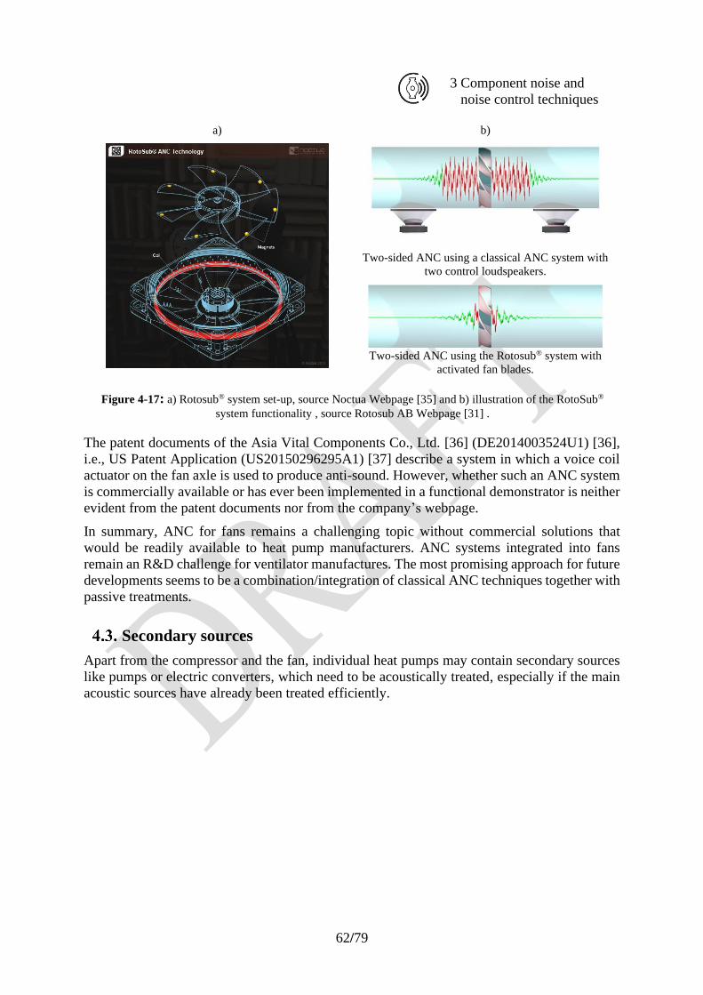
62/79



a)

b)

Two-sided ANC using a classical ANC system with

two control loudspeakers.

Two-sided ANC using the Rotosub® system with

activated fan blades.

Figure 4-17: a) Rotosub® system set-up, source Noctua Webpage [35] and b) illustration of the RotoSub®

system functionality , source Rotosub AB Webpage [31] .

The patent documents of the Asia Vital Components Co., Ltd. [36] (DE2014003524U1) [36],

i.e., US Patent Application (US20150296295A1) [37] describe a system in which a voice coil

actuator on the fan axle is used to produce anti-sound. However, whether such an ANC system

is commercially available or has ever been implemented in a functional demonstrator is neither

evident from the patent documents nor from the company’s webpage.

In summary, ANC for fans remains a challenging topic without commercial solutions that

would be readily available to heat pump manufacturers. ANC systems integrated into fans

remain an R&D challenge for ventilator manufactures. The most promising approach for future

developments seems to be a combination/integration of classical ANC techniques together with

passive treatments.

Secondary sources

Apart from the compressor and the fan, individual heat pumps may contain secondary sources

like pumps or electric converters, which need to be acoustically treated, especially if the main

acoustic sources have already been treated efficiently.

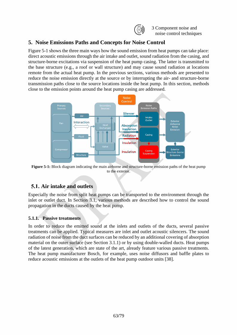
63/79



5. Noise Emissions Paths and Concepts for Noise Control

Figure 5-1 shows the three main ways how the sound emission from heat pumps can take place:

direct acoustic emissions through the air intake and outlet, sound radiation from the casing, and

structure-borne excitations via suspension of the heat pump casing. The latter is transmitted to

the base structure (e.g., a roof or wall structure) and may cause sound radiation at locations

remote from the actual heat pump. In the previous sections, various methods are presented to

reduce the noise emission directly at the source or by interrupting the air- and structure-borne

transmission paths close to the source locations inside the heat pump. In this section, methods

close to the emission points around the heat pump casing are addressed.

Figure 5-1: Block diagram indicating the main airborne and structure-borne emission paths of the heat pump

to the exterior.

Air intake and outlets

Especially the noise from split heat pumps can be transported to the environment through the

inlet or outlet duct. In Section 3.1, various methods are described how to control the sound

propagation in the ducts caused by the heat pump.


In order to reduce the emitted sound at the inlets and outlets of the ducts, several passive

treatments can be applied. Typical measures are inlet and outlet acoustic silencers. The sound

radiation of noise from the duct surfaces can be reduced by an additional covering of absorption

material on the outer surface (see Section 3.1.1) or by using double-walled ducts. Heat pumps

of the latest generation, which are state of the art, already feature various passive treatments.

The heat pump manufacturer Bosch, for example, uses noise diffusors and baffle plates to

reduce acoustic emissions at the outlets of the heat pump outdoor units [38].

64/79



Figure 5-2: Bosch Compress 7400i AW with noise diffusor at the outlet [38],[39].

5.1.2. Active noise control

Most exhaust and ventilation systems comprise specifically designed silencers and absorbers to

reduce noise emission. As discussed in Section 3.1.2, conventional silencers usually comprise

porous absorbers and/or acoustics resonators. For applications with weight restrictions and

where installation space is limited, active noise control (ANC) approaches can be an alternative.

Some general features of ANC are described in Section 3.1.4. Below the so-called cut-off

frequency of higher order duct modes, which depends on the geometry of the duct cross section,

the sound field in inlet and outlet ducts may be described as plane waves with equal pressure

distribution across the duct cross section. Below the cut-off frequency, duct ANC-systems can

be implemented as relatively simple SISO ANC systems. Similar to the discussion in Section

3.1.4, ANC for duct applications may be divided into feedforward and feedback ANC

approaches.

Feed forward ANC systems for inlet and outlet ducts require an error and reference sensor

(physical or virtual), a control transducer and a controller. Figure 5-3 illustrates the basic setup

of a feedforward ANC System in a duct. A reference sensor (microphone) is used to sense a

sound wave ‘upstream’ from an control loudspeaker location. This reference signal is filtered

via a controller transfer function and played back via the control loudspeaker such that the

primary and secondary sound fields destructively interact and cancel each other out. A

challenge is that the controller transfer function needed is not known. In very early concepts of

ANC, the magnitude and phase of single tones were adjusted manually in order to achieve the

desired cancellation effect at the control loudspeaker. Today, in most practical applications, an

adaptive control algorithm is implemented on a digital signal processor (DSP). Apart from the

digital controller, such systems also require an ‘downstream’ error signal, which the system

tries to minimise. Most often a so-called LMS algorithm or variations of it are used for online

system identification and adaptation of the controller transfer function. Depending on the

application, feedforward ANC systems may be implemented to reduce low frequency noise or

to cancel out only tonal noise components (engine or fan orders).

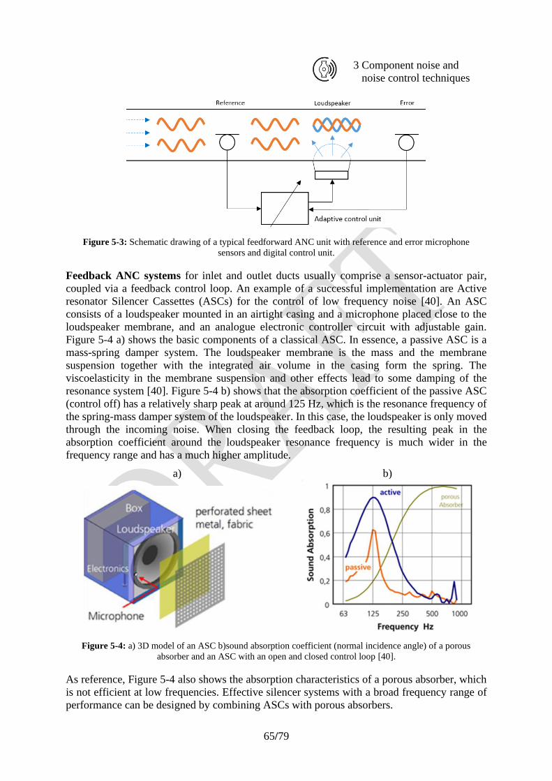
65/79



Figure 5-3: Schematic drawing of a typical feedforward ANC unit with reference and error microphone

sensors and digital control unit.

Feedback ANC systems for inlet and outlet ducts usually comprise a sensor-actuator pair,

coupled via a feedback control loop. An example of a successful implementation are Active

resonator Silencer Cassettes (ASCs) for the control of low frequency noise [40]. An ASC

consists of a loudspeaker mounted in an airtight casing and a microphone placed close to the

loudspeaker membrane, and an analogue electronic controller circuit with adjustable gain.

Figure 5-4 a) shows the basic components of a classical ASC. In essence, a passive ASC is a

mass-spring damper system. The loudspeaker membrane is the mass and the membrane

suspension together with the integrated air volume in the casing form the spring. The

viscoelasticity in the membrane suspension and other effects lead to some damping of the

resonance system [40]. Figure 5-4 b) shows that the absorption coefficient of the passive ASC

(control off) has a relatively sharp peak at around 125 Hz, which is the resonance frequency of

the spring-mass damper system of the loudspeaker. In this case, the loudspeaker is only moved

through the incoming noise. When closing the feedback loop, the resulting peak in the

absorption coefficient around the loudspeaker resonance frequency is much wider in the

frequency range and has a much higher amplitude.

a) b)

Figure 5-4: a) 3D model of an ASC b)sound absorption coefficient (normal incidence angle) of a porous

absorber and an ASC with an open and closed control loop [40].

As reference, Figure 5-4 also shows the absorption characteristics of a porous absorber, which

is not efficient at low frequencies. Effective silencer systems with a broad frequency range of

performance can be designed by combining ASCs with porous absorbers.

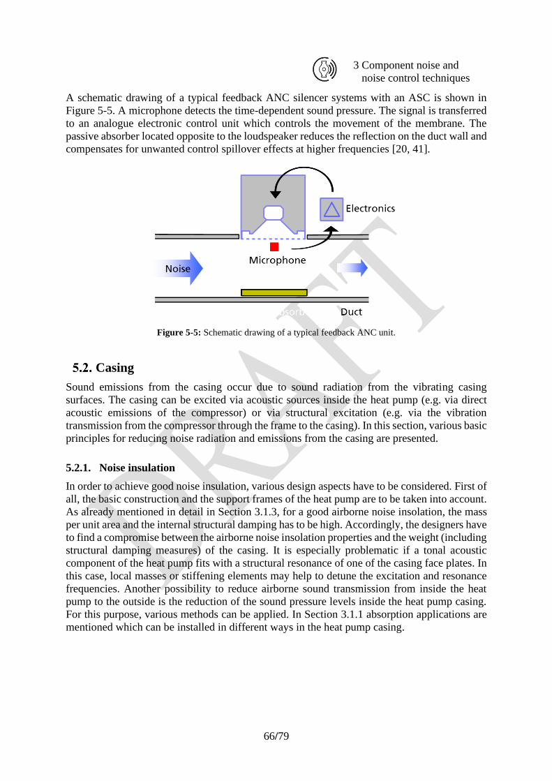
66/79



A schematic drawing of a typical feedback ANC silencer systems with an ASC is shown in

Figure 5-5. A microphone detects the time-dependent sound pressure. The signal is transferred

to an analogue electronic control unit which controls the movement of the membrane. The

passive absorber located opposite to the loudspeaker reduces the reflection on the duct wall and

compensates for unwanted control spillover effects at higher frequencies [20, 41].

Figure 5-5: Schematic drawing of a typical feedback ANC unit.

Casing

Sound emissions from the casing occur due to sound radiation from the vibrating casing

surfaces. The casing can be excited via acoustic sources inside the heat pump (e.g. via direct

acoustic emissions of the compressor) or via structural excitation (e.g. via the vibration

transmission from the compressor through the frame to the casing). In this section, various basic

principles for reducing noise radiation and emissions from the casing are presented.

5.2.1. Noise insulation

In order to achieve good noise insulation, various design aspects have to be considered. First of

all, the basic construction and the support frames of the heat pump are to be taken into account.

As already mentioned in detail in Section 3.1.3, for a good airborne noise insolation, the mass

per unit area and the internal structural damping has to be high. Accordingly, the designers have

to find a compromise between the airborne noise insolation properties and the weight (including

structural damping measures) of the casing. It is especially problematic if a tonal acoustic

component of the heat pump fits with a structural resonance of one of the casing face plates. In

this case, local masses or stiffening elements may help to detune the excitation and resonance

frequencies. Another possibility to reduce airborne sound transmission from inside the heat

pump to the outside is the reduction of the sound pressure levels inside the heat pump casing.

For this purpose, various methods can be applied. In Section 3.1.1 absorption applications are

mentioned which can be installed in different ways in the heat pump casing.

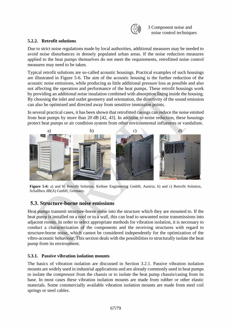
67/79



5.2.2. Retrofit solutions

Due to strict noise regulations made by local authorities, additional measures may be needed to

avoid noise disturbances in densely populated urban areas. If the noise reduction measures

applied to the heat pumps themselves do not meet the requirements, retrofitted noise control

measures may need to be taken.

Typical retrofit solutions are so-called acoustic housings. Practical examples of such housings

are illustrated in Figure 5-6. The aim of the acoustic housing is the further reduction of the

acoustic noise emissions, while producing as little additional pressure loss as possible and also

not affecting the operation and performance of the heat pumps. These retrofit housings work

by providing an additional noise insulation combined with absorption lining inside the housing.

By choosing the inlet and outlet geometry and orientation, the directivity of the sound emission

can also be optimised and directed away from sensitive immission points.

In several practical cases, it has been shown that retrofitted casings can reduce the noise emitted

from heat pumps by more than 20 dB [42, 43]. In addition to noise reduction, these housings

protect heat pumps or air condition system from other environmental influences or vandalism.

a) b) c) d)

Figure 5-6: a) and b) Retrofit Solution, Kellner Engineering GmbH, Austria; b) and c) Retrofit Solution,

Schallbox dB(A) GmbH, Germany.

Structure-borne noise emissions

Heat pumps transmit structure-borne noise into the structure which they are mounted to. If the

heat pump is installed on a roof or to a wall, this can lead to unwanted noise transmissions into

adjacent rooms. In order to select appropriate methods for vibration isolation, it is necessary to

conduct a characterization of the components and the receiving structures with regard to

structure-borne noise, which cannot be considered independently for the optimization of the

vibro-acoustic behaviour. This section deals with the possibilities to structurally isolate the heat

pump from its environment.

5.3.1. Passive vibration isolation mounts

The basics of vibration isolation are discussed in Section 3.2.1. Passive vibration isolation

mounts are widely used in industrial applications and are already commonly used in heat pumps

to isolate the compressor from the chassis or to isolate the heat pump chassis/casing from its

base. In most cases these vibration isolation mounts are made from rubber or other elastic

materials. Some commercially available vibration isolation mounts are made from steel coil

springs or steel cables.

68/79



As discussed in Section 3.2.1, when choosing vibration isolation mounts, it is important to know

the static and dynamic loads of the source and the vibration isolation frequency range of interest.

The vibration isolation mounts must be selected such that they can withstand the static and

dynamic loads and with respect to the resulting mass-spring system resonance frequency. If the

base on which the source is mounted cannot be considered as sufficiently stiff/heavy (e.g. in

the cases where heat pumps are mounted on a metal frame or grid), it is also important to

consider the interaction between the source, the vibration isolation and the base structure.

Depending on the requirements of the application, isolation systems can comprise multiple

elastic components and be combined with vibration absorbers and vibration neutralizers.

Vibration isolation mounts need to be carefully selected for each individual application to

guarantee optimal vibration isolation performance. A discussion on how to model and design

the vibration transmissibility of different isolation systems is provided in section 3.2.3.

5.3.2. Adaptive and active mounts

Most active vibration isolation systems available off-the-shelf are designed to isolate sensitive

machinery parts from the base vibrations of the supporting structure. For these applications, a

variety of active mounting systems is available such as workstations, benchtop platforms,

breadboards, equipment platforms, and vibration-free islands.

The application that comes closest to the problem faced with heat pumps and their compressors

is that of active engine mounts in automotive applications. Active engine mounts are not yet

standard off-the-shelf-systems but are mostly designed specifically for a particular application

[44, 45]. It may be possible to adopt concepts of existing active engine mounts from an

automotive application where the weight and dimensions of the vibrating component are similar

to those of a conventional combustion engine. Another field of application of active engine

mounts is the use in heavy ship diesel engines [46]. Here, too, the solutions are usually tailored

to the specific application which is possible due to the high overall cost of the machine.

It can be summarised that the principle of active vibration isolation is well documented in the

academic literature but is not yet state-of-the-art technology which is commercially available

as a generic product. Currently, there seems to exist no generic off-the-shelf solution which

would guarantee to meet the requirements of applications in heat pumps.

5.3.3. Mountings, pipes

It is important to avoid vibration transmission bridges from pipes to the chassis/casing.

Therefore pipes and cables should be fastened with appropriate elastic mounts.

69/79



6. Effect of Operating Conditions of Heat Pumps on Acoustic Behaviour

The operating conditions, especially transient operation modes influence the heat pumps

acoustic behaviour and are an important aspect in the control of noise from heat pumps. In the

Annex 51 Task 4 report »Analysis of the Effect of Operating Conditions of Heat Pumps on

Acoustic Behaviour« this topic is addressed in greater detail. A short abstract of the Annex 51

Task 4 report is provided below:

The Annex 51 Task 4 report deals with tools that allow the modelling of the acoustic emissions

of a heat pump as a function of its operating state. The noise emissions resulting from transient

operations are examined, beginning with a description of the physical processes likely to

produce the most obvious or bothersome noises, before describing them by order of time scale.

Where possible, recommendations on how to reduce the influence of those acoustic emissions

are discussed. Finally, the dependency on the type of heat source and the temperature and load

levels are examined.

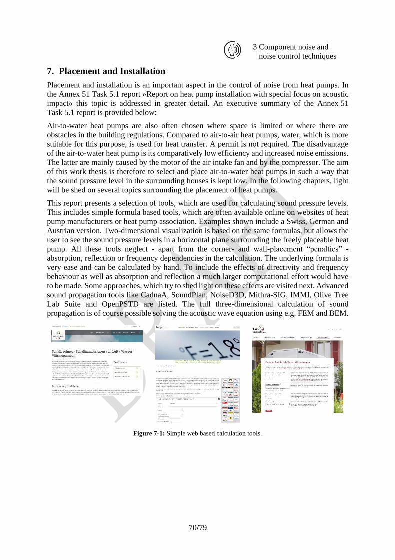
70/79



7. Placement and Installation

Placement and installation is an important aspect in the control of noise from heat pumps. In

the Annex 51 Task 5.1 report »Report on heat pump installation with special focus on acoustic

impact« this topic is addressed in greater detail. An executive summary of the Annex 51

Task 5.1 report is provided below:

Air-to-water heat pumps are also often chosen where space is limited or where there are

obstacles in the building regulations. Compared to air-to-air heat pumps, water, which is more

suitable for this purpose, is used for heat transfer. A permit is not required. The disadvantage

of the air-to-water heat pump is its comparatively low efficiency and increased noise emissions.

The latter are mainly caused by the motor of the air intake fan and by the compressor. The aim

of this work thesis is therefore to select and place air-to-water heat pumps in such a way that

the sound pressure level in the surrounding houses is kept low. In the following chapters, light

will be shed on several topics surrounding the placement of heat pumps.

This report presents a selection of tools, which are used for calculating sound pressure levels.

This includes simple formula based tools, which are often available online on websites of heat

pump manufacturers or heat pump association. Examples shown include a Swiss, German and

Austrian version. Two-dimensional visualization is based on the same formulas, but allows the

user to see the sound pressure levels in a horizontal plane surrounding the freely placeable heat

pump. All these tools neglect - apart from the corner- and wall-placement “penalties” -

absorption, reflection or frequency dependencies in the calculation. The underlying formula is

very ease and can be calculated by hand. To include the effects of directivity and frequency

behaviour as well as absorption and reflection a much larger computational effort would have

to be made. Some approaches, which try to shed light on these effects are visited next. Advanced

sound propagation tools like CadnaA, SoundPlan, NoiseD3D, Mithra-SIG, IMMI, Olive Tree

Lab Suite and OpenPSTD are listed. The full three-dimensional calculation of sound

propagation is of course possible solving the acoustic wave equation using e.g. FEM and BEM.

Figure 7-1: Simple web based calculation tools.

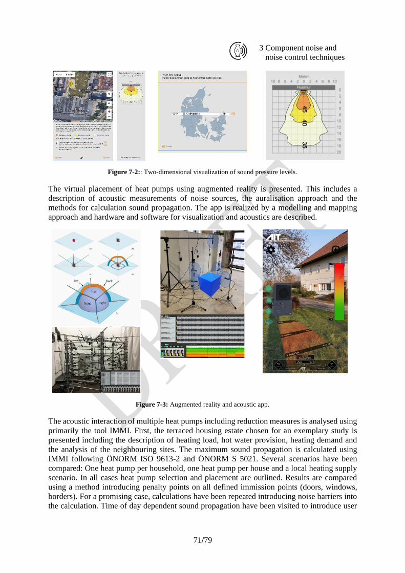
71/79



Figure 7-2:: Two-dimensional visualization of sound pressure levels.

The virtual placement of heat pumps using augmented reality is presented. This includes a

description of acoustic measurements of noise sources, the auralisation approach and the

methods for calculation sound propagation. The app is realized by a modelling and mapping

approach and hardware and software for visualization and acoustics are described.

Figure 7-3: Augmented reality and acoustic app.

The acoustic interaction of multiple heat pumps including reduction measures is analysed using

primarily the tool IMMI. First, the terraced housing estate chosen for an exemplary study is

presented including the description of heating load, hot water provision, heating demand and

the analysis of the neighbouring sites. The maximum sound propagation is calculated using

IMMI following ÖNORM ISO 9613-2 and ÖNORM S 5021. Several scenarios have been

compared: One heat pump per household, one heat pump per house and a local heating supply

scenario. In all cases heat pump selection and placement are outlined. Results are compared

using a method introducing penalty points on all defined immission points (doors, windows,

borders). For a promising case, calculations have been repeated introducing noise barriers into

the calculation. Time of day dependent sound propagation have been visited to introduce user

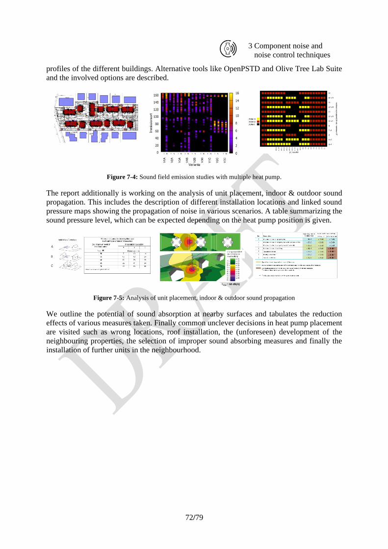
72/79



profiles of the different buildings. Alternative tools like OpenPSTD and Olive Tree Lab Suite

and the involved options are described.

Figure 7-4: Sound field emission studies with multiple heat pump.

The report additionally is working on the analysis of unit placement, indoor & outdoor sound

propagation. This includes the description of different installation locations and linked sound

pressure maps showing the propagation of noise in various scenarios. A table summarizing the

sound pressure level, which can be expected depending on the heat pump position is given.

Figure 7-5: Analysis of unit placement, indoor & outdoor sound propagation

We outline the potential of sound absorption at nearby surfaces and tabulates the reduction

effects of various measures taken. Finally common unclever decisions in heat pump placement

are visited such as wrong locations, roof installation, the (unforeseen) development of the

neighbouring properties, the selection of improper sound absorbing measures and finally the

installation of further units in the neighbourhood.

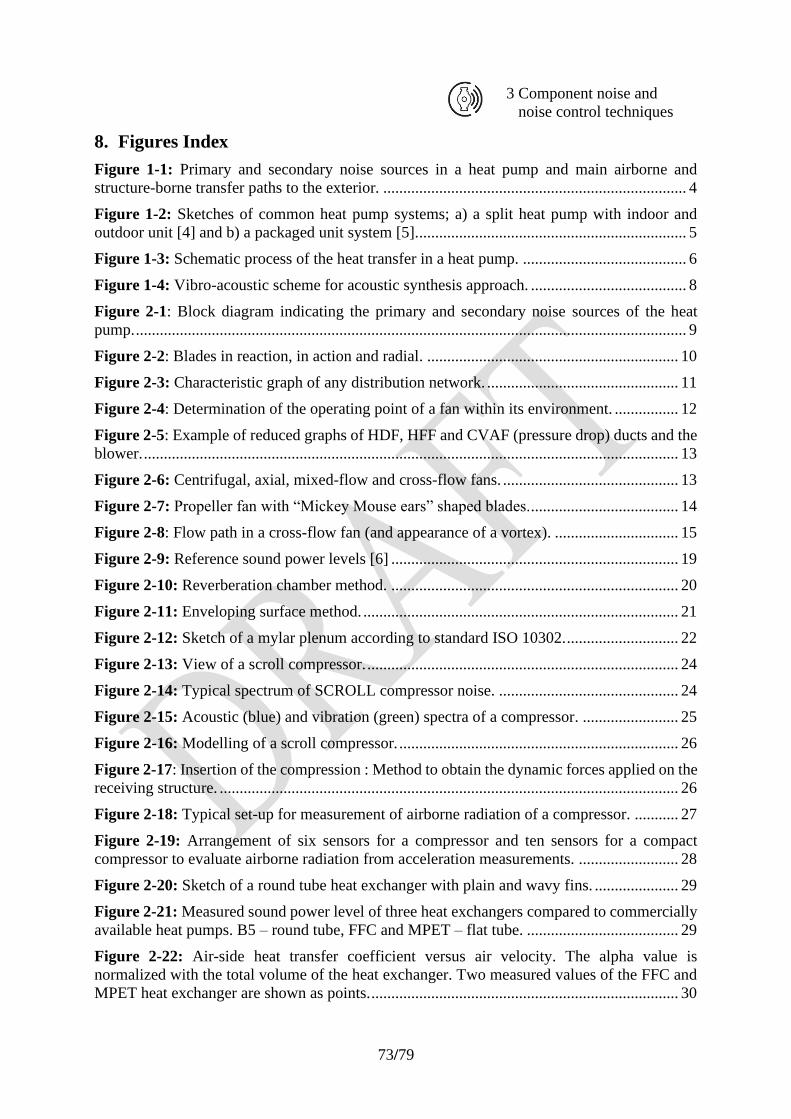
73/79



8. Figures Index

Figure 1-1: Primary and secondary noise sources in a heat pump and main airborne and

structure-borne transfer paths to the exterior. ............................................................................ 4

Figure 1-2: Sketches of common heat pump systems; a) a split heat pump with indoor and

outdoor unit [4] and b) a packaged unit system [5]. ................................................................... 5

Figure 1-3: Schematic process of the heat transfer in a heat pump. ......................................... 6

Figure 1-4: Vibro-acoustic scheme for acoustic synthesis approach. ....................................... 8

Figure 2-1: Block diagram indicating the primary and secondary noise sources of the heat

pump. .......................................................................................................................................... 9

Figure 2-2: Blades in reaction, in action and radial. ............................................................... 10

Figure 2-3: Characteristic graph of any distribution network. ................................................ 11

Figure 2-4: Determination of the operating point of a fan within its environment. ................ 12

Figure 2-5: Example of reduced graphs of HDF, HFF and CVAF (pressure drop) ducts and the

blower. ...................................................................................................................................... 13

Figure 2-6: Centrifugal, axial, mixed-flow and cross-flow fans. ............................................ 13

Figure 2-7: Propeller fan with “Mickey Mouse ears” shaped blades. ..................................... 14

Figure 2-8: Flow path in a cross-flow fan (and appearance of a vortex). ............................... 15

Figure 2-9: Reference sound power levels [6] ........................................................................ 19

Figure 2-10: Reverberation chamber method. ........................................................................ 20

Figure 2-11: Enveloping surface method. ............................................................................... 21

Figure 2-12: Sketch of a mylar plenum according to standard ISO 10302. ............................ 22

Figure 2-13: View of a scroll compressor. .............................................................................. 24

Figure 2-14: Typical spectrum of SCROLL compressor noise. ............................................. 24

Figure 2-15: Acoustic (blue) and vibration (green) spectra of a compressor. ........................ 25

Figure 2-16: Modelling of a scroll compressor. ...................................................................... 26

Figure 2-17: Insertion of the compression : Method to obtain the dynamic forces applied on the

receiving structure. ................................................................................................................... 26

Figure 2-18: Typical set-up for measurement of airborne radiation of a compressor. ........... 27

Figure 2-19: Arrangement of six sensors for a compressor and ten sensors for a compact

compressor to evaluate airborne radiation from acceleration measurements. ......................... 28

Figure 2-20: Sketch of a round tube heat exchanger with plain and wavy fins. ..................... 29

Figure 2-21: Measured sound power level of three heat exchangers compared to commercially

available heat pumps. B5 – round tube, FFC and MPET – flat tube. ...................................... 29

Figure 2-22: Air-side heat transfer coefficient versus air velocity. The alpha value is

normalized with the total volume of the heat exchanger. Two measured values of the FFC and

MPET heat exchanger are shown as points. ............................................................................. 30

74/79



Figure 2-23: Simplified flow field in a flow domain between ................................................ 31

Figure 2-24: a) Multiport extruded tubes with serpentine flat fins; b) Microchannel heat

exchanger. ................................................................................................................................ 32

Figure 2-25: Flow field in a heat pump outdoor unit. ............................................................. 32

Figure 3-1: Methods to influence the sound emission of a noise source, e.g. heat pump or motor.

.................................................................................................................................................. 33

Figure 3-2: Typical absorber materials: a) mineral wool; b) melamine foam; c) polyurethane

foam. ......................................................................................................................................... 34

Figure 3-3: Transmission paths of the power of an incident sound wave through an absorbing

obstacle. .................................................................................................................................... 34

Figure 3-4: Standing wave apparatus [8]. ............................................................................... 35

Figure 3-5: Sound absorption depending on the thickness of the layer. ................................. 36

Figure 3-6: From porous absorber to plate resonator (porous absorber with sheet metal cover)

and the scheme of a Helmholtz resonator (casing with opening). ........................................... 36

Figure 3-7: a) cross-section of an absorber-lined channel. b) basic element of a splitter type

silencer; c) combination of basic elements of a splitter type silencer. ..................................... 37

Figure 3-8: a) Components of a splitter silencer b) application of splitter silencers in a duct.

.................................................................................................................................................. 38

Figure 3-9: Insertion loss spectra in one-third octave bands of a conventional splitter silencer

and a splitter silencer with plate resonator. .............................................................................. 38

Figure 3-10: Idealized model of sound transmission through a single leaf partition. ............. 39

Figure 3-11: Sound reduction indices for infinite partitions at subcritical frequencies [3]. ... 40

Figure 3-12: Typical sound transmission ranges of a plate-like partition of finite size [13]. . 41

Figure 3-13: Schematic drawing of the transmission of structure-borne noise from a vibrating

heat pump to the environment. ................................................................................................. 43

Figure 3-14: Coupling by connections between components Source (active) – Receiver

(passive). .................................................................................................................................. 44

Figure 3-15: Experimental set-up to determine a characterisation of a compressor for structure-

borne sound. ............................................................................................................................. 45

Figure 3-16: a) Impedance of the component for 3 directions; b) Blocked force. .................. 46

Figure 3-17: Blocked forces Fb with/without isolators. ......................................................... 46

Figure 3-18: Sketches of the four idealised vibration isolation mounting systems. ............... 47

Figure 3-19: Exemplary transmissibility of a) a simple single-stage isolation system and b) a

double-stage isolation system. .................................................................................................. 48

Figure 3-20: Exemplary inverse of the isolation effectiveness of a simple single-stage isolation

system on a flexible base structure (solid line), and the transmissibility of a corresponding

single-stage vibration isolation system reacting to an infinite impedance (dashed line). ........ 50

75/79



Figure 4-1: Block diagram indicating the primary and secondary noise sources, their

interactions and main transmission paths. ................................................................................ 52

Figure 4-2:. Reciprocating compressor used as source. .......................................................... 53

Figure 4-3: Installation of the compressor in the reverberant room. ....................................... 53

Figure 4-4: Uncoupled wood box around the compressor. ..................................................... 54

Figure 4-5: Sound power level of the compressor with wood box and without the wood box.

.................................................................................................................................................. 54

Figure 4-6: Insertion loss for wood box solutions. ................................................................. 55

Figure 4-7: Foam (left) and foam + damping layer (right). ..................................................... 55

Figure 4-8: Sound power level of compressor without foam, with foam and foam + damping

layer. ......................................................................................................................................... 56

Figure 4-9: Insertion loss for foam or foam + damping layer solutions. ................................ 56

Figure 4-10:. Outline of the impeller and volute of a centrifugal fan. .................................... 58

Figure 4-11:. Serrated blade trailing edge. .............................................................................. 58

Figure 4-12: Fan with unskewed blades (a) Fan with forward-skewed blades c) Fan with

backward-skewed blades [26]. ................................................................................................. 59

Figure 4-13: Axial fan with a diffusor on the outlet side [27]. ............................................... 60

Figure 4-14:. Air-inlet grille for axial fans (a) and radial fans (b) [28]. ................................. 60

Figure 4-15: Spectra of the sound pressure level Lp, using a fan in combination with the

FlowGrid (blue graph) and without the FlowGrid (grey graph) [28]. ........................... 60

Figure 4-16: Function demonstrator of a compact ANC system which acts on both sides of the

ventilator. .................................................................................................................................. 61

Figure 4-17: a) Rotosub® system set-up, source Noctua Webpage [35] and b) illustration of the

RotoSub® system functionality , source Rotosub AB Webpage [31] . .................................... 62

Figure 5-1: Block diagram indicating the main airborne and structure-borne emission paths of

the heat pump to the exterior. ................................................................................................... 63

Figure 5-2: Bosch Compress 7400i AW with noise diffusor at the outlet [38],[39]. .............. 64

Figure 5-3: Schematic drawing of a typical feedforward ANC unit with reference and error

microphone sensors and digital control unit. ........................................................................... 65

Figure 5-4: a) 3D model of an ASC b)sound absorption coefficient (normal incidence angle)

of a porous absorber and an ASC with an open and closed control loop [40]. ........................ 65

Figure 5-5: Schematic drawing of a typical feedback ANC unit. ........................................... 66

Figure 5-6: a) and b) Retrofit Solution, Kellner Engineering GmbH, Austria; b) and c) Retrofit

Solution, Schallbox dB(A) GmbH, Germany. ......................................................................... 67

Figure 7-1: Simple web based calculation tools. .................................................................... 70

Figure 7-2:: Two-dimensional visualization of sound pressure levels. ................................... 71

Figure 7-3: Augmented reality and acoustic app. ................................................................... 71

76/79



Figure 7-4: Sound field emission studies with multiple heat pump. ....................................... 72

Figure 7-5: Analysis of unit placement, indoor & outdoor sound propagation ...................... 72

77/79



9. References

1. (2018) ENERGY ATLAS Facts and figures about renewables in Europe

2. Stefan Sobotta Praxis Wärmepumpe Technik, Planung, Installation 2018

3. Fahy FJ, Walker JG (eds) (1998) Fundamentals of noise and vibration. E & FN Spon,

London

4. Heat Pump Heating. https://www.pipeworksservices.com/heating/heating-systems/heat-

pump-heating.html. Accessed 06 May 2020

5. Vorteile Innenaufstellung Luft/Wasser-Wärmepumpe - P. Rieß GmbH. http://www.p-

riess.at/alpha-innotec/vorteile-innenaufstellung-luftwasser-waermepumpe/. Accessed 27

Aug 2019

6. Graham J. Barrie The status of fan noise measurement in North America. Fan

Noise: 293–300

7. J. Zhou, Z. Yan, Q. Gao (2017) Development-and-Application-of-Microchannel-Heat-

Exchanger-for-Heat-Pump

8. Daniel A. Russel Absorption Coefficients and Impedance

9. Möser M (2007) Technische Akustik, 7., erweiterte und aktualisierte Auflage. VDI-

Buch. Springer-Verlag Berlin Heidelberg, Berlin, Heidelberg

10. Piening W (1937) Schalldämpfung der Ansauge- und Auspuffgeräusche von

Dieselanlagen auf Schiffen. Zeitschrift des Vereines Deutscher Ingenieure 81: 770–776

11. DIN EN ISO 7235:2010-01, Akustik_- Labormessungen an Schalldämpfern in Kanälen_-

Einfügungsdämpfung, Strömungsgeräusch und Gesamtdruckverlust (ISO_7235:2003);

Deutsche Fassung EN_ISO_7235:2009

12. Fahy F, Gardonio P (2007) Sound and structural vibration: Radiation, transmission and

response, 2. ed. ScienceDirect. Elsevier Acad. Press, Amsterdam

13. Fasold W, Veres E (1998) Schallschutz und Raumakustik in der Praxis:

Planungsbeispiele und konstruktive Lösungen, 1. Aufl. Verl. für Bauwesen, Berlin

14. Schirmer W (2006) Technischer Lärmschutz: Grundlagen und praktische Maßnahmen

zum Schutz vor Lärm und Schwingungen von Maschinen ; mit 40 Tabellen, 2., bearb.

und erw. Aufl. VDI-Buch. Springer, Berlin

15. Nelson PA, Elliott SJ (1992) Active control of sound. Acad. Press, London

16. C.H. Hansen SDS Active Control of Noise and Vibration

17. Gardonio P, Rohlfing J (2014) Modular feed-forward active noise control units for

ventilation ducts. J Acoust Soc Am 136: 3051. https://doi.org/10.1121/1.4900571

18. Elliott SJ (2005) Signal processing for active control, Transferred to digital printing

2005. Signal processing and its applications. Academic Press, San Diego, Calif.

19. Kuo S-M, Morgan DR (1996) Active noise control systems: Algorithms and DSP

implementations. A Wiley-Interscience publication. Wiley, New York, NY

20. Leistner P, Krueger J., Leistner M. (1996) Hybride Schalldämpfer - Hohe Dämpfung bei

tiefen Frequenzen

78/79



21. Fahy F, Walker J (2004) Advanced Applications in Acoustics, Noise and Vibration. Spon

Press, London

22. Fuller CR, Nelson PA, Elliott SJ (1996) Active control of vibration. Academic Press,

London, San Diego

23. Gladwell GML, Preumont A (2011) Vibration Control of Active Structures, vol 179.

Springer Netherlands, Dordrecht

24. Bös J, Janssen E, Kauba M et al. (2008) Active vibration reduction applied to the

compressor of an air‐conditioning unit for trams. J Acoust Soc Am: 5503–5506.

https://doi.org/10.1121/1.2935763

25. Thomas Carolus-Ventilatoren Aerodynamischer Entwurf Schallvorhersage

26. Felix Czwielong, Florian Krömer, Stefan Becker Experimental investigations of the

sound emissons of axial fans under the influence of suction-side heat exchangers

27. (2020) AxiTop - Diffusor für Axialventilatoren.

https://www.ebmpapst.com/de/products/axial-fans/diffusor/axitop.html. Accessed 19

May 2020

28. EBM_Papst_Vorleitgitter_FlowGrid_DE

29. Marc SCHNEIDER RB (2012) Implementation of an active noise control into different

fan applications

30. (2020) Silentium – Active noise reduction, control and cancellation solutions.

https://www.silentium.com/. Accessed 03 Sep 2020

31. (2020) RotoSub AB. http://www.rotosub.com/. Accessed 03 Sep 2020

32. L. Stromback MO (2013) RotoSub – The self silencing fan technology

33. Lars Stromback (2007) Acoustic Element(US20070230720 A1)

34. Lars Stromback (2010) Acoustic Element(EP1752016 B1)

35. (2020) Noctua.at - Premium cooling components designed in Austria. https://noctua.at/.

Accessed 04 Sep 2020

36. (2020) Asia Vital Components. http://www.avc.co/en-us/. Accessed 04 Sep 2020

37. Asia Vital Components Co., Ltd (2015) FAN ACTIVE NOISE SELF-LOWERING

SYSTEM(US20150296295A1)

38. Compress 7400i AW | Luft-Wasser Wärmepumpen | Wärmepumpen | Produkte |

Wohngebäude. https://www.bosch-

thermotechnology.com/de/de/ocs/wohngebaeude/compress-7400i-aw-1150650-p/.

Accessed 19 May 2020

39. Bosch (2020) Compress 7400i AW | Luft-Wasser Wärmepumpen | Bosch.

https://www.bosch-thermotechnology.com/de/de/ocs/wohngebaeude/compress-7400i-

aw-1150650-p/. Accessed 23 Sep 2020

40. Jens Rohlfing, Karlheinz Bay, Peter (2019) Design and applications of lean active

resonator silencer cassettes

41. Jan Krüger (1999) Berechnung und praktischer Einsatz aktiv absorbierender

Schalldämpfer

79/79



42. Kellner Engineering GmbH. https://www.kellner-engineering.com/. Accessed 27 Aug

2019

43. SchallBox - Ihr Partner für effektiven Schallschutz. https://www.schallbox.de/. Accessed

27 Aug 2019

44. Elliott SJ (2008) A review of active noise and vibration control in road vehicles. 981.

University of Southampton

45. H. Sano, T. Yamashita, M. Nakamura (2002) Recent application of active noise and

vibration to automobiles 2002

46. Daley S, Hätönen J, Owens DH (2005) ACTIVE VIBRATION ISOLATION IN A

“SMART SPRING” MOUNT1 USING A REPETITIVE CONTROL APPROACH.

IFAC Proceedings Volumes 38: 55–60. https://doi.org/10.3182/20050703-6-CZ-

1902.01951

Overview on Heat Pump Component Noise and Noise Control ...

Documents