Overreaction evidence from large-cap stocks

Overreaction Evidence from Large-Cap Stocks

*Tibebe A. Assefa School of Business

Bradford Hall Room # 134 400 East Main Street, Frankfort, KY 40601

Kentucky State University Telephone: 502 597 6912

Email: [email protected]

Omar A. Esqueda Assistant Professor of Finance

Department of Accounting, Finance, & Economics Tarleton State University

1333 W. Washington, Stephenville, TX 76402 Email: [email protected]

Emilios C. Galariotis

Professor of Finance, Director of the Centre for Financial and Risk Management Department of Finance,

Audencia Nantes School of Management, PRES-LUNAM 8 Route De La Joneliere, 44300 Nantes, France

Email: [email protected]

To appear in: Review of Accounting and Finance, 2014

Overreaction Evidence from Large-Cap Stocks Abstract Purpose – The purpose of this paper is to assess the performance of a contrarian investment strategy focusing on frequently traded large-cap U.S. stocks. We address previous criticisms that losers’ gains are not due to overreaction but due to their tendency to be thinly traded and smaller-sized firms than winners. Design/Methodology/Approach – We construct portfolios based on past performance and examine whether contrarian returns exist. We employ the Capital Asset Pricing Model (CAPM), Fama and French three-factor model and the Carhart’s (1996) momentum portfolio to test whether excess returns are feasible in a contrarian strategy. Findings – The results show an asymmetric performance following portfolio formation. Whereas both, winners and losers portfolios, have gains during holding periods, losers outperform winners at all times, and with a differential of up to 29.2% thirty-six months after portfolio formation. Furthermore, the loser and the winner portfolios’ alphas are significant, suggesting that the CAPM and the multifactor models are unable to explain return differentials between winners and losers. Our evidence supports two main conclusions. First, stock market overreaction still holds for a sample of large firms. Second, this is robust to the Fama and French (1993, 1996) three-factor model and Carhart (1997) momentum portfolio. Our findings emphasize the relevance of a contrarian strategy when rebalancing investment portfolios. Practical Implications – Portfolio managers can improve stock returns by selling past winners and buying previous loser large-cap U.S. stocks.

Originality/Value – This paper is the first, to the authors' knowledge, to examine frequently traded large-cap U.S. stocks in order to avoid infrequent trading and size concerns.

JEL classification: G11, G12, G14 Keywords: Overreaction, CAPM, Stock Market Anomaly, Three-factor model Paper Type: Research Paper

2

I. Introduction

A plethora of papers has been devoted to testing the overreaction hypothesis following its

inception by De Bondt and Thaler (1985). According to the overreaction hypothesis, stocks that

have performed badly in the past, will exhibit superior performance in the future and vice versa.

Hence, a contrarian portfolio that takes long positions in past losers and short positions in past

winners should provide positive above normal returns as a result of the return reversals. This

phenomenon pauses one of the most serious violations to the efficient market hypothesis in the

literature according to Dimson and Mussavian (2000). Overreaction, as the name suggest, is

ascribed to behavioral characteristics that affect decision making and reaction under uncertainty,

for example Malkiel (2003, p. 80) suggests that “Undoubtedly, some market participants are

demonstrably less than rational. As a result, pricing irregularities and even predictable patterns in

stock returns can appear over time and even persist for short periods. Moreover, the market cannot

be perfectly efficient, or there would be no incentive for professionals to uncover the information

that gets so quickly reflected in market prices.”

On the whole, the evidence has supported the overreaction hypothesis (see Howe, 1986;

Porterba and Summers, 1988; Chopra et al., 1992; and Kassimatis et al., 2008). This however has

not precluded alternative propositions. Most notably, Conrad and Kaul (1993) put forward the bid-

ask bounce and infrequent trading as potential explanations for return reversals. Zarowin (1990)

attributes them to the size effect and not overreaction1. Most recently, Clements et al. (2009)

suggest that overreaction is seemingly driven by firm size and value.

The main purpose of this paper is to contribute to the above literature by investigating the

overreaction hypothesis while controlling for size, value and momentum effects. This paper

1 Antoniou et al. (2005, 2006) also show that the magnitude of the contrarian profits is substantially affected by firm size in a sample of emerging and developed country firms.

3

contributes to the existing literature in that unlike previous studies that examine the size effect, we

focus on large market capitalization firms (i.e. 5 billion USD and higher) that trade in the U.S.

stock market (i.e. NYSE, Amex, and NASDAQ). Our choice offers a clean and direct method to

deal with the proposition that losers outperform not due to investor overreaction, but due to their

tendency to be smaller sized firms than winners (Zarowin, 1990; Ball et al., 1995). If the

phenomenon is inversely related to size, then, the largest stocks in our sample should not

experience any abnormal overreaction performance. This sample has the added benefit that it

consists of the most frequently traded stocks in the U.S., hence, it controls in a simple uncontested

and non-model- related way for the effect of the bid-ask spread due to infrequent trading.

The paper also offers recent out-of-sample evidence on overreaction given the arguments

of Dimson and Mussavian (2000) that whether such reversal patterns really exist is “a matter of

controversy” as they appear not to be so robust over time. Roll (1994) argues that they may be

chance events, hence more research is needed, and the paper contributes towards this.

Our findings suggest that after controlling for the abovementioned explanations, there are

significant profits to be made by contrarians due to winner and loser stock overreactions. These

reactions are asymmetric consistent with De Bondt and Thaler (1985), Pettengill and Jordan (1990)

and others. More specifically, losers revert to winners, but winners do not exhibit losses but

continue to deliver positive returns that however are lower than in the past, consistent with earlier

evidence by Pettengill and Jordan (1990). This can be partially explained by investor overreaction

to recent good (bad) news: those that gained above the market will revert to their natural level and

those that lost will regain their losses. Therefore, consistent with the overreaction hypothesis,

investors put more weight on recent information than they do on historical ones. Two other factors

may also be at related to the above result: large-cap firms are less volatile than small-cap ones and

4

that may inhibit the reversals in tandem with the sample period (1976 to 2008) that is a relatively

high growth stock market period and could lead to gains for both losers and winners.2 This can be

particularly relevant to winners that have been shown to have higher betas (De Bondt and Thaler,

1987) hence they would benefit the most during a growing market period not experiencing losses.

Yet, if the theory is correct they should gain by less than in the past and less than past losers even

in such periods. The evidence shows that despite the asymmetry in the reaction, former losers

deliver holding period returns that are 29.2 percent more than the past winners do.

Fama and French (1993) showed that the traditional capital asset pricing model (CAPM)

is not sufficient in explaining the cross section of returns and unearthed a strong cross-sectional

relationship between returns, firm size, and value characteristics. The exact nature of this

relationship is still debated and the most compelling explanation is that these factors capture the

risk of small size and growth opportunities of the firm, or that they act as a mispricing proxy. The

paper also contributes to this literature. More specifically to explain the differential returns

between the winner and loser portfolios, we further estimate traditional and augment versions of

the CAPM for the winner and loser portfolios. In this process, we also control for factors such as

size (SMB), book to market value (HML) (Fama and French, 1996), and momentum (MOM) (

Carhart, 1997) among others.

The results from the above process indicate that losers have lower beta (β=0.99) on average

than winners (β=1.29), consistent with De Bondt and Thaler (1985), and with our earlier arguments

that it is possible that the higher returns of the winner portfolios are the result of higher risk

associated with them during a period of market growth. Furthermore, our CAPM results indicate

2 For instance, the S&P 500 grew at an annual rate of 27.3% from January 1976 to December 2008, our sample period (from 90.19 to 903.25 points), despite the major dips suffered during 2000 and 2008 in the stock market and the fact that S&P 500 index excludes dividend payments.

5

that the majority of the loser and the winner portfolios alphas are significant; this suggests that the

CAPM in conjunction with size, book-to-market, and momentum controls is not enough to explain

the return differentials between the winner and the loser portfolios. This is consistent with evidence

that the reaction to firm specific news (from the part of past losers) is responsible for return

reversals caused by overreaction; while the reaction of winners relates more to market news, i.e.

systematic risk, yet with a small contribution to contrarian performance (Jegadeesh and Titman,

1995; Antoniou et al., 2005). Thus, the difference in returns between the winners and losers not

captured by all the above considerations and controls could be explained by the overreaction

hypothesis.

Overall, our findings indicate that even though the version of the CAPM used can partially

account for the return differentials between winners and losers, there is still large and unexplained

(firm-specific) variation between the two portfolios. This finding provides strong evidence in favor

of the overreaction hypothesis, as the model (Fama and French, 1996) that is supposed to explain

the phenomenon does not do so even for very large transparent and liquid securities. This finding

is in line with evidence from other markets such as the UK, Greece, etc. (Antoniou et al. 2005,

2006). In summary our result suggests that, first; there is overreaction in the U.S. stock market for

a more recent period. Second, the overreaction hypothesis holds even after controlling for size,

book-to-market value and momentum.

The remainder of this paper is structured as follows: the next section briefly reviews the

relevant literature; the third section, presents the data, descriptive statistics and the methodology

employed. The fourth section presents and discusses the empirical results, and the last section

concludes the paper.

6

II. Literature Review

The first paper to address the overreaction hypothesis is by De Bondt and Thaler (1985)

and is entitled “Does the Stock Market Overreact?” Using CRSP monthly return data, they find

substantial market inefficiencies of the weak form. Consistent with the predictions of the

overreaction hypothesis, portfolios of prior “losers” are found to outperform prior “winners.”

Thirty six months after portfolio formation, the losing stocks have earned about 25% more than

the winners, even though the latter are significantly more risky.

On a follow up paper, De Bondt and Thaler (1987) report additional evidence in support

of the overreaction hypothesis. Their principal findings are: first, excess returns in the holding

period (and particularly during the month of January) are negatively related to long-term formation

period performances for both winners and losers. For winners, January excess returns are

negatively related to the excess returns for the prior December, possibly reflecting a capital gains

tax “lock-in” effect. Second, the winner-loser effect cannot be attributed to changes in risk as

measured by the CAPM slope coefficients. Third, the winner-loser effect is not primarily a size

effect, a finding that Zarowin (1990) will contest. Fourth, the small firm effect is partly a losing

effect, but even if the losing firm effect is removed, there are still excess returns to small firms.

Clare and Thomas (1995), using UK data from 1955 to 1990 drawn from a random sample

of up to 1000 stocks in any one year, find similar result with De Bondt and Thaler. That is, losers

outperform previous winners over a two year period by statistically significant 1.7% per annum.

They also find the losers tend to be small, and that the limited overreaction effect documented is

probably due to the small firm effect. Which is something that Antoniou et al. (2006) contest,

adding to the uncertainty regarding the role of the size effect. Dissanaike (1997) also investigates

7

the overreaction hypothesis for the UK stock market. His finding is in favor of the overreaction

hypothesis, while he also finds evidence of asymmetric reactions for winners and losers and

supports the U.S. findings of De Bondt and Thaler (1985) that losers are less risky than winners.

Fama and French (1988) examine autocorrelations of stock returns for increasing holding

periods. In their results for the 1926 to 1985 time window, they discover large negative

autocorrelations for return horizons that expand beyond a year consistent with the hypothesis that

mean-reverting price components are important in the variation of returns. Their results add

evidence to the statement that stock returns are predictable, and more importantly that they are in

the direction suggested by the overreaction hypothesis consistent with long term return reversals.

The above result is consistent with the momentum effect related to an underreaction

phenomenon, where past winners tend to outperform past losing stocks (Jegadeesh and Titman,

1993). This is not inconsistent with overreaction hypothesis, given that over- and underreaction

are experienced at different horizons. Overreaction is a long term effect (De Bondt and Thaler,

1985), whereas, underreactionis a short-term phenomenon (Jegadeesh and Titman 1995, Antoniou

et al. 2005). Underreaction is found for periods of 1, 3 to 12 months (Jegadeesh and Titman, 1993).

Carhart (1997) also confirms this result using a sample of mutual funds. Extant literature supports

the proposition that both phenomena are connected and that overreaction is the result of a

prolonged underreaction. For example Barberis, Shleifer, and Vishny (1997) observe short-run

underreaction and longer-run overreaction is consistent with their psychological model. Amir and

Ganzach (1998) find that both overreaction and underreaction are present, but that each relates to

different kind of information. Given the above results, it is interesting to consider a momentum

variable in addition to the factors that affect the cross section of returns. Our paper uses the Carhart

(1997) momentum portfolio to address this concern. More recently, Pyo and Shin (2013) find that

8

momentum provides excess return not contrarian strategy for the Korean stock market. Leivo

(2012) find that in bullish market momentum adds positive value to investors while in the bearish

market momentum adds negative value to investor in the Finnish stock market. On the other hand,

Youssef et al. (2010) reported that in the recent U.S. market momentum is no more profitable.

The evidence, however, is far from conclusive and a number of questions remain open in

the literature. For example the issue of the size effect has received contradictory results, is still

debated starting from Ball et al. (1995) and Zarowin (1990) who show that the tendency for losers

to outperform winners is not due to investor overreaction, but because they are smaller-sized firms

than winners. More specifically, it is supported that when losers are compared to winners of equal

size, there is little evidence of any return discrepancy, and in periods when winners are smaller

than losers, winners outperform losers. Thus, the winner vs. loser phenomenon found by De Bondt

and Thaler (1985) appears to be another manifestation of the size effect in finance. This finding

motivates the sample selection for this study. We focus on large size firms during a recent sample

period, testing for the presence of abnormal returns linked to reversals in stock performance.

Using CRSP data for the period between 1926 and 2003, Clements et al. (2009), provide

preliminary support for De Bondt and Thaler’s (1985) findings; reporting that the overreaction

anomaly has not only persisted over the past many years but also has increased when risk is not

controlled. However, using the three-factor model of Fama and French (1993, 1996), they find no

statistically significant alphas (a necessary condition to support the overreaction anomaly in the

form of abnormal performance beyond risk). As a matter of fact, their evidence suggests that

contrarian return is driven by factors such as size and value, but not by investors’ behavioral biases.

We propose that given the Antoniou et al.’s (2006), findings on the U.K., we must investigate the

9

above issue using a different sample to test the sensitivity of the arguments to different

methodological approaches.

III. Data and Methodology

This study uses CRSP monthly data for the period of January 1976 to December 2008. The

sample includes only stocks that have a market capitalization of five billion U.S. dollar or more

i.e. large market capitalization stocks. According to CRSP, there are currently 626 stocks that

satisfy this condition in the U.S stock market.

Each portfolio of winner (loser) stocks is constructed based on the top (bottom) decile

ranking of abnormal returns in the previous three-year period. Hence, in each of the ten periods

we have two portfolios, one with winners and one with losers. Table 1 presents the number of

stocks included in each of the ten, three-year period portfolios, and provides the average excess

returns of both winner and loser portfolios for each portfolio formation period. Note that each

individual portfolio of winners or losers is, on average, comprised of forty-four stocks, therefore

we achieve a good level of diversification given the number and mix of securities in the portfolios.

The CRSP equally weighted NYSE, Amex, and NASDAQ market index is used to calculate excess

returns.

// Insert Table 1 Here//

Consistent with the aims of the study, in order to make it comparable to previous ones, the

methodology employed here is similar to that used by De Bondt and Thaler (1985), as this has

been followed by the extant literature in long-term studies. In general, we use monthly cumulative

excess returns, where the excess return of stock j at time t (Ejt) is given as Ejt = Rjt - Rmt, where Rjt

is the return of stock j at time t, and Rmt is return of the CRSP NYSE/Amex/Nasdaq equal-weighted

market index at time t. Our starting point is the 626 stocks we selected using the required market

10

capitalization for our study. As our initial list is current, when we go back to the 1970’s less and

less of them meet the criteria and have data at CRSP, and as we get closer to current date, more

and more of them meet the criteria and have data. This pattern is clearly depicted in Table 1. For

the portfolio formation period, we use the excess returns for a period of 36 months. At each of ten

portfolio formation dates (December 1978, December 1981, …, Dec. 2005) the excess cumulative

returns are ranked from low to high and loser and winner portfolios are formed accordingly.3

The winner and loser portfolio performances are followed for the next 36 months (the test

or holding period), and cumulative excess returns are calculated for each of the ten independent

portfolios. We test the difference in average cumulative excess returns of winner and loser

portfolios. Using the Excess Cumulative Returns (ECR) from all 10 test periods, the average

ECR’s are calculated for both portfolios and each month between t=1 and t=36. They are denoted

AECRW,t and AECRL,t . The Overreaction hypothesis predicts that, for t>0 AECRW,t <0 and

AECRL,t >0, that implies (AECRL,t - AECRW,t ) >0. However, as long as the latter inequality holds,

the evidence can be broadly consistent with the overreaction hypothesis, as past winners can

experience holding period losses compared to, their formation period performance and to, past

loser holding period performance, but their returns may not be necessarily negative.

Furthermore, as explained earlier, we test whether the difference in excess returns of the

loser and the winner portfolios are explained by a simple CAPM and a modified CAPM that

controls for size and standard deviation of the cumulative excess returns for each of the portfolios

in our study. The Models are:

Rit - Rft =α + β(Rmt - Rft) + εt (1)

3 We remind the reader that the number of firms that are assigned to the winner and loser portfolios in each formation period is available in Table 1.

11

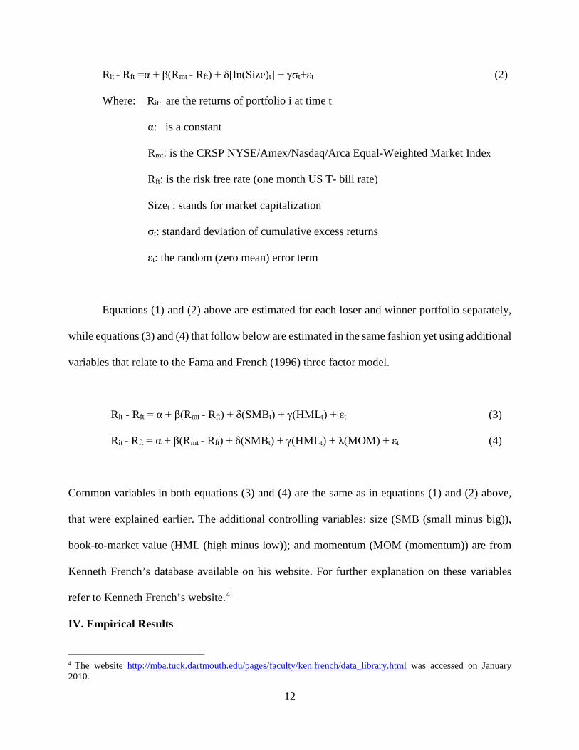
Rit - Rft =α + β(Rmt - Rft) + δ[ln(Size)t] + γσt+εt (2)

Where: Rit: are the returns of portfolio i at time t

α: is a constant

Rmt: is the CRSP NYSE/Amex/Nasdaq/Arca Equal-Weighted Market Index

Rft: is the risk free rate (one month US T- bill rate)

Sizet : stands for market capitalization

σt: standard deviation of cumulative excess returns

εt: the random (zero mean) error term

Equations (1) and (2) above are estimated for each loser and winner portfolio separately,

while equations (3) and (4) that follow below are estimated in the same fashion yet using additional

variables that relate to the Fama and French (1996) three factor model.

Rit - Rft = α + β(Rmt - Rft) + δ(SMBt) + γ(HMLt) + εt (3)

Rit - Rft = α + β(Rmt - Rft) + δ(SMBt) + γ(HMLt) + λ(MOM) + εt (4)

Common variables in both equations (3) and (4) are the same as in equations (1) and (2) above,

that were explained earlier. The additional controlling variables: size (SMB (small minus big)),

book-to-market value (HML (high minus low)); and momentum (MOM (momentum)) are from

Kenneth French’s database available on his website. For further explanation on these variables

refer to Kenneth French’s website.4

IV. Empirical Results

4 The website http://mba.tuck.dartmouth.edu/pages/faculty/ken.french/data_library.html was accessed on January 2010.

12

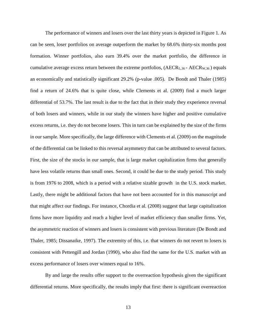
The performance of winners and losers over the last thirty years is depicted in Figure 1. As

can be seen, loser portfolios on average outperform the market by 68.6% thirty-six months post

formation. Winner portfolios, also earn 39.4% over the market portfolio, the difference in

cumulative average excess return between the extreme portfolios, (AECRL,36 - AECRW,36 ) equals

an economically and statistically significant 29.2% (p-value .005). De Bondt and Thaler (1985)

find a return of 24.6% that is quite close, while Clements et al. (2009) find a much larger

differential of 53.7%. The last result is due to the fact that in their study they experience reversal

of both losers and winners, while in our study the winners have higher and positive cumulative

excess returns, i.e. they do not become losers. This in turn can be explained by the size of the firms

in our sample. More specifically, the large difference with Clements et al. (2009) on the magnitude

of the differential can be linked to this reversal asymmetry that can be attributed to several factors.

First, the size of the stocks in our sample, that is large market capitalization firms that generally

have less volatile returns than small ones. Second, it could be due to the study period. This study

is from 1976 to 2008, which is a period with a relative sizable growth in the U.S. stock market.

Lastly, there might be additional factors that have not been accounted for in this manuscript and

that might affect our findings. For instance, Chordia et al. (2008) suggest that large capitalization

firms have more liquidity and reach a higher level of market efficiency than smaller firms. Yet,

the asymmetric reaction of winners and losers is consistent with previous literature (De Bondt and

Thaler, 1985; Dissanaike, 1997). The extremity of this, i.e. that winners do not revert to losers is

consistent with Pettengill and Jordan (1990), who also find the same for the U.S. market with an

excess performance of losers over winners equal to 16%.

By and large the results offer support to the overreaction hypothesis given the significant

differential returns. More specifically, the results imply that first: there is significant overreaction

13

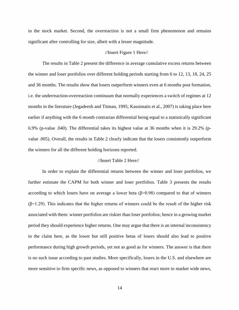
in the stock market. Second, the overreaction is not a small firm phenomenon and remains

significant after controlling for size, albeit with a lesser magnitude.

//Insert Figure 1 Here//

The results in Table 2 present the difference in average cumulative excess returns between

the winner and loser portfolios over different holding periods starting from 6 to 12, 13, 18, 24, 25

and 36 months. The results show that losers outperform winners even at 6 months post formation,

i.e. the underreaction-overreaction continuum that normally experiences a switch of regimes at 12

months in the literature (Jegadeesh and Titman, 1995; Kassimatis et al., 2007) is taking place here

earlier if anything with the 6 month contrarian differential being equal to a statistically significant

6.9% (p-value .040). The differential takes its highest value at 36 months when it is 29.2% (p-

value .005). Overall, the results in Table 2 clearly indicate that the losers consistently outperform

the winners for all the different holding horizons reported.

//Insert Table 2 Here//

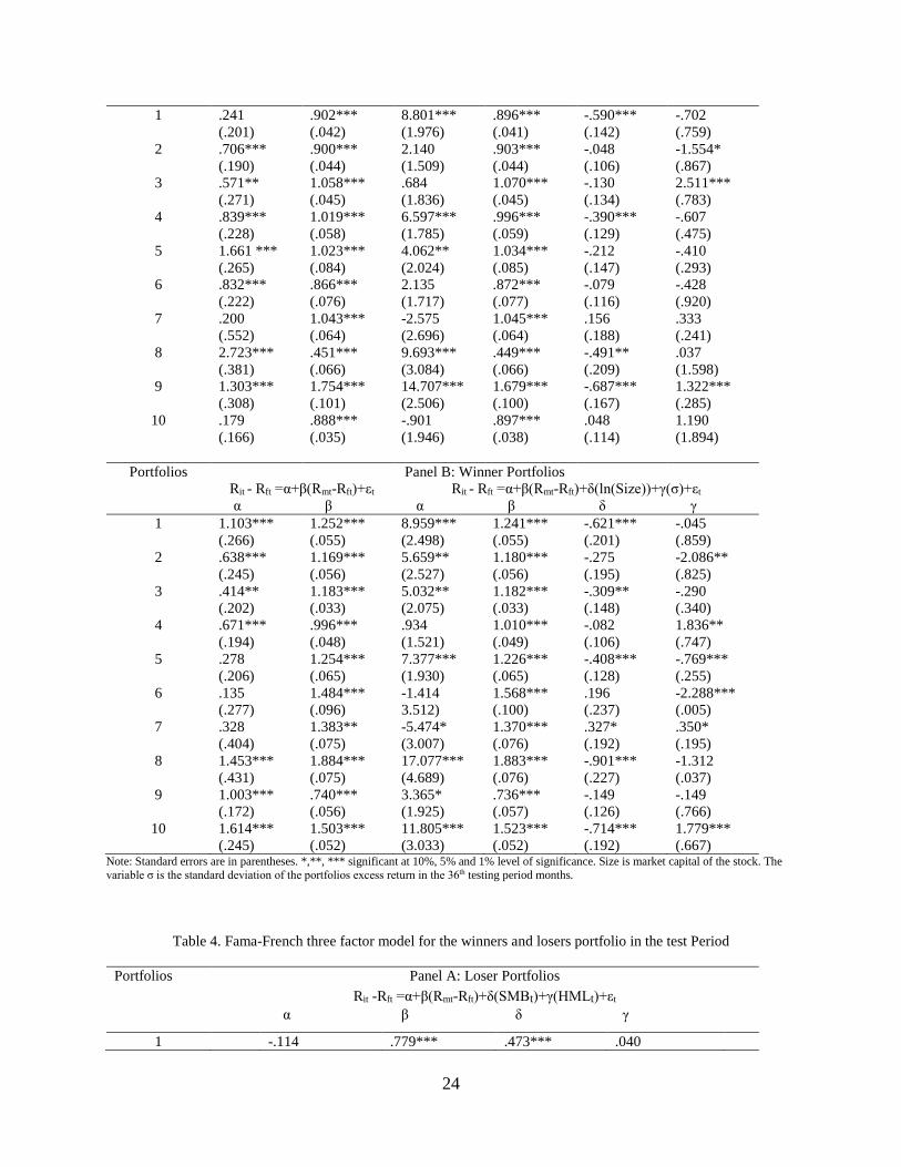
In order to explain the differential returns between the winner and loser portfolios, we

further estimate the CAPM for both winner and loser portfolios. Table 3 presents the results

according to which losers have on average a lower beta (β=0.98) compared to that of winners

(β=1.29). This indicates that the higher returns of winners could be the result of the higher risk

associated with them: winner portfolios are riskier than loser portfolios; hence in a growing market

period they should experience higher returns. One may argue that there is an internal inconsistency

in the claim here, as the lower but still positive betas of losers should also lead to positive

performance during high growth periods, yet not as good as for winners. The answer is that there

is no such issue according to past studies. More specifically, losers in the U.S. and elsewhere are

more sensitive to firm specific news, as opposed to winners that react more to market wide news,

14

i.e. systematic risk (Jegadeesh and Titman, 1995; Antoniou et al., 2005, 2006). Hence, the overall

performance of losers is defined by firm-specific news as well as betas.

Furthermore, Table 3 shows that both loser and winner portfolios alphas are significant.

For example, for the loser portfolio the highest alpha value for the traditional (augmented) CAPM

specification is a statistically significant 2.723 (14.707). For the winner portfolio the alphas of the

traditional (augmented) CAPM specification are 1.614 (17.077). Both of the above sets of results

are consistent with the earlier discussion that there is a larger unexplained component of returns

for losers that relates to firm specific information. The alphas suggest that the CAPM alone is not

enough to explain the return differentials between the winner and the loser portfolios. The

unexplained variation could be explained by the overreaction hypothesis.

The results of Table 3 also indicate that size is negatively associated with both winner and

loser portfolios, and is significant for almost half of the portfolios. This simply means that the

returns are lower for larger firms, but this holds for both winners and losers cancelling out any size

effect. Similarly standard deviation alone cannot explain the difference in their returns between

the losers and the winners as here the signs are also mixed unlike the size factor coefficients. One

issue that clearly comes out, however, is that these factors cannot rationalize the return differential

between the two extreme performance portfolios; their effect is more prominent on losers, since

half of the loser portfolios deliver insignificant returns once these factors are considered. In other

words, losers are more affected by company size and volatility of returns compared to winners.

//Insert Table 3 Here//

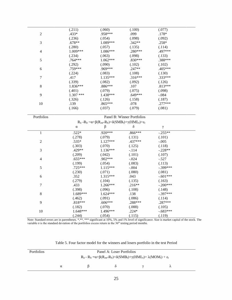
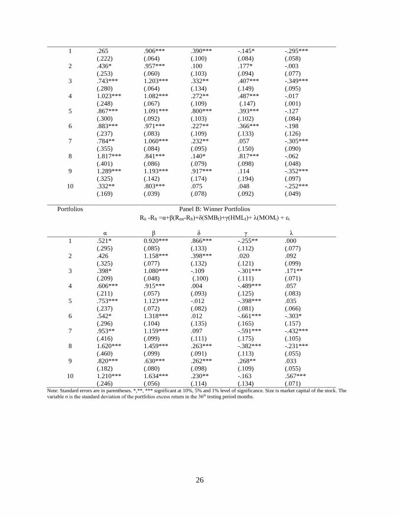
Tables 4 and 5 present the results of estimating equations (3) and (4) respectively, as

presented in the methodology section. In both tables, winner and loser portfolios are sensitive to

the (SMB) and (HML) factors, that is, they are sensitive irrespective of whether the Carhart (1997)

15

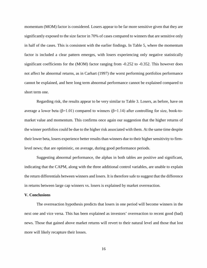
momentum (MOM) factor is considered. Losers appear to be far more sensitive given that they are

significantly exposed to the size factor in 70% of cases compared to winners that are sensitive only

in half of the cases. This is consistent with the earlier findings. In Table 5, where the momentum

factor is included a clear pattern emerges, with losers experiencing only negative statistically

significant coefficients for the (MOM) factor ranging from -0.252 to -0.352. This however does

not affect he abnormal returns, as in Carhart (1997) the worst performing portfolios performance

cannot be explained, and here long term abnormal performance cannot be explained compared to

short term one.

Regarding risk, the results appear to be very similar to Table 3. Losers, as before, have on

average a lower beta (β=1.01) compared to winners (β=1.14) after controlling for size, book-to-

market value and momentum. This confirms once again our suggestion that the higher returns of

the winner portfolios could be due to the higher risk associated with them. At the same time despite

their lower beta, losers experience better results than winners due to their higher sensitivity to firm-

level news; that are optimistic, on average, during good performance periods.

Suggesting abnormal performance, the alphas in both tables are positive and significant,

indicating that the CAPM, along with the three additional control variables, are unable to explain

the return differentials between winners and losers. It is therefore safe to suggest that the difference

in returns between large cap winners vs. losers is explained by market overreaction.

V. Conclusions

The overreaction hypothesis predicts that losers in one period will become winners in the

next one and vice versa. This has been explained as investors’ overreaction to recent good (bad)

news. Those that gained above market returns will revert to their natural level and those that lost

more will likely recapture their losses.

16

This paper tests the overreaction hypothesis for the U.S. market from 1976 to 2008 for

large stocks with market capitalization of at least five billion U.S. dollars. We find that:

• Although both the losers and the winners gain in the future, the losers gain 29.2% above

winners, consistent with the overreaction hypothesis. Clements et al. (2009) find a much

larger differential of 53.7%, while De Bondt and Thaler (1985) find a differential of 24.6%.

Our lower differential compared to of Clements et al. (2009) could be due to the fact that

our sample includes only large cap firms .

• Winners have more systematic risk than losers. This can explain the first bullet point, i.e.

why winners do not revert (due to positive betas) and why losers do so (if one considers

that losers are more sensitive to firm specific news, it is easy to explain why they win by

much more than winners do during an expansionary period even though they have a lower

beta).

• Even though CAPM (traditional and augmented with other factors) explains partially the

difference in returns between losers and winners, we still garner statistically and

economically significant alphas in both portfolios.

Overall, the results show that: first overreaction in the stock market still exists in recent

times. When thinly-traded and small-sized firms are omitted from the sample we still find evidence

that losers gain more than winners and alphas are significant when size, SMB, HML, firm specific

risk, and MOM are included. Our evidence supports the idea that investors can take advantage of

market inefficiencies and earn abnormal returns by following a contrarian strategy in portfolios of

large market capitalization stocks. The main implication of this manuscript is that portfolio

managers can improve stock returns by selling winner and buying loser large-cap stocks in the

U.S. stock markets.

17

REFERENCES

Amir, E. and Ganzach, Y. (1998), “Overreaction and underreaction in analysts’ forecasts”, Journal of Economic Behaviour & Organisation, Vol. 37, pp. 333-347.

Antoniou, A., Galariotis, E. C., and Spyrou, S. I. (2005), “Contrarian profits and the overreaction

hypothesis: the case of the Athens stock exchange”, European Financial Management, Vol. 11, pp. 71-98.

Antoniou, A., Galariotis, E. C., and Spyrou, S. I. (2006), “Short-term contrarian strategies in the

London Stock Exchange: are they profitable? Which factors affect them?”, Journal of Business Finance & Accounting, Vol. 33, pp. 839-867.

Ball, R., Kothari, S. P. and Shanken, J. (1995), “Problems in measuring portfolio performance: an

application to contrarian investment strategies”, Journal of financial Economics, Vol. 38, pp.79-107.

Barberis, N., Shleifer, A., and Vishny R. (1998), “A model of investor sentiment”, Journal of

Financial Economics, Vol. 49, pp. 307-343. Chan, K.C. (1988). “On the Contrarian Investment Strategy”, Journal of Business, Vol. 61, pp.

147-163 Conrad, J., and Kaul, G. (1993), “Long-term Market overreaction or biases in computed returns?”,

The Journal of Finance, Vol. 48, pp. 39-63. Carhart, M. (1997), “On Persistence in Mutual Fund Performance”, The Journal of Finance, Vol.

52, pp. 57-82. Chopra, N., Lakonishok, J. and Ritter, J.R. (1992), “Measuring abnormal performance: do stocks

overreact?”, Journal of Financial Economics, Vol. 31, pp. 235-268. Chordia, T., Roll, R., & Subrahmanyam, A. (2008). Liquidity and market efficiency. Journal of

Financial Economics, 87(2), 249-268. Clare, A. and Thomas, S. (1995), “The overreaction hypothesis and the UK stock market”, Journal

of Business Finance & Accounting, Vol. 22, pp. 961- 973. Clements, A., Drew, M.E., Reedman, E.M. and Veeraraghavan, M. (2009), “The death of the

overreaction anomaly? A multifactor explanation of the contrarian returns”, Investment Management and Financial Innovations, Vol. 6, pp. 76-85.

De Bondt, W. F. W. and Thaler, R. (1985), “Does the stock market overreact?”, The Journal of

Finance 40, 793- 805.

18

De Bondt, W.F.W. and Thaler, R. (1987), “Further evidence on investor overreaction and stock market seasonality”, Journal of Financial Economics, Vol. 31, pp. 235- 268.

Dimson, E., and Mussavian M. (2000), “Market efficiency”, The current state of Business

Disciplines, Vol. 3, pp. 959-970. Dissanaike, G. (1997), “Do stock market investor overact?”, Journal of Business Finance &

Accounting, Vol. 24, pp. 27 – 49. Fama, E.F. and French, K.R. (1988), “Permanent and temporary components of stock prices”,

Journal of Political Economy, Vol. 96, pp. 246- 273. Fama E. and French K. (1993), “Common risk factors in the returns on stocks and bonds”, Journal

of Financial Economics, Vol. 33, pp. 3-56. Fama, E. and French K. (1996), “Multifactor explanations of asset pricing anomalies”, Journal of

Finance, Vol. 51, 55-84. Howe, J.S. (1986), “Evidence on stock market overreaction”, Financial Analyst Journal Vol. 42,

pp. 74-77. Jegadeesh, N. and Titman, S. (1993), “Returns to buying winners and selling losers: implications

for stock market efficiency”, The Journal of Finance 48, 65-91. Jegadesh, N. and Titman, S. (1995), “Overreaction, delayed reaction, and contrarian profits”, The

Review of Financial Studies, Vol. 8, pp. 973-993. Kassimatis, K., Spyrou, S. I., and Galariotis E.C. (2008), “Short-term patterns in government bond

returns following market shocks: international evidence”, International Review of Financial Analysis, Vol. 17, pp. 903-924.

Malkiel, B.G. (2003), “The efficient market hypothesis and its critics”, Journal of Economic

Perspectives, Vol. 17, pp. 59 - 82. Leivo, T H (2012), "Combining value and momentum indicators in varying stock market

conditions: The Finnish evidence." Review of Accounting and Finance11(4): pp. 400-447. Pettengill, G. and Jordan, D. (1990). “The overreaction hypothesis, firm size, and stock market

seasonality”, The Journal of Portfolio Management Vol.16, pp. 60-64. Porteba, J. and Summer L. (1988). “Mean reversion in stock prices: evidence and implications”,

Journal of Financial Economics Vol. 22, pp. 27-56.

Pyo, U H, and Shin, Y. J, (2013) "Momentum profits and idiosyncratic volatility: the Korean evidence." Review of Accounting and Finance 12(2): pp.180-200.

19

Roll, R. (1994). “What every CEO should know about scientific progress in economics: what is

known and what remains to be resolved”, Financial Management, Vol. 23, pp. 69-75.

Youssef, H B M H. Moubarki, L E. and Sioud, O B.(2010) "Can diversification degree amplify momentum and contrarian anomalies?." Review of Accounting and Finance 9(1) pp. 50-64.

Zarowin, P. (1990). “Size, seasonality and stock market overreaction”, Journal of Financial and

Quantitative Analysis Vol. 25, pp. 113-125.

20

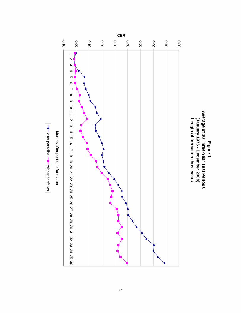
Figure 1 Average of 10 Three-Year Test Periods

(January 1976 - December 2008)

Length of formation three years

-0.10

0.00

0.10

0.20

0.30

0.40

0.50

0.60

0.70

0.80

12

34

56

78

910

1112

1314

1516

1718

1920

2122

2324

2526

2728

2930

3132

3334

3536

Months after portfolio form

ation

CER

loser portfoliosw

inner portfolios

21

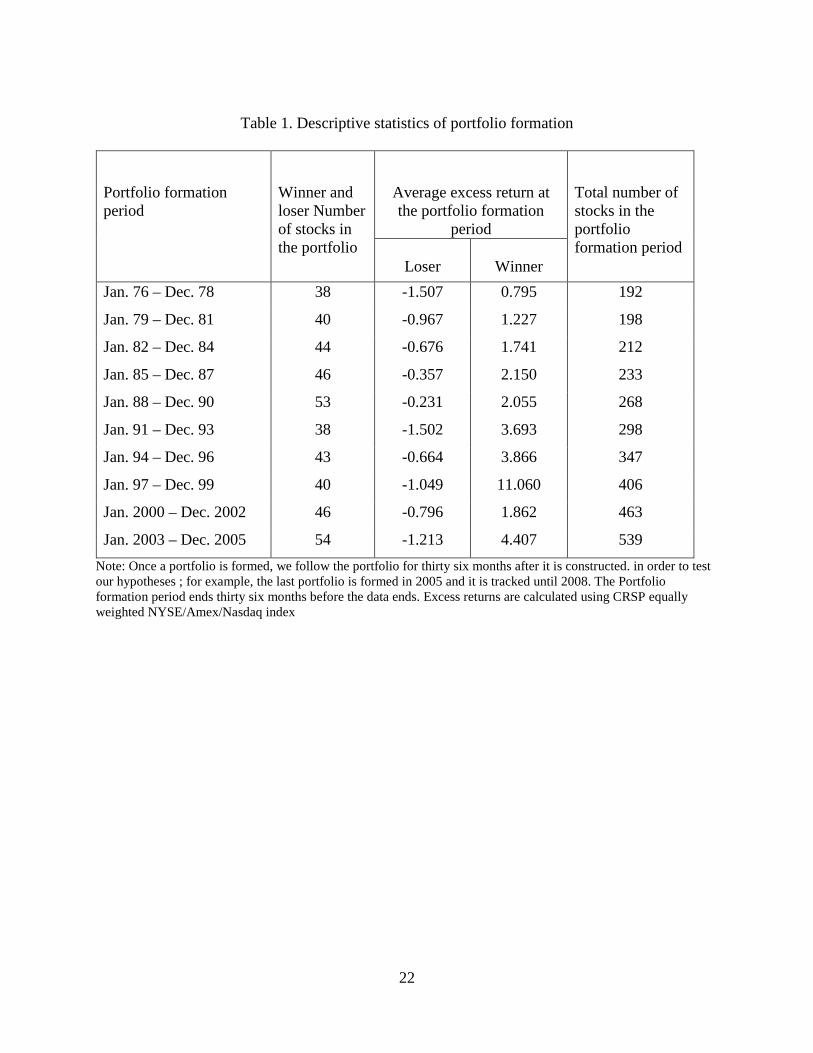
Table 1. Descriptive statistics of portfolio formation

Portfolio formation period

Winner and loser Number of stocks in the portfolio

Average excess return at the portfolio formation

period

Total number of stocks in the portfolio formation period

Loser

Winner Jan. 76 – Dec. 78 38 -1.507 0.795 192

Jan. 79 – Dec. 81 40 -0.967 1.227 198

Jan. 82 – Dec. 84 44 -0.676 1.741 212

Jan. 85 – Dec. 87 46 -0.357 2.150 233

Jan. 88 – Dec. 90 53 -0.231 2.055 268

Jan. 91 – Dec. 93 38 -1.502 3.693 298

Jan. 94 – Dec. 96 43 -0.664 3.866 347

Jan. 97 – Dec. 99 40 -1.049 11.060 406

Jan. 2000 – Dec. 2002 46 -0.796 1.862 463

Jan. 2003 – Dec. 2005 54 -1.213 4.407 539 Note: Once a portfolio is formed, we follow the portfolio for thirty six months after it is constructed. in order to test our hypotheses ; for example, the last portfolio is formed in 2005 and it is tracked until 2008. The Portfolio formation period ends thirty six months before the data ends. Excess returns are calculated using CRSP equally weighted NYSE/Amex/Nasdaq index

22

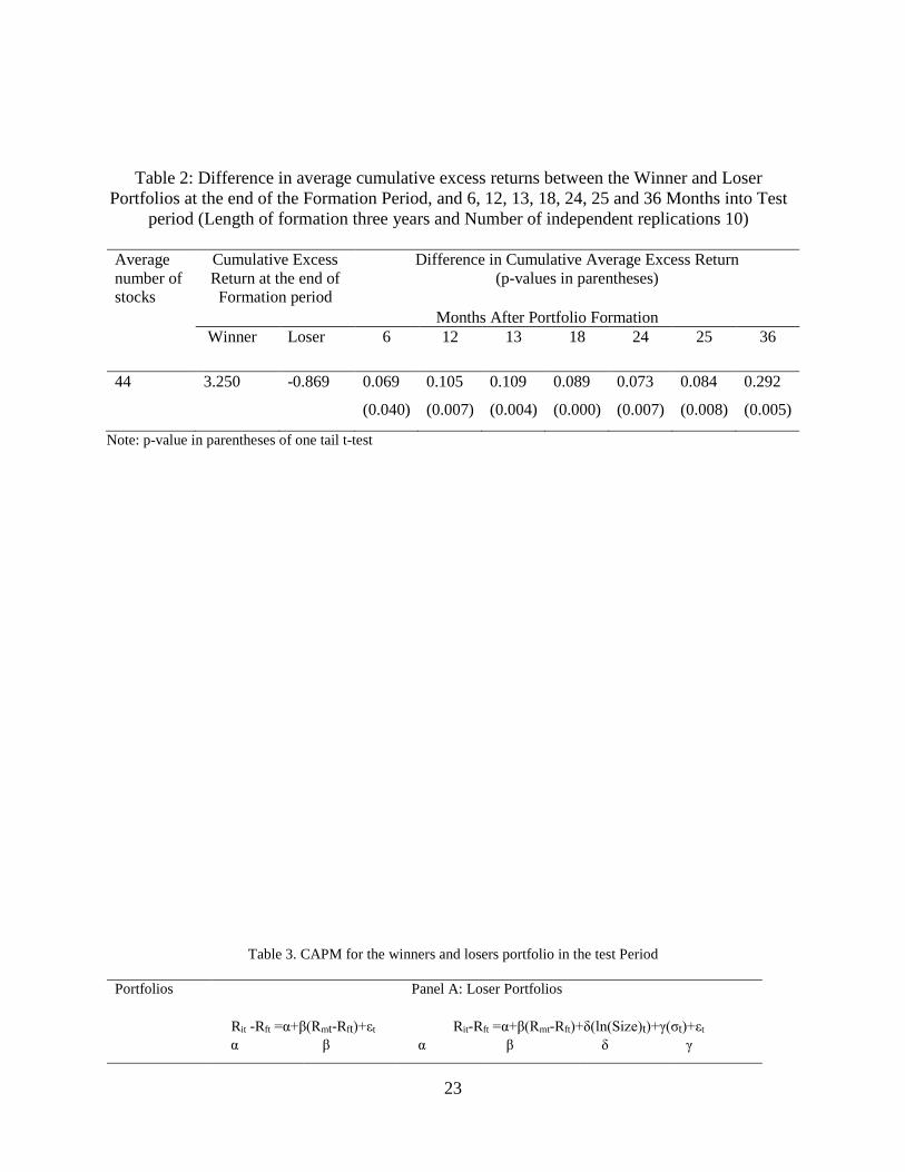
Table 2: Difference in average cumulative excess returns between the Winner and Loser Portfolios at the end of the Formation Period, and 6, 12, 13, 18, 24, 25 and 36 Months into Test

period (Length of formation three years and Number of independent replications 10)

Average number of stocks

Cumulative Excess Return at the end of Formation period

Difference in Cumulative Average Excess Return (p-values in parentheses)

Months After Portfolio Formation

Winner Loser 6 12 13 18 24 25 36

44 3.250 -0.869 0.069 0.105 0.109 0.089 0.073 0.084 0.292

(0.040) (0.007) (0.004) (0.000) (0.007) (0.008) (0.005)

Note: p-value in parentheses of one tail t-test

Table 3. CAPM for the winners and losers portfolio in the test Period

Portfolios Panel A: Loser Portfolios

Rit -Rft =α+β(Rmt-Rft)+εt Rit-Rft =α+β(Rmt-Rft)+δ(ln(Size)t)+γ(σt)+εt α β α β δ γ

23

1

2

3

4

5

6

7

8

9

10

.241 (.201) .706*** (.190) .571** (.271) .839*** (.228) 1.661 *** (.265) .832*** (.222) .200 (.552) 2.723*** (.381) 1.303*** (.308) .179 (.166)

.902*** (.042) .900*** (.044) 1.058*** (.045) 1.019*** (.058) 1.023*** (.084) .866*** (.076) 1.043*** (.064) .451*** (.066) 1.754*** (.101) .888*** (.035)

8.801*** (1.976) 2.140 (1.509) .684 (1.836) 6.597*** (1.785) 4.062** (2.024) 2.135 (1.717) -2.575 (2.696) 9.693*** (3.084) 14.707*** (2.506) -.901 (1.946)

.896*** (.041) .903*** (.044) 1.070*** (.045) .996*** (.059) 1.034*** (.085) .872*** (.077) 1.045*** (.064) .449*** (.066) 1.679*** (.100) .897*** (.038)

-.590*** (.142) -.048 (.106) -.130 (.134) -.390*** (.129) -.212 (.147) -.079 (.116) .156 (.188) -.491** (.209) -.687*** (.167) .048 (.114)

-.702 (.759) -1.554* (.867) 2.511*** (.783) -.607 (.475) -.410 (.293) -.428 (.920) .333 (.241) .037 (1.598) 1.322*** (.285) 1.190 (1.894)

Portfolios Panel B: Winner Portfolios Rit - Rft =α+β(Rmt-Rft)+εt Rit - Rft =α+β(Rmt-Rft)+δ(ln(Size))+γ(σ)+εt α β α β δ γ

1

2

3

4

5

6

7

8

9

10

1.103*** (.266) .638*** (.245) .414** (.202) .671*** (.194) .278 (.206) .135 (.277) .328 (.404) 1.453*** (.431) 1.003*** (.172) 1.614*** (.245)

1.252*** (.055) 1.169*** (.056) 1.183*** (.033) .996*** (.048) 1.254*** (.065) 1.484*** (.096) 1.383** (.075) 1.884*** (.075) .740*** (.056) 1.503*** (.052)

8.959*** (2.498) 5.659** (2.527) 5.032** (2.075) .934 (1.521) 7.377*** (1.930) -1.414 3.512) -5.474* (3.007) 17.077*** (4.689) 3.365* (1.925) 11.805*** (3.033)

1.241*** (.055) 1.180*** (.056) 1.182*** (.033) 1.010*** (.049) 1.226*** (.065) 1.568*** (.100) 1.370*** (.076) 1.883*** (.076) .736*** (.057) 1.523*** (.052)

-.621*** (.201) -.275 (.195) -.309** (.148) -.082 (.106) -.408*** (.128) .196 (.237) .327* (.192) -.901*** (.227) -.149 (.126) -.714*** (.192)

-.045 (.859) -2.086** (.825) -.290 (.340) 1.836** (.747) -.769*** (.255) -2.288*** (.005) .350* (.195) -1.312 (.037) -.149 (.766) 1.779*** (.667)

Note: Standard errors are in parentheses. *,**, *** significant at 10%, 5% and 1% level of significance. Size is market capital of the stock. The variable σ is the standard deviation of the portfolios excess return in the 36th testing period months.

Table 4. Fama-French three factor model for the winners and losers portfolio in the test Period

Portfolios Panel A: Loser Portfolios Rit -Rft =α+β(Rmt-Rft)+δ(SMBt)+γ(HMLt)+εt

α β δ γ

1 -.114 .779*** .473*** .040

24

2

3

4

5

6

7

8

9

10

(.211) .433* (.236) .678** (.280) 1.009*** (.234) .764*** (.292) .759*** (.224) .417 (.339) 1.836*** (.401) 1.307 *** (.326) .139 (.166)

(.060) .958*** (.054) 1.089*** (.057) 1.086*** (.063) 1.062*** (.090) .969*** (.083) 1.135*** (.082) .886*** (.079) 1.438*** (.126) .865*** (.037)

(.100) .099 (.098) .342** (.135) .280*** (.098) .830*** (.102) .247** (.108) .316*** (.092) .107 (.075) .649*** (.158) .078 (.079)

(.077) .178* (.092) .258* (.114) .497*** (.133) .388*** (.102) .405*** (.130) .333*** (.126) .813*** (.098) -.084 (.187) .277*** (.081)

Portfolios Panel B: Winner Portfolios Rit -Rft =α+β(Rmt-Rft)+δ(SMBt)+γ(HMLt)+εt

α β δ γ

1

2

3

4

5

6

7

8

9

10

.522* (.278) .535* (.303) .429** (.209) .655*** (.199) .725*** (.230) .352 (.279) .433 (.398) 1.689*** (.462) .818*** (.182) 1.648*** (.244)

.920*** (.079) 1.127*** (.070) 1.136*** (.042) .902*** (.054) 1.115*** (.071) 1.315*** (.104) 1.266*** (.096) 1.624*** (.091) .606*** (.070) 1.496*** (.054)

.866*** (.131) .437*** (.125) -.114 (.101) -.024 (.083) -.004 (.080) .043 (.135) .216** (.108) .138 (.086) .288*** (.088) .224* (.115)

-.255** (.101) -.005 (.118) -.228** (.107) -.527 (.113) -.399*** (.081) -.601*** (.163) -.200*** (.148) -.397*** (.114) .287*** (.105) -.683*** (.119)

Note: Standard errors are in parentheses. *,**, *** significant at 10%, 5% and 1% level of significance. Size is market capital of the stock. The variable σ is the standard deviation of the portfolios excess return in the 36th testing period months.

Table 5. Four factor model for the winners and losers portfolio in the test Period

Portfolios Panel A: Loser Portfolios Rit - Rft =α+β(Rmt-Rft)+δ(SMBt)+γ(HMLt)+ λ(MOMt) + εt

α β δ γ λ

25

1

2

3

4

5

6

7

8

9

10

.265 (.222) .436* (.253) .743*** (.280) 1.023*** (.248) .867*** (.300) .883*** (.237) .784** (.355) 1.817*** (.401) 1.289*** (.325) .332** (.169)

.906*** (.064) .957*** (.060) 1.203*** (.064) 1.082*** (.067) 1.091*** (.092) .971*** (.083) 1.060*** (.084) .841*** (.086) 1.193*** (.142) .803*** (.039)

.390*** (.100) .100 (.103) .332** (.134) .272** (.109) .800*** (.103) .227** (.109) .232** (.095) .140* (.079) .917*** (.174) .075 (.078)

-.145* (.084) .177* (.094) .407*** (.149) .487*** (.147) .393*** (.102) .366*** (.133) .057 (.150) .817*** (.098) .114 (.194) .048 (.092)

-.295*** (.058) -.003 (.077) -.349*** (.095) -.017 (.001) -.127 (.084) -.198 (.126) -.305*** (.090) -.062 (.048) -.352*** (.097) -.252*** (.049)

Portfolios Panel B: Winner Portfolios Rit -Rft =α+β(Rmt-Rft)+δ(SMBt)+γ(HMLt)+ λ(MOMt) + εt

α β δ γ λ

1

2

3

4

5

6

7

8

9

10

.521* (.295) .426 (.325) .398* (.209) .606*** (.211) .753*** (.237) .542* (.296) .953** (.416) 1.620*** (.460) .820*** (.182) 1.210*** (.246)

0.920*** (.085) 1.158*** (.077) 1.080*** (.048) .915*** (.057) 1.123*** (.072) 1.318*** (.104) 1.159*** (.099) 1.459*** (.099) .630*** (.080) 1.634*** (.056)

.866*** (.133) .398*** (.132) -.109 (.100) .004 (.093) -.012 (.082) .012 (.135) .097 (.111) .263*** (.091) .262*** (.098) .230** (.114)

-.255** (.112) .020 (.121) -.301*** (.111) -.489*** (.125) -.398*** (.081) -.661*** (.165) -.591*** (.175) -.382*** (.113) .268** (.109) -.163 (.134)

.000 (.077) .092 (.099) .171** (.071) .057 (.083) .035 (.066) -.303* (.157) -.432*** (.105) -.231*** (.055) .033 (.055) .567*** (.071)

Note: Standard errors are in parentheses. *,**, *** significant at 10%, 5% and 1% level of significance. Size is market capital of the stock. The variable σ is the standard deviation of the portfolios excess return in the 36th testing period months.

26