Overlapping resonances in the control of intramolecular vibrational redistribution

arX

iv:q

uant

-ph/

0703

263v

1 2

8 M

ar 2

007

Overlapping resonances in the control of intramolecular vibrational redistribution

D. Gerbasi1, A. S. Sanz1∗, P. S. Christopher1, M. Shapiro2, and P. Brumer11Chemical Physics Theory Group, Department of Chemistry,

and Center for Quantum Information and Quantum Control,

University of Toronto, Toronto, Canada M5S 3H6; and2Chemical Physics Department, The Weizmann Institute of Science,

Rehovot, Israel 76100, and Department of Chemistry,

University of British Columbia, Vancouver, Canada, V6T 1Z1.

(Dated: February 9, 2008)

Coherent control of bound state processes via the interfering overlapping resonances scenario[Christopher et al., J. Chem. Phys. 123, 064313 (2006)] is developed to control intramolecularvibrational redistribution (IVR). The approach is applied to the flow of population between bondsin a model of chaotic OCS vibrational dynamics, showing the ability to significantly alter the extentand rate of IVR by varying quantum interference contributions.

PACS numbers:

I. INTRODUCTION

Quantum control of molecular processes1,2 has proved,over the past two decades, to be viable both theoreticallyand experimentally. An examination of the coherent con-trol literature, wherein scenarios are expressly designedto take advantage of quantum interference phenomena,shows that the vast majority of applications has been toprocesses occurring in the continuum energy regime. Re-cently we proposed a new approach to controlling boundstate dynamics in large polyatomic molecules3 that ex-ploits interferences between overlapping resonances. Wehave demonstrated the viability of this scenario in con-trolling internal conversion in pyrazine.3,4,5 In the presentpaper we further develop this method, applying it tothe control of Intramolecular Vibrational Redistribution(IVR). As an example, we study the control of the flow ofenergy between bonds in a model of OCS. This molecule,though small, is of particular interest at high energies,where, classically, it displays predominantly chaotic dy-namics. In spite of the classical chaos, quantum controlvia the present scenario is shown to be excellent.

This paper is organized as follows: Section II providesan overview of the theory, with a discussion of the Fes-hbach partitioning technique which, as we have shown,3

provides a highly efficient method for dealing with boundstate problems. Section III describes the collinear OCSmodel and its classical dynamical characteristics. In Sec-tion IV we discuss the application of the method to thecontrol of IVR in OCS. An Appendix describes our use ofthe Feshbach partitioning technique for the numerical so-lution of the bound state problem for small systems suchas OCS. A more ambitious method for addressing consid-

∗Current address: Instituto de Matematicas y Fısica Fundamental,

Consejo Superior de Investigaciones Cientıficas, Serrano 123, 28006

Madrid, Spain

erably larger systems, the “QP algorithm”, is describedelsewhere.5

II. BOUND STATE CONTROL

A. Time-evolution of populations in molecular

systems

We consider a system described by an Hamiltonian Hwhich can be partitioned physically into the sum of twocomponents HA and HB, plus the interaction HAB be-tween them:

H = HA +HB +HAB, (1)

The eigenstates and eigenvalues of the full Hamiltonianare defined by:

H |γ〉 = Eγ |γ〉 . (2)

The (“zeroth-order”) eigenstates and eigenvalues of thesum of the decoupled Hamiltonians are defined as

(HA +HB)|κ〉 = E(κ)|κ〉 . (3)

Below, we are interested in the time evolution of the sys-tem, initially prepared in a superposition of zeroth orderstates.

|Ψ(t = 0)〉 =∑

κ

cκ|κ〉, (4)

where {cκ} are “preparation” coefficients. All sums over|κ〉, here and below, are assumed to be confined to asubspace S. For example, the selected initial states mightconsist of a set with population heavily concentrated inone bond of a molecule, in which case, energy flow out ofsuch superposition states is examined.

The time-evolution of Eq. (4) at any subsequent timecan then be obtained by expanding the (zeroth order)

2

eigenstates, |κ〉, in terms of the exact eigenstates |γ〉 togive:

|Ψ(t)〉 =∑

κ,γ

cκa∗κ,γe

−iEγt/~|γ〉, (5)

with a∗κ,γ = 〈γ|κ〉. The structure of |〈γ|κ〉|2 as a functionof γ defines a resonance shape that provides insight, inthe frequency domain, into the population flow out andinto the zeroth order |κ〉 states.

Given this time evolution, the amplitude for findingthe system in a state |κ〉 at time t is

cκ = 〈κ|Ψ(t)〉 =∑

κ′

cκ′Mκ,κ′(t), (6)

where

Mκ,κ′(t) ≡∑

γ

aκ,γa∗κ′,γe

−iEγt/~

= 〈κ|

(∑

γ

e−iEγt/~|γ〉〈γ|

)|κ′〉 (7)

is the (κ, κ′) element of the overlap matrix M(t) definedby the term in brackets in Eq. (7). Note that, for κ′ 6= κ,if the states |κ〉 and |κ′〉 do not overlap with a com-mon |γ〉, i.e., there are no overlapping resonances, thenMκ,κ′ = 0. Our previous studies3 have demonstrated thesignificance of such overlapping resonances to the controlof radiationless transitions, such as internal conversion.

From Eq. (6), the probability of finding the system ina collection of states |κ〉 contained in the initial set S attime t is given by

P (t) =∑

κ

|〈κ|Ψ(t)〉|2 = c†K(t)c, (8)

where c is a κ-dimensional vector whose components arethe cκ coefficients, and K(t) ≡ M

†(t)M(t). The gen-eralization to the question of finding population in analternative collection of states, other than S, is straight-forward. However, it is unnecessary for the study below,as will become evident. Equation (8) allows us to ad-dress the question of enhancing or restricting the flow ofprobability out of S by finding the optimal combinationof cκ that achieves this goal at a specified time T . Ex-perimentally, the resultant required superposition statecan be prepared using modern pulse shaping techniques.

B. The Feshbach partitioning technique

Our interest is to control the flow of population out ofsome generic molecular subspace into the entire molec-ular Hilbert space. In order to do so we make useof the bound state version of the Feshbach partition-ing technique.6,7 Here, since the control approach is be-ing tested on a small system, we solve the resulting

equations in a straightforward way, as described in Ap-pendix A. Larger systems can take advantage of the “QPalgorithm”.5

The Feshbach partitioning technique is based on defin-ing two projection operators

Q ≡∑

κ

|κ〉〈κ|, P ≡∑

β

|β〉〈β|, (9)

which satisfy the following properties:

Q2 = Q, P 2 = P, (10a)

[Q,P ] = 0, (10b)

P +Q = I, (10c)

where I is the identity operator. In what follows, theflow of probability of interest is from the Q space to theP space.

Using Eqs. (10c) and (9), the eigenstates of the fullHamiltonian can be written as

|γ〉 =∑

κ

|κ〉〈κ|γ〉 +∑

β

|β〉〈β|γ〉. (11)

Similarly, the Schrodinger equation can be expressed as

[Eγ −H ][P +Q]|γ〉 = 0, (12)

whereby multiplying it by P and then by Q, and usingEq. (10), one obtains the following set of coupled equa-tions:

[Eγ − PHP ]P |γ〉 = PHQ|γ〉, (13a)

[Eγ −QHQ]Q|γ〉 = QHP |γ〉. (13b)

The states |κ〉 and |β〉 are solutions to the decoupled(homogeneous) equations arising from Eqs. (13a) and(13b), respectively. That is,

[Eβ − PHP ]P |β〉 = 0, (14a)

[Eκ −QHQ]Q|κ〉 = 0. (14b)

Contrary to continuum problems, in general Eγ 6= Eβ

and it is possible to express P |γ〉 in terms of the partic-ular solution of the (inhomogeneous) Eq. (13a),

P |γ〉 = [Eγ − PHP ]−1PHQ|γ〉. (15)

Substituting Eq. (15) into Eq. (13b) results in

[Eγ −QHQ]Q|ψ〉 = QHP [Eγ −PHP ]−1PHQ|ψ〉. (16)

By rearranging terms in this equation, one obtains

[Eγ −H]Q|γ〉 = 0, (17)

where H is an effective Hamiltonian, defined as

H = QHQ+QHP [Eγ − PHP ]−1PHQ. (18)

3

i Di βi R0i

1 0.08518 1.5000 2.9759

2 0.21238 1.6251 2.2559

3 0.16000 1.1589 2.8037

TABLE I: Parameters defining the potential energy surfacegiven by Eq. (32). All magnitudes are given in a.u.

The term between squared brackets can be written as

[Eγ − PHP ]−1

=∑

β

1

Eγ − Eβ|β〉〈β| (19)

by using the spectral resolution of an operator. The ma-trix elements of H are given by

〈κ|H|κ′〉 = Eκδκ,κ′ + ∆κ,κ′ , (20)

where

∆κ,κ′ =1

2π

∑

β

Γκ,κ′

Eγ − Eβ, (21a)

Γκ,κ′ = 2πV (κ|β)V (β|κ′), (21b)

with V (κ|β) = 〈κ|QHP |β〉 being the coupling term.Equations (21a) and (21b) represent the energy shift andthe decay rate, respectively. By diagonalizing Eq. (17) ina self-consistent manner, one obtains the energy eigen-values, Eγ , and the values for the overlap integrals, aκ,γ .

Note that the energy eigenvalues and the overlap in-tegrals can also be obtained8 by directly diagonalizingthe full Schrodinger equation in the zeroth-order basis.However, the partitioning technique presented above hascomputational advantages for cases where the dimensionsof the P space is large, since one only needs to diagonal-ize an effective Hamiltonian H with dimensions given bythe Q space. Note, however, that diagonalizing H re-quires using iterative procedures, and needs to be solvedrepeatedly until each eigenvalue is found. Appendix Aprovides details on the partitioning algorithm used here.

C. Optimal Control

To determine the set of optimal preparation coefficientsleading to either a maximum or a minimum population attime t = T , we need to find the extrema of the function9

Pλ(t) = c†K(t)c − λc†c (22)

with respect to the coefficients c, where λ is a Lagrangemultiplier added to assure normalization, i.e.,

∑

κ

|cκ|2 = 1. (23)

The optimum vector, cT , is obtained by differentiatingEq. (22) with respect to the components of c†, and equat-ing the resulting expression to zero at time T , i.e.,

∂Pλ(t)

∂c∗κ′

∣∣∣∣t=T

=∑

κ

Kκ′,κ(T )cκ − λcκ = 0. (24)

The optimum vector resulting from this procedure is a so-lution to the eigenvalue problem represented by Eq. (24).Note that this vector can either maximize or minimizethe solution. In the first case, the interference betweenoverlapping resonances created by the initial superposi-tion will be seen to result in a delay of the populationdecay, whereas in the second case the population decayis being accelerated.

In order to further clarify the dependence of the time-evolution on overlapping resonances, Eq. (8) can be re-expressed as

P (t) =∑

κ

|cκ|2gκ +

∑

κ′,κκ′ 6=κ

c∗κ′cκfκ′,κ, (25)

where

gκ =∑

κ′

|Mκ′,κ|2, (26)

and

fκ′,κ =∑

κ′′

M∗κ′′,κ′Mκ′′,κ. (27)

As expressed in Eq. (25), the Q space population assumesthe generic coherent control form1,2: it is given as thesum of non-interfering pathways, represented by gκ′ , andinterfering pathways, represented by fκ′,κ.

D. The Role of Overlapping Resonances

The interference term in Eq. (25) depends on fκ′,κ,which, in accord with Eq. (27), depends upon the over-lap between resonances. Qualitatively speaking, a reso-nance is described by bound states |κ〉 coupled to a quasi-continuum of exact eigenstates |γ〉. Each such state isthus associated with the energy width of the 〈κ|γ〉 over-lap coefficients. Overlapping resonances are the result ofhaving at least two states whose resonance widths arewider than their associated level spacing. The resultingresonances interfere with one another, displaying a vari-ety of lineshapes,2 and are responsible for the interferencein this control scenario. In the absence of overlappingresonances the full fκ′,κ-term in Eq. (25) vanishes andcontrol disappears.

Note that there are also contributions from overlap-ping resonances to the gκ-term, as can be seen from their

4

effect on the nature of the decay from the individual |κ〉.These resonances distort the lineshape, and hence thecorresponding time dependence. In order to determinethe contribution from overlapping resonances, we havedevised3 a qualitative measure, defined as

P (t) = [P (t) −W (t)], (28)

where

W (t) =∑

κ

|cκMκ,κ|2. (29)

Here W (t) is a measure of the direct contribution, and

P (t) provides a measure of the overlapping resonancecontribution. In the absence of overlapping resonances,P (t) = W (t).

III. CLASSICAL ASPECTS OF THE

COLLINEAR OCS

A. The OCS model

As a working model to illustrate the usefulness of themethod described in Sec. II, we consider a collinear modelof OCS, with a modified Sorbie-Murrell10 potential. Theinterest in this system arises from the fact that, close todissociation, i.e. in the energy region of interest below,the classical dynamics becomes highly chaotic. As such,collinear OCS is a complex system with a penchant forextensive IVR.

The classical dynamics of OCS has been studied inboth planar,10 and collinear11,12 versions. Here, we con-sider the collinear case, which is described by the Hamil-tonian

H =P 2

1

2µ13+

P 22

2µ23−P1P2

mC+ V (R1, R2, R3), (30)

where

µ13 =mOmC

mO +mC

µ23 =mSmC

mS +mC, (31)

are reduced masses; R1 and R2 are the CS and CO bonddistances, respectively (R3 = R1 + R2); and P1 and P2

are the corresponding momenta.

In the course of this work we found that the Sorbie-Murrell OCS model10 displayed a second minimum atlarge distances along both the CS and CO exit channels.Although the depth of this second well is extremely small,there are a large number of closely packed eigenstates lo-calized in this region due to the length of the well. To ourknowledge, there is no experimental evidence to eithersupport or refute a second minimum, although they have

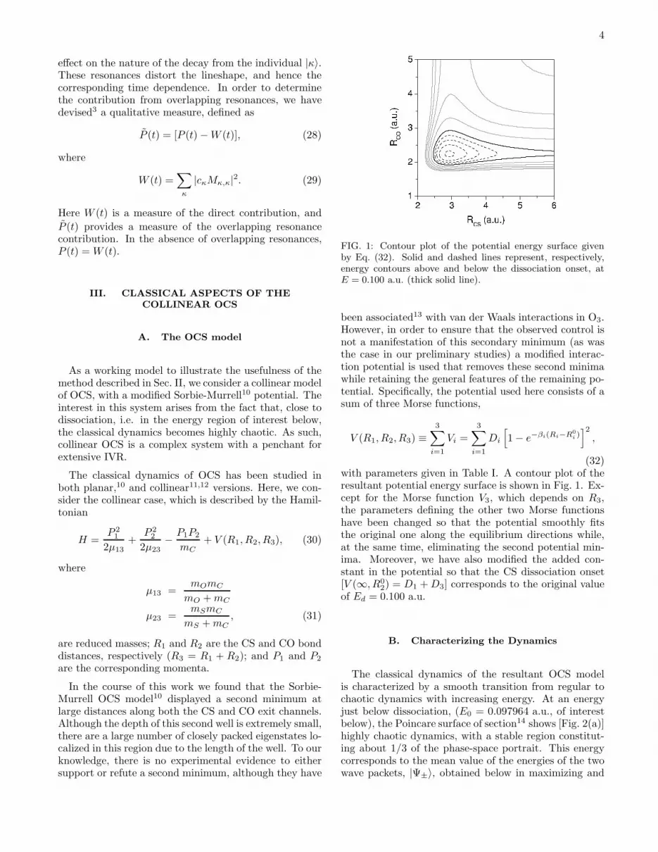
FIG. 1: Contour plot of the potential energy surface givenby Eq. (32). Solid and dashed lines represent, respectively,energy contours above and below the dissociation onset, atE = 0.100 a.u. (thick solid line).

been associated13 with van der Waals interactions in O3.However, in order to ensure that the observed control isnot a manifestation of this secondary minimum (as wasthe case in our preliminary studies) a modified interac-tion potential is used that removes these second minimawhile retaining the general features of the remaining po-tential. Specifically, the potential used here consists of asum of three Morse functions,

V (R1, R2, R3) ≡

3∑

i=1

Vi =

3∑

i=1

Di

[1 − e−βi(Ri−R0

i )]2,

(32)with parameters given in Table I. A contour plot of theresultant potential energy surface is shown in Fig. 1. Ex-cept for the Morse function V3, which depends on R3,the parameters defining the other two Morse functionshave been changed so that the potential smoothly fitsthe original one along the equilibrium directions while,at the same time, eliminating the second potential min-ima. Moreover, we have also modified the added con-stant in the potential so that the CS dissociation onset[V (∞, R0

2) = D1 +D3] corresponds to the original valueof Ed = 0.100 a.u.

B. Characterizing the Dynamics

The classical dynamics of the resultant OCS modelis characterized by a smooth transition from regular tochaotic dynamics with increasing energy. At an energyjust below dissociation, (E0 = 0.097964 a.u., of interestbelow), the Poincare surface of section14 shows [Fig. 2(a)]highly chaotic dynamics, with a stable region constitut-ing about 1/3 of the phase-space portrait. This energycorresponds to the mean value of the energies of the twowave packets, |Ψ±〉, obtained below in maximizing and

5

FIG. 2: (a) Poincare surface of section for the collinear OCSmodel at E = 0.09796 a.u. The solid line represents the totalenergy contour. (b) Distance between two nearby trajecto-ries (with d0 = 10−8 a.u.) chosen in the stable region (H),and in the chaotic sea (N). The high-frequency oscillationshave been averaged out in both cases (the smoothing causes

Λ(H) to appear as if it does not begin at zero). (c) CS–bondvibrational energy corresponding to the chaotic trajectory ofpart (b).

minimizing the energy flow from the CS bond. Surfacesof section in the nearby energies are essentially similar.This being the case, there is no obvious classical originto the control of bond energy relaxation described below.Of some future interest, however, might be an auxiliarystudy of the relationship of overlapping resonances in-duced control, observed below, to classical features suchas bond energy recurrences, cantori, and the inhomoge-neous character of the OCS phase space11,12,15,16,17,18.

Quantitative insight into the rate of loss of correlationsin the chaotic region of phase space can be obtained bycomputing Lyapunov exponents,19 approximated by theaverage (over various trajectories) of the exponential rateat which the distance d(t) between adjacent trajectories

in phase space grow in time:

λ∞ = limt→∞

1

tlnd(t)

d0. (33)

Here, in order to show how different regular and chaotictrajectories behave, we have computed the quantity

Λ(t) = lnd(t)

d0, (34)

with d0 = 10−8 a.u. We label the finite time Lyapunovexponent, computed in this way, as λt.

The quantity Λ(t) is shown in Fig. 2(b) for two setsof nearby trajectories,20 picked in two different regionsof phase-space: the stable island, and the chaotic sea.

The results, to t ≈ 1.2 ps, give λ(stable)t ≃ 1.46 ps−1, and

λ(chaotic)t ≃ 17.41 ps−1 in the regular and chaotic regions,

respectively. The associated times are to be comparedto zeroth order vibrational periods (27.45 fs for the CSbond, and 18.10 fs for the CO bond).

Finally, in Fig. 2(c) we show the energy in the CS bond,for a trajectory in the chaotic sea. As can be seen, theenergy displays a complicated pattern, with irregular en-ergy transfer between both bonds as a function of time.Nonetheless, when one computes the energy average ofan ensemble of trajectories, the pattern becomes smoothand displaying a profile than can be fitted to an expo-nential decay,12 similar to those observed in its quantumcounterpart below.

IV. COHERENT CONTROL OF IVR

A. Population decay

We now consider the suppression (and enhancement)of IVR in the above model of OCS. Our intent is to assessthe extent of control in such a system, and to establishthe relationship between control and overlapping reso-nances. The coupling terms V (κ|β) and, subsequently,the overlap integrals aκ,γ and the energy eigenvalues Eγ

are calculated by expanding the OCS wave functions inproducts of the zeroth order states,

|Ψ〉 =∑

m,n

|ηmCS〉 ⊗ |ξn

CO〉dmn . (35)

where |ηmCS〉 and |ξn

CO〉 are eigenstates of the uncoupledCS and CO bond potentials, respectively, with quantumnumbers m and n. Our interest is in the flow, for ex-ample, out of the CS bond. Hence, the Q subspace ischosen to represent all wave functions containing onlyexcitation in the CS bond, i.e., |κ〉 are |ηm

CS〉 ⊗ |ξ0CO〉,for all m, whereas the P subspace spans the space repre-sented by all other zeroth order excitations, i.e., the |β〉

6

IVR suppression IVR enhancement

κ Eκ (a.u.) crκ ci

κ |cκ|2 cr

κ ciκ |cκ|

2 tδ (fs)

1 0.0851446 0.02895 0.00000 0.00084 − 0.13839 0.00000 0.01915 17.84

2 0.0850268 − 0.00706 0.17289 0.02994 0.38027 − 0.00806 0.14467 8.03

3 0.0848265 0.16188 − 0.16611 0.05380 − 0.00128 − 0.10472 0.01097 16.25

4 0.0845437 − 0.56608 0.25828 0.38716 0.01257 − 0.08349 0.00713 20.76

5 0.0841783 0.18017 − 0.24251 0.09127 − 0.03560 0.05674 0.00449 13.69

6 0.0837303 0.20267 0.15178 0.06411 0.19804 0.05108 0.04183 34.02

7 0.0831998 − 0.21171 0.16534 0.07216 0.12120 − 0.63185 0.41392 20.53

8 0.0825867 0.25004 − 0.41477 0.23455 0.20859 − 0.39177 0.19699 25.32

9 0.0818910 − 0.05482 0.25131 0.06616 0.24895 − 0.31440 0.16082 22.95

TABLE II: Values corresponding to the eigenstates for the (uncoupled) CS bond used in the optimized superpositions. Eκ

denotes the energy associated to these eigenstates; crκ and ci

κ are the real and imaginary parts of the cκ coefficients, respectively;and tδ is the decay time (see text for details). The optimization to maximize/minimize the energy transfer into the CO bond(suppression/enhancement of IVR) has been carried out at T = 100 fs. The energy corresponding to the ground state in the(uncoupled) CO bond is E0

CO = 0.00360475 a.u.

are |ηmCS〉 ⊗ |ξn

CO〉, n 6= 0, describing excitation in the CSbond. Initiating excitation within Q and watching theflow into P then corresponds to an experiment whereinexcitation flows out of the CS bond.

As seen in Sec. III A, the coupling term, QHP , nec-essary to obtain the energy shifts and decay rates, con-sists of a static term (V3), and a dynamic term [propor-tional to p1p2 in Eq. (30)]. The overlap integrals andenergy eigenvalues are obtained by self-consistent diago-nalization of Eq. (17). All vibrational states, |ηm

CS〉 and|ξn

CO〉, are numerically calculated using a discrete vari-able representation (DVR) technique,21 obtaining a totalof 45 eigenvectors for the CS bond, and 59 for the CObond. The number of eigenvectors is larger in the secondcase, because the dissociation threshold of the CO bondis higher in energy.

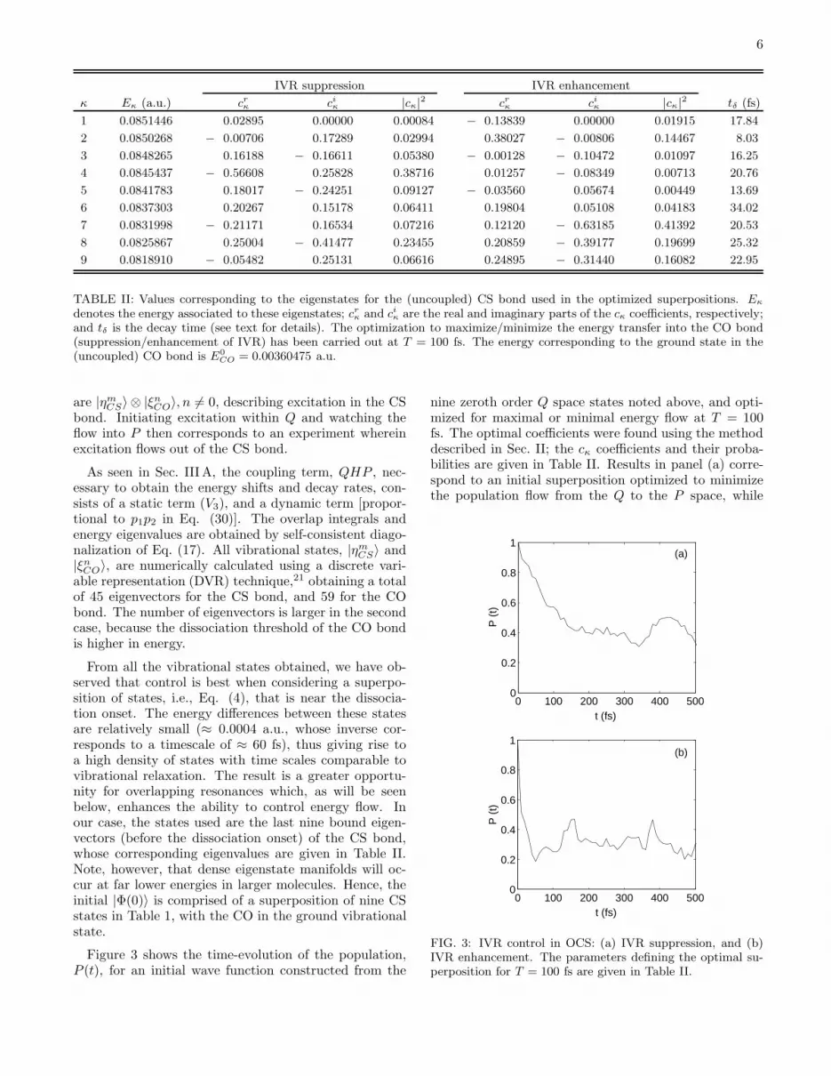
From all the vibrational states obtained, we have ob-served that control is best when considering a superpo-sition of states, i.e., Eq. (4), that is near the dissocia-tion onset. The energy differences between these statesare relatively small (≈ 0.0004 a.u., whose inverse cor-responds to a timescale of ≈ 60 fs), thus giving rise toa high density of states with time scales comparable tovibrational relaxation. The result is a greater opportu-nity for overlapping resonances which, as will be seenbelow, enhances the ability to control energy flow. Inour case, the states used are the last nine bound eigen-vectors (before the dissociation onset) of the CS bond,whose corresponding eigenvalues are given in Table II.Note, however, that dense eigenstate manifolds will oc-cur at far lower energies in larger molecules. Hence, theinitial |Φ(0)〉 is comprised of a superposition of nine CSstates in Table 1, with the CO in the ground vibrationalstate.

Figure 3 shows the time-evolution of the population,P (t), for an initial wave function constructed from the

nine zeroth order Q space states noted above, and opti-mized for maximal or minimal energy flow at T = 100fs. The optimal coefficients were found using the methoddescribed in Sec. II; the cκ coefficients and their proba-bilities are given in Table II. Results in panel (a) corre-spond to an initial superposition optimized to minimizethe population flow from the Q to the P space, while

0 100 200 300 400 5000

0.2

0.4

0.6

0.8

1

t (fs)

P (

t)

0 100 200 300 400 5000

0.2

0.4

0.6

0.8

1

t (fs)

P (

t)

(a)

(b)

FIG. 3: IVR control in OCS: (a) IVR suppression, and (b)IVR enhancement. The parameters defining the optimal su-perposition for T = 100 fs are given in Table II.

7

0 100 200 300 400 5000

0.2

0.4

0.6

0.8

1P

1

P (

t)

0 100 200 300 400 5000

0.2

0.4

0.6

0.8

1P

2

0 100 200 300 400 5000

0.2

0.4

0.6

0.8

1P

3

0 100 200 300 400 5000

0.2

0.4

0.6

0.8

1P

4

P (

t)

0 100 200 300 400 5000

0.2

0.4

0.6

0.8

1P

5

0 100 200 300 400 5000

0.2

0.4

0.6

0.8

1P

6

0 100 200 300 400 5000

0.2

0.4

0.6

0.8

1P

7

P (

t)

t (fs)

0 100 200 300 400 5000

0.2

0.4

0.6

0.8

1P

8

t (fs)

0 100 200 300 400 5000

0.2

0.4

0.6

0.8

1P

9

t (fs)

FIG. 4: Individual decay for wave functions consisting of each individual eigenvector used in the construction of the optimalsuperpositions. The labels correspond to those given in Table II.

panel (b) shows results optimized to enhance the flow ofpopulation. As is clearly seen, the initial falloff in panel(a) is much slower than that in (b). To quantify thisdecay, the initial P (t) falloff was fit to an exponentiallydecreasing function,

P (t) = P∞ + (1 − P∞)e−t/tδ , (36)

where tδ is the decay time, and P∞ is the average aroundwhich P (t) fluctuates for the first 1.0 ps. Note that thetδ values can only be regarded as approximate since thefalloff is, in general, not exponential, and tδ depends onthe time scale over which the exponential is fit. (Herethe fit is over 400 fs). In case (a), the decay time istδ ≃ 57.35 fs, while in case (b) it is tδ ≃ 8.60 fs, aboutseven times smaller. Furthermore, we note that in panel(a), only about 24% of the population has been trans-ferred from Q to P during the first 50 fs, while, in con-trast, approximately 82% of the population has beingtransferred to the P in panel (b) during the same time.Moreover, the population that asymptotically remains lo-calized along the CS bond is also larger in the case ofIVR suppression (P∞ ≃ 0.4) than in that of enhance-ment (P∞ ≃ 0.3).

The controlled results should be compared to the nat-ural IVR behavior of the individual levels participatingin the superposition. To this end, the P (t) for each ofthe participating levels is shown in Fig. 4. Although theenergy difference between these states shown is relativelysmall, the populations, Pκ, evolve with a range of initialfalloff values, as can be seen in the corresponding val-ues of tδ, given in Table II. Note also, from this table,that the control seen in Fig. 3 is not due to the identifi-cation of a particular |κ〉 that independently maximizesor minimizes the decay. Indeed, by inspecting the valueof the cκ coefficients, we find, in the case of IVR sup-pression, participation of most of the nine levels, with ≈60% of the total initial population concentrated in thetwo states with κ = 4 and κ = 8. Neither of these twostates independently have the longest decay times, buttheir interference is crucial to control. Similar observa-tions result from considering the data for optimized IVRenhancement, despite the fact that κ = 2 has a relativelysmall tδ. In this case the optimized superposition alsogives a significantly smaller P (T ) than does the individ-ual κ = 2 state.

A qualitative measure P (t) of the contribution from

8

0 100 200 300 400 5000

0.2

0.4

0.6

0.8

1

t (fs)

P (

t)

0 100 200 300 400 5000

0.2

0.4

0.6

0.8

1

t (fs)

P (

t)

(a)

(b)

FIG. 5: Contribution of P (t) (dashed line) and W (t) (dottedline) to: (a) IVR suppression, and (b) IVR enhancement.The solid line represents the corresponding P (t) function fromFigs. 3.

the interference of overlapping resonances, and W (t)from the direct contribution, was provided in Eq. (28).

Results for P (t) and W (t) for the maximization and min-imization cases above are provided in Fig. 5 where thecontribution from overlapping resonances (dashed line),become dominant after the first 10 fs, thus demonstratingthe important role played by these resonances in the IVRcontrol scenario. This is seen to be the case for both themaximization, as well as minimization, of the flow fromthe CS bond.

A pictorial, and enlightening, view of the results is pro-vided in Figs. 6 and 7, where the wave packets associatedwith IVR suppression and enhancement are shown. Ascan be seen in Fig. 6, for the case of IVR suppression,the wave packet remains highly localized along the RCS

mode, with minimum spreading along the RCO mode. Inparticular, it undergoes a slight oscillation along the RCS

mode, concentrating most of the probability around theregion where the CS dissociation takes place, in a clearcorrespondence to what happens with a classical counter-part. For the case of IVR enhancement, the effect is theopposite. As can be seen in Fig. 7, the spreading of thewave packet along the RCO mode coordinate is relativelyfast.

The method described above is, of course, applicableat any time during the dynamics. For example, we tried,

2 4 6 8 101.5

2

2.5

3

RCS

RC

O

t = 0 fs

2 4 6 8 101.5

2

2.5

3

RCS

RC

O

t = 20 fs

2 4 6 8 101.5

2

2.5

3

RCS

RC

O

t = 40 fs

2 4 6 8 101.5

2

2.5

3

RCS

RC

O

t = 60 fs

2 4 6 8 101.5

2

2.5

3

RCS

RC

O

t = 80 fs

2 4 6 8 101.5

2

2.5

3

RCS

RC

O

t = 100 fs

FIG. 6: Wave packet evolution corresponding to IVR suppres-sion. Dashed lines represent equipotential energy contours,with the innermost corresponding to the wave packet energy,E+ = 0.09849 a.u.

and successfully attained, control for times at long as1.5 ps (corresponding to over 50 CS vibrational periods),resulting in about a 55% of the population localized inthe CS bond for IVR suppression, and about 22% forIVR enhancement.

V. COMMENTS AND SUMMARY

In this paper, a method for controlling intramolecu-lar vibrational redistribution has been developed and hasbeen applied to OCS, where extensive control over IVRis attained. Of particular interest is that the control isachieved even though the associated classical dynamicsis chaotic. The method, wherein the coefficients of aninitial superposition of zeroth order states are optimized,is shown to rely upon the presence of overlapping reso-nances, a feature which is expected to be ubiquitous inrealistic molecular systems.

We have assumed throughout this paper that the ini-tial state that optimizes the intramolecular vibrational

9

2 4 6 8 101.5

2

2.5

3

RCS

RC

0t = 0 fs

2 4 6 8 101.5

2

2.5

3

RCS

RC

0

t = 20 fs

2 4 6 8 101.5

2

2.5

3

RCS

RC

0

t = 40 fs

2 4 6 8 101.5

2

2.5

3

RCS

RC

0

t = 60 fs

2 4 6 8 101.5

2

2.5

3

RCS

RC

0

t = 80 fs

2 4 6 8 101.5

2

2.5

3

RCS

RC

0

t = 100 fs

FIG. 7: Wave packet evolution corresponding to IVR en-hancement. Dashed lines represent equipotential energy con-tours, with the innermost corresponding to the wave packetenergy, E− = 0.09743 a.u.

redistribution can be prepared, for a real molecule, usingmodern pulse shaping techniques. Computations display-ing the resultant field were not, however, carried out onthis OCS model since they are best done using more re-alistic molecular potentials in higher dimensions, yield-ing realistic optimizing fields. Work of this kind is inprogress.

Acknowledgments

We thank the Natural Sciences and Engineering Re-search Council of Canada for support of this research.

APPENDIX A: NUMERICAL

IMPLEMENTATION

Here, we provide a route to compute the eigenvaluesand overlap integrals via Eq. (17). We start by definingNκ and Nβ to be the basis-set dimensions in the Q and P

space, respectively, and NT = Nκ +Nβ . The probabilityof being in the Q space, P (t), is given by Eq. (8). In orderto find P (t), two sets of values are needed: the set ofeigenvalues {Eγ}, and the overlap integrals aκ,γ betweenthe zeroth-order states in Q and the exact eigenstates |γ〉.The partitioning algorithm described below is ingeniousin the sense that it allows one to concentrate specificallyon obtaining these two sets of values. The method is wellsuited to small systems.

Beginning with Eq. (17), and using Eqs. (21), the al-gorithm is as follows:

1. Choose a starting energy Ei=0γ , with i correspond-

ing to the ith iteration. In particular, one maychoose an energy close to the zeroth-order energies.

2. Take Eiγ from the last iteration, and compute

H(Eiγ).

3. Diagonalize H(Eiγ), and select one of its eigenvalues

to be the next trial energy, Ei+1γ .

4. If |Ei+1γ − Ei

γ | ≇ 0, go back to step 2.

5. If |Ei+1γ − Ei

γ |∼= 0, Ei+1

γ becomes the eigenvaluesEγ , and its corresponding eigenvector, |Dγ〉, is pro-portional to Q|γ〉.

6. Repeat steps 1-5 until all NT unique eigenvaluesEγ are obtained.

In the process of diagonalizing the effective Hamilto-nian, H, each eigenvector |Dγ〉 has been normalized to1. Therefore, the use of the algorithm leads to a loss ofinformation about Q|γ〉. This makes necessary to alsocompute the constant of proportionality between Q|γ〉and |Dγ〉. This is done by requiring that 〈γ|γ〉 = 1 forthe full eigenvectors. Thus, one can assert that

Q|γ〉 = Cγ |Dγ〉, (A1)

with Cγ being the proportionality constant. The problemthen reduces to finding the Cγ associated with each Eγ .This is accomplished by expressing 〈γ|γ〉 as

〈γ|γ〉 = 〈γ|Q|γ〉 + 〈γ|P |γ〉

= 〈γ|Q2|γ〉 + 〈γ|P 2|γ〉, (A2)

where

〈γ|Q2|γ〉 = |Cγ |2〈Dγ |Dγ〉 = |Cγ |

2, (A3)

and, using Eq. (15),

〈γ|P 2|γ〉 = 〈γ|QHP [Eγ − PHP ]−1

× [Eγ − PHP ]−1PHQ|γ〉. (A4)

The application of the spectral resolution of an operator,Eq. (19), to Eq. (A4) leads to

〈γ|P 2|γ〉 =∑

β

〈γ|QH |β〉〈β|HQ|γ〉(Eγ − Eβ

)2 , (A5)

10

whereby, by making use of Eq. (A1), one obtains

〈γ|P 2|γ〉 = |Cγ |2∑

β

〈Dγ |H |β〉〈β|H |Dγ〉(Eγ − Eβ

)2 . (A6)

Now 〈γ|P 2|γ〉 is easily computed by realizing that

〈Dγ |H |β〉 =∑

κ

D∗κγ〈κ|H |β〉 (A7)

=∑

κ

D∗κγV (κ|β). (A8)

The substitution of Eqs. (A3) and (A6) into Eq. (A2)yields

〈γ|γ〉 = 1 = |Cγ |2

1 +∑

β

∣∣∑κD

∗κγV (κ|β)

∣∣2(Eγ − Eβ

)2

, (A9)

from which one obtains the proportionality factor |Cγ |.

According to the procedure previously described, wecan determine Q|γ〉, given |Dγ〉, with the exception of aconstant phase factor. Note that, in general, each pro-portionality factor, Cγ , can be written as |Cγ |e

θγ , whereθγ is a random phase. However, this is not a problemsince the results are independent of any constant phasefactor; as seen from Eq. (7), all overlap integrals appearin pairs, aκ′,γa

∗κ,γ , which can be expressed as

〈κ|γ〉〈γ|κ′〉 = 〈κ|eiθγ |γ〉〈γ|e−iθγ |κ′〉

= 〈κ|γ〉〈γ|κ′〉. (A10)

1 S. A. Rice and M. Zhao, in Optical Control of Molecular

Dynamics (Wiley, New York, 2000).2 M. Shapiro and P. Brumer, in Principles of the Quantum

Control of Molecular Processes (Wiley, New York, 2003).3 P. S. Christopher, M. Shapiro, and P. Brumer, J. Chem.

Phys. 123, 064313 (2005).4 P. S. Christopher, M. Shapiro, and P. Brumer, (to be pub-

lished) extends the treatment in References 3 and 5 totwenty-four mode Pyrazine.

5 P. S. Christopher, M. Shapiro and P. Brumer, J. Chem.Phys. 124, 184107 (2006).

6 H. Feshbach, Ann. Phys. (N.Y.) 19, 287 (1962); 43, 410(1967).

7 R.D. Levine, Quantum Mechanics of Molecular Rate Pro-

cesses (Clarendon Press, Oxford, 1969).8 D. Gerbasi, Ph.D. Dissertation, University of Toronto

(2004).9 E. Frishman and M. Shapiro, Phys. Rev. Lett. 87, 253001

(2001).10 D. Carter and P. Brumer, J. Chem. Phys. 77, 4208 (1982).11 M.J. Davis, Chem. Phys. Lett. 110, 491 (1984).12 M.J. Davis, J. Chem. Phys. 83, 1016 (1985).13 R. Siebert, R. Schinke, and M. Bittererova, PCCP Com-

munications 3, 1795 (2001).14 The surface of section has been computed in the standard

way, i.e., by following each trajectory, and noting R1 andP1 each time that R2 crosses the surface R2 = R0

2 withP2 > 0.

15 B. Eckhardt, Phys. Rep. 163, 205 (1988).16 B.V. Chirikov, J. Nucl. Energy C 1, 253 (1960); Phys. Rep.

52C, 265 (1979).17 R.C. Brown and R.E. Wyatt, Phys. Rev. Lett. 57, 1 (1986);

J. Phys. Chem. 90, 3590 (1986).18 L.L. Gibson, G.C. Schatz, M.A. Ratner, and M.J. Davis,

J. Chem. Phys. 86, 3263 (1987).19 A.J. Lichtenberg and M.A. Lieberman, Regular and

Stochastic Motion (Springer-Verlag, Berlin, 1983).20 Perturbed trajectories were designed in the traditional

manner, modifying slightly R1 (R1 → Rδ1 = R1 + δ) and

adjusting P2 to restore the original energy.21 J.V. Lill, G.A. Parker, and J.C. Light, Chem. Phys. Lett.

89, 483 (1982); J.C. Light, I.P. Hamilton, and J.V. Lill, J.Chem. Phys. 82, 1400 (1985); S.E. Choi and J.C. Light, J.Chem. Phys. 92, 2129 (1990).