Overlap fluctuations from the Boltzmann random overlap structure

arX

iv:c

ond-

mat

/060

7615

v2 [

cond

-mat

.dis

-nn]

30

Aug

200

6

Overlap Fluctuations from Random

Overlap Structures

Adriano Barra∗, Luca De Sanctis †

August 10, 2013

Abstract

We investigate overlap fluctuations of the Sherrington-Kirkpatrick

mean field spin glass model in the framework of the Random Over-

lap Structure (ROSt). The concept of ROSt has been introduced

recently by Aizenman and coworkers, who developed a variational

approach to the Sherrington-Kirkpatrick model. We propose here an

iterative procedure to show that, in the so-called Boltzmann ROSt,

Aizenman-Contucci (AC) polynomials naturally arise for almost all

values of the inverse temperature (not in average over some interval

only). The same results can be obtained in any Quasi-Stationary

ROSt, including therefore the Parisi structure. The AC polynomi-

als impose restrictions on the overlap fluctuations in agreement with

Parisi theory.

∗King’s College London, Department of Mathematics, Strand, London WC2R 2LS,

United Kingdom, and Dipartimento di Fisica, Universita di Roma “La Sapienza” Piaz-

zale Aldo Moro 2, 00185 Roma, Italy, <[email protected]>†ICTP, Strada Costiera 11, 34014 Trieste, Italy, <lde [email protected]>

1

1 Introduction

The study of mean field spin glasses has been very challenging from both a

physical and a mathematical point of view. It took several years after the

main model (the Sherrington-Kirkpatrick, or simply SK) was introduced

before Giorgio Parisi was able to compute the free energy so ingeniously

([14] and references therein), and it took much longer still until a fully

rigorous proof of Parisi’s formula was found [13, 16]. Parisi went beyond

the solution for the free energy and gave an Ansatz about the pure states

of the model as well, prescribing the so-called ultrametric or hierarchical

organization of the phases ([14] and references therein). From a rigorous

point of view, the closest the community could get so far to ultrametric-

ity are identities constraining the probability distribution of the overlaps,

namely the Aizenman-Contucci (AC) and the Ghirlanda-Guerra identities

(see [1, 11] respectively). For further reading, we refer to [9, 8, 15], but also

to the general references [17, 7]. Most of the few important rigorous results

about mean field spin glasses can be elegantly summarized within a power-

ful and physically profound approach introduced recently by Aizenman et

al. in [2]. We want to show here that in this framework the AC identities

can be deduced too. This is achieved by studying a stochastic stability of

some kind, similarly to what is discussed in [8], inside the environment (the

Random Overlap Structure) suggested in [2], and taking into account also

the intensive nature of the internal energy density. A central point of the

treatment is a power series expansion similar to the one performed in [5].

The paper is organized as follows. In section 2 we introduce the concept

of Random Overlap Structure (henceforth ROSt), and use it to state the

2

related Extended Variational Principle. In section 3 we present the main

results regarding the AC identities and similar families of relations. In

Appendix A we emphasize that the same results are valid in any Quasi-

Stationary ROSt, not just the Boltzmann one.

2 Model, notations, previous basic results

The Hamiltonian of the SK model is defined on Ising spin configurations

σ : i→ σi = ±1 of N spins, labeled by i = 1, . . . , N , as

HN (σ; J) = − 1√N

1,N∑

i<j

Jijσiσj

where Jij are i.i.d. centered unit Gaussian random variables. We will

assume there is no external field. Being a centered Gaussian variable, the

Hamiltonian is determined by its covariance

E[HN (σ)HN (σ′)] =1

2Nq2σσ′

where

qσσ′ =1

N

N∑

i=1

σiσ′i

is the overlap, and E denotes here the expectation with respect to all the

(quenched) Gaussian variables.

The partition function ZN (β), the quenched free energy density fN (β)

and pressure αN (β) are defined as:

ZN (β) =∑

σ

exp(−βHN (σ)) ,

−βfN (β) =1

NE lnZN (β) = αN (β) .

3

The Boltzmann-Gibbs average of an observable O(σ) is denoted by ω and

defined as

ω(O) = ZN(β)−1∑

σ

O(σ) exp(−βHN (σ)) ,

but we will use the same ω to indicate in general (weighted) sums over

spins or non-quenched variables, to be specified when needed, and with Ω

we will mean the product (replica) measure of the needed number of copies

of ω.

Let us now introduce an auxiliary system.

Definition 1 A Random Overlap Structure R is a triple (Σ, q, ξ) where

• Σ ∋ γ is a discrete space (set of abstract spin-configurations);

• q : Σ2 → [0, 1] is a positive definite kernel (Overlap Kernel), with

|q| ≤ 1 (and q = 1 on the diagonal of Σ2);

• ξ : Σ → R+ is a normalized discrete positive random measure, i.e. a

system of random weights such that there is a probability measure µ

on [0, 1]Σ so that∑

γ∈Σξγ <∞ almost surely in the µ-sense.

The randomness in the weights ξ is independent of the randomness of the

quenched variables from the original system with spins σ. We equip a ROSt

with two families of independent and centered Gaussians hi and H with

covariances

E[hi(γ)hj(γ′)] = δij qγγ′ , (1)

E[H(γ)H(γ′)] = q2γγ′ . (2)

4

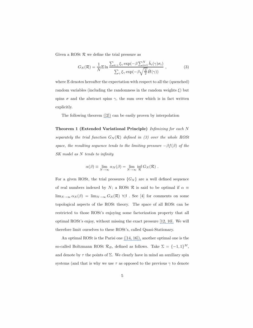
Given a ROSt R we define the trial pressure as

GN (R) =1

NE ln

∑

σ,γ ξγ exp(−β∑Ni=1

hi(γ)σi)∑

γ ξγ exp(−β√

N2H(γ))

, (3)

where E denotes hereafter the expectation with respect to all the (quenched)

random variables (including the randomness in the random weights ξ) but

spins σ and the abstract spins γ, the sum over which is in fact written

explicitly.

The following theorem ([2]) can be easily proven by interpolation

Theorem 1 (Extended Variational Principle) Infimizing for each N

separately the trial function GN (R) defined in (3) over the whole ROSt

space, the resulting sequence tends to the limiting pressure −βf(β) of the

SK model as N tends to infinity

α(β) ≡ limN→∞

αN (β) = limN→∞

infRGN (R) .

For a given ROSt, the trial pressures GN are a well defined sequence

of real numbers indexed by N ; a ROSt R is said to be optimal if α ≡

limN→∞ αN (β) = limN→∞GN (R) ∀β . See [4] for comments on some

topological aspects of the ROSt theory. The space of all ROSt can be

restricted to those ROSt’s enjoying some factorization property that all

optimal ROSt’s enjoy, without missing the exact pressure [12, 10]. We will

therefore limit ourselves to these ROSt’s, called Quasi-Stationary.

An optimal ROSt is the Parisi one ([14, 16]), another optimal one is the

so-called Boltzmann ROSt RB , defined as follows. Take Σ = −1, 1M ,

and denote by τ the points of Σ. We clearly have in mind an auxiliary spin

systems (and that is why we use τ as opposed to the previous γ to denote

5

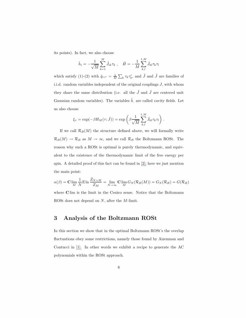
its points). In fact, we also choose

hi = − 1√M

M∑

k=1

Jikτk , H = − 1

M

1,M∑

k,l

Jklτkτl

which satisfy (1)-(2) with qττ ′ = 1

M

∑

k τkτ′k, and J and J are families of

i.i.d. random variables independent of the original couplings J , with whom

they share the same distribution (i.e. all the J and J are centered unit

Gaussian random variables). The variables h. are called cavity fields. Let

us also choose

ξτ = exp(−βHM (τ ; J)) = exp

(

β1√M

1,M∑

k,l

Jklτkτl

)

.

If we call RB(M) the structure defined above, we will formally write

RB(M) → RB as M → ∞, and we call RB the Boltzmann ROSt. The

reason why such a ROSt is optimal is purely thermodynamic, and equiv-

alent to the existence of the thermodynamic limit of the free energy per

spin. A detailed proof of this fact can be found in [2]; here we just mention

the main point:

α(β) = C limM

1

NE ln

ZN+M

ZM

= limN→∞

C limMGN (RB(M)) = GN (RB) = G(RB)

where C lim is the limit in the Cesaro sense. Notice that the Boltzmann

ROSt does not depend on N , after the M -limit.

3 Analysis of the Boltzmann ROSt

In this section we show that in the optimal Boltzmann ROSt’s the overlap

fluctuations obey some restrictions, namely those found by Aizenman and

Contucci in [1]. In other words we exhibit a recipe to generate the AC

polynomials within the ROSt approach.

6

3.1 the internal energy term

Let us focus on the denominator of the trial pressure G(RB), defined in

(3), computed at the Boltzmann ROSt RB , defined in the previous sec-

tion. Let us normalize this quantity by dividing by ZN and weight H with

an independent variable β′ as opposed to β, which appears in the Boltz-

mannfaktor ξτ . As in the Boltzmann structure we have actual spins (τ)

and we do not use the spins σ here, we will still use ω (or Ω) to denote

the Boltzmann-Gibbs (replica) measure (at inverse temperature β) in the

space Σ = −1, 1M . Moreover, we will use the notation 〈·〉 = EΩ(·) and,

if present, a subscript β recalls that the Boltzmannfaktor in Ω has inverse

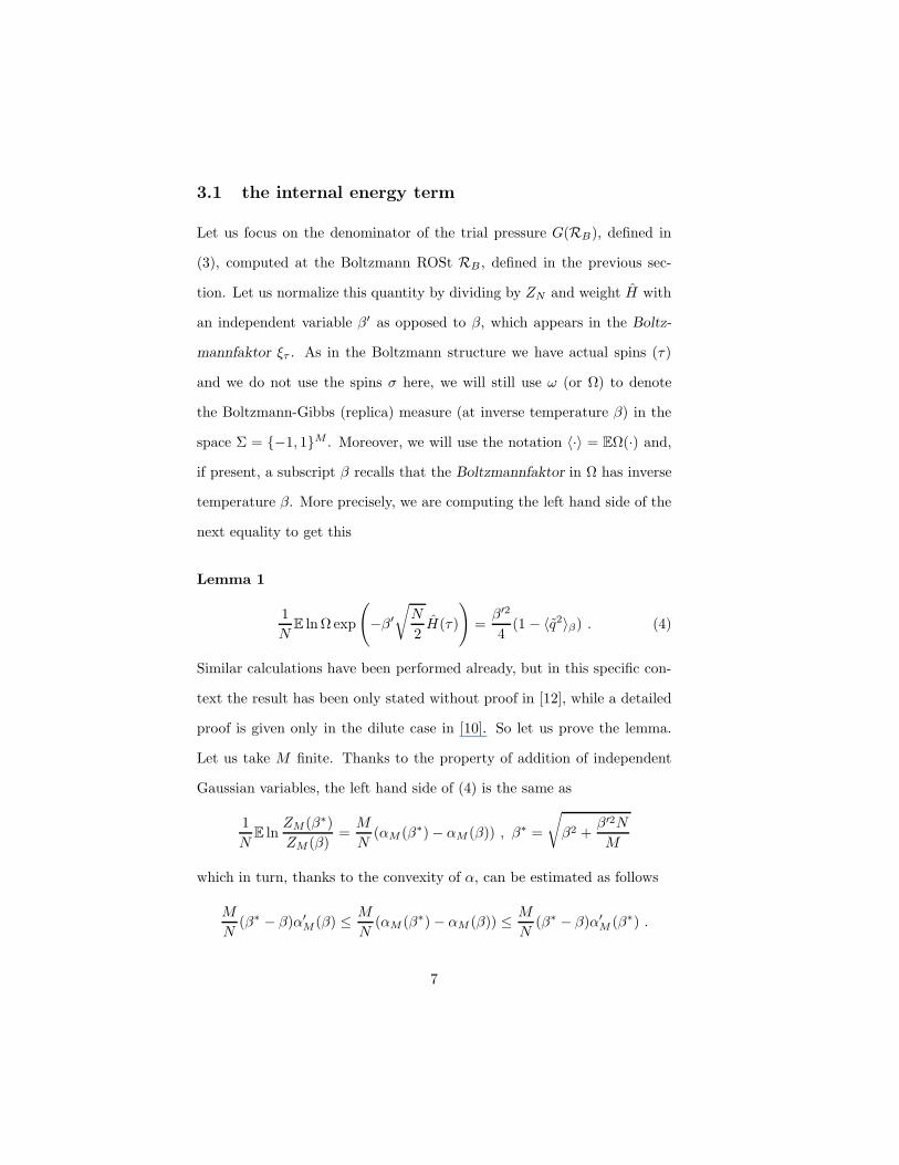
temperature β. More precisely, we are computing the left hand side of the

next equality to get this

Lemma 1

1

NE ln Ω exp

(

−β′

√

N

2H(τ)

)

=β′2

4(1 − 〈q2〉β) . (4)

Similar calculations have been performed already, but in this specific con-

text the result has been only stated without proof in [12], while a detailed

proof is given only in the dilute case in [10]. So let us prove the lemma.

Let us take M finite. Thanks to the property of addition of independent

Gaussian variables, the left hand side of (4) is the same as

1

NE ln

ZM (β∗)

ZM (β)=M

N(αM (β∗) − αM (β)) , β∗ =

√

β2 +β′2N

M

which in turn, thanks to the convexity of α, can be estimated as follows

M

N(β∗ − β)α′

M (β) ≤ M

N(αM (β∗) − αM (β)) ≤ M

N(β∗ − β)α′

M (β∗) .

7

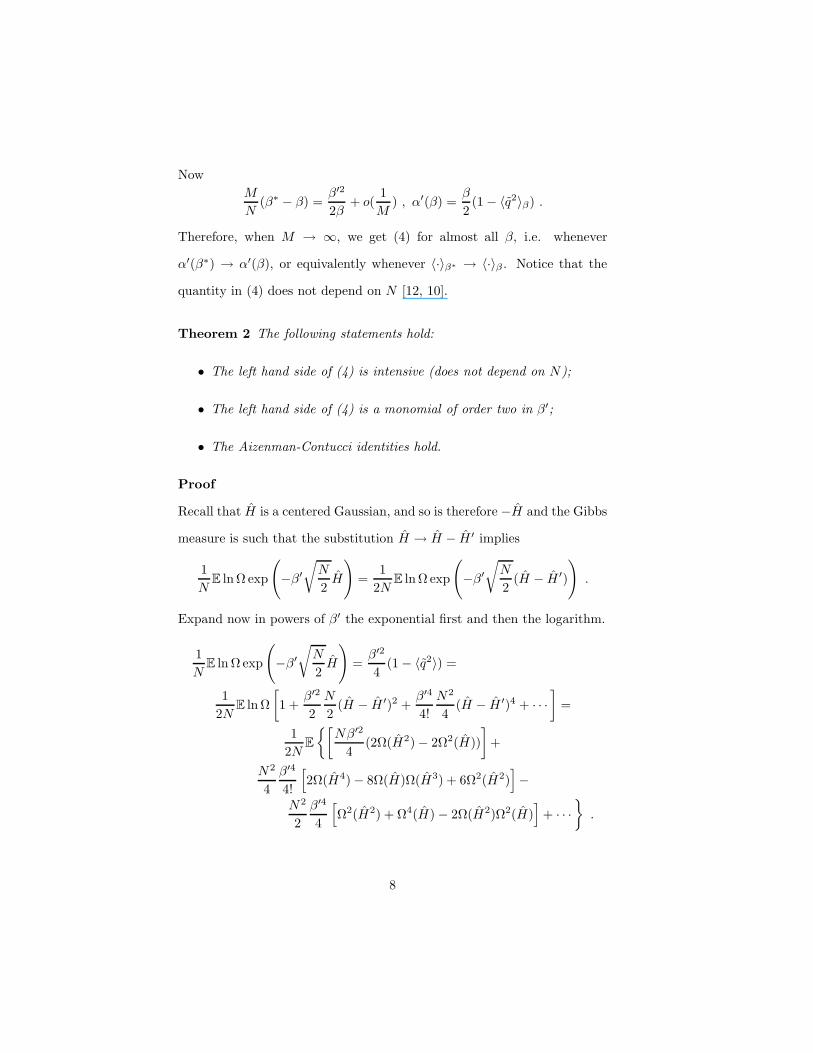
Now

M

N(β∗ − β) =

β′2

2β+ o(

1

M) , α′(β) =

β

2(1 − 〈q2〉β) .

Therefore, when M → ∞, we get (4) for almost all β, i.e. whenever

α′(β∗) → α′(β), or equivalently whenever 〈·〉β∗ → 〈·〉β . Notice that the

quantity in (4) does not depend on N [12, 10].

Theorem 2 The following statements hold:

• The left hand side of (4) is intensive (does not depend on N);

• The left hand side of (4) is a monomial of order two in β′;

• The Aizenman-Contucci identities hold.

Proof

Recall that H is a centered Gaussian, and so is therefore −H and the Gibbs

measure is such that the substitution H → H − H ′ implies

1

NE ln Ω exp

(

−β′

√

N

2H

)

=1

2NE ln Ω exp

(

−β′

√

N

2(H − H ′)

)

.

Expand now in powers of β′ the exponential first and then the logarithm.

1

NE ln Ω exp

(

−β′

√

N

2H

)

=β′2

4(1 − 〈q2〉) =

1

2NE ln Ω

[

1 +β′2

2

N

2(H − H ′)2 +

β′4

4!

N2

4(H − H ′)4 + · · ·

]

=

1

2NE

[

Nβ′2

4(2Ω(H2) − 2Ω2(H))

]

+

N2

4

β′4

4!

[

2Ω(H4) − 8Ω(H)Ω(H3) + 6Ω2(H2)]

−

N2

2

β′4

4

[

Ω2(H2) + Ω4(H) − 2Ω(H2)Ω2(H)]

+ · · ·

.

8

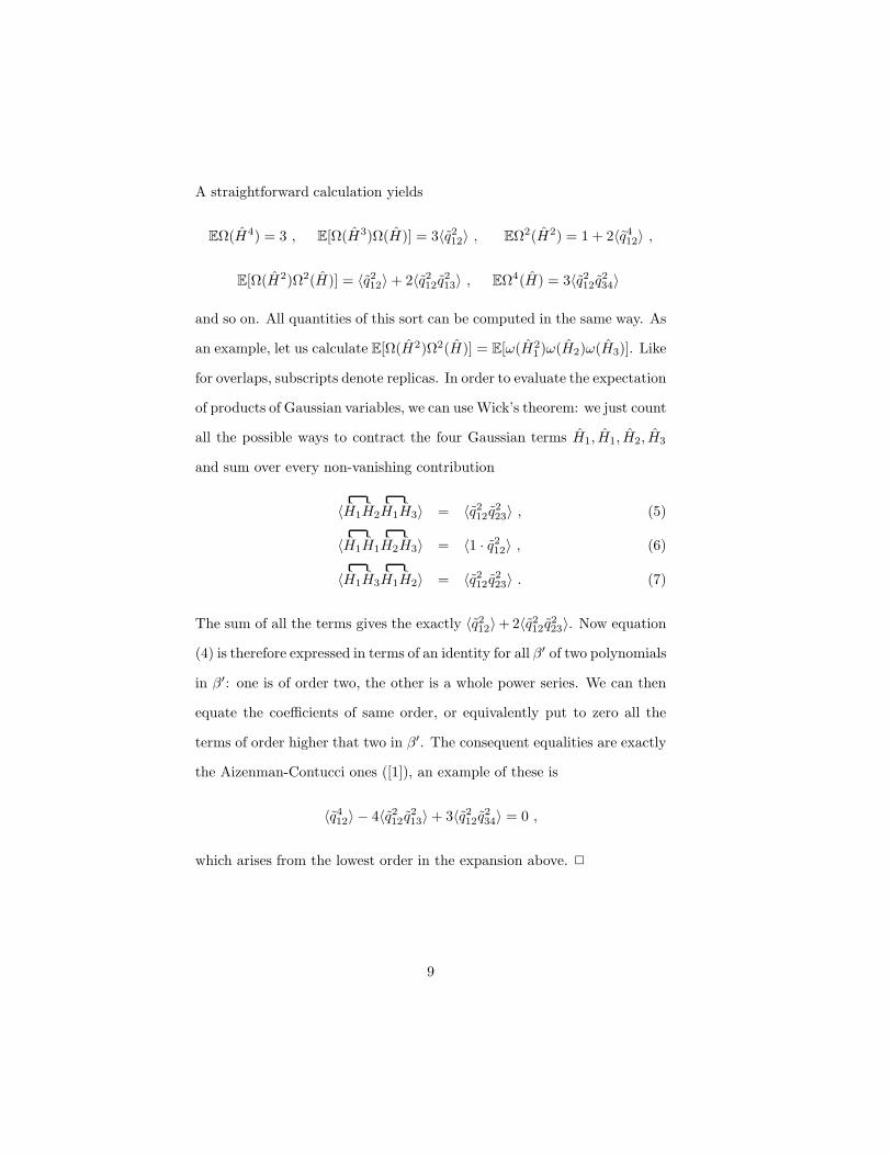
A straightforward calculation yields

EΩ(H4) = 3 , E[Ω(H3)Ω(H)] = 3〈q212〉 , EΩ2(H2) = 1 + 2〈q412〉 ,

E[Ω(H2)Ω2(H)] = 〈q212〉 + 2〈q212q213〉 , EΩ4(H) = 3〈q212q234〉

and so on. All quantities of this sort can be computed in the same way. As

an example, let us calculate E[Ω(H2)Ω2(H)] = E[ω(H21 )ω(H2)ω(H3)]. Like

for overlaps, subscripts denote replicas. In order to evaluate the expectation

of products of Gaussian variables, we can use Wick’s theorem: we just count

all the possible ways to contract the four Gaussian terms H1, H1, H2, H3

and sum over every non-vanishing contribution

〈H1H2H1H3〉 = 〈q212q223〉 , (5)

〈H1H1H2H3〉 = 〈1 · q212〉 , (6)

〈H1H3H1H2〉 = 〈q212q223〉 . (7)

The sum of all the terms gives the exactly 〈q212〉+ 2〈q212q223〉. Now equation

(4) is therefore expressed in terms of an identity for all β′ of two polynomials

in β′: one is of order two, the other is a whole power series. We can then

equate the coefficients of same order, or equivalently put to zero all the

terms of order higher that two in β′. The consequent equalities are exactly

the Aizenman-Contucci ones ([1]), an example of these is

〈q412〉 − 4〈q212q213〉 + 3〈q212q234〉 = 0 ,

which arises from the lowest order in the expansion above.

9

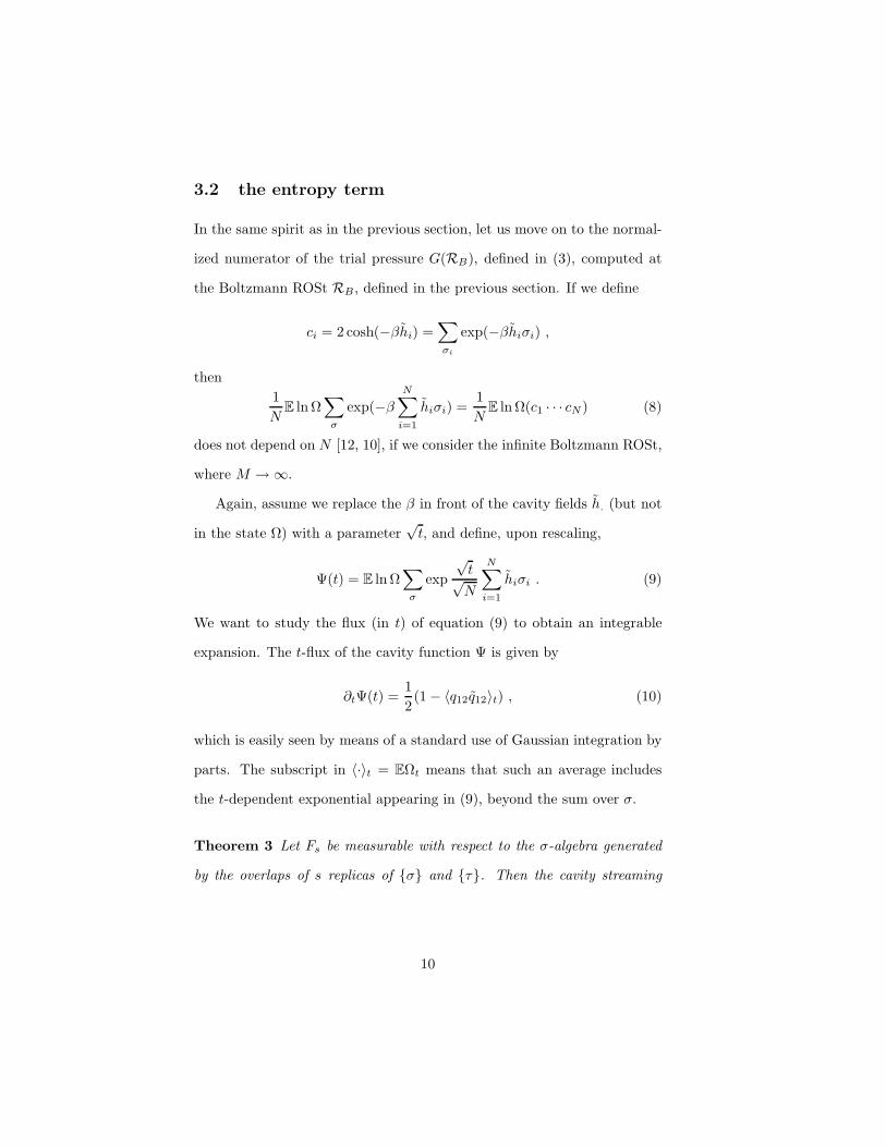
3.2 the entropy term

In the same spirit as in the previous section, let us move on to the normal-

ized numerator of the trial pressure G(RB), defined in (3), computed at

the Boltzmann ROSt RB , defined in the previous section. If we define

ci = 2 cosh(−βhi) =∑

σi

exp(−βhiσi) ,

then

1

NE ln Ω

∑

σ

exp(−βN∑

i=1

hiσi) =1

NE ln Ω(c1 · · · cN ) (8)

does not depend on N [12, 10], if we consider the infinite Boltzmann ROSt,

where M → ∞.

Again, assume we replace the β in front of the cavity fields h. (but not

in the state Ω) with a parameter√t, and define, upon rescaling,

Ψ(t) = E ln Ω∑

σ

exp

√t√N

N∑

i=1

hiσi . (9)

We want to study the flux (in t) of equation (9) to obtain an integrable

expansion. The t-flux of the cavity function Ψ is given by

∂tΨ(t) =1

2(1 − 〈q12q12〉t) , (10)

which is easily seen by means of a standard use of Gaussian integration by

parts. The subscript in 〈·〉t = EΩt means that such an average includes

the t-dependent exponential appearing in (9), beyond the sum over σ.

Theorem 3 Let Fs be measurable with respect to the σ-algebra generated

by the overlaps of s replicas of σ and τ. Then the cavity streaming

10

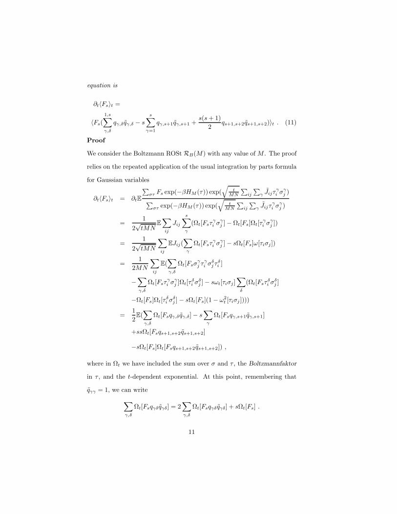
equation is

∂t〈Fs〉t =

〈Fs(

1,s∑

γ,δ

qγ,δqγ,δ − s

s∑

γ=1

qγ,s+1qγ,s+1 +s(s+ 1)

2qs+1,s+2qs+1,s+2)〉t . (11)

Proof

We consider the Boltzmann ROSt RB(M) with any value of M . The proof

relies on the repeated application of the usual integration by parts formula

for Gaussian variables

∂t〈Fs〉t = ∂tE

∑

στ Fs exp(−βHM (τ)) exp(√

tMN

∑

ij

∑

γ Jijτγi σ

γj )

∑

στ exp(−βHM (τ)) exp(√

tMN

∑

ij

∑

γ Jijτγi σ

γj )

=1

2√tMN

E

∑

ij

Jij

s∑

γ

(Ωt[Fsτγi σ

γj ] − Ωt[Fs]Ωt[τ

γi σ

γj ])

=1

2√tMN

∑

ij

EJij(∑

γ

Ωt[Fsτγi σ

γj ] − sΩt[Fs]ω[τiσj ])

=1

2MN

∑

ij

E(∑

γ,δ

Ωt[Fsσγj τ

γi σ

δj τ

δi ]

−∑

γ,δ

Ωt[Fsτγi σ

γj ]Ωt[τ

δi σ

δj ] − sωt[τiσj ]

∑

δ

(Ωt[Fsτδi σ

δj ]

−Ωt[Fs]Ωt[τδi σ

δj ] − sΩt[Fs](1 − ω2

t [τiσj ])))

=1

2E(∑

γ,δ

Ωt[Fsqγ,δ qγ,δ] − s∑

γ

Ωt[Fsqγ,s+1qγ,s+1]

+ssΩt[Fsqs+1,s+2qs+1,s+2]

−sΩt[Fs]Ωt[Fsqs+1,s+2qs+1,s+2]) ,

where in Ωt we have included the sum over σ and τ , the Boltzmannfaktor

in τ , and the t-dependent exponential. At this point, remembering that

qγγ = 1, we can write

∑

γ,δ

Ωt[Fsqγδ qγδ] = 2∑

γ,δ

Ωt[Fsqγδ qγδ] + sΩt[Fs] .

11

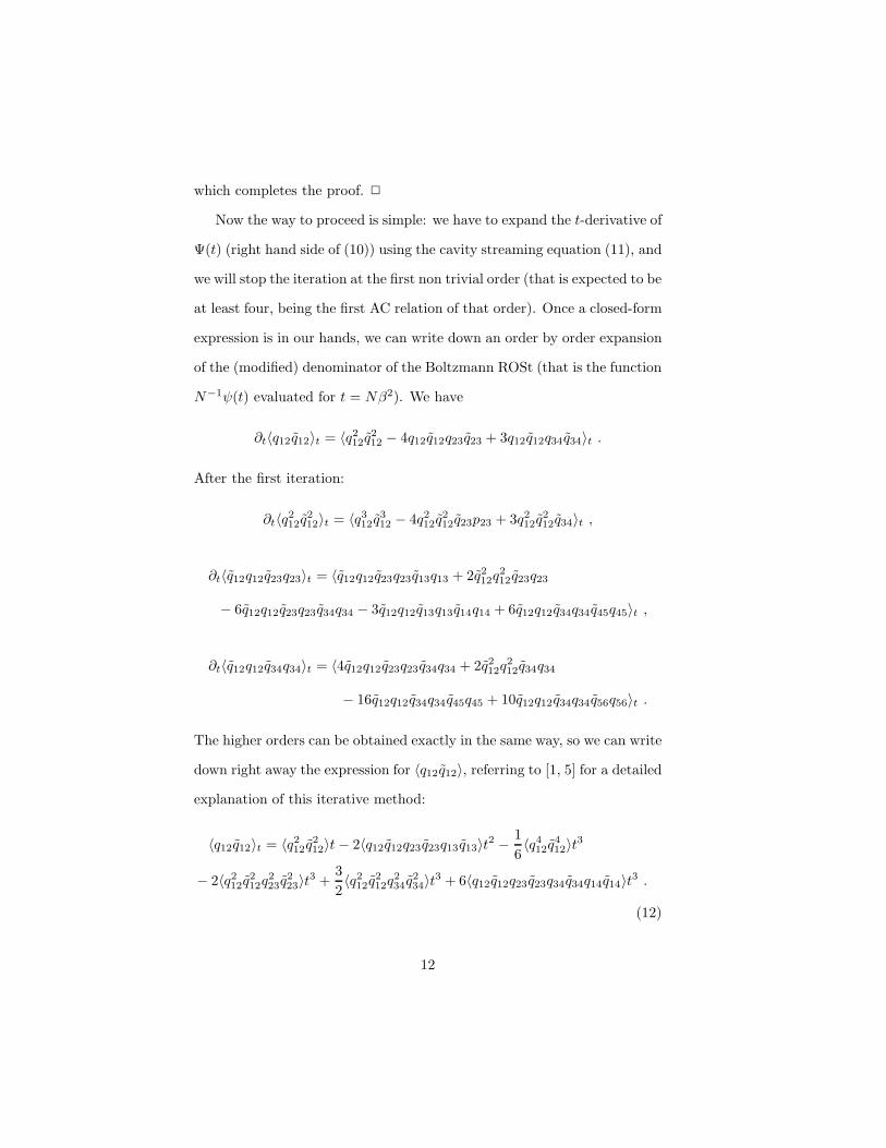
which completes the proof.

Now the way to proceed is simple: we have to expand the t-derivative of

Ψ(t) (right hand side of (10)) using the cavity streaming equation (11), and

we will stop the iteration at the first non trivial order (that is expected to be

at least four, being the first AC relation of that order). Once a closed-form

expression is in our hands, we can write down an order by order expansion

of the (modified) denominator of the Boltzmann ROSt (that is the function

N−1ψ(t) evaluated for t = Nβ2). We have

∂t〈q12q12〉t = 〈q212q212 − 4q12q12q23q23 + 3q12q12q34q34〉t .

After the first iteration:

∂t〈q212q212〉t = 〈q312q312 − 4q212q212q23p23 + 3q212q

212q34〉t ,

∂t〈q12q12q23q23〉t = 〈q12q12q23q23q13q13 + 2q212q212q23q23

− 6q12q12q23q23q34q34 − 3q12q12q13q13q14q14 + 6q12q12q34q34q45q45〉t ,

∂t〈q12q12q34q34〉t = 〈4q12q12q23q23q34q34 + 2q212q212q34q34

− 16q12q12q34q34q45q45 + 10q12q12q34q34q56q56〉t .

The higher orders can be obtained exactly in the same way, so we can write

down right away the expression for 〈q12q12〉, referring to [1, 5] for a detailed

explanation of this iterative method:

〈q12q12〉t = 〈q212q212〉t− 2〈q12q12q23q23q13q13〉t2 −1

6〈q412q412〉t3

− 2〈q212q212q223q223〉t3 +3

2〈q212q212q234q234〉t3 + 6〈q12q12q23q23q34q34q14q14〉t3 .

(12)

12

Notice that the averages no longer depend on t. In this expansion we

considered both q-overlaps and q-overlaps, but as the sum over the spins σ

can be performed explicitly, we can obtain an explicit expression at least

for the q-overlaps, and get

〈q212〉 =1

N2E

∑

ij

ω2(σiσj) =1

N,

〈q12q23q31〉 =1

N3E

∑

ijk

ω(σiσj)ω(σjσk)ω(σkσi) =1

N2,

〈q212q234〉 =1

N4E

∑

ijkl

ω2(σiσj)ω2(σkσl) =

1

N2,

〈q12q23q34q14〉 =1

N4E

∑

ijkl

ω(σiσj)ω(σjσk)ω(σkσl)ω(σlσi) =1

N3,

〈q412〉 =1

N4E

∑

ijkl

ω(σiσjσkσl)ω(σiσjσkσl) =3(N − 1)

N3+

1

N3,

〈q212q223〉 =1

N4E

∑

ijkl

ω(σiσj)ω(σiσjσkσl)ω(σiσj) =1

N2.

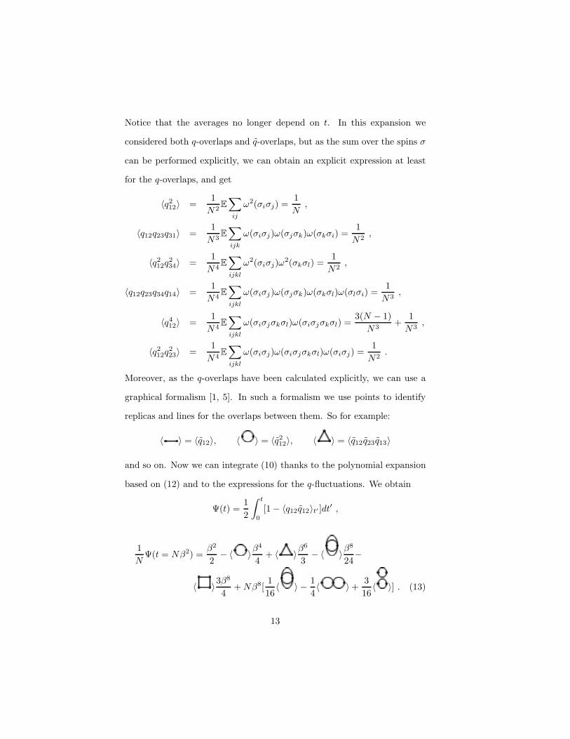
Moreover, as the q-overlaps have been calculated explicitly, we can use a

graphical formalism [1, 5]. In such a formalism we use points to identify

replicas and lines for the overlaps between them. So for example:

〈 〉 = 〈q12〉, 〈 〉 = 〈q212〉, 〈 〉 = 〈q12q23q13〉

and so on. Now we can integrate (10) thanks to the polynomial expansion

based on (12) and to the expressions for the q-fluctuations. We obtain

Ψ(t) =1

2

∫ t

0

[1 − 〈q12q12〉t′ ]dt′ ,

1

NΨ(t = Nβ2) =

β2

2− 〈 〉β

4

4+ 〈 〉β

6

3− 〈 〉β

8

24−

〈 〉3β8

4+Nβ8[

1

16〈 〉 − 1

4〈 〉 +

3

16〈 〉] . (13)

13

This expression, though truncated at this low order, already looks pretty

much alike the expansion found using the internal energy part of the Boltz-

mann pressure.

We stress however two important features of expression (13). The first is

that within this approach we do not have problems concerning the Replica

Simmetry Anzatz (RS) [14], and this can be seen by the proliferating of the

overalaps fluctuations, via which we expand the entropy (a RS theory does

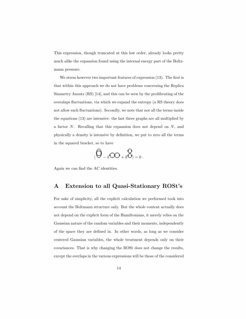
not allow such fluctuations). Secondly, we note that not all the terms inside

the equations (13) are intensive: the last three graphs are all multiplied by

a factor N . Recalling that this expansion does not depend on N , and

physically a density is intensive by definition, we put to zero all the terms

in the squared bracket, so to have

〈 − 4 + 3 〉 = 0 .

Again we can find the AC identities.

A Extension to all Quasi-Stationary ROSt’s

For sake of simplicity, all the explicit calculation we performed took into

account the Boltmann structure only. But the whole content actually does

not depend on the explicit form of the Hamiltonians, it merely relies on the

Gaussian nature of the random variables and their moments, independently

of the space they are defined in. In other words, as long as we consider

centered Gaussian variables, the whole treatment depends only on their

covariances. That is why changing the ROSt does not change the results,

except the overlaps in the various expressions will be those of the considered

14

ROSt (e.g. the ultrametric Parisi trial overlaps), provided some properties

are preserved (Quasi-Stationarity).

Let us focus for instance on the internal energy part, which is sim-

pler, and see that the results of subsection 3.1 are the same in any Quasi-

Stationary ROSt. First of all, notice that the proof of Theorem 2 never

makes use of the explicit form of the Hamiltonians and therefore (5)-(6)-

(7) stay identical, as they are determined purely by the covariances of the

Hamiltonians. The same clearly holds for all the other terms not explicitly

considered in the example.

So the validity of the results coincides with the validity of Lemma 1.

The ROSt’s for which such a lemma holds are called Quasi-Stationary (see

[3, 4]), in this case with respect to the Cavity Step (see [12, 3]). Notice

that the left hand side of (4) is zero for β′ = 0 independently of the par-

ticular ROSt. Hence by the fundamental theorem of calculus the same left

hand side coincides with the integral from zero to β′ of its derivative (with

respect to β′). But the form of such a derivative is just determined by the

covariance of H (this is at the heart of [2]), which is always defined to be

an overlap. Therefore a simple Gaussian integration by parts, as illustrated

in [2], leads to the right hand side of (4). These are the intuitive reasons

that heuristically explain why both the explicit calculation in Lemma 1 and

the expansion of Theorem 2 are the same in any Quasi-Stationary ROSt,

and so are the AC polynomials, no matter what the overlap looks like in

a generic abstract space. So AC polynomials hold in any Quasi-Stationary

ROSt, non-optimal too, but if the chosen ROSt is not optimal there will

be no overlap locking and the trial overlap will have very little to share

15

with the true ones of the model. Moreover (4) will not in general provide

the internal energy of the model (but this can be the case in some optimal

ROSt too, like the Parisi one!).

Conclusions and Outlook

We have shown how some constraints on the distribution of the overlap nat-

urally arise within the Random Overlap Structure approach. As our anal-

ysis of the Boltzmann ROSt is similar to the study of stochastic stability it

is not surprising that the constraints coincide with the Aizenman-Contucci

identities. In the ROSt context, such identities are easily connected with

the existence of the thermodynamic limit of the free energy density (which

is equivalent to the optimality of the Boltzmann ROSt) and with the phys-

ical fact that the internal energy is intensive. We also showed that, as

expected, the entropy part of the free energy yields the same constraints

as the other part (i.e. the internal energy).

The hope for the near future is that the ROSt approach will lead even-

tually to a good understanding of the pure states and the phase transitions

of the model. A first step has been taken in [12], and our present results can

be considered as a second step in this direction. (Other more interesting

results regarding the phase transition at β = 1 can also be obtained with

the same techniques employed here, including the graphical representation

[6].) A further step should bring the Ghirlanda-Guerra identities, and then

hopefully a proof of ultrametricity.

16

Acknowledgment

The authors warmly thank Francesco Guerra and Pierluigi Contucci for a

precious scientific and personal support, and sincerely thank Peter Sollich

for useful discussions and much advice. A grateful appreciation is owed to

Louis-Pierre Arguin for pointing out a weak point in a previous version of

the paper and for very fruitful conversations.

References

[1] M. Aizenman, P. Contucci, On the stability of the quenched state in

mean field spin glass models, J. Stat. Phys. 92, 765-783 (1998).

[2] M. Aizenman, R. Sims, S. L. Starr, An Extended Variational Principle

for the SK Spin-Glass Model, Phys. Rev. B, 68, 214403 (2003).

[3] M. Aizenman, R. Sims, S. L. Starr, Mean-Field Spin Glass models from

the Cavity-ROSt Perspective, ArXiv: math-ph/0607060.

[4] L.-P. Arguin, pin Glass Computations and Ruelle’s Probability Cas-

cades, ArXiv: math-ph/0608045, to appear in J. Stat. Phys..

[5] A. Barra, Irreducible free energy expansion for mean field spin glass

model, J. Stat. Phys. (2006) DOI: 10.1007/s10955-005-9006-6.

[6] A. Agostini, A. Barra, L. De Sanctis, in preparation.

[7] A. Bovier, Statistical Mechanics of Disordered Systems, A mathematical

perspective, Cambridge University Press (2006).

17

[8] P. Contucci, C. Giardina, Spin-Glass Stochastic Stability: a Rigorous

Proof, ArXiv: math-ph/0408002.

[9] P. Contucci, C. Giardina, The Ghirlanda-Guerra identities, ArXiv:

math-ph/0505055v1.

[10] L. De Sanctis, Random Multi-Overlap Structures and Cavity Fields in

Diluted Spin Glasses, J. Stat. Phys. 117 785-799 (2004).

[11] S. Ghirlanda, F. Guerra, General properties of overlap distributions in

disordered spin systems. Towards Parisi ultrametricity, J. Phys. A, 31

9149-9155 (1998).

[12] F. Guerra, About the Cavity Fields in Mean Field Spin Glass Models,

ArXiv: cond-mat/0307673.

[13] F. Guerra, Broken Replica Symmetry Bounds in the Mean Field Spin

Glass Model, Commun, Math. Phys. 233:1 1-12 (2003).

[14] M. Mezard, G. Parisi and M. A. Virasoro, Spin glass theory and be-

yond, World Scientific, Singapore (1987).

[15] G. Parisi, On the probabilistic formulation of the replica approach to

spin glasses, Int. Jou. Mod. Phys. B 18, 733-744, (2004).

[16] M. Talagrand, The Parisi Formula, Annals of Mathematics, 163, 221

(2006).

[17] M. Talagrand, Spin glasses: a challenge for mathematicians. Cavity

and Mean field models, Springer Verlag (2003).

18