Overland water and salt flows in a set of rice paddies

a g r i c u l t u r a l w a t e r m a n a g e m e n t 9 5 ( 2 0 0 8 ) 6 4 5 – 6 5 8

avai lab le at www.sc iencedi rec t .com

journal homepage: www.e lsev ier .com/ locate /agwat

Overland water and salt flows in a set of rice paddies

E. Playan a,*, O. Perez-Coveta a, A. Martınez-Cob a, J. Herrero b,P. Garcıa-Navarro c, B. Latorre c, P. Brufau c, J. Garces c

aDepartamento Suelo y Agua, Estacion Experimental de Aula Dei, CSIC, P.O. Box 202, 50080 Zaragoza, SpainbUnidad de Suelos y Riegos (Associated Unit to Estacion Experimental de Aula Dei, CSIC), CITA, P.O Box 727, 50080 Zaragoza, Spainc Area de Mecanica de Fluidos, CPS, Universidad de Zaragoza, Marıa de Luna 3, 50018 Zaragoza, Spain

a r t i c l e i n f o

Article history:

Received 5 October 2007

Accepted 15 January 2008

Published on line 12 March 2008

Keywords:

Ebro

Aragon

Spain

Efficiency

Simulation

Saline-sodic

Salinity

Infiltration

Runoff

Percolation

a b s t r a c t

Cultivation of paddy rice in semiarid areas of the world faces problems related to water

scarcity. This paper aims at characterizing water use in a set of paddies located in the central

Ebro basin of Spain using experimentation and computer simulation. A commercial field

with six interconnected paddies, with a total area of 5.31 ha, was instrumented to measure

discharge and water quality at the inflow and at the runoff outlet. The soil was classified as a

Typic Calcixerept, and was characterized by a mild salinity (2.5 dS m�1) and an infiltration rate

of 5.8 mm day�1. The evolution of flow depth at all paddies was recorded. Data from the 2002

rice-growing season was elaborated using a mass balance approach to estimate the infil-

tration rate and the evolution of discharge between paddies. Seasonal crop evapotranspira-

tion, estimated with the surface renewal method, was 731 mm (5.1 mm day�1), very similar

to that of other summer cereals grown in the area, like corn. The irrigation input was

1874 mm, deep percolation was 830 mm and surface runoff was 372 mm. Irrigation effi-

ciency was estimated as 41%. The quality of surface runoff water was slightly degraded due

to evapoconcentration and to the contact with the soil. During the period 2001–2003, the

electrical conductivity of surface runoff water was 54% higher than that of irrigation water.

However, the runoff water was suitable for irrigation. A mechanistic mass balance model of

inter-paddy water flow permitted to conclude that improvements in irrigation efficiency

cannot be easily obtained in the experimental conditions. Since deep percolation losses

more than double surface runoff losses, a reduction in irrigation discharge would not have

much room for efficiency improvement. Simulations also showed that rice irrigation

performance was not negatively affected by the fluctuating inflow hydrograph. These

hydrographs are typical of turnouts located at the tail end of tertiary irrigation ditches.

In fact, these are the sites where rice has been historically cultivated in the study area, since

local soils are often saline-sodic and can only grow paddy rice taking advantage of the low

salinity of the irrigation water. The low infiltration rate characteristic of these saline-sodic

soils (an experimental value of 3.2 mm day�1 was obtained) combined with a reduced

irrigation discharge resulted in a simulated irrigation efficiency of 60%. Paddy rice irrigation

efficiency can attain reasonable values in the local saline-sodic soils, where the infiltration

rate is clearly smaller than the average daily rice evapotranspiration.

# 2008 Elsevier B.V. All rights reserved.

* Corresponding author. Tel.: +34 976 716 087; fax: +34 976 716 145.E-mail address: [email protected] (E. Playan).

0378-3774/$ – see front matter # 2008 Elsevier B.V. All rights reservedoi:10.1016/j.agwat.2008.01.012

d.

mailto:[email protected]

http://dx.doi.org/10.1016/j.agwat.2008.01.012


1. Introduction

In water-scarce regions of the world rice cultivation is often

criticised for using too much water. Tuong and Bhuiyan (1999)

summarised the results of a number of researchers in which

rice irrigation efficiency fluctuated between 22 and 61%. These

results are in reasonable agreement with those of Clemmens

and Dedrick (1994), who presented a pessimistic and an

optimistic estimation of paddy rice efficiency, with respective

values of 40 and 60%. According to these figures, it is clear that

paddy rice ranks very low in the comparison of irrigated

agricultural systems based on irrigation efficiency.

A number of authors (Keller et al., 1996; Perry, 1999) have

emphasized the hydrologic implications of irrigation effi-

ciency, particularly in what refers to upscaling. A common

conclusion of these works is that low values of on-farm

irrigation efficiency (Burt et al., 1997) may not be harmful to

regional water availability if the quality and location of the

return flows permit to reuse them. In fact, water reuse is a very

common feature of rice-growing areas, in which water flows

from paddy to paddy following intricate paths. Recently,

Hafeez et al. (2007) presented data on an irrigated rice project

in the Philippines. Water reuse at various levels resulted in a

regional irrigation efficiency of 71%. The authors believed that

achieving 80% efficiency would not require major improve-

ments in irrigation management and structures. Similar

conclusions can be drawn in the central Ebro basin of Spain

when taking into account non-point source water reuse in the

Flumen irrigation district (Nogues and Herrero, 2003). These

regional figures should alleviate social pressure on rice

cultivation in areas where return flows are reused.

The reduction of on-farm water use presents advantages

over return flow reuse. These are related to the conservation of

water quantity (keeping irrigation water at the system source;

controlling water table rise) and quality conservation (avoid-

ing the pollution present in runoff and percolation water). This

is the reason why a number of techniques have been proposed

to improve on-farm rice irrigation efficiency, such as soil

puddling (Kukal and Aggarwal, 2002), intermittent ponding

(Belder et al., 2004), soil suitability assessment (Beecher et al.,

2002) and nonsubmerged sprinkler irrigation (McCauley, 1990).

The central Ebro Valley of Spain has an irrigated area of

about half a million hectares.The area cropped to rice fluctuates

every year, but rarely exceeds 20,000 ha. Rice is not particularly

important in the region from a water use perspective, but it

Table 1 – Main characteristics of the paddies: area (m2), averagedeviation of soil surface elevation (SDe, m), number of EMI re

Paddy # Area (m2) Elevation (m) SDe (m) EMI readin

1 7,973 4.26 0.021 17

2 10,004 2.57 0.010 20

3 5,844 1.62 0.019 10

4 7,188 0.99 0.020 15

5 8,240 0.26 0.019 21

6 13,866 0.00 0.014 18

All 53,115 � 0.017 101

occupies its own niche: it is the only cropping alternative for

saline-sodic soils. The vertical saturated hydraulic conductivity

of these soils is usually very low, due to: (1) a degraded structure;

(2) the frequent alternating millimetric layers of silt and sodic

clay of the underlying Holocene sediments; and (3) soil tillage,

puddling with the rice straw to produce an impervious soil pan.

As a consequence, rice irrigation can attain reasonable

efficiencies. In these crop conditions, soil salinity does not

pose a limitation to rice growth and yield due to the permanent

flooding with fresh water. Saline-sodic soils are often located in

poorly drained, low geomorphic positions. Rice is cultivated

every year in these soils. In the years when rice is particularly

profitable, the crop can also be found in non saline-sodic soils

occupying higher geomorphic positions. Rice farms in the area

often occupy between 3 and 10 ha, and are typically divided into

a number of paddies, with 0.5–2 ha each. The set of paddies has

a canal turnout and a runoff disposal point, and water

continuously flows between paddies during the crop season.

Rainfall usually represents a small fraction of the seasonal

water input.

The objectives of this paper are: (1) to assess water use in a

set of rice paddies in the central Ebro basin, estimating all terms

of the hydrologic balance as well as irrigation performance; (2)

to evaluate the quality of irrigation and surface runoff waters;

(3) to assess the influence of soil infiltration on irrigation

performance; and (4) to identify better performing irrigation

management techniques, capable of reducing surface runoff.

2. Materials and methods

2.1. The experimental field

A commercial rice field located in Albero Bajo (Huesca, Ebro

valley, Spain) was evaluated in 2002 for irrigation performance

and during 2001, 2002 and 2003 for irrigation and runoff water

quality. The coordinates of the field are 4185905300N and

082403400W. The total field area was 5.31 ha, divided into six

paddies with areas ranging between 0.58 and 1.39 ha (Table 1,

Fig. 1). A topographic survey revealed that the difference in

elevation between the highest and the lowest paddies was

4.26 m. The standard deviation of soil surface elevation

(Playan et al., 1996) for each paddy ranged between 0.010

and 0.021 m, indicating that the field had been laser-levelled in

recent years. Rice was grown annually in the field since 1996,

soil surface elevation (m, referenced to paddy 6), standardadings, and statistics of the ECe 0–50 cm estimates

gs ECe 0–50 cm estimates

Mean(dS m�1)

Median(dS m�1)

Min.(dS m�1)

Max.(dS m�1)

C.V.(%)

1.53 1.43 1.07 2.09 22.2

1.32 1.26 0.92 2.05 24.2

1.44 1.43 1.05 1.71 16.0

1.86 1.69 1.15 3.40 37.1

4.68 4.31 2.49 9.86 46.2

3.31 2.69 2.10 8.56 48.6

2.50 1.96 0.92 9.86 71.6

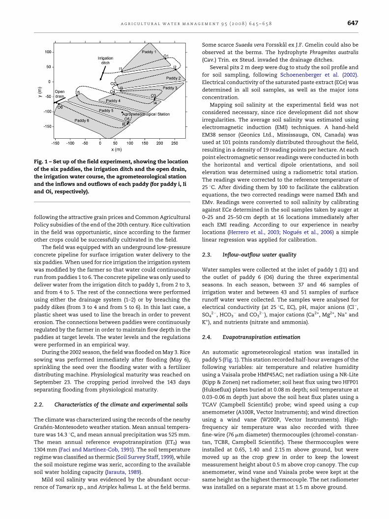
Fig. 1 – Set up of the field experiment, showing the location

of the six paddies, the irrigation ditch and the open drain,

the irrigation water course, the agrometeorological station

and the inflows and outflows of each paddy (for paddy i, Ii

and Oi, respectively).

a g r i c u l t u r a l w a t e r m a n a g e m e n t 9 5 ( 2 0 0 8 ) 6 4 5 – 6 5 8 647

following the attractive grain prices and Common Agricultural

Policy subsidies of the end of the 20th century. Rice cultivation

in the field was opportunistic, since according to the farmer

other crops could be successfully cultivated in the field.

The field was equipped with an underground low-pressure

concrete pipeline for surface irrigation water delivery to the

six paddies. When used for rice irrigation the irrigation system

was modified by the farmer so that water could continuously

run from paddies 1 to 6. The concrete pipeline was only used to

deliver water from the irrigation ditch to paddy 1, from 2 to 3,

and from 4 to 5. The rest of the connections were performed

using either the drainage system (1–2) or by breaching the

paddy dikes (from 3 to 4 and from 5 to 6). In this last case, a

plastic sheet was used to line the breach in order to prevent

erosion. The connections between paddies were continuously

regulated by the farmer in order to maintain flow depth in the

paddies at target levels. The water levels and the regulations

were performed in an empirical way.

During the 2002 season, the field was flooded on May 3. Rice

sowing was performed immediately after flooding (May 6),

sprinkling the seed over the flooding water with a fertilizer

distributing machine. Physiological maturity was reached on

September 23. The cropping period involved the 143 days

separating flooding from physiological maturity.

2.2. Characteristics of the climate and experimental soils

The climate was characterized using the records of the nearby

Granen-Montesodeto weather station. Mean annual tempera-

ture was 14.3 8C, and mean annual precipitation was 525 mm.

The mean annual reference evapotranspiration (ET0) was

1304 mm (Faci and Martınez-Cob, 1991). The soil temperature

regime was classified as thermic (Soil Survey Staff, 1999), while

the soil moisture regime was xeric, according to the available

soil water holding capacity (Jarauta, 1989).

Mild soil salinity was evidenced by the abundant occur-

rence of Tamarix sp., and Atriplex halimus L. at the field berms.

Some scarce Suaeda vera Forsskal ex J.F. Gmelin could also be

observed at the berms. The hydrophyte Phragmites australis

(Cav.) Trin. ex Steud. invaded the drainage ditches.

Several pits 2 m deep were dug to study the soil profile and

for soil sampling, following Schoenenberger et al. (2002).

Electrical conductivity of the saturated paste extract (ECe) was

determined in all soil samples, as well as the major ions

concentration.

Mapping soil salinity at the experimental field was not

considered necessary, since rice development did not show

irregularities. The average soil salinity was estimated using

electromagnetic induction (EMI) techniques. A hand-held

EM38 sensor (Geonics Ltd., Mississauga, ON, Canada) was

used at 101 points randomly distributed throughout the field,

resulting in a density of 19 reading points per hectare. At each

point electromagnetic sensor readings were conducted in both

the horizontal and vertical dipole orientations, and soil

elevation was determined using a radiometric total station.

The readings were corrected to the reference temperature of

25 8C. After dividing them by 100 to facilitate the calibration

equations, the two corrected readings were named EMh and

EMv. Readings were converted to soil salinity by calibrating

against ECe determined in the soil samples taken by auger at

0–25 and 25–50 cm depth at 16 locations immediately after

each EMI reading. According to our experience in nearby

locations (Herrero et al., 2003; Nogues et al., 2006) a simple

linear regression was applied for calibration.

2.3. Inflow–outflow water quality

Water samples were collected at the inlet of paddy 1 (I1) and

the outlet of paddy 6 (O6) during the three experimental

seasons. In each season, between 37 and 46 samples of

irrigation water and between 43 and 51 samples of surface

runoff water were collected. The samples were analysed for

electrical conductivity (at 25 8C, EC), pH, major anions (Cl�,

SO42�, HCO3

� and CO32�), major cations (Ca2+, Mg2+, Na+ and

K+), and nutrients (nitrate and ammonia).

2.4. Evapotranspiration estimation

An automatic agrometeorological station was installed in

paddy 5 (Fig. 1). This station recorded half-hour averages of the

following variables: air temperature and relative humidity

using a Vaisala probe HMP45AC; net radiation using a NR-Lite

(Kipp & Zonen) net radiometer; soil heat flux using two HFP01

(Hukseflux) plates buried at 0.08 m depth; soil temperature at

0.03–0.06 m depth just above the soil heat flux plates using a

TCAV (Campbell Scientific) probe; wind speed using a cup

anemometer (A100R, Vector Instruments); and wind direction

using a wind vane (W200P, Vector Instruments). High-

frequency air temperature was also recorded with three

fine-wire (76 mm diameter) thermocouples (chromel-constan-

tan, TCBR, Campbell Scientific). These thermocouples were

installed at 0.65, 1.40 and 2.15 m above ground, but were

moved up as the crop grew in order to keep the lowest

measurement height about 0.5 m above crop canopy. The cup

anemometer, wind vane and Vaisala probe were kept at the

same height as the highest thermocouple. The net radiometer

was installed on a separate mast at 1.5 m above ground.


Rice evapotranspiration for half-hour periods was deter-

mined by solving the energy balance equation:

LE ¼ Rn� G�H (1)

where LE, latent heat flux; Rn, net radiation; G, soil heat flux;

and H, sensible heat flux. All terms in Eq. (1) are expressed in

W m�2. Once determined, LE values were converted to evapo-

transpiration by using the following equation:

ET ¼ 1:8LEl

(2)

where: ET, evapotranspiration expressed in mm (30 min�1); l

is latent heat of vaporization (kJ kg�1), computed from mea-

sured half-hour averages of air temperature as described else-

where (Allen et al., 1998); and 1.8 is a unit conversion factor.

An additional term, the water heat storage, would have

been included in Eq. (1) (Harazono et al., 1998). In this work,

this term was neglected as irrigation water was permanently

running over the paddy. In this situation changes in water

temperature were mainly due to the convective transport heat

by the running water rather than to the energy exchange

between the surface and the atmosphere above it.

Soil heat flux at the soil surface was determined as follows

(Allen et al., 1996):

G ¼ F1þ F2

2þ DTs

Dtrbdzð840þ 4190QÞ (3)

where: F1 and F2, soil heat flux measured by the two plates

buried at 0.08 m depth (W m�2); DTs/Dt change in average soil

temperature (8C) above the plates between two consecutive

half-hour periods (thus, Dt = 1800 s); rb, soil bulk density,

1300 kg m�3, as determined from soil samples; dz, burying

depth of the soil heat flux plates, 0.08 m; and Q, volumetric

soil water content.

Sensible heat flux (H) was determined by the surface renewal

method. This method was selected because it has been reported

as a low-cost, low-maintenance, accurate method for ET

determination (Snyder et al., 1996; Spano et al., 1997). Therefore,

it is appropriate when measurements along the whole crop

season at remote places are required. This method is based on

the fact that traces of high-frequency temperature data show

ramp-like structures resulting from turbulent coherent struc-

tures (Paw et al., 1992). Two parameters characterize these

temperature ramps for unstable and stable atmospheric

conditions (Paw et al., 1992, 1995): the amplitude (a) and the

inverse ramp frequency (ls). The mean values of these two

parameters during a time interval (for instance, half-hour) can

be used to estimate H over a vegetated surface using surface

renewal (SR) analysis (Paw et al., 1995; Snyder et al., 1996):

H ¼ arcpals

z (4)

where: r, moist air density (1.194 g m�3); cp, specific heat of air

(1.013 J g�1 C�1); z, measurement height (m); a, a factor to

account the effects of uneven temporal heat distribution in

the canopy air and advective effects (Paw et al., 1995); a = 1.0 if

the volume of air is heated evenly; measured values of a close

to 1.0 have been reported when applying the surface renewal

method over short canopies as long as measurements are

taken well above crop canopy (Snyder et al., 1996; Spano

et al., 1997); thus, a value of a = 1.0 was assumed in this paper.

Three measurement heights were used for high-frequency air

temperature readings in this work so three sets of H and

corresponding ET values were computed through Eqs. (1), (2)

and (4).

Snyder et al. (1996) and Spano et al. (1997) suggested use of

the Van Atta (1977) approach to estimate the mean ramp

characteristics used in Eq. (4). Thus, high-frequency tempera-

ture measurements were used to determine structure func-

tions Sn(r) for each half-hour period according to the

expression:

SnðrÞ ¼ 1m� j

Xmi¼1þ j

ðTi � Ti� jÞn (5)

where: m, number of data points measured at a frequency f

(Hz) within a t-minute interval; n, function exponent (n = 2, 3

and 5), see Eq. (6) below; j, sample lag between data points

corresponding to a time lag r = j/f; and Ti, the ith temperature

sample. In this work, t = 30 min and f = 0.25 s, thus m = 7200;

j = 3; and r = 0.75 s; values close to these have been reported as

providing good results for short crops (Snyder et al., 1996;

Spano et al., 1997; Zapata and Martınez-Cob, 2002).

The mean amplitude (a) for the 30-min interval was

estimated by solving the following equation for the real roots:

a3 þ 10S2ðrÞ � S5ðrÞS3ðrÞ

" #aþ 10S3ðrÞ ¼ 0 (6)

Finally, the inverse ramp frequency ls was calculated by the

expression:

ls ¼ � a3r

S3ðrÞ(7)

For a particular half-hour period and measurement height,

the computed ls value was discarded if less than 5r (Snyder

et al., 1996); in this case, H and LE estimates were not available.

For a particular half-hour period, this problem rarely occurred

simultaneously for the three measurement heights (only for 17

of 6886 half-hour periods considered in this work). Because

differences between LE estimates for the three measurement

heights were small, as shown later, for a particular half-hour

period, the average of the three LE estimates was computed in

order to get a single LE estimate. The 17 unavailable data were

estimated by linear interpolation between the two neighbour-

ing half-hour periods.

2.5. Flow depth and discharge measurements

During the 2002 irrigation season, flow depth and discharge

measurements were performed in a number of points of the

experimental field in order to characterize the water balance.

At the turnout of the irrigation ditch, a Cipolletti weir (Bos

et al., 1984) was installed. Discharge measurements at this


point are representative of point I1 (see Fig. 1). A V–shaped

weir was installed at the field outlet, O6. Both weirs were

instrumented with shaft encoder level sensors and data

loggers (OTT GmbH & Co., Kempten, Germany). Both sensors

produced continuous 30 min measurements of field inflow

and outflow.

Flow depth was manually recorded in all six paddies with

an approximate frequency of 4 days. The averages of 17 soil

surface elevation measurements per paddy were used to

establish the average soil surface elevation of each paddy. At

each paddy, a reference mark was established with an

elevation equal to the average. All flow depth measurements

were referenced to these marks. In addition to manual

measurements, automatic measurements were performed

at paddies 1 and 6. The previously reported shaft encoder level

sensors were used for this purpose. Automatic flow depth

measurements were taken every 30 min.

Measuring discharge between paddies was not an easy

task. The critical-flow conditions required to install weirs or

flumes were only satisfied in O3 and O5. Outflows O1, O2 and

O4 used underground pipes, making it difficult to measure

discharge in a continuous fashion. Additionally, measuring

devices would interfere with the usual practices of the farmer,

who continuously regulates these inter-paddy structures. As a

consequence, no additional structures were built to measure

discharge. A water balance method was used instead to

estimate average discharge during certain time intervals.

During the 2003 season, flow depth measurements were

performed at the Albero Bajo field and at a nearby rice field

where the soil was saline-sodic. The new field was located in

Callen (Huesca, Ebro valley, Spain). The coordinates of the

Callen field were 4280000400N and 082200400W. In this season, the

purpose of flow depth measurements was to estimate soil

infiltration. In both cases, the procedure involved closing the

inflow and outflow of a paddy in each field and recording the

evolution of flow depth during the night-time. Under the

hypothesis that night evapotranspiration is negligible, the

decrease in flow depth can only be attributed to infiltration. In

Albero Bajo, the infiltration experiments were performed in the

period June 9–12, and involved paddies 1, 5 and 6. The above-

mentioned automatic flow depth recording instruments were

used as in 2002. In Callen, the experiment was performed from

July 9 to 14. Flow depth was measured using an automatic

shaft encoder level sensor.

2.6. Water balance and irrigation performance

Water balance in the experimental field between times t1 and

t2 can be expressed in terms of volume as

Iðt2 � t1Þ þ PA ¼ ETAþDPAþ Oðt2 � t1Þ þ ðS2 � S1ÞA (8)

where A is the field area, I is average irrigation input discharge

(determined at I1); P is precipitation; ET is evapotranspiration;

DP is deep percolation rate; O is average surface runoff output

discharge (determined at O6); and S2 � S1 represents the

change in overland storage as determined from flow depth

measurements. The equation was applied to the whole field

between the manual flow depth measurements of May 13th

and September 23rd, and solved for the deep percolation rate

(mm day�1). Since in paddy rice the soil is saturated, deep

percolation is equivalent to infiltration.

The water balance Eq. (8) was then used to estimate

discharge between paddies. For this purpose, the equation was

written for paddy j between two successive manual flow depth

measurements, 1 and 2. In this case, the infiltration rate was

an input to the equation:

I jðt2 � t1Þ þ PA j ¼ ETA j þDPAþ O jðt2 � t1Þ þ ðSj2 � S j1ÞAj (9)

When Eq. (9) is successively applied to paddies 1–6 all inter-

mediate average outflow discharges between times 1 and 2 can

be estimated. The last outcome, O6, can be contrasted with the

measured value of field outflow, thus resulting in an error

estimate. The equation can be equally run backwards from

paddy 6 to 1 to estimate all intermediate average inflow dis-

charges. In this case, the final outcome, I1, can be compared

with the field inflow and result in an error estimate. In this

work the equation was solved in both directions, and the final

discharge estimate for each paddy between two manual mea-

surements was determined as the average of both forward and

backward estimates.

Since there were 33 sets of flow depth recordings between

May 13th and September 23rd, a series of 32 discharge

estimates were obtained for each paddy. The average flow

depth was determined for each paddy at each of the 32 time

periods. Potential regressions were applied to each discharge–

flow depth (h) data set to determine the seasonal discharge

equations for each paddy:

Q ¼ pi jhqi j (10)

where pij and qij are the regression coefficients corresponding

to discharge between paddies i and j. These regression equa-

tions represent the average conditions of each outflow

throughout the 2002 season. It is important to stress that each

of these equations do not represent the behavior of a discharge

structure at a point in time, but the ‘‘average’’ seasonal

discharge law resulting from the frequent regulations per-

formed by the farmer in the structure width, base elevation

or opening.

Irrigation performance was estimated by the irrigation

efficiency (IE) term proposed by Burt et al. (1997), which can be

expressed as

IE ¼ volume of irrigation water beneficially usedvolume of irrigation water applied-storage

of irrigation water

(11)

The volume of irrigation water beneficially used was made

equal to the volume of rice evapotranspiration.

2.7. Simulation model for paddy flow

A computer model was built to gain insight from the

experimental results. The model simulates flow routing

through the paddies using the previously discussed potential

discharge equations. The model time step is adjustable: all

required variables are linearly interpolated as needed. A time

step of 30 min was used in all simulations in this work, in

ex

tra

ctfr

om

soil

sam

ple

so

bta

ined

fro

mp

it‘‘A

lbero

Ba

jo4

’’,d

esc

rib

ed

in2

9A

pri

l2

00

1

�1)

SA

R(m

mo

lc

L�

1)0

,5C

O3H�

(mm

olc

L�

1)

SO

42�

(mm

olc

L�

1)

Cl�

(mm

olc

L�

1)

NO

3�

(mm

olc

L�

1)

0.6

3.0

7.9

61.9

00.0

4

0.8

2.2

1.4

10.9

21.4

1

1.0

1.6

1.4

10.9

21.4

1

1.1

1.6

2.4

31.0

10.0

4

1.3

1.8

2.7

51.1

70.2

6

1.8

1.4

3.2

81.2

52.6

3

1.8

1.6

3.2

01.4

40.4

1

1.9

1.8

3.0

41.4

70.4

7

yS

taff

,1999).


coincidence with the time step of variable input data. Model

input includes field and paddy geometry, the time variation of

irrigation inflow, ET and P, the infiltration rate and the

parameters of the inter-paddy discharge equations. Model

output includes the time variation of paddy flow depth and

inter-paddy discharge, as well as all the terms of the water

balance expressed in Eqs. (8) and (9) and the estimate of

irrigation efficiency. The main simplifications used in the

model are: (a) soil surface elevation is considered constant

inside each paddy, and microtopography does not affect the

process of paddy filling and depleting; (b) water movement in

the paddies is slow, flow depth can be considered constant

within a paddy, and water flow can be explained by mass

conservation alone; and (c) infiltration only occurs vertically

and is not influenced by field boundaries.

During the simulated irrigation season, a paddy can

eventually reach a zero flow depth. In such case, the model

responds by maintaining evapotranspiration unchanged, and

deducting this amount of water from deep percolation. It was

assumed that the paddy water table was shallow enough to

fulfil crop water requirements for a few days. This is not a valid

hypothesis for long periods, in which the crop would suffer

from water stress.

Six simulation scenarios were designed to evaluate alter-

native irrigation conditions. One of the simulation scenarios

reproduced the experimental conditions, and served the

purpose of model validation. The remaining five scenarios

were based on different values of irrigation discharge and

infiltration rate. Simulations were applied to the complete

crop season (from flooding to physiological maturity).

Ta

ble

2–

Sa

tura

tio

np

erc

en

tag

e(S

P)a

nd

chem

ica

lch

ara

cteri

zati

on

of

the

satu

rati

on

inp

ad

dy

2

Dep

th(c

m)

SP

(%)

pH

(�)

EC

e(d

Sm�

1)

Ca

2+

(mm

olc

L�

1)

Mg2

+

(mm

ol

cL�

1)

Na

+

(mm

olc

L

0–2

036

8.2

71.2

09.1

01.7

71.4

7

20–4

033

8.3

80.6

03.3

21.1

51.2

3

40–6

034

8.3

50.4

71.8

51.0

01.2

1

60–8

030

8.4

30.5

32.4

11.1

61.4

3

80–1

00

29

8.3

70.5

82.2

21.1

81.7

3

100–1

20

31

8.2

40.6

54.5

52.7

63.4

9

120–1

40

31

8.2

70.6

61.8

11.1

72.1

9

140–1

60

32

8.3

30.6

51.7

21.2

12.2

9

Th

eso

ilw

as

cla

ssifi

ed

as

afi

ne-l

oa

my

,m

ixed

,ca

lca

reo

us,

therm

ic,

Ty

pic

Ca

lcix

ere

pt

(So

ilS

urv

e

3. Results and discussion

3.1. Characteristics of the experimental soils

Most soil samples in the pits and auger holes had loam or silty-

loam texture, with few coarse fragments of limestone.

Calcium carbonate content was high in all samples, according

to the strong reaction to hydrochloric acid at 10% concentra-

tion. No evidence of gypsum was found. A layer of massive

structure occurred at a depth of 25 cm. This pan, about 15 cm

thick, had signs of cycling between reduction and oxidation

conditions, with prevalence of the first ones; few straw

residues were found, however. Redoximorphic features did

not occur in other layers of the studied profiles. In 5 April 2001,

before the seasonal flooding, the water table was found at

190 cm in paddy 2 and at 110 cm in paddy 5. In some locations

the densic pan underlied a C horizon made by land levelling

works, and was lying on a buried A horizon. Our interpretation

is that the densic layer results from repeated tillage of wet soil

at the same depth. The addition of rice straw to the puddling

seems limited, in contrast with other paddies in saline-sodic

soils in depressed locations 1 km away from the experimental

farm.

Sodicity and salinity must be considered to understand the

soil behavior. The soils in the experimental field were

moderately alkaline (pH < 8.5) and non-sodic, with SAR < 2

(Table 2), then chemical limitations to infiltration could be

expected from the low salinity of the irrigation water but not

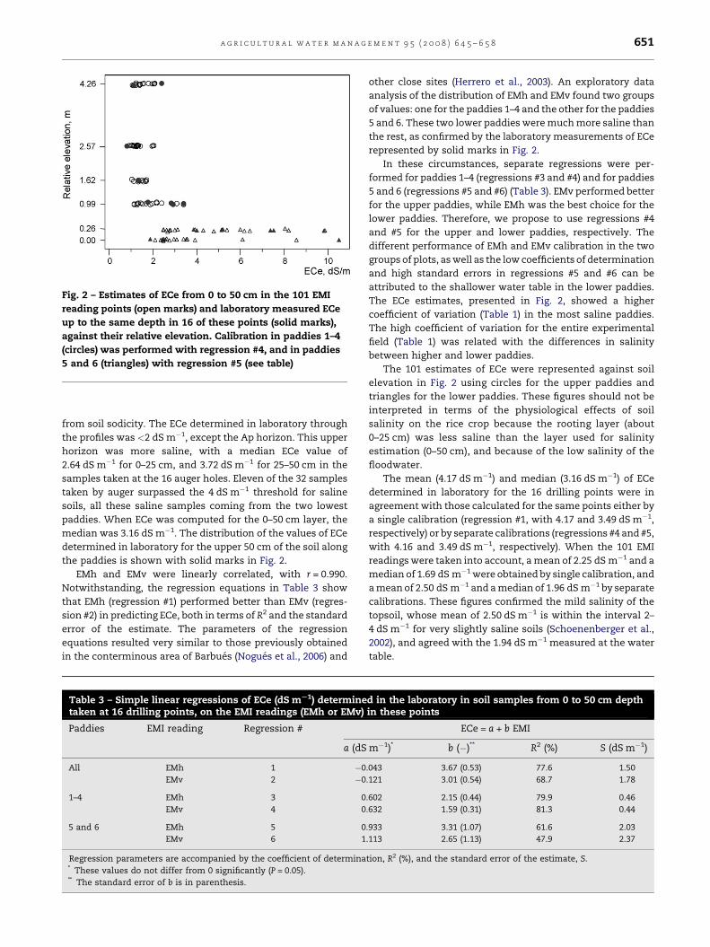
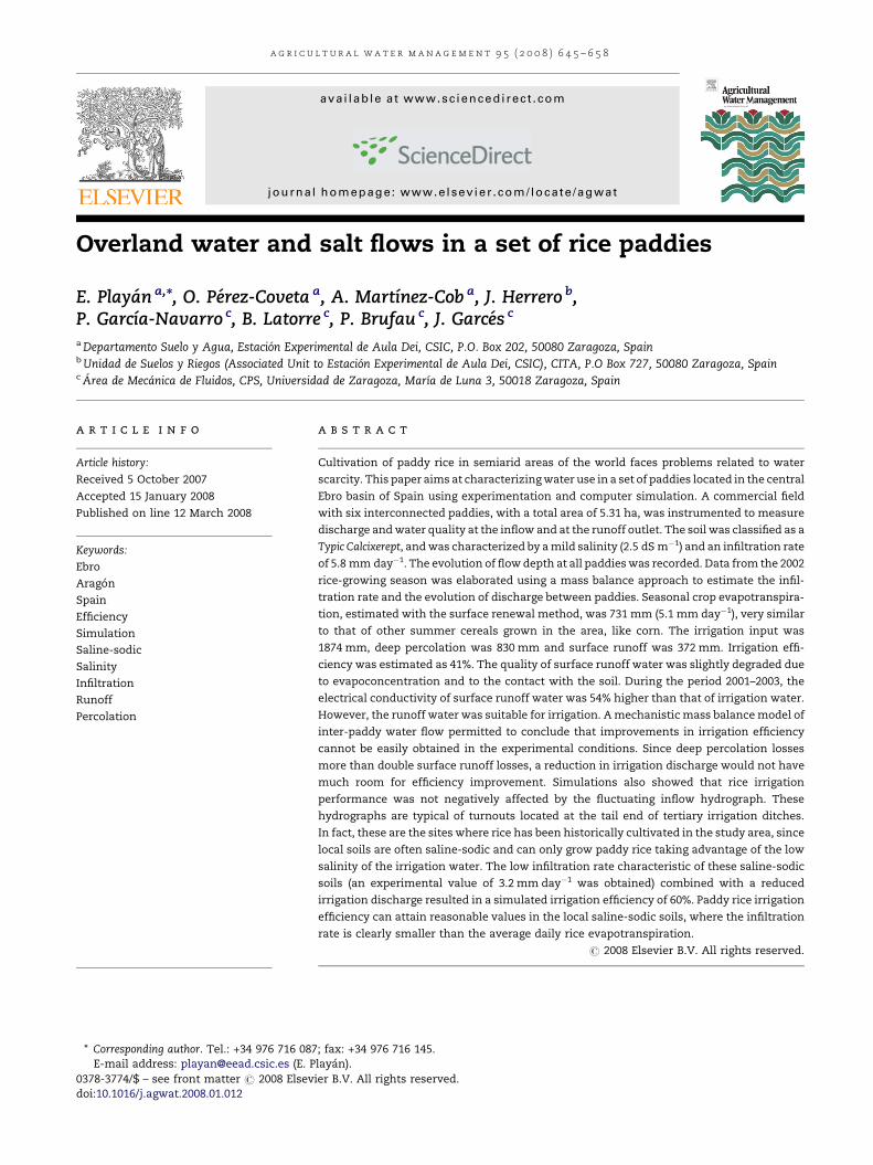
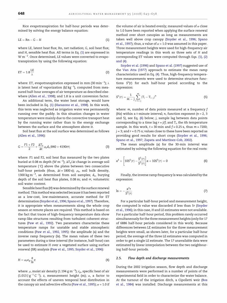
Fig. 2 – Estimates of ECe from 0 to 50 cm in the 101 EMI

reading points (open marks) and laboratory measured ECe

up to the same depth in 16 of these points (solid marks),

against their relative elevation. Calibration in paddies 1–4

(circles) was performed with regression #4, and in paddies

5 and 6 (triangles) with regression #5 (see table)


from soil sodicity. The ECe determined in laboratory through

the profiles was <2 dS m�1, except the Ap horizon. This upper

horizon was more saline, with a median ECe value of

2.64 dS m�1 for 0–25 cm, and 3.72 dS m�1 for 25–50 cm in the

samples taken at the 16 auger holes. Eleven of the 32 samples

taken by auger surpassed the 4 dS m�1 threshold for saline

soils, all these saline samples coming from the two lowest

paddies. When ECe was computed for the 0–50 cm layer, the

median was 3.16 dS m�1. The distribution of the values of ECe

determined in laboratory for the upper 50 cm of the soil along

the paddies is shown with solid marks in Fig. 2.

EMh and EMv were linearly correlated, with r = 0.990.

Notwithstanding, the regression equations in Table 3 show

that EMh (regression #1) performed better than EMv (regres-

sion #2) in predicting ECe, both in terms of R2 and the standard

error of the estimate. The parameters of the regression

equations resulted very similar to those previously obtained

in the conterminous area of Barbues (Nogues et al., 2006) and

Table 3 – Simple linear regressions of ECe (dS mS1) determinetaken at 16 drilling points, on the EMI readings (EMh or EMv)

Paddies EMI reading Regression #

a (dS

All EMh 1 �0

EMv 2 �0

1–4 EMh 3 0

EMv 4 0

5 and 6 EMh 5 0

EMv 6 1

Regression parameters are accompanied by the coefficient of determina* These values do not differ from 0 significantly (P = 0.05).** The standard error of b is in parenthesis.

other close sites (Herrero et al., 2003). An exploratory data

analysis of the distribution of EMh and EMv found two groups

of values: one for the paddies 1–4 and the other for the paddies

5 and 6. These two lower paddies were much more saline than

the rest, as confirmed by the laboratory measurements of ECe

represented by solid marks in Fig. 2.

In these circumstances, separate regressions were per-

formed for paddies 1–4 (regressions #3 and #4) and for paddies

5 and 6 (regressions #5 and #6) (Table 3). EMv performed better

for the upper paddies, while EMh was the best choice for the

lower paddies. Therefore, we propose to use regressions #4

and #5 for the upper and lower paddies, respectively. The

different performance of EMh and EMv calibration in the two

groups of plots, as well as the low coefficients of determination

and high standard errors in regressions #5 and #6 can be

attributed to the shallower water table in the lower paddies.

The ECe estimates, presented in Fig. 2, showed a higher

coefficient of variation (Table 1) in the most saline paddies.

The high coefficient of variation for the entire experimental

field (Table 1) was related with the differences in salinity

between higher and lower paddies.

The 101 estimates of ECe were represented against soil

elevation in Fig. 2 using circles for the upper paddies and

triangles for the lower paddies. These figures should not be

interpreted in terms of the physiological effects of soil

salinity on the rice crop because the rooting layer (about

0–25 cm) was less saline than the layer used for salinity

estimation (0–50 cm), and because of the low salinity of the

floodwater.

The mean (4.17 dS m�1) and median (3.16 dS m�1) of ECe

determined in laboratory for the 16 drilling points were in

agreement with those calculated for the same points either by

a single calibration (regression #1, with 4.17 and 3.49 dS m�1,

respectively) or by separate calibrations (regressions #4 and #5,

with 4.16 and 3.49 dS m�1, respectively). When the 101 EMI

readings were taken into account, a mean of 2.25 dS m�1 and a

median of 1.69 dS m�1 were obtained by single calibration, and

a mean of 2.50 dS m�1 and a median of 1.96 dS m�1 by separate

calibrations. These figures confirmed the mild salinity of the

topsoil, whose mean of 2.50 dS m�1 is within the interval 2–

4 dS m�1 for very slightly saline soils (Schoenenberger et al.,

2002), and agreed with the 1.94 dS m�1 measured at the water

table.

d in the laboratory in soil samples from 0 to 50 cm depthin these points

ECe = a + b EMI

m�1)* b (�)** R2 (%) S (dS m�1)

.043 3.67 (0.53) 77.6 1.50

.121 3.01 (0.54) 68.7 1.78

.602 2.15 (0.44) 79.9 0.46

.632 1.59 (0.31) 81.3 0.44

.933 3.31 (1.07) 61.6 2.03

.113 2.65 (1.13) 47.9 2.37

tion, R2 (%), and the standard error of the estimate, S.


3.2. Irrigation and runoff water quality

The chemical characterisation of irrigation and runoff water is

presented in Table 4. Results were quite similar during the 3

years of study. This seems to be due to the stable, low mineral

load of the irrigation water, which is transported from the

Pyrenees through a network of mountain rivers and lowland

Table 4 – Chemical characterization of the irrigation and runoff2003, and for the average of the 3 years

2001

Irrigationa Runoffa

Electrical conductivity (EC, dS m�1) n 8 14

Mean 0.26 0.33

CV 13 16

pH n 0 0

Mean – –

CV – –

Major anions (mmol c L�1)b

Cl� n 8 14

Mean 0.26 0.61

CV 40 39

SO42� n 8 14

Mean 0.57 0.61

CV 11 40

HCO3� n 8 14

Mean ip ip

CV – –

Major cations (mmol c L�1)

Ca2+ n 8 14

Mean 1.16 1.09

CV 7 31

Mg2+ n 8 14

Mean 0.58 0.78

CV 14 15

Na+ n 8 14

Mean 0.30 0.72

CV 40 39

K+ n 8 14

Mean 0.06 0.06

CV 37 47

Na+/Ca2+ ratio 0.26 0.66

SAR from the above

means of Na+, Ca2+ and Mg2+

0.3 0.7

Nutrients (mg L�1)

NO3� n 5 3

Mean 0.3 3.6

CV 46 131

NH4+ n 0 2

Mean – 3.1

CV – 6

Number of samples (n), mean and coefficient of variation (CV, %) are prov

and nutrients. (ip) Inappreciable. The table also includes the Na+/Ca2+ raa Kind of water.b CO3

2� was inappreciable (concentration below the detection threshold

canals. The years of continuous rice cultivation add stability to

the chemical properties of the runoff water. Due to this time

stability, average results from the 3 years of study will be

discussed, with some references to particular years.

The irrigation water electrical conductivity averaged

0.24 dS m�1, with an interannual coefficient of variation of

22%. Runoff water averaged 0.37 dS m�1. This increment in

water in the set of rice paddies for the years 2001, 2002 and

2002 2003 2001–2003

Irrigation Runoff Irrigation Runoff Irrigation Runoff

11 12 18 17 37 43

0.27 0.5 0.18 0.29 0.24 0.37

9 26 43 50 22 31

11 12 0 0 11 12

8.2 7.5 – – 8.2 7.5

2 2 – – 2 2

20 20 18 17 46 51

0.12 0.67 0.24 0.78 0.21 0.69

71 114 73 76 61 76

20 20 18 17 46 51

0.31 0.41 0.46 0.56 0.45 0.53

63 123 42 79 39 81

20 20 18 17 18 17

ip ip 1.27 1.63 1.27 1.63

– – 58 78 58 78

16 17 18 17 42 48

0.75 0.99 0.83 1.03 0.91 1.04

64 74 77 96 49 67

14 18 18 17 40 49

0.39 0.61 0.67 0.78 0.55 0.72

36 65 42 41 31 40

16 19 18 17 42 50

0.18 0.96 0.35 0.97 0.28 0.88

34 88 65 59 46 62

20 20 18 17 46 51

0.03 0.03 0.06 0.13 0.05 0.07

55 72 70 81 54 67

0.24 0.97 0.43 0.93 0.30 0.85

0.2 1.1 0.4 1.0 0.3 0.9

5 1 5 0 15 4

0.1 1.1 3.4 – 1.27 2.35

51 0 55 – 51 66

15 6 7 6 22 14

0.2 0.5 0.4 0.9 0.3 1.5

45 79 35 95 40 60

ided for electrical conductivity, pH and for the concentration of ions

tio and the Sodium Adsorption Ratio (SAR).

of the laboratory equipment) in all samples.

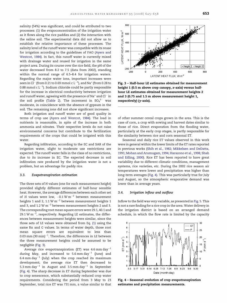
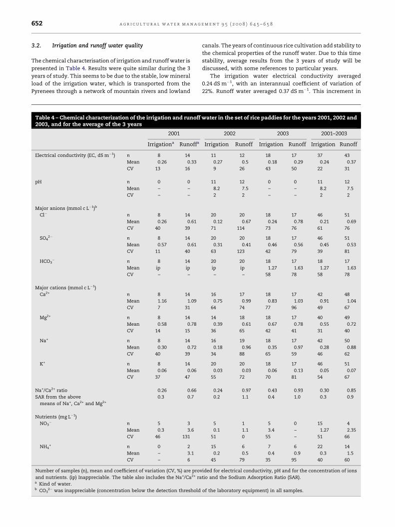
Fig. 3 – Half-hour LE estimates obtained for measurement

height 1 (0.5 m above crop canopy, x-axis) versus half-

hour LE estimates obtained for measurement heights 2

and 3 (0.75 and 1.5 m above measurement height 1,

respectively) (y-axis).

Fig. 4 – Seasonal evolution of crop evapotranspiration

estimates and precipitation measurements.


salinity (54%) was significant, and could be attributed to two

processes: (1) the evapoconcentration of the irrigation water

as it flows along the rice paddies and (2) the interaction with

the saline soil. The experimental data did not allow us to

establish the relative importance of these processes. The

salinity level of the runoff water was compatible with its reuse

for irrigation according to the guidelines of FAO (Ayers and

Westcot, 1984). In fact, this runoff water is currently mixed

with drainage water and reused for irrigation in the same

project area. During its course over the rice field, the pH of the

water decreased from 8.2 to 7.5 (data from 2002), standing

within the normal range of 6.5–8.4 for irrigation waters.

Regarding the major water ions, important increases were

seen in Cl� (from 0.21 to 0.69 mmol c L�1), and Na+ (from 0.28 to

0.88 mmol c L�1). Sodium chloride could be partly responsible

for the increase in electrical conductivity between irrigation

and runoff water, agreeing with the presence of Na+ and Cl� in

the soil profile (Table 2). The increment in SO42� was

moderate, in coincidence with the absence of gypsum in the

soil. The remaining ions did not show significant increases.

Both irrigation and runoff water are of good quality in

terms of crop use (Ayers and Westcot, 1984). The load in

nutrients is reasonable, in spite of the increase in both

ammonia and nitrates. Their respective levels do not raise

environmental concerns but contribute to the fertilization

requirements of the crops that could be irrigated with this

water.

Regarding infiltration, according to the EC and SAR of the

irrigation water, slight to moderate use restrictions are

expected. The runoff water falls in the class of no restrictions,

due to its increase in EC. The expected decrease in soil

infiltration rate produced by the irrigation water is not a

problem, but an advantage for paddy rice.

3.3. Evapotranspiration estimation

The three sets of H values (one for each measurement height)

provided slightly different estimates of half-hour sensible

heat. However, the average differences between each other set

of H values were low, �0.1 W m�2 between measurement

heights 1 and 2, 1.1 W m�2 between measurement heights 1

and 3, and 1.2 W m�2 between measurement heights 2 and 3.

The corresponding root mean square errors were 29.1, 40.1 and

29.1 W m�2, respectively. Regarding LE estimates, the differ-

ences between measurement heights were similar, since the

three sets of LE values were obtained from Eq. (1) using the

same Rn and G values. In terms of water depth, those root

mean square errors are equivalent to less than

0.03 mm (30 min)�1. Therefore, the differences in LE between

the three measurement heights could be assumed to be

negligible (Fig. 3).

Average rice evapotranspiration (ET) was 4.6 mm day�1

during May, and increased to 5.6 mm day�1 (June) and

6.4 mm day�1 (July) when the crop reached its maximum

development; the average rice ET then decreased to

5.3 mm day�1 in August and 3.5 mm day�1 in September

(Fig. 4). The sharp decrease in ET during September was due

to crop senescence, which substantially reduced crop water

requirements. Considering the period from 3 May to 23

September, total rice ET was 731 mm, a value similar to that

of other summer cereal crops grown in the area. This is the

case of corn, a crop with sowing and harvest dates similar to

those of rice. Direct evaporation from the flooding water,

particularly at the early crop stages, is partly responsible for

the similarity between rice and corn seasonal ET.

Seasonal and daily rice ET values observed in this work

were in general within the lower limits of the ET rates reported

in previous works (Shih et al., 1982; Mikkelsen and DeDatta,

1991; Mohan and Arumugam, 1994; Harazono et al., 1998; Shah

and Edling, 2000). Rice ET has been reported to have great

variability due to different climatic conditions, management

systems, rice varieties, etc. During the 2002 rice season air

temperatures were lower and precipitation was higher than

long-term averages (Fig. 4). This was particularly true for July

and August, so the atmospheric evaporative demand was

lower than in average years.

3.4. Irrigation inflow and outflow

Inflow to the field was very variable, as presented in Fig. 5. This

is not a rare finding for a rice crop in the area. Water delivery in

the irrigation district is based on an arranged demand

schedule, in which the flow rate is limited by the capacity

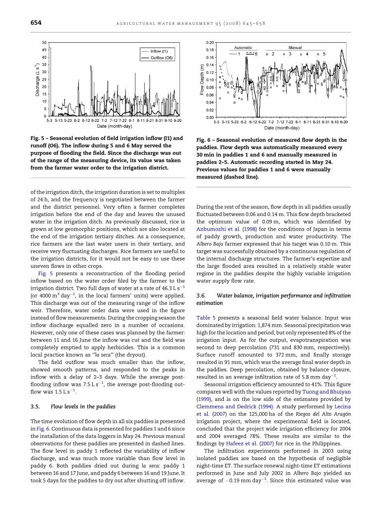
Fig. 5 – Seasonal evolution of field irrigation inflow (I1) and

runoff (O6). The inflow during 5 and 6 May served the

purpose of flooding the field. Since the discharge was out

of the range of the measuring device, its value was taken

from the farmer water order to the irrigation district.

Fig. 6 – Seasonal evolution of measured flow depth in the

paddies. Flow depth was automatically measured every

30 min in paddies 1 and 6 and manually measured in

paddies 2–5. Automatic recording started in May 24.

Previous values for paddies 1 and 6 were manually

measured (dashed line).


of the irrigation ditch, the irrigation duration is set to multiples

of 24 h, and the frequency is negotiated between the farmer

and the district personnel. Very often a farmer completes

irrigation before the end of the day and leaves the unused

water in the irrigation ditch. As previously discussed, rice is

grown at low geomorphic positions, which are also located at

the end of the irrigation tertiary ditches. As a consequence,

rice farmers are the last water users in their tertiary, and

receive very fluctuating discharges. Rice farmers are useful to

the irrigation districts, for it would not be easy to use these

uneven flows in other crops.

Fig. 5 presents a reconstruction of the flooding period

inflow based on the water order filed by the farmer to the

irrigation district. Two full days of water at a rate of 46.3 L s�1

(or 4000 m3 day�1, in the local farmers’ units) were applied.

This discharge was out of the measuring range of the inflow

weir. Therefore, water order data were used in the figure

instead of flow measurements. During the cropping season the

inflow discharge equalled zero in a number of occasions.

However, only one of these cases was planned by the farmer:

between 11 and 16 June the inflow was cut and the field was

completely emptied to apply herbicides. This is a common

local practice known as ‘‘la seca’’ (the dryout).

The field outflow was much smaller than the inflow,

showed smooth patterns, and responded to the peaks in

inflow with a delay of 2–3 days. While the average post-

flooding inflow was 7.5 L s�1, the average post-flooding out-

flow was 1.5 L s�1.

3.5. Flow levels in the paddies

The time evolution of flow depth in all six paddies is presented

in Fig. 6. Continuous data is presented for paddies 1 and 6 since

the installation of the data loggers in May 24. Previous manual

observations for these paddies are presented in dashed lines.

The flow level in paddy 1 reflected the variability of inflow

discharge, and was much more variable than flow level in

paddy 6. Both paddies dried out during la seca: paddy 1

between 16 and 17 June, and paddy 6 between 16 and 19 June. It

took 5 days for the paddies to dry out after shutting off inflow.

During the rest of the season, flow depth in all paddies usually

fluctuated between 0.06 and 0.14 m. This flow depth bracketed

the optimum value of 0.09 m, which was identified by

Anbumozhi et al. (1998) for the conditions of Japan in terms

of paddy growth, production and water productivity. The

Albero Bajo farmer expressed that his target was 0.10 m. This

target was successfully obtained by a continuous regulation of

the internal discharge structures. The farmer’s expertise and

the large flooded area resulted in a relatively stable water

regime in the paddies despite the highly variable irrigation

water supply flow rate.

3.6. Water balance, irrigation performance and infiltrationestimation

Table 5 presents a seasonal field water balance. Input was

dominated by irrigation: 1,874 mm. Seasonal precipitation was

high for the location and period, but only represented 8% of the

irrigation input. As for the output, evapotranspiration was

second to deep percolation (731 and 830 mm, respectively).

Surface runoff amounted to 372 mm, and finally storage

resulted in 91 mm, which was the average final water depth in

the paddies. Deep percolation, obtained by balance closure,

resulted in an average infiltration rate of 5.8 mm day�1.

Seasonal irrigation efficiency amounted to 41%. This figure

compares well with the values reported by Tuong and Bhuiyan

(1999), and is on the low side of the estimates provided by

Clemmens and Dedrick (1994). A study performed by Lecina

et al. (2007) on the 125,000 ha of the Riegos del Alto Aragon

irrigation project, where the experimental field is located,

concluded that the project wide irrigation efficiency for 2004

and 2004 averaged 78%. These results are similar to the

findings by Hafeez et al. (2007) for rice in the Philippines.

The infiltration experiments performed in 2003 using

isolated paddies are based on the hypothesis of negligible

night-time ET. The surface renewal night-time ET estimations

performed in June and July 2002 in Albero Bajo yielded an

average of �0.19 mm day�1. Since this estimated value was

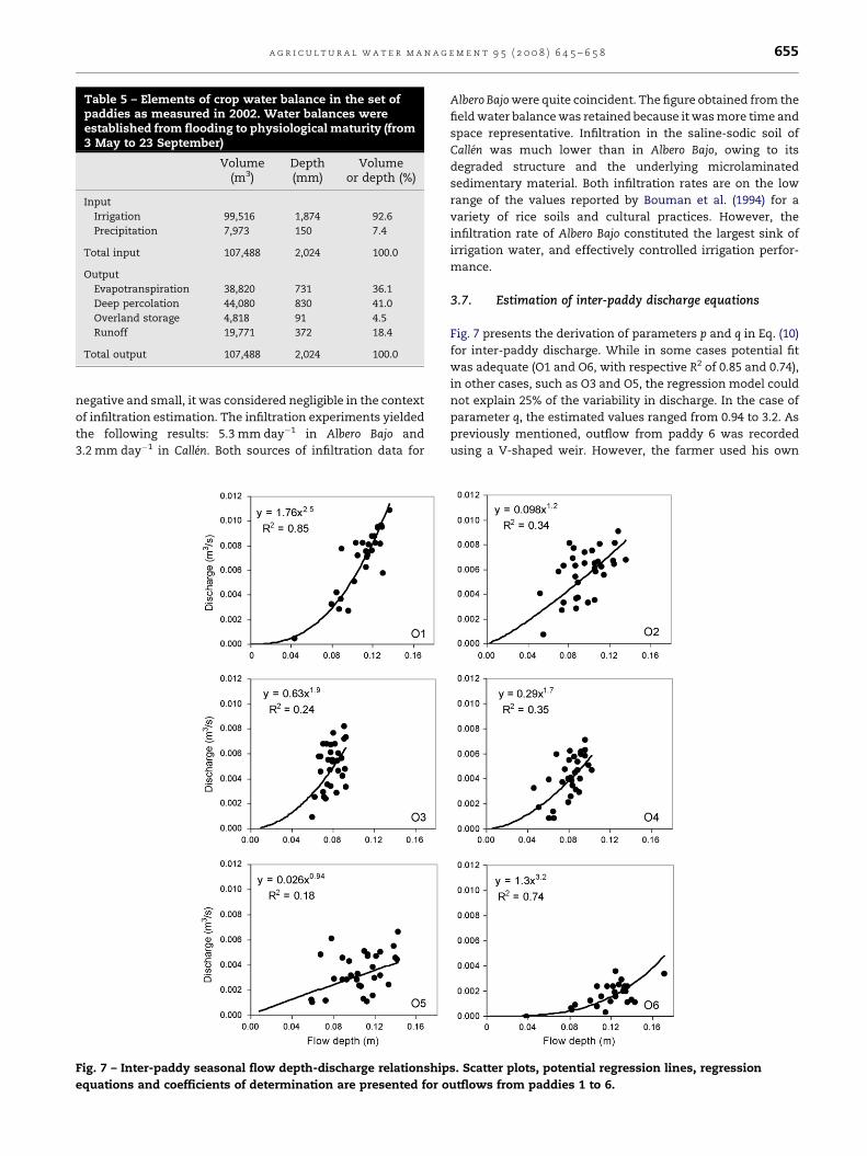
Table 5 – Elements of crop water balance in the set ofpaddies as measured in 2002. Water balances wereestablished from flooding to physiological maturity (from3 May to 23 September)

Volume(m3)

Depth(mm)

Volumeor depth (%)

Input

Irrigation 99,516 1,874 92.6

Precipitation 7,973 150 7.4

Total input 107,488 2,024 100.0

Output

Evapotranspiration 38,820 731 36.1

Deep percolation 44,080 830 41.0

Overland storage 4,818 91 4.5

Runoff 19,771 372 18.4

Total output 107,488 2,024 100.0


negative and small, it was considered negligible in the context

of infiltration estimation. The infiltration experiments yielded

the following results: 5.3 mm day�1 in Albero Bajo and

3.2 mm day�1 in Callen. Both sources of infiltration data for

Fig. 7 – Inter-paddy seasonal flow depth-discharge relationship

equations and coefficients of determination are presented for o

Albero Bajo were quite coincident. The figure obtained from the

field water balance was retained because it was more time and

space representative. Infiltration in the saline-sodic soil of

Callen was much lower than in Albero Bajo, owing to its

degraded structure and the underlying microlaminated

sedimentary material. Both infiltration rates are on the low

range of the values reported by Bouman et al. (1994) for a

variety of rice soils and cultural practices. However, the

infiltration rate of Albero Bajo constituted the largest sink of

irrigation water, and effectively controlled irrigation perfor-

mance.

3.7. Estimation of inter-paddy discharge equations

Fig. 7 presents the derivation of parameters p and q in Eq. (10)

for inter-paddy discharge. While in some cases potential fit

was adequate (O1 and O6, with respective R2 of 0.85 and 0.74),

in other cases, such as O3 and O5, the regression model could

not explain 25% of the variability in discharge. In the case of

parameter q, the estimated values ranged from 0.94 to 3.2. As

previously mentioned, outflow from paddy 6 was recorded

using a V-shaped weir. However, the farmer used his own

s. Scatter plots, potential regression lines, regression

utflows from paddies 1 to 6.

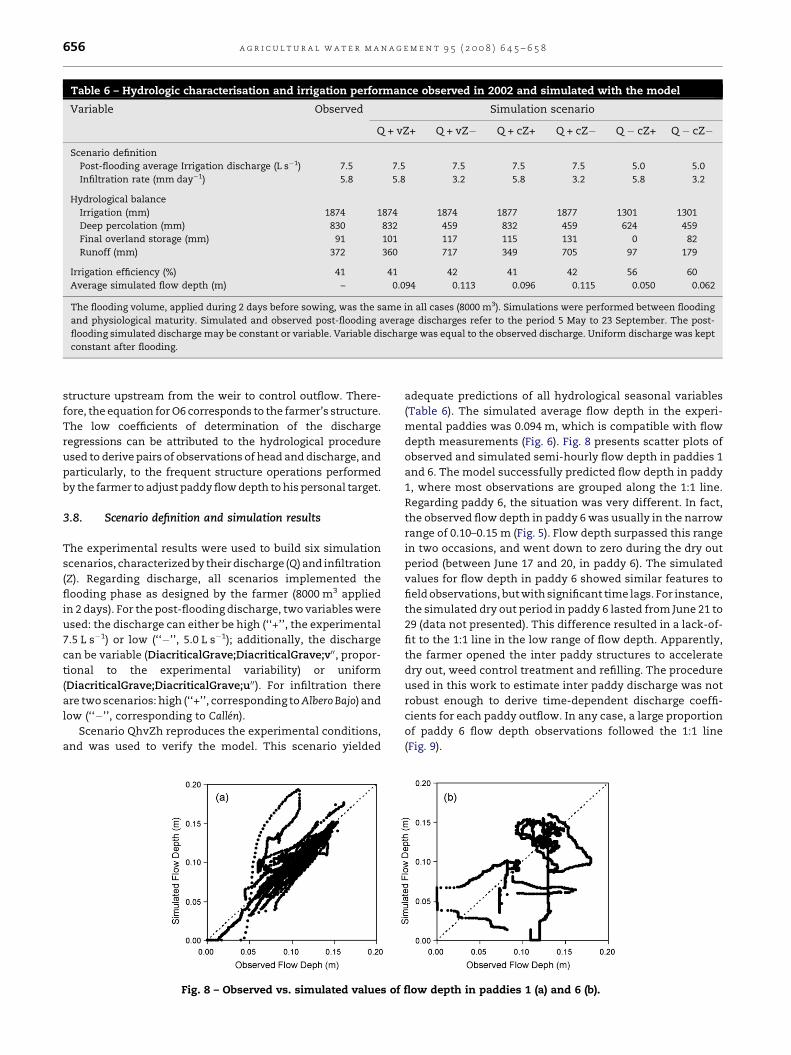
Table 6 – Hydrologic characterisation and irrigation performance observed in 2002 and simulated with the model

Variable Observed Simulation scenario

Q + vZ+ Q + vZ� Q + cZ+ Q + cZ� Q � cZ+ Q � cZ�

Scenario definition

Post-flooding average Irrigation discharge (L s�1) 7.5 7.5 7.5 7.5 7.5 5.0 5.0

Infiltration rate (mm day�1) 5.8 5.8 3.2 5.8 3.2 5.8 3.2

Hydrological balance

Irrigation (mm) 1874 1874 1874 1877 1877 1301 1301

Deep percolation (mm) 830 832 459 832 459 624 459

Final overland storage (mm) 91 101 117 115 131 0 82

Runoff (mm) 372 360 717 349 705 97 179

Irrigation efficiency (%) 41 41 42 41 42 56 60

Average simulated flow depth (m) – 0.094 0.113 0.096 0.115 0.050 0.062

The flooding volume, applied during 2 days before sowing, was the same in all cases (8000 m3). Simulations were performed between flooding

and physiological maturity. Simulated and observed post-flooding average discharges refer to the period 5 May to 23 September. The post-

flooding simulated discharge may be constant or variable. Variable discharge was equal to the observed discharge. Uniform discharge was kept

constant after flooding.


structure upstream from the weir to control outflow. There-

fore, the equation for O6 corresponds to the farmer’s structure.

The low coefficients of determination of the discharge

regressions can be attributed to the hydrological procedure

used to derive pairs of observations of head and discharge, and

particularly, to the frequent structure operations performed

by the farmer to adjust paddy flow depth to his personal target.

3.8. Scenario definition and simulation results

The experimental results were used to build six simulation

scenarios, characterized by their discharge (Q) and infiltration

(Z). Regarding discharge, all scenarios implemented the

flooding phase as designed by the farmer (8000 m3 applied

in 2 days). For the post-flooding discharge, two variables were

used: the discharge can either be high (‘‘+’’, the experimental

7.5 L s�1) or low (‘‘�’’, 5.0 L s�1); additionally, the discharge

can be variable (DiacriticalGrave;DiacriticalGrave;v00, propor-

tional to the experimental variability) or uniform

(DiacriticalGrave;DiacriticalGrave;u00). For infiltration there

are two scenarios: high (‘‘+’’, corresponding toAlbero Bajo) and

low (‘‘�’’, corresponding to Callen).

Scenario QhvZh reproduces the experimental conditions,

and was used to verify the model. This scenario yielded

Fig. 8 – Observed vs. simulated values of

adequate predictions of all hydrological seasonal variables

(Table 6). The simulated average flow depth in the experi-

mental paddies was 0.094 m, which is compatible with flow

depth measurements (Fig. 6). Fig. 8 presents scatter plots of

observed and simulated semi-hourly flow depth in paddies 1

and 6. The model successfully predicted flow depth in paddy

1, where most observations are grouped along the 1:1 line.

Regarding paddy 6, the situation was very different. In fact,

the observed flow depth in paddy 6 was usually in the narrow

range of 0.10–0.15 m (Fig. 5). Flow depth surpassed this range

in two occasions, and went down to zero during the dry out

period (between June 17 and 20, in paddy 6). The simulated

values for flow depth in paddy 6 showed similar features to

field observations, but with significant time lags. For instance,

the simulated dry out period in paddy 6 lasted from June 21 to

29 (data not presented). This difference resulted in a lack-of-

fit to the 1:1 line in the low range of flow depth. Apparently,

the farmer opened the inter paddy structures to accelerate

dry out, weed control treatment and refilling. The procedure

used in this work to estimate inter paddy discharge was not

robust enough to derive time-dependent discharge coeffi-

cients for each paddy outflow. In any case, a large proportion

of paddy 6 flow depth observations followed the 1:1 line

(Fig. 9).

flow depth in paddies 1 (a) and 6 (b).

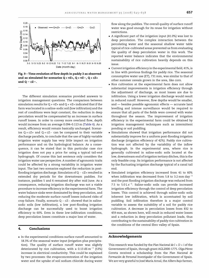
Fig. 9 – Time evolution of flow depth in paddy 3 as observed

and as simulated for scenarios Q + vZ+, Q + vZS, Q + cZ+

and Q S cZS.


The different simulation scenarios provided answers to

irrigation management questions. The comparison between

simulation results for Q + vZ+ and Q + vZ+ indicated that if the

farm was located in a saline-sodic soil (low infiltration) and the

rest of conditions were kept constant, the reduction in deep

percolation would be compensated by an increase in surface

runoff losses. In order to convey more overland flow, depth

would increase from an average 0.094–0.113 m (Table 6). As a

result, efficiency would remain basically unchanged. Scenar-

ios Q + cZ+ and Q + cZ� can be compared to their variable

discharge parallels, to conclude that the use of highly variable

irrigation water supply has very little impact on irrigation

performance and on the hydrological balance. As a conse-

quence, it can be stated that in this particular case rice

irrigation does not pay a price for using a typical tail-end

hydrograph. Of course this last sentence only considers the

irrigation water use perspective. A number of agronomic traits

could be affected by a strong variability in irrigation water

input. The last two scenarios explored the reduction in post-

flooding irrigation discharge. Simulation of Q � cZ+ resulted in

extended dry periods for the downstream paddies. For

instance, paddies 5 and 6 remained dry after mid June. As a

consequence, reducing irrigation discharge was not a viable

procedure to increase efficiency in the experimental farm. The

water balance sinks were dominated by deep percolation, and

reducing the moderate surface runoff losses induced risks of

crop failure. Finally, scenario Q � cZ� showed that in saline-

sodic soils (low infiltration), a low post-flooding irrigation

discharge can be successfully used to boost irrigation

efficiency to 60%. Even in these low-infiltration conditions,

deep percolation losses constitute a major loss of water.

4. Conclusions

� In the experimental conditions surface runoff amounted to

18.3% of the seasonal water input (irrigation plus precipita-

tion). The quality of surface runoff water was slightly

deteriorated by rice cultivation, with a 0.13 dS m�1 (53%)

increase in electrical conductivity. This could be explained

by two processes: the evapoconcentration of the irrigation

water and the uptake of soil sodium chloride during water

flow along the paddies. The overall quality of surface runoff

water was good enough for its reuse for irrigation without

restrictions.

� A
significant part of the irrigation input (41.0%) was lost to
deep percolation. The complex interaction between the

percolating water and the seasonal shallow water table

typical of rice-cultivated areas prevented us from evaluating

the quality of deep percolation water in this work. The

reported water balance indicates that the environmental

sustainability of rice cultivation heavily depends on this

issue.

� C
urrent irrigation efficiency in the experimental field, 41%, is
in line with previous findings for paddy rice. The seasonal

consumptive water use (ET), 731 mm, was similar to that of

other summer cereals grown in the area, like corn.

� R
ice cultivation at the experimental farm does not allow
substantial improvements in irrigation efficiency through

the adjustment of discharge, as most losses are due to

infiltration. Using a lower irrigation discharge would result

in reduced runoff. However, flow depths would be smaller,

and — besides possible agronomic effects — accurate land

levelling and intense surveillance would be required to

ensure that all parts of the fields were covered with water

throughout the season. The improvement of irrigation

efficiency in the experimental farm could be obtained by

irrigation management techniques such as intermittent

ponding or soil puddling.

� S
imulations showed that irrigation performance did not
substantially improve for a uniform post-flooding irrigation

discharge (irrigation efficiency of 42%). Paddy rice cultiva-

tion was not affected by the variability of the inflow

hydrograph. In the experimental area, where rice is

generally cultivated in saline-sodic soils located at the

low, downstream end of irrigation tertiary ditches, this is the

only feasible crop. Its irrigation performance is not affected

by the fluctuating irrigation discharge typical of a canal tail

end.

� S
imulated irrigation efficiency increased from 41 to 60%
when infiltration was decreased from 5.8 to 3.2 mm day�1

and the post flooding irrigation discharge was reduced from

7.5 to 5.0 L s�1. Saline-sodic soils can provide increased

irrigation efficiency through the control of deep percolation

losses. This control is achieved through saline-sodic soils

inherent low infiltration, which is accentuated by soil

puddling. Soil infiltration therefore is a major control

variable to assess the suitability of a soil for paddy rice

cultivation. A decrease in percolation losses from 832 to

459 mm, as shown here, will result in reduced water losses

and a reduction in deep percolation pollutant loads, thus

contributing to the sustainability of paddy rice cultivation in

the conditions of the central Ebro valley of Spain.

Acknowledgements

This research was funded by the Plan Nacional de I + D + i of the

Government of Spain, through grant AGL2000-1775. Olga Perez

Coveta received a scholarship from the Plan Nacional de

Formacion de Personal Investigador of the Government of Spain.

We are very grateful to Jose Marıa Arnal, theAlbero Bajo farmer,


for his cooperation throughout the experiments. Finally, it

would have been impossible to complete this work without the

enthusiastic support from our field team: Miguel Izquierdo,

Jesus Gaudo and Daniel Mayoral.

r e f e r e n c e s

Allen, R.G., Pruitt, W.O., Businger, J.A., 1996. Evapotranspirationand transpiration. In: Heggen, R.J., Wootton, T.P., Cecilio,C.B., Fowler, L.C., Hui, S.L. (Eds.), Hydrology Handbook. 2nded. American Society of Civil Engineers, New York, NY, USA,pp. 125–252.

Allen, R.G., Pereira, L.S., Raes D., Smith M. 1998. Cropevapotranspiration: guidelines for computing crop waterrequeriments. FAO Irrigation and Drainage Paper 56. FAO,Rome, Italy.

Anbumozhi, V., Yamaji, E., Tabichhi, T., 1998. Rice crop growthand yield as influenced by changes in ponding water depth,water regime and fertigation level. Agric. Water Manage. 37(3), 241–253.

Ayers, R.S., Westcot, D.W., 1984. Water quality for agriculture.FAO Irrigation and Drainage Paper, 29 Rev. 1. Reprinted1989, 1994. FAO, Rome.

Beecher, H.G., Hume, I.H., Dunn, B.W., 2002. Improved methodfor assessing rice soil suitability to restrict recharge. Aust. J.Exp. Agric. 42 (3), 297–307.

Belder, P., Bouman, B.A.M., Cabangon, R., Guıan, L., Quilang,E.J.P., Yuanhua, L., Spiertz, J.H.J., Tuong, T.P., 2004. Effect ofwater-saving irrigation on rice yield and water use in typicallowland conditions in Asia. Agric. Water Manage. 65 (3),193–210.

Bos, M.G., Replogle, J.A., Clemmens, A.J., 1984. Flow MeasuringFlumes for Open Channel Systems. John Wiley & sons Inc.,New York, USA.

Bouman, B.A.M., Wopereis, M.C.S., Kropff, M.J., ten Berge,H.F.M., Tuong, T.P., 1994. Agric. Water Manage. 26 (4) 291–304.

Burt, C.M., Clemmens, A.J., Strelkoff, T.S., Solomon, K.H.,Bliesner, R.D., Hardy, L.A., Howell, T.A., Eisenhauer, D.E.,1997. Irrigation performance measures: efficiency anduniformity. J. Irrig. Drain. Div., ASCE 123 (6), 423–442.

Clemmens, A.J., Dedrick, A.R., 1994. Irrigation techniques andevaluations. In: Tanji, K.K., Yaron, B. (Eds.), Adv. Series inAgricultural Sciences, vol. 22. Springer-Verlag, Berlin, pp.64–103.

Faci, J.M., Martınez-Cob, A., 1991. Calculo de laevapotranspiracion de referencia en Aragon. Departamentode Agricultura. Gobierno de Aragon, Zaragoza, Spain.

Hafeez, M.M., Bouman, B.A.M., Van de Giesen, N., Vlek, P., 2007.Scale effects on water use and water productivity in arice-based irrigation system (UPRIIS) in the Philippines.Agric. Water Manage. 92 (1/2), 81–89.

Harazono, Y., Kim, J., Miyata, A., Choi, T., Yun, J.I., Kim, J.W.,1998. Measurement of energy budget components duringthe International Rice Experiment (IREX) in Japan. Hydrol.Processes 12, 2081–2092.

Herrero, J., Ba, A.A., Aragues, R., 2003. Soil salinity and itsdistribution determined by soil sampling andelectromagnetic techniques. Soil Use Manage. 19 (2), 119–126.

Jarauta, E., 1989. Modelos matematicos de regimen de humedaddel suelo. PhD Thesis. Universidad Politecnica de Barcelona,Spain.

Keller, A., Keller, J., Seckler, D., 1996. Integrated water resourcesystems: theory and policy implications. Research Report 3.

International Irrigation Management Institute (IIMI),Colombo, Sri Lanka.

Kukal, S.S., Aggarwal, G.C., 2002. Percolation losses of water inrelation to puddling intensity and depth in a sandy loamrice (Oryza sativa) field. Agric. Water Manage. 57 (1), 49–59.

Lecina, S., Zapata, N., Playan, E., Salvador, R., Faci, J.M., Mantero,I., Cavero, J., Andres, J., 2007. Consecuencias de lamodernizacion del regadıo sobre el aprovechamiento delagua en Riegos del Alto Aragon. In: XXV Congreso Nacionalde Riegos. Comite Espanol de Riegos y Drenajes, Pamplona,Spain.

McCauley, G.N., 1990. Sprinkler vs. flood irrigation in traditionalrice production regions of Southeast Texas. Agron. J. 82 (4),677–682.

Mikkelsen, D.S., DeDatta, S.K., 1991. Rice culture. In: Luh, B.S.(Ed.), Rice Production, vol. 1. Van Nostrand Reinhold, NewYork, NY, USA, pp. 103–186.

Mohan, S., Arumugam, N., 1994. Irrigation crop coefficients forlowland rice. Irrig. Drain. Sys. 8, 159–176.

Nogues, J., Herrero, J., 2003. The impact of transition from floodto sprinkling irrigation on water district consumption. J.Hydrol. 276, 37–52.

Nogues, J., Robinson, D.A., Herrero, J., 2006. Incorporatingelectromagnetic induction methods into regional soilsalinity survey of irrigation districts. Soil Sci. Soc. Am. J. 70,2075–2085.

Paw, U.K.T., Brunet, Y., Collineau, S., Shaw, R.H., Maitani, T.,Qiu, J., Hipps, L., 1992. On coherent structures in turbulenceabove and within agricultural plant canopies. Agric. For.Meteorol. 61, 55–68.

Paw, U.K.T., Qiu, J., Su, H.B., Watanabe, T., Brunet, Y., 1995.Surface renewal analysis: a new method to obtain scalarfluxes without velocity data. Agric. For. Meteorol. 74,119–137.

Perry, C.J., 1999. The IWMI water resources paradigm—definitions and implications. Agric. Water Manage. 40,45–50.

Playan, E., Faci, J.M., Serreta, A., 1996. Modelingmicrotopography in basin irrigation. J. Irrig. Drain. Div.,ASCE 122 (6), 339–347.

Schoenenberger, P.J., Wysocki, D.A., Benham, E.C., Broderson,W.D. (Eds.), 2002. Field Book for Describing and SamplingSoils, Version 2.0. Natural Resources Conservation Service,National Soil Survey Center, Lincoln, NE.

Shah, S.B., Edling, R.J., 2000. Daily evapotranspiration predictionfrom Louisiana flooded rice field. J. Irrig. Drain. Div., ASCE126 (1), 8–13.

Shih, S.F., Rahi, G.S., Harrison, D.S., 1982. Evapotranspirationstudies on rice in relation to water use efficiency. Trans.ASAE 25 (3) 702–707, 712.

Snyder, R.L., Spano, D., Paw, U.K.T., 1996. Surface renewalanalysis for sensible and latent heat flux density.Bound.-Layer Meteorol. 77, 249–266.

Soil Survey Staff. 1999. Soil Taxonomy. 2nd ed. NaturalResources Conservation Service, Agriculture Handbook 436.USDA. Washington D.C.

Spano, D., Snyder, R.L., Duce, P., Paw, U.K.T., 1997. Surfacerenewal analysis for sensible heat flux density usingstructure functions. Agric. For. Meteorol. 86, 259–271.

Tuong, T.P., Bhuiyan, S.I., 1999. Increasing water-use efficiencyin rice production: farm-level perspectives. Agric. WaterManage. 40 (1), 117–122.

Van Atta, C.W., 1977. Effect of coherent structures on structurefunctions of temperature in the atmospheric boundarylayer. Arch. Mech. 29 (1), 161–171.

Zapata, N., Martınez-Cob, A., 2002. Evaluation of the surfacerenewal method to estimate wheat evapotranspiration.Agric. Water Manage. 55 (2), 141–157.

Overland water and salt flows in a set of rice paddies

Documents