Overcrowding Versus Liquidity in the Euro Sovereign Bond Markets

Electronic copy available at: http://ssrn.com/abstract=2008166

CEIS Tor Vergata RESEARCH PAPER SERIES

Vol. 10, Issue 2, No. 222 – February 2012

Overcrowding Versus Liquidity in the

Euro Sovereign Bond Markets

Andrea Coppola, Alessandro Girardi and Gustavo Piga

This paper can be downloaded without charge from the Social Science Research Network Electronic Paper Collection

http://papers.ssrn.com/paper.taf?abstract_id=20081 66

Electronic copy available at: http://ssrn.com/abstr act=2008166

Electronic copy available at: http://ssrn.com/abstract=2008166

Overcrowding versus Liquidity in the Euro Sovereign

Bond Marketsa

Andrea Coppola

The World Bank, 1818 H Street, NW, Washington, DC 20433 (USA) - [email protected]

Alessandro Girardi

Italian National Institute of Statistics, Piazza dell’Indipendenza 4, 00185 Rome (Italy) - [email protected]

Gustavo Piga

University of Rome Tor Vergata, Via Columbia 2, 00133 Rome (Italy) - [email protected]

Abstract

With the adoption of a common currency the degree of substitution between financial instruments supplied by EMU

Member States to finance their national debts has risen. Providing the market for euro-denominated government

securities with a large volume of similar financial instruments is likely to increase liquidity and lower yields. By

contrast, providing an excessive volume of the same instrument might increase the return demanded by investors. This

paper aims at empirically assessing the balance between liquidity and overcrowding effects by EMU countries’ issuance

plans. Our results document a significant relationship between bunching in issues and bond yields.

Keywords: EMU, government bond yields, liquidity, issuance calendars.

JEL Classification: H63, H69.

a The authors are indebted for constructive comments and suggestions to Michele Bagella, Leonardo Becchetti, Carlo

Andrea Bollino, Maria Cannata, Luigi Cappugi, Lorenzo Codogno, Chiara Coluzzi, Alfonso Dufour, Marco Lyrio,

Pietro Masci, Alessandro Missale, Riccardo Pacini, Alberto Pozzolo, Lucio Sarno, Stefano Scalera, Wing Wah Tham,

Juan Zhang, an anonymous referee and participants in the presentations held at the Italian Ministry of Economics and

Finance and University of Rome “Tor Vergata”. The authors alone are responsible for any errors that may remain.

Electronic copy available at: http://ssrn.com/abstract=2008166

1

1. Introduction

With the attainment of Stage III of European Monetary Union (EMU), euro-area Member

States have redenominated their outstanding debts and have begun to issue a dominant share

of their debts using the same national currency (i.e. the euro). This milestone of the European

financial integration has removed the exchange rate risk between currencies of participating

countries and raised the degree of substitution between financial instruments supplied by

EMU countries to finance their national debt. However, in the aftermath of the financial crisis

of 2007-2008 markets have become much more careful to discriminate issuers on the basis of

their fiscal performance and their macroeconomic fundamentals (Schuknecht et al. 2011). As

a consequence, yield spreads on euro-denominated sovereign bonds have increased

significantly.

Over the last years a growing body of research has focused on the main determinants

of yield spreads, finding a major role for both market microstructure and credit risk variables.

Distinguishing between the two classes of factors is of crucial importance in terms of the

policy-making implications which can be drawn. To the extent that spreads reflect structural

differences in credit standings between different countries, there is not much room for debt

managers to manoeuvre to reduce yield differentials further while possibly there is for fiscal

policy-makers. On the other hand, if differentials are provoked by inefficiencies in the

functioning of the primary market where bonds are issued, it is possible for debt managers to

tackle these market inefficiencies to minimize the costs of funding for sovereign borrowers.

Several works have analyzed both theoretically and empirically the issue at stake.

Poterba and Rueben (2001) point out that credit risk influence should be less important if the

countries considered are committed to follow anti-deficit rules. This is consistent with the

evidence in EMU, where German government bond yields are still below those of bonds

issued by Member States which have better budget position, like Austria (Bernoth et al.,

2

2004). According to the two-period general equilibrium model of bond pricing by Favero et al.

(2005), yield differentials should decrease in liquidity and increase in risk. As for the balance

between these two factors, Hund and Lesmond (2008) document that liquidity appears to

dominate credit risk in explaining cross-sectional variations in yield spreads. By explicitly

distinguishing the influence of credit risk and microstructure variables, Codogno et al. (2003)

point out that while microstructure factors impact yields at high frequency, risk-related

determinants reflect slow-moving economic fundamentals. Biais et al. (2004) focus on market

microstructure and macroeconomic variables to analyze the determinants of euro-

denominated Treasury bill yields.

Both the contributions of Codogno et al. (2003) and Biais et al. (2004) underline how

issuance calendars could affect yield differentials. The importance of the timing of the

issuance is also suggested by Newman and Rierson (2004) which focus on corporate bonds

and find that large debt issuances temporarily inflate yield spreads of bonds belonging to the

same sector and by Kelohaju et al. (2002) who show how primary market issuance affects

secondary market yields in the case of Finnish government securities. Furthermore, the idea

that bunching in issues (i.e. the contemporaneous issuance of bonds by different countries but

characterized by similar maturities) could raise the costs of funding for sovereign borrowers

that emit in the same date has been proposed in previous works (European Commission, 2000;

Coppola and Pacini, 2006; Bagella et al., 2007) but it has never been empirically tested.

This paper seeks to empirically assess whether a bunching of simultaneous issues

significantly affects the cost of debt in the market of euro-denominated government bonds

where borrowers do not coordinate their issuance plans. To the best of our knowledge, the

present paper is the first attempt to test empirically for this hypothesis. While Biais et al.

(2004) study the impact of the liquidity of the secondary market on the yields Treasuries must

3

promise on the primary market, our analysis focuses instead on the yield-liquidity relation on

the secondary market.

Imagine a financial market as a field where investors are planning to plant their beans.

A sudden and circumscribed drought would seriously undermine the appeal of the field.

Investors would look for other fields to invest their money in, since growing beans in a dry

ground would certainly involve higher costs. In the market for euro-denominated government

securities, too little paper offered by borrowers would make investors struggle for liquidity

and hence leave the market or require higher yields for the greater risk of holding more

volatile securities. On the other hand, too much water would flood the field. This would

temporarily challenge the capacity of absorption of the soil, leaving some beans floating and

losing value. This description could well be suited to the European market for Treasury bonds

as well. If several borrowers issue similar bonds at the same time, the market would be

flooded with too much paper. As a consequence, it would be more costly, i.e. it would require

higher yields, to encourage the market to absorb the amount of debt proposed.

In order to investigate the balance between excess volume and insufficient volume

issued by borrowers - that is the overcrowding versus liquidity trade-off owing to Treasuries’

issuance plans - we supplement the MTS Time series database with the information

embedded in the issuance calendars published by euro-area Member States so as to identify

some bunching phenomena. Using an original and extensive daily dataset for 68 government

bonds over a 27-month horizon (from January 2004 to March 2006), we document that

bunching in issues significantly affects yield spreads. Moreover, in line with the relevant

literature, we find a negative effect of liquidity (proxied by bid/ask spreads) on bond yields.

Policy-making implications of our findings are of relevance in the light of the ongoing

financial turmoil: agreements between sovereign borrowers on dates and frequency of debt

4

issuances could lower the cost of funding for euro-area Member States, especially for the

shortest-dated securities.

The paper is set out as follows. Section 2 presents a comprehensive description of the

data used in the analysis. Section 3 illustrates the outcomes of the empirical investigation.

Section 4 concludes.

2. Data and measurement

2.1 Data source

As in Codogno et al. (2003) and Favero et al. (2005), we use data extracted from the MTS

Time series database.1 Daily observations cover the period from January 2, 2004 to March 31,

2006.2 For each market, each bond and each day considered, we focus on daily data regarding

yields and liquidity. According to Codogno et al. (2003), it is crucial to consider “high

frequency” data to analyze liquidity effects. Thus, we use daily observation to quantify the

impact of liquidity and liquidity-related variables since at a lower frequency (for instance,

with monthly observations) the effect of these factors is reduced and credit risk becomes the

main determinant of yield spreads.

Our analysis is focused on government bonds characterized by a current time-to-

maturity equal or greater than three years. There are two main reasons for this choice. The

1 The MTS system is the most relevant inter-dealer platforms for euro-denominated government securities.

Galati and Tsatsaronis (2003) estimate that the MTS platform accounts for 40 percent of government bond

transactions in Europe and, according to the computations in Persaud (2006), for around 72 percent volume of

electronic trading of European cash government bonds. See Dufour and Skinner (2004) for a detailed discussion.

2 The chosen sample span ends a few weeks before the abrupt deterioration in the degree of liquidity in several

financial segments. Mizrach (2008) finds that the ABX index, aggregator of the performance of a variety of

credit default swaps (CDS) on asset backed securities, exhibits significant jumps as early as mid-2006, well

before any problem in the mortgage market were discussed in the press or policy circles. In the context of the

secondary market for euro-denominated government securities, a similar choice has been made by Caporale and

Girardi (2011). On the relationship between CDS and bond markets see Norden and Weber (2009), among

others.

5

first reason has an economic basis: the bunching effect tested in this paper should be

negligible for very short-term debt instruments due to the preferences of national investors to

hold same nationality-securities such as T-bills. The second reason is practical: using bonds

with a time-to-maturity shorter than the sample length involves missing data problems (with

respect to yield quotes and bid/ask prices) and entails spurious results. In order to obtain more

accurate results, the data sets have been disaggregated by grouping maturities into three main

buckets: bonds with a current time-to-maturity around three years (bucket A), five years

(bucket B) and ten years (bucket C).3

We consider government bonds issued by all the euro-area Member States of that

period (except for Luxembourg).4 For each country, we select all benchmark government

bonds traded in January 2004 maturing after the end of our estimation horizon.5 A more

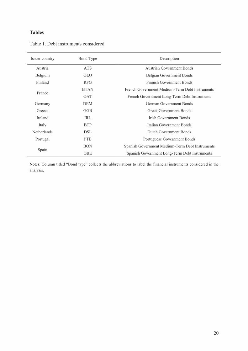
detailed description of the debt instruments considered in the analysis is presented in Table 1.

[Table 1]

For each trading day, the MTS Time series database reports the nominal value of

trading volume, the average size of trades, the last transaction price recorded before the

5:30pm Central European Time (CET) close, and the average best bid/ask spread throughout

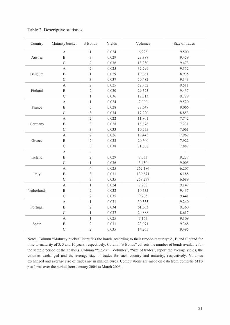
the trading day. Table 2 provides some descriptive statistics about average yields for each

country and maturity, the volume exchanged and the average size of trades. As expected, we

observe that yields increase monotonically with time-to-maturity without substantial

discrepancies in quoted bond yields for instruments with the same time-to-maturity. This

3 More in details bucket A includes all bonds maturing after the end of our estimation horizon with time-to-

maturity less than 3.3 years; bucket B includes all bonds with time-to-maturity between 4 and 6 years; bucket B

includes all bonds with time-to-maturity between 8.5 and 11 years.

4 Namely, Austria, Belgium, Finland, France, Germany, Greece, Ireland, Italy, Netherlands, Portugal and Spain.

Luxembourg is not included in the analysis since there is not any Luxembourgian bond quoted in MTS markets

in the sample period considered.

5 Benchmark bonds are defined as securities with an outstanding value of at least 5 billion euro that satisfy listing

requirements such as number of dealers acting as market makers.

6

suggests strong integration across euro-denominated government bonds within each bucket,

especially for those with shorter time-to-maturity. With more than 660 billion euros of

volumes exchanged over the period considered, Italy turns out to be by far the largest market,

whilst Irish government bonds are those with the smallest volume of exchanges (about 10

billion euros). Finally, the average size of trades presents some country patterns: for Italy and

Germany we report average sizes of trades (around 6-7 million euros) lower than the figures

(around 8-9 million euros) for the remaining countries.

[Table 2]

We supplement the MTS Time series database with the information extracted from

issuance calendars, which are a very powerful source of information to study government

bond markets and sovereign borrowers’ strategic behavior. In particular, we use issuance

calendars to shed light on the issuance frequencies of each country considered, the degree of

information disclosure related to different calendars and the presence of bunching in issuances,

namely a situation where two different countries issue a security with similar features in a

contemporaneous (same day) or nearly contemporaneous (the previous day or the following

day) way.6

A first evaluation of the data available from issuance calendar focuses on issuance

frequencies. Simple computations of the average numbers of issuances per month point out

how small borrowers (for instance Finland or Ireland) issue less frequently than large

borrowers (like Italy or France). As their financing and rolling over needs are rather limited in

absolute terms, they are required to issue in one shot a large share of their yearly needs so as

to entice investors immediately to relatively liquid issuances. For large countries, such a need

is less urgent; rather, they have to carefully smooth market issuances to avoid flooding the

market with so much paper that the cost of issuance is negatively affected by it.

6 For instance, between the 7th and the 8th of January 2004, Germany, France and Austria issued debt

instruments with the same time to maturity (ten years).

7

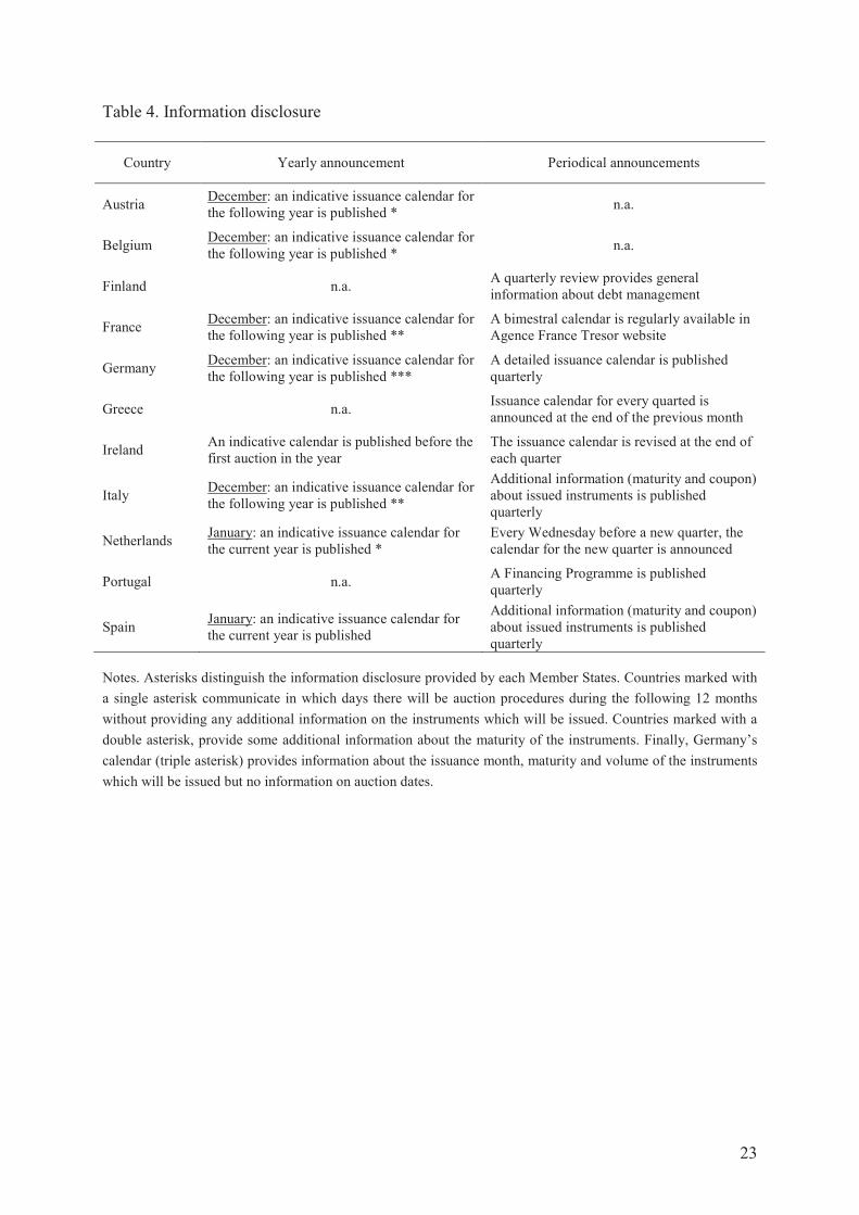
Furthermore, it appears that each country considered follows a certain pattern of

within-the-week issuances (Table 3). For example, Germany issues debt on Wednesday, while

France and Spain issue the first and the third Thursday of each month. Accuracy of issuance

calendar and the timing of their publication is a useful proxy to assess the degree of

information disclosure provided by each one of the countries considered. Publishing calendars

ahead of time and providing greater information to primary dealers may represent a

competitive advantage for sovereign borrowers with respect to competing issuers. Results of

this qualitative analysis show clearly that large borrowers provide a higher degree of

information disclosure (Table 4).

[Table 3]

[Table 4]

2.2 Variable construction

According to the approach described in Dufour and Skinner (2004), yields used in the

analysis are based on mid-quote prices, which are the prices collected from a quote at or

before 5pm CET having bid/ask spread within 3×Basis Point Value (BPV).7 If the spread is

beyond this limit, the mid-price is supposed to be non-representative. In other words, the

yields considered for each bond are based on the last valid best proposals before 5pm CET.

Following Biais et al. (2004), we computed a percentage spread ( s ) between the bond yield

( y ) and the 1-week Euribor rate ( e ) to control for exogenous changes in the general level of

interest rates: ( ) /s y e e= − .8

7 MTS data about daily prices refer to a quote at 5pm because the market provides a fixing at that time. The

choice looks appropriate. The lower trading intensity normally registered towards the end of the day should

imply a lower volatility. Besides, the market closes at 5:30pm and hence it seems reasonable to select a time

away from the closing time in order to avoid the effect of technical trading in the last few minutes before the

close.

8 Codogno et al. (2003) consider the difference between total yield differentials and relative asset swap spreads

to control for the exchange rate effect on yield differentials. The current paper does not compute this swap

8

Liquidity is proxied by the daily average bid/ask ( a ).9 Bid/ask spread measures the

tightness of the market, namely the distance between the transaction price and the mid-market

price for each bond considered. In the same way we described for yields, in order to exclude

non-tradable couples, the average bid/ask spread is computed using only observations having

bid/ask spread within 3×BPV. Since bid/ask spreads characterize market (il)liquidity, we

expect that wider bid/ask spreads translate into higher bond yields in order to compensate

higher transaction costs determined by illiquidity.

In keeping with the definition provided in Bagella et al. (2007), a bunching in issues

occurs when one country issues in the same day, in the previous day or in the following day

with respect to other countries issuances.10

Beside data on yields and liquidity, we thus

consider two bunching dummy variables 2B and 3B : the first dummy variable takes value 1 if

at least two countries issue together and 0 otherwise; the second dummy takes value 1 if at

least three countries issue together and 0 otherwise. This approach allows us to evaluate the

overall significance of the bunching effect and to assess the additional effect induced by

further sovereign borrowers’ (nearly) contemporaneous issuances.11

Note that it is crucial to distinguish between the issuance effect and the bunching

effect, both of which basically produce a similar impact in the bond market, possibly raising

differential because it considers term spreads (between long-term rates, s , and short-term rates, e ) in a post-

EMU period, when relative asset swaps coincide with yield differentials (Codogno et al., 2003).

9 Market depth data (bid and ask quantities and prices) were also considered in order to add robustness to the

analysis. However, this is not viable because the very high frequency of these data (tick-by-tick) is not consistent

with the daily frequency of the calendar data used to proxy bunching phenomena.

10 The estimation results presented in Section 3 below are robust with respect to the specification of the bunching

in issues: using a more restrictive definition of the bunching effect based on the contemporaneous issuances (that

is taking place in the same day), the results (not reported for the sake of brevity) are qualitatively similar to those

presented in the text. Results are available upon request.

11 In the context of the present work, we observe at most three countries bunching in issues, the number of

bunching dummy variables is not greater than two. Our strategy can be easily extended for the case of four or

more contemporaneous issuances.

9

yield spreads. The significance of these effects has different policy-making implications,

however. While potential inefficiencies due to issuance-overlapping can be avoided if

Member States agree to smooth the amount of paper totally issued weekly or monthly in the

primary market, the issuance effect reflects the impact of the choice of how often to issue on

the market, which is somehow constrained as a country naturally needs to finance its own

debt. In order to properly capture genuine bunching effects, we include a dummy variable c

tI

(*c

tI ), taking value 1 if there is a debt issuance for a given country (for the remaining EMU

countries) in a certain trading day and 0 otherwise, to control for the effect produced by a

(non) country-specific debt issuance in the primary market.

From an empirical perspective, a model which does not discern these two effects could

entail omitted variable problems: the issuance effect could be captured by the bunching

variable and the statistical significance of the effect given by contemporaneous issuances

could be biased. Moreover, the issuance dummy variable turns out to be useful to control for

additional interactions between primary and secondary government bond markets which do

not depend from bunching in issues, like the on-the-run/off-the-run effect or the switch

between first off-the-run and second off-the-run status (or more generally from a given order

of off-the-run-ness and the subsequent one).

3. Empirical analysis

3.1 The baseline model

We verify if (nearly) contemporaneous issuances by different euro-area Members States have

a significant impact on yield spreads, in the absence of coordination among sovereign

borrowers.12

To test this hypothesis, we present a simple model based on market

12

In the face of growing credit spreads differentials across euro-area issuers, the need for a European Debt

Management Agency as a form of coordination among Treasuries (firstly proposed by De Silguy in 1999) has

recently been advocated in the public debate.

10

microstructure variables, in the spirit of Codogno et al. (2003) and Biais et al. (2004), among

others. The overall impact of contemporaneous issuances on yield spreads is probably driven

by a set of different reasons (amount of debt issued, auction risks, hedging needs). For policy

reasons, we are interested in the global effect of bunching in issues. The aim of the present

paper is thus to test the significance of the bunching effect and the empirical model proposed

does not investigate its specific determinants.

Using the same notation as in Section 2.2 above, we estimate for each country and

each maturity bucket the following baseline model:

3*

2

c c c c c c c c c

jt jt t t k kt jt

k

s a I I B=

= + + + + + (1)

where the dependent variable, c

jts , is the percentage spread at time t for bond j issued by

country c ; c

jta denotes the daily average bid/ask spread for the same bond at time t ; tI and

*c

tI are dummy variables to control for debt issuances in the primary market; ktB ’s are

dummy variables to measure the bunching effect; finally, c

jtε is a mean zero process with

covariance matrix Σ , where Ω=Σ2

σ . The model is estimated by applying Generalized Least

Squares (GLS) with pooled time-series cross-sectional data. Since we consider separately

each country and each maturity bucket, we specified a common conditional mean across the

groups (bonds), with heterogeneity taking the form of different variances rather than shifts in

the means.13

3.2 Estimation results

13

Since all the countries considered publish in advance their issuance calendars (Table 4), the market knows in

advance when there will be a bunching in issues. As a consequence, the global bunching effect could be

underestimated since the model proposed is considering the effect produced in the bunching dates but it is not

taking into account the effect originated when calendars are published or the amounts to be issued are announced.

11

Estimation results for maturity bucket A (bonds with three years of time to maturity) are

presented in Table 5 - Panel A. When two countries issue together ( 2 1tB = ), the bunching of

issues tends to raise yield spreads. In other words, with two Member States issuing similar

bonds (in terms of time to maturity) at the same time, the cost of issuance for each sovereign

borrower is greater. When three countries issue together ( 3 1tB = ), yield spreads are even

higher for the majority of the countries considered. Overall, the bunching effect affects yield

spreads, with the marginal effect caused by an additional borrower issuing at the same time

being more intense. The effect of the country-specific issuance dummy, I , is non-negative

for large borrowers (Italy, France and Germany), whilst issuing short-term debt lowers yield

spreads for small borrowers. As for the dummy related to EMU partners’ issuances, *I , there

emerges a negligible role in explaining bond yields in all models (except for Belgium). The

liquidity effect, proxied by average bid/ask spread, is positive and significant in all entities of

reference, in a way consistent with the existent empirical literature. Finally, the adjusted 2R

statistics show quite high values for all the regressions.

Results obtained when considering maturity bucket B (bonds with five years of time to

maturity) confirm previous findings (Table 5 - Panel B). The bunching in issues caused by

two Member States leads to excess supply of similar securities lowering bond prices and

consequently increasing the yields offered. Further sovereign borrowers’ contemporaneous

issuances (that is when three countries issue together 5-year bonds) raise yields as well. The

country-specific issuance effect estimated for maturity bucket B is positive and statistically

significant in almost all cases. By contrast, the issuance of similar bonds from other EMU

countries tends to lower yields. Finally, the liquidity effect turns out to be positive and

significant at least at the 10 percent level for all the countries considered.

Estimation results for maturity bucket C (bonds with ten years of time to maturity)

shed further light on the overcrowding versus liquidity trade-off related to sovereign

12

borrowers’ contemporaneous issuances (Table 5 - Panel C). The coefficients for the bunching

variable are highly significant for the great majority of the countries considered, both when

considering the bunching effect provoked by two countries issuing together and when

considering the effect caused by an additional country bunching in issues. However, it is

interesting to focus on the sign of the relationships estimated. When two countries

contemporaneously issue the same kind of security, yield spreads are lower whereas a

bunching of issues raises yield spreads when there are three countries issuing at the same time

10-year bonds. This non-linear effect could be explained in the following way. When two

countries issue together 10-year bonds, the liquidity in secondary markets improves and the

yields offered are consequently lower. Note that this effect does not hold for shorter maturity

bonds (Panel A and B), which is consistent with the anecdotal evidence that long-term bonds

need higher amounts to be issued to reach liquidity. However, when there are three countries

issuing together 10-year bonds) the bunching effect changes sign and contemporaneous

issuances raise once again the cost of funding for sovereign borrowers.14

The country-specific

issuance effect is positive and statistically significant for the vast majority of models whilst

the effect of EMU partners’ issuances is mildly negative, as previously documented for the

case of 5-year bonds. Like for maturity bucket A and B, the liquidity effect is positive and

significant in almost all the countries considered.

[Table 5]

Overall, our results support the hypothesis that an excess supply of securities with

similar features force borrowers to offer higher yield spreads and imply that euro area public

debt managers could often gain by: a) credibly committing, through calendars of issuance, to

reach minimum sizes of issuance; b) credibly coordinating with other countries the proper

14

Our findings seem to suggest the existence of a sort of liquidity threshold. As the effect of debt issuance on

liquidity of the secondary market is not the focus of this paper, a detailed analysis on possible “liquidity

thresholds” could be the subject for further investigation.

13

strategy and timing of issuances so as to take advantage of smaller or larger issues of similar

instruments in the market at the same point in time.15

3.3 The impact of large and small borrowers’ issuances

Since the amount of debt issued each year by Italy is evidently larger than the amount issued

by small borrowers like Finland, one could wonder if contemporaneous issuances from large

borrowers (namely, France, Germany and Italy) could have a different impact with respect to

the bunching produced by small borrowers (the remainder of the countries considered). To

this aim, we re-consider the baseline model by estimating separately the following equation:

* * c c c c c c c Lc c Sc c L c S c

jt jt t t t t t jts a I I I B B= + + + + + + + (2)

where L

tB ( S

tB ) is the bunching dummy variable built by considering only large (small)

borrowers issuances belonging to the same maturity bucket of the j -th bond and where the

dummy *c

tI in (1) is split into two components related to large and small issuers ( *Lc

tI and

*Sc

tI , respectively).

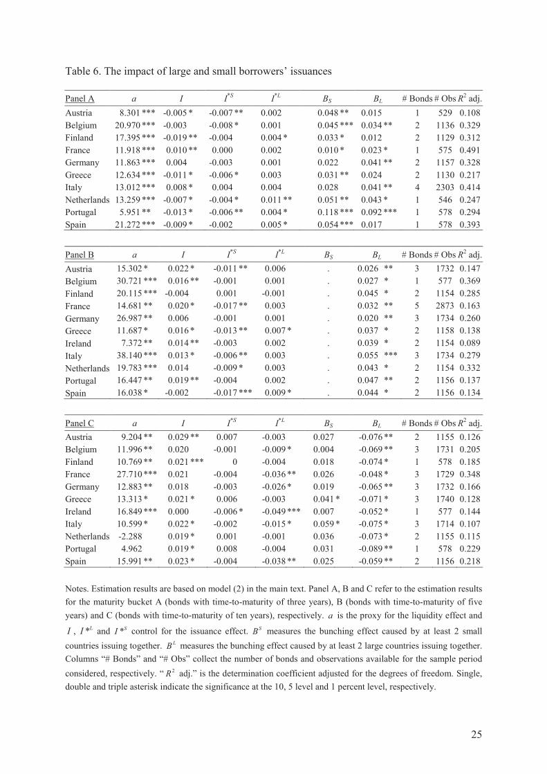
Results in Tables 6 document some differences between the bunching effect caused by

large borrowers and that one provoked by small borrowers’ contemporaneous issuances.

As for the maturity bucket including 3-year bonds (Table 6 - Panel A), estimation

results confirm previous findings when considering the bunching in issues: in general, the

(nearly) contemporaneous issuance of government paper of similar maturity significantly

increases yield spreads for the majority of the countries considered. This conclusion holds for

both small and large issuers. Evidence for the country-specific issuance dummies turns out to

be consistent with the results reported in Table 5 - Panel A. Note, however, that the scant

significant role for the *

tI variable for small borrowers can be partly attributed to the

asymmetric effect exerted by the *L

tI and *S

tI variables: while issuances of small borrowers

15

See Piga (1998) for a theoretical model carrying these implications.

14

lower the yields, the opposite finding emerges when considering the effect of the issuance

dummy *L

tI . Finally, coefficients estimated for the liquidity effect are generally positive and

statistically significant for all the countries, in a way consistent with the findings of the

baseline model.

With regard to bonds with 5 years of maturity, we observe that small borrowers are

never bunching in issues in the sample period considered. In particular, small borrowers issue

together but offering to the market bonds with different time-to-maturity. The aim of this

behavior is likely to be one of generating a euro yield curve capable of increasing the strategic

opportunities for traders and - hence - to raise the liquidity in the secondary markets (Bagella

et al., 2007). If we focus only on large borrowers issuances, estimation results support

previous considerations about the detrimental effect on yields spreads exerted by (nearly)

contemporaneous issuances: the amount of paper issued by two or three large borrowers

significantly raises yield spreads (see Table 6 - Panel B).

As regards the 10-year bond bucket (see Table 6 - Panel C), the overall effect of

issuances and bunching in issues for small borrowers is quite weak: we find indeed that both

*S

tI and S

tB have a negligible role in explaining yield spreads (except for Ireland, Greece and

Italy).16

Differently from what happens for the 5-year maturity bucket, however, yield spreads

are lower if large borrowers issues in isolation ( *L

tI ) or in a contemporaneous way ( L

tB ), as if

the amount of debt issued is still below a sort of liquidity threshold where overcrowding

replaces liquidity.17

This finding seems to confirm that those fixed income instruments seem

to have a higher capacity to absorb paper compared to instruments with shorter maturity.

16

Note that the positive sign associated with the S

tB variable could be the result of opposite effects related to the

bunching in issues of two small issuers (which lowers yields) and three small issuers (which raises yields), where

the latter tends to dominate the former, as previously documented in Table 5 - Panel C.

17 In our sample there are at most two large borrowers issuing 10-years government bonds.

15

More generally, our results underline that the significance of the bunching effect is

related to the degree of substitution across bonds. This is consistent with the evidence in

Pagano and Von Thadden (2004), according to which the degree of financial integration in

Europe appears to be inversely related to the maturity of the financial instruments.

Contemporaneous issuances exert indeed detrimental effects on yield spreads especially for

shorter-dated securities.

[Table 6]

4. Conclusions and further discussions

In an effort to contribute to the literature which considers how market microstructure might

influence government bond yields, this paper investigates on the liquidity versus

overcrowding trade-off related to sovereign borrowers’ issuances by testing for the

significance of a liquidity effect and a bunching effect due to (nearly) contemporaneous

issuances of bonds characterized by similar time-to-maturities. The role of broad and deep

primary and secondary Treasury bond markets in lowering the cost of borrowing for

governments’ financing needs is widely recognized. With issuance power still in the hands of

the different euro-area Member States, the growing financial integration in the EMU has

increased the competition between same-duration instruments due to their greater

substitutability.

Using daily data for a 27-month horizon (from January 2004 to March 2006), we find

a positive effect of bid/ask spreads on bond yields, therefore a negative relationship between

liquidity and yields offered, in a way consistent with the relevant literature. When considering

government bonds with three and five years of maturity, we show that the impact on yield

spreads of contemporaneous issuances of two or more countries is positive and strongly

significant, suggesting that an excess supply of similar securities tends to raise yield spreads.

As for securities with longer maturity, we document that the yields offered are lower when

16

two countries issuing together similar securities; in contrast, when three countries issue

together the bunching effect changes sign and contemporaneous issuances raise the costs of

funding for sovereign borrowers. The robustness of the findings obtained has been tested by

distinguishing between the bunching caused by large borrowers (Italy, France or Germany)

and the one due to small borrowers (the other EMU countries considered).

Our results document that the significance of the bunching effect is related to the

degree of substitution across bonds: contemporaneous issuances exert indeed a detrimental

effect on yield spreads especially for shorter-dated securities. Our findings have relevant

implications for policy managers attempting to identify conditions likely to enhance liquidity

in the secondary market for government bonds in Europe. To the extent that yield spreads

depend on bunching in issues, agreement between sovereign borrowers on dates and

frequency of debt issuances could significantly lower the costs of funding for Member States.

This does not necessarily imply to switch to the establishment of a single-issuer of debt

responsible for issuing some part of euro-zone government bonds, as long ago suggested by

de Silguy (1999). Our results should inform instead that greater co-ordination in debt issuance

suggest scope for efficiency gains. These improvements in efficiency should gain even more

relevance in the light of the ongoing financial turmoil since the dramatic increase in the

supply of government paper (due to the soaring costs of financial support schemes and other

crisis-related expenditures as well as recession-induced falls in tax income and an increase in

recession-related expenditures) has worsened issuance conditions and inflamed liquidity

pressures in secondary markets (Blommestein, 2009). More generally, the optimization of

issuing procedures in terms of dates and frequency of debt issuances is a relevant topic not

only for the market of euro-denominated government securities but also for other financial

markets. In this respect, our conclusions about the gains from coordination between issuance

17

plans to mitigate liquidity problems may be of interest for a number of policy managers and

market regulators.

18

References

Bagella, M., Coppola, A., Pacini, R. and Piga, G., Euro debt primary market report, Global

Research, UniCredit Markets & Investment Banking, 2007.

Bernoth, K., von Hagen, J. and Schuhknecht, L., ‘Sovereign risk premia in the European

government bond market’, Working Paper (ECB, 2004).

Biais, B., Renucci, A. and Saint-Paul, G., ‘Liquidity and the cost of funds in the European

treasury bill market’, Working Paper (IDEI, 2004).

Blommestein, H.J. ‘New challenges in the use of government debt issuance procedures,

techniques and policies in OECD markets’, OECD Financial Market Trends, Vol. 1,

2009, pp. 1-12.

Caporale, G.M. and Girardi, A., ‘Price formation on the EuroMTS platform’, Applied

Economics Letters, Vol. 18, 2011, pp. 229-33.

Codogno, L., Favero, C. and Missale, A., ‘Government bond spreads’, Economic Policy, Vol.

18, 2003, pp. 503-32.

Coppola, A. and Pacini, R., ‘Il mercato primario dei titoli di Stato: procedure europee a

confronto’, in Bagella, M., ed., Rapporto sul Sistema Finanziario Italiano (Rome:

Aracne Editrice, 2006), pp. 9-49.

De Silguy, Y.T., ‘The euro: the key to Europe’s lasting success in the global economy’,

speech given at the Corporation of London, July 26 1999.

Dufour, A. and Skinner, F., ‘MTS time series’, Working Paper (University of Reading, 2004).

European Commission, Co-ordinated public debt issuance in the Euro area, Brussels, 2000.

Favero, C., Missale, A. and Piga, G., ‘EMU and public debt management: one money, one

debt?’, Policy Report (CEPR, 1999).

Favero, C., Pagano, M. and von Thadden, E., ‘Valuation, liquidity, and risk in government

bond markets’, Working Paper (Bocconi University, 2005).

19

Galati, G. and Tsatsaronis, K., ‘The impact of the euro on Europe’s financial markets’,

Financial Markets, Institutions and Instruments, Vol. 12, 2003, pp. 165-221.

Hund, J. and Lesmond, D.A., ‘Liquidity and credit risk in emerging debt markets’, Working

Paper (Tulane University, 2008).

Keloharju, M., Malkamäki, M., Nyborg, K.G. and Rydqvist K., ‘A descriptive analysis of the

Finnish treasury bond market 1991–1999’, Working Paper (Bank of Finland Research

Discussion Papers 6/2002, 2002).

Mizrach, B. ‘Jump and cojump risk in subprime home equity derivatives’, Working Paper

(Rutgers University, 2008).

Newman, Y. and Rierson, M., ‘Illiquidity spillovers: theory and evidence from European

telecom bond issuance", Mimeo (Stanford University, 2004).

Norden, L. and Weber, M., ‘The comovement of credit default swap, bond and stock markets:

an empirical analysis’, European Financial Management, Vol. 15, 2009, pp. 529-62.

Pagano, M. and Von Thadden, E.L., ‘The European bond markets under EMU’, Oxford

Review of Economic Policy, Vol. 20, 2004, pp. 531-54.

Persaud, A.D., ‘Improving efficiency in the European government bond market’, Working

Paper (ICAP plc., 2006).

Piga, G., ‘In search of an independent province for the treasuries: how should public debt be

managed?’, Journal of Economics and Business, Vol. 50, 1998, pp. 257-75.

Poterba, J.M. and Reuben, K.S., ‘Fiscal news, state budget rules, and tax-exempt bond yields’,

Journal of Urban Economics, Vol. 50, 2001, pp. 537-62.

Schuknecht L., J. von Hagen and G. Wolswijk (2011), Government bond risk premiums in the

EU revisited: the impact of the financial crisis, European Journal of Political Economy,

27: 36-43.

20

Tables

Table 1. Debt instruments considered

Issuer country Bond Type Description

Austria ATS Austrian Government Bonds

Belgium OLO Belgian Government Bonds

Finland RFG Finnish Government Bonds

France BTAN French Government Medium-Term Debt Instruments

OAT French Government Long-Term Debt Instruments

Germany DEM German Government Bonds

Greece GGB Greek Government Bonds

Ireland IRL Irish Government Bonds

Italy BTP Italian Government Bonds

Netherlands DSL Dutch Government Bonds

Portugal PTE Portuguese Government Bonds

Spain BON Spanish Government Medium-Term Debt Instruments

OBE Spanish Government Long-Term Debt Instruments

Notes. Column titled “Bond type” collects the abbreviations to label the financial instruments considered in the

analysis.

21

Table 2. Descriptive statistics

Country Maturity bucket # Bonds Yields Volumes Size of trades

Austria

A 1 0.024 6,228 9.500

B 3 0.029 23,887 9.459

C 2 0.036 13,230 9.473

Belgium

A 2 0.025 32,799 9.152

B 1 0.029 19,061 8.935

C 3 0.037 50,482 9.143

Finland

A 2 0.025 52,952 9.511

B 2 0.030 29,525 9.437

C 1 0.036 17,313 9.729

France

A 1 0.024 7,000 9.520

B 5 0.028 38,647 9.066

C 3 0.034 17,220 8.853

Germany

A 2 0.022 11,801 7.742

B 3 0.028 18,876 7.231

C 3 0.033 10,775 7.061

Greece

A 2 0.026 19,445 7.962

B 2 0.033 20,600 7.922

C 3 0.038 71,808 7.887

Ireland

A . . . .

B 2 0.029 7,033 9.237

C 1 0.036 3,450 9.005

Italy

A 4 0.025 262,186 6.207

B 3 0.031 139,871 6.188

C 3 0.035 258,277 6.689

Netherlands

A 1 0.024 7,288 9.147

B 2 0.032 10,535 9.437

C 2 0.035 9,705 9.441

Portugal

A 1 0.031 30,535 9.240

B 2 0.034 61,663 9.360

C 1 0.037 24,888 8.617

Spain

A 1 0.025 7,163 9.109

B 2 0.031 23,071 9.368

C 2 0.035 14,265 9.495

Notes. Column “Maturity bucket” identifies the bonds according to their time-to-maturity: A, B and C stand for

time-to-maturity of 3, 5 and 10 years, respectively. Column “# Bonds” collects the number of bonds available for

the sample period of the analysis. Column “Yields”, “Volumes”, “Size of trades”, report the average yields, the

volumes exchanged and the average size of trades for each country and maturity, respectively. Volumes

exchanged and average size of trades are in million euros. Computations are made on data from domestic MTS

platforms over the period from January 2004 to March 2006.

22

Table 3. Issuances patterns

Country Day of the week

Mon-1 Tue-1 Wed-1 Thu-1 Fri-1 Mon-2 Tue-2 Wed-2 Thu-2 Fri-2

Austria ATSs

Belgium

Finland

France OATs

Germany DEMs

Greece GGBs

Ireland

Italy BTPs

Netherlands DSLs

Portugal PTEs

Spain BONs

Country Day of the week

Mon-3 Tue-3 Wed-3 Thu-3 Fri-3 Mon-4 Tue-4 Wed-4 Thu-4 Fri-4

Austria

Belgium OLOs

Finland

France BTANs

Germany DEMs DEMs

Greece

Ireland IRLs

Italy BTPs BTPs

Netherlands

Portugal

Spain OBEs

Notes. Columns identify the day of the week in which the different debt instruments (bond types) are usually

issued according to the patterns identified over the sample period considered. For example, Mon-2 stands for the

second Monday of the month while Fri-4 stands for the fourth Friday of the month. Bond types are described in

Table 1.

23

Table 4. Information disclosure

Country Yearly announcement Periodical announcements

Austria December: an indicative issuance calendar for

the following year is published * n.a.

Belgium December: an indicative issuance calendar for

the following year is published * n.a.

Finland n.a. A quarterly review provides general

information about debt management

France December: an indicative issuance calendar for

the following year is published **

A bimestral calendar is regularly available in

Agence France Tresor website

Germany December: an indicative issuance calendar for

the following year is published ***

A detailed issuance calendar is published

quarterly

Greece n.a. Issuance calendar for every quarted is

announced at the end of the previous month

Ireland An indicative calendar is published before the

first auction in the year

The issuance calendar is revised at the end of

each quarter

Italy December: an indicative issuance calendar for

the following year is published **

Additional information (maturity and coupon)

about issued instruments is published

quarterly

Netherlands January: an indicative issuance calendar for

the current year is published *

Every Wednesday before a new quarter, the

calendar for the new quarter is announced

Portugal n.a. A Financing Programme is published

quarterly

Spain January: an indicative issuance calendar for

the current year is published

Additional information (maturity and coupon)

about issued instruments is published

quarterly

Notes. Asterisks distinguish the information disclosure provided by each Member States. Countries marked with

a single asterisk communicate in which days there will be auction procedures during the following 12 months

without providing any additional information on the instruments which will be issued. Countries marked with a

double asterisk, provide some additional information about the maturity of the instruments. Finally, Germany’s

calendar (triple asterisk) provides information about the issuance month, maturity and volume of the instruments

which will be issued but no information on auction dates.

24

Table 5. Baseline estimation results

Panel A a I *I 2B

3B # Bonds # Obs 2R adj.

Austria 8.242 * -0.009 ** -0.003 0.010 * 0.031 * 1 529 0.099

Belgium 21.941 *** -0.004 -0.005 * 0.021 ** 0.011 2 1136 0.308

Finland 17.471 *** -0.009 * -0.002 0.019 * 0.038 ** 2 1129 0.291

France 11.880 *** 0.011 *** 0.000 0.004 0.018 * 1 575 0.489

Germany 11.703 *** 0.002 -0.001 0.009 * 0.031 * 2 1157 0.323

Greece 12.714 * -0.015 *** -0.001 0.003 0.046 ** 2 1130 0.174

Italy 13.997 *** 0.003 0.005 0.006 * 0.013 ** 4 2303 0.410

Netherlands 13.409 ** -0.012 ** 0.002 0.013 * 0.027 * 1 546 0.184

Portugal 6.684 * -0.007 * 0.000 0.001 0.014 1 578 0.283

Spain 21.385 *** -0.017 ** 0.001 0.008 * 0.032 ** 1 578 0.382

Panel B a I *I 2B

3B # Bonds # Obs 2R adj.

Austria 15.823 * 0.023 * -0.008 * 0.014 * 0.046 ** 3 1732 0.148

Belgium 32.237 *** 0.018 ** -0.001 0.013 ** 0.010 * 1 577 0.375

Finland 21.423 *** -0.005 0.001 0.027 *** 0.039 * 2 1154 0.293

France 14.745 ** 0.021 * -0.012 * 0.010 0.048 ** 5 2873 0.169

Germany 26.337 ** 0.007 *** -0.001 0.016 ** 0.013 3 1734 0.273

Greece 6.245 * 0.021 * -0.009 * 0.021 *** 0.066 *** 2 1158 0.146

Ireland 18.378 ** 0.015 ** -0.002 0.021 0.042 * 2 1154 0.095

Italy 38.306 *** 0.018 * -0.004 * 0.018 * 0.062 *** 3 1734 0.301

Netherlands 19.585 *** 0.021 *** -0.006 0.032 *** 0.054 *** 2 1154 0.362

Portugal 16.760 ** 0.020 ** -0.004 0.040 ** 0.007 2 1156 0.151

Spain 16.830 * -0.004 -0.012 ** 0.018 * 0.037 ** 2 1156 0.149

Panel C a I *I 2B

3B # Bonds # Obs 2R adj.

Austria 9.343 ** 0.030 ** 0.006 -0.069 *** 0.112 ** 2 1155 0.130

Belgium 11.730 ** 0.037 * -0.004 -0.032 *** 0.083 3 1731 0.212

Finland 11.096 ** 0.023 *** -0.002 -0.056 ** 0.091 ** 1 578 0.192

France 26.694 *** 0.042 ** -0.017 * -0.013 * 0.077 ** 3 1729 0.362

Germany 12.318 ** 0.033 ** -0.012 -0.030 *** 0.065 * 3 1732 0.173

Greece 14.028 ** 0.031 * 0.005 -0.059 ** 0.104 ** 3 1740 0.134

Ireland 15.871 *** 0.003 -0.024 ** -0.030 * 0.114 1 577 0.151

Italy 11.336 * 0.035 ** -0.007 * -0.033 ** 0.113 ** 3 1714 0.112

Netherlands -2.466 0.027 *** 0.001 -0.080 *** 0.126 *** 2 1155 0.121

Portugal 5.387 * 0.023 * 0.007 -0.041 * 0.148 *** 1 578 0.242

Spain 14.620 ** 0.041 ** -0.018 * -0.027 * 0.085 ** 2 1156 0.231

Notes. Estimation results are based on model (1) in the main text. Panel A, B and C refer to the estimation results

for the maturity bucket A (bonds with time-to-maturity of three years), B (bonds with time-to-maturity of five

years) and C (bonds with time-to-maturity of ten years), respectively. a is the proxy for the liquidity effect and

I and *I control for the issuance effect. 2

B measures the bunching effect caused by 2 countries issuing

together. 3

B measures the additional effect of a third country bunching in issues. Columns “# Bonds” and “#

Obs” collect the number of bonds and observations available for the sample period considered, respectively.

“ 2R adj.” is the determination coefficient adjusted for the degrees of freedom. Single, double and triple asterisk

indicate the significance at the 10, 5 level and 1 percent level, respectively.

25

Table 6. The impact of large and small borrowers’ issuances

Panel A a I I*S

I*L

BS BL # Bonds # Obs R2 adj.

Austria 8.301 *** -0.005 * -0.007 ** 0.002 0.048 ** 0.015 1 529 0.108

Belgium 20.970 *** -0.003 -0.008 * 0.001 0.045 *** 0.034 ** 2 1136 0.329

Finland 17.395 *** -0.019 ** -0.004 0.004 * 0.033 * 0.012 2 1129 0.312

France 11.918 *** 0.010 ** 0.000 0.002 0.010 * 0.023 * 1 575 0.491

Germany 11.863 *** 0.004 -0.003 0.001 0.022 0.041 ** 2 1157 0.328

Greece 12.634 *** -0.011 * -0.006 * 0.003 0.031 ** 0.024 2 1130 0.217

Italy 13.012 *** 0.008 * 0.004 0.004 0.028 0.041 ** 4 2303 0.414

Netherlands 13.259 *** -0.007 * -0.004 * 0.011 ** 0.051 ** 0.043 * 1 546 0.247

Portugal 5.951 ** -0.013 * -0.006 ** 0.004 * 0.118 *** 0.092 *** 1 578 0.294

Spain 21.272 *** -0.009 * -0.002 0.005 * 0.054 *** 0.017 1 578 0.393

Panel B a I I*S

I*L

BS BL # Bonds # Obs R2 adj.

Austria 15.302 * 0.022 * -0.011 ** 0.006 . 0.026 ** 3 1732 0.147

Belgium 30.721 *** 0.016 ** -0.001 0.001 . 0.027 * 1 577 0.369

Finland 20.115 *** -0.004 0.001 -0.001 . 0.045 * 2 1154 0.285

France 14.681 ** 0.020 * -0.017 ** 0.003 . 0.032 ** 5 2873 0.163

Germany 26.987 ** 0.006 -0.001 0.001 . 0.020 ** 3 1734 0.260

Greece 11.687 * 0.016 * -0.013 ** 0.007 * . 0.037 * 2 1158 0.138

Ireland 7.372 ** 0.014 ** -0.003 0.002 . 0.039 * 2 1154 0.089

Italy 38.140 *** 0.013 * -0.006 ** 0.003 . 0.055 *** 3 1734 0.279

Netherlands 19.783 *** 0.014 -0.009 * 0.003 . 0.043 * 2 1154 0.332

Portugal 16.447 ** 0.019 ** -0.004 0.002 . 0.047 ** 2 1156 0.137

Spain 16.038 * -0.002 -0.017 *** 0.009 * . 0.044 * 2 1156 0.134

Panel C a I I*S

I*L

BS BL # Bonds # Obs R2 adj.

Austria 9.204 ** 0.029 ** 0.007 -0.003 0.027 -0.076 ** 2 1155 0.126

Belgium 11.996 ** 0.020 -0.001 -0.009 * 0.004 -0.069 ** 3 1731 0.205

Finland 10.769 ** 0.021 *** 0 -0.004 0.018 -0.074 * 1 578 0.185

France 27.710 *** 0.021 -0.004 -0.036 ** 0.026 -0.048 * 3 1729 0.348

Germany 12.883 ** 0.018 -0.003 -0.026 * 0.019 -0.065 ** 3 1732 0.166

Greece 13.313 * 0.021 * 0.006 -0.003 0.041 * -0.071 * 3 1740 0.128

Ireland 16.849 *** 0.000 -0.006 * -0.049 *** 0.007 -0.052 * 1 577 0.144

Italy 10.599 * 0.022 * -0.002 -0.015 * 0.059 * -0.075 * 3 1714 0.107

Netherlands -2.288 0.019 * 0.001 -0.001 0.036 -0.073 * 2 1155 0.115

Portugal 4.962 0.019 * 0.008 -0.004 0.031 -0.089 ** 1 578 0.229

Spain 15.991 ** 0.023 * -0.004 -0.038 ** 0.025 -0.059 ** 2 1156 0.218

Notes. Estimation results are based on model (2) in the main text. Panel A, B and C refer to the estimation results

for the maturity bucket A (bonds with time-to-maturity of three years), B (bonds with time-to-maturity of five

years) and C (bonds with time-to-maturity of ten years), respectively. a is the proxy for the liquidity effect and

I , *LI and *SI control for the issuance effect. SB measures the bunching effect caused by at least 2 small

countries issuing together. LB measures the bunching effect caused by at least 2 large countries issuing together.

Columns “# Bonds” and “# Obs” collect the number of bonds and observations available for the sample period

considered, respectively. “ 2R adj.” is the determination coefficient adjusted for the degrees of freedom. Single,

double and triple asterisk indicate the significance at the 10, 5 level and 1 percent level, respectively.