arXiv:0805.1629v2 [stat.ME] 13 May 2008 Technical Report # KU-EC-08-1: Overall and Pairwise Segregation Tests Based on Nearest Neighbor Contingency Tables Elvan Ceyhan * May 13, 2008 Abstract Multivariate interaction between two or more classes (or species) has important consequences in many fields and causes multivariate clustering patterns such as segregation or association. The spatial segregation occurs when members of a class tend to be found near members of the same class (i.e., near conspecifics) while spatial association occurs when members of a class tend to be found near members of the other class or classes. These patterns can be studied using a nearest neighbor contingency table (NNCT). The null hypothesis is randomness in the nearest neighbor (NN) structure, which may result from — among other patterns — random labeling (RL) or complete spatial randomness (CSR) of points from two or more classes (which is called the CSR independence, henceforth). In this article, we introduce new versions of overall and cell-specific tests based on NNCTs (i.e., NNCT-tests) and compare them with Dixon’s overall and cell-specific tests. These NNCT-tests provide information on the spatial interaction between the classes at small scales (i.e., around the average NN distances between the points). Overall tests are used to detect any deviation from the null case, while the cell-specific tests are post hoc pairwise spatial interaction tests that are applied when the overall test yields a significant result. We analyze the distributional properties of these tests; assess the finite sample performance of the tests by an extensive Monte Carlo simulation study. Furthermore, we show that the new NNCT-tests have better performance in terms of Type I error and power. We also illustrate these NNCT-tests on two real life data sets. Keywords: Association; clustering; completely mapped data; complete spatial randomness; random labeling; spatial pattern ∗ corresponding author. e-mail: [email protected] (E. Ceyhan) ∗ Department of Mathematics, Ko¸ c University, Sarıyer, 34450, Istanbul, Turkey. 1

Welcome message from author
This document is posted to help you gain knowledge. Please leave a comment to let me know what you think about it! Share it to your friends and learn new things together.
Transcript

arX
iv:0
805.
1629
v2 [
stat
.ME
] 1
3 M
ay 2
008
Technical Report # KU-EC-08-1:
Overall and Pairwise Segregation Tests Based on Nearest Neighbor
Contingency Tables
Elvan Ceyhan ∗
May 13, 2008
Abstract
Multivariate interaction between two or more classes (or species) has important consequences in manyfields and causes multivariate clustering patterns such as segregation or association. The spatial segregationoccurs when members of a class tend to be found near members of the same class (i.e., near conspecifics)while spatial association occurs when members of a class tend to be found near members of the other classor classes. These patterns can be studied using a nearest neighbor contingency table (NNCT). The nullhypothesis is randomness in the nearest neighbor (NN) structure, which may result from — among otherpatterns — random labeling (RL) or complete spatial randomness (CSR) of points from two or more classes(which is called the CSR independence, henceforth). In this article, we introduce new versions of overalland cell-specific tests based on NNCTs (i.e., NNCT-tests) and compare them with Dixon’s overall andcell-specific tests. These NNCT-tests provide information on the spatial interaction between the classes atsmall scales (i.e., around the average NN distances between the points). Overall tests are used to detectany deviation from the null case, while the cell-specific tests are post hoc pairwise spatial interaction teststhat are applied when the overall test yields a significant result. We analyze the distributional propertiesof these tests; assess the finite sample performance of the tests by an extensive Monte Carlo simulationstudy. Furthermore, we show that the new NNCT-tests have better performance in terms of Type I errorand power. We also illustrate these NNCT-tests on two real life data sets.
Keywords: Association; clustering; completely mapped data; complete spatial randomness; random labeling; spatialpattern
∗corresponding author.
e-mail: [email protected] (E. Ceyhan)
∗Department of Mathematics, Koc University, Sarıyer, 34450, Istanbul, Turkey.
1

1 Introduction
Multivariate clustering patterns such as segregation or association. result from multivariate interaction be-tween two or more classes (or species). Such patterns are of interest in ecological sciences and other applicationareas. See, for example, Pielou (1961), Whipple (1980), and Dixon (1994, 2002). For convenience and gen-erality, we refer to the different types of points as “classes”, but the class can stand for any characteristic ofan observation at a particular location. For example, the spatial segregation pattern has been investigatedfor species (Diggle (2003)), age classes of plants (Hamill and Wright (1986)), fish species (Herler and Patzner(2005)), and sexes of dioecious plants (Nanami et al. (1999)). Many of the epidemiological applications arefor a two-class system of case and control labels (Waller and Gotway (2004)). These methods can also beapplied to social and ethnic segregation of residential areas. For simplicity, we discuss the spatial interactionbetween two and three classes only; the extension to the case with more classes is straightforward. Thenull pattern is usually one of the two (random) pattern types: random labeling (RL) or complete spatialrandomness (CSR). We consider two major types of spatial clustering patterns as alternatives: segregationand association. Segregation (association) occurs when objects of a given class have NNs that are more (less)frequently of the same (other) class than would be expected if there were randomness in the NN structure.
In statistical and other literature, many univariate and multivariate spatial clustering tests have beenproposed (Kulldorff (2006)). These include comparison of Ripley’s K(t) and L(t) functions (Ripley (2004)),comparison of nearest neighbor (NN) distances (Cuzick and Edwards (1990), Diggle (2003)), and analysisof nearest neighbor contingency tables (NNCTs) which are constructed using the NN frequencies of classes(Pielou (1961), Meagher and Burdick (1980)). Pielou (1961) proposed various tests and Dixon (1994) intro-duced an overall test of segregation, cell-specific and class-specific tests based on NNCTs in a two-class settingand extended his tests to multi-class case in (Dixon (2002)).
In this article, we introduce new overall and cell-specific tests of segregation based on NNCTs for testingspatial clustering patterns in a multi-class setting. We compare these tests with Dixon’s NNCT-tests whichare introduced for testing against the RL of points (Dixon (1994)). We extend the use of these tests forthe CSR independence pattern also. We also compare the NNCT-tests with Ripley’s K or L-functions andpair correlation function g(t) (Stoyan and Stoyan (1994)), which are methods for second-order analysis of thepoint pattern. We only consider completely mapped data; i.e., for our data sets, the locations of all events ina defined area are observed. We show through simulation that Dixon’s cell-specific test can have undesirableproperties in some situations. The newly proposed cell-specific tests perform better (in terms of empirical sizeand power) than Dixon’s cell-specific tests. Likewise the new overall test tends to have higher power comparedto Dixon’s overall test under segregation of the classes. Furthermore, we demonstrate that NNCT-tests andRipley’s L-function (and related methods) answer different questions about the pattern of interest.
We provide the null and alternative patterns in Section 2, describe the NNCTs in Section 3, provide thecell-specific tests in Section 4, overall tests in Section 5, empirical significance levels in the two- and three-class cases in Sections 6.1 and 7.1, respectively, rejection rates of the tests under various Poisson processesin Section 8, empirical power comparisons under the segregation and association alternatives in the two-classcase in Section 9, in the three-class case in Section 10, examples in Section 11, and our conclusions andguidelines for using the tests in Section 12.
2 Null and Alternative Patterns
In this section, for simplicity, we describe the spatial point patterns for two classes only; the extension tomulti-class case is straightforward.
In the univariate spatial point pattern analysis, the null hypothesis is usually complete spatial randomness(CSR) (Diggle (2003)). Given a spatial point pattern P = {Xi(D), i = 1, . . . , n : D ⊂ R
2} where Xi(D) isthe Bernoulli random variable denoting the event that point i is in region D. The pattern P exhibits CSR ifgiven n events in domain D, the events are an independent random sample from a uniform distribution onD. This implies there is no spatial interaction, i.e., the locations of these points have no influence on oneanother. Furthermore, when the reference region D is large, the number of points in any planar region witharea A(D) follows (approximately) a Poisson distribution with intensity λ and mean λ · A(D).
2

To investigate the spatial interaction between two or more classes in a multivariate process, usually thereare two benchmark hypotheses: (i) independence, which implies two classes of points are generated by a pairof independent univariate processes and (ii) random labeling (RL), which implies that the class labels arerandomly assigned to a given set of locations in the region of interest (Diggle (2003)). In this article, we willconsider two random pattern types as our null hypotheses: CSR of points from two classes (this pattern willbe called the CSR independence, henceforth) or RL. In the CSR independence pattern, points from each ofthe two classes independently satisfy the CSR pattern in the region of interest. On the other hand, randomlabeling (RL) is the pattern in which, given a fixed set of points in a region, class labels are assigned to thesefixed points randomly so that the labels are independent of the locations. So RL is less restrictive than CSRindependence. CSR independence is a process defining the spatial distribution of event locations, while RLis a process, conditioned on locations, defining the distribution of labels on these locations.
Our null hypothesis isHo : randomness in the NN structure.
Although RL and CSR independence are not same, they lead to the same null model in tests using NNCT,which does not require spatially-explicit information. That is, when the points from two classes are assumedto be independently uniformly distributed over the region of interest, i.e., under the CSR independencepattern, or when only the labeling (or marking) of a set of fixed points, where the allocation of the pointsmight be regular, aggregated, or clustered, or of lattice type, is considered, i.e., under the RL pattern, thereis randomness in the NN structure. The distinction between RL and CSR independence is very importantwhen defining the appropriate null model in practice, i.e., the null model depends on the particular ecologicalcontext. Goreaud and Pelissier (2003) state that CSR independence implies that the two classes are a priorithe result of different processes (e.g., individuals of different species or age cohorts), whereas RL impliesthat some processes affect a posteriori the individuals of a single population (e.g., diseased vs. non-diseasedindividuals of a single species). We provide the differences in the proposed tests under these two patterns.
We treat CSR independence or RL as the main null model of interest, since this is the logical point ofdeparture (Diggle (2003)). However, in the ecological and epidemiological settings, CSR independence is theexception rather than rule. Furthermore, it is conceivable for other models to imply randomness in the NNstructure also. We also consider patterns that deviate from stationarity or homogeneity in the point process.In particular, we consider various types of Poisson cluster processes (Diggle (2003)) and other inhomogeneousPoisson processes (Baddeley and Turner (2005)). Randomness in the NN structure will hold if both classesindependently follow the same process with points having the same support. For example, in a Poisson clusterprocess, NN structure will be random if parents are the same for each class. If classes have different parentsets, then the Poisson cluster process will imply segregation of the classes. If parent and offspring sets aretreated as two different classes, then Poisson cluster process will imply association of the two classes. Further,if the two classes are from the same inhomogeneous Poisson pattern, again randomness in the NN structurewill follow. But when the two classes follow different inhomogeneous Poisson patterns whose point intensitiesdiffer in space, it might imply the segregation or association of the classes.
As clustering alternatives, we consider two major types of spatial patterns: segregation and association.Segregation occurs if the NN of an individual is more likely to be of the same class as the individual than tobe from a different class; i.e., the members of the same class tend to be clumped or clustered (see, e.g., Pielou(1961)). For instance, one type of plant might not grow well around another type of plant and vice versa. Inplant biology, one class of points might represent the coordinates of trees from a species with large canopy,so that other plants (whose coordinates are the other class of points) that need light cannot grow (well or atall) around these trees. See, for instance, (Dixon (1994); Coomes et al. (1999)).
Association occurs if the NN of an individual is more likely to be from another class than to be of thesame class as the individual. For example, in plant biology, the two classes of points might represent thecoordinates of mutualistic plant species, so the species depend on each other to survive. As another example,one class of points might be the geometric coordinates of parasitic plants exploiting the other plant whosecoordinates are of the other class. In epidemiology, one class of points might be the geographical coordinatesof residences of cases and the other class of points might be the coordinates of the residences of controls.
Each of the two patterns of segregation and association are not symmetric in the sense that, when twoclasses are segregated (or associated), they do not necessarily exhibit the same degree of segregation (orassociation). For example, when points from each of two classes labeled as X and Y are clustered at differentlocations, but class X is loosely clustered (i.e., its point intensity in the clusters is smaller) compared to class
3

Y . So classes X and Y are segregated but class Y is more segregated than class X . Similarly, when class Ypoints are clustered around class X points but not vice versa, classes Y and X are associated, but class Y ismore associated with class X compared to the other way around. Many different forms of segregation (andassociation) are possible. Although it is not possible to list all segregation types, its existence can be testedby an analysis of the NN relationships between the classes (Pielou (1961)).
3 Nearest Neighbor Contingency Tables
NNCTs are constructed using the NN frequencies of classes. We describe the construction of NNCTs fortwo classes; extension to multi-class case is straightforward. Consider two classes with labels {1, 2}. Let Ni
be the number of points from class i for i ∈ {1, 2} and n be the total sample size, so n = N1 + N2. If werecord the class of each point and the class of its NN, the NN relationships fall into four distinct categories:(1, 1), (1, 2); (2, 1), (2, 2) where in cell (i, j), class i is the base class, while class j is the class of its NN.That is, the n points constitute n (base, NN) pairs. Then each pair can be categorized with respect to thebase label (row categories) and NN label (column categories). Denoting Nij as the frequency of cell (i, j)for i, j ∈ {1, 2}, we obtain the NNCT in Table 1 where Cj is the sum of column j; i.e., number of timesclass j points serve as NNs for j ∈ {1, 2}. Furthermore, Nij is the cell count for cell (i, j) that is the count
of all (base, NN) pairs each of which has label (i, j). Note also that n =∑
i,j Nij ; ni =∑2
j=1 Nij ; and
Cj =∑2
i=1 Nij . By construction, if Nij is larger than expected, then class j serves as NN more frequently toclass i than expected, which implies segregation if i = j and association of class j with class i if i 6= j. On theother hand, if Nij is smaller than expected, then class j serves as NN less frequently to class i than expected,which implies lack of segregation if i = j and lack of association of class j with class i if i 6= j. Furthermore,we adopt the convention that variables denoted by upper case letters are random quantities, while variablesdenoted by lower case letters fixed quantities. Hence, column sums and cell counts are random, while rowsums and the overall sum are fixed quantities in a NNCT.
NN classclass 1 class 2 sum
class 1 N11 N12 n1base classclass 2 N21 N22 n2
sum C1 C2 n
Table 1: The NNCT for two classes.
Pielou (1961) used Pearson’s χ2 test of independence for testing segregation. Due to the ease in com-putation and interpretation, Pielou’s test of segregation is used frequently (Meagher and Burdick (1980))for both completely mapped and sparsely sampled data. For example, Pielou’s test is used for the segre-gation between males and females in dioecious species (see, e.g., Herrera (1988) and Armstrong and Irvine(1989)) and between different species (Good and Whipple (1982)). However Pielou’s test is not appropriatefor completely mapped data (Meagher and Burdick (1980), Dixon (1994)), since the χ2 test of independencerequires independence between cell-counts (and rows and columns also), which is violated under RL or CSRindependence. In fact, this independence between cell-counts is violated for spatial data in general and inparticular it is violated under the null patterns, so Pielou’s test is not of the desired size. This problem wasfirst noted by Meagher and Burdick (1980) who identify the main source of it to be reflexivity of (base, NN)pairs. A (base, NN) pair (X, Y ) is reflexive if (Y, X) is also a (base, NN) pair. As an alternative, they suggestusing Monte Carlo simulations for Pielou’s test. Dixon (1994) derived the appropriate asymptotic samplingdistribution of cell counts using Moran join count statistics (Moran (1948)) and hence the appropriate testwhich also has a χ2-distribution asymptotically. Dixon (1994) also states that although Pielou’s test is notappropriate for completely mapped data, it may be appropriate for sparsely sampled data.
4 Cell-Specific Tests of Segregation
In this section, we describe Dixon’s cell-specific test of segregation and introduce a new type of cell-specifictest based on NNCTs.
4
4.1 Dixon’s Cell-Specific Tests of Segregation
The level of segregation can be estimated by comparing the observed cell counts to the expected cell countsunder RL of points whose locations are fixed or a realization of points from CSR independence. Dixondemonstrates that under RL, one can write down the cell frequencies as Moran join count statistics (Moran(1948)). He then derives the means, variances, and covariances of the cell counts (i.e., frequencies) (see, Dixon(1994) and Dixon (2002)).
Under RL, the expected cell count for cell (i, j) is
E[Nij ] =
{ni(ni − 1)/(n− 1) if i = j,
ni nj/(n − 1) if i 6= j,(1)
where ni is a realization of Ni, i.e., is the fixed sample size for class i for i = 1, 2, . . . , q. Observe that theexpected cell counts depend only on the size of each class (i.e., row sums), but not on column sums.
The test statistic suggested by Dixon is given by
ZDij =
Nij − E[Nij ]√Var[Nij ]
, (2)
where
Var[Nij ] =
(
(n + R) pii + (2n − 2 R + Q) piii + (n2 − 3n − Q + R) piiii − (n pii)2 if i = j,
n pij + Qpiij + (n2 − 3 n − Q + R) piijj − (n pij)2 if i 6= j,
(3)
with pxx, pxxx, and pxxxx are the probabilities that a randomly picked pair, triplet, or quartet of points,respectively, are the indicated classes and are given by
pii =ni (ni − 1)
n (n − 1), pij =
ni nj
n (n − 1),
piii =ni (ni − 1) (ni − 2)
n (n − 1) (n − 2), piij =
ni (ni − 1)nj
n (n − 1) (n − 2), (4)
piiii =ni (ni − 1) (ni − 2) (ni − 3)
n (n − 1) (n − 2) (n − 3), piijj =
ni (ni − 1)nj (nj − 1)
n (n − 1) (n − 2) (n − 3).
Furthermore, R is twice the number of reflexive pairs and Q is the number of points with shared NNs, whichoccurs when two or more points share a NN. Then Q = 2 (Q2 + 3 Q3 + 6 Q4 + 10 Q5 + 15 Q6) where Qk
is the number of points that serve as a NN to other points k times. Furthermore, under RL Q and R arefixed quantities, as they depend only on the location of the points, not the types of NNs. So the samplingdistribution is appropriate under RL (see also Remark 5.2) and ZD
ii asymptotically has N(0, 1) distribution.But unfortunately, for q > 2 the asymptotic normality of the off-diagonal cells in NNCTs is not rigorouslyestablished yet, although extensive Monte Carlo simulations indicate approximate normality for large samples(Dixon (2002)). One-sided and two-sided tests are possible for each cell (i, j) using the asymptotic normalapproximation of ZD
ij given in Equation (2) (Dixon (1994)).
Under CSR independence, the quantities Q and R are random, hence the sampling distributions of the cellcounts are conditional on these quantities. Hence the expected cell counts in (1) and the cell-specific test in(2) and the relevant discussion are similar to the RL case. The only difference is that under RL, the quantitiesQ and R are fixed, while under CSR independence they are random. That is, under CSR independence, ZD
ij
asymptotically has N(0, 1) distribution conditional on Q and R.
4.2 A New Cell-Specific Test of Segregation
In standard cases like multinomial sampling with fixed row totals and conditioning on the column totals, theexpected cell count for cell (i, j) in contingency tables is E[Nij ] =
Ni Cj
n. We first consider the difference
∆ij := Nij − Ni Cj
nfor cell (i, j). Notice that under RL, Ni = ni are fixed, but Cj are random quantities and
Cj =∑q
i=1 Nij , hence
∆ij = Nij −ni Cj
n.
5

Then under RL,
E[∆ij ] =
{ni(ni−1)
(n−1) − ni
nE[Cj ] if i = j,
ni nj
(n−1) −ni
nE[Cj ] if i 6= j.
(5)
For all j, E[Cj ] = nj , since
E[Cj ] =
q∑
i=1
E[Nij ] =nj(nj − 1)
(n − 1)+
∑
i6=j
ninj
(n − 1)=
nj(nj − 1)
(n − 1)+
nj
(n − 1)
∑
i6=j
ni
=nj(nj − 1)
(n − 1)+
nj
(n − 1)(n − nj) = nj .
Therefore,
E[∆ij ] =
{ni(ni−1)
(n−1) − n2
i
nif i = j,
ni nj
(n−1) −ni nj
nif i 6= j.
(6)
Notice that the expected value of ∆ij is not zero under RL. Hence, instead of ∆ij , in order to obtain 0expected value for our test statistic, we suggest the following:
Tij =
{Nij − (ni−1)
(n−1) Cj if i = j,
Nij − ni
(n−1)Cj if i 6= j.(7)
Then E[Tij ] = 0, since, for i = j,
E[Tii] = E[Nii] −(ni − 1)
(n − 1)E[Ci] =
ni(ni − 1)
(n − 1)− (ni − 1)
(n − 1)ni = 0,
and for i 6= j,
E[Tij] = E[Nij ] −(ni − 1)
(n − 1)E[Cj ] =
ni nj
(n − 1)− (ni − 1)
(n − 1)nj = 0.
For the variance of Tij , we have
Var[Tij ] =
Var[Nij ] + (ni−1)2
(n−1)2 Var[Cj ] − 2 (ni−1)(n−1) Cov[Nij , Cj ] if i = j,
Var[Nij ] +n2
i
(n−1)2 Var[Cj ] − 2 ni
(n−1)Cov[Nij , Cj ] if i 6= j,(8)
where Var[Nij ] are as in Equation (3), Var[Cj ] =∑q
i=1 Var[Nij ]+∑
k 6=i
∑i Cov[Nij , Nkj ] and Cov[Nij , Cj ] =∑q
k=1 Cov[Nij , Nkj ] with Cov[Nij , Nkl] are as in Equations (4)-(12) of Dixon (2002).
As a new cell-specific test, we propose
ZNij =
Tij√Var[Tij ]
. (9)
Recall that in the two-class case, each cell count Nij has asymptotic normal distribution (Cuzick and Edwards(1990)). Hence, ZN
ij also converges in law to N(0, 1) as n → ∞. Moreover, one and two-sided versions of thistest are also possible.
Under CSR independence, the distribution of the test statistics above is similar to the RL case. The onlydifference is that ZN
ij asymptotically has N(0, 1) distribution conditional on Q and R.
5 Overall Tests of Segregation
In this section, we describe Dixon’s overall test of segregation and introduce a new overall test based onNNCTs.
6

5.1 Dixon’s Overall Test of Segregation
In the multi-class case with q classes, combining the q2 cell-specific tests in Section 4.1, Dixon (2002) suggeststhe quadratic form to obtain the overall segregation test as follows.
CD = (N − E[N])′Σ−D(N− E[N]) (10)
where N is the q2 × 1 vector of q rows of NNCT concatenated row-wise, E[N] is the vector of E[Nij ] whichare as in Equation (1), ΣD is the q2 × q2 variance-covariance matrix for the cell count vector N with diagonalentries equal to Var[Nii] and off-diagonal entries being Cov[Nij , Nkl] for (i, j) 6= (k, l). The explicit formsof the variance and covariance terms are provided in (Dixon (2002)). Also, Σ−
D is a generalized inverse ofΣD (Searle (2006)) and ′ stands for the transpose of a vector or matrix. Then under RL CD has a χ2
q(q−1)
distribution asymptotically. Furthermore, the test statistics ZDij are dependent, hence their squares do not
sum to CN . Under CSR independence, the distribution of CD is conditional on Q and R.
5.2 A New Overall Test of Segregation
Instead of combining the cell-specific tests in Section 4.1, we can also combine the new cell-specific tests inSection 4.2. Let T be the vector of q2 Tij values, i.e.,
T = [T11, T12, . . . , T1q, T21, T22, . . . , T2q, . . . , Tqq]′,
and let E[T] be the vector of Tij values. Note that E[T] = 0. Hence to obtain a new overall segregation test,we use the following quadratic form:
CN = T′Σ−NT (11)
where ΣN is the q2 × q2 variance-covariance matrix of T. Under RL CN has a χ2(q−1)2 distribution asymp-
totically, since rank of ΣN is (q− 1)2. Furthermore, the test statistics ZNij are dependent, hence their squares
do not sum to CN .
Under RL, the diagonal entries in the variance-covariance matrix ΣN are Var[Tij ] which are provided inEquation (8). For the off-diagonal entries in ΣN , i.e., Cov[Tij , Tkl] with i 6= k and j 6= l, there are four casesto consider:case 1: i = j and k = l, then
Cov[Tii, Tkk] = Cov
[Nii −
(ni − 1)
(n − 1)Ci, Nkk − (nk − 1)
(n − 1)Ck
]=
Cov[Nii, Nkk] − (nk − 1)
(n − 1)Cov[Nii, Ck] − (ni − 1)
(n − 1)Cov[Nkk, Ci] +
(ni − 1)(nk − 1)
(n − 1)2Cov[Ci, Ck]. (12)
case 2: i = j and k 6= l, then
Cov[Tii, Tkl] = Cov
[Nii −
(ni − 1)
(n − 1)Ci, Nkl −
nk
(n − 1)Cl
]=
Cov[Nii, Nkl] −nk
(n − 1)Cov[Nii, Cl] −
(ni − 1)
(n − 1)Cov[Nkl, Ci] +
(ni − 1)nk
(n − 1)2Cov[Ci, Cl]. (13)
case 3: i 6= j and k = l, then Cov[Tij , Tkk] = Cov[Tkk, Tij ], which is essentially case 2 above.
case 4: i 6= j and k 6= l, then
Cov[Tij , Tkl] = Cov
[Nij −
ni
(n − 1)Cj , Nkl −
nk
(n − 1)Cl
]=
Cov[Nij , Nkl] −nk
(n − 1)Cov[Nij , Cl] −
ni
(n − 1)Cov[Nkl, Cj ] +
nink
(n − 1)2Cov[Cj , Cl]. (14)
7

In all the above cases, Cov[Nij , Nkl] are as in Dixon (2002), Cov[Nij , Cl] =∑q
k=1 Cov[Nij , Nkl] andCov[Ci, Cj ] =
∑q
k=1
∑q
l=1 Cov[Nki, Nlj ].
Under CSR independence, the distribution of CN is as in the RL case, except that it is conditional on Qand R.
Remark 5.1. Comparison of Dixon’s and New NNCT-Tests: Dixon’s cell-specific test in (2) depends onthe frequencies of (base, NN) pairs (i.e., cell counts), and measures deviations from expected cell counts. Onthe other hand, the new cell-specific test in (9) can be seen as a difference of two statistics and has expectedvalue is 0 for each cell. For the cell-specific tests, the z-score for cell (i, j) indicates the level and direction ofthe interaction of spatial patterns of base class i and NN class j. If ZD
ii > 0 then class i exhibits segregationfrom other classes, and if ZD
ii < 0 then class i exhibits lack of segregation from other classes. The same holdsfor the new cell-specific tests. Furthermore, cell-specific test for cell (i, j) measures the interaction of class jwith class i. When i = j this interaction is the segregation for class i, but if i 6= j, it is the association ofclass j with class i. Hence for i 6= j cell-specific test for cell (i, j) is not symmetric, as interaction of classj with class i could be different from the interaction of class i with class j. However, new cell-specific testsuse more of the information in the NNCT compared to Dixon’s tests, hence they potentially will have betterperformance in terms of size and power.
Dixon’s overall test combines Dixon’s cell-specific tests in one compound summary statistic, while newoverall test combines the new cell-specific tests. Hence the new overall test might have better performance interms of size and power, as it depends on the new cell-specific tests. �
Remark 5.2. The Status of Q and R under RL and CSR Independence: Under RL, Q and R arefixed quantities, but under CSR independence they are random. The variances and covariances Var[Nij ] andCov[Nij , Nkl] and all the quantities depending on these quantities also depend on Q and R. Hence underCSR independence, they are variances and covariances conditional on Q and R. The unconditional variancesand covariances can be obtained by replacing Q and R by their expectations.
Unfortunately, given the difficulty of calculating the expectations of Q and R under CSR independence,it is reasonable and convenient to use test statistics employing the conditional variances and covariances evenwhen assessing their behavior under CSR independence. Alternatively, one can estimate the expected valuesof Q and R empirically and substitute these estimates in the expressions. For example, for the homogeneousplanar Poisson process, we have E[Q/n] ≈ .632786 and E[R/n] ≈ 0.621120. (estimated empirically by 1000000Monte Carlo simulations for various values of n on unit square). �
5.3 The Two-Class Case
In the two-class case, Dixon (1994) calculates Zii = (Nii − E[Nii])/√
Var[Nii] for both i ∈ {1, 2} and thencombines these test statistics into a statistic that is equivalent to CD in Equation (10) and asymptoticallydistributed as χ2
2. The suggested test statistic is
CD = Y′Σ−1Y =
»
N11 − E[N11]N22 − E[N22]
–′ »
Var[N11] Cov[N11, N22]Cov[N11, N22] Var[N22]
–−1 »
N11 − E[N11]N22 − E[N22]
–
(15)
Notice that this is also equivalent to C =Z2
AA+Z2
BB−2 r ZAAZBB
1−r2 where ZAA = N11−E[N11]√Var[N11]
, ZBB = N22−E[N22]√Var[N22]
,
and r = Cov[N11, N22]‹
p
Var[N11]Var[N22]. Notice that ZAA = ZD11 and ZBB = ZD
22. Furthermore, CD has a χ22
distribution and CN has a χ21 distribution asymptotically.
In the two-class case, segregation of class i from class j implies lack of association between classes i and j (i 6= j)and lack of segregation of class i from class j implies association between classes i and j (i 6= j), since ZD
i1 = −ZDi2
for i = 1, 2. Likewise for the new cell-specific tests, since ZN1j = −ZN
2j for j = 1, 2. In the multi-class case, a positivez-score, ZD
ii , for the diagonal cell (i, i) indicates segregation, but it does not necessarily mean lack of associationbetween class i and class j (i 6= j), since it could be the case that class i could be associated with one class, yet notassociated with another one. Likewise for the new cell-specific tests.
Remark 5.3. Asymptotic Structure for the NNCT-Tests: There are two major types of asymptotic structures forspatial data (Lahiri (1996)). In the first, any two observations are required to be at least a fixed distance apart, henceas the number of observations increase, the region on which the process is observed eventually becomes unbounded.This type of sampling structure is called “increasing domain asymptotics”. In the second type, the region of interest is
8

a fixed bounded region and more and more points are observed in this region. Hence the minimum distance betweendata points tends to zero as the sample size tends to infinity. This type of structure is called “infill asymptotics” dueto Cressie (1993). The sampling structure in our asymptotic sampling distribution could be either one of increasingdomain or infill asymptotics, as we only consider the class sizes and hence the total sample size tending to infinityregardless of the size of the study region. �
6 Empirical Significance Levels in the Two-Class Case
In this section, we provide the empirical significance levels for Dixon’s and the new overall and the cell-specific testsin the two-class case under RL and CSR independence patterns.
6.1 Empirical Significance Levels under CSR Independence of Two Classes
First, we consider the two-class case with classes X and Y . We generate n1 points from class X and n2 points fromclass Y both of which are independently uniformly distributed on the unit square, (0, 1) × (0, 1). Hence, all X pointsare independent of each other and so are Y points; and X and Y are independent data sets. Thus, we simulate the CSRindependence pattern for the performance of the tests under the null case. Notice that this will imply randomness inthe NN structure, which is the null hypothesis for our NNCT-tests. We generate X and Y points for some combinationsof n1, n2 ∈ {10, 30, 50, 100} and repeat the sample generation Nmc = 10000 times for each sample size combination inorder to obtain sufficient precision of the results in reasonable time. At each Monte Carlo replication, we constructthe NNCT, then compute the overall and cell-specific tests. Out of these 10000 samples the number of significantoutcomes by each test is recorded. The nominal significance level used in all these tests is α = .05. The empiricalsizes are calculated as the ratio of number of significant results to the number of Monte Carlo replications, Nmc. Forexample empirical size for Dixon’s overall test, denoted by bαD, is calculated as bαD :=
PNmc
i=1 I(X 2D,i ≥ χ2
2(.05)) whereX 2
D,i is the value of Dixon’s overall test statistic for iteration i, χ22(.05) is the 95th percentile of χ2
2 distribution, andI(·) is the indicator function. The empirical sizes for other tests are calculated similarly.
We present the empirical significance levels for the NNCT-tests in Table 2, where bαDi,j and bαN
i,j are the empiricalsignificance levels of Dixon’s and the new cell-specific tests, respectively, bαD is for Dixon’s and bαN is for the newoverall tests of segregation. The empirical sizes significantly smaller (larger) than .05 are marked with c (ℓ), whichindicate that the corresponding test is conservative (liberal). The asymptotic normal approximation to proportionsare used in determining the significance of the deviations of the empirical sizes from the nominal level of .05. For theseproportion tests, we also use α = .05 to test against empirical size being equal to .05. With Nmc = 10000, empiricalsizes less than .0464 are deemed conservative, greater than .0536 are deemed liberal at α = .05 level. Notice that inthe two-class case bαD
1,1 = bαD1,2 and bαD
2,1 = bαD2,2, since N12 = n1 −N11 and N21 = n2 −N22. Notice also that bαN
1,1 = bαN2,1
and bαN1,2 = bαN
2,2, since T11 = −T21 and T12 = −T22. So only bαD1,1, bαD
2,2, bαN1,1, bαN
2,2, bαD, and bαN are presented in Table2. The empirical sizes are also plotted in Figure 1 where the horizontal lines are the nominal level of .05 and upperand lower limits for the empirical size (i.e., .0464 and .0536).
Observe that Dixon’s cell-specific test for cell (1, 1) (i.e., the diagonal entry with base and NN classes are fromthe smaller class) is about the desired level for equal and large samples (i.e., n1 = n2 ≥ 30), is conservative whenat least one sample is small (i.e., ni ≤ 10), liberal when sample sizes are large but different (i.e., 30 ≤ n1 < n2).It is most conservative for (n1, n2) = (10, 50). On the other hand, Dixon’s cell-specific test for cell (2, 2) (i.e., thediagonal entry with base and NN classes are from the larger class) is about the desired level for almost all samplesize combinations. For Dixon’s cell-specific tests, if at least one sample size is small, the normal approximation is notappropriate. Dixon (1994) recommends Monte Carlo randomization instead of the asymptotic approximation for thecorresponding cell-specific tests when cell counts are less than or equal to 10; and when some cell counts are less than5, he recommends Monte Carlo randomization for the overall test. When sample sizes are small, ni ≤ 10 or large butdifferent (30 ≤ n1 < n2) it is more likely to have cell count for cell (1, 1) to be < 10, however for cell (2, 2) cell countsare usually much larger than 10, hence normal approximation is more appropriate for cell (2, 2).
The new cell-specific tests yield very similar empirical sizes for both cells (1, 1) and (2, 2) and are both conservativewhen n1 ≤ 30 and about the desired level otherwise. However, new cell-specific test for cell (1, 1) is less conservativethan that of Dixon’s, since T11 is less likely to be small because it also depends on the column sum.
Dixon’s overall test is about the desired level for equal and large samples (i.e., n1 = n2 ≥ 30), is conservative whenat least one sample is small (i.e., ni ≤ 10), liberal when sample sizes are large but different (i.e., 30 ≤ n1 < n2). It ismost conservative for (n1, n2) = (10, 50). The new overall segregation test is conservative for small samples and hasthe desired level for moderate to large samples.
Moreover, we not only vary samples size but also the relative abundance of the classes in our simulation study. The
9

Empirical Size Plots for the NNCT-Tests under CSR Independence of Two Classes
1 2 3 4 5 6 7 8
0.03
00.
040
0.05
00.
060
cell (1,1)
empi
rical
siz
e
1 2 3 4 5 6 7 8
0.03
00.
040
0.05
00.
060
cell (2,2)
em
piric
al s
ize
1 2 3 4 5 6 7 8
0.03
00.
040
0.05
00.
060
overall
empi
rical
siz
e
Figure 1: The empirical size estimates of the cell-specific tests for cells (1,1) (left), cell (2,2) (middle), andoverall test of segregation (right) under the CSR independence pattern in the two-class case. The empiricalsizes for Dixon’s and the new NNCT-tests are plotted in circles (◦) and triangles (△), respectively. Thehorizontal lines are located at .0464 (upper threshold for conservativeness), .0500 (nominal level), and .0536(lower threshold for liberalness). The horizontal axis labels: 1=(10,10), 2=(10,30), 3=(10,50), 4=(30,30),5=(30,50), 6=(50,50), 7=(50,100), 8=(100,100).
differences in the relative abundance of classes seem to affect Dixon’s tests more than the new tests. See for examplecell-specific tests for cell (1, 1) for sample sizes (30, 50) and (50, 100), where Dixon’s test suggests that class X (i.e.,class with the smaller size) is more segregated which is only an artifact of the difference in the relative abundance.Likewise, Dixon’s overall test seems to be affected more by the differences in the relative abundance. On the otherhand, the new tests are more robust to differences in the relative abundance, since they depend on both row andcolumn sums.
Thus we conclude that Type I error rates of the new overall and cell-specific tests are more robust to the differencesin sample sizes. Furthermore, the new tests for cells (1, 1) and (2, 2) and the new overall test exhibit very similarbehavior under CSR independence. Dixon’s cell-specific test for cell (2, 2) is closest to the desired level.
Empirical significance levels under CSR independencesizes Dixon’s New Overall
(n1, n2) αD1,1 αD
2,2 αN1,1 αN
2,2 αD αN
(10,10) .0454c .0465 .0452c .0459c .0432c .0484(10,30) .0306c .0485 .0413c .0420c .0440c .0434c
(10,50) .0270c .0464 .0390c .0396c .0482 .0408c
(30,30) .0507 .0505 .0443c .0442c .0464 .0453c
(30,50) .0590ℓ .0522 .0505 .0510 .0443c .0512(50,50) .0465 .0469 .0500 .0502 .0508 .0506(50,100) .0601ℓ .0533 .0514 .0515 .0560ℓ .0525(100,100) .0493 .0463c .0485 .0486 .0504 .0489
Table 2: The empirical significance levels for Dixon’s and new cell-specific and overall tests in the two-classcase under Ho : CSR independence with Nmc = 10000, n1, n2 in {10, 30, 50, 100} at the nominal level ofα = .05. c: empirical size significantly less than .05; i.e., the test is conservative. ℓ: empirical size significantlylarger than .05; i.e., the test is liberal. αD
i,i and αNi,i are for the empirical significance levels of Dixon’s and
the new cell-specific tests, respectively, for i = 1, 2; αD is for Dixon’s and αN is for the new overall tests ofsegregation.
6.2 Empirical Significance Levels under RL of Two Classes
Recall that the segregation tests we consider are conditional under the CSR independence pattern. To evaluate theirempirical size performance better, we also perform Monte Carlo simulations under the RL pattern, for which the testsare not conditional. For the RL pattern we consider three cases, in each of which, we first determine the locations of
10

0.0 0.2 0.4 0.6 0.8 1.0
0.0
0.2
0.4
0.6
0.8
1.0
RL Case (1)
x coordinate
y co
ordi
nate
0.0 0.2 0.4 0.6 0.8 1.0
0.0
0.2
0.4
0.6
0.8
1.0
RL Case (2)
x coordinate y
coor
dina
te
0.0 0.5 1.0 1.5 2.0 2.5 3.0
0.0
0.2
0.4
0.6
0.8
1.0
RL Case (3)
x coordinate
y co
ordi
nate
Figure 2: The fixed locations for which RL procedure is applied for RL Cases (1)-(3) with n1 = n2 = 100 inthe two-class case. Notice that x-axis for RL Case (3) is differently scaled.
points and then assign labels to them randomly.
RL Case (1): First, we generate n = (n1 + n2) points iid U((0, 1) × (0, 1)) for some combinations of n1, n2 ∈{10, 30, 50, 100}. The locations of these points are taken to be the fixed locations for which we assign the labelsrandomly. Thus, we simulate the RL pattern for the performance of the tests under the null case. For each sample sizecombination (n1, n2), we randomly choose n1 points (without replacement) and label them as X and the remainingn2 points as Y points. We repeat the RL procedure Nmc = 10000 times for each sample size combination. At eachRL iteration, we construct the 2 × 2 NNCT, and then compute the overall and cell-specific tests. Out of these 10000samples the number of significant results by each test is recorded. The nominal significance level used in all these testsis α = .05. Based on these significant results, empirical sizes are calculated as the ratio of number of significant teststatistics to the number of Monte Carlo replications, Nmc.
RL Case (2): We generate n1 points iid U((0, 2/3) × (0, 2/3)) and n2 points iid U((1/3, 1) × (1/3, 1)) for somecombinations of n1, n2 ∈ {10, 30, 50, 100}. The locations of these points are taken to be the fixed locations for whichwe assign labels randomly. The RL process is applied to these fixed points Nmc = 10000 times for each sample sizecombination. The empirical sizes for the tests are calculated similarly as in RL Case (1).
RL Case (3): We generate n1 points iid U((0, 1)× (0, 1)) and n2 points iid U((2, 3)× (0, 1)) for some combinations ofn1, n2 ∈ {10, 30, 50, 100}. RL procedure and the empirical sizes for the tests are calculated similarly as in the previousRL Cases.
The locations for which the RL procedure is applied in RL Cases (1)-(3) are plotted in Figure 2 for n1 = n2 = 100.Observe that in RL Case (1), the set of points are iid U((0, 1) × (0, 1)), i.e., it can be assumed to be from a Poisonprocess in the unit square. The set of locations are from two overlapping clusters in RL Case (2), and from two disjointclusters in RL Case (3).
We present the empirical significance levels for the NNCT-tests in Table 3, where the empirical significance levellabeling is as in Table 2. The empirical sizes are marked with c and ℓ for conservativeness and liberalness as in Section6.1.
Observe that Dixon’s cell-specific test for cell (1, 1) has the same trend under RL Cases (1)-(3): extremely conser-vative when the observed cell count is very likely to be < 5 (i.e., when n1 ≤ 10 and n1 6= n2) liberal for most othercases, and close to being at the nominal size for large and equal sample sizes. New cell-specific test for cell (1, 1) isconservative for small samples and closer to the nominal level otherwise. Moreover the new test fluctuates with smallerdeviations from the nominal level of .05 compared to Dixon’s test.
Dixon’s cell-specific test for cell (2, 2) is closer to the nominal level compare to that for cell (1, 1), but is stillconservative or liberal for very different sample sizes. The new cell-specific test for cell (2, 2) is conservative when atleast one sample is small (i.e., ni ≤ 30), about the desired level otherwise. Notice also that the new cell-specific testsfor both cells (1, 1) and (2, 2) have similar empirical size performance.
Dixon’s overall test is conservative for small samples and (n1, n2) = (30, 50), and about the desired level otherwise.The new overall test is conservative when at least one sample size is ≤ 10, about the desired level otherwise for RLCases (2) and (3). For RL Case (1), it is conservative for small samples and liberal for very different large samples,about the desired level for similar size large samples.
Thus, under RL, for large samples the new cell-specific tests have better empirical size performance compared to
11

Empirical significance levels under RLRL Case (1) RL Case (2) RL Case (3)
sizes cell C cell C cell C(n1, n2) αD
1,1 αD2,2 αD αD
1,1 αD2,2 αD αD
1,1 αD2,2 αD
αN1,1 αN
2,2 αN αN1,1 αN
2,2 αN αN1,1 αN
2,2 αN
(10,10) .0604ℓ .0557ℓ .0349c .0624ℓ .0657ℓ .0446c .0444c .0481 .0404c
.0359c .0354c .0409c .0351c .0357c .0434c .0345c .0344c .0421c
(10,30) .0311c .0699ℓ .0466 .0297c .0341c .0327c .0281c .0447c .0324c
.0426c .0391c .0428c .0364c .0406c .0366c .0348c .0321c .0348c
(10,50) .0264c .0472 .0507 .0251c .0384c .0508 .0260c .0404c .0500.0424c .0428c .0437c .0383c .0390c .0401c .0390c .0394c .0408c
(30,30) .0579ℓ .0547ℓ .0497 .0513 .0523 .0469 .0549ℓ .0553ℓ .0484.0440c .0429c .0447c .0468 .0468 .0471 .0494 .0494 .0494
(30,50) .0621ℓ .0608ℓ .0444c .0626ℓ .0594ℓ .0411c .0677ℓ .0685ℓ .0445c
.0454c .0464 .0469 .0519 .0506 .0533 .0513 .0496 .0525(50,50) .0512 .0524 .0497 .0509 .0511 .0501 .0504 .0506 .0488
.0542ℓ .0531 .0560ℓ .0439c .0439c .0446c .0502 .0493 .0521
(50,100) .0625ℓ .0512 .0482 .0566ℓ .0421c .0460c .0590ℓ .0484 .0479.0496 .0496 .0518 .0490 .0490 .0494 .0499 .0501 .0501
(100,100) .0538ℓ .0534 .0525 .0439c .0453c .0505 .0495 .0476 .0534.0574ℓ .0571ℓ .0576ℓ .0484 .0484 .0483 .0478 .0478 .0482
Table 3: The empirical significance levels in the two-class case under Ho : RL for RL Cases (1)-(3) withNmc = 10000, n1, n2 in {10, 30, 50, 100} at the nominal level of α = .05. (c: empirical size significantly lessthan .05; i.e., the test is conservative. ℓ: empirical size significantly larger than .05; i.e., the test is liberal.cell = cell-specific tests, C = overall segregation test.)
Dixon’s cell-specific tests. On the other hand the performance of the new overall test depends on the RL Case, i.e.,the allocation of the points confounds the results of the overall tests.
Comparing Tables 2 and 3, we observe that the empirical sizes are not very similar under the RL and CSRindependence patterns. Moreover, the performance of Dixon’s cell-specific test for cell (2, 2) and the new overall testhave different size performance under each RL Case. Although cell-specific test for cell (1, 1) is very similar for all RLand CSR independence Cases, the other tests are not very similar, and their sizes are closer to the nominal level underthe CSR independence pattern compared to those under RL Cases. However, we can also conclude that the tests areusually conservative when at least one sample is small, regardless of whether the null case is RL or CSR independence.
7 Empirical Significance Levels in the Three-Class Case
In this section, we provide the empirical significance levels for Dixon’s and the new overall and cell-specific tests ofsegregation in the three-class case under RL and CSR independence patterns.
7.1 Empirical Significance Levels under CSR Independence of Three Classes
The symmetry in cell counts for rows in Dixon’s cell-specific tests and columns in the new cell-specific tests occur onlyin the two-class case. Therefore, in order to better evaluate the performance of cell-specific tests in the absence ofsuch symmetry, we also consider the three-class case with classes X, Y , and Z under CSR independence. We generaten1, n2, n3 points distributed independently uniformly on the unit square (0, 1) × (0, 1) from classes X, Y , and Z,respectively. That is, each data set of classes X, Y , and Z enjoy within sample and between sample independence.We generate data points for some combinations of n1, n2, n3 ∈ {10, 30, 50, 100}; and for each sample size combination,we generate data sets X, Y , and Z for Nmc = 10000 times. The empirical sizes and the significance of their deviationfrom .05 are calculated as in Section 6.1.
We present the empirical significance levels for the cell-specific tests in Table 4, where the estimated levels forDixon’s test are provided in the top, while for the new version in the bottom for cell (i, j) ∈ {(1, 1), (1, 2), (1, 3), . . . , (3, 3)}.Notice that when at least one class is small (i.e., ni ≤ 10) tests are usually conservative, with the Dixon’s cell-specific
12

Empirical significance levels for the NNCT-tests
cell-specific overall
(n1, n2, n3) (1, 1) (1, 2) (1, 3) (2, 1) (2, 2) (2, 3) (3, 1) (3, 2) (3, 3)
(10,10,10) .0277c .0355c .0337c .0386c .0283c .0370c .0371c .0391c .0250c .0421c
.0481 .0447c .0403c .0463c .0512 .0456c .0445c .0457c .0470 .0459c
(10,10,30) .0464 .0342c .0260c .0336c .0428c .0267c .0455c .0494 .0477 .0445c
.0381c .0428c .0490 .0425c .0367c .0495 .0466 .0468 .0495 .0445c
(10,10,50) .0661ℓ .0434c .0416c .0439c .0667ℓ .0430c .0505 .0455c .0505 .0510.0464 .0394c .0449c .0408c .0444c .0449c .0400c .0441c .0463c .0543ℓ
(10,30,30) .0657ℓ .0494 .0520 .0468 .0425c .0488 .0511 .0444c .0402c .0439c
.0465 .0432c .0469 .0462c .0487 .0506 .0448c .0487 .0492 .0453c
(10,30,50) .0367c .0343c .0566ℓ .0605ℓ .0539ℓ .0579ℓ .0452c .0468 .0544ℓ .0450c
.0407c .0454c .0486 .0468 .0488 .0519 .0497 .0502 .0502 .0467
(30,30,30) .0526 .0508 .0503 .0487 .0488 .0499 .0517 .0458c .0505 .0497.0479 .0535 .0520 .0475 .0455c .0487 .0542ℓ .0493 .0485 .0475
(10,50,50) .0758ℓ .0548ℓ .0525 .0322c .0565ℓ .0457c .0316c .0442c .0548ℓ .0517.0515 .0493 .0491 .0516 .0527 .0501 .0519 .0516 .0517 .0529
(30,30,50) .0515 .0535 .0474 .0566ℓ .0468 .0442c .0466 .0532 .0520 .0463c
.0516 .0492 .0485 .0515 .0469 .0474 .0495 .0523 .0513 .0511
(30,50,50) .0370c .0606ℓ .0602ℓ .0440c .0519 .0424c .0451c .0424c .0510 .0486.0463c .0513 .0493 .0484 .0525 .0519 .0494 .0505 .0482 .0457c
(50,50,50) .0605ℓ .0514 .0477 .0503 .0603ℓ .0483 .0508 .0480 .0575ℓ .0497.0520 .0506 .0521 .0530 .0504 .0527 .0539ℓ .0521 .0450c .0514
(50,50,100) .0462c .0444c .0447c .0421c .0490 .0405c .0460c .0458c .0492 .0488
.0466 .0510 .0535 .0447c .0481 .0507 .0527 .0551ℓ .0499 .0505
(50,100,100) .0493 .0614 .0601 .0505 .0580ℓ .0540ℓ .0511 .0554ℓ .0552ℓ .0495.0463c .0499 .0475 .0468 .0523 .0453c .0522 .0480 .0507 .0496
(100,100,100) .0499 .0522 .0540ℓ .0571ℓ .0468 .0525 .0534 .0508 .0469 .0456.0533 .0522 .0514 .0514 .0451c .0508 .0513 .0477 .0473 .0482
Table 4: The empirical significance levels for the Dixon’s cell-specific and overall tests (top) and for the newversion of the cell-specific and overall tests (bottom) in the three-class case under Ho : CSR independencewith Nmc = 10000, n1, n2, n3 in {10, 30, 50, 100} at the nominal level α = .05. c: The empirical level issignificantly smaller than .05; ℓ: The empirical level is significantly larger than .05.
tests being the most conservative. The empirical sizes for the new cell-specific tests are closer to the nominal levelfor all sample size combinations, while Dixon’s cell-specific tests fluctuate around .05 with larger deviations. In thethree-class case, both of the overall tests exhibit similar performance in terms of empirical size, with Dixon’s test beingslightly more conservative for small samples. Thus, Type I error rates of the new cell-specific tests are more robust tothe differences in sample sizes (i.e., relative abundance) and are closer to .05 compared to Dixon’s cell-specific tests.
7.2 Empirical Significance Levels under RL of Three Classes
To remove the confounding effect of conditional nature of the tests under CSR independence, we also perform MonteCarlo simulations under the RL pattern. For RL with 3 classes, we consider two cases. In each case, we first determinethe locations of points and then assign labels to them randomly.
For the RL pattern we consider three cases, in each of which, we first determine the locations of points and thenassign labels to them randomly.
RL Case (1): First, we generate n1 + n2 + n3 points iid U((0, 1) × (0, 1)) for some combinations of n1, n2, n3 ∈{10, 30, 50, 100}. The locations of these points are taken to be the fixed locations for which we assign the labelsrandomly. Thus, we simulate the RL pattern for the performance of the tests under the null case. For each samplesize combination (n1, n2, n3) we pick n1 points (without replacement) and label them as X, pick n2 points from theremaining points (without replacement) and label them as Y points, and label the remaining n3 points as Z points.We repeat the RL procedure Nmc = 10000 times for each sample size combination. At each RL iteration, we constructthe 3× 3 NNCT for classes X, Y , and Z and then compute the test statistics. Out of these 10000 samples the numberof significant tests by the tests is recorded. The nominal significance level of .05 is used in all these tests. Based onthe number of significant results, empirical sizes are calculated as before.
13

0.0 0.2 0.4 0.6 0.8 1.0
0.0
0.2
0.4
0.6
0.8
1.0
RL Case (1)
x coordinate
y co
ordi
nate
0.0 0.5 1.0 1.5 2.0 2.5 3.0
0.0
0.5
1.0
1.5
2.0
2.5
3.0
RL Case (2)
x coordinate
y co
ordi
nate
Figure 3: The fixed locations for which RL procedure is applied for RL Cases (1) and (2) with n1 = n2 =n3 = 100 in the two-class case. Notice that x-axis for RL Case (2) is differently scaled.
RL Case (2): We generate n1 points iid U((0, 1)× (0, 1)), n2 points iid U((2, 3)× (0, 1)), and n3 points iid U((1, 2)×(2, 3)) for some combinations of n1, n2, n3 ∈ {10, 30, 50, 100}. RL procedure is performed and the empirical sizes forthe tests are calculated similarly as in RL Case (1).
The locations for which the RL procedure is applied in RL Cases (1) and (2) are plotted in Figure 3 for n1 = n2 =n3 = 100. In RL Case (1), the locations of the points can be assumed to be from a Poisson process in the unit square.In RL Case (2), the locations of the points are from three disjoint clusters.
We present the empirical significance levels for the NNCT-tests in Table 5, where the empirical significance levellabeling is as in Table 4. The empirical sizes are marked with c and ℓ for conservativeness and liberalness as in Section6.1. Observe that under both RL Cases, the new cell-specific tests are closer to the nominal level, and are more robustto differences in sample sizes. The overall tests exhibit similar performance under each RL Case, with sizes for Dixon’soverall test being slightly smaller than those for the new overall test for most sample sizes.
Comparing Tables 4 and 5, we observe that, although the empirical sizes are not similar for the RL and CSRindependence patterns, the trend is similar. That is, the new cell-specific tests are at about the desired level for mostsample sizes, and more robust to the differences in sample sizes compared to Dixon’s cell-specific tests. Overall testshave similar size performance under both RL Cases.
Remark 7.1. Main Result of Monte Carlo Simulations for Empirical Sizes: Dixon (1994) recommends MonteCarlo randomization test when some cell count(s) are smaller than 10 in a NNCT for his cell-specific tests and whensome cell counts are less than 5 for his overall tests and we concur with his suggestion. We extend his suggestion tothe new cell-specific test for cell (i, j) when sum of column j is < 10 which happens less frequently than cell (i, j)being < 10.
Dixon’s and new overall tests exhibit similar performance in terms of empirical sizes: for small samples they areusually conservative and are about the nominal level otherwise.
Thus, when sample sizes are small (hence the corresponding cell counts are < 5 for overall test and < 10 forcell-specific tests), the asymptotic approximation of the tests may not appropriate, especially for Dixon’s cell-specifictests. In this case, the power comparisons should be carried out using the Monte Carlo critical values. On the otherhand, for large samples, the power comparisons can be made using the asymptotic or Monte Carlo critical values.
Furthermore, Dixon’s cell-specific and overall tests are confounded by the differences in the relative abundance ofthe classes. On the other hand, the new cell-specific tests are more robust to differences in sample sizes (i.e., relativeabundance) and less sensitive to the cell counts they pertain to. �
Remark 7.2. Monte Carlo Critical Values: When sample sizes are small so that some cell counts or column sumsare expected to be < 5 with a high probability, then it will not be appropriate to use the asymptotic approximationhence the asymptotic critical values for the overall and cell-specific tests of segregation (see Remark 7.1). In orderto better evaluate the empirical power performance of the tests, for each sample size combination, we record the teststatistics at each Monte Carlo simulation under the CSR independence cases of Sections 6.1 and 7.1. We find the 95th
percentiles of the recorded test statistics at each sample size combination (not presented) and use them as “MonteCarlo critical values” for the power estimation in the following sections. For example, for Dixon’s cell-specific test for
14

cell (1, 1) in the two-class case for (n1, n2) = (30, 50), the ZD1,1 values are recorded for (n1, n2) = (30, 50) under the
CSR independence pattern as in Section 6.1, then the 95th percentile of these statistics is used as the Monte Carlocritical value for (n1, n2) = (30, 50). That is, under a segregation or association alternative with (n1, n2) = (30, 50), acalculated test statistic is deemed significant if it is larger than this Monte Carlo critical value. �
8 Finite Sample Performance of NNCT-Tests under Various Pois-
son and Inhomogeneous Point Processes
In this section, we provide the finite sample performance of the NNCT-tests under point patterns that are differentfrom RL or CSR independence. In particular, we will consider various versions of Poisson cluster processes and someother inhomogeneous processes (Diggle (2003)).
First Version of Poisson Cluster Process (PCP1(np, n1, n2, σ)): In this process, first we generate np parentsiid on the unit square, (0, 1) × (0, 1) then for each parent n1/np offsprings are generated for sample X and n2/np forsample Y from radially symmetric Gaussian distribution with parameter σ. Hence we generate n1 X and n2 Y points,respectively. In the first case, we use the same parent set for both X and Y points. In the second case, we use differentparent sets for each of X and Y points.
Second Version of Poisson Cluster Process (PCP2(np, n1, n2, σ)): In this process, we generate np parentsand n1 X and n2 Y offsprings as in the first version PCP1, except the offsprings are randomly allocated amongst theparents.
For both versions of the above Poisson cluster processes, we take σ ∈ {0.05, .10, .20} and (n1, n2) ∈ {(30, 30), (30, 50),(50, 50)}.
Matern Cluster Process (MCP (κ, r, µ)): In this process, first we generate a Poisson point process of “parent”points with intensity κ. Then each parent point is replaced by a random cluster of points. The number of points ineach cluster are random with a Poisson(µ) distribution, and the points are placed independently and uniformly insidea disc of radius r centered on the parent point. The parent points are not restricted to lie in the unit square; theparent process is effectively the uniform Poisson process on the infinite plane. We consider κ = 5, r ∈ {.05, .10, .20}for both X and Y points and µ = n1/5 for X points and µ = n2/5 for Y points. In case 1, we use the same parentsfor both X and Y offsprings, while in case 2, we generate different sets of parents with κ = 5. For each of the abovecases, we take (n1, n2) ∈ {(50, 50), (50, 100), (100, 100)}. For more on Matern cluster processes, see (Mat’ern (1986)and Waagepetersen (2007)).
Inhomogeneous Poisson Cluster Process (IPCP (λ(x, y))): In this process, the intensity of the Poissonprocess is set to be λ(x, y) which is a function of (x, y). We generate a realization of the inhomogeneous Poissonprocess with intensity function λ(x, y) at spatial location (x, y) inside the unit square by random “thinning”. That is,we first generate a uniform Poisson process of intensity λ(x, y), then randomly delete or retain each point, independentlyof other points, with retention probability p(x, y) = λ(x, y)/ℓmax where ℓmax = sup(x,y)∈(0,1)×(0,1) λ(x, y).
We take λ(x, y) = n1√
x + y for sample X. Then for sample Y , we take λ(x, y) = n2√
x + y in case 1, λ(x, y) =n2
√x y in case 2, and λ(x, y) = n2|x − y| in case 3. That is, in case 1 X and Y points are from the same inhomo-
geneous Poisson process; in cases 2 and 3, they are from different processes. For each of the above cases, we take(n1, n2) ∈ {(50, 50), (50, 100), (100, 100)}. For more on inhomogeneous Poisson cluster processes, see (Diggle (2003)and Baddeley and Turner (2005)). The rejection rates of the NNCT-tests are provided in Table 6. Observe that underPCP1 with same parents, the rejection rates are slightly (but significantly) larger than 0.05. Hence under PCP1, thetwo classes are slightly segregated, so they do not satisfy randomness in the NN structure. Under PCP1 with differentparents, the two classes are strongly segregated. Under PCP2 with the same parents, the two classes satisfy random-ness in the NN structure, while under PCP2 with different parents, the two classes are strongly segregated. Noticethat under these implementations of PCP, the rejection rates decrease as σ increases; i.e., the level of segregationis inversely related to σ. Under MCP with the same parents, the two classes satisfy randomness in NN structure;but with different parents, the classes are strongly segregated. Furthermore, as r increases, the level of segregationdecreases under MCP with different parents. Under IPCP patterns, the two classes satisfy randomness in NN structureas long as the density functions are same or similar (see cases 1 and 2); but if the density functions are very different,we observe moderate segregation between the two classes. Notice also that this segregation is detected better by thenew NNCT-tests.
15

Empirical Power Estimates of the NNCT-Tests under HS
1 2 3 4 5 6 7 8
0.0
0.2
0.4
0.6
0.8
1.0
HSI
empi
rical
pow
er
β1,1
D
β1,1
N
1 2 3 4 5 6 7 8
0.0
0.2
0.4
0.6
0.8
1.0
HSI
em
piric
al p
ower
β2,2
D
β2,2
N
1 2 3 4 5 6 7 8
0.0
0.2
0.4
0.6
0.8
1.0
HSI
empi
rical
pow
er
βD
βN
Figure 4: The empirical power estimates for Dixon’s tests (circles (◦)) based on asymptotic critical values(black) and Monte Carlo critical values (red) and new tests (triangles (△)) based on asymptotic critical values(black) and Monte Carlo critical values (red) under the segregation alternative HI
S in the two-class case.The horizontal axis labels: 1=(10,10), 2=(10,30), 3=(10,50), 4=(30,30), 5=(30,50), 6=(50,50), 7=(50,100),8=(100,100).
9 Empirical Power Analysis in the Two-Class Case
We consider three cases for each of segregation and association alternatives in the two-class case.
9.1 Empirical Power Analysis under Segregation of Two Classes
For the segregation alternatives, we generate Xiiid∼ U((0, 1−s)× (0, 1−s)) and Yj
iid∼ U((s, 1)× (s, 1)) for i = 1, . . . , n1
and j = 1, . . . , n2. Notice the level of segregation is determined by the magnitude of s ∈ (0, 1). We consider thefollowing three segregation alternatives:
HIS : s = 1/6, HII
S : s = 1/4, and HIIIS : s = 1/3. (16)
Observe that, from HIS to HIII
S (i.e., as s increases), the segregation gets stronger in the sense that X and Ypoints tend to form one-class clumps or clusters more and more frequently. We calculate the power estimates using theasymptotic critical values based on the standard normal distribution for the cell-specific tests and the correspondingχ2-distributions for the overall tests and using the Monte Carlo critical values.
The power estimates based on the asymptotic critical values are presented in Table 7. We omit the power estimatesof the cell-specific tests for cells (1, 2) and (2, 1), since bβD
1,1 = bβD1,2 and bβD
2,1 = bβD2,2; likewise bβN
1,1 = bβN2,1 and bβN
1,2 = bβN2,2.
Observe that, for both cell-specific tests, as n = (n1 + n2) gets larger, the power estimates get larger; for the samen = (n1 + n2) values, the power estimate is larger for classes with similar sample sizes; and as the segregation getsstronger, the power estimates get larger at each sample size combination. For both cells (1, 1) and (2, 2), the newcell-specific tests have higher power estimates compared to those of Dixon’s. Furthermore, the new overall test hashigher power estimates compared to Dixon’s overall test.
The power estimates based on the asymptotic and Monte Carlo critical values under HIS are plotted in Figure
4. Observe that the power estimates based on Monte Carlo critical values are very similar to but tend to be slightlylarger compared to the ones using the asymptotic critical values. However, this difference do not influence the trend inthe power estimates, that is new tests tend to have higher power based on either asymptotic critical values or MonteCarlo critical values. Hence we omit the power estimates based on Monte Carlo critical values under other segregationalternatives.
Considering the empirical significance levels and power estimates, for small samples we recommend Monte Carlorandomization tests; for large samples, the new version of the cell-specific tests in the two-class case when testingagainst the segregation alternatives, as they are at the desired level for more sample size combinations and have higherpower for each cell. Likewise, we recommend the new overall test over the use of Dixon’s overall test for the segregationalternatives.
16

9.2 Empirical Power Analysis under Association of Two Classes
For the association alternatives, we consider three cases also. In each case, first we generate Xiiid∼ U((0, 1)× (0, 1)) for
i = 1, 2, . . . , n1. Then we generate Yj for j = 1, 2, . . . , n2 as follows. For each j, we pick an i randomly, then generate
Yj as Xi + Rj (cos Tj , sin Tj)′ where Rj
iid∼ U(0, r) with r ∈ (0, 1) and Tjiid∼ U(0, 2π). In the pattern generated,
appropriate choices of r will imply association between classes X and Y . That is, it will be more likely to have (X, Y )or (Y,X) NN pairs than same-class NN pairs (i.e., (X, X) or (Y, Y )). The three values of r we consider constitute thefollowing association alternatives;
HIA : r = 1/4, HII
A : r = 1/7, and HIIIA : r = 1/10. (17)
Observe that, from HIA to HIII
A (i.e., as r decreases), the association gets stronger in the sense that X and Y pointstend to occur together more and more frequently. By construction, for similar sample sizes the association betweenX and Y are at about the same degree as association between Y and X. For very different samples, larger sample isassociated with the smaller but the abundance of the larger sample confounds its association with the smaller.
The empirical power estimates are presented in Table 8. Observe that the power estimates increase as the associa-tion gets stronger at each sample size combination and the power estimates increase as the equal sample sizes increaseand as the very different sample sizes increase under each association alternative.
Dixon’s cell-specific test for cell (1, 1) has extremely poor performance for very different small samples (i.e., n1 ≤ 10and n1 6= n2). On the other hand, for larger samples, the empirical power estimates get larger as association getsstronger at each sample size combination. When samples are large, class Y is more associated with class X if n2 > n1
and this is reflected in the empirical power estimates. The power estimates for the new cell-specific test for cell (1, 1)increase as the association gets stronger and equal sample sizes increase. Both tests have the lowest power estimatesfor (n1, n2) = (10, 50), since cell counts and column sums could be very small for this sample size combination.
Dixon’s cell-specific test for cell (2, 2) has higher power estimates under weak association compared to those of thenew cell-specific test. When association gets stronger, power estimates for Dixon’s cell-specific test for cell (2, 2) hashigher power for smaller samples and lower power for larger samples compared to the new cell-specific tests. The newcell-specific test has the worst performance for (n1, n2) = (10, 50), in which case, column sums could be small.
Dixon’s overall test has similar power as the new overall test for smaller samples; and new overall test has higherpower estimates for larger samples.
Furthermore, empirical power estimates based on Monte Carlo critical values exhibit similar behavior hence notpresented.
Considering the empirical significance levels and power estimates, for small samples we recommend Monte Carlorandomization or simulation approach; for larger samples we recommend both Dixon’s and new overall and cell-specifictests for testing against the association alternatives, as it will not be very likely to know the degree of association apriori.
10 Empirical Power Analysis in the Three-Class Case
We consider three cases for each of segregation and association alternatives in the three-class case.
10.1 Empirical Power Analysis under Segregation of Three Classes
For the segregation alternatives, we generate Xiiid∼ U((0, 1 − 2s) × (0, 1 − 2s)), Yj
iid∼ U((2s, 1) × (2s, 1)), and Zℓiid∼
U((s, 1 − s) × (s, 1 − s)) for i = 1, . . . , n1, j = 1, . . . , n2, and ℓ = 1, . . . , n3. Notice that the level of segregation isdetermined by the magnitude of s ∈ (0, 1/2). We consider the following three segregation alternatives:
HS1: s = 1/12, HS2
: s = 1/8, and HS3: s = 1/6. (18)
Observe that, from HS1to HS3
(i.e., as s increases), the segregation gets stronger in the sense that X, Y , andZ points tend to form one-class clumps or clusters more frequently. Furthermore, for each segregation alternative, Xand Y are more segregated compared to Z and X or Z and Y .
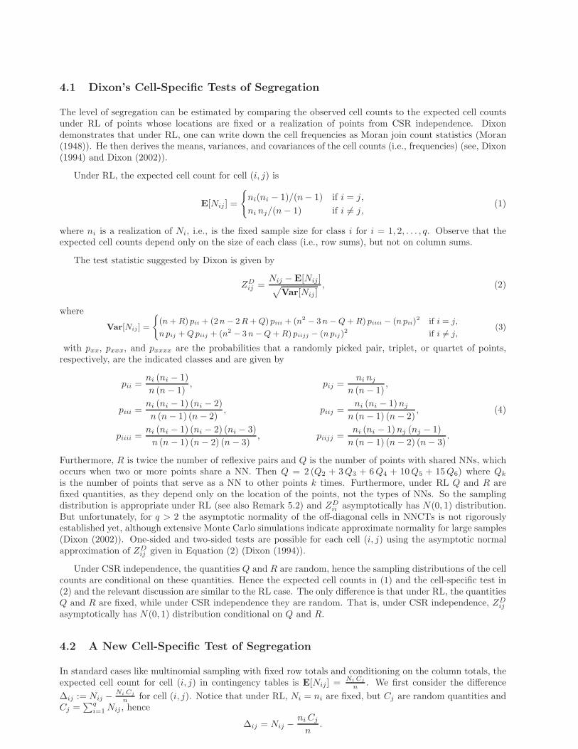
We plot the empirical power estimates for the NNCT-tests in Figures 5 and 6. The test statistics are mostly positivefor diagonal cells which implies segregation of classes and are mostly negative for off-diagonal cells which implies lack
17
Empirical Power Estimates of Cell-Specific Tests under HS
2 4 6 8 10 12
0.0
0.2
0.4
0.6
0.8
1.0
empi
rical
pow
er
cell (1,1)
2 4 6 8 10 12
0.0
0.2
0.4
0.6
0.8
1.0
empi
rical
pow
er
cell (1,2)
2 4 6 8 10 12
0.0
0.2
0.4
0.6
0.8
1.0
empi
rical
pow
er
cell (1,3)
2 4 6 8 10 12
0.0
0.2
0.4
0.6
0.8
1.0
empi
rical
pow
er
cell (2,1)
2 4 6 8 10 12
0.0
0.2
0.4
0.6
0.8
1.0
empi
rical
pow
er
cell (2,2)
2 4 6 8 10 12
0.0
0.2
0.4
0.6
0.8
1.0
empi
rical
pow
er
cell (2,3)
2 4 6 8 10 12
0.0
0.2
0.4
0.6
0.8
1.0
empi
rical
pow
er
cell (3,1)
2 4 6 8 10 12
0.0
0.2
0.4
0.6
0.8
1.0
empi
rical
pow
er
cell (3,2)
2 4 6 8 10 12
0.0
0.2
0.4
0.6
0.8
1.0
empi
rical
pow
er
cell (3,3)
Figure 5: The empirical power estimates of Dixon’s cell-specific tests (circles (◦)) and the new cell-specific tests(triangles (△)) under the segregation alternatives HS1
(black), HS2(red), and HS3
(blue) in the three-classcase. The horizontal axis labels are: 1=(10,10,10), 2=(10,10,30), 3=(10,10,50), 4=(10,30,30), 5=(10,30,50),6=(30,30,30), 7=(10,50,50), 8=(30,30,50), 9=(30,50,50), 10=(50,50,50), 11=(50,50,100), 12=(50,100,100),13=(100,100,100). Notice that they are arranged in the increasing order for the first and then the secondentries. The size values for discrete sample size combinations are joined by piecewise straight lines for bettervisualization.
18

Empirical Power Estimates of Overall Tests under HS
2 4 6 8 10 12
0.0
0.2
0.4
0.6
0.8
1.0
empi
rical
pow
er overall
Figure 6: The empirical power estimates of Dixon’s overall test (circles (◦)) and the new overall test (triangles(△)) under the segregation alternatives HS1
(black), HS2(red), and HS3
(blue) in the three-class case. Thehorizontal axis labels are as in Figure 5.
of association between classes. For both cell-specific tests for the diagonal cells (i, i) for i = 1, 2, 3, as equal samplesizes get larger, the power estimates get larger under each segregation alternative; and as the segregation gets stronger,the power estimates get larger for each cell at each sample size combination. The higher degree of segregation betweenX and Y is reflected in cells (1, 1) and (2, 2). Furthermore, since the sample sizes satisfy n1 ≤ n2 in our simulationstudy, cell (2, 2) power estimates tend to be larger. Since class Z is less segregated from the other two classes, cell(3, 3) power estimates tend to be lower than the other diagonal cell statistics. Notice also that off-diagonal cells aremore severely affected by the differences in the sample sizes.
The higher degree of segregation between classes X and Y can also be observed in cells (1, 2) and (2, 1) powerestimates, since more segregation of these classes imply higher negative values in these cells’ test statistics. The lesserdegree of segregation between classes X and Z can be observed in cells (1, 3) and (3, 1), as they yield much lowerpower estimates compared to the other cells. Although Y and Z are segregated in the same degree as X and Z, thepower estimates for cells (2, 3) and (3, 2) are larger than those for cells (1, 3) and (3, 1), since (n1 + n3) ≤ (n2 + n3) inour simulation study and larger sample sizes imply higher power under the same degree of segregation.
Furthermore, the power estimates for the new cell-specific tests tend to be higher for each cell under each segregationalternative for each sample size combination. In summary, in the three-class case, new cell-specific tests have betterperformance in terms of power.
The performance of the overall tests are similar to the performance of cell-specific tests for the diagonal cells:power estimates increase as the segregation gets stronger; power estimates increase as the sample sizes increase; andnew overall test has higher power than Dixon’s overall test.
The empirical power estimates based on the Monte Carlo critical values yield similar results, hence not presented.
Considering the empirical significance levels and power estimates, for small samples we recommend Monte Carlorandomization for these tests; for larger samples we recommend the new versions of the overall and cell-specific testsfor testing against the segregation alternatives, as they either have about the same power as or have larger power thanDixon’s tests. Furthermore, if one wants to see the level of segregation between pairs of classes, we recommend usingthe diagonal cells, (i, i) for i = 1, 2, 3 as they are more robust to the differences in class sizes (i.e., relative abundance)and more sensitive to the level of segregation.
10.2 Empirical Power Analysis under Association of Three Classes
For the association alternatives, we also consider three cases. In each case, first we generate Xiiid∼ U((0, 1) × (0, 1))
for i = 1, 2, . . . , n1. Then we generate Yj and Zℓ for j = 1, 2, . . . , n2 and ℓ = 1, 2, . . . , n3 as follows. For each j, we pick
an i randomly, then generate RYj
iid∼ U(0, ry) with ry ∈ (0, 1) and Tjiid∼ U(0, 2π) set Yj := Xi + RY
j (cos Tj , sin Tj)′.
19

Similarly, for each ℓ, we pick an i randomly, then generate RZℓ
iid∼ U(0, rz) with rz ∈ (0, 1) and Uℓiid∼ U(0, 2π) and set
Zℓ := Xi + RZℓ (cos Uℓ, sin Uℓ)
′.
In the pattern generated, appropriate choices of ry (and rz) values will imply association between classes X andY (and X and Z). The three association alternatives are
HA1: ry = 1/7, rz = 1/10, HA2
: ry = 1/10, rz = 1/20, HA3: ry = 1/13, rz = 1/30. (19)
Observe that, from HA1to HA3
(i.e., as ry and rz decrease), the association between X and Y gets stronger in thesense that Y points tend to be found more and more frequently around the X points. Likewise for X and Z points.Furthermore, by construction, classes X and Z are more associated compared to classes X and Y .
Empirical Power Estimates of Cell-Specific Tests under HA
2 4 6 8 10 12
0.0
0.2
0.4
0.6
0.8
1.0
empi
rical
pow
er
cell (1,1)
2 4 6 8 10 12
0.0
0.2
0.4
0.6
0.8
1.0
empi
rical
pow
er
cell (1,2)
2 4 6 8 10 12
0.0
0.2
0.4
0.6
0.8
1.0
empi
rical
pow
er
cell (1,3)
2 4 6 8 10 12
0.0
0.2
0.4
0.6
0.8
1.0
empi
rical
pow
er
cell (2,1)
2 4 6 8 10 12
0.0
0.2
0.4
0.6
0.8
1.0
empi
rical
pow
er
cell (2,2)
2 4 6 8 10 12
0.0
0.2
0.4
0.6
0.8
1.0
empi
rical
pow
er
cell (2,3)
2 4 6 8 10 12
0.0
0.2
0.4
0.6
0.8
1.0
empi
rical
pow
er
cell (3,1)
2 4 6 8 10 12
0.0
0.2
0.4
0.6
0.8
1.0
empi
rical
pow
er
cell (3,2)
2 4 6 8 10 12
0.0
0.2
0.4
0.6
0.8
1.0
empi
rical
pow
er
cell (3,3)
Figure 7: The empirical power estimates of Dixon’s cell-specific tests (circles (◦)) and the new cell-specifictests (triangles (△)) under the association alternatives HA1
(black), HA2(red), and HA3
(blue) in the three-class case. The horizontal axis labels are as in Figure 5.
The power estimates for the NNCT-tests are plotted in Figures 7 and 8. The test statistics tend to be negativefor the diagonal cells, which implies lack of segregation for the classes; positive for cells (1, 2), (2, 1), (1, 3), and (3, 1),which implies association between classes X and Y and association between classes X and Y ; negative for cells (2, 3)and (3, 2), which implies lack of association (and perhaps mild segregation) between classes Y and Z.
20

Empirical Power Estimates of Overall Tests under HA
2 4 6 8 10 12
0.0
0.2
0.4
0.6
0.8
1.0
empi
rical
pow
er
overall
Figure 8: The empirical power estimates of Dixon’s overall test (circles (◦)) and the new overall test (triangles(△)) under the association alternatives HA1
(black), HA2(red), and HA3
(blue) in the three-class case. Thehorizontal axis labels are as in Figure 5.
At each sample size combination, as the association gets stronger, the power estimates increase. Further, thehigher degree of association between X and Z compared to that of X and Y are reflected in higher power estimatesfor cell (1, 3) compared to cell (1, 2). For the same reason, power estimates for cell (3, 1) are higher than those for cell(2, 1).
For cells (1, 2), (2, 1), (1, 3), and (3, 1) the power estimates get larger as the equal sample sizes increase. Thenew cell-specific tests have higher power for cells (1, 2) and (1, 3) and Dixon’s cell-specific tests have higher power forcells (2, 1) and (3, 1). By construction the classes Y and Z are not associated, instead they can be viewed as mildlysegregated from each other. The test statistics for cells (2, 3) and (3, 2) are negative to indicate such segregation orlack of association between classes Y and Z. However, cell (3, 2) power estimates are much larger than cell (3, 2),which implies that class Z can be viewed as more segregated from class Y . As for the diagonal cells, the higher powerestimates for cell (1, 1) for larger samples are indicative of high degree of association of classes Z and Y with class X.Such association, by construction, is barely reflected in cells (2, 2) and (3, 3).
In summary, for cells (i, j) with i < j, the new tests have higher power, while for cells (i, j) with i > j, Dixon’stests have higher power. For the diagonal cells both versions of the cell-specific tests have about the same powerperformance. So we recommend both versions of cell-specific tests to be applied in a given situation and the resultscompared and interpreted carefully.
The power estimates of the overall tests tend to increase as the association gets stronger at each sample sizecombination; as the sample sizes tend to increase, except for the sudden decrease at (n1, n2, n3) = (10, 50, 50), inwhich case cell (1, 1) counts and column 1 sums tend to be very small. Furthermore, Dixon’s overall test has higherpower compared to the new overall test. So Dixon’s overall test is recommended for the association alternative overthe new overall test.
The empirical power estimates based on the Monte Carlo critical values yield similar results, hence not presented.
Remark 10.1. Main Result of Monte Carlo Power Analysis: Based on the recommendations made in Remark7.1, when at least one sample size is small (in the sense that some cell count is < 5), we recommend Monte Carlorandomization for the NNCT-tests. For large samples, one can use asymptotic or Monte Carlo versions of the NNCT-tests. In Sections 9.1, 9.2, 10.1, and 10.2, we observe that under the segregation alternatives, the new cell-specificand new overall tests have higher power compared to Dixon’s cell-specific and overall tests. Under the associationalternatives, we observe that for cells with the associated class is the NN class, the new cell-specific tests have higherpower, while for cells with the associated class as the base class, Dixon’s cell-specific tests have higher power, andfor diagonal cells Dixon’s and new cell-specific tests have similar power. Additionally, Dixon’s overall test has higherpower than the new overall test for association. Thus we recommend both of the new and Dixon’s NNCT-tests underthe association alternatives. �
21

11 Examples
We illustrate the tests on two ecological data sets: Pielou’s Douglas-fir/ponderosa pine data (Pielou (1961)) and a
swamp tree data (Good and Whipple (1982)).
11.1 Pielou’s Data
Pielou (1961) used a completely mapped data set that is comprised of two tree species: Douglas-fir trees(Pseudotsuga menziesii formerly P. taxifolia) and ponderosa pine (Pinus ponderosa) from a region in BritishColumbia. Her data set was also used by Dixon as an illustrative example (Dixon (1994)). The question ofinterest is the type of spatial interaction between the two tree species. The corresponding 2 × 2 NNCT andthe percentages for each cell are provided in Table 9. The cell percentages are with respect to the samplesizes of each species, for example, 86 % of Douglas-firs have NNs from Douglas firs and remaining 15 % ofDouglas-firs have NNs from ponderosa pines. The row and column percentages are marginal percentages withrespect to the total sample size. The percentage values are suggestive of segregation for both species.
The raw data are not available, hence we can not perform Monte Carlo simulation nor randomizationversions of the tests. Fortunately, Pielou (1961) provided Q = 162 and R = 134, hence we can calculate thetest statistics and use the asymptotic approximation for these tests. The overall and cell-specific test statisticsand the corresponding p-values (in parentheses) based on the asymptotic approximation, denoted by pasy,are provided in Table 10. Although the locations of the tree species are not known, they can be viewed apriori resulting from different processes rather than some process affecting a posteriori the individuals of asingle population. So the more appropriate null hypothesis is CSR independence of the trees. Hence ourinference will be a conditional one (see Remark 5.2). Observe that Dixon’s and new overall test statisticsyield significant p-values, implying some sort of deviation from CSR independence. In order to see the type ofdeviation, we apply the cell-specific tests. Both versions of the cell-specific tests for each cell are significant,implying significant deviation from CSR independence. The cell-specific test statistics are positive for thediagonal cells (1, 1) and (2, 2) (and negative for the off-diagonal cells (1, 2) and (2, 1)), implying segregationfor both species. This is in agreement with what the NNCT suggests and the findings of (Dixon (1994)).However, Dixon’s cell (1, 1) statistics are much larger than cell (2, 2) statistics, which may be interpreted asclustering of Douglas-firs is stronger than the clustering of ponderosa pines. Our simulation study indicatesthat this might be an artifact of the relative abundance of the tree species. On the other hand, new cell (1, 1)and cell (2, 2) statistics are very similar, hence the segregation of both tree species are at about the samedegree.
11.2 Swamp Tree Data
Good and Whipple (1982) considered the spatial interaction between tree species along the Savannah River,South Carolina, U.S.A. From this data, Dixon (2002) used a single 50m × 200m rectangular plot to illustratehis NNCT-tests. All live or dead trees with 4.5 cm or more dbh (diameter at breast height) were recordedtogether with their species. Hence it is an example of a realization of a marked multi-variate point pattern. Theplot contains 13 different tree species, four of which comprises over 90 % of the 734 tree stems. The remainingtree stems were categorized as “other trees”. The plot consists of 215 water tupelos (Nyssa aquatica), 205 blackgums (Nyssa sylvatica), 156 Carolina ashes (Fraxinus caroliniana), 98 bald cypresses (Taxodium distichum),and 60 stems from 8 additional species (i.e., other species). A 5×5 NNCT-analysis is conducted for this dataset. If segregation among the less frequent species is important, a more detailed 12×12 NNCT-analysis shouldbe performed. The locations of these trees in the study region are plotted in Figure 9 and the corresponding5× 5 NNCT together with percentages based on row and grand sums are provided in Table 11. For example,for black gum as the base species and Carolina ash as the NN species, the cell count is 26 which is 13 % ofthe 205 black gums (which is 28 % of all trees). Observe that the percentages and Figure 9 are suggestive ofsegregation for all tree species, especially for Carolina ashes, water tupelos, black gums, and the “other” treessince the observed percentages of species with themselves as the NN are much larger than the row percentages.
The locations of the tree species can be viewed a priori resulting from different processes, so the moreappropriate null hypothesis is the CSR independence pattern. Hence our inference will be a conditional one
22

0 50 100 150 200
010
2030
4050
Swamp Tree Data
x coordinate (m)
y co
ordi
nate
(m
)
Figure 9: The scatter plot of the locations of water tupelos (triangles △), black gum trees (pluses +), Carolinaashes (crosses ×), bald cypress trees (diamonds ⋄), and other trees (inverse triangles ▽).
(see Remark 5.2). We calculate Q = 472 and R = 454 for this data set. We present Dixon’s overall test ofsegregation and cell-specific test statistics and the associated p-values in Table 12, where pasy stands for thep-value based on the asymptotic approximation, pmc is the p-value based on 10000 Monte Carlo replicationof the CSR independence pattern in the same plot and prand is based on Monte Carlo randomization of thelabels on the given locations of the trees 10000 times. Notice that pasy, pmc, and prand are very similar foreach test. We present the new overall test of segregation and cell-specific test statistics and the associatedp-values in Table 13, where p-values are calculated as in Table 12. Again, all three p-values in Table 13 aresimilar for each test.
Dixon’s and the new overall test of segregation are both significant implying significant deviation from theCSR independence pattern for at least for one pair of the tree species. Then to determine which pairs exhibitsegregation or association, we perform the cell-specific tests. Dixon’s and the new cell-specific tests agree forall cells (i.e., pairs) in term of significance at .05 level except for (B.G.,B.C.), (BC,W.T), and (B.C.,C.A.)pairs. The statistics are all negative for the off-diagonal cells, except for (B.C.,C.A.) and (C.A., B.C.) pairs.Based on the Monte Carlo simulation analysis, the new test is more reliable to attach significance to thesesituations. The spatial interaction is significant between each pair which does not contain bald cypresses.That is, the new cell-specific test statistics are positive for the diagonal cells (i, i) for i = 1, 2, . . . , 5 and aresignificant for i = 1, 2, 3, 5 at .05 level (which also holds for Dixon’s tests); and are negative for the off-diagonalcells (i, j) with i, j ∈ {1, 2, 3, 5} and i 6= j and significant for most of them. Hence each tree species except baldcypresses exhibits significant segregation from each other. These findings are mostly in agreement with theresults of (Dixon (2002)). Hence except for bald cypresses, each tree species seem to result from a (perhaps)different first order inhomogeneous Poisson process.
Based on the NNCT-tests above, we conclude that all tree species but bald cypresses exhibit significantdeviation from the CSR independence pattern. Considering Figure 9, the corresponding NNCT in Table11, and the cell-specific test results in Tables 12 and 13, this deviation is toward the segregation of the treespecies. However, these results pertain to small scale interaction at about the average NN distances. Wemight also be interested in the causes of the segregation and the type and level of interaction between thetree species at different scales (i.e., distances between the trees). To answer such questions, we also presentthe second-order analysis of the swamp tree data. We calculate Ripley’s (univariate) L-function which is the
modified version of K function as Lii(t) =
√(Kii(t)/π
)where t is the distance from a randomly chosen
23

0 2 4 6 8 10 12
−0.
10.
00.
10.
20.
3
All Trees
t(m)
L 00(t
)−t
0 2 4 6 8 10 12
−0.
50.
00.
51.
01.
5
Water Tupelos
t(m)L 1
1(t)−
t
0 2 4 6 8 10 12
−0.
50.
00.
51.
01.
5
Black Gums
t(m)
L 22(t
)−t
0 2 4 6 8 10 12
−1
01
23
45
Caroline Ashes
t(m)
L 33(t
)−t
0 2 4 6 8 10 12
−1
01
2Bald Cypresses
t(m)
L 44(t
)−t
0 2 4 6 8 10 12
−2
02
46
Other Trees
t(m)
L 55(t
)−t
Figure 10: Second-order analysis of swamp tree data. Functions plotted are Ripley’s univariate L-functionsLii(t) − t for i = 0, 1, . . . , 5, where i = 0 stands for all data combined, i = 1 for water tupelos, i = 2 forblack gums, i = 3 for Carolina ashes, i = 4 for bald cypresses, and i = 5 for other trees. Wide dashed linesaround 0 (which is the theoretical value) are the upper and lower (pointwise) 95 % confidence bounds for theL-functions based on Monte Carlo simulation under the CSR independence pattern.
event (i.e., location of a tree), Kii(t) is an estimator of
K(t) = λ−1E[# of extra events within distance t of a randomly chosen event] (20)
with λ being the density (number per unit area) of events and is calculated as
Kii(t) = λ−1∑
i
∑
j 6=i
w(li, lj)I(dij < t)/N (21)
where λ = N/A is an estimate of density (N is the observed number of points and A is the area of the studyregion), dij is the distance between points i and j, I(·) is the indicator function, w(li, lj) is the proportionof the circumference of the circle centered at li with radius dij that falls in the study area, which correctsfor the boundary effects. Under CSR independence, L(t) − t = 0 holds. If the univariate pattern exhibitsaggregation, then L(t)− t tends to be positive, if it exhibits regularity then L(t)− t tends to be negative. The
estimator K(t) is approximately unbiased for K(t) at each fixed t. Bias depends on the geometry of the studyarea and increases with t. For a rectangular region it is recommended to use t values up to 1/4 of the smallerside length of the rectangle. See (Diggle (2003)) for more detail. So we take the values t ∈ [0, 12.5] in ouranalysis, since the smaller side of the rectangular region of swamp tree data is 50 m. In Figure 10, we presentthe plots of Lii(t)− t functions for each species as well as the plot of all trees combined. We also present theupper and lower (pointwise) 95 % confidence bounds for each Lii(t) − t. Observe that for all trees combinedthere is significant aggregation of trees (the L00(t)− t curve is above the upper confidence bound) at all scales(i.e., distances). Water tupelos exhibit significant aggregation for the range of the plotted distances; blackgums exhibit significant aggregation for distances t > 1 m; Carolina ashes exhibit significant aggregation forthe range of plotted distances; bald cypresses exhibit no deviation from CSR independence for t . 5 m, thenthey exhibit significant spatial aggregation for t > 4 m; other trees exhibit significant aggregation for therange of plotted distances. Hence, segregation of the species might be due to different levels and types ofaggregation of the species in the study region.
24

0 2 4 6 8 10 12
0.7
0.8
0.9
1.0
1.1
1.2
1.3
All Trees
t(m)
g(t)
0 2 4 6 8 10 12
0.5
1.0
1.5
2.0
2.5
3.0
3.5
Water Tupelos
t(m)g(
t)
0 2 4 6 8 10 12
0.5
1.0
1.5
2.0
Black Gums
t(m)
g(t)
0 2 4 6 8 10 12
12
34
Carolina Ashes
t(m)
g(t)
0 2 4 6 8 10 12
0.5
1.0
1.5
2.0
2.5
Bald Cypresses
t(m)
g(t)
0 2 4 6 8 10 12
02
46
8
Other Trees
t(m)
g(t)
Figure 11: Pair correlation functions for all trees combined and for each species in the swamp tree data. Widedashed lines around 1 (which is the theoretical value) are the upper and lower (pointwise) 95 % confidencebounds for the L-functions based on Monte Carlo simulation under the CSR independence pattern.
We also calculate Ripley’s bivariate L-function as Lij(t) =
√(Kij(t)/π
)where Kij(t) is an estimator of
Kij(t) = λ−1j E[# of extra type j events within distance t of a randomly chosen type i event]
with λj being the density of type j events. Then Kij(t) is calculated as
Kij(t) =(λiλjA
)−1 ∑
i
∑
j
w(ik, jl)I(dik ,jl< t), (22)
where dik,jlis the distance between kth type i and lth type j points, w(ik, jl) is the proportion of the
circumference of the circle centered at kth type i point with radius dik,jlthat falls in the study area, which is
used for edge correction. Notice that by construction, Lij(t) is symmetric in i and j, that is, Lij(t) = Lji(t) forall i, j. Under CSR independence, Lij(t)− t = 0 holds. If the bivariate pattern is segregation, then Lij(t)− ttends to be negative, if it is association then Lij(t) − t tends to be positive. See (Diggle (2003)) for more
detail. In Figure 12, we present the bivariate plots of Lij(t) − t functions together with the upper and lower
(pointwise) 95 % confidence bounds for each pair of species (due to the symmetry of Lij(t) there are only 10different pairs). Observe that for distances up to t ≈ 10 m, water tupelos and black gums exhibit significant
segregation (L12(t) − t is below the lower confidence bound) and for the rest of the plotted distances theirinteraction is not significantly different from the CSR independence pattern; water tupelos and Carolina ashesare significantly segregated up to about t ≈ 10 m; water tupelos and bald cypresses do not have significantdeviation from the CSR independence pattern for distances up to 4 m, for larger distances they exhibitsignificant segregation; water tupelos and the other trees do not deviate from CSR independence for therange of the plotted distances. Black gums and Carolina ashes are significantly segregated for t > 2 m; blackgums and bald cypresses are significantly segregated for t > 2 m; black gum and other trees are significantlysegregated for all the distances plotted. Carolina ashes and bald cypresses are significantly associated fordistances larger than 3 m; and Carolina ashes and the other trees exhibit significant segregation for 3 < t < 7
25

m and for t > 11 m they exhibit significant association. On the other hand, bald cypresses and other treesare significantly associated for distance larger than 4 m.
But Ripley’s K-function is cumulative, so interpreting the spatial interaction at larger distances is prob-lematic (Wiegand et al. (2007)). The (accumulative) pair correlation function g(t) is better for this purpose(Stoyan and Stoyan (1994)). The pair correlation function of a (univariate) stationary point process is definedas
g(t) =K ′(t)
2 π t
where K ′(t) is the derivative of K(t). For a univariate stationary Poisson process, g(t) = 1; values of g(t) < 1suggest inhibition (or regularity) between points; and values of g(t) > 1 suggest clustering (or aggregation).The pair correlation functions for all trees and each species for the swamp tree data are plotted in Figure11. Observe that all trees are aggregated around distance values of 0-1,3,4,5,7,9-10 m; water tupelos areaggregated for distance values of 0-4 and 5-7 m; black gums are aggregated for distance values of 1-6 and 8-11m; Carolina ashes are aggregated for all the range of the plotted distances; bald cypresses are aggregated fordistance values of 2-8 and around 11 m; and other trees are aggregated for all distance values except 3-5 m.Comparing Figures 10 and 11, we see that Ripley’s L and pair correlation functions detect the same patternsbut with different distance values. That is, Ripley’s L implies that the particular pattern is significant for awider range of distance values compared to g(t), since Ripley’s L is cumulative, so the values of L at smallscales confound the values of L at larger scales (Loosmore and Ford (2006)). Hence the results based on paircorrelation function g(t) are more reliable.
The same definition of the pair correlation function can be applied to Ripley’s bivariate K or L-functionsas well. The benchmark value of Kij(t) = π t2 corresponds to g(t) = 1; g(t) < 1 suggests segregation of theclasses; and g(t) > 1 suggests association of the classes. The bivariate pair correlation functions for the speciesin swamp tree data are plotted in Figure 13. Observe that water tupelos and black gums are segregated fordistance values of 0-1 m; water tupelos and Carolina ashes are segregated for values of 0-1 and 2.5 m and areassociated for values about 6 m; water tupelos and bald cypresses are segregated for 0-1, 5.5, 9.5, and 11 mand are associated for 6.5 m; water tupelos and other trees are segregated for 0-0.5 and 7 m and are associatedfor 8 m; black gums and Carolina ashes are segregated for 2-2.5, 3.5-4.5, 6-8.5, and 9.5-12 m; black gums andbald cypresses are segregated for 3.5, 5.5-6.5,7, and 9.5 m; black gums and other trees are segregated for 5and 6-7.5 m; Carolina ashes and bald cypresses are associated for 1.5-3, 5.5., and 7 m; Carolina ashes andother trees are associated for 5 and 9-10 m; and bald cypresses and other trees are segregated for 4 m andare associated for 3-4 and 6.5-7.5 m.
However the pair correlation function estimates might have critical behavior for small t if g(t) > 0 sincethe estimator variance and hence the bias are considerably large. This problem gets worse especially in clusterprocesses (Stoyan and Stoyan (1996)). See for example Figures 11 and 13 where the confidence bands forsmaller t values are much wider compared to those for larger t values. So pair correlation function analysis ismore reliable for larger distances and it is safer to use g(t) for distances larger than the average NN distancein the data set. Comparing Figure 10 with Figure 11 and Figure 12 with Figure 13 we see that Ripley’s Land pair correlation functions usually detect the same large-scale pattern but at different ranges of distancevalues. Ripley’s L suggests that the particular pattern is significant for a wider range of distance valuescompared to g(t), since values of L at small scales confound the values of L at larger scales where g(t) is morereliable to use (Loosmore and Ford (2006)).
While second order analysis (using Ripley’s K and L-functions or pair correlation function) provides in-formation on the univariate and bivariate patterns at all scales (i.e., for all distances), NNCT-tests summarizethe spatial interaction for the smaller scales (for distances about the average NN distance in the data set). Inparticular, for the swamp tree data average NN distance (± standard deviation) is about 1.8 (± 1.04) metersand notice that Ripley’s L-function and NNCT-tests yield similar results for distances about 2 meters.
12 Discussion and Conclusions
In this article we introduce new overall and cell-specific tests of segregation based on nearest neighbor con-tingency tables (NNCTs). Such tests are referred to as NNCT-tests. We also consider Dixon’s NNCT-tests,discuss the differences in these (new and Dixon’s) NNCT-tests, present the asymptotic properties of them,
26

compare the tests using extensive Monte Carlo simulations under RL and CSR independence and under var-ious segregation and association alternatives for two and three classes. We also illustrate the tests on twoexamples and compare them with Ripley’s L-function (Ripley (2004)).
NNCT-tests (i.e., overall and cell-specific tests of segregation) are used in testing randomness in the nearestneighbor (NN) structure between two or more classes. The overall test is used for testing any deviation fromrandomness in all the NNCT cells combined; cell-specific test for cell (i, j) is used for testing any deviationfrom randomness in cell (i, j), i.e., NN structure in which base class is i and NN class is j. This statistictests the segregation or lack of it if i = j; the association or lack of it between classes i and j if i 6= j. Therandomness in the NN structure is implied by the RL or CSR independence patterns. We demonstrate thatunder the CSR independence pattern, NNCT-tests are conditional on Q and R, while under the RL pattern,these tests are unconditional. In the two-class case, cell-specific tests are essentially different only for twocells, since cell (1, 1) and (1, 2) yield the same test statistic in absolute value for Dixon’s cell-specific test,likewise for cells (2, 1) and (2, 2). Similarly, cell (1, 1) and (2, 1) yield the same test statistic in absolute valuefor the new cell-specific test, likewise for cells (1, 2) and (2, 2).
Based on our Monte Carlo simulations, we conclude that the asymptotic approximation for the cell-specific-tests is appropriate only when the corresponding cell count in the NNCT is larger than 10; and for the overalltest when all cell counts are larger than 4. When at least one cell count is less than 5, we recommend theMonte Carlo randomization version of the overall tests; and when a cell count is less than 10, we recommendthe Monte Carlo randomization of the cell-specific tests. When each cell count is larger than 5, the newversions of the segregation tests have empirical significance levels closer to the nominal level. Type I errorrates (empirical significance levels) of the new cell-specific tests are more robust to the differences in samplesizes (i.e., differences in relative abundance). When some cell count(s) are less than 5 for overall test andless than 10 for the cell-specific tests, we compare the power of the tests using Monte Carlo critical values.For large samples, the power comparisons can be made using both the asymptotic or Monte Carlo criticalvalues. For the segregation alternatives, we conclude that the new cell-specific and overall tests have higherpower estimates compared to those of Dixon’s tests. For the association alternatives, we observe that thebest performer NNCT-test depends on the cell and level of association. When testing against association, thenew cell-specific tests have higher power estimates for the upper triangular cells in the NNCT and Dixon’scell-specific tests have higher power estimates for the lower triangular cells in the NNCT. We recommendthe new cell-specific and overall tests for the segregation alternatives. For the association alternatives, werecommend both versions of the overall and cell-specific tests.
The CSR independence pattern assumes that the study region is unbounded for the analyzed pattern,which is not the case in practice. Edge effects are a constant problem in the analysis of empirical (i.e., bounded)data sets and much effort has gone into the development of edge corrections methods (Yamada and Rogersen(2003)). So the edge (or boundary) effects might confound the test results if the null pattern is the CSRindependence. Two correction methods for the edge effects on NNCT-tests, namely buffer zone correctionand toroidal correction, are investigated in (Ceyhan (2007)) where it is shown that the empirical sizes ofthe NNCT-tests are mildly affected by the toroidal edge correction. However, the (outer) buffer zone edgecorrection method seems to have slightly stronger influence on the tests compared to toroidal correction. Butfor these tests, buffer zone correction does not change the sizes significantly for most sample size combinations.This is in agreement with the findings of Barot et al. (1999) who say NN methods only require a small bufferarea around the study region. A large buffer area does not help much since one only needs to be able to seefar enough away from an event to find its NN. Once the buffer area extends past the likely NN distances (i.e.,about the average NN distances), it is not adding much helpful information for NNCTs. Hence we recommendinner or outer buffer zone correction for NNCT-tests with the width of the buffer area being about the averageNN distance. We do not recommend larger buffer areas, since they are wasteful with little additional gain.On the other hand, we recommend the use of toroidal edge correction with points within the average NNdistance in the additional copies around the study region. For larger distances, the gain might not be worththe effort.
NNCT-tests summarize the pattern in the data set for small scales, more specifically, they provide infor-mation on the pattern around the average NN distance between all points. On the other hand, pair correlationfunction g(t) and Ripley’s classical K or L-functions and other variants provide information on the pattern atvarious scales. However, the classical L-function is not appropriate for the null pattern of RL when locationsof the points have spatial inhomogeneity. For such cases, Diggle’s D-function (Diggle (2003) p. 131) is more
27

appropriate in testing the bivariate spatial clustering at various scales.
Ripley’s classical K(t) or L(t) functions can be used when the null pattern can be assumed to be CSRindependence, that is when the null pattern assumes first-order homogeneity for each class. When the nullpattern is the RL of points from an inhomogeneous Poisson process they are not appropriate (Kulldorff (2006));Cuzick-Edward’s k-NN tests are designed for testing bivariate spatial interaction and mostly used for spatialclustering of cases in epidemiology; Diggle’s D-function is a modified version of Ripley’s K-function (Diggle(2003)) and adjusts for any inhomogeneity in the locations of, e.g., cases and controls. Furthermore, there arevariants of K(t) that explicitly correct for inhomogeneity (see Baddeley et al. (2000)). Ripley’s K−, Diggle’sD-functions and pair correlation functions are designed to analyze univariate or bivariate spatial interactionat various scales (i.e., inter-point distances). Our example illustrates that for distances around the averageNN distance, NNCT-tests and Ripley’s bivariate L-function yield similar results.
The NNCT-tests and Ripley’s L-function provide similar information in the two-class case at small scales.For q-class case with q > 2 classes, overall tests provide information on the (small-scale) while the Ripley’sL-function requires performing all bivariate spatial interaction analysis. The cell-specific tests can serve aspairwise post hoc analysis only when the overall test is significant. Furthermore, the cell-specific tests aretesting the spatial clustering of one class or bivariate interaction between two classes as part of the multivariateinteraction between all the classes. On the other hand, Ripley’s univariate K- or L-functions are restricted toone class and bivariate K- or L-functions are restricted to two classes they pertain to, ignoring the potentiallyimportant multivariate interaction between all classes in the study area. However, there are forms of the J-function which is derived from the well-known G and F functions (van Lieshout and Baddeley (1999)) anddeal with this multi-type setting (i.e., consider the pattern of type i in the context of the pattern of all othertypes). van Lieshout and Baddeley (1999) define two basic types of J-functions. First is a type-i-to-type-jfunction which considers the points of type i in the context of the points of type j. The second one is thetype-i-to-any-type function which considers the points of type i in the context of points of all types includingtype i. Other forms can be derived from them by re-defining the types. For example, if we want to considerthe points of type i in the context of points of all other types, then we collapse all the other types j (i.e., allj which are not equal to i) into a single type i′ and then use the type-i-to-type-i′ function. Several authorshave written about the bivariate K-function, which is of the type-i-to-type-j form (Diggle and Chetwynd(1991), Haase (1995), and Diggle (2003)). Type-i-to-type-j K-function can easily be modified to type-i-to-any-type K-function. Thus essentially there is only one family of multi-type K-functions in literature. Buttype-i-to-type-j K-function is comparable with a NNCT analysis based on a 2 × 2 NNCT restricted to theclasses i and j. Similarly, type-i-to-type-i′ K-function is comparable with the NNCT analysis based on a2 × 2 NNCT with classes i and the rest of the classes labeled as i′. Since pairwise analysis of q classeswith 2× 2 NNCTs might yield conflicting results compared to q × q NNCT analysis (Dixon (2002)), Ripley’sL-function and NNCT-tests might also yield conflicting results at small distances. Hence Ripley’s L-functionand NNCT-tests may provide similar but not identical information about the spatial pattern and the lattermight provide small-scale interaction that is not detected by the former. Since the pair correlation functionsare derivatives of Ripley’s K-function, most of the above discussion holds for them also, except g(t) is reliableonly for large scale interaction analysis. Hence NNCT-tests and pair correlation function are not comparablebut provide complimentary information about the pattern in question.
Cell-specific tests for diagonal cells in a NNCT and Ripley’s univariate K- or L-functions (and hence paircorrelation functions) are symmetric, as they measure the spatial clustering of one class only. On the otherhand, Ripley’s bivariate K- or L-functions and pair correlation functions are symmetric in the two classesthey pertain to. But cell-specific tests for two classes (i.e., off-diagonal cells in the NNCT) are not symmetric.Hence, at small scales, the cell-specific test for an off-diagonal cell, provides the type and different levels ofspatial interaction for the corresponding two classes, while Ripley’s L-function and pair correlation functionprovide only the type of spatial interaction, but can not distinguish the class-specific level of interaction foreach of the two classes in question.
For a data set for which CSR independence is the reasonable null pattern, we recommend the overallsegregation test if the question of interest is the spatial interaction at small scales (i.e., about the mean NNdistance). If it yields a significant result, then to determine which pairs of classes have significant spatialinteraction, the cell-specific tests can be performed. One can also perform Ripley’s K or L-function andonly consider distances up to around the average NN distance and compare the results with those of NNCTanalysis. If the spatial interaction at higher scales is of interest, pair correlation function is recommended
28

(Loosmore and Ford (2006)), due to the cumulative nature of Ripley’s K- or L-functions for larger distances.On the other hand, if the RL pattern is the reasonable null pattern for the data, we recommend the NNCT-tests if the small-scale interaction is of interest and Diggle’s D-function if the spatial interaction at higherscales is also of interest.
Acknowledgments
I would like to thank an anonymous associate editor and two referees, whose constructive comments andsuggestions greatly improved the presentation and flow of the paper. Most of the Monte Carlo simulationspresented in this article were executed on the Hattusas cluster of Koc University High Performance ComputingLaboratory.
References
Armstrong, J. E. and Irvine, A. K. (1989). Flowering, sex ratios, pollen-ovule ratios, fruit set, and reproduc-tive effort of a dioecious tree, Myristica Insipida (Myristicacea), in two different rain forest communities.American Journal of Botany, 76:75–85.
Baddeley, A., Møller, J., and Waagepetersen, R. (2000). Non- and semi-parametric estimation of interactionin inhomogeneous point patterns. Statistica Neerlandica, 54(3):329–350.
Baddeley, A. and Turner, R. (2005). spatstat: An R package for analyzing spatial point patterns. Journal ofStatistical Software, 12(6):1–42.
Barot, S., Gignoux, J., and Menaut, J. C. (1999). Demography of a savanna palm tree: predictions fromcomprehensive spatial pattern analyses. Ecology, 80:1987–2005.
Ceyhan, E. (2007). Edge correction for cell- and class-specific tests of segregation based on nearest neigh-bor contingency tables. In Proceedings of the International Conference on Environment: Survival andSustainability, Near East University.
Coomes, D. A., Rees, M., and Turnbull, L. (1999). Identifying aggregation and association in fully mappedspatial data. Ecology, 80(2):554–565.
Cressie, N. A. C. (1993). Statistics for Spatial Data. Wiley, New York.
Cuzick, J. and Edwards, R. (1990). Spatial clustering for inhomogeneous populations (with discussion).Journal of the Royal Statistical Society, Series B, 52:73–104.
Diggle, P. J. (2003). Statistical Analysis of Spatial Point Patterns. Hodder Arnold Publishers, London.
Diggle, P. J. and Chetwynd, A. G. (1991). Second-order analysis of spatial clustering for inhomogeneouspopulations. Biometrics, 47:1155–1163.
Dixon, P. M. (1994). Testing spatial segregation using a nearest-neighbor contingency table. Ecology,75(7):1940–1948.
Dixon, P. M. (2002). Nearest-neighbor contingency table analysis of spatial segregation for several species.Ecoscience, 9(2):142–151.
Good, B. J. and Whipple, S. A. (1982). Tree spatial patterns: South Carolina bottomland and swamp forests.Bulletin of the Torrey Botanical Club, 109:529–536.
Goreaud, F. and Pelissier, R. (2003). Avoiding misinterpretation of biotic interactions with the intertypeK12-function: population independence vs. random labelling hypotheses. Journal of Vegetation Science,14(5):681–692.
Haase, P. (1995). Spatial pattern analysis in ecology based on Ripley’s K-function: Introduction and methodsof edge correction. The Journal of Vegetation Science, 6:575–582.
29

Hamill, D. M. and Wright, S. J. (1986). Testing the dispersion of juveniles relative to adults: A new analyticalmethod. Ecology, 67(2):952–957.
Herler, J. and Patzner, R. A. (2005). Spatial segregation of two common Gobius species (Teleostei: Gobiidae)in the Northern Adriatic Sea. Marine Ecology, 26(2):121–129.
Herrera, C. M. (1988). Plant size, spacing patterns, and host-plant selection in Osyris quadripartita, ahemiparasitic dioecious shrub. Journal of Ecology, 76:995–1006.
Kulldorff, M. (2006). Tests for spatial randomness adjusted for an inhomogeneity: A general framework.Journal of the American Statistical Association, 101(475):1289–1305.
Lahiri, S. N. (1996). On consistency of estimators based on spatial data under infill asymptotics. Sankhya:The Indian Journal of Statistics, Series A, 58(3):403–417.
Loosmore, N. and Ford, E. (2006). Statistical inference using the g or k point pattern spatial statistics.Ecology, 87:1925–1931.
Mat’ern, B. (1986). Spatial variation. In Lecture Notes in Statistics, edited by D. Brillinger et al., volume 36.Springer-Verlag, Berlin.
Meagher, T. R. and Burdick, D. S. (1980). The use of nearest neighbor frequency analysis in studies ofassociation. Ecology, 61(5):1253–1255.
Moran, P. A. P. (1948). The interpretation of statistical maps. Journal of the Royal Statistical Society, SeriesB, 10:243–251.
Nanami, S. H., Kawaguchi, H., and Yamakura, T. (1999). Dioecy-induced spatial patterns of two codominanttree species, Podocarpus nagi and Neolitsea aciculata. Journal of Ecology, 87(4):678–687.
Pielou, E. C. (1961). Segregation and symmetry in two-species populations as studied by nearest-neighborrelationships. Journal of Ecology, 49(2):255–269.
Ripley, B. D. (2004). Spatial Statistics. Wiley-Interscience, New York.
Searle, S. R. (2006). Matrix Algebra Useful for Statistics. Wiley-Intersciences.
Stoyan, D. and Stoyan, H. (1994). Fractals, random shapes and point fields: methods of geometrical statistics.John Wiley and Sons, New York.
Stoyan, D. and Stoyan, H. (1996). Estimating pair correlation functions of planar cluster processes. Biomet-rical Journal, 38(3):259–271.
van Lieshout, M. N. M. and Baddeley, A. J. (1999). Indices of dependence between types in multivariatepoint patterns. Scandinavian Journal of Statistics, 26:511–532.
Waagepetersen, R. P. (2007). An estimating function approach to inference for inhomogeneous Neyman-Scottprocesses. Biometrics, 63(1):252–258.
Waller, L. A. and Gotway, C. A. (2004). Applied Spatial Statistics for Public Health Data. Wiley-Interscience,NJ.
Whipple, S. A. (1980). Population dispersion patterns of trees in a Southern Louisiana hardwood forest.Bulletin of the Torrey Botanical Club, 107:71–76.
Wiegand, T., Gunatilleke, S., and Gunatilleke, N. (2007). Species associations in a heterogeneous Sri Lankandipterocarp forest. The American Naturalist, 170(4):77–95.
Yamada, I. and Rogersen, P. A. (2003). An empirical comparison of edge effect correction methods appliedto K-function analysis. Geographical Analysis, 35(2):97–109.
30

Empirical significance levels for the RL pattern
cell C
(n1, n2, n3) (1, 1) (1, 2) (1, 3) (2, 1) (2, 2) (2, 3) (3, 1) (3, 2) (3, 3)
RL Case (1)
(10,10,10) .0239c .0343c .0365c .0320c .0234c .0342c .0292c .0330c .0244c .0377c
.0469 .0422c .0418c .0411c .0471 .0440c .0385c .0452c .0452c .0422c
(10,10,30) .0498 .0361c .0273c .0399c .0488 .0287c .0430c .0517 .0432c .0455c
.0421c .0429c .0447c .0459c .0425c .0451c .0486 .0485 .0515 .0480
(10,10,50) .0676ℓ .0415c .0423c .0418c .0630ℓ .0394c .0390c .0386c .0416c .0477.0475 .0404c .0487 .0382c .0408c .0415c .0453c .0434c .0462c .0511
(10,30,30) .0737ℓ .0510 .0505 .0533 .0458c .0433c .0533 .0449c .0435c .0477.0483 .0450c .0415c .0478 .0505 .0479 .0462c .0506 .0495 .0495
(10,30,50) .0389c .0409c .0612ℓ .0660ℓ .0418c .0625ℓ .0531 .0545ℓ .0590ℓ .0518
.0444c .0535 .0539ℓ .0521 .0471 .0555ℓ .0547ℓ .0533 .0537ℓ .0547ℓ
(30,30,30) .0562ℓ .0318c .0317c .0371c .0580ℓ .0328c .0323c .0309c .0602ℓ .0471.0517 .0520 .0544ℓ .0553ℓ .0481 .0537ℓ .0539ℓ .0516 .0486 .0496
(10,50,50) .0758ℓ .0561ℓ .0498 .0303c .0620ℓ .0355c .0301c .0346c .0617ℓ .0533.0505 .0533 .0463c .0533 .0467 .0487 .0513 .0479 .0491 .0526
(30,30,50) .0493 .0400c .0505 .0407c .0479 .0550ℓ .0586ℓ .0622ℓ .0398c .0489
.0489 .0532 .0554ℓ .0494 .0463c .0559ℓ .0529 .0541ℓ .0526 .0516
(30,50,50) .0396c .0609ℓ .0649ℓ .0379c .0481 .0443c .0406c .0454c .0518 .0473.0475 .0515 .0503 .0491 .0483 .0487 .0545ℓ .0511 .0519 .0483
(50,50,50) .0483 .0453c .0454c .0468 .0521 .0468 .0436c .0510 .0500 .0469.0474 .0489 .0471 .0476 .0487 .0511 .0440c .0493 .0445c .0466
(50,50,100) .0478 .0479 .0388c .0459c .0495 .0405c .0464 .0460c .0509 .0450c
.0490 .0514 .0471 .0489 .0511 .0502 .0517 .0518 .0419c .0461c
(50,100,100) .0520 .0603ℓ .0601ℓ .0490 .0557ℓ .0504 .0467 .0501 .0491 .0476.0481 .0483 .0501 .0514 .0505 .0466 .0532 .0465 .0467 .0488
(100,100,100) .0499 .0559ℓ .0539ℓ .0563ℓ .0470 .0551ℓ .0513 .0539ℓ .0501 .0510.0484 .0515 .0495 .0537ℓ .0498 .0534 .0494 .0521 .0496 .0519
RL Case (2)
(10,10,10) .0227c .0302c .0312c .0349c .0220c .0327c .0339c .0329c .0217c .0372c
.0466 .0391c .0408c .0415c .0469 .0437c .0426c .0417c .0471 .0431c
(10,10,30) .0488 .0338c .0217c .0304c .0475 .0249c .0461c .0474 .0426c .0470.0397c .0459c .0472 .0441c .0408c .0500 .0482 .0499 .0466 .0447c
(10,10,50) .0657ℓ .0429c .0469 .0414c .0631ℓ .0412c .0443c .0459c .0501 .0501.0448c .0404c .0468 .0389c .0445c .0446c .0457c .0408c .0464 .0529
(10,30,30) .0677ℓ .0487 .0492 .0472 .0429c .0420c .0505 .0399c .0377c .0420c
.0483 .0399c .0442c .0429c .0519 .0492 .0468 .0525 .0484 .0449c
(10,30,50) .0414c .0387c .0551ℓ .0619ℓ .0599ℓ .0541ℓ .0378c .0392c .0479 .0529
.0422c .0479 .0537ℓ .0508 .0499 .0454c .0566ℓ .0461c .0505 .0528
(10,50,50) .0752ℓ .0518 .0512 .0334c .0674ℓ .0395c .0341c .0393c .0642ℓ .0507.0530 .0475 .0472 .0500 .0526 .0522 .0501 .0513 .0526 .0530
(30,30,30) .0607ℓ .0440c .0500 .0473 .0571ℓ .0468 .0496 .0462c .0622ℓ .0472.0512 .0468 .0463c .0456c .0430c .0472 .0494 .0509 .0509 .0495
(30,30,50) .0445c .0538ℓ .0459c .0598ℓ .0485 .0457c .0466 .0455c .0678ℓ .0436c
.0462c .0458c .0500 .0488 .0463c .0490 .0501 .0469 .0545ℓ .0451c
(30,50,50) .0360c .0623ℓ .0620ℓ .0371c .0472c .0437c .0379c .0441c .0504 .0475.0480 .0520 .0493 .0495 .0477 .0524 .0505 .0523 .0514 .0491
(50,50,50) .0534 .0515 .0508 .0462c .0531 .0479 .0496 .0501 .0510 .0513
.0512 .0561ℓ .0521 .0499 .0534 .0499 .0542ℓ .0540 .0512 .0462c
(50,50,100) .0462c .0480 .0429c .0497 .0464 .0414c .0458c .0473 .0512 .0497.0468 .0480 .0528 .0477 .0485 .0512 .0533 .0524 .0536 .0497
(50,100,100) .0510 .0638ℓ .0631 .0483 .0544ℓ .0539ℓ .0471 .0531 .0480 .0516.0489 .0525 .0519 .0532 .0478 .0481 .0518 .0483 .0474 .0511
(100,100,100) .0477 .0549ℓ .0525 .0499 .0473 .0571ℓ .0525 .0520 .0449c .0457c
.0491 .0518 .0494 .0487 .0479 .0541ℓ .0489 .0534 .0478 .0469
Table 5: The empirical significance levels in the three-class case under Ho : RL for RL Cases (1) and (2)with Nmc = 10000, n1, n2, n3 in {10, 30, 50, 100} at the nominal level of α = .05. (c: the empirical size issignificantly smaller than .05; i.e., the test is conservative. ℓ: the empirical size is significantly larger than.05; i.e., the test is liberal. cell = cell-specific test, C = overall test.)
31

Rejection Rates of the NNCT-Tests Under Various PCP and Inhomogeneous PatternsPCP1(np, n1, n2, σ, (0, 1) × (0, 1)) with np = 5, nc = n1/np for sample X and nc = n2/np for sample Y (same parent set for X and Y )
case 1: σ = .025 case 2: σ = .05 case 3: σ = .10sizes Dixon’s New Overall Dixon’s New Overall Dixon’s New Overall
(n1, n2) αD1,1 αD
2,2 αN1,1 αN
2,2 αD αN αD1,1 αD
2,2 αN1,1 αN
2,2 αD αN αD1,1 αD
2,2 αN1,1 αN
2,2 αD αN
(30, 30) .0814 .0716 .0726 .0719 .0709 .0735 .0779 .0701 .0707 .0717 .0675 .0727 .0719 .0656 .0630 .0619 .0611 .0631(30, 50) .0702 .0728 .0620 .0615 .0571 .0637 .0676 .0684 .0598 .0600 .0582 .0613 .0627 .0634 .0533 .0537 .0538 .0543(50, 50) .0624 .0614 .0693 .0694 .0615 .0691 .0605 .0602 .0677 .0677 .0608 .0674 .0556 .0541 .0598 .0599 .0543 .0600
(different parent sets for X and Y )(30, 30) .9993 1.000 1.000 1.000 1.000 1.000 .9880 .9882 .9959 .9958 .9922 .9957 .7641 .7622 .8527 .8522 .7806 .8522(30, 50) 1.000 .9997 1.000 1.000 1.000 1.000 .9967 .9950 .9985 .9985 .9964 .9985 .8702 .8271 .9058 .9064 .8555 .9075(50, 50) .9999 .9999 1.000 1.000 1.000 1.000 .9987 .9988 .9996 .9996 .9993 .9996 .8985 .8984 .9525 .9531 .9232 .9532
PCP2(np, n1, n2, σ, (0, 1) × (0, 1)) with np = 5, nc = n1/np for sample X and nc = n2/np for sample Y (same parent set for X and Y )(30, 30) .0509 .0498 .0465 .0475 .0472 .0470 .0523 .0509 .0459 .0470 .0475 .0469 .0512 .0485 .0428 .0438 .0448 .0440(30, 50) .0587 .0545 .0483 .0492 .0443 .0499 .0595 .0522 .0492 .0494 .0453 .0509 .0609 .0573 .0502 .0496 .0460 .0510(50, 50) .0479 .0499 .0534 .0536 .0483 .0537 .0482 .0487 .0526 .0527 .0474 .0530 .0476 .0466 .0516 .0525 .0487 .0529
(different parent sets for X and Y )(30, 30) .9993 .9998 .9999 1.000 .9998 1.000 .9884 .9878 .9953 .9953 .9910 .9953 .7779 .7812 .8624 .8633 .8007 .8627(30, 50) 1.000 .9999 1.000 1.000 .9999 1.000 .9976 .9945 .9991 .9991 .9977 .9991 .8854 .8445 .9169 .9177 .8677 .9187(50, 50) 1.000 1.000 1.000 1.000 1.000 1.000 .9987 .9991 .9997 .9997 .9995 .9997 .9182 .9112 .9607 .9600 .9354 .9602
MCP (κ, r, µ, (0, 1) × (0, 1)) with κ = 5 for both X and Y samples (same parent set for X and Y )case 1: r = .05 case 2: r = .10 case 3: r = .20
(50, 50) .0494 .0487 .0478 .0483 .0495 .0487 .0530 .0540 .0582 .0580 .0504 .0585 .0514 .0487 .0527 .0519 .0476 .0524(50, 100) .0495 .0463 .0466 .0471 .0418 .0473 .0452 .0496 .0481 .0485 .0457 .0487 .0502 .0516 .0489 .0489 .0459 .0497(100, 100) .0458 .0508 .0498 .0499 .0471 .0501 .0527 .0495 .0536 .0534 .0498 .0536 .0507 .0496 .0500 .0501 .0493 .0504
(different parent sets for X and Y )(50, 50) .9983 .9985 .9997 .9997 .9996 .9997 .9887 .9899 .9954 .9954 .9938 .9954 .8019 .8026 .8873 .8874 .8341 .8881(50, 100) .9992 .9981 .9994 .9994 .9993 .9994 .9963 .9927 .9979 .9979 .9973 .9979 .9087 .8674 .8674 .9438 .9149 .9443(100, 100) .9992 .9994 .9998 .9998 .9998 .9998 .9988 .9987 .9998 .9998 .9997 .9998 .9581 .9579 .9804 .9805 .9705 .9805
IPCP (λ(x, y) = ni fi(x, y), (0, 1) × (0, 1)) with i = 1, 2 for X and Y points, respectively
case 1: f1(x, y) = f2(x, y) =√
x + y case 2: f1(x, y) =√
x + y, f2(x, y) =√
x y case 3: f1(x, y) =√
(x + y), f2(x, y) = |x − y|(50, 50) .0541 .0495 .0507 .0507 .0511 .0512 .0487 .0518 .0525 .0527 .0499 .0534 .0617 .1018 .1042 .1048 .0797 .1059(50, 100) .0471 .0465 .0459 .0458 .0440 .0463 .0515 .0540 .0563 .0561 .0524 .0564 .0936 .1225 .1408 .1420 .0962 .1423(100, 100) .0469 .0516 .0491 .0490 .0496 .0491 .0513 .0572 .0591 .0592 .0532 .0596 .0819 .1326 .1421 .1415 .1071 .1421
Table 6: The rejection rates for the NNCT-tests under various patterns different from CSR and RL. PCP: Poisson Cluster Process, MCP: Matern ClusterProcess, IPCP: Inhomogeneous Poisson Cluster Process. See Section 8 for details on these point processes.
32

Empirical power estimates under the segregation alternativessizes Dixon’s New Overall
(n1, n2) βD1,1 βD
2,2 βN1,1 βN
2,2 βD βN
10,10) .0734 .0698 .1068 .1060 .0775 .108610,30) .1436 .1540 .1977 .2019 .1414 .199710,50) .1639 .1615 .2465 .2491 .2193 .249730,30) .2883 .2783 .3898 .3894 .2904 .389130,50) .4491 .4045 .5228 .5243 .3911 .527050,50) .5091 .5016 .6786 .6793 .5546 .681150,100) .7686 .6689 .8417 .8420 .7425 .8423
HIS
100,100) .8761 .8730 .9564 .9567 .9121 .9568
10,10) .2057 .2044 .3280 .3270 .2305 .327910,30) .4601 .4133 .5725 .5793 .4555 .575010,50) .5420 .4477 .6747 .6794 .6174 .680330,30) .7783 .7769 .8939 .8938 .8141 .893330,50) .9262 .8775 .9619 .9626 .9126 .962750,50) .9543 .9551 .9938 .9936 .9777 .993550,100) .9977 .9866 .9994 .9994 .9975 .9994
HIIS
100,100) .9998 .9999 1.000 1.000 1.000 1.000
10,10) .5144 .5121 .7324 .7320 .5817 .729610,30) .8873 .7833 .9402 .9425 .8787 .940910,50) .9353 .8002 .9699 .9711 .9528 .971330,30) .9929 .9915 .9990 .9990 .9969 .999030,50) .9999 .9979 1.000 1.000 .9997 1.00050,50) .9999 1.000 1.000 1.000 1.000 1.00050,100) 1.000 1.000 1.000 1.000 1.000 1.000
HIIIS
100,100) 1.000 1.000 1.000 1.000 1.000 1.000
Table 7: The empirical power estimates for the tests under the segregation alternatives, HIS , HII
S , and HIIIS
in the two-class case with Nmc = 10000, for some combinations of n1, n2 ∈ {10, 30, 50} at α = .05. The powerestimates that are not significantly different between Dixon’s and the new cell specific tests are marked withan asterisk (*). For all others the larger power estimate is significantly larger than the other at α = .05. βD
and βN stand for empirical power estimates for Dixon’s and new overall tests, respectively. βDii and βN
ii standfor empirical power estimates for Dixon’s and cell-specific tests, respectively, for cell (i, i) with i = 1, 2.
33

Empirical power estimates under the association alternativessizes Dixon’s New Overall
(n1, n2) βD1,1 βD
2,2 βN1,1 βN
2,2 βD βN
(10,10) .1349 .1776 .1638 .1689 .1105 .1792(10,30) .0002 .4366 .2575 .2728 .3007 .2838(10,50) .0002 .4947 .0686 .1071 .3318 .1536(30,30) .1413 .2434 .2110 .2134 .1697 .2138(30,50) .1833 .3984 .3268 .3314 .2903 .3335(50,50) .1149 .2421 .2151 .2181 .1738 .2181(50,100) .1813 .4411 .3448 .3497 .3410 .3534
HIA
(100,100) .0853 .2309 .1720 .1740 .1677 .1750
(10,10) .2499 .2569 .2898 .2900 .1834 .3006(10,30) .0000 .6463 .4919 .5123 .4956 .5255(10,50) .0000 .7062 .1959 .2699 .5500 .3418(30,30) .4053 .4457 .5267 .5293 .4141 .5294(30,50) .4896 .6957 .7196 .7239 .6332 .7258(50,50) .4034 .4961 .5824 .5848 .4616 .5854(50,100) .5527 .7991 .8003 .8043 .7559 .8070
HIIA
(100,100) .3868 .5575 .5944 .5957 .5013 .5981
(10,10) .3038 .2918 .3475 .3471 .2222 .3554(10,30) .0000 .7364 .6115 .6290 .6003 .6407(10,50) .0000 .7907 .2885 .3718 .6512 .4522(30,30) .6092 .6011 .7308 .7301 .6157 .7319(30,50) .7211 .8491 .9052 .9072 .8386 .9082(50,50) .6842 .6891 .8289 .8302 .7285 .8299(50,100) .8024 .9442 .9631 .9640 .9433 .9648
HIIIA
(100,100) .7207 .7973 .8831 .8828 .8030 .8834
Table 8: The empirical power estimates for the tests under the association alternatives HIA, HII
A , and HIIIA
in the two-class case with Nmc = 10000, for some combinations of n1, n2 ∈ {10, 30, 50} at α = .05. The powerestimates that are not significantly different between Dixon’s and the new cell specific tests are marked withan asterisk (*). For all others the larger power estimate is significantly larger than the other at α = .05.
NND.F. P.P. sum
D.F. 137 23 160base
P.P. 38 30 68sum 175 53 228
NND.F. P.P.
D.F. 86 % 15 % 70 %base
P.P. 56 % 44 % 30 %77 % 23 % 100 %
Table 9: The NNCT for Pielou’s data (left) and the corresponding percentages (right), where the cellpercentages are with respect to the row sums (i.e., species sizes) and the marginal percentages are withrespect to the total sample size. D.F. = Douglas-firs, P.P. = ponderosa pines.
Dixon’s NNCT-TestsOverall test
CD = 19.67 (pasy = .0001)
Cell-specific testsD.F. P.P.
D.F. 4.36 -4.36(< .0001) (< .0001)
P.P. -2.29 2.29(.0221) (.0221)
The New NNCT-TestsOverall test
CN = 13.11 (pasy = .0003)
Cell-specific testsD.F. P.P.
D.F. 3.63 -3.61(.0003) (.0003)
P.P. -3.63 3.61(.0003) (.0003)
Table 10: The overall and cell-specific test statistics for Dixon’s NNCT-tests (left) and the new NNCT-tests(right) and the corresponding p-values (in parenthesis) based on asymptotic approximation for Pielou’s data.D.F. = Douglas-firs, P.P. = ponderosa pines; CD and CN stand for the value of Dixon’s and new overall teststatistic, respectively. pasy stands for the p-value based on the asymptotic approximation of the tests.
34

NNW.T. B.G. C.A. B.C. O.T. sum
W.T. 112 (52 %) 40 (19 %) 29 (13 %) 20 (11 %) 14 (9 %) 215 (29 %)B.G. 38 (19 %) 117 (57 %) 26 (13 %) 16 (8 %) 8 (4 %) 205 (28 %)C.A. 23 (15 %) 23 (15 %) 82 (53 %) 22 (14 %) 6 (4 %) 156 (21 %)baseB.C. 19 (19 %) 29 (30 %) 29 (30 %) 14 (14 %) 7 (7 %) 98 (13 %)O.T. 7 (12 %) 8 (13 %) 5 (8 %) 7 (12 %) 33 (55 %) 60 (8 %)sum 199 (27 %) 217 (30 %) 171 (23 %) 79 (11 %) 68 (9 %) 734 (100 %)
Table 11: The NNCT for swamp tree data (left) and the corresponding percentages (right), where the cellpercentages are with respect to the row sums and marginal percentages are with respect to the total size.W.T. = water tupelos, B.G. = black gums, C.A. = Carolina ashes, B.C. = bald cypresses, and O.T. = othertree species.
Dixon’s overall testCD = 275.64 (pasy < .0001, pmc < .0001, prand < .0001)
Dixon’s cell-specific testsW.T. B.G. C.A. B.C. O.T.6.39 -3.11 -2.87 -1.82 -0.94
pasy (< .0001) (.0019) (.0041) (.0682) (.3484)pmc (< .0001) (.0014) (.0043) (.0702) (.3489)W.T.
prand (< .0001) (.0015) (.0048) (.0670) (.3286)-3.44 8.05 -3.09 -2.43 -2.34
pasy (.0006) (< .0001) (.0020) (.0150) (.0194)pmc (.0004) (< .0001) (.0014) (.0179) (.0192)B.G.
prand (.0005) (< .0001) (.0012) (.0172) (.0198)-4.05 -3.73 8.08 0.28 -2.04
pasy (.0001) (.0002) (< .0001) (.7820) (.0410)pmc (< .0001) (.0004) (< .0001) (.7810) (.0430)C.A.
prand (< .0001) (.0001) (< .0001) (.7580) (.0409)-2.18 -0.36 2.04 0.25 -0.38
pasy (.0295) (.7180) (.0418) (.8011) (.7008)pmc (.0292) (.7129) (.0410) (.7601) (.6739)B.C.
prand (.0293) (.6861) (.0419) (.7910) (.6555)-3.02 -2.54 -2.47 -0.39 10.77
pasy (.0025) (.0112) (.0135) (.6952) (< .0001)pmc (.0028) (.0112) (.0115) (.6582) (< .0001)O.T.
prand (.0021) (.0121) (.0158) (.6490) (< .0001)
Table 12: Test statistics and p-values for Dixon’s overall and cell-specific tests and the corresponding p-values(in parentheses). W.T. = water tupelos, B.G. = black gums, C.A. = Carolina ashes, B.C. = bald cypress andO.T. = other tree species. pasy, pmc, and prand stand for the p-values based on the asymptotic approximation,Monte Carlo simulation, and randomization of the tests, respectively.
35

New overall testCN = 263.10 (pasy < .0001, pmc < .0001, prand < .0001)
New cell-specific testsW.T. B.G. C.A. B.C. O.T.7.55 -4.08 -4.06 -0.74 -1.74
pasy (< .0001) (< .0001) (.0001) (.4584) (.0819)pmc (< .0001) (< .0001) (< .0001) (.4564) (.0860)W.T.
prand (< .0001) (< .0001) (< .0001) (.4645) (.0824)-3.04 8.16 -4.25 -1.45 -3.27
pasy (.0023) (< .0001) (< .0001) (.1479) (.0011)pmc (.0028) (< .0001) (< .0001) (.1550) (.0013)B.G.
prand (.0018) (< .0001) (< .0001) (.1493) (.0008)-3.71 -4.52 7.96 1.36 -2.77
pasy (.0002) (< .0001) (< .0001) (.1745) (.0056)pmc (.0001) (.0001) (< .0001) (.1776) (.0064)C.A.
prand (.0001) (< .0001) (< .0001) (.1806) (.0064)-1.78 0.00 1.61 0.89 -0.82
pasy (.0754) (.9977) (.1081) (.3725) (.4097)pmc (.0702) (.9952) (.1098) (.3771) (.4105)B.C.
prand (.0723) (.9958) (.1114) (.3796) (.4071)-2.72 -2.90 -2.94 0.21 10.71
pasy (.0066) (.0037) (.0033) (.8335) (< .0001)pmc (.0060) (.0031) (.0027) (.8375) (< .0001)O.T.
prand (.0070) (.0036) (.0026) (.8354) (< .0001)
Table 13: Test statistics and p-values for the new overall and cell-specific tests and the corresponding p-values(in parentheses). The labeling of the species and p-values are as in Table 12.
36

0 2 4 6 8 10 12
−0.
50.
00.
5
W.T. vs B.G.
t(m)
L 12(t
)−t
0 2 4 6 8 10 12
−0.
50.
00.
5
W.T. vs C.A.
t(m)L 1
3(t)−
t
0 2 4 6 8 10 12
−0.
50.
00.
51.
0
W.T. vs B.C.
t(m)
L 14(t
)−t
0 2 4 6 8 10 12
−0.
50.
00.
51.
0
W.T. vs O.T.
t(m)
L 15(t
)−t
0 2 4 6 8 10 12
−1.
5−
1.0
−0.
50.
00.
51.
0B.G. vs C.A.
t(m)
L 23(t
)−t
0 2 4 6 8 10 12
−1.
0−
0.5
0.0
0.5
1.0
B.G. vs B.C.
t(m)L 2
4(t)−
t
0 2 4 6 8 10 12
−1.
0−
0.5
0.0
0.5
B.G. vs O.T.
t(m)
L 25(t
)−t
0 2 4 6 8 10 12
−0.
50.
00.
51.
01.
5
C.A. vs B.C.
t(m)
L 34(t
)−t
0 2 4 6 8 10 12
−1.
0−
0.5
0.0
0.5
1.0
C.A. vs O.T.
t(m)
L 35(t
)−t
0 2 4 6 8 10 12−1.
0−
0.5
0.0
0.5
1.0
1.5
2.0
B.C. vs O.T.
t(m)
L 45(t
)−t
Figure 12: Second-order analysis of swamp tree data. Functions plotted are Ripley’s bivariate L-functionsLij(t) − t for i, j = 1, 2, . . . , 5 and i 6= j where i = 0 stands for all data combined, i = 1 for water tupelos,i = 2 for black gums, i = 3 for Carolina ashes, i = 4 for bald cypresses, and i = 5 for other trees. Widedashed lines around 0 (which is the theoretical value) are the upper and lower (pointwise) 95 % confidencebounds for the L-functions based on Monte Carlo simulations under the CSR independence pattern. W.T.= water tupelos, B.G. = black gum, C.A. = Carolina ashes, B.C. = bald cypresses, and O.T. = other treespecies.
37

0 2 4 6 8 10 12
01
23
W.T. vs B.G.
t(m)
g(t)
0 2 4 6 8 10 12−
10
12
34
W.T. vs C.A.
t(m)
g(t)
0 2 4 6 8 10 12
01
23
45
W.T. vs B.C.
t(m)
g(t)
0 2 4 6 8 10 12
01
23
45
W.T. vs O.T.
t(m)
g(t)
0 2 4 6 8 10 12
01
23
4
B.G. vs C.A.
t(m)
g(t)
0 2 4 6 8 10 120
12
34
B.G. vs B.C.
t(m)g(
t)
0 2 4 6 8 10 12
01
23
4
B.G. vs O.T.
t(m)
g(t)
0 2 4 6 8 10 12
−1
01
23
45
C.A. vs B.C.
t(m)
g(t)
0 2 4 6 8 10 12
02
46
C.A. vs O.T.
t(m)
g(t)
0 2 4 6 8 10 12
−2
02
46
810
B.C. vs O.T.
t(m)
g(t)
Figure 13: Pair correlation functions for each pair of species in the swamp tree data. Wide dashed linesaround 1 (which is the theoretical value) are the upper and lower (pointwise) 95 % confidence bounds for theL-functions based on Monte Carlo simulations under the CSR independence pattern. W.T. = water tupelos,B.G. = black gums, C.A. = Carolina ashes, B.C. = bald cypresses, and O.T. = other tree species.
38
Related Documents