Outsourcing via Service Competition

Outsourcing via Service Competition

Saif Benjaafar and Ehsan Elahi Graduate Program in Industrial & Systems Engineering

Department of Mechanical Engineering University of Minnesota, Minneapolis, MN 55455

[email protected] -- [email protected]

Karen L. Donohue Carlson School of Management

University of Minnesota, Minneapolis, MN 55455 [email protected]

June 5, 2006

Abstract

We consider a single buyer who wishes to outsource a fixed demand for a manufactured good or service at a fixed price to a set of potential suppliers. We examine the value of competition as a mechanism for the buyer to elicit service quality from the suppliers. We compare two approaches the buyer could use to orchestrate this competition: (1) a Supplier-Allocation (SA) approach, which allocates a proportion of demand to each supplier with the proportion allocated to a supplier increasing in the quality of service the supplier promises to offer, and (2) a Supplier-Selection (SS) approach, which allocates all demand to one supplier with the probability that a particular supplier is selected increasing in the quality of service to which the supplier commits. In both cases, suppliers incur a cost whenever they receive a positive portion of demand, with this cost increasing in the quality of service they offer and the demand they receive. The analysis reveals that (a) a buyer could indeed orchestrate a competition among potential suppliers to promote service quality, (b) under identical allocation functions, the existence of a demand-independent service cost gives a distinct advantage to SS type competitions, in terms of higher service quality for the buyer and higher expected profit for the supplier, (c) the relative advantage of SS versus SA depends on the magnitude of demand-independent versus demand-dependent service costs, (d) in the presence of a demand-independent service cost, a buyer should limit the number of competing suppliers under SA competition but impose no such limits under SS competition, and (e) a buyer can induce suppliers to provide higher service levels by selecting an appropriate allocation function. We illustrate the impact of these results through three example applications.

1

1 Introduction

Outsourcing has emerged as a major trend in many manufacturing and service industries. Within the

manufacturing sector, this trend is particularly evident in electronics where contract manufacturing (CM)

is now over a $100 billion industry (Roberts 2003). In chip manufacturing alone, the foundry business

(manufacturing services offered by third party contract manufacturers) has grown from a few billion

dollars 10 years ago to over $50 billion in 2002 (Normile 2003). CM currently accounts for

approximately 20% of the chip manufacturing market and is projected to grow to 35% by 2007. In the

service sector, the outsourcing of businesses processes, such as customer contact centers, IT development,

and back-office operations, has also accelerated. Forrester Research estimates outsourcing in the financial

services industry alone will reach $36 billion by 2007 (Ross et al. 2003).

Although early outsourcing decisions were based on cost, they are increasingly being based on the

quality of service promised by potential suppliers. In fact, the weak bargaining position of suppliers in

many industries means that the buyer sets the price, with quality of service being a primary differentiator

among suppliers. Large retailers, such as Wal-Mart, and manufacturers, such as Dell, have developed

sophisticated methods for tracking and rewarding the quality of service of their suppliers, third party

logistics providers, and other business process contractors. Electronics manufacturers such as Sun

Microsystems are known to allocate demand among their suppliers based on a scorecard system that

rewards those who offer higher service quality with a higher demand allocation (Farlow et al. 1996)

(Cachon and Zhang 2005). The software company PeopleSoft markets a supplier rating system tool that

allows firms to monitor and rate the performance of suppliers using criteria that focus on supplier quality,

on-time delivery, and order fulfillment accuracy (PeopleSoft 2004).

Quality of service, in these and other industries, is usually measured in terms of the availability of the

demanded good or service at the time it is requested. For physical goods, typical measures of service

quality, or service levels, include fill rate, expected order delay, the probability that order delay does not

exceed a quoted lead-time, and the percentage of orders fulfilled accurately. For services, measures of

service quality include expected customer waiting time, the probability that the customer receives service

within a specified time window, and the probability that a customer does not leave (renege) before being

served. Selecting suppliers who are able to consistently deliver on one or more of these service measures

is particularly important when the buyer envisions a long term relationship with her suppliers.

In this paper, we consider a single buyer who wishes to outsource a fixed demand for a manufactured

good or service at a fixed price to a set of N suppliers. We examine the value of competition as a

2

mechanism for the buyer to elicit good service quality from her suppliers. We consider two plausible

schemes the buyer could use to set up a competition. In the first, the buyer allocates a proportion of

demand to each supplier, with the proportion a supplier receives increasing in the service level she offers.

In the second, the buyer selects a single supplier with the probability that a particular supplier is selected

increasing in the service level the supplier offers. Suppliers under both schemes compete for expected

market share, which in both cases increases in the offered service quality. We refer to the first scheme, as

supplier allocation (SA) competition and the second as supplier selection (SS) competition. Note that SA

competition leads to multi-sourcing while SS results in single sourcing.

The suppliers affect their service levels by exerting effort once they receive a positive portion of

demand, with the cost of effort increasing in the service level offered and the demand allocated. Each

supplier chooses a service level to maximize her own expected profit, subject to the behavior of other

competing suppliers. In making this decision, the supplier effectively weighs the market share benefits of

each service level against its associated cost. Our treatment of service level is general and encompasses

any form that satisfies our service cost assumptions.

The possibility of inducing service quality through competition raises several important questions. For

example, under what conditions does service competition result in an equilibrium? Which type of

competition (SA versus SS) is most beneficial to the buyer? Does one form of competition lead to a more

efficient use of total supply chain effort? Are competition schemes preferred by the buyer also more

beneficial to the suppliers? How does the number of suppliers under each type of competition affect the

buyer’s service quality and the suppliers’ expected profits? How should the buyer choose parameters for

each type of competition to maximize the quality of service he receives?

In this paper, we address these and other related questions. We show, under reasonable assumptions

regarding market share allocation and cost, that an equilibrium exists for both SA and SS competition.

This equilibrium is unique when the suppliers are homogenous, operate under a proportional demand

allocation scheme, and service cost is separable in its demand-dependent and demand-independent

components. The demand-dependent component includes service costs that vary with both the service

level promised and the actual demand the supplier receives. The demand-independent component

includes costs that depend on the service level promised, but are independent of the demand actually

allocated. We show that in the absence of a demand-independent service cost, SA and SS competitions

yield identical results. However, when a demand-independent service cost exists, SS competition leads to

higher service levels than those obtained under SA (assuming the same demand allocation function is

3

used for both competitions). In this case, the two types of competition also differ in the effect of the

number of suppliers on service quality. In particular, service levels always increase in the number of

suppliers under SS, but may initially increase and then decrease under SA (implying a finite optimal

number of suppliers). In both types of competition, we show that expected service quality is sensitive to

the allocation function the buyer uses to translate service level into expected market share. We show that

with a properly designed allocation function, the buyer can in some cases maximize service quality and

extract all supplier profits.

We illustrate our results with three example applications. The first involves competition in a make-to-

order environment where service quality is measured by response time and suppliers affect their service

offering by investing in capacity. The second looks at a make-to-stock environment where service level is

measured by fill rate and determined by the supplier’s chosen base stock level. The third example

considers a single period problem where competing suppliers decide on order quantities prior to demand

realization and service level is determined by the ability of a supplier to fulfill allocated demand

immediately.

The remainder of the paper is organized as follows. In section 2, we provide a brief review of related

literature. In section 3, we describe our problem formulation and the two types of competition. In section

4, we study the effect of allocation functions. In section 5, we describe a model for supplier selection

under SS competition. In section 6, we discuss the example applications. In section 7, we summarize the

main results and comment on possible extensions.

2 Related Literature

The competition described in this paper can be viewed as a form of a rent-seeking game (Tullock

1980). In a rent-seeking game, there are N contestants who compete for a prize. The probability that a

contestant wins the prize (the rent) increases with her expenditures and decreases in the expenditures of

other contestants. In the rent seeking literature, the probability of winning is typically assumed to have the

form 1N

i iie eγ γ=� , where ei is the expenditure of contestant i, N > 1 is the number of contestants and γ ≥ 0

is a parameter denoting the ease with which expenditures affect outcome. A focus of this literature has

been documenting the inefficiency of rent-seeking games. Rent-seeking is viewed as wasteful since,

depending on the value of N and γ, the total expenditures by the contestants can equal the value of the

prize itself, a phenomenon called rent dissipation. Recent papers from the rent seeking literature include

(Nti 1997), (Konrad and Schlesinger 1997), (Skaperdas 1996) and (Perez-Castrillo and Verdier 1992). A

4

review can be found in (Nitzan 1994). Related literature on other forms of contests include (Lazear and

Rosen 1981), (Green and Stokey 1983), (Dixit 1987), and (Kalra and Shi 2001).

There are important differences between the supplier competition we consider in this paper and rent-

seeking contests. In our models, we explicitly model two parties: a buyer and her suppliers, with the buyer

orchestrating the contest. We introduce the notion of service quality, absent in rent-seeking contests,

which is used by the buyer to measure the efficiency of the contest. Consequently, the buyer does not

necessarily value the cumulative effort over all suppliers, since contests that yield higher levels of

cumulative effort do not necessarily yield higher average service levels. Furthermore, in our models,

expenditures by contestants occur only after a contestant has been declared a winner and is allocated a

fraction of demand. We also allow for general definitions of effort cost and demand allocation.

Our supplier competition is also related to competition among multiple firms for market share, where

the share realized by one firm depends on its own effort (e.g., its advertising budget) as well as the effort

of other competing firms. The market share captured by firm i is commonly modeled via a market

attraction function of the form 1i i

Ni i i iia e a eγ γ

=� , where ai ≥ 0 represents the effectiveness of effort

expended by firm i (alternatively, a measure of customer bias toward firm i) and γi > 0 the attraction

elasticity of effort of firm i-- see for example (Moorthy 1993, section 5.1), (Cooper 1993, p. 262),

(Monahan 1987), (Monahan and Sobel 1997), and the references therein. Bell et al. (1975) identify

attributes that lead to market share functions having this form. Kotler (1984, p. 231) refers to such a

market-share allocation as the “Fundamental Theorem of Market Share.” Demand allocations with a

market-attraction form can also arise as the equilibrium of a Markovian consumer choice process

(Mahajan and Van Ryzin 2001a).

Wang and Gerchak (2001) use a market attraction function to model marketing effort in the form of

inventory displayed on a retailer’s shelf space. They consider a setting with two competing retailers, γ = 1

and no supplier bias (ai = 1 for i = 1, 2) but with total demand increasing concave in the cumulative effort

of the competing retailers. Boyaci and Gallego (2002) also use a market attraction function to model

competition between two supply chains, where effort is measured by fill rate. Bernstein and Fedegruen

(2004) consider a more general form of competition involving both price and fill rate. They also consider

a general allocation function, of which market attractions functions are special cases.

The above papers are related to a growing literature in Operations Management on inventory

competition among multiple firms. Each firm is typically modeled by a newsvendor that decides on an

order quantity prior to observing demand. Two different approaches for allocating demand have been

5

considered (Cachon 2003). Under the first approach, total market demand D is allocated to firms

proportionally to their order quantities, with retailer i receiving Di = qiD/(q1 +...+ qN), where qi is the

quantity ordered by retailer i (i =1, …, N). In this case, the demands realized by the firms are perfectly

correlated, with either each firm having excess demand (when D > q1+…+qN) or each firm experiencing

shortages (when D < q1+…+ qN). Under the second approach, each retailer faces an independent demand

Di and only excess demand from firm i can be reallocated among the other retailers according to some

fixed reallocation rule.

An important insight from this literature is that retailers tend to over-stock, choosing order quantities

that are higher than those observed in the absence of competition. Examples of papers that study

inventory competition include (Lippman and McCardle 1997), (Parlar 1988), (Karjalainen 1992),

(Netessine and Rudi 2003), (Li and Ha 2003) and (Mahajan and Van Ryzin 2001a, 2001b). A review and

discussion of this literature can be found in (Cachon 2003). Inventory competition can be viewed as a

variation on a rent-seeking contest where, instead of a single winner, the prize (total demand) is shared

among the contestants according to an allocation rule. There is also a growing literature on market share

competition based on service quality, where service quality is a function of effort parameters other than

inventory (e.g., delivery lead times). Recent examples include (Hall and Porteus 2000), (Gans 2002), (Ha

et al. 2003), (Allon and Federgruen 2005), (Bernstein and Federgruen 2002), (Boyaci and Ray 2003) and

the references therein.

This literature does not consider settings where a buyer is orchestrating the competition and

specifying the allocation function. Instead, the allocation emerges endogenously from the competition of

independent firms. Consequently most of this literature is not concerned with identifying forms of

competition that maximize supplier effort. However, notable exceptions include recent papers by Elahi et

al. (2003) and Cachon and Zhang (2005). Elahi et al. (2003) consider a system with a single buyer and

multiple suppliers. The buyer allocates demand among the suppliers based on their fill rates. The

suppliers are modeled as make-to-stock queues who affect their fill rates by increasing their inventory

base-stock levels. This model is revisited in section 6.2 and shown to be a special case of the general

model we describe in this paper. Cachon and Zhang (2005) consider a problem with a single buyer and

multiple suppliers, where the buyer uses suppliers’ delivery lead times to allocate demand. The suppliers

are modeled as single server queueing systems who affect their lead time performance by exerting effort

in the form of capacity. The objective of the buyer is to induce suppliers to invest sufficient capacity to

meet a target average leadtime. The authors evaluate several allocation functions and show that not all

6

allocation functions induce the desired capacity investments. The model described in (Cachon and Zhang

2005) extends previous models by Gilbert and Weng (1997) and Kalai et al. (1992).

Much of the literature dealing with firms competing for market share does not consider forms of

competition where a single firm is allocated the entire market, except as a result of extreme asymmetry

among the firms (e.g., the existence of a firm with a zero cost of effort). However, there is extensive

literature dealing with supplier selection when there is a single buyer making the procurement decision. In

most of this literature, the mechanism by which suppliers are selected is an auction where price is the

selection criterion. The literature on procurement auctions is vast and spans both the fields of Operations

Management and Economics. Reviews can be found in (Klemperer 1999), (McAfee and McMillan 1987),

(Laffont and Tirole 1994), and (Elmaghraby 2000). Some of this literature involves auctions with multiple

sourcing as in (Laffont and Tirole 1987), (Anton and Yao 1989), and (Seshadri 1995).

Recently, there has been renewed interest in the Operations Management literature in supplier

selection and the allocation of supply contracts via auction mechanisms. For example, Cachon and Zhang

(2006) consider a buyer that selects one out of N potential suppliers with the objective of minimizing the

sum of procurement, inventory, and backordering costs. A supplier is selected using a scoring-rule

auction based on price and leadtime. This creates a price and capacity competition among the suppliers

where in this case each supplier’s capacity cost is private information. The authors analyze the relative

performance of a number of scoring-rules including total cost, lead-time only (with fixed price), and price

only (with a fixed lead-time target). Other examples of auction-based supplier selection include (Chen

2004) and (Zemel and Seshadri 2003) who use supplier competition to determine both price and order

quantity.

Finally, there is an extensive literature dealing with inventory replenishment policies when there are

multiple suppliers or multiple supply modes. In this literature the characteristics of the suppliers are

exogenous and not affected by the amount of demand that each supplier receives. Examples include

(Whittemore and Saunders 1977), (Moinzadeh and Nahmias 1988), (Ramasesh et al. 1991), (Anupindi

and Akella 1993), (Rosenblat et al. 1998), (Swaminathan and Shanthikumar 1999), (Chen et al. 2001),

and (Fong et al. 2001), and the references therein.

3 Competition Formulation and Nash Equilibrium

We consider a system with a single buyer that seeks to outsource the provisioning of a product with an

expected demand quantity λ to N identical potential suppliers. The price of the product, p, is fixed and

7

identical across all suppliers. The supplier realizes a revenue r = p –c per unit sold where c is the unit

production cost. Let si ≥ 0 denote the service level offered by supplier i and λi=αiλ the amount of demand

allocated to supplier i, 0 ≤ αi ≤ 1 for all i = 1,…, N. Also, let f(si, λi) denote the cost supplier i incurs in

providing service level si (si ≥ 0) if given demand allocation λi, with f(si, λi) non-decreasing in both si and

λi. We choose to separate production costs from service level costs since we assume that unit production

costs remain the same regardless of the service level offered. We assume that each supplier commits to

fulfilling the amount of demand allocated while maintaining the service level promised.

We focus on a particular class of plausible cost functions of the form:

( , ) ( ) ( ),i i i i if s u s v sλ λ= + (1)

where u(si) and v(si) are non-decreasing convex functions in si, with either u(si) or v(si) increasing in si and

v(0) = 0, for i=1,..., N. The first term, λiui(si), captures service related costs that increase linearly with the

amount of demand allocated. We refer to this as a demand-dependent cost since it varies with the demand

allocated to the supplier. The second term, vi(si) captures cost that increases only with the service level

itself. We refer to this as a demand-independent cost since it is not affected by the amount of demand

allocated. In our analysis, we will consider several special cases of this general cost function, including

ones containing only a demand-independent or a demand-dependent cost component. In section 6, we

show how this class of cost functions is sufficiently rich to model a varied set of applications.

We consider SA and SS competition as two plausible strategies the buyer might use to induce service-

based competition across the N potential suppliers. Under SA competition, the buyer announces a

criterion for allocating demand among the suppliers with the understanding that a supplier i can increase

her fraction of demand by increasing the service level she promises to offer the buyer. This does not

prevent the buyer from taking into account factors other than service level in making the allocation

decision.

Under SS competition, the buyer selects a single supplier to whom the entire demand is allocated. The

probability that a particular supplier is selected is increasing in the service level the supplier promises to

offer. Of course, this does not exclude settings where the supplier with the highest service level is always

selected. SS competition is different from SA competition in that a winner takes all under SS (the supplier

commits a-priori to sole sourcing) while more than one supplier may be awarded a share of the demand

under SA (the supplier does not preclude a-priori the possibility of multi-sourcing from all suppliers).

Under SS, only the selected supplier incurs a cost while under SA all suppliers that promise a positive

service level eventually do. The probabilistic selection implies that quality of service alone may not

8

guarantee that a supplier would be selected or that there is inherent randomness in the buyer’s decision-

making process. A supplier only increases her chances of being selected by offering a higher service

level. An alternative interpretation of SA and SS competition, for which the analysis remains the same, is

one where the allocation functions are estimated by the suppliers rather than explicitly announced by the

buyer. In fact, in the case of SS, it is unlikely that the buyer would explicitly announce the selection

probability function. Instead the buyer may announce a decision making process through which the

probability function is inferred by the suppliers (see section 5 for further discussion).

We assume that, once promised, service levels offered by the suppliers are enforceable. In practice, this

would occur if the cost or, more likely, the associated effort expended by each supplier after the buyer

allocates demand, is observable. The buyer can then ascertain whether or not a supplier has exerted

sufficient effort (expended sufficient cost) to meet the promised service level. For instance, the buyer may

observe the amount of capacity invested by the supplier after the demand was allocated and determines

whether or not it is sufficient to meet the expected leadtime that was initially promised by the supplier. Of

course, there can also be settings where suppliers voluntarily deliver on promised service levels

(regardless of observability of cost or effort), because they worry about their reputation or expect repeated

interactions with the buyer in the future.

For SA competition, demand allocation is carried out via a demand allocation function vector ααααSA =

( 1SAα , 2

SAα , …, SANα ) where ( , )SA

i i is sα − specifies the fraction of demand allocated to supplier i given the

supplier’s own service level si as well as the service levels s-i=(s1, ..., si-1, s i+1,..., sN) offered by her

competitors with 0 ≤ ( , )SAi i is sα − ≤ 1. The function ( , )SA

i i is sα − is nondecreasing concave in si and equal

to zero when si = 0, for i = 1,…, N. By offering a certain service level, the supplier commits to exerting

the necessary effort (and incurring the associated cost) to maintain this service level regardless of the

demand it may eventually receive. However, since ( , )SAi i is sα − is nondecreasing concave in si,

( , )SAi i is sα − > 0 if si > 0 and ( , )SA

i i is sα − = 0 if and only if si = 0.

For SS competition, the demand allocation is carried out via a selection probability function vector ααααSS

= ( 1SSα , 2

SSα , …, SSNα ) where ( , )SS

i i is sα − denotes the probability that supplier i is selected. The

probability ( , )SSi i is sα − is nondecreasing concave in si and equal to zero when si = 0, for i = 1,…, N with 0

≤ ( , )SSi i is sα − ≤ 1. Section 5 provides a discussion of how a probabilistic selection might arise and how

selection probability functions might be specified.

Let C denote the type of competition chosen by the buyer, with C = SA or SS. The expected quality of

service received by the buyer under competition of type C is then

9

1( ) ( , )NC Ci i i iiq s s sα −== �s , (2)

where s = (s1, …, sN). The buyer chooses a structure for ααααC to induce high quality of service by rewarding

better performing suppliers with either higher market share (under SA) or a higher probability of selection

(under SS). Given the buyer’s choice of C and ααααC, the suppliers respond by competing against each other

for the buyer’s fixed demand.

Each supplier competes by choosing a service level si that maximizes her own expected profit, subject

to the behavior of other suppliers. Under SA competition, this implies supplier i will choose si to

maximize

( )( , ) ( , ) , ( , ) ( , ) [ ( )] ( ),SA SA SA SAi i i i i i i i i i i i i i is s s s r f s s s s s r u s v sπ α λ α λ α λ− − − −= − = − − (3)

while under SS competition, supplier i will choose si to maximize

( )( , ) ( , ) ( , ) ( , ) [ ( )] ( , ) ( ).SS SS SS SSi i i i i i i i i i i i i i is s s s r f s s s r u s s s v sπ α λ λ α λ α− − − −= − = − − (4)

Note that in both cases, supplier i’s expected revenue and expected cost depend on her own service level si

as well as the service level profile s-i of her competitors. We assume all parties have full access to

information about each other’s costs. Also, in systems where some of the parameters are random

variables, we assume all suppliers to be risk neutral and to be profit maximizers. Under both forms of

competition, costs are incurred by a supplier only after demand allocations are announced by the buyer

and only if the supplier receives a positive portion of demand. In the SS case, only the winner will incur

costs, with non-winners walking away with no cost (and no revenue). The case where some cost may be

incurred prior to demand allocation is discussed at the end of this section.

It is difficult to show the existence and uniqueness of a Nash equilibrium without further specifying

the allocation functions (we use the term allocation function in the rest of the paper to refer to both αSA

and αSS, even though αSS is a selection rather than an allocation function). Therefore, in our analysis we

focus on a particular class of allocation functions of the form:

( )( , ) ,( ) ( )

C ii i i

j ij i

g ss sg s g s

α −≠

=+�

(5)

where g(si) is a non-decreasing concave function of si with g(0)=0 for i =1,..., N and g is twice

differentiable. In its simplest form, the function g(si) could represent the service level a supplier chooses

to offer, i.e., g(si) = si. This leads to a service-proportional allocation function of the form

1( , ) / .NCi i i i iis s s sα − == � A more general proportional allocation may take the form of a market attraction

function 1( , ) NCi i i i iis s s sγ γα − == � , where 0 < γi ≤ 1. We choose to focus on proportional allocation

functions because of their simplicity, mathematical tractability, and their wide use in the literature.

10

Proportional allocation functions arise naturally in some cases through buyer decision processes (see

section 5 for an example). Although we do not pursue it in this paper, we expect that many of our results

would continue to hold for other allocation functions including non-concave functions (see (Cachon and

Zhang 2003a) for examples of other allocation functions). In section 4, we show how the analysis can be

extended in some cases to proportional but non-concave allocation functions.

In the following theorem, we show that the supplier competition defined by either SA or SS admits a

unique symmetric Nash equilibrium. The Appendix provides a proof for this, and all subsequent, results.

Theorem 1: A Nash equilibrium for SA and SS competition exists and is unique with equilibrium service

levels ,C Cis s= where 0Cs > for i = 1,…, N and C = SA, SS.

Although we restrict our discussion in this paper to symmetric suppliers, it can be shown that a Nash

equilibrium continues to exist for non-identical suppliers and for more general service cost and allocation

functions -- see Elahi (2006) for details.

To gain some insight into the differences in the equilibrium service levels obtained under SA and SS,

it is useful to examine the suppliers’ profit functions (equations 3 and 4) more closely. First note that in

the absence of a demand-independent cost component, i.e., when v(si) = 0 for all si, SA and SS have the

same profit structure. Consequently, if ( , ) ( , )SA SSi i i i i is s s sα α− −= , both SA and SS lead suppliers to choose

the same service levels and consequently lead to the same expected quality of service for the buyer. In

contrast, when v(si) > 0, SA and SS behave quite differently. For SA, the fraction of demand allocated to

each supplier decreases with N, which reduces the expected revenue each supplier receives. Although the

demand-dependent cost also diminishes, the demand-independent cost is unaffected. Consequently,

depending on the relative strength of u and v, the incentive for a supplier to offer a high service level

could diminish with N. In contrast, under SS, a selected supplier is awarded the entire demand and incurs

the demand-independent cost only after the supplier is indeed selected. Although the expected revenue

diminishes with N so does the expected cost. Hence, an increase in N could in fact intensify competition,

forcing suppliers to increase their service levels.

Theorems 2 and 3 confirm this intuition and offer further comparisons between SA and SS

competitions.

Theorem 2: The following holds for all suppliers i = 1,…, N:

(1) If v(si) = 0, then SSSSi

SASAi ssss === and qSA = qSS;

11

(2) If v(si) > 0 for si > 0, then sSA < sSS and qSA < qSS.

Furthermore, if v(si) > 0, ( )i ig s sγ= where 0 < γ ≤ 1 and both u and v are linear in si, then

(3) 11( , ) ( ) ( , ) ( )N SA SA SA SA SA SS SS SS SS SS

i i iif s s Nf s f s s f s− −=

= > =� and

(4) ,SA SA SS SSi iπ π π π= < = where C

iπ refers to the equilibrium expected profit for C = SA, SS.

Theorem 2 implies that for a given allocation function, SA and SS are equivalent when there are no

demand-independent service costs. However, if there are demand-independent costs, the service levels

offered by the suppliers under SS are higher than those offered under SA. Consequently the average

quality of service received by the buyer is also higher under SS. Interestingly, the cumulative cost

incurred by all the suppliers under SA (which is indicative of the cumulative effort being exerted by the

suppliers) can actually be higher than the cost incurred by the single selected supplier under SS. In other

words, under SA competition, the buyer is able to get suppliers to invest a greater proportion of their

revenues into effort, which explains the lower supplier profits under SA. Hence, somewhat paradoxically,

although the suppliers cumulatively spend more on service under SA competition, both buyers and

suppliers are worse off.

Theorem 3 describes the impact of the number of participating suppliers (N) on service level, quality

of service, and supplier profits. Theorem 3: The following holds for all suppliers i = 1,…, N:

(1) For SS, SSs and qSS are increasing in N with SS SSs s→ and SS SSq q→ as N → ∞ where SSs and SSq are positive values,

(2) For SA, we distinguish three cases:

(a) if v(si) = 0 then SAs and qSA are increasing in N with SA SAs s→ and SA SAq q→ as N → ∞ where SAs and SAq are positive values,

(b) if u(si) = 0 then SAs and qSA are decreasing in N with 0SAs → and 0SAq → as N → ∞ ,

(c) if u(si), v(si) > 0 for si > 0, 0SAs → and 0SAq → as N → ∞ .

(3) Cπ is decreasing in N with Cπ → 0 as N → ∞ for i=1,…, N and C = SA, SS.

Theorem 3 shows that the effect of increased competition can be different under the SA and SS schemes

and is sensitive to the form of the cost function. Under SS competition, larger N always leads to higher

service levels. Here, the buyer favors having a large number of suppliers participate in the selection

process. This also holds true for SA when there is no demand-independent service cost. However, when

12

service cost only contains a demand-independent component, SA yields the opposite effect with larger N

always leading to lower service levels. When both types of costs exist with SA, the effect of N is

generally not monotonic. An increase in N can lead to an initial increase in service levels, but further

increases in N eventually lead to a decrease in service levels, with service levels approaching zero in the

limit case.

Supplier profits under both SA and SS decrease in N regardless of the cost function and vanish in the

limiting case of perfect competition (i.e, N→∞). However subtle differences in supplier profits exist.

While under SA, the actual profit of each supplier approaches zero as N becomes large, only expected

supplier profit may under SS competition (expected supplier profit approaches zero since the probability

of being selected approaches zero). The actual profit of a selected supplier (i.e., a supplier’s profit given

that the supplier is selected) can be strictly positive. This means that the buyer may not be able, even

under perfect competition, to extract all the post-selection profit from the selected supplier.

So far in our analysis, we have assumed that all costs are incurred by the suppliers once the

allocations are made. However, in some applications, some demand-independent costs could occur before

the allocations are announced. For example, in order to qualify as potential suppliers, the buyer might

require some initial investment from the suppliers in order for them to qualify for the competition. The

timing of when these demand-independent costs occur does not impact the structure of the supplier profit

function under SA, but it does change the supplier profit function under SS. For example, if supplier i

incurs the entire demand-independent component v(si) before supplier selection takes place, expected

profit for supplier i becomes ( , ) ( , ) [ ( )] ( ).SS SSi i i i i i i is s s s r u s v sπ α λ− −= − − This function is identical to the

profit function under SA. Consequently, if the same allocation function is used for both SA and SS, both

forms of competition are equivalent and yield the same expected service level. SS would retain some

advantage over SA if suppliers incur only a portion of the demand-independent cost prior to supplier

selection, with this advantage diminishing as the pre-selection portion increases. This insight also implies

that the comparison results between SA and SS described in this paper could be recast as a comparison

between two forms of SS competition, one with demand-independent costs incurred prior to supplier

selection and one with demand-independent costs incurred post selection.

4 The Effect of Allocation Functions

In this section we explore how the form of the allocation function impacts the competition outcomes. In

general, the Nash equilibrium service levels are sensitive to the functional form of the allocation function.

13

That is, different allocation functions can induce different service levels. This can be verified, for

example, by observing that the Nash equilibrium service levels are solutions to the following sets of

equations: ( , ) ( , ) 0

SA SAi i i i i i

i i i

s s f s srs s s

π α λ− −∂ ∂ ∂= − =

∂ ∂ ∂, and (6)

[ ]( , ) ( , )( , ) ( , )SS SSi i i i i iSS

i i i i ii i i

s s f s sr f s s s ss s s

π α λ α− −− −

∂ ∂ ∂= − −

∂ ∂ ∂ = 0 (7)

for i = 1, …, N. The solutions appear to depend on Ci isα∂ ∂ (C = SA, SS), the rate at which market share

increases with increases in si. Intuitively, we expect that if the rate Ci isα∂ ∂ decreases slowly (recall that

Ciα is concave) then the Nash equilibrium would occur at higher values of service than if C

i isα∂ ∂

decreased abruptly. In other words, the Nash equilibrium service levels appear to depend on the second

derivative of the allocation function, which can be viewed as a measure of the intensity of the

competition. This is easily verified for proportional allocation functions of the form

1( , ) / .NC

i i i i iis s s sγ γα − =

= � where 0 ≤ γ ≤ 1. Here, 2 2Ci isα∂ ∂ is decreasing in γ, sSA and sSS are increasing in

γ , with γ = 1 maximizing service for the buyer.

In order to apply Theorem 1, we require that γ ≤ 1 so that the allocation function is concave.

However, concavity is sufficient but not a necessary condition. This leads to the question as to what

would happen if we allowed γ to be greater than 1. Would we still have an equilibrium and would it lead

to an even higher service level for the buyer? If so, could the buyer choose a high enough γ to force

suppliers to offer the maximum feasible service level and realize zero profits? In the following

propositions we examine the special case of linear cost functions and show that a Nash equilibrium may

exist for γ > 1 and that a buyer can indeed induce suppliers in some cases to provide the maximum

feasible service level.

Proposition 1: Under SS competition with 1

( , ) / ,NSSi i i ii

s s s sγ γα − == � 1( ) ,i iu s k s= and 2( ) ,i iv s k s= a

unique Nash equilibrium exists for any γ > 0. The equilibrium service levels are increasing in γ while

expected supplier profit is decreasing in γ with 1 2lim /( )SSs r k kγ λ λ→∞ = + and lim 0SSγ π→∞ = .

Proposition 2: Under SA competition with

1( , ) / ,NSA

i i i iis s s sγ γα − =

= � a symmetric Nash equilibrium exists

for γ > 1 if one of the following conditions holds.

(1) 1( )iu s k= , 2( ) ,i iv s k s= and max /( 1);N Nγ γ≤ = − the corresponding equilibrium service levels are

increasing in γ, with 1 2( ) /SAs r k Nkλ= − when γ = γmax, while the corresponding expected supplier

profits are decreasing in γ with πSA = 0 when γ = γmax.

14

(2) 1( )i iu s k s= , and ( ) 0;iv s = the corresponding equilibrium service levels are increasing in γ, with

1lim /SAs r kγ →∞ = and lim 0SAγ π→∞ = .

In the case of (1), the symmetric Nash equilibrium is the unique equilibrium if N=2. In the case of (2), the

symmetric Nash equilibrium is always the unique equilibrium.

These observations highlight the important role allocation functions play in determining the level of

service suppliers provide. Using a service proportional allocation rule, a buyer may be able to extract all

the profit from the suppliers and induce them to provide the maximum feasible service level. These

results appear consistent with those in Cachon and Zhang (2005) who consider an application with

competition similar to SA with 1( )iu s k= and v(si) = k2si. It is interesting to note that for SA the

maximum feasible service level under condition (1) is decreasing in N while for SS it is always

independent of N. This means that for SA, the buyer can maximize her expected service levels by setting

N = 2 and choosing 2,γ = which leads to 1 2( ) / 2 .SAs r k kλ= − For SS, the maximum feasible service

level 1 2/( )SSs r k kλ λ= + is achievable with any N by letting .γ → ∞ The latter is not surprising. When

γ → ∞, SS becomes equivalent to an auction where the supplier with the highest service level is selected

with probability 1.

The above analysis raises the question as to whether it is possible, for every service level achievable

with SS, to choose an allocation function that makes that service level achievable with SA. In other

words, is it possible for the buyer to specify a service level and then choose allocation functions, with the

one for SA possibly different from the one for SS, to obtain the specified service level from either type of

competition? The answer is this is not always possible. For example, under demand-independent service

costs, the maximum feasible service level under SS is always strictly greater than the one achieved under

SA. Therefore, there may be a range of service levels (between the maximum feasible service level for

SA and the maximum feasible service level for SS) achievable by SS but not by SA regardless of what

allocation function is used for SA.

We end this section by discussing a useful reformulation that allows us in certain cases to extend

results to more general service cost functions with the only requirement that the function is increasing in

service level. For these cases, we show that it is always possible for the buyer to orchestrate a competition

that produces a Nash equilibrium, maximizes service level, and results in zero expected supplier profits.

Consider first SS competition. Recognizing that, as long as f(si, λ) is increasing in si, there is a one-to-one

correspondence between the service level si and f(si, λ), suppliers can be viewed as competing on cost

expenditures. We refer to supplier cost expenditures as effort and denote it by ei where ei ≡ f(si, λ). The

15

buyer could reformulate the competition, including the allocation function, in terms of this effort. This

leads to expected supplier profit functions given by ( , ) ( , )( ),SS SSi i i i i i ie e e e r eπ α λ− −= − for i=1, …, N. If the

buyer uses a proportional allocation function 1( , ) / ,NSSi i i i iie e e eγ γα − − == � then the buyer could induce the

suppliers to exert maximum feasible effort by letting .γ → ∞ This maximum feasible effort is given by SSe rλ= and the corresponding maximum feasible service level SSs is the unique solution to

( , ) .f s rλ λ=

For SA, a similar reformulation is not always possible since there is not a one to one correspondence

between service level and cost expenditures. Cost expenditures depend on both the service level and the

amount of demand allocated. However, a reformulation is feasible for the following two important cases

(see section 6 for example applications): (1) 1( , ( , ) ) ( , ) ( ),i i i i i i i i if s s s s s k v sα λ α λ− −= + and (2)

( , ( , ) ) ( , ) ( )i i i i i i i i if s s s s s u sα λ α λ− −= where the only requirement on u and v is that they are increasing in

si. For case (1), when v(si) is increasing in si, there is a one-to-one correspondence between the service

level si and the demand-independent cost v(si), and so the buyer could reformulate the supplier

competition in terms of these expenditures. Letting ei ≡ v(si), expected supplier profits can be rewritten as

1( , ) ( , ) ( ) .SA SAi i i i i i ie e e e r k eπ α λ− −= − − If the buyer uses again an allocation function of the form

1/ ,NSSi i iie eγ γα == � he would maximize service quality by choosing γ = 2 and N = 2, which leads to the

maximum feasible demand-independent cost expenditure eSA = λ(r – k1) and corresponding service level

sSA given by the unique solution to 1( ) ( ) / 2.u s r kλ= − A similar treatment can be carried out for case 2.

The buyer would induce the suppliers to exert maximum feasible effort SAe rλ= by letting γ → ∞, with

the corresponding service level being the unique solution to ( ) .u s rλ=

Finally, we should note that staging a competition in terms of effort can lead to different equilibrium

service levels than a competition based on service levels, depending on the cost and allocation functions.

The main advantage of an effort-based competition is that simple allocation functions can be designed to

induce suppliers to provide maximum service level. However, clearly the usefulness of the transformation

depends on whether or not effort is observable (see section 6 for examples where this might be plausible).

5 A Model for Supplier Selection

Choosing an allocation function and announcing it to the suppliers is straightforward under SA. An

allocation function in this case is a verifiable formula for how demand is allocated once service levels are

announced. For SS, specifying an allocation function (which corresponds to a selection probability) is less

obvious. Typically, a selection probability is implied by the buyer’s past behavior in choosing suppliers.

16

The selection probability is often learned by the suppliers through repeated interactions between buyer

and suppliers, rather than being explicitly announced by the buyer. In this section, we describe an

example supplier selection process through which a probabilistic selection naturally arises. We show how

under some conditions the resulting selection probability fits our assumptions.

Consider a setting where suppliers announce their service levels and the buyer responds by assigning

each supplier a score wi(si) = g(si) + εi where εi is a random variable denoting an error term with mean 0

and standard deviation σ. The random variables εi are independent and identically distributed. The

functional form of g(si) is announced by the buyer to the suppliers before they commit to si. However, the

value of εi is revealed only after the suppliers announce their service levels. The buyer then chooses the

supplier with the highest score wi(si). The term εi reflects inherent and unbiased randomness in the

selection process. For example, it could denote the outcome of an opinion poll of the buyer’s purchasing

managers or the outcome of an audit of the suppliers after the service levels have been announced.

Alternatively, it could result from a multiplicity of decision makers at the buyer’s firm (Ha 2004). The

variance of εi reflects the amount of uncertainty associated with the selection process. When variance is

low, the outcome of the selection procedure is primarily determined by the service level si. When variance

is high, the outcome of the selection is mostly random and service level is not the main determinant of the

selection decision.

The probability that supplier i is selected can now be stated as

( , ) Pr[ ( ) ( ) ]SSi i i i i j j

j is s g s g sα ε ε−

≠

= + ≥ +∏ , (8)

or equivalently ( , ) Pr[ ( ) ( )] [ ( ) ( )],SS

i i i j i i j i jj i j i

s s g s g s F g s g sζα ε ε−≠ ≠

= − ≤ − = −∏ ∏ (9)

where Fζ is the distribution of the difference .j iζ ε ε= − Obtaining closed form expressions for ssiα is

difficult in general. However, in the case where the 'siε are Gumbel distributed random variables (i.e., ( )

( )x

i

eF x eκ

µε

− +

= where µ > 0 is a scale parameter such that 2 2Var( ) / 6,iε µ π= and κ = 0.5772… is Euler’s

constant), we have (see for example Chapter 7 of Talluri and Van Ryzin (2004)) ( )

( )

1

( , ) .i

i

g s

SSi i i g s

N

i

es se

µ

µ

α −

=

=

�

(10)

As we can see, the selection probability has the form of a proportional allocation function. Furthermore,

by choosing ( ) ln[ ( )],i ig s h sµ= the buyer can reduce it to

17

1

( )( , ) .( )

iSSi i i N

ii

h ss sh s

α −

=

=�

Therefore, all the analysis and results of the previous sections apply.

The above supplier selection process is one example of how a probabilistic selection might arise. In

practice, it is not uncommon for some uncertainty to surround the supplier selection process whenever

sole sourcing is involved, even when the declared primary selection criterion is service level. Sole

sourcing poses greater risks to the buyer and the final selection typically involves deliberations whose

outcome can be uncertain. Of course, it is possible to consider settings where decisions are based only on

service level. This corresponds in our model to the case where εi→0.

6 Example Applications

In this section, we illustrate the general framework and results of the previous sections with three example

applications. The first example views suppliers as make-to-order service providers who influence service

through capacity investments. The second views suppliers as make-to-stock manufacturers having fixed

utilization targets who influence service levels through inventory investments. The third example views

suppliers as newsvendors who make a single-period decision about capacity which then determines

service levels. The examples illustrate different types of service levels, different forms of effort, and

different cost functions.

6.1 Competition with Make-to-Order Suppliers

Consider a system of N potential suppliers who operate in a make-to-order fashion, provisioning services

in response to real-time requests. A buyer, in outsourcing her service requests to this supply pool, is

interested in inducing high time-based service performance, using measures such as expected fulfillment

time of requests or the probability of fulfilling requests within a quoted lead-time. Since time-based

performance is driven primarily by the capacity of the suppliers, we assume that suppliers commit to

investing in capacity sufficient to meet the service levels they promise to offer. Hence, the service level

costs incurred by the supplier are capacity investment costs.

We assume that service requests from the buyer to the suppliers occur continuously over time

according to a renewal process with rate λ. Each potential supplier i can be viewed as a service facility

with service rate µi and i.i.d. service times with mean 1/µi for i=1, …, N. Under SA competition, demand

is partitioned among the N potential suppliers with supplier i receiving a long run fraction -( , )SAi i is sα of

18

total demand. Hence, the demand rate that supplier i sees is -( , ) .SAi i i is sλ α λ= Since service requests

arrive dynamically over time, SAiα in fact specifies the probability that an incoming service request is

assigned to supplier i. Although a truly probabilistic allocation is unlikely in practice, it is useful in

approximating the behavior of a central dispatcher that attempts to adhere to a specified allocation for

each supplier. It is also useful in modeling settings where demand arises from a sufficiently large number

of sources. The parameter -( , )SAi i is sα would then correspond to the fraction of demand sources (e.g.,

geographical locations) for type i that is always satisfied by supplier i.

Service level in a service system can be defined in a variety of ways. For the purpose of illustration, we

consider the probability of fulfilling a service request within a quoted lead time. For ease of exposition

and to allow for closed form expressions for service levels, we assume that demand occurs according to a

Poisson Process and service times are exponentially distributed, This is consistent with assumptions in

(Cachon and Zhang 2005), (Gilbert and Weng 1997) and (Kalai et al. 1992). Since the probabilistic

splitting of a Poisson process is itself Poisson, the demand process each suppliers sees is also Poisson.

Thus, each supplier behaves like an M/M/1 queue. Given these assumptions, the probability of meeting a

quoted lead time τ is: ( )Pr( ) 1 ,i i

iW e µ α λ ττ − −≤ = − (11)

where Wi is a random variable denoting fulfillment time by supplier i given service rate µi.

Under SA competition, if a supplier offers service level Pr( ),i is W τ= ≤ then she commits to

acquiring an amount of capacity (in the form of a service rate) equal to ( , ) ln[1/(1 )]/ .SAi i i is s sα λ τ− + − The

fraction of demand -( , )SAi i is sα allocated to supplier i is increasing in si with -1 ( , ) 1.N SA

i i ii s sα= ≤� Under

SS competition, supplier i commits to acquiring an amount of capacity equal to ln[1/(1 )]/isλ τ+ − if she

wins the business, with the probability -( , )SSi i is sα that supplier i is selected as the sole service provider

increasing in si and -1 ( , ) 1.N SSi i ii s sα= ≤� Each supplier incurs a variable production cost c per unit

produced and an amortized capacity cost of k per unit of service rate (the treatment can be extended to a

general increasing capacity cost function). Expected supplier profit can then be written as

( , ) ( , ) [( ) ] ln[1/(1 )]/ ,SA SAi i i i i i is s s s p c k k sπ α λ τ− −= − − − − (12)

and ( , ) ( , ){ ( ) ln[1/(1 )]/ }.SS SS

i i i i i i is s s s p c k k sπ α λ τ− −= − − − − (13)

Letting u(si) = k and ( ) ln[1/(1 )]/i iv s k s τ= − and noting that v(si) is increasing convex in si, we can see

that the profit functions have the same form as (3) and (4). Therefore all the associated results of sections

3 and 4 immediately apply.

19

The example illustrates a case where the demand-dependent cost is linear in the allocated demand but

independent of the service level. Hence, the service level is solely determined by the demand-independent

cost. Since costs correspond to capacity investment levels, this means that the total capacity invested by a

supplier is always equal to the amount of demand allocated (the minimum capacity needed to guarantee

finite fulfillment time) plus a fixed amount that depends only on service level. Comparing the resulting

capacity utilizations, we can see that under SA, supplier i has an average utilization

( , ) ( , ) /( ( , ) ln[1/(1 )]/ ) /( ln[1/(1 )]/ ( , ) )SA SA SA SAi i i i i i i i i i i i i is s s s s s s s s sρ α λ α λ τ λ λ α τ− − − −= + − = + −

while under SS

( , ) /( ln[1/(1 )]/ ).SSi i i is s sρ λ λ τ− = + −

It is not difficult to verify that ( , ) ( , ),SS SAi i i i i is s s sρ ρ− −≥ This implies that under SS the supplier is able to

maintain a higher utilization (i.e., invest in less capacity relative to the allocated demand) than SA while

providing the same service level to the buyer. This is consistent with results about the benefit of pooling

in queueing systems where it is known that less capacity is needed to meet a target service level in a

system with a single server and a single queue than in a system with multiple servers and independent

queues, see for example (Benjaafar et al. 2005).

As described in section 4, the buyer could reformulate the competition in terms of the demand-

independent costs or, equivalently, the extra capacity beyond the minimum required. The results of

section 4 could then be used to show that if the buyer chooses a proportional allocation function

1/ ,NCi i iie eγ γα == � where ei = v(si), he would be able to maximize his expected service quality by choosing

γ = 2 and N = 2 under SA and by letting γ → ∞ under SS. The corresponding maximum feasible service

levels would be given by / 21SA r ks e λ τ−= − and /1 .SS r ks e λ τ−= −

6.2 Competition with Make-to-Stock Suppliers

Consider a buyer who seeks to outsource the manufacturing of a physical good among a set of N potential

suppliers. The problem is similar to the one described in the previous section, except that now suppliers

are able to produce goods ahead of demand in a make-to-stock fashion. By holding finished goods

inventory, each supplier is able to improve the quality of service (in terms of order fulfillment delay) she

offers the buyer.

As in the previous example, we assume that the buyer faces demand that takes place continuously over

time. We assume again that this demand forms a renewal process with rate λ and is allocated to suppliers

according to either the SA or SS competition scheme. Each supplier has a finite production rate µi. Each

20

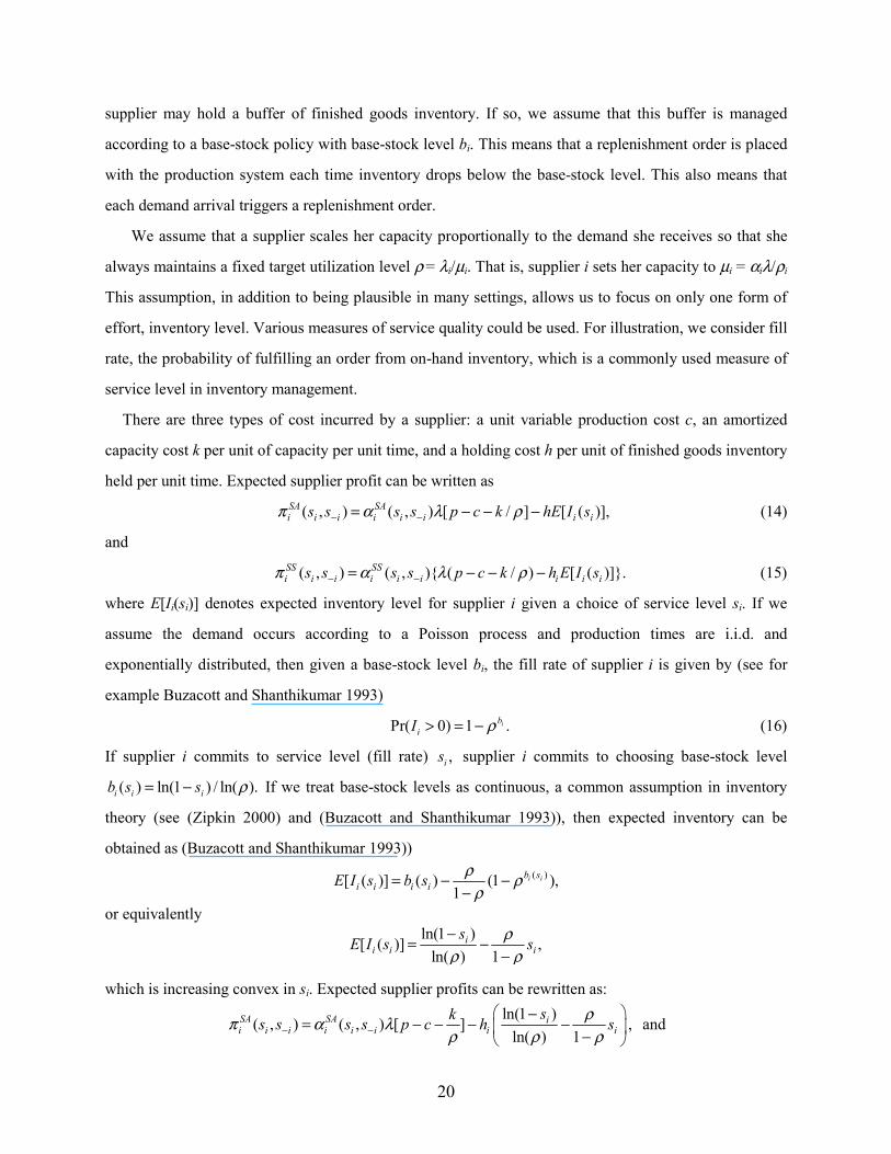
supplier may hold a buffer of finished goods inventory. If so, we assume that this buffer is managed

according to a base-stock policy with base-stock level bi. This means that a replenishment order is placed

with the production system each time inventory drops below the base-stock level. This also means that

each demand arrival triggers a replenishment order.

We assume that a supplier scales her capacity proportionally to the demand she receives so that she

always maintains a fixed target utilization level ρ = λi/µi. That is, supplier i sets her capacity to µi = αiλ/ρi

This assumption, in addition to being plausible in many settings, allows us to focus on only one form of

effort, inventory level. Various measures of service quality could be used. For illustration, we consider fill

rate, the probability of fulfilling an order from on-hand inventory, which is a commonly used measure of

service level in inventory management.

There are three types of cost incurred by a supplier: a unit variable production cost c, an amortized

capacity cost k per unit of capacity per unit time, and a holding cost h per unit of finished goods inventory

held per unit time. Expected supplier profit can be written as

( , ) ( , ) [ / ] [ ( )],SA SAi i i i i i i is s s s p c k hE I sπ α λ ρ− −= − − − (14)

and

( , ) ( , ){ ( / ) [ ( )]}.SS SSi i i i i i i i is s s s p c k h E I sπ α λ ρ− −= − − − (15)

where E[Ii(si)] denotes expected inventory level for supplier i given a choice of service level si. If we

assume the demand occurs according to a Poisson process and production times are i.i.d. and

exponentially distributed, then given a base-stock level bi, the fill rate of supplier i is given by (see for

example Buzacott and Shanthikumar 1993)

Pr( 0) 1 .ibiI ρ> = − (16)

If supplier i commits to service level (fill rate) ,is supplier i commits to choosing base-stock level

( ) ln(1 ) / ln( ).i i ib s s ρ= − If we treat base-stock levels as continuous, a common assumption in inventory

theory (see (Zipkin 2000) and (Buzacott and Shanthikumar 1993)), then expected inventory can be

obtained as (Buzacott and Shanthikumar 1993)) ( )[ ( )] ( ) (1 ),

1i ib s

i i i iE I s b s ρ ρρ

= − −−

or equivalently ln(1 )[ ( )] ,

ln( ) 1i

i i isE I s sρ

ρ ρ−

= −−

which is increasing convex in si. Expected supplier profits can be rewritten as: ln(1 )( , ) ( , ) [ ] ,

ln( ) 1SA SA ii i i i i i i i

sks s s s p c h sρπ α λρ ρ ρ− −

� �−= − − − −� �−� �

and

21

ln(1 )( , ) ( , ){ ( ) }.ln( ) 1

SS SS ii i i i i i i i

sks s s s p c h sρπ α λρ ρ ρ− −

� �−= − − − −� �−� �

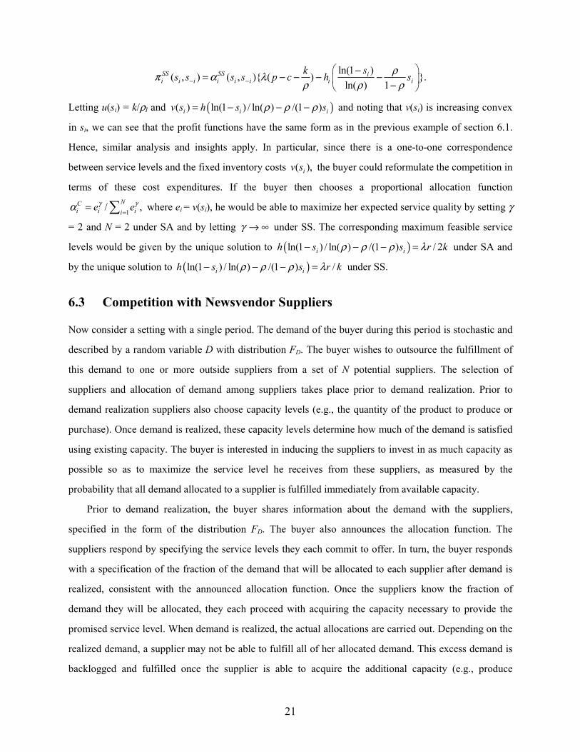
Letting u(si) = k/ρI and ( )( ) ln(1 ) / ln( ) /(1 )i i iv s h s sρ ρ ρ= − − − and noting that v(si) is increasing convex

in si, we can see that the profit functions have the same form as in the previous example of section 6.1.

Hence, similar analysis and insights apply. In particular, since there is a one-to-one correspondence

between service levels and the fixed inventory costs ( ),iv s the buyer could reformulate the competition in

terms of these cost expenditures. If the buyer then chooses a proportional allocation function

1/ ,NCi i iie eγ γα == � where ei = v(si), he would be able to maximize her expected service quality by setting γ

= 2 and N = 2 under SA and by letting γ → ∞ under SS. The corresponding maximum feasible service

levels would be given by the unique solution to ( )ln(1 ) / ln( ) /(1 ) / 2i ih s s r kρ ρ ρ λ− − − = under SA and

by the unique solution to ( )ln(1 ) / ln( ) /(1 ) /i ih s s r kρ ρ ρ λ− − − = under SS.

6.3 Competition with Newsvendor Suppliers

Now consider a setting with a single period. The demand of the buyer during this period is stochastic and

described by a random variable D with distribution FD. The buyer wishes to outsource the fulfillment of

this demand to one or more outside suppliers from a set of N potential suppliers. The selection of

suppliers and allocation of demand among suppliers takes place prior to demand realization. Prior to

demand realization suppliers also choose capacity levels (e.g., the quantity of the product to produce or

purchase). Once demand is realized, these capacity levels determine how much of the demand is satisfied

using existing capacity. The buyer is interested in inducing the suppliers to invest in as much capacity as

possible so as to maximize the service level he receives from these suppliers, as measured by the

probability that all demand allocated to a supplier is fulfilled immediately from available capacity.

Prior to demand realization, the buyer shares information about the demand with the suppliers,

specified in the form of the distribution FD. The buyer also announces the allocation function. The

suppliers respond by specifying the service levels they each commit to offer. In turn, the buyer responds

with a specification of the fraction of the demand that will be allocated to each supplier after demand is

realized, consistent with the announced allocation function. Once the suppliers know the fraction of

demand they will be allocated, they each proceed with acquiring the capacity necessary to provide the

promised service level. When demand is realized, the actual allocations are carried out. Depending on the

realized demand, a supplier may not be able to fulfill all of her allocated demand. This excess demand is

backlogged and fulfilled once the supplier is able to acquire the additional capacity (e.g., produce

22

additional units). Depending on the realized demand, a supplier may also be left with excess capacity

whose salvage price we assume is zero. Although all the demand that is allocated to a supplier is

eventually satisfied, the buyer is interested in minimizing the delays that result from backlogging.

Therefore, the buyer is interested in inducing the suppliers to invest in as much initial capacity as

possible. In contrast, suppliers are interested in minimizing their risk and would prefer to invest as little

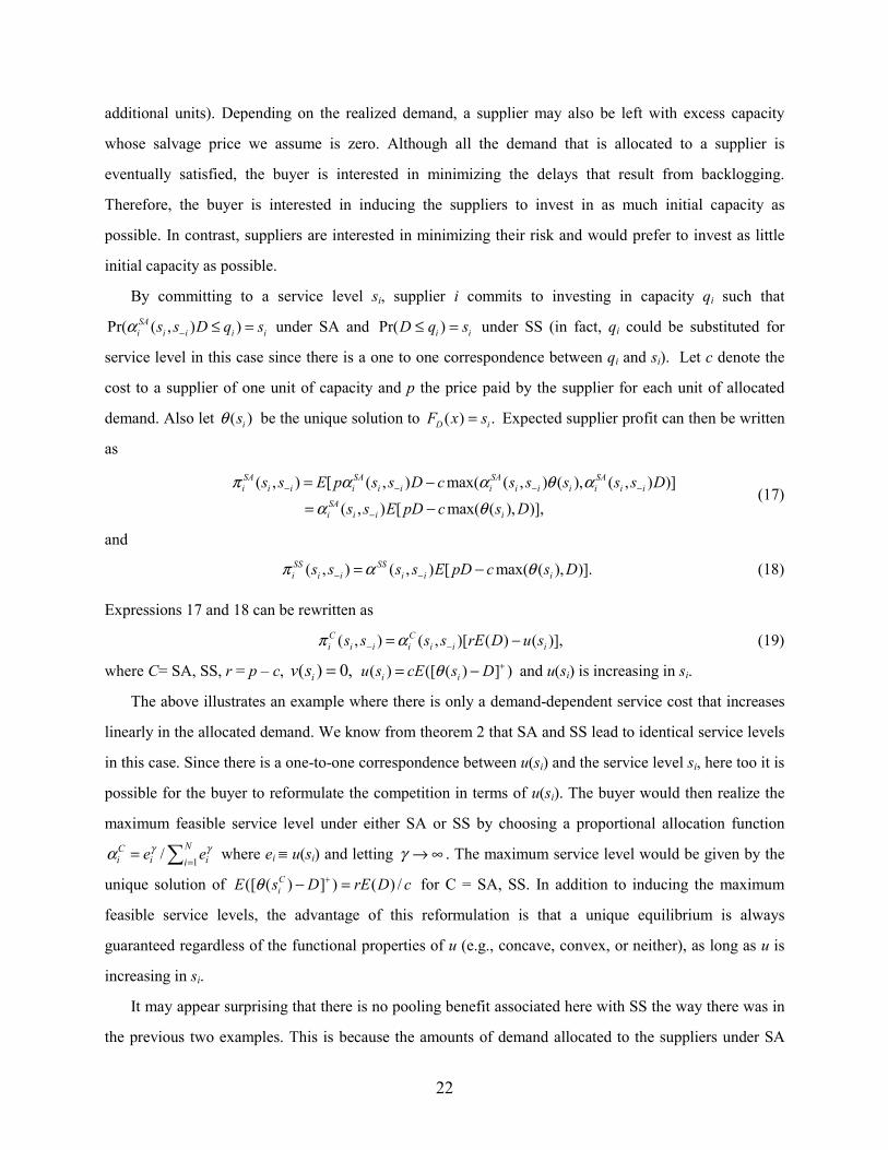
initial capacity as possible.

By committing to a service level si, supplier i commits to investing in capacity qi such that

Pr( ( , ) )SAi i i i is s D q sα − ≤ = under SA and Pr( )i iD q s≤ = under SS (in fact, qi could be substituted for

service level in this case since there is a one to one correspondence between qi and si). Let c denote the

cost to a supplier of one unit of capacity and p the price paid by the supplier for each unit of allocated

demand. Also let ( )isθ be the unique solution to ( ) .D iF x s= Expected supplier profit can then be written

as

( , ) [ ( , ) max( ( , ) ( ), ( , ) )]

( , ) [ max( ( ), )],

SA SA SA SAi i i i i i i i i i i i i

SAi i i i

s s E p s s D c s s s s s Ds s E pD c s D

π α α θ αα θ

− − − −

−

= −

= − (17)

and

( , ) ( , ) [ max( ( ), )].SS SSi i i i i is s s s E pD c s Dπ α θ− −= − (18)

Expressions 17 and 18 can be rewritten as

( , ) ( , )[ ( ) ( )],C Ci i i i i i is s s s rE D u sπ α− −= − (19)

where C= SA, SS, r = p – c, ( ) 0,iv s = ( ) ([ ( ) ] )i iu s cE s Dθ += − and u(si) is increasing in si.

The above illustrates an example where there is only a demand-dependent service cost that increases

linearly in the allocated demand. We know from theorem 2 that SA and SS lead to identical service levels

in this case. Since there is a one-to-one correspondence between u(si) and the service level si, here too it is

possible for the buyer to reformulate the competition in terms of u(si). The buyer would then realize the

maximum feasible service level under either SA or SS by choosing a proportional allocation function

1/ NCi i iie eγ γα == � where ei ≡ u(si) and letting γ → ∞ . The maximum service level would be given by the

unique solution of ([ ( ) ] ) ( ) /CiE s D rE D cθ +− = for C = SA, SS. In addition to inducing the maximum

feasible service levels, the advantage of this reformulation is that a unique equilibrium is always

guaranteed regardless of the functional properties of u (e.g., concave, convex, or neither), as long as u is

increasing in si.

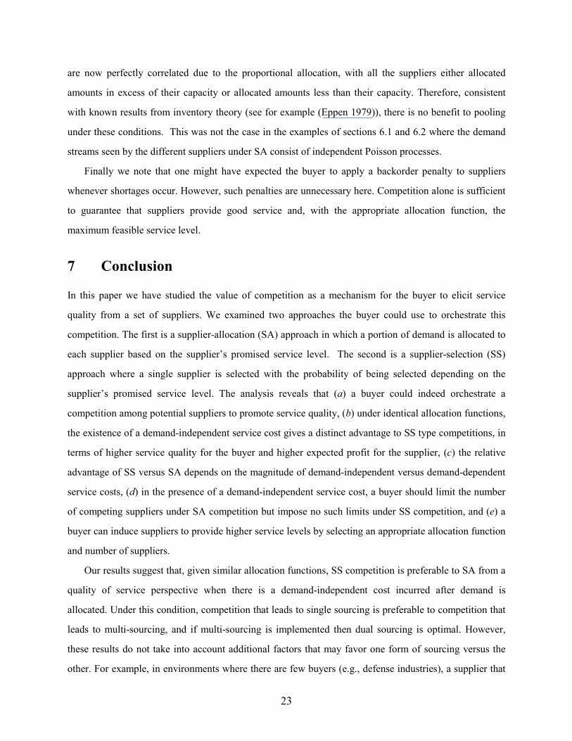
It may appear surprising that there is no pooling benefit associated here with SS the way there was in

the previous two examples. This is because the amounts of demand allocated to the suppliers under SA

23

are now perfectly correlated due to the proportional allocation, with all the suppliers either allocated

amounts in excess of their capacity or allocated amounts less than their capacity. Therefore, consistent

with known results from inventory theory (see for example (Eppen 1979)), there is no benefit to pooling

under these conditions. This was not the case in the examples of sections 6.1 and 6.2 where the demand

streams seen by the different suppliers under SA consist of independent Poisson processes.

Finally we note that one might have expected the buyer to apply a backorder penalty to suppliers

whenever shortages occur. However, such penalties are unnecessary here. Competition alone is sufficient

to guarantee that suppliers provide good service and, with the appropriate allocation function, the

maximum feasible service level.

7 Conclusion

In this paper we have studied the value of competition as a mechanism for the buyer to elicit service

quality from a set of suppliers. We examined two approaches the buyer could use to orchestrate this

competition. The first is a supplier-allocation (SA) approach in which a portion of demand is allocated to

each supplier based on the supplier’s promised service level. The second is a supplier-selection (SS)

approach where a single supplier is selected with the probability of being selected depending on the

supplier’s promised service level. The analysis reveals that (a) a buyer could indeed orchestrate a

competition among potential suppliers to promote service quality, (b) under identical allocation functions,

the existence of a demand-independent service cost gives a distinct advantage to SS type competitions, in

terms of higher service quality for the buyer and higher expected profit for the supplier, (c) the relative

advantage of SS versus SA depends on the magnitude of demand-independent versus demand-dependent

service costs, (d) in the presence of a demand-independent service cost, a buyer should limit the number

of competing suppliers under SA competition but impose no such limits under SS competition, and (e) a

buyer can induce suppliers to provide higher service levels by selecting an appropriate allocation function

and number of suppliers.

Our results suggest that, given similar allocation functions, SS competition is preferable to SA from a

quality of service perspective when there is a demand-independent cost incurred after demand is

allocated. Under this condition, competition that leads to single sourcing is preferable to competition that

leads to multi-sourcing, and if multi-sourcing is implemented then dual sourcing is optimal. However,

these results do not take into account additional factors that may favor one form of sourcing versus the

other. For example, in environments where there are few buyers (e.g., defense industries), a supplier that

24

does not receive an allocation could go out of business. In that case, the buyer needs to support multiple

suppliers to ensure continued competition in the future. A decision on the part of the buyer to single, dual

or multi-source should trade off service quality benefits with these other tangible and less tangible

benefits. In fact, our results are most useful for separately documenting the impact of different parameters

on the performance of each type of competition. Finally, our results show that the differences between SA

and SS depend on the timing of when the demand-independent costs are incurred. In particular, if the

independent costs are incurred prior to the demand allocation under SA and prior to supplier selection

under SS, SA and SS are equivalent in terms of the expected service level they yield to the buyer.

Our results comparing SA and SS can be recast as a comparison between two forms of SS

competition, one with demand-independent costs incurred prior to demand allocation and one with

demand-independent costs incurred post demand allocation. These results could be extended to examine

settings where demand-independent costs are incurred in two stages: one portion occurring pre-allocation

and the other post allocation. In practice, pre-allocation costs may be desirable since they could reduce the

risk of a supplier reneging on the promised service levels. However, this risk-mitigation benefit needs to

be balanced against the service level reduction it induces.

There are several possible avenues for future research. Our analysis currently relies on the assumption

of identical service cost functions among suppliers. Dropping this assumption would allow us to consider

situations where some suppliers are more cost efficient than others. The degree of cost asymmetry could

affect the behavior and performance of our two types of competition, as well as the type of allocation

functions that maximize service quality. Allocation functions that intensify competition could lead under

SA to a small number of suppliers capturing most of the demand. With asymmetry, it is also not clear if

there would always be allocation functions that lead to zero supplier profits. In highly asymmetric

settings, the most cost-effective supplier could capture most of the demand while expending only a

fraction of her revenue on service cost.

We have also assumed that the set of participating suppliers is exogenously determined. However,

one could consider the joint decision of choosing M suppliers out of the pool of N and then allocating

demand among these M winners. SA and SS are actually special cases of this more general problem, with

SA implying M = N and SS implying M = 1. Under this generalized scheme, the buyer decides on both a

selection function to determine the M winners and an allocation function to determine how demand is

divided. This generalized form of the competition could capture benefits of both SA and SS. For example,

by choosing a large value for N the buyer (with appropriate choice of selection and allocation functions)

25

may be able to intensify the competition and extract high service levels while still maintaining multiple

suppliers, which might be desirable to management for reasons other than service quality. However, we

suspect that the effect of M, the number of suppliers that are eventually selected, would remain the same.

In particular, smaller M leads to higher service quality with the highest service quality realized when M =

1.

In certain settings, the buyer may not be interested in maximizing the average service quality received

from his suppliers. Instead, the buyer may be interested in measures of service that depend in different

ways on the effort profile of the various suppliers. For example, the buyer could be interested in

cumulative expenditures by the suppliers (e.g., total capacity investments in the supply chain).

Alternatively, the buyer could be interested in reducing the variance of service levels across different

suppliers (e.g., minimizing maximum delay over all suppliers). We expect different service measures to

favor different types of competition. For example, we know that SA induces a lower average service level

but a higher total cost expenditures on service. Therefore when buyers care about cumulative

expenditures, SA becomes superior and multi-sourcing more desirable.

Finally, our analysis could be extended to settings where the buyer may choose to outsource only a

fraction of her demand under SA or reserve the right not to select any suppliers under SS. This could be

implemented by the buyer by choosing for example an allocation function of the form

1( , ) ( )NCi i i i iis s s sα κ− == +� where κ > 0 (see Elahi (2006) for further discussion). Under SA, the

fraction 1( )Nii sκ κ =+� corresponds to the fraction of demand that is not allocated to any supplier, while

under SA the same fraction corresponds to the probability that no supplier is selected. The parameter κ

could correspond to a known service level offered by an incumbent (current) supplier or to the service

level realized if the buyer decides to produce in-house. We expect the threat of partial outsourcing to

affect the outcome of the competition. In cases where the buyer can choose the parameter κ, we also

suspect there may be values of this parameter that maximize the service levels received from the

suppliers.

Acknowledgments: We are grateful to the Associate Editor and two anonymous reviewers for many helpful comments and suggestions. We also wish to thank seminar participants at the following universities: Chicago, Cornell, Hong-Kong, Koç, Purdue and USC for many insightful questions and comments that led to improvements in our analysis. This research is supported by the National Science Foundation through grant DMI-0500381.

26

References Allon, G. and A. Federgruen, “Competition in Service Industries,” working paper, Columbia University, 2005. Anton, J. J. and D. A. Yao, “Split Awards, Procurement, and Innovation,” RAND Journal of Economics, 20, 538-552, 1989. Anupindi, R. and R. Akella, “Diversification under Supply Uncertainty”, Management Science, 39, 944-963, 1993. Benjaafar, S., William L. Cooper and J. S. Kim, “On the Benefits of Pooling in Production-Inventory Systems,” Management Science, 51, 548-565, 2005. Bell, D., R. Keeney and J. Little, “A Market Share Theorem,” Journal of Marketing Research, 12, 136-141, 1975. Bernstein, F. and A. Federgruen, “A General Equilibrium Model for Industries with Price and Service Competition,” Operations Research, 52, 868-886, 2004. Boyaci, T. and G. Gallego, “Supply Chain Coordination in a Market with Customer Service Competition,” Production and Operations Management, 13, 3-22, 2004. Boyaci, T. and S. Ray, “Product Differentiation and Capacity Cost Interaction in Time and Price Sensitive Markets,” Manufacturing Service and Operations Management, 5, 18-36, 2003. Buzacott J. A. and G. Shanthikumar, Stochastic Models of Manufacturing Systems, Prentice Hall, 1993. Cachon, G. P., “Supply Chain Coordination with Contracts,” in Handbooks in Operations Research and Management Science: Supply Chain Management, editors: S. Graves and T. de Kok, North-Holland, 2003. Cachon, G. P. and F. Zhang, “Obtaining Fast Service in a Queueing System via Performance-Based Allocation of Demand,” working paper, The Wharton School, University of Pennsylvania, 2005. Cachon, G. P. and F. Zhang, “Procuring Fast Delivery: Sole Sourcing with Information Asymmetry,” Management Science (forthcoming), 2006. Chen, F., “Auctioning Supply Contracts”, working paper, Graduate School of Business, Columbia University, 2004. Chen, J., D. D. Yao, and S. Zheng, “Optimal Replenishment and Rework with Multiple Unreliable Supply Sources,” Operations Research, 49, 430-443, 2001. Cooper, L.G., “Marketing Share Models,” Chapter 6 in (Eliashberg and Lilien, 1993). Dixit, A., “Strategic Behavior in Contests,” American Economic Review, 77, 891-898, 1987. Elahi, E., Orchestrating Supplier Competition, Ph.D. Thesis, University of Minnesota, 2006.

27

Elahi, E., Benjaafar, S. and K. Donohue “Inventory Competition in Make-to-Stock Systems,” working paper, University of Minnesota, 2003. Elmaghraby, W. J., “Supply Contract Competition and Sourcing Strategies,” Manufacturing Service and Operations Management, 2, 350-371, 2000. Eliashberg, J. And G.L. Lilien (editors), Marketing, Volume 5 of Handbooks in OR/MS, North Holland, 1993. Eppen, G. D., “Effects of Centralization on Expected Costs in a Multi-Location Newsboy Problem,” Management Science, 25 498–501, 1979. Farlow, D., G. Schmidt, A. Tsay, “Supplier Management at Sun Microsystems,” Stanford Business School Case, 1996. Fong, D. K. H., V. M. Gempesaw and J. K. Ord, “Analysis of a Dual Sourcing Inventory Model with Normal Unit Demand and Erlang Mixture Lead Times,” European Journal of Operational Research, 120, 97-107, 2000. Fudenberg, D. and J. Tirole, Game Theory, MIT Press, 1991. Gans, N., “Customer Loyalty and Supplier Quality Competition,” Management Science, 48, 207-221, 2002. Gilbert, S. and Z. K. Weng, “Incentive Effects Favor Non-Competing Queues in a Service System: the Principal-Agent Perspective,” Management Science, 44, 1662-1669, 1997. Green, J. R. and N. L. Stokey, “A Comparison of Tournaments and Contracts,” Journal of Political Economy, 91, 349-364, 1983. Ha, A. Y., Personal communication, Hong Kong University of Science and Technology, 2004. Ha, A.Y., L. Li, and S. M. Ng, “Price and Delivery Logistics Competition in a Supply Chain,” Management Science, 49, 1139-1153, 2003. Hall, J. and E. Porteus, “Customer Service Competition in Capacitated Systems,” Manufacturing Service and Operations Management, 2, 144-165, 2000. Kalai, E., M. Kamien and M. Rubinovitch, “Optimal Service Speeds in a Competitive Environment,” Management Science, 38, 1154-1163, 1992. Kalra, A. and M. Shi, “Designing Optimal Sales Contests: A Theoretical Perspective,” Marketing Science, 20, 170-193, 2001. Karjalainen, R, “The Newsboy Game,” working paper, Wharton School, University of Pennsylvania, 1992. Klemperer, P., “Auction Theory: A Guide to the Literature,” Journal of Economics Surveys, 13, 227-286, 1999. Konrad, K. and Schlesinger, H., “Risk-Aversion in Rent-Seeking and Rent-Augmenting Games,” The Economic Journal, 107, 1671-1683, 1997.

28

Kotler, P., Marketing Management: Analysis, Planning and Control, 5th ed., Prentice-Hall, 1984. Laffont, J. and J. Tirole, A Theory of Incentives in Procurement and Regulation, MIT Press, 1994. Lazear, E. P. and S. Rosen, “Rank-Order Tournaments as Optimum Labor Contracts,” Journal of Political Economy, 89, 841-864, 1981. Li, Q. and A. Y. Ha, “Accurate Response, Reactive Capacity and Inventory Competition,” Working paper, Hong Kong University of Science and Technology, 2003. Lilien G., P. Kotler and S. Moorthy, Marketing Models, Prentice Hall, New Jersey, 1992. Lippman, S. A. and K. F. McCardle, “The Competitive Newsboy,” Operations Research, 45, 54-65, 1997. Mahajan S. and G. Van Ryzin, “Inventory Competition under Dynamic Consumer Choice,” Operations Research, 49, 646-657, 2001a. Mahajan, S. and G. van Ryzin, “A Stocking Retail Assortments under Dynamic Consumer Substitution,” Operations Research, 49, 334-351, 2001b. McAfee, R.P. and J. McMillan, “Auctions and Bidding,” Journal of Economics Literature, 25, 699-738, 1987. Moinzadeh, K. and S. Nahmias, “A Continuous Review Model for an Inventory System with Two Supply Modes,” Management Science, 26, 483-494. 1988. Monahan, G.E., “The Structure of Equilibria in Market Share Attraction Models,” Management Science, 33, 228-243, 1987. Monahan, G. E. and M. Sobel, “Risk-Sensitive Dynamic Market Share Attraction Games,” Games and Economic Behavior, 20,149-160, 1997. Moorthy, K.S., “Competitive Marketing Strategies: Game-Theoretic Models”, Chapter 4 in (Eliashberg and Lilien, 1993). Netessine, S. and N. Rudi, “Centralized and Competitive Inventory Models with Demand Substitution,” Operations Research, 51, 329-335, 2003. Nitzan, S., “Modelling Rent-Seeking Contests,” European Journal of Political Economy, 10, 41-60, 1994. Nti, K. O., “Comparative Statics of Contests and Rent-Seeking Games,” International Economic Review, 38, 43-59, 1997. Normile, D., “Taiwan's United Microelectronics Corp. Looks to Partnerships to Improve its Foundry Business,” Electronic Business Magazine, November, 2003. Parlar, M, “Game Theoretic Analysis of the Substitutable Product Inventory Problem with Random Demands,” Naval Research Logistics, 35, 397-409, 1988.

29

PeopleSoft, “PeopleSoft Supplier Rating System,” Promotional material available for download from www.peoplesoft.com, 2004. Perez-Castrillo, J. D. and Verdier, T., ‘‘A General Analysis of Rent-Seeking Games,’’ Public Choice, 73, 335-350, 1992. Ramasesh, R.V., J. K. Ord, J .C. Hayya and A. C. Pan Pan, “Sole versus Dual Sourcing in Stochastic Lead-Time (s, Q) Inventory Models,” Management Science, 37, 428-443, 1991. Roberts, B., “Top 100 Contract Manufacturers,” Electronic Business Magazine, September, 2003. Rosenblatt, M. J., Y. T. Herer, and I. Hefter, “Note. An Acquisition Policy for a Single Item Multi-Supplier System,” Management Science, 44, S96-S100, 1998. Ross, C. F., R. Shevlin and L. Herbert, “2003: Financial Services Outsourcing Will Grow 10%,” Forester Research Report, 2003. Seshadri, S., “Bidding for Contests,” Management Science, 41, 561- 576, 1995. Seshadri, S. and E. Zemel, “Supply Intelligence”, working paper, Stern School of Business, New York University, 2003. Skaperdas, S., “Contest Success Functions,” Economic Theory, 7, 283-290, 1996. Swaminathan, J. M. and J. G. Shanthikumar, “Supplier Diversification: Effect of Discrete Demand,” Operations Research Letters, 24, 213-221, 1991. Talluri, K. and G.J. van Ryzin. The Theory and Practice of Revenue Management, Kluwer Academic Publishers, 2004. Tullock, G., “Rent-Seeking as a Negative-Sum Game,” in Toward a Theory of the Rent-Seeking Society, edited by J. M. Buchanan, R. D. Tollison and G. Tullock, Texas A&M University Press, 97-112, 1980. Wang, Y. and Y. Gerchak, “Supply Chain Coordination When Demand is Shelf-Space Dependent,” Manufacturing & Service Operations Management, 3, 82-87, 2001. Whittmore, A. S. and S. Saunders, “Optimal Inventory Under Stochastic Demand With Two Supply Options,” SIAM Journal of Applied Mathematics, 32, 293-305, 1977. Zipkin P. H., Foundations of Inventory Management, McGraw-Hill, New York, 2000.

30

Appendix

Proof of theorem 1 We first note that the decision space for each supplier i=1, …, N is given by [0, ]us , where us is the

unique solution of ( ,0) 0ir f sλ − = for the case of SA competition and ( , ) 0ir f sλ λ− = for the case of

SS competition. The service level us is finite since f is increasing convex.

SA competition

It can be easily shown that the profit function of supplier i is concave with respect to si, i=1,…,N. Therefore, a Nash equilibrium can be obtained as the solution to the following system of N first order optimality condition equations:

( )( , ) ( , ) ( ) ( )( ) 0SA SA

SAi i i i i i i ii i

i i i i

s s s s u s v sr u ss s s s

π α λ α λ− − � �∂ ∂ ∂ ∂= − − + =� �∂ ∂ ∂ ∂� �

for i=1,.., N, (A1)

or equivalently

( )( )1

211

( ) ( ) ( )( ) ( ) ( ) ( ) 0( )( )

Ni ii i

i i i iNNiiii

g s g s g sg s r u s u s v sg sg s

λ λ=

==

� �−� �′ ′ ′− − + =� �� �

�

�� for i=1,.., N. (A2)

Let sSA > 0 be the unique solution to the following equation:

( )21 1( ) ( ) ( ) ( ) 0.

( )N g s r u s u s v s

NN g sλ λ− � �′ ′ ′− − + =� �� �

(A3)

Also, let ( ) 2( ) ( 1) ( ) ( ) / ( )SAA s N g s r u s N g sλ′= − − and ( ) ( ) / ( )SAB s u s N v sλ ′ ′= + . Therefore, A3 can be written as ( ) ( ) 0SA SAA s B s− = . This equation has a unique strictly positive solution since (a) 0lim ( ) ,SA

s A s→ = +∞ (b) 0( ) 0SAA s = , where s0 is the solution to 0( );r u s= furthermore, ( ) 0SAA s = does not admit any other solution, (c) the positive part of ( )SAA s is decreasing in s, (d) (0) 0,SAB ≥ (e) ( )SAB s is non-decreasing in s, and (f) ( )SAB s >0 for s>0. It is easy to check that si= sSA, i=1,…, N is a solution to the system of equations A2. Hence, to complete the proof of the theorem, it only remains to show that there cannot be another solution to A2, which implies that si= sSA, for i=1, …, N, is the unique Nash equilibrium. The following system of N+1 equations with unknowns si and G is equivalent to the system of equations A2:

( )2( ) ( )( ) ( ) ( ) ( ) 0i i

i i i iG g s g sg s r u s u s v s

GGλ λ− � �′ ′ ′− − + =� �

� �, for i = 1,…, N and (A4)

31

1 ( ) 0Nii g s G= − =� . (A5)

By virtue of lemma A1 below, each equation in A4 admits at most one positive solution in the decision space of each supplier. Therefore, si = sSA for i = 1,…, N and G =Ng(sSA) is the only solution for the system of equations A4-A5.

Lemma A1: Let ( ) ( )2( , ) ( ( )) / ( ) ( ) ( ) / ( ) ( )SAi i i i i i i is G G g s G g s r u s g s G u s v sφ λ λ� � ′ ′ ′� �= − − − +� �� � where G >

0 is a constant, ( ) ( ) /i i ig s g s s′ = ∂ ∂ , ( ) ( ) /i i iu s u s s′ = ∂ ∂ , and ( ) ( ) /i i iv s v s s′ = ∂ ∂ . Then equation

( , ) 0SAi is Gφ = admits at most one strictly positive solution in the decision space of supplier i.

Proof: Let ,1 ,2( , ) ( , ) ( , )SAi i i i i is G s G s Gφ φ φ= − , where

( )2,1( , ) ( ( )) / ( ) ( )i i i i is G G g s G g s r u sφ λ� � ′= − −� � and ( ),2 ( , ) ( ) / ( ) ( )i i i i is G g s G u s v sφ λ ′ ′� �= +� � .

We know that (a) since u(si) is an increasing convex function there is at least one finite solution to equation

,1( , ) 0i is Gφ = , let si,0 be the smallest solution to this equation, (b) ,1(0, ) 0,i Gφ > (c) ,1( , )i is Gφ is decreasing in ,0[0, ],i is s∈ and (d) ,2 ( , )i is Gφ is non-negative and increasing in si. Consequently, equation ( , ) 0SA

i is Gφ = admits a unique positive solution in ,0[0, ]is if (0, ) 0SAi Gφ ≥ .

Otherwise, it admits no solution. We also notice that the term ( )( )ir u s− in ,1iφ is always non-negative for ˆ[0, ]i is s∈ , where is is the unique solution to ( )( ) 0ir u s− = . Therefore, ,1 0iφ = cannot admit more than one solution in this interval. As a result, ( , ) 0SA

i is Gφ = cannot have more than one solution in ˆ[0, ].is Since for ˆi is s> the profit of supplier i is negative we can conclude that ˆ[0, ]is contains the decision space of supplier i. This completes the proof of the lemma. SS competition It can be easily shown that the profit function of supplier i is concave with respect to si, i=1,…,N. Therefore, a Nash equilibrium can be obtained as the solution to the following system of N first order optimality condition equations:

( )( , ) ( , ) ( ) ( )( ) ( ) 0SS SS

SSi i i i i i i ii i i

i i i i

s s s s u s v sr u s v ss s s s

π α λ λ α λ− − � �∂ ∂ ∂ ∂= − − − + =� �∂ ∂ ∂ ∂� �

for i=1,.., N, (A6)

or equivalently

( )( ) ( )1

211

( ) ( ) ( )( ) ( ) ( ) ( ) ( ) 0( )( )

Ni ii i

i i i i iNNiiii

g s g s g sg s r u s v s u s v sg sg s

λ λ λ λ=

==

−′ ′ ′− − − + =�

�� for i=1,.., N. (A7)

Let sSS > 0 be the unique solution to the following equation:

( ) ( )21 1( ) ( ) ( ) ( ) ( ) 0.

( )N g s r u s v s u s v s

NN g sλ λ λ− ′ ′ ′− − − + = (A8)

32

Also, let ( ) 2( ) ( 1) ( ) ( ) ( ) / ( )SSA s N g s r u s v s N g sλ λ′= − − − and ( )( ) ( ) ( ) /SSB s u s v s Nλ ′ ′= + . Therefore, A9 can be written as ( ) ( ) 0.SS SSA s B s− = This equation has a unique strictly positive solution since (a) 0lim ( ) ,SS

s A s→ = +∞ (b) 0( ) 0SSA s = , where s0 is the solution to 0 0( ) ( ) 0;r u s v sλ λ− − = furthermore, ( ) 0SSA s = does not

admit any other solution, (c) the positive part of ( )SSA s is decreasing in s, (d) (0) 0,SSB ≥ (e) ( )SSB s is non-decreasing in s, and (f) ( )SSB s >0 for s>0. It is easy to check that si = sSS for i = 1,…, N is a solution to the system of equations A7. Hence, to complete the proof of the theorem, we only need to show that there cannot be another solution to A7.

The following system of N+1 equations with unknowns si and G is equivalent to the system of

equations A8.

( ) ( )2( ) ( )( ) ( ) ( ) ( ) ( ) 0i i

i i i i iG g s g sg s r u s v s u s v s

GGλ λ λ− ′ ′ ′− − − + = , for i=1,…, N, and (A9)

1 ( ) 0Nii g s G= − =� . (A10)

By virtue of lemma A2 below, each equation in A10 admits at most one positive solution in the decision space of each supplier. Therefore, si = sSS, i=1,…,N and G =Ng(sSS) is the only solution for the system of equations A9-A10.

Lemma A2: Let

( ) ( )( )2( , ) ( ( )) / ( ) ( ) ( ) ( ) / ( ) ( )SSi i i i i i i i is G G g s G g s r u s v s g s G u s v sφ λ λ λ� � ′ ′ ′� �= − − − − +� �� � ,

where G > 0 is a constant, ( ) ( ) /i i ig s g s s′ = ∂ ∂ , ( ) ( ) /i i iu s u s s′ = ∂ ∂ , and ( ) ( ) /i i iv s v s s′ = ∂ ∂ . Then equation ( , ) 0SS

i is Gφ = admits at most one strictly positive solution in the decision space of supplier i.

Proof: Let ,1 ,2( , ) ( , ) ( , )SSi i i i i is G s G s Gφ φ φ= − , where

( )2,1( , ) ( ( )) / ( ) ( ) ( )i i i i i is G G g s G g s r u s v sφ λ λ� � ′= − − −� � and

( )( ),2 ( , ) ( ) / ( ) ( )i i i i is G g s G u s v sφ λ ′ ′� �= +� � .

We know that

(a) since u(si) and v(si) are an increasing convex functions there is at least one finite solution to equation

,1( , ) 0;i is Gφ = let si,0 be the smallest solution to this equation,

(b) ,1(0, ) 0i Gφ > ,

(c) ,1( , )i is Gφ is decreasing in ,0[0, ]i is s∈ , and

(d) ,2 ( , )i is Gφ is non-negative and increasing in si with ,2 (0, ) 0i Gφ = .

Consequently, equation ( , ) 0SSi is Gφ = admits a unique positive solution in ,0[0, ].is Note also that the

term ( )( ) ( )i ir u s v sλ λ− − in ,1iφ is always non-negative in the decision space of supplier i, [0, ]uis where

33

uis is defined in the proof of theorem 1. Therefore, ,1 0iφ = cannot admit more than one solution in this

interval. As a result, ( , ) 0i is Gφ = cannot have more than one solution in [0, ]uis .

Proof of Theorem 2 Result (1)

The result is obvious since the profit functions of SA and SS competitions have the same form.

Result (2)

First recall that the Nash equilibria for SA and SS competitions are, respectively, the solutions to the following equations:

SA: ( )21 1( ) ( ) ( ) '( )

( )N g s r u s u s v s

NN g sλ λ− � �′ ′− = +� �

� � and (A11)

SS: ( )1 ( ) ( ) ( ) ( ) ( ),( )

N g s r u s v s u s v sNg s

λ λ− ′ ′ ′� �− − = +� � (A12)

which can also be rewritten as

SA: ( ) [ ]( ) ( )( ) ( ) ( ) ( )( ) 1 ( )

g s N g sr u s N v s u s v sg s N g s

λ λ′ ′ ′− − = +′ ′−

, and (A13)

SS: ( ) ( )( )( ) ( ) ( ) ( ) .1 ( )

N g sr u s v s u s v sN g s

λ λ ′ ′− − = +′−

(A14)

In order to show that the solution to equation A13, sSA, is always less than the solution to equation A14, sSS, we state and prove the following set of claims.

Claim 1: For the functions g, u, and v, ( ) ( )g s g s s′ ≥ , ( ) ( )u s u s s′ ≤ , and ( ) ( )v s v s s′ ≤ . To verify claim 1, let ( ) ( ) ( )g s g s g s sθ ′= − , then (0) 0gθ = and

2 2

( ) ( ) ( ) ( ) ( ) ( ) ( )1 0.( ) ( )

gd s g s g s g s g s g s g sds g s g s

θ ′ ′ ′′ ′′− −= − = ≥′ ′

Therefore, ( ) ( ) ( ) 0g s g s g s sθ ′= − ≥ . Next, let ( ) ( ) ( ) ,u s u s u s sθ ′= − then (0) 0uθ = and

2 2( ) ( ) ( ) ( ) ( ) ( ) ( )1 0.

( ) ( )ud s u s u s u s u s u s u sds u s u s

θ ′ ′ ′′ ′′− −= − = ≤′ ′

Therefore, ( ) ( ) ( ) 0u s u s u s sθ ′= − ≤ . Similarly, we can show that ( ) ( ) ( ) 0v s v s v s sθ ′= − ≤ .

Claim 2: Let ( ) ( )1( ) ( ) ( ) / ( ) ( )s r u s N g s g s v sη λ ′ ′= − − and ( )2 ( ) ( ) ( )s r u s v sη λ= − − . For any s > 0 we have 2 1( ) ( )s sη η> . Claim 2 follows by noting that, by virtue of Claim 1, we have

( )2 1( ) ( ) ( ) / ( ) ( ) ( ) ( ) ( ) ( ) ( ) 0.s s N g s g s v s v s Nsv s v s Nv s v sη η ′ ′ ′− = − ≥ − ≥ − > Claim 3: Let ( )( )3( ) /( 1) ( ) / ( ) ( ) ( )s N N g s g s u s v sη λ′ ′ ′= − + , s1 be the unique solution of 3 2( ) ( )s sη η= , and s2

be the unique solution of 3 1( ) ( ),s sη η= then s2 < s1.

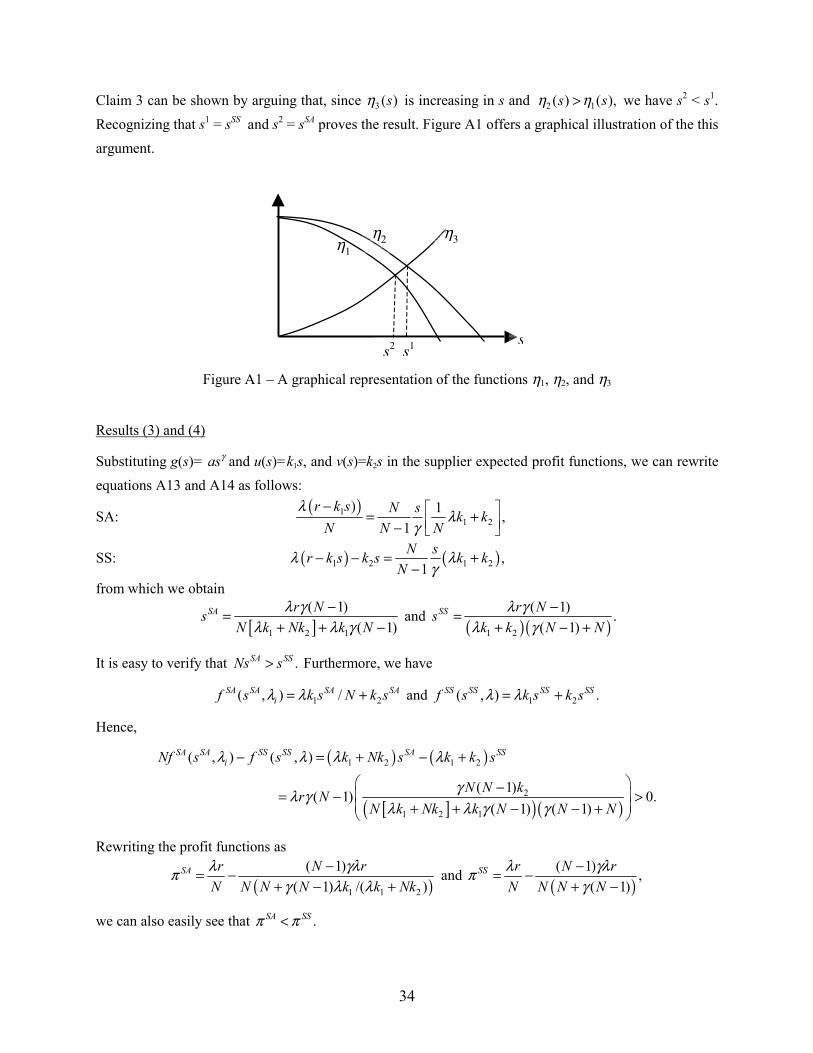
34

Claim 3 can be shown by arguing that, since 3 ( )sη is increasing in s and 2 1( ) ( ),s sη η> we have s2 < s1. Recognizing that s1 = sSS and s2 = sSA proves the result. Figure A1 offers a graphical illustration of the this argument.

Figure A1 – A graphical representation of the functions η1, η2, and η3

Results (3) and (4)

Substituting g(s)= asγ and u(s)=k1s, and v(s)=k2s in the supplier expected profit functions, we can rewrite equations A13 and A14 as follows:

SA: ( )11 2

) 1 ,1

r k s N s k kN N N

λλ

γ− � �= +� �− � �

SS: ( ) ( )1 2 1 2 ,1

N sr k s k s k kN

λ λγ

− − = +−

from which we obtain

[ ]1 2 1

( 1)( 1)

SA r NsN k Nk k N

λ γλ λ γ

−=+ + −

and ( )( )1 2

( 1) .( 1)

SS r Nsk k N N

λ γλ γ

−=+ − +

It is easy to verify that .SA SSNs s> Furthermore, we have

1 2( , ) /SA SA SA SAif s k s N k sλ λ= + and 1 2( , ) .SS SS SS SSf s k s k sλ λ= +

Hence,

( ) ( )

[ ]( )( )

1 2 1 2

2

1 2 1

( , ) ( , )

( 1) ( 1) 0.( 1) ( 1)

SA SA SS SS SA SSiNf s f s k Nk s k k s

N N kr NN k Nk k N N N

λ λ λ λ

γλ γλ λ γ γ

− = + − +

� �−� �= − >� �+ + − − +� �

Rewriting the profit functions as

( )1 1 2

( 1)( 1) /( )

SA r N rN N N N k k Nkλ γλπ

γ λ λ−= −

+ − + and ( )

( 1) ,( 1)

SS r N rN N N Nλ γλπ

γ−= −

+ −

we can also easily see that .SA SSπ π<

s2 s1

η1 η2 η3

s

35

Proof of Theorem 3 Result (1)

The Nash equilibrium service level is the solution to the following equation:

( )1 ( ) ( ) ( ) ( ) ( ).( )

N g s r u s v s u s v sNg s

λ λ λ− ′ ′ ′− − = + (A15)

Since, the right hand side is independent of N and increasing in s and the left hand side is increasing in N, the Nash equilibrium service level MSs is also increasing in N. Furthermore, since

( ) ( )1 ( )lim ( ) ( ) ( ) ( ) ( )( ) ( )N

N g sg s r u s v s r u s v sNg s g s

λ λ λ λ→∞′� �− ′ − − = − −� �

� �,

the Nash equilibrium service level approaches ,MSs the unique solution to

( )( ) ( ) ( ) / ( ) ( ) ( )g s r u s v s g s u s v sλ λ λ′ ′ ′− − = + . Since the solution is symmetric we have SS SSq s= . Result (2) When v(si)=0, the proof is similar to that of the result (1), and SA SAs q= is the solution to the following equation:

( )( ) ( ) / ( ) ( ).g s r u s g s u sλ λ λ′ ′− =

When ui(si)=0, the Nash equilibrium service level solves the following equation:

21 ( ) ( ).

( )N g s r v s

g sNλ′− ′=

The right hand side is independent of N and increasing in s, while the left hand side is decreasing in N. Consequently, the equilibrium point sSA is decreasing in N. Finally, since 1/SA

i Nα = and v(0) = 0, lim 0SA

N iπ→∞ = . For part (c), when both u(si) and v(si) are positive for si>0, the profit function is given by

( , ) ( , ) ( ( )) ( ).SA SAi i i i i i i is s s s r u s v sπ α λ− −= − −

Since SAiα approaches zero as N goes to infinity, the only service level which leads to a non-negative

profit is sSA= 0. In this case, the Nash equilibrium is the solution to

( )21 ( ) ( ) ( ) ( ).

( )N g s r u s u s v s

g s NNλλ′− ′ ′− = +

Noting that both sides of the above equation are decreasing in N, the right hand side is increasing in s, and the left hand side is decreasing in s, the solution to this equation is not necessarily increasing or decreasing in N. However, since the solution approaches zero as N goes to infinity it should be decreasing for large values of N.

Result (3)

Result (3) follows immediately from results (1) and (2).

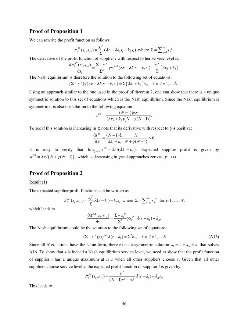
36

Proof of Proposition 1 We can rewrite the profit function as follows:

1 2( , ) ( )SS ii i i i i

ss s r k s k sγ

π λ λ− = − −Σ

where 1 .Njj s γ

=Σ =�

The derivative of the profit function of supplier i with respect to her service level is:

( )11 2 1 22

( , ) ( ) .SSi i i i i

i i ii

s s s ss r k s k s k ks

γ γγπ γ λ λ λ−−∂ Σ −

= − − − +∂ ΣΣ

The Nash equilibrium is therefore the solution to the following set of equations. ( )1 2 1 2( ) ( ) , for 1,..., .i i i is r k s k s k k s i Nγ γ λ λ λΣ − − − = Σ + =

Using an approach similar to the one used in the proof of theorem 2, one can show that there is a unique symmetric solution to this set of equations which is the Nash equilibrium. Since the Nash equilibrium is symmetric it is also the solution to the following equation:

( )1 2

( 1) .( ) ( 1)

SS N rsk k N N

γλλ γ

−=+ + −

To see if this solution is increasing in γ, note that its derivative with respect to γ is positive:

1 2

( 1) 0.( 1)

SSs N r Nk k N N

λγ λ γ

∂ −= >∂ + + −

It is easy to verify that 1 2lim /( )SSs r k kγ λ λ→∞ = + . Expected supplier profit is given by

( )/ ( 1) ,SS r N Nπ λ γ= + − which is decreasing in γ and approaches zero as γ → ∞ .

Proof of Proposition 2 Result (1)

The expected supplier profit functions can be written as

1 2( , ) ( )SA ii i i i

ss s r k k sγ

π λ− = − −Σ

where 1N

jj s γ=Σ =� for i=1, …, N,

which leads to 1

1 22( , ) ( ) .

SAi i i i

ii

s s s s r k ks

γγπ γ λ−−∂ Σ −

= − −∂ Σ

The Nash equilibrium could be the solution to the following set of equations: 1 2

1 2( ) ( ) , for 1,..., .i is s r k k i Nγ γγ λ−Σ − − = Σ = (A16)

Since all N equations have the same form, there exists a symmetric solution 1 ... Ns s s= = = that solves A16. To show that s is indeed a Nash equilibrium service level, we need to show that the profit function of supplier i has a unique maximum at si=s when all other suppliers choose s. Given that all other suppliers choose service level s, the expected profit function of supplier i is given by:

1 2( , ) ( ) .( 1)

SA ii i i i

i

ss s r k k sN s s

γ

γ γπ λ− = − −− +

This leads to

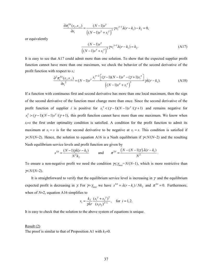
37

( )1

1 22( , ) ( 1) ( ) 0,

( 1)

SAi i i

ii i

s s N s s r k ks N s s

γγ

γ γ

π γ λ−−∂ −= − − =∂ − +

or equivalently

( )1

1 22( 1) ( ) .

( 1)i

i

N s s r k kN s s

γγ

γ γγ λ−− − =

− + (A17)

It is easy to see that A17 could admit more than one solution. To show that the expected supplier profit function cannot have more than one maximum, we check the behavior of the second derivative of the profit function with respect to si:

( )22

12 3

( 1)( 1) ( 1)( , ) ( 1) ( ).( 1)

SAi ii i i

i i

s N s ss s N s r ks N s s

γ γ γγ

γ γ

γ γπ γλ−

−� �− − − +∂ � �= − −

∂ − + (A18)

If a function with continuous first and second derivative has more than one local maximum, then the sign

of the second derivative of the function must change more than once. Since the second derivative of the

profit function of supplier i is positive for ( 1)( 1) /( 1)is N sγ γγ γ< − − + and remains negative for

( 1)( 1) /( 1),is N sγ γγ γ> − − + this profit function cannot have more than one maximum. We know when

si=s the first order optimality condition is satisfied. A condition for the profit function to admit its

maximum at si = s is for the second derivative to be negative at si = s. This condition is satisfied if

γ < N/(N−2). Hence, the solution to equation A16 is a Nash equilibrium if γ < N/(N−2) and the resulting

Nash equilibrium service levels and profit function are given by

12

2

( 1) ( )SA N r ksN kγλ− −= and

( ) 12

( 1) ( )SA N N r kN

γ λπ

− − −= .

To ensure a non-negative profit we need the condition γ < γmax=N/(N−1), which is more restrictive than

γ < N/(N−2).

It is straightforward to verify that the equilibrium service level is increasing in γ and the equilibrium

expected profit is decreasing in γ. For γ = γmax we have 1 2( ) /SAs r k Nkλ= − and 0.SAπ = Furthermore,

when of N=2, equation A16 simplifies to 2

2 1 21

1 2

( ) , for 1,2.( )i

k s ss ir s s

γ γ

γγλ −+= =

It is easy to check that the solution to the above system of equations is unique.

Result (2) The proof is similar to that of Proposition A1 with k2=0.