WP/15/14 Output Gap Uncertainty and Real-Time Monetary Policy Francesco Grigoli, Alexander Herman, Andrew Swiston, and Gabriel Di Bella

Welcome message from author
This document is posted to help you gain knowledge. Please leave a comment to let me know what you think about it! Share it to your friends and learn new things together.
Transcript
WP/15/14
Output Gap Uncertainty and Real-Time
Monetary Policy
Francesco Grigoli, Alexander Herman, Andrew Swiston, and
Gabriel Di Bella

1
© 2015 International Monetary Fund WP/15/14
IMF Working Paper
Western Hemisphere Department
Output Gap Uncertainty and Real-Time Monetary Policy
Prepared by Francesco Grigoli, Alexander Herman, Andrew Swiston, and
Gabriel Di Bella 1
Authorized for distribution by Przemek Gajdeczka
January 2015
Abstract
Output gap estimates are subject to a wide range of uncertainty owing to data revisions and
the difficulty in distinguishing between cycle and trend in real time. This is important given
the central role in monetary policy of assessments of economic activity relative to capacity.
We show that country desks tend to overestimate economic slack, especially during
recessions, and that uncertainty in initial output gap estimates persists several years. Only a
small share of output gap revisions is predictable ex ante based on characteristics like output
dynamics, data quality, and policy frameworks. We also show that for a group of Latin
American inflation targeters the prescriptions from typical monetary policy rules are subject
to large changes due to output gap revisions. These revisions explain a sizable proportion of
the deviation of inflation from target, suggesting this information is not accounted for in real-
time policy decisions.
JEL Classification Numbers: E01, E32, E43, E52
Keywords: Output gap; monetary policy; policy rule; data revisions; real-time; uncertainty;
Brazil; Chile; Colombia; Mexico; Peru; inflation target; business cycle.
Authors’ E-Mail Addresses: [email protected]; [email protected]; [email protected];
1 We would like to thank Tamim Bayoumi, Patrick Blagrave, Alexander Culiuc, Valerie Cerra, Ana Corbacho,
Ernesto Crivelli, Przemek Gajdeczka, Roberto Garcia-Saltos, Huidan Lin, Luca Ricci, Alejandro Werner,
Aleksandra Zdzienicka, and participants of the Western Hemisphere Department Seminars held in August and
September 2014 for helpful comments and suggestions.
This Working Paper should not be reported as representing the views of the IMF.
The views expressed in this Working Paper are those of the author(s) and do not necessarily
represent those of the IMF or IMF policy. Working Papers describe research in progress by the
author(s) and are published to elicit comments and to further debate.

1
Contents Page
Abstract ......................................................................................................................................1
I. Introduction ............................................................................................................................2
II. Output Gap Revisions ...........................................................................................................3 A. Output Gap Definition and Data ...............................................................................3
B. Initial Estimates and Revisions .................................................................................6 C. Robustness Checks ....................................................................................................8
III. Determinants of Output Gap Revisions .............................................................................11 A. Empirical Strategy...................................................................................................11 B. Results .....................................................................................................................13
IV. Policy Implications ............................................................................................................20
A. To Ease, or to Tighten? ...........................................................................................20 B. Setting Monetary Policy in Real Time ....................................................................21
C. Monetary Reaction Functions .................................................................................25 D. Output Gap Revisions and Policy Revisions ..........................................................26 E. Output Gap Revisions and Inflation ........................................................................26
V. Summary and Conclusions..................................................................................................29
Appendix I. Data ......................................................................................................................31
Tables
1. Sources of Revisions to Output Gap Estimates .....................................................................4 2. HP Filter Smoothing Parameter .............................................................................................5
3. Output Gap: Initial Estimates and Revisions .........................................................................6 4. Determinants of the Absolute Revisions of the Output Gap, Baseline ................................14
5. Determinants of the Absolute Revisions of the Output Gap, Extensions ............................17
6. Determinants of the Probability of the Output Gap Changing Sign ....................................19
7. Output Gaps and Revisions ..................................................................................................25
8. Output Gap as a Predictor of Inflation .................................................................................28
Figures
1. Output Gap Revisions by Vintage .........................................................................................7
2. Initial and Final Output Gap Estimates ..................................................................................7 3. Revision Properties ................................................................................................................8 4. Comparison Across Sources ..................................................................................................9 5. Comparison Across US Output Gap Estimates ...................................................................10 6. Real-Time Output Gap Estimates and Confidence Intervals ...............................................21
7. Quarterly Output Gap estimates for LA-5 Economies ........................................................24 8. Policy Deviations Owing to Output Gap Revisions ............................................................27
References ................................................................................................................................33

2
“What is it that no one can see, hear, smell, taste or touch, yet everyone knows is
there? Answer: the output gap." Caroline Baum, Bloomberg, April 12, 2010
I. INTRODUCTION
Reliable output gap measures are essential for policymaking. Both fiscal and monetary policy
reaction functions use output gap estimates as an input in assessing the appropriate settings
for relevant instruments (e.g., the structural fiscal balance or the interest rate). While fiscal
and monetary authorities analyze a wide variety of indicators in assessing the cyclical
position of the economy (including deviations of unemployment from its natural rate), they
frequently resort to the output gap to summarize their assessment of economy-wide spare
capacity.
Despite being widely used in policymaking, initial output gap estimates are characterized by
large uncertainty. This has been extensively documented in the literature. For instance,
Orphanides and van Norden (2002) show how real-time estimates of the U.S. output gap
have often proven highly inaccurate. Ley and Misch (2013) highlight this phenomenon
across a broad range of countries. In a somewhat related fashion, Ho and Mauro (2014) find
that long-term growth forecasts suffer from “optimism bias”, in particular for countries
whose recent growth has been below trend. Uncertainty as to the position of the economy in
the cycle was particularly important at the time of the global financial crisis. For instance the
size of the output gap in the United States has been repeatedly reassessed after 2007, given
the large uncertainty on the impact of the financial crisis on potential output (IMF, 2010).
Needless to say, this uncertainty has important policy implications and can lead to difficulties
in setting a policy that is appropriate given the true state of the economy. This topic has
become particularly important for emerging markets, including many in Latin America. This
is the case as, during the last decade, many of these countries have transitioned toward rule-
based monetary policy frameworks.
This paper revisits the issue of output gap uncertainty by analyzing properties and
determinants of real-time output gap estimates from different sources for the period 1990-
2014. It focuses on the changes in output gap estimates that arise due to ex-post GDP data
revisions and changes in the decomposition of actual GDP data into its cyclical and trend
components. It empirically assesses whether real-time data can predict how much the output
gap will be revised later. The paper then analyzes the implications of output gap uncertainty
for five Latin American economies that have implemented inflation targeting over the last
decade. Our results suggest that country desks tend to overstate economic slack. In addition,
we show that revisions are substantial (especially during recessions), persistent, and, to a
large extent, unpredictable. Finally, we find that revisions help to explain deviations of
inflation from the target, suggesting that this information is not accounted for in real-time
policy decisions.

3
The paper is organized as follows. Section II examines the statistical properties of output gap
estimates and their revisions in order to quantify the uncertainty that surrounds initial
estimates of the output gap. Section III looks at whether these revisions can be predicted
based either on country-specific characteristics or the country’s position in the business cycle
at the time of the initial estimate. Section IV illustrates the policy implications of output gap
uncertainty on five Latin American economies that have operated with inflation targeting
schemes during the last decade. Section V concludes.
II. OUTPUT GAP REVISIONS
This section examines the statistical properties of output gap estimates and their revisions, in
order to evaluate the degree of confidence that can be attached to initial assessments of an
economy’s cyclical position.
A. Output Gap Definition and Data
The output gap is an unobserved, estimated concept, and therefore not known with certainty.
It is defined as the deviation of actual from potential output, as a percent of potential. In
equation (1) below, denotes actual output (measured by real GDP) and represents
potential output, which is defined as the output an economy could produce if all factors of
production were operating at their full employment rates of capacity. The output gap is
denoted by :
(1)
A negative (positive) sign for the output gap indicates that output is below (above) potential.
Estimates of potential output are heavily influenced by the average level of an economy’s
production over time. Revisions to the initial estimate of the output gap could occur as
subsequent developments change estimates of the economy’s productive capacity in previous
periods.
Table 1 shows the possible sources of deviations of initial estimates of the output gap
compared to their final estimates. Let denote the period under analysis. Estimates made
before or during year are forecasts. The first estimate in which data for year is known is
called the initial estimate, and subsequent estimates until the final estimate are called revised
estimates.2 Evaluating revisions to initial estimates requires a decision on which subsequent
vintage will serve as the final estimate. This paper uses as the final estimate the estimated
output gap seven years after the period in question, as revisions typically level off within
seven years. This picks up revisions to the output gap at business cycle frequencies.
2 An annual frequency is assumed but the principles translate to any frequency.

4
As shown in Table 1, deviations between the forecast and final estimate of the output gap can
come from four possible sources. The first is that the forecast serves as an input into the
policymaker’s reaction function. If policymakers base their decisions in part on the forecast
and policy affects output within the year, it is to be expected that the outturn will differ from
the forecast. A second source of uncertainty is forecast error; factors other than policy could
cause the realized output gap to differ from the forecast, and even if policy is implemented as
projected, its effects could differ from what was forecast.
Table 1. Sources of Revisions to Output Gap Estimates
Vintage of estimate Descriptor Possible sources of deviations from final
Forecast Policy reactions, forecast error, data revisions,
uncertainty over potential output
Initial
estimate
Data revisions, uncertainty over potential output
Revised
estimates
Data revisions, uncertainty over potential output
Final
estimate
None, by definition
This paper focuses on the third and fourth sources—revisions to the output gap arising from
data revisions and those arising from changing the decomposition of actual data into its
cyclical and trend components. These sources are present in forecasts and in all ex-post
estimates until the final estimate, as data are revised and estimates of potential output take
into account both data revisions for period and developments in subsequent periods.
This study will be restricted entirely to ex-post estimates—those made after data for the
period under study has been released—in order to isolate the impact of data revisions and
potential output uncertainty and ensure that deviations related to policy reactions and forecast
error do not affect the findings. Modeling the real-time impact of policy reactions and
deviations arising from forecast errors are outside the scope of the analysis.
This paper uses data and forecasts from the International Monetary Fund’s (IMF) World
Economic Outlook (WEO), released twice a year (in the spring and the fall). The WEO
database consists of macroeconomic data and forecasts submitted by country teams and
vetted by the IMF’s Research Department for both internal and multilateral consistency.
Given the importance of working only with ex-post estimates, the vintage from which to
draw the data is critical. The spring WEO was released in May up through 2001 and in April
thereafter; the fall version is typically released in October, and occasionally in September.
Given the production lags, forecasts for the spring publication are performed during February
or March. Given this timeline, in the spring WEO real GDP data for the previous year will

5
continue to be an estimate or forecast for some countries. For this reason, the analysis is
performed with the fall vintages.
Data are available since 1991. Given that the final estimate of the output gap is that measured
seven years after the period in question, the available WEO vintages allow the calculation of
initial estimates and subsequent revisions up to the final estimate from 1990 to 2007. The
WEO database contains real-time estimates of the output gap made by country desks for
many advanced economies throughout this period. Estimates for many other economies,
however, begin only in 2008. There is no prescribed estimation methodology, but the
estimates are used by the IMF in discussions with country authorities over appropriate
economic policies, underscoring the importance of an accurate assessment.
In order to cover as many countries as possible, we estimate output gaps using potential GDP
obtained by applying the Hodrick-Prescott (HP) filter on real GDP data from the WEO and
compare with the estimates from country desks where available. As shown in Table 2, we
formally test which size of the smoothing parameter commonly used for annual data (100
and 6.25) better fits the estimates provided in the WEO and in the OECD’s Economic
Outlook databases by regressing both filtered series on the WEO and OECD data.3 Table 3
reports the root mean squared errors (RMSE) and R-squared values below, suggesting that
set to 100 is a better analog of both WEO and OECD data. This suggests that country desks
tend to interpret changes in real GDP as changes in cycle rather than in trend. Thus, in the
analysis that follows we use HP-filtered data with set to 100 for all countries while
performing robustness checks on the results using the desk-provided estimates and HP-
filtered data with set to 6.25.4 The baseline dataset has an average sample size of 176
countries per year, for a total of 3,018 observations.
Table 2. HP Filter Smoothing Parameter
3 As noted in Baxter and King (1995), setting to 10 or below closely replicates the statistical properties of the
Baxter-King filter.
4 We run the HP filter over all available historical data plus the forecast available in the WEO database to
mitigate endpoint problems.
(λ=100) (λ=6.25) (λ=100) (λ=6.25)
Observed WEO data 2.11 2.25 0.47 0.40
Observed OECD data 1.10 1.47 0.72 0.51
Source: Authors' calculations.
RMSE R-squared
HP filtered WEO data HP filtered WEO data

6
B. Initial Estimates and Revisions
Initial assessments of an economy’s cyclical position are subject to a high degree of
uncertainty. Table 3 shows that revisions to the output gap are of the same order of
magnitude as the initial estimates of the output gap itself, and that about one-third of
economies have an output gap that changes signs between the initial and final estimates.
Countries are divided into three groups to evaluate whether there are differences across types
of country. Advanced economies include all OECD members as of 1990 (the beginning of
the sample). Low-income economies include any country with a GNI per capita of $1,045 or
less in 2012. Emerging economies are all those that are not included in the other two groups.5
Revisions for emerging and low-income economies are larger than those for advanced
economies and the estimates are more likely to switch signs. All these features of the data
confirm the findings of Ley and Misch (2013).
Table 3. Output Gap: Initial Estimates and Revisions (Percent of potential GDP)
Uncertainty over the output gap persists for several years after the period under analysis.
Figure 1 shows the absolute value of marginal output gap revisions in each vintage and at
various percentiles. In the year following the initial estimate, the output gap of the typical
country is revised by 0.9 percentage points. Two years later, the absolute value of the median
revision remains nearly half a percentage point. Seven years after the year under analysis, a
quarter of all countries experience revisions of half a percentage point and ten percent of all
countries experience an output gap revision of a full percentage point.
In addition, initial assessments of the cyclical position overestimate the amount of slack in
the economy. Actual output is 1.0 percent below potential output in initial estimates, but only
0.2 percent below potential in final estimates, and median revisions to the output gap exceed
0.5 percent of potential for all types of countries (Table 1; Figure 2, left panel). We call this
phenomenon “excess capacity bias.”
5 See Appendix I for a complete list of countries in each group.
Number Percent
of Median Standard Median Standard Median Standard switching
countries deviation deviation deviation signs
All countries 176 -0.97 5.12 -0.22 5.57 0.75 3.89 32.3
Advanced 24 -0.24 1.61 0.27 2.49 0.51 1.67 22.9
Emerging 122 -0.98 5.47 -0.34 5.90 0.64 4.11 32.7
Low-income 30 -1.77 5.28 -0.22 5.93 1.55 4.16 38.8
Source: Authors' calculations.
Initial estimate Final estimate Revision

7
Figure 1. Marginal Output Gap Revisions by Vintage (Absolute value; percent of potential GDP)
Two factors interact to produce excess capacity bias. First, initial estimates of economic
activity tended to be revised upward in later vintages (Figure 2, middle panel). This fact by
itself would not lead to a bias towards excess capacity, as persistent upward data revisions
would tend to raise both actual and potential output without a substantial impact on the
estimated cyclical position. However, economic activity tended to underperform IMF
forecasts, in line with the findings of Ho and Mauro (2014) and Timmermann (2007). This
second factor worked to keep cumulative revisions to estimated potential growth roughly
neutral, at less than 0.1 percent of potential output, on average (Figure 2, right panel). The
combination of upward revisions to past activity and downward revisions to current activity
(relative to the forecast) results in the lower level of excess capacity in final estimates
compared to initial estimates.
Figure 2. Initial and Final Output Gap Estimates
0.0
0.5
1.0
1.5
2.0
2.5
3.0
3.5
4.0
t+2 t+3 t+4 t+5 t+6 t+7
Median 75th percentile 90th percentile
Source: Authors' calculations.
Source: Authors' calculations.
-2.0
-1.5
-1.0
-0.5
0.0
0.5
1.0
All c
ou
ntr
ies
Ad
vance
d
Em
erg
ing
Low
-inco
me
Initial Final
Output gap
(percent of potential)
2.0
2.5
3.0
3.5
4.0
4.5
5.0
All c
ou
ntr
ies
Ad
vance
d
Em
erg
ing
Low
-inco
me
Initial Final
Potential GDP growth
(percent)
2.0
2.5
3.0
3.5
4.0
4.5
5.0
All c
ou
ntr
ies
Ad
vance
d
Em
erg
ing
Low
-inco
me
Initial Final
Real GDP growth
(percent)
8
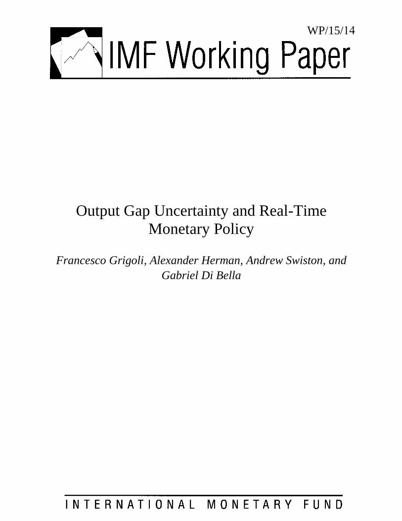
Initial assessments of an economy’s cyclical position are least reliable during recessions.
Figure 3 compares the full sample and a subsample restricted to episodes in which the initial
estimate of real GDP growth was negative, displaying for each group of observations the
average absolute revision and the standard deviation of revisions.6 It shows that absolute
revisions to the output gap, actual growth, and potential growth are 30 to 50 percent larger
during downturns than in normal times, and the wider distribution of revisions—30 percent
higher than in the full sample—highlights the additional uncertainty over the cyclical
position of an economy when growth is negative.
Figure 3. Revision Properties (Cumulative revisions, final estimate minus initial estimate)
C. Robustness Checks
The key features of initial assessments of an economy’s cyclical position and its subsequent
revisions are 1) a high degree of uncertainty that persists several years beyond the period
under analysis; 2) initial estimates have an excess capacity bias, overestimating the amount
of spare capacity in an economy; and 3) increased uncertainty around cyclical turning points,
in particular during economic downturns.
In order to ensure that these features of the data are not unique to the WEO dataset or our use
of the HP filter to estimate potential output and the output gap, we perform several
robustness checks.
6 Clearly, turning points marking an acceleration of an economy could also be analyzed. Given that potential
growth rates differ across economies, negative real GDP growth (especially at the annual frequency) may not
catch all cyclical turning points, but it is probable that most observations in this subsample are turning points
(with the most likely exception being economies in an extended period of negative growth). The results hold
when negative growth is defined using the final estimate rather than the initial estimate.
Source: Authors' calculations.
0
1
2
3
4
5
6
All years Years with
negative
growth
All years Years with
negative
growth
Average absolute
revision
Standard deviation
of revisions
Output gap
0
1
2
3
4
5
6
All years Years with
negative
growth
All years Years with
negative
growth
Average absolute
revision
Standard deviation
of revisions
Real GDP growth
0
1
2
3
4
5
6
All years Years with
negative
growth
All years Years with
negative
growth
Average absolute
revision
Standard deviation
of revisions
Potential GDP growth
9
First, we use HP-filtered data generated by setting equal to 6.25.7 The median revisions are
much lower than those when is set to 100, suggesting that the excess capacity bias depends
on the parameter , and therefore on the extent to which real growth fluctuations are
interpreted as structural. However, the ratios of standard deviations to medians are
dramatically larger. This suggests that using set to 6.25 creates higher levels of normalized
volatility in output gap measurements and more evenly dispersed revisions across zero,
implying an even higher uncertainty about the direction of the revision.
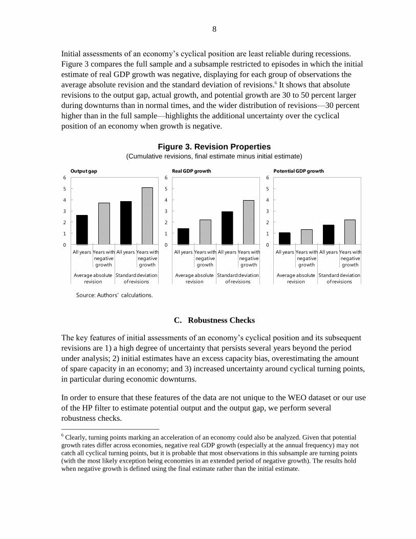
Second, we use estimates of the output gap from two cross-country sources: the OECD’s
Economic Outlook database and the WEO database. The December edition of the Economic
Outlook was used, as its release coincides most closely with the Fall WEO. As with the WEO
estimates, the OECD estimates are submitted directly by country teams using their own
judgment as to the amount of spare capacity in each economy. Using estimates that rely on
the judgment of analysts covering the economies in question should reveal whether the use of
the HP filter is driving the results.
Both the WEO and OECD data cover mostly advanced economies, so Figure 4 compares the
key metrics presented above with the HP-filtered estimates, all using the same sample of
advanced economies (see Appendix I). Country desks’ estimates display at least as much
persistent uncertainty in revisions and excess capacity bias as the HP-filtered estimates. In
fact, the right panel in Figure 4 shows that the typical revisions from these sources are larger
and more variable than those from the HP-filtered data.
Figure 4. Comparison Across Sources (Data for advanced economies)
7 See Ravn and Uhlig (2002).
Source: Authors' calculations.
-0.5
-0.4
-0.3
-0.2
-0.1
0.0
0.1
0.2
0.3
0.4
0.5
HP-filtered OECD WEO
Initial Final
Output gap estimates
(percent of potential
output)
0.0
0.5
1.0
1.5
2.0
2.5
Average absolute
revision
Standard deviation
of revisions
HP-filtered
OECD
WEO
Output gap revisions
(cumulative revision)
0.0
0.1
0.2
0.3
0.4
0.5
0.6
0.7
0.8
t+2 t+3 t+4 t+5 t+6 t+7
HP-filtered
OECD
WEO
Output gap revisions by vintage
(average absolute value of
marginal revision)
10
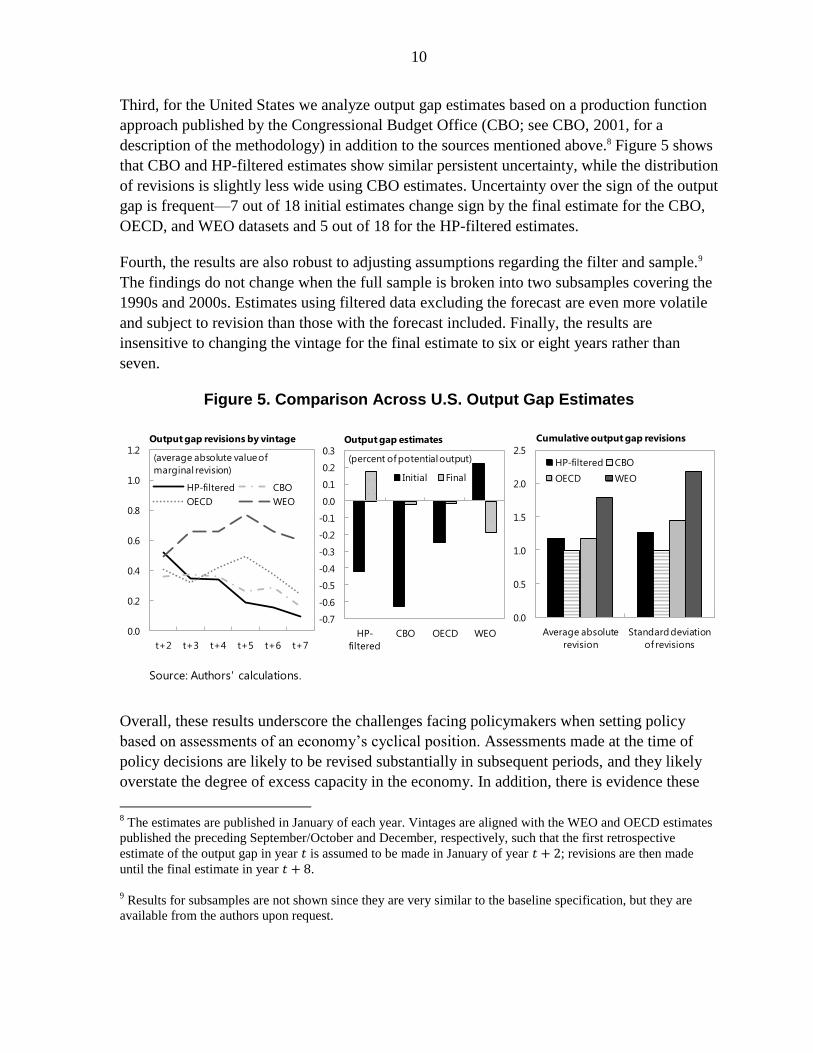
Third, for the United States we analyze output gap estimates based on a production function
approach published by the Congressional Budget Office (CBO; see CBO, 2001, for a
description of the methodology) in addition to the sources mentioned above.8 Figure 5 shows
that CBO and HP-filtered estimates show similar persistent uncertainty, while the distribution
of revisions is slightly less wide using CBO estimates. Uncertainty over the sign of the output
gap is frequent—7 out of 18 initial estimates change sign by the final estimate for the CBO,
OECD, and WEO datasets and 5 out of 18 for the HP-filtered estimates.
Fourth, the results are also robust to adjusting assumptions regarding the filter and sample.9
The findings do not change when the full sample is broken into two subsamples covering the
1990s and 2000s. Estimates using filtered data excluding the forecast are even more volatile
and subject to revision than those with the forecast included. Finally, the results are
insensitive to changing the vintage for the final estimate to six or eight years rather than
seven.
Figure 5. Comparison Across U.S. Output Gap Estimates
Overall, these results underscore the challenges facing policymakers when setting policy
based on assessments of an economy’s cyclical position. Assessments made at the time of
policy decisions are likely to be revised substantially in subsequent periods, and they likely
overstate the degree of excess capacity in the economy. In addition, there is evidence these
8 The estimates are published in January of each year. Vintages are aligned with the WEO and OECD estimates
published the preceding September/October and December, respectively, such that the first retrospective
estimate of the output gap in year is assumed to be made in January of year ; revisions are then made
until the final estimate in year .
9 Results for subsamples are not shown since they are very similar to the baseline specification, but they are
available from the authors upon request.
Source: Authors' calculations.
-0.7
-0.6
-0.5
-0.4
-0.3
-0.2
-0.1
0.0
0.1
0.2
0.3
HP-
filtered
CBO OECD WEO
Initial Final
Output gap estimates
(percent of potential output)
0.0
0.5
1.0
1.5
2.0
2.5
Average absolute
revision
Standard deviation
of revisions
HP-filtered CBO
OECD WEO
Cumulative output gap revisions
0.0
0.2
0.4
0.6
0.8
1.0
1.2
t+2 t+3 t+4 t+5 t+6 t+7
HP-filtered CBO
OECD WEO
Output gap revisions by vintage
(average absolute value of
marginal revision)

11
problems are more acute during turning points, as revisions tend to be larger during
recessions.
III. DETERMINANTS OF OUTPUT GAP REVISIONS
The previous section establishes the wide range of uncertainty that surrounds initial estimates
of the output gap. This section looks at whether output gap revisions can be predicted based
on either country-specific characteristics or the country’s position in the business cycle at the
time of the initial estimate. Although we find several significant determinants of output gap
revisions, a large share of revisions remains unexplained, suggesting that they may not be
predictable at the time policy decisions are made.
A. Empirical Strategy
Some variables may explain the direction of subsequent output gap revisions, while others
may only be informative about the magnitude of revisions. In order to maximize the
explanatory power of the information at our disposal at the time of initial estimates, we
attempt to explain the size of output gap revisions rather than the direction in which the
revisions occur.10 Let denote the absolute value of the cumulative output
gap revision for country at time . This can be modeled as:
(2)
Where is the intercept, is a matrix of variables including the a set of covariates for
country at time and measured at time , is a matrix including other time-invariant
covariates measured at the most recent point in time, and are the coefficients on these
matrices, and is a mean zero error term that captures unexplained heterogeneity.
Equation (2) is estimated using ordinary least squares (OLS) applied to a pooled panel
sample of annual observations, correcting the standard errors for heteroskedasticity and
autocorrelation. As a robustness check, we also estimate equation (2) with a further
correction of the standard errors for cross-sectional dependence.
The selection of the control variables and included in the specifications relies on
our understanding, guided by previous empirical research (see, in particular, Ley and Misch,
2014), of what factors may determine the magnitude of the output gap revisions.
10
Note that the revisions of output gap estimates made ex ante would be even less predictable. See Appendix I
for a detailed description of the variables.

12
In order to maximize the usefulness of the findings to policy decisions, we also investigate
the determinants of output gap revisions that are large enough to change the sign of the gap,
since real-time assessments of whether the economy is above or below potential output play a
key role in policy decisions. To investigate the determinants of changes in the sign of the
output gap, we estimate the following population-averaged panel probit model11 on the same
regressors as in the baseline specification:
(3)
where is the probability function, and is a binary variable taking the value one
when the sign of the output gap of country at time measured at time is the opposite
of the sign of the same output gap measured at time . To avoid mild fluctuations around
potential GDP, we consider only episodes in which the output gap revision is larger than half
a percentage point of potential GDP. Our estimations perform a correction for
heteroskedasticity and autocorrelation of the standard errors.12
We group the baseline regressors into four categories. A first category includes variables
related to domestic or world GDP dynamics. In particular, we control for the size of the
output gap measured at . A very large positive or negative output gap may signal a
change in trend growth that is incorporated only gradually into estimates of potential output
and thus we expect a positive impact on the size of revisions. Also, we include domestic and
world real GDP growth surprises in time (measured at time to have actual figures),
which are defined as the deviation of domestic (or world) real GDP growth from its mean
within the last 10 years. Thus, when a surprise in growth occurs, either domestic or
worldwide, it increases the difficulty of decomposing actual output data into its trend and
cyclical components, negatively affecting the ability to estimate the output gap and
increasing the expected size of its revisions.
A second category of variables attempts to gauge macroeconomic uncertainty. To this end,
we use the standard deviation of domestic real GDP growth over the last 10 years measured
11
The alternative is to use logit regressions, assuming an error term that is logistically distributed. As a
robustness check, we perform logit regressions that are not shown because they return similar results. Results
are available from the authors upon request.
12 The estimated coefficients of a probit model do not quantify the influence of the covariates on the probability
of a sign change of the output gap because they are parameters of the latent model. As such, they only measure
the effect of a regressor on the latent propensity for a positive result. The effect of a unit change of a covariate
on the dependent variable when the other covariates are constant is represented by the marginal effect. This can
then be interpreted similarly to the linear regression coefficient, which directly measures the marginal effect of
an explanatory variable on the dependent one. Hence, for the probit estimations we only report the
corresponding marginal effects.

13
at , as a proxy of historical volatility in the economy. We also include the share of
natural resource rents (or economic profits) in GDP to proxy natural resource price
movements that are not necessarily reflected in inflation, as well as volume changes. In a
broader sense, this variable is a proxy for structural changes in the economy.13 It is
constructed as the sum of oil, natural gas, coal, mineral, and forest rents, which greatly
depend on the corresponding price. Finally, we also include the most commonly used proxy
for macroeconomic uncertainty, which is inflation. All these variables are expected to be
positively associated with the size of revisions.
A third category of variables captures the presence of policy frameworks. In particular, we
include dummy variables for the presence of inflation targeting and fiscal rules that are
specified in terms of some fiscal aggregate adjusted for the cycle (here we call them cyclical
fiscal rules). These frameworks should activate countercyclical policies which should help
keep output relatively near its trend level, reducing the size of revisions. Fiscal rules,
however, are often introduced when fiscal discipline is weak and their adoption can be
accompanied by significant adjustments when conditions for triggering escape clauses are
not met. Thus, the expected effect on output gap revisions is ambiguous.
A last category of variables is supposed to capture the degree of statistical capacity common
to different groups of countries. Advanced economies are likely to have good and timely data
and thus revisions to actual data and the output gap are expected to be smaller. In contrast,
data timeliness and availability is more heterogeneous in low-income countries (LICs),
possibly affecting the reliability of initial releases of GDP data and increasing the size of
output gap revisions. This is similar to what happens in a number of small economies (those
with a population below the 10th
percentile of the population distribution). Beyond data
quality, LICs and small economies may be subject to shocks (such as natural disasters)
whose effects are hard to decompose between the trend and the cycle in real time. These
three factors are represented by dummy variables.
B. Results
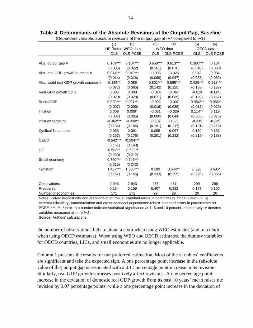
Table 4 presents evidence on the determinants of the cumulative absolute revisions of the
output gap. We run the baseline specification on an unbalanced sample of 2,943 observations
for 171 countries over the period 1990-2007 using the baseline dataset of HP-filtered real
GDP data. For robustness, we estimate the same specification using estimates for the output
gap provided to the WEO by country desks, as well as OECD estimates, and by running an
alternate specification that corrects the standard errors for cross-sectional dependence. As the
WEO output gap estimates cover only 29 countries (26 countries in the case of the OECD),
13
Since there are no vintages available for rents in percent of GDP, we assume that the data are the same as at
time .
14
Table 4. Determinants of the Absolute Revisions of the Output Gap, Baseline (Dependent variable: absolute revisions of the output gap at t+7 compared to t+1)
the number of observations falls to about a sixth when using WEO estimates (and to a tenth
when using OECD estimates). When using WEO and OECD estimates, the dummy variables
for OECD countries, LICs, and small economies are no longer applicable.
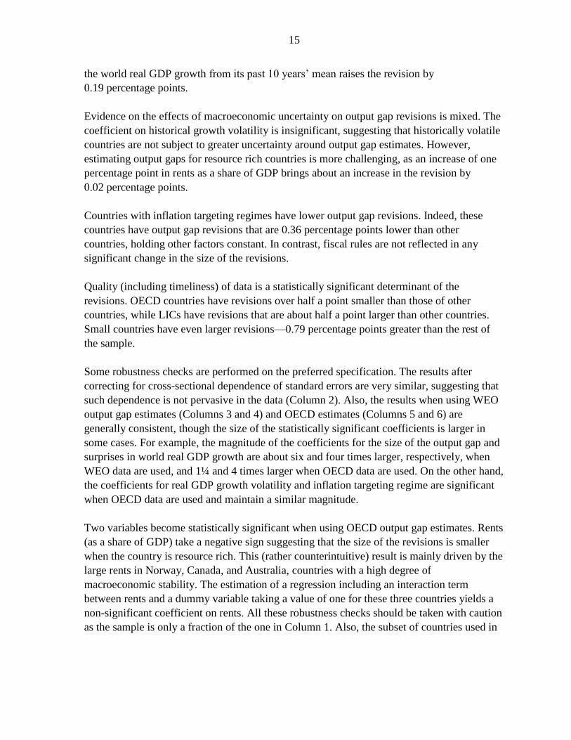
Column 1 presents the results for our preferred estimation. Most of the variables’ coefficients
are significant and take the expected sign. A one percentage point increase in the (absolute
value of the) output gap is associated with a 0.11 percentage point increase in its revision.
Similarly, real GDP growth surprises positively affect revisions. A one percentage point
increase in the deviation of domestic real GDP growth from its past 10 years’ mean raises the
revision by 0.07 percentage points, while a one percentage point increase in the deviation of
(1) (2) (3) (4) (5) (6)
OLS OLS PCSE OLS OLS PCSE OLS OLS PCSE
Abs. output gap # 0.109*** 0.104*** 0.658*** 0.613*** 0.180*** 0.134
(0.035) (0.022) (0.161) (0.070) (0.040) (0.083)
Abs. real GDP growth surprise # 0.074*** 0.049*** -0.035 -0.026 0.043 0.034
(0.014) (0.018) (0.069) (0.057) (0.083) (0.089)
Abs. world real GDP growth surprise # 0.189** 0.085 0.801*** 0.568*** 0.925*** 0.612***
(0.077) (0.065) (0.142) (0.125) (0.188) (0.138)
Real GDP growth SD # 0.005 0.008 -0.014 -0.047 -0.019 -0.005
(0.020) (0.028) (0.071) (0.085) (0.139) (0.152)
Rents/GDP 0.020*** 0.021*** -0.002 -0.007 -0.054*** -0.056**
(0.007) (0.006) (0.016) (0.036) (0.013) (0.023)
Inflation 0.009 0.009* -0.061 -0.039 0.114** 0.119
(0.007) (0.005) (0.060) (0.044) (0.055) (0.075)
Inflation targeting -0.362*** -0.330** -0.107 -0.171 -0.235 -0.225
(0.135) (0.154) (0.191) (0.217) (0.191) (0.218)
Cyclical fiscal rules 0.056 0.091 0.058 0.067 0.130 0.138
(0.167) (0.178) (0.201) (0.232) (0.218) (0.188)
OECD -0.542*** -0.594***
(0.151) (0.140)
LIC 0.503** 0.522**
(0.230) (0.212)
Small economy 0.790*** 0.745***
(0.216) (0.242)
Constant 1.437*** 1.685*** 0.189 0.544** 0.328 0.685*
(0.157) (0.165) (0.333) (0.255) (0.296) (0.366)
Observations 2,943 2,943 437 437 299 299
R-squared 0.164 0.109 0.407 0.382 0.157 0.100
Number of economies 171 171 29 29 26 26
Source: Authors' calculations.
WEO data OECD dataHP filtered WEO data
Notes: Heteroskedasticity and autocorrelation robust standard errors in parentheses for OLS and FGLS;
heteroskedasticity, autocorrelation and cross-sectional dependence robust standard errors in parentheses for
PCSE; ***, **, * next to a number indicate statistical significance at 1, 5 and 10 percent, respectively; # denotes
variables measured at time t+1 .
15
the world real GDP growth from its past 10 years’ mean raises the revision by
0.19 percentage points.
Evidence on the effects of macroeconomic uncertainty on output gap revisions is mixed. The
coefficient on historical growth volatility is insignificant, suggesting that historically volatile
countries are not subject to greater uncertainty around output gap estimates. However,
estimating output gaps for resource rich countries is more challenging, as an increase of one
percentage point in rents as a share of GDP brings about an increase in the revision by
0.02 percentage points.
Countries with inflation targeting regimes have lower output gap revisions. Indeed, these
countries have output gap revisions that are 0.36 percentage points lower than other
countries, holding other factors constant. In contrast, fiscal rules are not reflected in any
significant change in the size of the revisions.
Quality (including timeliness) of data is a statistically significant determinant of the
revisions. OECD countries have revisions over half a point smaller than those of other
countries, while LICs have revisions that are about half a point larger than other countries.
Small countries have even larger revisions—0.79 percentage points greater than the rest of
the sample.
Some robustness checks are performed on the preferred specification. The results after
correcting for cross-sectional dependence of standard errors are very similar, suggesting that
such dependence is not pervasive in the data (Column 2). Also, the results when using WEO
output gap estimates (Columns 3 and 4) and OECD estimates (Columns 5 and 6) are
generally consistent, though the size of the statistically significant coefficients is larger in
some cases. For example, the magnitude of the coefficients for the size of the output gap and
surprises in world real GDP growth are about six and four times larger, respectively, when
WEO data are used, and 1¼ and 4 times larger when OECD data are used. On the other hand,
the coefficients for real GDP growth volatility and inflation targeting regime are significant
when OECD data are used and maintain a similar magnitude.
Two variables become statistically significant when using OECD output gap estimates. Rents
(as a share of GDP) take a negative sign suggesting that the size of the revisions is smaller
when the country is resource rich. This (rather counterintuitive) result is mainly driven by the
large rents in Norway, Canada, and Australia, countries with a high degree of
macroeconomic stability. The estimation of a regression including an interaction term
between rents and a dummy variable taking a value of one for these three countries yields a
non-significant coefficient on rents. All these robustness checks should be taken with caution
as the sample is only a fraction of the one in Column 1. Also, the subset of countries used in
16
Columns 3 to 6 may suffer from selection bias because the countries included are mainly
advanced economies.14
Finally, we run the same specifications in Columns 1 and 2 using HP-filtered WEO data that
are generated by equal to 6.25. The results are very similar to the ones reported in Columns
1 and 2 and suggest that the choice of the smoothing parameter does not affect the main
conclusions.15
The goodness of fit of the different specifications falls in the 10 to 41 percent range. This
suggests that a large component of the revisions behaves as a white noise process, and thus, it
cannot be explained by factors known to policymakers.
We also estimate the baseline specification without dummy variables for country groups.
One may argue these dummies pick up effects other than the ones they are constructed for
and that, as a result, the explanatory power may be even lower than in the baseline
estimation. The results, however, suggest that this is not the case as the continuous variables
present similar coefficients and the R-squared is close to the one of the baseline, so the
results are not shown.
In order to reduce the likelihood of omitted variable bias, in Table 5 we present some
extensions to the baseline specification. The baseline results are generally robust when other
explanatory variables are added. First, we test if adherence to data dissemination standards
defined by the IMF, the General Data Dissemination System (GDDS) or the Special Data
Dissemination Standard (SDDS)16, affect the size of the revisions. While we expect a
negative effect, the results are insignificant (Column 1).
Social or political conflicts can be detrimental to output gap estimation because of the
destruction of human and physical capital (including assessing the impact on the economy’s
productive capacity). To capture this, we include a dummy variable taking a value of one if
the loss of life due to conflict is considerable, and expect it to be positively associated with
the size of the revisions. We find the coefficient on this dummy to be statistically
insignificant (Column 2).
14
We also run a specification including a dummy taking value one during the 1990s to explore whether there
was a change over time in the size of the revisions. However, the coefficient is not statistically significant.
15 Results are available from the authors upon request.
16 The difference between the two standards is the level of data requirements, with the SDDS being more
demanding.

17
Table 5. Determinants of the Absolute Revisions of the Output Gap,
Extensions (Dependent variable: absolute revisions of the output gap at t+7 compared to t+1; HP filtered data)
(1) (2) (3) (4) (5)
Abs. output gap # 0.109*** 0.109*** 0.108** 0.107** 0.051
(0.035) (0.036) (0.047) (0.046) (0.045)
Abs. real GDP growth surprise # 0.074*** 0.074*** 0.081*** 0.081*** 0.065***
(0.014) (0.014) (0.014) (0.014) (0.013)
Abs. world real GDP growth surprise # 0.200** 0.189** 0.164* 0.166* 0.214***
(0.077) (0.077) (0.087) (0.087) (0.076)
Real GDP growth SD # 0.003 0.005 0.029 0.031 -0.023
(0.020) (0.020) (0.027) (0.028) (0.020)
Rents/GDP 0.021*** 0.020*** 0.017** 0.017** 0.015**
(0.007) (0.007) (0.008) (0.008) (0.007)
Inflation 0.009 0.010 0.010 0.011* 0.011
(0.007) (0.007) (0.007) (0.006) (0.007)
Inflation targeting -0.394*** -0.361*** -0.274* -0.304** -0.344***
(0.150) (0.134) (0.140) (0.136) (0.126)
Cyclical fiscal rules 0.048 0.053 0.090 0.115 0.071
(0.172) (0.167) (0.164) (0.166) (0.148)
OECD -0.578*** -0.544*** -0.328* -0.316* -0.549***
(0.156) (0.150) (0.181) (0.182) (0.139)
LIC 0.542** 0.506** 0.482* 0.538** 0.582**
(0.238) (0.230) (0.274) (0.268) (0.234)
Small economy 0.828*** 0.786*** 0.722***
(0.219) (0.216) (0.204)
GDDS -0.254
(0.214)
SDDS 0.036
(0.155)
Conflict -0.166
(0.291)
Bureaucratic quality -0.086
(0.081)
Control of corruption -0.074
(0.059)
Abs. average future real GDP growth differential 0.123***
(0.036)
Constant 1.458*** 1.441*** 1.484*** 1.494*** 1.327***
(0.170) (0.156) (0.251) (0.218) (0.156)
Observations 2,943 2,943 2,241 2,241 2,942
R-squared 0.165 0.164 0.183 0.183 0.185
Number of economies 171 171 129 129 171
Notes: All estimations are performed with pooled OLS; heteroskedasticity and autocorrelation robust
standard errors in parentheses; ***, **, * next to a number indicate statistical significance at 1, 5 and 10
percent, respectively; # denotes variables measured at time t+1 .
Source: Authors' calculations.

18
Also, we control for institutional quality. Corruption or low bureaucratic quality may
negatively affect data quality and data production processes. For example, if institutional
quality is weak, there may be scope for data manipulation with the aim of obtaining political
advantage. Hence, we expect the coefficients on both variables to be negative. The estimation
yields statistically insignificant coefficients (Columns 3 and 4).
Finally, we introduce information about future GDP growth. In principle, a sharp
acceleration or slowdown in growth after year should play a role in revisions to the
estimated output gap in by changing the decomposition of actual data into trend and cycle.
We measure the change in future growth by taking the absolute value of the difference in
average GDP growth between the five years following and the five years preceding it. The
coefficient on this variable is significant and indicates that an absolute change of one
percentage point in future growth increases the size of the output gap revision by 0.12
percentage points. The incorporation of this variable turns the coefficient on the (absolute)
size of the output gap insignificant, suggesting some redundancy between the two. Moreover,
the increase in explanatory power is modest (Column 5).17
Similar to the robustness check for the baseline specification, we exclude the dummy
variables for country groups and re-estimate Columns 1 to 5. While the coefficients for the
continuous variables show similar magnitudes, bureaucratic quality, and control of corruption
turn significant with the expected negative sign, suggesting a fairly high degree of correlation
with the excluded dummies (results not shown).
Table 6 shows the marginal effects derived from the probit estimations on the baseline
dataset of HP-filtered WEO data. Column 1 presents the results using the same baseline
specification as in Table 4. A one percentage point increase in the size of the output gap
reduces the probability of a change in the sign of the output gap by 0.07 percent. This result
(along with the findings of a positive association between an increase in the size of the output
gap and the size of the revisions) suggests that countries that are far away from the potential
output are unlikely to have revisions large enough to change the sign of the output gap. Also,
real GDP growth surprises increase the probability of the output gap changing sign, but to a
smaller extent.
Macroeconomic uncertainty affects the probability of a sign change in the output gap during
the revision period, but the size of the coefficient is relatively small. An increase in inflation
by one percentage point increases such probability by 0.002 percent. Being an inflation
targeter reduces the probability of a sign change by 0.09 percent. Interestingly, countries with
17
As in Ley and Misch (2013), we test if countries with an IMF program have higher output gap revisions (see
Dreher et al., 2008), and the coefficient is insignificant.

19
cyclical fiscal rules are more likely to observe changes in the sign of the output gap during
the revision period by 0.12 percent.
Table 6. Determinants of the Probability of the Output Gap Changing Sign (Dependent variable: binary variable, 1 if output gap changes sign at t+7; HP filtered data; marginal
effects)
Statistical capacity matters. Consistent with the results of Tables 4 and 5, being an OECD
country reduces the probability of a sign change in the output gap by 0.14 percent, while
being a LIC increases it by 0.11 percent.
(1) (2) (3) (4) (5) (6)
Abs. output gap # -0.071*** -0.071*** -0.071*** -0.087*** -0.086*** -0.065***
(0.007) (0.007) (0.007) (0.007) (0.007) (0.007)
Abs. real GDP growth surprise # 0.005* 0.005* 0.005* 0.003 0.003 0.008***
(0.003) (0.003) (0.002) (0.002) (0.002) (0.002)
Abs. world real GDP growth surprise # 0.009 0.012 0.009 0.001 0.003 0.006
(0.014) (0.014) (0.014) (0.016) (0.016) (0.014)
Real GDP growth SD # 0.000 -0.000 0.000 0.006 0.006* 0.002
(0.004) (0.004) (0.004) (0.003) (0.003) (0.004)
Rents/GDP -0.000 -0.000 -0.000 -0.001 -0.001 0.000
(0.001) (0.001) (0.001) (0.001) (0.001) (0.001)
Inflation 0.002** 0.002* 0.002** 0.002** 0.002** 0.002**
(0.001) (0.001) (0.001) (0.001) (0.001) (0.001)
Inflation targeting -0.085*** -0.055** -0.085*** -0.077*** -0.081*** -0.085***
(0.026) (0.028) (0.026) (0.025) (0.025) (0.025)
Cyclical fiscal rules 0.116* 0.143** 0.116* 0.112* 0.102 0.114*
(0.068) (0.068) (0.068) (0.068) (0.068) (0.067)
OECD -0.135*** -0.131*** -0.135*** -0.102*** -0.141*** -0.133***
(0.029) (0.029) (0.029) (0.035) (0.031) (0.029)
LIC 0.106*** 0.100*** 0.106*** 0.100** 0.130*** 0.096***
(0.037) (0.037) (0.036) (0.051) (0.049) (0.037)
Small economy 0.050 0.039 0.050 0.065
(0.041) (0.042) (0.041) (0.042)
GDDS -0.039
(0.029)
SDDS -0.071***
(0.026)
Conflict -0.021
(0.053)
Bureaucratic quality -0.022
(0.015)
Control of corruption 0.010
(0.011)
Abs. average future real GDP growth differential -0.019***
(0.005)
Observations 2,943 2,943 2,943 2,241 2,241 2,942
Number of economies 171 171 171 129 129 171
Notes: All estimations are performed with pooled Probit OLS. Heteroskedasticity and autocorrelation robust
standard errors in parentheses; ***, **, * next to a number indicate statistical significance at 1, 5 and 10 percent,
respectively; # denotes variables measured at time t+1 .
Source: Authors' calculations.
20
Columns 2 to 6 report the results of extensions to the baseline specification. The baseline
regressors are robust, with the exception of real GDP growth surprises which loses
significance when the institutional quality variables are included and the dummy for small
economies is dropped. Among the additional regressors, SDDS (but not GDDS) is significant
and takes the expected negative sign. A shift in future GDP growth relative to past GDP
growth reduces the probability of the output gap switching sign. These results are robust to
the exclusion of country group dummies from the specification.
Overall, these regressions predict a low share of the variation in output gap revisions. Given
that they make use of some information that is not known until after the period under
analysis, it is reasonable to expect that the predictability of output gap revisions ex ante,
when it would be useful for policy decisions, is even lower.
IV. POLICY IMPLICATIONS
This paper has illustrated the wide range of uncertainty that typically characterizes
assessments of the cyclical position of economies around the world. It has also shown that
only a small share of this uncertainty is likely to be explained by factors known to
policymakers in real time. This section illustrates some policy implications of these findings,
focusing on five Latin American economies (LA-5) that have implemented active
countercyclical monetary policies over the last decade.
A. To Ease, or to Tighten?
The historical output gap data and revisions described above can be used to construct a
confidence interval around any initial or revised estimate of the output gap. The width of the
confidence interval will vary by country, depending on the historical distribution of its output
gap revisions. It will also vary by the vintage of revision, with a wider confidence interval for
an initial estimate than for a revised estimate that is closer in time to the final estimate.
Figure 6 shows initial estimates of the output gap for Brazil, Chile, Colombia, Mexico, and
Peru for 2008-13. Figure 6 also shows confidence intervals calculated using the distribution
of cumulative revisions to initial estimates over 1990-2007. The magnitude of the confidence
intervals encompasses a wide range of potential outcomes. Only in rare cases is there a high
degree of certainty about whether policy should be contractionary, neutral, or expansionary;
for most countries in most years, there is a non-negligible probability that the appropriate
policy could be in any of those three categories.

21
Figure 6. Real-Time Output Gap Estimates and Confidence Intervals (Output gap in percent of potential GDP)
B. Setting Monetary Policy in Real Time
The confidence intervals provide a broad view of how uncertain the cyclical position of any
economy is, but are based on annual observations, so are less applicable for monetary policy
decisions that make use of higher-frequency data. In this section, we construct real-time
quarterly output gap estimates and use them to estimate monetary policy reaction functions
based on real-time data.
Sources: IMF, World Economic Outlook database; and authors' calculations.
-8
-6
-4
-2
0
2
4
6
8
2008 2009 2010 2011 2012 2013
Brazil
Output gap (percent) +/- 1 Standard deviation +/- 2 Standard deviations
-10
-8
-6
-4
-2
0
2
4
6
8
2008 2009 2010 2011 2012 2013
Chile
-6
-4
-2
0
2
4
6
8
2008 2009 2010 2011 2012 2013
Colombia
-12
-10
-8
-6
-4
-2
0
2
4
6
8
10
2008 2009 2010 2011 2012 2013
Mexico
-8
-6
-4
-2
0
2
4
6
8
2008 2009 2010 2011 2012 2013
Peru

22
The LA-5 mentioned above all adopted inflation targeting as their monetary policy
framework between 1999 and 2002 (Roger, 2010). Assessing the economy’s actual level of
output relative to its potential is a key element of inflation targeting. This is because the
degree of spare capacity is typically an important predictor of future inflation, the ultimate
objective for policy decisions under inflation targeting.
The output gap is not the only indicator of the degree of spare capacity, but it is one of the
broadest and is frequently used both in models of monetary policy and in policy decisions.
Alternative indicators such as the unemployment rate can also be useful but have other
shortcomings, including being dependent on labor participation rates, which can change over
time. Combinations of variables may outperform any individual variable, but for each
indicator of spare capacity the fundamental challenge is the same as for the output gap—
decomposing observed data into its cyclical and trend components. Thus, while central banks
analyze a wide variety of indicators in assessing the cyclical position of an economy, this
section uses the output gap to summarize economy-wide spare capacity and illustrates the
implications of output gap revisions for the appropriate settings of monetary policy.18
An inflation-targeting central bank sets policy so as to minimize the deviation of actual
inflation from the target , as in the following loss ( ) function:
(4)
Since monetary policy affects economic activity with a lag and activity affects prices with a
lag, the policy instrument —which in the countries analyzed here is the rate at which the
central bank makes short-term loans to commercial banks—is set with respect to the
expected value at time of the deviation of future inflation (at time ) from the target
given the current information set:
(5)
Conceptually, any information that could help predict future inflation would have a place in
the central bank’s reaction function. This could potentially include a wide array of variables
or non-quantitative information (for example, on prospective harvests of key agricultural
products). In practice, the inflation expectations of market participants should account for all
publicly-available information relevant to inflation at a given point in time, and could thus
serve as a proxy. Given this paper’s interest in the impact of domestic capacity utilization on
18
The output gap is also an indicator for which forecasts tend to be more readily available. This permits
estimation of the cyclical and trend components over both historical and forecast data points, thus mitigating the
endpoint problem found in most filtering methods.
23
inflation, the output gap ( ) is included separately.19 Thus, the central bank’s reaction
function can be modeled as:
(6)
where represents the inflation expectations of market participants at the horizon
relevant for monetary policy. Expectational channels are typically strong in inflation-
targeting regimes because of the forward-looking nature of policy, which advocates the use
of the lagged policy rate in empirical estimation (Woodford, 1999; Orphanides, 2001). The
estimated reaction function is then:
(7)
The persistence parameter on the lagged monetary policy rate is , and are the
responses of monetary policy to expected inflation and the output gap, respectively, and is
the error term. The expected future output gap is not included because the transmission lag
from the output gap to inflation implies that the current or lagged output gap is more relevant
for future inflation; here the first lag is used since the initial estimate based on actual data is
available by the end of the following quarter. However, given the method for estimating the
output gap described below, even the lagged output gap embodies information on the
expectations of market participants concerning output growth in subsequent quarters (the
results are insensitive to using the forecast of the contemporaneous output gap).
The output gap is computed using an HP filter with a smoothing parameter of 1600. In order
to mitigate the endpoint problem implicit in filtering, actual data on real GDP was merged
with the real GDP growth expectations data to form a series extending between five and eight
quarters beyond the endpoint of actual data at any given point in time. This extended series is
then filtered, and the output gap calculated for the last available data point.
Figure 7 compares the real-time series with the one resulting from data available up to the
second quarter of 2014. Note that differences in recent periods tend to be smaller, since
actual data has not gone through as many revisions, and there have been fewer subsequent
periods providing new information on the decomposition of actual data into its structural and
trend components.
Nevertheless, there are some substantial differences. For Brazil, the latest estimate suggests
that the economy was operating at a higher rate of capacity utilization from 2010 to 2012
than given by initial estimates. Initial estimates of output relative to potential were also
revised up substantially in Chile and Mexico from 2006 to 2008 and Colombia in 2008.
19
This will directly capture the central bank’s response to the output gap, implicitly incorporating the central
bank’s expectation of the impact of the output gap on inflation.

24
Initial estimates for Peru signaled that output was above potential from 2005 to 2007, a
finding that was later reversed as potential output was subsequently revised upward.
Figure 7. Quarterly Output Gap Estimates for LA-5 Economies (Output gap in percent of potential GDP)
Sources: National authorities; and authors' calculations.
-5
-4
-3
-2
-1
0
1
2
3
4
5
2005 2007 2009 2011 2013
Initial estimate
Latest estimate
Brazil
-5
-4
-3
-2
-1
0
1
2
3
4
5
2005 2007 2009 2011 2013
Initial estimate
Latest estimate
Chile
-3
-2
-1
0
1
2
3
4
2005 2007 2009 2011 2013
Initial estimate
Latest estimate
Colombia
-8
-6
-4
-2
0
2
4
2005 2007 2009 2011 2013
Initial estimate
Latest estimate
Mexico
-3
-2
-1
0
1
2
3
4
5
6
2005 2007 2009 2011 2013
Initial estimate
Latest estimate
Peru

25
C. Monetary Reaction Functions
We estimate the policy reaction function (7) for each country using the real-time output gap
estimated above and the inflation expectations of market participants surveyed by the
respective central banks. The monetary policy rate is measured as the end-quarter rate; thus,
it should take into account all information available as of the last month of the quarter,
including real GDP data for the previous quarter, plus expected inflation and real GDP
growth in the central bank survey from that month. Estimation begins in 2005, coinciding
with the availability of real-time GDP data for the LA-5 countries.
Table 7 shows the estimated monetary policy reaction functions. Since the data used is
available in real time, the estimation is performed using OLS (see Orphanides, 2001).20 In all
cases, the central bank reacts strongly to increases in inflation expectations, and the response
is statistically significant except for Brazil. A response greater than one implies that central
banks increase real interest rates when an increase in inflation is expected, which is a
necessary condition for maintaining price stability. LA-5 central banks also countered
increases in the output gap by raising interest rates ( is positive and statistically significant
in all cases). Given these characteristics of policy, expectations were generally well-
anchored, and the coefficient on the lagged interest rate is strongly significant in all cases.
Overall, the functions provide a close fit to actual policy interest rates over 2005-2014.
Table 7. Monetary Policy Reaction Functions (Dependent variable: monetary policy rate)
20
GMM estimation gives similar results. For Brazil, a more backward-looking specification with current
inflation is used as it yields more stable coefficients.
α0 4.72 4.59 ** 2.52 ** 1.94 ** 2.91 **
(3.78) (0.24) (0.58) (0.88) (0.98)
απ 1.16 3.04 ** 3.18 * 2.51 ** 1.56 **
(0.7) (0.38) (1.63) (0.96) (0.49)
αy 1.89 ** 0.96 ** 0.74 ** 0.43 ** 0.88 *
(0.71) (0.18) (0.33) (0.14) (0.47)
ρ 0.82 ** 0.77 ** 0.73 ** 0.66 ** 0.85 **
(0.04) (0.04) (0.08) (0.07) (0.07)
Adjusted r-squared 0.94 0.97 0.95 0.98 0.90
Standard error of
the regression 0.77 0.34 0.52 0.30 0.40
Source: Authors' calculations.
Notes: Heteroskedasticity and autocorrelation robust standard errors in parenthesis. **
denotes statistically significant at the 5 percent level; * denotes statistically significant at
the 10 percent level.
Brazil Chile Colombia Mexico Peru

26
D. Output Gap Revisions and Policy Revisions
The monetary policy reaction functions estimated above can be combined with revised real
GDP data to calculate the extent to which policy formulated in real time deviated from the
ideal policy calculated ex post using revised data. The ideal policy calculated ex post could
not have been implemented in real time since the data informing the policy were not
available. The purpose of the calculation is to demonstrate the potential inaccuracy of a
policy rule relying heavily on an estimated output gap that is susceptible to large revisions.
Figure 8 uses the coefficients on the output gap estimated in Table 6 to calculate the policy
deviation owing to output gap revisions. The deviation is calculated as the actual policy
interest rate minus the rate that would have been prescribed using the coefficients in Table 6
and the estimated output gap calculated using real GDP data and expectations available
through the second quarter of 2014. A positive (negative) value thus implies that actual
policy was tighter (looser) than revised data would recommend.
Following directly from the magnitude of output gap revisions presented in earlier sections,
the policy deviations generated by these revisions are substantial. Deviations of over
100 basis points occur in multiple episodes across all countries. Some episodes are short-
lived, but there are several instances in which these deviations last for over a year, reflecting
the tendency for output gap revisions to display a high degree of persistence.
Revisions to a policy rule based on economic conditions in the current quarter are substantial,
but a central bank may react to broad trends in economic activity spanning multiple periods.
Averaging across periods may help to reduce the noise-to-signal ratio in the data. To evaluate
whether this kind of policy rule would generate policy prescriptions that are less susceptible
to revision, we estimate reaction functions using a three-quarter moving average of the output
gap and calculate the policy deviations owing to output gap revisions.21 The results are not
shown since the deviations were quite similar in magnitude to those in Figure 7, only
displaying more persistence. This is in line with the behavior of the smoothed output gaps,
whose revisions are more persistent but similar in magnitude to the non-smoothed gaps.
E. Output Gap Revisions and Inflation
The previous section showed that prescriptions from policy rules relying on the output gap
are subject to substantial revisions. However, under inflation targeting these revisions only
pose a problem to the extent that they contain information about inflation that is not
otherwise accounted for in the central bank’s reaction function.
If output gap revisions are not related to deviations of inflation from the target, this
demonstrates that the central bank is able to use other information to assess output relative to
21
In this rule, the central bank responds to an average of the output gap in the previous two quarters and market
expectations of the output gap in the current quarter.

27
Figure 8. Policy Deviations Owing to Output Gap Revisions (Actual interest rate minus revised prescription from reaction function, in percentage points)
potential and adjust accordingly to keep inflation on target. However, if output gap revisions
are related to deviations of inflation from the target, this suggests that the information
regarding inflation that these revisions contain is not found in other data that the central bank
has access to at the time of its policy decisions.
To evaluate the informational content of output gap revisions for inflation, we run
regressions for either headline or core inflation on either the initial estimates of the output
gap or revisions to the gap (the final estimate minus the initial one), using equations of the
following form:
-5
-4
-3
-2
-1
0
1
2
3
4
52005
2006
2007
2008
2009
2010
2011
2012
2013
2014
Brazil
-4
-3
-2
-1
0
1
2
3
2005
2006
2007
2008
2009
2010
2011
2012
2013
2014
Chile
-3
-2
-1
0
1
2
3
2005
2006
2007
2008
2009
2010
2011
2012
2013
2014
Colombia
-3
-2
-1
0
1
2
3
2005
2006
2007
2008
2009
2010
2011
2012
2013
2014
Mexico
-3
-2
-1
0
1
2
3
4
5
2005
2006
2007
2008
2009
2010
2011
2012
2013
2014
Peru
Source: Authors' calculations.
(8)
28
where is either the initial estimate of the output gap or the revision. It has already been
established that initial estimates of the output gap tend to be measured with error. In
regressions using the initial estimates, this measurement error would bias the coefficients
in equation (8) toward zero.
Given transmission lags from the output gap to inflation, we include four lags. We run a
separate set of regressions without the contemporaneous term for the output gap to ensure
that simultaneity between output and inflation (owing to supply shocks, for example) does
not drive the results.
Given the persistence of estimated output gaps and their revisions, the question of interest is
whether the output gap terms in equation (8) are jointly significant for inflation. We perform
Wald F-tests (robust to heteroskedasticity and autocorrelation) to measure the joint
significance of the output gap terms in the equation.
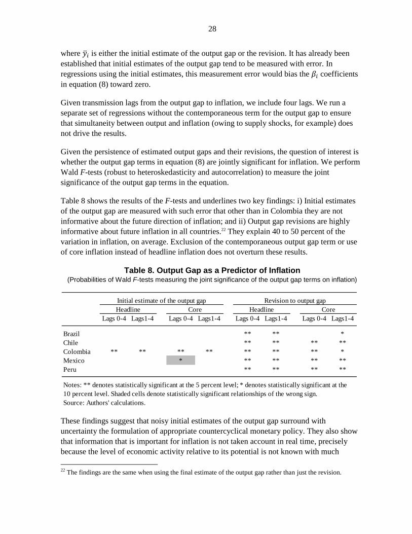
Table 8 shows the results of the F-tests and underlines two key findings: i) Initial estimates
of the output gap are measured with such error that other than in Colombia they are not
informative about the future direction of inflation; and ii) Output gap revisions are highly
informative about future inflation in all countries.22 They explain 40 to 50 percent of the
variation in inflation, on average. Exclusion of the contemporaneous output gap term or use
of core inflation instead of headline inflation does not overturn these results.
Table 8. Output Gap as a Predictor of Inflation (Probabilities of Wald F-tests measuring the joint significance of the output gap terms on inflation)
These findings suggest that noisy initial estimates of the output gap surround with
uncertainty the formulation of appropriate countercyclical monetary policy. They also show
that information that is important for inflation is not taken account in real time, precisely
because the level of economic activity relative to its potential is not known with much
22
The findings are the same when using the final estimate of the output gap rather than just the revision.
Lags 0-4 Lags1-4 Lags 0-4 Lags1-4 Lags 0-4 Lags1-4 Lags 0-4 Lags1-4
Brazil ** ** *
Chile ** ** ** **
Colombia ** ** ** ** ** ** ** *
Mexico * ** ** ** **
Peru ** ** ** **
Notes: ** denotes statistically significant at the 5 percent level; * denotes statistically significant at the
10 percent level. Shaded cells denote statistically significant relationships of the wrong sign.
Source: Authors' calculations.
Initial estimate of the output gap
Headline Core
Revision to output gap
Headline Core

29
certainty until long after policy decisions have been made. This underscores a key weakness
of monetary policy rules relying on real-time assessments of the cyclical position of the
economy.
V. SUMMARY AND CONCLUSIONS
This paper illustrates the wide range of uncertainty that is often associated with country
desks’ output gap assessments. We find that initial assessments of an economy’s cyclical
position overestimate the amount of slack in the economy, and that revisions are persistent,
especially during recessions. The paper also shows that only a small share of this uncertainty
can be explained by factors known to policymakers in real time, and that trying to explain
whether the initial estimate of the output gap will change sign is equally challenging. In
particular, we find that output gap revisions are positively associated with the absolute value
of the initial estimate of the output gap, and similarly, that real GDP growth surprises tend to
make subsequent output gap revisions larger. Evidence on the effects of macroeconomic
uncertainty on output gap revisions is mixed, while quality of data is a statistically significant
determinant of the revisions. In addition, countries with inflation targeting regimes have
lower output gap revisions.
Output gap data and revisions can be used to construct confidence intervals around any initial
or revised output gap estimate. The width of the confidence interval will vary by country, and
by the vintage of the revision, with a wider confidence interval for an initial estimate than for
a revised estimate. We find that, at the time of the initial estimate confidence intervals are
usually so large as to span positive and negative values for the output gap. In other words,
only in rare cases is there a high degree of certainty about whether policy should be
contractionary, neutral, or expansionary. These results underscore the challenges
policymakers face when using policy rules that depend on an assessment of the economy’s
cyclical position to set the value for a policy instrument.
The paper analyzes the implications of output gap uncertainty in the case of five Latin
American economies (Brazil, Chile, Colombia, Mexico and Peru) that adopted inflation
targeting as their monetary policy framework between 1999 and 2002. Assessing the
economy’s actual level of output relative to its potential is then a key policy input for these
countries, as the degree of spare capacity is typically an important predictor of future
inflation. We find that monetary policy reaction functions using revised (more accurate) real
GDP data result, in many cases, in values for the policy instrument that are significantly
different than those prescribed using initial estimates of the output gap. In addition, revised
estimates of the output gap are positively and significantly correlated with inflation,
suggesting that this information is not accounted for in real-time policy decisions.
These findings suggest that information that is important for inflation is not taken into
account by central banks in their policy decisions. This occurs, at least in part, because the
level of economic activity with respect to its potential is not known with much certainty until
30
long after policy decisions have been made. The difficulty in distinguishing between cyclical
fluctuations and shifts in the trend rate of growth underscores a key weakness of monetary
policy rules relying on real-time assessments of the cyclical position of the economy, even
when policymakers consult a large set of indicators.

31
Appendix I. Data
Table A1. Countries Included in the Analysis
Australia * + Denmark * + Greece * + Japan * + Norway * + Switzerland * +
Austria * + Finland * + Iceland * + Luxembourg * Portugal * + Turkey +
Belgium * + France * + Ireland * + Netherlands * + Spain * + United Kingdom * +
Canada * + Germany * + Italy * + New Zealand * + Sweden * + United States * +
Albania Cape Verde Gabon Latvia Papua New Guinea St. Vincent & Grens.
Algeria Chile Georgia Lebanon Paraguay Sudan
Angola China,P.R.: Mainland Ghana Lesotho Peru Suriname
Antigua and Barbuda China,P.R.:Hong Kong * Grenada Libya Philippines Swaziland
Argentina Colombia Guatemala Lithuania Poland + São Tomé & Príncipe
Armenia Congo, Republic of Guinea Macedonia, FYR Qatar Thailand
Azerbaijan, Rep. of Costa Rica Guyana Malaysia Romania Tonga
Bahamas, The Croatia Honduras Maldives Russian Federation Trinidad and Tobago
Bahrain, Kingdom of Cyprus * Hungary + Mauritania Samoa Tunisia
Barbados Czech Republic + India Mauritius Saudi Arabia Turkmenistan
Belarus Côte d'Ivoire Indonesia Mexico Senegal Ukraine
Belize Djibouti Iran, I.R. of Moldova Seychelles United Arab Emirates
Bhutan Dominica Israel * Mongolia Singapore * Uruguay
Bolivia Dominican Republic Jamaica Morocco Slovak Republic Uzbekistan
Bosnia & Herzegovina Ecuador Jordan Namibia Slovenia * Vanuatu
Botswana Egypt Kazakhstan Nicaragua Solomon Islands Venezuela, Rep. Bol.
Brazil El Salvador Kiribati Nigeria South Africa Vietnam
Brunei Darussalam Equatorial Guinea Korea, Republic of * Oman Sri Lanka Yemen, Republic of
Bulgaria Estonia Kuwait Pakistan St. Kitts and Nevis Zambia
Cameroon Fiji Lao People's Dem.Rep Panama St. Lucia
Bangladesh Central African Rep. Ethiopia Kyrgyz Republic Nepal Tanzania
Benin Chad Gambia, The Madagascar Niger Togo
Burkina Faso Comoros Guinea-Bissau Malawi Rwanda Uganda
Burundi Congo, Dem. Rep. of Haiti Mali Sierra Leone
Cambodia Eritrea Kenya Mozambique Tajikistan
Advanced economies
Emerging economies
Low income countries
Notes: Countries with an asterisk were included in WEO data regressions and those with a plus sign were included in OECD data regressions. Advanced
economies correspond to OECD member economies since 1990. Low income countries correspond to all countries with a GNI per capita of $1,045 or less in
2012. Emerging economies are all remaining economies in the sample.
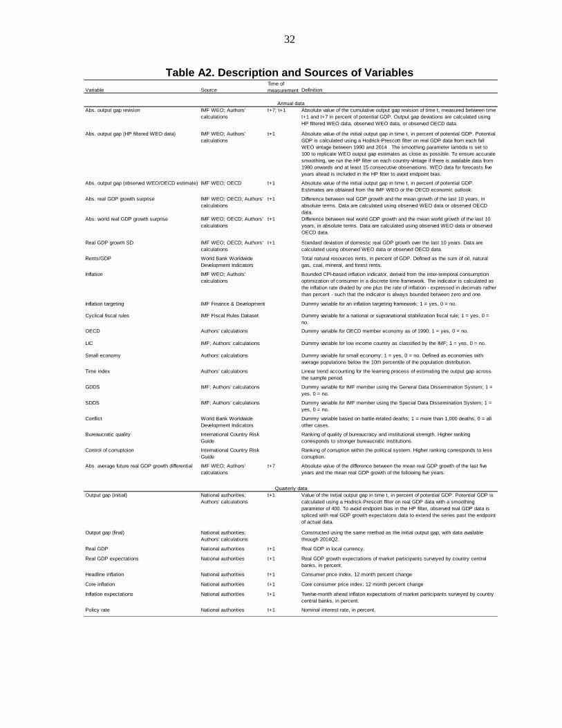
32
Table A2. Description and Sources of Variables
Variable Source
Time of
measurement Definition
Abs. output gap revision IMF WEO; Authors'
calculations
t+7; t+1 Absolute value of the cumulative output gap revision of time t, measured between time
t+1 and t+7 in percent of potential GDP. Output gap deviations are calculated using
HP filtered WEO data, observed WEO data, or observed OECD data.
Abs. output gap (HP filtered WEO data) IMF WEO; Authors'
calculations
t+1 Absolute value of the initial output gap in time t, in percent of potential GDP. Potential
GDP is calculated using a Hodrick-Prescott filter on real GDP data from each fall
WEO vintage between 1990 and 2014 . The smoothing parameter lambda is set to
100 to replicate WEO output gap estimates as close as possible. To ensure accurate
smoothing, we run the HP filter on each country-vintage if there is available data from
1980 onwards and at least 15 consecutive observations. WEO data for forecasts five
years ahead is included in the HP filter to avoid endpoint bias.
Abs. output gap (observed WEO/OECD estimate) IMF WEO; OECD t+1 Absolute value of the initial output gap in time t, in percent of potential GDP.
Estimates are obtained from the IMF WEO or the OECD economic outlook.
Abs. real GDP growth surprise IMF WEO; OECD; Authors'
calculations
t+1 Difference between real GDP growth and the mean growth of the last 10 years, in
absolute terms. Data are calculated using observed WEO data or observed OECD
data.
Abs. world real GDP growth surprise IMF WEO; OECD; Authors'
calculations
t+1 Difference between real world GDP growth and the mean world growth of the last 10
years, in absolute terms. Data are calculated using observed WEO data or observed
OECD data.
Real GDP growth SD IMF WEO; OECD; Authors'
calculations
t+1 Standard deviation of domestic real GDP growth over the last 10 years. Data are
calculated using observed WEO data or observed OECD data.
Rents/GDP World Bank Worldwide
Development Indicators
Total natural resources rents, in percent of GDP. Defined as the sum of oil, natural
gas, coal, mineral, and forest rents.
Inflation IMF WEO; Authors'
calculations
Bounded CPI-based inflation indicator, derived from the inter-temporal consumption
optimization of consumer in a discrete time framework. The indicator is calculated as
the inflation rate divided by one plus the rate of inflation - expressed in decimals rather
than percent - such that the indicator is always bounded between zero and one.
Inflation targeting IMF Finance & Development Dummy variable for an inflation targeting framework; 1 = yes, 0 = no.
Cyclical fiscal rules IMF Fiscal Rules Dataset Dummy variable for a national or supranational stabilization fiscal rule; 1 = yes, 0 =
no.
OECD Authors' calculations Dummy variable for OECD member economy as of 1990; 1 = yes, 0 = no.
LIC IMF; Authors' calculations Dummy variable for low income country as classified by the IMF; 1 = yes, 0 = no.
Small economy Authors' calculations Dummy variable for small economy; 1 = yes, 0 = no. Defined as economies with
average populations below the 10th percentile of the population distribution.
Time index Authors' calculations Linear trend accounting for the learning process of estimating the output gap across
the sample period.
GDDS IMF; Authors' calculations Dummy variable for IMF member using the General Data Dissemination System; 1 =
yes, 0 = no.
SDDS IMF; Authors' calculations Dummy variable for IMF member using the Special Data Dissemination System; 1 =
yes, 0 = no.
Conflict World Bank Worldwide
Development Indicators
Dummy variable based on battle-related deaths; 1 = more than 1,000 deaths, 0 = all
other cases.
Bureaucratic quality International Country Risk
Guide
Ranking of quality of bureaucracy and institutional strength. Higher ranking
corresponds to stronger bureaucratic institutions.
Control of corruptoion International Country Risk
Guide
Ranking of corruption within the political system. Higher ranking corresponds to less
corruption.
Abs. average future real GDP growth differential IMF WEO; Authors'
calculations
t+7 Absolute value of the difference between the mean real GDP growth of the last five
years and the mean real GDP growth of the following five years.
Output gap (initial) National authorities;
Authors' calculations
t+1 Value of the initial output gap in time t, in percent of potential GDP. Potential GDP is
calculated using a Hodrick-Prescott filter on real GDP data with a smoothing
parameter of 400. To avoid endpoint bias in the HP filter, observed real GDP data is
spliced with real GDP growth expectatons data to extend the series past the endpoint
of actual data.
Output gap (final) National authorities;
Authors' calculations
Constructed using the same method as the initial output gap, with data available
through 2014Q2.
Real GDP National authorities t+1 Real GDP in local currency.
Real GDP expectations National authorities t+1 Real GDP growth expectations of market participants surveyed by country central
banks, in percent.
Headline inflation National authorities t+1 Consumer price index, 12 month percent change
Core inflation National authorities t+1 Core consumer price index, 12 month percent change
Inflation expectations National authorities t+1 Twelve-month ahead inflaton expectations of market participants surveyed by country
central banks, in percent.
Policy rate National authorities t+1 Nominal interest rate, in percent.
Annual data
Quarterly data
33
References
Congressional Budget Office, 2001, CBO's Method for Estimating Potential Output: An
Update (Washington, D.C.).
Baxter, Marianne, and Robert G. King, 1999, “Measuring Business Cycles: Approximate
Band-Pass Filters for Economic Time Series,” The Review of Economics and
Statistics, Vol. 81(4), pp. 575-593.
Dreher, Axel, Silvia Marchesi, and James R. Vreeland, 2008, “The Politics of IMF
Forecasts,” Public Choice, Vol. 137, pp. 145-171.
Ho, Giang, and Paolo Mauro, 2014, “Growth: Now and Forever?” IMF Working Paper
14/117 (Washington: International Monetary Fund).
International Monetary Fund, 2010, “World Economic Outlook. Recovery, Risk and
Rebalancing,” October 2010, Washington, D.C.
Ley, Eduardo, and Florian Misch, 2013, “Real-Time Macro Monitoring and Fiscal Policy,”
Policy Research Working Paper 6303 (Washington: World Bank).
_______, 2014, “Output Data Revisions in Low-Income Countries,” paper presented at the
International Monetary Fund conference, “Macroeconomic Challenges Facing Low-
Income Countries: New Perspectives,” Washington, D.C., January.
Orphanides, Athanasios, 2001, “Monetary Policy Rules Based on Real-Time Data,” The
American Economic Review, Vol. 91, No. 4, pp. 964–985.
_______, and Simon van Norden, 2002, “The Unreliability of Output Gap Estimates in Real
Time,” The Review of Economics and Statistics, Vol. 84, pp. 569–583.
_______, and John C. Williams, 2007, “Robust Monetary Policy with Imperfect
Knowledge,” Journal of Monetary Economics, Vol. 54, pp. 1406–1435.
Ravn, Morten O., and Uhlig, Harald, 2002, “On Adjusting the Hodrick-Prescott Filter for the
Frequency of Observations,” The Review of Economics and Statistics, Vol. 82, No. 2,
pp. 371–375.
Roger, Scott, 2010, “Inflation Targeting Turns 20,” Finance & Development, Vol. 47
(March), pp. 46–49.
Timmermann, Allan, 2007, “An Evaluation of the World Economic Outlook Forecasts,” IMF
Staff Papers, Vol. 54, No. 1, pp. 1–33.
Woodford, Michael, 1999, “Optimal Monetary Policy Inertia,” The Manchester School
Supplement, pp. 1–35.
Related Documents