Project co-funded by the European Commission – DG Research 6 th Research Framework Programme TRIAS Sustainability Impact Assessment of Strategies Integrating Transport, Technology and Energy Scenarios Outlook for Global Transport and Energy Demand Deliverable 3 Version 1.1 September 2007 Co-ordinator: ISI Fraunhofer Institute Systems and Innovation Research, Karlsruhe, Germany Partners: IWW Institute for Economic Policy Research University of Karlsruhe, Germany TRT Trasporti e Territorio SRL Milan, Italy IPTS Institute for Prospective Technological Studies European Commission – DG-JRC, Seville, Spain

Welcome message from author
This document is posted to help you gain knowledge. Please leave a comment to let me know what you think about it! Share it to your friends and learn new things together.
Transcript

Project co-funded by the
European Commission – DG Research
6th Research Framework Programme
TRIAS Sustainability Impact Assessment of Strategies Integrating Transport, Technology and Energy Scenarios
Outlook for Global Transport and Energy Demand
Deliverable 3
Version 1.1
September 2007
Co-ordinator:
ISI Fraunhofer Institute Systems and Innovation Research, Karlsruhe, Germany
Partners:
IWW Institute for Economic Policy Research University of Karlsruhe, Germany
TRT Trasporti e Territorio SRL Milan, Italy
IPTS Institute for Prospective Technological Studies European Commission – DG-JRC, Seville, Spain

TRIAS
Sustainability Impact Assessment of Strategies Integrating Transport, Technology and Energy Scenarios
Deliverable information:
Deliverable no: 3
Workpackage no: 3/4
Title: Outlook for Global Transport and Energy Demand
Authors: Michael Krail, Wolfgang Schade, Davide Fiorello, Francesca Fermi, An-
gelo Martino, Panayotis Christidis, Burkhard Schade, Joko Purwanto,
Nicki Helfrich, Aaron Scholz, Markus Kraft
Version: 1.1
Date of publication: 26.09.2007
This document should be referenced as:
Krail M, Schade W, Fiorello D, Fermi F, Martino A, Christidis P, Schade B, Purwanto J, Helfrich
N, Scholz A, Kraft M (2007): Outlook for Global Transport and Energy Demand. Deliverable 3
of TRIAS (Sustainability Impact Assessment of Strategies Integrating Transport, Technology
and Energy Scenarios). Funded by European Commission 6th RTD Programme. Karlsruhe,
Germany.
Project information:
Project acronym: TRIAS
Project name: Sustainability Impact Assessment of Strategies Integrating Transport, Technology and Energy Scenarios.
Contract no: TST4-CT-2005-012534
Duration: 01.04.2005 – 30.06.2007
Commissioned by: European Commission – DG Research – 6th Research Framework Pro-gramme.
Lead partner: ISI - Fraunhofer Institute Systems and Innovation Research, Karlsruhe, Germany.
Partners: IWW - Institute for Economic Policy Research, University Karlsruhe, Germany.
TRT - Trasporti e Territorio SRL, Milan, Italy.
IPTS - Institute for Prospective Technological Studies, European Com-mission – DG-JRC, Seville, Spain.
Website: http://www.isi.fhg.de/trias/index.htm
Document control information:
Status: Accepted
Distribution: TRIAS partners, European Commission
Availability: Public
Filename: TRIAS_D3_Global_Outlook_TREN_Final.pdf
Quality assurance: reviewed Michael Krail
Coordinator`s review: reviewed Wolfgang Schade
Signature: Date: 25.09.2007
TRIAS D3 Outlook for Global Transport and Energy Demand - iii -
Table of contents:
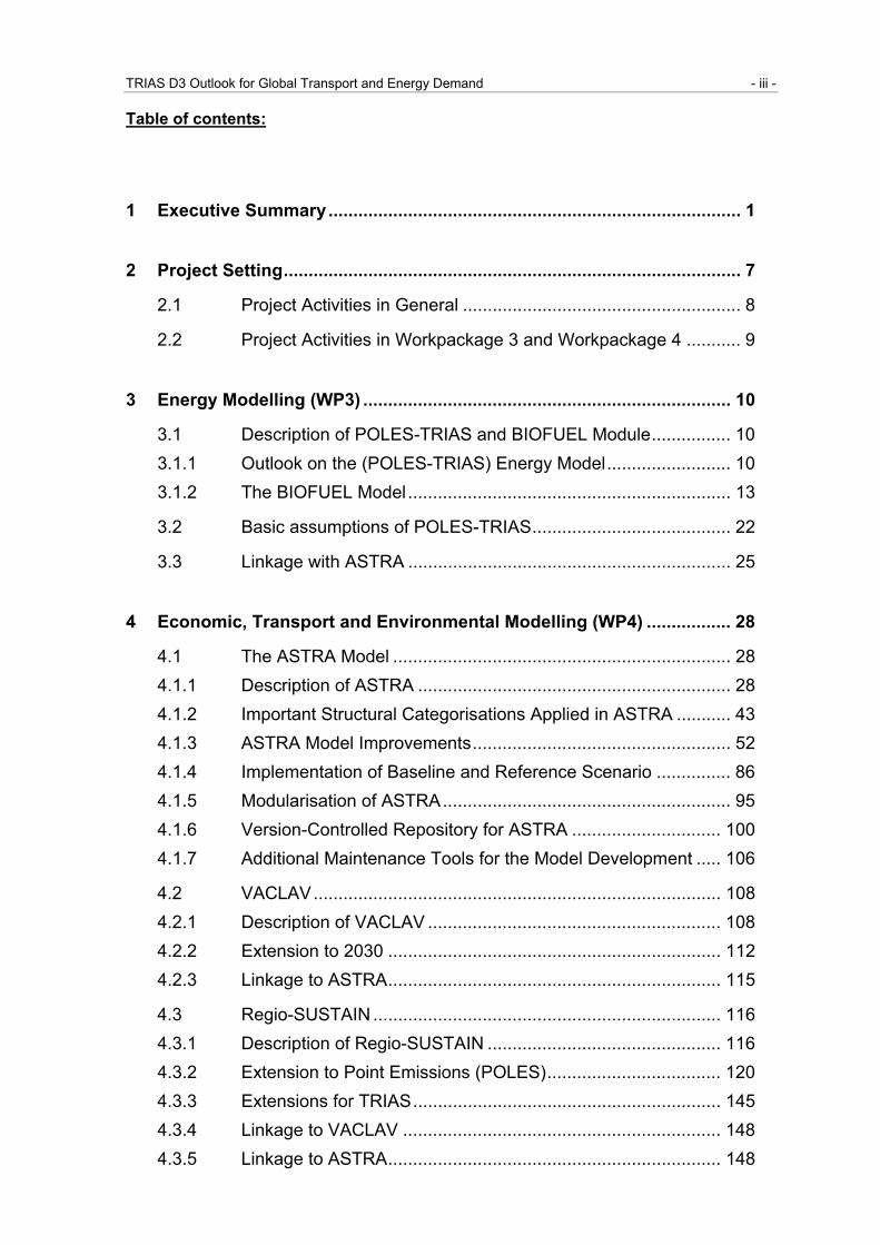
1 Executive Summary................................................................................... 1
2 Project Setting............................................................................................ 7
2.1 Project Activities in General ........................................................ 8
2.2 Project Activities in Workpackage 3 and Workpackage 4 ........... 9
3 Energy Modelling (WP3) .......................................................................... 10
3.1 Description of POLES-TRIAS and BIOFUEL Module................ 10 3.1.1 Outlook on the (POLES-TRIAS) Energy Model......................... 10 3.1.2 The BIOFUEL Model................................................................. 13
3.2 Basic assumptions of POLES-TRIAS........................................ 22
3.3 Linkage with ASTRA ................................................................. 25
4 Economic, Transport and Environmental Modelling (WP4) ................. 28
4.1 The ASTRA Model .................................................................... 28 4.1.1 Description of ASTRA ............................................................... 28 4.1.2 Important Structural Categorisations Applied in ASTRA ........... 43 4.1.3 ASTRA Model Improvements.................................................... 52 4.1.4 Implementation of Baseline and Reference Scenario ............... 86 4.1.5 Modularisation of ASTRA.......................................................... 95 4.1.6 Version-Controlled Repository for ASTRA .............................. 100 4.1.7 Additional Maintenance Tools for the Model Development ..... 106
4.2 VACLAV.................................................................................. 108 4.2.1 Description of VACLAV ........................................................... 108 4.2.2 Extension to 2030 ................................................................... 112 4.2.3 Linkage to ASTRA................................................................... 115
4.3 Regio-SUSTAIN ...................................................................... 116 4.3.1 Description of Regio-SUSTAIN ............................................... 116 4.3.2 Extension to Point Emissions (POLES)................................... 120 4.3.3 Extensions for TRIAS.............................................................. 145 4.3.4 Linkage to VACLAV ................................................................ 148 4.3.5 Linkage to ASTRA................................................................... 148

TRIAS D3 Outlook for Global Transport and Energy Demand - iv -
5 Baseline Scenario Results .................................................................... 149
5.1 Overview on major developments ........................................... 149
5.2 Demographic Development..................................................... 151
5.3 Economic Development .......................................................... 155
5.4 Transport System Trends........................................................ 163
5.5 Energy System Trends............................................................ 172
5.6 Environment ............................................................................ 179
6 Conclusions and Outlook...................................................................... 193
7 References.............................................................................................. 195

TRIAS D3 Outlook for Global Transport and Energy Demand - v -
List of tables
Table 1: POLES-TRIAS demand breakdown by main sectors ..................................... 13
Table 2: Country clusters and model assumptions....................................................... 21
Table 3: Summary of spatial categorisations used in different modules of ASTRA...... 44
Table 4: Summary of categorisation of NUTS II zones into functional zones in ASTRA for EU27+2 ............................................................................ 47
Table 5: Destinations reached by transport in each distance band .............................. 50
Table 6: 25 economic sectors used in ASTRA derived from the NACE-CLIO systematics ......................................................................................... 51
Table 7: Split of aggregate biofuel plant investments onto ASTRA sectors ................. 53
Table 8: Split of aggregate hydrogen plant investments onto ASTRA sectors ............. 54
Table 9: Conversion between SCENES flows and ASTRA purposes .......................... 57
Table 10: Conversion between SCENES modes and ASTRA modes.......................... 57
Table 11: Comparison between data stock and Eurostat total pkm per country in 1990 and 2000.................................................................................... 58
Table 12: Data found for car costs................................................................................ 60
Table 13: Equivalence table for private car costs ......................................................... 61
Table 14: Available data on bus costs. ......................................................................... 63
Table 15: Equivalence table for bus costs. ................................................................... 63
Table 16: Data estimated for long distance bus costs. ................................................. 64
Table 17: Data for Italian train costs derived from Cicini et al, (2005) .......................... 66
Table 18: Data for train costs, taken from UIC (1999) .................................................. 66
Table 19: Equivalence table for train costs................................................................... 67
Table 20: Original data on truck costs .......................................................................... 70
Table 21: Equivalence table for truck costs .................................................................. 70
Table 22: Conversion between ETIS commodity groups and ASTRA flows ................ 72
Table 23: Conversion between ETIS chain mode and ASTRA mode .......................... 73
Table 24: Comparison between data stock and Eurostat total tkm per country in 1990 and 2000.................................................................................... 74
Table 25: Diffusion of emission standards in ASTRA................................................... 85
Table 26: Applied deflators to harmonize data between models .................................. 86
Table 27: Trend of total transport cost by mode (passenger and freight)..................... 89
Table 28: Assumed car price development per technology.......................................... 91
TRIAS D3 Outlook for Global Transport and Energy Demand - vi -
Table 29: Assumed filling station infrastructure development for H2 and Bioethanol........................................................................................... 92
Table 30: Assumptions on emission reductions after Euro 7 for baseline scenario ..... 94
Table 31: List of modules and their associated models in ASTRA ............................... 96
Table 32: ASTRA merger files ...................................................................................... 99
Table 33: Multi-pollutant/multi-effect approach of the RAINS model .......................... 122
Table 34: POLES – RAINS-GAINS fuel type relationship .......................................... 129
Table 35: POLES – RAINS/GAINS sector type relationship for NOx stationary......... 130
Table 36: POLES – RAINS/GAINS sectors and fuel types relationship for PM10 stationary .......................................................................................... 132
Table 37: NACE Code included in EPER Database in Relation to Energy Sector in POLES Model ............................................................................... 135
Table 38: RAINS Sectors Related to Stationary Sources with Energy Combustion... 144
Table 39: Growth rates per year ................................................................................. 146
Table 40: Average yearly population growth rates ..................................................... 152
Table 41: Demographic changes per age class ......................................................... 155
Table 42: Change of car share(1) in the EU27 countries in the baseline..................... 166
Table 43: Biofuel production costs.............................................................................. 174
Table 44: NUTS III regions under consideration for the regional environmental assessment....................................................................................... 186

TRIAS D3 Outlook for Global Transport and Energy Demand - vii -
List of figures
Figure 1: Linkage and interaction of models in TRIAS. .................................................. 1
Figure 2: Major developments in the transport-energy-economic system of the EU27..................................................................................................... 3
Figure 3: Major developments in the transport and energy system of the EU27............ 4
Figure 4: Share of passenger car technology in EU27 ................................................... 5
Figure 5: NOx immissions in the Ruhr area (Baseline scenario for 2000)...................... 6
Figure 6: Linkage and interaction of models in TRIAS. .................................................. 8
Figure 7: POLES-TRIAS five modules and simulation process.................................... 11
Figure 8: POLES-TRIAS five vertical integration .......................................................... 12
Figure 9: Biofuel supply and demand shifts.................................................................. 14
Figure 10: Interaction of factors affecting supply and demand of biofuels (Wiesenthal forthcoming).................................................................... 16
Figure 11: Change of feedstock prices (Wiesenthal forthcoming) ................................ 17
Figure 12: Investment and total costs for different biofuels .......................................... 18
Figure 13: Member States interest to support biofuel consumption vs. interest to support feedstock production.............................................................. 20
Figure 14: Evolution of fuel price without VAT in EU-27............................................... 24
Figure 15: Population trend in ASTRA and POLES-TRIAS models ............................. 26
Figure 16: GDP trend in ASTRA and POLES-TRIAS model (ADAM trend) ................. 26
Figure 17: Data exchange between ASTRA, POLES-TRIAS and BIOFUEL models ................................................................................................ 27
Figure 18: Overview on the structure of the nine ASTRA modules .............................. 31
Figure 19: The consumption feedback loop in ASTRA and its impacts from transport.............................................................................................. 36
Figure 20: The investment feedback loop in ASTRA and its impacts from transport.............................................................................................. 37
Figure 21: The employment feedback loop in ASTRA and its impacts from transport.............................................................................................. 38
Figure 22: The government feedback loop in ASTRA and its impacts from transport.............................................................................................. 39
Figure 23: The export feedback loop in ASTRA and its impacts from transport........... 40
Figure 24: The freight transport feedback loops in ASTRA .......................................... 41
Figure 25: The passenger transport feedback loops in ASTRA ................................... 43

TRIAS D3 Outlook for Global Transport and Energy Demand - viii -
Figure 26: Overview on spatial differentiation in ASTRA.............................................. 48
Figure 27: Structure of the car-ownership effect on modal split ................................... 56
Figure 28: Car cost split................................................................................................ 59
Figure 29: Urban bus cost split ..................................................................................... 62
Figure 30: Non-local bus cost split................................................................................ 64
Figure 31: Train passenger cost split............................................................................ 65
Figure 32: Road freight cost split .................................................................................. 69
Figure 33: Train freight cost split .................................................................................. 71
Figure 34: New ASTRA passenger car categories ....................................................... 78
Figure 35: Drivers of Car Purchase Decision ............................................................... 79
Figure 36: Estimation of average distance to filling station........................................... 81
Figure 37: ASTRA car purchase model ........................................................................ 83
Figure 38: ASTRA car fleet model ................................................................................ 84
Figure 39: Example for car life cycle modelling in ASTRA VFT module....................... 85
Figure 40: Exogenous GDP growth trends of rest-of-the-world regions in ASTRA ...... 87
Figure 41: Baseline trend of total pkm.......................................................................... 90
Figure 42: Baseline trend of total tkm........................................................................... 90
Figure 43: A typical client/server system .................................................................... 101
Figure 44: The problem to avoid................................................................................. 102
Figure 45: The Lock, Modify, Unlock Solution ............................................................ 102
Figure 46: The Copy, Modify, Merge Solution ............................................................ 104
Figure 47: VACLAV rail network model ...................................................................... 111
Figure 48: VACLAV road network model.................................................................... 112
Figure 49: VACLAV rail network for 2030................................................................... 113
Figure 50: VACLAV road network for 2030 ................................................................ 114
Figure 51: Overview on the original structure of the Regio-SUSTAIN database. ....... 117
Figure 52: Example of land cover data ....................................................................... 119
Figure 53: Flow of information in the RAINS model.................................................... 123
Figure 54: EPER Data Structure................................................................................. 125
Figure 55: Overview on the structure of the enhanced Regio-SUSTAIN database for the TRIAS project ........................................................................ 147
Figure 56: Major developments in the transport-energy-economic system of the EU27................................................................................................. 150

TRIAS D3 Outlook for Global Transport and Energy Demand - ix -
Figure 57: Major developments in the transport and energy system of the EU27...... 151
Figure 58: Demographic development in EU27.......................................................... 153
Figure 59: Share of age classes on total population in EU27..................................... 153
Figure 60: Demographic changes in selected EU countries....................................... 154
Figure 61: Overview on major economic trajectories for EU27 .................................. 156
Figure 62: GDP trajectories for the individual EU15 countries ................................... 157
Figure 63: GDP trajectories for the individual EU12+2 countries ............................... 157
Figure 64: Change of exports of goods sectors for the EU27..................................... 159
Figure 65: Change of exports of service sectors for the EU27 ................................... 159
Figure 66: Change of production value of goods sectors in EU27 ............................. 160
Figure 67: Change of employment in goods sectors of EU27 .................................... 161
Figure 68: Change of employment in service sectors of EU27................................... 161
Figure 69: Trajectories of employment by sectors in EU27 ........................................ 162
Figure 70: Trajectories of different transport related investments in EU12 and EU15................................................................................................. 162
Figure 71: Baseline trend of total pkm........................................................................ 163
Figure 72: Baseline trend of total tkm......................................................................... 164
Figure 73: Baseline trend of Pass-km by mode of transport....................................... 165
Figure 74: Baseline trend of passenger mode split in the EU27 countries ................. 165
Figure 75: Baseline trend of Tonnes-km by mode of transport................................... 167
Figure 76: Baseline trend of freight mode split in the EU27 countries........................ 168
Figure 77: Overview on vehicle fleet trends in EU27.................................................. 170
Figure 78: Passenger car technology trends in EU27 ................................................ 171
Figure 79: Share of passenger car technology in EU27 ............................................. 172
Figure 80: EU27 total energy consumption (without electricity and transformation sector)............................................................................................... 173
Figure 81: Total world energy consumption by region (without electricity and transformation system) ..................................................................... 173
Figure 82: Biofuel production in the base scenario..................................................... 175
Figure 83: Share of biofuels to fuel demand............................................................... 176
Figure 84: EU27 fuel consumption per fuel type......................................................... 177
Figure 85: Consumption of bioethanol in EU15 countries .......................................... 178
Figure 86: Consumption of bioethanol in EU12+2 countries Figure ........................... 178

TRIAS D3 Outlook for Global Transport and Energy Demand - x -
Figure 87: EU27 air emission trends versus transport performance .......................... 180
Figure 88: EU27 CO2 emission trends per mode....................................................... 181
Figure 89: EU27 absolute CO2 emissions per mode ................................................. 182
Figure 90: EU27 NOx emission trends per mode ....................................................... 183
Figure 91: EU27 absolute NOx emissions per mode.................................................. 184
Figure 92: Share of CO2 emissions from electricity production in EU-27 countries .... 185
Figure 93: Ruhr area (Germany) as assessed in the TRIAS project (GoogleMaps, 2007)................................................................................................. 187
Figure 94: Andalusia (Spain) as assessed in the TRIAS project (GoogleMaps, 2007)................................................................................................. 187
Figure 95: NOx immissions in the Ruhr area (Baseline scenario for 2000)................ 190
Figure 96: PM immissions in the Ruhr area (Baseline scenario for 2000).................. 190
Figure 97: NOx immissions in Andalusia (Baseline scenario for 2000) ...................... 191
Figure 98: PM immissions in Andalusia (Baseline scenario for 2000)........................ 192

TRIAS D3 Outlook for Global Transport and Energy Demand - xi -
List of abbreviations
ASTRA Assessment of Transport Strategies AUT Austria BD Biodiesel BETOH Bioethanol BETOH Ligno Bioethanol from Lignocellulosic Biomass BIO Bioethanol driven cars (E85 including flexi-fuel cars) BLX Belgium and Luxemburg BLG Bulgaria BTL Biomass To Liquids CHE Switzerland CNG Compressed natural gas CO2 Carbon dioxide CYP Cyprus CZE Czech Republic DNK Denmark DPC1 Diesel cars with cubic capacity less than 2.0 litre DPC2 Diesel cars with cubic capacity more than 2.0 litre ELC Electric current driver cars EST Estonia ESP Spain EU European Union EU12 All new Member States acceded the EU in 2004 and 2007 EU12+2 All new Member States acceded the EU in 2004 and 2007 plus Norway and Swit-
zerland EU15 All members of the EU until 2003 EU25 All Member States of the EU despite Bulgaria and Romania acceded in 2007 EU27 All Member States of the EU in the year 2007 FIN Finland FC Fuel cell FRA France HUN Hungary G7 Group of Seven, meeting of finance ministers Gbl Giga barrel GBR Breat Britain/UK GDP Gross Domestic Product GER Germany GHG Greenhouse Gases GPC1 Gasoline cars with cubic capacity less than 1.4 litre GPC2 Gasoline cars with cubic capacity more than 1.4 and less than 2.0 litre GPC3 Gasoline cars with cubic capacity more than 2.0 litre GRC Greece GVA Gross value-added HYB Hybrid cars, gasoline/diesel and electric H2 Hydrogen IRL Ireland ITA Italy LAT Latvia LPG Liquefied petroleum gas LTU Lithuania

TRIAS D3 Outlook for Global Transport and Energy Demand - xii -
MLT Malta NACE General industrial classification of economic activities within the European com-
munities NGV Natural gas vehicle NLD The Netherlands NOR Norway NOx Nitrogen oxide NUTS Nomenclature of Territorial Units of Statistics OD Origin/Destination Pkm Passenger-kilometre PM Particulate matter POL Poland POP Population PRT Portugal ROM Romania RoW Rest-of-the-World countries SAM Social accounting matrice SEA Strategic environmental assessment SLO Slovenia SVK Slovakia SWE Sweden TFP Total factor productivity Tkm Ton-kilometre Vkm Vehicle-kilometre WP Work package VAT Value-added tax Yr Year
TRIAS D3 Outlook for Global Transport and Energy Demand - 1 -
1 Executive Summary
The main objective of the TRIAS project is to perform an integrated sustainability impact as-
sessment of transport, technology and energy scenarios. In order to fulfil the requirements of
an integrated sustainability impact assessment five models simulating economic, transport,
environment, energy and technology systems were linked in TRIAS. Finally, the linked models
are fed with technology scenarios as well as policies for transport and its energy supply. The
following five models were integrated and prepared for the implementation of scenarios:
• POLES and BIOFUEL covering the energy sector,
• ASTRA for modelling national economies, sectoral foreign trade and transport on an
aggregate level,
• VACLAV simulating detailed transport network impacts on NUTSIII level and
• Regio-SUSTAIN highlighting local environmental impacts for two selected European
regions.
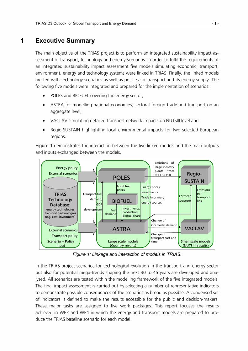
Figure 1 demonstrates the interaction between the five linked models and the main outputs
and inputs exchanged between the models.
POLES
ASTRA
Energy prices,
Investments
Trade in primary
energy sources
Large scale models (Country results)
Scenario + Policy Input
Energy policy
External scenarios
External scenarios
Transport policy
BIOFUEL
Fossil fuel prices
Investments, Production, Biofuel share
Fuel demand
VACLAV
Regio-
SUSTAIN
Emissions of large industry plants from POLES-EPER
Emissions per transport link
Change of transport cost and time
Change of
OD modal demand
Small scale models (NUTS III results)
Transport fuel
demand,
GDP
development
TRIAS Technology Database:
energy technologies transport technologies (e.g. cost, investment)
Car fleet
structure
Figure 1: Linkage and interaction of models in TRIAS.
In the TRIAS project scenarios for technological evolution in the transport and energy sector
but also for potential mega-trends shaping the next 30 to 45 years are developed and ana-
lysed. All scenarios are tested within the modelling framework of the five integrated models.
The final impact assessment is carried out by selecting a number of representative indicators
to demonstrate possible consequences of the scenarios as broad as possible. A condensed set
of indicators is defined to make the results accessible for the public and decision-makers.
These major tasks are assigned to five work packages. This report focuses the results
achieved in WP3 and WP4 in which the energy and transport models are prepared to pro-
duce the TRIAS baseline scenario for each model.

- 2 - Executive Summary
In the context of WP3 and WP4 several new features like the integration of alternative trans-
port technologies in the models, the update of data sources used for calibration and the ex-
tension of time horizon of model simulations until 2030 and 2050 were carried out. In addi-
tion to the development of interfaces linking the five models, significant effort has been in-
vested into two originally not foreseen tasks:
• A new BIOFUEL model was developed and linked with the POLES model. In order to
simulate biofuels scenarios this development was crucial for the TRIAS project.
• The ASTRA model was successfully split into modules in order to enable distributed
software development. For this purpose, a tool, the so-called ASTRA-Merger, was de-
veloped to link the separate modules of ASTRA into one integrated model again.
Major model improvements for TRIAS
The main improvements for the BIOFUEL and the POLES-TRIAS model consist in the develop-
ment of the BIOFUEL model itself and its linkages to the POLES-TRIAS model. With respect to
the relevant biofuel pathways, the BIOFUEL model performs the calculation of production
costs split by capital, operational and feedstock costs. In the next step, market prices of bio-
fuels and of fossil fuels calculated by POLES-TRIAS are linked together. This enables to derive
the level of production capacity and the production of biofuels, which are sold as blended
fuel or as pure biofuel. Besides costs, production and consumption of biofuels, the BIOFUEL
model derives also emissions in order to conduct a full assessment of policy instruments fos-
tering biofuels as transport fuels.
Several important improvements of the ASTRA model were realised in WP4 of the TRIAS pro-
ject. Regarding the simulation of technological scenarios the most important one was the
revision of the vehicle fleet model. Six new alternative car technologies - CNG, LPG, hybrid,
electric, bioethanol and hydrogen cars – were integrated in a new vehicle purchase model
driven by specific costs and filling station infrastructure. This task was completed in adding
the air emissions caused by alternative fuel cars with the help of specific emission factors in
the environmental module. Feedback loops were implemented simulating the technological
impacts in the macroeconomics and foreign trade model. Besides other significant innova-
tions motorisation levels were integrated as driver of passenger modal split and transport cost
calculations were disaggregated and revised.
The transport network model VACLAV has been extended to 2030 in regard of networks and
demand matrices. The latter has been achieved by adding a link to the ASTRA model and
using growth rate forecasts for passenger and freight demand. Furthermore detailed assign-
ment information is provided back to ASTRA for selected years.
Regio-SUSTAIN has been developed to assess the impacts of traffic-related emissions on a
regional scale. The model has been modified and applied to two case-study regions during
the TRIAS project, namely the Ruhr area (Germany) and Andalusia (Spain). Boundaries for the
two regions are based on the Nomenclature of Territorial Units of Statistics (NUTS). The out-
come of Regio-SUSTAIN is two-fold: On the one hand side local immissions and on the other
side the number of inhabitants affected by a special substance, such as NOx, PM or noise,
can be computed. For the TRIAS project Regio-SUSTAIN has been expanded to point emis-

TRIAS D3 Outlook for Global Transport and Energy Demand - 3 -
sions from stationary facilities. Furthermore, new components have been added to the model
for small-scale scenario analysis (e.g. demographic development, new vehicle emissions
classes, elevation model).
Major developments in TRIAS baseline scenario
The TRIAS baseline scenario provides trajectories for the analysed indicators until 2050. The
most suitable way to present a variety of indicators across different fields is to use indices,
which we calculate relative to the base year 2000. Figure 2 shows the major results of the
TRIAS baseline scenario that can be assigned to three different groups of indicators. The first
group includes indicators that remain stable or only show very moderate growth until 2050.
This includes population and employment, which both show a peak in the period 2025 to
2035 and then decline, but overall remain very close to the level of the year 2000. Transport
energy demand, transport CO2 emissions (life cycle perspective) and passenger performance,
which are the other three indicators of this group, increase by up to 50% until 2050. The
second group reveals a growth of about 200% until 2050. GDP and freight transport per-
formance belong to this group, which indicates that the models do not foresee a decoupling
between freight transport and GDP, but at least a relative decoupling between transport en-
ergy demand and GDP, which can be assigned to technological improvements including not
only improved energy efficiency of individual technologies but also switches between differ-
ent technologies. The last group in the figure represented by one indicator only reaches a
growth of more than 300%. This includes exports, which reveals that the models expect a
continuation of current globalisation trends leading to further specialisation of production in
different world regions and hence growing transport activity between different locations of
goods production.
Overview on major developments in the EU27
0
50
100
150
200
250
300
350
400
450
2000 2004 2008 2012 2016 2020 2024 2028 2032 2036 2040 2044 2048
Ind
ex [
year
200
0 =
100
]
Population
GDP
Exports
Employment
Freight performance
Passenger performance
Transport energy demand
Transport emiss ions CO2
Figure 2: Major developments in the transport-energy-economic system of the EU27

- 4 - Executive Summary
Taking a closer look at indicators of the transport and energy system in Figure 3 one can ob-
serve that for both freight and passenger transport the volumes grow slower than the per-
formance, which indicates that travel distances continue to grow, and in particular for pas-
senger transport this is the most relevant driver of continued growth. Despite stabilisation of
population the car fleet continues to grow significantly. One major reason is the catching-up
of the new EU member states joining the EU in the years 2004 and 2007 in terms of car-
ownership. Further in some countries income continues to grow strongly, which is one of the
strongest drivers of car purchase, and finally it seems that ASTRA generating this indicator is
more on the optimistic side of forecasts for this indicator.
Consumption and prices of the currently dominating fuels, gasoline and diesel, behave dif-
ferently. For gasoline, we observe a strongly rising fuel price as well as a sharp reduction of
demand reaching about -50% until 2030, which is due to both improved efficiency and fuel
switch of cars. For diesel the fuel price increase is much more moderate. Efficiency improve-
ments of trucks and buses, which consume a large share of diesel, remain lower then for cars
such that together with the strong growth of freight transport diesel fuel demand doubles
until 2050. In addition part of the fuel switch of cars is from gasoline cars to diesel cars,
which also drives the growth of diesel fuel demand.
Overview on major developments in the transport and energy system
0
50
100
150
200
250
300
350
2000 2004 2008 2012 2016 2020 2024 2028 2032 2036 2040 2044 2048
Inde
x (y
ear 2
000
= 10
0)
Freight volume
Freight performance
Passenger volumePassenger performance
Car fleet
Transport energy demandDiesel fuel price
Diesel fuel demand
Gasoline fuel priceGasoline fuel demand
Figure 3: Major developments in the transport and energy system of the EU27
Figure 4 presents the development of shares of each car technology on total EU27 car fleet
and clarifies the origin of increasing diesel fuel demand in EU27. The observed trend towards
diesel continues until 2030 account of gasoline technology. Especially the CNG technology,
which is promoted in several member states via initiatives, benefits from increasing diesel and
gasoline prices until 2024. In the following predicted natural gas price growth by POLES-
TRIAS leads to a strengthening of improved gasoline and alternative bioethanol technology.
According to cognitions made in other projects the TRIAS baseline scenario per definition
does not consider a successful diffusion of hydrogen cars into the EU27 markets until 2050.
Regarding the moderate growth of passenger transport performance (see Figure 3) and the

TRIAS D3 Outlook for Global Transport and Energy Demand - 5 -
technological improvements of alternative car technologies the reader might wonder about
the still increasing CO2 transport emissions of 50% until 2050. Finally this trend seems to be
realistic taking into account that freight transport performance is growing significantly until
2050 in EU27 and the fact that ASTRA does not consider alternative vehicle technologies to
be integrated in truck fleets. This leads to a movement of the main polluter of CO2 emissions
from passenger to freight transport.
EU27 development of car technologies
0%
5%
10%
15%
20%
25%
30%
35%
40%
45%
2000 2006 2012 2018 2024 2030 2036 2042 2048
Gasoline <1.4l
Gasoline >1.4l <2.0l
Gasoline >2.0l
Diesel <2.0l
Diesel >2.0l
CNG
LPG
Hybrid
Electric
Bioethanol
Hydrogen
Figure 4: Share of passenger car technology in EU27
Besides results on national level the TRIAS project intended to zoom into representative Euro-
pean case study regions to get an idea of the impacts on regional level. Figure 5 displays the
baseline results of the regional immission calculation with Regio-SUSTAIN for the transport
sector for nitrogen oxides. The major motorways with the highest transport loads in the Ruhr
area can be ascertained from the figures (the motorways A3 and A46). Both axis are mostly
used for long distance traffic, especially HGVs coming from the Dutch ports with destinations
in the South or East of Germany respectively Europe. The results are based on the assumption
of a constant average wind field of 225° (South-East direction) with an average speed of 2.5
m/s. Expert interviews have shown that the assumptions are acceptable.
The absolute values of this figure represent indicators for the situation in the region, as the
focus of TRIAS is on long-distance transport and energy pollutants only. Therefore, inner city
traffic and pollutants from households go behind the objectives of the project but should be
considered when analysing absolute values.
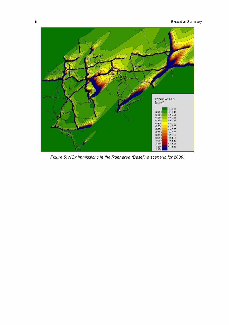
- 6 - Executive Summary
Figure 5: NOx immissions in the Ruhr area (Baseline scenario for 2000)

TRIAS D3 Outlook for Global Transport and Energy Demand - 7 -
2 Project Setting
The TRIAS project is performing a "Sustainability Impact Assessment of Strategies Integrating
Transport, Technology and Energy Scenarios". This means, the emerging fossil energy con-
straints, the potential technology lines for alternative fuels of transport and possible policies
to foster fuel switch of transport are combined for the TRIAS analyses and their potential
sustainability implications are assessed by the project team.
The project is co-funded by the European Commission DG Research and is undertaken by
four partners, with Fraunhofer Institute Systems and Innovation Research (ISI), Karlsruhe, tak-
ing the lead and collaborating with the Institute for Economic Policy Research (IWW) at the
University of Karlsruhe, TRT Trasporti e Territorio (TRT), Milan, and the Institute for Prospec-
tive Technological Studies (IPTS) of the European Commission DG JRC, Seville.
The strategic objectives of the TRIAS research project are
• Develop and test strategies to reduce greenhouse gas and noxious emissions from
transport, based on the trilogy (trias) of transport, technology and energy scenarios.
• Build the assessment on an integrated model-based approach, looking at environ-
mental, economic and social impacts (sustainability impact assessment).
• Consider the life-cycle implications of all strategies investigated.
The main scientific objective consists of the provision of a methodology for quantitative Sus-
tainability Impact Assessment (also known as Strategic Sustainability Analysis) considering
transport and energy sectors policies as well as scenario developments on the world scale,
like the development of oil prices, the global GDP growth rates or the potential of new tran-
sport technologies on world scale.
The project provides quantified scenarios of the potential of conventional and alternative
vehicle and fuel technologies until 2030 and - allowing for greater uncertainty - until 2050,
based on an integrated modelling approach that combines the techno-economic analysis of
transport technologies with the evaluation of environmental and socio-economic issues, as
well as issues related to the autonomy and security of energy supply.
TRIAS uses a set of established forecasting models and is applying them in an interlinked
manner to analyse the full picture of impacts induced by strategies including technology,
transport and energy scenarios. Investigated scenarios are developed in TRIAS both by build-
ing on external sources like national or international studies as well as other European pro-
jects and by using the inherent trends of the four TRIAS models. The four applied models act
at European scale (EU27) and include: POLES for energy modelling, ASTRA for transport and
economic modelling as well as integrated sustainability assessment, VACLAV for detailed
transport modelling and Regio-SUSTAIN for small scale analysis of environmental impacts,
which is limited to two selected European regions. As the energy supply system in particular
for fossil fuels is constituted as a world system the POLES model is also considering the global
energy system.
- 8 - Project Setting
2.1 Project Activities in General
The TRIAS project aspires to perform a Sustainability Impact Assessment of combined energy
and transport policies and scenarios. In order to provide reasonable advice for policy-making,
it is crucial to analyse the full picture of potential policies: in addition to the trajectory de-
scribing when a technology would first enter the market and how its market diffusion hap-
pens, an estimate of the required investments and the ways to finance these have to be part
of the analysis.
Giving an example: large scale changes of the energy supply system for transport might be
financed by charges collected from the transport users. Such charges would change the users
travel decisions altering the competitiveness of the different modes, which would have to be
reflected in a transport model to identify the full reactions to a policy. On the other hand,
investment and changes of transport prices affect the economic system, with different sec-
tors behaving in a different way. This requires using a sectoral economic model that is linked
with the transport system. Further, cost changes of long distance transport and lower de-
mand for fossil fuels would affect trade such that the applied model system should include a
trade model.
The research objective of TRIAS is then to provide such a combination of models that can be
fed with a broad range of technology scenarios as well as policies for transport and its energy
supply. To fulfil this research objective, three major tasks are designed:
1. Identification and development of scenarios for technological evolution in the transport
and energy sector but also for potential mega-trends shaping the next 30 to 45 years.
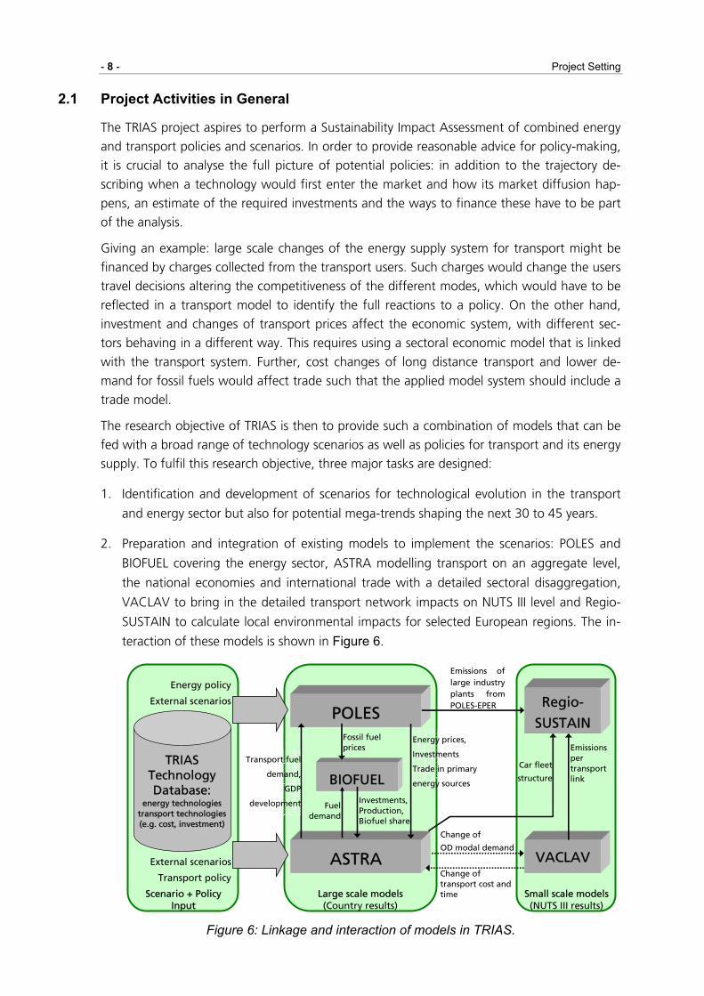
2. Preparation and integration of existing models to implement the scenarios: POLES and
BIOFUEL covering the energy sector, ASTRA modelling transport on an aggregate level,
the national economies and international trade with a detailed sectoral disaggregation,
VACLAV to bring in the detailed transport network impacts on NUTS III level and Regio-
SUSTAIN to calculate local environmental impacts for selected European regions. The in-
teraction of these models is shown in Figure 6.
POLES
ASTRA
Energy prices,
Investments
Trade in primary
energy sources
Large scale models (Country results)
Scenario + Policy Input
Energy policy
External scenarios
External scenarios
Transport policy
BIOFUEL
Fossil fuel prices
Investments, Production, Biofuel share
Fuel demand
VACLAV
Regio-
SUSTAIN
Emissions of large industry plants from POLES-EPER
Emissions per transport link
Change of transport cost and time
Change of
OD modal demand
Small scale models (NUTS III results)
Transport fuel
demand,
GDP
development
TRIAS Technology Database:
energy technologies transport technologies (e.g. cost, investment)
Car fleet
structure
Figure 6: Linkage and interaction of models in TRIAS.
TRIAS D3 Outlook for Global Transport and Energy Demand - 9 -
3. Sustainability Impact Assessment of the policies and scenarios. The scenarios are tested
with the interlinked five models and from each model a number of indicators is selected
to provide a picture of consequences of the scenarios as broad as possible. A condensed
set of indicators is defined to make the results accessible for the public and decision-
makers.
These three major tasks are organized in five technical work packages that are accompanied
by a number of workshops, in particular two open forums where results of TRIAS and similar
projects are discussed. The five work packages comprise:
• WP1 scenario screening of existing transport and energy scenarios;
• WP2 technology assessment and development of a technology, cost and investment
database for biofuel and hydrogen technologies;
• WP3 energy modelling preparing the POLES and BIOFUEL models for TRIAS;
• WP4 transport and economic modelling preparing the ASTRA, VACLAV and Regio-
SUSTAIN models for TRIAS;
• WP5 sustainability impact assessment analysing 10 different scenarios.
This deliverable presents the work undertaken and the results obtained in work packages
WP3 and WP4 of TRIAS.
2.2 Project Activities in Workpackage 3 and Workpackage 4
The major objective of WP3 and WP4 is to prepare the models for their application in TRIAS
and to produce the Baseline Scenario for each of the models. Preparing the models included
to add new features e.g. representing the alternative transport technologies in the models, to
update the data sources used for their calibration, to extend the time horizon of model simu-
lations until 2030 and 2050 and to establish the linkages between the models.
Significant effort has been invested into two originally not foreseen tasks: first, this is the
development of a new BIOFUEL model that is associated to the POLES model but could also
be integrated into the ASTRA model in the course of further development. Second, the
growth of the ASTRA model required to fully modularise it to enable distributed software
development and to make use of software tools and operational practices that support such
distributed software development. For this purpose, a complete software reengineering of
ASTRA was undertaken and a tool, the so-called ASTRA-Merger, was developed to link the
separate modules of ASTRA into one integrated model again.
Finally, a baseline scenario is developed using both external scenario assumptions and inter-
nal trends of the applied TRIAS models. Major external scenario assumptions come from the
ADAM project (Adaptation and Mitigation Strategies, EC 6FP), which provided GDP growth
trends until 2050 for the EU27 and the rest of the world. These trends were used as orienta-
tion for the GDP trends in ASTRA and POLES. Technology inputs were taken from the TRIAS
Technology Database developed in work package WP2 of TRIAS.

- 10 - Energy Modelling
3 Energy Modelling
3.1 Description of POLES-TRIAS and BIOFUEL Module
3.1.1 Outlook on the (POLES-TRIAS) Energy Model
The POLES model is a simulation model for the development of long-term (2050) energy
supply and demand scenarios for the different regions of the world. It has to be stated that in
the TRIAS project ASTRA and POLES are linked. Therefore, POLES runs with values that origi-
nate or are affected by other models. Hence, we name this model POLES-TRIAS. The devel-
opment of the model intends to fulfil five main objectives:
• to reduce the uncertainties in future developments of world energy consumption and
corresponding GHG emissions by the construction of baseline or reference scenarios;
• to provide elements for a global analysis of emission reduction strategies in an inter-
national perspective;
• to provide the key parameters of new energy technologies;
• to asses the marginal abatement costs for CO2 emissions and simulations of emission
trading system;
• to analyse the impacts of emission reduction strategies on the international energy
markets.
The model structure corresponds to a hierarchical system of interconnected modules and
articulates three level of analysis:
• international energy markets;
• regional energy balances;
• national energy demand, new technologies, electricity production, primary energy
production systems and CO2 sectoral emissions.
The main exogenous variables are the population and GDP, which was derived iteratively
with ASTRA, for each country / region, the price of energy being endogenised in the interna-
tional energy market modules. The dynamics of the model corresponds to a recursive simula-
tion process, common to most applied models of the international energy markets, in which
energy demand and supply in each national / regional module respond with different lag
structures to international prices variations in the preceding periods. In each module, behav-
ioural equations take into account the combination of price effects and of techno-economic
constraints, time lags or trends.
The development of such a disaggregate model of the world energy system has been made
possible by the availability of a complete International Energy Balance database (from 1971)
provided by ENERDATA and completed by techno-economic data gathered and organised at
IEPE. International economic databases for the key macro-economic variables used in the

TRIAS D3 Outlook for Global Transport and Energy Demand - 11 -
model have been provided by the CHELEM-CEPII database, in the framework of the LETS
network of the JOULE II program.
In POLES-TRIAS, the world is divided into fourteen main regions: North America, Central
America, South America, European Community (15 countries), Rest of Western Europe, For-
mer Soviet Union, Central Europe, North Africa, Middle-East, Africa South of Sahara, South
Asia, South East Asia, Continental Asia, Pacific OECD.
In most of these regions the larger countries are identified and treated, as concerns energy
demand, with a detailed model. In the current version these countries are the G7 countries
plus the countries of the rest of the European Union and five key developing countries: Mex-
ico, Brazil, India, South Korea and China. The countries forming the rest of the 14 above-
mentioned regions are dealt with more compact but homogeneous models.
Figure 7: POLES-TRIAS five modules and simulation process.
Vertical integration
For each region, the model articulates four main modules dealing with:
• Final Energy Demand by main sectors;
• New and Renewable Energy technologies;
• The Electricity and conventional energy and Transformation System;
• The Primary Energy Supply.

- 12 - Energy Modelling
As indicated in Figure 7, this structure allows for the simulation of a complete energy bal-
ance for each region.
FossilFuelSupply
Primary Energy
Fossil Fuels
ElectricityTransformationSystem
Primary Energy
NewRenewableEnergy
Net Final Energy
SectoralEnergyDemand
Final Energy
GDP POP
FossilFuelSupply
Primary Energy
Fossil Fuels
ElectricityTransformationSystem
Primary Energy
NewRenewableEnergy
Net Final Energy
SectoralEnergyDemand
Final Energy
GDP POP
Figure 8: POLES-TRIAS five vertical integration
Horizontal integration
While the simulation of the different energy balances allows for the calculation of import
demand / export capacities by region, the horizontal integration is ensured in the energy
markets module of which the main inputs are the import demands and export capacities of
the different regions. Only one world market is considered for the oil market (the "one great
pool" concept), while three regional markets (America, Europe, Asia) are distinguished for
coal and gas, in order to take into account for different cost, market and technical structures.
According to the principle of recursive simulation, the comparison of imports and exports
capacities for each market allows for the determination of the variation of the price for the
following period of the model. Combined with the different lag structure of demand and
supply in the regional modules, this feature of the model allows for the simulation of under-
or over-capacity situations, with the possibility of price shocks or counter-shocks similar to
those that occurred on the oil market in the seventies and eighties.
In the final energy demand module, the consumption of energy is divided into 11 different
sectors, which are homogenous from the point of view of prices, activity variables, consumer
behaviour and technological change. This is applied in each main country or region. The In-

TRIAS D3 Outlook for Global Transport and Energy Demand - 13 -
dustry, Transport and Residential-Tertiary-Agriculture blocks respectively incorporate 4, 4 and
3 such sectors:
Table 1: POLES-TRIAS demand breakdown by main sectors INDUSTRY Steel Industry
Chemical industry (+feedstock) Non metallic mineral industry Other industries (+non energy use)
STI CHI (CHF) NMM OIN (ONE)
TRANSPORT
Road transport Rail transport Air transport Other transports
ROT RAT ART OTT
RAS Residential sector Service sector Agriculture
RES SER AGR
In each sector, the energy consumption is calculated separately for substitutable techs and
for electricity, with a taking into account of specific energy consumption (electricity in electri-
cal processes and coke for the other processes in the steel-making, feedstock in the chemical
sector, electricity for heat and for specific uses in the Residential and Service sectors).
3.1.2 The BIOFUEL Model
The BIOFUEL model is based on a recursive year-by-year simulation of biofuel demand and
supply until 2050. For each set of exogenously given parameters an equilibrium point is cal-
culated at which the costs of biofuels equal those of the fossil alternative they substitute,
taking into account the feedback loops of the agricultural market and restrictions in the an-
nual growth rates of capacity. This equilibrium point is envisaged by market participants but
not necessarily reached in each year.
Increasing production of biofuels and a subsequent rise in feedstock demand has an impact
on the prices of biofuel feedstock, which in turn affects biofuel production through a feed-
back loop (Figure 9).

- 14 - Energy Modelling
S0
D0
D1
Q biofuel
P biofuel
subsidy Feedstock price change
S2
P1
P0
P2
Q2 Q1 Q0
Figure 9: Biofuel supply and demand shifts
First, the equilibrium point for the consumption of biofuels is identified. Keeping the other
factors constant, this would correspond to an equilibrium price for feedstock from each
pathway. At that level, a certain amount of feedstock would be produced as a result of the
agricultural market increasing or decreasing its supply compared to the reference case. The
change in the supply of biofuel feedstock will affect the area of cultivated land for these
feedstocks, the area for other products, as well as imports and exports of all related agricul-
tural products. As a result, prices will change and strongly influence the costs of biofuel pro-
duction as feedstock prices account for between around two thirds up to around 90% of
total production costs for conventional biofuels.
The reaction of the agricultural markets thus influences the production costs of biofuels and,
subsequently, the level of biofuel supply as shown schematically in Figure 9. This feedback is
modelled through a number of econometrically estimated equations, which are based on
information in the ESIM model simulation results and DG Agriculture. The assumed elastic-
ities for wheat, sugar beet, rapeseed, sunflower and lignocellulosic feedstock are 0.1, 0.1,
0.25, 0.2, 0.04, respectively.
It needs to be noted that the resource limits are exclusively taken into account through the
price effects, while upper physical limits for domestic biofuel feedstock supply were not con-
sidered. These necessitate a value judgement regarding e.g. the extent to which farmland
with a high nature value can be used for bioenergy cropping and whether food/fodder crop
cultivation shall be given higher priority than bioenergy production. The model delivers de-
tailed outcomes for the types of biofuels considered – biodiesel or ethanol, first or second
generation – with regard to production capacity and produced volumes, costs and well-to-
wheel emissions of greenhouse gases. Historical values for biofuel production, consumption
and production capacities are incorporated up to 2005.
The model focuses on the main production pathways of biofuels, namely biodiesel based on
rapeseed and sunflower and ethanol based on wheat and sugar beet, as well as advanced 2nd
generation pathways from lignocellulosic feedstock (i.e. ethanol and synthetic diesel BtL). For

TRIAS D3 Outlook for Global Transport and Energy Demand - 15 -
the 1st generation of biofuels the technical coefficients, costs and greenhouse gas emissions
are based on the deliverable D2 of the TRIAS project, with additional information from the
analysis carried out by the JEC study (JRC/EUCAR/CONCAWE 2006). Transportation costs in
TRIAS amount up to 20% of total costs while in the JEC study transportation cost are only in
the range of 5-6%. The lower transportation costs of the JEC study were taken into account.
For the 2nd generation the biofuel prices of TRIAS D2 were taken. Furthermore, technological
learning needs to be considered. However, this was only taken into account for 2nd genera-
tion biofuels as cost reductions in the production process of conventional biofuels are seen as
limited and lie within the range of uncertainties. Important cost reductions for 2nd generation
biofuels can be expected both in terms of the production process due to economies of scale
and more mature technologies and in terms of the feedstock, as current crops are not yet
optimised for their energy content. These effects can nevertheless be quantified only to a
very limited extent. For the purpose of the TRIAS scenarios, a cost reduction of about 20%
was assumed to occur until 2030 based on the TRIAS D2 values for 2010. As the cost reduc-
tion is dependent on the produced amount of biofuel the cost reduction varies between sce-
narios.
Figure 10 summarises the way the different factors interact. Impacts are traced in the various
sectors. The chart is restricted to the EU domestic biofuel market. Regarding imports, biofuel
prices are given as exogenous variables as well as their maximum penetration levels. Other
main exogenous parameters include
• Selection of biofuel production pathways;
• Production costs and maturity factors (learning of new production technologies);
• Well-to-wheel emissions of greenhouse gases;
• Development of oil prices and subsequently the fossil fuel prices;
• Elasticities of the raw material prices;
• Transport fuel demand.
Demand
Fossil fuel prices
Fuel demandTransport demandEnergy markets
(e.g. oil prices)
Biofuel prices
Convfuel price
Feedstock demand
Feedstock prices
Suitability (high/low blends)
Agricultural production
Production
Productioncapacity
Productioncosts
Emissions of greenhouse gases
Biofuels Module
Demand
Fossil fuel prices
Fuel demandTransport demandEnergy markets
(e.g. oil prices)
Biofuel prices
Convfuel price
Feedstock demand
Feedstock prices
Suitability (high/low blends)
Agricultural production
Production
Productioncapacity
Productioncosts
Emissions of greenhouse gases
Biofuels Module

- 16 - Energy Modelling
Figure 10: Interaction of factors affecting supply and demand of biofuels (Wiesenthal forth-
coming)
The model determines the penetration of biofuels as a function of final price of biofuels rela-
tive to the pump price of fossil fuels. These are affected by the prices of oil and raw materials
as well as the production costs that each alternative pathway entails (depending on capital
costs, feedstock prices, load factors etc.)
The relation of biofuel production costs to fossil prices excluding taxes is considered as an
incentive for investors to install additional production capacities, which in return leads to an
increased amount of biofuels produced. The additional installed capacity per year depends on
the distance to the equilibrium point (and thus the profit margin) and starts from historical
values: the average annual growth rate of biodiesel and bioethanol capacity was about 44%
and 69% over the period 2002 to 2006, respectively, and prospects for currently planned
projects indicate that similar rates are likely to continue also for the coming two years.
The main factors that determine the equilibrium point via influencing the cost ratio of biofu-
els and fossil fuels are oil prices, distribution costs and feedstock prices:
Oil prices influence the level of biofuel deployment as they are directly linked to fossil fuel
prices. On the other hand, they influence biofuel production costs for which energy costs
account for up to 15%. Besides, there is a limited, yet not negligible impact of oil prices on
the feedstock costs, which is taken from the JEC study (JRC/EUCAR/CONCAWE 2006).
Once the biofuel penetration exceeds a certain share and passes from low blends to higher
blends or pure biofuels, additional costs occur due to distribution and blending and poten-
tially adaptation of car engines.
Increasing production of biofuels and a subsequent rise in feedstock demand has an impact
on the prices of biofuel feedstock, which in turn affects biofuel production through a feed-
back loop. First, the equilibrium point for the consumption of biofuels is identified. Keeping
the other factors constant, this would correspond to an equilibrium price for feedstocks from
each pathway. At that level, a certain amount of feedstock would be produced as a result of
the agricultural market increasing or decreasing its supply compared to the reference case.
The change in the supply of biofuel feedstock will affect the area of cultivated land for these
feedstocks, the area for other products, as well as imports and exports of all related agricul-
tural products. As a result, prices will change and strongly influence the costs of biofuel pro-
duction as feedstock prices account for between around two thirds up to around 90% of
total production costs for conventional biofuels. The reaction of the agricultural markets con-
sequently influences the production costs of biofuels and, subsequently, the level of biofuel
supply and demand. This feedback is modelled through a number of econometrically esti-
mated equations, which are based on information in the ESIM model simulation results for
the agricultural sector and DG Agriculture. It needs to be noted that the resource limits are
exclusively taken into account through the price effects, while upper physical limits were not
considered.

TRIAS D3 Outlook for Global Transport and Energy Demand - 17 -
The following figure illustrates this effect: changes in feedstock prices are shown for a sce-
nario that assumes a biofuel quota of 10% to be reached by 2020, relative to a scenario that
assumes no further increase as of today.
0% 5% 10% 15% 20% 25% 30% 35%
Wheat
Rapeseed
Sunflower
Feedstock price increase between 10% obligation and baseline
2020
2010
Figure 11: Change of feedstock prices (Wiesenthal forthcoming)
The simulation results demonstrate the high interdependence of biodiesel feedstock prices on
biodiesel consumption. The feedback on ethanol feedstock prices remains limited, at least for
2010. Beyond 2010, the price increase for wheat can be explained by the much faster uptake
of ethanol compared to biodiesel. The main reason behind the different reaction of the etha-
nol and biodiesel markets is the fact that the supply curves of the two markets differ consid-
erably. There are large differences between biodiesel and bioethanol production in terms of
the share of the consumption of agricultural commodities for biofuel production compared
to the consumption of the same commodities for other uses, and the presence of global
markets.
In the case of rapeseed, 58% of the total harvested volume was used for biodiesel produc-
tion in 2006 (EC 2006). Total rapeseed consumption in the EU corresponds to one third of
the world production and is three times the size of the net international trade. Rapeseed and
rapeseed oil are therefore very responsive to changes in demand and an increase in biodiesel
production leads to a steep increase in their prices. The use of sunflower for biofuels repre-
sents a quarter of the total EU market for sunflower, a smaller but still significant share. The
repercussions of rapeseed and sunflower use for biofuels reach the food and animal feed
industry that also use their oils and meals as input. The recent rise in demand because of bio-
fuels has already now led to significant fluctuations in consumption, imports and prices of
inputs and final products for the related sectors. Alternatives do exist, mainly soybean and
soybean oil, coconut oil and palm oil, soybean meal and tapioca, but restrictions in interna-
tional trade and biofuel quality requirements limit the options considerably.
On the contrary, only about 1.5 percent of the total EU-25 cereals production and some 5%
of sugar beet production were used as feedstock for bioethanol in 2006. The impact of the
increased demand for bioethanol on the prices of cereals and sugar will be more limited than
for biodiesel. In addition, the reform of the Common Agricultural Policy (CAP) is expected to
create negative pressure on sugarbeet prices and/or free additional agricultural land for pro-
duction of cereals. Finally, it needs to be noted that unlike for biodiesel, there is already a
global market with the EU consumption and trade representing only a small share of world
production and international trade.

- 18 - Energy Modelling
So far, capital grants to support investment in biofuel production plant facilities played only a
limited role in promoting biofuels. This is mainly due to the relatively low investment costs
compared to the operation and maintenance costs of first generation biofuels (see Figure 12).
If, for example, a typical large biodiesel plant with investment costs of 15-20 Mio Euros was
supported with 10 Mio Euros, this would affect the biodiesel production costs by mere 0.01
€ per litre.
0
200
400
600
800
1000
1200
biodiesel fromrape
ethanol fromwheat
ethanol fromsugar beet
BTL ligno-cellulosicethanol
EUR/
toe
capital costs total costs
Figure 12: Investment and total costs for different biofuels
This may change drastically with advanced biofuels as the investment of the processing facili-
ties make a higher share of the total production costs of biofuels. Here, the investment sup-
port can be used to steer the type of biofuels produced in order to e.g. accelerate the market
introduction of advanced biofuels.
With this model structure, the development of biofuels deployment up to the equilibrium
point can be calculated for various sets of exogenous assumptions. In particular, the impacts
of different policy instruments on the deployment and mix of different biofuels and the
economy can be simulated, which is the main focus of the TRIAS analysis. The main imple-
mentation measures examined in the TRIAS scenarios include the following:
• A carbon permit price or carbon tax increasing from 0 (2010) to 30 €/t CO2 in 2030
and remains of this value till 2050. The value of 30 €/t CO2 is derived from a climate
change scenario that assumes a 21% domestic reduction of GHG emissions in the EU
by 2020 (EC 2007).
• Subsidies for investments in new capacity. This is analysed as a possible measure in
order to accelerate the deployment of advanced biofuel production technologies,
which may be desired due to their larger GHG emission benefits or potential.
• Quotas (obligation) differentiated according Member States for fuel suppliers to sell a
certain share of total sales as biofuels.
To determine the levels of the quota of the biofuel shares a clustering of Member States was
conducted (Figure 13). The TRIAS biofuel scenarios were also looked at on a Member State
base, which will be described in the following. For that purpose, Member States were

TRIAS D3 Outlook for Global Transport and Energy Demand - 19 -
grouped into clusters according to their potential in producing biofuel feedstock and their
interest in increasing biofuel consumption (Bekiaris 2007, Wiesenthal forthcoming).
So far, the European biofuel market is carried by a limited number of Member States. In
2005, only 4 (Spain, Sweden, Germany, France) and 3 Member States (Germany, France,
Italy) produced 80 % of the total EU ethanol and biodiesel production, respectively. In terms
of biofuel consumption, only Germany and Sweden achieved a market share of 2% or above
of total transport fuels by 2005. A number of other Member States are only recently imple-
menting national biofuel policies that will allow them achieving their national biofuel targets.
Despite the converging markets, it is likely to assume that the speed of the market deploy-
ment of biofuel and the eventual levels reached will continue to differ among Member
States. This will certainly depend on a Member States interest in either producing the biofuel
feedstock and/or the consumption of biofuels, depending on a number of country-specific
factors.
Having in mind the main drivers for setting up a biofuels policy, the overall economic
strength of a country combined with energy demand in transport and the importance of the
agricultural sector were seen as the most relevant characteristics of a country with regard to
biofuels. Even though all of these factors influence a country's interest in promoting biofuels
together with additional factors such as collaboration of the domestic car manufacturers or a
country's interest in pushing innovative biofuel technologies, a rough distinction can be made
between the interest in increasing cultivation of biofuel feedstock and consumption of biofu-
els.
Biofuel Consumption can be translated as the potential interest of a country to support the
use of biofuels domestically in order to reduce its oil dependency or for environmental rea-
sons (such as the reduction of greenhouse gases). There are examples of countries that can-
not produce excessive feedstock for biofuels production, but their energy demand and de-
pendency on energy – and specifically oil - imports is such that it is advisable to support con-
sumption of biofuels. Typical example of such a country is Germany, which, in spite of the
fact that it cannot cover all its needs in biodiesel, also needs to import from other countries
to satisfy the domestic demand.
Feedstock Production on the other hand is the potential interest of a country to support
feedstock production for biofuels. Again there are cases of countries that have great poten-
tial for cultivation of feedstock and an important agricultural sector although their potential
interest in biofuel consumption may not be that advanced. Typical examples of such coun-
tries are the Eastern European block members.
The indicator-based exercise results in the clustering of Member States as shown in Figure 13.
From the perspective of feedstock production, particularly Lithuania, Denmark, Poland, Hun-
gary and France can be classified as countries with an elevated interest in agricultural produc-
tion. As such, they are candidates for being interested in increasing domestic production of
biofuels. Nevertheless, this also depends on the competitiveness of conventional agricultural
products, which determines whether there is a need for the agricultural sector to switch to
alternative products. On the other hand, Member States that combine the economic capabil-
ity (high GDP) with high transport energy demand and related oil import dependency as well
as elevated CO2 emissions are likely to have a greater interest in increasing biofuels con-

- 20 - Energy Modelling
sumption. According to this indicator, most of the pre-2004 EU-15 Member States could
have an elevated interest in increasing the consumption of biofuels, led by Luxembourg and
followed by Germany, Ireland and France.
2
3
3
4
4
1 2 3 4
Possible interest in feedstock production
Poss
ible
inte
rest
in b
iofu
el c
onsu
mpt
ion
MT
IE
LU
BE
CZ
DK
DE
EE
GR
ES
FR
ITCY
LVLT
HU
NL
PL
PTSL
SV
FI
SE
UKAT
1 2
34
Figure 13: Member States interest to support biofuel consumption vs. interest to support
feedstock production
Not surprisingly most of the new Member States show a large potential of biofuel produc-
tion, particularly in relation to their transport fuel demand (Figure 13). They would not only
be self-sufficient so as to meet the 2010 biofuel target without any imports, but have a con-
siderable export potential. The export potential is further stressed by the fact that they may
lack the finance to support the creation of large domestic biofuel consumption. Some coun-
tries have started to create a biofuel policy (e.g. Czech Republic, Poland and Slovakia). How-
ever, biofuels are often rather exported than used domestically.
Luxembourg, Germany, Belgium, the Netherlands, Italy, Austria and United Kingdom are
countries with a relatively high economic strength but with a limited potential in arable land.
These countries have limited means to produce domestic feedstock, but may be interested to
import feedstock. The option of importing biofuels is supported by the factor that these
Member States (except for Luxembourg) host important harbours.
There are only few Member States that combine a high production potential with an elevated
interest in the consumption of biofuels. These comprise mainly France, Ireland and Finland,
and to a lesser extent Spain, Sweden and Cyprus.
Most of these Member States have implemented an ambitious biofuel policy, with the excep-
tion of Finland, Ireland and Denmark that considers the use of biomass for heat and power
production a favourable option compared with biofuels. France has been the leading player
on biofuels in Europe in the 1990s, driven by the strong agricultural and industrial sectors.
From 2000 biofuel share on the market was controlled by an accreditation (quota) system,
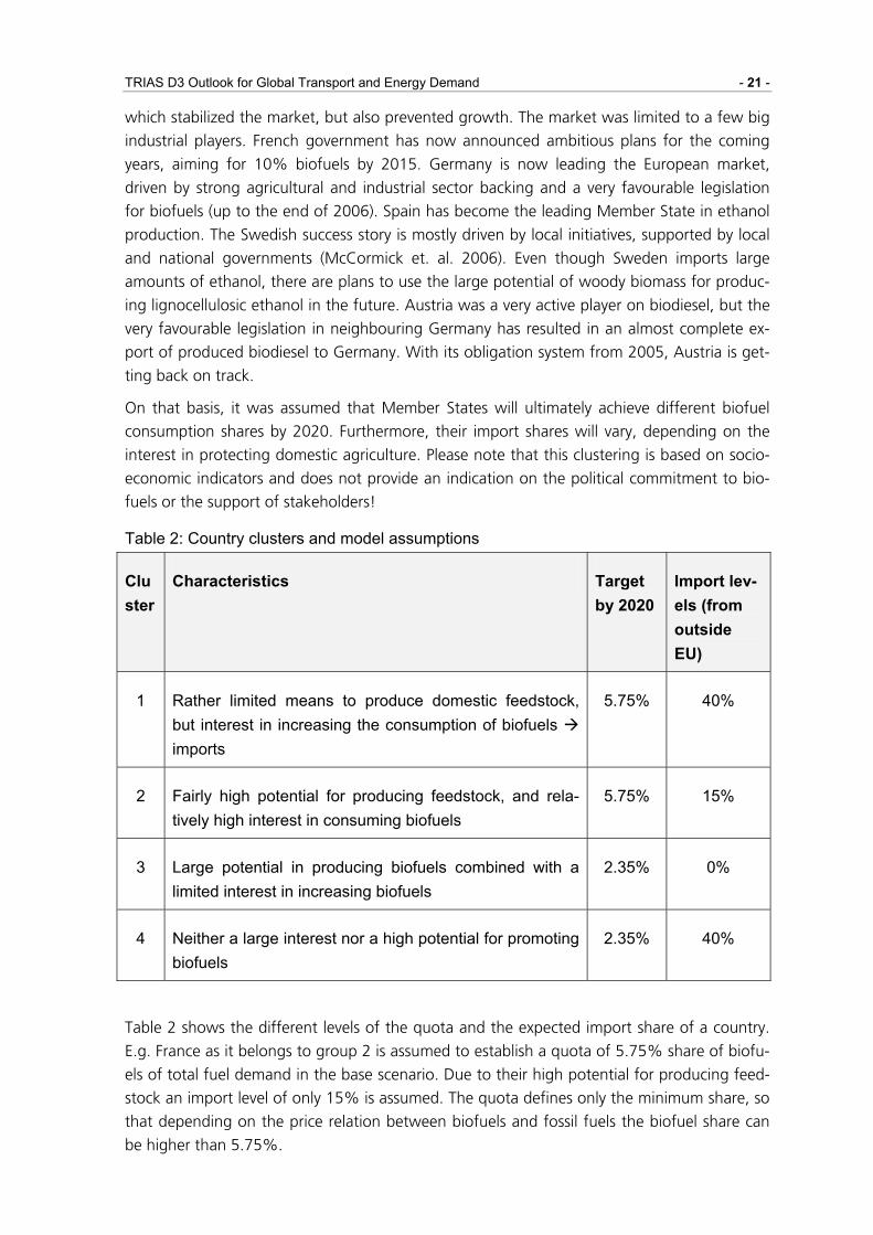
TRIAS D3 Outlook for Global Transport and Energy Demand - 21 -
which stabilized the market, but also prevented growth. The market was limited to a few big
industrial players. French government has now announced ambitious plans for the coming
years, aiming for 10% biofuels by 2015. Germany is now leading the European market,
driven by strong agricultural and industrial sector backing and a very favourable legislation
for biofuels (up to the end of 2006). Spain has become the leading Member State in ethanol
production. The Swedish success story is mostly driven by local initiatives, supported by local
and national governments (McCormick et. al. 2006). Even though Sweden imports large
amounts of ethanol, there are plans to use the large potential of woody biomass for produc-
ing lignocellulosic ethanol in the future. Austria was a very active player on biodiesel, but the
very favourable legislation in neighbouring Germany has resulted in an almost complete ex-
port of produced biodiesel to Germany. With its obligation system from 2005, Austria is get-
ting back on track.
On that basis, it was assumed that Member States will ultimately achieve different biofuel
consumption shares by 2020. Furthermore, their import shares will vary, depending on the
interest in protecting domestic agriculture. Please note that this clustering is based on socio-
economic indicators and does not provide an indication on the political commitment to bio-
fuels or the support of stakeholders!
Table 2: Country clusters and model assumptions
Cluster
Characteristics Target by 2020
Import lev-els (from outside EU)
1 Rather limited means to produce domestic feedstock, but interest in increasing the consumption of biofuels imports
5.75% 40%
2 Fairly high potential for producing feedstock, and rela-tively high interest in consuming biofuels
5.75% 15%
3 Large potential in producing biofuels combined with a limited interest in increasing biofuels
2.35% 0%
4 Neither a large interest nor a high potential for promoting biofuels
2.35% 40%
Table 2 shows the different levels of the quota and the expected import share of a country.
E.g. France as it belongs to group 2 is assumed to establish a quota of 5.75% share of biofu-
els of total fuel demand in the base scenario. Due to their high potential for producing feed-
stock an import level of only 15% is assumed. The quota defines only the minimum share, so
that depending on the price relation between biofuels and fossil fuels the biofuel share can
be higher than 5.75%.
- 22 - Energy Modelling
3.2 Basic assumptions of POLES-TRIAS
POLES-TRIAS provides an image of the energy scene to 2050 as resulting from the continua-
tion of on-going trends and structural changes in the world economy. This projection has
been developed with the POLES-TRIAS model. The Base scenario of POLES-TRIAS is quite simi-
lar to the Reference scenario being developed in the World Energy Technology Outlook–2050
or WETO-H2 study1. Main differences occur due to changes in GDP (which is calculated itera-
tively in combination with ASTRA) and due to a lower supply and demand for hydrogen in
the Base scenario of POLES-TRIAS. From the identification of the drivers and constraints in the
energy system, the model allows to describe the pathways for energy development, fuel sup-
ply, greenhouse gas emissions, international and end-user prices, from today to 2050.
The approach combines a high degree of detail in the key components of the energy systems
and a strong economic consistency, as all changes in these key components are largely de-
termined by relative price changes at sectoral level. As explained in the previous section, the
model identifies 46 regions of the world, with 22 energy demand sectors and about 40 en-
ergy technologies – now including generic “very low energy” end-use technologies, such as:
• Carbon capture and storage options as add-ons to plants burning fossil fuel to make
electricity or hydrogen
• Distributed electricity production, with or without cogeneration, from fossil fuel, re-
newable energy or hydrogen
• Low and very low energy buildings with significantly improved thermal performances
(meaning a reduction by a factor of 2 to 4 from the consumption of present buildings
in each region); these can even be “positive energy buildings” when photovoltaic sys-
tems are integrated into the design
The main exogenous inputs to the Baseline projection relate to: world population and eco-
nomic growth as the main drivers of energy demand; oil and gas resources as critical con-
straints on supply and the future costs and performances of energy technology that define
the feasible solutions. In all cases, the projected trends extrapolate existing structural
changes; this in no way implies, as is illustrated below, a uniform development of the world
economic and energy system.
An important aspect of the projections performed with the POLES-TRIAS model is that they
rely on a framework of permanent competition between technologies with dynamically
changing attributes. The expected cost and performance data for each critical technology are
gathered and examined in a customised database that organises and standardises the infor-
mation in a manner appropriate to the task.
1 http://ec.europa.eu/research/energy/pdf/weto-h2_en.pdf

TRIAS D3 Outlook for Global Transport and Energy Demand - 23 -
Critical Assumptions
Population
World population is expected to grow at a decreasing rate to 8.9 billions in 2050. After
2030, the population in several regions of the world decreases – including Europe and China.
Economic growth
The rate of economic growth in industrialised regions converges to 2.3%/yr in the very long
run. Growth in Asian emerging economies falls significantly after 2010, while conversely it
accelerates in Africa and the Middle East. As a result, global economic growth is expected
progressively to slow from 4.0%/yr in the 2001-2010 period to 2.8%/yr between 2010 and
2030 and then 2.5%/yr until 2050. Total world GDP in 2050 is more than three times the
present GDP.
World fossil fuel resources
Nowadays, the availability of oil and gas resources in the next decades is increasingly ques-
tioned. The accumulated production of oil to date is 900 Gbl. The assumption in this study is
that there remain almost 1 100 Gbl of identified reserves and slightly more than 600 Gbl of
resources that have not yet been identified. Higher recovery rates through technological pro-
gress are expected to extend the Ultimate Recoverable Resource base from 2700 Gbl today
to 3500 Gbl in 2050.
Energy Supply and Prices
The world oil production increases from around 30 Giga barrel in 2006 to around 44 Giga
barrels in 2034 before remains at that level until the end of the period (2050). About similar
trend can be expected to occur in the world natural gas supply, which will increase from
around 2.8 Gtoe in 2006 to reach around 4 Gtoe in the early 2030 and stays on that level
until 2050. As consequences, the average natural gas and gasoline prices (without VAT) in
EU-27 are expected to increase by around 40% between 2006 and 2050. Diesel price will
also increase but in a much slower rate.
The electricity production in EU-27 is expected to increase steadily by about 3.3% per year
from 2006 to 2050. In 45 year-period the average electricity price in EU-27 is expected to
increase by mere 4%.

- 24 - Energy Modelling
80
90
100
110
120
130
140
150
2000 2005 2010 2015 2020 2025 2030 2035 2040 2045 2050 2055
Inde
x
CNGDieselGasolineElectricity
Figure 14: Evolution of fuel price without VAT in EU-27
Energy technologies
Technology development will be critical in the shaping the future energy system. A thorough
examination of the technical possibilities for the next 50 years suggests new portfolios of
energy technologies will challenge conventional ones based on fossil and renewable sources
with electricity as a main carrier. It is indispensable to explore the role in future energy sys-
tems of carbon capture and storage, options for producing and using hydrogen, diversified
distributed electricity systems and end-use technologies with very low energy and/or very low
emissions. Projections of the economic, physical and environmental performance of the new
energy technology portfolios have been organised in a database known as TECHPOL, which
was developed in the framework of the FP6 SAPIENTIA and CASCADE-MINTS projects and
also in the French CNRS Energy Programme.
Climate policies
The Baseline case represents the situation without climate change policy. No carbon tax is
applied in this scenario.
Access to oil and gas resources
The geo-politics of the international energy markets are a vital consideration for sound long-
term energy projections; a sound representation of the economic behaviour without these
influences is not sufficient. The Reference projection accounts for some of these aspects by
partially constraining the development of oil production capacity in the Middle East.

TRIAS D3 Outlook for Global Transport and Energy Demand - 25 -
3.3 Linkage with ASTRA
The task of linking the TRIAS models to perform quantitative techno-economic and socio-
economic analysis of transport and energy policies constitutes one of the main tasks in TRIAS.
On the macro-level of analysis the obvious combination of models is between POLES and
ASTRA, where POLES-TRIAS covers the energy field with supply of energy resources on world
level, energy demand and development of energy prices with an exogenously given economic
development while ASTRA covers the transport field with infrastructure supply and transport
demand as well as an economic model that endogenously forecasts economic development
under varying policy conditions. For ASTRA the energy prices for gasoline, diesel as well as
other fuels (e.g. biofuels) are exogenous inputs. The first and obvious linkage between the
models accounts for replacing the exogenous input by results from the other model such that
ASTRA receives fuel prices from POLES-TRIAS and POLES-TRIAS receives GDP development
from ASTRA. Furthermore there exists some overlap between the models e.g. POLES-TRIAS
and ASTRA both include transport energy demand components as well as models for trade in
energy resources. In these cases the results from the more sophisticated model are used,
which would be ASTRA for transport energy demand and POLES for trade flows of energy
resources. Furthermore, POLES includes bottom-up calculations of investments into energy
technologies. In the TRIAS scenarios such investments are transferred to ASTRA in so far they
constituted additional investments that was stimulated and financed by the policy e.g. by
revenues from a carbon tax on fuels.
In addition, even if ASTRA and POLES models have different features and deal with a differ-
ent set of variables, they both simulate the demographic trends for the EU countries and such
trends play a role in the outcomes of the simulations. Therefore, it is necessary that also these
trends are similar across the models such that both models have been calibrated according to
the same demographic development forecast until 2050, provided by the European commis-
sion.
Figure 15 and Figure 16 show how the population and the GDP are forecasted to develop
until the year 2050 in the EU27 (divided into EU15 and EU12 member states group) accord-
ing to the ASTRA and POLES models. The forecasts in the figures are drawn from their base-
line, calibrated for the TRIAS project.
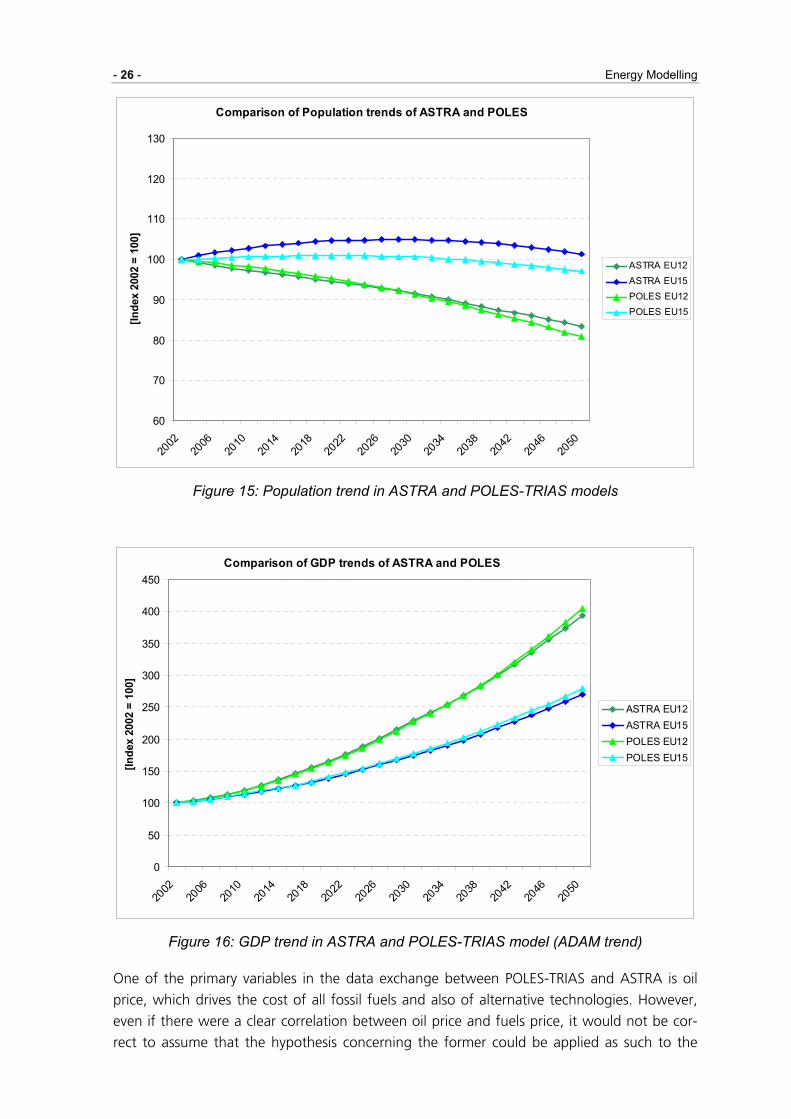
- 26 - Energy Modelling
Comparison of Population trends of ASTRA and POLES
60
70
80
90
100
110
120
130
2002
2006
2010
2014
2018
2022
2026
2030
2034
2038
2042
2046
2050
[Ind
ex 2
002
= 10
0]
ASTRA EU12ASTRA EU15POLES EU12POLES EU15
Figure 15: Population trend in ASTRA and POLES-TRIAS models
Comparison of GDP trends of ASTRA and POLES
0
50
100
150
200
250
300
350
400
450
2002
2006
2010
2014
2018
2022
2026
2030
2034
2038
2042
2046
2050
[Inde
x 20
02 =
100
]
ASTRA EU12ASTRA EU15POLES EU12POLES EU15
Figure 16: GDP trend in ASTRA and POLES-TRIAS model (ADAM trend)
One of the primary variables in the data exchange between POLES-TRIAS and ASTRA is oil
price, which drives the cost of all fossil fuels and also of alternative technologies. However,
even if there were a clear correlation between oil price and fuels price, it would not be cor-
rect to assume that the hypothesis concerning the former could be applied as such to the

TRIAS D3 Outlook for Global Transport and Energy Demand - 27 -
latter. Actually, historical trends show that fuel price is generally less volatile than oil price.
For instance, the crude oil price has grown by about 120% in the last 6 years (from an aver-
age of 16.5 $/Barrel in 1999 to an average of 37.5 $/Barrel in 2004), while gasoline price in
the same period has grown significantly less (e.g. of about 35% in Italy, of about 40% in
Germany, etc.).
It was the energy market POLES-TRIAS model, which took care of the simulation of the fuels
price development as a consequence of the oil price hypothesis assumed in the scenarios.
And since one crucial variable affecting the development of fuels price is transport demand,
this was provided to POLES-TRIAS form the ASTRA model. Transport demand affects prices
but also the reverse is true, so there is a feedback relation to take into account. For that rea-
son, the interactions between POLES-TRIAS and ASTRA for simulating the scenarios has been
obtained working interactively with the models in a feedback process.
Taking transport cost, as generalised costs, and transport demand, as vehicles-kms, from the
ASTRA model, POLES-TRIAS has computed the fleet evolution and fuels price development. In
turn, the fuels (resource) price forecast by POLES-TRIAS has been used in ASTRA to revise the
transport demand forecast, which is again fed into POLES.
The loop transport demand – fuels price impact – impact on transport demand – impact on
fuels price between the three models has requested several iterations (Figure 17) before
reaching the equilibrium. The calculation of the baseline was started by ASTRA passing its
relevant data to POLES, which then handed over its results to the BIOFUEL model. From both
models, results were given back to ASTRA where the next step was started. For all nine sce-
narios POLES-TRIAS started the calculation, giving results to the BIOFUEL model and ASTRA,
and BIOFUEL gave its results to ASTRA as well. ASTRA started the baseline calculation be-
cause it calculated the GDP needed by POLES. On the other hand, POLES-TRIAS started the
scenario calculations based on the final ASTRA baseline results because in POLES-TRIAS and
BIOFUEL, the politic measures were implemented. These were carbon tax levels and subsidies
for new fuel technologies. Figure 17 summarises which variables are exchanged and how
ASTRA, POLES-TRIAS and BIOFUEL are linked.
GDP
Fuel demand
Fossil Fuel Prices
Subsidies
Biofuel Fuel Prices
Investment
Fossil Fuel Trade
Carbon Taxes
ASTRA
POLES BIOFUELFossil Fuel Prices
Subsidies
Investment
Carbon Taxes
GDP
Fuel demand
Base
line
3
1 2Scenarios
1
2 3
Figure 17: Data exchange between ASTRA, POLES-TRIAS and BIOFUEL models

- 28 - Economic, Transport and Environmental Modelling
4 Economic, Transport and Environmental Modelling
This section describes the three models used in TRIAS to analyse the transport system, the
environmental impacts of transport and the economic impacts of the scenarios and policies
tested in TRIAS. The three models include VACLAV, Regio-SUSTAIN and ASTRA. VACLAV is a
transport network model covering the whole EU as well as the relevant long distance trans-
port modes: road, rail, inland waterway, shipping and air transport. Regio-SUSTAIN enables
to calculate immission concentrations on a local scale such that the model in TRIAS will be
applied for two selected regions of Europe. ASTRA is an integrated transport – economy -
environment model, which in TRIAS in particular is used to estimate the indirect economic
impacts of transport and energy policies. The three models, their improvements and their
application are explained in the following sections.
4.1 The ASTRA Model
ASTRA stands for Assessment of Transport Strategies. The model is developed since 1997
with the purpose of strategic assessment of policies in an integrated way i.e. by considering
the feedback loops between the transport system and the economic system. The most de-
tailed description of ASTRA is provided by Schade (2005). The following sections give an
overview on ASTRA taking into account extensions made for the TRIAS project.
The most important as well as resource consuming improvement, though not visible in the
technical capabilities of ASTRA, is the fact that ASTRA is physically modularised in TRIAS. So
far, ASTRA was only conceptually modularised, which means that all former modules of
ASTRA were implemented within one physical software file. In TRIAS physical modularisation
is implemented, which required both software reengineering of the existing modules and the
development of a software that links separate ASTRA modules into one software file again,
because the applied Vensim System Dynamics software is working only with one physical file.
The big advantage of modularisation justifying the efforts is that a physically modularised
ASTRA can be developed further applying the knowledge and organisation processes of pro-
fessional distributed software development i.e. the separate modules can be improved and
tested separately by independent developer teams and a repository supports version control-
ling and change management of the ASTRA modules.
4.1.1 Description of ASTRA
This section provides a description of the ASTRA model starting with the basic modelling
concept and an overview of the whole model framework. The overview is followed by a de-
scription of important feedback loops of the full model and two sections describing the clas-
sification structures of ASTRA: spatial differentiation and sectoral classification.

TRIAS D3 Outlook for Global Transport and Energy Demand - 29 -
Concept of ASTRA
The approach for the original development of ASTRA was to build an integrative coded
model that is implemented with the System Dynamics standard software Vensim. If available
ASTRA draws on existing models of different scientific disciplines. Otherwise models are
newly developed. Core models that spin off for ASTRA are the European transport model
STREAMS and its updated version SCENES (ME&P 2000), the macroeconomic system dynam-
ics model ESCOT (SCHADE/ROTHENGATTER/SCHADE 2002) and a set of environmental models
that have been developed for purposes of Strategic Environmental Assessment (SEA) of the
German federal cross-modal transport infrastructure plan (BVWP) (IWW et al. 1998,
GÜHNEMANN 2000). Major completions and extensions of ASTRA have been achieved in the
TIPMAC project and the related dissertation of Wolfgang Schade, which constituted so far
the most comprehensive description of ASTRA (SCHADE 2005).
From each of the three above models the major feedback loops were analysed and selected
for implementation in ASTRA. Since two out of the three models were not developed with
System Dynamics this required reformulation and adaptation of their equations such that the
final outcome looked rather different to the originating model. But the spirit of the identified
feedbacks was maintained. One reason why system dynamics was chosen as methodology is
founded in the flexibility to incorporate elements of different modelling approaches. In that
sense, to model ASTRA various techniques from other modelling approaches outside system
dynamics are borrowed. This includes econometrics to estimate functional relationships be-
tween variables for which all relevant data is available. It incorporates input-output analysis to
reflect sectoral relationships of economies. It even covers equilibrium approaches as these are
frequently used in transport modelling. Obviously these have to be adapted as in some cases
there are fundamental differences in approaches e.g. an equilibrium concept in its pure form
is diametrically opposed to the approach of system dynamics that can be called a disequilib-
rium approach from the viewpoint of neo-classical economics.
Finally, the problems of analysing and visualising the model are of key importance to build, to
communicate and to control large-scale models. In this respect system dynamics and its tools
offer powerful capabilities that are intensively used for verification and validation of ASTRA.
Overview on ASTRA
The ASTRA model consists of nine modules that are all implemented within one Vensim sys-
tem dynamics software file. One scenario simulation between 1990 and 2050 with 2-yearly
saving intervals of the selected result indicators generates about 800 Mega-Byte of output
data for the EU29 countries. The model comprises close to 30 million objects in Vensim. Ob-
jects could be variables, which is equal to equations, constants or data input. More than 1
million objects are level variables and hence are dynamic variables. Two major types of level
variables can be distinguished: delay variables and accumulating variables of which the for-
mer stand for the greater share of level variables in the model. About 12.000 time series are
used to calibrate ASTRA for the period 1990 until 2000. Variables are grouped into the fol-
lowing nine modules:
• Population module (POP),

- 30 - Economic, Transport and Environmental Modelling
• Macro-economic module (MAC),
• Regional economic module (REM),
• Foreign trade module (FOT),
• Infrastructure module (INF),
• Transport module (TRA),
• Environment module (ENV),
• Vehicle fleet module (VFT) and
• Welfare measurement module (WEM).
An overview on the nine modules and their main interfaces is presented in Figure 18. The
aggregate level of the figure provides the only exhaustive presentation of ASTRA. Going to
one further level of detail with the description would already be outside what could be pre-
sented within one figure or one comprehensive set of equations. To cope with this difficulty
the following explanations are zooming top-down into the details of the model necessarily
having some overlap in the descriptions from the upper levels to the more detailed levels to
pick-up the thread at each level of description again.
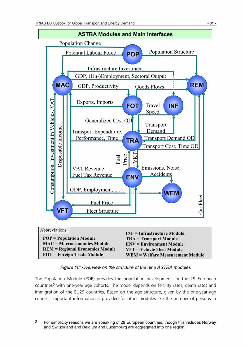
TRIAS D3 Outlook for Global Transport and Energy Demand - 31 -
POP
MAC
FOT
REM
TRA
WEM
ENV
VFT
Potential Labour Force Population Structure D
ispos
able
Inco
me
Con
sum
ptio
n, In
vest
men
t in
Veh
icle
s, V
AT
GDP, (Un-)Employment, Sectoral Output
Population Change
VK
T
Goods Flows
Car
Fle
et
Fuel Price
GDP, Productivity
Exports, Imports
Transport Expenditure, Performance, Time
VAT Revenue Fuel Tax Revenue
GDP, Employment, ....
Fuel
Pr
ice
Emissions, Noise, Accidents
Transport Cost, Time OD Transport Demand OD
POP = Population Module MAC = Macroeconomics Module REM = Regional Economics Module FOT = Foreign Trade Module
Abbreviations: INF = Infrastructure Module TRA = Transport Module ENV = Environment Module VFT = Vehicle Fleet Module WEM = Welfare Measurement Module
ASTRA Modules and Main Interfaces
Generalized Cost OD
Fleet Structure
INF
Infrastructure Investment
TransportDemand
Travel Speed
Figure 18: Overview on the structure of the nine ASTRA modules
The Population Module (POP) provides the population development for the 29 European
countries2 with one-year age cohorts. The model depends on fertility rates, death rates and
immigration of the EU29 countries. Based on the age structure, given by the one-year-age
cohorts, important information is provided for other modules like the number of persons in
2 For simplicity reasons we are speaking of 29 European countries, though this includes Norway
and Switzerland and Belgium and Luxemburg are aggregated into one region.

- 32 - Economic, Transport and Environmental Modelling
the working age or the number of persons in age classes that permit to acquire a driving li-
cence. POP is calibrated to EUROSTAT population predictions.
The MAC provides the national economic framework, which imbeds the other modules. The
MAC could not be categorised explicitly into one economic category of models for instance a
neo-classical model. Instead it incorporates neo-classical elements like production functions.
Keynesian elements are considered like the dependency of investments on consumption,
which are extended by some further influences on investments like exports or government
debt. Further elements of endogenous growth theory are incorporated like the implementa-
tion of endogenous technical progress (e.g. depending on sectoral investment) as one impor-
tant driver for the overall economic development.
Six major elements constitute the functionality of the macroeconomics module. The first is
the sectoral interchange model that reflects the economic interactions between 25 economic
sectors of the national economies. Demand-supply interactions are considered by the second
and third element. The second element, the demand side model depicts the four major com-
ponents of final demand: consumption, investments, exports-imports and the government
consumption. The supply side model reflects influences of three production factors: capital
stock, labour and natural resources as well as the influence of technological progress that is
modelled as total factor productivity. Endogenised total factor productivity depends on in-
vestments, freight transport times and labour productivity changes. The fourth element of
MAC is constituted by the employment model that is based on value-added as output from
input-output table calculations and labour productivity. Employment is differentiated into
full-time equivalent employment and total employment to be able to reflect the growing im-
portance of part-time employment. In combination with the population module unemploy-
ment was estimated. The fifth element of MAC describes government behaviour. As far as
possible government revenues and expenditures are differentiated into categories that can be
modelled endogenously by ASTRA and one category covering other revenues or other ex-
penditures. Categories that are endogenised comprise VAT and fuel tax revenues, direct
taxes, import taxes, social contributions and revenues of transport charges on the revenue
side as well as unemployment payments, transfers to retired and children, transport invest-
ments, interest payments for government debt and government consumption on the expen-
diture side.
Sixth and final of the elements constituting the MAC are the micro-macro bridges. These link
micro- and meso-level models, for instance the transport module or the vehicle fleet module
to components of the macroeconomics module. That means, that expenditures for bus trans-
port or rail transport of one origin-destination pair (OD) become part of final demand of the
economic sector for inland transport within the sectoral interchange model. The macroeco-
nomics module provides several important outputs to other modules. The most important
one is, for sure, Gross Domestic Product (GDP). This is for instance required to calculate sec-
toral trade flows between the European countries. Other examples are employment and un-
employment representing two influencing factors for passenger transport generation. Sec-
toral production value is driving national freight transport generation. Disposable income
exerting a major influence on car purchase affecting finally the vehicle fleet module and even
passenger transport emissions.

TRIAS D3 Outlook for Global Transport and Energy Demand - 33 -
The Regional Economic Module (REM) mainly calculates the generation and spatial distribu-
tion of freight transport volume and passenger trips. The number of passenger trips is driven
by employment situation, car-ownership development and number of people in different age
classes. Trip generation is performed individually for each of the 71 zones of the ASTRA
model. Distribution splits trips of each zone into three distance categories of trips within the
zone and two distance categories crossing the zonal borders and generating OD-trip matrices
with 71x71 elements for three trip purposes. Freight transport is driven by two mechanisms:
Firstly, national transport depends on sectoral production value of the 15 goods producing
sectors where the monetary output of the input-output table calculations are transferred into
volume of tons by means of value-to-volume ratios. For freight distribution and the further
calculations in the transport module the 15 goods sectors are aggregated into three goods
categories. Secondly, international freight transport i.e. freight transport flows that are cross-
ing national borders are generated from monetary Intra-European trade flows of the 15
goods producing sectors. Again transfer into volume of tons is performed by applying value-
to-volume ratios that are different from the ones applied for national transport. In that sense
the export model provides generation and distribution of international transport flows within
one step on the base of monetary flows.
The Foreign Trade Module (FOT) is divided into two parts: trade between the EU29 European
countries (INTRA-EU model) and trade between the EU29 European countries and the rest-of-
the world (RoW) that is divided into nine regions (EU-RoW model with Oceania, China, East
Asia, India, Japan, Latin America, North America, Turkey, Rest-of-the-World). Both models
are differentiated into bilateral relationships by country pair by sector. The INTRA-EU trade
model depends on three endogenous and one exogenous factor. World GDP growth exerts
an exogenous influence on trade. Endogenous influences are provided by GDP growth of the
importing country of each country pair relation, by relative change of sectoral labour produc-
tivity between the countries and by averaged generalised cost of passenger and freight trans-
port between the countries. The latter is chosen to represent an accessibility indicator for
transport between the countries. The EU-RoW trade model is mainly driven by relative pro-
ductivity between the European countries and the rest-of-the-world regions. Productivity
changes together with GDP growth of the importing RoW-country and world GDP growth
drive the export-import relationships between the countries. Since, transport cost and time
are not modelled for transport relations outside EU29 transport is not considered in the EU-
RoW model. The resulting sectoral export-import flows of the two trade models are fed back
into the macroeconomics module as part of final demand and national final use respectively.
Secondly, the INTRA-EU model provides the input for international freight generation and
distribution within the REM module.
The Infrastructure Module (INF) provides the network capacity for the different transport
modes. Infrastructure investments derived both from the economic development provided by
the MAC and from infrastructure investment policies alter the infrastructure capacity. Using
speed flow curves for the different infrastructure types and aggregate transport demand the
changes of average travel speeds over time are estimated and transferred to the TRA where
they affect the modal choice.
The major input of the Transport Module (TRA) constitutes the demand for passenger and
freight transport that is provided by the REM in form of OD-matrices. Using transport cost

- 34 - Economic, Transport and Environmental Modelling
and transport time matrices the transport module performs the modal-split for five passenger
modes and three freight modes. The cost and time matrices depend on influencing factors
like infrastructure capacity and travel speeds both coming from the INF module, structure of
vehicle fleets, transport charges, fuel price or fuel tax changes. Depending on the modal
choices, transport expenditures are calculated and provided to the macroeconomics module.
Changes in transport times are also transferred to the macroeconomics module such that
they can influence total factor productivity. Considering load factors and occupancy rates
respectively, vehicle-km are calculated.
Major outputs of the TRA provided to the Environment Module (ENV) are the vehicle-
kilometres-travelled (VKT) per mode and per distance band and traffic situation respectively.
Based on these traffic flows and the information from the vehicle fleet model on the national
composition of the vehicle fleets and hence on the emission factors, the environmental mod-
ule calculates the emissions from transport. Besides emissions, fuel consumption and, based
on this, fuel tax revenues from transport are estimated by the ENV. Traffic flows and accident
rates for each mode form the input to calculate the number of accidents in the European
countries. Expenditures for fuel, revenues from fuel taxes and value-added-tax (VAT) on fuel
consumption are transferred to the macroeconomics module and provide input to the eco-
nomic sectors producing fuel products and to the government model.
The Vehicle Fleet Module (VFT) describes the vehicle fleet composition for all road modes.
Vehicle fleets are differentiated into different age classes based on one-year-age cohorts and
into different emission standard categories. The car vehicle fleet is developing according to
income changes, development of population, fuel prices, fuel taxes, maintenance and pur-
chase cost of vehicles, mileage and the density of filling stations for the different type of fu-
els. Vehicle fleet composition of buses, light-duty vehicles and heavy-duty vehicles mainly
depends on travelled kilometres and the development of average annual mileages per vehicle
of these modes. The purchase of vehicles is translated into value terms and forms an input of
the economic sectors in the MAC that cover the vehicle production.
Finally, in the Welfare Measurement Module (WEM) major macro-economic, environmental
and social indicators can be compared and analysed. Also different assessment schemes that
combine indicators into aggregated welfare indicators for instance an investment multiplier
are provided in the WEM. In some cases, e.g. to undertake a CBA, the functionality is sepa-
rated into further tools to avoid excessive growth of the core ASTRA model by including the
assessment scheme directly within the model.
Important Feedback Loops of ASTRA
The feedback loop concept constitutes the most important concept of system dynamics,
which is the underlying modelling methodology of ASTRA. Starting from a causal analysis
structured by the relations of the system to be modelled a feedback structure inherent to the
system is developed. A feedback loop is identified when a sequence of relations of which the
first relation commenced at the system component X reaches the component X again. Usu-
ally the sequence of relations leading from X via other system components back to X again
incorporates a time structure i.e. commencing at X and feeding back to X would not happen
at the same point of time. In fact, feedback loops are the most important structures of com-

TRIAS D3 Outlook for Global Transport and Energy Demand - 35 -
plex systems. STERMAN (2000 p.13) puts it this way: "All systems, no matter how complex, consist of networks of positive and negative feedbacks, and all dynamics arise from the inter-
action of these loops with one another."
Feedback loops can be distinguished into two categories: negative feedback loops and posi-
tive feedback loops (Bossel 1994, Sterman 2000):
• Negative feedback loops are target-seeking. They tend to counteract any disturbance
and lead systems towards a stable state. Control of the temperature in a room with a
thermostat constitutes one example of a negative feedback loop. If temperature dif-
fers from the envisaged temperature (= target), heating will be activated until the dif-
ference between actual and envisaged temperature approaches zero.
• Positive feedback loops are present if the change of a system component leads to
changes in other components that finally strengthen the original process. Positive
feedback introduces an accelerating process of growth or decline. A system consisting
only of positive feedbacks tends to explode or to implode. The well-known stylised
fact of dependency between wages and prices provides an example for a positive
feedback. Higher wages lead to inflation. Inflation leads to higher prices and higher
prices result in claims for higher wages such that the inflation-spiral moves. This ex-
ample reveals that positive does not at all mean favourable in connection with feed-
back loops.
Since, analysis of the feedback loops of a system enable to describe and understand the func-
tionality of a system it is used in the following to deepen the explanation of ASTRA. Seven of
the most relevant feedback loops are presented by causal loop diagrams. The diagrams cover:
• Consumption feedback loop,
• Investment feedback loop,
• Employment feedback loop,
• Government feedback loop,
• Export feedback loop,
• Freight transport feedback loop and
• Passenger transport feedback loop.
However, it remains impossible to present all influences affecting each loop such that in
some cases interactions e.g. between the different feedback loops are explained in the text
or in further literature (SCHADE 2005).
First, the consumption feedback loop is presented in Figure 19. The basic loop presents a
positive feedback such that growth in consumption is generating growth in GDP and income
leading to further growth in consumption in the next time period. However, negative influ-
ences from other parts of the model could break the inherent growth tendency of this loop.
These could either stem from decreases of other elements of final demand, e.g. reduced in-
vestment, government consumption or exports (circle 1), or from the combined influences of
sectoral shifts induced by changes in the transport system (circle 2) and the tax system (circle
3). The former would shift private consumption expenditures between sectors and could

- 36 - Economic, Transport and Environmental Modelling
shrink consumption because of tax differentials between transport consumption and non-
transport consumption while the latter would reduce disposable income available for con-
sumption decreasing finally the consumption expenditures.
Sector Energy
Fuel consumption / ENV
Sector Vehicles
Car purchase / VFT
Sector Transport air maritime
Demand transport services / TRA
Sector Transport inland
Consumption per sector
Consumption transport total
Change transport consumption
Final demand
Consumption non-transport sectors
Government / MAC
Export / FOT
Investment / MAC
Import / FOT
GDP National income
National consumption
Disposable income
Depreciation / MAC
Non-national consumption
Savings
Direct tax
Indirect tax revenue VAT revenue
Fuel consumption / ENV
Fuel tax revenue VAT from fuel
Transfers to households
Sectoral split consumption +
Transport charge /TRA +
2
3
1
+
+
+ +
+ +
+
+
+
+ + + + +
+ + + + -
+ + +
+
+
+
+
+
+
- - - +
+ +
+
+ +
-
Figure 19: The consumption feedback loop in ASTRA and its impacts from transport
Investments are also affected by a major positive loop as investment increase capital stock
and total factor productivity (TFP) of an economy leading to growing potential output and
GDP that drives income and consumption feeding back to an increase of investments (Figure
20). However, this loop could also be influenced by other interfering loops that would break
the growth tendency. Increasing government debt could lead to crowding out tendencies
that provide a negative impact on investment (circle 1). Exports e.g. influenced by growing
transport cost could decrease reducing investments (circle 2). Changes in transport demand
e.g. modal-shifts due to policies that would shift demand from modes with high investment
needs to modes with low investment needs per unit of demand would reduce investments
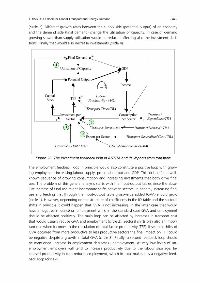
TRIAS D3 Outlook for Global Transport and Energy Demand - 37 -
(circle 3). Different growth rates between the supply side (potential output) of an economy
and the demand side (final demand) change the utilisation of capacity. In case of demand
growing slower than supply utilisation would be reduced affecting also the investment deci-
sions. Finally that would also decrease investments (circle 4).
Final Demand
Utilisation of Capacity
Potential Output
TFP
GDP
Income
Capital Stock
Labour Productivity / MAC
Transport Times/TRA
Consumption per Sector
Transport Expenditure/TRA
Investment per Sector
Export per Sector
Goverment Debt / MAC
Transport Generalised Cost / TRA
+
+
+
+ +
- +
+
+
+
+ +
+ -
+ -
-
+
+
+
GDP of other countries/MAC +
+
1
4
2
Transport Investment Transport Demand / TRA+
+ 3
Figure 20: The investment feedback loop in ASTRA and its impacts from transport
The employment feedback loop in principle would also constitute a positive loop with grow-
ing employment increasing labour supply, potential output and GDP. This kicks-off the well-
known sequence of growing consumption and increasing investments that both drive final
use. The problem of this general analysis starts with the input-output tables since the abso-
lute increase of final use might incorporate shifts between sectors. In general, increasing final
use and feeding that through the input-output table gross-value added (GVA) should grow
(circle 1). However, depending on the structure of coefficients in the IO-table and the sectoral
shifts in principle it could happen that GVA is not increasing. In the latter case that would
have a negative influence on employment while in the standard case GVA and employment
should be affected positively. The main loop can be affected by increases in transport cost
that would usually reduce GVA and employment (circle 2). Sectoral shifts play also an impor-
tant role when it comes to the calculation of total factor productivity (TFP). If sectoral shifts of
GVA occurred from more productive to less productive sectors the final impact on TFP could
be negative despite a growth in total GVA (circle 3). Finally, a second feedback loop should
be mentioned. Increase in employment decreases unemployment. At very low levels of un-
employment employers will tend to increase productivity due to the labour shortage. In-
creased productivity in turn reduces employment, which in total makes this a negative feed-
back loop (circle 4).

- 38 - Economic, Transport and Environmental Modelling
Investment per Sector
Consumption per Sector
Transport Expenditures / TRA Final Use per Sector
Government Consumption / MAC
Export per Sector
Transport Generalised Cost / TRA
GDP
Potential Output
Input-Output Table Transport Cost / TRA
Labour Supply
Employment per Sector Gross-Value-Added per Sector
Unemployment Labour Productivity per Sector TFP
Active Labour Force Population / POP
+
+ -
+ + + +/-
+
+
+ +
+
- -
+
+
(+)
(+)
- +
+ +
-
(+)
2
+
3
(+) - 4
1
Final Demand Import per Sector / - + +
Utilisation of Capacity -
+ Yearly working time
+
Figure 21: The employment feedback loop in ASTRA and its impacts from transport
The government feedback loop seems to be most difficult to describe since the government
experiences many influences as the large number of influencing arrows to government reve-
nues (circle 1) and government expenditures (circle 2) reveal. However, the impacts it exerts
are mainly all policy measures e.g. adjusting its expenditure level by adapting the transfers to
retired, children or unemployed. To adjust these automatically, e.g. in case of negative
budget balance and high government debt, would be an option to close feedback loops.
Experimental versions of these feedbacks are implemented in ASTRA but with the argument
that these are all policy measures outside transport policy they are not used such that the
only feedback remains the negative impact of high government debt on investment deci-
sions. A reduction of government debt would increase investments in case crowding out pre-
vailed leading to higher GDP and consumption. This would exert a positive impact on reve-
nues from direct and indirect taxes leading to growth of government revenues and a more
positive government balance, which in turn would reduce government debt. And that is
where we commenced the loop such that this also constitutes a positive i.e. reinforcing loop.
Another important loop is the one e.g. the German government struggles with. Starting with
a high government debt large interest payments are payable leading to increased govern-
ment expenditures and a potentially negative budget balance that in turn increases the debt.
Again this constitutes a positive feedback loop as it reinforces the original stimulus (circle 3).

TRIAS D3 Outlook for Global Transport and Energy Demand - 39 -
Final Demand per Sector GDP
Consumption IO-Table
GVA
Investment per Sector
VAT
Indirect Taxes
Fuel Consumption / ENV
Fuel Tax
Imports / MAC
Imports TaxEmploymentUnemployment
Government Consumption
Social Contributions
Government Revenues
Transport Charges / TRA
Direct Taxes
Other Revenues
Population / POP
Transfers to Children
Transfers to Retired
Transfers to Unemployed
Government Balance
Government Expenditures
Government Investment
Government Debt
Interest Payment
Long-term Interest Rate / MAC
Transport Infrastructure Investment
Infrastructure Policy
+
+ +
+
+
+ +
+
+
+
+
+ ++
+
+
+ +
+/-
+/-
+ + + +
+ +
+ +/-
+
+
+
-
+
-
-
+ + ++
+
+
+
+
3
-
+2 1
Figure 22: The government feedback loop in ASTRA and its impacts from transport
The export loop in Figure 23 resembles very much the Heckscher-Ohlin model of trade be-
tween two countries (HECKSCHER 1919). Country A is importing goods from country B, which
appear as exports on the demand side of country B and increase GDP of B. Hence, country B
increases imports, which in turn leads to growing exports of country A finally increasing the
GDP of country A. The basic loop is reinforcing. However, one of its major influences is con-
stituted by sectoral relative labour productivity between the two countries (circle 1). If country
A becomes more productive than B it will increase its exports to B and vice versa, while B will
loose exports such that the loop set-up by mutual growth of GDP could be broken by re-
duced GDP of country B. This impact could be different for any of the 25 sectors of ASTRA.
A further influence on exports stems from transport. The quality of transport connections
between countries A and B can be expressed by the generalised cost of transport, which are
an aggregate of transport cost and monetised travel time as transport decisions not only de-
pend on cost but also on time conditions (ORTUZAR/WILLUMSEN 1998)3. Increased generalised
cost would then shrink exports or at least lower export growth, which in turn leads to declin-
ing imports probably in both countries (circle 2). Figure 23 indicates merely an influence from
3 In fact, further relevant conditions might exist e.g. reliability of transport, safety requirements.
But these could not be reflected in ASTRA, yet.

- 40 - Economic, Transport and Environmental Modelling
freight transport, but also changes of passenger transport could affect trade flows, consider-
ing exports of service sectors like tourism as part of the catering sector in ASTRA or the trans-
port service sectors themselves.
Transport Generalised Cost Transport Times Freight Transport
Import per Sector / A Export per Sector / B
Productivity per Sector / B
Relative Productivity A to B
GDP country A GDP country B
Productivity per Sector / A
Import other Countries / FOT
Export per Sector / A Import per Sector / B
Freight Transport Transport Times Transport Generalised Cost
Import other Countries / FOT
+ +
+
+
+
+ -
+/- +
+ +
+
+/- +
-
+ + +
+ +
+
1
-
- 2
2
Transport Cost / TRA +
Transport Cost / TRA +
Figure 23: The export feedback loop in ASTRA and its impacts from transport
The most obvious feedback loop of freight transport starting at freight modal-split includes
investments per sector that increase final use and output per sector (Figure 24). Domestic
output per sector drives the freight volume that does not cross the national border while the
trade flows generate the freight volume that crosses national borders. Freight flows are dis-
tributed onto the 71 potential destination zones though in this case not all destinations will
increase their flows in the same shares due to the difference in generalised cost changes and
transport characteristics. Finally, freight modal-split is performed but again increased demand
on a selected origin-destination (OD) pair is not spread evenly on the different modes and the
loop is closed by demand per mode. Additional to the direct link from final use to output per
sector there is the link via the input-output table where output of intermediates per sector is
calculated and then forms part of total output per sector (circle 1). In principle, this first feed-
back loop is positive though results depend to some extent on the structure of the modal-
shifts that might strengthen a mode with lower investment needs such that the loop could
then be reversed.
The second loop again starts at freight modal-split but is then continued via changes in
freight transport times that in general tend to increase with increasing demand for a mode,
though this should not necessarily be the case e.g. if economies of scale generate time sav-
ings in the logistic chain. Increasing transport times exert a negative impact on total factor

TRIAS D3 Outlook for Global Transport and Energy Demand - 41 -
productivity (TFP) arguing that freight transport constitutes an important element of today's
production processes (circle 2). Decreasing TFP slows down growth of GDP and consumption
leading to reduced final use. The remainder of this loop looks the same as for the previous
loop but opposite to that loop this freight-times-TFP loop belongs to the negative or damp-
ening category. Finally, one should also have in mind that passenger transport is interfering
with this loop as it also may influence freight transport times due to the usage of the same
transport network e.g. for cars and trucks (circle 3).
A further loop to mention accounts for the interaction between modal-split decisions and
destination choice, which is indicated by the circles number 4. As already discussed modal-
choice affects the freight transport times, but aggregate transport times for all modes serving
an OD-pair influence the destination choice. Altered destination choice again leads to a new
situation for modal-split and the loop commences again. However, these modal-choice and
destination choice decisions work on different time scales where modal-choice can be an
immediate or very short-run decision while destination choice would be affective on medium
term e.g. as it depends on setting-up new trade contacts or new business locations.
Government Consumption / MAC
Final Use per Sector
Consumption
GDP
TFP
Export per Sector
Export Flows OD per Sector
GDP / MAC
Productivity / MAC
Output per Sector
Output of Intermediates
Freight Transport Volume
Value-to Volume Ratio / REM
Freight Distribution
Freight Generalised Cost OD
Freight Cost / TRAIO-Table
GVA Transport Charge / TRA
Fuel Tax / ENV
Freight Modal / Split
Freight Times
Demand per Mode
Passenger Modal-Split / TRA Network Capacity / TRA
Investment per Sector
Export / FOT
Consumption / MAC
+
-
++
+
+
+ +- + +
++
+ +-
-
+
+ -
-
+
(+)++
+
+
+
++
+ +
-
+
-
+
+
+
+
+1
+
2
4
-
-
4
3
Figure 24: The freight transport feedback loops in ASTRA
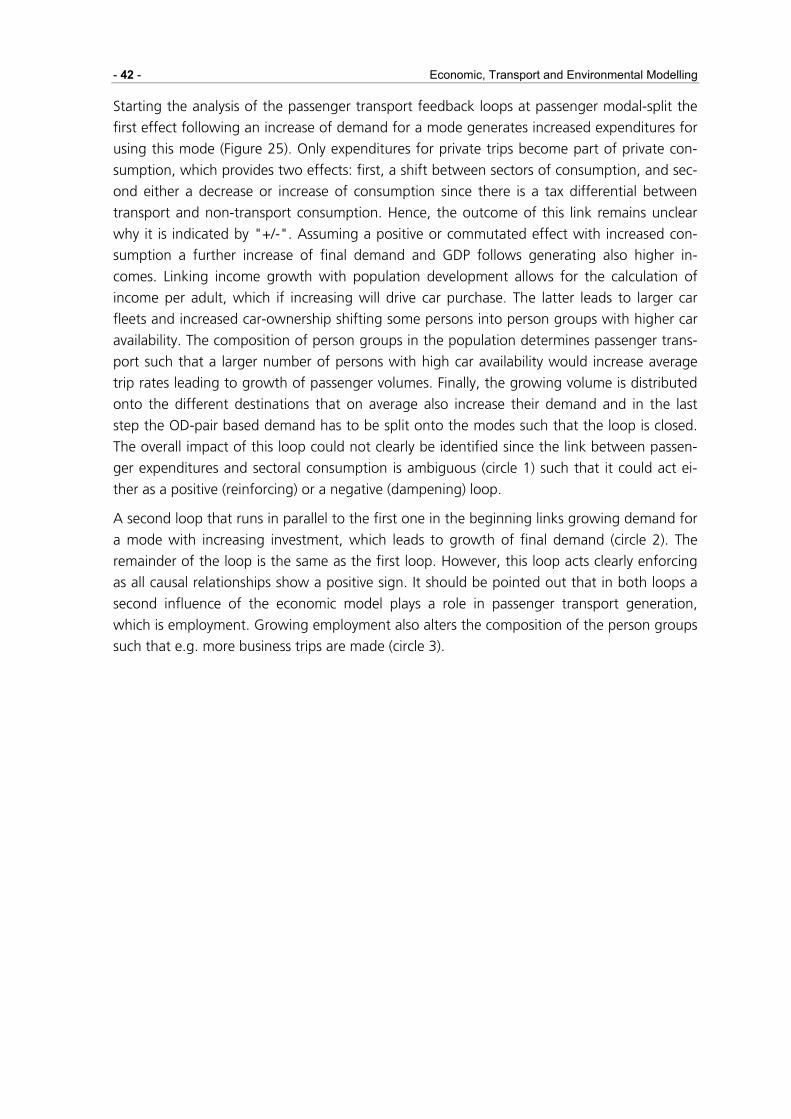
- 42 - Economic, Transport and Environmental Modelling
Starting the analysis of the passenger transport feedback loops at passenger modal-split the
first effect following an increase of demand for a mode generates increased expenditures for
using this mode (Figure 25). Only expenditures for private trips become part of private con-
sumption, which provides two effects: first, a shift between sectors of consumption, and sec-
ond either a decrease or increase of consumption since there is a tax differential between
transport and non-transport consumption. Hence, the outcome of this link remains unclear
why it is indicated by "+/-". Assuming a positive or commutated effect with increased con-
sumption a further increase of final demand and GDP follows generating also higher in-
comes. Linking income growth with population development allows for the calculation of
income per adult, which if increasing will drive car purchase. The latter leads to larger car
fleets and increased car-ownership shifting some persons into person groups with higher car
availability. The composition of person groups in the population determines passenger trans-
port such that a larger number of persons with high car availability would increase average
trip rates leading to growth of passenger volumes. Finally, the growing volume is distributed
onto the different destinations that on average also increase their demand and in the last
step the OD-pair based demand has to be split onto the modes such that the loop is closed.
The overall impact of this loop could not clearly be identified since the link between passen-
ger expenditures and sectoral consumption is ambiguous (circle 1) such that it could act ei-
ther as a positive (reinforcing) or a negative (dampening) loop.
A second loop that runs in parallel to the first one in the beginning links growing demand for
a mode with increasing investment, which leads to growth of final demand (circle 2). The
remainder of the loop is the same as the first loop. However, this loop acts clearly enforcing
as all causal relationships show a positive sign. It should be pointed out that in both loops a
second influence of the economic model plays a role in passenger transport generation,
which is employment. Growing employment also alters the composition of the person groups
such that e.g. more business trips are made (circle 3).
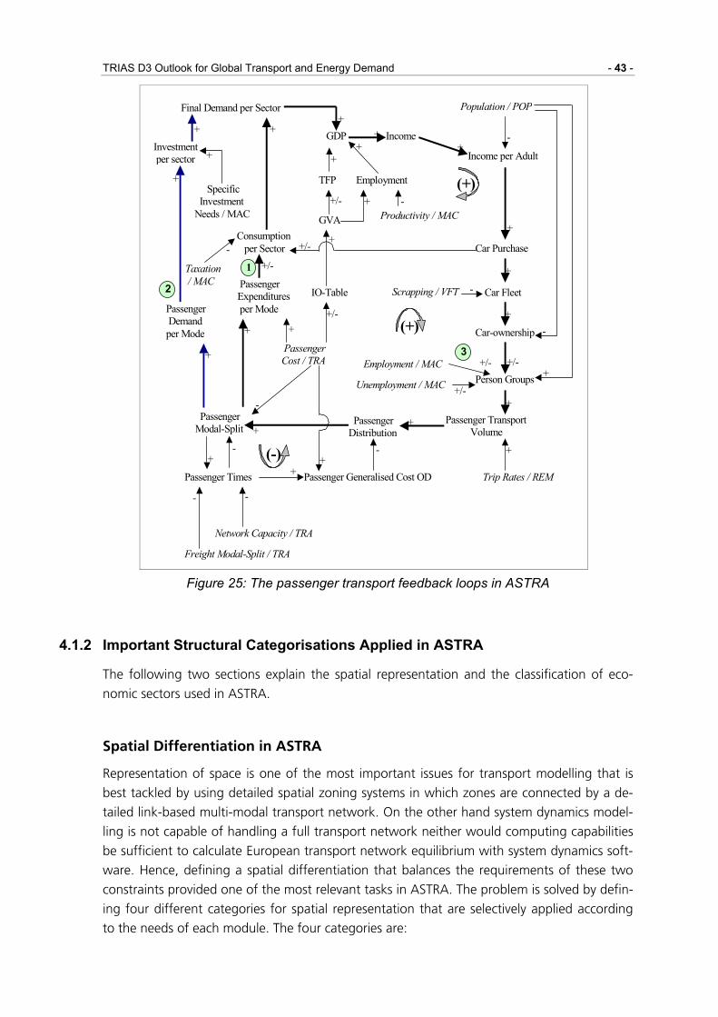
TRIAS D3 Outlook for Global Transport and Energy Demand - 43 -
Final Demand per Sector
GDP Income
Income per Adult
Population / POP
Employment
Productivity / MAC
TFP
GVA
Car Purchase
Car Fleet Scrapping / VFT
Car-ownership
Person Groups Employment / MAC
Unemployment / MAC
Passenger Transport Volume
Passenger Distribution
Trip Rates / REM
Consumption per Sector
IO-Table
Taxation / MAC Passenger
Expenditures per Mode
Passenger Cost / TRA
Investment per sector
Specific Investment Needs / MAC
Passenger Demand per Mode
Passenger Modal-Split
Passenger Times Passenger Generalised Cost OD
Freight Modal-Split / TRA
Network Capacity / TRA
+ + +
+ +
-
+
+
+
-
+
+
+ -
- -
-
+
+
-
+
+
+
+
+/-
+/- +/- +
- +
+
-
+ +/-
+/-
+/- +
+/-
+ +
+ -
(+)3
2
(+)
(-)
1
Figure 25: The passenger transport feedback loops in ASTRA
4.1.2 Important Structural Categorisations Applied in ASTRA
The following two sections explain the spatial representation and the classification of eco-
nomic sectors used in ASTRA.
Spatial Differentiation in ASTRA
Representation of space is one of the most important issues for transport modelling that is
best tackled by using detailed spatial zoning systems in which zones are connected by a de-
tailed link-based multi-modal transport network. On the other hand system dynamics model-
ling is not capable of handling a full transport network neither would computing capabilities
be sufficient to calculate European transport network equilibrium with system dynamics soft-
ware. Hence, defining a spatial differentiation that balances the requirements of these two
constraints provided one of the most relevant tasks in ASTRA. The problem is solved by defin-
ing four different categories for spatial representation that are selectively applied according
to the needs of each module. The four categories are:

- 44 - Economic, Transport and Environmental Modelling
• Countries: current EU27 member states plus Norway and Switzerland are treated
separately as countries with the exception of Belgium and Luxemburg that form one
region such that this category consists of 28 entities.
• Functional zones: the 271 NUTS II zones of the EU27+2 countries are grouped into
four different zone types per country for EU15 and two different zone types for the
other countries according to their population density and settlement patterns. As not
all zones exist in every country this amounts in total to 71 entities.
• Passenger distance bands: passenger transport originating in a certain zone is divided
into five different categories of trip distances. Trips belonging to the three shorter dis-
tance categories remain within the zone itself, while the two longer distance catego-
ries may both cross borders of the zone and borders of the countries.
• Freight distance bands: freight transport originating in a certain zone is divided into
four different categories of trip distances. Tons transported belonging to the shortest
distance category remain within the zone itself. Tons transported in the second dis-
tance category may cross borders of the zones but not of the country. Tons trans-
ported within the two longer distance categories may both cross borders of the zones
and borders of the countries.
The specific application of spatial categories in the nine modules of ASTRA is shown in Table
3.
Table 3: Summary of spatial categorisations used in different modules of ASTRA
Spatial category POP MAC FOT REM INF TRA VFT ENV WEM
Countries X X X X X X X X X
Functional zones (x) X X X (x) (x)
Passenger dis-tance bands
(x) X (X) X X
Freight distance bands
(x) X (X) X X
Legend: X = category fully applied in module; (x) = only limited use of category e.g. only within interface to module
Using the country level for the set-up of the top-level spatial category is obvious for two rea-
sons. Firstly, administrative and statistical structures are defined at least on the base of differ-
entiating countries such that to fulfil the needs of each model for input or calibration data
the country level remains most important. Additionally some data e.g. input-output tables are
only available on country level. Secondly, policy analysis on European scale requires the provi-
sion of conclusions at least on the distribution of policy impacts between the countries.
The second level of spatial categorisation results from a balanced judgement of factors like
data availability, transport model requirements, soft- and hardware capabilities. To a large
extent data differentiated into detailed spatial categories for all European countries is pro-
vided by EUROSTAT on NUTS II level, though availability on NUTS-III level from EUROSTAT or

TRIAS D3 Outlook for Global Transport and Energy Demand - 45 -
even on lower levels from national statistical offices is increasing. NUTS-II level consists of 271
zones for the EU27+2 countries. Using NUTS-II in a system dynamics model seems not to be
feasible due to combined soft- and hardware restrictions as already the OD-matrices would
have more than 70.000 elements, a number that would even increase when it comes to con-
sider different modes and trip purposes, also. Furthermore it is not the idea of system dynam-
ics to model every detail but to consider representative structures that shape the behaviour of
the system under analysis. Taking transport as the system requiring the most sophisticated
level of spatial differentiation in ASTRA a categorisation should be developed that reduces
the number of spatial entities by clustering NUTS-II zones into groups that are homogenous
with respect to their transport mechanisms. These groups of zones are called functional
zones. For the purpose of grouping zones population density and the relative position of a
zone within all zones of one country are selected as criteria. Firstly, population density seems
to be reasonable as it determines most relevant transport characteristics e.g. high density
zones can be expected to have competitive public transport by tram or metro, while low den-
sity areas are more bound to car usage. On average train connections between two high
density areas should be better than between two lower density areas and so on. It seems that
a differentiation into four functional zones would provide the minimum required information
to cope with the needs of transport modelling. Hence, the following categorisation of func-
tional zones is set-up listed in order of decreasing population density:
• Metropolitan Areas (MPA);
• High Density Areas (HDA);
• Medium Density Areas (MDA);
• Low Density Areas (LDA).
Secondly, taking population density as the only and the same criteria for all countries would
lead to some countries that would show representatives only in one or two of the categories
of zones, which means to loose potential differentiation as the matrices in ASTRA then would
include many empty cells. Hence, the relative position within a country determines the fur-
ther criteria for grouping zones such that e.g. for a country that would have exactly four
NUTS-II zones each zone would belong to a different category of functional zone and the
assignment would fit to a ranking of their zonal population densities.
Following these two criteria all EU15 countries besides Ireland and Denmark would show
representatives in all categories. In Ireland only three functional zones are present while in
Denmark only two are considered, leading in total to the number of 53 functional zones for
EU15. For the EU12 member states plus Norway and Switzerland a slightly different approach
was taken. The six smaller countries Slovenia, Malta, Cyprus, Estonia, Latvia and Lithuania
were not differentiated into zones at all due to their limited size. For the other countries al-
ways a split into two zones is applied using gdp/capita as the main criteria. This led to the
fact that always the capitals plus at maximum one further prosperous neighbouring zone
were grouped into the same zone (MPA) while the other zones were grouped into the other
zone (MDA).
The classification of NUTS-II zones into the functional zones of the ASTRA model is obtained
following population density data and gdp per capita data of NUTS-II zones drawn from the

- 46 - Economic, Transport and Environmental Modelling
SCENES database (SCENES 2000) or the EUROSTAT Yearbook of Regions (EUROSTAT 2002).
Considering in countries with large numbers of zones that the medium density areas are well
represented the categorisation of NUTS-II zones leads to the structure of functional zones
presented in Table 4. The table shows for the EU15 countries the thresholds used to define
functional zones per country. Population density is expressed in persons per square km and
GDP per capita in EURO/1999 per inhabitant per year.

TRIAS D3 Outlook for Global Transport and Energy Demand - 47 -
Table 4: Summary of categorisation of NUTS II zones into functional zones in ASTRA for EU27+2
Type of Zone Metropolitan Ar-eas (MPA)
High Density Ar-eas (HDA)
Medium Density Areas (MDA)
Low Density Areas (LDA)
Country Population
density # Population
density # Population
density # Population
density #
EU15 countries Austria > 300 1 100 – 300 2 60 – 100 3 < 60 2 Belgium-Luxembourg
> 1000 1 400 – 1000 4 200 – 400 4 < 200 2
Denmark > 300 0 100 – 300 1 60 – 100 1 < 60 0 Finland > 150 1 20 – 150 1 10 – 20 2 < 10 2 France > 500 1 100 – 500 6 60 – 100 9 < 60 6 Germany > 1000 4 300 – 1000 8 150 – 300 16 < 150 12 Greece > 500 1 75 – 500 2 50 – 75 4 < 50 6 Ireland > 250 0 100 – 250 1 40 – 100 1 < 40 1 Italy > 300 3 175 – 300 4 75 – 175 8 < 75 5 Netherlands > 700 1 500 – 700 2 150 – 500 6 < 150 3 Portugal > 250 1 100 – 250 1 60 – 100 2 < 60 1 Spain > 500 1 100 – 500 5 60 – 100 4 < 60 6 Sweden > 250 1 50 – 250 2 15 – 50 2 < 15 3 UK > 1000 6 300 – 1000 12 150 – 300 8 < 150 1 Total number of zones
21 51 70 60
EU10+2 countries GDP/cap # GDP/cap # Bulgaria > 1700 1 < 1350 5 Cyprus n.a. 1 Czech Republic > 9500 1 < 4500 7 Estonia n.a. 1 Hungary > 5900 1 < 4500 6 Lithuania n.a. 1 Latvia n.a. 1 Malta n.a. 1 Poland > 4800 1 < 3700 15 Romania > 1800 1 <1500 7 Slovenia n.a. 1 Slovakia > 6200 1 < 3000 3 Norway 1) > 151000 1 < 114000 6 Switzerland 2) > 37000 2 < 32500 5
1) regional turnover per capita 2) regional income per capita
It should be pointed out that out of the 71 functional zones 31 represent exactly one single
NUTS II zone, such that at least results for OD-pairs between these 31 zones could be directly
compared with other transport models based on NUTS II zoning.
Figure 26 presents the location of NUTS-II zones and functional zones in EU15 countries as
well as the functional zones structure of the EU10+2 countries.

- 48 - Economic, Transport and Environmental Modelling
Figure 26: Overview on spatial differentiation in ASTRA
The final two elements for spatial representation in ASTRA are the passenger and freight dis-
tance bands. For both it is aspired to define distance categories with similar or even homoge-
nous transport characteristics for all trips belonging to the distance band, while between the
distance bands characteristics should differ. The major difference between distance bands
clearly is the average transport distance as it provides the distinctive attribute of each dis-
tance band. Furthermore distance bands vary in the availability of different modes e.g. slow
modes like walking or cycling are only used for very short trip distances. They differ with re-
spect to existence of trip purposes e.g. tourism trips are present only for the longer distances.
Finally, transport characteristics like cost per km, travel times, occupancy or load factors vary

TRIAS D3 Outlook for Global Transport and Energy Demand - 49 -
between the different distance bands. In the first instance distance bands seem to be non-
spatial. In fact they are part of spatial representation in ASTRA as the concept defines that
transport belonging to shorter distance bands remains within the border of the functional
zone where it is originating. The category with the second longest transport distance covers
transport between neighbouring countries e.g. passenger transport demand in this distance
band originating from Italy could only reach destinations within Italy and in Austria or France.
In the case of freight transport it could also reach the second nearest countries if the direct
neighbouring country is one of the smaller EU27+2 countries. Only in the longest distance
band any destination could be reached from every origin zone.
The relevant distance thresholds for beginning and ending of each distance band are derived
from results of the European transport network model SCENES (ME&P 2000, IWW et al.
2000). For passenger transport the following distance bands are distinguished:
• Local distance band (LC): personal or business trips with distances between 0 and 3.2
km.
• Very short distance band (VS): personal or business trips with distances between 3.2
and 8 km.
• Short distance band (ST): personal or business trips with distances between 8 and 40
km.
• Medium distance band (MD): personal, business or tourism trips with distances be-
tween 40 and 160 km.
• Long distance band (LG): business or tourism trips with distances over 160 km.
Since the characteristics between passenger and freight transport, e.g. of what would be a
short trip or a long trip, are rather different for freight transport a different set of distance
bands consisting of four categories is defined.
• Local distance band (LOC): tons transported over distances of less than 50 km.
• Regional distance band (REG): tons transported over distances between 50 and 150
km.
• Medium distance band (MED): tons transported over distances between 150 and 700
km.
• Long distance band (LGD): tons transported over distances of 700 km.
Since each distance band might follow different rules concerning the destinations that could
be reached by transport within this distance band, Table 5 presents an overview for all the
distance bands.

- 50 - Economic, Transport and Environmental Modelling
Table 5: Destinations reached by transport in each distance band Remain within country of origin Reach destinations in other countries Remain in the
same zone Cross borders of
zones Reach neighbouring
countries only Reach all countries
all zones Passenger transport Local DB (LC) X Very short DB (VS) X Short DB (ST) X Medium DB (MD) X X X Long DB (LG) X X Freight transport Local DB (LOC) X Regional DB (REG) X X Medium DB (MED) X X Long DB (LGD) X X
Sectoral Differentiation in ASTRA
Sectoral disaggregation in ASTRA is based on the concept of NACE-CLIO sectoral coding sys-
tem, where NACE stands for the General industrial classification of economic activities within the European communities and CLIO for Classification and nomenclature of input-output.
Both are used in EUROSTAT statistics, though the CLIO system is especially designed to gen-
erate harmonised input-output tables for the EU25 countries since each country used its own
national system e.g. in Germany with 59 sectors (STABA 1997) or in the United Kingdom with
102 sectors (CSO 1992).4
The NACE system corresponds to international classifications like ISIC (International Standard
Industrial Classification), such that also data following these categorisations could be used,
and is available as NACE with 17, 25 or 44 sectors. Three main reasons suggest using the
NACE-CLIO version with 25 sectors (see Table 6): firstly, in ASTRA the use of harmonised in-
put-output tables for the EU25 countries is of significant importance to reflect the economic
interactions that are induced in all sectors of the national economies by influences of policies
in those sectors that are directly related to transport demand. EUROSTAT provides such tables
for the EU15 countries for 1995 (EUROSTAT 1998). For the EU10+2 countries the harmo-
nised input-output-tables for 1997 were derived from the Social Accounting Matrices (SAMs),
which were established for the IASON project (Banse 2000). Secondly, the split into 25 sec-
tors offers five sectors that are directly related to transport demand changes and that would
be affected by transport policies. These sectors are sector 2 Fuel and power products influ-
enced by private expenditures for fuel; sector 10 Transport equipment affected by private car
purchase and investments in any other kind of vehicles; sector 16 Building and construction
driven among others by investments in transport facilities (e.g. container terminals or sta-
4 In recent years there are attempts to standardise the system of input-output tables by interna-
tional bodies like UN or EUROSTAT e.g. with ESA the European System of National Ac-counts.
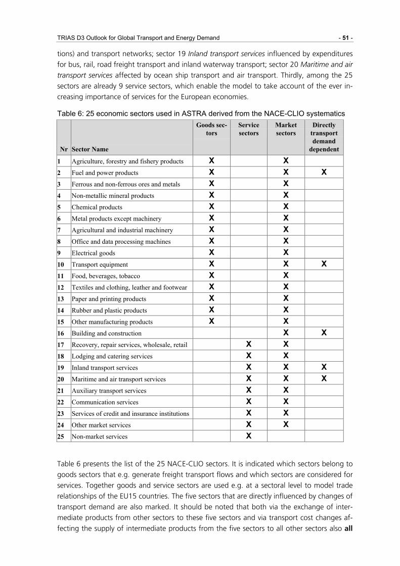
TRIAS D3 Outlook for Global Transport and Energy Demand - 51 -
tions) and transport networks; sector 19 Inland transport services influenced by expenditures
for bus, rail, road freight transport and inland waterway transport; sector 20 Maritime and air
transport services affected by ocean ship transport and air transport. Thirdly, among the 25
sectors are already 9 service sectors, which enable the model to take account of the ever in-
creasing importance of services for the European economies.
Table 6: 25 economic sectors used in ASTRA derived from the NACE-CLIO systematics
Nr Sector Name
Goods sec-tors
Service sectors
Market sectors
Directly transport demand
dependent
1 Agriculture, forestry and fishery products X X 2 Fuel and power products X X X 3 Ferrous and non-ferrous ores and metals X X 4 Non-metallic mineral products X X 5 Chemical products X X 6 Metal products except machinery X X 7 Agricultural and industrial machinery X X 8 Office and data processing machines X X 9 Electrical goods X X 10 Transport equipment X X X 11 Food, beverages, tobacco X X 12 Textiles and clothing, leather and footwear X X 13 Paper and printing products X X 14 Rubber and plastic products X X 15 Other manufacturing products X X 16 Building and construction X X 17 Recovery, repair services, wholesale, retail X X 18 Lodging and catering services X X 19 Inland transport services X X X 20 Maritime and air transport services X X X 21 Auxiliary transport services X X 22 Communication services X X 23 Services of credit and insurance institutions X X 24 Other market services X X 25 Non-market services X
Table 6 presents the list of the 25 NACE-CLIO sectors. It is indicated which sectors belong to
goods sectors that e.g. generate freight transport flows and which sectors are considered for
services. Together goods and service sectors are used e.g. at a sectoral level to model trade
relationships of the EU15 countries. The five sectors that are directly influenced by changes of
transport demand are also marked. It should be noted that both via the exchange of inter-
mediate products from other sectors to these five sectors and via transport cost changes af-
fecting the supply of intermediate products from the five sectors to all other sectors also all

- 52 - Economic, Transport and Environmental Modelling
sectors will be influenced by changes in the transport system that might emerge on a level as
detailed as a single OD-pair.
4.1.3 ASTRA Model Improvements
This section concentrates on the technical improvements developed and implemented in the
nine ASTRA modules. One task that is not reported specifically for each module concerns the
extension of the simulation horizon until 2050 from 2030. This required for exogenous vari-
ables to specify a development after 2030. The ASTRA merger and the related software re-
engineering, which constitute a tremendous improvement of ASTRA in terms of software
development, are described in the separate section 4.1.5.
4.1.3.1 Population Module
The previous ASTRA population module (POP) is characterised as a sophisticated one-year-
age cohort model. Hence there was no need to improve the structure of the POP module for
the TRIAS project. Nevertheless the POP module was recalibrated for the TRIAS project. In
order to synchronize the ASTRA demographic forecasts with recent EUROSTAT baseline pro-
jections (February 2006) until 2050 the calibration period has been prolonged from 1990 to
2050. Factors like country-specific death rates, migration balance and immigration age co-
horts were calibrated with the Vensim™ optimiser. Finally the calibration provided good qual-
ity results with less than 1% deviation to EUROSTAT baseline projections at maximum.
4.1.3.2 Macroeconomics Module
Improvements of the macroeconomic module (MAC) of ASTRA have not been a key task in
TRIAS. Hence, improvements were limited to three areas:
• Re-calibration of the endogenous GDP development such that development after
2050 becomes comparable with other forecasts, in particular of the European pro-
ject ADAM.
• Implementation of structure of fuel prices for alternative fuels that enables first to
distinguish the different elements of the fuel price (resource price, fuel tax, carbon
tax and VAT on fuel), and second to link with POLES and the BIOFUEL model that
calculate the fuel prices in TRIAS.
• Implementation of shifted and additional types of investments that result from the
different policies. This includes investments into biofuel production plants and hy-
drogen production plants that were provided by POLES and BIOFUEL, shift of in-
vestments due to the development and introduction of hydrogen fuel cell vehicles
into the car fleet and of R&D- and manufacturing plant investments due to en-
forced CO2 emission standards.
Implementation of fuel prices and fuel taxes

TRIAS D3 Outlook for Global Transport and Energy Demand - 53 -
Gasoline, diesel and kerosene fuel prices in ASTRA were already implemented with a struc-
ture distinguishing the pure fuel price, the fuel taxes and the VAT on fuel, while for other
fuels only simplified aggregate prices were used. Hence, in a first step the three-part struc-
ture was implemented for compressed natural gas (CNG), liquefied petroleum gas (LPG), hy-
drogen, bioethanol (first and second generation), biodiesel (first and second generation) and
electricity, and an exogenous trend for the ASTRA model was implemented. In a second step
for all fuels besides kerosene a link was implemented to the POLES and BIOFUEL model,
where POLES provides the inputs for gasoline, diesel, CNG, LPG, hydrogen and electricity and
BIOFUEL the inputs for biodiesel and bioethanol. A switch was implemented enabling to run
ASTRA stand-alone with its own implemented prices or linked to POLES and BIOFUEL.
All fuels were linked with a number of models of ASTRA where fuel prices or taxes play a
role. This includes the transport cost and modal choice (TRA), vehicle purchase decisions
(VFT), transport consumption expenditures (MAC) and tax revenues (MAC).
Considering investments into biofuel plants
The BIOFUEL model calculates the additional investments needed to build biofuel production
plants in order to satisfy the demand calculated by ASTRA and the BIOFUEL model itself.
These investments are transferred to ASTRA and become part of final demand. Since they are
provided as aggregate numbers they have to be split onto the ASTRA sectors to be consid-
ered properly in the investment model. The applied sectoral shares to split onto ASTRA sec-
tors are shown in Table 7.
Table 7: Split of aggregate biofuel plant investments onto ASTRA sectors
Sector Share [%] Sector Share [%] Minerals 35 Trade 7 Metal Products 7 Transport Inland 2 Industrial Machines 20 Other Market Services 5 Electronics 15 Non Market Services 1 Construction 8 Total 100
Source: EC Impact Assessment on Renewable Energies
Considering investments into hydrogen plants
Based on the fuel demand for hydrogen for Europe coming from ASTRA the POLES model
analyses which pathways for hydrogen production will be used. Two outcomes of this analy-
sis are transferred to ASTRA: hydrogen fuel cost (see above) and required investments into
hydrogen production plants and hydrogen infrastructure. The investments are provided as
aggregate numbers and hence have to be split onto the ASTRA sectors to become part of the
investment model of ASTRA. The applied sectoral shares to split onto ASTRA sectors are
shown in Table 8.

- 54 - Economic, Transport and Environmental Modelling
Table 8: Split of aggregate hydrogen plant investments onto ASTRA sectors
Sector Metal products Machinery Electronics Construction Share [%] 10 50 20 20
Source: ASTRA implementation for MATISSE project
Concerning hydrogen cars TRIAS follows the conclusion of the HyWays project that the first
hydrogen cars have to be subsidised to bring them into the market. Hence, in the first ten
years when hydrogen cars enter the market the related subsidies are calculated and the sub-
sidies become part of government expenditures and of national income.
Considering the shift of consumption and investments due to fuel cells in cars
Cars equipped with hydrogen fuel cells have to be manufactured differently then cars with
internal combustion engines. The former require less moving parts and a higher contribution
of electronics and chemicals sectors for the production of the fuel cells and their drive train.
This means the demand for hydrogen fuel cell cars from private consumers and businesses
affects other sectors then if these customers would buy cars with combustion engines. In the
ASTRA model this is taken into account by extracting the share of car purchase cost that is
related to the engine (34%) and distributing part of this demand onto the electronics sector
(40% of drive train cost) and chemicals sector (30% of drive train cost). The remaining 30%
of the drive train cost are still supplied by the vehicles sector. This split of demand is imple-
mented for both the demand of private consumers that becomes part of sectoral consump-
tion in ASTRA and the demand of businesses for cars that becomes part of sectoral invest-
ments.
Considering investments to reduce CO2 emissions of cars
ASTRA has incorporated CO2 emission factors for EURO 1 to EURO 7 type of cars. After 2025
a further exogenous reduction trend of CO2 emission factors is assumed for baseline scenario
(-35% from 2025 until 2050, see also section 4.1.4.7). This trend is also reflected in the car
prices. Policies that require more ambitious reduction efforts lead to lower emission factors,
to additional investments into R&D and fuel consumption and emissions and upgraded
manufacturing plants and hence to higher car prices. This is reflected in ASTRA by calculating
the additional turnover from car purchase compared to the baseline and by assigning these
revenues to additional investments onto the two sectors other-market-services (60% of addi-
tional investments) and machinery (30%). This approach ensures both that the technical im-
provements do not fall from haven like manna, that additional investments appear in the
economic framework and that the budget constraint is considered, which is implemented as
part of the ASTRA consumption model i.e. when consumers spend more money for transport
purposes they have less to spent for other sectors of the economy.
4.1.3.3 Foreign Trade Module
The foreign trade module (FOT) was extended to consider the change of imports of fossil
fuels that would occur due to the policies. Two versions are implemented that affect the im-

TRIAS D3 Outlook for Global Transport and Energy Demand - 55 -
ports of the energy sector of the EU29 countries from the rest-of-the-world in monetary
terms:
• ASTRA includes an endogenous import model for the energy sector, which is cali-
brated to OECD and EUROSTAT statistics. Based on the expenditures for gasoline,
diesel, CNG and LPG without any taxes the changes of expenditures for fossil fuels
are calculated for each EU29 country. Assuming that none of these countries is able
or willing to change significantly its domestic production or its imports from other EU
countries, such changes of fossil fuel consumption would affect the imports from the
rest-of-the-world. For instance, when less fossil fuel is used for transport due to shift
to alternative fuels that would reduce the imports of the energy sector and hence
would generate a positive stimulus on the demand side of the economy.
• In the linkage with POLES the approach is implemented differently. POLES includes a
world energy trade model and receives from ASTRA the changed transport fuel de-
mand including the fossil fuel types. Based on this information POLES provides the
fossil fuel imports to ASTRA, which are then feeding into the imports of the energy
sector.
4.1.3.4 Transport Module
The transport module has been subjected to many modelling tasks in order to contribute to
the development and improvement of the ASTRA model. In particular, the following activities
have been completed:
Transport passenger:
revision of modal split algorithm in order to take into account car ownership;
update of passenger data stocks;
implementation of new transport costs;
re-calibration of the module according to last data and trend available.
Transport freight:
introduction of road feeder mode for rail and ship;
including selected OD pair from EU12 to EU15 countries (and vice-versa) in the MED
distance band;
update of freight data stocks;
implementation of new transport costs;
re-calibration of the module according to last data and trend available.

- 56 - Economic, Transport and Environmental Modelling
Transport Passenger Sub-Module (TRA pass)
Revision of modal split algorithm to take into account car ownership
This task consisted in testing and calibrating the addition of a specific car-ownership parame-
ter in the modal split function. The expected role of this parameter is to increase the share of
car when motorisation rate increases (other things – times, costs, modal constants – being
equal).
The car-ownership effect on modal split has been tested introducing in the generalised cost
used for modal split an additional term depending on car ownership yearly growth rate de-
velopment during the time simulation period. The additional term, representing this effect,
multiply the “original” generalised cost, so its value is between 0 and 1: as the independent
variable of this function is the index of the car ownership yearly growth rate, the additional
term has been included as a lookup depending on this variable, in order to reflect the
changes occurred every year. Different lookups for local and medium-long distances have
been used, with a lower effect for the latter, as well as for EU15 and EU12 countries. The
effect of the new term is to slightly reduce the generalized cost of car on all O/D pairs as the
car-ownership of the origin country increases (on the contrary, in case the car ownership rate
is negative the value of the variable is higher than 1, so the original generalized cost is slightly
increased). At local level, the lookup is also differentiated by functional zone of origin (the
effect is stronger in sparsely regions and lower in metropolitan area).
Index Car Ownership Yearly growthrate
gen costper trip car ownership effectMD modalsplit
gen costper trip corr
PassVol Calc Vaclav
gen cost per trip car ownership effect onMD modalsplit
gen cost per trip corr
PassVol Calc Vaclav
Index Car Ownership Yearly growthrate
gen costper trip car ownership effectMD modalsplit
gen costper trip corr
PassVol Calc Vaclav
gen cost per trip car ownership effect onMD modalsplit
gen cost per trip corr
PassVol Calc Vaclav Figure 27: Structure of the car-ownership effect on modal split
Passenger Data Stocks Update
The data for the stocks which are used as starting point for the ASTRA model runs has been
completely re-estimated using more updated information (where available). Data concerning
passenger in terms passenger and passenger*km has been selected from the SCENES data
(version 2005, for the White Paper Assessment project). The SCENES model produces data
for passenger concerning:
passengers traffic (Million pass/year) by O/D pair, purpose and mode;
passengers average distance (km) by O/D pair, purpose and mode;

TRIAS D3 Outlook for Global Transport and Energy Demand - 57 -
The terms O/D pair, purpose, flow and mode, used above are to be intended with the mean-
ing used in ASTRA. The correspondence between the ASTRA concept and the SCENES ele-
ments is described in the following paragraph.
Three trip purposes are considered in ASTRA for the passenger demand, which correspond to
the SCENES flows as explained in the following table.
Table 9: Conversion between SCENES flows and ASTRA purposes ASTRA Purpose SCENES flow Business 20-21-26-27-28
Personal 18-19-29-30-31-32
Tourism 22-23-24-25
The modes used in ASTRA for passengers in terms of the SCENES ones is explained in the
following table.
Table 10: Conversion between SCENES modes and ASTRA modes ASTRA passenger mode SCENES mode
Slow 11
Car 1 – 12
Bus/coach 2
Train 3 – 4 – 13
Air 5 – 16 – 17
The main issue in the extraction of SCENES data is the classification of O/D pairs. Modes,
flows and purposes can be readily obtained according by aggregation of the SCENES vari-
ables, O/D pairs are more difficult to deal with.
The problem is that traffic from a given origin (defined as country + functional zone) and a
given destination (defined as country + functional zone) is to be further divided into the dif-
ferent distance bands to yield the complete O/D definition. If the output of the SCENES
model is aggregated just on the basis of the functional classification of each zone (e.g. by
defining High Density Areas of Italy, of France, etc.) the total amount of demand for each
O/D is derived, without any reference to the distance other than the average distance.
In order to extract the data and recognise the different groups of demand, the SCENES O/D
pairs have been extracted and classified according to the ASTRA criteria “country origin,
functional zone origin, country destination, functional zone destination, distance band”,
where the distance band has been assigned on the basis of the average distance calculated.
Once that the data has been converted into a format consistent with ASTRA definition, the
resulting matrix has been used to calculate the passenger traffic by OD pair, flow and mode
(in terms of pass/year and pass*km/year) and to compare the aggregated results with Euro-
stat total pkm per country in 2000 (Transport in figures 2005).
As some discrepancies have been detected, some adjustments have been produced in order
to reflect Eurostat aggregated data. The new corrected matrix has been used to recalculate

- 58 - Economic, Transport and Environmental Modelling
the passenger traffic by OD pair, flow and mode, with the results that the aggregated com-
parison with Eurostat total pkm per country in 2000 was acceptable.
Table 11: Comparison between data stock and Eurostat total pkm per country in 1990 and 2000
Observed pkm (Eurostat, elab TRT)
Data stocks (SCENES, elab. TRT)
Difference (%) Country
1990 2000 1990 2000 1990 2000
Austria 84 677 108 555 83 786 107 044 -1% -1%
Belgi-um&Luxembourg 115 896 141 733 112 314 137 317 -3% -3%
Denmark 65 792 80 395 62 038 75 698 -6% -6%
Spain 258 377 438 394 264 932 448 307 3% 2%
Finland 67 354 73 387 58 637 63 828 -13% -13%
France 719 022 850 760 713 820 843 480 -1% -1%
Great Britain 705 657 787 096 661 966 739 839 -6% -6%
Germany 847 602 1 027 721 811 457 981 305 -4% -5%
Greece 81 542 123 759 80 848 123 066 -1% -1%
Ireland 25 217 33 806 26 164 34 811 4% 3%
Italy 670 469 900 773 666 226 891 434 -1% -1%
The Netherlands 167 007 175 109 182 664 190 852 9% 9%
Portugal 62 409 111 445 59 957 104 934 -4% -6%
Sweden 111 944 124 649 103 293 114 399 -8% -8%
Bulgaria 39 293 26 162 37 045 24 918 -6% -5%
Switzerland 102 354 124 792 92 155 113 669 -10% -9%
Cyprus 8 131 10 152 6 663 8 438 -18% -17%
Czech Republic 76 256 90 581 68 582 81 867 -10% -10%
Estonia 11 368 12 148 9 907 10 497 -13% -14%
Hungary 78 639 76 645 69 875 68 139 -11% -11%
Latvia 13 699 12 407 11 773 10 590 -14% -15%
Lithuania 18 614 19 066 16 004 17 187 -14% -10%
Malta 3 141 3 894 2 754 3 503 -12% -10%
Norway 59 382 73 724 58 589 73 634 -1% 0%
Poland 172 733 202 856 152 769 181 021 -12% -11%
Romania 59 234 28 831 60 847 28 453 3% -1%
Slovenia 15 830 17 693 15 459 18 767 -2% 6%
Slovakia 32 857 35 619 31 407 33 784 -4% -5%
Total 4 674 496 5 712 152 4 521 935 5 530 781 -3% -3%

TRIAS D3 Outlook for Global Transport and Energy Demand - 59 -
Implementation of New Transport Modes Costs
For most of the modes of transport, a new, more detailed, structure of costs has been im-
plemented. Values to fill in the new variables have been estimated from different sources.
The revision of transport cost has mainly involved all the passenger modes: car, train, bus
(local and long distance) and – in a different way – air transport. For all modes (except air
passenger) the structure of the calculation is similar and is designed to produce as main out-
put the average cost per Pass*km of every mode. This result is used in the mode split algo-
rithm and other intermediate outputs like taxation unitary revenues.
The new structure implemented is exactly the same for all EU25 countries. This means that
also where in the original version of the model a different structure was used for EU15 and
NMS, now the cost is computed in the same way and with the same level of detail.
In general, the new cost structure and the new data implemented came up with final costs
that in many cases are quite different from the original ones. Therefore, a recalibration of the
mode split modules has been required.
Private Car Costs
The costs are divided into five main categories, according to common specifications found in
literature. Taxes, that influence investment and fuel, are kept separated to be used in other
parts of the model. Therefore, for instance, fuel cost per vkm is actually the result of three
components: pure fuel price, excises and VAT on fuel (the same structure already existing in
ASTRA).
The calculation structure (see Figure 28) produces two kinds of costs: the perceived one (to
be used in the modal choice) and the total one (representing consumed resources plus taxes).
investment per vkm
maintenance per vkm
fuel per vkm
toll per vkm
car PRODUCTION cost per vkm, engine, distance
Costs included Total cost Total cost aggregated
car PRODUCTION cost pervkm
car PERCEIVED cost per vkm
car PERCEIVED cost per vkm, engine, distance
Figure 28: Car cost split
The costs are fully split, depending on fuel and emission class and then weighted with fleet
for obtaining the final indicator. Actually, tolls are not computed within the cost per vkm, but
are included later in the transport module at the O/D pair level.
For the cost estimation data is fully available for Italy (Italian Automobile Club publishes an
annual collection of fully split costs: ACI, 2006). Some information is available for UK, too
(AA Trust, 2006). For all other countries the Maintenance costs, Investment costs, Insurance
costs derive from Italian ones with the application of the same proportion found for trucks.
For instance, the hypothesis is that the proportion between Italian and German cost of tires is
the same for trucks and cars.

- 60 - Economic, Transport and Environmental Modelling
Taxation levels, both for purchase and periodic taxes, are available for some countries (Den-
mark, Netherlands, Ireland, Greece, Finland, Italy, Austria, Germany, Great Britain). The
sources of such data are TIS, 2002 and OECD/EEA, 2006.
The costs data used are reported in the following table.
Table 12: Data found for car costs. Country Purchase PurchaseTaxes Yearly taxes Insurance Maintenance
[€/vehicle] [€/vehicle] [€/year] [€/year] [€/km]
ITA 16 845 171 170 1 349 0.075
AUT 17 695 1 388 212 650 0.065
FRA 16 334 1 080 0.068
GER 16 334 100 360 1 160 0.062
POL 13 952 474 0.043
SLO 15 313 846 0.052
ESP 16 504 707 0.052
HUN 16 504 402 0.046
GBR 17 525 171 278 638 0.049
DNK 15 659 463
NLD 4 625 307
IRL 4 423 306
GRC 2 667 133
FIN 7 503 186 * including VAT Sources: ACI (2006), AA Trust (2006), OECD/EEA (2006), TIS (2002)
In order to use available data to estimate costs for all countries, equivalence tables have been
defined. Table 13 reports the two tables, one used for taxation and the other for remaining
cost components.
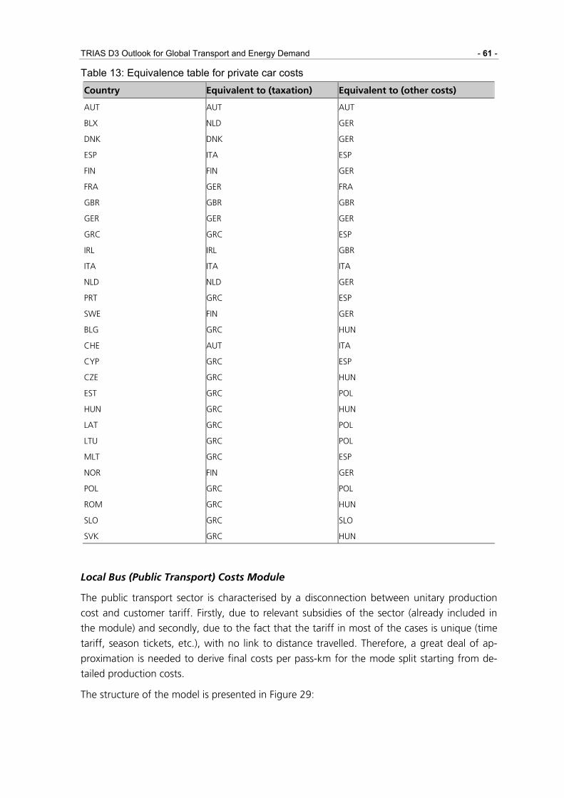
TRIAS D3 Outlook for Global Transport and Energy Demand - 61 -
Table 13: Equivalence table for private car costs
Country Equivalent to (taxation) Equivalent to (other costs)
AUT AUT AUT
BLX NLD GER
DNK DNK GER
ESP ITA ESP
FIN FIN GER
FRA GER FRA
GBR GBR GBR
GER GER GER
GRC GRC ESP
IRL IRL GBR
ITA ITA ITA
NLD NLD GER
PRT GRC ESP
SWE FIN GER
BLG GRC HUN
CHE AUT ITA
CYP GRC ESP
CZE GRC HUN
EST GRC POL
HUN GRC HUN
LAT GRC POL
LTU GRC POL
MLT GRC ESP
NOR FIN GER
POL GRC POL
ROM GRC HUN
SLO GRC SLO
SVK GRC HUN
Local Bus (Public Transport) Costs Module
The public transport sector is characterised by a disconnection between unitary production
cost and customer tariff. Firstly, due to relevant subsidies of the sector (already included in
the module) and secondly, due to the fact that the tariff in most of the cases is unique (time
tariff, season tickets, etc.), with no link to distance travelled. Therefore, a great deal of ap-
proximation is needed to derive final costs per pass-km for the mode split starting from de-
tailed production costs.
The structure of the model is presented in Figure 29:

- 62 - Economic, Transport and Environmental Modelling
fuel per vkm
labour per vkm
subsidies per vkm
Bus TOTAL cost per vkm, engine Bus TOTAL cost per vkm
Bus NET cost per vkmBus NET cost per vkm,
engine
calc TARIFF, per country
investment per vkm
maintenance per vkm
pkm TARIFF, per country
Figure 29: Urban bus cost split
As tariffs cannot be calculated precisely due to the weak link between costs and tariff, values
to be used in the logit model, is calculated as follows:
cc
cC TCC
LFANCT *= (eq. 1)
where: Tc = tariff for country c ANCc = Average Net Cost per vkm for country c LFc = Load factor for country c TCCc = Calibration cost coefficient for country c
The coefficient TCCc has been calibrated during the overall calibration process of the TRA
module.
The module calculates an alternative definition of the tariff using the average number of pas-
senger trip on local bus. This computation is done essentially to check that the size of costs is
reasonable.
For the cost estimation data about total costs and subsidies, expressed in €/vkm, is available
for some Italian cities (elaboration of Cambini et Galleano, 2005 and Dell’Aringa, 2004) and
for a selection of Western European countries (Earchimede, 2005).
Although elaborating the two Italian sources one can found a complete set of data, we chose
to use the source Earchimede (2005) due to the fact that it was the only one including com-
parative information about some European countries. Nothing is available for Eastern Europe.
Cross-checking the two sources it has been found that data concerning franchising competi-
tions (Cambini et Galleano, 2005 and Dell’Aringa, 2004) are considerably higher than the
used source (Earchimede, 2005): for Italy a cost of 3.5€/vkm instead of a calculated average
of 5€/km. Nevertheless the source is trustworthy and is the only one we have been able to
find with international data split according to homogeneous categories of costs and the
comparable across countries. The same source suggests values for subsidies, too.
The data collected are in Table 14. The cost of fuel used is endogenously calculated. The
numbers reported in table have been used for verification.

TRIAS D3 Outlook for Global Transport and Energy Demand - 63 -
Table 14: Available data on bus costs. Country Labour Cost Purchase Maintenance Fuel Subsidies
[€/vkm] [€/vkm] [€/vkm] [€/vkm] [€/vkm]
ITA 2.30 0.30 0.58 0.316 2.20
GBR 0.80 0.17 0.50 0.333 0.60
GER 2.10 0.35 1.28 0.269 1.50
FRA 1.60 0.36 0.69 0.249 1.90
SWE 1.10 0.20 0.31 0.286 0.90
NLD 1.70 0.30* 0.10 0.297 1.50
BLX 2.00 0.29 0.41 0.299 2.00 * Estimated value Sources: Earchimede (2005)
The data collected has been expanded to the whole Europe, according to the equivalence
reported in Table 15.
Table 15: Equivalence table for bus costs. Country code Equivalent to Country code Equivalent to
AUT GER BLG ITA
BLX BLX CHE FRA
DNK SWE CYP ITA
ESP ITA CZE ITA
FIN SWE EST ITA
FRA FRA HUN ITA
GBR GBR LAT ITA
GER GER LTU ITA
GRC ITA MLT ITA
IRL GBR NOR GER
ITA ITA POL ITA
NLD NLD ROM ITA
PRT ITA SLO ITA
SWE SWE SVK ITA
Long Distance Bus Costs Module
Long distance buses are defined here as private coach services operating on inter-regional,
national and international routes as well as tourist buses. Their cost structure is similar to that
used for the public transport services, with the difference that year tolls are considered. Cur-
rently, long distance buses are probably not subsidised, but subsidies are included in the
structure anyway for policy purposes (e.g. shifting subsidies from rail to coaches).
The structure of the module is the following:

- 64 - Economic, Transport and Environmental Modelling
labour per vkm
investment per vkm
maintenance per vkm
fuel per vkm
toll per vkm
bus production cost per vkm, engine, distance
bus production cost per vkm, distance
subsidies per vkm
Costs included Total cost Total cost aggregated
Bus TARIFF
Figure 30: Non-local bus cost split
Unfortunately we have not been able to find any data about coach companies costs in
Europe. For estimation some data coming from a periodic publication (Autobus, 2005) de-
scribing unitary exercise costs has been used. Since the contents just refers to Italy and does
not include all elements required to define each cost components, some hypotheses have
been done, in particular:
The labour costs for long distance buses have been calculated applying to the urban
bus value the ratio obtained from Autobus (2005). For Italy this ratio is 65%, while
for other countries has been supposed lower.
The investment and maintenance unitary costs are approximately half for intercity
buses compared to urban buses. The same ratio has been applied to all countries.
The fuel cost ratio is about 80%, applied to all countries.
Subsidies are supposed to be zero.
Costs have been first estimated using the assumptions above for the countries for which ur-
ban bus costs were available (see section 3); Table 16 reports such a data. Therefore data
have been extended to the other countries using the same equivalence table used for urban
buses (see Table 15). The cost of fuel used is endogenously calculated. The numbers reported
in table can be used for verification.
Table 16: Data estimated for long distance bus costs. Country Labour Cost Purchase Maintenance Fuel Subsidies
[€/km] [€/km] [€/km] [€/km] [€/km]
ITA 1.50 0.15 0.29 0.253 0
GBR 0.80 0.09 0.25 0.267 0
GER 1.68 0.18 0.64 0.215 0
FRA 1.28 0.18 0.35 0.199 0
SWE 0.88 0.10 0.16 0.229 0
NLD 1.36 0.15 0.05 0.237 0
BLX 1.60 0.15 0.21 0.240 0 Sources: own estimations on Autobus (2005) and Earchimede (2005) data.

TRIAS D3 Outlook for Global Transport and Energy Demand - 65 -
Train Costs Module
The structure of the costs is the same for both passenger and freight trains, also because
railway companies usually are not able to distinguish labour costs of energy costs, etc, by
type of service. Anyway, two different views have been dedicated to the transport by train
for passenger and freight. Like for local bus, subsidies are very important in the cost struc-
ture, and like for bus it is however difficult to link total productions costs, subsidies and tar-
iffs.
The following figure represents the structure of the module for passenger services.
Costs included Total cost Total cost aggregated
TrainPax TOTAL cost per vkm
TrainPax NET cost per vkm
TrainPax TARIFF, pervkm, per country
fuel/energy per vkm
labour per vkm
subsidies per vkm, per service
TrainPax TOTAL cost per vkm
TrainPax NET cost per vkm
investment per vkm
maintenance per vkm
infrastr. access per vkm
TrainPax COST, perseatkm, per country
Figure 31: Train passenger cost split
For cost estimation for Italy is available an official document (Cicini et al, 2005) detailing costs
splitting for single voices and for different services (local, intercity, high speed, freight).
A complete survey of average costs of rail companies in Europe can be derived from UIC data
(even if the last available data refers to 1999). Using the total expenditures and revenues for
exercise and the total amount of train*km produced, average cost values for an average train
type. Split of costs for different services (local, long, high speed, freight) has been estimated
using the proportions of different costs for Italian railways.
The cost for energy provided is the one of large industrial clients in Italy. In any case the
amount of energy costs per train*km is extremely limited in comparison to other components
(about 4%).
The cost for access to infrastructure could be determined using the official documents for
Italy only. For other countries UIC data for infrastructure access costs are quite incomplete
(also because data concerns year 1999 and in many countries such a cost has not been exist-
ing until very recent time), so this item has been disregarded.
Table 17 reports Italian data while Table 18 provides average data for all countries estimated
using UIC data and equivalences reported in Table 19.

- 66 - Economic, Transport and Environmental Modelling
Table 17: Data for Italian train costs derived from Cicini et al, (2005)
Service type Labour Investment Maintenance Energy
Infrastructure access
Other
[€/km] [€/km] [€/km] [€/kWh] [€/km] [€/km]
Intercity 3.74 4.48 2.05 0.084 2.11 1.28
Local 3.80 3.44 1.60 0.084 2.727 1.28
Freight 5.00 2.40 1.90 0.084 2.727 0.57 Sources: Cicini et al (2005).
Table 18: Data for train costs, taken from UIC (1999)
Country Labour Investment Maintenance
Infrastruc-ture access
Subsidies Other
[€/km] [€/km] [€/km] [€/km] [€/km] [€/km]
AUT 13.54 2.42 5.26 1.82 4.282 1.34
BLX 17.65 4.29 8.14 - 4.639 1.31
DNK 6.59 - 5.72 0.33 - 0.93
ESP 6.14 2.85 4.92 - 1.690 2.37
FIN 7.81 1.89 4.21 1.20 0.787 0.39
FRA 13.47 1.82 8.73 2.92 5.571 5.36
GER 9.85 2.09 10.42 0.00 1.708 0.77
GRC 14.63 2.58 3.42 - 0.049 7.20
IRL 10.74 2.00 10.40 - 3.452 0.96
ITA 13.91 5.64 6.47 - 9.963 0.41
NLD 7.73 2.02 13.47 - 6.001 1.11
PRT 6.82 1.91 6.03 - 0.691 2.25
SWE 4.52 0.93 6.16 0.26 - 0.83
CHE 14.60 5.54 6.60 - 8.951 0.87
CZE 3.97 1.09 2.85 - 1.547 0.33
HUN 3.18 0.65 2.73 - 4.067 0.33
NOR - 1.24 7.81 - 3.362 0.53
POL 4.64 1.65 2.35 - 1.296 0.99
ROM 2.58 0.19 7.22 - 2.183 0.30
SLO 5.65 1.48 5.00 - 2.395 1.03
SVK 4.10 1.10 3.50 - 2.851 2.13 Sources: own elaboration on Cicini et al (2005) and UIC (1999) data

TRIAS D3 Outlook for Global Transport and Energy Demand - 67 -
Table 19: Equivalence table for train costs
Country code Equivalent to Country code Equivalent to
AUT AUT BLG ROM
BLX BLX CHE CHE
DNK DNK CYP n.r.
ESP ESP CZE CZE
FIN FIN EST POL
FRA FRA HUN HUN
GBR IRL LAT POL
GER GER LTU POL
GRC GRC MLT n.r.
IRL IRL NOR NOR
ITA ITA POL POL
NLD NLD ROM ROM
PRT PRT SLO SLO
SWE SWE SVK SVK
Air Passenger Cost
The structure for the calculation of air passenger costs has been slightly changed. Currently,
the model already distinguishes fuel and non-fuel costs. Adding further details needed to
introduce the distinction between conventional airlines and budget (low cost) companies,
which has been done in a simplified way.
The non-fuel cost is calculated as weighted average between the conventional airlines cost
(the old cost in the model) and the budget companies cost (estimated on the basis of several
OD pair and companies around 0.07 euro/km). The share of the low cost companies has
been calibrated in order to reflect the growth that they had during the last years.
Effects of Passenger Cost Update on Policy Simulation
With the proposed structure for passenger cost there are some policies that can be simulated
in more detail than in the current version of the model. For instance:
differential taxation for innovative vehicles (both purchase and fuel taxes);
change of labour costs due to social legislation, market structure, etc.
car pooling.
Subsidies system: the amount of subsidies transferred to public transport can vary to
assess the effects both to modal split module and macroeconomic effects module;
Fleet renewal (in terms of expenditures and therefore impacts on the economic side);
Public transport companies downsizing due to liberalisation.
Modifications in the subsidies structure between modes (from train to bus);
Effect of older vehicles substitution.
- 68 - Economic, Transport and Environmental Modelling
Effects due to liberalisation (fleet renewal, price lowering, cost lowering).
Transport Freight Sub-Module (TRA Fre)
Modelling Road Feeder Traffic for Rail and Ship
In many instances, a door-to-door consignment by rail and sea shipping requires that trucks
are used for feeding the main mode (a train or a vessel). Given the aggregate description of
modes in ASTRA, this circumstance cannot be simulated in detail. However, in order to avoid
the underestimation of road tkm and overestimation of the other modes, a correction has
been implemented to the amount of tkm of rail and ship. The size of the correction has been
calculated on the basis of tkm data of a sample of OD pairs from SCENES. The calculated
share of traffic to be assigned to truck is different for ship and rail - about 14% for rail and
9% for ship. The correction has been applied to total tkm of rail and ship modes and added
to road mode after the modal split.
Including selected OD pair from NMS to EU15 countries and vice-versa in the MED freight distance band
In the previous version of the ASTRA, the EU15 and the more recent EU partners were con-
nected only in the long distance band (>700 km). In order to improve the description of the
demand between these two groups of countries, a number of O/D pairs have been included
also in the medium MED distance band (150-700 km). The relevant O/D pairs have been se-
lected from the analysis of the ETIS BASE and SCENES data.
Implementation of Revised Transport Costs
The revision of transport cost has mainly involved the following freight modes: truck, train
and partially ship. For all modules (except ship) the structure of the calculation is similar and is
designed to produce as main output the average cost per vehicle*km of every mode. This
result is used in the mode split algorithm and other intermediate outputs like taxation unitary
revenues.
The new structure implemented is exactly the same for all EU25 countries. This means that
also where in the original version of the model a different structure was used for EU15 and
NMS, now the cost is computed in the same way and with the same level of detail. Even if
checks have been performed that this change did not give rise to problems in other parts of
the model, this aspect should be taken into account.
All modules are designed to produce one main output, the average cost per vehicle*km of
every mode to be used in the mode split algorithm, and other intermediate outputs like taxa-
tion unitary revenues.
In general, the new cost structure and the new data implemented came up with final costs
that in many cases are quite different from the original ones. Therefore, a recalibration of the
mode split modules has been required.

TRIAS D3 Outlook for Global Transport and Energy Demand - 69 -
Truck Costs Module
The module is structured as follows (Figure 32).
labour per vkm
investment per vkm
maintenance per vkm
fuel per vkm
toll per vkm
truck production cost per vkm, engine, distance
truck production cost per vkm, per engine, distance,
OD functional zones
LOC:MED:LGD:
REG:
Costs included Total cost Total cost aggregated
truck production cost per vkm, cargo type, distance
truck production cost pervkm, cargo type, distance,
OD functional zones
Figure 32: Road freight cost split
The costs are divided into five main categories, according to common specifications found in
literature. Taxes, that influence investment and fuel, are kept separated to be used in other
parts of the model. Therefore, for instance, fuel cost per vkm is actually the result of three
components: pure fuel price, excises and VAT on fuel (the same structure already existing in
ASTRA).
In the model, the tolls for REG transport are, differently from other distance classes, specified
for different functional zones. That’s why the final output is different between regional and
other three distance classes. Also, tolls are not actually computed within the cost per vkm,
but are included later at the O/D pair level.
The module reflects the cost structure of a document produced for Italian Ministry and the
syndicate of truck operators5, which contains comparative numerical materials about costs of
truck transport. A cross-check has shown that total costs reported in this document are ex-
tremely similar to costs estimated for the TREMOVE II project (see note TRT-4 of TREMOVE II
project). Also fuel data seems consistent to the current values in ASTRA6. Therefore the
source looks reliable and reports a detailed desegregation of total cost. The data refers to
nine countries only (Italy, Austria, France, Germany, Poland, Slovenia, Spain, Hungary,
Ukraine), but with some assumptions (and with previous editions of the same document con-
taining different countries) it has been possible to extend the analysis to almost all EU coun-
tries.
The data elaborated for the nine countries are reported in Table 20 below. Costs per vehicle-
km have been obtained assuming an average yearly mileage of 100,000 km.
5 Centro Studi sui Sistemi di Trasporto, (2005), Indagine conoscitiva sui costi e sulla fiscalità sop-
portati dalle imprese italiane di autotrasporto…, Ministero dei Trasporti e della Navigazione, Roma (Italy).
6 In particular, the category for which ASTRA and the document produce the same result is the MED distance for HDV. Differences between emission classes are negligible.

- 70 - Economic, Transport and Environmental Modelling
Table 20: Original data on truck costs
Country Labor Cost Purchase
Purchase Taxes
Yearly taxes Insurance Maintenance
[€/year] [€] [€] [€/year] [€/year] [€/km]
ITA 45 923 153 439 1 399 718 8 067 0.194
AUT 47 083 123 550 160 4 029 3 888 0.157
FRA 53 044 131 929 278 730 6 455 0.154
GER 45 126 120 862 95 2 586 6 933 0.162
POL 21 580 127 992 120 890 2 833 0.104
SLO 32 453 136 167 - 3 600 5 059 0.124
ESP 33 005 130 221 66 788 4 230 0.129
HUN 22 858 135 226 160 1 097 2 406 0.111
UKR 18 765 111 245 105 775 2 373 0.089 Source: CSST, 2005
The following Table 21 summarises the equivalences used between countries. These equiva-
lences have been assumed from similarity of economic and welfare conditions, similarities in
markets, geographical proximity, etc.
Table 21: Equivalence table for truck costs Original Country Equivalent to Original Country Equivalent to
AUT AUT BLG HUN
BLX GER CHE ITA
DNK GER CYP ESP
ESP ESP CZE HUN
FIN GER EST POL
FRA FRA HUN HUN
GBR FRA LAT POL
GER GER LTU POL
GRC ESP MLT ESP
IRL FRA NOR GER
ITA ITA POL POL
NLD GER ROM HUN
PRT ESP SLO SLO
SWE GER SVK HUN
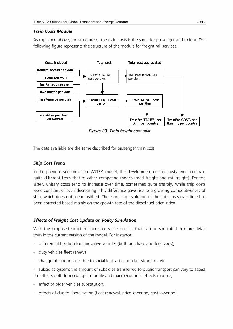
TRIAS D3 Outlook for Global Transport and Energy Demand - 71 -
Train Costs Module
As explained above, the structure of the train costs is the same for passenger and freight. The
following figure represents the structure of the module for freight rail services.
Costs included Total cost Total cost aggregated
TrainPax TOTAL cost per vkm
TrainFRE NET cost per tkm
TrainFre TARIFF, pertkm, per country
fuel/energy per vkm
labour per vkm
subsidies per vkm, per service
TrainPax TOTAL cost per vkm
TrainFRENET cost per tkm
investment per vkm
maintenance per vkm
infrastr. access per vkm
TrainFre COST, pertkm , per country
TrainFRE TOTAL cost per vkm
TrainFRE TOTAL cost per vkm
Costs included Total cost Total cost aggregated
TrainPax TOTAL cost per vkm
TrainFRE NET cost per tkm
TrainFre TARIFF, pertkm, per country
fuel/energy per vkm
labour per vkm
subsidies per vkm, per service
TrainPax TOTAL cost per vkm
TrainFRENET cost per tkm
investment per vkm
maintenance per vkm
infrastr. access per vkm
TrainFre COST, pertkm , per country
TrainFRE TOTAL cost per vkm
TrainFRE TOTAL cost per vkm
Figure 33: Train freight cost split
The data available are the same described for passenger train cost.
Ship Cost Trend
In the previous version of the ASTRA model, the development of ship costs over time was
quite different from that of other competing modes (road freight and rail freight). For the
latter, unitary costs tend to increase over time, sometimes quite sharply, while ship costs
were constant or even decreasing. This difference gave rise to a growing competitiveness of
ship, which does not seem justified. Therefore, the evolution of the ship costs over time has
been corrected based mainly on the growth rate of the diesel fuel price index.
Effects of Freight Cost Update on Policy Simulation
With the proposed structure there are some policies that can be simulated in more detail
than in the current version of the model. For instance:
- differential taxation for innovative vehicles (both purchase and fuel taxes);
- duty vehicles fleet renewal
- change of labour costs due to social legislation, market structure, etc.
- subsidies system: the amount of subsidies transferred to public transport can vary to assess
the effects both to modal split module and macroeconomic effects module;
- effect of older vehicles substitution.
- effects of due to liberalisation (fleet renewal, price lowering, cost lowering).
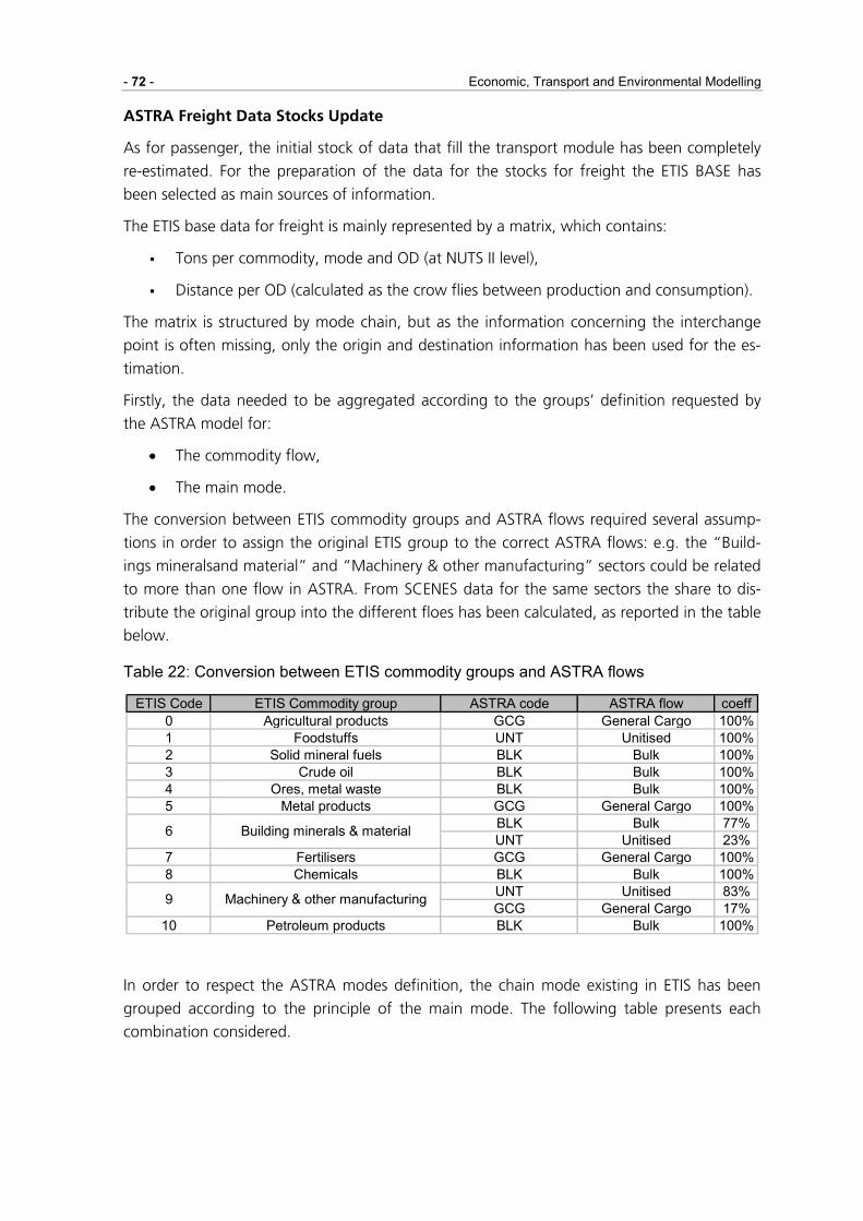
- 72 - Economic, Transport and Environmental Modelling
ASTRA Freight Data Stocks Update
As for passenger, the initial stock of data that fill the transport module has been completely
re-estimated. For the preparation of the data for the stocks for freight the ETIS BASE has
been selected as main sources of information.
The ETIS base data for freight is mainly represented by a matrix, which contains:
Tons per commodity, mode and OD (at NUTS II level),
Distance per OD (calculated as the crow flies between production and consumption).
The matrix is structured by mode chain, but as the information concerning the interchange
point is often missing, only the origin and destination information has been used for the es-
timation.
Firstly, the data needed to be aggregated according to the groups’ definition requested by
the ASTRA model for:
• The commodity flow,
• The main mode.
The conversion between ETIS commodity groups and ASTRA flows required several assump-
tions in order to assign the original ETIS group to the correct ASTRA flows: e.g. the “Build-
ings mineralsand material” and “Machinery & other manufacturing” sectors could be related
to more than one flow in ASTRA. From SCENES data for the same sectors the share to dis-
tribute the original group into the different floes has been calculated, as reported in the table
below.
Table 22: Conversion between ETIS commodity groups and ASTRA flows
ETIS Code ETIS Commodity group ASTRA code ASTRA flow coeff0 Agricultural products GCG General Cargo 100%1 Foodstuffs UNT Unitised 100%2 Solid mineral fuels BLK Bulk 100%3 Crude oil BLK Bulk 100%4 Ores, metal waste BLK Bulk 100%5 Metal products GCG General Cargo 100%
BLK Bulk 77%UNT Unitised 23%
7 Fertilisers GCG General Cargo 100%8 Chemicals BLK Bulk 100%
UNT Unitised 83%GCG General Cargo 17%
10 Petroleum products BLK Bulk 100%
Building minerals & material6
9 Machinery & other manufacturing
In order to respect the ASTRA modes definition, the chain mode existing in ETIS has been
grouped according to the principle of the main mode. The following table presents each
combination considered.

TRIAS D3 Outlook for Global Transport and Energy Demand - 73 -
Table 23: Conversion between ETIS chain mode and ASTRA mode
Mode chain Main modeIWWroad-IWWRailRail-IWWRoad-railRoad Roadroad-searoad-sea-IWWroad-sea-railSeaSea-IWWRail-seaRail-sea-IWW
IWW
Rail
sea
Once that the ETIS data has been converted into a format consistent with ASTRA definition, it
has been observed that in the database there where some missing values for several national
distances. In order to have a complete database these values has been replaced with SCENES
data.
The resulting matrix has been used to calculate the freight traffic by OD pair, flow and mode
(in terms of tons/year and tons*km/year) and to compare the aggregated results with Euro-
stat total tkm per country in 2000 (Transport in figures 2005).
As some discrepancies has been detected, some adjustment has been produced in order to
reflect Eurostat aggregated data:
• the ETIS distances data has been in some cases corrected (usually increased),
• the tons data for some New Member State has been corrected.
The new corrected matrix has been used to recalculate the freight traffic by OD pair, flow
and mode, with the results that the aggregated comparison with Eurostat total tkm per
country in 2000 was acceptable. Looking at the results by mode in the same year the com-
parison was not so satisfactory: the data has been once more corrected transferring the tons
from one mode to another (when both are originally used in a defined OD) in order to reflect
the modal split depicted in Eurostat data for 2000.
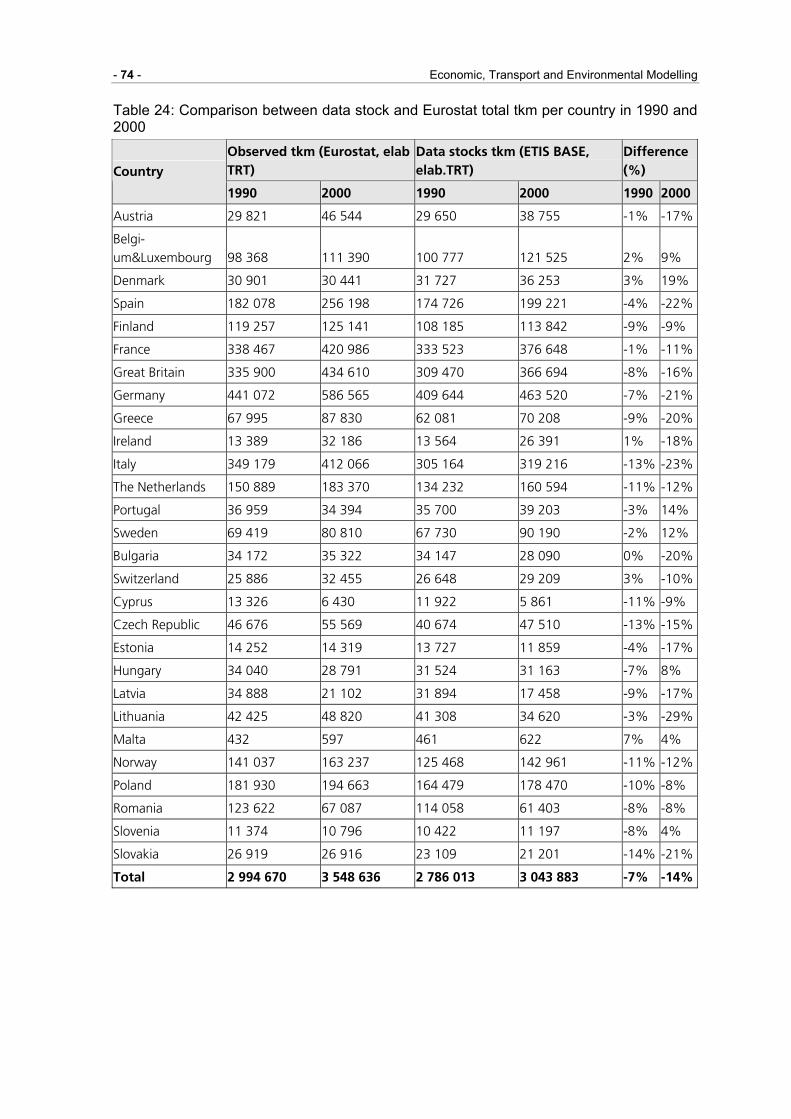
- 74 - Economic, Transport and Environmental Modelling
Table 24: Comparison between data stock and Eurostat total tkm per country in 1990 and 2000
Observed tkm (Eurostat, elab TRT)
Data stocks tkm (ETIS BASE, elab.TRT)
Difference (%) Country
1990 2000 1990 2000 1990 2000
Austria 29 821 46 544 29 650 38 755 -1% -17%
Belgi-um&Luxembourg 98 368 111 390 100 777 121 525 2% 9%
Denmark 30 901 30 441 31 727 36 253 3% 19%
Spain 182 078 256 198 174 726 199 221 -4% -22%
Finland 119 257 125 141 108 185 113 842 -9% -9%
France 338 467 420 986 333 523 376 648 -1% -11%
Great Britain 335 900 434 610 309 470 366 694 -8% -16%
Germany 441 072 586 565 409 644 463 520 -7% -21%
Greece 67 995 87 830 62 081 70 208 -9% -20%
Ireland 13 389 32 186 13 564 26 391 1% -18%
Italy 349 179 412 066 305 164 319 216 -13% -23%
The Netherlands 150 889 183 370 134 232 160 594 -11% -12%
Portugal 36 959 34 394 35 700 39 203 -3% 14%
Sweden 69 419 80 810 67 730 90 190 -2% 12%
Bulgaria 34 172 35 322 34 147 28 090 0% -20%
Switzerland 25 886 32 455 26 648 29 209 3% -10%
Cyprus 13 326 6 430 11 922 5 861 -11% -9%
Czech Republic 46 676 55 569 40 674 47 510 -13% -15%
Estonia 14 252 14 319 13 727 11 859 -4% -17%
Hungary 34 040 28 791 31 524 31 163 -7% 8%
Latvia 34 888 21 102 31 894 17 458 -9% -17%
Lithuania 42 425 48 820 41 308 34 620 -3% -29%
Malta 432 597 461 622 7% 4%
Norway 141 037 163 237 125 468 142 961 -11% -12%
Poland 181 930 194 663 164 479 178 470 -10% -8%
Romania 123 622 67 087 114 058 61 403 -8% -8%
Slovenia 11 374 10 796 10 422 11 197 -8% 4%
Slovakia 26 919 26 916 23 109 21 201 -14% -21%
Total 2 994 670 3 548 636 2 786 013 3 043 883 -7% -14%

TRIAS D3 Outlook for Global Transport and Energy Demand - 75 -
4.1.3.5 Regional Economics Module
The revision of Regional Economic module concerned the update of the trip rates for NMS
countries, which were previously calculated in a simplified way due to lack of information.
Trip rates differentiated into age groups, employment situation and car-availability represent
the average mobility behaviour of specific groups of population. In the passenger trip genera-
tion stage in the ASTRA Regional Economic model (REM) they are applied to calculate the
passenger trips per country and population groups. Most Western European countries and
members of EU15 frequently performed mobility or travel surveys among the population
helping to identify mobility patterns of specific population clusters, like for example the Ger-
man and the Dutch mobility survey or the UK travel survey. Analysing and comparing these
mobility surveys lead to the insight that mobility patterns and average numbers of trips per
person in these countries resemble one another. Country-specific GDP per capita numbers
from EUROSTAT show that the values for the year 2000 are also similar and in a range be-
tween 25,000 and 26,500 Euro per inhabitant.
In contrast to the various information on trip rates provided by these and many other West-
ern European mobility surveys, no surveys were available for the New Member States of the
EU25 and the Candidate Countries Bulgaria and Romania. This lack of information and data
required the development of an appropriate methodology to estimate the passenger trip
rates in the New Member States. Unfortunately, no available transport database releases total
numbers of passenger trips for these countries. Only the passenger transport performance
measured in passenger-km can be found in databases like the “Energy & Transport in Fig-
ures” pocketbook published by the European Commission each year. This country-specific
transport performance indicator could serve as basic for the estimation of trip rates. In prac-
tise a transfer from pkm into passenger trips would require an estimation of average length
of trips differing from country to country depending on country-specific settlement patterns,
the location of workplaces and other indicators. Therefore an alternative methodology has
been chosen to estimate the passenger trip rates in the New Member States.
According to the differentiation of trip rates in EU15 countries the country-specific trips per
person and day are distinguished between the trip purposes business, private and tourism.
The UK travel survey provides the reference values per person and day for all three purposes.
In the year 2000 a person in the UK made on average about 2.5 business trips per day, 1.85
private trips per day and 25 holiday trips (trips of more than 2 days) per year. Furthermore
the GDP per capita for the initial year 1990 has been taken from EUROSTAT. The following
equation describes the chosen methodology for estimating the average number of trips per
person per day with trip purpose in the Eastern European countries.
GBR
iTPTPGBRTPTPi GDPpC
GDPpCATATATAT *)min(min ,, −+= (eq. 2)
where: ATi,TP = Average number of trips per person per day with trip purpose TP in country i min ATTP = Minimum average number of trips per person per day for trip purpose TP ATGBR,TP = Average number of trips per person per day with trip purpose TP in the UK GDPpCi = Gross Domestic Product per Capita in country i GDPpCGBR = Gross Domestic Product per Capita in the UK

- 76 - Economic, Transport and Environmental Modelling
The computation requires the assumption of a minimum number of trips per person and trip
purpose per day. This assumption has been performed by determining a minimum number of
average trips per person and year of about 800 trips compared to 1021 in the UK. The as-
sumption of business trips being more essential than private or holiday trips and people with
lower incomes have to save money by reducing the number of holiday and private trips re-
sulted in the following minimum number of trips per person: 2.3 business trips, 1.5 private
trips and 4 holiday trips.
In comparison with the trip rates for EU15 the resulting trip rates for the Eastern European
New Member States of EU25 are only disaggregated into three trip purposes and do not con-
sider employment or car-availability. The EU15 passenger trip generation model was originally
based on trip rates per age segment, employment status, car-availability and trip purpose
taken from SCENES. As these trip rates did not distinguish between different mobility pat-
terns from country to country a special calibration was implemented in ASTRA. The country-
specific differences were taken into account by calibrating the trip rates to fit the total num-
bers of trips per purpose and functional zone in a country. For the estimation of Eastern
European trip rates the same approach was applied.
Hence, in the approach the total number of trips per country in a year was computed out of
the number of average trips per person and trip purposes by applying employment and
population numbers for the initial year 1990 taken from EUROSTAT. The total number of
business trips was calculated by assuming an average of 260 working days per year and mul-
tiplying them with the employment numbers and trip rates. For the computation of yearly
private and holiday trips the whole population was considered. Splitting the trips per country
and trip purpose into the functional zones by taking into account the share of population
living in the zone enabled the recalculation of country-specific trip rates originally taken from
SCENES.
One major assumption behind the trip generation based on trip rates in ASTRA is that trip
rates are fixed over time for homogenous segments of populations. Notwithstanding, the trip
rates for the New Member States have been increased over the calibration period. This is jus-
tified because of the rougher segmentation of individuals available for such countries when
compared to the EU15. Employed people and who own a car make more trips and both such
groups are expected to increase in the future in the New Member States. Therefore it is ex-
pected that trip rates in such countries will tend to become more similar to those in the
EU15.
4.1.3.6 Infrastructure Module
The revision of the infrastructure capacity structure included two different activities, as fol-
lows:
• Testing different parameters for current flow/capacity functions to emphasize the role
of congestion;
• Testing and calibrating a different structure for implementing congestion effects.

TRIAS D3 Outlook for Global Transport and Energy Demand - 77 -
Testing Different Parameters for Current Flow / Capacity Functions to Emphasize the Role of Congestion.
The parameters of the flow/capacity functions of the different modes have been tested in
order to emphasise the role of the congestion. After several tests, road function has been
made steeper in the first part of the function, when the flow/capacity ratio is lower than 1.
The intervention has been stronger at local level and weaker for long distance network. The
changes allowed the model to simulate a slight reduction of the road modal shares (car and
bus) as the occupancy of capacity grows, with correspondent increase of slow trips at local
level and rail and air for long distances.
A revision has been done also on rail, air and ship flow/capacity functions in order to prevent
non-road modes to increase rapidly their share even when the estimated capacity is reached.
New parameters have been set for air and ship while the parameters for rail rested un-
changed.
During the tests, some questionable data concerning capacity has been detected. For rail and
road alternative values have been estimated and included in the model.
Testing and Calibrating a Different Structure for Implementing Congestion Effects
The original objective of this task was twofold. On the one side, it was planned to test
whether steeper speed-flow functions would give rise to model oscillations when congestion
appear and, in such a case, to implement a different structure to “smooth” travel time. Sec-
ondly, a new structure has been implemented, splitting infrastructure into a congested and
non-congested part for which the shares are provided from VACLAV. The non-congested
part is related to the base time per km, while the congested part is related to the time per km
resulting from the application of the speed-flow curve or – in case an iterative interaction
with VACLAV is implemented – directly by output of the VACLAV network model.
4.1.3.7 Vehicle Fleet Module
The previous version of the ASTRA vehicle fleet module (VFT) consisted of four separate
models representing the passenger car, bus, light duty vehicle (LDV) and heavy duty vehicle
(HDV) fleets in EU27+2 (EU27 plus Norway and Switzerland). The major indicator simulated
by each of the four models is the number of vehicles in each country for the simulation pe-
riod. There is a common structure implemented, which is characterised by a feedback be-
tween new vehicle purchases per year, the number of vehicles per age class, the scrapping of
vehicles per year and a generated demand regulating the change of vehicle fleets and the
replacement of scrapped cars and therefore the new registered vehicles per year.
In contrast to the ASTRA bus and HDV model, the passenger car and LDV model differentiate
between diesel and gasoline driven motors. Furthermore the previous version of the car fleet
model distinguished between three different cubic size groups for gasoline driven cars and
two groups for diesel driven cars. All previous models differentiate emission categories
(ece1503 until Euro5) determined by their date of purchase in common. The above-
mentioned demand driving the change of fleet by new registrations is implemented in a dif-

- 78 - Economic, Transport and Environmental Modelling
ferent way in the four models. Bus, LDV and HDV new registrations are induced by vehicle-
kilometre driven in the respective freight transport model. For instance LDV registrations are
modelled to be dependent on vehicle-kilometres driven in local, regional and medium dis-
tance bands, while HDV registrations depend on longer distance vehicle-kilometres driven.
The major objectives of TRIAS, to analyse the impacts of supporting hydrogen and biofuel
technologies, required a significant revision of the previous passenger car fleet model. In or-
der to simulate the potentials of hydrogen and biofuels as prospective vehicle technologies
IWW expanded the passenger car model with six new car technologies. Figure 34 highlights
the six new alternative car technologies besides the five already existing conventional car
categories. Hybrid cars (HYB) comprise a combination of combustion and electric motors. The
revised model does not distinguish between hybrid cars equipped with diesel respective gaso-
line motors. An exogenous share is estimated to assign the emissions and fuel consumption
to diesel respective gasoline technology. As many contemporary conventional diesel cars al-
low driving with biodiesel the new car category bioethanol cars (BIO) does only contain cars
driving with bioethanol E85. Finally, the new category hydrogen cars (H2) is implemented
and incorporates fuel cell cars as well as cars with direct combustion engines. Regarding the
current low frequency of filling stations offering alternative fuels the automotive industry
developed many alternative fuel cars that can be driven by conventional fuels as well. The
revised car fleet model allocates these hybrid car categories to the alternative fuel categories
and not to the conventional car categories.
Astra Car Categories (CC)
Conventional Alternative
• GPC1 (Gasoline < 1.4 l)
• GPC2 (Gasoline > 1.4 l ∧ < 2.0 l)
• GPC3 (Gasoline > 2.0 l)
• DPC1 (Diesel < 2.0l)
• DPC2 (Diesel > 2.0 l)
• CNG (Compressed Natural Gas)
• LPG (Liquified Petroleum Gas)
• HYB (Hybrid)
• ELC (Electric Current)
• BIO (Bioethanol E85)
• H2 (Hydrogen)
Figure 34: New ASTRA passenger car categories
The purchase decision for one of the five conventional car categories in the previous ASTRA
car fleet model was driven by aggregated factors like differences between gasoline and diesel
fuel prices, different taxation and a factor representing fashion. In order to integrate the new
alternative car technologies IWW identified the major drivers of people that decided to buy a
new car. Several US studies and the most recent ARAL (2005) study elaborated via costumer
surveys potential factors influencing the decision of a car purchaser for a certain car respec-
tive car technology. In the following the European study from Aral is focused, as the new
purchase decision model simulates the EU27+2 markets. Figure 35 gives a detailed overview
on the survey. According to this study the costumers set a high value on economic efficiency

TRIAS D3 Outlook for Global Transport and Energy Demand - 79 -
for new cars. Price in combination with the provided performance of a car is the most signifi-
cant factor with 55% followed by the mileage of the car. Compared with older surveys the
factor safety lost significance but ,nevertheless, safety still plays an important role for 47% of
all interviewed customers. Besides economic and technical factors influencing the car pur-
chase decision the study included also soft factors like design, image and prestige. In contrast
to the economic factors they are supposed to be not as important. The low importance of
factors like the environmental-friendly-ness of a new car indicates that alternative fuel cars
can only diffuse successfully into the European markets when they can be purchased and
operated for an adequate price.
Based on the cognitions of this survey and the feasibility to quantify drivers in a System Dy-
namics model the revised car fleet model concentrates on the economic efficiency as major
impact for the purchase decision.
Drivers of Car Purchase Decision
0% 10% 20% 30% 40% 50% 60%
Image/Prestige
Flexibility
Family-friendly
Eco-friendly
Capacity
Ergonomics
Space
Resale Value
Price
Comfort
Design
Safety
Mileage
Price-Performance
Source: Aral Study (2005)
Figure 35: Drivers of Car Purchase Decision
Due to the characteristics of the purchase as a discrete choice for one out of eleven car cate-
gories respective technologies a logit-model was supposed to be the most sophisticated ap-
proach for simulating this decision. The implemented logit-function requires specific user
benefits of all eleven car technologies that can be chosen. Similar to the application of logit-
functions in the modal-split transport modelling stage this model does not compute benefits
but costs that can be put into the logit-function as negative benefits according to the follow-
ing equation.

- 80 - Economic, Transport and Environmental Modelling
∑ +−+−
=
CCECCCECCCEC
ECCCECCCECECCC LCpC
LCpCP
)*exp()*exp(
,,
,,, λ
λ (eq. 3)
where: PCC,EC = share of purchased cars per car category CC and country EC pCCC,EC = perceived total costs per vehicle-km per car category and country EC λEC = multiplier lambda per country EC LCCC,EC = logit const per car category CC and country EC representing the disutility CC =eleven car categories/technologies EC =EU27 plus Norway and Switzerland
The revised car fleet model calculates the required average costs per vehicle-km for each car
category in a bottom-up approach. On the one hand the model computes variable costs per
vehicle-km based on average fuel consumption factors for each technology and country-
specific fuel prices provided by POLES. Fuel consumption factors for conventional cars are
derived from Umweltbundesamt (2004)7. Available sales figures for specific car types for each
alternative car category and general information from OEMs are used to generate average
fuel consumption factors for the six new car categories.
Besides variable costs the model considers also fixed costs for each car category. Detailed car-
ownership taxation, registration fees and purchase costs per country and car category and
country-specific average maintenance costs determine the fixed costs per car category and
country. All elements of fixed costs are transformed into costs per vehicle-km by dividing
through average yearly mileages per car category and country. Average values for yearly
mileages are based on car passenger-km and car-ownership taken from EU Energy and Trans-
port in Figures 2005 and average occupancy rates taken from the TRANSTOOLS model. As
the conversion of purchase costs into costs per vehicle-km requires information on average
lifetime per car category the average lifetime per car category and country is derived from the
car stock cohort model via feedback loop. Similar to the approach for computing of average
fuel consumption factors for alternative fuel cars, average purchase costs for alternative fuel
cars are performed considering sales figures from the last years.
Assuming completely rational purchase decision behaviour based on all variable and fixed
costs would disregard other important drivers like the distribution grid of filling stations sell-
ing the requested type of fuel. For conventional fuel types like gasoline and diesel the distri-
bution grid is characterised by a good quality in all EU27+2 countries. At present, owners or
prospective costumers of alternative fuel cars have to cope with the burden that the pro-
curement of alternative fuels requires significantly longer additional trips or is even not feasi-
ble due to lacking filling stations. JANSSEN (2004) concluded in his paper on CNG market
penetration that successful diffusion of new car technologies depend on a uniform develop-
ment of technology and filling station infrastructure. Against the background of these signifi-
cant impacts due to fuel supply differences the model has to consider the quality of filing
station grids as well. Hence, the four mentioned cost categories have to be completed by so-
called fuel procurement costs.
7 Umweltbundesamt (2004): Handbook Emission Factors for Road Transport, Version 2.1

TRIAS D3 Outlook for Global Transport and Energy Demand - 81 -
In order to generate these costs per vehicle-km for each car category and country the model
requires input in terms of filling station numbers for each fuel category diesel, gasoline, LPG,
CNG, electric current, E85 and hydrogen. Conventional filling stations are derived from na-
tional statistics offices and automobile associations, alternative fuel filling station numbers
were taken from European Natural Gas Vehicle Association8 and other databases9. Due to
lacking information about the spatial distribution of filling stations the revised model assumes
a homogenous distribution. This leads to an average surface area for each fuel category that
have to be served per filling station. The model considers the optimisation efforts of mineral
oil groups in locating new filling stations efficiently by assuming a central location in a unit
circle representing the average surface area. In order to calculate an average distance that
has to be driven for refuelling a car three situations for the car-owner are conceivable:
• refuelling requires no extra trip because the filling station is located on the way to
another destination
• refuelling requires an extra trip for the car-owner starting in an area near the filling
station (25% of maximum distance)
• refuelling requires an extra trip for the car-owner starting in an area far away from
the filling station (75% of maximum distance)
x
Dmax
75% Dmax
25% Dmax
x
Dmax
75% Dmax
25% Dmax
Figure 36: Estimation of average distance to filling station
Weighting the option without extra-trip by 25%, the situation near by 50% and the far away
option by 25% the model simulates an average trip distance for each refuelling action. Aver-
age cruising ranges per car category allow the calculation of total yearly kilometre that have
to be driven for refuelling a car with a certain technology. Finally the model simulates the fuel
procurement costs by multiplying the yearly km with fixed and variable costs per vehicle-km
and adding the opportunity costs generated via value of time and required time for the pro-
curement trips extracted from the ASTRA transport module (TRA).
The following equation describes the simulation of perceived total car costs per vehicle-km
that are composed of variable/fuel, purchase, taxation, maintenance and fuel procurement
costs. Furthermore the model considers the importance of purchase cost level for the calcula-
tion of perceived costs by setting a car category and country- specific weighting factor.
8 European Natural Gas Vehicle Association (ENGVA): http://engva.org 9 http://www.gas-tankstellen.de, http://www.erdgasfahrzeug-forum.de, http://www.h2stations.org

- 82 - Economic, Transport and Environmental Modelling
ECCCECCCECECCCECCCECCCECCC procCvCmCtaxCpCC ,,,,,, * ++++=α (eq. 4)
where: CCC,EC =perceived car cost per vehicle-km per car category CC and country EC pCCC,EC =purchase cost per vehicle-km per car category CC and country EC taxCCC,EC =taxation/registration cost per vehicle-km per car category CC and country EC mCEC = maintenance cost per vehicle-km per country EC vCCC,EC = variable/fuel cost per vehicle-km per car category CC and country EC procCCC,EC = fuel procurement cost per vehicle-km per car category CC and country EC αCC,EC =weighting factor representing the significance of purchase costs CC =eleven car categories/technologies EC =EU27 plus Norway and Switzerland
Finally the logit function simulates the probability of cars purchased for each of the eleven
technologies based on the simulated perceived car costs. Figure 37 gives an overview on the
implemented approach for simulating the share of each technology on total cars registered.
In the process of calibration an optimal set of parameters could be identified for the weight-
ing factor α, logit parameter λ and the logit const LC. IWW calibrated all parameters with the
Vensim™ internal optimisation tool. Time series data for car registration per country disag-
gregated into car categories was taken from EUROSTAT online database10. Several lacking
datasets, especially for alternative fuel car registrations, required further data sources like
data from ACEA11 and further data sources.
10 EUROSTAT online database: http://epp.eurostat.cec.eu.int 11 European Automobile Manufacturers Association (ACEA): http://www.acea.be

TRIAS D3 Outlook for Global Transport and Energy Demand - 83 -
Costs per vkm
FC Factors
FuelCosts MaintenanceTaxation Mileage Car
Prices Lifetime
Variable Costs
InvestementCosts
FillingStations
Land Area VoT Timekm FC
FactorsTank Size Mileage
Total Costsper vkm
Fixed Costs
Ø Distance to FS
ProcurementCosts per vkm
ProcurementCosts
FeedbackPOLESENV.car
POP TRA ENV.car
Share New Cars per CC
Weight
Weight
Weight
Logit Costs per vkm
FC Factors
FuelCosts MaintenanceTaxation Mileage Car
Prices Lifetime
Variable Costs
InvestementCosts
FillingStations
Land Area VoT Timekm FC
FactorsTank Size Mileage
Total Costsper vkm
Fixed Costs
Ø Distance to FS
ProcurementCosts per vkm
ProcurementCosts
FeedbackPOLESENV.car
POP TRA ENV.car
Share New Cars per CC
Weight
Weight
Weight
Logit
Figure 37: ASTRA car purchase model
After simulating the share of new cars per car category with the new car purchase model this
share is multiplied with the total number of new car registered per country. Figure 38 dem-
onstrates the implemented feedback loop in the car fleet model. Starting with an initial share
of cars per car category, emission standard, country and age for each simulation period the
new purchased cars are added while all scrapped cars in the different age cohorts are sub-
tracted by the model. The number of scrapped cars is one of the drivers of total new regis-
tered cars per year as the model assumes that a certain share of all scrapped cars are re-

- 84 - Economic, Transport and Environmental Modelling
placed by new ones. Furthermore new registrations per year are assumed to be dependent
on the development of variable costs for operating a car, population, population density,
average car prices, the level of motorisation and the average income per adult. Population
density as a representative for urbanisation, car price, fuel prices and the level of motorisation
dampen new registrations while income per adult and population increase new registrations.
Car_Fleet_CCESPurchase_Cars_CC_ES Car_Scrappage_CC_ES
Registration_New_CarsTotal Minimum_Replacement_Cars
+
Car_Fleet_Total
+
+
Car_Scrappage_Total
+
+
Delta_Income_per_AdultDelta_PopulationDelta_Variable_Costs
- ++
New_Cars_CC+
Share_New_Cars_CC
New_Cars_CC_ES
+
+
Diffusion_New_ES
+
Car_Ownership
+
-
Consumption_for_New_Cars
Car_Scrappage_Ratio
+
+
Car_Prices_CC_ES
+
Input MAC_con
Input ENV_car
Output POP
Output MAC_con
Delta_Car_Prices -
Output POLES
+
Delta_Population_Density
+
Technology Share
Figure 38: ASTRA car fleet model
Figure 39 illustrates a representative result and highlights the dynamic modelling of emission
standards in the car fleet model. The figure demonstrates the development of diesel car stock
per emission category in Germany from 1990 to 2050. The total number of diesel cars with
cubic capacities less than 2.0 litre is increasing significantly until the year 2035. All other
curves represent the life-cycle dynamics of emission standards until the projected Euro7 cate-
gory. New purchased cars after the year 2020 fulfil per definition the Euro7 standard. Caused
by the small intervals between the introduction of new emission standards in Europe the life-
cycle curves are characterized by strong growth in the first years and a continuous decrease
when the new standards enter the market.

TRIAS D3 Outlook for Global Transport and Energy Demand - 85 -
ASTRA car fleet life cycle - Example GER Diesel < 2.0 l
0
4
8
12
16
20
24
28
32
1990
1994
1998
2002
2006
2010
2014
2018
2022
2026
2030
2034
2038
2042
2046
2050
[Ths
car
s]
ece1504Euro1Euro2Euro3Euro4Euro5Euro6Euro7Total
Figure 39: Example for car life cycle modelling in ASTRA VFT module
Finally, the model disaggregates the new cars into car categories respective technologies via
the share generated in the car purchase model. Based on pre-defined diffusion years for all
modelled emission categories the number of new cars per car category and country are as-
signed to the respective emission standards. In the ASTRA model the following diffusion
years respective periods are implemented: Table 25 shows all emission standards and their
assumed diffusion time respective period. In contrast to the previous version of the ASTRA
vehicle fleet model the new version includes Euro 6 and Euro 7 emission standards. Accord-
ing to the European Parliament (T6-0561/2006) 2014 was proposed as year of introduction
for Euro 6. Based on the average interval between the introduction of two emission catego-
ries, IWW decided to diffuse Euro 7 standard cars in the year 2020. The new emission stan-
dards Euro 6 and Euro 7 were integrated as well in the bus, light duty and heavy duty vehicle
models with the same chronological schedule as in the car fleet model.
Table 25: Diffusion of emission standards in ASTRA Emission Standard Diffusion Year/Period
ece1503 before 1990ece1504 before 1990Euro 1 1991 until 1992Euro 2 1994 until 1996Euro 3 1998 until 2000Euro 4 2004 until 2005Euro 5 2007 until 2008Euro 6 2012 until 2014Euro 7 2018 until 2020
Source: ASTRA (2007)

- 86 - Economic, Transport and Environmental Modelling
Similar to the car purchase model the car fleet model is calibrated based on EUROSTAT car
fleet and aggregated new registration data. The calibration tool in Vensim™ optimises
weighting factors for all mentioned drivers of new car registration plus the vehicle-age-
specific scrapping factors. According to observed historical correlations and results of the
optimisation the demographic development, changes in income per adult and variable cost
changes prove to be the most important drivers of motorisation.
4.1.3.8 Environmental Module Improvements
The main objective of the ASTRA environmental module (ENV) is the computation of trans-
port related emissions, fuel consumption and accidents. The significant improvements im-
plemented in the other modules of ASTRA for the TRIAS project, especially the expansion of
the vehicle fleet module with new alternative car technologies required an update of the pre-
vious ENV module. Furthermore the module had to be revised in order to take into account
the new emission standards Euro 6 and Euro 7.
The ASTRA ENV module generates CO2, CO, NOx, VOC and soot particles emissions for all
transport modes. In order to represent the whole life-cycle of transport related emissions, hot
emissions, cold start emissions, vehicle production emissions and fuel production emissions
are considered. Hot and cold start emissions are simulated on the basis of emission factors
per car category, emission standard and, only for hot emissions, different traffic situations
taken from HBEFA12. The model is able to generate hot emissions for each pollutant via
mode-specific transport performance in vehicle-kilometres-travelled provided by the TRA
module. The number of trips per mode acts as input for the computation of cold start emis-
sions.
As POLES requires according to the TRIAS interface approach fuel demand in terms of fuel
consumption per type of fuel all alternative fuel categories were implemented in the ENV car
module. Additionally the averaged passenger car fuel consumption necessary for calculating
the variable cost development in the modal split was updated and extended by the new fuel
categories.
4.1.4 Implementation of Baseline and Reference Scenario
This section explains major assumptions that have been made in ASTRA to implement the
baseline scenario. To make data consistent between the different models or when data
comes from different statistics an agreed set of deflators to convert into constant EURO
prices for the year 1995 are applied (see Table 26).
Table 26: Applied deflators to harmonize data between models 1990 1991 1992 1993 1994 1995 1996 1997 1998
GDP-Deflator Euro 1995 1.1993 1.1438 1.0962 1.0578 1.0289 1 0.9791 0.9640 0.9477
12 Handbook of Emission Factors, HBEFA version 2.1 (2004)

TRIAS D3 Outlook for Global Transport and Energy Demand - 87 -
1999 2000 2001 2002 2003 2004 2005 2006 2007 GDP-Deflator Euro 1995 0.9372 0.9252 0.9026 0.8795 0.8598 0.8418 0.8261 0.8101 0.7928
Source: EUROSTAT online database
4.1.4.1 MAC Assumptions
For the exogenous parameters of the macroeconomics module the same assumptions as in
previous studies are applied (e.g. Schade 2005) and are extended from 2025 until 2050 with
their value of 2025. For a number of exogenous trends this constitutes an optimistic picture.
E.g. the annual growth rates of labour productivity are taken as constant after the year 2025.
An alternative and also reasonable assumption would have been to assume decreasing
growth rates because both potentials for productivity increases diminish over time and the
assumption of constant absolute productivity increase is applied in other projects, which im-
plies to use continuously decreasing annual growth rates.
4.1.4.2 FOT Assumptions
A major assumption affecting the trade model of ASTRA concerns the GDP development in
regions of countries outside Europe i.e. outside the EU29 countries considered in ASTRA.
Assumptions for these trends were taken from the ADAM baseline (EU 6FP project). How-
ever, since in past projects a clear cyclical behaviour of these trends was observed the ADAM
trends were overlayed with a cyclical behaviour to shape the final exogenous GDP growth
trends to be applied in ASTRA. These trends are shown in Figure 40.
D a t a a n d e x o g e n o u s g r o w t h t r e n d s o f G D P o f R o W - r e g i o n s ( a n n u a l p e r c e n t a g e c h a n g e )
- 1 0
- 5
0
5
1 0
1 5
2 0
1 9 9 0 1 9 9 4 1 9 9 8 2 0 0 2 2 0 0 6 2 0 1 0 2 0 1 4 2 0 1 8 2 0 2 2 2 0 2 6 2 0 3 0 2 0 3 4 2 0 3 8 2 0 4 2 2 0 4 6 2 0 5 0
W o r ld
O z e a n ia
C h in a
E a s t A s ia
In d ia
J a p a n
L a t in A m e r ic a
N o r t h A m e r ic a
T u r k e y
R e s t - o f - t h e - w o r ld
Figure 40: Exogenous GDP growth trends of rest-of-the-world regions in ASTRA
4.1.4.3 TRA Assumptions
As far as the transport module is concerned, the implementation of the reference and base-
line scenarios consists in the definition of the how travel costs develop over the future time
horizon. The TRIAS baseline and reference scenarios do not differ to each other for assump-

- 88 - Economic, Transport and Environmental Modelling
tions concerning the transport side. Therefore for the TRA module, the two scenarios are
identical.
Part of the cost items used in the TRA module develop endogenously as effect of either other
components of the ASTRA model (e.g. the vehicle fleet) or of the interaction with the POLES
model (e.g. the pure fuel prices). In such a cases, the use of exogenous trends has been
avoided and the endogenous trends are taken. For the other cost items, the assumptions
made in the ASSESS project (Mid Term assessment of the European Commission white paper,
see De Ceuster et. al., 2005) have been considered, namely the assumption of the partial B
scenario (see Martens et. al., 2005).
In brief, in ASSESS for the passenger modes, the effect of future policies implementation is
supposed to keep user costs constant, with exclusion of train where a slight reduction is ex-
pected. For the freight modes, the policy measures considered in the ASSESS scenario are
expected to give rise to, sometimes significant, changes of transport costs. However, one the
one side the ASSESS measures are still largely unapplied and on the other side they concern
taxation and pricing measures which could be at least partially overlapping with the carbon
tax envisaged in the TRIAS scenarios. Therefore, as the TRIAS scenarios are not concerned
with the level of application of transport policy and its effects, it has been decided to avoid
the implementation of cost changes which, on the one side, could alter the relative competi-
tiveness of transport modes even if this does not seem the current baseline trend and, on the
other side could make confusion when the TRIAS scenarios are implemented.
One exogenous assumptions included in the TRA freight model is that the road haulage sec-
tor become more efficient as the amount of transported goods increases. When there are
more trades between countries, more goods to be locally distributed, etc. it is easier to opti-
mise the vehicle loads, avoiding empty trips, etc. Furthermore, the growth of fuel price
prompts carriers to improve efficiency. This is translated in the model by means of increasing
load factors. The impact of higher load factors is to lower costs per ton-km of road freight.
The following table summarizes the trend of total transport cost per km by mode (passenger
and freight) under the assumption considered for the Baseline scenario from 2000 to 2050.
The changes in the table are final output of the models in terms of weighted average, so
include the evolution of the matrix, of the load factors, etc. This is the reason why even
modes for which no specific exogenous changes have been implemented change their costs
and, at the same time, the effect on modes where inputs have been implemented is not the
mere reproduction of the input.
It can be noticed that car cost per pass-km is supposed to rise as effect of fuel price. Instead
road freight cost per ton-km is supposed to diminish because the increment of fuel price
(which is just a share of total road freight cost) is more than off-set by the higher load fac-
tors.

TRIAS D3 Outlook for Global Transport and Energy Demand - 89 -
Table 27: Trend of total transport cost by mode (passenger and freight) Averaged cost 2000 2010 2020 2030 2040 2050
Passenger averaged cost per pkm
Car 100 140 122 112 123 142
EU15 Bus 100 102 101 100 99 100
Train 100 100 100 101 101 101
Air 100 107 104 102 106 114
Car 100 102 93 93 103 114
EU12 Bus 100 100 101 101 102 102
Train 100 99 97 95 94 92
Air 100 111 106 104 107 113
Freight averaged cost per tkm
Road 100 101 98 95 95 95
EU15 Rail 100 106 109 110 111 113
Ship 100 104 104 105 106 107
Road 100 89 83 80 81 82
NMS Rail 100 104 103 102 101 100
Ship 100 100 103 107 113 117
The following graphs summarise the base trend of the passenger and freight traffic in the
baseline scenario. For a more detailed analysis see section 3. The trend of personal mobility
shows an increment at different speed when EU15 and more recent EU Member States are
considered. The latter are forecasted to grow faster in the near future as impact of higher
incomes and motorisation rates. However, the expected decreasing population in the Eastern
Europe countries partially offsets these determinants resulting in a diminished growth rates
and finally also in a reduced mobility in absolute terms. The difference between the two
groups of countries is more significant looking at the mobility of goods, which in the Eastern
Europe countries is expected to increase more significantly due to the higher economic de-
velopment rates.

- 90 - Economic, Transport and Environmental Modelling
Total passenger traffic index (year 2000 = 100)
0
20
40
60
80
100
120
140
160
180
2000
2002
2004
2006
2008
2010
2012
2014
2016
2018
2020
2022
2024
2026
2028
2030
2032
2034
2036
2038
2040
2042
2044
2046
2048
2050
EU15 EU12
Figure 41: Baseline trend of total pkm
Total freight traffic index (year 2000 = 100)
0
50
100
150
200
250
300
350
400
450
500
2000 2005 2010 2015 2020 2025 2030 2035 2040 2045 2050
EU15 EU12
Figure 42: Baseline trend of total tkm
4.1.4.4 REM Assumptions
The REM module uses endogenous input from other model components (population, motori-
zation rate, GDP, intra-EU trade, etc.) Therefore, there is no need of specific assumptions to
implement the scenarios.

TRIAS D3 Outlook for Global Transport and Energy Demand - 91 -
4.1.4.5 INF Assumptions
No specific assumptions are required in the Infrastructure module to implement the baseline.
As far as travel times are derived from the VACLAV model, such a model includes in the fu-
ture network the new infrastructures assumed in the baseline scenario.
4.1.4.6 VFT Assumptions
Two categories of assumptions are implemented for the TRIAS reference and baseline sce-
nario in the vehicle fleet passenger car module: assumptions on prospective cost develop-
ment and general assumptions on penetration probability of alternative technologies.
Regarding the costs car-ownership respective car registration taxation is the one driver of the
car purchase model that is influenced by the assumptions. Taxation in the TRIAS reference
and baseline is assumed to stay on the last available country-specific level. Taxation rates and
fees are taken for each country for historical period from 1990 to 2006. The second cost
category that is impacted by the TRIAS assumptions is the development of car prices for each
of the modelled eleven car categories. Basic prices are taken from the year 1995 for the con-
ventional gasoline and diesel cars and from the year 2005 for alternative technologies. Table
28 displays the assumed car price development for each technology. Bioethanol and hydro-
gen car price assumptions were taken from the hydrogen and biofuels database developed
for TRIAS D1.
Table 28: Assumed car price development per technology
2020 2030 2050Conventional 25% 38% 44% CNG 13% 17% 20% Hybrid 13% 17% 20% Electric 13% 17% 20% Bioethanol 3% 0% -3% Hydrogen 0% -13% -26%
Car price developmentCar Technology
The third cost type that is estimated in its development is the so-called fuel procurement
costs. Fuel procurement costs are mainly influenced by the number of filling station offering a
certain fuel type. Table 29 presents the share of conventional filling stations offering hydro-
gen and bioethanol. This share is estimated by Fraunhofer ISI and University Karlsruhe (TH),
IWW.

- 92 - Economic, Transport and Environmental Modelling
Table 29: Assumed filling station infrastructure development for H2 and Bioethanol TRIAS scenario Country-Group 2020 2030 2040 2050
H2 First Movers 0.3% 2.2% 6.7% 20% H2 Slow Movers 0.1% 1.1% 3.3% 10% H2 First Movers 7% 18% 25% 25% H2 Slow Movers 3% 9% 14% 14% H2 First Movers 0.3% 2.8% 8.3% 25% H2 Slow Movers 0.1% 1.7% 5% 15%
Sweden 40% 50% 50% 50% BIO First Movers 28% 35% 35% 35% BIO Slow Movers 18% 25% 25% 25%
Sweden 50% 60% 60% 60% BIO First Movers 35% 40% 40% 40% BIO Slow Movers 25% 30% 30% 30%
All (besides BAU+REF)
First Mover
Carbon Tax + Subsidies
All (besides REF)
Carbon Tax + Subsidies
Finally the TRIAS partners decided to exclude certain technologies in the reference and base-
line scenario. Projects on behalf of the European Commission like HyWays13 shaped the ex-
perience that successful market penetration depends strongly on mechanisms that can pro-
vide incentives to car buyers purchasing a hydrogen driven car. Hence, hydrogen cars are
excluded by definition in the TRIAS baseline scenario, which should reflect a prospective
business-as-usual behaviour of systems in EU27. The diffusion of cars driven by bioethanol in
the EU27 market has already started in the last years. Based on this fact the model allows an
endogenous diffusion of bioethanol cars in the baseline scenario whereas the reference sce-
nario does not include bioethanol and hydrogen cars.
4.1.4.7 ENV Assumptions
According to the European Parliament the proposed emission limits for new cars documented
in T6-0561/200614 were adopted for the CO, NOx, VOC and soot particles hot emission fac-
tors for conventional cars and light duty vehicles for Euro 5 and Euro 6 in the baseline and
reference scenario. According to the European Parliament CO and VOC hot emission factors
remain on the same level for the emission standards Euro 4 to Euro 6. According to this
technological stagnation CO and VOC hot emission factors for the future Euro 7 standard are
as well assumed to stay on the same level. In contrast to these pollutants the proposed NOx
hot emission factors for Euro 5 standard decrease by -28% for diesel and –25% for gasoline
cars and for Euro 6 standard even by –55% for diesel while gasoline cars emission factors
remain on the Euro 5 level. Nevertheless, due to missing studies on expected prospective NOx
hot emission factors, the Euro 7 NOx hot emission factors in TRIAS are assumed to remain on
the Euro 6 level in the baseline and reference scenario.
The only pollutant that is not included in the proposal of emission limits is CO2. According to
the recent EU directive focussing the reduction of average CO2 emission factors for the vehi-
cle fleets of each automotive company a reduction of -15% CO2 from Euro 5 to Euro 6 and –
5% from Euro 6 to Euro 7 is implemented for conventional cars in the ENV module for the
baseline and reference scenario.
13 http://www.hyways.de/ 14 http://www.dieselnet.com/standards/eu/ld.php

TRIAS D3 Outlook for Global Transport and Energy Demand - 93 -
CNG cars hot emission factors implemented in the reference and baseline scenario are based
on OEM information from Opel and other OEMs offering CNG technology cars. According to
the automotive companies CO2 hot emissions can be reduced on average by –25% up to –
30% compared with average conventional gasoline cars. The improvement ranges for CO
hot emissions differ between –50% up to –90% reduction for CNG, while 85% up to 90%
of NOx hot emissions can be saved by CNG cars compared with average gasoline cars. VOC
and soot particle hot emissions can be reduced to a minimum such that these hot emissions
are assumed to be zero for CNG cars. Regarding the stated reduction ranges compared with
average gasoline cars, IWW estimated the CNG CO2, NOx and CO hot emission factors by
taking the average reduction rate and comparison with the emission factors of the gasoline
car category that has the highest share in EU27+2 car fleets: GPC2, gasoline cars between
1.4 and 2.0 litre cubic capacity.
Similar to CNG emission factors LPG hot emission factors could be derived from OEM infor-
mation for the baseline and reference scenario. Compared with an average gasoline car LPG
cars emit on average about –15% less CO2, -80% NOx, -80% CO and –60% VOC. Compa-
rable to CNG cars soot particle emissions could be minimised for LPG cars such that zero
emissions are assumed. Hybrid car hot emission factors could be calculated based on OEM
information for Toyota Prius, Honda Civic and Lexus. Bioethanol car hot emission factors
were taken from Volvo company information on flexifuel cars. Finally, the model assumes hot
emission factors for all pollutants for fuel cell respective direct hydrogen combustion cars and
electric cars to be zero. Emissions emerging in the fuel production process are considered in
the category fuel production emissions FPE. Country-specific average power plant emissions
are considered for electric current emissions.

- 94 - Economic, Transport and Environmental Modelling
Table 30: Assumptions on emission reductions after Euro 7 for baseline scenario
Year SourceCO warm Bus Diesel -1% -3% -5% 2025 Euro 7CO warm Car All -1% -3% -5% 2025 Euro 7CO warm HDV Diesel -2% -5% -8% 2025 Euro 7CO warm LDV All -1% -3% -5% 2025 Euro 7CO fuel production All Conventional -10% -18% -24% 1997 MEET D20CO2 warm Bus Diesel -3% -10% -15% 2025 Euro 7CO2 warm Car Gasoline -5% -15% -25% 2025 Euro 7CO2 warm Car Diesel -5% -10% -15% 2025 Euro 7CO2 warm Car Alternative -5% -10% -15% 2025 Euro 7CO2 warm HDV Diesel -5% -10% -15% 2025 Euro 7CO2 warm LDV Gasoline -10% -20% -30% 2025 Euro 7CO2 warm LDV Diesel -8% -15% -20% 2025 Euro 7CO2 fuel production All All -15% -20% -25% 1997 MEET D20NOx warm Bus Diesel -10% -20% -30% 2025 Euro 7NOx warm Car All -10% -25% -40% 2025 Euro 7NOx warm HDV Diesel -10% -20% -30% 2025 Euro 7NOx warm LDV All -5% -10% -15% 2025 Euro 7NOx fuel production All All -15% -20% -25% 1997 MEET D20PM warm Bus Diesel -10% -20% -30% 2025 Euro 7PM warm Car Diesel -5% -15% -25% 2025 Euro 7PM warm HDV Diesel -10% -20% -30% 2025 Euro 7PM warm LDV Diesel -5% -10% -15% 2025 Euro 7
VOC warm Bus Diesel -1% -3% -5% 2025 Euro 7VOC warm Car All -1% -3% -5% 2025 Euro 7VOC warm HDV Diesel -2% -5% -8% 2025 Euro 7VOC warm LDV All 0% 0% 0% 2025 Euro 7VOC fuel production All Conventional -10% -18% -24% 1997 MEET D20
Reduction based onPollutant Emissions Mode Fuel Type 2030 2040 2050
Source: ASTRA (2007)
Cold start emission factors for conventional cars were taken from handbook of emission fac-
tors (HBEFA, version 2.1). Emission factors projected for the year 2015 were implemented as
Euro 6 values, 2020 projections as Euro 7 projections.
Table 30 highlights the assumptions on emission reductions for all vehicles registered after
Euro 7. Furthermore fuel production emission reductions compared with the values gener-
ated in the MEET project are pictures in the following table for the baseline scenario.
TRIAS D3 Outlook for Global Transport and Energy Demand - 95 -
4.1.5 Modularisation of ASTRA
In order to further extend the functionality of the ASTRA model by a modelling team that is
spread across Europe a split into several independent modules was necessary. The necessity
of this task has been discussed in preceding projects. The growing model size became more
and more difficult to administrate in an environment with decentralised model development
taking place at three different locations in Europe. This was mainly because the model used
to be one huge file, and if two people made changes at the same time, these changes had to
be consolidated into one model in an extra, manual and time-consuming step.
The solution to this problem seemed to have been found in the tool Conductor, provided by
US colleagues of the Los Alamos National Laboratory presenting the Conductor at the System
Dynamics Conference 2006 in the Netherlands. At this occasion a workshop was hold and
the software was distributed to promote the usage of the Conductor. Use of the Conductor
would offer the possibility to separate ASTRA into various independent modules which could
be developed further independently by the different modelling teams, and automatically
merge these modules into one big file for running a simulation.
After a number of feasibility tests with the Conductor have been made successfully, the first
step to use the Conductor was to split ASTRA into separate Vensim model files. In order to
use the Conductor for merging the files, a set of rules and standards had to be applied dur-
ing the splitting of ASTRA. These rules were followed, but when the merging process was
tested with the full model, problems arose and the resulting model contained errors. In dis-
cussions with the developing team of the Conductor we confirmed that the errors did arise
due to specific features of ASTRA that would not be compatible with the version of the Con-
ductor tool, which we had at our disposition. Since, the Conductor is underlying quite strict
IPR rules in what concerns the distribution of the software code or of updates of the Conduc-
tor, it seemed impossible to find a joint solution within the time frame of the TRIAS project.
That fact led the TRIAS project team to the conclusion that the only sensible long-term solu-
tion for continued ASTRA model development would be the development of our own merg-
ing tool in order to be able to design the tool exactly to the ASTRA requirements and to
quickly react to the discovering of any errors. Therefore the TRIAS team decided to start de-
veloping our own tool, the ASTRA-merger written in Java. It was developed at Fraunhofer-ISI
and is distributed among all project partners along with a user manual.
After having split ASTRA into a set of modules, these have been put into a so-called version-
controlled repository, which can be accessed by every project partner via the internet. This
serves as the central storage place for the ASTRA model, so that all partners always work
with the same version of ASTRA. And due to the modularity it is possible that various people
work at the same time on different modules and thereby not disturb each other or overwrite
the partners’ work. Since having achieved the split into modules in early 2007 any further
development and improvement of ASTRA has taken place in the version controlled stand-
alone modules of ASTRA.

- 96 - Economic, Transport and Environmental Modelling
4.1.5.1 Model Structure – Modules and Associated Partner
For splitting ASTRA a two level nomenclature was developed. The first level is constituted by
9 modules, the second level by 35 models. ASTRA was then split into 35 models each being a
separate Vensim model file and each belonging to one of the 9 modules. All the variables
were given a prefix according to the module in which they are defined. This prefix is also
called namespace. Table 31 lists all modules and models along with the partner responsible
for its transformation for the ASTRA merger.
Table 31: List of modules and their associated models in ASTRA Sphere Module Model Partner Demography Population (POP) Pop.mdl IWW Economy Macroeconomics (MAC) MAC_con.mdl ISI MAC_emp.mdl ISI MAC_gdp.mdl ISI MAC_gov.mdl ISI MAC_inv.mdl ISI MAC_iot.mdl ISI WEM_mac.mdl ISI Foreign trade (FOT) FOT_agg.mdl ISI FOT_row.mdl ISI FOT_weu.mdl ISI WEM_fot.mdl ISI Transport Regional economics (REM) REM.mdl TRT Transport module (TRA) TRA_fre.mdl TRT TRA_pas.mdl TRT Infrastructure module (TRA) INF.mdl TRT Vehicle fleet module (VFT) VFT_bus.mdl IWW VFT_car.mdl IWW VFT_dev.mdl IWW VFT_hdv.mdl IWW VFT_ldv.mdl IWW Environment Environment module (ENV) ENV_acc.mdl IWW ENV_air.mdl IWW ENV_bus.mdl IWW ENV_car.mdl IWW ENV_dev.mdl IWW ENV_hdv.mdl IWW ENV_ind.mdl IWW ENV_ldv.mdl IWW ENV_rai.mdl IWW ENV_shp.mdl IWW WEM_dco.mdl IWW WEM_env.mdl IWW WEM_ext.mdl IWW WEM_int.mdl IWW Other Scenario settings SCE.mdl.mdl ISI Scenario iteration control Overview.mdl ISI

TRIAS D3 Outlook for Global Transport and Energy Demand - 97 -
4.1.5.2 ASTRA Merger
The ASTRA merger makes use of the possibility to store Vensim models as text files. It de-
composes each module to its elements and recompiles these elements into one valid model.
ASTRA merger was developed as an alternative to Conductor, since we needed the Conduc-
tor functionality, but the version provided to us was faulty, and no update could be obtained.
Since we started the splitting of ASTRA under the assumption that we will use Conductor for
the merging process, we used the Conductor criteria for the splitting into modules. Most of
them remained as criteria also valid for use with the ASTRA merger, some dispensable ones
were dropped, others remained in order to make the structure of the modules easier to ana-
lyse.
Technology
For the implementation of the ASTRA merger we choose Java 5. This decision was based on
various reasons:
• Java offers a very powerful programming library for finding patterns in text, so called
Regular Expressions. These are used for the decomposition of the individual modules
into their elements.
• Java is a high level programming language. This means that the application developer
does not need to take care of the implementation of low-level tasks like reading from
and writing to files.
• Java is optimised for the development of stable code. Performance was no criteria for
this task. This judgement was justified by the result. The complete ASTRA model is
compiled by the current version of the merger in less than half a minute.
• The responsible developer is experienced in the development of Java applications. He
made an assessment of other programming languages but judged Java as the best
available option and suggested this to the TRIAS project team.
Rules for modules
Modules have to follow these rules in order for the ASTRA merger to compile a valid Vensim
model out of the stand-alone modules, which are also running Vensim models:
• Hold a group of variables called in, the so-called interface variables. All variables in
this group are data-variables stored in a vdf data file. These are all the variables link-
ing the module to other modules receiving data from variables defined in other mod-
ules. This enables the module to be run as a stand-alone model. Variables in this
group have to be defined using the same subscript ranges as used in the definition of
that variable. E.g., if a subscripted variable is defined with two equations, using EU15
and EU12 subranges, then the '.in' group definition must use exactly this combina-
tion and not a single definition using a combined subscript range such as EU27.
• Underscores (or underbars as called by Vensim in dialog Tools/Options/Settings –
Show underbars) have to be activated so variable names do not contain white spaces.

- 98 - Economic, Transport and Environmental Modelling
• No space between variable name and subscript range, i.e.
VFT_Car_Fleet_per_EU_country[EUCoun]. This feature is provided by Vensim with the
Reform-and-Clean option.
• No colon: in variable names.
• No dot . in variable names.
• No <-> sequence in variable names.
• Formatting of in variables: grey and italic and defined as shadow variable to avoid un-
readable views after the merging process.
A number of special groups on the Vensim equation level is defined:
• Control,
• Global,
• Subscripts,
• Data,
• Venapp, and
• Policy.
These groups are merged and double defined variables are taken only once. This means that
we can have e.g. in the data group exactly the variables needed by the according module. If
another module also uses the same variable, then in the merged module the entry appears
only once.
It is possible to use the same name for groups in different modules. Vensim makes one group
of these by using the "reform and clean" feature with the merged model. But if the same
variable is defined more than once, the ASTRA merger does not recognize this and does not
remove the surplus definition, which results in an invalid model.
Lookup variables that are used in more than one module should be put in the Global group.
This guarantees to have the according variable only once in the merged model.
The group This is not needed anymore. It was required by the Conductor, but there was no
need for it, nor did it appear useful.
The group out is used in every module to identify the variables that are used by other mod-
ules. This is needed for a better overview of the structure of the model, which helps when-
ever the model is to be changed.
Using the merger
The relevant files for the merger together with the program itself are stored in the repository
where all ASTRA model files are stored. Using the merger simply means starting the
…Run.bat file.

TRIAS D3 Outlook for Global Transport and Energy Demand - 99 -
Table 32: ASTRA merger files
File Contains
z_VensimTools-ASTRAmerger-InputModulesList.txt The filenames of all modules, which
should be merged into one model.
This could also include a subset of
ASTRA model files.
z_VensimTools-ASTRAmerger-Properties.txt Configuration properties
z_VensimTools-ASTRAmerger-Run.bat Batch file to start the ASTRA merger
z_VensimTools.jar Java archive containing the program
4.1.5.3 Using the ASTRA merger to run only parts of ASTRA
The intention of the modularisation of ASTRA was to improve the possibility of distributed
development and to speed up the calibration of the model. For these tasks, it is necessary to
run the individual modules or a number of selected models as stand-alone model. By chang-
ing the Merger-Input-Modules-List any combination of models can be selected for merging a
partial stand-alone model of ASTRA.
In this case, the partial model will use variables, which are defined in other model that are
not part of the merged model. When run as standalone model, the merged model needs
these variables as exogenous data. Therefore, for each module, an interface-variables (IV)
savelist is maintained containing a list of all variables needed as exogenous input (named
XX_IV.lst, with XX being the name of the according module). This savelist is used to create a
subset of the result data of a run of the complete ASTRA model. Eventually, this subset serves
as exogenous data for the standalone model such that the partial stand-alone model is able
to reproduce the results of the full ASTRA model for its variables.
The interface-variables savelist itself contains exactly those variables, which are listed in the
'in' group of each model. And since new variables could be added or removed as the model
is developed further, a WinEdt script was written which automatically compiles a list of these
'in' variables to be used as interface-variables savelist. Hence, to create a partial stand-alone
model of ASTRA these steps have to be taken:
1. Update the merger modules list to select the models to be merged.
2. Run the ASTRA merger and perform reform-and-clean with the merged model.
3. Open a copy of the merged model in WinEdit and run the script to compile the interface
variables savelist.
4. Use the savelist to export the interface data from an existing run of the full ASTRA model.
5. Import the interface data into the merged model and add all exogenous files including
the interface datafile to the exogenous data sources in Vensim.
6. Run the merged partial model and verify if the run with the partial model fits to the run
with the full model.

- 100 - Economic, Transport and Environmental Modelling
4.1.6 Version-Controlled Repository for ASTRA
A version controlled repository for storing the ASTRA model (i.e. the 35 model file plus all
supporting files) was introduced. This is a technology used for team working in software de-
velopment. We decided to use Subversion (subversion.tigris.org), an open-source software
being the standard in the software developing community. This technology offers the feature
to track changes on a set of files and provides a reference so everybody has the possibility to
always work on the latest version of these files. It also avoids that one person accidentally
overwrites the changes of a different person, as it is easily possible when files are simply
stored in a network folder structure.
This is achieved by simply always storing everyone's work in the repository and by always
downloading the latest version from the repository before starting to work. The advantage
over a normal centralized file server is that subversion notices and informs the user if he tries
to overwrite a file, which was modified in the meantime by a different user. The user can
then merge the two different versions into one and make sure that the new version of the
file still works. And thanks to the modularisation of ASTRA these kinds of conflicts are mini-
mized.
Size and complexity of the ASTRA model demand a systematic approach for monitoring and
managing the continuous process of improving and extending, in particular when we follow
the suggested approach to split ASTRA actually into physically separated models and assem-
ble these by the Conductor. Since we work in teams on the same model, not everybody indi-
vidually by himself, we also need a way of merging the different contributions into one
model. This is a common problem in Software development, and there is a standardized way
to solve it: Modularisation, Version Controlling, automated compiling of the result. Modulari-
sation will be dealt with by further separating the different parts of the model as described in
section 4.1.5.1. This is essential if various people want to modify the model at the same time.
Version controlling is described in the next section. And the compilation of our result, i.e. the
automated generation of a complete model based on the set of modules is explained in the
section on the ASTRA merger (chapter 4.1.5.2)
4.1.6.1 Basics on Version Controlling
This chapter is a short, casual introduction to the concepts of systematic Version Controlling.
The Repository
Version Controlling centralizes and standardizes the sharing of information. At its core is the
repository, which is a central store of data. The repository stores information in the form of a
filesystem tree—a typical hierarchy of files and directories. Any number of clients connects to
the repository, and then read or writes to these files. By writing data, a client makes the in-
formation available to others; by reading data, the client receives information from others.
Figure 43 illustrates this.

TRIAS D3 Outlook for Global Transport and Energy Demand - 101 -
Figure 43: A typical client/server system
So far, this sounds like the definition of a typical file server. And indeed, the repository is a
kind of file server, but it's not your usual breed. What makes it special is that it remembers
every change ever written to it: every change to every file, and even changes to the directory
tree itself, such as the addition, deletion, and rearrangement of files and directories.
When a client reads data from the repository, it normally sees only the latest version of the
file system tree. But the client also has the ability to view previous states of the file system.
For example, a client can ask historical questions like, “What did this directory contain last
Wednesday?” or “Who was the last person to change this file, and what changes did he
make?” These are the sorts of questions that are at the heart of any version control system:
systems that are designed to record and track changes to data over time.
Versioning Approaches
The core mission of a version control system is to enable collaborative editing and sharing of
data. But different systems use different strategies to achieve this.
The Problem of File-Sharing
All version control systems have to solve the same fundamental problem: how will the system
allow users to share information, but prevent them from accidentally stepping on each
other's feet? It's all too easy for users to accidentally overwrite each other's changes in the
repository.
Consider the scenario shown in Figure 44. Suppose we have two co-workers, Harry and Sally.
They each decide to edit the same repository file at the same time. If Harry saves his changes
to the repository first, then it's possible that (a few moments later) Sally could accidentally
overwrite them with her own new version of the file. While Harry's version of the file won't
be lost forever (because the system remembers every change), any changes Harry made
won't be present in Sally's newer version of the file, because she never saw Harry's changes
to begin with. Harry's work is still effectively lost—or at least missing from the latest version
of the file—and probably by accident. This is definitely a situation we want to avoid!

- 102 - Economic, Transport and Environmental Modelling
Figure 44: The problem to avoid
The Lock-Modify-Unlock Solution
In the lock-modify-unlock model, the repository allows only one person to change a file at a
time. This exclusivity policy is managed using locks. Harry must “lock” a file before he can
begin making changes to it. If Harry has locked a file, then Sally cannot also lock it, and
therefore cannot make any changes to that file. All she can do is read the file, and wait for
Harry to finish his changes and release his lock. After Harry unlocks the file, Sally can take her
turn by locking and editing the file. Figure 45 demonstrates this simple solution.
Figure 45: The Lock, Modify, Unlock Solution
The problem with the lock-modify-unlock model is that it's a bit restrictive, and often be-
comes a roadblock for users:
Locking may cause administrative problems. Sometimes Harry will lock a file and then for-
get about it. Meanwhile, because Sally is still waiting to edit the file, her hands are tied. And
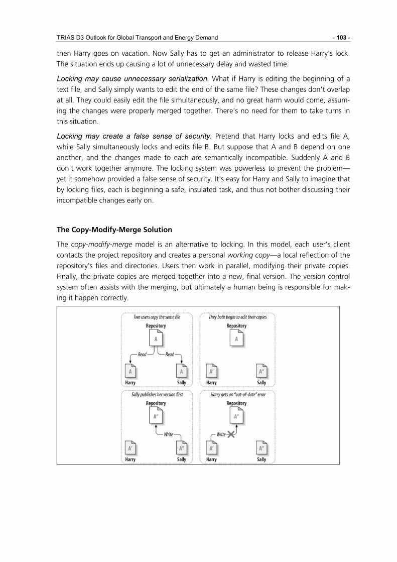
TRIAS D3 Outlook for Global Transport and Energy Demand - 103 -
then Harry goes on vacation. Now Sally has to get an administrator to release Harry's lock.
The situation ends up causing a lot of unnecessary delay and wasted time.
Locking may cause unnecessary serialization. What if Harry is editing the beginning of a
text file, and Sally simply wants to edit the end of the same file? These changes don't overlap
at all. They could easily edit the file simultaneously, and no great harm would come, assum-
ing the changes were properly merged together. There's no need for them to take turns in
this situation.
Locking may create a false sense of security. Pretend that Harry locks and edits file A,
while Sally simultaneously locks and edits file B. But suppose that A and B depend on one
another, and the changes made to each are semantically incompatible. Suddenly A and B
don't work together anymore. The locking system was powerless to prevent the problem—
yet it somehow provided a false sense of security. It's easy for Harry and Sally to imagine that
by locking files, each is beginning a safe, insulated task, and thus not bother discussing their
incompatible changes early on.
The Copy-Modify-Merge Solution
The copy-modify-merge model is an alternative to locking. In this model, each user's client
contacts the project repository and creates a personal working copy—a local reflection of the
repository's files and directories. Users then work in parallel, modifying their private copies.
Finally, the private copies are merged together into a new, final version. The version control
system often assists with the merging, but ultimately a human being is responsible for mak-
ing it happen correctly.

- 104 - Economic, Transport and Environmental Modelling
Figure 46: The Copy, Modify, Merge Solution
Here is an example. Say that Harry and Sally each create working copies of the same project,
copied from the repository. They work concurrently, and make changes to the same file A
within their copies. Sally saves her changes to the repository first. When Harry attempts to
save his changes later, the repository informs him that his file A is out-of-date. In other
words, that file A in the repository has somehow changed since he last copied it. So Harry
asks his client to merge any new changes from the repository into his working copy of file A.
Chances are that Sally's changes don't overlap with his own; so once he has both sets of
changes integrated, he saves his working copy back to the repository. Figure 46 shows this
process.
But what if Sally's changes do overlap with Harry's changes? This situation is called a conflict,
and it's usually not much of a problem. When Harry asks his client to merge the latest reposi-
tory changes into his working copy, his copy of file A is somehow flagged as being in a state
of conflict: he'll be able to see both sets of conflicting changes, and manually choose be-
tween them. Note that software can't automatically resolve conflicts; only humans are capa-
ble of understanding and making the necessary intelligent choices. Once Harry has manually
resolved the overlapping changes—perhaps after a discussion with Sally—he can safely save
the merged file back to the repository.
The copy-modify-merge model may sound a bit chaotic, but in practice, it runs extremely
smoothly. Users can work in parallel, never waiting for one another. When they work on the
same files, it turns out that most of their concurrent changes don't overlap at all; conflicts are
infrequent. And the amount of time it takes to resolve conflicts is far less than the time lost
by a locking system.
In the end, it all comes down to one critical factor: user communication. When users com-
municate poorly, both syntactic and semantic conflicts increase. No system can force users to
communicate perfectly, and no system can detect semantic conflicts. So there's no point in
being lulled into a false promise that a locking system will somehow prevent conflicts; in
practice, locking seems to inhibit productivity more than anything else (which we sometimes

TRIAS D3 Outlook for Global Transport and Energy Demand - 105 -
could see for the past ASTRA development, where we mostly followed the lock-modify-
unlock approach by appointing someone to be the "model master" for a period during
which the others could not really touch the model).
Using Subversion to Control Versions of ASTRA
One state-of-the-art Version controlling system is Subversion (subversion.tigris.org). We de-
cided using this for various reasons:
• Stable and reliable due to a broad user base and a seven year development history as
an open-source project, which started in 2000.
• Available at no cost.
• Used in many productive software development projects. Outstanding positive feed-
back in software developing communities.
This decision was completely justified by the experiences we made during the TRIAS project.
We had no data loss and all features of the software worked as expected.
Workflow for the model developer
We exclusively used the Copy-Modify-Merge approach to version controlling due to the
drawbacks of the Lock-Modify-Unlock approach as described above. Whenever a model de-
veloper needed exclusive access to certain or all files we agreed on timeframes when the
other developers must not modify the model. This worked without problems and is com-
pletely in line with the philosophy of a version control system. It is intended to support dis-
tributed working. It does not free you from the need to communicate.
The following sections are in parts redundant to the preceding chapter. The intention is to
give a more concrete description of what version controlling means to us as developers of the
ASTRA model. It is written as an instruction to the user.
Getting a Working copy
To get a working copy, you check out files of the repository. This means the software simply
creates a private copy of the files on the server for you locally on your computer.
This working copy is an ordinary directory tree on your local system, containing a collection
of files. You can edit these files however you wish, and in the case of our ASTRA model files
they will work at any time just as if there would be no Version Controlling Server. Your work-
ing copy is your own private work area: Subversion will never incorporate other people's
changes, nor make your own changes available to others, until you explicitly tell it to do so.
Changing your Working Copy
You do your changes. You make sure that your local working copy actually remains a valid
Vensim model.
- 106 - Economic, Transport and Environmental Modelling
Writing changes back
After you've made some changes to the files in your working copy and verified that they
work properly, Subversion provides you with commands to “publish” your changes to the
other people working with you on your project (by writing to the repository).
If other people published their own changes since you downloaded files form the server the
last time, Subversion provides you with commands to merge those changes into your work-
ing directory (by reading from the repository) before you write your files into the repository.
This is the critical moment in any teamwork: bringing together the contributions of the dif-
ferent team members. This cannot be done by a computer. If a file that you worked on has
been modified in the meantime by somebody else, Subversion reports a Conflict and pro-
duces a single file merged from the two available versions. But this is only a recommenda-
tion. You then have to look at the file and make sure that it is correct. Maybe you delete
changes of the other person, or changes you did yourself. If both persons worked on differ-
ent sections of the file, there is probably nothing to delete. Then you check that the com-
bined version works properly, e.g. by making a "syntax check" in Vensim. If everything is
fine, you write the file into the repository, you check in and commit your contribution to the
collective work.
Locking
Even though we clearly prefer copy-modify-merge, there are situations in which locking is
necessary. This is the case especially when changing binary files, such as an Excel file or a
graphic file (e.g. jgp). Also when making a lot of changes in the ASTRA model in one step
locking can make sense. Subversion offers the possibility to work according to the lock-
modify-unlock approach by a simple extra command.
Keeping the model intact
Our most important concern is keeping the model semantically and logically correct. No
software can ensure that. It is us who are responsible for that. And the only way we can
achieve that is by good communication. Various people working on different parts of the
model always have to agree on changes before they happen in order to maintain our model
intact in every sense: semantically correct, logically correct and calibrated.
4.1.7 Additional Maintenance Tools for the Model Development
During the progression of the project, some possibilities for automation of repetitive model-
ling tasks by maintenance and support tools were identified. The solutions were implemented
in differing ways, depending on the technical possibilities offered by certain software tools.

TRIAS D3 Outlook for Global Transport and Energy Demand - 107 -
4.1.7.1 Variable renaming
Splitting the ASTRA model into many modules and sub-modules created the need for a new
way to rename variables. Before, Vensim could handle the task because a single variable
could be renamed at one location on one view and was automatically renamed in the whole
model since this was contained in on single Vensim model file. But as the model was split
into more than 30 (sub-) modules, renaming of a variable would mean to check every single
module whether it contains the according variable and then rename every single occurrence.
This problem was solved by an additional Java application. The user only needs to provide a
list of pairs of current and new variable names in an excel file and a list of the modules, in
which the variables should be renamed and the tool takes care of the renaming.
4.1.7.2 Compile Model Variable Lists
We lacked a way of producing a list of all or some of the variables contained in the ASTRA
model. Based on the regular expressions implemented in the text editor WinEdt 5.5 various
macros were developed to compile list of variables according to various criteria. We now dis-
pose of the possibility to compile variables lists containing:
• All variables.
• All variables together with their subscript definition.
• All variables except those contained in the in group.
• All variables contained in the in group.
• All variables except those of the type lookup.
4.1.7.3 Normalizing Model Files
During the continued work with the merged model files, Vensim continuously adds redun-
dant white space and tabulator characters, making the model source code not very conven-
ient for reading. A WinEdt 5.5 macro was developed to remove these superfluous characters.

- 108 - Economic, Transport and Environmental Modelling
4.2 VACLAV
4.2.1 Description of VACLAV
Passenger demand modelling – methodology
For modelling passenger transport demand the VACLAV model will be applied, which is a
network-based Europe-wide forecasting model for passenger traffic (modes: rail, road, air,
coach). The model structure follows the classic four-step approach of trip generation, trip
distribution, modal choice and trip assignment, considering the trip purposes business, pri-
vate and holiday.
The zonal system underlying the passenger transport demand modelling is NUTS 3, which
results in around 1,300 traffic cells. The geographical scope of the model is the whole Euro-
pean continent (including Ireland and UK), as well as Turkey.
The VACLAV passenger transport model has been applied in several major European projects
such as
• the STEMM project on behalf of the European Commission DG VII,
• the Forecast 2020 study on behalf of the European Commission,
• the Study on traffic forecasts on the Helsinki corridors,
• the Corridor study for the transport corridor Paris – Strasbourg – Stuttgart – München
– Wien,
• the ETIS-BASE project on behalf of the European Commission, DG TREN,
• the TEN-STAC project on behalf of the European Commission, DG TREN,
• the TRANS-TOOLS project on behalf of the European Commission, DG TREN,
• the EUN-STAT project on behalf of the European Commission, DG TREN,
• the Feasibility Study on the Rail Baltica railways on behalf of the European Commis-
sion, DG Regio,
• and the TINA Turkey project, on behalf of the European Commission/ EU Delegation
in Turkey.
The transport model’s basic methodology is illustrated in the following sections per modelling
step.
Generation and distribution
For the stage of traffic generation a methodology is applied, which for each population seg-
ment assumes specific probabilities for the generation of trips by trip purposes. The informa-
tion for these assumptions stems from several household surveys.

TRIAS D3 Outlook for Global Transport and Energy Demand - 109 -
For the distribution of these trips to destinations a gravitation approach is applied, after hav-
ing defined for each traffic cell trip purpose-specific determinants for the generation and the
attraction of trips, like area, population by sex and age classes, GDP per capita, Gross Value
Added by economic sectors, employment, motorisation, climate, landscape and ethnical and
cultural descriptors, as well as geographical data. The number of trips between two traffic cells i and j, ijT , is estimated by:
321)exp( 0ββββ CAGT jiij ⋅⋅⋅= , (eq. 5)
where
iG trip generating elements in origin i
jA trip attracting elements in destination j
C impedance between i and j
kβ model parameter
Modal split
After the computation of the generation and spatial distribution of trips the modal split is
calculated. For each origin-destination pair (i, j) the modal split model estimates the probabil-
ity of selecting a modal alternative m out of a set of available modes. Within VACLAV, the
modal choice set comprises four means of transport:
• Passenger car,
• Rail,
• Air and
• Coach.
The mode-choice is performed simultaneously in just one step. In order to allow a more real-
istic modelling of individuals’ modal choice decisions, a logit function enhanced by a Box-Cox
transformation is used. The choice probability for mode m on an O/D relation (i, j) is calcu-
lated by following formula:
P m | ij( ) =exp Um( )
exp U m'( )m'∈C( i, j )∑
, (eq. 6)
where Um = β m 0 + βmk Xmk(λ mk )
k∑
with )(λx = (x λ − 1)
λλ ≠ 0, x > 0
ln x λ = 0, x > 0
⎧ ⎨ ⎪
⎩ ⎪
The explanatory variables Xmk
(λmk ) ’s represent the transport service level between zones i and j
in the following dimensions:
• total travel costs (including access /egress costs) TTC m | ij( )net travel costs (excluding
access/egress costs) NTC m | ij( )

- 110 - Economic, Transport and Environmental Modelling
• total travel time (in-vehicle + out-of-vehicle + access/egress) TTT m | ij( )
• net travel time (excluding access /egress) NTT m | ij( )
• access / egress distance AED m | ij( )
• total frequency / number of daily connections TFR m | ij( )
• total number of transfers TNT m | ij( )
• car ownership rate of originating zone
The assignment procedure
The final step of the four-stage approach is the assignment of the traffic demand by mode to
the corresponding network models. This implies the task of estimating the users’ route choice
within the transportation networks. For this purpose generalised users costs are calculated
(derived from the utility functions in the mode choice model) for every link in the network
and shortest path algorithms are applied.
Speeds on road links (and therefore their contribution to user costs) depend on the traffic
load situation. This relationship is represented by specific speed-flow and cost-flow functions
for each link type. Link types are formally distinguished with respect to technical standards,
like the number of lanes and the terrain type (slope, bends). Beyond a characteristic load
value (“capacity“), the increase of link flows persistently leads to a speed reduction and
hence an increase of user costs, which is called “congestion effect“. In order to take into
account of the congestion effect, the assignment is applied in an iterative way. The overall
traffic demand is split and assigned step by step, such that the link speeds are adjusted ac-
cording to the new traffic loads after each step.
The assignment tool of the VACLAV model performs the assignment of passenger and
freight transport vehicles simultaneously. The road assignment approach enables the consid-
eration and quantification of congestion effects.
The network models used by VACLAV are based on the GISCO and UIC networks, which
were subject to careful updating for the purposes of the TEN-STAC project, as well as the
ETIS-BASE project. Within the EUN-STAT project the network models have been extended to
the neighbouring countries of the EU, in the TINA Turkey project to Turkey.
The following maps illustrate the network models for rail and road for the year 2003.
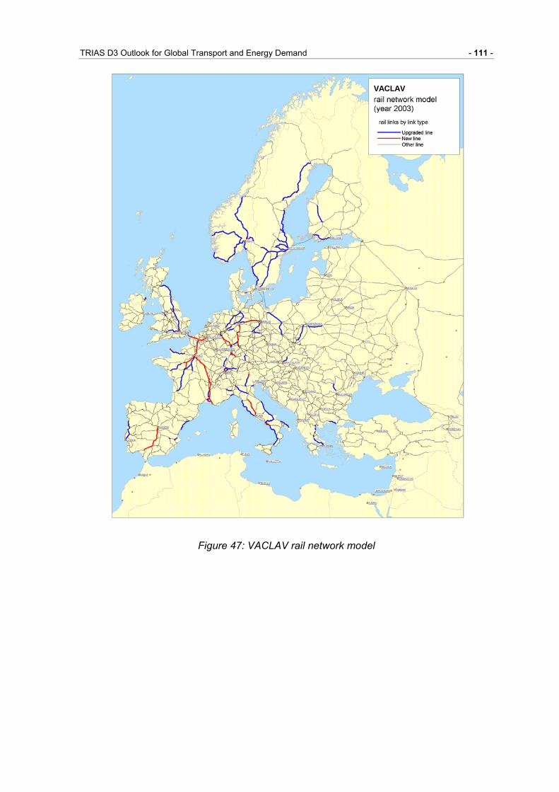
TRIAS D3 Outlook for Global Transport and Energy Demand - 111 -
Figure 47: VACLAV rail network model

- 112 - Economic, Transport and Environmental Modelling
Figure 48: VACLAV road network model
4.2.2 Extension to 2030
For the extension of VACLAV to 2030 three inputs needed to be prepared:
• The policies and costs had to be defined,
• rail and road networks had to be adapted to 2030 and
• demand matrices for passengers and freight for 2030 had to be computed.
For the policies and costs, input was taken from ASTRA and harmonized to the current inputs
of the years 2000-2020.

TRIAS D3 Outlook for Global Transport and Energy Demand - 113 -
The networks have been adapted to provide scenario information for the years 2010 and
2030. For 2030 all TEN projects are included. To create demand matrices for 2010, 2020 and
2030 growth rates for passenger and freight trips were taken from ASTRA and applied to the
VACLAV base year matrix. For further information see next chapter Linkage to ASTRA.
Figure 49: VACLAV rail network for 2030

- 114 - Economic, Transport and Environmental Modelling
Figure 50: VACLAV road network for 2030

TRIAS D3 Outlook for Global Transport and Energy Demand - 115 -
4.2.3 Linkage to ASTRA
The linkage between VACLAV and the ASTRA model has been established with the aim of
improving the modelling of the interaction between road demand and supply and of the im-
pact of additional transport infrastructures on travel times. Being a transport network model,
VACLAV can provide detailed results about travel time and its sensitiveness to the changes of
the demand/supply ratio is obviously higher than ASTRA. At the same time, ASTRA and
VACLAV are two separate and independent models, therefore the linkage between the two
has been conceived such as the interaction is not necessarily required to run the ASTRA
model. In brief, the linkage between ASTRA and VACLAV can work in two different ways:
• “tight linkage”: the two models run together, exchanging variables automatically;
• “loose linkage”: ASTRA runs using exogenous inputs from VACLAV.
The difference between the two kind of linkage is in the automation of the data exchanging,
but also in the bi- directional exchange which takes place in the “tight” linkage compared to
the mono-directional exchange (from VACLAV to ASTRA) which occurs in the “loose” link-
age.
In the “tight” linkage, the results of the assignment phase in VACLAV is firstly aggregated
according to the ASTRA zoning system (i.e. by country and distance band). As VACLAV deals
with “inter-urban” trips and local mobility is not really simulated, only results for the re-
gional, medium and long distance bands within ASTRA are produced. The following main
variables are built on VACLAV assignment results:
• Average speed (time per km) on long distance road network (by origin/destination
pair and distance band);
• Share of demand using tolled motorways (by origin/destination pair and distance
band).
The average speed is used in ASTRA to compute the generalised cost of road trips for each
O/D pair. While the share of demand using tolled motorways is used in ASTRA to compute
the weighted average cost of road trips for each O/D.
VACLAV runs for four time thresholds (years 2000, 2010, 2020 and 2030), for the intermedi-
ate years (as ASTRA needs data per each year) is obtained by interpolating such four values.
The ASTRA model reads these variables by means of suitable functions programmed as ex-
ternal libraries and included in the ASTRA structure. The ASTRA base speed by O/D is there-
fore updated using the trend read from the VACLAV results and the model uses the updated
speed trend and the share of demand using tolled motorways in order to compute the modal
split over the simulation period.
Then, the trip matrix by mode for the years 2000, 2010, 2020 and 2030 is extracted from
ASTRA and split up into the detailed VACLAV zoning system using pre-defined exogenous
shares. Such new matrices are used again in VACLAV for a new assignment. The whole pro-
cedure iterates until the results of the VACLAV assignment reach an equilibrium.

- 116 - Economic, Transport and Environmental Modelling
In the “loose” linkage the procedure is simpler as there just a transfer of information from
VACLAV to ASTRA. The same two variables as above (average speed and share of demand
using tolled motorways) are extracted from VACLAV plus a third variable: the share of con-
gested long distance road network (by country). This third variable is used in the ASTRA to
compute the average speed using the aggregate speed-flow function. VACLAV produces and
provides the input variables only once, afterwards ASTRA is run autonomously.
The software PVM (parallel virtual machine) has been incorporated into the ASTRA external
function library and VACLAV to enable the direct communication between Windows com-
puter based ASTRA and Linux computer based VACLAV. This allows functions in the external
library to start VACLAV on the Linux cluster and to directly exchange data between those
two platforms.
The creation of the demand matrices for VACLAV posed more problems than expected. The
disaggregation of the matrices for the VACLAV base year 2000 yielded some structural dif-
ferences, which could not be resolved. The second approach, were demand growth rates
from ASTRA were applied directly on the base year matrices in VACLAV, resulted in better
results, but still there were regional problems which could not be matched to former assign-
ments. Also these two approaches disabled the modal split in VACLAV since the modal split
from ASTRA between functional zones was used. A third setup in which only demand
growth rates before the modal split were transferred revealed the same regional problems.
IWW is currently working on a methodology to overcome these problems. In order to pre-
serve the structure of the current VACLAV demand matrices new matrices are computed
from the ASTRA demand matrices using weight information from VACLAV and a furness
iteration algorithm to balance the matrices.
4.3 Regio-SUSTAIN
4.3.1 Description of Regio-SUSTAIN
Regio-SUSTAIN has been developed at the Institute of Economic Policy Research (IWW). It is
used as a model to assess the impacts of traffic-related emissions on human beings. Com-
parisons between different policies and transport scenarios can be estimated with Regio-
SUSTAIN. The outcome of the model is two-fold: On the one hand side the local immissions
and on the other side the number of inhabitants affected by a special substance, such as NOx,
PM or noise, can be computed.
The core of the model is a comprehensive database, programmed in PostgreSQL (an open-
source SQL-database especially for use with spatial data). Inputs to the database are either
available from open sources or are computed with external software belonging to IWW.
General inputs are spatial data about land cover (in grids of 250m), population numbers and
climate/weather conditions from national or international geographical information systems.
Beside the general inputs, network related data are necessary, such as network links and traf-
fic numbers.
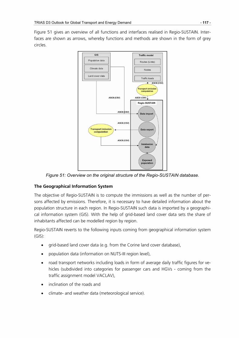
TRIAS D3 Outlook for Global Transport and Energy Demand - 117 -
Figure 51 gives an overview of all functions and interfaces realised in Regio-SUSTAIN. Inter-
faces are shown as arrows, whereby functions and methods are shown in the form of grey
circles.
Figure 51: Overview on the original structure of the Regio-SUSTAIN database.
The Geographical Information System
The objective of Regio-SUSTAIN is to compute the immissions as well as the number of per-
sons affected by emissions. Therefore, it is necessary to have detailed information about the
population structure in each region. In Regio-SUSTAIN such data is imported by a geographi-
cal information system (GIS). With the help of grid-based land cover data sets the share of
inhabitants affected can be modelled region by region.
Regio-SUSTAIN reverts to the following inputs coming from geographical information system
(GIS):
• grid-based land cover data (e.g. from the Corine land cover database),
• population data (information on NUTS-III region level),
• road transport networks including loads in form of average daily traffic figures for ve-
hicles (subdivided into categories for passenger cars and HGVs - coming from the
traffic assignment model VACLAV),
• inclination of the roads and
• climate- and weather data (meteorological service).

- 118 - Economic, Transport and Environmental Modelling
The Central Database Function – Population Density
Land cover data comes from the European Corine database, which provides consistent in-
formation on land cover and land cover changes across Europe over the past decades. Regio-
SUSTAIN uses 250 x 250m grids as reference for calculation.
The Corine land cover database defines two urban classes, namely “Urban dense” and “Ur-
ban discontinuous” for Europe. Further 42 land use categories are defined which are not
related to human habitation. According to a publication by Gallego (2001), only about
82.5% of the total population in Germany can be assigned to the two urban land cover
types. The remaining 17.5% of the population has to be assigned to the other land cover
categories (5,392,062 elements). Based on statistical analyses, Gallego presented distribution
values for several European countries, for each type of Corine land cover. These distribution
values are adopted for the allocation of the population for all land cover types in Regio-
SUSTAIN. This might need some clarification:
As an example, the population distribution function of Gallego assigns 28.9% of cells to the
CLC class “pasture” in Ireland. This does not mean that 28.9% of the Irish population live in
pasture fields, but that 28.9% of the population live in cells, which are defined as “pasture”.
This may correspond to a large number of small urban villages within the CLC “pasture”
class.
Figure 52 shows an example of CLC data sets in a specific area. It describes an example for
calculating the population density for CLC categories. The sample area consists of 9 cells (250
x 250m) and covers an area of 0.56 km² (from the CLC database the following information
are available: 78% forest, approx. 11% urban dense and approx. 11% Urban discontinuous).
It includes a small village with about 100 inhabitants (information based on the Seamless
Administrative Boundaries of Europe (SABE) - database). Furthermore, it is known that 30%
of the inhabitants live in the category “Urban dense”, 70% in “Urban discontinuous” and
nobody in “Forest”.
Based on these values average population numbers for every CLC category can be estimated.
30 persons are allocated to “Urban dense”, 10 to “Urban discontinuous” and nobody to
“Forest”. Information about the population per region/ polygon (from SABE) is blended with
the associated CLC data, which is covered by this polygon.
The approach described by Gallego has been modified by Schmedding (2005). The improve-
ment has been necessary when analysing smaller regions instead of countries like Gallego
did. The improved methodology uses the country shares per CLC category of Gallego and
multiplies the results with a correction factor. The factor depends on the number of cells be-
longing to each CLC category and the number of persons allocated to each region by the
approach of Gallego. In the case that one CLC category does not exist in an area under con-
sideration, the number of fictitious allocated persons by Gallego have to be reallocated to the
existing categories.
The reallocated number of persons has been inserted in the Regio-SUSTAIN database and is
used in the TRIAS project.

TRIAS D3 Outlook for Global Transport and Energy Demand - 119 -
Figure 52: Example of land cover data
Calculation of Emission Levels
At the Institute for Economic Policy Research different Java based models have been devel-
oped to calculate transport emissions per kilometre in the area under consideration. Average
emissions are calculated for each link of the network and are depending on the road struc-
ture in the network, the number of vehicles on the roads, the vehicle fleet on the link and the
regional elevation profile. Average emission factors for each vehicle category are taken from
the Handbook of Emission Factors published by Infras AG for the German and Swiss Envi-
ronmental Agency. The output of the Java models is average emission values per km of each
network link that are stored in the database and is used for immssion calculations.
Calculation of Immission Levels
Immission levels are modelled with an external software, called SoundPlan, which has been
developed by Braunstein & Berndt GmbH in Backnang (Germany). SoundPlan is a compre-
hensive software package offering noise and air pollution evaluation modules. Using the in-
puts of Regio-SUSTAIN (emission concentration, road transport network including loads)
SoundPlan calculates immission for pre-defined grids (e.g. 250x250m).
Number of affected people
In the last step the information about population density and immission values per grid are
merged to calculate the number of affected people. Therefore, concrete exposure levels as
well as very precise categories can be defined to get a detailed picture about the environ-
mental impacts of the transport network. The number of exposed people to NOx, to soot
particles and to other emission substances can be compared to international environmental
quality standards, which are defined for example by the German Environmental Agency in
1997. The database analyses each grid of the region under consideration and calculates the
population number of that specific grid. Aggregating the information about immission values
and population numbers lead to the final output of Regio-SUSTAIN the number of affected
people by a specific concentration of a given substance, such as NOx, PM or noise.

- 120 - Economic, Transport and Environmental Modelling
4.3.2 Extension to Point Emissions (POLES)
Industrial emissions into air and water from facilities in EU-15 countries for the year 2001
have been registered in the European Pollutant Emission Register (EPER) database of the
European Commission. With growth rate calculated from the Prospective Outlook on Long
Term Energy System (POLES) energy model and information on emission factor and abate-
ment technology obtained from the RAINS-GAINS database of International Institute for Ap-
plied Systems Analysis, some of the emissions (NOx and PM10) have been projected to the
2050 horizon.
4.3.2.1 European Pollutant Emission Register (EPER)
In the article 15 of the Integrated Pollution Prevention and Control (IPPC) Directive, the main
purpose of a European Commission emission inventory will be to collect and store compara-
ble emission (to air and water) data of individual polluting industrial sources and activities
into an integrated database or register and to provide public accessibility to the registered
data. Only emission to air and water are considered as emissions. The data of the current of
the existing register, being named as European Pollutant Emission Register (EPER) whose de-
cision was published in the Official Journal of the European Communities under reference
2000/479/EC (17 July 2000), is delivered to the Commission by the national governments of
the Member States and this will be updated periodically.
According to the Guidance Document for EPER Implementation1, the EPER will be used as a
public register to provide environmental information on industrial activities covered by the
IPPC Directive2 and has the following objectives related to different groups of users:
to enhance awareness for environmental pollution and to compare emissions by individual
facilities or industrial sectors. Making the data accessible on an Internet site will increase the
public use of the EPER data by non-governmental organisations and research organisations or
interested citizens (public use);
to trigger industry in improving environmental performance and innovating industrial proc-
esses. The achievements by industry will result into emission reductions that can be moni-
tored and demonstrated in the EPER register (industry use);
to evaluate the progress of achievements in meeting environmental targets in national or
international agreements; the EPER enables the Commission to identify principal emissions
and industrial sources, assess the reported data of Member States with respect to some in-
ternational agreements and to publish the results periodically (government use).
The data submission regulated by OJ 2000/479/EC or known as "EPER Decision"3 should be
conducted by Member States including all individual facilities with one or more activities as
mentioned in Appendix I to Council Directive 96/61/EC or known as the IPPC Directive. The
1 http://www.eper.cec.eu.int/eper/documents/eper_en.pdf 2 http://eur-lex.europa.eu/LexUriServ/LexUriServ.do?uri=CELEX:31996L0061:EN:HTML 3 http://eper.cec.eu.int/eper/documents/comission_17072000.pdf

TRIAS D3 Outlook for Global Transport and Energy Demand - 121 -
Commission Decision (EPER Decision) gives details of the list of pollutants to be reported (and
its threshold value), the report format, emission source categories and their corresponding
(NOSE-P) codes to be reported, and the definition used in EPER.
The mandatory reporting of emissions according to the requirements of the EPER Decision is
a stepwise process with the following key elements (Guidance Document for EPER Implemen-
tation):
Identifying and selecting the facilities with Appendix I activities. Article 1, sub 1 of the EPER
Decision requires Member States to report emissions from all individual facilities with one or
more activities as mentioned in Appendix I of the IPPC Directive. These activities are identified
by the source categories as specified in Appendix A3 of the EPER Decision.
Determining pollutant specific emissions from all individual facilities with Appendix I activities.
Article 1, sub 2 of the EPER Decision requires Member States to include in the report the
emissions to air and water for all pollutants for which the threshold values are exceeded.
Both pollutants and threshold values are specified in Appendix A1 of the EPER Decision.
Reporting the emissions for individual facilities with Appendix I activities. The emission data
shall be reported for each facility according to the format of Appendix A2 of the EPER Deci-
sion (Article 1, sub 3). Member States are required to provide this report on CD-ROMs.
Reporting aggregated emission data for all pollutants of Appendix A3 of the EPER Decision in
an overview report. This overview report includes the national totals of all individually re-
ported emissions for both each of the source categories and the NOSE-P codes as specified in
Appendix A3 of the EPER Decision (Article 1, sub 4). Member States shall provide this over-
view report on paper and on CD-ROMs.
Disseminating all reported data by the Commission. The Commission will make the facility
specific data as well as the aggregated data provided by each Member State publicly accessi-
ble on the Internet (Article 4).
The current EPER database4 contains emissions information of industrial facilities of EU-15
countries for the year of 2001. The member countries submitted this report data on June
2003. The second reporting year was on June 2006, which should include report of the year
2004. After review and evaluation in 2006 a decision can be taken on a subsequent annual
reporting by Member States in December of the year T on releases in the year T-1. From
2008 onwards, the Member States are encouraged to have a regular reporting system in
place and send annual report to the Commission in December of year T, instead of June a
year later (T+1). As many international protocols require emission reporting in December, a
future reporting in December will be enable Member States to synchronise the EPER report-
ing with other international reporting requirements (UNFCC, UN/ECE, etc.)
4 http://www.eper.cec.eu.int/eper/

- 122 - Economic, Transport and Environmental Modelling
4.3.2.2 Regional Air Pollution Information and Simulation (RAINS) and the Green-house Gas and Air Pollution Interactions and Synergies (GAINS)
The Regional Air Pollution Information and Simulation (RAINS) model developed by the Inter-
national Institute for Applied Systems Analysis (IIASA) combines information on economic
and energy development, emission control potentials and costs, atmospheric dispersion char-
acteristics and environmental sensitivities towards air pollution (Schöpp et al., 1999). The
model addresses threats to human health posed by fine particulates and ground-level ozone
as well as risk of ecosystems damage from acidification, excess nitrogen deposition (eutrophi-
cation) and exposure to elevated ambient levels of ozone.
These air pollution related problems are considered in a multi-pollutant context (Figure 53),
quantifying the contributions of sulphur dioxide (SO2), nitrogen oxides (NOx), ammonia
(NH3), non-methane volatile organic compounds (VOC), and primary emissions of fine
(PM2.5) and coarse (PM10-PM2.5) particles (Table 33). The RAINS model also includes esti-
mates of emissions of relevant greenhouse gases such as carbon dioxide (CO2) and nitrous
oxide (N2O). Current work is progressing to include methane (CH4) as another direct green-
house gas as well as carbon monoxide (CO) and black carbon (BC) into the model frame-
work.
Table 33: Multi-pollutant/multi-effect approach of the RAINS model
Primary PM SO2 NOx VOC NH3
Health im-pacts:
- PM
- O3
Vegetation impacts:
- O3
- Acidification
- Eutrophicati-on
Source: Amann et al., 2004

TRIAS D3 Outlook for Global Transport and Energy Demand - 123 -
Figure 53: Flow of information in the RAINS model
Source: Amann et al., 2004
The European implementation of the RAINS model incorporates databases on energy con-
sumption for 40 regions in Europe, distinguishing 22 categories of fuel use in six economic
sectors. The time horizon extends from the year 1990 up to the year 2030. Emissions of SO2,
NOx, NH3, and VOC for 1990 are estimated based on information collected by the CORINAIR
905 inventory of the European Environmental Agency and on national information. Options
and costs for controlling emissions of the various substances are represented in the model by
considering the characteristic technical and economic features of the most important emis-
sion reduction options and technologies. A detailed description of the RAINS model, on-line
access to certain model parts as well as all input data to the model can be found on the
Internet6.
The RAINS model has two capabilities:
scenario analysis: in which the model is able to estimate the (economic) costs and environ-
mental effects of an exogenously assumed pattern of emission controls;
optimisation mode: in which the model using a non-linear optimisation mode is capable to
identify the least-cost allocation of emission controls that meet exogenously determined envi-
ronmental targets. This enables the development of multi-pollutant, multi-effect pollution
5 http://reports.eea.europa.eu/92-9167-022-7/en/ 6 http://www.iiasa.ac.at/rains
- 124 - Economic, Transport and Environmental Modelling
control strategies. In particular, the optimisation can be used to search for cost-minimal bal-
ances of controls of the six pollutants (SO2, NOx, VOC, NH3, primary PM2.5, primary PM10-
2.5(=PM coarse)) over the various economic sectors in all European countries that simultane-
ously achieve user-specified targets for human health impacts, ecosystem protection, and
maximum allowed violations of WHO guideline values for ground-level ozone, etc.
Over the last years, IIASA has extended its RAINS model to explore synergies and trade-offs
between the control of local and regional air pollution and the mitigation of global green-
house gas emissions. This new GAINS (Greenhouse Gas and Air Pollution Interactions and
Synergies) model assists in the search for pollution control strategies that maximise benefits
across all scales.
The European implementation of the GAINS model has been released in December 2006. It
covers 43 countries in Europe. This new GAINS model incorporates the latest version of the
RAINS-Europe as it has been prepared for the 2007 of the National Emission Cellings Direc-
tive7 resulted from bilateral consultations between IIASA modelling team and national ex-
perts of the IIASA country members. GAINS combines it with estimates of emissions, mitiga-
tion potentials and costs for the six greenhouse gases included in the Kyoto protocol, fully
compatible with the methodology applied for the conventional air pollutants. GAINS-Europe
is implemented on the Internet and an online version8 is available.
4.3.2.3 Methodology
Results and information from the two models, RAINS-GAINS and POLES, and EPER database
are combined to produce the projection of CO2, NOx, and PM10.
Information from EPER Database
EPER database provides information on industrial facilities in each of EU-15 countries for the
year 2001. In the data structure, as seen in Figure 54, the emission information is detailed in
type, value, method, pollutant name, and facility name. The emission types are water and/or
air, the value is expressed in ton of pollutant, the method are described measured and/or
calculated, and the pollutant name follows the pollutant identification as given by the ap-pendix A1 of the EPER decision.
7 http://www.iiasa.ac.at/rains/nec2007.html?sb=18 8 http://www.iiasa.ac.at/rains/gains-online.html

TRIAS D3 Outlook for Global Transport and Energy Demand - 125 -
Figure 54: EPER Data Structure
Results and Projection from POLES Reference Scenario
POLES energy model is able to give projection on world long-term energy projections, na-
tional-regional energy balance and CO2 emission simulation, analysis of new energy technol-
ogy potentials, markets and diffusion, and test of energy policies and energy RTD strategies.
The actual POLES energy model has the capacity to produce those outputs until 2050 hori-
zon. In order to project NOx and PM10 emissions to the 2030 horizon, a Business as Usual or
Reference scenario has been run and result for fuel consumption per country (of the EU-15)
and per sector have been extracted.
The POLES Reference scenario describes the economic and technological fundamentals that
determine the dynamics of the world energy system; it also includes elements of policy or
political development that are likely to occur in the period. It reflects the geo-political con-

- 126 - Economic, Transport and Environmental Modelling
juncture that dominates the short and medium-term availability and price of world oil; it also
reflects a minimum degree of political initiative in climate policy in all regions of the world.
The Reference case accordingly visualizes a world adjusting to constraints on access to oil and
gas and on emissions of CO2.
The Reference case represents the "minimum" climate policies by an exogenous carbon value
that modifies the investment and consumption decisions of the economic agents. It assumes
that Europe keeps the lead in climate policies, although in this case these policies are devel-
oped in a minor key. Assumption used for carbon value in Europe is in line to the estimates
provided by the European Emission Trading System9. The POLES' Reference scenario has been
used as a reference scenario in World Energy and Technology Outlook 2050 (WETO-H2 Pro-
ject)10 of the DG-Research Commission European under the 6th Framework Programme.
Information and Results from RAINS Model Database
The central objective of the integrated assessment models it to assist in the cost-effective
allocation of emission reduction measures across various pollutants, several countries and
different economic sectors. In order to capture these differences across Europe in a system-
atic way, a methodology has been developed to estimate the emissions and emission control
costs of standard technologies under the specific conditions characteristic for the various
European countries11.
The methodology of emissions estimation consists in aggregation schemes for the emission
sources, energy scenarios development, options for emissions reduction, cost evaluation, and
control strategies and cost curves. The section of aggregation schemes for the emission sources is particularly relevant for the work conducted.
For the NOx, the RAINS model groups first the emission generating activities into sectors of
economic activities which can be called as the Primary RAINS sectors (centralized power plants and district heating, fuel conversion other than power plants, domestic, commercial,
and agricultural use, transportation, industrial, non-energy use-feedstocks and other emission
source). In order to take into account more factors which are highly relevant for emission
generation, the primary sectors are divided into secondary sectors. For example power plants
and district heating as primary sector is divided into new boilers, existing boilers – dry bot-
tom, existing boiler- wet bottom. Those economic sector groups are further subdivided into
9 Kyoto Protocol Implementation study for DG Environment with the POLES model:
http://europa.eu.int/comm/environment/climat/pdf/kyotoprotocolimplementation.pdf 10 http://ec.europa.eu/research/fp6/ssp/weto_h2_en.htm 11 RAINS internet side provides documentations of methodologies used to calculate emissions in
the framework of an integrated assessment model for the analyses carried out for the NEC di-rective in 1998/99. The actual data for 2004 review are available from the on-line version of the RAINS model. However the documentations of methodologies from 1998/99 are very rele-vant to understand the principles of emissions calculations.
TRIAS D3 Outlook for Global Transport and Energy Demand - 127 -
the type of fuel. Complete information in this aggregation could be seen at Cofala and Syri
(1998)12.
For the PMx, the aggregation objective is to categorise the emission producing processes into
a reasonable number of groups with similar technical and economic properties. One impor-
tant requirement in aggregating emission sources is that it should include only source catego-
ries with a contribution of at least 0.5 percent to the total anthropogenic emissions in a par-
ticular country.
The emission sources are divided first into nine primary sectors: stationary combustion, proc-
ess emissions, mining, storage and handling, road transport, off-road transport, open burn-
ing of waste, agriculture, and other source. These nine primary sectors are categorised into
three big primary sector groups: stationary combustion sources, stationary non-combustion
sources, and mobile sources, which are in turn split by relevant fuel types. Some groups are
further disaggregated to distinguish, for example, between existing and new installation in
power plants, or between tire and brake wear for non-exhaust emission from transport. Full
list of RAINS PMx sectors could be seen in Klimont, et al. (2002)13.
Finally for all pollutants, RAINS the emission estimating is conducted in country level. The
calculations are performed for 36 European countries and four sea regions within the EMEP
modelling domain. In addition, Rusia (because of the large geographical area) and Germany
(because of the implementation differences in the base year 1990) are further divided into
sub-national regions.
4.3.2.4 Compatibility
EPER and POLES Sectors Compatibility
In the EPER database, each industrial facility corresponds to one economic activity category as
described by the NACE code14. There are 344 economic sectors identified by NACE Code in
EPER database and they belong into 4 big sections:
• Section C: mining and quarying (21 activities)
• Section D: manufacturing (318 activities, grouped into 12 subsections)
• Section E: electricity, gas, and water supply (4 activities)
• Section O: other community, social and personal service activities (1 activity: sewage
and refuse disposal, sanitation and similar activities)
On the other side, four energy source sectors are identified in POLES: steel industries (STI),
chemical industry (CHI), non metallic mineral industry (NMM), service (SER), and other indus-
12 http://www.iiasa.ac.at/%7Erains/reports/noxpap.pdf 13 http://www.iiasa.ac.at/rains/reports/ir-02-076.pdf 14 The NACE nomenclature (National Classification of Economic Activities) is the European classi-
fication of economic activities. It is based on economic sectors and is composed of four digits (there is a fifth one for national use). The first two digit codes indicate the divisions, the third-digit codes indicate the groups, the fourth-digit codes indicate the classes.

- 128 - Economic, Transport and Environmental Modelling
tries (OIN). POLES model exclude the four activities in the section E of EPER (electricity, gas,
and water supply), so finally, the rest 340 economic sectors identified within industrial facili-
ties registered in EPER database enter one of the 5 energy source sectors in POLES (see ap-pendix 1). Most of the activities are categorised in OIN sectors (238 activities), followed by
STI (47), NMM (31), CHI (24) and SER (1).
POLES and RAINS-GAINS Fuels and Sectors Compatibility
As explained previously, emissions data and result in RAINS-GAINS are categorised into sec-
tors (and sub-sectors) of activities and fuel types in the country level. In POLES model, the
data and results are as well categorised into sector (as mention in Table 35 and in the previ-
ous section) and fuel in the country level. However these aggregations are not directly com-
patible.
For fuel type, POLES energy model is simply differentiated in gas, oil, and coal fuel. In RAINS-
GAINS, the fuel type division is more detailed. The coal, for example, is divided into eight
type of coal and several types of fuel in RAINS-GAINS are not represented in POLES energy
model. The coal fuel from POLES has to be divided into 8 (eight) coal types available in
RAINS-GAINS. This "fuel split" of POLES' coal is made possible by the existing information on
coal percentage in RAINS-GAINS. The relationship between POLES and RAINS-GAINS fuel
type is presented in Table 34 below.

TRIAS D3 Outlook for Global Transport and Energy Demand - 129 -
Table 34: POLES – RAINS-GAINS fuel type relationship
RAINS-GAINS fuels POLES fuels Brown coal/lignite, grade 1 (BC1)
Brown coal/lignite, grade 2 (BC2)
Hard coal, grade 1 (HC1)
Hard coal, grade 2 (HC2)
Hard coal, grade 3 (HC3)
Derived coal (DC)
Other solid-low S (OS1)
Other solid-high S (OS2)
COAL
Heavy fuel oil (HF) n/a
Medium distillates (MD) OIL
Light fractions (LF) n/a
Natural Gas (incl. other gas) GAS
Renewable (solar, wind, small hydro) n/a
Hydro n/a
Nuclear n/a
Electricity n/a
Heat n/a
No fuel use n/a
For NOx from stationary sources, the sector desegregation in RAINS is more detailed than
that in POLES (Table 35 below).
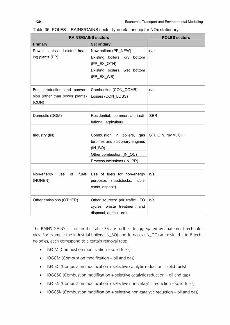
- 130 - Economic, Transport and Environmental Modelling
Table 35: POLES – RAINS/GAINS sector type relationship for NOx stationary
RAINS/GAINS sectors Primary Secondary
POLES sectors
New boilers (PP_NEW)
Existing boilers, dry bottom (PP_EX_OTH)
Power plants and district heat-ing plants (PP)
Existing boilers, wet bottom (PP_EX_WB)
n/a
Combustion (CON_COMB) Fuel production and conver-sion (other than power plants) (CON)
Losses (CON_LOSS)
n/a
Domestic (DOM) Residential, commercial, insti-tutional, agriculture
SER
Combustion in boilers, gas turbines and stationary engines (IN_BO)
Other combustion (IN_OC)
Industry (IN)
Process emissions (IN_PR)
STI, OIN, NMM, CHI
Non-energy use of fuels (NONEN)
Use of fuels for non-energy purposes (feedstocks, lubri-cants, asphalt)
n/a
Other emissions (OTHER) Other sources: (air traffic LTO cycles, waste treatment and disposal, agriculture)
n/a
The RAINS-GAINS sectors in the Table 35 are further disaggregated by abatement technolo-
gies. For example the industrial boilers (IN_BO) and furnaces (IN_OC) are divided into 6 tech-
nologies, each correspond to a certain removal rate:
• ISFCM (Combustion modification – solid fuels)
• IOGCM (Combustion modification – oil and gas)
• ISFCSC (Combustion modification + selective catalytic reduction – solid fuels)
• IOGCSC (Combustion modification + selective catalytic reduction – oil and gas)
• ISFCSN (Combustion modification + selective non-catalytic reduction – solid fuels)
• IOGCSN (Combustion modification + selective non-catalytic reduction – oil and gas)

TRIAS D3 Outlook for Global Transport and Energy Demand - 131 -
Unfortunately, the information on abatement technology split for each sector is so far un-
available. For practical reason, the arithmetical average of removal rate from the existing
technologies is then calculated to obtain the removal rate of abatement technology for the
corresponding sector.
For the PM10, similar to NOx, the STI, OIN, NMM, and CHI sectors from POLES enter into
industry (IN) primary sector of RAINS-GAINS while SER corresponds to domestic (DOM) pri-
mary sector of RAINS-GAINS. However, RAINS-GAINS information or results are disaggre-
gated into secondary sector or sub-sector which means that POLES information or results
have to be disaggregated into the same level of sub-sector. For example: in RAINS-GAINS,
the domestic sector (DOM) in stationary sources is divided into 7 (seven) following sub-
sectors:
• combustion of liquid fuels (DOM)
• fireplaces (DOM_FPLACE)
• stoves (DOM_STOVE)
• single house boilers (<50 kW) – manual (DOM_SHB_M)
• single house boilers (<50 kW) – automatic (DOM_SHB_A)
• medium boilers (<1 MW) – manual (DOM_MB_M)
• medium boilers (<50 MW) – automatic (DOM_MB_A)
A combination of sector and fuel from POLES, for example SER-coal (BC1) which corresponds
to DOM-BC1 in RAINS-GAINS, has to be split then into seven sub-sectors. This is possible
since the information on each sub-sector use percentage is available. However, in this work,
no sub-sector split is conducted. For the sake of simplicity, the sub-sector with the highest
percentage is chosen instead of a sub-sector split. In this example, the DOM_MB_A-BC1 is
chosen since the DOM_MB_A sub-sector has the highest use percentage for the DOM_BC1
combination.

- 132 - Economic, Transport and Environmental Modelling
Table 36 shows the relationship between POLES' sector-fuel and RAINS-GAINS' sector-fuel
for the stationary PM10 emission.
Table 36: POLES – RAINS/GAINS sectors and fuel types relationship for PM10 stationary
POLES Sectors POLES fuels RAINS sectors and fuels (Emission from fuel combustion)
OIL IN_OC_MD
GAS IN_OC_natural gas
IN_OC3-BC1
IN_OC3-BC2
IN_OC3-HC1
IN_OC3-HC2
IN_OC3-HC3
IN_OC-DC
IN_OC-OS1
STI, OIN, CHI, NMM
COAL
IN_OC-OS2
OIL DOM_MD
GAS DOM
DOM_MB_A-BC1
DOM_MB_A-BC2
DOM_MB_A-HC1
DOM_MB_A-HC2
DOM_MB_A-HC3
DOM_STOVE-DC
DOM_STOVE-OS1
SER
COAL
DOM_STOVE-OS2
Furthermore, the same as in the NOx, the sub-sector in PM10 emission above is disaggre-
gated into abatement technology which corresponds to the removal rate or efficiency. In the
power plants and industry, some of those technologies are:
• cyclone (CYC),
• wet scrubber (WSCRB),
• electrostatic precipitator 1 field (ESP1), 2 fields (ESP2) and 3 fields and more (ESP3),
• wet electrostatic precipitator (WESP),
• fabric filters (FF),
• regular maintenance, oil fired boiler (GHIND),
• regular maintenance, domestic oil boiler (GHDOM).
TRIAS D3 Outlook for Global Transport and Energy Demand - 133 -
4.3.2.5 Projection Method
The abated PM10 emission is obtained simply by summing up, for all fuel types, the multipli-
cation of emission factor, fuel consumption, and the abatement rate. The emission factor, as
a constant coefficient, is obtained from RAINS/GAINS while the fuel consumption is produced
by POLES.
∑ −=f
fififjifjiji ypryreyfcefyP ))(*)((1(*)(*)( ,,,,,,, (1) (eq. 7)
P: PM10 emissions in country i, year y, and sector j ef: emission factor of fuel f, from sector j, in country i
fc: fuel consumption of fuel f, from sector j, in country i
re: removal efficiency in country i for fuel f pr: penetration rate of abatement technology in country i for fuel f
RAINS/GAINS provides the removal efficiency rate and the penetration rate of the abatement
technologies for the years 1990, 1995, 2000, 2005, 2010, 2015, 2020, 2025, and 2030. The
between years values are calculated by assuming a linear growth.
The growth rate of this emission per country and per sector is then applied as multiplier to
the EPER database PM10 emission of the year 2001 for each industrial facility to obtain the
PM10 emission projection of each facility for the period of 2001 to 2030.
The growth rate of the PM10 emission of each installation is assumed to be equal to the
growth rate of the PM10 emission of the corresponding country and sector and the installa-
tion production technology related to the PM10 emissions is assumed to remain unchanged
during the observed period.
The abated NOx emission is as well obtained by summing up, for all fuel types, the multiplica-
tion of emission factor and fuel consumption taken into account the removal efficiency and
penetration rate of the abatement technology (eq. 2 below). The emission factor (constant),
the removal and penetration rate (for the same years as PM10) are obtained from
RAINS/GAINS while the fuel consumption from POLES.
∑ −=f
fififjifjiji ypryreyfcefyN ))(*)((1(*)(*)( ,,,,,,, (2) (eq. 8)
N: NOx emissions in country i, year y, and sector j
ef: emission factor of fuel f, from sector j, in country i fc: fuel consumption of fuel f, from sector j, in country i
re: removal efficiency in country i for fuel f
pr: penetration rate of abatement technology in country i for fuel f
The growth rate of abated NOx emission of each installation is assumed to be equal to the
growth rate of the abated NOx emission of the corresponding country and sector and the

- 134 - Economic, Transport and Environmental Modelling
installation production technology related to the abated NOx emissions is assumed to remain
unchanged during the observed period.

TRIAS D3 Outlook for Global Transport and Energy Demand - 135 -
4.3.2.6 Results
Projection results can be seen in the appendix 3 and 4.
Table 37: NACE Code included in EPER Database in Relation to Energy Sector in POLES Model
NaceCo-
deID Code Text
POLES
SECTOR
26 Section C Mining and quarrying
27 SubSection CA Mining and quarrying of energy producing materials
32 11.00 Extraction of crude petroleum and natural gas + service activities, excl.. OIN
33 11.10 Extraction of crude petroleum and natural gas OIN
34 11.11 Extraction of crude petroleum OIN
35 11.12 Extraction of natural gas OIN
36 11.13 Extraction of bituminous shale and sand OIN
37 11.20 Service activities incidental to oil and gas extraction excluding surveying OIN
38 12.00 Mining of uranium and thorium ores OIN
39
SubSection CB Mining and quarrying except energy producing materi-
als
40 13.00 Mining of metal ores OIN
41 13.10 Mining of iron ores OIN
42 13.20 Mining of non-ferrous metal ores, except uranium and thorium ores OIN
43 14.00 Other mining and quarrying OIN
44 14.10 Quarrying of stone OIN
45 14.11 Quarrying of stone for construction OIN
46 14.12 Quarrying of limestone, gypsum and chalk OIN
47 14.13 Quarrying of slate OIN
48 14.20 Quarrying of sand and clay OIN
49 14.21 Operation of gravel and sand pits OIN
50 14.22 Mining of clays and kaolin OIN
51 14.30 Mining of chemical and fertiliser minerals OIN
52 14.40 Production of salt OIN
53 14.50 Other mining and quarrying n.e.c OIN
54 Section D Manufacturing
55 SubSection DA Manufacture of food products; beverages and tobacco
56 15.00 Manufacture of food products and beverages OIN
57 15.10 Production, processing and preserving of meat and meat products OIN
58 15.11 Production and preserving of meat OIN
59 15.12 Production and preserving of poultry meat OIN
60 15.13 Production of meat and poultry meat products OIN
61 15.20 Processing and preserving of fish and fish products OIN
62 15.30 Processing and preserving of fruit and vegetables OIN
63 15.31 Processing and preserving of potatoes OIN
64 15.32 Manufacture of fruit and vegetable juice OIN

- 136 - Economic, Transport and Environmental Modelling
NaceCo-
deID Code Text
POLES
SECTOR
65 15.33 Processing and preserving of fruit and vegetables n.e.c OIN
66 15.40 Manufacture of vegetable and animal oils and fats OIN
67 15.41 Manufacture of crude oils and fats OIN
68 15.42 Manufacture of refined oils and fats OIN
69 15.43 Manufacture of margarine and similar edible fats OIN
70 15.50 Manufacture of dairy products OIN
71 15.51 Operation of dairies and cheese making OIN
72 15.52 Manufacture of ice cream OIN
73 15.60 Manufacture of grain mill products, starches and starch products OIN
74 15.61 Manufacture of grain mill products OIN
75 15.62 Manufacture of starches and starch products OIN
76 15.70 Manufacture of prepared animal feeds OIN
77 15.71 Manufacture of prepared feeds for farm animals OIN
78 15.72 Manufacture of prepared pet foods OIN
79 15.80 Manufacture of other food products OIN
80 15.81 Manufacture of bread; manufacture of fresh pastry goods and cakes OIN
81 15.82 Manufacture of rusks and biscuits and of preserved pastry goods and cakes OIN
82 15.83 Manufacture of sugar OIN
83 15.84 Manufacture of cocoa; chocolate and sugar confectionery OIN
84 15.85
Manufacture of macaroni, noodles, couscous and similar farinaceous prod-
ucts OIN
85 15.86 Processing of tea and coffee OIN
86 15.87 Manufacture of condiments and seasonings OIN
87 15.88 Manufacture of homogenised food preparations and dietetic food OIN
88 15.89 Manufacture of other food products n.e.c OIN
89 15.90 Manufacture of beverages OIN
90 15.91 Manufacture of distilled potable alcoholic beverages OIN
91 15.92 Production of ethyl alcohol from fermented materials OIN
92 15.93 Manufacture of wines OIN
93 15.94 Manufacture of cider and other fruit wines OIN
94 15.95 Manufacture of other non-distilled fermented beverages OIN
95 15.96 Manufacture of beer OIN
96 15.97 Manufacture of malt OIN
97 15.98 Production of mineral waters and soft drinks OIN
98 16.00 Manufacture of tobacco products OIN
99 SubSection DB Manufacture of textiles and textile products
100 17.00 Manufacture of textiles OIN
101 17.10 Preparation and spinning of textile fibres OIN
102 17.11 Preparation and spinning of cotton-type fibres OIN
103 17.12 Preparation and spinning of woollen-type fibres OIN

TRIAS D3 Outlook for Global Transport and Energy Demand - 137 -
NaceCo-
deID Code Text
POLES
SECTOR
104 17.13 Preparation and spinning of worsted-type fibres OIN
105 17.14 Preparation and spinning of flax-type fibres OIN
106 17.15 Throwing and preparation of silk including from noils and throwing and .... OIN
107 17.16 Manufacture of sewing threads OIN
108 17.17 Preparation and spinning of other textile fibres OIN
109 17.20 Textile weaving OIN
110 17.21 Cotton-type weaving OIN
111 17.22 Woollen-type weaving OIN
112 17.23 Worsted-type weaving OIN
113 17.24 Silk-type weaving OIN
114 17.25 Other textile weaving OIN
115 17.30 Finishing of textiles OIN
116 17.40 Manufacture of made-up textile articles, except apparel OIN
117 17.50 Manufacture of other textiles OIN
118 17.51 Manufacture of carpets and rugs OIN
119 17.52 Manufacture of cordage, rope, twine and netting OIN
120 17.53
Manufacture of nonwovens and articles made from nonwovens, except ap-
parel OIN
121 17.54 Manufacture of other textiles n.e.c OIN
122 17.60 Manufacture of knitted and crocheted fabrics OIN
123 17.70 Manufacture of knitted and crocheted articles OIN
124 17.71 Manufacture of knitted and crocheted hosiery OIN
125 17.72 Manufacture of knitted and crocheted pullovers, cardigans and similar art. OIN
126 17.73 Manufacture of knitted and crocheted outerwear OIN
127 17.74 Manufacture of knitted and crocheted underwear OIN
128 17.75 Manufacture of other knitted and crocheted articles and accessories OIN
129 18.00 Manufacture of wearing apparel; dressing and dyeing of fur OIN
130 18.10 Manufacture of leather clothes OIN
131 18.20 Manufacture of other wearing apparel and accessories OIN
132 18.21 Manufacture of workwear OIN
133 18.22 Manufacture of other outerwear OIN
134 18.23 Manufacture of underwear OIN
135 18.24 Manufacture of other wearing apparel and accessories n.e.c OIN
136 18.30 Dressing and dyeing of fur; manufacture of articles of fur OIN
137 SubSection DC Manufacture of leather and leather products
138 19.00 Tanning & dressing of leather; manufacture of luggage, handbags, saddlery.. OIN
139 19.10 Tanning and dressing of leather OIN
140 19.20 Manufacture of luggage, handbags and the like, saddlery and harness OIN
141 19.30 Manufacture of footwear OIN
142 SubSection DD Manufacture of wood and wood products

- 138 - Economic, Transport and Environmental Modelling
NaceCo-
deID Code Text
POLES
SECTOR
143 20.00 Manufacture of wood & of products of wood & cork and of straw & plaiting... OIN
144 20.10 Sawmilling and planing of wood, impregnation of wood OIN
145 20.20 Manufacture of veneer sheets and of plywood and other panels & boards OIN
146 20.30 Manufacture of builders' carpentry and joinery OIN
147 20.40 Manufacture of wooden containers OIN
148 20.50 Manufacture of other products of wood, of cork, straw & plaiting materials OIN
149 20.51 Manufacture of other products of wood OIN
150 20.52 Manufacture of articles of cork, straw and plaiting materials OIN
151 SubSection DE Manuf. of pulp, paper & paper product; publishing & printing OIN
152 21.00 Manufacture of pulp, paper and paper products OIN
153 21.10 Manufacture of pulp, paper and paperboard OIN
154 21.11 Manufacture of pulp OIN
155 21.12 Manufacture of paper and paperboard OIN
156 21.20 Manufacture of articles of paper and paperboard OIN
157 21.21 Manufacture of corrugated paper(board) and of containers of paper(board) OIN
158 21.22 Manufacture of household & sanitary goods and of toilet requisites OIN
159 21.23 Manufacture of paper stationery OIN
160 21.24 Manufacture of wallpaper OIN
161 21.25 Manufacture of other articles of paper and paperboard n.e.c OIN
162 22.00 Publishing, printing and reproduction of recorded media OIN
163 22.10 Publishing OIN
164 22.11 Publishing of books OIN
165 22.12 Publishing of newspapers OIN
166 22.13 Publishing of journals and periodicals OIN
167 22.14 Publishing of sound recordings OIN
168 22.15 Other publishing OIN
169 22.20 Printing and service activities related to printing OIN
170 22.21 Printing of newspapers OIN
171 22.22 Printing n.e.c OIN
172 22.23 Bookbinding and finishing OIN
173 22.24 Composition and plate-making OIN
174 22.25 Other activities related to printing OIN
175 22.30 Reproduction of recorded media OIN
176 22.31 Reproduction of sound recording OIN
177 22.32 Reproduction of video recording OIN
178 22.33 Reproduction of computer media OIN
179
SubSection DF Manufac. of coke, refined petroleum products & nuclear
fuel
180 23.00 Manufacture of coke, refined petroleum products and nuclear fuel STI
181 23.10 Manufacture of coke oven products STI

TRIAS D3 Outlook for Global Transport and Energy Demand - 139 -
NaceCo-
deID Code Text
POLES
SECTOR
182 23.20 Manufacture of refined petroleum products STI
183 23.30 Processing of nuclear fuel OIN
184
SubSection DG Manufac. of chemicals, chemical products and man-
made fibres
185 24.00 Manufacture of chemicals, and chemical products CHI
186 24.10 Manufacture of basic chemicals CHI
187 24.11 Manufacture of industrial gases CHI
188 24.12 Manufacture of dyes and pigments CHI
189 24.13 Manufacture of other inorganic basic chemicals CHI
190 24.14 Manufacture of other organic basic chemicals CHI
191 24.15 Manufacture of fertilisers and nitrogen compounds CHI
192 24.16 Manufacture of plastics in primary forms CHI
193 24.17 Manufacture of synthetic rubber in primary forms CHI
194 24.20 Manufacture of pesticides and other agro-chemical products CHI
195 24.30 Manufacture of paints, varnishes & similar coatings, printing ink & mastics CHI
196 24.40 Manufacture of pharmaceuticals, medicinal chemicals and botanical products CHI
197 24.41 Manufacture of basic pharmaceutical products CHI
198 24.42 Manufacture of pharmaceutical preparations CHI
199 24.50 Manuf. of soap, detergents & perfumes; toilet, cleaning & polishing prepar. CHI
200 24.51 Manufacture of soap and detergents, cleaning and polishing preparations CHI
201 24.52 Manufacture of perfumes and toilet preparations CHI
202 24.60 Manufacture of other chemical products CHI
203 24.61 Manufacture of explosives CHI
204 24.62 Manufacture of glues and gelatines CHI
205 24.63 Manufacture of essential oils CHI
206 24.64 Manufacture of photographic chemical material CHI
207 24.65 Manufacture of prepared unrecorded media CHI
208 24.66 Manufacture of other chemical products n.e.c CHI
209 24.70 Manufacture of man-made fibres OIN
210 SubSection DH Manufacture of rubber and plastic products
211 25.00 Manufacture of rubber and plastic products OIN
212 25.10 Manufacture of rubber products OIN
213 25.11 Manufacture of rubber tyres and tubes OIN
214 25.12 Retreading and rebuilding of rubber tyres OIN
215 25.13 Manufacture of other rubber products OIN
216 25.20 Manufacture of plastic products OIN
217 25.21 Manufacture of plastic plates, sheets, tubes and profiles OIN
218 25.22 Manufacture of plastic packing goods OIN
219 25.23 Manufacture of builders' ware of plastic OIN
220 25.24 Manufacture of other plastic products OIN

- 140 - Economic, Transport and Environmental Modelling
NaceCo-
deID Code Text
POLES
SECTOR
221 SubSection DI Manufacture of other non-metallic mineral products
222 26.00 Manufacture of other non-metallic mineral products NMM
223 26.10 Manufacture of glass and glass products NMM
224 26.11 Manufacture of flat glass NMM
225 26.12 Shaping and processing of flat glass NMM
226 26.13 Manufacture of hollow glass NMM
227 26.14 Manufacture of glass fibres NMM
228 26.15 Manufacture and processing of other glass, incl. technical glassware NMM
229 26.20 Manuf. of non-refractory ceramic goods other than for construction and of NMM
230 26.21 Manufacture of ceramic household and ornamental articles NMM
231 26.22 Manufacture of ceramic sanitary fixtures NMM
232 26.23 Manufacture of ceramic insulators and insulating fittings NMM
233 26.24 Manufacture of other technical ceramic products NMM
234 26.25 Manufacture of other ceramic products NMM
235 26.26 Manufacture of refractory ceramic products NMM
236 26.30 Manufacture of ceramic tiles and flags NMM
237 26.40 Manufacture of bricks, tiles and& construction products, in baked clay NMM
238 26.50 Manufacture of cement, lime and plaster NMM
239 26.51 Manufacture of cement NMM
240 26.52 Manufacture of lime NMM
241 26.53 Manufacture of plaster NMM
242 26.60 Manufacture of articles of concrete, plaster and cement NMM
243 26.61 Manufacture of concrete products for construction purposes NMM
244 26.62 Manufacture of plaster products for construction purposes NMM
245 26.63 Manufacture of ready-mixed concrete NMM
246 26.64 Manufacture of mortars NMM
247 26.65 Manufacture of fibre cement NMM
248 26.66 Manufacture of other articles of concrete, plaster and cement NMM
249 26.70 Cutting, shaping and finishing of stone NMM
250 26.80 Manufacture of other non-metallic mineral products NMM
251 26.81 Production of abrasive products NMM
252 26.82 Manufacture of other non-metallic mineral products n.e.c NMM
253
SubSection DJ Manufacture of basic metals and fabricated metal prod-
ucts
254 27.00 Manufacture of basic metals STI
255 27.10 Manufacture of basic iron and steel and of ferro-alloys (ECSC)* STI
256 27.20 Manufacture of tubes STI
257 27.21 Manufacture of cast iron tubes STI
258 27.22 Manufacture of steel tubes STI
259 27.30 Other first processing of iron & steel & prod. of non-ECSC* ferro STI

TRIAS D3 Outlook for Global Transport and Energy Demand - 141 -
NaceCo-
deID Code Text
POLES
SECTOR
260 27.31 Cold drawing STI
261 27.32 Cold rolling of narrow strips STI
262 27.33 Cold forming or folding STI
263 27.34 Wire drawing STI
264 27.35 Other first processing of iron & steel; prod. of non-ECSC* ferro STI
265 27.40 Manufacture of basic precious and non-ferrous metals STI
266 27.41 Precious metals production STI
267 27.42 Aluminium production STI
268 27.43 Lead, zinc and tin production STI
269 27.44 Copper production STI
270 27.45 Other non-ferrous metal production STI
271 27.50 Casting of metals STI
272 27.51 Casting of iron STI
273 27.52 Casting of steel STI
274 27.53 Casting of light metals STI
275 27.54 Casting of other non-ferrous metals STI
276 28.00 Manufacture of fabricated metal products, except machinery and equipment STI
277 28.10 Manufacture of structural metal products STI
278 28.11 Manufacture of metal structures and parts of structures STI
279 28.12 Manufacture of builders' carpentry and joinery of metal STI
280 28.20 Manufacture of tanks, reservoirs & containers of metal & central heating... STI
281 28.21 Manufacture of tanks, reservoirs and containers of metal STI
282 28.22 Manufacture of central heating radiators and boilers STI
283 28.30 Manufacture of steam generators, except central heating hot water boilers STI
284 28.40 Forging, pressing, stamping and roll forming of metal; powder metallurgy STI
285 28.50 Treatment and coating of metals; general mechanical engineering STI
286 28.51 Treatment and coating of metals STI
287 28.52 General mechanical engineering STI
288 28.60 Manufacture of cutlery, tools and general hardware STI
289 28.61 Manufacture of cutlery STI
290 28.62 Manufacture of tools STI
291 28.63 Manufacture of locks and hinges STI
292 28.70 Manufacture of other fabricated metal products STI
293 28.71 Manufacture of steel drums and similar containers STI
294 28.72 Manufacture of light metal packaging STI
295 28.73 Manufacture of wire products STI
296 28.74 Manufacture of fasteners, screw machine products, chain and springs STI
297 28.75 Manufacture of other fabricated metal products, n.e.c STI
298 SubSection DK Manufacture of machinery and equipment n.e.c
299 29.00 Manufacture of machinery and equipment n.e.c OIN

- 142 - Economic, Transport and Environmental Modelling
NaceCo-
deID Code Text
POLES
SECTOR
300 29.10
Manufacture of machinery for the production & use of mechanical power,
exc. OIN
301 29.11 Manufacture of engines and turbines, except aircraft, vehicle & cycle eng. OIN
302 29.12 Manufacture of pumps and compressors OIN
303 29.13 Manufacture of taps and valves OIN
304 29.14 Manufacture of bearings, gears, gearing and driving elements OIN
305 29.20 Manufacture of other general purpose machinery OIN
306 29.21 Manufacture of furnaces and furnace burners OIN
307 29.22 Manufacture of lifting and handling equipment OIN
308 29.23 Manufacture of non-domestic cooling and ventilation equipment OIN
309 29.24 Manufacture of other general purpose machinery n.e.c OIN
310 29.30 Manufacture of agricultural and forestry machinery OIN
311 29.31 Manufacture of agricultural tractors OIN
312 29.32 Manufacture of other agricultural and forestry machinery OIN
313 29.40 Manufacture of machine- tools OIN
314 29.50 Manufacture of other special purpose machinery OIN
315 29.51 Manufacture of machinery for metallurgy OIN
316 29.52 Manufacture of machinery for mining, quarrying and construction OIN
317 29.53 Manufacture of machinery for food, beverage and tobacco processing OIN
318 29.54 Manufacture of machinery for textile, apparel and leather production OIN
319 29.55 Manufacture of machinery for paper and paperboard production OIN
320 29.56 Manufacture of other special purpose machinery n.e.c OIN
321 29.60 Manufacture of weapons and ammunition OIN
322 29.70 Manufacture of domestic appliances n.e.c OIN
323 29.71 Manufacture of electric domestic appliances OIN
324 29.72 Manufacture of non-electric domestic appliances OIN
325 SubSection DL Manufacture of electrical and optical equipment
326 30.00 Manufacture of office machinery and computers OIN
327 30.10 Manufacture of office machinery OIN
328 30.20 Manufacture of computers and other information processing equipment OIN
329 31.00 Manufacture of electrical machinery and apparatus n.e.c OIN
330 31.10 Manufacture of electric motors, generators and transformers OIN
331 31.20 Manufacture of electricity distribution and control apparatus OIN
332 31.30 Manufacture of insulated wire and cable OIN
333 31.40 Manufacture of accumulators, primary cells and primary batteries OIN
334 31.50 Manufacture of lighting equipment and electric lamps OIN
335 31.60 Manufacture of electrical equipment n.e.c OIN
336 31.61 Manufacture of electrical equipment for engines (F1) & vehicles (F2) n.e.c OIN
337 31.62 Manufacture of other electrical equipment n.e.c OIN
338 32.00 Manufacture of radio, television and communication equipment and appara- OIN

TRIAS D3 Outlook for Global Transport and Energy Demand - 143 -
NaceCo-
deID Code Text
POLES
SECTOR
tus
339 32.10 Manufacture of electronic valves & tubes & other electronic components OIN
340 32.20 Manufacture of TV & radio transmitters & apparatus for line telephony & OIN
341 32.30 Manufacture of TV & radio receivers, sound or video recording or ... app. OIN
342 33.00 Manufacture of medical, precision and optical instruments, watches & clocks OIN
343 33.10 Manufacture of medical & surgical equipment & orthopaedic appliances OIN
344 33.20 Manufacture of instruments & appliances for measuring, checking, testing,.. OIN
345 33.30 Manufacture of industrial process control equipment OIN
346 33.40 Manufacture of optical instruments and photographic equipment OIN
347 33.50 Manufacture of watches and clocks OIN
348 SubSection DM Manufacture of transport equipment OIN
349 34.00 Manufacture of motor vehicles, trailers and semi-trailers OIN
350 34.10 Manufacture of motor vehicles OIN
351 34.20 Manufacture of bodies (coachwork) for motor vehicles & of trailers & OIN
352 34.30 Manufacture of parts & accessories for motor vehicles & their engines OIN
353 35.00 Manufacture of other transport equipment OIN
354 35.10 Building and repairing of ships and boats OIN
355 35.11 Building and repairing of ships OIN
356 35.12 Building and repairing of pleasure and sporting boats OIN
357 35.20 Manufacture of railway and tramway locomotives and rolling stock OIN
358 35.30 Manufacture of aircraft and spacecraft OIN
359 35.40 Manufacture of motorcycles and bicycles OIN
360 35.41 Manufacture of motorcycles OIN
361 35.42 Manufacture of bicycles OIN
362 35.43 Manufacture of invalid carriages OIN
363 35.50 Manufacture of other transport equipment n.e.c OIN
364 SubSection DN Manufacturing n.e.c OIN
365 36.00 Manufacture of furniture; manufacturing n.e.c OIN
366 36.10 Manufacture of furniture OIN
367 36.11 Manufacture of chairs and seats OIN
368 36.12 Manufacture of other office and shop furniture OIN
369 36.13 Manufacture of other kitchen furniture OIN
370 36.14 Manufacture of other furniture OIN
371 36.15 Manufacture of mattresses OIN
372 36.20 Manufacture of jewellery and related articles OIN
373 36.21 Striking of coins and medals OIN
374 36.22 Manufacture of jewellery and related articles n.e.c OIN
375 36.30 Manufacture of musical instruments OIN
376 36.40 Manufacture of sports goods OIN
377 36.50 Manufacture of games and toys OIN

- 144 - Economic, Transport and Environmental Modelling
NaceCo-
deID Code Text
POLES
SECTOR
378 36.60 Miscellaneous manufacturing n.e.c OIN
379 36.61 Manufacture of imitation jewellery OIN
380 36.62 Manufacture of brooms and brushes OIN
381 36.63 Other manufacturing n.e.c OIN
382 37.00 Recycling OIN
383 37.10 Recycling of metal waste and scrap OIN
384 37.20 Recycling of non-metal waste and scrap OIN
657 Section O Other community, social and personal service activities
658 90.00 Sewage and refuse disposal, sanitation and similar activities SER
Table 38: RAINS Sectors Related to Stationary Sources with Energy Combustion
Source: Klimont, et al., (2002), table 2.2.

TRIAS D3 Outlook for Global Transport and Energy Demand - 145 -
4.3.3 Extensions for TRIAS
Regio-SUSTAIN has been chosen for small scale analyses of environmental impacts which are
caused by transport and energy sources. To fulfil this objective the original Regio-SUSTAIN
model had to be enhanced for the TRIAS project mainly because of the following reasons:
• The original model has been developed for transport issues (only line sources have
been considered),
• Population numbers have been based on data from the year 2000 and
• Disaggregated population densities for each NUTS III region have been calculated.
The geographical scope of TRIAS is the European Union (EU25). Regio-SUSTAIN will be ap-
plied only to two regions, namely the Ruhr area and South of Spain, since larger areas would
involve too complex calculations, especially when analysing different scenarios.
4.3.3.1 Population Forecast
The methodology of Regio-SUSTAIN for disaggregating population to CORINE land cover
data has been developed by Gallego (2001) and modified by Schmedding (2006). Distribution
values are applied for all land cover types to calculate the number of persons per geographi-
cal cell. Integrated in the original Regio-SUSTAIN model are population numbers from Euro-
stat which refer to the base year 2000.
TRIAS is aimed at providing quantitative estimates of the potential of conventional and alter-
native vehicle and fuel technologies until 2050 including their impacts on the economy, the
environment and society. Having in mind demographic tendencies in Germany (Ruhr area15)
and Spain (South of Spain16), projections over the following forty years should also consider
demographic developments. Therefore, a demographic module has been implemented into
Regio-SUSTAIN. Population growth rates of Eurostat which are available on NUTSII level are
applied in the module. The following table summarises the yearly growth rates which are
implemented into the Regio-SUSTAIN demographic model.
15 The Ruhr area is defined as the following NUTS III regions: Mettmann, Düsseldorf, Duisburg,
Essen, Mülheim, Oberhausen, Bottrop, Gelsenkirchen, Unna, Bochum, Dortmung, Herne and Ennepe-Ruhr Kreis
16 South of Spain is defined as the following NUTS III regions: Cordoba, Huelva and Sevilla

- 146 - Economic, Transport and Environmental Modelling
Table 39: Growth rates per year
Population growth rate17
[% per year]
NUTS II Region
Name of NUTS II Region
NUTS III Region
Name of NUTS III Re-
gion 2000-2005
2005-2010
2010-2020
2020-2030
DEA1C Mettmann -0.1013 -0.1025 -0.1587 -0.2549
DEA11 Düsseldorf -0.1013 -0.1025 -0.1587 -0.2549
DEA12 Duisburg -0.1013 -0.1025 -0.1587 -0.2549
DEA13 Essen -0.1013 -0.1025 -0.1587 -0.2549
DEA16 Mülheim -0.1013 -0.1025 -0.1587 -0.2549
DEA1 Düsseldorf
DEA17 Oberhausen -0.1013 -0.1025 -0.1587 -0.2549
DEA31 Bottrop +0.1202 +0.1076 -0.0201 -0.1334 DEA3 Münster
DEA32 Gelsenkirchen +0.1202 +0.1076 -0.0201 -0.1334
DEA5C Unna -0.1976 -0.1599 -0.2081 -0.3088
DEA51 Bochum -0.1976 -0.1599 -0.2081 -0.3088
DEA52 Dortmund -0.1976 -0.1599 -0.2081 -0.3088
DEA55 Herne -0.1976 -0.1599 -0.2081 -0.3088
DEA5 Arnsberg
DEA56 Ennepe-Ruhr Kreis
-0.1976 -0.1599 -0.2081 -0.3088
ES613 Cordoba +1.1569 +0.7950 +0.4601 +0.1948
ES615 Huelva +1.1569 +0.7950 +0.4601 +0.1948 ES61 Andalucia
ES618 Sevilla +1.1569 +0.7950 +0.4601 +0.1948
17 Growth factors until 2030 have been available from Eurostat only for NUTS II regions. The fac-
tors have been applied to each NUTS III region even though differences are expected to occur between the regions.

TRIAS D3 Outlook for Global Transport and Energy Demand - 147 -
4.3.3.2 Enhancement to Stationary Emission Facilities
The original Regio-SUSTAIN model has been focused on line-sources, like road and rail-
networks, which is however insufficient for the objective of the TRIAS project. TRIAS analyses
beside the transport sector also the energy sector where emissions emerge mostly from spot-
sources, like power plants. Figure 55 illustrates the extension of Regio-SUSTAIN for the TRIAS
project.
Figure 55: Overview on the structure of the enhanced Regio-SUSTAIN database for the
TRIAS project
Input data for stationary facilities come from the energy model POLES. Parameters like the
geographical location of each facility, facility sector and emissions per year per facility are
integrated in the database. Regio-SUSTAIN is used as a Screening-model to analyse regions,
such as the Ruhr area, with a disaggregated approach. This procedure applied for large geo-
graphical areas needs some general assumptions, otherwise the complexity of such a screen-
ing-model would not allow detailed scenario analyses:
• A constant wind profile has been applied,
• Stationary facilities for each sector are assumed to be identical (size of the chimney,
average emission factors) and
• A simplified elevation profile has been assumed for the two areas under investigation.
Regio-SUSTAIN is linked to an immission calculation model for energy facilities which is called
CemoS2 (Chemical Exposure Model System). CemoS2 has been developed for the exposure
prediction of hazardous chemicals released to the environment by the University of Os-
nabrueck (Germany).
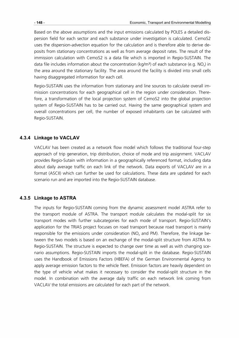
- 148 - Economic, Transport and Environmental Modelling
Based on the above assumptions and the input emissions calculated by POLES a detailed dis-
persion field for each sector and each substance under investigation is calculated. CemoS2
uses the dispersion-advection equation for the calculation and is therefore able to derive de-
posits from stationary concentrations as well as from average deposit rates. The result of the
immission calculation with CemoS2 is a data file which is imported in Regio-SUSTAIN. The
data file includes information about the concentration (kg/m³) of each substance (e.g. NOx) in
the area around the stationary facility. The area around the facility is divided into small cells
having disaggregated information for each cell.
Regio-SUSTAIN uses the information from stationary and line sources to calculate overall im-
mission concentrations for each geographical cell in the region under consideration. There-
fore, a transformation of the local projection system of CemoS2 into the global projection
system of Regio-SUSTAIN has to be carried out. Having the same geographical system and
overall concentrations per cell, the number of exposed inhabitants can be calculated with
Regio-SUSTAIN.
4.3.4 Linkage to VACLAV
VACLAV has been created as a network flow model which follows the traditional four-step
approach of trip generation, trip distribution, choice of mode and trip assignment. VACLAV
provides Regio-Sutain with information in a geographically referenced format, including data
about daily average traffic on each link of the network. Data exports of VACLAV are in a
format (ASCII) which can further be used for calculations. These data are updated for each
scenario run and are imported into the Regio-SUSTAIN database.
4.3.5 Linkage to ASTRA
The inputs for Regio-SUSTAIN coming from the dynamic assessment model ASTRA refer to
the transport module of ASTRA. The transport module calculates the modal-split for six
transport modes with further subcategories for each mode of transport. Regio-SUSTAIN’s
application for the TRIAS project focuses on road transport because road transport is mainly
responsible for the emissions under consideration (NOx and PM). Therefore, the linkage be-
tween the two models is based on an exchange of the modal-split structure from ASTRA to
Regio-SUSTAIN. The structure is expected to change over time as well as with changing sce-
nario assumptions. Regio-SUSTAIN imports the modal-split in the database. Regio-SUSTAIN
uses the Handbook of Emissions Factors (HBEFA) of the German Environmental Agency to
apply average emission factors to the vehicle fleet. Emission factors are heavily dependent on
the type of vehicle what makes it necessary to consider the modal-split structure in the
model. In combination with the average daily traffic on each network link coming from
VACLAV the total emissions are calculated for each part of the network.
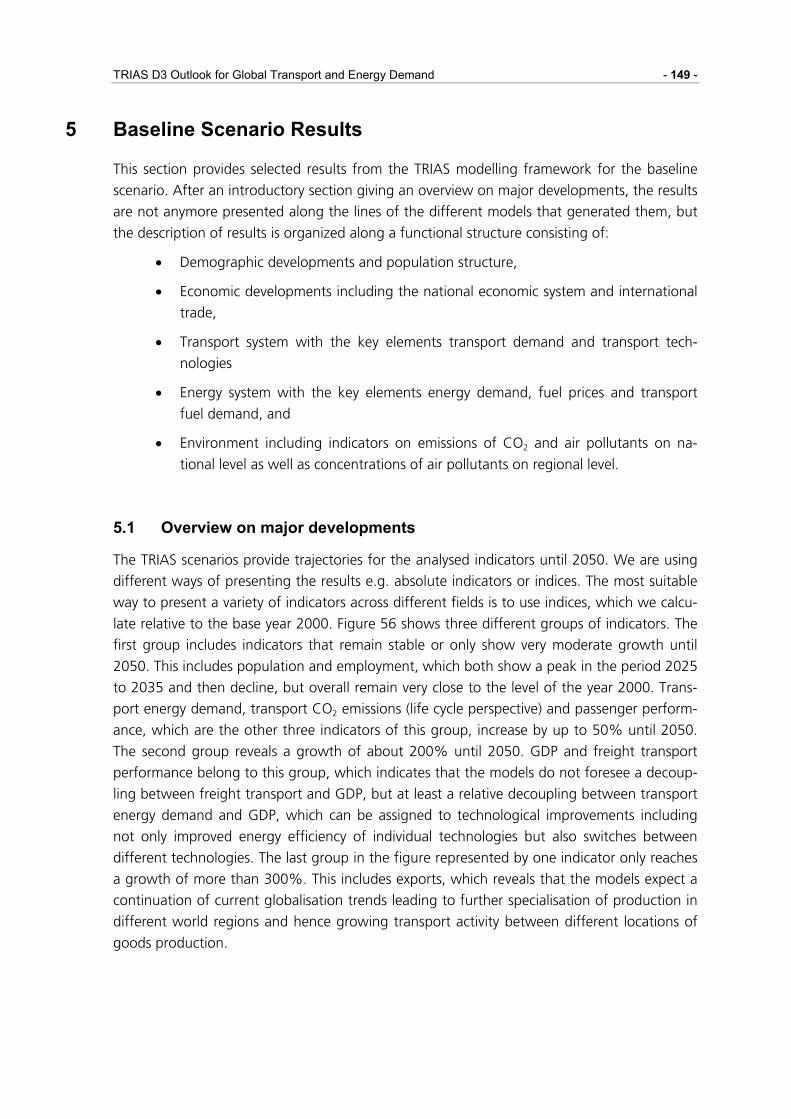
TRIAS D3 Outlook for Global Transport and Energy Demand - 149 -
5 Baseline Scenario Results
This section provides selected results from the TRIAS modelling framework for the baseline
scenario. After an introductory section giving an overview on major developments, the results
are not anymore presented along the lines of the different models that generated them, but
the description of results is organized along a functional structure consisting of:
• Demographic developments and population structure,
• Economic developments including the national economic system and international
trade,
• Transport system with the key elements transport demand and transport tech-
nologies
• Energy system with the key elements energy demand, fuel prices and transport
fuel demand, and
• Environment including indicators on emissions of CO2 and air pollutants on na-
tional level as well as concentrations of air pollutants on regional level.
5.1 Overview on major developments
The TRIAS scenarios provide trajectories for the analysed indicators until 2050. We are using
different ways of presenting the results e.g. absolute indicators or indices. The most suitable
way to present a variety of indicators across different fields is to use indices, which we calcu-
late relative to the base year 2000. Figure 56 shows three different groups of indicators. The
first group includes indicators that remain stable or only show very moderate growth until
2050. This includes population and employment, which both show a peak in the period 2025
to 2035 and then decline, but overall remain very close to the level of the year 2000. Trans-
port energy demand, transport CO2 emissions (life cycle perspective) and passenger perform-
ance, which are the other three indicators of this group, increase by up to 50% until 2050.
The second group reveals a growth of about 200% until 2050. GDP and freight transport
performance belong to this group, which indicates that the models do not foresee a decoup-
ling between freight transport and GDP, but at least a relative decoupling between transport
energy demand and GDP, which can be assigned to technological improvements including
not only improved energy efficiency of individual technologies but also switches between
different technologies. The last group in the figure represented by one indicator only reaches
a growth of more than 300%. This includes exports, which reveals that the models expect a
continuation of current globalisation trends leading to further specialisation of production in
different world regions and hence growing transport activity between different locations of
goods production.

- 150 - Baseline Scenario Results
Overview on major developments in the EU27
0
50
100
150
200
250
300
350
400
450
2000 2004 2008 2012 2016 2020 2024 2028 2032 2036 2040 2044 2048
Ind
ex [
year
200
0 =
100
]
Population
GDP
Exports
Employment
Freight performance
Passenger performance
Transport energy demand
Transport emiss ions CO2
Figure 56: Major developments in the transport-energy-economic system of the EU27
Taking a closer look at indicators of the transport and energy system in Figure 57 we can
observe that for both freight and passenger transport the volumes grow slower then the per-
formance, which indicates that travel distances continue to grow, and in particular for pas-
senger transport this is the most relevant driver of continued growth. Despite stabilisation of
the population the car fleet continues to grow significantly. One major reason is the catch-
ing-up of the new EU member states joining the EU in the years 2004 and 2007 in terms of
car-ownership. Further in some countries income continues to grow strongly, which is one of
the strongest drivers of car purchase, and finally it seems that ASTRA generating this indica-
tor is more on the optimistic side of forecasts for this indicator.
Consumption and prices of the currently dominating fuels, gasoline and diesel, behave dif-
ferently. For gasoline, we observe a strongly rising fuel price as well as a sharp reduction of
demand reaching about -50% until 2030, which is due to both improved efficiency and fuel
switch of cars. For diesel the fuel price increase is much more moderate. Efficiency improve-
ments of trucks and buses, which consume a large share of diesel, remain lower then for cars
such that together with the strong growth of freight transport diesel fuel demand doubles
until 2050. In addition part of the fuel switch of cars is from gasoline cars to diesel cars,
which also drives the growth of diesel fuel demand.

TRIAS D3 Outlook for Global Transport and Energy Demand - 151 -
Overview on major developments in the transport and energy system
0
50
100
150
200
250
300
350
2000 2004 2008 2012 2016 2020 2024 2028 2032 2036 2040 2044 2048
Inde
x (y
ear 2
000
= 10
0)Freight volume
Freight performance
Passenger volume
Passenger performanceCar fleet
Transport energy demand
Diesel fuel priceDiesel fuel demand
Gasoline fuel price
Gasoline fuel demand
Figure 57: Major developments in the transport and energy system of the EU27
5.2 Demographic Development
One of the main characteristics of the ASTRA population module (POP) is the independency
of outputs from other ASTRA modules. The POP module can be easily run as a stand-alone
model. It is mainly based on EUROSTAT data for fertility and death rates and the parameteri-
sation impacting the country-specific differences in death rates and the migration balance.
Future development of fertility and death rates are calibrated in order to fit EUROSTAT base-
line projections until 2050. Because of its independency on other modules and the different
scenario inputs the depicted results are valid for all TRIAS scenarios. In contrast to the Far in
excess of the EUROSTAT baseline projections the ASTRA POP module is able to simulate the
demographic changes per age cohort for each EU27 country.
Average annual population growth rates are presented in Table 40 for each country and total
EU27 population. All countries with positive population growth until 2050 are highlighted by
light green colour, countries with declining population by light orange colour. The POP mod-
ule estimates a decline of EU27 total population by annually –0.09% from 2005 to 2050. In
other words this annual decline leads to a EU27 population decrease of –3.4% or in total
numbers 16.6 Mio less people until 2050.

- 152 - Baseline Scenario Results
Table 40: Average yearly population growth rates Country 2005-2020 2021-2030 2031-2040 2041-2050 2005-2050 Total Change
AUT 0.19% 0.08% -0.06% -0.24% 0.01% 0.62% BLX 0.24% 0.20% 0.07% -0.03% 0.12% 6.21% DNK 0.16% 0.00% -0.02% -0.15% 0.01% 0.67% ESP 0.38% -0.03% -0.21% -0.42% -0.02% -0.91% FIN 0.20% 0.08% -0.13% -0.23% 0.00% 0.15% FRA 0.32% 0.24% 0.12% 0.02% 0.17% 8.95% GBR 0.30% 0.22% 0.10% -0.07% 0.14% 7.25% GER -0.01% -0.15% -0.32% -0.51% -0.20% -9.55% GRC 0.23% -0.10% -0.24% -0.38% -0.08% -3.78% IRL 0.99% 0.64% 0.45% 0.33% 0.58% 33.49% ITA 0.03% -0.22% -0.33% -0.46% -0.19% -9.14% NLD 0.34% 0.18% 0.05% -0.10% 0.13% 6.60% PRT 0.14% -0.07% -0.24% -0.43% -0.11% -5.21% SWE 0.39% 0.35% 0.23% 0.07% 0.25% 13.10% BLG -0.80% -0.94% -1.01% -0.94% -0.82% -33.62% CYP 1.02% 0.64% 0.35% 0.17% 0.54% 30.73% CZE -0.12% -0.29% -0.42% -0.45% -0.27% -12.62% EST -0.47% -0.42% -0.32% -0.33% -0.35% -16.22% HUN -0.25% -0.27% -0.31% -0.29% -0.25% -11.74% LAT -0.55% -0.44% -0.42% -0.35% -0.41% -18.42% LTU -0.42% -0.36% -0.31% -0.38% -0.34% -15.56% MLT 0.80% 0.47% 0.39% 0.24% 0.46% 25.81% POL -0.20% -0.23% -0.38% -0.41% -0.26% -12.36% ROM -0.48% -0.52% -0.62% -0.65% -0.50% -22.29% SLO 0.08% -0.10% -0.16% -0.32% -0.09% -4.57% SVK -0.12% -0.21% -0.36% -0.48% -0.25% -11.62%
Total EU27 0.10% -0.04% -0.17% -0.29% -0.07% -3.40% Source: ASTRA (2007)
Overall 16 countries are losing to some extent significantly population. In relative terms espe-
cially Eastern European members of the EU are affected by population decrease, while most
Western European member states are characterised by stagnating or even slightly growing
population. German and Italian population decrease most significantly by –9.6% and -7.7%.
Besides Slovenia all Eastern European member states with negative growth rates even outper-
form these relative decreases. Outstanding Bulgarian, Romanian and the Baltic states popula-
tion decrease significantly by –15.6% (Lithuania) up to –33.6% (Bulgaria). Most of these
countries lose population due to recent and prospectively expected high emigration rates
compared with immigration. Additionally most countries losing population suffer among the
ageing society problem. Old vintages with high birth rates are in many countries already re-
tired and finally more deaths compared with births lead to decreasing population. In contrast
Ireland, Cyprus and Malta denote high positive population growth rates up to +33.5% (Ire-
land) until 2050. Similar to the countries that are losing most population in relative terms
these countries benefit most from expected high immigration rates and therefore positive
migration balances.
Figure 58 underlines the problem of ageing society in EU27. The age group 65 plus indicated
as “Retired Persons” in the following figure increases by nearly +48.6% until 2050 compared
with 2005. Especially the decades from 2010 to 2040 are characterised by strong growth of
persons older than 65 due to high birth rates in the respective years while the number of
retired persons is stagnating in the last decade from 2040 to 2050. Labour force is decreas-

TRIAS D3 Outlook for Global Transport and Energy Demand - 153 -
ing by –11.9% until 2050 suffering among the transition of people in the “Retired Persons”
class and decreasing children numbers by –16.9%.
Demographic development in EU27
70
80
90
100
110
120
130
140
150
160
2005 2010 2015 2020 2025 2030 2035 2040 2045 2050
[Inde
x 20
05 =
100
]
Children Labour Force Retired Total Population
Figure 58: Demographic development in EU27
Share of Age Classes on Total Population in EU27
0%
1%
2%
3%
4%
5%
6%
7%
8%
9%
0 to 4
5 to 9
10 to
14
15 to
19
20 to
24
25 to
29
30 to
34
35 to
39
40 to
44
45 to
49
50 to
54
55 to
59
60 to
64
65 to
69
70 to
74
75 to
79
80 pl
us
2005 2050
Figure 59: Share of age classes on total population in EU27

- 154 - Baseline Scenario Results
Figure 59 presents a more detailed picture of prospective demographic structure in EU27.
The significant increase of the oldest age groups, especially the group 80 years plus, indicates
the observed increasing life expectancy in EU27.
The following Figure 60 pictures demographic trends of selected EU27 countries. Develop-
ment of the age cohorts children (0 to 17 years), labour force (18 to 64 years) and retired (65
years plus) are presented for Germany (GER), Poland (POL), Spain (ESP) and Romania (ROM).
All countries show the ageing society problem with more or less significantly increasing
population in retirement and decreasing numbers of children. Spain is characterised by a
strong increase of retired persons after 2020. The total number of retired persons is nearly
doubling until 2050. The same but slightly less worrying trend is visible in Poland starting 8
years earlier in 2012. This trend is influenced by high birth numbers in Poland in the period
from 1946 to 1960.
The demographic development in Romania shows a similar trend. Nevertheless the develop-
ment is special compared with the other countries. High emigration rates of people in work-
ing age lead to significantly decreasing birth numbers. In contrast to Spain and Poland the
growth of the age group older than 65 is not as strong, but the high emigration rates of
people in working age and strong decline of children lay a burden on the Romanian econ-
omy. Demographic trends estimated for Germany indicate also a relatively strong increase of
retired persons until 2035 followed by 15 years impacted by low birth numbers in the years
1970 to 1985. Birth rates are only slightly decreasing compared to Poland and Romania but
affect the total population development also negative.
Demographic Changes in Selected EU Countries
40
60
80
100
120
140
160
180
200
220
2005 2010 2015 2020 2025 2030 2035 2040 2045 2050
[Inde
x 20
05 =
100
]
Children GERLabour Force GERRetired GERChildren POLLabour Force POLRetired POLChildren ESPLabour Force ESPRetired ESPChildren ROMLabour Force ROMRetired ROM
Figure 60: Demographic changes in selected EU countries
Table 41 gives an overview on the demographic trends assessed for all EU27 countries for the
years 2030, 2040 and 2050. In general, the problem of ageing society can be observed in all
TRIAS D3 Outlook for Global Transport and Energy Demand - 155 -
countries. The age groups older than 65 years denote the highest growth while for nearly all
countries the numbers of births decline significantly compared with the base year 2005.
Table 41: Demographic changes per age class
0 to 17 18-64 65 plus 0 to 17 18-64 65 plus 0 to 17 18-64 65 plusAUT 92.3 97.8 140.3 92.3 92.8 156.3 89.7 91.7 148.6 BLX 99.3 100.7 132.7 100.8 99.4 139.8 100.6 99.9 136.5 DNK 93.1 98.0 135.9 96.7 94.0 146.9 95.6 94.3 136.8 ESP 93.3 98.3 148.0 83.0 87.8 189.0 82.6 79.5 197.8 FIN 99.0 97.3 142.7 97.9 97.0 135.7 93.0 95.9 132.1 FRA 100.0 101.4 141.4 100.9 100.4 152.3 100.3 101.0 151.6 GBR 96.4 104.1 135.2 97.1 101.7 151.1 95.4 102.1 146.5 GER 86.9 93.8 129.9 85.2 87.6 138.5 83.2 84.9 121.9 GRC 84.4 97.6 136.0 77.2 89.8 157.7 73.4 82.6 166.0 IRL 116.7 118.1 169.9 115.3 119.3 217.3 121.8 117.1 256.1 ITA 89.3 94.1 120.4 82.7 86.5 135.0 79.4 80.9 134.4 NLD 94.9 96.7 168.7 97.6 93.8 181.3 98.8 94.7 168.8 PRT 82.3 101.1 128.6 76.9 92.8 156.4 72.6 85.5 166.1 SWE 103.1 107.6 127.2 104.2 108.4 138.8 104.0 109.6 139.3 BLG 66.1 78.3 104.0 54.6 72.5 93.3 48.7 62.9 96.4 CYP 86.2 125.5 184.1 82.8 124.5 229.9 78.8 123.4 260.5 CZE 76.3 92.7 137.4 68.1 88.1 143.1 63.5 80.1 160.5 EST 71.8 97.0 85.7 61.0 95.4 88.6 56.5 86.7 106.8 HUN 76.9 91.8 125.6 71.2 87.7 132.1 68.1 82.0 144.0 LAT 69.8 90.0 102.8 59.5 90.2 93.5 55.5 84.2 102.7 LTU 63.8 95.2 111.3 56.5 91.4 119.3 51.8 84.5 132.3 MLT 100.2 122.4 124.1 96.9 126.1 141.9 93.8 125.2 165.9 POL 73.8 90.4 157.8 66.3 88.0 155.8 62.5 79.7 176.6 ROM 65.4 89.2 117.8 56.1 81.5 128.6 51.2 71.5 143.1 SLO 71.8 98.1 145.5 63.0 94.4 162.6 58.4 87.8 177.6 SVK 65.0 95.3 158.9 56.6 92.5 161.8 51.9 83.7 182.4
2030 2040 2050Country
Source: ASTRA (2007)
Many EU27 countries recognised the negative demographic trend and the arising burden on
the national economies. Politicians attached higher value to family issues in order to stop the
negative trend. Nevertheless the results highlight that demographic development and the
attempt of regulating the future demographic structure is a long-term process. Increasing
birth rates due to family-friendly policy impact the economy only earliest decades later when
children enter the labour market.
5.3 Economic Development
Basically ASTRA calculates the economic development of the European countries endoge-
nously, i.e. GDP the leading indicator to measure economic development is derived from a
number of causal relationships of ASTRA. For the purpose of harmonisation with other Euro-
pean studies parameters of these causal relationships can be adapted to provide GDP devel-
opments that are consistent with the development in the other studies. This does neither
mean that the GDP development of ASTRA is exactly the same as the one in the other studies
nor does it mean that it is taken exogenously as it still depends on the causal relationships
implemented in ASTRA. In particular this is important for the policy analysis, because only
when ASTRA endogenously calculates GDP, it is feasible to capture macroeconomic growth
impacts of the policies.
- 156 - Baseline Scenario Results
In the case of TRIAS the GDP development of ASTRA was adapted to fit to the baseline sce-
nario of the European ADAM project (http://www.adamproject.eu/). For most of the coun-
tries it was achieved to have a deviation of +/-20 % to the ADAM baseline in the year 2050.
Figure 61 presents the development of selected major economic indicators for the EU27
group of countries. GDP grows from the year 2000 by about 185 % until the year 2050,
which is equivalent to an annual growth of a bit more than +2 %. Private consumption fol-
lows nearly the same growth path, while exports and investments increase significantly
stronger than GDP reaching +290 % for investments and +310 % for exports. This is equiva-
lent to an annual growth of about +2.7 % for investments and +2.8 % for exports. The tra-
jectory for total factor productivity (TFP) represents only an approximation since this indicator
is calculated on country level based on sectoral inputs it is not possible to present an exact
value for the EU27 as this involves some weighting process (while for GDP and the other pre-
vious monetary indicators the EU27 value can be added up across the 27 countries to get the
EU27 value). The weighted indicator for TFP increases by +170 % until 2050, which still
makes it the largest contributor to growth of GDP on the supply side. The only indicator that
remains nearly stable over the whole time horizon is employment, For employment we ob-
serve an annual growth of close to +0.4 % until 2030 and an annual decline of a bit above -
0.4 % for the period 2030 until 2050. Since, population declines slightly stronger this implies
a slight increase of the activity rate of the population.
Overview on major economic developments for EU27
0
50
100
150
200
250
300
350
400
450
2000 2004 2008 2012 2016 2020 2024 2028 2032 2036 2040 2044 2048
GDP
Consumption
Investments
Exports
Gross capital stock
Total factor productivity
Gross value-added
Employment
Figure 61: Overview on major economic trajectories for EU27
Countrywise GDP growth of the EU15 countries is presented in Figure 62 and for the
EU12+2 countries in Figure 63. Overall the group of EU12 countries grows significantly
stronger revealing an annual growth of +2.8 % compared with +2 % of the group of EU15
countries. Partially this documents the catch-up of these countries, but on the other hand it is
also a mathematical artefact as the base value to calculate percentage changes is much
smaller for EU12 countries then for EU15 countries. In such cases it is even possible that ab-
solute growth could be smaller for those countries, which reveal a higher percentage growth.
This is not the case here, as the share of GDP of the EU15 countries on total GDP of EU27

TRIAS D3 Outlook for Global Transport and Energy Demand - 157 -
decreases from 95% in 2000 to about 93% in 2050. The ranking of countries in terms of
GDP remains mostly stable though some stronger growing countries like Spain and the
United Kingdom increase their relative importance, while Germany and France slightly loose
importance. In the case of France, the growth potential should be underestimated by ASTRA
in TRIAS.
GDP development in the EU15 countries [Mio*EURO]
0
2,000,000
4,000,000
6,000,000
8,000,000
10,000,000
12,000,000
14,000,000
16,000,000
18,000,000
20,000,000
2000 2004 2008 2012 2016 2020 2024 2028 2032 2036 2040 2044 2048
Sw eden
Portugal
Netherlands
Italy
Ireland
Greece
Germany
United Kingdom
France
Finland
Spain
Denmark
Belgium+Luxemburg
Austria
Figure 62: GDP trajectories for the individual EU15 countries
GDP development in the EU12 + 2 countries [Mio*EURO]
0
500,000
1,000,000
1,500,000
2,000,000
2,500,000
3,000,000
2000 2004 2008 2012 2016 2020 2024 2028 2032 2036 2040 2044 2048
Slovakia
Slovenia
Romania
Poland
Malta
Lithuania
Latvia
Hungary
Estonia
Czech Republic
Cyprus
Bulgaria
Norw ay
Sw itzerland
Figure 63: GDP trajectories for the individual EU12+2 countries

- 158 - Baseline Scenario Results
Exports constitute one of the most important drivers of economic growth. Figure 64 presents
the growth of exports from goods sectors of the EU27 and Figure 65 the growth of the ser-
vice sectors. In particular the growth of the goods sectors is relevant as it generates freight
transport in ASTRA, though one has to take into account that these are monetary values,
which do not directly translate into volumes of goods transport. The four strongest export
sectors of the EU27 remain in their ranking with vehicles being the largest export sector and
then chemicals, electronics and industrial machinery. In terms of growth percentages be-
tween 2010 and 2050 the ranking is different: communication services grow strongest fol-
lowed by computers, electronics and catering services, the latter reflecting the growth in
tourism.
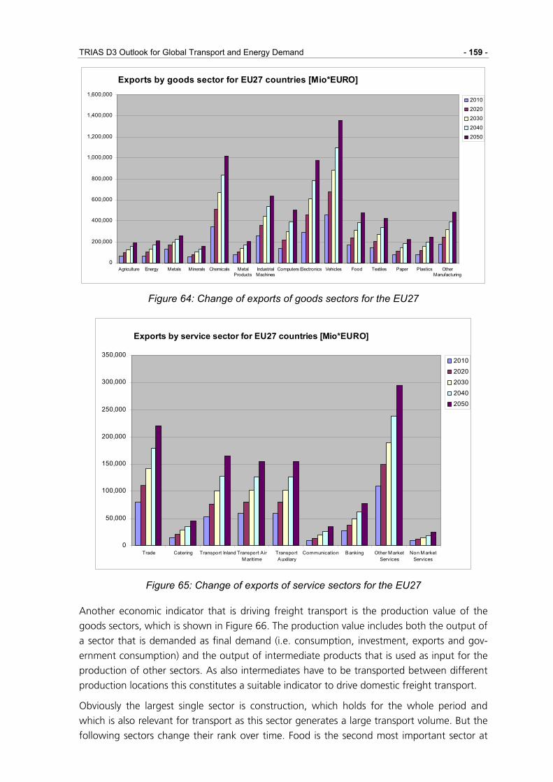
TRIAS D3 Outlook for Global Transport and Energy Demand - 159 -
Exports by goods sector for EU27 countries [Mio*EURO]
0
200,000
400,000
600,000
800,000
1,000,000
1,200,000
1,400,000
1,600,000
Agriculture Energy Metals Minerals Chemicals MetalProducts
IndustrialMachines
Computers Electronics Vehicles Food Textiles Paper Plastics OtherManufacturing
2010
2020
2030
2040
2050
Figure 64: Change of exports of goods sectors for the EU27
Exports by service sector for EU27 countries [Mio*EURO]
0
50,000
100,000
150,000
200,000
250,000
300,000
350,000
Trade Catering Transport Inland Transport A irM aritime
TransportAuxiliary
Communication Banking Other M arketServices
Non M arketServices
2010
2020
2030
2040
2050
Figure 65: Change of exports of service sectors for the EU27
Another economic indicator that is driving freight transport is the production value of the
goods sectors, which is shown in Figure 66. The production value includes both the output of
a sector that is demanded as final demand (i.e. consumption, investment, exports and gov-
ernment consumption) and the output of intermediate products that is used as input for the
production of other sectors. As also intermediates have to be transported between different
production locations this constitutes a suitable indicator to drive domestic freight transport.
Obviously the largest single sector is construction, which holds for the whole period and
which is also relevant for transport as this sector generates a large transport volume. But the
following sectors change their rank over time. Food is the second most important sector at

- 160 - Baseline Scenario Results
the beginning in 2010, but vehicles take over this role at 2020. Chemicals increase their rank
and become the fourth largest sector in terms of production value after 2030. In terms of
growth percentages the ranking of the most dynamic sectors is computers with over +300 %
between 2010 and 2050 followed by electronics (+275 %) and vehicles (+246 %). Including
service sectors two of them would also belong to the most dynamic sectors: other market
services (+281 %) as well as air and maritime transport services (+245 %).
Production value by goods sector for EU27 countries [Mio*EURO]
0
500,000
1,000,000
1,500,000
2,000,000
2,500,000
3,000,000
3,500,000
4,000,000
4,500,000
Agriculture Energy Metals Minerals Chemicals MetalProducts
IndustrialMachines
Computers Electronics Vehicles Food Textiles Paper Plastics OtherManufacturing
Construction
2010
20202030
2040
2050
Figure 66: Change of production value of goods sectors in EU27
In terms of employment by sector the picture differs significantly from the one of production
value as shown in Figure 67 for goods sectors and in Figure 68 for service sectors. The main
similarity is that other market services constitute by far the largest sector. But in contrast to
production value only for a few sectors dynamic growth can be observed, and is all cases this
is not maintained over the whole period between 2010 and 2050. Employment in other mar-
ket services grows until 2040 and then reduces; trade, after 2030 the second largest sector,
remains more or less stable, while non-market services (i.e. mainly public authorities and pub-
lic services) decline and loose their second most important position in 2030. For construction,
the fourth most relevant sector for employment, growth can be observed until 2030 and
afterwards employment reduces. Agriculture looses employment until 2020 and then stabi-
lizes. The most dynamic and relevant sectors are vehicles with a growth of +39 % and food
with +32 % between 2010 and 2050.

TRIAS D3 Outlook for Global Transport and Energy Demand - 161 -
Employment by goods sector for EU27 countries [Persons]
0
5,000,000
10,000,000
15,000,000
20,000,000
25,000,000
Agriculture Energy Metals Minerals Chemicals MetalProducts
IndustrialMachines
ComputersElectronics Vehicles Food Textiles Paper Plastics OtherManufacturing
Construction
2010
2020
2030
2040
2050
Figure 67: Change of employment in goods sectors of EU27
Employment by service sector for EU27 countries [Persons]
0
10,000,000
20,000,000
30,000,000
40,000,000
50,000,000
60,000,000
70,000,000
Trade Catering Transport Inland Transport A irM aritime
TransportAuxiliary
Communication Banking Other M arketServices
Non M arketServices
2010
2020
2030
2040
2050
Figure 68: Change of employment in service sectors of EU27
Figure 69 presents a different view on the trajectories of employment by sector in the EU27
countries. In this view the strong reduction of agricultural employment until 2020 due to the
restructuring of agriculture in the new EU member states of the years 2004 and 2007 be-
comes obvious. Also the continuous decline of employment in the government sector is ap-
parent, which is fostered by concepts like the lean state and the continued privatisation of
former governmental activities like health care (e.g. hospitals) or education. Also the two
large sectors construction and other market services experiencing growth until 2030-2035
and afterwards decline can be identified easily.

- 162 - Baseline Scenario Results
Development of employment by goods sector in EU27 [Persons]
0
10,000,000
20,000,000
30,000,000
40,000,000
50,000,000
60,000,000
70,000,000
80,000,000
90,000,000
2000 2004 2008 2012 2016 2020 2024 2028 2032 2036 2040 2044 2048
ConstructionOther ManufacturingPlasticsPaper
TextilesFoodVehiclesElectronicsComputers
Industrial MachinesMetal ProductsChemicalsMineralsMetals
EnergyAgriculture
Development of employment by service sector in EU27 [Persons]
0
20,000,000
40,000,000
60,000,000
80,000,000
100,000,000
120,000,000
140,000,000
160,000,000
2000 2004 2008 2012 2016 2020 2024 2028 2032 2036 2040 2044 2048
Non Market Services
Other Market Services
Banking
CommunicationTransport Auxiliary
Transport Air MaritimeTransport Inland
CateringTrade
Figure 69: Trajectories of employment by sectors in EU27
Another element of the economic system that is related to transport is investments into
transport infrastructure and into vehicles. These are presented in Figure 70 differentiated into
EU12 and EU15. The total of all curves represents total transport investment in EU27. It is
important to notice that investment into vehicles grow much stronger than into infrastruc-
ture. Investments into vehicles increase only slightly slower than the total investments in
these regions, while transport infrastructure investments for EU15 grow at a similar pace as
EU15 GDP, while for the EU12 the transport infrastructure investments grow even signifi-
cantly slower than GDP. In other words, for EU15 the share of transport infrastructure in-
vestments on GDP remains more or less constant, while this share is declining for EU12 coun-
tries.
Transport investment in different categories for EU12 and EU15 [Mio*EURO]
0
100,000
200,000
300,000
400,000
500,000
600,000
700,000
2000 2004 2008 2012 2016 2020 2024 2028 2032 2036 2040 2044 2048
Infrastructure EU15
Infrastructure EU12
Vehicles EU15
Vehicles EU12
Figure 70: Trajectories of different transport related investments in EU12 and EU15

TRIAS D3 Outlook for Global Transport and Energy Demand - 163 -
5.4 Transport System Trends
The following graphs summarise the base trend of the passenger, freight traffic and vehicle
fleet composition in the baseline scenario.
ASTRA Transport System Trends
The trend of personal mobility shows an increment at different speed when EU15 and more
recent EU Member States are considered. The latter are forecasted to grow faster in the near
future as impact of higher incomes and motorisation rates. However, the expected decreas-
ing of population in the Eastern Europe countries partially offsets these determinants result-
ing in a diminished growth rates and finally also in a reducing mobility in absolute terms with
respect to the maximum level reached before 2040. Even if the path is different, at the end
of the simulation period the same relative increment is forecast for both areas: 50% more
passengers-km, which means an average growth rate of 0.8% per year. In the recent years
passenger traffic has grown by 1.8% per year1, therefore the TRIAS baseline forecast a slow
down of personal mobility.
Total passenger traffic index (year 2000 = 100)
0
20
40
60
80
100
120
140
160
180
2000
2002
2004
2006
2008
2010
2012
2014
2016
2018
2020
2022
2024
2026
2028
2030
2032
2034
2036
2038
2040
2042
2044
2046
2048
2050
EU15 EU12
Figure 71: Baseline trend of total pkm
The difference between the two groups of countries is more significant looking at the mobil-
ity of goods, which in the Eastern Europe countries is expected to increase more significantly
due to the higher economic development rates. For the EU15 countries, the TRIAS baseline
foresee that in the year 2050 the amount of tonnes-km will be tripled with respect to the
year 2000. This forecast corresponds to an average growth rate of 2.2% per year, which is in
1 Source: EU Energy and Transport in Figures – Statistical Pocketbook 2006. All observed data
quoted below in this paragraph is drawn from EU Energy and Transport in Figures unless di-versely specified.
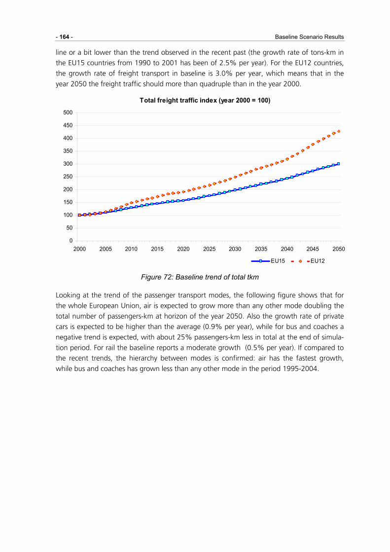
- 164 - Baseline Scenario Results
line or a bit lower than the trend observed in the recent past (the growth rate of tons-km in
the EU15 countries from 1990 to 2001 has been of 2.5% per year). For the EU12 countries,
the growth rate of freight transport in baseline is 3.0% per year, which means that in the
year 2050 the freight traffic should more than quadruple than in the year 2000.
Total freight traffic index (year 2000 = 100)
0
50
100
150
200
250
300
350
400
450
500
2000 2005 2010 2015 2020 2025 2030 2035 2040 2045 2050
EU15 EU12
Figure 72: Baseline trend of total tkm
Looking at the trend of the passenger transport modes, the following figure shows that for
the whole European Union, air is expected to grow more than any other mode doubling the
total number of passengers-km at horizon of the year 2050. Also the growth rate of private
cars is expected to be higher than the average (0.9% per year), while for bus and coaches a
negative trend is expected, with about 25% passengers-km less in total at the end of simula-
tion period. For rail the baseline reports a moderate growth (0.5% per year). If compared to
the recent trends, the hierarchy between modes is confirmed: air has the fastest growth,
while bus and coaches has grown less than any other mode in the period 1995-2004.

TRIAS D3 Outlook for Global Transport and Energy Demand - 165 -
EU27 passenger traffic index, per mode (year 2000 = 100)
-
20
40
60
80
100
120
140
160
180
200
220
2000
2002
2004
2006
2008
2010
2012
2014
2016
2018
2020
2022
2024
2026
2028
2030
2032
2034
2036
2038
2040
2042
2044
2046
2048
2050
Car Bus Train Air
Figure 73: Baseline trend of Pass-km by mode of transport
The different trend of the modes brings to a modification of the mode split. Figure below
illustrates how the mode shares evolve in the baseline for the EU27.
EU27 Modal shares
73.2% 73.4% 74.5% 75.2% 75.7% 76.2% 76.6% 76.8% 77.0% 77.2% 77.0%
9.4% 8.8% 7.9% 7.2% 6.6% 6.2% 5.8% 5.5% 5.1% 4.8% 4.5%7.7% 8.0% 7.6% 7.4% 7.2% 7.0% 6.8% 6.7% 6.6% 6.5% 6.6%
6.1% 6.1% 6.4% 6.5% 6.7% 7.0% 7.2% 7.3% 7.5% 7.7% 8.1%3.6% 3.7% 3.7% 3.7% 3.7% 3.7% 3.7% 3.7% 3.7% 3.8% 3.8%
0%
10%
20%
30%
40%
50%
60%
70%
80%
90%
100%
2000
2005
2010
2015
2020
2025
2030
2035
2040
2045
2050
Car Bus Train Air Slow
Figure 74: Baseline trend of passenger mode split in the EU27 countries
The mode share of car and air is expected to grow. In particular, air becomes the second
transport mode in terms of passengers-km, overtaking bus and train. The former is the major
loser as its mode share is more than halved. Again these forecasts are reasonably consistent
with observed data. For instance, bus share was about 10% in the year 1995 and less than

- 166 - Baseline Scenario Results
9% in the year 2004, and in same period, rail share slightly fall from a bit more than 8% to
less than 8%.
Looking at the role of car on motorised land trips (i.e. excluding air trips), table below shows
that in all EU countries the share of passengers-km performed by car is expected to increase,
but in EU12 countries, where the share of car and the motorization rate at the year 2000 are
generally lower than in the EU15 countries, the growth rates are higher. It is remarkable that
this trend occurs even if the car cost is supposed to grow more than costs of other modes in
the simulated period (see chapter 3).
Table 42: Change of car share(1) in the EU27 countries in the baseline
Country 2000 (2) 2050 Var% 2000 - 2050 AUT 76% 86% 13.0%BLX 82% 89% 9.1%DNK 79% 88% 11.6%ESP 81% 89% 10.0%FIN 82% 89% 9.5%FRA 85% 90% 6.1%GBR 87% 87% 0.1%GER 84% 90% 6.8%GRC 76% 84% 10.5%IRL 72% 86% 18.9%ITA 83% 90% 7.8%NLD 85% 88% 2.9%PRT 82% 86% 5.7%SWE 80% 89% 10.5%BLG 27% 55% 99.7%CYP 48% 75% 54.9%CZE 73% 84% 15.0%EST 76% 86% 12.9%HUN 65% 75% 15.3%LAT 73% 80% 9.4%LTU 84% 88% 5.0%MLT 74% 87% 18.2%POL 78% 87% 12.1%ROM 22% 42% 87.0%SLO 85% 92% 8.1%SVK 69% 81% 18.7%
(1) Share computed on the car traffic measured in passengers-km with respect to total
traffic of motorised land modes (i.e. excluding air and slow modes)
(2) The data for the year 2000 concerns modelled shares not observed ones.
Also for freight transport, the foreseen baseline growth of modes is different (see figure 8).
Road is expected to grow faster than its competitors – rail and maritime – at a pace of about
2.7% per year. Rail growth should be slower than road’s but faster than maritime’s. In the
recent past maritime has actually shown larger growth rates than rail, so from this point of
view the TRIAS baseline introduces a break in the series. An explanation for this break is that

TRIAS D3 Outlook for Global Transport and Energy Demand - 167 -
in the ASTRA model, only intra-Europe transport demand is considered. In the model, the
economic development of the EU countries gives rise to an increment of transported goods.
Actually, part of the generated demand concerns trades with overseas countries and mari-
time statistics are affected by this trades, while ASTRA deal with the impact on intra-Europe
demand only.
EU27 freight traffic index, per mode (year 2000 = 100)
50
100
150
200
250
300
350
400
2000 2005 2010 2015 2020 2025 2030 2035 2040 2045 2050
Road Rail Ship
Figure 75: Baseline trend of Tonnes-km by mode of transport

- 168 - Baseline Scenario Results
EU27 Modal shares
50.3% 49.8% 48.3% 49.0% 50.3% 51.8% 53.5% 55.1% 56.8% 58.0% 59.6%
14.8% 15.1% 15.3% 15.3% 15.1% 15.1% 15.1% 15.1% 15.0% 15.0% 14.9%
34.9% 35.0% 36.4% 35.7% 34.6% 33.1% 31.4% 29.9% 28.2% 27.1% 25.5%
0%
10%
20%
30%
40%
50%
60%
70%
80%
90%
100%
2000
2005
2010
2015
2020
2025
2030
2035
2040
2045
2050
Road Rail Ship
Figure 76: Baseline trend of freight mode split in the EU27 countries
As a consequence of the different trend of the transport modes, mode shares change over
time in the TRIAS baseline as shown in figure 9. Rail maintains is share even if the road
freight grows much faster. As road and maritime usually are not direct competitors (road is
used on shorter distances and for smaller loads), the evolution of mode shares suggests a
double shift: from rail to road and from ship to rail. At the basis of this mode shift there is
the different development of the economic sectors. Coastal ships are mainly used for bulk
goods (oil products, irons, cereals, etc.) whose relevance on the intra-EU trade is decreasing
over time. Container ships are especially used to and from overseas, while within EU rail is an
alternative mode for this share of traffic, which is the fastest developing one. Therefore, the
TRIAS baseline suggests that the future freight demand will be larger and differently com-
posed, higher value goods will be a higher share of total traffic and therefore modes like rail
and especially road will be preferred to ship.
ASTRA Vehicle Fleet Trends
In comparison with results from previous ASTRA simulations the TRIAS baseline scenario
simulation comprise five new alternative car technologies in addition to five conventional car
categories. The following figures demonstrate the baseline scenario trends estimated by
ASTRA for car, bus and goods vehicle fleets and highlight the assessed technological devel-
opment in EU27.
Figure 77 provides an overview on the estimated vehicle fleet development in EU27 until
2050. Analysing the projections one has to take into account the different modelling mecha-
nisms for car, bus and goods vehicle fleets. In contrast to new bus, light and heavy duty vehi-
cle registrations the number of new registered passenger cars depends mainly on factors like
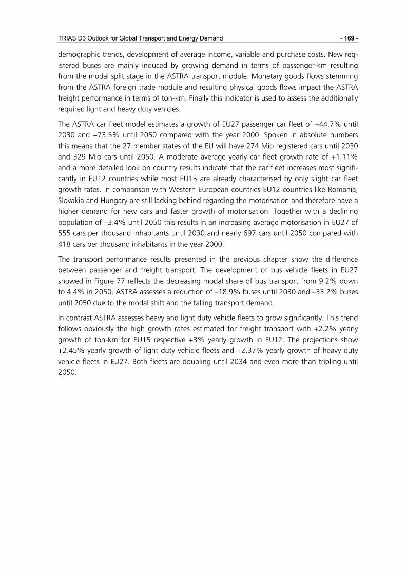
TRIAS D3 Outlook for Global Transport and Energy Demand - 169 -
demographic trends, development of average income, variable and purchase costs. New reg-
istered buses are mainly induced by growing demand in terms of passenger-km resulting
from the modal split stage in the ASTRA transport module. Monetary goods flows stemming
from the ASTRA foreign trade module and resulting physical goods flows impact the ASTRA
freight performance in terms of ton-km. Finally this indicator is used to assess the additionally
required light and heavy duty vehicles.
The ASTRA car fleet model estimates a growth of EU27 passenger car fleet of +44.7% until
2030 and +73.5% until 2050 compared with the year 2000. Spoken in absolute numbers
this means that the 27 member states of the EU will have 274 Mio registered cars until 2030
and 329 Mio cars until 2050. A moderate average yearly car fleet growth rate of +1.11%
and a more detailed look on country results indicate that the car fleet increases most signifi-
cantly in EU12 countries while most EU15 are already characterised by only slight car fleet
growth rates. In comparison with Western European countries EU12 countries like Romania,
Slovakia and Hungary are still lacking behind regarding the motorisation and therefore have a
higher demand for new cars and faster growth of motorisation. Together with a declining
population of –3.4% until 2050 this results in an increasing average motorisation in EU27 of
555 cars per thousand inhabitants until 2030 and nearly 697 cars until 2050 compared with
418 cars per thousand inhabitants in the year 2000.
The transport performance results presented in the previous chapter show the difference
between passenger and freight transport. The development of bus vehicle fleets in EU27
showed in Figure 77 reflects the decreasing modal share of bus transport from 9.2% down
to 4.4% in 2050. ASTRA assesses a reduction of –18.9% buses until 2030 and –33.2% buses
until 2050 due to the modal shift and the falling transport demand.
In contrast ASTRA assesses heavy and light duty vehicle fleets to grow significantly. This trend
follows obviously the high growth rates estimated for freight transport with +2.2% yearly
growth of ton-km for EU15 respective +3% yearly growth in EU12. The projections show
+2.45% yearly growth of light duty vehicle fleets and +2.37% yearly growth of heavy duty
vehicle fleets in EU27. Both fleets are doubling until 2034 and even more than tripling until
2050.
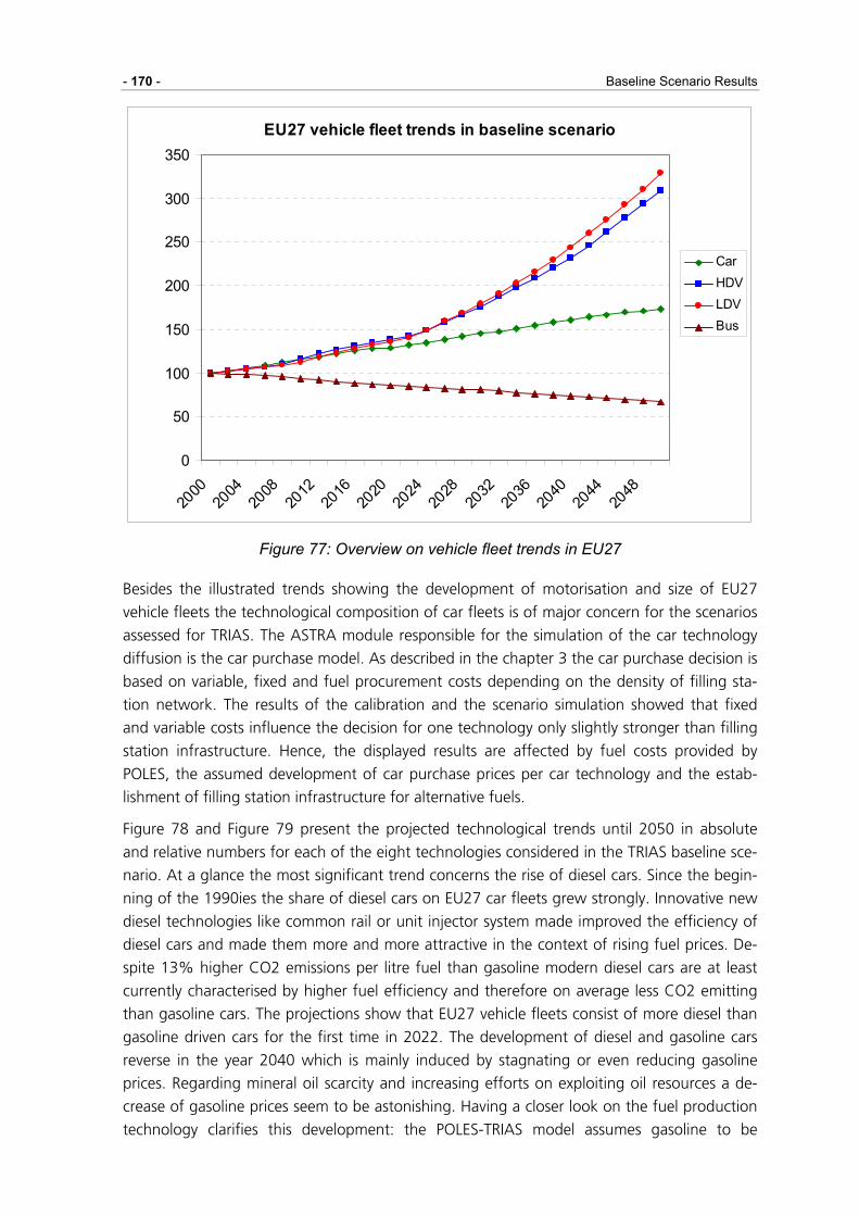
- 170 - Baseline Scenario Results
EU27 vehicle fleet trends in baseline scenario
0
50
100
150
200
250
300
350
2000
2004
2008
2012
2016
2020
2024
2028
2032
2036
2040
2044
2048
CarHDVLDVBus
Figure 77: Overview on vehicle fleet trends in EU27
Besides the illustrated trends showing the development of motorisation and size of EU27
vehicle fleets the technological composition of car fleets is of major concern for the scenarios
assessed for TRIAS. The ASTRA module responsible for the simulation of the car technology
diffusion is the car purchase model. As described in the chapter 3 the car purchase decision is
based on variable, fixed and fuel procurement costs depending on the density of filling sta-
tion network. The results of the calibration and the scenario simulation showed that fixed
and variable costs influence the decision for one technology only slightly stronger than filling
station infrastructure. Hence, the displayed results are affected by fuel costs provided by
POLES, the assumed development of car purchase prices per car technology and the estab-
lishment of filling station infrastructure for alternative fuels.
Figure 78 and Figure 79 present the projected technological trends until 2050 in absolute
and relative numbers for each of the eight technologies considered in the TRIAS baseline sce-
nario. At a glance the most significant trend concerns the rise of diesel cars. Since the begin-
ning of the 1990ies the share of diesel cars on EU27 car fleets grew strongly. Innovative new
diesel technologies like common rail or unit injector system made improved the efficiency of
diesel cars and made them more and more attractive in the context of rising fuel prices. De-
spite 13% higher CO2 emissions per litre fuel than gasoline modern diesel cars are at least
currently characterised by higher fuel efficiency and therefore on average less CO2 emitting
than gasoline cars. The projections show that EU27 vehicle fleets consist of more diesel than
gasoline driven cars for the first time in 2022. The development of diesel and gasoline cars
reverse in the year 2040 which is mainly induced by stagnating or even reducing gasoline
prices. Regarding mineral oil scarcity and increasing efforts on exploiting oil resources a de-
crease of gasoline prices seem to be astonishing. Having a closer look on the fuel production
technology clarifies this development: the POLES-TRIAS model assumes gasoline to be

TRIAS D3 Outlook for Global Transport and Energy Demand - 171 -
blended with lignocellulosic ethanol starting in 2030. As the production process of lignocellu-
losic ethanol is characterised by low costs (see Table 43), gasoline prices decline with increas-
ing shares of this kind of ethanol. The observed reversing trend is enabled by the car pur-
chase model structure even if it is controversial that old technologies might return in the fo-
cus as a kind of renaissance. The observed positive development of LPG car registrations in
Germany and many other countries are an example for old technologies - LPG cars entered
the first markets already in the 1970ies – that rebound as alternatives to other conventional
car technologies. Finally the assessment provides a share of diesel cars in EU27 car fleets of
39.6% in the year 2050.
Another interesting outcome of the baseline scenario is the estimated substitution process
from gasoline car with high cubic capacity to powerful motorised diesel cars, which is already
ongoing since the end of the 1990ies. The originally unattractive old diesel technology be-
came competitive to high-powered cars.
Car technology trends in EU27 - Baseline
0
50
100
150
200
250
300
350
1990
1994
1998
2002
2006
2010
2014
2018
2022
2026
2030
2034
2038
2042
2046
2050
H2BIOELCHYBLPGCNGDPC2DPC1GPC3GPC2GPC1
Figure 78: Passenger car technology trends in EU27
The baseline scenario identifies NGV (natural gas vehicles) as the most attractive alternative
car technology to car buyers in the mid term. Countries like Germany, Italy, Sweden, Austria
and UK currently support the diffusion of CNG cars into the markets and the improvement of
filling station infrastructure via action plans. This results in an EU27 share up to 12.9% in the
year 2024. In the following years CNG cars are estimated to lose share and end up at 7.2%
in 2050. The declining share from 2024 onwards is mainly caused by increasing natural gas
prices computed by the POLES-TRIAS model. Compared with other technologies like bioetha-
nol or conventional technology NGV loses attractiveness and the share declines. Regarding
the fleet share development of LPG one can say that the modern CNG technology is substi-
tuting the older LPG technology. The ASTRA model assesses a reduction of LPG share from
1.4% in 2005 to 0.8% in 2050. Cars driven with bioethanol (BIO) or E85 are projected to

- 172 - Baseline Scenario Results
have the second highest share of all alternative fuel cars in the baseline scenario. The market
share of bioethanol cars in EU27 is increasing and reaches a peak in the year 2032. In the
following decades the share is stagnating and ending in 5.4% in the year 2050.
The stagnating or even reversing trend observed for CNG and bioethanol driven cars is mainly
caused by increasing efficiency of gasoline cars. Caused by stagnating gasoline prices esti-
mated in POLES the fully developed technology attracts buyers and lead to a slightly recover-
ing share of at least small and partially medium sized gasoline cars. Nevertheless the share of
gasoline cars in EU27 declines with -28.2% significantly from 75.8% in the year 2000 down
to 47.6% in the year 2050.
EU27 development of car technologies
0%
5%
10%
15%
20%
25%
30%
35%
40%
45%
2000
2004
2008
2012
2016
2020
2024
2028
2032
2036
2040
2044
2048
GPC1GPC2GPC3DPC1DPC2CNGLPGHYBELCBIOH2
Figure 79: Share of passenger car technology in EU27
5.5 Energy System Trends
POLES Energy Demand
Without taking electricity and transformation system sector into account, the total energy
demand in EU27 can be expected to increase by a factor of 1.4 during the period 2006-
2050, which means 0.75% increase per year. Transportation is the most energy intensive
sector, of which the share of total demand increases from 39% in 2006 to 41% in 2050.
Residential sector share decreases from 23% in 2006 to 18.8% in 2050 while service sector
share increases from 10% in 2006 to 17% in 2050 (Figure 80).

TRIAS D3 Outlook for Global Transport and Energy Demand - 173 -
0
200
400
600
800
1000
1200
1400
1600
1800
2000
2006
2009
2012
2015
2018
2021
2024
2027
2030
2033
2036
2039
2042
2045
2048
Mto
e
Steel IndustryService SectorResidential SectorOther Industry w/ non energy useNon Metallic Mineral IndustryChemical Industry w/ FeedstockTransportAgriculture
Figure 80: EU27 total energy consumption (without electricity and transformation sector)
The fuel consumption of the industrialised countries (including CIS) can be expected to in-
crease by a factor of 1.4 during the period 2006-2050. The share of Europe in the world total
energy consumption will decrease from 27% to 22% during this period. In the developing
world, energy consumption will increase by a factor of 2.5 during the same period (Figure
81). China's share, which is the biggest among the developing world, will increase from 17%
in 2006 to 22% in 2050. In 2006, two-third of the consumption comes from the industrial-
ised countries while the remaining one-third comes from the developing world. By 2050, the
share of the consumption can be expected to reach a ratio of 50:50.
0
1
2
3
4
5
6
7
8
9
2006
2009
2012
2015
2018
2021
2024
2027
2030
2033
2036
2039
2042
2045
2048
Gto
e
EuropeNorth AmericaJapan-PacificCISLatin AmericaAfricaMiddle EastChinaIndiaRest Asia
Figure 81: Total world energy consumption by region (without electricity and transforma-tion system)

- 174 - Baseline Scenario Results
Biofuels
The production costs increase for biofuels of the 1st generation and decline for biofuels of the
2nd generation (Table 43). Production costs rise due to increasing feedstock costs, which are
not compensated by learning effects. A decrease in production costs of first generation bio-
fuels due to the learning effect was not taken into account as they are considered limited
and lie within the range of uncertainties. Biodiesel production is a mature technology and
even though bioethanol production in Europe is lagging behind biodiesel in terms of produc-
tion volumes, the technology can be considered mature as well, especially when taking into
account the global deployment of bioethanol. Besides, economies of scale due to larger plant
sizes will be counteracted by more complicated logistics and increased transport costs.
Table 43: Biofuel production costs Production costs [€/toe]
Pathways 2010 2020 2030 2040 2050
Bioethanol from Wheat 628.0 705.2 731.5 750.0 764.7
Bioethanol from Sugarbeet 642.4 721.3 748.3 767.1 782.2
Biodiesel from Rapeseed 726.8 700.7 739.9 762.4 809.7
Biodiesel from Sunflower 713.4 696.1 733.8 756.7 802.4
Lignocellulosic ethanol (straw) 928.6 818.5 736.1 733.2 743.7
Synthetic diesel (farmed wood) 1118.5 1014.7 924.6 894.2 891.5
Contrarily, the production costs of the 2nd generation of biofuels decrease. For 2nd generation
of biofuels, technology learning plays an important role for the market introduction. These
are expected to be technically available on commercial scale between 2010 and 2020, al-
though their commercial viability will depend on how competitive their prices will be. Impor-
tant cost reductions can be expected both in terms of the production process due to econo-
mies of scale and more mature technologies and in terms of the feedstock, as current crops
are not yet optimised for their energy content.
With the above cost reductions, production costs of 2nd generation ethanol reach that of
conventional ethanol between 2020 and 2030, while synthetic diesel (BtL) remains more ex-
pensive with about 900 €/toe.
In the base scenario, production costs of biofuels remain above costs of fossil fuel, which is
around 500 €/toe in 2010 and is assumed to be around 700 €/toe in 2050. Therefore, biofu-
els enter the market due to the quota set on a Member State level. In the base scenario, the
quota for the country groups 1 and to 2 is assumed to be 5.75%, respectively 2.35% for the
countries of country group 3 and 4.
The biofuel production increases very rapidly until around 2012 and remains than on this
level until 2030 (Figure 82). This is due to the assumption that the incentive for investors to
build additional production capacity decreases the closer they come to the equilibrium point.
After 2030 a further increase is expected due to the introduction of 2nd generation biofuels.

TRIAS D3 Outlook for Global Transport and Energy Demand - 175 -
In the case of biodiesel, for example, the model predicts reduced growth rates already
around 2012, while this occurs for bioethanol only about one decade later. Up to today, bio-
diesel dominates the EU biofuel market with a share of more than 80% (unlike the US and
Brazil where ethanol clearly dominates [F.O. Licht, 2006]). In the base scenario the biodiesel
production increases from 3.4 mill toe in 2006 to 8.5 mill toe in 2010.
Biofuel production
0
2
4
6
8
10
12
14
16
18
20
1990
1994
1998
2002
2006
2010
2014
2018
2022
2026
2030
2034
2038
2042
2046
2050
mill toe
BTLCelluEthanolBiodieselBioethanol
Figure 82: Biofuel production in the base scenario
The base scenario project that the trend of an increase of biodiesel production is likely to not
continue in the longer term. Due to lower production costs and in particular lower feedback
on feedstock prices, bioethanol production is projected to increase at a much faster rate than
biodiesel. The fast uptake of ethanol will slow down once additional distribution and adapta-
tion costs are required due to problems in blending ethanol above a certain low share, but
cannot reverse the trend.
2nd generation biofuels are projected to enter the market after 2030 when production costs
of ligno-cellulosic ethanol drops below than that of bioethanol from the 1st generation. At
this time, ligno-cellulosic ethanol is competitive and replaces bioethanol from wheat and
sugar beet. Synthetic diesel doesn't enter the market as its production prices remain above
the prices of biodiesel from rapeseed and sunflower.
Overall 2nd generation of biofuels reaches a rather limited share below 0.3% in total transport
fuel demand by 2030. Beyond 2030, their penetration accelerates, due to the effect of learn-
ing, to reach 6% (Figure 83) of the demand of gasoline. The rise in lignocellulosic biofuels
will by then have become a main driver for the continued growth in biofuel production. The
scenarios also seem to indicate that conventional and 2nd generation biofuels are likely to co-
exist for a long time rather than replacing each other in this scenario.

- 176 - Baseline Scenario Results
Biofuel share
0
0.01
0.02
0.03
0.04
0.05
0.06
0.07
0.08
0.0919
90
1994
1998
2002
2006
2010
2014
2018
2022
2026
2030
2034
2038
2042
2046
2050
Bioethanol to gasoline
Biodiesel to dieselCelluEthanol to gasoline
BTL to dieselTotal to gasoline + diesel
Figure 83: Share of biofuels to fuel demand
The share of all biofuels together compared to fossil fuels follows a logistical curve (Figure
83). All biofuels amount to 4% of total fuel demand (gasoline and diesel).
ASTRA Fuel Consumption
Following the structure of the TRIAS model and the interaction between ASTRA and POLES
fuel demand for each considered fuel type is relevant for the estimation of future fuel prices.
Figure 84 demonstrates the development of fuel demand for the simulation period in the
baseline scenario for each fuel type. Regarding diesel the figure differentiates between car
diesel, truck diesel, van diesel, ship diesel and train diesel. Furthermore electric current con-
sumption is separated into the modes train and car and gasoline is consumed by car or van.
Total fuel consumption translated into million-tons-of-oil-equivalent (Mtoe) continuously in-
creases from 2000 until 2050. Starting from 420 Mtoe for EU27 in 2000 the maximum
transport fuel consumption reaches 649 Mtoe in 2050, which amounts to an increase of
+54% over this period. Excluding truck transport the overall development of fuel consump-
tion shows a growing trend until the year 2026 where a maxim fuel consumption of 351
Mtoe will be reached. Afterwards fuel consumption excluding trucks is estimated to stagnate
or even slightly decreases resulting in 347 Mtoe in 2030 and 340 Mtoe in 2050. Influenced
by the technological development of the vehicle fleets, especially the car fleet, the demand
curves per fuel type show different trends. Figure 84 reflects increasing shares of diesel cars
leading to a strong growth of diesel fuel demand for cars until 2025, with an even stronger
decline of gasoline demand. The high growth rates of freight transport are reflected in par-
ticular in the strongly growing demand for diesel fuel for heavy and light duty vehicles. The
projections show that diesel fuel consumption for road transport will increase until 2050
reaching a share of more than 72% compared with 46% in the year 2000. As opposed to
this trend gasoline consumption reduces to 14% until 2050 compared with 45% in 2000.
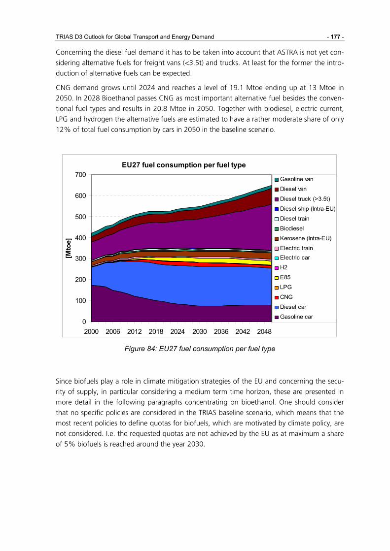
TRIAS D3 Outlook for Global Transport and Energy Demand - 177 -
Concerning the diesel fuel demand it has to be taken into account that ASTRA is not yet con-
sidering alternative fuels for freight vans (<3.5t) and trucks. At least for the former the intro-
duction of alternative fuels can be expected.
CNG demand grows until 2024 and reaches a level of 19.1 Mtoe ending up at 13 Mtoe in
2050. In 2028 Bioethanol passes CNG as most important alternative fuel besides the conven-
tional fuel types and results in 20.8 Mtoe in 2050. Together with biodiesel, electric current,
LPG and hydrogen the alternative fuels are estimated to have a rather moderate share of only
12% of total fuel consumption by cars in 2050 in the baseline scenario.
EU27 fuel consumption per fuel type
0
100
200
300
400
500
600
700
2000 2006 2012 2018 2024 2030 2036 2042 2048
[Mto
e]
Gasoline van
Diesel van
Diesel truck (>3.5t)
Diesel ship (Intra-EU)
Diesel train
Biodiesel
Kerosene (Intra-EU)
Electric trainElectric car
H2
E85
LPG
CNG
Diesel car
Gasoline car
Figure 84: EU27 fuel consumption per fuel type
Since biofuels play a role in climate mitigation strategies of the EU and concerning the secu-
rity of supply, in particular considering a medium term time horizon, these are presented in
more detail in the following paragraphs concentrating on bioethanol. One should consider
that no specific policies are considered in the TRIAS baseline scenario, which means that the
most recent policies to define quotas for biofuels, which are motivated by climate policy, are
not considered. I.e. the requested quotas are not achieved by the EU as at maximum a share
of 5% biofuels is reached around the year 2030.
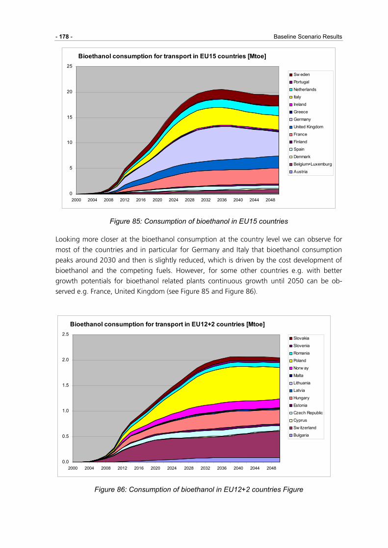
- 178 - Baseline Scenario Results
Bioethanol consumption for transport in EU15 countries [Mtoe]
0
5
10
15
20
25
2000 2004 2008 2012 2016 2020 2024 2028 2032 2036 2040 2044 2048
Sw eden
Portugal
Netherlands
Italy
Ireland
Greece
Germany
United Kingdom
France
Finland
Spain
Denmark
Belgium+Luxemburg
Austria
Figure 85: Consumption of bioethanol in EU15 countries
Looking more closer at the bioethanol consumption at the country level we can observe for
most of the countries and in particular for Germany and Italy that bioethanol consumption
peaks around 2030 and then is slightly reduced, which is driven by the cost development of
bioethanol and the competing fuels. However, for some other countries e.g. with better
growth potentials for bioethanol related plants continuous growth until 2050 can be ob-
served e.g. France, United Kingdom (see Figure 85 and Figure 86).
Bioethanol consumption for transport in EU12+2 countries [Mtoe]
0.0
0.5
1.0
1.5
2.0
2.5
2000 2004 2008 2012 2016 2020 2024 2028 2032 2036 2040 2044 2048
Slovakia
Slovenia
Romania
Poland
Norw ay
Malta
Lithuania
Latvia
Hungary
Estonia
Czech Republic
Cyprus
Sw itzerland
Bulgaria
Figure 86: Consumption of bioethanol in EU12+2 countries Figure
TRIAS D3 Outlook for Global Transport and Energy Demand - 179 -
5.6 Environment
The following chapter describes the observed environmental trends in the TRIAS baseline. The
presented figures and graphs were extracted from ASTRA showing national emission trends,
from POLES-TRIAS demonstrating upstream emissions from electricity and from Regio-
SUSTAIN analysing regional immissions for two case study regions.
ASTRA Emissions
The displayed graphs in the following chapter summarise the observed trends for air emis-
sions and fuel consumption in EU27 in the TRIAS baseline scenario. Figure 87 opposes esti-
mated transport performance and air emission trends for the period from 2000 to 2050. The
figure highlights passenger transport trends in terms of passenger-km and freight transport
trends in terms of ton-km. As described in the chapter on transport results, passenger-km are
growing only slightly influenced by stagnating or even declining population in EU27 by
+38.9% until 2030 and rather moderate +51.3% until 2050. As opposed this freight trans-
port is impacted strongly by high foreign trade and national production value growth rates.
Ton-km are assessed to double until 2030 and even more than triple until 2050 in EU27.
Against the background of increasing passenger and especially freight transport the illus-
trated CO2 emission projections show that business-as-usual measures implemented in the
baseline scenario Euro 6 are by far not sufficient concerning the greenhouse gas emission
reduction targets. Carbon dioxide reduction targets like the agreement of EU member states
on overall –30% reduction until 2020 compared with 1990 require stronger incentives for
the transport sector. The baseline scenario simulation considering the changing technological
improvements of vehicle fleets in EU27 illustrate positive growth of CO2 emissions from
transport until 2050. Due to the baseline simulation CO2 emissions are expected to increase
by +25.3% until 2030, +35.5% until 2040 and +48.6% until 2050 compared with the base
year 2000. Technological improvements cannot balance increasing transport performance
and growing motorisation.
In contrast NOx emission projections demonstrate the impacts of significant technological
improvements. ASTRA assesses NOx emission reductions by –54.8% in 2030, -53.2% in 2040
and –50.2% in 2050. In the last two decades NOx emissions stagnate in EU27 mainly due to
growing importance and share of freight transport. Besides CO2 and NOx ASTRA considers
also CO and VOC emissions caused by the transport sector. The baseline projections estimate
–24.3% decline of CO emissions until 2030 and –7.6% reduction until 2050 compared with
2000. VOC emissions increase until 2030 by +11.2% and even +32.6% until 2050.

- 180 - Baseline Scenario Results
EU27 development air emissions from transport
0
25
50
75
100
125
150175
200
225
250
275
300
325
350
2000
2004
2008
2012
2016
2020
2024
2028
2032
2036
2040
2044
2048
[Inde
x B
ase
Year
200
0 =
100]
COCO2NOxVOCtkmpkm
Figure 87: EU27 air emission trends versus transport performance
Figure 88 allows a more detailed analysis of CO2 emissions in the baseline scenario. The fig-
ure differentiates CO2 emission trends per origin respective transport mode. Having the sig-
nificant freight transport growth in mind the high emission growth rate for CO2 produced by
freight transport is not astonishing. Freight transport CO2 emissions grow by about +1.9%
yearly and until 2050 by +153.7% compared with the base year. As opposed passenger
transport CO2 emissions increase only slightly by +12.6% until 2016 and decline afterwards
reaching with a small plus of + 2.9% nearly the same level as in base year. Strongest growing
freight transport mode in terms of CO2 emissions is with distance heavy duty vehicle trans-
port increasing nearly by +249% until 2050. Compared with the emission trends observed
for heavy duty vehicles CO2 emissions from light duty vehicles reflect a slight saturation of
EU27 markets with LDVs and a less strong increase as for HDVs.
Regarding CO2 emissions from passenger transport the expanding modal share of air trans-
port is of growing importance and results in +45.6% growth until 2050. ASTRA assesses
stagnating or even reducing CO2 emissions from all other passenger transport modes: car,
bus and passenger train. Passenger car emissions stay on nearly the same level as in the year
2000 while emissions from bus and passenger train transport are estimated to be reduced by
–37.3% respective -18% until 2050.

TRIAS D3 Outlook for Global Transport and Energy Demand - 181 -
EU27 CO2 emission trends
5075
100
125
150175200
225250
275300325
350
2000
2004
2008
2012
2016
2020
2024
2028
2032
2036
2040
2044
2048
[Inde
x B
ase
Year
200
0 =
100] CO2 passenger
CO2 freightCO2 carCO2 busCO2 ptrainCO2 airCO2 hdvCO2 ldvCO2 ftrainCO2 ship
Figure 88: EU27 CO2 emission trends per mode
Figure 89 substantiates the relative emission trends for CO2 demonstrated in the previous
figure. The depicted absolute emission values clarify the importance of growing heavy duty
vehicle transport for strategies facing the problem of global climate change. Comparing the
situation in the year 2000 and in 2050 there is a significant trend visible: in the base year
heavy duty freight transport produced about 17.6% of all transport CO2 emissions while pas-
senger car transport was the main polluter with a share of 54.7%. In 2050 cars will be re-
sponsible for 36.2% of all transport CO2 emissions while heavy duty transport reaches even a
share of 39.8%.

- 182 - Baseline Scenario Results
EU27 CO2 emissions per mode
0
200
400
600
800
1000
1200
1400
1600
1800
2000
2004
2008
2012
2016
2020
2024
2028
2032
2036
2040
2044
2048
[Mio
t C
O2]
CO2 shipCO2 ftrainCO2 ldvCO2 hdvCO2 airCO2 ptrainCO2 busCO2 car
Figure 89: EU27 absolute CO2 emissions per mode
The following figures demonstrate the development of NOx emissions caused by transport
activities in the baseline scenario. In the context of climate change debate the pollutant NOx
took a back seat compared with CO2. Regarding the dangers caused by NOx emissions like
acidification, health problems, increasing smog and ozone appearance, the simulated trends
are not subordinate and have to be analysed critically as well.
Figure 90 presents NOx emission indices based on the year 2000 showing the prospective
emission trends per transport mode respective transport sector. Results of the baseline sce-
nario confirm that NOx emissions caused by passenger transport can be reduced significantly
by –62.1% until 2030 and -58.8% until 2050. The strong decrease of NOx emissions is
mainly caused by car technology improvements like the introduction of three-way catalytic
converters or NOx storage catalysts and the disappearance of cars with old technologies.
ASTRA projects a slower substitution of old NOx intensive by modern NOx reducing technolo-
gies for freight transport. This is mainly influenced by the high share of diesel heavy and light
duty vehicles. Most modern gasoline cars or light duty vehicles are equipped with catalytic
converters while still not all diesel cars or trucks are equipped with NOx storage catalysts. De-
spite the slower technological diffusion NOx emissions caused by freight transport decrease
by –65% until 2030 and –56.6% until 2050. In contrast to CO2 emission trends NOx emis-
sions increase most significantly by passenger air transport with +53.6% until 2030 and
+81.6% until 2050 followed by ship (inland waterway) with +28.5% until 2030 and +52.6%
until 2050. Passenger car and light duty vehicle motor technology enable a decline of NOx
emissions by –91.8% respective –87.9% until 2030 and –92.5% respective –80.8% until
2050.
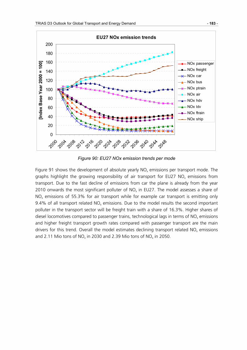
TRIAS D3 Outlook for Global Transport and Energy Demand - 183 -
EU27 NOx emission trends
0
20
40
60
80
100
120
140
160
180
200
2000
2004
2008
2012
2016
2020
2024
2028
2032
2036
2040
2044
2048
[Inde
x B
ase
Year
200
0 =
100] NOx passenger
NOx freightNOx carNOx busNOx ptrainNOx airNOx hdvNOx ldvNOx ftrainNOx ship
Figure 90: EU27 NOx emission trends per mode
Figure 91 shows the development of absolute yearly NOx emissions per transport mode. The
graphs highlight the growing responsibility of air transport for EU27 NOx emissions from
transport. Due to the fast decline of emissions from car the plane is already from the year
2010 onwards the most significant polluter of NOx in EU27. The model assesses a share of
NOx emissions of 55.3% for air transport while for example car transport is emitting only
9.4% of all transport related NOx emissions. Due to the model results the second important
polluter in the transport sector will be freight train with a share of 16.3%. Higher shares of
diesel locomotives compared to passenger trains, technological lags in terms of NOx emissions
and higher freight transport growth rates compared with passenger transport are the main
drivers for this trend. Overall the model estimates declining transport related NOx emissions
and 2.11 Mio tons of NOx in 2030 and 2.39 Mio tons of NOx in 2050.

- 184 - Baseline Scenario Results
EU27 NOx emissions per mode
00.5
11.5
22.5
33.5
44.5
55.5
6
2000
2004
2008
2012
2016
2020
2024
2028
2032
2036
2040
2044
2048
[Mio
t NO
x]
NOx shipNOx ftrainNOx ldvNOx hdvNOx airNOx ptrainNOx busNOx car
Figure 91: EU27 absolute NOx emissions per mode
POLES-TRIAS Emissions
POLES-TRIAS Upstream Emissions Electricity
In EU-27 countries total carbon dioxide emissions from electricity production increases con-
stantly by an average of 1.2% from 2006 until 2041 when it reaches around 2033 MtCO2.
Beyond 2041 this total emission can be expected to undergo slight decrease. In term of share
of the total CO2 emission from electricity production in the world, EU-27 is estimated to con-
tribute around 15% in 2006 and 12% in 2050.
Figure 92 below shows how electricity production by solid fuel (coal) has the lion share of the
total CO2 emission between 2001 and 2050. This share oscillates between 65 to 75% of the
total emission during the period. The share of CO2 emission from electricity production by
natural gas increases steadily from 18% in 2006 to 31% in 2050 while the share of CO2
emission from production by liquid (oil) fuel remains the lowest with 6.1% in 2006 decreas-
ing to 2.8% in 2050.

TRIAS D3 Outlook for Global Transport and Energy Demand - 185 -
0
500
1000
1500
2000
2500
2001
2004
2007
2010
2013
2016
2019
2022
2025
2028
2031
2034
2037
2040
2043
2046
2049
MtC
O2 Solid
LiquidGas
Figure 92: Share of CO2 emissions from electricity production in EU-27 countries
Regio-SUSTAIN: Analysis of regional immissions
The Regio-SUSTAIN model has been developed for the analysis of regional impacts. During
the TRIAS project it has been expanded and updated for the objectives of the project. The
following chapter describes the results of Regio-SUSTAIN for the Reference scenario in 2000.
First, the two investigations areas are defined. Second, the major roads of the areas and the
considered substances are described. Finally, the results for the Reference scenario 2000 are
displayed and explained.
Areas under consideration
Regio-SUSTAIN has been developed for regional analyses. It is based on a huge database,
which could not be applied for the whole area of Europe. Regio-SUSTAIN provides regional
and local indicators depending on transport activity and energy use. The consortium decided
to analyse the development of local pollution in two case-study regions, namely the Ruhr
area and the South of Spain. Boundaries for the two regions are based on the Nomenclature
of Territorial Units of Statistics (NUTS). The NUTS III classification has been applied for the
TRIAS project. Table 44 displays the regions under consideration.

- 186 - Baseline Scenario Results
Table 44: NUTS III regions under consideration for the regional environmental assess-ment
Ruhr area South of Spain
NUTS III classifica-
tion
Name of region NUTS III classifica-
tion
Name of re-
gion
DEA11 Düsseldorf ES613 Cordoba
DEA12 Duisburg ES615 Huelva
DEA13 Essen ES618 Sevilla
DEA16 Mühlheim
DEA17 Oberhausen
DEA1C Mettmann
DEA31 Bottrop
DEA32 Gelsenkirchen
DEA51 Bochum
DEA52 Dortmund
DEA55 Herne
DEA56 Ennepe-Ruhr-
Kreis
DEA5C Unna
The analysed Ruhr area has a West-East elongation of approx 80 km and a North-South
elongation of approx 50 km. The region has been chosen for analysis because of its great
population density and the major road axis which passes the area, namely the German mo-
torways A1, A2 and A3. Furthermore, the Ruhr area consists of a number of large industrial
cities, which have been dependent on coal mining and steel production. Nowadays, steel
production still plays an important role in the area but the introduction of engineering indus-
tries as well as the service sector shows the structural change of the area. For the assessment
of emissions from stationary facilities (e.g. steel industry, etc.) and its future development the
Ruhr area serves as a good example. Figure 93 maps the area under consideration.

TRIAS D3 Outlook for Global Transport and Energy Demand - 187 -
Figure 93: Ruhr area (Germany) as assessed in the TRIAS project (GoogleMaps, 2007)
The second area under consideration for the regional assessment of emissions is Andalusia in
Spain. Andalusia has a total population of around 8 million and covers an area of approx
87,000 km² (Junta de Andalucia, 2007). The cities of Seville, Granada, Cadiz and Malaga
belong to the autonomous community of Spain. The economy of Andalusia is based on the
three pillars: industrial production (mining, chemistry and shipbuilding), agriculture and ser-
vice sector. Especially the development of the industrial sector has been of major concern for
the TRIAS project. Emissions from stationary facilities coming from the industry as well as
transport exhaust emissions are considered in the assessment. Figure 94 shows the area of
Andalusia, which has been analysed for the TRIAS regional environmental assessment.
Figure 94: Andalusia (Spain) as assessed in the TRIAS project (GoogleMaps, 2007)

- 188 - Baseline Scenario Results
Major roads and emission facilities
The location of stationary facilities has been provided by the Poles model for both investiga-
tion areas. Poles considers the five industry sectors which have been implemented into Regio-
SUSTAIN:
• Chemical industry (CHI),
• Service sector (SER),
• Steel industry (STI),
• Non metallic mineral industry (NMM) and
• Other industries (OIN).
For the objective of analysing emission and immission concentrations the major polluting
sectors are chemical, steel and non-metallic mineral. In the Ruhr area a concentration of
chemical and steel industry can be found whereas in Andalusia steel and non-metallic mineral
companies are mainly represented. In total over 70 stationary facilities are considered for the
TRIAS project.
The major roads for both investigation areas are national motorways and national highways.
VACLAV has provided data for the trunk roads, including location of the links and their traffic
loads. In the Ruhr area a large number of national motorways exist. The area is densely popu-
lated and can be classified as urban. The cities are connected by highways as well as motor-
ways. Three of the most congested German motorways are located in this area, namely the
motorway A1 (E372), A2 (E343) and A3 (E354). Other motorways that have been considered
are A40 (E34), A42, A43, A 44, A45 (E31), A46 (E37), A52 and A59. Furthermore, the largest
federal highways are included in the immission calculation.
With a population density of around 90 persons per sqkm, Andalusia can be classified as a
rural region with some major urban settlements. These cities are linked by motorways, which
have been introduced into the model. The main motorways of Andalusia are A4 (E5), AP4
(E5) and A49 (E1). Also smaller motorways and highways, such as A45, A66, A92, N420 and
A432 have been considered for the TRIAS project.
Analysed Substances
Regio-SUSTAIN analyses regional impacts of the transport and energy sector. Therefore, sub-
stances have been chosen which have local impacts on the environment. The focus of the
analysis has been placed on Particulate Matter (PM) and Nitrogen Oxides (NOx).
2 The European E-network consists of roads which cross national boarders and which have been
defined as important roads for Europe by the United Nations Economic Commission of Europe. The E37 is located in Germany. It is a North-South axis starting in Delmenhorst (Fed-eral state of Lower Saxony) and terminates in Cologne.
3 E34: Antwerp (Belgium) – Venlo (The Netherlands) – Dortmund (Germany) – Bad Oeynhausen (Germany)
4 E35: Amsterdam (The Netherlands) – Düsseldorf (Germany) – Karlsruhe (Germany) – Basel (Switzerland) – Milan (Italy) –Rome (Italy)

TRIAS D3 Outlook for Global Transport and Energy Demand - 189 -
Particles are one of the most influential emission factors on a regional scale. Breathing fine
particles have substantial adverse impacts on human health. Inhaling high concentrations
over a long period may lead to asthma, lung cancer, cardiovascular issues and premature
deaths. Therefore, legislation of the European Commission is aimed at reducing the concen-
tration of particles significantly over the next decade.
Nitrogen oxides are associated with reduced lung functions, which lead to irritations and
damage of the respiratory organ. Especially short-term exposure of high concentrations at a
local and regional level leads to high impacts on human health. These characteristics of NOx
have been the reason to include the substance into the evaluation sample.
Results for the Reference Scenario 2000
The baseline scenario as defined in the first part of the TRIAS project displays the situation in
the year 2000. No scenarios are applied and the situation as it has happened is calculated.
The results of the regional immission calculation for the transport sector are displayed in
Figure 95 for nitrogen oxides and in Figure 96 for particles. The major motorways with the
highest transport loads in the Ruhr area can be ascertained from the figures, namely the A3
(North-South axis in the western parts of the region) and the A46, which passes over to the
A1 (West-East axis starting in the south of the region). Both axis are mostly used for long
distance traffic, especially HGVs coming from the Dutch ports with destinations in the South
or East of Germany respectively Europe. The highest concentrations of NOx and PM are
found in east direction of the analysed motorway. The reason is that a constant average wind
field has been applied to the model that has been calibrated on long-term time series for the
Ruhr area. The assumption is a constant wind field of 225° (South-East direction) with an
average speed of 2.5 m/s. Expert interviews have shown that the assumptions are acceptable.
The interpretation of the figures should be focused on changes over time and changes with
different scenarios. Absolute values of the figures are indicators for the situation in the region
but the focus of TRIAS is on long-distance transport and energy pollutants only. Therefore,
inner city traffic and pollutants from households go behind the objectives of the project but
should be considered when analysing absolute values.

- 190 - Baseline Scenario Results
Figure 95: NOx immissions in the Ruhr area (Baseline scenario for 2000)
Figure 96: PM immissions in the Ruhr area (Baseline scenario for 2000)
The situation for Andalusia is slightly different as for the Ruhr area. Instead of a large number
of motorways crossing the area only few major roads are available. The most important roads
in Andalusia are the A49 (E1) and A4 (E5), which cross the region from West to East. This can
also be observed when analysing the immission maps, especially the NOx map. The highest
concentration for NOx can be found in the eastern parts of the region where the landscape
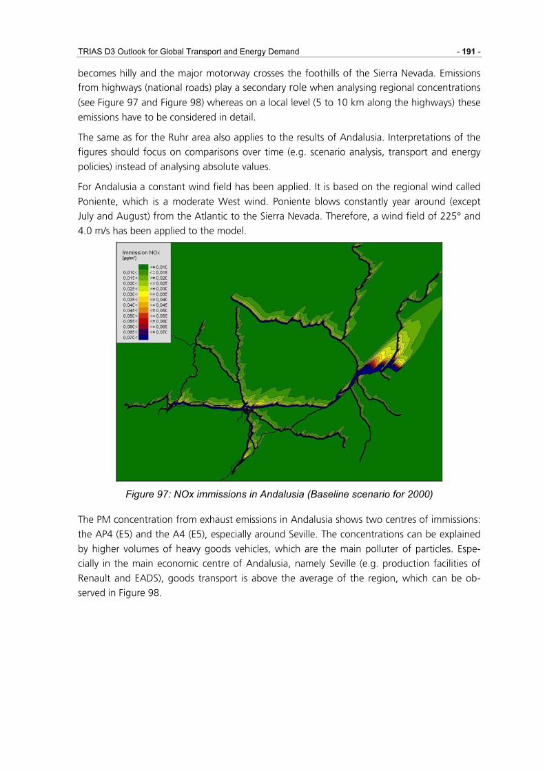
TRIAS D3 Outlook for Global Transport and Energy Demand - 191 -
becomes hilly and the major motorway crosses the foothills of the Sierra Nevada. Emissions from highways (national roads) play a secondary role when analysing regional concentrations
(see Figure 97 and Figure 98) whereas on a local level (5 to 10 km along the highways) these
emissions have to be considered in detail.
The same as for the Ruhr area also applies to the results of Andalusia. Interpretations of the
figures should focus on comparisons over time (e.g. scenario analysis, transport and energy
policies) instead of analysing absolute values.
For Andalusia a constant wind field has been applied. It is based on the regional wind called
Poniente, which is a moderate West wind. Poniente blows constantly year around (except
July and August) from the Atlantic to the Sierra Nevada. Therefore, a wind field of 225° and
4.0 m/s has been applied to the model.
Figure 97: NOx immissions in Andalusia (Baseline scenario for 2000)
The PM concentration from exhaust emissions in Andalusia shows two centres of immissions:
the AP4 (E5) and the A4 (E5), especially around Seville. The concentrations can be explained
by higher volumes of heavy goods vehicles, which are the main polluter of particles. Espe-
cially in the main economic centre of Andalusia, namely Seville (e.g. production facilities of
Renault and EADS), goods transport is above the average of the region, which can be ob-
served in Figure 98.

- 192 - Baseline Scenario Results
Figure 98: PM immissions in Andalusia (Baseline scenario for 2000)

TRIAS D3 Outlook for Global Transport and Energy Demand - 193 -
6 Conclusions and Outlook
In the TRIAS project a "Sustainability Impact Assessment of Strategies Integrating Transport,
Technology and Energy Scenarios" is performed. Considering emerging constraints of fossil
energy, prospective transport performance trends, potential technology trends for alternative
fuels of transport and possible policies to foster fuel switch of transport the TRIAS project
assesses potential sustainability implications. This report first concentrates mainly on the de-
scription of the tools applied for assessing the potential impacts, the development and revi-
sion of these tools, their linkage and assumptions. Second the TRIAS baseline scenario is pre-
sented.
Modelling and tool development
The following five models are improved and linked in TRIAS:
• POLES and BIOFUEL display world-wide energy demand and supply,
• ASTRA simulates national economies, sectoral foreign trade and transport on an ag-
gregate level,
• VACLAV models detailed transport network impacts on NUTSIII level, and
• Regio-SUSTAIN identifies local environmental impacts for two selected European re-
gions.
Linking ASTRA with POLES and BIOFUEL enables to exchange endogenously calculated en-
ergy prices and energy demand from transport within a closed feedback loop that connects
the world energy system with the European transport system. Integrating the transport net-
work model VACLAV in this modelling framework represents another important value-added
of TRIAS. Congestion effects and existing infrastructure can be considered with VACLAV and
can be combined with ASTRA simulating all socio-economic indicators relevant for the gen-
eration of transport demand, which in turn closes the feedback loop between the transport
system and the economic system. Additionally, TRIAS enables a detailed overview on scenario
implications for specific case studies by integrating the regional immission model Regio-
SUSTAIN into the modelling suite.
Regarding technological scenarios focussed on transport the TRIAS modelling framework
demonstrated a good performance with the integration of alternative fuel technologies like
hydrogen and biofuels. These technologies are represented with their implications on both
side i.e. in the energy system and the transport system.
Furthermore, TRIAS developed two new concepts for integrated modelling across discipline:
first, a tool that allows distributed modelling on System Dynamics Models of the ASTRA type,
the ASTRA-Merger, is developed. This enables the implementation of the split-and-merge
concept for ASTRA, which increases enormously the efficiency of conjoint model develop-
ment by working in different teams on separate small-size files that are version-controlled by
a repository. Second, TRIAS proved that the use of such a repository for soft-linking between
models like POLES and ASTRA enables to create model linkages with a high number of itera-
tions of data between the models in a fast and traceable manner.
- 194 - Conclusions and Outlook
TRIAS baseline scenario
The Baseline Scenario of TRIAS is constructed in general as a business-as-usual scenario as-
suming no major disruptions for the next 45 years, i.e. no strong policy changes are consid-
ered. This does not mean that we would not expect them, as for instance in the case of cli-
mate policy we would expect a rather more ambitious approach in the next decades then up
to now. But it means that the baseline scenario is not including such major changes of the
systems under analysis.
Hence, the TRIAS baseline scenario expects continuous economic growth, of course with dif-
ferent speeds by country and by world region, moderate technological improvements in
terms of energy efficiency and in terms of the emergence and diffusion of new technologies
in the energy and transport system as well as continued globalisation accompanied with
strong growth of World and European trade. The main element where a change of develop-
ment in the future compared with the past is expected by the models concerns the demog-
raphy. European population will grow slightly until about 2020 and then starts to decline.
The structure of the population will even change significantly with an increase of +50% of
persons above 65 years of age, and a corresponding decrease of younger age classes. On
country level population trends can be quite different e.g. declining earlier like in most new
member states or continuing to grow like in Sweden.
One of the main conclusions of the TRIAS baseline scenario is that under such a baseline sce-
nario transport energy demand and also CO2 emissions are still increasing in the next decades
until 2050. Nearly 50% growth of CO2 emissions compared with the year 2000 indicates that
the EU27 is miles away from climate protection targets. Passenger and freight transport per-
formance are projected to increase further until 2050 by +50% respective more than
+200%. Transport volumes grow at a lower pace, which indicates that part of transport
growth is still driven by longer travel distances. This means, energy efficiency improvements
in transport technology are too moderate too compensate the transport demand growth.
Regarding the technological composition of prospective EU27 vehicle fleets the diesel tech-
nology will have the highest share followed by gasoline. Since the baseline scenario does not
consider subsidies for hydrogen this technology will not diffuse into EU27 vehicle markets.
Instead, the ASTRA baseline scenario simulation projects that in the short to medium term
technologies like CNG and hybrid will be alternatives to today’s petroleum based internal
combustion engines (ICE), while in the medium term bioethanol becomes more important.
Interestingly, in the long-term gasoline blended with bioethanol and burned in new highly
fuel efficient combustion engines recaptures part of the lost market share.
Regarding these trends and the fact that there is no revolutionary technological change ex-
pected in the baseline scenario, more radical technological shifts from fossil to alternative
fuels and behavioural changes of individual mobility must be fostered to cope with scarcity of
fossil fuels and with the need for ambitious climate protection. Potential scenarios that give
some answers on how to reduce fossil fuel dependency of transport and contribute to cli-
mate protection targets in EU27 are presented in the TRIAS D4 report.

TRIAS D3 Outlook for Global Transport and Energy Demand - 195 -
7 References
ACI – Automobile Club Italia (2006), Costi chilometrici di esercizio di alcuni tipi di autovettu-
re, autofurgoni e motoveicoli, Automobile Club d’Italia, Roma (Italy).
Amann, M., Cofala, J., Heyes, C., Klimont, Z., Mechler, R., Posch, M., Schöpp, W., (2004)
RAINS Review 2004, The RAINS model: Documentation of the model approach pre-
pared for the RAINS peer review 2004, International Institute for Applied Systems
Analysis
Aral (2005): "Aral Studie – Trends beim Autokauf 2005". Aral Press, Bochum.
Autobus (2005), No. 15, pag. 103-107, VTE Edizioni, Cassano d’Adda, Milano (Italy).
Banse M (2000): "Social Accounting Matrices for 13 European countries for the IASON pro-
ject". Download at: http://www.regroningen.nl/irios/iriostables.htm.
Boitani A., Cambini C. (2001), La riforma del trasporto pubblico locale in Italia: problemi e
prospettive, HERMES Working Paper No.4, Moncalieri, Turin (Italy).
Bossel H (1994): "Modellbildung und Simulation – Konzepte, Verfahren und Modelle zum
Verhalten dynamischer Systeme", 2nd edition, Vieweg, Brunswick.
Cambini C., Galleano F. (2005), Le gare per l’affidamento del servizio di trasporto pubblico
locale in Italia. II° Rapporto, HERMES, Moncalieri, Turin (Italy).
Cambini C., (2003), La situazione delle gare per l’affidamento del servizio di trasporto urbano
in Italia, HERMES, Moncalieri, Turin (Italy).
Cicini P., Macchia G, Giuseppetti A. (2005), “Progetti ferroviari: dall’analisi finanziaria
all’analisi economica”, Argomenti, Year 3, No. 5, 6-37, RFI, Rome (Italy).
Cofala, J., Syri, S., (1998) Nitrogen Oxides Emissions, Abatement Technologies and Related
Costs for Europe in the RAINS Model Database, IIASA Interim Report, IR-98-88, Interna-
tional Institute for Applied Systems Analysis
CSO - Central Statistical Office (1992): "Input-Output Balance for the United Kingdom:
1989", London.
CSST - Centro Studi sui Sistemi di Trasporto (2005), Indagine conoscitiva sui costi e sulla fisca-
lità sopportati dalle imprese italiane di autotrasporto di cose per conto di terzi, raffron-
tati con quelli di analoghe imprese appartenenti ai paesi dell’Unione Europea alla data
del 1° gennaio 2005, Ministero dei Trasporti e della Navigazione, Comitato Centrale
per l’Albo degli Autotrasportatori di cose per conto di terzi, Roma (Italy).
De Ceuster G. et al (2005), ASSESS Final Report, DG TREN, European Commission.
Dell’Aringa C. (2004), Tariffe e ricavi da traffico nelle aziende del trasporto pubblico locale:
1996 – 2004, HERMES, Moncalieri, Turin (Italy).
Earchimede (2004), Benchmark europeo e linee guida per lo sviluppo del TPL italiano, presen-
ted at conference La resa dei conti, Roma (Italy).
- 196 - References
European Commission (2006): Annexes to the report from the Commission to the Council on
the review of the energy crops scheme. SEC(2006) 1167.
EC (2003): Directive 2003/96/EC of 27 October 2003 restructuring the Community frame-
work for the taxation of energy products and electricity.
EC (2007): Limiting Global Climate Change to 2 degrees Celsius. The way ahead for 2020
and beyond. COM (2007)2.
EUROSTAT (1998): "Harmonised Input-Output-Tables for the EU15 Countries", EXCEL-Files
provided by EUROSTAT datashop, Luxemburg.
EUROSTAT (2002): "Regions: Statistical Yearbook 2002", CD-ROM, Luxembourg.
Gühnemann A (2000): “Methods for Strategic Environmental Assessment of Transport Infra-
structure Plans”, Dissertation thesis at IWW, Nomos Verlag, Baden-Baden.
Heckscher E (1919): "The Effect of Foreign Trade on the Distribution of Income," in: Ekono-
misk Tidskrift, pp 497-512.
INFRAS (2000), Variabilisation and differentiation strategies in road taxation, ECMT.
IPCC (2001) Third Assessment Report
IPSOS (2004), Indagine conoscitiva su 2.000 imprese che esercitano l’autotrasporto di cose
per conto di terzi, Ministero dei Trasporti e della Navigazione, Comitato Centrale per
l’Albo degli Autotrasportatori di cose per conto di terzi, Roma (Italy).
IWW, IFEU, Kessel+Partner, Planungsgruppe Ökologie, PTV Consult (1998): “Entwicklung
eines Verfahrens zur Aufstellung umweltorientierter Fernverkehrskonzepte als Beitrag
zur Bundesverkehrswegeplanung”, Report on behalf of the German Federal Environ-
mental Agency, Erich-Schmidt Verlag, Berlin.
IWW, TRT, ME&P, CEBR (2000): "ASTRA Methodology", Deliverable D4 of the ASTRA (As-
sessment of Transport Strategies) project funded by the European Commission 4th RTD
framework, Karlsruhe.
Janssen, A.; Lienin, S.F.; Gassmann, F.; Wokaun, A. (2004): "Model aided policy development
for the market penetration of natural gas vehicles in Switzerland". Transportation Re-
search Part A, Elsevier.
JRC, EUCAR, CONCAWE (2006): Well-to-Wheels analysis of future automotive fuels and
powertrains in the European context, WELL-to-WHEELS report, Version 2b, May 2006.
Leetmaa P. (2006), Relative price levels for new passenger cars in Europe for 2004, Statistics
in focus, Economy and Finance, No. 3/2006, EUROSTAT
Kavalov, B., Jensen, P., Papageorgiou, Schwensen, C., Olsson, J.P. (2003): Biofuel Pro-duction
Potential of EU Candidate Countries, Final Report, EUR 20835 EN, JRC-IPTS, September
2003.
Klimont, Z., Cofala, J., Bertok, I., Amann, M., Heyes, C., Gyarfas, F., (2002), Modeling Par-
ticulate Emissions in Europe. A Framework to Estimate Reduction Potential and Control Cost, International Institute for Applied Systems Analysis

TRIAS D3 Outlook for Global Transport and Energy Demand - 197 -
Martens M. et al, (2005), Modelling scenarios and assumptions, Annex V of ASSESS Final
Report, DG TREN, European Commission.
McCormick K., Peck, P., Kaberger, T. (2006): Breaking dependence on oil in Sweden: explor-
ing the implications for biofuels, Energy for Sustainable Development, June 2006.
ME&P (2000): "SCENES European Transport Forecasting Model and Appended Module:
Technical Description", Deliverable D4 of SCENES (Modelling and methodology for
analysing the interrelationship between external developments and European transport)
project funded by the European Commission 4th RTD framework, Cambridge.
OECD/EEA (2006), Database on instruments used for environmental policy and natural re-
sources management, http://www2.oecd.org/ecoinst/queries/index.htm (last visit:
29/06/06).
Ortuzar JD, Willumsen LG (1998): "Modelling Transport", second edn, JohnWiley and Sons,
New York.
Prenzel, T. (2006): "Die Werbung deutscher Automobilhersteller". Published by Bund für
Umwelt und Naturschutz Deutschland e.V. (BUND), Berlin.
RFI (2005), Prospetto Informativo della Rete, RFI, Rome (Italy).
SCENES (2000): Web-Database of the SCENES project (Modelling and methodology for ana-
lysing the interrelationship between external developments and European transport)
funded by the European Commission 4th RTD framework, http://www.iww.uni-
karlsruhe.de/SCENES/, 22.01.2002.
Schade B, Rothengatter W, Schade W (2002): "Strategien, Maßnahmen und ökonomische
Bewertung einer dauerhaft umweltgerechten Verkehrsentwicklung" (Strategies, In-
struments and Economic Assessment of Environmentally Sustainable Transport (EST)).
Final report on behalf of the German Federal Environmental Agency, Erich-Schmidt-
Verlag, Berlin.
Schade W (2005): "Strategic Sustainability Analysis: Concept and application for the assess-
ment of European Transport Policy". Dissertation thesis at IWW, Nomos Verlag, Baden-
Baden.
Schöpp, W., Amann, M., Cofala, J., Heyes, C. and Klimont, Z. (1999) Integrated Assessment
of European Air Pollution Emission Control Strategies. Environmental Modeling and
Software 14(1).
StaBA – Statistisches Bundesamt (1997): "Volkswirtschaftliche Gesamtrechungen: Reihe 2
Input-Output-Tabellen 1993", Metzler-Poeschel, Stuttgart.
Sterman JD (2000): "Systems Thinking and Modeling for a Complex World", Irwin McGraw-
Hill, Boston.
The AA Motoring Trust (2006), The cost of motoring – 2006, The AA Motoring Trust (Great
Britain)
TIS (2002), Study on vehicle taxation in the member states of the European Union, European
Commission.

- 198 - References
VIEWLS (2005): Environmental and economic performance of biofuels, project report for the
project VIEWLS (Clear Views on Clean Fuels), April 2005.
Wiesenthal T.; P. Christidis, B. Schade, L. Pelkmans (forthcoming): Scenario-based as-
sessment of biofuel policies in the EU. PREMIA WP6 report, forthcoming.
Related Documents