arXiv:0903.2421v2 [math.PR] 28 Feb 2010 Outliers in INAR(1) models M ´ aty ´ as Barczy ∗,⋄ , M ´ arton Isp ´ any ∗ , Gyula Pap ∗∗ , Manuel Scotto ∗∗∗ and Maria Eduarda Silva ∗∗∗∗ * University of Debrecen, Faculty of Informatics, Pf. 12, H–4010 Debrecen, Hungary; ** University of Szeged, Bolyai Institute, H-6720 Szeged, Aradi v´ ertan´ uk tere 1, Hungary; *** Universidade de Aveiro, Departamento de Matem´ atica, CampusUniversit´ario deSantiago, 3810-193 Aveiro, Portugal; **** Universidade do Porto, Faculdade de Economia, Rua Dr. Roberto Frias s/n, 4200 464 Porto, Portugal. e–mails: [email protected] (M. Barczy), [email protected] (M. Isp´ any), [email protected] (G. Pap), [email protected] (M. Scotto), [email protected] (M. E. Silva). ⋄ Corresponding author. Abstract In this paper the integer-valued autoregressive model of order one, contaminated with additive or innovational outliers is studied in some detail. Moreover, parameter estimation is also addressed. Supposing that the time points of the outliers are known but their sizes are unknown, we prove that the Conditional Least Squares (CLS) estimators of the offspring and innovation means are strongly consistent. In contrast, however, the CLS estimators of the outliers’ sizes are not strongly consistent, although they converge to a random limit with probability 1. This random limit depends on the values of the process at the outliers’ time points and on the values at the preceding time points and in case of additive outliers also on the values at the following time points. We also prove that the joint CLS estimator of the offspring and innovation means is asymptotically normal. Conditionally on the above described values of the process, the joint CLS estimator of the sizes of the outliers is also asymptotically normal. 2000 Mathematics Subject Classifications : 60J80, 62F12. Key words and phrases : integer-valued autoregressive models, additive and innovational outliers, conditional least squares estimators, strong consistency, conditional asymptotic normality. The authors have been supported by the Hungarian Portuguese Intergovernmental S & T Cooperation Programme for 2008-2009 under Grant No. PT-07/2007. M´ aty´as Barczy and Gyula Pap were partially supported by the Hungarian Scientific Research Fund under Grants No. OTKA-T-079128. 1

Welcome message from author
This document is posted to help you gain knowledge. Please leave a comment to let me know what you think about it! Share it to your friends and learn new things together.
Transcript

arX
iv:0
903.
2421
v2 [
mat
h.PR
] 2
8 Fe
b 20
10Outliers in INAR(1) models
Matyas Barczy∗,⋄, Marton Ispany∗, Gyula Pap∗∗,
Manuel Scotto∗∗∗ and Maria Eduarda Silva∗∗∗∗
* University of Debrecen, Faculty of Informatics, Pf. 12, H–4010 Debrecen, Hungary;
** University of Szeged, Bolyai Institute, H-6720 Szeged, Aradi vertanuk tere 1, Hungary;
*** Universidade de Aveiro, Departamento de Matematica, Campus Universitario de Santiago,
3810-193 Aveiro, Portugal;
**** Universidade do Porto, Faculdade de Economia, Rua Dr. Roberto Frias s/n, 4200 464
Porto, Portugal.
e–mails: [email protected] (M. Barczy), [email protected] (M. Ispany),
[email protected] (G. Pap), [email protected] (M. Scotto), [email protected] (M. E.
Silva).
⋄ Corresponding author.
Abstract
In this paper the integer-valued autoregressive model of order one, contaminated with
additive or innovational outliers is studied in some detail. Moreover, parameter estimation
is also addressed. Supposing that the time points of the outliers are known but their
sizes are unknown, we prove that the Conditional Least Squares (CLS) estimators of the
offspring and innovation means are strongly consistent. In contrast, however, the CLS
estimators of the outliers’ sizes are not strongly consistent, although they converge to a
random limit with probability 1. This random limit depends on the values of the process
at the outliers’ time points and on the values at the preceding time points and in case
of additive outliers also on the values at the following time points. We also prove that
the joint CLS estimator of the offspring and innovation means is asymptotically normal.
Conditionally on the above described values of the process, the joint CLS estimator of the
sizes of the outliers is also asymptotically normal.
2000 Mathematics Subject Classifications : 60J80, 62F12.Key words and phrases : integer-valued autoregressive models, additive and innovational outliers, conditional
least squares estimators, strong consistency, conditional asymptotic normality.The authors have been supported by the Hungarian Portuguese Intergovernmental S & T Cooperation
Programme for 2008-2009 under Grant No. PT-07/2007. Matyas Barczy and Gyula Pap were partially supported
by the Hungarian Scientific Research Fund under Grants No. OTKA-T-079128.
1
Contents
1 Introduction 3
2 The INAR(1) model 5
2.1 The model and some preliminaries . . . . . . . . . . . . . . . . . . . . . . . . . . 5
2.2 Estimation of the mean of the offspring distribution . . . . . . . . . . . . . . . . 6
2.3 Estimation of the mean of the offspring and innovation distributions . . . . . . . 8
3 The INAR(1) model with additive outliers 10
3.1 The model . . . . . . . . . . . . . . . . . . . . . . . . . . . . . . . . . . . . . . . 10
3.2 One outlier, estimation of the mean of the offspring distribution and the outlier’s
size . . . . . . . . . . . . . . . . . . . . . . . . . . . . . . . . . . . . . . . . . . . 10
3.3 One outlier, estimation of the mean of the offspring and innovation distributions
and the outlier’s size . . . . . . . . . . . . . . . . . . . . . . . . . . . . . . . . . 17
3.4 Two not neighbouring outliers, estimation of the mean of the offspring distribu-
tion and the outliers’ sizes . . . . . . . . . . . . . . . . . . . . . . . . . . . . . . 28
3.5 Two neighbouring outliers, estimation of the mean of the offspring distribution
and the outliers’ sizes . . . . . . . . . . . . . . . . . . . . . . . . . . . . . . . . . 35
3.6 Two not neighbouring outliers, estimation of the mean of the offspring and in-
novation distributions and the outliers’ sizes . . . . . . . . . . . . . . . . . . . . 43
3.7 Two neighbouring outliers, estimation of the mean of the offspring and innovation
distributions and the outliers’ sizes . . . . . . . . . . . . . . . . . . . . . . . . . 53
4 The INAR(1) model with innovational outliers 64
4.1 The model and some preliminaries . . . . . . . . . . . . . . . . . . . . . . . . . . 64
4.2 One outlier, estimation of the mean of the offspring distribution and the outlier’s
size . . . . . . . . . . . . . . . . . . . . . . . . . . . . . . . . . . . . . . . . . . . 68
4.3 One outlier, estimation of the mean of the offspring and innovation distributions
and the outlier’s size . . . . . . . . . . . . . . . . . . . . . . . . . . . . . . . . . 75
4.4 Two outliers, estimation of the mean of the offspring distribution and the outliers’
sizes . . . . . . . . . . . . . . . . . . . . . . . . . . . . . . . . . . . . . . . . . . 83
4.5 Two outliers, estimation of the mean of the offspring and innovation distributions
and the outliers’ sizes . . . . . . . . . . . . . . . . . . . . . . . . . . . . . . . . . 89
5 Appendix 94
2
1 Introduction
Recently, there has been considerable interest in integer-valued time series models and a sizeable
volume of work is now available in specialized monographs (e.g., MacDonald and Zucchini [47],
Cameron and Trivedi [21], and Steutel and van Harn [61]) and review papers (e.g., McKenzie
[49], Jung and Tremayne [40], and Weiß [64]). Motivation to include discrete data models comes
from the need to account for the discrete nature of certain data sets, often counts of events,
objects or individuals. Examples of applications can be found in the analysis of time series of
count data that are generated from stock transactions (Quoreshi [54]), where each transaction
refers to a trade between a buyer and a seller in a volume of stocks for a given price, in optimal
alarm systems to predict whether a count process will upcross a certain level and give an alarm
whenever the upcrossing level is predicted (Monteiro, Pereira and Scotto [50]), international
tourism demand (Brannas and Nordstrom [16]), experimental biology (Zhou and Basawa [69]),
social science (McCabe and Martin [45]), and queueing systems (Ahn, Gyemin and Jongwoo
[2]).
Several integer-valued time series models were proposed in the literature, we mention the
INteger-valued AutoRegressive model of order p (INAR(p)) and the INteger-valued Moving
Average model of order q (INMA(q)). The former was first introduced by McKenzie [48] and Al-
Osh and Alzaid [3] for the case p = 1. The INAR(1) and INAR(p) models have been investigated
by several authors, see, e.g., Silva and Oliveira [56], [57], Silva and Silva [58], Ispany, Pap and
van Zuijlen [37], [38], [39], Drost, van den Akker and Werker [28] (local asymptotic normality
for INAR(p) models), Gyorfi, Ispany, Pap and Varga [34], Ispany [36], Drost, van den Akker and
Werker [26], [27] (nearly unstable INAR(1) models and semiparametric INAR(p) models), Bu
and McCabe [18] (model selection) and Andersson and Karlis [7] (missing values). Empirical
relevant extensions have been suggested by Brannas [13] (explanatory variables), Blundell [12]
(panel data), Brannas and Hellstrom [15] (extended dependence structure), and more recently
by Silva, Silva, Pereira and Silva [59] (replicated data) and by Weiß [66] (combined INAR(p)
models). Extensions and generalizations were proposed by Du and Li [30] and Latour [44]. The
INMA(q) model was proposed by Al-Osh and Alzaid [4], and subsequently studied by Brannas
and Hall [14] and Weiß [65]. Related models were introduced by Aly and Bouzar [5], [6],
Zhu and Joe [70] and more recently by Weiß [65]. Extensions for random coefficients integer-
valued autoregressive models have been proposed by Zheng, Basawa and Datta [67], [68] who
investigated basic probabilistic and statistical properties of these models. Zheng and co-authors
illustrated their performance in the analysis of epileptic seizure counts (e.g., Latour [44]) and
in the analysis of the monthly number cases of poliomyelitis in the US for the period 1970-1983.
Doukhan, Latour and Oraichi [25] introduced the class of non-negative integer-valued bilinear
time series, some of their results concerning the existence of stationary solutions were extended
by Drost, van den Akker and Werker [29]. Recently, the so called p-order Rounded INteger-
valued AutoRegressive (RINAR(p)) time series model was introduced and studied by Kachour
and Yao [42] and Kachour [41].
Moreover, topics of major current interest in time series modeling are to detect outliers in
sample data and to investigate the impact of outliers on the estimation of conventional ARIMA
models. Motivation comes from the need to assess for data quality and to the robustness of
subsequent statistical analysis in the presence of discordant observations. Fox [32] introduced
3

the notion of additive and innovational outliers and proposed the use of maximum likelihood
ratio test to detect them. Chang and Chen [22] extended Fox’s results to ARIMA models and
proposed a likelihood ratio test and an iterative procedure for detecting outliers and estimating
the model parameters. Some generalizations were obtained by Tsay [62] for the detection of
level shifts and temporary changes. Random level shifts were studied by Chen and Tiao [23].
Extensions of Tsay’s results can be found in Balke [9]. Abraham and Chuang [1] applied the
EM algorithm to the estimation of outliers. Other useful references for outlier detection and
estimation in time series models are Guttman and Tiao [33], Bustos and Yohai [20], McCulloch
and Tsay [46], Pena [52], Sanchez and Pena [55], Perron and Rodriguez [53] and Burridge and
Taylor [19].
It is worth mentioning that all references given in the previous paragraph deal with the case
of continuous-valued processes. A general motivation for studying outliers for integer-valued
time series can be the fact that it may often difficult to remove outliers in the integer-valued
case, and hence an important and interesting problem, which has not yet been addressed, is
to investigate the impact of outliers on the parameter estimation of series of counts which are
represented through integer-valued autoregressive models. This paper aims at giving a con-
tribution towards this direction. A more specialized motivation is the possibility of potential
applications, for example in the field of statistical process control (a good description of this
topic can be found in Montgomery [51, Chapter 4, Section 3.7]). In this paper we consider the
problem of Conditional Least Squares (CLS) estimation of some parameters of the INAR(1)
model contaminated with additive or innovational outliers starting from a general initial distri-
bution (having finite second or third moments). We suppose that the time points of the outliers
are known, but their sizes are unknown. Under the assumption that the second moment of the
innovation distribution is finite, we prove that the CLS estimators of the means of the offspring
and innovation distributions are strongly consistent, but the joint CLS estimator of the sizes of
the outliers is not strongly consistent; nevertheless, it converges to a random limit with proba-
bility 1. This random limit depends on the values of the process at the outliers’ time points and
on the values at the preceding time points and in case of additive outliers also on the values
at the following time points. Under the assumption that the third moment of the innovation
distribution is finite, we prove that the joint CLS estimator of the means of the offspring and
innovation distributions is asymptotically normal with the same asymptotic variance as in the
case when there are no outliers. Conditionally on the above described values of the process,
the joint CLS estimator of the sizes of the outliers is also asymptotically normal. We calculate
its asymptotic covariance matrix as well. In this paper we present results in the case of one
or two additive or innovational outliers for INAR(1) models, the general case of finitely many
additive or innovational outliers may be handled in a similar way, but we renounce to consider
it.
The rest of the paper is organized as follows. Section 2 provides a background description
of basic theoretical results related with the asymptotic behavior of CLS estimator for the
INAR(1) model. In Sections 3 and 4 we consider INAR(1) models contaminated with one or
two additive or innovational outliers, respectively. The cases of one outlier and two outliers are
handled separately. Section 5 is an appendix containing the proofs of some auxiliary results.
4
2 The INAR(1) model
2.1 The model and some preliminaries
Let Z+ and N denote the set of non-negative integers and positive integers, respectively.
Every random variable will be defined on a fixed probability space (Ω,A,P).
One way to obtain models for integer-valued data is replacing multiplication in the conven-
tional ARMA models in order to ensure the integer discreteness of the process and to adopt
the terms of self-decomposability and stability for integer-valued time series.
2.1.1 Definition. Let (εk)k∈N be an independent and identically distributed (i.i.d.) sequence
of non-negative integer-valued random variables. An INAR(1) time series model is a stochastic
process (Xn)n∈Z+ satisfying the recursive equation
Xk =
Xk−1∑
j=1
ξk,j + εk, k ∈ N,(2.1.1)
where for all k ∈ N, (ξk,j)j∈N is a sequence of i.i.d. Bernoulli random variables with mean
α ∈ [0, 1] such that these sequences are mutually independent and independent of the sequence
(εℓ)ℓ∈N, and X0 is a non-negative integer-valued random variable independent of the sequences
(ξk,j)j∈N, k ∈ N, and (εℓ)ℓ∈N.
2.1.1 Remark. The INAR(1) model in (2.1.1) can be written in another way using the bino-
mial thinning operator α (due to Steutel and van Harn [60]) which we recall now. Let X
be a non-negative integer-valued random variable. Let (ξj)j∈N be a sequence of i.i.d. Bernoulli
random variables with mean α ∈ [0, 1]. We assume that the sequence (ξj)j∈N is independent
of X . The non-negative integer-valued random variable α X is defined by
α X :=
X∑j=1
ξj, if X > 0,
0, if X = 0.
The sequence (ξj)j∈N is called a counting sequence. The INAR(1) model in (2.1.1) takes the
form
Xk = α Xk−1 + εk, k ∈ N.
2
In the sequel we always assume that EX20 < ∞ and that Eε21 < ∞, P(ε1 6= 0) > 0. Let
us denote the mean and variance of ε1 by µε and σ2ε , respectively. Clearly, 0 < µε < ∞.
It is easy to show that
limk→∞
EXk =µε
1− α, lim
k→∞VarXk =
σ2ε + αµε
1− α2 , if α ∈ (0, 1),(2.1.2)
and that limk→∞ EXk = limk→∞VarXk = ∞ if α = 1 (e.g., Ispany, Pap and van Zuijlen [37,
page 751]). The case α ∈ (0, 1) is called stable or asymptotically stationary, whereas the case
5
α = 1 is called unstable. For the stable case, there exists a unique stationary distribution of
the INAR(1) model in (2.1.1), see Lemma 5.1 in the Appendix.
In the sequel we assume that α ∈ (0, 1), and we denote by FXk the σ–algebra generated
by the random variables X0, X1, . . . , Xk.
2.2 Estimation of the mean of the offspring distribution
In this section we concentrate on the CLS estimation of the parameter α. Clearly,
E(Xk | FXk−1) = αXk−1 + µε, k ∈ N, and thus
n∑
k=1
(Xk − E(Xk | FX
k−1))2
=
n∑
k=1
(Xk − αXk−1 − µε
)2, n ∈ N.
For all n ∈ N, we define the function Qn : Rn+1 × R → R, as
Qn(x0, x1, . . . , xn;α′) :=
n∑
k=1
(xk − α′xk−1 − µε
)2, x0, x1, . . . , xn, α
′ ∈ R.
By definition, for all n ∈ N, a CLS estimator for the parameter α ∈ (0, 1) is a measurable
function αn : Rn+1 → R such that
Qn(x0, x1, . . . , xn; αn(x0, x1, . . . , xn))
= infα′∈R
Qn(x0, x1, . . . , xn;α′) ∀ (x0, x1, . . . , xn) ∈ R
n+1.
It is well-known that
αn(X0, X1, . . . , Xn) =
∑nk=1(Xk − µε)Xk−1∑n
k=1X2k−1
(2.2.1)
holds asymptotically as n → ∞ with probability one. Hereafter by the expression ‘a property
holds asymptotically as n → ∞ with probability one’ we mean that there exists an event
S ∈ A such that P(S) = 1 and for all ω ∈ S there exists an n(ω) ∈ N such that the
property in question holds for all n > n(ω). The reason why (2.2.1) holds only asymptotically
as n → ∞ with probability one and not for all n ∈ N and ω ∈ Ω is that for all
n ∈ N, the probability that the denominator∑n
k=1X2k−1 equals zero is positive (provided
that P(X0 = 0) > 0 and P(ε1 = 0) > 0), but P(limn→∞∑n
k=1X2k−1 = ∞) = 1 (which
follows by the later formula (2.2.6)). In what follows we simply denote αn(X0, X1, . . . , Xn) by
αn. Using the same arguments as in Hall and Heyde [35, Section 6.3], one can easily check
that αn is a strongly consistent estimator of α as n → ∞ for all α ∈ (0, 1), i.e.,
P
(limn→∞
∑nk=1(Xk − µε)Xk−1∑n
k=1X2k−1
= α
)= 1, ∀ α ∈ (0, 1).(2.2.2)
Namely, if X denotes a random variable with the unique stationary distribution of the INAR(1)
model in (2.1.1), then
EX =µε
1− α,(2.2.3)
EX2 =σ2ε + αµε
1− α2 +µ2ε
(1− α)2.(2.2.4)
6
For the proofs of (2.2.3) and (2.2.4), see the Appendix. By the existence of a unique stationary
distribution, we obtain that i ∈ Z+ : i > imin with
imin := mini ∈ Z+ : P(ε1 = i) > 0
is a positive recurrent class of the Markov chain (Xk)k∈Z+ (see, e.g., Bhattacharya and Waymire
[11, Section II, Theorem 9.4 (c)] or Chung [24, Section I.6, Theorem 4 and Section I.7, Theorem
2]). By ergodic theorems (see, e.g., Bhattacharya and Waymire [11, Section II, Theorem 9.4
(d)] or Chung [24, Section I.15, Theorem 2]), we get
P
(limn→∞
1
n
n∑
k=1
Xk = EX
)= 1,(2.2.5)
P
(limn→∞
1
n
n∑
k=1
X2k = EX2
)= 1,(2.2.6)
P
(limn→∞
1
n
n∑
k=1
Xk−1Xk = E(X(α X + ε)) = αEX2 + µεEX
)= 1,(2.2.7)
where ε is a random variable independent of X with the same distribution as ε1. (For
(2.2.7), one uses that the distribution of (X, α X + ε) is the unique stationary distribution
of the Markov chain (Xk, Xk+1)k∈Z+ .) By (2.2.5)–(2.2.7),
P
(limn→∞
αn =αEX2 + µεEX − µεEX
EX2= α
)= 1.
Furthermore, if EX30 < ∞ and Eε31 < ∞, then using the same arguments as in Hall and
Heyde [35, Section 6.3], it follows easily that
√n(αn − α)
L−→ N (0, σ2α, ε) as n → ∞,(2.2.8)
whereL−→ denotes convergence in distribution and
σ2α, ε :=
α(1− α)EX3 + σ2εEX
2
(EX2)2,(2.2.9)
with
EX3 =Eε3 − 3σ2
ε(1 + µε)− µ3ε + 2µε
1− α3+ 3
σ2ε + αµε
1− α2− 2
µε
1− α
+ 3µε(σ
2ε + αµε)
(1− α)(1− α2)+
µ3ε
(1− α)3.
(2.2.10)
For the proof of (2.2.10), see the Appendix.
We remark that one uses in fact Corollary 3.1 in Hall and Heyde [35] to derive (2.2.8). It
is important to point out that the moment conditions EX30 < ∞ and Eε31 < ∞ are needed
to check the conditions of this corollary (the so called conditional Lindeberg condition and an
analogous condition on the conditional variance).
7
2.3 Estimation of the mean of the offspring and innovation distri-
butions
Now we consider the joint CLS estimation of α and µε. For all n ∈ N, we define the
function Qn : Rn+1 × R2 → R, as
Qn(x0, x1, . . . , xn;α′, µ′
ε) :=n∑
k=1
(xk − α′xk−1 − µ′
ε
)2, x0, x1, . . . , xn, α
′, µ′ε ∈ R.
By definition, for all n ∈ N, a CLS estimator for the parameter (α, µε) ∈ (0, 1)× (0,∞) is a
measurable function (αn, µε,n) : Rn+1 → R
2 such that
Qn(x0, x1, . . . , xn; αn(x0, x1, . . . , xn), µε,n(x0, x1, . . . , xn))
= inf(α′,µ′
ε)∈R2Qn(x0, x1, . . . , xn;α
′, µ′ε) ∀ (x0, x1, . . . , xn) ∈ R
n+1.
It is well-known that
n∑
k=1
(Xk − αnXk−1 − µε,n)Xk−1 = 0,
n∑
k=1
(Xk − αnXk−1 − µε,n) = 0,
hold asymptotically as n → ∞ with probability one, or equivalently
[∑nk=1X
2k−1
∑nk=1Xk−1∑n
k=1Xk−1 n
][αn
µε,n
]=
[∑nk=1Xk−1Xk∑n
k=1Xk
]
holds asymptotically as n → ∞ with probability one. Using that, by (2.2.5) and (2.2.6),
P
lim
n→∞
1
n2
n
n∑
k=1
X2k−1 −
(n∑
k=1
Xk−1
)2 = EX2 − (EX)2 = Var X > 0
= 1,
we get
αn(X0, X1, . . . , Xn) =n∑n
k=1Xk−1Xk − (∑n
k=1Xk−1) (∑n
k=1Xk)
n∑n
k=1X2k−1 − (
∑nk=1Xk−1)
2 ,
µε,n(X0, X1, . . . , Xn) =
(∑nk=1X
2k−1
)(∑n
k=1Xk)− (∑n
k=1Xk−1) (∑n
k=1Xk−1Xk)
n∑n
k=1X2k−1 − (
∑nk=1Xk−1)
2
=1
n
(n∑
k=1
Xk − αn
n∑
k=1
Xk−1
),
hold asymptotically as n → ∞ with probability one, see, e.g., Hall and Heyde [35,
formulae (6.36) and (6.37)]. In the sequel we simply denote αn(X0, X1, . . . , Xn) and
µε,n(X0, X1, . . . , Xn) by αn and µε,n, respectively. It is well-known that (αn, µε, n) is
8
a strongly consistent estimator of (α, µε) as n → ∞ for all (α, µε) ∈ (0, 1) × (0,∞), see,
e.g., Hall and Heyde [35, Section 6.3]. Moreover, if EX30 < ∞ and Eε31 < ∞, by Hall and
Heyde [35, formula (6.44)],
[ √n(αn − α)
√n(µε,n − µε)
]L−→ N
([0
0
], Bα,ε
)as n → ∞,(2.3.1)
where
Bα,ε :=
[EX2 EX
EX 1
]−1
Aα,ε
[EX2 EX
EX 1
]−1
=1
(Var X)2
[1 −EX
−EX EX2
]Aα,ε
[1 −EX
−EX EX2
],
(2.3.2)
Aα,ε := α(1− α)
[EX3 EX2
EX2 EX
]+ σ2
ε
[EX2 EX
EX 1
],(2.3.3)
and X denotes a random variable with the unique stationary distribution of the INAR(1)
model in (2.1.1). For our later purposes, we sketch a proof of (2.3.1). Using that
[αn
µε,n
]=
[∑nk=1X
2k−1
∑nk=1Xk−1∑n
k=1Xk−1 n
]−1 [∑nk=1Xk−1Xk∑n
k=1Xk
]
holds asymptotically as n → ∞ with probability one, we obtain
[αn − α
µε,n − µε
]=
=
[∑nk=1X
2k−1
∑nk=1Xk−1∑n
k=1Xk−1 n
]−1([∑nk=1Xk−1Xk∑n
k=1Xk
]−[∑n
k=1X2k−1
∑nk=1Xk−1∑n
k=1Xk−1 n
][α
µε
])
=
[∑nk=1X
2k−1
∑nk=1Xk−1∑n
k=1Xk−1 n
]−1 [∑nk=1(Xk − αXk−1 − µε)Xk−1∑n
k=1(Xk − αXk−1 − µε)
]
holds asymptotically as n → ∞ with probability one. By (2.2.5) and (2.2.6), we have
1
n
[∑nk=1X
2k−1
∑nk=1Xk−1∑n
k=1Xk−1 n
]→[EX2 EX
EX 1
]as n → ∞ with probability one,
and, by Hall and Heyde [35, Section 6.3, formula (6.43)],
[1√n
∑nk=1(Xk − αXk−1 − µε)Xk−1
1√n
∑nk=1(Xk − αXk−1 − µε)
]L−→ N
([0
0
], Aα,ε
)as n → ∞.
Using Slutsky’s lemma, we get (2.3.1).
9
Let us introduce some notations which will be used throughout the paper. For all k, ℓ ∈ Z+,
let
δk,ℓ :=
1 if k = ℓ,
0 if k 6= ℓ.
For a sequence of random variables (ζk)k∈N and for s1, . . . , sI ∈ N, I ∈ N, we define
n∑(s1,...,sI)
k=1
ζk :=
n∑
k=1k 6=s1,...,k 6=sI
ζk.
3 The INAR(1) model with additive outliers
3.1 The model
In this section we only introduce INAR(1) models contaminated with additive outliers.
3.1.1 Definition. A stochastic process (Yk)k∈Z+ is called an INAR(1) model with finitely
many additive outliers if
Yk = Xk +
I∑
i=1
δk,siθi, k ∈ Z+,
where (Xk)k∈Z+ is an INAR(1) process given by (2.1.1) with α ∈ (0, 1), EX20 < ∞, Eε21 < ∞,
P(ε1 6= 0) > 0, and I ∈ N, si, θi ∈ N, i = 1, . . . , I such that si 6= sj if i 6= j, i, j = 1, . . . , I.
Notice that θi, i = 1, . . . , I, represents the ith additive outlier’s size and δk,si is an
impulse taking the value 1 if k = si and 0 otherwise. Roughly speaking, an additive outlier
can be interpreted as a measurement error at time si, i = 1, . . . , I, or as an impulse due to
some unspecified exogenous source. Note also that Y0 = X0. Let FYk be the σ–algebra
generated by the random variables Y0, Y1, . . . , Yk. For all n ∈ N, y0, . . . , yn ∈ R and ω ∈ Ω,
let us introduce the notations
Yn(ω) := (Y0(ω), Y1(ω), . . . , Yn(ω)), Yn := (Y0, Y1, . . . , Yn), yn := (y0, y1, . . . , yn).
3.2 One outlier, estimation of the mean of the offspring distribution
and the outlier’s size
First we assume that I = 1 and that the relevant time point s1 := s is known. We concentrate
on the CLS estimation of the parameter (α, θ) with θ := θ1. An easy calculation shows that
E(Yk | FYk−1) = αXk−1 + µε + δk,sθ = α(Yk−1 − δk−1,sθ) + µε + δk,sθ
= αYk−1 + µε + (−αδk−1,s + δk,s)θ =
αYk−1 + µε if k = 1, . . . , s− 1,
αYk−1 + µε + θ if k = s,
αYk−1 + µε − αθ if k = s+ 1,
αYk−1 + µε if k > s+ 2.
10
Hence
n∑
k=1
(Yk − E(Yk | FY
k−1))2
=
n∑(s,s+1)
k=1
(Yk − αYk−1 − µε
)2+(Ys − αYs−1 − µε − θ
)2
+(Ys+1 − αYs − µε + αθ
)2.
(3.2.1)
For all n > s+ 1, n ∈ N, we define the function Qn : Rn+1 × R2 → R, as
Qn(yn;α′, θ′) :=
n∑(s,s+1)
k=1
(yk − α′yk−1 − µε
)2+(ys − α′ys−1 − µε − θ′
)2
+(ys+1 − α′ys − µε + α′θ′
)2, yn ∈ R
n+1, α′, θ′ ∈ R.
By definition, for all n > s + 1, a CLS estimator for the parameter (α, θ) ∈ (0, 1)× N is a
measurable function (αn, θn) : Sn → R2 such that
Qn(yn; αn(yn), θn(yn)) = inf(α′,θ′)∈R2
Qn(yn;α′, θ′) ∀ yn ∈ Sn,
where Sn is a suitable subset of Rn+1 (defined in the proof of Lemma 3.2.1). We note that
we do not define the CLS estimator (αn, θn) for all samples yn ∈ Rn+1. We have for all
(yn;α′, θ′) ∈ Rn+1 × R2,
∂Qn
∂α′ (yn;α′, θ′) =
n∑(s,s+1)
k=1
2(yk − α′yk−1 − µε
)(−yk−1) + 2
(ys − α′ys−1 − µε − θ′
)(−ys−1)
+ 2(ys+1 − α′ys − µε + α′θ′
)(−ys + θ′)
=
n∑
k=1
2(yk − α′yk−1 − µε
)(−yk−1)− 2θ′(−ys−1) + 2α′θ′(−ys + θ′) + 2
(ys+1 − α′ys − µε
)θ′,
and
∂Qn
∂θ′(yn;α
′, θ′) = −2(ys − α′ys−1 − µε − θ′
)+ 2(ys+1 − α′ys − µε + α′θ′
)α′.
The next lemma is about the existence and uniqueness of the CLS estimator of (α, θ).
3.2.1 Lemma. There exist subsets Sn ⊂ Rn+1, n > s+ 1 with the following properties:
(i) there exists a unique CLS estimator (αn, θn) : Sn → R2,
(ii) for all yn ∈ Sn, (αn(yn), θn(yn)) is the unique solution of the system of equations
∂Qn
∂α′ (yn;α′, θ′) = 0,
∂Qn
∂θ′(yn;α
′, θ′) = 0,(3.2.2)
(iii) Yn ∈ Sn holds asymptotically as n → ∞ with probability one.
11
Proof. For any fixed yn ∈ Rn+1 and α′ ∈ R, the quadratic function R ∋ θ′ 7→ Qn(yn;α
′, θ′)
can be written in the form
Qn(yn;α′, θ′) = An(α
′)(θ′ − An(α
′)−1tn(yn;α′))2+ Qn(yn;α
′),
where
An(α′) := 1 + (α′)2,
tn(yn;α′) := (1 + (α′)2)ys − α′(ys−1 + ys+1)− (1− α′)µε,
Qn(yn;α′) :=
n∑
k=1
(yk − α′yk−1
)2 −An(α′)−1tn(yn;α
′)2.
We have Qn(yn;α′) = Rn(yn;α
′)/An(α′), where R ∋ α′ 7→ Rn(yn;α
′) is a polynomial of
order 4 with leading coefficient
cn(yn) :=
n∑
k=1
y2k−1 − y2s .
Let
Sn :=yn ∈ R
n+1 : cn(yn) > 0.
For yn ∈ Sn, we have lim|α′|→∞ Qn(yn;α′) = ∞ and the continuous function R ∋ α′ 7→
Qn(yn;α′) attains its infimum. Consequently, for all n > s+ 1 there exists a CLS estimator
(αn, θn) : Sn → R2, where
Qn(yn; αn(yn)) = infα′∈R
Qn(yn;α′) ∀ yn ∈ Sn,
θn(yn) = An(αn(yn))−1tn(yn; αn(yn)), yn ∈ Sn,(3.2.3)
and for all yn ∈ Sn, (αn(yn), θn(yn)) is a solution of the system of equations (3.2.2).
By (2.2.5) and (2.2.6), we get P(limn→∞ n−1cn(Yn) = EX2
)= 1, where X denotes
a random variable with the unique stationary distribution of the INAR(1) model in (2.1.1).
Hence Yn ∈ Sn holds asymptotically as n → ∞ with probability one.
Now we turn to find sets Sn ⊂ Sn, n > s + 1 such that the system of equations (3.2.2)
has a unique solution with respect to (α′, θ′) for all yn ∈ Sn. Let us introduce the (2 × 2)
Hessian matrix
Hn(yn;α′, θ′) :=
[∂2Qn
∂(α′)2∂2Qn
∂θ′∂α′
∂2Qn
∂α′∂θ′∂2Qn
∂(θ′)2
](yn;α
′, θ′),
and let us denote by ∆i,n(yn;α′, θ′) its i-th order leading principal minor, i = 1, 2. Further,
for all n > s+ 1, let
Sn :=yn ∈ Sn : ∆i,n(yn;α
′, θ′) > 0, i = 1, 2, ∀ (α′, θ′) ∈ R2.
By Berkovitz [10, Theorem 3.3, Chapter III], the function R2 ∋ (α′, θ′) 7→ Qn(yn;α
′, θ′) is
strictly convex for all yn ∈ Sn. Since it was already proved that the system of equations
(3.2.2) has a solution for all yn ∈ Sn, we obtain that this solution is unique for all yn ∈ Sn.
12
Next we check that Yn ∈ Sn holds asymptotically as n → ∞ with probability one. For
all (α′, θ′) ∈ R2,
∂2Qn
∂(α′)2(Yn;α
′, θ′) = 2
n∑
k=1
Y 2k−1 + 2θ′(−Ys + θ′)− 2Ysθ
′ = 2
(n∑
k=1
Y 2k−1 − 2Ysθ
′ + (θ′)2
)
= 2
( n∑(s+1)
k=1
Y 2k−1 + (Ys − θ′)2
)= 2
( n∑(s+1)
k=1
X2k−1 + (Xs + θ − θ′)2
),
and
∂2Qn
∂α′∂θ′(Yn;α
′, θ′) =∂2Qn
∂θ′∂α′ (Yn;α′, θ′) = 2(Ys−1 + Ys+1 − 2α′Ys − µε + 2α′θ′)
= 2(Xs−1 +Xs+1 − 2α′Xs − µε − 2α′(θ − θ′)),
∂2Qn
∂(θ′)2(Yn;α
′, θ′) = 2((α′)2 + 1).
Then
Hn(Yn;α′, θ′)
= 2
n∑(s+1)
k=1
X2k−1 + (Xs + θ − θ′)2 Xs−1 +Xs+1 − 2α′Xs − µε − 2α′(θ − θ′)
Xs−1 +Xs+1 − 2α′Xs − µε − 2α′(θ − θ′) (α′)2 + 1
has leading principal minors ∆1,n(Yn;α′, θ′) = 2
( n∑(s+1)
k=1
X2k−1 + (Xs + θ − θ′)2
)and
∆2,n(Yn;α′, θ′) = detHn(Yn;α
′, θ′) = 4((α′)2 + 1)
( n∑(s+1)
k=1
X2k−1 + (Xs + θ − θ′)2
)
− 4(Xs−1 +Xs+1 − 2α′Xs − µε − 2α′(θ − θ′)
)2.
By (2.2.6),
P
(limn→∞
1
n∆1,n(Yn;α
′, θ′) = 2EX2, ∀ (α′, θ′) ∈ R2
)= 1,
P
(limn→∞
1
n∆2,n(Yn;α
′, θ′) = 4((α′)2 + 1)EX2, ∀ (α′, θ′) ∈ R2
)= 1,
where X denotes a random variable with the unique stationary distribution of the INAR(1)
model in (2.1.1). Hence
P(limn→∞
∆1,n(Yn;α′, θ′) = ∞, ∀ (α′, θ′) ∈ R
2)= 1,
P(limn→∞
∆2,n(Yn;α′, θ′) = ∞, ∀ (α′, θ′) ∈ R
2)= 1,
13
which yields that Yn ∈ Sn asymptotically as n → ∞ with probability one, since we have
already proved that Yn ∈ Sn asymptotically as n → ∞ with probability one. 2
By Lemma 3.2.1, (αn(Yn), θn(Yn)) exists uniquely asymptotically as n → ∞ with
probability one. In the sequel we will simply denote it by (αn, θn).
The next result shows that αn is a strongly consistent estimator of α, whereas θn fails
to be also a strongly consistent estimator of θ.
3.2.1 Theorem. For the CLS estimators (αn, θn)n∈N of the parameter (α, θ) ∈ (0, 1) × N,
the sequence (αn)n∈N is strongly consistent for all (α, θ) ∈ (0, 1)× N, i.e.,
P( limn→∞
αn = α) = 1, ∀ (α, θ) ∈ (0, 1)× N.,(3.2.4)
whereas the sequence (θn)n∈N is not strongly consistent for any (α, θ) ∈ (0, 1)× N, namely,
P
(limn→∞
θn = Ys −α
1 + α2(Ys−1 + Ys+1)−
1− α
1 + α2µε
)= 1, ∀ (α, θ) ∈ (0, 1)× N.(3.2.5)
Proof. An easy calculation shows that
αn =
∑nk=1(Yk − µε)Yk−1 − θn(Ys−1 + Ys+1 − µε)∑n
k=1 Y2k−1 − 2θnYs + (θn)2
,(3.2.6)
θn = Ys −αn
1 + (αn)2(Ys−1 + Ys+1)−
1− αn
1 + (αn)2µε,(3.2.7)
hold asymptotically as n → ∞ with probability one. Since Yk = Xk + δk,sθ, k ∈ Z+, we getn∑
k=1
(Yk − µε)Yk−1 − θn(Ys−1 + Ys+1 − µε)
=
n∑(s,s+1)
k=1
(Xk − µε)Xk−1 + (Xs + θ − µε)Xs−1 + (Xs+1 − µε)(Xs + θ)
− θn(Xs−1 +Xs+1 − µε),
andn∑
k=1
Y 2k−1 − 2θnYs + (θn)
2 =
n∑(s+1)
k=1
X2k−1 + (Xs + θ)2 − 2θn(Xs + θ) + (θn)
2,
hold asymptotically as n → ∞ with probability one. Hence
αn =
∑nk=1(Xk − µε)Xk−1 + (θ − θn)(Xs−1 +Xs+1 − µε)∑n
k=1X2k−1 + (θ − θn)(θ − θn + 2Xs)
,(3.2.8)
holds asymptotically as n → ∞ with probability one. We check that in proving (3.2.4) it is
enough to verify that
P
(limn→∞
(θ − θn)(Xs−1 +Xs+1 − µε)
n= 0
)= 1,(3.2.9)
P
(limn→∞
(θ − θn)(θ − θn + 2Xs)
n= 0
)= 1.(3.2.10)
14
Indeed, using (2.2.5), (2.2.6) and (2.2.7), we get (3.2.9) and (3.2.10) yield that
P
(limn→∞
αn =αEX2 + µεEX − µεEX
EX2= α
)= 1.
Now we turn to prove (3.2.9) and (3.2.10). By (3.2.7) and using again the decomposition
Yk = Xk + δk,sθ, k ∈ Z+, we obtain
θn = Xs + θ − αn
1 + (αn)2(Xs−1 +Xs+1)−
1− αn
1 + (αn)2µε,
and hence
|θn − θ| 6 Xs +1
2(Xs−1 +Xs+1) +
3
2µε,(3.2.11)
i.e., the sequences (θn)n∈N and (θn − θ)n∈N are bounded with probability one. This implies
(3.2.9) and (3.2.10). By (3.2.7) and (3.2.4), we get (3.2.5). 2
3.2.1 Remark. We check that E(limn→∞ θn
)= θ, ∀ (α, θ) ∈ (0, 1)× N, and
Var(limn→∞
θn)=
µε(α + α3 − αs − αs+3) + σ2ε (1 + α2) + (1− α)(αs + αs+3)EX0
(1 + α2)2.(3.2.12)
Note that, by (3.2.5), with probability one it holds that
limn→∞
θn = Xs + θ − α
1 + α2(Xs−1 +Xs+1)−
1− α
1 + α2µε
= θ +Xs − αXs−1 − µε − α(Xs+1 − αXs − µε)
1 + α2= θ +
Ms − αMs+1
1 + α2,
where Mk := Xk − αXk−1 − µε, k ∈ N. Notice that EMk = 0, k ∈ N, and Cov(Mk,Mℓ) =
δk,ℓVarMk, k, ℓ ∈ N, where VarMk = αµε(1− αk−1) + αk(1− α)EX0 + σ2ε , k ∈ N. Indeed,
by the recursion EXℓ = αEXℓ−1 + µε, ℓ ∈ N, we get EMk = 0, k ∈ N, and we get
EXℓ = αℓEX0 + (1 + α+ · · ·+ αℓ−1)µε = αℓEX0 +1− αℓ
1− αµε, ℓ ∈ N,(3.2.13)
and hence
VarMk = Var(Xk − αXk−1 − µε) = Var
(Xk−1∑
j=1
(ξk,j − α) + (εk − µε)
)
= α(1− α)EXk−1 + σ2ε = α(1− α)µε
1− αk−1
1− α+ αk(1− α)EX0 + σ2
ε
= αµε(1− αk−1) + αk(1− α)EX0 + σ2ε , k ∈ N.
(3.2.14)
Hence E(limn→∞ θn) = θ and
Var(limn→∞
θn)=
1
(1 + α2)2
(αµε(1− αs−1) + αs(1− α)EX0 + σ2
ε
+ α2(αµε(1− αs) + αs+1(1− α)EX0 + σ2
ε
)),
15
which implies (3.2.12).
We also check that θn is an asymptotically unbiased estimator of θ as n → ∞ for all
(α, θ) ∈ (0, 1)× N. By (3.2.5), the sequence θn − θ, n ∈ N, converges with probability one,
and, by (3.2.11), the dominated convergence theorem yields that
limn→∞
E(θn − θ) = E[limn→∞
(θn − θ)]= 0.
Finally, we note that limn→∞ θn can be negative with positive probability, despite the fact
that θ ∈ N. 2
3.2.1 Definition. Let (ζn)n∈N, ζ and η be random variables on (Ω,A,P) such that η
is non-negative and integer-valued. By the expression ”conditionally on the values η, the weak
convergence ζnL−→ ζ as n → ∞ holds” we mean that for all non-negative integers m ∈ N
such that P(η = m) > 0, we have
limn→∞
Fζn | η=m(y) = Fζ | η=m(y)
for all y ∈ R being continuity points of Fζ | η=m, where Fζn | η=m and Fζ | η=m denote the
conditional distribution function of ζn and ζ with respect to the event η = m, respectively.
The asymptotic distribution of the CLS estimation is given in the next theorem.
3.2.2 Theorem. Under the additional assumptions EX30 < ∞ and Eε31 < ∞, we have
√n(αn − α)
L−→ N (0, σ2α, ε) as n → ∞,(3.2.15)
where σ2α, ε is defined in (2.2.9). Furthermore, conditionally on the values Ys−1 and Ys+1,
√n(θn − lim
k→∞θk
)L−→ N
(0, c2α, ε
)as n → ∞,(3.2.16)
where
c2α, ε :=σ2α, ε
(1 + α2)4((α2 − 1)(Ys−1 + Ys+1) + (1 + 2α− α2)µε
)2.
Proof. By (3.2.8), we have√n(αn − α) = An
Bnholds asymptotically as n → ∞ with
probability one, where
An :=1√n
n∑
k=1
(Xk − αXk−1 − µε)Xk−1 +1√n(θ − θn)(Xs−1 +Xs+1 − µε − α(θ − θn)− 2αXs),
Bn :=1
n
n∑
k=1
X2k−1 +
1
n(θ − θn)(θ − θn + 2Xs).
By (2.2.8), we have
1√n
∑nk=1(Xk − αXk−1 − µε)Xk−1
1n
∑nk=1X
2k−1
L−→ N (0, σ2α, ε) as n → ∞.
16
By (3.2.11),
P
(limn→∞
1√n(θ − θn)(Xs−1 +Xs+1 − µε − α(θ − θn)− 2αXs) = 0
)= 1,
P
(limn→∞
1
n(θ − θn)(θ − θn + 2Xs) = 0
)= 1.
Hence Slutsky’s lemma yields (3.2.15). Using (3.2.5) and that
θn = Ys +−(αn − α)(Ys−1 + Ys+1) + (αn − α)µε − α(Ys−1 + Ys+1)− (1− α)µε
1 + (αn)2,(3.2.17)
holds asymptotically as n → ∞ with probability one, we get
√n(θn − lim
k→∞θk
)=
√n
(θn −
(Ys −
α
1 + α2(Ys−1 + Ys+1)−
1− α
1 + α2µε
))
=√n
(−(αn − α)(Ys−1 + Ys+1) + (αn − α)µε − α(Ys−1 + Ys+1)− (1− α)µε
1 + (αn)2
+α
1 + α2(Ys−1 + Ys+1) +
1− α
1 + α2µε
)
=√n(αn − α)
[−Ys−1 − Ys+1 + µε
1 + (αn)2+ α(Ys−1 + Ys+1)
α + αn
(1 + (αn)2)(1 + α2)
+µε(1− α)(α + αn)
(1 + (αn)2)(1 + α2)
].
Using (3.2.15) and (3.2.4), Slutsky’s lemma yields (3.2.16) with
c2α, ε = σ2α, ε
(−Ys−1 − Ys+1 + µε
1 + α2+
2α2
(1 + α2)2(Ys−1 + Ys+1) +
2α(1− α)
(1 + α2)2µε
)2
=σ2α, ε
(1 + α2)2
(α2 − 1
1 + α2(Ys−1 + Ys+1) +
1 + 2α− α2
1 + α2µε
)2
.
2
3.3 One outlier, estimation of the mean of the offspring and inno-
vation distributions and the outlier’s size
We assume I = 1 and that the relevant time point s ∈ N is known. We concentrate on the
CLS estimation of α, µε and θ := θ1. For all n > s + 1, n ∈ N, we define the function
Qn : Rn+1 × R3 → R, as
Qn(yn;α′, µ′
ε, θ′) :=
n∑(s,s+1)
k=1
(yk − α′yk−1 − µ′
ε
)2+(ys − α′ys−1 − µ′
ε − θ′)2
+(ys+1 − α′ys − µ′
ε + α′θ′)2, yn ∈ R
n+1, α′, µ′ε, θ
′ ∈ R.
17
By definition, for all n > s+1, a CLS estimator for the parameter (α, µε, θ) ∈ (0, 1)×(0,∞)×N
is a measurable function (αn, µε,n, θn) : Sn → R3 such that
Qn(yn; αn(yn), µε,n(yn), θn(yn)) = inf(α′,µ′
ε,θ′)∈R3
Qn(yn;α′, µ′
ε, θ′) ∀ yn ∈ Sn,
where Sn is suitable subset of Rn+1 (defined in the proof of Lemma 3.3.1). We note that
we do not define the CLS estimator (αn, µε,n, θn) for all samples yn ∈ Rn+1. We get for all
(yn;α′, µ′
ε, θ′) ∈ Rn+1 × R3,
∂Qn
∂α′ (yn;α′, µ′
ε, θ′)
=
n∑(s,s+1)
k=1
2(yk − α′yk−1 − µ′
ε
)(−yk−1) + 2
(ys − α′ys−1 − µ′
ε − θ′)(−ys−1)
+ 2(ys+1 − α′ys − µ′
ε + α′θ′)(−ys + θ′)
= 2α′
( n∑(s+1)
k=1
y2k−1 + (ys − θ′)2
)+ 2µ′
ε
(n∑
k=1
yk−1 − θ′
)
− 2
n∑(s,s+1)
k=1
yk−1yk − 2(ys − θ′)ys−1 − 2ys+1(ys − θ′)
=n∑
k=1
2(yk − α′yk−1 − µ′
ε
)(−yk−1)− 2θ′(−ys−1) + 2α′θ′(−ys + θ′) + 2
(ys+1 − α′ys − µ′
ε
)θ′,
∂Qn
∂µ′ε
(yn;α′, µ′
ε, θ′)
=
n∑(s,s+1)
k=1
(yk − α′yk−1 − µ′
ε
)(−2)− 2
(ys − α′ys−1 − µ′
ε − θ′)− 2(ys+1 − α′ys − µ′
ε + α′θ′)
= 2α′
(n∑
k=1
yk−1 − θ′
)+ 2nµ′
ε − 2
n∑
k=1
yk + 2θ′,
and
∂Qn
∂θ′(yn;α
′, µ′ε, θ
′) = −2(ys − α′ys−1 − µ′
ε − θ′)+ 2(ys+1 − α′ys − µ′
ε + α′θ′)α′.
The next lemma is about the existence and uniqueness of the CLS estimator of (α, µε, θ).
3.3.1 Lemma. There exist subsets Sn ⊂ Rn+1, n > max(3, s+1) with the following properties:
(i) there exists a unique CLS estimator (αn, µε,n, θn) : Sn → R3,
(ii) for all yn ∈ Sn, (αn(yn), µε,n(yn), θn(yn)) is the unique solution of the system of
equations
∂Qn
∂α′ (yn;α′, µ′
ε, θ′) = 0,
∂Qn
∂µ′ε
(yn;α′, µ′
ε, θ′) = 0,
∂Qn
∂θ′(yn;α
′, µ′ε, θ
′) = 0,(3.3.1)
18
(iii) Yn ∈ Sn holds asymptotically as n → ∞ with probability one.
Proof. For any fixed yn ∈ Rn+1, n > max(3, s + 1) and α′ ∈ R, the quadratic function
R2 ∋ (µ′
ε, θ′) 7→ Qn(yn;α
′, µ′ε, θ
′) can be written in the form
Qn(yn;α′, µ′
ε, θ′)
=
µ
′ε
θ′
−An(α
′)−1tn(yn;α′)
⊤
An(α′)
µ
′ε
θ′
−An(α
′)−1tn(yn;α′)
+ Qn(yn;α
′),
where
tn(yn;α′) :=
∑nk=1(yk − α′yk−1)
(1 + (α′)2)ys − α′(ys−1 + ys+1)
,
Qn(yn;α′) :=
n∑
k=1
(yk − α′yk−1
)2 − tn(yn;α′)⊤An(α
′)−1tn(yn;α′),
and the matrix
An(α′) :=
n 1− α′
1− α′ 1 + (α′)2
is strictly positive definite for all n > 3 and α′ ∈ R. Indeed, the leading principal minors of
An(α′) take the following forms: n,
Dn(α′) := n(1 + (α′)2)− (1− α′)2 = (n− 1)(α′)2 + 2α′ + n− 1,
and for all n > 3, the discriminant 4− 4(n− 1)2 of the equation (n− 1)x2 +2x+ n− 1 = 0
is negative.
The inverse matrix An(α′)−1 takes the form
1
Dn(α′)
[1 + (α′)2 −(1− α′)
−(1 − α′) n
].
The polynomial R ∋ α′ 7→ Dn(α′) is of order 2 with leading coefficient n − 1. We have
Qn(yn;α′) = Rn(yn;α
′)/Dn(α′), where R ∋ α′ 7→ Rn(yn;α
′) is a polynomial of order 4 with
leading coefficient
cn(yn) := (n− 1)
n∑
k=1
y2k−1 −(
n∑
k=1
yk−1
)2
+ 2
(n∑
k=1
yk−1
)ys − ny2s .
Let
Sn :=yn ∈ R
n+1 : cn(yn) > 0.
19
For yn ∈ Sn, we have lim|α′|→∞ Qn(yn;α′) = ∞ and the continuous function R ∋ α′ 7→
Qn(yn;α′) attains its infimum. Consequently, for all n > max(3, s + 1) there exists a CLS
estimator (αn, µε,n, θn) : Sn → R3, where
Qn(yn; αn(yn)) = infα′∈R
Qn(yn;α′) ∀ yn ∈ Sn,
µε,n(yn)
θn(yn)
= An(αn(yn))
−1tn(yn; αn(yn)), yn ∈ Sn,(3.3.2)
and for all yn ∈ Sn, (αn(yn), µε,n(yn), θn(yn)) is a solution of the system of equations (3.3.1).
By (2.2.5) and (2.2.6), we get P(limn→∞ n−2cn(Yn) = Var X
)= 1, where X denotes
a random variable with the unique stationary distribution of the INAR(1) model in (2.1.1).
Hence Yn ∈ Sn holds asymptotically as n → ∞ with probability one.
Now we turn to find sets Sn ⊂ Sn, n > max(3, s + 1) such that the system of equations
(3.3.1) has a unique solution with respect to (α′, µ′ε, θ
′) for all yn ∈ Sn. Let us introduce the
(3× 3) Hessian matrix
Hn(yn;α′, µ′
ε, θ′) :=
∂2Qn
∂(α′)2∂2Qn
∂µ′ε∂α
′
∂2Qn
∂θ′∂α′
∂2Qn
∂α′∂µ′ε
∂2Qn
∂(µ′ε)
2∂2Qn
∂θ′∂µ′ε
∂2Qn
∂α′∂θ′∂2Qn
∂µ′ε∂θ
′
∂2Qn
∂(θ′)2
(yn;α
′, µ′ε, θ
′),
and let us denote by ∆i,n(yn;α′, µ′
ε, θ′) its i-th order leading principal minor, i = 1, 2, 3.
Further, for all n > max(3, s+ 1), let
Sn :=yn ∈ Sn : ∆i,n(yn;α
′, µ′ε, θ
′) > 0, i = 1, 2, 3, ∀ (α′, µ′ε, θ
′) ∈ R3.
By Berkovitz [10, Theorem 3.3, Chapter III], the function R3 ∋ (α′, µ′ε, θ
′) 7→ Qn(yn;α′, µ′
ε, θ′)
is strictly convex for all yn ∈ Sn. Since it was already proved that the system of equations
(3.3.1) has a solution for all yn ∈ Sn, we obtain that this solution is unique for all yn ∈ Sn.
Next we check that Yn ∈ Sn holds asymptotically as n → ∞ with probability one. Using
also the proof of Lemma 3.2.1, for all (α′, µ′ε, θ
′) ∈ R3, we get
∂2Qn
∂(α′)2(Yn;α
′, µ′ε, θ
′) = 2
n∑
k=1
Y 2k−1 + 2θ′(−Ys + θ′)− 2Ysθ
′
= 2
( n∑(s+1)
k=1
X2k−1 + (Xs + θ − θ′)2
),
∂2Qn
∂α′∂θ′(Yn;α
′, µ′ε, θ
′) =∂2Qn
∂θ′∂α′ (Yn;α′, µ′
ε, θ′) = 2(Ys−1 + Ys+1 − 2α′Ys − µ′
ε + 2α′θ′)
= 2(Xs−1 +Xs+1 − 2α′Xs − µ′ε − 2α′(θ − θ′)),
20
and
∂2Qn
∂α′∂µ′ε
(Yn;α′, µ′
ε, θ′) =
∂2Qn
∂µ′ε∂α
′ (Yn;α′, µ′
ε, θ′) = 2
n∑
k=1
Yk−1 − 2θ′ = 2
(n∑
k=1
Xk−1 + θ − θ′
),
∂2Qn
∂θ′∂µ′ε
(Yn;α′, µ′
ε, θ′) =
∂2Qn
∂µ′ε∂θ
′ (Yn;α′, µ′
ε, θ′) = 2(1− α′),
∂2Qn
∂(θ′)2(Yn;α
′, µ′ε, θ
′) = 2((α′)2 + 1),∂2Qn
∂(µ′ε)
2(Yn;α
′, µ′ε, θ
′) = 2n.
Then
Hn(Yn;α′, µ′
ε, θ′)
= 2
n∑(s+1)
k=1
X2k−1 + (Xs + θ − θ′)2
∑nk=1Xk−1 + θ − θ′ a
∑nk=1Xk−1 + θ − θ′ n 1− α′
a 1− α′ (α′)2 + 1
,
where a := Xs−1 + Xs+1 − 2α′Xs − µ′ε − 2α′(θ − θ′). Then Hn(Yn;α
′, µ′ε, θ
′) has leading
principal minors ∆1,n(Yn;α′, µ′
ε, θ′) := 2
( n∑(s+1)
k=1
X2k−1 + (Xs + θ − θ′)2
),
∆2,n(Yn;α′, µ′
ε, θ′) := 4
n
( n∑(s+1)
k=1
X2k−1 + (Xs + θ − θ′)2
)−(
n∑
k=1
Xk−1 + θ − θ′
)2 ,
and
∆3,n(Yn;α′, µ′
ε, θ′) = detHn(Yn;α
′, µ′ε, θ
′)
= 8
[n
(((α′)2 + 1)
( n∑(s+1)
k=1
X2k−1 + (Xs + θ − θ′)2
)− a2
)
− ((α′)2 + 1)
(n∑
k=1
Xk−1 + θ − θ′
)2
+ 2(1− α′)a
(n∑
k=1
Xk−1 + θ − θ′
)
− (1− α′)2
( n∑(s+1)
k=1
X2k−1 + (Xs + θ − θ′)2
)].
By (2.2.5) and (2.2.6), we have
P
(limn→∞
1
2n∆1,n(Yn;α
′, µ′ε, θ
′) = EX2, ∀ (α′, µ′ε, θ
′) ∈ R3
)= 1,
P
(limn→∞
1
4n2∆2,n(Yn;α
′, µ′ε, θ
′) = Var X, ∀ (α′, µ′ε, θ
′) ∈ R3
)= 1,
21
and
P
(limn→∞
1
8n2∆3,n(Yn;α
′, µ′ε, θ
′) = ((α′)2 + 1)Var X, ∀ (α′, µ′ε, θ
′) ∈ R3
)= 1,
for all (α′, µ′ε, θ
′) ∈ R3, where X denotes a random variable with the unique stationary
distribution of the INAR(1) model in (2.1.1). Hence
P(limn→∞
∆i,n(Yn;α′, µ′
ε, θ′) = ∞, ∀ (α′, µ′
ε, θ′) ∈ R
3)= 1, i = 1, 2, 3,
which yields that Yn ∈ Sn asymptotically as n → ∞ with probability one, since we have
already proved that Yn ∈ Sn asymptotically as n → ∞ with probability one. 2
By Lemma 3.3.1, (αn(Yn), µε,n(Yn), θn(Yn)) exists uniquely asymptotically as n → ∞with probability one. In the sequel we will simply denote it by (αn, µε,n, θn).
The next result shows that αn and µε,n are strongly consistent estimators of α and µε,
respectively, whereas θn fails to be a strongly consistent estimator of θ.
3.3.1 Theorem. For the CLS estimators (αn, µε,n, θn)n∈N of the parameter (α, µε, θ) ∈(0, 1) × (0,∞) × N, the sequences (αn)n∈N and (µε,n)n∈N are strongly consistent for all
(α, µε, θ) ∈ (0, 1)× (0,∞)× N, i.e.,
P( limn→∞
αn = α) = 1, ∀ (α, µε, θ) ∈ (0, 1)× (0,∞)× N,(3.3.3)
P( limn→∞
µε,n = µε) = 1, ∀ (α, µε, θ) ∈ (0, 1)× (0,∞)× N,(3.3.4)
whereas the sequence (θn)n∈N is not strongly consistent for any (α, µε, θ) ∈ (0, 1)×(0,∞)×N,
namely,
P
(limn→∞
θn = Ys −α
1 + α2(Ys−1 + Ys+1)−
1− α
1 + α2µε
)= 1,(3.3.5)
for all (α, µε, θ) ∈ (0, 1)× (0,∞)× N.
Proof. An easy calculation shows that(
n∑
k=1
Y 2k−1 + (Ys − θn)
2 − Y 2s
)αn +
(n∑
k=1
Yk−1 − θn
)µε,n =
n∑
k=1
Yk−1Yk − θn(Ys−1 + Ys+1)
(n∑
k=1
Yk−1 − θn
)αn + nµε,n =
n∑
k=1
Yk − θn,
or equivalently
[∑nk=1 Y
2k−1 + (Ys − θn)
2 − Y 2s
∑nk=1 Yk−1 − θn∑n
k=1 Yk−1 − θn n
][αn
µε,n
]
=
[∑nk=1 Yk−1Yk − θn(Ys−1 + Ys+1)∑n
k=1 Yk − θn
](3.3.6)
22
holds asymptotically as n → ∞ with probability one. Let us introduce the notation
En := n
(n∑
k=1
Y 2k−1 + (Ys − θn)
2 − Y 2s
)−(
n∑
k=1
Yk−1 − θn
)2
= n
( n∑(s+1)
k=1
X2k−1 + (Xs + θ − θn)
2
)−(
n∑
k=1
Xk−1 + θ − θn
)2
, n > s+ 1, n ∈ N.
By (2.2.5) and (2.2.6),
P
(limn→∞
En
n2= EX2 − (EX)2 = Var X > 0
)= 1,(3.3.7)
which yields that P(limn→∞En = ∞) = 1. Hence asymptotically as n → ∞ with probability
one we get[αn
µε,n
]=
1
En
[n −∑n
k=1 Yk−1 + θn
−∑nk=1 Yk−1 + θn
∑nk=1 Y
2k−1 + (Ys − θn)
2 − Y 2s
]
×[∑n
k=1 Yk−1Yk − θn(Ys−1 + Ys+1)∑nk=1 Yk − θn
]
=1
En
[n −∑n
k=1Xk−1 + (θn − θ)
−∑nk=1Xk−1 + (θn − θ)
∑nk=1X
2k−1 + (Xs + θ − θn)
2 −X2s
]
×[∑n
k=1Xk−1Xk + (θ − θn)(Xs−1 +Xs+1)∑nk=1Xk − (θn − θ)
]
=:1
En
[V
(1)n
V(2)n
],
(3.3.8)
where
V (1)n :=n
n∑
k=1
Xk−1Xk −(
n∑
k=1
Xk−1
)(n∑
k=1
Xk
)+ n(θ − θn)(Xs−1 +Xs+1) + (θn − θ)
n∑
k=1
Xk−1
+ (θn − θ)
n∑
k=1
Xk − (θn − θ)2,
and
V (2)n :=
(n∑
k=1
X2k−1
)(n∑
k=1
Xk
)−(
n∑
k=1
Xk−1
)(n∑
k=1
Xk−1Xk
)− (θ − θn)(Xs−1 +Xs+1)
n∑
k=1
Xk−1
+ (θn − θ)
n∑
k=1
Xk−1Xk − (θn − θ)2(Xs−1 +Xs+1)− (θn − θ)
n∑
k=1
X2k−1
+ (Xs + θ − θn)2
n∑
k=1
Xk − (θn − θ)(Xs + θ − θn)2 −X2
s
n∑
k=1
Xk +X2s (θn − θ).
23
Similarly, an easy calculation shows that
nµε,n + (1− αn)θn =
n∑
k=1
Yk − αn
n∑
k=1
Yk−1,
(1− αn)µε,n + (1 + (αn)2)θn = (1 + (αn)
2)Ys − αn(Ys−1 + Ys+1),
or equivalently
[n 1− αn
1− αn 1 + (αn)2
][µε,n
θn
]=
[ ∑nk=1 Yk − αn
∑nk=1 Yk−1)
(1 + (αn)2)Ys − αn(Ys−1 + Ys+1)
]
holds asymptotically as n → ∞ with probability one. Recalling that Dn(αn) = n(1+(αn)2)−
(1− αn)2, we have asymptotically as n → ∞ with probability one,
[µε,n
θn
]=
1
Dn(αn)
[1 + (αn)
2 −(1− αn)
−(1− αn) n
][ ∑nk=1 Yk − αn
∑nk=1 Yk−1
(1 + (αn)2)Ys − αn(Ys−1 + Ys+1)
]
=
(1+(αn)2)(∑n
k=1 Yk−αn
∑nk=1 Yk−1)−(1−αn)((1+(αn)2)Ys−αn(Ys−1+Ys+1))
Dn(αn)
−(1−αn)(∑n
k=1 Yk−αn
∑nk=1 Yk−1)+n((1+(αn)2)Ys−αn(Ys−1+Ys+1))
Dn(αn)
.
We show that the sequence (θn − θ)n∈N is bounded with probability one. Using the
decomposition Yk = Xk + δk,sθ, k ∈ Z+, we get
[µε,n − µε
θn − θ
]=
1
Dn(αn)
[V
(3)n
V(4)n
],(3.3.9)
holds asymptotically as n → ∞ with probability one, where
V (3)n := (1 + (αn)
2)
(n∑
k=1
Xk − αn
n∑
k=1
Xk−1 + (1− αn)θ
)
− (1− αn)((1 + (αn)
2)Xs − αn(Xs−1 +Xs+1) + (1 + (αn)2)θ)
− n(1 + (αn)2)µε + (1− αn)
2µε
= (1 + (αn)2)
(n∑
k=1
Xk − αn
n∑
k=1
Xk−1 − nµε
)
− (1− αn)((1 + (αn)
2)Xs − αn(Xs−1 +Xs+1)− (1− αn)µε
),
and
V (4)n := −(1− αn)
(n∑
k=1
Xk − αn
n∑
k=1
Xk−1
)+ n((1 + (αn)
2)Xs − αn(Xs−1 +Xs+1)).
24
By (3.3.9), we have asymptotically as n → ∞ with probability one,
|θn − θ| 6 (1 + (αn)2)n
(1 + (αn)2)n− (1− αn)2
[ |1− αn|1 + (αn)2
∑nk=1Xk
n+
|αn(1− αn)|1 + (αn)2
∑nk=1Xk−1
n
+Xs +|αn|
1 + (αn)2(Xs−1 +Xs+1)
]
61
1− (1−αn)2
n(1+(αn)2)
[3
2
∑nk=1Xk
n+
3
2
∑nk=1Xk−1
n+Xs +Xs−1 +Xs+1
],
61
1− (1−αn)2
n(1+(αn)2)
[3
∑nk=0Xk
n+Xs +Xs−1 +Xs+1
],
Using (2.2.5) and that(1− αn)
2
1 + (αn)2< 3, n ∈ N,
we have the sequences (θn − θ)n∈N and (θn)n∈N are bounded with probability one.
Similarly to (3.2.7), one can check that
θn = Ys −αn
1 + (αn)2(Ys−1 + Ys+1)−
1− αn
1 + (αn)2µε,n(3.3.10)
holds asymptotically as n → ∞ with probability one.
Using (3.3.7) and (3.3.8), to prove (3.3.3) and (3.3.4), it is enough to check that
P
(limn→∞
V(1)n
n2= αVar X
)= 1 and P
(limn→∞
V(2)n
n2= µεVar X
)= 1,
for all (α, µε, θ) ∈ (0, 1)× (0,∞)×N. Using that the sequence (θn − θ)n∈N is bounded with
probability one, by (2.2.5), (2.2.6) and (2.2.7), we get with probability one
limn→∞
V(1)n
n2= αEX2 + µεEX − (EX)2 = αVar X + µεEX + (α− 1)(EX)2 = αVar X,
limn→∞
V(2)n
n2= EX2EX − EX(αEX2 + µεEX) = µεVar X + ((1− α)EX − µε)EX
2 = µεVar X,
where the last equality follows by (2.2.3).
Finally, (3.3.5) follows from (3.3.10), (3.3.3) and (3.3.4). 2
The asymptotic distribution of the CLS estimation is given in the next theorem.
3.3.2 Theorem. Under the additional assumptions EX30 < ∞ and Eε31 < ∞, we have
[ √n(αn − α)
√n(µε,n − µε)
]L−→ N
([0
0
], Bα,ε
)as n → ∞,(3.3.11)
25
where the (2 × 2)-matrix Bα,ε is defined in (2.3.2). Moreover, conditionally on the values
Ys−1 and Ys+1,
√n(θn − lim
k→∞θk
)L−→ N
(0, d⊤α, εBα, εdα, ε
)as n → ∞,(3.3.12)
where
dα, ε :=1
(1 + α2)2
[(α2 − 1)(Ys−1 + Ys+1) + (2α+ 1− α2)µε
−(1 + α2)(1− α)
].
Proof. By (3.3.6), with the notation
Bn :=
[∑nk=1 Y
2k−1 + (Ys − θn)
2 − Y 2s
∑nk=1 Yk−1 − θn∑n
k=1 Yk−1 − θn n
], n ∈ N,
we get [αn
µε,n
]= B−1
n
[∑nk=1 Yk−1Yk − θn(Ys−1 + Ys+1)∑n
k=1 Yk − θn
],
holds asymptotically as n → ∞ with probability one. Hence
[αn − α
µε,n − µε
]= B−1
n
([∑nk=1 Yk−1Yk − θn(Ys−1 + Ys+1)∑n
k=1 Yk − θn
]−Bn
[α
µε
])
= B−1n
([∑nk=1 Yk−1Yk − θn(Ys−1 + Ys+1)∑n
k=1 Yk − θn
]
−[α∑n
k=1 Y2k−1 + µε
∑nk=1 Yk−1 + α(Ys − θn)
2 − αY 2s − µεθn
α∑n
k=1 Yk−1 + nµε − αθn
]).
Then [αn − α
µε,n − µε
]= B−1
n
[V
(5)n
V(6)n
]
holds asymptotically as n → ∞ with probability one, where
V (5)n :=
n∑
k=1
(Yk − αYk−1 − µε)Yk−1 − θn(Ys−1 + Ys+1) + 2αYsθn − α(θn)2 + µεθn,
V (6)n :=
n∑
k=1
(Yk − αYk−1 − µε)− (1− α)θn.
To prove (3.3.11), it is enough to show that
P
(limn→∞
Bn
n=
[EX2 EX
EX 1
])= 1,(3.3.13)
1√n
[V
(5)n
V(6)n
]L−→ N
([0
0
], Aα,ε
)as n → ∞,(3.3.14)
26
where X is a random variable having the unique stationary distribution of the INAR(1) model
in (2.1.1) and the (2 × 2)-matrix Aα,ε is defined in (2.3.3). Using (2.2.5), (2.2.6) and that
the sequence (θn)n∈N is bounded with probability one, we get (3.3.13). Now we turn to prove
(3.3.14). An easy calculation shows that
V (5)n =
n∑(s,s+1)
k=1
(Xk − αXk−1 − µε)Xk−1 + (Xs − αXs−1 − µε + θ)Xs−1
+ (Xs+1 − αXs − µε − αθ)(Xs + θ)− θn(Xs−1 +Xs+1) + 2α(Xs + θ)θn − α(θn)2 + µεθn
=n∑
k=1
(Xk − αXk−1 − µε)Xk−1 + θ(Xs−1 +Xs+1)− 2αθXs − αθ2 − θµε
− θn(Xs−1 +Xs+1) + 2α(Xs + θ)θn − α(θn)2 + µεθn
=n∑
k=1
(Xk − αXk−1 − µε)Xk−1 + (θ − θn)(Xs−1 +Xs+1 − 2αXs − µε − α(θ − θn)),
and
V (6)n =
n∑
k=1
(Xk − αXk−1 − µε) + (1− α)(θ − θn).
By formula (6.43) in Hall and Heyde [35, Section 6.3],
[1√n
∑nk=1Xk−1(Xk − αXk−1 − µε)
1√n
∑nk=1(Xk − αXk−1 − µε)
]L−→ N
([0
0
], Aα,ε
)as n → ∞.
Using that the sequence (θn − θ)n∈N is bounded with probability one, by Slutsky’s lemma, we
get (3.3.14).
Now we turn to prove (3.3.12). Using (3.3.5) and (3.3.10), we have
√n(θn − lim
k→∞θk) =
√n
(θn −
(Ys −
α
1 + α2(Ys−1 + Ys+1)−
1− α
1 + α2µε
))
=√n
((α
1 + α2− αn
1 + (αn)2
)(Ys−1 + Ys+1) +
1− α
1 + α2µε −
1− αn
1 + (αn)2µε,n
)
=√n
((αn − α)(ααn − 1)
(1 + α2)(1 + (αn)2)(Ys−1 + Ys+1) +
1− α
1 + α2(µε − µε,n) +
(1− α
1 + α2− 1− αn
1 + (αn)2
)µε,n
)
=√n
((ααn − 1)(Ys−1 + Ys+1) + (αn + α+ 1− ααn)µε,n
(1 + α2)(1 + (αn)2)(αn − α)− 1− α
1 + α2(µε,n − µε)
)
holds asymptotically as n → ∞ with probability one. Hence
√n(θn − lim
k→∞θk)
=
[(ααn − 1)(Ys−1 + Ys+1) + (αn + α + 1− ααn)µε,n
(1 + α2)(1 + (αn)2)− 1− α
1 + α2
][ √n(αn − α)
√n(µε,n − µε)
]
27
holds asymptotically as n → ∞ with probability one. Using Slutsky’s lemma, by (3.3.3),
(3.3.4) and (3.3.11), we have (3.3.12). 2
It can be checked that the asymptotic variances of√n(θn − limk→∞ θk
)and
√n(θn − limk→∞ θk
)are not equal.
3.4 Two not neighbouring outliers, estimation of the mean of the
offspring distribution and the outliers’ sizes
In this section we assume that I = 2 and that the relevant time points s1, s2 ∈ N are known.
We concentrate on the CLS estimation of α, θ1 and θ2. Since Yk = Xk + δk,s1θ1 + δk,s2θ2,
k ∈ Z+, we get for all s1, s2 ∈ N,
E(Yk | FYk−1) = αXk−1 + µε + δk,s1θ1 + δk,s2θ2
= α(Yk−1 − δk−1,s1θ1 − δk−1,s2θ2) + µε + δk,s1θ1 + δk,s2θ2
= αYk−1 + µε + (−αδk−1,s1 + δk,s1)θ1 + (−αδk−1,s2 + δk,s2)θ2, k ∈ N.
(3.4.1)
In the sequel we also suppose that s1 < s2 − 1, i.e., the time points s1 and s2 are not
neighbouring. Then, by (3.4.1),
E(Yk | FYk−1) =
αYk−1 + µε if 1 6 k 6 s1 − 1,
αYk−1 + µε + θ1 if k = s1,
αYk−1 + µε − αθ1 if k = s1 + 1,
αYk−1 + µε if s1 + 2 6 k 6 s2 − 1,
αYk−1 + µε + θ2 if k = s2,
αYk−1 + µε − αθ2 if k = s2 + 1,
αYk−1 + µε if k > s2 + 2.
Hence for all n > s2 + 1, n ∈ N,
n∑
k=1
(Yk − E(Yk | FY
k−1))2
=
n∑
k=1k 6∈s1,s1+1,s2,s2+1
(Yk − αYk−1 − µε
)2
+(Ys1 − αYs1−1 − µε − θ1
)2+(Ys1+1 − αYs1 − µε + αθ1
)2
+(Ys2 − αYs2−1 − µε − θ2
)2+(Ys2+1 − αYs2 − µε + αθ2
)2.
(3.4.2)
For all n > s2 + 1, n ∈ N, we define the function Q†n : Rn+1 × R3 → R, as
Q†n(yn;α
′, θ′1, θ′2)
:=n∑
k=1k 6∈s1,s1+1,s2,s2+1
(yk − α′yk−1 − µε
)2+(ys1 − α′ys1−1 − µε − θ′1
)2
+(ys1+1 − α′ys1 − µε + α′θ′1
)2+(ys2 − α′ys2−1 − µε − θ′2
)2+(ys2+1 − α′ys2 − µε + α′θ′2
)2,
28
for all yn ∈ Rn+1, α′, θ′1, θ
′2 ∈ R. By definition, for all n > s2 + 1, a CLS estimator for the
parameter (α, θ1, θ2) ∈ (0, 1) × N2 is a measurable function (α †n, θ
†1,n, θ
†2,n) : Sn → R3 such
that
Q†n(yn; α
†n(yn), θ
†1,n(yn), θ
†2,n(yn)) = inf
(α′,θ′1,θ′2)∈R3
Q†n(yn;α
′, θ′1, θ′2) ∀ yn ∈ Sn,
where Sn is suitable subset of Rn+1 (defined in the proof of Lemma 3.4.1). We note that we
do not define the CLS estimator (α †n, θ
†1,n, θ
†2,n) for all samples yn ∈ Rn+1. For all yn ∈ Rn+1
and (α′, θ′1, θ′2) ∈ R3,
∂Q†n
∂α′ (yn;α′, θ′1, θ
′2)
=
n∑
k=1k 6∈s1,s1+1,s2,s2+1
(yk − α′yk−1 − µε
)(−2yk−1)− 2
(ys1 − α′ys1−1 − µε − θ′1
)ys1−1
+ 2(ys1+1 − α′ys1 − µε + α′θ′1
)(−ys1 + θ′1)− 2
(ys2 − α′ys2−1 − µε − θ′2
)ys2−1
+ 2(ys2+1 − α′ys2 − µε + α′θ′2
)(−ys2 + θ′2),
and
∂Q†n
∂θ′1(yn;α
′, θ′1, θ′2) = −2(ys1 − α′ys1−1 − µε − θ′1) + 2α′(ys1+1 − α′ys1 − µε + α′θ′1),
∂Q†n
∂θ′2(yn;α
′, θ′1, θ′2) = −2(ys2 − α′ys2−1 − µε − θ′2) + 2α′(ys2+1 − α′ys2 − µε + α′θ′2).
The next lemma is about the existence and uniqueness of the CLS estimator of (α, θ1, θ2).
3.4.1 Lemma. There exist subsets Sn ⊂ Rn+1, n > s2 + 1 with the following properties:
(i) there exists a unique CLS estimator (α †n, θ
†1,n, θ
†2,n) : Sn → R3,
(ii) for all yn ∈ Sn, (α †n(yn), θ
†1,n(yn), θ
†2,n(yn)) is the unique solution of the system of
equations
∂Q†n
∂α′ (yn;α′, θ′1, θ
′2) = 0,
∂Q†n
∂θ′1(yn;α
′, θ′1, θ′2) = 0,
∂Q†n
∂θ′2(yn;α
′, θ′1, θ′2) = 0,
(3.4.3)
(iii) Yn ∈ Sn holds asymptotically as n → ∞ with probability one.
29
Proof. For any fixed yn ∈ Rn+1 and α′ ∈ R, the quadratic function R
2 ∋ (θ′1, θ′2) 7→
Q†n(yn;α
′, θ′1, θ′2) can be written in the form
Q†n(yn;α
′, θ′1, θ′2)
=
θ
′1
θ′2
−An(α
′)−1tn(yn;α′)
⊤
An(α′)
θ
′1
θ′2
− An(α
′)−1tn(yn;α′)
+ Q†
n(yn;α′),
where
tn(yn;α′) :=
(1 + (α′)2)ys1 − α′(ys1−1 + ys1+1)− (1− α′)µε
(1 + (α′)2)ys2 − α′(ys2−1 + ys2+1)− (1− α′)µε
,
Q†n(yn;α
′) :=
n∑
k=1
(yk − α′yk−1
)2 − tn(yn;α′)⊤An(α
′)−1tn(yn;α′),
An(α′) :=
1 + (α′)2 0
0 1 + (α′)2
.
Then Q†n(yn;α
′) = Rn(yn;α′)/Dn(α
′), where Dn(α′) := (1+(α′)2)2 and R ∋ α′ 7→ Rn(yn;α
′)
is a polynomial of order 6 with leading coefficient
cn(yn) :=n∑
k=1
y2k−1 − (y2s1 + y2s2).
Let
S †n :=
yn ∈ R
n+1 : cn(yn) > 0.
For yn ∈ S †n , we have lim|α′|→∞ Q †
n(yn;α′) = ∞ and the continuous function R ∋ α′ 7→
Q †n(yn;α
′) attains its infimum. Consequently, for all n > s2 +1 there exists a CLS estimator
(α †n, θ
†1,n, θ
†2,n) : S
†n → R3, where
Q †n(yn; α
†n(yn)) = inf
α′∈RQ †
n(yn;α′) ∀ yn ∈ S †
n ,
θ
†1,n(yn)
θ †2,n(yn)
= An(α
†n(yn))
−1tn(yn; α†n(yn)), yn ∈ S †
n ,(3.4.4)
and for all yn ∈ S †n , (α †
n(yn), θ†1,n(yn), θ
†2,n(yn)) is a solution of the system of equations (3.4.3).
By (2.2.5) and (2.2.6), we get P(limn→∞ n−1cn(Yn) = EX2
)= 1, where X denotes
a random variable with the unique stationary distribution of the INAR(1) model in (2.1.1).
Hence Yn ∈ S †n holds asymptotically as n → ∞ with probability one.
Now we turn to find sets Sn ⊂ S †n , n > s2 + 1 such that the system of equations (3.4.3)
has a unique solution with respect to (α′, θ′1, θ′2) for all yn ∈ Sn. Let us introduce the (3×3)
30
Hessian matrix
Hn(yn;α′, θ′1, θ
′2) :=
∂2Q†n
∂(α′)2∂2Q†
n
∂θ′1∂α′
∂2Q†n
∂θ′2∂α′
∂2Q†n
∂α′∂θ′1
∂2Q†n
∂(θ′1)2
∂2Q†n
∂θ′2∂θ′1
∂2Q†n
∂α′∂θ′2
∂2Q†n
∂θ′1∂θ′2
∂2Q†n
∂(θ′2)2
(yn;α
′, θ′1, θ′2),
and let us denote by ∆i,n(yn;α′, θ′1, θ
′2) its i-th order leading principal minor, i = 1, 2, 3.
Further, for all n ∈ N, let
Sn :=yn ∈ S †
n : ∆i,n(yn;α′, θ′1, θ
′2) > 0, i = 1, 2, 3, ∀ (α′, θ′1, θ
′2) ∈ R
3.
By Berkovitz [10, Theorem 3.3, Chapter III], the function R3 ∋ (α′, θ′1, θ
′2) 7→ Q†
n(yn;α′, θ′1, θ
′2)
is strictly convex for all yn ∈ Sn. Since it was already proved that the system of equations
(3.4.3) has a solution for all yn ∈ S †n , we obtain that this solution is unique for all yn ∈ Sn.
Next we check that Yn ∈ Sn holds asymptotically as n → ∞ with probability one. For
all (α′, θ′1, θ′2) ∈ R
3,
∂2Q†n
∂(α′)2(Yn;α
′, θ′1, θ′2)
= 2
n∑
k=1k 6∈s1,s1+1,s2,s2+1
Y 2k−1 + 2Y 2
s1−1 + 2(Ys1 − θ′1)2 + 2Y 2
s2−1 + 2(Ys2 − θ′2)2
= 2n∑
k=1k 6∈s1+1,s2+1
X2k−1 + 2(Xs1 + θ1 − θ′1)
2 + 2(Xs2 + θ2 − θ′2)2,
∂2Q†n
∂θ′1∂α′ (Yn;α
′, θ′1, θ′2) =
∂2Q†n
∂α′∂θ′1(Yn;α
′, θ′1, θ′2) = 2(Ys1−1 + Ys1+1 − 2α′Ys1 − µε + 2α′θ′1)
= 2(Xs1−1 +Xs1+1 − 2α′Xs1 − µε − 2α′(θ1 − θ′1)),
∂2Q†n
∂θ′2∂α′ (Yn;α
′, θ′1, θ′2) =
∂2Q†n
∂α′∂θ′2(Yn;α
′, θ′1, θ′2) = 2(Ys2−1 + Ys2+1 − 2α′Ys2 − µε + 2α′θ′2)
= 2(Xs2−1 +Xs2+1 − 2α′Xs2 − µε − 2α′(θ2 − θ′2)),
and
∂2Q†n
∂(θ′1)2(Yn;α
′, θ′1, θ′2) =
∂2Q†n
∂(θ′2)2(Yn;α
′, θ′1, θ′2) = 2((α′)2 + 1),
∂2Q†n
∂θ′1∂θ′2
(Yn;α′, θ′1, θ
′2) =
∂2Q†n
∂θ′2∂θ′1
(Yn;α′, θ′1, θ
′2) = 0.
31
Then Hn(Yn;α′, θ′1, θ
′2) has the following leading principal minors
∆1,n(Yn;α′, θ′1, θ
′2) =
n∑
k=1k 6∈s1+1,s2+1
2X2k−1 + 2(Xs1 + θ1 − θ′1)
2 + 2(Xs2 + θ2 − θ′2)2,
∆2,n(Yn;α′, θ′1, θ
′2) = 4
(((α′)2 + 1)
n∑
k=1k 6∈s1+1,s2+1
X2k−1 + (Xs1 + θ1 − θ′1)
2 + (Xs2 + θ2 − θ′2)2
−(Xs1−1 +Xs1+1 − 2α′Xs1 − µε − 2α′(θ1 − θ′1)
)2),
and
∆3,n(Yn;α′, θ′1, θ
′2) = detHn(Yn;α
′, θ′1, θ′2)
= 8
(((α′)2 + 1)2
n∑
k=1k 6∈s1+1,s2+1
X2k−1 + (Xs1 + θ1 − θ′1)
2 + (Xs2 + θ2 − θ′2)2
− ((α′)2 + 1)(Xs1−1 +Xs1+1 − 2α′Xs1 − µε − 2α′(θ1 − θ′1)
)2
− ((α′)2 + 1)(Xs2−1 +Xs2+1 − 2α′Xs2 − µε − 2α′(θ2 − θ′2)
)2).
By (2.2.6),
P
(limn→∞
1
n∆1,n(Yn;α
′, θ′1, θ′2) = 2EX2, ∀ (α′, θ′1, θ
′2) ∈ R
3
)= 1,
P
(limn→∞
1
n∆2,n(Yn;α
′, θ′1, θ′2) = 4((α′)2 + 1)EX2, ∀ (α′, θ′1, θ
′2) ∈ R
3
)= 1,
and
P
(limn→∞
1
n∆3,n(Yn;α
′, θ′1, θ′2) = 8((α′)2 + 1)2EX2, ∀ (α′, θ′1, θ
′2) ∈ R
3
)= 1,
where X denotes a random variable with the unique stationary distribution of the INAR(1)
model in (2.1.1). Hence
P(limn→∞
∆i,n(Yn;α′, θ′1, θ
′2) = ∞, ∀ (α′, θ′1, θ
′2) ∈ R
3)= 1, i = 1, 2, 3,
which yields that Yn ∈ Sn asymptotically as n → ∞ with probability one, since we have
already proved that Yn ∈ S †n asymptotically as n → ∞ with probability one. 2
By Lemma 3.4.1, (α †n(Yn), θ
†1,n(Yn), θ
†2,n(Yn)) exists uniquely asymptotically as n → ∞
with probability one. In the sequel we will simply denote it by (α †n, θ
†1,n, θ
†2,n).
32
An easy calculation shows that
α †n =
∑nk=1(Yk − µε)Yk−1 − θ †
1,n(Ys1−1 + Ys1+1 − µε)− θ †2,n(Ys2−1 + Ys2+1 − µε)∑n
k=1 Y2k−1 − 2θ †
1,nYs1 + (θ †1,n)
2 − 2θ †2,nYs2 + (θ †
2,n)2
,(3.4.5)
θ †1,n = Ys1 −
α †n
1 + (α †n)2
(Ys1−1 + Ys1+1)−1− α †
n
1 + (α †n)2
µε,(3.4.6)
θ †2,n = Ys2 −
α †n
1 + (α †n)2
(Ys2−1 + Ys2+1)−1− α †
n
1 + (α †n)2
µε,(3.4.7)
hold asymptotically as n → ∞ with probability one.
The next result shows that α †n is a strongly consistent estimator of α, whereas θ †
1,n and
θ †2,n fail to be strongly consistent estimators of θ1 and θ2, respectively.
3.4.1 Theorem. For the CLS estimators (α †n, θ
†1,n, θ
†2,n)n∈N of the parameter (α, θ1, θ2) ∈
(0, 1) × N2, the sequence (α †n)n∈N is strongly consistent for all (α, θ1, θ2) ∈ (0, 1) × N2,
i.e.,
P( limn→∞
α †n = α) = 1, ∀ (α, θ1, θ2) ∈ (0, 1)× N
2,(3.4.8)
whereas the sequences (θ †1,n)n∈N and (θ †
2,n)n∈N are not strongly consistent for any (α, θ1, θ2) ∈(0, 1)× N2, namely,
P
(limn→∞
θ †1,n = Ys1 −
α
1 + α2(Ys1−1 + Ys1+1)−
1− α
1 + α2µε
)= 1,(3.4.9)
P
(limn→∞
θ †2,n = Ys2 −
α
1 + α2(Ys2−1 + Ys2+1)−
1− α
1 + α2µε
)= 1,(3.4.10)
for all (α, θ1, θ2) ∈ (0, 1)× N2.
Proof. Similarly to (3.2.11), we obtain
|θ †1,n − θ1| 6 Xs1 +
1
2(Xs1−1 +Xs1+1) +
3
2µε,(3.4.11)
|θ †2,n − θ2| 6 Xs2 +
1
2(Xs2−1 +Xs2+1) +
3
2µε,(3.4.12)
which yield that the sequences (θ †1,n−θ1)n∈N and (θ †
2,n−θ2)n∈N are bounded with probability
one. Using (3.4.5), (3.4.11) and (3.4.12), by the same arguments as in the proof of Theorem
3.2.1, one can derive (3.4.8). Then (3.4.8), (3.4.6) and (3.4.7) yield (3.4.9) and (3.4.10). 2
The asymptotic distribution of the CLS estimation is given in the next theorem.
3.4.2 Theorem. Under the additional assumptions EX30 < ∞ and Eε31 < ∞, we have
√n(α †
n − α)L−→ N (0, σ2
α, ε) as n → ∞,(3.4.13)
33
where σ2α, ε is defined in (2.2.9). Moreover, conditionally on the values Ys1−1, Ys2−1 and
Ys1+1, Ys2+1,
[√n(θ †1,n − limk→∞ θ †
1,k
)√n(θ †2,n − limk→∞ θ †
2,k
)]
L−→ N([
0
0
], eα,εσ
2α, εe
⊤α,ε
)as n → ∞,(3.4.14)
where
eα,ε :=1
(1 + α2)2
[(α2 − 1)(Ys1−1 + Ys1+1) + (1 + 2α− α2)µε
(α2 − 1)(Ys2−1 + Ys2+1) + (1 + 2α− α2)µε
].
Proof. Using (3.4.5), (3.4.11) and (3.4.12), by the very same arguments as in the proof of
(3.2.15), one can obtain (3.4.13). Now we turn to prove (3.4.14). Using the notation
B†n :=
[1 + (α †
n)2 0
0 1 + (α †n)
2
],
by (3.4.6) and (3.4.7), we have
[θ †1,n
θ †2,n
]= (B†
n)−1
[(1 + (α †
n)2)Ys1 − α †
n(Ys1−1 + Ys1+1)− (1− α †n)µε
(1 + (α †n)
2)Ys2 − α †n(Ys2−1 + Ys2+1)− (1− α †
n)µε
]
holds asymptotically as n → ∞ with probability one. Theorem 3.4.1 yields that
P
(limn→∞
B†n =
[1 + α2 0
0 1 + α2
]=: B†
)= 1.
By (3.4.9) and (3.4.10), we have
[√n(θ †1,n − limk→∞ θ †
1,k
)√n(θ †2,n − limk→∞ θ †
2,k
)]
=√n(B†
n)−1
([(1 + (α †
n)2)Ys1 − α †
n(Ys1−1 + Ys1+1)− (1− α †n)µε
(1 + (α †n)
2)Ys2 − α †n(Ys2−1 + Ys2+1)− (1− α †
n)µε
]
−B†n(B
†)−1
[(1 + α2)Ys1 − α(Ys1−1 + Ys1+1)− (1− α)µε
(1 + α2)Ys2 − α(Ys2−1 + Ys2+1)− (1− α)µε
])
=√n(B†
n)−1
([(1 + (α †
n)2)Ys1 − α †
n(Ys1−1 + Ys1+1)− (1− α †n)µε
(1 + (α †n)
2)Ys2 − α †n(Ys2−1 + Ys2+1)− (1− α †
n)µε
]
−[(1 + α2)Ys1 − α(Ys1−1 + Ys1+1)− (1− α)µε
(1 + α2)Ys2 − α(Ys2−1 + Ys2+1)− (1− α)µε
])
+√n((B†
n)−1 − (B†)−1
)[(1 + α2)Ys1 − α(Ys1−1 + Ys1+1)− (1− α)µε
(1 + α2)Ys2 − α(Ys2−1 + Ys2+1)− (1− α)µε
],
34
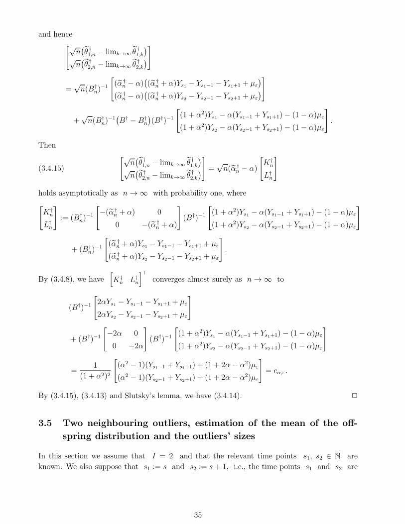
and hence[√
n(θ †1,n − limk→∞ θ †
1,k
)√n(θ †2,n − limk→∞ θ †
2,k
)]
=√n(B†
n)−1
[(α †
n − α)((α †
n + α)Ys1 − Ys1−1 − Ys1+1 + µε
)
(α †n − α)
((α †
n + α)Ys2 − Ys2−1 − Ys2+1 + µε
)]
+√n(B†
n)−1(B† − B†
n
)(B†)−1
[(1 + α2)Ys1 − α(Ys1−1 + Ys1+1)− (1− α)µε
(1 + α2)Ys2 − α(Ys2−1 + Ys2+1)− (1− α)µε
].
Then[√
n(θ †1,n − limk→∞ θ †
1,k
)√n(θ †2,n − limk→∞ θ †
2,k
)]=
√n(α †
n − α)
[K†
n
L†n
](3.4.15)
holds asymptotically as n → ∞ with probability one, where
[K†
n
L†n
]:= (B†
n)−1
[−(α †
n + α) 0
0 −(α †n + α)
](B†)−1
[(1 + α2)Ys1 − α(Ys1−1 + Ys1+1)− (1− α)µε
(1 + α2)Ys2 − α(Ys2−1 + Ys2+1)− (1− α)µε
]
+ (B†n)
−1
[(α †
n + α)Ys1 − Ys1−1 − Ys1+1 + µε
(α †n + α)Ys2 − Ys2−1 − Ys2+1 + µε
].
By (3.4.8), we have[K†
n L†n
]⊤converges almost surely as n → ∞ to
(B†)−1
[2αYs1 − Ys1−1 − Ys1+1 + µε
2αYs2 − Ys2−1 − Ys2+1 + µε
]
+ (B†)−1
[−2α 0
0 −2α
](B†)−1
[(1 + α2)Ys1 − α(Ys1−1 + Ys1+1)− (1− α)µε
(1 + α2)Ys2 − α(Ys2−1 + Ys2+1)− (1− α)µε
]
=1
(1 + α2)2
[(α2 − 1)(Ys1−1 + Ys1+1) + (1 + 2α− α2)µε
(α2 − 1)(Ys2−1 + Ys2+1) + (1 + 2α− α2)µε
]= eα,ε.
By (3.4.15), (3.4.13) and Slutsky’s lemma, we have (3.4.14). 2
3.5 Two neighbouring outliers, estimation of the mean of the off-
spring distribution and the outliers’ sizes
In this section we assume that I = 2 and that the relevant time points s1, s2 ∈ N are
known. We also suppose that s1 := s and s2 := s + 1, i.e., the time points s1 and s2 are
35
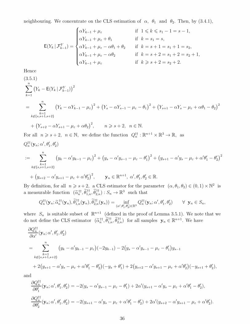
neighbouring. We concentrate on the CLS estimation of α, θ1 and θ2. Then, by (3.4.1),
E(Yk | FYk−1) =
αYk−1 + µε if 1 6 k 6 s1 − 1 = s− 1,
αYk−1 + µε + θ1 if k = s1 = s,
αYk−1 + µε − αθ1 + θ2 if k = s+ 1 = s1 + 1 = s2,
αYk−1 + µε − αθ2 if k = s+ 2 = s1 + 2 = s2 + 1,
αYk−1 + µε if k > s+ 2 = s2 + 2.
Hence
n∑
k=1
(Yk − E(Yk | FY
k−1))2
=n∑
k=1k 6∈s,s+1,s+2
(Yk − αYk−1 − µε
)2+(Ys − αYs−1 − µε − θ1
)2+(Ys+1 − αYs − µε + αθ1 − θ2
)2
+(Ys+2 − αYs+1 − µε + αθ2
)2, n > s+ 2, n ∈ N.
(3.5.1)
For all n > s+ 2, n ∈ N, we define the function Q††n : Rn+1 × R3 → R, as
Q††n (yn;α
′, θ′1, θ′2)
:=n∑
k=1k 6∈s,s+1,s+2
(yk − α′yk−1 − µε
)2+(ys − α′ys−1 − µε − θ′1
)2+(ys+1 − α′ys − µε + α′θ′1 − θ′2
)2
+(ys+2 − α′ys+1 − µε + α′θ′2
)2, yn ∈ R
n+1, α′, θ′1, θ′2 ∈ R.
By definition, for all n > s+2, a CLS estimator for the parameter (α, θ1, θ2) ∈ (0, 1)×N2 is
a measurable function (α ††n , θ ††
1,n, 膆2,n) : Sn → R3 such that
Q††n (yn; α
††n (yn), θ
††1,n(yn), θ
††2,n(yn)) = inf
(α′,θ′1,θ′2)∈R3
Q††n (yn;α
′, θ′1, θ′2) ∀ yn ∈ Sn,
where Sn is suitable subset of Rn+1 (defined in the proof of Lemma 3.5.1). We note that we
do not define the CLS estimator (α ††n , θ ††
1,n, 膆2,n) for all samples yn ∈ Rn+1. We have
∂Q††n
∂α′ (yn;α′, θ′1, θ
′2)
=n∑
k=1k 6∈s,s+1,s+2
(yk − α′yk−1 − µε
)(−2yk−1)− 2
(ys − α′ys−1 − µε − θ′1
)ys−1
+ 2(ys+1 − α′ys − µε + α′θ′1 − θ′2
)(−ys + θ′1) + 2
(ys+2 − α′ys+1 − µε + α′θ′2
)(−ys+1 + θ′2),
and
∂Q††n
∂θ′1(yn;α
′, θ′1, θ′2) = −2(ys − α′ys−1 − µε − θ′1) + 2α′(ys+1 − α′ys − µε + α′θ′1 − θ′2),
∂Q††n
∂θ′2(yn;α
′, θ′1, θ′2) = −2(ys+1 − α′ys − µε + α′θ′1 − θ′2) + 2α′(ys+2 − α′ys+1 − µε + α′θ′2).
36
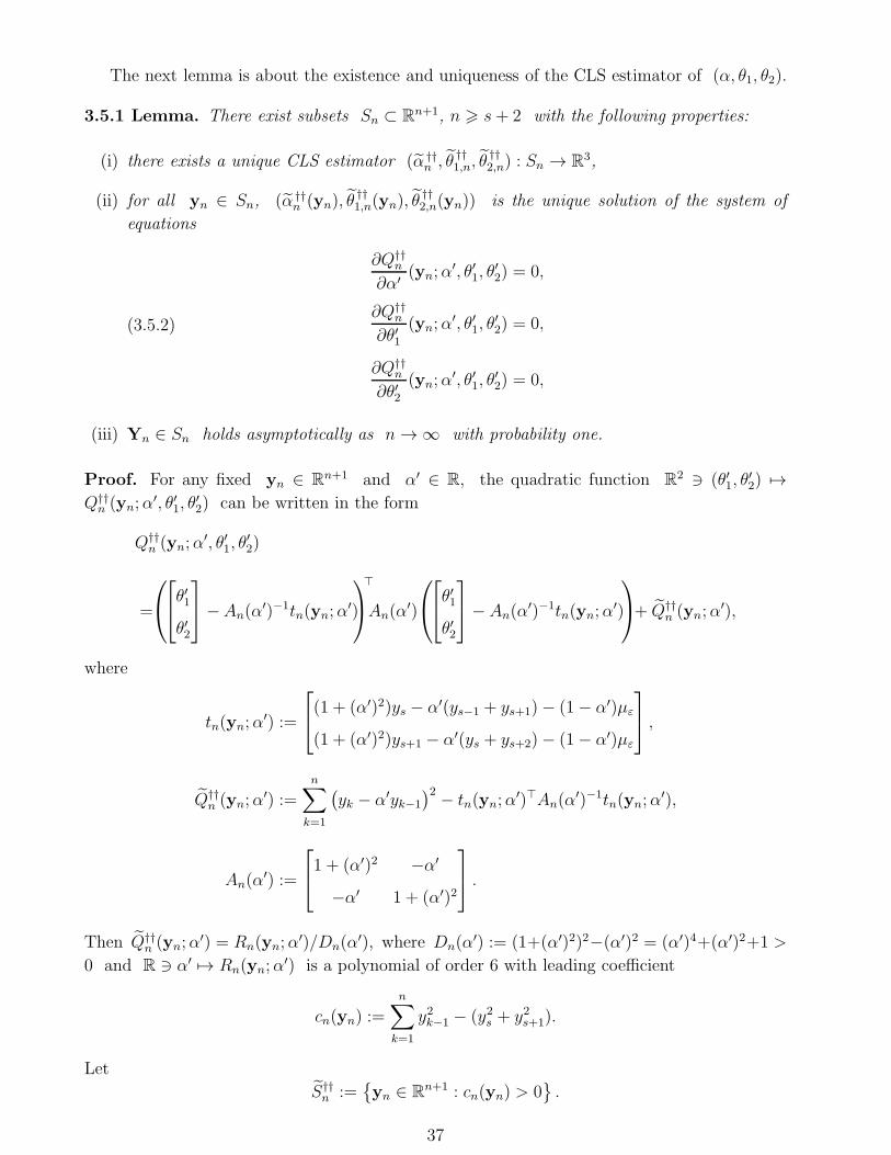
The next lemma is about the existence and uniqueness of the CLS estimator of (α, θ1, θ2).
3.5.1 Lemma. There exist subsets Sn ⊂ Rn+1, n > s+ 2 with the following properties:
(i) there exists a unique CLS estimator (α ††n , θ ††
1,n, 膆2,n) : Sn → R3,
(ii) for all yn ∈ Sn, (α ††n (yn), θ
††1,n(yn), θ
††2,n(yn)) is the unique solution of the system of
equations
∂Q††n
∂α′ (yn;α′, θ′1, θ
′2) = 0,
∂Q††n
∂θ′1(yn;α
′, θ′1, θ′2) = 0,
∂Q††n
∂θ′2(yn;α
′, θ′1, θ′2) = 0,
(3.5.2)
(iii) Yn ∈ Sn holds asymptotically as n → ∞ with probability one.
Proof. For any fixed yn ∈ Rn+1 and α′ ∈ R, the quadratic function R2 ∋ (θ′1, θ′2) 7→
Q††n (yn;α
′, θ′1, θ′2) can be written in the form
Q††n (yn;α
′, θ′1, θ′2)
=
θ
′1
θ′2
−An(α
′)−1tn(yn;α′)
⊤
An(α′)
θ
′1
θ′2
− An(α
′)−1tn(yn;α′)
+ Q††
n (yn;α′),
where
tn(yn;α′) :=
(1 + (α′)2)ys − α′(ys−1 + ys+1)− (1− α′)µε
(1 + (α′)2)ys+1 − α′(ys + ys+2)− (1− α′)µε
,
Q††n (yn;α
′) :=n∑
k=1
(yk − α′yk−1
)2 − tn(yn;α′)⊤An(α
′)−1tn(yn;α′),
An(α′) :=
1 + (α′)2 −α′
−α′ 1 + (α′)2
.
Then Q††n (yn;α
′) = Rn(yn;α′)/Dn(α
′), where Dn(α′) := (1+(α′)2)2−(α′)2 = (α′)4+(α′)2+1 >
0 and R ∋ α′ 7→ Rn(yn;α′) is a polynomial of order 6 with leading coefficient
cn(yn) :=
n∑
k=1
y2k−1 − (y2s + y2s+1).
Let
S††n :=
yn ∈ R
n+1 : cn(yn) > 0.
37
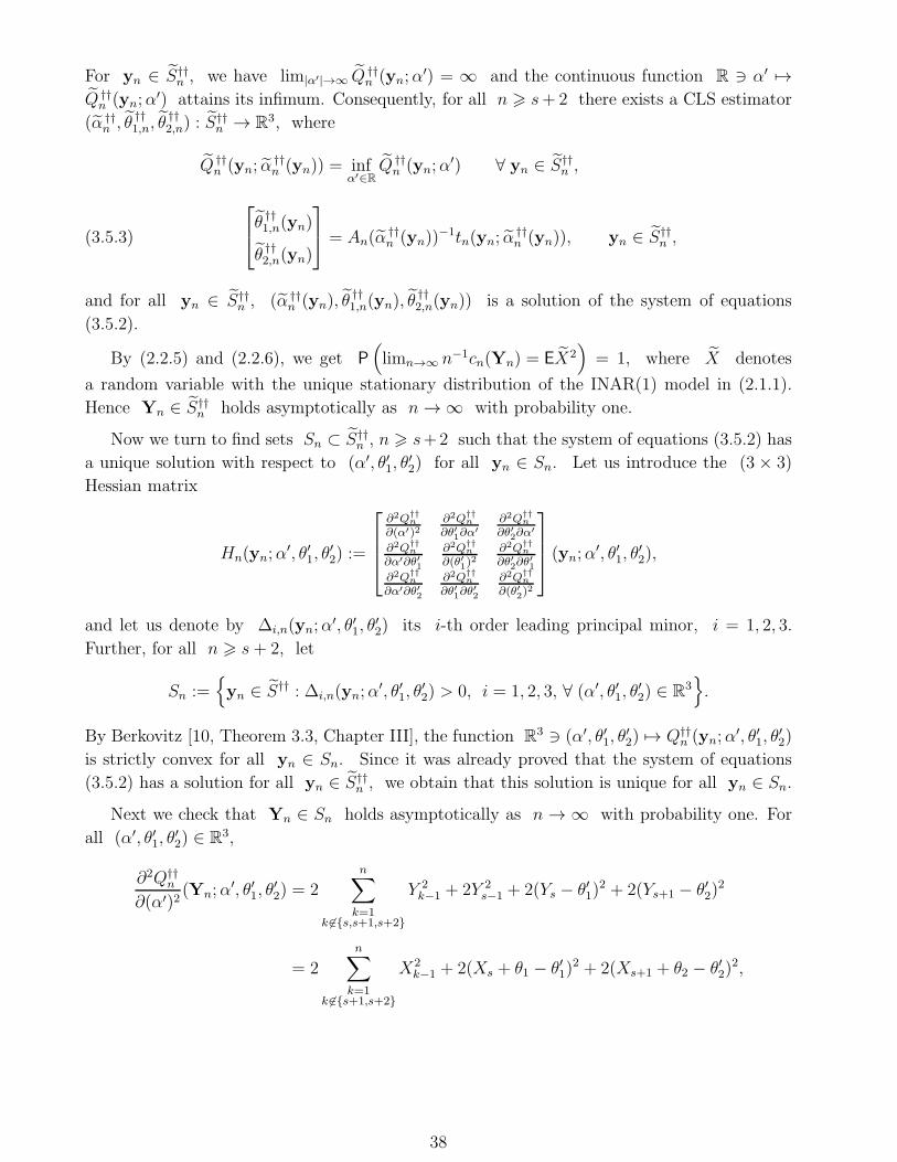
For yn ∈ S††n , we have lim|α′|→∞ Q ††
n (yn;α′) = ∞ and the continuous function R ∋ α′ 7→
Q ††n (yn;α
′) attains its infimum. Consequently, for all n > s+ 2 there exists a CLS estimator
(α ††n , θ ††
1,n, 膆2,n) : S
††n → R3, where
Q ††n (yn; α
††n (yn)) = inf
α′∈RQ ††
n (yn;α′) ∀ yn ∈ S††
n ,
θ
††1,n(yn)
θ ††2,n(yn)
= An(α
††n (yn))
−1tn(yn; ᆆn (yn)), yn ∈ S††
n ,(3.5.3)
and for all yn ∈ S††n , (α ††
n (yn), 膆1,n(yn), θ
††2,n(yn)) is a solution of the system of equations
(3.5.2).
By (2.2.5) and (2.2.6), we get P(limn→∞ n−1cn(Yn) = EX2
)= 1, where X denotes
a random variable with the unique stationary distribution of the INAR(1) model in (2.1.1).
Hence Yn ∈ S††n holds asymptotically as n → ∞ with probability one.
Now we turn to find sets Sn ⊂ S††n , n > s+2 such that the system of equations (3.5.2) has
a unique solution with respect to (α′, θ′1, θ′2) for all yn ∈ Sn. Let us introduce the (3 × 3)
Hessian matrix
Hn(yn;α′, θ′1, θ
′2) :=
∂2Q††n
∂(α′)2∂2Q††
n
∂θ′1∂α′
∂2Q††n
∂θ′2∂α′
∂2Q††n
∂α′∂θ′1
∂2Q††n
∂(θ′1)2
∂2Q††n
∂θ′2∂θ′1
∂2Q††n
∂α′∂θ′2
∂2Q††n
∂θ′1∂θ′2
∂2Q††n
∂(θ′2)2
(yn;α
′, θ′1, θ′2),
and let us denote by ∆i,n(yn;α′, θ′1, θ
′2) its i-th order leading principal minor, i = 1, 2, 3.
Further, for all n > s+ 2, let
Sn :=yn ∈ S†† : ∆i,n(yn;α
′, θ′1, θ′2) > 0, i = 1, 2, 3, ∀ (α′, θ′1, θ
′2) ∈ R
3.
By Berkovitz [10, Theorem 3.3, Chapter III], the function R3 ∋ (α′, θ′1, θ
′2) 7→ Q††
n (yn;α′, θ′1, θ
′2)
is strictly convex for all yn ∈ Sn. Since it was already proved that the system of equations
(3.5.2) has a solution for all yn ∈ S††n , we obtain that this solution is unique for all yn ∈ Sn.
Next we check that Yn ∈ Sn holds asymptotically as n → ∞ with probability one. For
all (α′, θ′1, θ′2) ∈ R
3,
∂2Q††n
∂(α′)2(Yn;α
′, θ′1, θ′2) = 2
n∑
k=1k 6∈s,s+1,s+2
Y 2k−1 + 2Y 2
s−1 + 2(Ys − θ′1)2 + 2(Ys+1 − θ′2)
2
= 2
n∑
k=1k 6∈s+1,s+2
X2k−1 + 2(Xs + θ1 − θ′1)
2 + 2(Xs+1 + θ2 − θ′2)2,
38
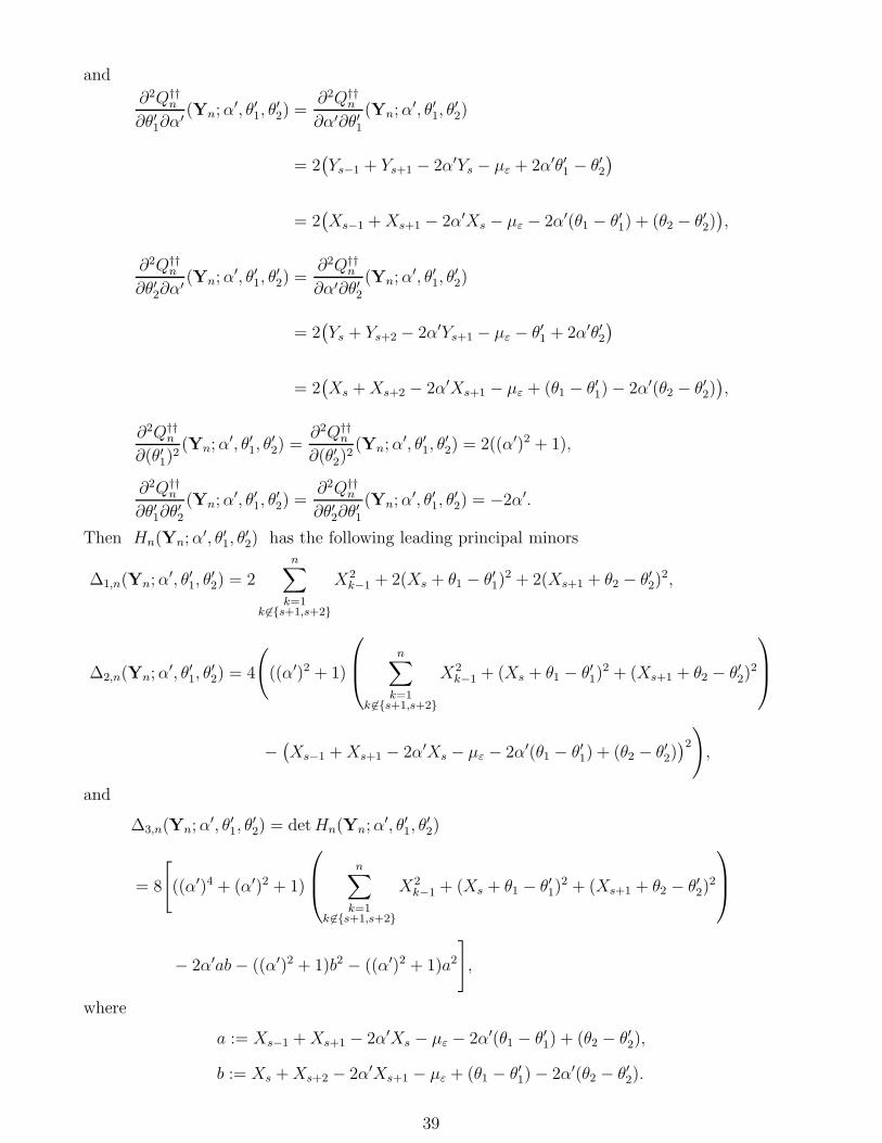
and
∂2Q††n
∂θ′1∂α′ (Yn;α
′, θ′1, θ′2) =
∂2Q††n
∂α′∂θ′1(Yn;α
′, θ′1, θ′2)
= 2(Ys−1 + Ys+1 − 2α′Ys − µε + 2α′θ′1 − θ′2
)
= 2(Xs−1 +Xs+1 − 2α′Xs − µε − 2α′(θ1 − θ′1) + (θ2 − θ′2)
),
∂2Q††n
∂θ′2∂α′ (Yn;α
′, θ′1, θ′2) =
∂2Q††n
∂α′∂θ′2(Yn;α
′, θ′1, θ′2)
= 2(Ys + Ys+2 − 2α′Ys+1 − µε − θ′1 + 2α′θ′2
)
= 2(Xs +Xs+2 − 2α′Xs+1 − µε + (θ1 − θ′1)− 2α′(θ2 − θ′2)
),
∂2Q††n
∂(θ′1)2(Yn;α
′, θ′1, θ′2) =
∂2Q††n
∂(θ′2)2(Yn;α
′, θ′1, θ′2) = 2((α′)2 + 1),
∂2Q††n
∂θ′1∂θ′2
(Yn;α′, θ′1, θ
′2) =
∂2Q††n
∂θ′2∂θ′1
(Yn;α′, θ′1, θ
′2) = −2α′.
Then Hn(Yn;α′, θ′1, θ
′2) has the following leading principal minors
∆1,n(Yn;α′, θ′1, θ
′2) = 2
n∑
k=1k 6∈s+1,s+2
X2k−1 + 2(Xs + θ1 − θ′1)
2 + 2(Xs+1 + θ2 − θ′2)2,
∆2,n(Yn;α′, θ′1, θ
′2) = 4
(((α′)2 + 1)
n∑
k=1k 6∈s+1,s+2
X2k−1 + (Xs + θ1 − θ′1)
2 + (Xs+1 + θ2 − θ′2)2
−(Xs−1 +Xs+1 − 2α′Xs − µε − 2α′(θ1 − θ′1) + (θ2 − θ′2)
)2),
and
∆3,n(Yn;α′, θ′1, θ
′2) = detHn(Yn;α
′, θ′1, θ′2)
= 8
[((α′)4 + (α′)2 + 1)
n∑
k=1k 6∈s+1,s+2
X2k−1 + (Xs + θ1 − θ′1)
2 + (Xs+1 + θ2 − θ′2)2
− 2α′ab− ((α′)2 + 1)b2 − ((α′)2 + 1)a2
],
where
a := Xs−1 +Xs+1 − 2α′Xs − µε − 2α′(θ1 − θ′1) + (θ2 − θ′2),
b := Xs +Xs+2 − 2α′Xs+1 − µε + (θ1 − θ′1)− 2α′(θ2 − θ′2).
39
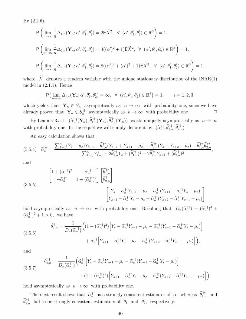
By (2.2.6),
P
(limn→∞
1
n∆1,n(Yn;α
′, θ′1, θ′2) = 2EX2, ∀ (α′, θ′1, θ
′2) ∈ R
3
)= 1,
P
(limn→∞
1
n∆2,n(Yn;α
′, θ′1, θ′2) = 4((α′)2 + 1)EX2, ∀ (α′, θ′1, θ
′2) ∈ R
3
)= 1,
P
(limn→∞
1
n∆3,n(Yn;α
′, θ′1, θ′2) = 8((α′)4 + (α′)2 + 1)EX2, ∀ (α′, θ′1, θ
′2) ∈ R
3
)= 1,
where X denotes a random variable with the unique stationary distribution of the INAR(1)
model in (2.1.1). Hence
P(limn→∞
∆i,n(Yn;α′, θ′1, θ
′2) = ∞, ∀ (α′, θ′1, θ
′2) ∈ R
3)= 1, i = 1, 2, 3,
which yields that Yn ∈ Sn asymptotically as n → ∞ with probability one, since we have
already proved that Yn ∈ S††n asymptotically as n → ∞ with probability one. 2
By Lemma 3.5.1, (α ††n (Yn), θ
††1,n(Yn), θ
††2,n(Yn)) exists uniquely asymptotically as n → ∞
with probability one. In the sequel we will simply denote it by (α ††n , θ ††
1,n, 膆2,n).
An easy calculation shows that
α ††n =
∑nk=1(Yk − µε)Yk−1 − θ ††
1,n(Ys−1 + Ys+1 − µε)− θ ††2,n(Ys + Ys+2 − µε) + θ ††
1,n膆2,n∑n
k=1 Y2k−1 − 2θ ††
1,nYs + (θ ††1,n)
2 − 2θ ††2,nYs+1 + (θ ††
2,n)2
,(3.5.4)
and[1 + (α ††
n )2 −α ††n
−α ††n 1 + (α ††
n )2
][θ ††1,n
θ ††2,n
]
=
[Ys − α ††
n Ys−1 − µε − α ††n (Ys+1 − α ††
n Ys − µε)
Ys+1 − α ††n Ys − µε − α ††
n (Ys+2 − α ††n Ys+1 − µε)
](3.5.5)
hold asymptotically as n → ∞ with probability one. Recalling that Dn(ᆆn ) = (α ††
n )4 +
(α ††n )2 + 1 > 0, we have
θ ††1,n =
1
Dn(ᆆn )
((1 + (α ††
n )2)[Ys − α ††
n Ys−1 − µε − α ††n (Ys+1 − α ††
n Ys − µε)]
+ α ††n
[Ys+1 − α ††
n Ys − µε − α ††n (Ys+2 − α ††
n Ys+1 − µε)])
,
(3.5.6)
and
θ ††2,n =
1
Dn(ᆆn )
(α ††n
[Ys − α ††
n Ys−1 − µε − α ††n (Ys+1 − α ††
n Ys − µε)]
+ (1 + (α ††n )2)
[Ys+1 − α ††
n Ys − µε − α ††n (Ys+2 − α ††
n Ys+1 − µε)])(3.5.7)
hold asymptotically as n → ∞ with probability one.
The next result shows that α ††n is a strongly consistent estimator of α, whereas θ ††
1,n and
θ ††2,n fail to be strongly consistent estimators of θ1 and θ2, respectively.
40
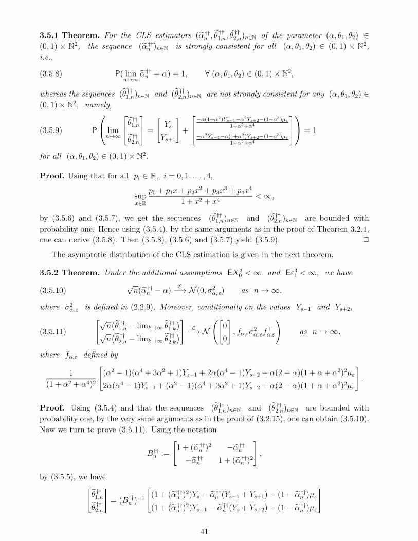
3.5.1 Theorem. For the CLS estimators (α ††n , θ ††
1,n, 膆2,n)n∈N of the parameter (α, θ1, θ2) ∈
(0, 1) × N2, the sequence (α ††n )n∈N is strongly consistent for all (α, θ1, θ2) ∈ (0, 1) × N2,
i.e.,
P( limn→∞
α ††n = α) = 1, ∀ (α, θ1, θ2) ∈ (0, 1)× N
2,(3.5.8)
whereas the sequences (θ ††1,n)n∈N and (θ ††
2,n)n∈N are not strongly consistent for any (α, θ1, θ2) ∈(0, 1)× N
2, namely,
P
lim
n→∞
θ ††1,n
θ ††2,n
=
[Ys
Ys+1
]+
−α(1+α2)Ys−1−α2Ys+2−(1−α3)µε
1+α2+α4
−α2Ys−1−α(1+α2)Ys+2−(1−α3)µε
1+α2+α4
= 1(3.5.9)
for all (α, θ1, θ2) ∈ (0, 1)× N2.
Proof. Using that for all pi ∈ R, i = 0, 1, . . . , 4,
supx∈R
p0 + p1x+ p2x2 + p3x
3 + p4x4
1 + x2 + x4< ∞,
by (3.5.6) and (3.5.7), we get the sequences (θ ††1,n)n∈N and (θ ††
2,n)n∈N are bounded with
probability one. Hence using (3.5.4), by the same arguments as in the proof of Theorem 3.2.1,
one can derive (3.5.8). Then (3.5.8), (3.5.6) and (3.5.7) yield (3.5.9). 2
The asymptotic distribution of the CLS estimation is given in the next theorem.
3.5.2 Theorem. Under the additional assumptions EX30 < ∞ and Eε31 < ∞, we have
√n(α ††
n − α)L−→ N (0, σ2
α, ε) as n → ∞,(3.5.10)
where σ2α, ε is defined in (2.2.9). Moreover, conditionally on the values Ys−1 and Ys+2,
[√n(θ ††1,n − limk→∞ θ ††
1,k
)√n(θ ††2,n − limk→∞ θ ††
2,k
)]
L−→ N([
0
0
], fα,εσ
2α, εf
⊤α,ε
)as n → ∞,(3.5.11)
where fα,ε defined by
1
(1 + α2 + α4)2
[(α2 − 1)(α4 + 3α2 + 1)Ys−1 + 2α(α4 − 1)Ys+2 + α(2− α)(1 + α + α2)2µε
2α(α4 − 1)Ys−1 + (α2 − 1)(α4 + 3α2 + 1)Ys+2 + α(2− α)(1 + α + α2)2µε
].
Proof. Using (3.5.4) and that the sequences (θ ††1,n)n∈N and (θ ††
2,n)n∈N are bounded with
probability one, by the very same arguments as in the proof of (3.2.15), one can obtain (3.5.10).
Now we turn to prove (3.5.11). Using the notation
B††n :=
[1 + (α ††
n )2 −α ††n
−α ††n 1 + (α ††
n )2
],
by (3.5.5), we have[θ ††1,n
θ ††2,n
]= (B††
n )−1
[(1 + (α ††
n )2)Ys − α ††n (Ys−1 + Ys+1)− (1− α ††
n )µε
(1 + (α ††n )2)Ys+1 − α ††
n (Ys + Ys+2)− (1− α ††n )µε
]
41
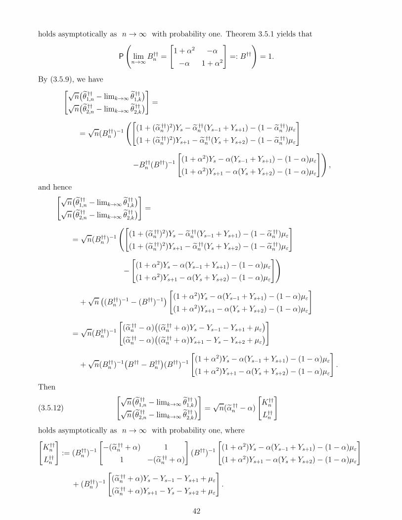
holds asymptotically as n → ∞ with probability one. Theorem 3.5.1 yields that
P
(limn→∞
B††n =
[1 + α2 −α
−α 1 + α2
]=: B††
)= 1.
By (3.5.9), we have[√
n(θ ††1,n − limk→∞ θ ††
1,k
)√n(θ ††2,n − limk→∞ θ ††
2,k
)]=
=√n(B††
n )−1
([(1 + (α ††
n )2)Ys − α ††n (Ys−1 + Ys+1)− (1− α ††
n )µε
(1 + (α ††n )2)Ys+1 − α ††
n (Ys + Ys+2)− (1− α ††n )µε
]
−B††n (B††)−1
[(1 + α2)Ys − α(Ys−1 + Ys+1)− (1− α)µε
(1 + α2)Ys+1 − α(Ys + Ys+2)− (1− α)µε
]),
and hence[√
n(θ ††1,n − limk→∞ θ ††
1,k
)√n(θ ††2,n − limk→∞ θ ††
2,k
)]=
=√n(B††
n )−1
([(1 + (α ††
n )2)Ys − α ††n (Ys−1 + Ys+1)− (1− α ††
n )µε
(1 + (α ††n )2)Ys+1 − α ††
n (Ys + Ys+2)− (1− α ††n )µε
]
−[(1 + α2)Ys − α(Ys−1 + Ys+1)− (1− α)µε
(1 + α2)Ys+1 − α(Ys + Ys+2)− (1− α)µε
])
+√n((B††
n )−1 − (B††)−1)[(1 + α2)Ys − α(Ys−1 + Ys+1)− (1− α)µε
(1 + α2)Ys+1 − α(Ys + Ys+2)− (1− α)µε
]
=√n(B††
n )−1
[(α ††
n − α)((α ††
n + α)Ys − Ys−1 − Ys+1 + µε
)
(α ††n − α)
((α ††
n + α)Ys+1 − Ys − Ys+2 + µε
)]
+√n(B††
n )−1(B†† −B††
n
)(B††)−1
[(1 + α2)Ys − α(Ys−1 + Ys+1)− (1− α)µε
(1 + α2)Ys+1 − α(Ys + Ys+2)− (1− α)µε
].
Then[√
n(θ ††1,n − limk→∞ θ ††
1,k
)√n(θ ††2,n − limk→∞ θ ††
2,k
)]=
√n(α ††
n − α)
[K††
n
L††n
](3.5.12)
holds asymptotically as n → ∞ with probability one, where[K††
n
L††n
]:= (B††
n )−1
[−(α ††
n + α) 1
1 −(α ††n + α)
](B††)−1
[(1 + α2)Ys − α(Ys−1 + Ys+1)− (1− α)µε
(1 + α2)Ys+1 − α(Ys + Ys+2)− (1− α)µε
]
+ (B††n )−1
[(α ††
n + α)Ys − Ys−1 − Ys+1 + µε
(α ††n + α)Ys+1 − Ys − Ys+2 + µε
].
42
By (3.5.8), we have[K††
n L††n
]⊤converges almost surely as n → ∞ to
(B††)−1
[2αYs − Ys−1 − Ys+1 + µε
2αYs+1 − Ys − Ys+2 + µε
]
+ (B††)−1
[−2α 1
1 −2α
](B††)−1
[(1 + α2)Ys − α(Ys−1 + Ys+1)− (1− α)µε
(1 + α2)Ys+1 − α(Ys + Ys+2)− (1− α)µε
]
=1
1 + α2 + α4
[1 + α2 α
α 1 + α2
]([2αYs − Ys−1 − Ys+1 + µε
2αYs+1 − Ys − Ys+2 + µε
]
+1
(1 + α2 + α4)2
[−2α5 − 4α3 1− α2 − 3α4
1− α2 − 3α4 −2α5 − 4α3
][(1 + α2)Ys − α(Ys−1 + Ys+1)− (1− α)µε
(1 + α2)Ys+1 − α(Ys + Ys+2)− (1− α)µε
]),
which is equal to fα,ε, by an easy, but tedious calculation. Hence, by (3.5.12), (3.5.10) and
Slutsky’s lemma, we have (3.5.11). 2
3.6 Two not neighbouring outliers, estimation of the mean of the
offspring and innovation distributions and the outliers’ sizes
In this section we assume that I = 2 and that the relevant time points s1, s2 ∈ N are known.
We also suppose that s1 < s2 − 1, i.e., the time points s1 and s2 are not neighbouring. We
concentrate on the CLS estimation of α, µε, θ1 and θ2.
Motivated by (3.4.2), for all n > s2+1, n ∈ N, we define the function Q†n : Rn+1×R4 → R,
as
Q†n(yn;α
′, µ′ε, θ
′1, θ
′2)
:=
n∑
k=1k 6∈s1,s1+1,s2,s2+1
(yk − α′yk−1 − µ′
ε
)2+(ys1 − α′ys1−1 − µ′
ε − θ′1)2
+(ys1+1 − α′ys1 − µ′
ε + α′θ′1)2
+(ys2 − α′ys2−1 − µ′
ε − θ′2)2
+(ys2+1 − α′ys2 − µ′
ε + α′θ′2)2,
for all yn ∈ Rn+1, α′, µ′ε, θ
′1, θ
′2 ∈ R. By definition, for all n > s2 + 1, a CLS estimator for
the parameter (α, µε, θ1, θ2) ∈ (0, 1)× (0,∞)× N2 is a measurable function
(α †n, µ
†ε,n, θ
†1,n, θ
†2,n) : Sn → R
4
such that
Q†n(yn; α
†n(yn), µ
†ε,n(yn), θ
†1,n(yn), θ
†2,n(yn))
= inf(α′,µ′
ε,θ′1,θ
′2)∈R4
Q†n(yn;α
′, µ′ε, θ
′1, θ
′2) ∀ yn ∈ Sn,
where Sn is suitable subset of Rn+1 (defined in the proof of Lemma 3.6.1). We note that
we do not define the CLS estimator (α †n, µ
†ε,n, θ
†1,n, θ
†2,n) for all samples yn ∈ Rn+1.
The next result is about the existence and uniqueness of (α †n, µ
†ε,n, θ
†1,n, θ
†2,n).
43
3.6.1 Lemma. There exist subsets Sn ⊂ Rn+1, n > max(5, s2 +1) with the following proper-
ties:
(i) there exists a unique CLS estimator (α †n, µ
†ε,n, θ
†1,n, θ
†2,n) : Sn → R4,
(ii) for all yn ∈ Sn, (α †n(yn), µ
†ε,n(yn), θ
†1,n(yn), θ
†2,n(yn)) is the unique solution of the system
of equations
∂Q†n
∂α′ (yn;α′, µ′
ε, θ′1, θ
′2) = 0,
∂Q†n
∂µ′ε
(yn;α′, µ′
ε, θ′1, θ
′2) = 0,
∂Q†n
∂θ′1(yn;α
′, µ′ε, θ
′1, θ
′2) = 0,
∂Q†n
∂θ′2(yn;α
′, µ′ε, θ
′1, θ
′2) = 0,
(3.6.1)
(iii) Yn ∈ Sn holds asymptotically as n → ∞ with probability one.
Proof. For any fixed yn ∈ Rn+1, n > max(5, s2 + 1) and α′ ∈ R, the quadratic function
R3 ∋ (µ′ε, θ
′1, θ
′2) 7→ Q†
n(yn;α′, µ′
ε, θ′1, θ
′2) can be written in the form
Q†n(yn;α
′, µ′ε, θ
′1, θ
′2)
=
µ′ε
θ′1
θ′2
− An(α
′)−1tn(yn;α′)
⊤
An(α′)
µ′ε
θ′1
θ′2
− An(α
′)−1tn(yn;α′)
+ Q†
n(yn;α′),
where
tn(yn;α′) :=
∑nk=1(yk − α′yk−1)
(1 + (α′)2)ys1 − α′(ys1−1 + ys1+1)
(1 + (α′)2)ys2 − α′(ys2−1 + ys2+1)
,
Q†n(yn;α
′) :=n∑
k=1
(yk − α′yk−1
)2 − tn(yn;α′)⊤An(α
′)−1tn(yn;α′),
and the matrix
An(α′) :=
n 1− α′ 1− α′
1− α′ 1 + (α′)2 0
1− α′ 0 1 + (α′)2
is strictly positive definite for all n > 5 and α′ ∈ R. Indeed, the leading principal minors of
An(α′) take the following forms: n,
n(1 + (α′)2)− (1− α′)2 = (n− 1)(α′)2 + 2α′ + n− 1,
Dn(α′) := (1 + (α′)2)
((n− 2)(α′)2 + 4α′ + n− 2
),
44
and for all n > 5, the discriminant 16− 4(n− 2)2 of the equation (n− 2)x2+4x+n− 2 = 0
is negative.
The inverse matrix An(α′)−1 takes the form
1
Dn(α′)
(1 + (α′)2)2 −(1− α′)(1 + (α′)2) −(1− α′)(1 + (α′)2)
−(1 − α′)(1 + (α′)2) n(1 + (α′)2)− (1− α′)2 (1− α′)2
−(1 − α′)(1 + (α′)2) (1− α′)2 n(1 + (α′)2)− (1− α′)2
.
The polynomial R ∋ α′ 7→ Dn(α′) is of order 4 with leading coefficient n − 2. We have
Q†n(yn;α
′) = Rn(yn;α′)/Dn(α
′), where R ∋ α′ 7→ Rn(yn;α′) is a polynomial of order 6 with
leading coefficient
cn(yn) := (n− 2)n∑
k=1
y2k−1 −(
n∑
k=1
yk−1
)2
− (n− 1)(y2s1 + y2s1)
+ 2(ys1 + ys1)n∑
k=1
yk−1 − 2ys1ys1.
Let
S†n :=
yn ∈ R
n+1 : cn(yn) > 0.
For yn ∈ S†n, we have lim|α′|→∞ Q †
n(yn;α′) = ∞ and the continuous function R ∋ α′ 7→
Q †n(yn;α
′) attains its infimum. Consequently, for all n > max(5, s2 + 1) there exists a CLS
estimator (α †n, µ
†ε,n, θ
†1,n, θ
†2,n) : S
†n → R4, where
Q †n(yn; α
†n(yn)) = inf
α′∈RQ †
n(yn;α′) ∀ yn ∈ S†
n,
µ †ε,n(yn)
θ †1,n(yn)
θ †2,n(yn)
= An(α
†n(yn))
−1tn(yn; α†n(yn)), yn ∈ S†
n,(3.6.2)
and for all yn ∈ S†n, (α
†n(yn), µ
†ε,n(yn), θ
†1,n(yn), θ
†2,n(yn)) is a solution of the system of equations
(3.6.1).
By (2.2.5) and (2.2.6), we get P(limn→∞ n−2cn(Yn) = Var X
)= 1, where X denotes
a random variable with the unique stationary distribution of the INAR(1) model in (2.1.1).
Hence Yn ∈ S†n holds asymptotically as n → ∞ with probability one.
Now we turn to find sets Sn ⊂ S†n, n > max(5, s2 + 1) such that the system of equations
(3.6.1) has a unique solution with respect to (α′, µ′ε, θ
′1, θ
′2) for all yn ∈ Sn. Let us introduce
the (4× 4) Hessian matrix
Hn(yn;α′, µ′
ε, θ′1, θ
′2) :=
∂2Q†n
∂(α′)2∂2Q†
n
∂µ′ε∂α
′
∂2Q†n
∂θ′1∂α′
∂2Q†n
∂θ′2∂α′
∂2Q†n
∂α′∂µ′ε
∂2Q†n
∂(µ′ε)
2∂2Q†
n
∂θ′1∂µ′ε
∂2Q†n
∂θ′2∂µ′ε
∂2Q†n
∂α′∂θ′1
∂2Q†n
∂µ′ε∂θ
′1
∂2Q†n
∂(θ′1)2
∂2Q†n
∂θ′2∂θ′1
∂2Q†n
∂α′∂θ′2
∂2Q†n
∂µ′ε∂θ
′2
∂2Q†n
∂θ′1∂θ′2
∂2Q†n
∂(θ′2)2
(yn;α
′, µ′ε, θ
′1, θ
′2),
45
and let us denote by ∆i,n(yn;α′, µ′
ε, θ′1, θ
′2) its i-th order leading principal minor, i = 1, 2, 3, 4.
Further, for all n > max(5, s2 + 1), let
Sn :=yn ∈ S†
n : ∆i,n(yn;α′, µ′
ε, θ′1, θ
′2) > 0, i = 1, 2, 3, 4, ∀ (α′, µ′
ε, θ′1, θ
′2) ∈ R
4.
By Berkovitz [10, Theorem 3.3, Chapter III], the function R4 ∋ (α′, µ′ε, θ
′1, θ
′2) 7→
Q†n(yn;α
′, µ′ε, θ
′1, θ
′2) is strictly convex for all yn ∈ Sn. Since it was already proved that
the system of equations (3.6.1) has a solution for all yn ∈ S†n, we obtain that this solution is
unique for all yn ∈ Sn.
For all yn ∈ Rn+1 and (α′, µ′ε, θ
′1, θ
′2) ∈ R4, we have
∂Q†n
∂α′ (yn;α′, µ′
ε, θ′1, θ
′2)
=n∑
k=1k 6∈s1,s1+1,s2,s2+1
(yk − α′yk−1 − µ′
ε
)(−2yk−1)− 2
(ys1 − α′ys1−1 − µ′
ε − θ′1)ys1−1
+ 2(ys1+1 − α′ys1 − µ′
ε + α′θ′1)(−ys1 + θ′1)− 2
(ys2 − α′ys2−1 − µ′
ε − θ′2)ys2−1
+ 2(ys2+1 − α′ys2 − µ′
ε + α′θ′2)(−ys2 + θ′2),
∂Q†n
∂µ′ε
(yn;α′, µ′
ε, θ′1, θ
′2)
=n∑
k=1k 6∈s1,s1+1,s2,s2+1
(−2)(yk − α′yk−1 − µ′
ε
)− 2(ys1 − α′ys1−1 − µ′
ε − θ′1)
− 2(ys1+1 − α′ys1 − µ′
ε + α′θ′1)− 2(ys2 − α′ys2−1 − µ′
ε − θ′2)
− 2(ys2+1 − α′ys2 − µ′
ε + α′θ′2),
and
∂Q†n
∂θ′i(yn;α
′, µ′ε, θ
′1, θ
′2)
= −2(ysi − α′ysi−1 − µ′ε − θ′i) + 2α′(ysi+1 − α′ysi − µ′
ε + α′θ′i), i = 1, 2.
(3.6.3)
We also get for all (α′, µ′ε, θ
′1, θ
′2) ∈ R
4,
∂2Q†n
∂(α′)2(Yn;α
′, µ′ε, θ
′1, θ
′2)
= 2n∑
k=1k 6∈s1,s1+1,s2,s2+1
Y 2k−1 + 2Y 2
s1−1 + 2(Ys1 − θ′1)2 + 2Y 2
s2−1 + 2(Ys2 − θ′2)2
= 2
n∑
k=1k 6∈s1+1,s2+1
X2k−1 + 2(Xs1 + θ1 − θ′1)
2 + 2(Xs2 + θ2 − θ′2)2,
46
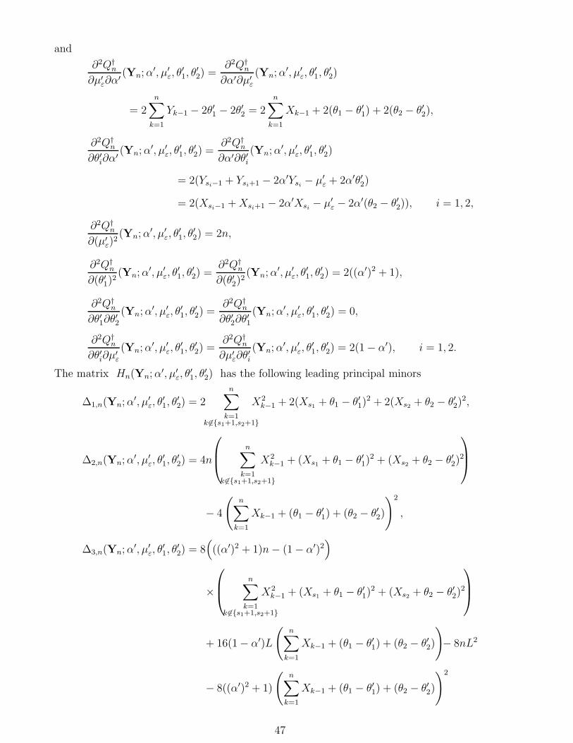
and
∂2Q†n
∂µ′ε∂α
′ (Yn;α′, µ′
ε, θ′1, θ
′2) =
∂2Q†n
∂α′∂µ′ε
(Yn;α′, µ′
ε, θ′1, θ
′2)
= 2
n∑
k=1
Yk−1 − 2θ′1 − 2θ′2 = 2
n∑
k=1
Xk−1 + 2(θ1 − θ′1) + 2(θ2 − θ′2),
∂2Q†n
∂θ′i∂α′ (Yn;α
′, µ′ε, θ
′1, θ
′2) =
∂2Q†n
∂α′∂θ′i(Yn;α
′, µ′ε, θ
′1, θ
′2)
= 2(Ysi−1 + Ysi+1 − 2α′Ysi − µ′ε + 2α′θ′2)
= 2(Xsi−1 +Xsi+1 − 2α′Xsi − µ′ε − 2α′(θ2 − θ′2)), i = 1, 2,
∂2Q†n
∂(µ′ε)
2(Yn;α
′, µ′ε, θ
′1, θ
′2) = 2n,
∂2Q†n
∂(θ′1)2(Yn;α
′, µ′ε, θ
′1, θ
′2) =
∂2Q†n
∂(θ′2)2(Yn;α
′, µ′ε, θ
′1, θ
′2) = 2((α′)2 + 1),
∂2Q†n
∂θ′1∂θ′2
(Yn;α′, µ′
ε, θ′1, θ
′2) =
∂2Q†n
∂θ′2∂θ′1
(Yn;α′, µ′
ε, θ′1, θ
′2) = 0,
∂2Q†n
∂θ′i∂µ′ε
(Yn;α′, µ′
ε, θ′1, θ
′2) =
∂2Q†n
∂µ′ε∂θ
′i
(Yn;α′, µ′
ε, θ′1, θ
′2) = 2(1− α′), i = 1, 2.
The matrix Hn(Yn;α′, µ′
ε, θ′1, θ
′2) has the following leading principal minors
∆1,n(Yn;α′, µ′
ε, θ′1, θ
′2) = 2
n∑
k=1k 6∈s1+1,s2+1
X2k−1 + 2(Xs1 + θ1 − θ′1)
2 + 2(Xs2 + θ2 − θ′2)2,
∆2,n(Yn;α′, µ′
ε, θ′1, θ
′2) = 4n
n∑
k=1k 6∈s1+1,s2+1
X2k−1 + (Xs1 + θ1 − θ′1)
2 + (Xs2 + θ2 − θ′2)2
− 4
(n∑
k=1
Xk−1 + (θ1 − θ′1) + (θ2 − θ′2)
)2
,
∆3,n(Yn;α′, µ′
ε, θ′1, θ
′2) = 8
(((α′)2 + 1)n− (1− α′)2
)
×
n∑
k=1k 6∈s1+1,s2+1
X2k−1 + (Xs1 + θ1 − θ′1)
2 + (Xs2 + θ2 − θ′2)2
+ 16(1− α′)L
(n∑
k=1
Xk−1 + (θ1 − θ′1) + (θ2 − θ′2)
)− 8nL2
− 8((α′)2 + 1)
(n∑
k=1
Xk−1 + (θ1 − θ′1) + (θ2 − θ′2)
)2
47
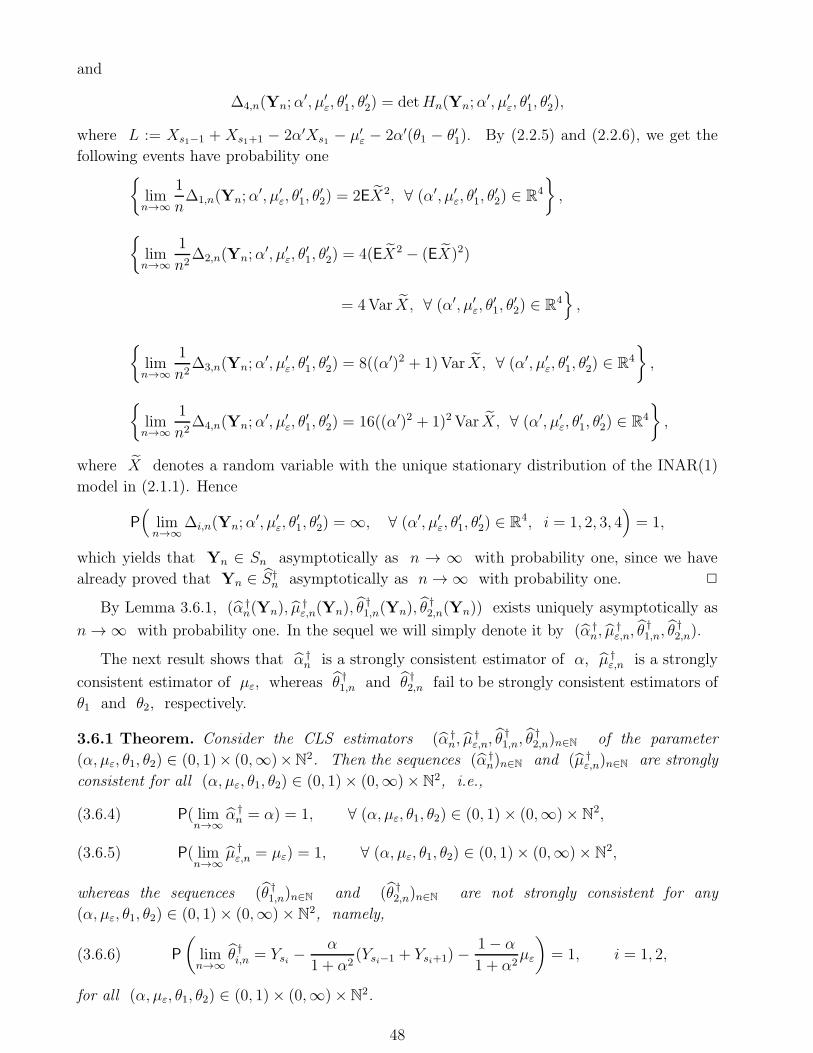
and
∆4,n(Yn;α′, µ′
ε, θ′1, θ
′2) = detHn(Yn;α
′, µ′ε, θ
′1, θ
′2),
where L := Xs1−1 + Xs1+1 − 2α′Xs1 − µ′ε − 2α′(θ1 − θ′1). By (2.2.5) and (2.2.6), we get the
following events have probability onelimn→∞
1
n∆1,n(Yn;α
′, µ′ε, θ
′1, θ
′2) = 2EX2, ∀ (α′, µ′
ε, θ′1, θ
′2) ∈ R
4
,
limn→∞
1
n2∆2,n(Yn;α
′, µ′ε, θ
′1, θ
′2) = 4(EX2 − (EX)2)
= 4Var X, ∀ (α′, µ′ε, θ
′1, θ
′2) ∈ R
4,
limn→∞
1
n2∆3,n(Yn;α
′, µ′ε, θ
′1, θ
′2) = 8((α′)2 + 1)Var X, ∀ (α′, µ′
ε, θ′1, θ
′2) ∈ R
4
,
limn→∞
1
n2∆4,n(Yn;α
′, µ′ε, θ
′1, θ
′2) = 16((α′)2 + 1)2Var X, ∀ (α′, µ′
ε, θ′1, θ
′2) ∈ R
4
,
where X denotes a random variable with the unique stationary distribution of the INAR(1)
model in (2.1.1). Hence
P(
limn→∞
∆i,n(Yn;α′, µ′
ε, θ′1, θ
′2) = ∞, ∀ (α′, µ′
ε, θ′1, θ
′2) ∈ R
4, i = 1, 2, 3, 4)= 1,
which yields that Yn ∈ Sn asymptotically as n → ∞ with probability one, since we have
already proved that Yn ∈ S†n asymptotically as n → ∞ with probability one. 2
By Lemma 3.6.1, (α †n(Yn), µ
†ε,n(Yn), θ
†1,n(Yn), θ
†2,n(Yn)) exists uniquely asymptotically as
n → ∞ with probability one. In the sequel we will simply denote it by (α †n, µ
†ε,n, θ
†1,n, θ
†2,n).
The next result shows that α †n is a strongly consistent estimator of α, µ †
ε,n is a strongly
consistent estimator of µε, whereas θ †1,n and θ †
2,n fail to be strongly consistent estimators of
θ1 and θ2, respectively.
3.6.1 Theorem. Consider the CLS estimators (α †n, µ
†ε,n, θ
†1,n, θ
†2,n)n∈N of the parameter
(α, µε, θ1, θ2) ∈ (0, 1)× (0,∞)×N2. Then the sequences (α †n)n∈N and (µ †
ε,n)n∈N are strongly
consistent for all (α, µε, θ1, θ2) ∈ (0, 1)× (0,∞)× N2, i.e.,
P( limn→∞
α †n = α) = 1, ∀ (α, µε, θ1, θ2) ∈ (0, 1)× (0,∞)× N
2,(3.6.4)
P( limn→∞
µ †ε,n = µε) = 1, ∀ (α, µε, θ1, θ2) ∈ (0, 1)× (0,∞)× N
2,(3.6.5)
whereas the sequences (θ †1,n)n∈N and (θ †
2,n)n∈N are not strongly consistent for any
(α, µε, θ1, θ2) ∈ (0, 1)× (0,∞)× N2, namely,
P
(limn→∞
θ †i,n = Ysi −
α
1 + α2(Ysi−1 + Ysi+1)−
1− α
1 + α2µε
)= 1, i = 1, 2,(3.6.6)
for all (α, µε, θ1, θ2) ∈ (0, 1)× (0,∞)× N2.
48
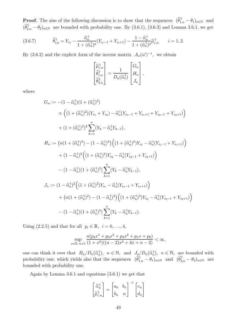
Proof. The aim of the following discussion is to show that the sequences (θ †1,n − θ1)n∈N and
(θ †2,n − θ2)n∈N are bounded with probability one. By (3.6.1), (3.6.3) and Lemma 3.6.1, we get
θ †i,n = Ysi −
α †n
1 + (α †n)2
(Ysi−1 + Ysi+1)−1− α †
n
1 + (α †n)2
µ †ε,n i = 1, 2.(3.6.7)
By (3.6.2) and the explicit form of the inverse matrix An(α′)−1, we obtain
µ †ε,n
θ †1,n
θ †2,n
=
1
Dn(α†n)
Gn
Hn
Jn
,
where
Gn := −(1− α †n)(1 + (α †
n)2)
×((1 + (α †
n)2)(Ys1 + Ys2)− α †
n(Ys1−1 + Ys1+1 + Ys2−1 + Ys2+1))
+ (1 + (α †n)
2)2n∑
k=1
(Yk − α †nYk−1),
Hn :=(n(1 + (α †
n)2)− (1− α †
n)2)(
(1 + (α †n)
2)Ys1 − α †n(Ys1−1 + Ys1+1)
)
+ (1− α †n)
2((1 + (α †
n)2)Ys2 − α †
n(Ys2−1 + Ys2+1))
− (1− α †n)(1 + (α †
n)2)
n∑
k=1
(Yk − α †nYk−1),
Jn := (1− α †n)
2((1 + (α †
n)2)Ys1 − α †
n(Ys1−1 + Ys1+1))
+(n(1 + (α †
n)2)− (1− α †
n)2)(
(1 + (α †n)
2)Ys2 − α †n(Ys2−1 + Ys2+1)
)
− (1− α †n)(1 + (α †
n)2)
n∑
k=1
(Yk − α †nYk−1).
Using (2.2.5) and that for all pi ∈ R, i = 0, . . . , 4,
supx∈R, n>5
n(p4x4 + p3x
3 + p2x2 + p1x+ p0)
(1 + x2)((n− 2)x2 + 4x+ n− 2)< ∞,
one can think it over that Hn/Dn(α†n), n ∈ N, and Jn/Dn(α
†n), n ∈ N, are bounded with
probability one, which yields also that the sequences (θ †1,n − θ1)n∈N and (θ †
2,n − θ2)n∈N are
bounded with probability one.
Again by Lemma 3.6.1 and equations (3.6.1) we get that
[α †n
µ †ε,n
]=
[an bn
bn n
]−1 [cn
dn
]
49
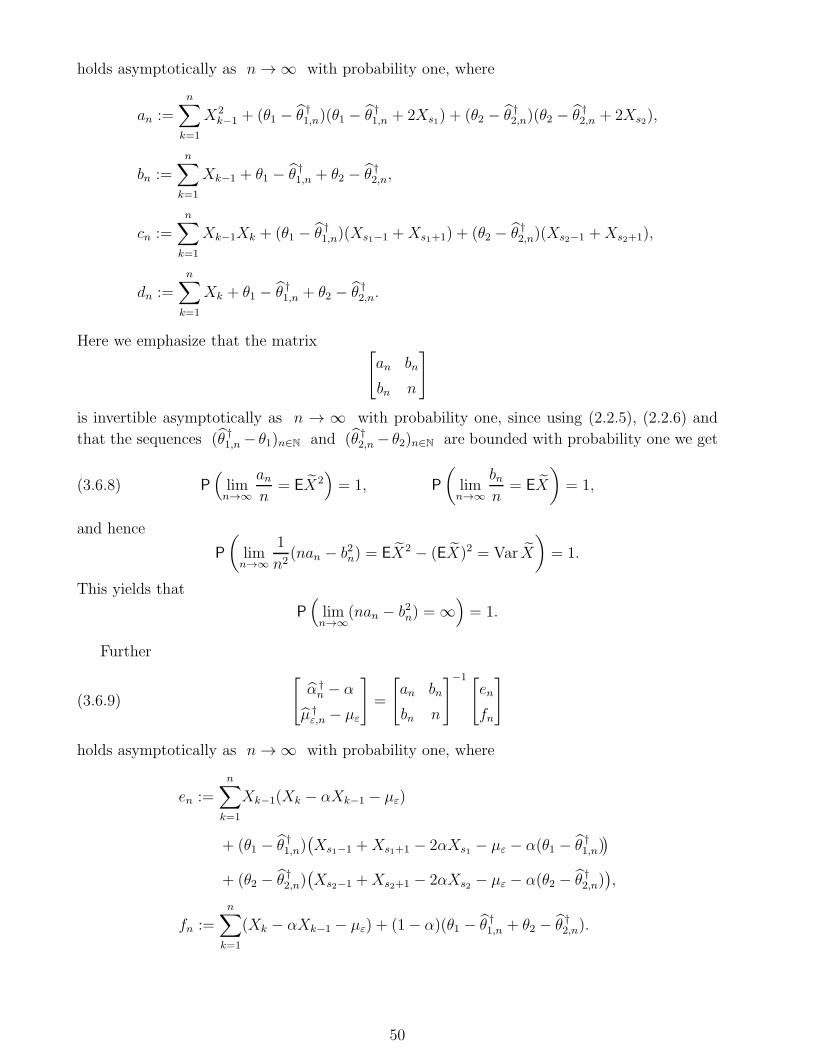
holds asymptotically as n → ∞ with probability one, where
an :=
n∑
k=1
X2k−1 + (θ1 − θ †
1,n)(θ1 − θ †1,n + 2Xs1) + (θ2 − θ †
2,n)(θ2 − θ †2,n + 2Xs2),
bn :=
n∑
k=1
Xk−1 + θ1 − θ †1,n + θ2 − θ †
2,n,
cn :=n∑
k=1
Xk−1Xk + (θ1 − θ †1,n)(Xs1−1 +Xs1+1) + (θ2 − θ †
2,n)(Xs2−1 +Xs2+1),
dn :=n∑
k=1
Xk + θ1 − θ †1,n + θ2 − θ †
2,n.
Here we emphasize that the matrix [an bn
bn n
]
is invertible asymptotically as n → ∞ with probability one, since using (2.2.5), (2.2.6) and
that the sequences (θ †1,n − θ1)n∈N and (θ †
2,n − θ2)n∈N are bounded with probability one we get
P(limn→∞
ann
= EX2)= 1, P
(limn→∞
bnn
= EX
)= 1,(3.6.8)
and hence
P
(limn→∞
1
n2(nan − b2n) = EX2 − (EX)2 = Var X
)= 1.
This yields that
P(limn→∞
(nan − b2n) = ∞)= 1.
Further
[α †n − α
µ †ε,n − µε
]=
[an bn
bn n
]−1 [en
fn
](3.6.9)
holds asymptotically as n → ∞ with probability one, where
en :=n∑
k=1
Xk−1(Xk − αXk−1 − µε)
+ (θ1 − θ †1,n)(Xs1−1 +Xs1+1 − 2αXs1 − µε − α(θ1 − θ †
1,n))
+ (θ2 − θ †2,n)(Xs2−1 +Xs2+1 − 2αXs2 − µε − α(θ2 − θ †
2,n)),
fn :=n∑
k=1
(Xk − αXk−1 − µε) + (1− α)(θ1 − θ †1,n + θ2 − θ †
2,n).
50
Then, using again (2.2.3), (2.2.5), (2.2.6), (2.2.7) and that the sequences (θ †1,n−θ1)n∈N and
(θ †2,n − θ2)n∈N are bounded with probability one, we get
P(limn→∞
enn
= αEX2 + µεEX − αEX2 − µεEX = 0)= 1,
P
(limn→∞
fnn
= EX − αEX − µε = 0
)= 1.
Hence, by (3.6.9), we obtain
P
lim
n→∞
[α †n − α
µ †ε,n − µε
]=
[EX2 EX
EX 1
]−1 [0
0
]=
[0
0
] = 1,
which yields (3.6.4) and (3.6.5). Then (3.6.4), (3.6.5) and (3.6.7) imply (3.6.6). 2
The asymptotic distribution of the CLS estimation is given in the next theorem.
3.6.2 Theorem. Under the additional assumptions EX30 < ∞ and Eε31 < ∞, we have
[ √n(α †
n − α)√n(µ †
ε,n − µε)
]L−→ N
([0
0
], Bα, ε
)as n → ∞,(3.6.10)
where Bα,ε is defined in (2.3.2). Moreover, conditionally on the values Ys1−1, Ys2−1 and
Ys1+1, Ys2+1,
[√n(θ †1,n − limk→∞ θ †
1,k
)√n(θ †2,n − limk→∞ θ †
2,k
)]
L−→ N([
0
0
], Cα,εBα,εC
⊤α,ε
)as n → ∞,(3.6.11)
where
Cα,ε :=1
(1 + α2)2
[(α2 − 1)(Ys1−1 + Ys1+1) + (1 + 2α− α2)µε (α− 1)(1 + α2)
(α2 − 1)(Ys2−1 + Ys2+1) + (1 + 2α− α2)µε (α− 1)(1 + α2)
].
Proof. By (2.3.2) and (3.6.9), to prove (3.6.10) it is enough to show that
P
(limn→∞
1
n
[an bn
bn n
]=
[EX2 EX
EX 1
])= 1,(3.6.12)
1√n
[en
fn
]L−→ N
([0
0
], Aα,ε
)as n → ∞,(3.6.13)
where X is a random variable having the unique stationary distribution of the INAR(1) model
in (2.1.1) and the (2× 2)-matrix Aα,ε is defined in (2.3.3). By (3.6.8), we have (3.6.12). By
formula (6.43) in Hall and Heyde [35, Section 6.3],
[1√n
∑nk=1Xk−1(Xk − αXk−1 − µε)
1√n
∑nk=1(Xk − αXk−1 − µε)
]L−→ N
([0
0
], Aα,ε
)as n → ∞.
51
Hence using that the sequences (θ †1,n−θ1)n∈N and (θ †
2,n−θ2)n∈N are bounded with probability
one, by Slutsky’s lemma (see, e.g., Lemma 2.8 in van der Vaart [63]), we get (3.6.13).
Now we turn to prove (3.6.11). Using the notation
B†n :=
[1 + (α †
n)2 0
0 1 + (α †n)
2
],
by (3.6.7), we have
θ
†1,n
θ †2,n
= (B†
n)−1
(1 + (α †
n)2)Ys1 − α †
n(Ys1−1 + Ys1+1)− (1− α †n)µ
†ε,n
(1 + (α †n)
2)Ys2 − α †n(Ys2−1 + Ys2+1)− (1− α †
n)µ†ε,n
holds asymptotically as n → ∞ with probability one. Theorem 3.6.1 yields that
P
(limn→∞
B†n =
[1 + α2 0
0 1 + α2
]=: B†
)= 1.
By (3.6.6), we have
√n(θ †1,n − limk→∞ θ †
1,k
)
√n(θ †2,n − limk→∞ θ †
2,k
)
=√n(B†
n)−1
(1 + (α †
n)2)Ys1 − α †
n(Ys1−1 + Ys1+1)− (1− α †n)µ
†ε,n
(1 + (α †n)
2)Ys2 − α †n(Ys2−1 + Ys2+1)− (1− α †
n)µ†ε,n
−B†n(B
†)−1
(1 + α2)Ys1 − α(Ys1−1 + Ys1+1)− (1− α)µε
(1 + α2)Ys2 − α(Ys2−1 + Ys2+1)− (1− α)µε
=√n(B†
n)−1
(1 + (α †
n)2)Ys1 − α †
n(Ys1−1 + Ys1+1)− (1− α †n)µ
†ε,n
(1 + (α †n)
2)Ys2 − α †n(Ys2−1 + Ys2+1)− (1− α †
n)µ†ε,n
−
(1 + α2)Ys1 − α(Ys1−1 + Ys1+1)− (1− α)µε
(1 + α2)Ys2 − α(Ys2−1 + Ys2+1)− (1− α)µε
+√n((B†
n)−1 − (B†)−1
)(1 + α2)Ys1 − α(Ys1−1 + Ys1+1)− (1− α)µε
(1 + α2)Ys2 − α(Ys2−1 + Ys2+1)− (1− α)µε
=√n(B†
n)−1
(α
†n + α)Ys1 − (Ys1−1 + Ys1+1) + µ †
ε,n α− 1
(α †n + α)Ys2 − (Ys2−1 + Ys2+1) + µ †
ε,n α− 1
α †
n − α
µ †ε,n − µε
+√n(B†
n)−1(B† −B†
n
)(B†)−1
(1 + α2)Ys1 − α(Ys1−1 + Ys1+1)− (1− α)µε
(1 + α2)Ys2 − α(Ys2−1 + Ys2+1)− (1− α)µε
.
52
Then√n(θ †1,n − limk→∞ θ †
1,k
)
√n(θ †2,n − limk→∞ θ †
2,k
)
= Cn,α,ε
√n(α †
n − α)√n(µ †
ε,n − µε)
(3.6.14)
holds asymptotically as n → ∞ with probability one, where Cn,α,ε is defined by
(B†n)
−1
(α
†n + α)Ys1 − Ys1−1 − Ys1+1 + µ †
ε,n α− 1
(α †n + α)Ys2 − Ys2−1 − Ys2+1 + µ †
ε,n α− 1
− (α †n + α)(B†
n)−1(B†)−1
(1 + α2)Ys1 − α(Ys1−1 + Ys1+1)− (1− α)µε 0
(1 + α2)Ys2 − α(Ys2−1 + Ys2+1)− (1− α)µε 0
.
By (3.6.4) and (3.6.5), we have Cn,α,ε converges almost surely as n → ∞ to
(B†)−1
2αYs1 − Ys1−1 − Ys1+1 + µε α− 1
2αYs2 − Ys2−1 − Ys2+1 + µε α− 1
+ (B†)−1
[−2α 0
0 −2α
](B†)−1
(1 + α2)Ys1 − α(Ys1−1 + Ys1+1)− (1− α)µε 0
(1 + α2)Ys2 − α(Ys2−1 + Ys2+1)− (1− α)µε 0
=1
(1 + α2)2
(α
2 − 1)(Ys1−1 + Ys1+1) + (1 + 2α− α2)µε (α− 1)(1 + α2)
(α2 − 1)(Ys2−1 + Ys2+1) + (1 + 2α− α2)µε (α− 1)(1 + α2)
= Cα,ε.
By (3.6.14), (3.6.10) and Slutsky’s lemma, we have (3.6.11). 2
3.7 Two neighbouring outliers, estimation of the mean of the off-
spring and innovation distributions and the outliers’ sizes
In this section we assume that I = 2 and that the relevant time points s1, s2 ∈ N are
known. We also suppose that s1 := s and s2 := s + 1, i.e., the time points s1 and s2 are
neighbouring. We concentrate on the CLS estimation of α, µε, θ1 and θ2.
Motivated by (3.5.1), for all n > s+2, n ∈ N, we define the function Q††n : Rn+1×R4 → R,
as
Q††n (yn;α
′, µ′ε, θ
′1, θ
′2)
:=
n∑
k=1k 6∈s,s+1,s+2
(yk − α′yk−1 − µ′
ε
)2+(ys − α′ys−1 − µ′
ε − θ′1)2
+(ys+1 − α′ys − µ′
ε + α′θ′1 − θ′2)2
+(ys+2 − α′ys+1 − µ′
ε + α′θ′2)2, yn ∈ R
n+1, α′, µ′ε, θ
′1, θ
′2 ∈ R.
53
By definition, for all n > s + 2, a CLS estimator for the parameter (α, µε, θ1, θ2) ∈ (0, 1)×(0,∞)× N2 is a measurable function (α ††
n , µ ††ε,n, θ
††1,n, θ
††2,n) : Sn → R4 such that
Q††n (yn; α
††n (yn),µ
††ε,n(yn), θ
††1,n(yn), θ
††2,n(yn))
= inf(α′,µ′
ε,θ′1,θ
′2)∈R4
Q††n (yn;α
′, µ′ε, θ
′1, θ
′2) ∀ yn ∈ Sn,
where Sn is suitable subset of Rn+1 (defined in the proof of Lemma 3.7.1). We note that
we do not define the CLS estimator (α ††n , µ ††
ε,n, 膆1,n, θ
††2,n) for all samples yn ∈ R
n+1. For all
yn ∈ Rn+1 and (α′, µ′ε, θ
′1, θ
′2) ∈ R4,
∂Q††n
∂α′ (yn;α′, µ′
ε, θ′1, θ
′2)
=n∑
k=1k 6∈s,s+1,s+2
(yk − α′yk−1 − µ′
ε
)(−2yk−1)− 2
(ys − α′ys−1 − µ′
ε − θ′1)ys−1
+ 2(ys+1 − α′ys − µ′
ε + α′θ′1 − θ′2)(−ys + θ′1) + 2
(ys+2 − α′ys+1 − µ′
ε + α′θ′2)(−ys+1 + θ′2),
and
∂Q††n
∂µ′ε
(yn;α′, µ′
ε, θ′1, θ
′2)
=
n∑
k=1k 6∈s,s+1,s+2
(−2)(yk − α′yk−1 − µ′
ε
)− 2(ys − α′ys−1 − µ′
ε − θ′1)
− 2(ys+1 − α′ys − µ′
ε + α′θ′1 − θ′2)− 2(ys+2 − α′ys+1 − µ′
ε + α′θ′2),
∂Q††n
∂θ′1(yn;α
′, µ′ε, θ
′1, θ
′2)
= −2(ys − α′ys−1 − µ′ε − θ′1) + 2α′(ys+1 − α′ys − µ′
ε + α′θ′1 − θ′2),
∂Q††n
∂θ′2(yn;α
′, µ′ε, θ
′1, θ
′2)
= −2(ys+1 − α′ys − µ′ε + α′θ′1 − θ′2) + 2α′(ys+2 − α′ys+1 − µ′
ε + α′θ′2).
The next lemma is about the existence and uniqueness of the CLS estimator of (α, µε, θ1, θ2).
3.7.1 Lemma. There exist subsets Sn ⊂ Rn+1, n > max(3, s+2) with the following properties:
(i) there exists a unique CLS estimator (α ††n , µ ††
ε,n, 膆1,n, θ
††2,n) : Sn → R4,
(ii) for all yn ∈ Sn, (α ††n (yn), µ
††ε,n(yn), θ
††1,n(yn), θ
††2,n(yn)) is the unique solution of the system
of equations
∂Q††n
∂α′ (yn;α′, µ′
ε, θ′1, θ
′2) = 0,
∂Q††n
∂µ′ε
(yn;α′, µ′
ε, θ′1, θ
′2) = 0,
∂Q††n
∂θ′1(yn;α
′, µ′ε, θ
′1, θ
′2) = 0,
∂Q††n
∂θ′2(yn;α
′, µ′ε, θ
′1, θ
′2) = 0,
(3.7.1)
54
(iii) Yn ∈ Sn holds asymptotically as n → ∞ with probability one.
Proof. For any fixed yn ∈ Rn+1, n > max(3, s + 2) and α′ ∈ R, the quadratic function
R3 ∋ (µ′ε, θ
′1, θ
′2) 7→ Q††
n (yn;α′, µ′
ε, θ′1, θ
′2) can be written in the form
Q††n (yn;α
′, µ′ε, θ
′1, θ
′2)
=
µ′ε
θ′1
θ′2
−An(α
′)−1tn(yn;α′)
⊤
An(α′)
µ′ε
θ′1
θ′2
−An(α
′)−1tn(yn;α′)
+ Q††
n (yn;α′),
where
tn(yn;α′) :=
∑nk=1(yk − α′yk−1)
(1 + (α′)2)ys − α′(ys−1 + ys+1)
(1 + (α′)2)ys+1 − α′(ys + ys+2)
,
Q††n (yn;α
′) :=
n∑
k=1
(yk − α′yk−1
)2 − tn(yn;α′)⊤An(α
′)−1tn(yn;α′),
and the matrix
An(α′) :=
n 1− α′ 1− α′
1− α′ 1 + (α′)2 −α′
1− α′ −α′ 1 + (α′)2
is strictly positive definite for all n > 3 and α′ ∈ R. Indeed, the leading principal minors of
An(α′) take the following forms: n,
n(1 + (α′)2)− (1− α′)2 = (n− 1)(α′)2 + 2α′ + n− 1,
Dn(α′) := n(1 + (α′)2)2 − 2(1− α′)2(1 + (α′)2)− 2α′(1− α′)2 − n(α′)2
= n(1 + α′ + (α′)2)(1− α′ + (α′)2)− 2(1− α′)2(1 + α′ + (α′)2)
= (1 + α′ + (α′)2)((n− 2)(α′)2 − (n− 4)α′ + n− 2
),
and for all n > 3, the discriminant (n − 4)2 − 4(n − 2)2 = −3n2 + 8n of the equation
(n− 2)x2 − (n− 4)x+ n− 2 = 0 is negative. The inverse matrix An(α′)−1 takes the form
1
Dn(α′)
1 + (α′)2 + (α′)4 −(1 − α′)(1 + α′ + (α′)2) −(1− α′)(1 + α′ + (α′)2)
−(1− α′)(1 + α′ + (α′)2) n(1 + (α′)2)− (1− α′)2 (1− α′)2 + nα′
−(1− α′)(1 + α′ + (α′)2) (1− α′)2 + nα′ n(1 + (α′)2)− (1− α′)2
.
The polynomial R ∋ α′ 7→ Dn(α′) is of order 4 with leading coefficient n − 2. We have
Q††n (yn;α
′) = Rn(yn;α′)/Dn(α
′), where R ∋ α′ 7→ Rn(yn;α′) is a polynomial of order 6 with
55
leading coefficient
cn(yn) := (n− 2)n∑
k=1
y2k−1 −(
n∑
k=1
yk−1
)2
− (n− 1)(y2s + y2s+1)
+ 2(ys + ys+1)n∑
k=1
yk−1 − 2ysys+1.
Let
S ††n :=
yn ∈ R
n+1 : cn(yn) > 0.
For yn ∈ S ††n , we have lim|α′|→∞ Q ††
n (yn;α′) = ∞ and the continuous function R ∋ α′ 7→
Q ††n (yn;α
′) attains its infimum. Consequently, for all n > max(3, s + 2) there exists a CLS
estimator (α ††n , µ ††
ε,n, 膆1,n, θ
††2,n) : S
††n → R4, where
Q ††n (yn; α
††n (yn)) = inf
α′∈RQ ††
n (yn;α′) ∀ yn ∈ S ††
n ,
µ ††ε,n(yn)
θ ††1,n(yn)
θ ††2,n(yn)
= An(α
††n (yn))
−1tn(yn; ᆆn (yn)), yn ∈ S ††
n ,(3.7.2)
and for all yn ∈ S††n , (α ††
n (yn), µ††ε,n(yn), θ
††1,n(yn), θ
††2,n(yn)) is a solution of the system of
equations (3.7.1).
By (2.2.5) and (2.2.6), we get P(limn→∞ n−2cn(Yn) = Var X
)= 1, where X denotes
a random variable with the unique stationary distribution of the INAR(1) model in (2.1.1).
Hence Yn ∈ S ††n holds asymptotically as n → ∞ with probability one.
Now we turn to find sets Sn ⊂ S††n , n > max(3, s + 2) such that the system of equations
(3.7.1) has a unique solution with respect to (α′, µ′ε, θ
′1, θ
′2) for all yn ∈ Sn. Let us introduce
the (4× 4) Hessian matrix
Hn(yn;α′, µ′
ε, θ′1, θ
′2) :=
∂2Q†n
∂(α′)2∂2Q†
n
∂µ′ε∂α
′
∂2Q†n
∂θ′1∂α′
∂2Q†n
∂θ′2∂α′
∂2Q†n
∂α′∂µ′ε
∂2Q†n
∂(µ′ε)
2∂2Q†
n
∂θ′1∂µ′ε
∂2Q†n
∂θ′2∂µ′ε
∂2Q†n
∂α′∂θ′1
∂2Q†n
∂µ′ε∂θ
′1
∂2Q†n
∂(θ′1)2
∂2Q†n
∂θ′2∂θ′1
∂2Q†n
∂α′∂θ′2
∂2Q†n
∂µ′ε∂θ
′2
∂2Q†n
∂θ′1∂θ′2
∂2Q†n
∂(θ′2)2
(yn;α
′, µ′ε, θ
′1, θ
′2),
and let us denote by ∆i,n(yn;α′, µ′
ε, θ′1, θ
′2) its i-th order leading principal minor, i = 1, 2, 3, 4.
Further, for all n > max(3, s+ 2), let
Sn :=yn ∈ S††
n : ∆i,n(yn;α′, µ′
ε, θ′1, θ
′2) > 0, i = 1, 2, 3, 4, ∀ (α′, µ′
ε, θ′1, θ
′2) ∈ R
4.
By Berkovitz [10, Theorem 3.3, Chapter III], the function R4 ∋ (α′, µ′ε, θ
′1, θ
′2) 7→
Q††n (yn;α
′, µ′ε, θ
′1, θ
′2) is strictly convex for all yn ∈ Sn. Since it was already proved that
the system of equations (3.7.1) has a solution for all yn ∈ S††n , we obtain that this solution is
unique for all yn ∈ Sn.
56
Next we check that Yn ∈ Sn holds asymptotically as n → ∞ with probability one. For
all (α′, µ′ε, θ
′1, θ
′2) ∈ R4,
∂2Q††n
∂(α′)2(Yn;α
′, µ′ε, θ
′1, θ
′2)
= 2
n∑
k=1k 6∈s,s+1,s+2
Y 2k−1 + 2Y 2
s−1 + 2(Ys − θ′1)2 + 2(Ys+1 − θ′2)
2
= 2n∑
k=1k 6∈s+1,s+2
X2k−1 + 2(Xs + θ1 − θ′1)
2 + 2(Xs+1 + θ2 − θ′2)2,
and
∂2Q††n
∂µ′ε∂α
′ (Yn;α′, µ′
ε, θ′1, θ
′2) =
∂2Q††n
∂α′∂µ′ε
(Yn;α′, µ′
ε, θ′1, θ
′2)
= 2
n∑
k=1
Yk−1 − 2θ′1 − 2θ′2 = 2
n∑
k=1
Xk−1 + 2(θ1 − θ′1) + 2(θ2 − θ′2),
∂2Q††n
∂θ′1∂α′ (Yn;α
′, µ′ε, θ
′1, θ
′2) =
∂2Q††n
∂α′∂θ′1(Yn;α
′, µ′ε, θ
′1, θ
′2)
= 2(Ys−1 + Ys+1 − 2α′Ys − µ′ε + 2α′θ′1 − θ′2)
= 2(Xs−1 +Xs+1 − 2α′Xs − µ′ε − 2α′(θ1 − θ′1) + (θ2 − θ′2)),
∂2Q††n
∂θ′2∂α′ (Yn;α
′, µ′ε, θ
′1, θ
′2) =
∂2Q††n
∂α′∂θ′2(Yn;α
′, µ′ε, θ
′1, θ
′2)
= 2(Ys + Ys+2 − 2α′Ys+1 − µ′ε − θ′1 + 2α′θ′2)
= 2(Xs +Xs+2 − 2α′Xs+1 − µ′ε + (θ1 − θ′1)− 2α′(θ2 − θ′2)),
∂2Q††n
∂(µ′ε)
2(Yn;α
′, µ′ε, θ
′1, θ
′2) = 2n,
and
∂2Q††n
∂(θ′1)2(Yn;α
′, µ′ε, θ
′1, θ
′2) =
∂2Q††n
∂(θ′2)2(Yn;α
′, µ′ε, θ
′1, θ
′2) = 2((α′)2 + 1),
∂2Q††n
∂θ′1∂θ′2
(Yn;α′, µ′
ε, θ′1, θ
′2) =
∂2Q††n
∂θ′2∂θ′1
(Yn;α′, µ′
ε, θ′1, θ
′2) = −2α′,
∂2Q††n
∂θ′1∂µ′ε
(Yn;α′, µ′
ε, θ′1, θ
′2) =
∂2Q††n
∂µ′ε∂θ
′1
(Yn;α′, µ′
ε, θ′1, θ
′2) = 2(1− α′),
∂2Q††n
∂θ′2∂µ′ε
(Yn;α′, µ′
ε, θ′1, θ
′2) =
∂2Q††n
∂µ′ε∂θ
′2
(Yn;α′, µ′
ε, θ′1, θ
′2) = 2(1− α′).
57
Then Hn(Yn;α′, µ′
ε, θ′1, θ
′2) has the following leading principal minors
∆1,n(Yn;α′, µ′
ε, θ′1, θ
′2) = 2
n∑
k=1k 6∈s+1,s+2
X2k−1 + 2(Xs + θ1 − θ′1)
2 + 2(Xs+1 + θ2 − θ′2)2,
∆2,n(Yn;α′, µ′
ε, θ′1, θ
′2) = 4n
n∑
k=1k 6∈s+1,s+2
X2k−1 + (Xs + θ1 − θ′1)
2 + (Xs+1 + θ2 − θ′2)2
− 4
(n∑
k=1
Xk−1 + (θ1 − θ′1) + (θ2 − θ′2)
)2
,
and
∆3,n(Yn;α′, µ′
ε, θ′1, θ
′2)
= 8(((α′)2 + 1)n− (1− α′)2
)
n∑
k=1k 6∈s+1,s+2
X2k−1 + (Xs + θ1 − θ′1)
2 + (Xs+1 + θ2 − θ′2)2
+ 16L
(n∑
k=1
Xk−1 + (θ1 − θ′1) + (θ2 − θ′2)
)− 8nL2
− 8((α′)2 + 1)
(n∑
k=1
Xk−1 + (θ1 − θ′1) + (θ2 − θ′2)
)2
,
∆4,n(Yn;α′, µ′
ε, θ′1, θ
′2) = detHn(Yn;α
′, µ′ε, θ
′1, θ
′2),
where L := Xs−1 +Xs+1 − 2α′Xs − µ′ε − 2α′(θ1 − θ′1) + θ2 − θ′2. By (2.2.5) and (2.2.6), we get
P
(limn→∞
1
n∆1,n(Yn;α
′, µ′ε, θ
′1, θ
′2) = 2EX2, ∀ (α′, µ′
ε, θ′1, θ
′2) ∈ R
4
)= 1,
P
(limn→∞
1
n2∆2,n(Yn;α
′, µ′ε, θ
′1, θ
′2) = 4(EX2 − (EX)2) = 4Var X, ∀ (α′, µ′
ε, θ′1, θ
′2) ∈ R
4
)= 1,
and
P
(limn→∞
1
n2∆3,n(Yn;α
′, µ′ε, θ
′1, θ
′2) = 8((α′)2 + 1)Var X, ∀ (α′, µ′
ε, θ′1, θ
′2) ∈ R
4
)= 1,
P
(limn→∞
1
n2∆4,n(Yn;α
′, µ′ε, θ
′1, θ
′2) = 16((α′)4 + (α′)2 + 1)Var X, ∀ (α′, µ′
ε, θ′1, θ
′2) ∈ R
4
)= 1,
where X denotes a random variable with the unique stationary distribution of the INAR(1)
model in (2.1.1). Hence
P(limn→∞
∆i,n(Yn;α′, µ′
ε, θ′1, θ
′2) = ∞, ∀ (α′, µ′
ε, θ′1, θ
′2) ∈ R
4)= 1, i = 1, 2, 3, 4,
58
which yields that Yn ∈ Sn asymptotically as n → ∞ with probability one, since we have
already proved that Yn ∈ S††n asymptotically as n → ∞ with probability one. 2
By Lemma 3.7.1, (α ††n (Yn), µ
††ε,n(Yn), θ
††1,n(Yn), θ
††2,n(Yn)) exists uniquely asymptotically as
n → ∞ with probability one. In the sequel we will simply denote it by (α ††n , µ ††
ε,n, 膆1,n, θ
††2,n).
The next result shows that α ††n is a strongly consistent estimator of α, µ ††
ε,n is a strongly
consistent estimator of µε, whereas θ ††1,n and θ ††
2,n fail to be strongly consistent estimators of
θ1 and θ2, respectively.
3.7.1 Theorem. Consider the CLS estimators (α ††n , µ ††
ε,n, 膆1,n, θ
††2,n)n∈N of the parameter
(α, µε, θ1, θ2) ∈ (0, 1) × (0,∞) × N2. The sequences (α ††n )n∈N and (µ ††
ε,n)n∈N are strongly
consistent for all (α, µε, θ1, θ2) ∈ (0, 1)× (0,∞)× N2, i.e.,
P( limn→∞
α ††n = α) = 1, ∀ (α, µε, θ1, θ2) ∈ (0, 1)× (0,∞)× N
2,(3.7.3)
P( limn→∞
µ ††ε,n = µε) = 1, ∀ (α, µε, θ1, θ2) ∈ (0, 1)× (0,∞)× N
2,(3.7.4)
whereas the sequences (θ ††1,n)n∈N and (θ ††
2,n)n∈N are not strongly consistent for any
(α, µε, θ1, θ2) ∈ (0, 1)× (0,∞)× N2, namely,
P
lim
n→∞
θ ††1,n
θ ††2,n
=
[Ys
Ys+1
]+
−α(1+α2)Ys−1−α2Ys+2−(1−α3)µε
1+α2+α4
−α2Ys−1−α(1+α2)Ys+2−(1−α3)µε
1+α2+α4
= 1(3.7.5)
for all (α, µε, θ1, θ2) ∈ (0, 1)× (0,∞)× N2.
Proof. An easy calculation shows that
n∑
k=1k 6∈s+1,s+2
Y 2k−1 + (Ys − θ ††
1,n)2 + (Ys+1 − θ ††
2,n)2
α ††
n +
(n∑
k=1
Yk−1 − θ ††1,n − θ ††
2,n
)µ ††ε,n
=n∑
k=1
Yk−1Yk − θ ††1,n(Ys−1 + Ys+1)− θ ††
2,n(Ys + Ys+2) + θ ††1,nθ
††2,n,
(n∑
k=1
Yk−1 − θ ††1,n − θ ††
2,n
)α ††n + nµ ††
ε,n =n∑
k=1
Yk − θ ††1,n − θ ††
2,n,
hold asymptotically as n → ∞ with probability one, and hence[α ††n
µ ††ε,n
]=
[an bn
bn n
]−1 [kn
ℓn
],(3.7.6)
holds asymptotically as n → ∞ with probability one, where
an :=n∑
k=1
X2k−1 + (θ1 − θ ††
1,n)(θ1 − θ ††1,n + 2Xs) + (θ2 − θ ††
2,n)(θ2 − θ ††2,n + 2Xs+1),
bn :=
n∑
k=1
Xk−1 + θ1 − θ ††1,n + θ2 − θ ††
2,n,
59
and
kn :=
n∑
k=1
Xk−1Xk + (θ1 − θ ††1,n)(Xs−1 +Xs+1) + (θ2 − θ ††
2,n)(Xs +Xs+2) + (θ1 − θ ††1,n)(θ2 − θ ††
2,n),
ℓn :=n∑
k=1
Xk + θ1 − θ ††1,n + θ2 − θ ††
2,n.
Furthermore,
[α ††n − α
µ ††ε,n − µε
]=
[an bn
bn n
]−1 [cn
dn
](3.7.7)
hold asymptotically as n → ∞ with probability one, where
cn :=
n∑
k=1
Xk−1(Xk − αXk−1 − µε) + (θ1 − θ ††1,n)(Xs−1 +Xs+1 − 2αXs − µε − α(θ1 − θ ††
1,n))
+ (θ2 − θ ††2,n)(Xs +Xs+2 − 2αXs+1 − µε − α(θ2 − θ ††
2,n))+ (θ1 − θ ††
1,n)(θ2 − θ ††2,n),
dn :=
n∑
k=1
(Xk − αXk−1 − µε) + (1− α)(θ1 − θ ††1,n + θ2 − θ ††
2,n).
We show that the sequences (θ ††1,n−θ1)n∈N and (θ ††
2,n−θ2)n∈N are bounded with probability
one. An easy calculation shows that
nµ ††ε,n + (1− α ††
n )θ ††1,n + (1− α ††
n )θ ††2,n =
n∑
k=1
(Yk − α ††n Yk−1),
(1− α ††n )µ ††
ε,n + (1 + (α ††n )2)θ ††
1,n − α ††n θ ††
2,n = (1 + (α ††n )2)Ys − α ††
n (Ys−1 + Ys+1),
(1− α ††n )µ ††
ε,n − α ††n θ ††
1,n + (1 + (α ††n )2)θ ††
2,n = (1 + (α ††n )2)Ys+1 − α ††
n (Ys + Ys+2),
hold asymptotically as n → ∞ with probability one, or equivalently
n 1− α ††n 1− α ††
n
1− α ††n 1 + (α ††
n )2 −α ††n
1− α ††n −α ††
n 1 + (α ††n )2
µ ††ε,n
θ ††1,n
θ ††2,n
=
∑nk=1(Yk − α ††
n Yk−1)
(1 + (α ††n )2)Ys − α ††
n (Ys−1 + Ys+1)
(1 + (α ††n )2)Ys+1 − α ††
n (Ys + Ys+2)
(3.7.8)
holds asymptotically as n → ∞ with probability one. Since for all n > 3
Dn(ᆆn ) = (1 + α ††
n + (α ††n )2)
((n− 2)(α ††
n )2 − (n− 4)α ††n + n− 2
)> 0,
60
we get asymptotically as n → ∞ with probability one we have
µ ††ε,n
θ ††1,n
θ ††2,n
=
1
Dn(ᆆn )
1 + (α ††n )2 + (α ††
n )4 un un
un wn vn
un vn wn
∑nk=1(Yk − α ††
n Yk−1)
(1 + (α ††n )2)Ys − α ††
n (Ys−1 + Ys+1)
(1 + (α ††n )2)Ys+1 − α ††
n (Ys + Ys+2)
=:1
Dn(ᆆn )
Gn
Hn
Jn
,
(3.7.9)
where
un := −(1− α ††n )(1 + α ††
n + (α ††n )2),
vn := (1− α ††n )2 + nα ††
n ,
wn := n(1 + (α ††n )2)− (1− α ††
n )2,
and
Gn := −(1 − α ††n )(1 + α ††
n + (α ††n )2)
((1 + (α ††
n )2)(Ys + Ys+1)− α ††n (Ys−1 + Ys+1 + Ys + Ys+2)
)
+ (1 + (α ††n )2 + (α ††
n )4)
n∑
k=1
(Yk − α ††n Yk−1),
Hn :=(n(1 + (α ††
n )2)− (1− α ††n )2)(
(1 + (α ††n )2)Ys − α ††
n (Ys−1 + Ys+1))
+ ((1− α ††n )2 + nα ††
n )((1 + (α ††
n )2)Ys+1 − α ††n (Ys + Ys+2)
)
− (1− α ††n )(1 + α ††
n + (α ††n )2)
n∑
k=1
(Yk − α ††n Yk−1),
Jn :=((1− α ††
n )2 + nα ††n
)((1 + (α ††
n )2)Ys − α ††n (Ys−1 + Ys+1)
)
+(n(1 + (α ††
n )2)− (1− α ††n )2)(
(1 + (α ††n )2)Ys+1 − α ††
n (Ys + Ys+2))
− (1− α ††n )(1 + α ††
n + (α ††n )2)
n∑
k=1
(Yk − α ††n Yk−1).
Using (2.2.5) and that for all pi ∈ R, i = 0, . . . , 4,
supx∈R, n∈N
n(p4x4 + p3x
3 + p2x2 + p1x+ p0)
(1 + x+ x2)((n− 2)x2 − (n− 4)x+ n− 2)< ∞,
one can think it over that Hn/Dn(ᆆn ), n ∈ N, and Jn/Dn(α
††n ), n ∈ N, are bounded with
probability one, which yields also that the sequences (θ ††1,n − θ1)n∈N and (θ ††
2,n − θ2)n∈N are
bounded with probability one.
61
By the same arguments as in the proof of Theorem 3.6.1, one can derive (3.7.3) and (3.7.4).
Indeed, using (2.2.3), (2.2.5), (2.2.6) and (2.2.7), we get
P(limn→∞
ann
= EX2)= 1, P
(limn→∞
bnn
= EX
)= 1,
P
(limn→∞
knn
= αEX2 + µεEX
)= 1, P
(limn→∞
ℓnn
= EX
)= 1,
P(limn→∞
cnn
= αEX2 + µεEX − αEX2 − µεEX = 0)= 1,
P
(limn→∞
dnn
= EX − αEX − µε = 0
)= 1.
Hence, by (3.7.7), we obtain
P
lim
n→∞
[α ††n − α
µ ††ε,n − µε
]=
[EX2 EX
EX 1
]−1 [0
0
]=
[0
0
] = 1,
which yields (3.7.3) and (3.7.4). Then (3.7.3), (3.7.4) and (3.7.9) imply (3.7.5). Indeed,
P
(limn→∞
Dn(ᆆn )
n= 1 + α2 + α4
)= 1, ∀ (α, µε, θ1, θ2) ∈ (0, 1)× (0,∞)× N
2,
and Hn
nconverges almost surely as n → ∞ to
(1 + α2)((1 + α2)Ys − α(Ys−1 + Ys+1)
)+ α
((1 + α2)Ys+1 − α(Ys + Ys+2)
)
− (1− α)(1 + α + α2)(1− α)EX
= −α(1 + α2)Ys−1 + (1 + α2 + α4)Ys − α2Ys+2 − (1− α3)µε,
and Jnn
converges almost surely as n → ∞ to
α((1 + α2)Ys − α(Ys−1 + Ys+1)
)+ (1 + α2)
((1 + α2)Ys+1 − α(Ys + Ys+2)
)
− (1− α)(1 + α + α2)(1− α)EX
= −α2Ys−1 + (1 + α2 + α4)Ys+1 − α(1 + α2)Ys+2 − (1− α3)µε.
2
The asymptotic distribution of the CLS estimation is given in the next theorem.
3.7.2 Theorem. Under the additional assumptions EX30 < ∞ and Eε31 < ∞, we have
[ √n(α ††
n − α)√n(µ ††
ε,n − µε)
]L−→ N
([0
0
], Bα, ε
)as n → ∞,(3.7.10)
where Bα,ε is defined in (2.3.2). Moreover, conditionally on the values Ys−1 and Ys+2,[√
n(θ ††1,n − limk→∞ θ ††
1,k
)√n(θ ††2,n − limk→∞ θ ††
2,k
)]
L−→ N([
0
0
], Dα,εBα,εD
⊤α,ε
)as n → ∞,(3.7.11)
62
where the (2× 2)-matrix Dα,ε is defined by
Dα,ε :=
(α2−1)(α4+3α2+1)Ys−1+2α(α4−1)Ys+2+α(2−α)(1+α+α2)2µε
(1+α2+α4)2α3−1
1+α2+α4
2α(α4−1)Ys−1+(α2−1)(α4+3α2+1)Ys+2+α(2−α)(1+α+α2)2µε
(1+α2+α4)2α3−1
1+α2+α4
.
Proof. Using (3.7.7) and that the sequences (θ ††1,n − θ1)n∈N and (θ ††
2,n − θ2)n∈N are bounded
with probability one, by the very same arguments as in the proof of (3.3.11), one can obtain
(3.7.10). Now we turn to prove (3.7.11). Using the notation
B††n :=
[1 + (α ††
n )2 −α ††n
−α ††n 1 + (α ††
n )2
],
by (3.7.8), we have[θ ††1,n
θ ††2,n
]= (B††
n )−1
[(1 + (α ††
n )2)Ys − α ††n (Ys−1 + Ys+1)− (1− α ††
n )µ ††ε,n
(1 + (α ††n )2)Ys+1 − α ††
n (Ys + Ys+2)− (1− α ††n )µ ††
ε,n
]
holds asymptotically as n → ∞ with probability one. Theorem 3.7.1 yields that
P
(limn→∞
B††n =
[1 + α2 −α
−α 1 + α2
]=: B††
)= 1.
Again by Theorem 3.7.1, we have[√
n(θ ††1,n − limk→∞ θ ††
1,k
)√n(θ ††2,n − limk→∞ θ ††
2,k
)]
=√n(B††
n )−1
([(1 + (α ††
n )2)Ys − α ††n (Ys−1 + Ys+1)− (1− α ††
n )µ ††ε,n
(1 + (α ††n )2)Ys+1 − α ††
n (Ys + Ys+2)− (1− α ††n )µ ††
ε,n
]
−B††n (B††)−1
[(1 + α2)Ys − α(Ys−1 + Ys+1)− (1− α)µε
(1 + α2)Ys+1 − α(Ys + Ys+2)− (1− α)µε
])
=√n(B††
n )−1
([(1 + (α ††
n )2)Ys − α ††n (Ys−1 + Ys+1)− (1− α ††
n )µ ††ε,n
(1 + (α ††n )2)Ys+1 − α ††
n (Ys + Ys+2)− (1− α ††n )µ ††
ε,n
]
−[(1 + α2)Ys − α(Ys−1 + Ys+1)− (1− α)µε
(1 + α2)Ys+1 − α(Ys + Ys+2)− (1− α)µε
])
+√n((B††
n )−1 − (B††)−1)[(1 + α2)Ys − α(Ys−1 + Ys+1)− (1− α)µε
(1 + α2)Ys+1 − α(Ys + Ys+2)− (1− α)µε
]
=√n(B††
n )−1
[(α ††
n + α)Ys − (Ys−1 + Ys+1) + µ ††ε,n α− 1
(α ††n + α)Ys+1 − (Ys + Ys+2) + µ ††
ε,n α− 1
][α ††n − α
µ ††ε,n − µε
]
+√n(B††
n )−1(B†† − B††
n
)(B††)−1
[(1 + α2)Ys − α(Ys−1 + Ys+1)− (1− α)µε
(1 + α2)Ys+1 − α(Ys + Ys+2)− (1− α)µε
].
63

Hence[√
n(θ ††1,n − limk→∞ θ ††
1,k
)√n(θ ††2,n − limk→∞ θ ††
2,k
)]= Dn,α,ε
[√n(α ††
n − α)√n(µ ††
ε,n − µε)
](3.7.12)
holds asymptotically as n → ∞ with probability one, where
Dn,α,ε := (B††n )−1
[(α ††
n + α)Ys − Ys−1 − Ys+1 + µ ††ε,n α− 1
(α ††n + α)Ys+1 − Ys − Ys+2 + µ ††
ε,n α− 1
]
+ (B††n )−1
[−(α ††
n + α) 1
1 −(α ††n + α)
](B††)−1
[(1 + α2)Ys − α(Ys−1 + Ys+1)− (1− α)µε 0
(1 + α2)Ys+1 − α(Ys + Ys+2)− (1− α)µε 0
].
By (3.7.3) and (3.7.4), we have Dn,α,ε converges almost surely as n → ∞ to
(B††)−1
[2αYs − Ys−1 − Ys+1 + µε α− 1
2αYs+1 − Ys − Ys+2 + µε α− 1
]
+ (B††)−1
[−2α 1
1 −2α
](B††)−1
[(1 + α2)Ys − α(Ys−1 + Ys+1)− (1− α)µε 0
(1 + α2)Ys+1 − α(Ys + Ys+2)− (1− α)µε 0
]= Dα,ε.
Hence, by (3.7.12), (3.7.10) and Slutsky’s lemma, we have (3.7.11). 2
4 The INAR(1) model with innovational outliers
4.1 The model and some preliminaries
In this section we introduce INAR(1) models contaminated with innovational outliers and we
also give some preliminaries.
4.1.1 Definition. Let (εℓ)ℓ∈N be an i.i.d. sequence of non-negative integer-valued random
variables. A stochastic process (Yk)k∈Z+ is called an INAR(1) model with finitely many inno-
vational outliers if
Yk =
Yk−1∑
j=1
ξk,j + ηk, k ∈ N,
where for all k ∈ N, (ξk,j)j∈N is a sequence of i.i.d. Bernoulli random variables with mean
α ∈ (0, 1) such that these sequences are mutually independent and independent of the sequence
(εℓ)ℓ∈N, and Y0 is a non-negative integer-valued random variable independent of the sequences
(ξk,j)j∈N, k ∈ N, and (εℓ)ℓ∈N, and
ηk := εk +I∑
i=1
δk,siθi, k ∈ Z+,
where I ∈ N and si, θi ∈ N, i = 1, . . . , I. We assume that EY 20 < ∞ and that Eε21 < ∞,
P(ε1 6= 0) > 0.
64
In case of one (innovational) outlier a more suitable representation of Y is given in the
following proposition.
4.1.1 Proposition. Let (Yk)k∈Z+ be an INAR(1) model with one innovational outlier θ1 := θ
at time point s1 := s. Then for all ω ∈ Ω and k ∈ Z+, Yk(ω) = Xk(ω) + Zk(ω), where
(Xk)k∈Z+ is an INAR(1) model given by
Xk :=
Xk−1∑
j=1
ξk,j + εk, k ∈ N,
with X0 := Y0, and
Zk :=
0 if k = 0, 1, . . . , s− 1,
θ if k = s,∑Xk−1+Zk−1
j=Xk−1+1 ξk,j if k > s+ 1.
(4.1.1)
Moreover, the processes X and Z are independent, and P(limk→∞Zk = 0) = 1 and
ZkLp−→ 0 as k → ∞ for all p ∈ N, where
Lp−→ denotes convergence in Lp.
Proof. Clearly, Yj = Xj + Zj for j = 0, 1, . . . , s− 1, and
Ys =
Ys−1∑
j=1
ξs,j + ηs =
Xs−1∑
j=1
ξs,j + εs + θ = Xs + θ = Xs + Zs,
Ys+1 =Ys∑
j=1
ξs+1,j + ηs+1 =Xs+Zs∑
j=1
ξs+1,j + εs+1 =Xs∑
j=1
ξs+1,j +Xs+Zs∑
j=Xs+1
ξs+1,j + εs+1
= Xs+1 +
Xs+Zs∑
j=Xs+1
ξs+1,j = Xs+1 + Zs+1.
By induction, we easily conclude that Yk(ω) = Xk(ω) + Zk(ω) for all ω ∈ Ω and k ∈ Z+.
In proving the independence of the processes X and Z, it is enough to check that the
conditions of Lemma 5.2 (see Appendix) are satisfied. For all n > s, in−1, in, jn−1, jn ∈ Z+
and for all B ∈ σ(ξi,j : i = 1, . . . , n − 2, j ∈ N) with the property that the event A :=
Xn−1 = in−1, Zn−1 = jn−1 ∩B has positive probability, we get
P(Xn = in, Zn = jn |A) = P
in−1∑
j=1
ξn,j + εn = in,
in−1+jn−1∑
j=in−1+1
ξn,j = jn
= P
(in−1∑
j=1
ξn,j + εn = in
)P
in−1+jn−1∑
j=in−1+1
ξn,j = jn
,
(4.1.2)
where we used the measurability of (Xn−1, Zn−1) with respect to the σ–algebra σ(ξi,j :
i = 1, . . . , n − 1, j ∈ N) and that the random variables εn, (ξn,1, . . . , ξn,in−1) and
65
(ξn,in−1+1, . . . , ξn,in−1+jn−1) are independent of this σ–algebra and also from each other. Hence,
for all n > s,
P(Xn = in, Zn = jn |A) = P(Xn = in, Zn = jn |Xn−1 = in−1, Zn−1 = jn−1).(4.1.3)
Since Z0 = Z1 = · · · = Zs−1 = 0, Zs = θ, and (Xn)n∈Z+ is a Markov chain, we have (4.1.3)
is satisfied also for n = 1, 2, . . . , s, which yields that (Xn, Zn)n∈Z+ is a Markov chain. Since
Z0 = 0, X0 and Z0 are independent. Similar arguments along with the result in (4.1.2), with
the special choice B := Ω lead to
P(Xn = in, Zn = jn |Xn−1 = in−1, Zn−1 = jn−1)
= P
(in−1∑
j=1
ξn,j + εn = in
∣∣∣∣∣ Xn−1 = in−1
)P
(jn−1∑
j=1
ξn,j+in−1 = jn
∣∣∣∣∣ Zn−1 = jn−1
)
= P(Xn = in |Xn−1 = in−1)P(Zn = jn |Zn−1 = jn−1),
which yields that the conditions of Lemma 5.2 are satisfied.
Since
Zk+1 =
Xk+Zk∑
j=Xk+1
ξk+1,j 6
Xk+Zk∑
j=Xk+1
1 = Zk, k > s,
the sequence (Zk(ω))k>s+1 is monotone decreasing for all ω ∈ Ω. Using the fact that Zk > 0,
k ∈ N, we have (Zk(ω))k∈Z+ converges for all ω ∈ Ω. Hence, if we check that Zk converges
in probability to 0 as k → ∞, then, by Riesz’s theorem, we get P(limk→∞Zk = 0) = 1. Let
FX,Zk be the σ–algebra generated by the random variables X0, X1, . . . , Xk and Z0, Z1, . . . , Zk.
Using that E(Zk | FX,Zk−1 ) = αZk−1, k > s + 1, we get EZk = αEZk−1, k > s + 1, and hence
EZs+k = αkEZs = θαk, k > 0. For all ε > 0, by Markov’s inequality,
P(Zs+k > ε) 6EZs+k
ε=
θαk
ε→ 0 as k → ∞,
as desired. We note that the fact that P(limk→∞ Zk = 0) = 1 is in accordance with Theorem
2 in Chapter I in Athreya and Ney [8].
Since the sequence (Zk(ω))k>s+1 is monotone decreasing for all ω ∈ Ω, we get for all p ∈ N
and for any constant M > 0, the sequence(|Zk|p1|Zk|>M
)k>s+1
is monotone decreasing.
Hence
supk>s+1
E(|Zk|p1|Zk|>M
)= E
(|Zs+1|p1|Zs+1|>M
)→ 0 as M → ∞,
which yields the uniformly integrability of (Zpk)k∈N. By Lemma 5.3 (see Appendix), we
conclude that ZkLp−→ 0 as k → ∞, i.e., limk→∞ EZp
k = 0. 2
For our later purposes we need the following lemma about the explicit forms of the first and
second moments of the process Z.
4.1.1 Lemma. We have
EZs+k = θαk, k ∈ Z+,(4.1.4)
EZ2s+k = θ2α2k − θαk(αk − 1), k ∈ Z+,(4.1.5)
E(Zs+k−1Zs+k) = αEZ2s+k−1 = θ2α2k−1 − θαk(αk−1 − 1), k ∈ N.(4.1.6)
66
Proof. Recall that FX,Zk denotes the σ–algebra generated by the random variables
X0, X1, . . . , Xk and Z0, Z1, . . . , Zk. Using that E(Zk | FX,Zk−1 ) = αZk−1, k > s + 1, we
get EZk = αEZk−1, k > s+ 1, and hence EZs+k = αkEZs = θαk, k ∈ Z+. Since α ∈ (0, 1),
we have limk→∞ EZk = 0. Moreover, using that
E((Zk − αZk−1)2 | FX,Z
k−1 ) = E
Xk−1+Zk−1∑
j=Xk−1+1
(ξk,j − α)
2 ∣∣∣FX,Zk−1
= α(1− α)Zk−1, k > s + 1,
(4.1.7)
we get
E(Z2k | FX,Z
k−1 ) = E((
(Zk − αZk−1) + αZk−1
)2 | FX,Zk−1
)= α(1− α)Zk−1 + α2Z2
k−1, k > s+ 1,
and hence EZ2k = α2EZ2
k−1 + α(1− α)EZk−1, k > s+ 1. Then
[EZk
EZ2k
]=
[α 0
α(1− α) α2
][EZk−1
EZ2k−1
], k > s+ 1,
and hence, by an easy calculation, for all k > 0,
[EZs+k
EZ2s+k
]=
[αk 0
(1− α)αk∑k−1
ℓ=0 αℓ α2k
][EZs
EZ2s
]=
[αk 0
(1− α)αk αk−1α−1
α2k
][θ
θ2
]
=
[θαk
θ2α2k − θαk(αk − 1)
].
Finally, for all k ∈ N,
E(Zs+k−1Zs+k) = E(E(Zs+k−1Zs+k | FZ
s+k−1))= E
(Zs+k−1E(Zs+k | FZ
s+k−1))= E
(Zs+k−1αZs+k−1
)
= αEZ2s+k−1,
which yields (4.1.6). 2
In case of two (innovational) outliers a similar representation of Y is given in the following
proposition.
4.1.2 Proposition. Let (Yk)k∈Z+ be an INAR(1) model with two innovational outliers θ1and θ2 at time points s1 and s2, s1 < s2,
Yk =
Yk−1∑
j=1
ξk,j + ηk, k ∈ N,
where for all k ∈ N, (ξk,j)j∈N is a sequence of i.i.d. Bernoulli random variables with mean
α ∈ (0, 1) such that these sequences are mutually independent and independent of the sequence
(εℓ)ℓ∈N, and Y0 is a non-negative integer-valued random variable independent of the sequences
(ξk,j)j∈N, k ∈ N, and (εℓ)ℓ∈N, and ηk := εk + δk,s1θ1 + δk,s2θ2, k ∈ Z+. Then for all ω ∈ Ω
67
and k ∈ Z+, Yk(ω) = Xk(ω) + Z(1)k (ω) + Z
(2)k (ω), where (Xk)k∈Z+ is an INAR(1) model
given by
Xk :=
Xk−1∑
j=1
ξk,j + εk, k ∈ N,
with X0 := Y0, and
Z(1)k :=
0 if k = 0, 1, . . . , s1 − 1,
θ1 if k = s1,∑Xk−1+Z
(1)k−1
j=Xk−1+1 ξk,j if k > s1 + 1,
(4.1.8)
and
Z(2)k :=
0 if k = 0, 1, . . . , s2 − 1,
θ2 if k = s2,∑Xk−1+Z
(1)k−1+Z
(2)k−1
j=Xk−1+Z(1)k−1+1
ξk,j if k > s2 + 1.
(4.1.9)
Moreover, the processes X, Z(1) and Z(2) are (pairwise) independent, and P(limk→∞Z(i)k =
0) = 1, i = 1, 2, and Z(i)k
Lp−→ 0 as k → ∞ for all p ∈ N, i = 1, 2.
Proof. The proof is the very same as the proof of Proposition 4.1.1. We only note that the
independence of Z(1) and Z(2) follows by the definitions of the processes Z(1) and Z(2). 2
In the sequel we denote by FYk the σ–algebra generated by the random variables
Y0, Y1, . . . , Yk. For all n ∈ N, y0, . . . , yn ∈ R and ω ∈ Ω, let us introduce the nota-
tions
Yn(ω) := (Y0(ω), Y1(ω), . . . , Yn(ω)), Yn := (Y0, Y1, . . . , Yn), yn := (y0, y1, . . . , yn).
4.2 One outlier, estimation of the mean of the offspring distribution
and the outlier’s size
First we suppose that I = 1 and that s1 := s is known. We concentrate on the CLS
estimation of the parameter (α, θ), where θ := θ1. An easy calculation shows that
E(Yk | FYk−1) = αYk−1 + Eηk = αYk−1 + µε + δk,sθ, k ∈ N.(4.2.1)
Hence for n > s, n ∈ N,
n∑
k=1
(Yk − E(Yk | FY
k−1))2
=
n∑(s)
k=1
(Yk − αYk−1 − µε
)2+(Ys − αYs−1 − µε − θ
)2.
(4.2.2)
68
For all n > s, n ∈ N, we define the function Qn : Rn+1 × R2 → R, as
Qn(yn;α′, θ′) :=
n∑(s)
k=1
(yk − α′yk−1 − µε
)2+(ys − α′ys−1 − µε − θ′
)2,
for all yn ∈ Rn+1 and α′, θ′ ∈ R. By definition, for all n > s, a CLS estimator for the
parameter (α, θ) ∈ (0, 1)× N is a measurable function (αn, θn) : Sn → R2 such that
Qn(yn; αn(yn), θn(yn)) = inf(α′,θ′)∈R2
Qn(yn;α′, θ′) ∀ yn ∈ Sn,
where Sn is suitable subset of Rn+1 (defined in the proof of Lemma 4.2.1). We note that we
do not define the CLS estimator (αn, θn) for all samples yn ∈ Rn+1. We have
∂Qn
∂α′ (yn;α′, θ′) = −2
n∑(s)
k=1
(yk − α′yk−1 − µε
)yk−1 − 2
(ys − α′ys−1 − µε − θ′
)ys−1,
∂Qn
∂θ′(yn;α
′, θ′) = −2(ys − α′ys−1 − µε − θ′
).
The next lemma is about the existence and uniqueness of the CLS estimator of (α, θ).
4.2.1 Lemma. There exist subsets Sn ⊂ Rn+1, n > max(3, s+1) with the following properties:
(i) there exists a unique CLS estimator (αn, θn) : Sn → R2,
(ii) for all yn ∈ Sn, the system of equations
∂Qn
∂α′ (yn;α′, θ′) = 0,
∂Qn
∂θ′(yn;α
′, θ′) = 0,(4.2.3)
has the unique solution
αn(yn) =
n∑(s)
k=1
(yk − µε)yk−1
n∑(s)
k=1
y2k−1
,(4.2.4)
θn(yn) = ys − αn(yn)ys−1 − µε,(4.2.5)
(iii) Yn ∈ Sn holds asymptotically as n → ∞ with probability one.
Proof. One can easily check that the unique solution of the system of equations (4.2.3) takes
the form (4.2.4) and (4.2.5) whenever
n∑(s)
k=1
y2k−1 > 0.
Next we prove that the function R2 ∋ (α′, θ′) 7→ Qn(yn;α′, θ′) is strictly convex for all
yn ∈ Sn, where
Sn :=
yn ∈ R
n+1 :
n∑(s)
k=1
y2k−1 > 0
.
69
For this it is enough to check that the (2× 2)-matrix
Hn(yn;α′, θ′) :=
[∂2Qn
∂(α′)2∂2Qn
∂θ′∂α′
∂2Qn
∂α′∂θ′∂2Qn
∂(θ′)2
](yn;α
′, θ′)
is (strictly) positive definite for all yn ∈ Sn, see, e.g., Berkovitz [10, Theorem 3.3, Chapter
III]. For all yn ∈ Rn+1 and (α′, θ′) ∈ R2,
∂2Qn
∂(α′)2(yn;α
′, θ′) = 2
n∑(s)
k=1
y2k−1 + 2y2s−1 = 2n∑
k=1
y2k−1,
∂2Qn
∂α′∂θ′(yn;α
′, θ′) =∂2Qn
∂θ′∂α′ (yn;α′, θ′) = 2ys−1,
∂2Qn
∂(θ′)2(yn;α
′, θ′) = 2.
Then Hn(yn;α′, θ′) has leading principal minors
2
n∑
k=1
y2k−1 and 4
n∑(s)
k=1
y2k−1,
which are positive for all yn ∈ Sn. Hence Hn(yn;α′, θ′) is (strictly) positive definite for all
yn ∈ Sn.
Since the function R2 ∋ (α′, θ′) 7→ Qn(yn;α′, θ′) is strictly convex for all yn ∈ Sn and
the system of equations (4.2.3) has a unique solution for all yn ∈ Sn, we get the function in
question attains its (global) minimum at this unique solution, which yields (i) and (ii).
Next we check that Yn ∈ Sn holds asymptotically as n → ∞ with probability one. By
Proposition 4.1.1, we get
n∑(s)
k=1
Y 2k−1 =
n∑(s)
k=1
X2k−1 + 2
n∑(s)
k=1
Xk−1Zk−1 +
n∑(s)
k=1
Z2k−1, n > s+ 1.
Using again Proposition 4.1.1 and (2.2.6), we have
P
(limn→∞
1
n
n∑(s)
k=1
Z2k−1 = 0
)= 1, P
(limn→∞
1
n
n∑(s)
k=1
X2k−1 = EX2
)= 1.
By Cauchy-Schwartz’s inequality,
1
n
∣∣∣∣∣
n∑
k=s+1
Xk−1Zk−1
∣∣∣∣∣ 6
√√√√ 1
n
n∑
k=s+1
X2k−1
1
n
n∑
k=s+1
Z2k−1 →
√EX2
√√√√ limn→∞
1
n
n∑
k=s+1
Z2k−1 = 0,
and hence
P
(limn→∞
1
n
n∑(s)
k=1
Xk−1Zk−1 = 0
)= 1.(4.2.6)
70
Then
P
(limn→∞
1
n
n∑
k=1
Y 2k−1 = EX2
)= 1,
which implies that
P
(limn→∞
n∑
k=1
Y 2k−1 = ∞
)= 1.
Hence Yn ∈ Sn holds asymptotically as n → ∞ with probability one. 2
By Lemma 4.2.1, (αn(Yn), θn(Yn)) exists uniquely asymptotically as n → ∞ with
probability one. In the sequel we will simply denote it by (αn, θn).
The next result shows that αn is a strongly consistent estimator of α, whereas θn fails
to be a strongly consistent estimator of θ.
4.2.1 Theorem. Consider the CLS estimators (αn, θn)n∈N of the parameter (α, θ) ∈ (0, 1)×N. The sequence (αn)n∈N is strongly consistent for all (α, θ) ∈ (0, 1)× N, i.e.,
P( limn→∞
αn = α) = 1, ∀ (α, θ) ∈ (0, 1)× N,(4.2.7)
whereas the sequence (θn)n∈N is not strongly consistent for any (α, θ) ∈ (0, 1)× N, namely,
P(limn→∞
θn = Ys − αYs−1 − µε
)= 1, ∀ (α, θ) ∈ (0, 1)× N.(4.2.8)
Proof. By (4.2.4) and Proposition 4.1.1, we have asymptotically as n → ∞ with probability
one,
αn =
n∑(s)
k=1
(Xk − µε + Zk)(Xk−1 + Zk−1)
n∑(s)
k=1
(Xk−1 + Zk−1)2
=
n∑(s)
k=1
(Xk − µε)Xk−1 +
n∑
k=s+1
(Xk − µε)Zk−1 +
n∑
k=s+1
Xk−1Zk +
n∑
k=s+1
Zk−1Zk
n∑(s)
k=1
X2k−1 + 2
n∑
k=s+1
Xk−1Zk−1 +
n∑
k=s+1
Z2k−1
.
By (2.2.2), to prove (4.2.7), it is enough to check that
P
(limn→∞
−(Xs − µε)Xs−1 +∑n
k=s+1(Xk − µε)Zk−1 +∑n
k=s+1Xk−1Zk +∑n
k=s+1Zk−1Zk
n= 0
)= 1,
(4.2.9)
and
P
(limn→∞
−X2s−1 + 2
∑nk=s+1Xk−1Zk−1 +
∑nk=s+1Z
2k−1
n= 0
)= 1.(4.2.10)
71
By Proposition 4.1.1 and Cauchy-Schwartz’s inequality, we have
P
(limn→∞
1
n
n∑
k=s+1
Z2k−1 = 0
)= P
(limn→∞
1
n
n∑
k=s+1
Zk−1Zk = 0
)= 1.
Hence, using also (4.2.6), we get (4.2.9) and (4.2.10). By (4.2.5) and (4.2.7), we get (4.2.8). 2
The asymptotic distribution of the CLS estimation is given in the next theorem.
4.2.2 Theorem. Under the additional assumptions EY 30 < ∞ and Eε31 < ∞, we have
√n(αn − α)
L−→ N (0, σ2α, ε) as n → ∞,(4.2.11)
where σ2α, ε is defined in (2.2.9). Moreover, conditionally on the value Ys−1,
√n(θn − lim
k→∞θk) L−→ N (0, Y 2
s−1σ2α, ε) as n → ∞.(4.2.12)
Proof. By (4.2.4), we have
αn − α =
n∑(s)
k=1
(Yk − αYk−1 − µε)Yk−1
n∑(s)
k=1
Y 2k−1
holds asymptotically as n → ∞ with probability one. For all n > s + 1, by Proposition
4.1.1, we have
n∑(s)
k=1
(Yk − αYk−1 − µε)Yk−1
=
n∑(s)
k=1
[(Xk − αXk−1 − µε) + (Zk − αZk−1)
](Xk−1 + Zk−1)
=
n∑(s)
k=1
(Xk − αXk−1 − µε)Xk−1 +n∑
k=s+1
(Xk − αXk−1 − µε)Zk−1 +n∑
k=s+1
(Zk − αZk−1)Xk−1
+
n∑
k=s+1
(Zk − αZk−1)Zk−1,
andn∑(s)
k=1
Y 2k−1 =
n∑(s)
k=1
X2k−1 + 2
n∑
k=s+1
Xk−1Zk−1 +n∑
k=s+1
Z2k−1.
By (2.2.1) and (2.2.8), we have
√n
n∑
k=1
(Xk − αXk−1 − µε)Xk−1
n∑
k=1
X2k−1
L−→ N (0, σ2α, ε) as n → ∞.(4.2.13)
72
In what follows we show that
1√n
n∑
k=s+1
(Xk − αXk−1 − µε)Zk−1L1−→ 0 as n → ∞,(4.2.14)
1√n
n∑
k=s+1
(Zk − αZk−1)Xk−1L1−→ 0 as n → ∞,(4.2.15)
1√n
n∑
k=s+1
(Zk − αZk−1)Zk−1L1−→ 0 as n → ∞,(4.2.16)
P
(limn→∞
1
n
n∑
k=s+1
Xk−1Zk−1 = 0
)= 1,(4.2.17)
P
(limn→∞
1
n
n∑
k=s+1
Z2k−1 = 0
)= 1,(4.2.18)
whereL1−→ denotes convergence in L1. We recall that if (ηn)n∈N is a sequence of square
integrable random variables such that limn→∞ Eηn = 0 and limn→∞ Eη2n = 0, then ηnconverges in L2 and hence in L1 to 0 as n → ∞. Hence to prove (4.2.14) it is enough to
check that
limn→∞
1√n
n∑
k=s+1
E[(Xk − αXk−1 − µε)Zk−1
]= 0,(4.2.19)
limn→∞
1
nE
(n∑
k=s+1
(Xk − αXk−1 − µε)Zk−1
)2
= 0.(4.2.20)
Since EXk = αEXk−1 + µε, k ∈ N, and the processes X and Z are independent, we have
(4.2.19). Similarly, we get
E
(n∑
k=s+1
(Xk − αXk−1 − µε)Zk−1
)2
=
n∑
k=s+1
E(Xk − αXk−1 − µε)2EZ2
k−1, n > s+ 1.
By (3.2.14),
E(Xk − αXk−1 − µε)2 = αk(1− α)EX0 + α(1− αk−1)µε + σ2
ε , k ∈ N,
and then
limk→∞
E(Xk − αXk−1 − µε)2 = lim
k→∞
(αk(1− α)EX0 + α(1− αk−1)µε + σ2
ε
)= αµε + σ2
ε .
Hence there exists some L > 0 such that E(Xk − αXk−1 − µε)2 < L for all k ∈ N. By
Proposition 4.1.1, limk→∞ EZ2k = 0, and hence limn→∞
1n
∑nk=1 EZ
2k = 0, which yields that
1
n
n∑
k=s+1
E(Xk − αXk−1 − µε)2EZ2
k−1 6L
n
n∑
k=s+1
EZ2k−1 → 0 as n → ∞.
73
To prove (4.2.15), it is enough to check that
limn→∞
1√n
n∑
k=s+1
E[(Zk − αZk−1)Xk−1
]= 0,(4.2.21)
limn→∞
1
nE
(n∑
k=s+1
(Zk − αZk−1)Xk−1
)2
= 0.(4.2.22)
Since EZk = αEZk−1, k > s + 1, and the processes X and Z are independent, we have
(4.2.21). Similarly, we get
E
(n∑
k=s+1
(Zk − αZk−1)Xk−1
)2
=n∑
k=s+1
E(Zk − αZk−1)2EX2
k−1, n > s+ 1.
Using that limk→∞ EX2k = EX2 (see, (2.1.2) and (2.2.4)), there exists some L > 0 such that
EX2k < L for all k ∈ N. By Proposition 4.1.1, limk→∞ E(Zk − αZk−1)
2 6 limk→∞ 2E(Z2k +
α2Z2k−1) = 0, and hence limn→∞
1n
∑nk=1 E(Zk − αZk−1)
2 = 0, which yields that
1
n
n∑
k=s+1
E(Zk − αZk−1)2EX2
k−1 6L
n
n∑
k=s+1
E(Zk − αZk−1)2 → 0 as n → ∞.
To prove (4.2.16), it is enough to check that
limn→∞
1√n
n∑
k=s+1
E[(Zk − αZk−1)Zk−1
]= 0,(4.2.23)
limn→∞
1
nE
(n∑
k=s+1
(Zk − αZk−1)Zk−1
)2
= 0.(4.2.24)
Using that E[(Zk −αZk−1)Zk−1
]= E(Zk−1E(Zk −αZk−1 |Zk−1)) = 0, k ∈ N, we get (4.2.23).
For all k > ℓ, k, ℓ ∈ N, we get
E[(Zk − αZk−1)Zk−1(Zℓ − αZℓ−1)Zℓ−1] = E[E[(Zk − αZk−1)Zk−1(Zℓ − αZℓ−1)Zℓ−1 | FZ
k−1]]
= E[Zk−1(Zℓ − αZℓ−1)Zℓ−1E(Zk − αZk−1 | FZ
k−1)]= 0,
and hence, by (4.1.7), we obtain
1
nE
(n∑
k=s+1
(Zk − αZk−1)Zk−1
)2
=1
n
n∑
k=s+1
E[(Zk − αZk−1)2Z2
k−1]
=1
n
n∑
k=s+1
E[Z2
k−1E((Zk − αZk−1)2 | FZ
k−1)]
=1
n
n∑
k=s+1
E[Z2
k−1α(1− α)Zk−1
]=
α(1− α)
n
n∑
k=s+1
EZ3k−1.
74
By Proposition 4.1.1, this implies (4.2.24). Condition (4.2.17) was already proved, see (4.2.6).
Finally, Proposition 4.1.1 easily yields (4.2.18). Using (4.2.13) – (4.2.18), Slutsky’s lemma
yields (4.2.11).
By (4.2.5) and (4.2.8),
√n(θn − lim
k→∞θk)=
√n(θn − (Ys − αYs−1 − µε)
)= −√
n(αn − α)Ys−1,
holds asymptotically as n → ∞ with probability one, and hence by (4.2.11), we get (4.2.12).
2
4.2.1 Remark. By (4.1.4) and (3.2.13),
EYk =
αkEY0 + µε
1−αk
1−αif k = 1, . . . , s− 1,
αkEY0 + θαk−s + µε1−αk
1−αif k > s.
Hence E(Ys − αYs−1 − µε) = θ, θ ∈ N. Moreover, by (3.2.14),
Var(Ys − αYs−1 − µε) = Var(Xs − αXs−1 − µε + θ) = Var(Xs − αXs−1 − µε)
= αs(1− α)EX0 + αµε(1− αs−1) + σ2ε
= αs(1− α)EY0 + αµε(1− αs−1) + σ2ε .
If k > s + 1, then one can derive a more complicated formula for Var(Yk − αYk−1 − µε)
containing the moments of Z, too.
We also check that θn is an asymptotically unbiased estimator of θ as n → ∞ for all
(α, θ) ∈ (0, 1)× N. By (4.2.8), the sequence θn − θ, n ∈ N, converges with probability one
and hence bounded with probability one, and then the dominated convergence theorem yields
that limn→∞ E(θn − θ) = 0. 2
4.3 One outlier, estimation of the mean of the offspring and inno-
vation distributions and the outlier’s size
We suppose that I = 1 and that s1 := s is known. We concentrate on the CLS estimation of
(α, µε, θ), where θ := θ1. Motivated by (4.2.2), for all n > s, n ∈ N, we define the function
Qn : Rn+1 × R3 → R, as
Qn(yn;α′, µ′
ε, θ′) :=
n∑(s)
k=1
(yk − α′yk−1 − µ′
ε
)2+(ys − α′ys−1 − µ′
ε − θ′)2,
for all yn ∈ Rn+1 and α′, µ′
ε, θ′ ∈ R. By definition, for all n > s, a CLS estimator for the
parameter (α, µε, θ) ∈ (0, 1) × (0,∞)× N is a measurable function (αn, µε,n, θn) : Sn → R3
such that
Qn(yn; αn(yn), µε,n(yn), θn(yn)) = inf(α′,µ′
ε,θ′)∈R3
Qn(yn;α′, µ′
ε, θ′) ∀ yn ∈ Sn,
75

where Sn is suitable subset of Rn+1 (defined in the proof of Lemma 4.3.1). We note that we
do not define the CLS estimator (αn, µε,n, θn) for all samples yn ∈ Rn+1. We get
∂Qn
∂α′ (yn;α′, µ′
ε, θ′) = −2
n∑(s)
k=1
(yk − α′yk−1 − µ′
ε
)yk−1 − 2
(ys − α′ys−1 − µ′
ε − θ′)ys−1,
∂Qn
∂µ′ε
(yn;α′, µ′
ε, θ′) = −2
n∑(s)
k=1
(yk − α′yk−1 − µ′
ε
)− 2(ys − α′ys−1 − µ′
ε − θ′),
∂Qn
∂θ′(yn;α
′, µ′ε, θ
′) = −2(ys − α′ys−1 − µ′
ε − θ′).
The next lemma is about the existence and uniqueness of the CLS estimator of (α, µε, θ).
4.3.1 Lemma. There exist subsets Sn ⊂ Rn+1, n > s with the following properties:
(i) there exists a unique CLS estimator (αn, µε,n, θn) : Sn → R3,
(ii) for all yn ∈ Sn, the system of equations
∂Qn
∂α′ (yn;α′, µ′
ε, θ′) = 0,
∂Qn
∂µ′ε
(yn;α′, µ′
ε, θ′) = 0,
∂Qn
∂θ′(yn;α
′, µ′ε, θ
′) = 0,
(4.3.1)
has the unique solution
αn(yn) =
(n− 1)
n∑(s)
k=1
yk−1yk −n∑(s)
k=1
yk
n∑(s)
k=1
yk−1
Dn(yn),(4.3.2)
µε,n(yn) =
n∑(s)
k=1
y2k−1
n∑(s)
k=1
yk −n∑(s)
k=1
yk−1
n∑(s)
k=1
yk−1yk
Dn(yn),(4.3.3)
θn(yn) = ys − αn(yn)ys−1 − µε,n(yn),(4.3.4)
where
Dn(yn) := (n− 1)
n∑(s)
k=1
y2k−1 −( n∑(s)
k=1
yk−1
)2
, n > s,
(iii) Yn ∈ Sn holds asymptotically as n → ∞ with probability one.
Proof. One can easily check that the unique solution of the system of equations (4.3.1) takes
the form (4.3.2)-(4.3.3)-(4.3.4) whenever Dn(yn) > 0.
76
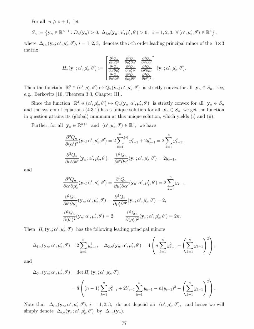
For all n > s+ 1, let
Sn :=yn ∈ R
n+1 : Dn(yn) > 0, ∆i,n(yn;α′, µ′
ε, θ′) > 0, i = 1, 2, 3, ∀ (α′, µ′
ε, θ′) ∈ R
3,
where ∆i,n(yn;α′, µ′
ε, θ′), i = 1, 2, 3, denotes the i-th order leading principal minor of the 3×3
matrix
Hn(yn;α′, µ′
ε, θ′) :=
∂2Qn
∂(α′)2∂2Qn
∂µ′ε∂α
′
∂2Qn
∂θ′∂α′
∂2Qn
∂α′∂µ′ε
∂2Qn
∂(µ′ε)
2∂2Qn
∂θ′∂µε
∂2Qn
∂α′∂θ′∂2Qn
∂µ′ε∂θ
′
∂2Qn
∂(θ′)2
(yn;α
′, µ′ε, θ
′).
Then the function R3 ∋ (α′, µ′ε, θ
′) 7→ Qn(yn;α′, µ′
ε, θ′) is strictly convex for all yn ∈ Sn, see,
e.g., Berkovitz [10, Theorem 3.3, Chapter III].
Since the function R3 ∋ (α′, µ′ε, θ
′) 7→ Qn(yn;α′, µ′
ε, θ′) is strictly convex for all yn ∈ Sn
and the system of equations (4.3.1) has a unique solution for all yn ∈ Sn, we get the function
in question attains its (global) minimum at this unique solution, which yields (i) and (ii).
Further, for all yn ∈ Rn+1 and (α′, µ′ε, θ
′) ∈ R3, we have
∂2Qn
∂(α′)2(yn;α
′, µ′ε, θ
′) = 2
n∑(s)
k=1
y2k−1 + 2y2s−1 = 2
n∑
k=1
y2k−1,
∂2Qn
∂α′∂θ′(yn;α
′, µ′ε, θ
′) =∂2Qn
∂θ′∂α′ (yn;α′, µ′
ε, θ′) = 2ys−1,
and
∂2Qn
∂α′∂µ′ε
(yn;α′, µ′
ε, θ′) =
∂2Qn
∂µ′ε∂α
′ (yn;α′, µ′
ε, θ′) = 2
n∑
k=1
yk−1,
∂2Qn
∂θ′∂µ′ε
(yn;α′, µ′
ε, θ′) =
∂2Qn
∂µ′ε∂θ
′ (yn;α′, µ′
ε, θ′) = 2,
∂2Qn
∂(θ′)2(yn;α
′, µ′ε, θ
′) = 2,∂2Qn
∂(µ′ε)
2(yn;α
′, µ′ε, θ
′) = 2n.
Then Hn(yn;α′, µ′
ε, θ′) has the following leading principal minors
∆1,n(yn;α′, µ′
ε, θ′) = 2
n∑
k=1
y2k−1, ∆2,n(yn;α′, µ′
ε, θ′) = 4
n
n∑
k=1
y2k−1 −(
n∑
k=1
yk−1
)2 ,
and
∆3,n(yn;α′, µ′
ε, θ′) = detHn(yn;α
′, µ′ε, θ
′)
= 8
(n− 1)
n∑
k=1
y2k−1 + 2Ys−1
n∑
k=1
yk−1 − n(ys−1)2 −
(n∑
k=1
yk−1
)2 .
Note that ∆i,n(yn;α′, µ′
ε, θ′), i = 1, 2, 3, do not depend on (α′, µ′
ε, θ′), and hence we will
simply denote ∆i,n(yn;α′, µ′
ε, θ′) by ∆i,n(yn).
77
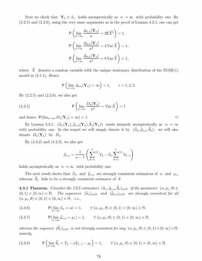
Next we check that Yn ∈ Sn holds asymptotically as n → ∞ with probability one. By
(2.2.5) and (2.2.6), using the very same arguments as in the proof of Lemma 4.2.1, one can get
P
(limn→∞
∆1,n(Yn)
n= 2EX2
)= 1,
P
(limn→∞
∆2,n(Yn)
n2= 4Var X
)= 1,
P
(limn→∞
∆3,n(Yn)
n2= 8Var X
)= 1,
where X denotes a random variable with the unique stationary distribution of the INAR(1)
model in (2.1.1). Hence
P(limn→∞
∆i,n(Yn) = ∞)= 1, i = 1, 2, 3.
By (2.2.5) and (2.2.6), we also get
P
(limn→∞
Dn(Yn)
n2= Var X
)= 1(4.3.5)
and hence P(limn→∞Dn(Yn) = ∞) = 1. 2
By Lemma 4.3.1, (αn(Yn), µε,n(Yn), θn(Yn)) exists uniquely asymptotically as n → ∞with probability one. In the sequel we will simply denote it by (αn, µε,n, θn), we will also
denote Dn(Yn) by Dn.
By (4.3.2) and (4.3.3), we also get
µε,n =1
n− 1
( n∑(s)
k=1
Yk − αn
n∑(s)
k=1
Yk−1
)
holds asymptotically as n → ∞ with probability one.
The next result shows that αn and µε,n are strongly consistent estimators of α and µε,
whereas θn fails to be a strongly consistent estimator of θ.
4.3.1 Theorem. Consider the CLS estimators (αn, µε,n, θn)n∈N of the parameter (α, µε, θ) ∈(0, 1) × (0,∞) × N. The sequences (αn)n∈N and (µε,n)n∈N are strongly consistent for all
(α, µε, θ) ∈ (0, 1)× (0,∞)× N, i.e.,
P( limn→∞
αn = α) = 1, ∀ (α, µε, θ) ∈ (0, 1)× (0,∞)× N,(4.3.6)
P( limn→∞
µε,n = µε) = 1, ∀ (α, µε, θ) ∈ (0, 1)× (0,∞)× N,(4.3.7)
whereas the sequence (θn)n∈N is not strongly consistent for any (α, µε, θ) ∈ (0, 1)×(0,∞)×N,
namely,
P(limn→∞
θn = Ys − αYs−1 − µε
)= 1, ∀ (α, µε, θ) ∈ (0, 1)× (0,∞)× N.(4.3.8)
78
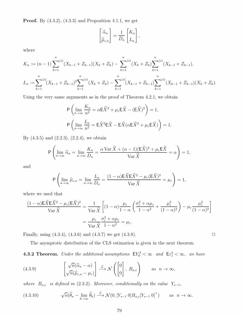
Proof. By (4.3.2), (4.3.3) and Proposition 4.1.1, we get
[αn
µε,n
]=
1
Dn
[Kn
Ln
],
where
Kn := (n− 1)
n∑(s)
k=1
(Xk−1 + Zk−1)(Xk + Zk)−n∑(s)
k=1
(Xk + Zk)
n∑(s)
k=1
(Xk−1 + Zk−1),
Ln :=
n∑(s)
k=1
(Xk−1 + Zk−1)2
n∑(s)
k=1
(Xk + Zk)−n∑(s)
k=1
(Xk−1 + Zk−1)
n∑(s)
k=1
(Xk−1 + Zk−1)(Xk + Zk).
Using the very same arguments as in the proof of Theorem 4.2.1, we obtain
P
(limn→∞
Kn
n2= αEX2 + µεEX − (EX)2
)= 1,
P
(limn→∞
Ln
n2= EX2EX − EX(αEX2 + µεEX)
)= 1.
By (4.3.5) and (2.2.3), (2.2.4), we obtain
P
(limn→∞
αn = limn→∞
Kn
Dn
=αVar X + (α− 1)(EX)2 + µεEX
Var X= α
)= 1,
and
P
(limn→∞
µε,n = limn→∞
Ln
Dn
=(1− α)EXEX2 − µε(EX)2
Var X= µε
)= 1,
where we used that
(1− α)EXEX2 − µε(EX)2
Var X=
1
Var X
[(1− α)
µε
1− α
(σ2ε + αµε
1− α2+
µ2ε
(1− α)2
)− µε
µ2ε
(1− α)2
]
=µε
Var X
σ2ε + αµε
1− α2= µε.
Finally, using (4.3.4), (4.3.6) and (4.3.7) we get (4.3.8). 2
The asymptotic distribution of the CLS estimation is given in the next theorem.
4.3.2 Theorem. Under the additional assumptions EY 30 < ∞ and Eε31 < ∞, we have
[ √n(αn − α)
√n(µε,n − µε)
]L−→ N
([0
0
], Bα,ε
)as n → ∞,(4.3.9)
where Bα,ε is defined in (2.3.2). Moreover, conditionally on the value Ys−1,
√n(θn − lim
k→∞θk)
L−→ N (0, [Ys−1 0]Bα,ε[Ys−1 0]⊤) as n → ∞.(4.3.10)
79
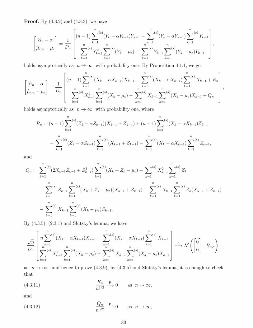
Proof. By (4.3.2) and (4.3.3), we have
[αn − α
µε,n − µε
]=
1
Dn
(n− 1)
n∑(s)
k=1
(Yk − αYk−1)Yk−1 −n∑(s)
k=1
(Yk − αYk−1)
n∑(s)
k=1
Yk−1
n∑(s)
k=1
Y 2k−1
n∑(s)
k=1
(Yk − µε)−n∑(s)
k=1
Yk−1
n∑(s)
k=1
(Yk − µε)Yk−1
,
holds asymptotically as n → ∞ with probability one. By Proposition 4.1.1, we get
[αn − α
µε,n − µε
]=
1
Dn
(n− 1)
n∑(s)
k=1
(Xk − αXk−1)Xk−1 −n∑(s)
k=1
(Xk − αXk−1)
n∑(s)
k=1
Xk−1 +Rn
n∑(s)
k=1
X2k−1
n∑(s)
k=1
(Xk − µε)−n∑(s)
k=1
Xk−1
n∑(s)
k=1
(Xk − µε)Xk−1 +Qn
,
holds asymptotically as n → ∞ with probability one, where
Rn :=(n− 1)
n∑(s)
k=1
(Zk − αZk−1)(Xk−1 + Zk−1) + (n− 1)
n∑(s)
k=1
(Xk − αXk−1)Zk−1
−n∑(s)
k=1
(Zk − αZk−1)
n∑(s)
k=1
(Xk−1 + Zk−1)−n∑(s)
k=1
(Xk − αXk−1)
n∑(s)
k=1
Zk−1,
and
Qn :=
n∑(s)
k=1
(2Xk−1Zk−1 + Z2k−1)
n∑(s)
k=1
(Xk + Zk − µε) +
n∑(s)
k=1
X2k−1
n∑(s)
k=1
Zk
−n∑(s)
k=1
Zk−1
n∑(s)
k=1
(Xk + Zk − µε)(Xk−1 + Zk−1)−n∑(s)
k=1
Xk−1
n∑(s)
k=1
Zk(Xk−1 + Zk−1)
−n∑(s)
k=1
Xk−1
n∑(s)
k=1
(Xk − µε)Zk−1.
By (4.3.5), (2.3.1) and Slutsky’s lemma, we have
√n
Dn
n
n∑(s)
k=1
(Xk − αXk−1)Xk−1 −n∑(s)
k=1
(Xk − αXk−1)
n∑(s)
k=1
Xk−1
n∑(s)
k=1
X2k−1
n∑(s)
k=1
(Xk − µε)−n∑(s)
k=1
Xk−1
n∑(s)
k=1
(Xk − µε)Xk−1
L−→ N([
0
0
], Bα,ε
),
as n → ∞, and hence to prove (4.3.9), by (4.3.5) and Slutsky’s lemma, it is enough to check
that
Rn
n3/2
P−→ 0 as n → ∞,(4.3.11)
and
Qn
n3/2
P−→ 0 as n → ∞,(4.3.12)
80
whereP−→ denotes convergence in probability. By (4.2.15) and (4.2.16), to prove (4.3.11) it
remains to check that
1√n
n∑(s)
k=1
(Xk − αXk−1)Zk−1P−→ 0 as n → ∞,(4.3.13)
1√n
n∑(s)
k=1
(Zk − αZk−1) ·1
n
n∑(s)
k=1
(Xk−1 + Zk−1)P−→ 0 as n → ∞,(4.3.14)
1
n
n∑(s)
k=1
(Xk − αXk−1) ·1√n
n∑(s)
k=1
Zk−1P−→ 0 as n → ∞.(4.3.15)
Using (4.2.14) and that
1√n
n∑(s)
k=1
(Xk − αXk−1)Zk−1 =1√n
n∑(s)
k=1
(Xk − αXk−1 − µε)Zk−1 + µε1√n
n∑(s)
k=1
Zk−1,
to prove (4.3.13), it is enough to check that
1√n
n∑(s)
k=1
Zk−1P−→ 0 as n → ∞.(4.3.16)
Using that Zk > 0, k ∈ N, by Markov’s inequality, it is enough to check that
limn→∞
1√n
n∑(s)
k=1
EZk−1 = 0.(4.3.17)
Since, by (4.1.4), EZs+k = θαk, k > 0, we have
1√n
n∑(s)
k=1
EZk−1 6θ√n
n∑
k=0
αk =θ√n
αn+1 − 1
α− 1→ 0 as n → ∞.(4.3.18)
Using that
P
(limn→∞
1
n
n∑(s)
k=1
(Xk−1 + Zk−1) = EX
)= 1,
to prove (4.3.14) it is enough to check that
1√n
n∑(s)
k=1
(Zk − αZk−1)L1−→ 0 as n → ∞.(4.3.19)
To verify (4.3.19) it is enough to show that
limn→∞
1√n
n∑(s)
k=1
E(Zk − αZk−1) = 0,(4.3.20)
limn→∞
1
nE
( n∑(s)
k=1
(Zk − αZk−1)
)2
= 0.(4.3.21)
81
Using that EZk = αEZk−1, k > s + 1, we get (4.3.20) is satisfied. Using that E[(Zk −αZk−1)(Zℓ − αZℓ−1)] = 0 for all k 6= ℓ, k, ℓ > s+ 1, we have
1
nE
( n∑(s)
k=1
(Zk − αZk−1)
)2
=1
n
n∑(s)
k=1
E(Zk − αZk−1)2 → 0 as n → ∞,
as we showed in the proof of Theorem 4.2.2. Using that
P
(limn→∞
1
n
n∑(s)
k=1
(Xk − αXk−1) = (1− α)EX
)= 1,
to prove (4.3.15) it is enough to verify (4.3.16) which was already done.
Now we turn to prove (4.3.12). Using (4.3.16) and that
P
(limn→∞
1
n
n∑(s)
k=1
(Xk + Zk − µε) = EX − µε
)= 1,
P
(limn→∞
1
n
n∑(s)
k=1
X2k−1 = EX2
)= 1,
P
(limn→∞
1
n
n∑(s)
k=1
(Xk + Zk − µε)(Xk−1 + Zk−1) = αEX2 + µεEX − µεEX = αEX2
)= 1,
it is enough to verify that
1√n
n∑(s)
k=1
Xk−1Zk−1P−→ 0 as n → ∞,(4.3.22)
1√n
n∑(s)
k=1
Z2k−1
P−→ 0 as n → ∞,(4.3.23)
1√n
n∑(s)
k=1
Zk−1ZkP−→ 0 as n → ∞.(4.3.24)
To prove (4.3.22), using that the processes X and Z are non-negative, by Markov’s inequality,
it is enough to verify that
limn→∞
1√n
n∑(s)
k=1
E(Xk−1Zk−1) = 0.
Using that the processes X and Z are independent and limk→∞ EXk−1 = EX , as in the
proof of (4.2.15), we get it is enough to check that
limn→∞
1√n
n∑(s)
k=1
EZk−1 = 0,
which follows by (4.3.18). Similarly, to prove (4.3.23), it is enough to show that
limn→∞
1√n
n∑(s)
k=1
EZ2k−1 = 0.
82
By (4.1.5), we have for all n > s+ 1,
1√n
n∑(s)
k=1
EZ2k−1 6
1√n
n∑
k=0
(θ2α2k − θαk(αk − 1)) 6θ2√n
α2(n+1) − 1
α2 − 1+
θ√n
αn+1 − 1
α− 1→ 0,
as n → ∞. Similarly, to prove (4.3.24), it is enough to check that
limn→∞
1√n
n∑(s)
k=1
E(Zk−1Zk) = 0.
By (4.1.6), we have for all n > s+ 1,
1√n
n∑(s)
k=1
E(Zk−1Zk) 61√n
n∑
k=1
(θ2α2k−1 + θαk(1− αk)) 6θ2
α√n
α2n − 1
α2 − 1+
θ√n
αn − 1
α− 1→ 0,
as n → ∞.
Finally, using (4.3.4) and (4.3.8), we get
√n(θn − lim
k→∞θk) = −√
n(αn − α)Ys−1 −√n(µε,n − µε) =
[−Ys−1 −1
] [ √n(αn − α)
√n(µε,n − µε)
],
and hence, by (4.3.9), we have (4.3.10). 2
4.4 Two outliers, estimation of the mean of the offspring distribu-
tion and the outliers’ sizes
We assume that I = 2 and that the relevant time points s1, s2 ∈ N, s1 6= s2, are known.
We concentrate on the CLS estimation of (α, θ1, θ2). We have
E(Yk | FYk−1) = αYk−1 + µε + δk,s1θ1 + δk,s2θ2, k ∈ N.
Hence for all n > max(s1, s2),
n∑
k=1
(Yk − E(Yk | FY
k−1))2
=
n∑
k=1
(s1,s2)(Yk − αYk−1 − µε
)2+(Ys1 − αYs1−1 − µε − θ1
)2+(Ys2 − αYs2−1 − µε − θ2
)2.
For all n > max(s1, s2), n ∈ N, we define the function Qn : Rn+1 × R3 → R, as
Qn(yn;α′, θ′1, θ
′2)
:=n∑
k=1
(s1,s2)(yk − α′yk−1 − µε
)2+(ys1 − α′ys1−1 − µε − θ′1
)2+(ys2 − α′ys2−1 − µε − θ′2
)2,
83
for all yn ∈ Rn+1, α′, θ′1, θ
′2 ∈ R. By definition, for all n > max(s1, s2), a CLS estimator for
the parameter (α, θ1, θ2) ∈ (0, 1)×N2 is a measurable function (αn, θ1,n, θ2,n) : Sn → R3 such
that
Qn(yn; αn(yn), θ1,n(yn), θ2,n(yn)) = inf(α′,θ′1,θ
′2)∈R3
Qn(yn;α′, θ′1, θ
′2) ∀ yn ∈ Sn,
where Sn is suitable subset of Rn+1 (defined in the proof of Lemma 4.4.1). We note that we
do not define the CLS estimator (αn, θ1,n, θ2,n) for all samples yn ∈ Rn+1. For all yn ∈ R
n+1,
α′, θ′1, θ′2 ∈ R,
∂Qn
∂α′ (yn;α′, θ′1, θ
′2) =
n∑
k=1
(s1,s2)
(−2)(yk − α′yk−1 − µε
)yk−1 − 2
(ys1 − α′ys1−1 − µε − θ′1
)ys1−1
− 2(ys2 − α′ys2−1 − µε − θ′2
)ys2−1,
∂Qn
∂θ′1(yn;α
′, θ′1, θ′2) = −2
(ys1 − α′ys1−1 − µε − θ′1
),
∂Qn
∂θ′2(yn;α
′, θ′1, θ′2) = −2
(ys2 − α′ys2−1 − µε − θ′2
).
The next lemma is about the existence and uniqueness of the CLS estimator of (α, θ1, θ2).
4.4.1 Lemma. There exist subsets Sn ⊂ Rn+1, n > max(3, s1, s2) with the following proper-
ties:
(i) there exists a unique CLS estimator (αn, θ1,n, θ2,n) : Sn → R3,
(ii) for all yn ∈ Sn, the system of equations
∂Qn
∂α′ (yn;α′, θ′1, θ
′2) = 0,
∂Qn
∂θ′1(yn;α
′, θ′1, θ′2) = 0,
∂Qn
∂θ′2(yn;α
′, θ′1, θ′2) = 0,
(4.4.1)
has the unique solution
αn(yn) =
n∑
k=1
(s1,s2)
(yk − µε)yk−1
n∑
k=1
(s1,s2)
y2k−1
,(4.4.2)
θi,n(yn) = ysi − αn(yn)ysi−1 − µε, i = 1, 2,(4.4.3)
(iii) Yn ∈ Sn holds asymptotically as n → ∞ with probability one.
84
Proof. One can easily check that the unique solution of the system of equations (4.4.1) takes
the form (4.4.2) and (4.4.3) whenevern∑
k=1
(s1,s2)
y2k−1 > 0.
For all n > max(3, s1, s2), let
Sn :=yn ∈ R
n+1 : ∆i,n(yn;α′, θ′1, θ
′2) > 0, i = 1, 2, 3, ∀ (α′, θ′1, θ
′2) ∈ R
3,
where ∆i,n(yn;α′, µ′
ε, θ′), i = 1, 2, 3, denotes the i-th order leading principal minor of the 3×3
matrix
Hn(yn;α′, θ′1, θ
′2) :=
∂2Qn
∂(α′)2∂2Qn
∂θ′1∂α′
∂2Qn
∂θ′2∂α′
∂2Qn
∂α′∂θ′1
∂2Qn
∂(θ′1)2
∂2Qn
∂θ′2∂θ′1
∂2Qn
∂α′∂θ′2
∂2Qn
∂θ′1∂θ′2
∂2Qn
∂(θ′2)2
(yn;α
′, θ′1, θ′2)
Then the function R3 ∋ (α′, θ′1, θ′2) 7→ Qn(yn;α
′, θ′1, θ′2) is strictly convex for all yn ∈ Sn, see,
e.g., Berkovitz [10, Theorem 3.3, Chapter III]. Further, for all yn ∈ Rn+1 and (α′, θ′1, θ′2) ∈ R3,
we have
∂2Qn
∂(α′)2(yn;α
′, θ′1, θ′2) = 2
n∑(s1,s2)
k=1
y2k−1 + 2y2s1−1 + 2y2s2−1 = 2n∑
k=1
y2k−1,
∂2Qn
∂α′∂θ′1(yn;α
′, θ′1, θ′2) =
∂2Qn
∂θ′1∂α′ (yn;α
′, θ′1, θ′2) = 2ys1−1,
∂2Qn
∂α′∂θ′2(yn;α
′, θ′1, θ′2) =
∂2Qn
∂θ′2∂α′ (yn;α
′, θ′1, θ′2) = 2ys2−1,
∂2Qn
∂θ′1∂θ′2
(yn;α′, θ′1, θ
′2) =
∂2Qn
∂θ′2∂θ′1
(yn;α′, θ′1, θ
′2) = 0,
∂2Qn
∂(θ′1)2(yn;α
′, θ′1, θ′2) = 2,
∂2Qn
∂(θ′2)2(yn;α
′, θ′1, θ′2) = 2.
This yields that the system of equations (4.4.1) has a unique solution for all yn ∈ Sn. Using
also that the function R3 ∋ (α′, θ′1, θ′2) 7→ Qn(yn;α
′, θ′1, θ′2) is strictly convex for all yn ∈ Sn,
we get the function in question attains its (global) minimum at this unique solution, which
yields (i) and (ii).
Then Hn(yn;α′, θ′1, θ
′2) has the following leading principal minors
∆1,n(yn;α′, θ′1, θ
′2) = 2
n∑
k=1
y2k−1, ∆2,n(yn;α′, θ′1, θ
′2) = 4
(n∑
k=1
y2k−1 − (ys1−1)2
),
and
∆3,n(yn;α′, θ′1, θ
′2) = detHn(yn;α
′, θ′1, θ′2) = 8
(n∑
k=1
y2k−1 − (ys1−1)2 − (ys2−1)
2
).
Note that ∆i,n(yn;α′, θ′1, θ
′2), i = 1, 2, 3, do not depend on (α′, θ′1, θ
′2), and hence we will
simply denote ∆i,n(yn;α′, θ′1, θ
′2) by ∆i,n(yn).
85
Next we check that Yn ∈ Sn holds asymptotically as n → ∞ with probability one. By
(2.2.5) and (2.2.6), using the very same arguments as in the proof of Lemma 4.2.1, one can get
P
(limn→∞
∆1,n(Yn)
n= 2EX2
)= 1,
P
(limn→∞
∆2,n(Yn)
n= 4EX2
)= 1,
P
(limn→∞
∆3,n(Yn)
n= 8EX2
)= 1,
where X denotes a random variable with the unique stationary distribution of the INAR(1)
model in (2.1.1). Hence
P(limn→∞
∆i,n(Yn) = ∞)= 1, i = 1, 2, 3,
which yields that Yn ∈ Sn holds asymptotically as n → ∞ with probability one. 2
By Lemma 4.4.1, (αn(Yn), θ1,n(Yn), θ2,n(Yn)) exists uniquely asymptotically as n → ∞with probability one. In the sequel we will simply denote it by (αn, θ1,n, θ2,n).
The next result shows that αn is a strongly consistent estimator of α, whereas θi,n,
i = 1, 2, fail to be strongly consistent estimators of θi,n, i = 1, 2, respectively.
4.4.1 Theorem. Consider the CLS estimators (αn, θ1,n, θ2,n)n∈N of the parameter (α, θ1, θ2) ∈(0, 1)×N2. The sequence (αn)n∈N is strongly consistent for all (α, θ1, θ2) ∈ (0, 1)×N2, i.e.,
P( limn→∞
αn = α) = 1, ∀ (α, θ1, θ2) ∈ (0, 1)× N2,(4.4.4)
whereas the sequences (θ1,n)n∈N and (θ2,n)n∈N are not strongly consistent for any (α, θ1, θ2) ∈(0, 1)× N2, namely,
P(limn→∞
θi,n = Ysi − αYsi−1 − µε
)= 1, ∀ (α, θ1, θ1) ∈ (0, 1)× N
2, i = 1, 2.(4.4.5)
Proof. By (4.4.2) and Proposition 4.1.2, we get
αn =
n∑(s1,s2)
k=1
(Xk − µε)Xk−1 +Kn
n∑(s1,s2)
k=1
X2k−1 + Ln
,
holds asymptotically as n → ∞ with probability one, where
Kn :=
n∑(s1,s2)
k=1
(Z(1)k + Z
(2)k )(Xk−1 + Z
(1)k−1 + Z
(2)k−1) +
n∑(s1,s2)
k=1
(Xk − µε)(Z(1)k−1 + Z
(2)k−1),
Ln :=
n∑(s1,s2)
k=1
[(Z
(1)k−1)
2 + (Z(2)k−1)
2 + 2Xk−1Z(1)k−1 + 2Xk−1Z
(2)k−1 + 2Z
(1)k−1Z
(2)k−1
].
86
Using the very same arguments as in the proof of Theorem 4.2.1, one can obtain
P
(limn→∞
Kn
n= 0
)= 1 and P
(limn→∞
Ln
n= 0
)= 1.
Indeed, the only fact that was not verified in the proof of Theorem 4.2.1 is that
P
(limn→∞
1
n
n∑(s1,s2)
k=1
Z(1)k Z
(2)k = 0
)= 1.(4.4.6)
By Cauchy-Schwartz’s inequality and Proposition 4.1.2,
1
n
n∑(s1,s2)
k=1
Z(1)k Z
(2)k 6
√√√√ 1
n
n∑
k=1
(Z(1)k )2
1
n
n∑
k=1
(Z(2)k )2 → 0 as n → ∞,
with probability one.
Finally, by (4.4.3) and (4.4.4), we have (4.4.5). 2
4.4.1 Remark. Since[Ys1 − αYs1−1 − µε
Ys2 − αYs2−1 − µε
]=
[Xs1 − αXs1−1 − µε + θ1
Xs2 − αXs2−1 − µε + θ2
],
and
Cov(Xs1 − αXs1−1 − µε + θ1, Xs2 − αXs2−1 − µε + θ2)
= E[(Xs1 − αXs1−1 − µε)(Xs2 − αXs2−1 − µε)
]
= E
Xs1−1∑
j=1
(ξs1,j − α) + (εs1 − µε)
Xs2−1∑
j=1
(ξs2,j − α) + (εs2 − µε)
= 0,
by Remark 4.2.1, we get
Var
[Ys1 − αYs1−1 − µε
Ys2 − αYs2−1 − µε
]
=
[αs1(1− α)EY0 + αµε(1− αs1−1) + σ2
ε 0
0 αs2(1− α)EY0 + αµε(1− αs2−1) + σ2ε
].
2
The asymptotic distribution of the CLS estimation is given in the next theorem.
4.4.2 Theorem. Under the additional assumptions EY 30 < ∞ and Eε31 < ∞, we have
√n(αn − α)
L−→ N (0, σ2α,ε) as n → ∞,(4.4.7)
where σ2α, ε is defined in (2.2.9). Moreover, conditionally on the values Ys1−1 and Ys2−1,
[√n(θ1,n − limk→∞ θ1,k
)√n(θ2,n − limk→∞ θ2,k
)]
L−→ N([
0
0
], σ2
α,ε
[Y 2s1−1 Ys1−1Ys2−1
Ys1−1Ys2−1 Y 2s2−1
])as n → ∞.
(4.4.8)
87
Proof. By (4.4.2), we get
αn − α =
n∑(s1,s2)
k=1
(Yk − αYk−1 − µε)Yk−1
n∑(s1,s2)
k=1
Y 2k−1
,
holds asymptotically as n → ∞ with probability one. To prove (4.4.7), using Proposition
4.1.2 and (4.2.14)–(4.2.18), it is enough to check that
1√n
n∑
k=1
(Z(1)k − αZ
(1)k−1)Z
(2)k−1
P−→ 0 as n → ∞,(4.4.9)
1√n
n∑
k=1
(Z(2)k − αZ
(2)k−1)Z
(1)k−1
P−→ 0 as n → ∞.(4.4.10)
To prove (4.4.9) it is enough to verify that
limn→∞
1√n
n∑
k=1
E[(Z(1)k − αZ
(1)k−1)Z
(2)k−1] = 0,(4.4.11)
limn→∞
1
nE
(n∑
k=1
(Z(1)k − αZ
(1)k−1)Z
(2)k−1
)2
= 0.(4.4.12)
Since the processes Z(1) and Z(2) are independent, we have
E[(Z(1)k − αZ
(1)k−1)Z
(2)k−1] = E(Z
(1)k − αZ
(1)k−1)EZ
(2)k−1 = 0, k ∈ N,
which yields (4.4.11). Using that for all k, ℓ ∈ N, k > ℓ,
E[(Z
(1)k − αZ
(1)k−1)Z
(2)k−1(Z
(1)ℓ − αZ
(1)ℓ−1)Z
(2)ℓ−1
]= E
[(Z
(1)k − αZ
(1)k−1)(Z
(1)ℓ − αZ
(1)ℓ−1)
]E(Z
(2)k−1Z
(2)ℓ−1)
= E[(Z
(1)ℓ − αZ
(1)ℓ−1)E(Z
(1)k − αZ
(1)k−1 | FZ(1)
k−1 )]E(Z
(2)k−1Z
(2)ℓ−1)
= 0 · E(Z(2)k−1Z
(2)ℓ−1) = 0,
we get
1
nE
(n∑
k=1
(Z(1)k − αZ
(1)k−1)Z
(2)k−1
)2
=1
n
n∑
k=1
E[(Z(1)k − αZ
(1)k−1)
2(Z(2)k−1)
2]
=1
n
n∑
k=1
E(Z(1)k − αZ
(1)k−1)
2E(Z(2)k−1)
2
62
n
n∑
k=1
E((Z(1)k )2 + α2(Z
(1)k−1)
2)E(Z(2)k−1)
2.
88

Hence, by (4.1.5),
1
nE
(n∑
k=1
(Z(1)k − αZ
(1)k−1)Z
(2)k−1
)2
62
n
n∑
k=0
[(θ21α
2k + θ1αk(1− αk) + α2θ21α
2(k−1) + α2θ1αk−1(1− αk−1)
)
×(θ22α
2(k−1) + θ2αk−1(1− αk−1)
)]
62(θ21 + θ1)
n
(θ22α2n − 1
α2 − 1+ θ2
αn − 1
α− 1+ θ22
α2n − 1
α2 − 1+ αθ2
αn − 1
α− 1
)→ 0 as n → ∞.
Similarly one can check (4.4.10).
Moreover, conditionally on the values Ys1−1 and Ys2−1, by (4.4.3), (4.4.5) and (4.4.7),
[√n(θ1,n − limk→∞ θ1,k
)√n(θ2,n − limk→∞ θ2,k
)]=
√n
[θ1,n − (Ys1 − αYs1−1 − µε)
θ2,n − (Ys2 − αYs2−1 − µε)
]=
√n
[−(αn − α)Ys1−1
−(αn − α)Ys2−1
]
L−→ N([
0
0
], σ2
α, ε
[Y 2s1−1 Ys1−1Ys2−1
Ys1−1Ys2−1 Y 2s2−1
])as n → ∞.
2
4.5 Two outliers, estimation of the mean of the offspring and inno-
vation distributions and the outliers’ sizes
We assume that I = 2 and that the relevant time points s1, s2 ∈ N, s1 6= s2, are known.
We concentrate on the CLS estimation of (α, µε, θ1, θ2). We have
E(Yk | FYk−1) = αYk−1 + µε + δk,s1θ1 + δk,s2θ2, k ∈ N.
Hence for all n > max(s1, s2), n ∈ N,
n∑
k=1
(Yk − E(Yk | FY
k−1))2
=
n∑
k=1
(s1,s2)(Yk − αYk−1 − µε
)2+(Ys1 − αYs1−1 − µε − θ1
)2+(Ys2 − αYs2−1 − µε − θ2
)2.
For all n > max(s1, s2), n ∈ N, we define the function Qn : Rn+1 × R4 → R, as
Qn(yn;α′, µ′
ε, θ′1, θ
′2)
:=
n∑
k=1
(s1,s2)(yk − α′yk−1 − µ′
ε
)2+(ys1 − α′ys1−1 − µ′
ε − θ′1)2
+(ys2 − α′ys2−1 − µ′
ε − θ′2)2,
89
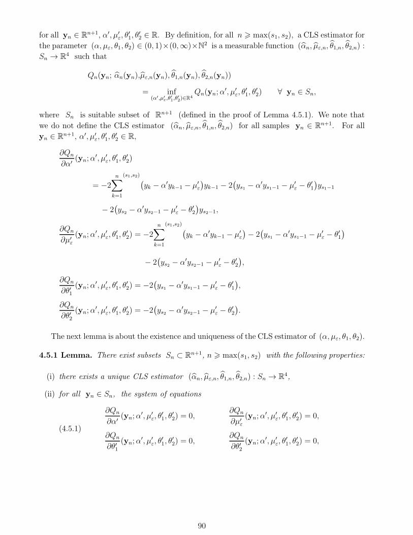
for all yn ∈ Rn+1, α′, µ′
ε, θ′1, θ
′2 ∈ R. By definition, for all n > max(s1, s2), a CLS estimator for
the parameter (α, µε, θ1, θ2) ∈ (0, 1)×(0,∞)×N2 is a measurable function (αn, µε,n, θ1,n, θ2,n) :
Sn → R4 such that
Qn(yn; αn(yn),µε,n(yn), θ1,n(yn), θ2,n(yn))
= inf(α′,µ′
ε,θ′1,θ
′2)∈R4
Qn(yn;α′, µ′
ε, θ′1, θ
′2) ∀ yn ∈ Sn,
where Sn is suitable subset of Rn+1 (defined in the proof of Lemma 4.5.1). We note that
we do not define the CLS estimator (αn, µε,n, θ1,n, θ2,n) for all samples yn ∈ Rn+1. For all
yn ∈ Rn+1, α′, µ′ε, θ
′1, θ
′2 ∈ R,
∂Qn
∂α′ (yn;α′, µ′
ε, θ′1, θ
′2)
= −2n∑
k=1
(s1,s2)(yk − α′yk−1 − µ′
ε
)yk−1 − 2
(ys1 − α′ys1−1 − µ′
ε − θ′1)ys1−1
− 2(ys2 − α′ys2−1 − µ′
ε − θ′2)ys2−1,
∂Qn
∂µ′ε
(yn;α′, µ′
ε, θ′1, θ
′2) = −2
n∑
k=1
(s1,s2)(yk − α′yk−1 − µ′
ε
)− 2(ys1 − α′ys1−1 − µ′
ε − θ′1)
− 2(ys2 − α′ys2−1 − µ′
ε − θ′2),
∂Qn
∂θ′1(yn;α
′, µ′ε, θ
′1, θ
′2) = −2
(ys1 − α′ys1−1 − µ′
ε − θ′1),
∂Qn
∂θ′2(yn;α
′, µ′ε, θ
′1, θ
′2) = −2
(ys2 − α′ys2−1 − µ′
ε − θ′2).
The next lemma is about the existence and uniqueness of the CLS estimator of (α, µε, θ1, θ2).
4.5.1 Lemma. There exist subsets Sn ⊂ Rn+1, n > max(s1, s2) with the following properties:
(i) there exists a unique CLS estimator (αn, µε,n, θ1,n, θ2,n) : Sn → R4,
(ii) for all yn ∈ Sn, the system of equations
∂Qn
∂α′ (yn;α′, µ′
ε, θ′1, θ
′2) = 0,
∂Qn
∂µ′ε
(yn;α′, µ′
ε, θ′1, θ
′2) = 0,
∂Qn
∂θ′1(yn;α
′, µ′ε, θ
′1, θ
′2) = 0,
∂Qn
∂θ′2(yn;α
′, µ′ε, θ
′1, θ
′2) = 0,
(4.5.1)
90
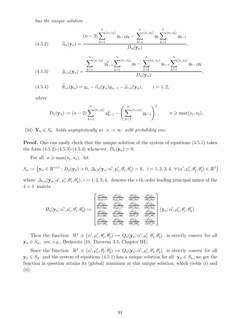
has the unique solution
αn(yn) =
(n− 2)
n∑(s1,s2)
k=1
yk−1yk −n∑(s1,s2)
k=1
yk
n∑(s1,s2)
k=1
yk−1
Dn(yn),(4.5.2)
µε,n(yn) =
n∑(s1,s2)
k=1
y2k−1
n∑(s1,s2)
k=1
yk −n∑(s1,s2)
k=1
yk−1
n∑(s1,s2)
k=1
yk−1yk
Dn(yn),(4.5.3)
θi,n(yn) = ysi − αn(yn)ysi−1 − µε,n(yn), i = 1, 2,(4.5.4)
where
Dn(yn) := (n− 2)
n∑(s1,s2)
k=1
y2k−1 −( n∑(s1,s2)
k=1
yk−1
)2
, n > max(s1, s2),
(iii) Yn ∈ Sn holds asymptotically as n → ∞ with probability one.
Proof. One can easily check that the unique solution of the system of equations (4.5.1) takes
the form (4.5.2)-(4.5.3)-(4.5.4) whenever Dn(yn) > 0.
For all n > max(s1, s2), let
Sn :=yn ∈ R
n+1 : Dn(yn) > 0, ∆i,n(yn;α′, µ′
ε, θ′1, θ
′2) > 0, i = 1, 2, 3, 4, ∀ (α′, µ′
ε, θ′1, θ
′2) ∈ R
4,
where ∆i,n(yn;α′, µ′
ε, θ′1, θ
′2), i = 1, 2, 3, 4, denotes the i-th order leading principal minor of the
4× 4 matrix
Hn(yn;α′, µ′
ε, θ′1, θ
′2) :=
∂2Qn
∂(α′)2∂2Qn
∂µ′ε∂α
′
∂2Qn
∂θ′1∂α′
∂2Qn
∂θ′2∂α′
∂2Qn
∂α′∂µ′ε
∂2Qn
∂(µ′ε)
2∂2Qn
∂θ′1∂µ′ε
∂2Qn
∂θ′2∂µ′ε
∂2Qn
∂α′∂θ′1
∂2Qn
∂µ′ε∂θ
′1
∂2Qn
∂(θ′1)2
∂2Qn
∂θ′2∂θ′1
∂2Qn
∂α′∂θ′2
∂2Qn
∂µ′ε∂θ
′2
∂2Qn
∂θ′1∂θ′2
∂2Qn
∂(θ′2)2
(yn;α
′, µ′ε, θ
′1, θ
′2).
Then the function R4 ∋ (α′, µ′ε, θ
′1, θ
′2) 7→ Qn(yn;α
′, µ′ε, θ
′1, θ
′2) is strictly convex for all
yn ∈ Sn, see, e.g., Berkovitz [10, Theorem 3.3, Chapter III].
Since the function R4 ∋ (α′, µ′ε, θ
′1, θ
′2) 7→ Qn(yn;α
′, µ′ε, θ
′1, θ
′2) is strictly convex for all
yn ∈ Sn and the system of equations (4.5.1) has a unique solution for all yn ∈ Sn, we get the
function in question attains its (global) minimum at this unique solution, which yields (i) and
(ii).
91
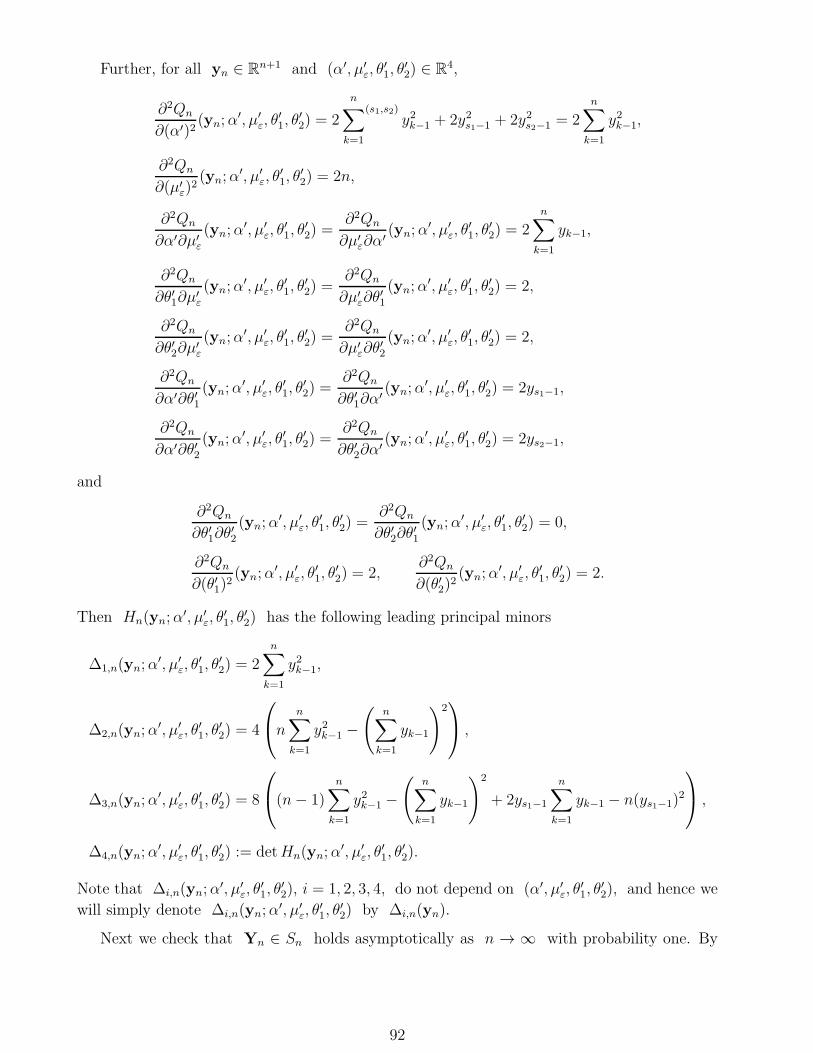
Further, for all yn ∈ Rn+1 and (α′, µ′
ε, θ′1, θ
′2) ∈ R
4,
∂2Qn
∂(α′)2(yn;α
′, µ′ε, θ
′1, θ
′2) = 2
n∑(s1,s2)
k=1
y2k−1 + 2y2s1−1 + 2y2s2−1 = 2
n∑
k=1
y2k−1,
∂2Qn
∂(µ′ε)
2(yn;α
′, µ′ε, θ
′1, θ
′2) = 2n,
∂2Qn
∂α′∂µ′ε
(yn;α′, µ′
ε, θ′1, θ
′2) =
∂2Qn
∂µ′ε∂α
′ (yn;α′, µ′
ε, θ′1, θ
′2) = 2
n∑
k=1
yk−1,
∂2Qn
∂θ′1∂µ′ε
(yn;α′, µ′
ε, θ′1, θ
′2) =
∂2Qn
∂µ′ε∂θ
′1
(yn;α′, µ′
ε, θ′1, θ
′2) = 2,
∂2Qn
∂θ′2∂µ′ε
(yn;α′, µ′
ε, θ′1, θ
′2) =
∂2Qn
∂µ′ε∂θ
′2
(yn;α′, µ′
ε, θ′1, θ
′2) = 2,
∂2Qn
∂α′∂θ′1(yn;α
′, µ′ε, θ
′1, θ
′2) =
∂2Qn
∂θ′1∂α′ (yn;α
′, µ′ε, θ
′1, θ
′2) = 2ys1−1,
∂2Qn
∂α′∂θ′2(yn;α
′, µ′ε, θ
′1, θ
′2) =
∂2Qn
∂θ′2∂α′ (yn;α
′, µ′ε, θ
′1, θ
′2) = 2ys2−1,
and
∂2Qn
∂θ′1∂θ′2
(yn;α′, µ′
ε, θ′1, θ
′2) =
∂2Qn
∂θ′2∂θ′1
(yn;α′, µ′
ε, θ′1, θ
′2) = 0,
∂2Qn
∂(θ′1)2(yn;α
′, µ′ε, θ
′1, θ
′2) = 2,
∂2Qn
∂(θ′2)2(yn;α
′, µ′ε, θ
′1, θ
′2) = 2.
Then Hn(yn;α′, µ′
ε, θ′1, θ
′2) has the following leading principal minors
∆1,n(yn;α′, µ′
ε, θ′1, θ
′2) = 2
n∑
k=1
y2k−1,
∆2,n(yn;α′, µ′
ε, θ′1, θ
′2) = 4
n
n∑
k=1
y2k−1 −(
n∑
k=1
yk−1
)2 ,
∆3,n(yn;α′, µ′
ε, θ′1, θ
′2) = 8
(n− 1)
n∑
k=1
y2k−1 −(
n∑
k=1
yk−1
)2
+ 2ys1−1
n∑
k=1
yk−1 − n(ys1−1)2
,
∆4,n(yn;α′, µ′
ε, θ′1, θ
′2) := detHn(yn;α
′, µ′ε, θ
′1, θ
′2).
Note that ∆i,n(yn;α′, µ′
ε, θ′1, θ
′2), i = 1, 2, 3, 4, do not depend on (α′, µ′
ε, θ′1, θ
′2), and hence we
will simply denote ∆i,n(yn;α′, µ′
ε, θ′1, θ
′2) by ∆i,n(yn).
Next we check that Yn ∈ Sn holds asymptotically as n → ∞ with probability one. By
92
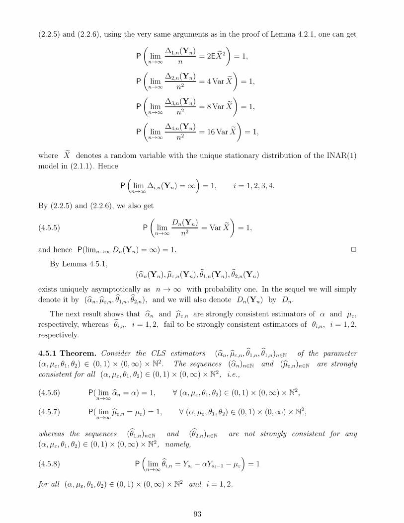
(2.2.5) and (2.2.6), using the very same arguments as in the proof of Lemma 4.2.1, one can get
P
(limn→∞
∆1,n(Yn)
n= 2EX2
)= 1,
P
(limn→∞
∆2,n(Yn)
n2= 4Var X
)= 1,
P
(limn→∞
∆3,n(Yn)
n2= 8Var X
)= 1,
P
(limn→∞
∆4,n(Yn)
n2= 16Var X
)= 1,
where X denotes a random variable with the unique stationary distribution of the INAR(1)
model in (2.1.1). Hence
P(limn→∞
∆i,n(Yn) = ∞)= 1, i = 1, 2, 3, 4.
By (2.2.5) and (2.2.6), we also get
P
(limn→∞
Dn(Yn)
n2= Var X
)= 1,(4.5.5)
and hence P(limn→∞Dn(Yn) = ∞) = 1. 2
By Lemma 4.5.1,
(αn(Yn), µε,n(Yn), θ1,n(Yn), θ2,n(Yn)
exists uniquely asymptotically as n → ∞ with probability one. In the sequel we will simply
denote it by (αn, µε,n, θ1,n, θ2,n), and we will also denote Dn(Yn) by Dn.
The next result shows that αn and µε,n are strongly consistent estimators of α and µε,
respectively, whereas θi,n, i = 1, 2, fail to be strongly consistent estimators of θi,n, i = 1, 2,
respectively.
4.5.1 Theorem. Consider the CLS estimators (αn, µε,n, θ1,n, θ1,n)n∈N of the parameter
(α, µε, θ1, θ2) ∈ (0, 1) × (0,∞) × N2. The sequences (αn)n∈N and (µε,n)n∈N are strongly
consistent for all (α, µε, θ1, θ2) ∈ (0, 1)× (0,∞)× N2, i.e.,
P( limn→∞
αn = α) = 1, ∀ (α, µε, θ1, θ2) ∈ (0, 1)× (0,∞)× N2,(4.5.6)
P( limn→∞
µε,n = µε) = 1, ∀ (α, µε, θ1, θ2) ∈ (0, 1)× (0,∞)× N2,(4.5.7)
whereas the sequences (θ1,n)n∈N and (θ2,n)n∈N are not strongly consistent for any
(α, µε, θ1, θ2) ∈ (0, 1)× (0,∞)× N2, namely,
P(limn→∞
θi,n = Ysi − αYsi−1 − µε
)= 1(4.5.8)
for all (α, µε, θ1, θ2) ∈ (0, 1)× (0,∞)× N2 and i = 1, 2.
93
Proof. To prove (4.5.6) and (4.5.7), using Proposition 4.1.2 and the proof of Theorem 4.3.1,
it is enough to check that
P
(limn→∞
1
n
n∑(s1,s2)
k=1
(Z(1)k−1 + Z
(2)k−1)(Z
(1)k + Z
(2)k ) = 0
)= 1,
P
(limn→∞
1
n2
n∑(s1,s2)
k=1
(Z(1)k−1 + Z
(2)k−1)
2 = 0
)= 1.
The above relations follows by (4.4.6).
By (4.5.4) and (4.5.6), (4.5.7), we have (4.5.8). 2
The asymptotic distribution of the CLS estimation is given in the next theorem.
4.5.2 Theorem. Under the additional assumptions EY 30 < ∞ and Eε31 < ∞, we have
[ √n(αn − α)
√n(µε,n − µε)
]L−→ N
([0
0
], Bα,ε
)as n → ∞,(4.5.9)
where Bα,ε is defined in (2.3.2). Moreover, conditionally on the values Ys1−1 and Ys2−1,
[√n(θ1,n − limk→∞ θ1,k
)√n(θ2,n − limk→∞ θ2,k
)]
L−→ N([
0
0
], Cα,εBα,εC
⊤α,ε
)as n → ∞,(4.5.10)
where
Cα,ε :=
[Ys1−1 1
Ys2−1 1
].
Proof. Using Proposition 4.1.2, the proof of Theorem 4.3.2, and (4.4.9), (4.4.10), one can
obtain (4.5.9). By (4.5.4) and (4.5.8),
[√n(θ1,n − limk→∞ θ1,k
)√n(θ2,n − limk→∞ θ2,k
)]=
√n
[Ys1 − αnYs1−1 − µε,n − (Ys1 − αYs1−1 − µε)
Ys2 − αnYs2−1 − µε,n − (Ys2 − αYs2−1 − µε)
]
=
[−Ys1−1 −1
−Ys2−1 −1
][ √n(αn − α)
√n(µε,n − µε)
]
holds asymptotically as n → ∞ with probability one. Using (4.5.9) we obtain (4.5.10). 2
5 Appendix
5.1 Lemma. If α ∈ (0, 1) and Eε1 < ∞, then the INAR(1) model in (2.1.1) has a unique
stationary distribution.
Proof. We follow the train of thoughts given in Section 6.3 in Hall and Heyde [35], but we
also complete the proof given there. For all n ∈ Z+, let Pn denote the probability generating
94
function of Xn, i.e., Pn(s) := EsXn , |s| 6 1, s ∈ C. Let A and B be the probability
generating function of the offspring (ξ1,1) and the innovation (ε1) distribution, respectively.
With the notation
A(k)(s) := (A · · · A︸ ︷︷ ︸k-times
)(s), |s| 6 1, s ∈ C, k ∈ N,
we get for all |s| 6 1, s ∈ C, and n ∈ N,
Pn(s) = E(E(sXn | FXn−1)) = E
[E(s∑Xn−1
j=1 ξn,j | FXn−1
)E(sεn | FX
n−1)]
= E(A(s)Xn−1B(s)) = Pn−1(A(s))B(s).
By iteration, we have
Pn(s) = Pn−1(A(s))B(s) = Pn−2((A A)(s))B(A(s))B(s) = · · ·
= P0(A(n)(s))B(s)
n−1∏
k=1
B(A(k)(s)), |s| 6 1, s ∈ C, n ∈ N.(5.11)
We check that limn→∞ P0(A(n)(s)) = P0(1) = 1, s ∈ C, and verify that the sequence∏n
k=1B(A(k)(s)), n ∈ N, is convergent for all s ∈ [0, 1]. By iteration, for all n ∈ N,
A(n)(s) = A(n−1)(1− α + αs) = A(n−2)(1− α + α(1− α + αs))
= A(n−2)(1− α + α(1− α) + α2s) = · · · = (1− α)n−1∑
k=0
αk + αns
= (s− 1)αn + 1,
(5.12)
and hence limn→∞A(n)(s) = 1, s ∈ C. Then limn→∞ P0(A(n)(s)) = P0(1) = 1, s ∈ C. Since
0 6 B(v) 6 1, v ∈ [0, 1], v ∈ R, we get for all s ∈ [0, 1], the sequence∏n
k=1B(A(k)(s)),
n ∈ N, is nonnegative and monotone decreasing and hence convergent.
We will use the following known theorem (see, e.g., Chung [24, Section I.6, Theorem 4 and
Section I.7, Theorem 2]. Let (ξn)n∈Z+ be a homogeneous Markov chain with state space I.
Let us suppose that there exists some subset D of I such that D is an essential, aperiodic
class and I \D is a subset of inessential states. Then either
(a) for all i ∈ I, j ∈ D we have limn→∞ p(n)i,j = 0, and therefore, there does not exist any
stationary distribution,
or
(b) for all i, j ∈ D we have limn→∞ p(n)i,j := πj > 0, and in this case the unique stationary
distribution is given by (πj)j∈I where πj := πj if j ∈ D and πj := 0 if j ∈ I \D.
Here p(n)i,j denotes the n-step transition probability from the state i to the state j.
95
Let us introduce the notation
imin := mini ∈ Z+ : P(ε1 = i) > 0
.
Using that the offspring distribution is Bernoulli, i.e., it can take values 0 and 1, and both
of them with positive probability, since α ∈ (0, 1), one can think it over that the set of states
D :=i ∈ Z+ : i > imin
is an essential class. Note also that I \D is a finite set of inessential
states. The class D is aperiodic, since
pimin,imin= P(Xn+1 = imin |Xn = imin) > P(εn+1 = imin)(1− α)imin > 0.
Note that if the additional assumption P(ε1 = 0) > 0 is satisfied, then the Markov chain is
irreducible and aperiodic.
Let us assume that there is no stationary distribution. With the notation
Pn(s) :=Pn(s)
simin=
∞∑
k=0
skP(Xn = k + imin), s ∈ [0, 1],
we get for all n ∈ N,
Pn(0) = P(Xn = imin) =∞∑
j=0
P(Xn = imin |X0 = j)P(X0 = j) =∞∑
j=0
p(n)j,imin
P(X0 = j).
Hence, by part (a) of the above recalled theorem, we get limn→∞ p(n)j,imin
= 0 for all j ∈ Z+.
Then the dominated convergence theorem yields that
limn→∞
Pn(0) = 0.
However, we show that limn→∞ Pn(0) > 0, which is a contradiction. Using that P(ε1 =
imin) > 0 and that
Pn(0) = P0(1− αn)P(ε1 = imin)
n−1∏
k=1
B(1− αk),
we have it is enough to prove that the limit of the sequence∏n
k=1B(A(k)(0)) =∏n
k=1B(1−αk),
n ∈ N, is positive. It is known that for this it is enough to verify that
∞∑
k=1
(1− B(A(k)(0))) =
∞∑
k=1
(1−B(1− αk)) is convergent,
see, e.g., Bremaud [17, Appendix, Theorem 1.9]. Just as in Section 6.3 in Hall and Heyde [35],
we show that for all s ∈ [0, 1),∑∞
k=1(1−B(A(k)(s))) is convergent. For all k ∈ N, s ∈ [0, 1),
1− B(A(k)(s)) =1− B(A(k)(s))
1−A(k)(s)(1− A(k)(s)),
and, by mean value theorem,
1−B(A(k)(s))
1− A(k)(s)=
B(A(k)(1))− B(A(k)(s))
A(k)(1)− A(k)(s)=
B′(θ(s))(A(k)(1)− A(k)(s))
A(k)(1)− A(k)(s)= B′(θ(s)),
96
with some θ(s) ∈ (s, 1). Since
B′(s) = E(ε1sε1−1) =
∞∑
k=1
ksk−1P(ε1 = k) 6
∞∑
k=1
kP(ε1 = k) = Eε1, s ∈ [0, 1],(5.13)
we have1− B(A(k)(s))
1−A(k)(s)6 Eε1 = µε, s ∈ [0, 1).
Furthermore, by (5.12), we get
1− A(k)(s) 6 1− A(k)(0) = αk, k ∈ N, s ∈ [0, 1),
and hence 1− B(A(k)(s)) 6 µεαk for all k ∈ N, s ∈ [0, 1). Then
∞∑
k=1
(1−B(A(k)(s))) 6 µε
∞∑
k=1
αk =µεα
1− α< ∞, s ∈ [0, 1).
Let us denote by X a random variable on (Ω,A, P ) with a stationary distribution for
the Markov chain (Xn)n∈Z+ . The, by the dominated convergence theorem and part (b) of the
above recalled theorem, we have for all j ∈ Z+,
limn→∞
P(Xn = j) = limn→∞
∞∑
i=0
P(Xn = j |X0 = i)P(X0 = i)
=∞∑
i=0
(limn→∞
P(Xn = j |X0 = i))P(X0 = i)
= P(X = j)
∞∑
i=0
P(X0 = i) = P(X = j),
which yields that Xn converges in distribution to X as n → ∞. By the continuity theorem
for probability generating functions (see, e.g., Feller [31, Section 11]), we also have X has the
probability generating function
P (s) := B(s)∞∏
k=1
B(A(k)(s)), s ∈ (0, 1).(5.14)
The uniqueness of the stationary distribution follows by part (b) of the above recalled theorem.
2
Proofs of formulae (2.2.3), (2.2.4) and (2.2.10). Let us introduce the probability gener-
ating functions
A(s) := Esξ = 1− α+ αs, s > 0,
where ξ is a random variable with Bernoulli distribution having parameter α ∈ (0, 1) and
B(s) := Esε =
∞∑
k=0
P(ε = k)sk, s > 0,
97
where ε is a non-negative integer-valued random variable with the same distribution as ε1.
In what follows we suppose that Eε3 < ∞. Since α ∈ (0, 1) and Eε < ∞, by Lemma 5.1,
there exists a uniquely determined stationary distribution of the INAR(1) model in (2.1.1). Let
us denote by X a random variable with this unique stationary distribution. Due to Hall and
Heyde [35, formula (6.38)] or by the proof of Lemma 5.1, the probability generating function
of X takes the form
P (s) := EsX = B(s)B(A(s))B(A(A(s))) · · · = B(s)
∞∏
k=1
B(A(k)(s)), s ∈ (0, 1),(5.15)
where for all k ∈ N,
A(k)(s) = (A · · · A︸ ︷︷ ︸k-times
)(s), s ∈ (0, 1).
Hence for all s ∈ (0, 1),
logP (s) = log EsX = logB(s) + logB(A(s)) + logB(A(A(s))) + · · ·
= logB(s) +
∞∑
k=1
logB(A(k)(s)).(5.16)
Using that Eε3 < ∞, by Abel’s theorem (see, e.g., Bremaud [17, Appendix, Theorems 1.2 and
1.3]), we get
lims↑1
(d
dslogB(s)
)= lim
s↑1
E(εsε−1)
Esε= Eε,
lims↑1
(d2
ds2logB(s)
)= lim
s↑1
E(ε(ε− 1)sε−2)Esε − (Eεsε−1)2
(Esε)2= E(ε(ε− 1))− (Eε)2,
and
lims↑1
(d3
ds3logB(s)
)= lim
s↑1
N(s)
(Esε)4,
where
N(s) :=E(ε(ε− 1)(ε− 2)sε−3)(Esε)3 + E(ε(ε− 1)sε−2)E(εsε−1)(Esε)2
−[E(ε(ε− 1)sε−2)Esε − (Eεsε−1)2
]2EsεE(εsε−1)
− 2E(εsε−1)E(ε(ε− 1)sε−2)(Esε)2, s ∈ (0, 1).
Hence
lims↑1
(d3
ds3logB(s)
)= E(ε(ε− 1)(ε− 2))− E(ε(ε− 1))Eε− 2[E(ε(ε− 1))− (Eε)2]Eε
= Eε3 − 3Eε2 + 2Eε− 3(Eε2 − Eε)Eε+ 2(Eε)3.
98
Then
Eε = lims↑1
(d
dslogB(s)
),(5.17)
Eε2 = lims↑1
(d2
ds2logB(s)
)+ Eε+ (Eε)2,(5.18)
Eε3 = lims↑1
(d3
ds3logB(s)
)+ 3Eε2 − 2Eε+ 3Eε(Eε2 − Eε)− 2(Eε)3.(5.19)
By (5.16),
logP (s) = log EsX = b(s) +∞∑
k=1
b(A(k)(s)), s ∈ (0, 1],
where b(s) := logB(s), s ∈ (0, 1]. We show that
lims↑1
(d
dslogP (s)
)= b′(1) +
∞∑
k=1
[b′(A(k)(1))
k−1∏
ℓ=0
A′(A(ℓ)(1))
].(5.20)
First we note that
d
dslogP (s) = b′(s) +
∞∑
k=1
[b′(A(k)(s))
k−1∏
ℓ=0
A′(A(ℓ)(s))
], s ∈ (0, 1),
and, by (5.12), we get for all k ∈ N, the functions b′(A(k)(s)), s ∈ [0, 1] are well-defined. We
check that the functions b′(A(k)(s)), s ∈ [0, 1], k ∈ N, are bounded with a common bound.
By (5.12), we have
A(k)(s) = (s− 1)αk + 1 ∈ [1 − αk, 1], s ∈ [0, 1], k ∈ N,
and hence A(k)(s) ∈ [1− α, 1], s ∈ [0, 1], k ∈ N. Then, using (5.13), we get
b′(A(k)(s)) =B′(A(k)(s))
B(A(k)(s))6
Eε
B(1− α)< ∞, s ∈ [0, 1], k ∈ N.
Using that A′(s) = α = Eξ, ∀ s > 0, and that
∞∑
k=1
αk =α
1− α< ∞,
the dominated convergence theorem and (5.17) yield (5.20). Hence, since A(1) = 1,
lims↑1
(d
dslogP (s)
)= Eε+ (Eε)Eξ + (Eε)(Eξ)2 + · · · =
∞∑
k=0
(Eε)(Eξ)k
=Eε
1− Eξ=
µε
1− α< ∞.
(5.21)
Just as we derived (5.17), but without supposing EX < ∞, Abel’s theorem yields that
EX = lims↑1
(d
dslogP (s)
).
99
By (5.21), we get EX = µε
1−α, which also shows that EX is finite.
Using that
b′′(s) =B′′(s)B(s)− (B′(s))2
(B(s))2, s ∈ (0, 1),
we get
b′′(A(k)(s)) 6E(ε(ε− 1))Eε
(B(1− α))2< ∞, s ∈ [0, 1], k ∈ N.
Using also that b′′(1) = E(ε(ε − 1)) − (Eε)2 and A′′(s) = 0, s > 0, by the dominated
convergence theorem, one can check that
lims↑1
(d2
ds2logP (s)
)= b′′(1) +
∞∑
k=1
b′′(A(k)(1))
(k−1∏
ℓ=0
A′(Aℓ(1))
)2
= b′′(1)
∞∑
k=0
(Eξ)2k
=E(ε(ε− 1))− (Eε)2
1− (Eξ)2=
Var ε− Eε
1− α2=
σ2ε − µε
1− α2,
which implies that EX2 is finite and
EX2 =σ2ε − µε
1− α2+
µε
1− α+
µ2ε
(1− α)2=
σ2ε + αµε
1− α2+
µ2ε
(1− α)2.
By a similar argument, using that Eε3 < ∞ and
b′′′(1) = E(ε(ε− 1)(ε− 2))− 3(Eε)(Eε(ε− 1)) + 2(Eε)3,
we get
lims↑1
(d3
ds3logP (s)
)= b′′′(1) +
∞∑
k=1
b′′′(A(k)(1))
(k−1∏
ℓ=0
A′(Aℓ(1))
)3
=E(ε(ε− 1)(ε− 2))− 3(Eε)(Eε(ε− 1)) + 2(Eε)3
1− (Eξ)3
=Eε3 − 3Eε2 + 2Eε− 3Eε(Eε2 − Eε) + 2(Eε)3
1− α3
=Eε3 − 3(σ2
ε + µ2ε) + 2µε − 3µε(σ
2ε + µ2
ε − µε) + 2µ3ε
1− α3=
Eε3 − 3σ2ε(1 + µε)− µ3
ε + 2µε
1− α3,
which implies that EX3 is finite and
EX3 =Eε3 − 3σ2
ε(1 + µε)− µ3ε + 2µε
1− α3+ 3
σ2ε + αµε
1− α2− 2
µε
1− α
+ 3µε(σ
2ε + αµε)
(1− α)(1− α2)+
µ3ε
(1− α)3.
This yields (2.2.10). One can also write (2.2.10) in the following form
EX3 =1
1− α3
[3α2(1− α)EX2 + 3α2µεEX
2 + 3αEX(σ2ε + µ2
ε) + Eε3 + 3α(1− α)µεEX
+α(1− α)(1− 2α)EX].
2
100
5.2 Lemma. Let (Xn)n∈Z+ and (Zn)n∈Z+ be two (not necessarily homogeneous) Markov
chains with state space Z+. Let us suppose that (Xn, Zn)n∈Z+ is a Markov chain, X0 and
Z0 are independent, and that for all n ∈ N and i, j, k, ℓ ∈ Z+ such that P(Xn−1 = k, Zn−1 =
ℓ) > 0,
P(Xn = i, Zn = j |Xn−1 = k, Zn−1 = ℓ) = P(Xn = i |Xn−1 = k)P(Zn = j |Zn−1 = ℓ).
Then (Xn)n∈Z+ and (Zn)n∈Z+ are independent.
Proof. For all n ∈ N and i0, i1, . . . , in, j0, j1, . . . , jn ∈ Z+, we get
P(Xn = in, . . . , X0 = i0, Zn = jn, . . . , Z0 = j0)
= P(Xn = in, Zn = jn |Xn−1 = in−1, Zn−1 = jn−1) · · ·P(X1 = i1, Z1 = j1 |X0 = i0, Z0 = j0)
× P(X0 = i0, Z0 = j0)
= P(Xn = in |Xn−1 = in−1) · · ·P(X1 = i1 |X0 = i0)P(X0 = i0)
× P(Zn = jn |Zn−1 = jn−1) · · ·P(Z1 = j1 |Z0 = j0)P(Z0 = j0)
= P(Xn = in, . . . , X0 = i0)P(Zn = jn, . . . , Z0 = j0),
which yields that Xn, . . . , X0 and Zn, . . . , Z0 are independent. One can think it over that
this implies the statement. 2
The following result can be found in several textbooks, see, e.g., Theorem 3.6 in Bhat-
tacharya and Waymire [11, Chapter 0]. For completeness we give a proof.
5.3 Lemma. Let (ξn)n∈N be a sequence of random variables such that P(limn→∞ ξn =
0) = 1 and ξpn : n ∈ N is uniformly integrable for some p ∈ N, i.e.,
limM→∞ supn∈N E(|ξn|p1|ξn|>M
)= 0. Then ξn
Lp−→ 0 as n → ∞, i.e., limn→∞ E|ξn|p = 0.
Proof. For all n ∈ N and M > 0, we get
E|ξn|p = E(|ξn|p1|ξn|p>M
)+ E
(|ξn|p1|ξn|p6M
)6 sup
n∈NE(|ξn|p1|ξn|p>M
)+ E
(|ξn|p1|ξn|p6M
).
By P(limn→∞ ξn = 0) = 1,
limn→∞
|ξn(ω)|p1|ξn(ω)|p6M = 0, ∀ ω ∈ Ω,
and E(|ξn|p1|ξn|p6M
)6 Mp < ∞ for all n ∈ N. Hence, by dominated convergence theorem,
we have
limn→∞
E(|ξn|p1|ξn|p6M
)= 0
for all M > 0. Then
lim supn→∞
E|ξn|p 6 supn∈N
E(|ξn|p1|ξn|p>M
), ∀ M > 0.
By the uniformly integrability of ξpn : n ∈ N, we have limM→∞ supn∈N E(|ξn|p1|ξn|p>M
)= 0,
which yields the assertion. 2
101
References
[1] Abraham B. and Chuang A. (1993) Expectation-maximization algorithms and the es-
timation of time series models in the presence of outliers. Journal of Time Series Analysis
14, 221–234.
[2] Ahn S., Gyemin L. and Jongwoo J. (2000) Analysis of the M/D/1-type queue based
on an integer-valued autoregressive process. Operations Research Letters 27, 235–241.
[3] Al-Osh M. A. and Alzaid A. A. (1987) First order integer-valued autoregressive
INAR(1) process. Journal of Time Series Analysis 8(3), 261–275.
[4] Al-Osh M. A. and Alzaid A. A. (1988) Integer-valued moving average (INMA) process.
Statistische Hefte 29(4), 281–300.
[5] Aly E. E. and Bouzar N. (1994) Explicit stationary distributions for some Galton-
Watson processes with immigration. Communications in Statistics. Stochastic Models
10(2), 499–517.
[6] Aly E. E. and Bouzar N. (2005) Stationary solutions for integer-valued autoregressive
processes. International Journal of Mathematics and Mathematical Sciences 1(1), 1–18.
[7] Andersson J. and Karlis D. (2010) Treating missing values in INAR(1) models: An
application to syndromic surveillance data. Journal of Time Series Analysis 31(1), 12–19.
[8] K. B. Athreya and P. E. Ney, Branching processes. Springer-Verlag, Berlin, 1972.
[9] Balke N. S. (1993) Detecting level shifts in time series. Journal of Business & Economic
Statistics 11(1), 81–92.
[10] Berkovitz L. D. (2002) Convexity and optimization in Rn. sWiley.
[11] Bhattacharya R. N. and Waymire E. C. (1990) Stochastic processes with applica-
tions. Wiley, New York.
[12] Blundell R., Griffith R. andWindmeijer F. (2002) Individual effects and dynamics
in count data models. Journal of Econometrics 108, 113–131.
[13] Brannas K. (1995) Explanatory variables in the AR(1) count data model. Umea Eco-
nomic Studies 381.
[14] Brannas K. and Hall A. (2001) Estimation in integer-valued moving average models.
Applied Stochastic Models in Business and Industry 17, 277–291.
[15] Brannas K. and Hellstrom J. (2001) Generalized integer-valued autoregression.
Econometric Reviews 20, 425–443.
[16] Brannas K. and Nordstrom J. (2006) Tourist accomodation effects of festivals.
Tourism Economics 12(2), 291–302.
102
[17] P. Bremaud, Markov chains: Gibbs fields, Monte Carlo simulation, and queues. Springer,
1999.
[18] Bu R. and McCabe B. (2008) Model selection, estimation and forecasting in INAR(p)
models: A likelihood-based Markov chain approach. International Journal of Forecasting
24(1), 151-162.
[19] Burridge P. and Taylor A. M. (2006) Additive outlier detection via extreme value
theory. Journal of Time Series Analysis 27, 685–701.
[20] Bustos O. H. and Yohai V. J. (1986) Robust estimates for ARMA models. Journal of
the American Statistical Association 81, 155–168.
[21] Cameron A. C. and Trivedi P. (1998) Regression analysis of count data. Cambridge
University Press, Oxford.
[22] Chang I., Tiao G. C. and Chen C. (1988) Estimation of time series parameters in the
presence of outliers. Technometrics 30, 193–204.
[23] Chen C. and Tiao G. C. (1990) Random level-shift time series models, ARIMA approx-
imations, and level-shift detection. Journal of Business & Economic Statistics 8, 83–97.
[24] Chung K. L. (1960) Markov chains with stationary transition probabilities. Springer.
[25] Doukhan P., Latour A. and Oraichi D. (2006) A simple integer-valued bilinear time
series model. Advances in Applied Probability 38(2), 559–578.
[26] Drost F. C., van den Akker R. and Werker B. J. M. (2009) The asymptotic
structure of nearly unstable non-negative integer-valued AR(1) models. Bernoulli 15(2),
297–324.
[27] Drost F. C., van den Akker R. and Werker B. J. M. (2009) Efficient estimation of
auto-regression parameters and innovation distributions for semiparametric integer-valued
AR(p) models. Journal of the Royal Statistical Society: Series B (Statistical Methodology)
71(2), 467–485.
[28] Drost F. C., van den Akker R. and Werker B. J. M. (2008) Local asymptotic
normality and efficient estimation for INAR(p) models. Journal of Time Series Analysis
29(5), 783–801.
[29] Drost F. C., van den Akker R. andWerker B. J. M. (2008) Note on integer-valued
bilinear time series models. Statistics & Probability Letters 78, 992–996.
[30] Du J. G. and Li Y. (1991) The integer-valued autoregressive (INAR(p)) model. Journal
of Time Series Analysis 12, 129–142.
[31] W. Feller, An introduction to probability theory and its applications, volume 1, 3rd
edition. Wiley, 1968.
[32] Fox A. J., Outliers in time series (1972) Journal of the Royal Statistical Society: Series
B (Statistical Methodology) 34, 350–363.
103

[33] Guttman I. and Tiao G. C. (1978) Effect of correlation on the estimation of a mean in
the presence of spurious observations. The Canadian Journal of Statistics 6, 229–247.
[34] Gyorfi L., Ispany M., Pap G. and Varga K. (2007) Poisson limit of an inhomoge-
neous nearly critical INAR(1) model. Acta Universitatis Szegediensis. Acta Scientiarum
Mathematicarum 73(3-4), 789–815.
[35] Hall P. and Heyde C. C. (1980) Martingale limit theory and its application. Academic
Press.
[36] Ispany M. (2008) Limit theorems for normalized nearly critical branching processes with
immigration. Publicationes Mathematicae Debrecen 72(1-2), 17–34.
[37] Ispany M., Pap G. and van Zuijlen M. (2003) Asymptotic inference for nearly unstable
INAR(1) models. Journal of Applied Probability 40(3), 750–765.
[38] Ispany M., Pap G. and van Zuijlen M. (2003) Asymptotic behaviour of estimators
of the parameters of nearly unstable INAR(1) models. Foundations of statistical inference
(Shoresh, 2000), 195–206, Contributions to Statistics, Physica, Heidelberg.
[39] Ispany M., Pap G. and van Zuijlen M. (2005) Fluctuation limit of branching processes
with immigration and estimation of the means. Advances in Applied Probability 37(2),
523–538.
[40] Jung R. C. and Tremayne A. R. (2006) Binomial thinning models for integer time
series. Statistical Modelling 6, 81-96.
[41] Kachour M. (2009) p-order rounded integer-valued autoregressive (RINAR(p)) process.
Arxiv, URL: http://arxiv.org/abs/0902.1598
[42] Kachour M. and Yao J. F. (2009) First-order rounded integer-valued autoregressive
(RINAR(1)) process. Journal of Time Series Analysis 30(4), 417–448.
[43] Klimko L. A. and Nelson P. I. (1978) On conditional least squares estimation for
stochastic processes. The Annals of Statistics 6, 629–642.
[44] Latour A. (1988) Existence and stochastic structure of a non-negative integer-valued
autoregressive processes. Journal of Time Series Analysis 4, 439–455.
[45] McCabe B. P. M. and Martin G. M. (2005) Bayesian prediction of low count time
series. International Journal of Forecasting 21, 315–330.
[46] McCulloch R. E. and Tsay R. S. (1993) Bayesian inference and prediction for mean
and variance shifts in autocovariance time series. Journal of the American Statistical As-
sociation 88, 968–978.
[47] MacDonald I. and Zucchini W. (1997) Hidden Markov and other models for discrete-
valued time series. Chapman & Hall, London.
[48] McKenzie E. (1985) Some simple models for discrete variate time series. Water Resources
Bulletin 21, 645–650.
104
[49] McKenzie E. (2003) Discrete variate time series. In: Shanbhag D. N., Rao C. R. (eds)
Handbook of Statistics. Elsevier Science, 573–606.
[50] Monteiro M., Pereira I. and Scotto M. G. (2008) Optimal alarm systems for count
processes. Communications in Statistics. Theory and Methods 37, 3054–3076.
[51] Montgomery D. C. (2005) Introduction to Statistical Quality Control, 5th edition. John
Wiley & Sons, Inc.
[52] Pena D. (2001) Outliers, influential observations, and missing data. In: Pena D., Tiao
G. C., Tsay R. S. (eds) A Course in Time Series Analysis. John Wiley & Sons, 136–170.
[53] Perron P. and Rodriguez G. (2003) Searching for additive outliers in non-stationary
time series. Journal of Time Series Analysis 24, 193-220.
[54] Quoreshi A. M. M. S. (2006) Bivariate time series modelling of financial count data.
Communications in Statistics. Theory and Methods 35, 1343–1358.
[55] Sanchez M. J. and Pena D. (2003) The identification of multiple outliers in ARIMA
models. Communications in Statistics. Theory and Methods 32, 1265–1287.
[56] Silva M. E. and Oliveira V. L. (2004) Difference equations for the higher-order mo-
ments and cumulants of the INAR(1) model. Journal of Time Series Analysis 25(3), 317–
333.
[57] Silva M. E. and Oliveira V. L. (2005) Difference equations for the higher-order mo-
ments and cumulants of the INAR(p) model. Journal of Time Series Analysis 26(1), 17–36.
[58] Silva I. and Silva M. E. (2006) Asymptotic distribution of the Yule-Walker estimator
for INAR(p) processes. Statistics & Probability Letters 76(15), 1655–1663.
[59] Silva I., Silva M. E., Pereira I. and Silva N. (2005) Replicated INAR(1) processes.
Methodology and Computing in Applied Probability 7, 517–542.
[60] Steutel F. W. and van Harn K. (1979) Discrete analogues of self–decomposability
and stability. The Annals of Probability 7, 893–99.
[61] Steutel F. W. and van Harn K. (2004) Infinite divisibility of probability distributions
on the real line. Dekker, New York.
[62] Tsay R. S. (1988) Outliers, level shifts, and variance changes in time series. Journal of
Forecasting 7, 1–20.
[63] van der Vaart A. W. (1998) Asymptotic Statistics. Cambridge University Press.
[64] Weiß C. H. (2008) Thinning operations for modelling time series of counts–a survey.
Advances in Statistical Analysis 92(3), 319-341.
[65] Weiß C. H. (2008) Serial dependence and regression of poisson INARMA models. Journal
of Statistical Planning and Inference 138, 2975-2990.
105

[66] Weiß C. H. (2008) The combined INAR(p) models for time series of counts. Statistics &
Probability Letters 78(13), 1817–1822.
[67] Zheng H. T., Basawa I. V. and Datta S. (2006) Inference for pth-order random
coefficient integer-valued autoregressive processes. Journal of Time Series Analysis 27,
411–440.
[68] Zheng H. T., Basawa I. V. andDatta S. (2007) First-order random coefficient integer-
valued autoregressive processes. Journal of Statistical Planning and Inference 173, 212–
229.
[69] Zhou J. and Basawa I. V. (2005) Least-squared estimation for bifurcation autoregressive
processes. Statistics & Probability Letters 74, 77–88.
[70] Zhu R. and Joe H. (2003) A new type of discrete self-decomposability and its applica-
tion to continuous-time Markov processes for modeling count data time series. Stochastic
Models 19(2), 235–254.
106
Related Documents