LUDWIG- MAXIMILIANS- UNIVERSITÄT MÜNCHEN DATABASE SYSTEMS GROUP INSTITUTE FOR INFORMATICS The 2010 SIAM International Conference on Data Mining Outlier Detection Techniques Hans-Peter Kriegel, Peer Kröger, Arthur Zimek Ludwig-Maximilians-Universität München Ludwig Maximilians Universität München Munich, Germany http://www.dbs.ifi.lmu.de {kriegel,kroegerp,zimek}@dbs.ifi.lmu.de Tutorial Notes: SIAM SDM 2010, Columbus, Ohio

Welcome message from author
This document is posted to help you gain knowledge. Please leave a comment to let me know what you think about it! Share it to your friends and learn new things together.
Transcript
LUDWIG-MAXIMILIANS-UNIVERSITÄTMÜNCHEN
DATABASESYSTEMSGROUP
INSTITUTE FORINFORMATICS
The 2010 SIAM International Conference on Data Mining
Outlier Detection Techniquesq
Hans-Peter Kriegel, Peer Kröger, Arthur Zimek
Ludwig-Maximilians-Universität MünchenLudwig Maximilians Universität MünchenMunich, Germany
http://www.dbs.ifi.lmu.de{kriegel,kroegerp,zimek}@dbs.ifi.lmu.de
Tutorial Notes: SIAM SDM 2010, Columbus, Ohio

DATABASESYSTEMSGROUP
General Issues
1. Please feel free to ask questions at any time during the presentation
2 Ai f th t t i l t th bi i t2. Aim of the tutorial: get the big picture– NOT in terms of a long list of methods and algorithms– BUT in terms of the basic algorithmic approaches– Sample algorithms for these basic approaches will be sketched
• The selection of the presented algorithms is somewhat arbitrary• Please don’t mind if your favorite algorithm is missingy g g• Anyway you should be able to classify any other algorithm not covered
here by means of which of the basic approaches is implemented
3 The revised version of tutorial notes will soon be available3. The revised version of tutorial notes will soon be available on our websites
2Kriegel/Kröger/Zimek: Outlier Detection Techniques (SDM 2010)

DATABASESYSTEMSGROUP
Introduction
What is an outlier?
Definition of Hawkins :Definition of Hawkins [Hawkins 1980]:“An outlier is an observation which deviates so much from the other observations as to arouse suspicions that it was generated by a different mechanism”mechanism
Statistics-based intuition– Normal data objects follow a “generating mechanism”, e.g. some
given statistical process– Abnormal objects deviate from this generating mechanism
3Kriegel/Kröger/Zimek: Outlier Detection Techniques (SDM 2010)

DATABASESYSTEMSGROUP
Introduction
• Example: Hadlum vs. Hadlum (1949) [Barnett 1978]
• The birth of a child to Mrs. Hadlum happened 349 days after Mr. Hadlum left for
ilit imilitary service.
• Average human gestation period is 280 days (40period is 280 days (40 weeks).
• Statistically 349 days is an• Statistically, 349 days is an outlier.
4Kriegel/Kröger/Zimek: Outlier Detection Techniques (SDM 2010)

DATABASESYSTEMSGROUP
Introduction
• Example: Hadlum vs. Hadlum (1949) [Barnett 1978]
blue: statistical basis (13634− blue: statistical basis (13634 observations of gestation periods)
− green: assumed underlying Gaussian processp
− Very low probability for the birth of Mrs. Hadlums child for being generated by this process
d ti f M H dl− red: assumption of Mr. Hadlum(another Gaussian process responsible for the observed birth, where the gestation period g presponsible)
− Under this assumption the gestation period has an average duration and highest-possible
5
duration and highest-possible probability
Kriegel/Kröger/Zimek: Outlier Detection Techniques (SDM 2010)

DATABASESYSTEMSGROUP
Introduction
• Sample applications of outlier detection– Fraud detection
• Purchasing behavior of a credit card owner usually changes when the• Purchasing behavior of a credit card owner usually changes when the card is stolen
• Abnormal buying patterns can characterize credit card abuse– Medicine– Medicine
• Unusual symptoms or test results may indicate potential health problems of a patient
• Whether a particular test result is abnormal may depend on otherWhether a particular test result is abnormal may depend on other characteristics of the patients (e.g. gender, age, …)
– Public health• The occurrence of a particular disease, e.g. tetanus, scattered acrossThe occurrence of a particular disease, e.g. tetanus, scattered across
various hospitals of a city indicate problems with the corresponding vaccination program in that city
• Whether an occurrence is abnormal depends on different aspects like
6
frequency, spatial correlation, etc.
Kriegel/Kröger/Zimek: Outlier Detection Techniques (SDM 2010)

DATABASESYSTEMSGROUP
Introduction
• Sample applications of outlier detection (cont.)– Sports statistics
• In many sports various parameters are recorded for players in order to• In many sports, various parameters are recorded for players in order to evaluate the players’ performances
• Outstanding (in a positive as well as a negative sense) players may be identified as having abnormal parameter valuesg p
• Sometimes, players show abnormal values only on a subset or a special combination of the recorded parameters
– Detecting measurement errorsg• Data derived from sensors (e.g. in a given scientific experiment) may
contain measurement errors• Abnormal values could provide an indication of a measurement error• Removing such errors can be important in other data mining and data
analysis tasks• “One person‘s noise could be another person‘s signal.”
7
– …
Kriegel/Kröger/Zimek: Outlier Detection Techniques (SDM 2010)

DATABASESYSTEMSGROUP
Introduction
• Discussion of the basic intuition based on Hawkins– Data is usually multivariate, i.e., multi-dimensional
=> basic model is univariate i e 1 dimensional=> basic model is univariate, i.e., 1-dimensional– There is usually more than one generating mechanism/statistical
process underlying the datab i d l l “ l” ti h i=> basic model assumes only one “normal” generating mechanism
– Anomalies may represent a different class (generating mechanism) of objects, so there may be a large class of similar objects that are the
tlioutliers=> basic model assumes that outliers are rare observations
• Consequence: a lot of models and approaches have evolved q ppin the past years in order to exceed these assumptions and it is not easy to keep track with this evolution.N d l ft i l t i l th h ll
8
• New models often involve typical, new, though usually hidden assumptions and restrictions.
Kriegel/Kröger/Zimek: Outlier Detection Techniques (SDM 2010)

DATABASESYSTEMSGROUP
Introduction
• General application scenarios– Supervised scenario
• In some applications training data with normal and abnormal data• In some applications, training data with normal and abnormal data objects are provided
• There may be multiple normal and/or abnormal classes• Often the classification problem is highly unbalancedOften, the classification problem is highly unbalanced
– Semi-supervised Scenario• In some applications, only training data for the normal class(es) (or only
the abnormal class(es)) are providedthe abnormal class(es)) are provided– Unsupervised Scenario
• In most applications there are no training data available
• In this tutorial, we focus on the unsupervised scenario
9Kriegel/Kröger/Zimek: Outlier Detection Techniques (SDM 2010)

DATABASESYSTEMSGROUP
Introduction
• Are outliers just a side product of some clustering algorithms?
Many clustering algorithms do not assign all points to clusters but– Many clustering algorithms do not assign all points to clusters but account for noise objects
– Look for outliers by applying one of those algorithms and retrieve the noise setnoise set
– Problem:• Clustering algorithms are optimized to find clusters rather than outliers• Accuracy of outlier detection depends on how good the clustering
algorithm captures the structure of clustersA t f b l d t bj t th t i il t h th ld• A set of many abnormal data objects that are similar to each other would be recognized as a cluster rather than as noise/outliers
10Kriegel/Kröger/Zimek: Outlier Detection Techniques (SDM 2010)

DATABASESYSTEMSGROUP
Introduction
• We will focus on three different classification approaches– Global versus local outlier detection
Considers the set of reference objects relative to which each point’sConsiders the set of reference objects relative to which each point s “outlierness” is judged
– Labeling versus scoring outliers– Labeling versus scoring outliersConsiders the output of an algorithm
Modeling properties– Modeling propertiesConsiders the concepts based on which “outlierness” is modeled
NOTE f d l d th d f E lid d t b tNOTE: we focus on models and methods for Euclidean data but many of those can be also used for other data types (because they only require a distance measure)
11Kriegel/Kröger/Zimek: Outlier Detection Techniques (SDM 2010)

DATABASESYSTEMSGROUP
Introduction
• Global versus local approaches– Considers the resolution of the reference set w.r.t. which the
“outlierness” of a particular data object is determinedoutlierness of a particular data object is determined– Global approaches
• The reference set contains all other data objects• Basic assumption: there is only one normal mechanism• Basic assumption: there is only one normal mechanism• Basic problem: other outliers are also in the reference set and may falsify
the resultsLocal approaches– Local approaches
• The reference contains a (small) subset of data objects• No assumption on the number of normal mechanisms• Basic problem: how to choose a proper reference set• Basic problem: how to choose a proper reference set
– NOTE: Some approaches are somewhat in between• The resolution of the reference set is varied e.g. from only a single object
(local) to the entire database (global) automatically or by a user defined
12
(local) to the entire database (global) automatically or by a user-defined input parameter
Kriegel/Kröger/Zimek: Outlier Detection Techniques (SDM 2010)

DATABASESYSTEMSGROUP
Introduction
• Labeling versus scoring– Considers the output of an outlier detection algorithm
Labeling approaches– Labeling approaches• Binary output• Data objects are labeled either as normal or outlier
S i h– Scoring approaches• Continuous output• For each object an outlier score is computed (e.g. the probability for
b i tli )being an outlier)• Data objects can be sorted according to their scores
– Notes• Many scoring approaches focus on determining the top-n outliers
(parameter n is usually given by the user)• Scoring approaches can usually also produce binary output if necessary
(e g by defining a suitable threshold on the scoring values)
13
(e.g. by defining a suitable threshold on the scoring values)
Kriegel/Kröger/Zimek: Outlier Detection Techniques (SDM 2010)

DATABASESYSTEMSGROUP
Introduction
• Approaches classified by the properties of the underlying modeling approach
Model based Approaches– Model-based Approaches• Rational
– Apply a model to represent normal data pointsOutliers are points that do not fit to that model– Outliers are points that do not fit to that model
• Sample approaches– Probabilistic tests based on statistical models– Depth-based approachesept based app oac es– Deviation-based approaches– Some subspace outlier detection approaches
14Kriegel/Kröger/Zimek: Outlier Detection Techniques (SDM 2010)

DATABASESYSTEMSGROUP
Introduction
– Proximity-based Approaches• Rational
– Examine the spatial proximity of each object in the data spacey j– If the proximity of an object considerably deviates from the proximity of other
objects it is considered an outlier • Sample approaches
Di t b d h– Distance-based approaches– Density-based approaches– Some subspace outlier detection approaches
Angle based approaches– Angle-based approaches• Rational
– Examine the spectrum of pairwise angles between a given point and all other pointsp
– Outliers are points that have a spectrum featuring high fluctuation
15Kriegel/Kröger/Zimek: Outlier Detection Techniques (SDM 2010)
DATABASESYSTEMSGROUP
Outline
1. Introduction √2. Statistical Tests
t ti ti l d l3. Depth-based Approaches4. Deviation-based Approaches5 Distance based Approaches
statistical model
5. Distance-based Approaches6. Density-based Approaches7 High-dimensional Approaches
model based on spatial proximity
adaptation of different models7. High dimensional Approaches8. Summary
to a special problem
16Kriegel/Kröger/Zimek: Outlier Detection Techniques (SDM 2010)

DATABASESYSTEMSGROUP
Statistical Tests
• General idea– Given a certain kind of statistical distribution (e.g., Gaussian)
Compute the parameters assuming all data points have been– Compute the parameters assuming all data points have been generated by such a statistical distribution (e.g., mean and standard deviation)Outliers are points that have a low probability to be generated by the– Outliers are points that have a low probability to be generated by the overall distribution (e.g., deviate more than 3 times the standard deviation from the mean)
• Basic assumption– Normal data objects follow a (known) distribution and occur in a highNormal data objects follow a (known) distribution and occur in a high
probability region of this model– Outliers deviate strongly from this distribution
17Kriegel/Kröger/Zimek: Outlier Detection Techniques (SDM 2010)

DATABASESYSTEMSGROUP
Statistical Tests
• A huge number of different tests are available differing in– Type of data distribution (e.g. Gaussian)
Number of variables i e dimensions of the data objects– Number of variables, i.e., dimensions of the data objects (univariate/multivariate)
– Number of distributions (mixture models)P t i t i ( hi t b d)– Parametric versus non-parametric (e.g. histogram-based)
• Example on the following slidesp g– Gaussian distribution– Multivariate
1 model– 1 model– Parametric
18Kriegel/Kröger/Zimek: Outlier Detection Techniques (SDM 2010)

DATABASESYSTEMSGROUP
Statistical Tests
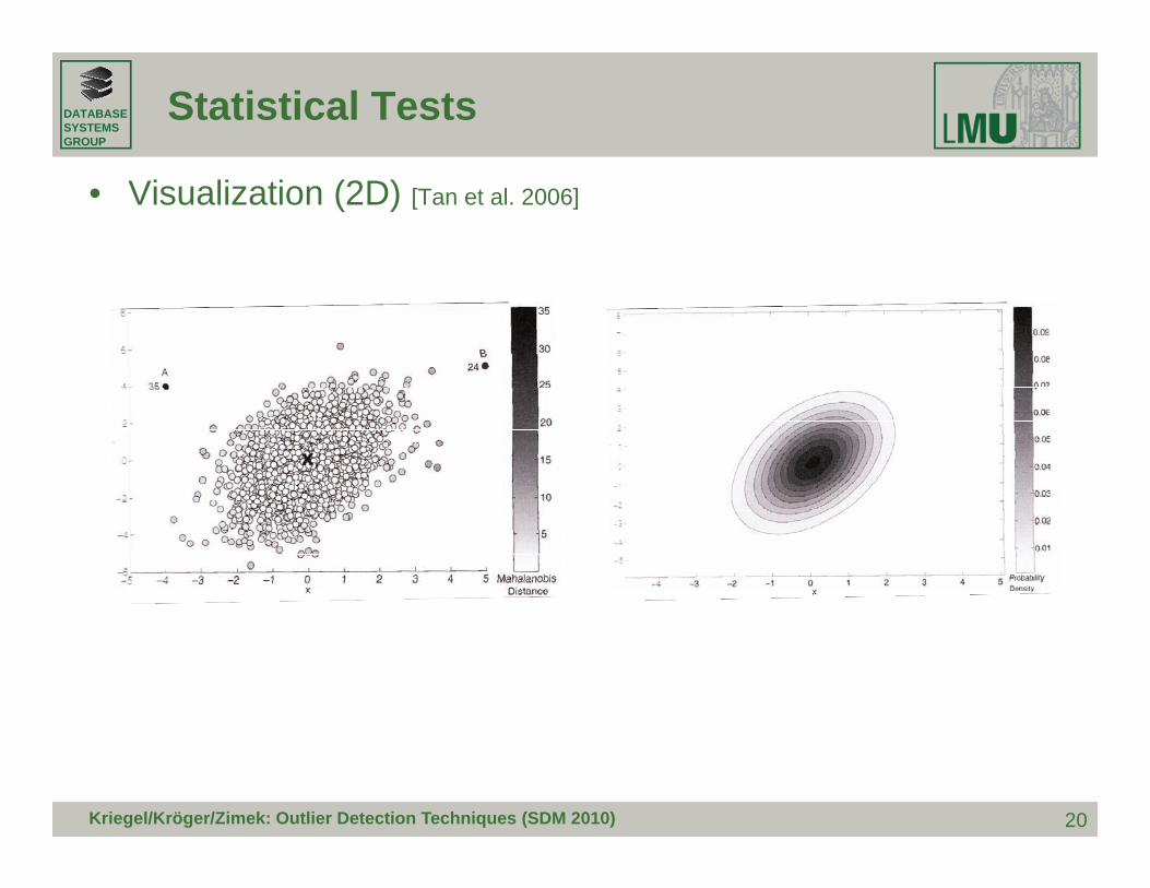
• Probability density function of a multivariate normal distribution
)()( 1 μμ − xx ΣT
( )2
)()(
||2
1)(μμ
π
−−−
Σ=
xx
dexN
Σ
– μ is the mean value of all points (usually data is normalized such that μ=0)
– Σ is the covariance matrix from the mean– is the Mahalanobis distance of
point x to μ– MDist follows a χ2-distribution with d degrees of freedom (d = data
)()(),( 1 μμμ −−= − xxxMDist ΣT
χ g (dimensionality)
– All points x, with MDist(x,μ) > χ2(0,975) [≈ 3.σ]
19Kriegel/Kröger/Zimek: Outlier Detection Techniques (SDM 2010)
DATABASESYSTEMSGROUP
Statistical Tests
• Visualization (2D) [Tan et al. 2006]
20Kriegel/Kröger/Zimek: Outlier Detection Techniques (SDM 2010)
DATABASESYSTEMSGROUP
Statistical Tests
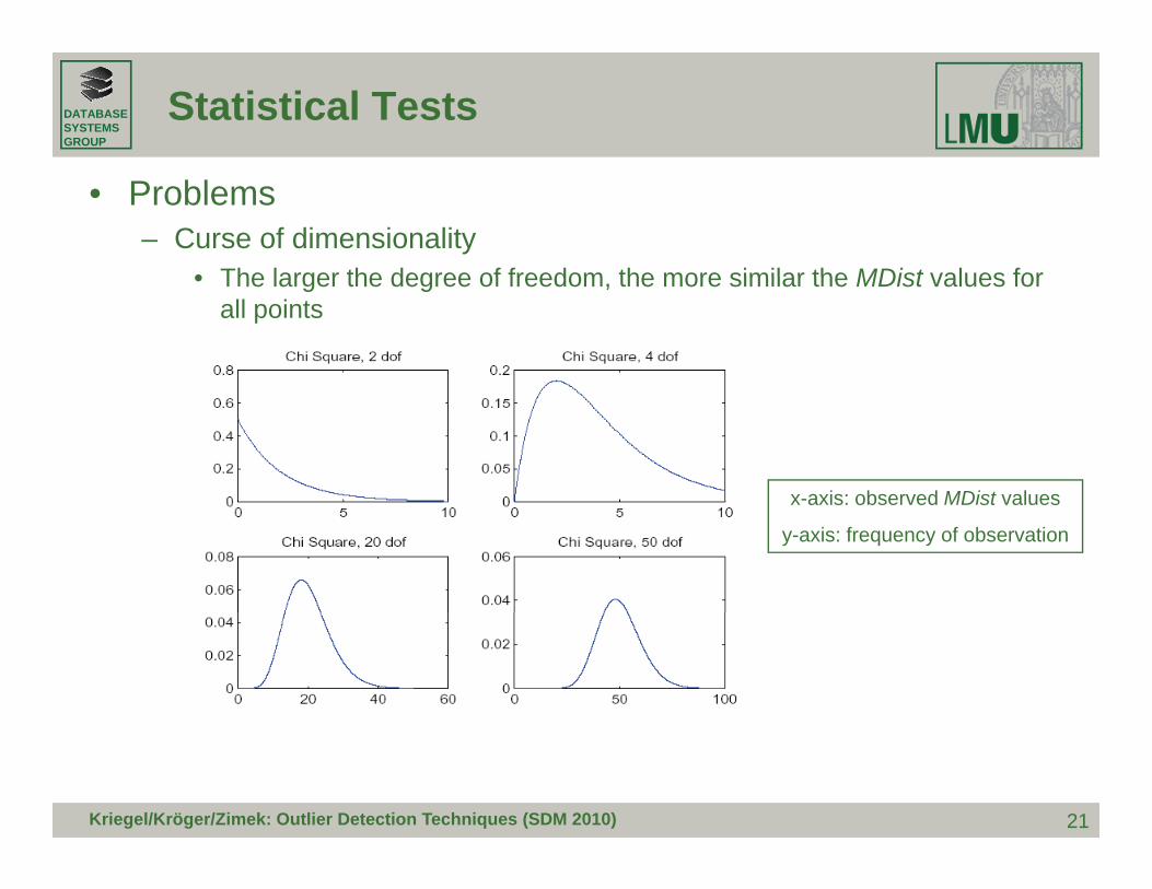
• Problems– Curse of dimensionality
• The larger the degree of freedom the more similar the MDist values for• The larger the degree of freedom, the more similar the MDist values for all points
x-axis: observed MDist valuesx axis: observed MDist values
y-axis: frequency of observation
21Kriegel/Kröger/Zimek: Outlier Detection Techniques (SDM 2010)

DATABASESYSTEMSGROUP
Statistical Tests
• Problems (cont.)– Robustness
• Mean and standard deviation are very sensitive to outliers• Mean and standard deviation are very sensitive to outliers• These values are computed for the complete data set (including potential
outliers)• The MDist is used to determine outliers although the MDist values areThe MDist is used to determine outliers although the MDist values are
influenced by these outliers=> Minimum Covariance Determinant [Rousseeuw and Leroy 1987]
minimizes the influence of outliers on the Mahalanobis distance
• Discussion– Data distribution is fixed
L fl ibili ( i d l)– Low flexibility (no mixture model)– Global method– Outputs a label but can also output a score μ
22
μDB
Kriegel/Kröger/Zimek: Outlier Detection Techniques (SDM 2010)
DATABASESYSTEMSGROUP
Outline
1. Introduction √2. Statistical Tests √3. Depth-based Approaches4. Deviation-based Approaches5 Distance based Approaches5. Distance-based Approaches6. Density-based Approaches7 High-dimensional Approaches7. High dimensional Approaches8. Summary
23Kriegel/Kröger/Zimek: Outlier Detection Techniques (SDM 2010)
DATABASESYSTEMSGROUP
Depth-based Approaches
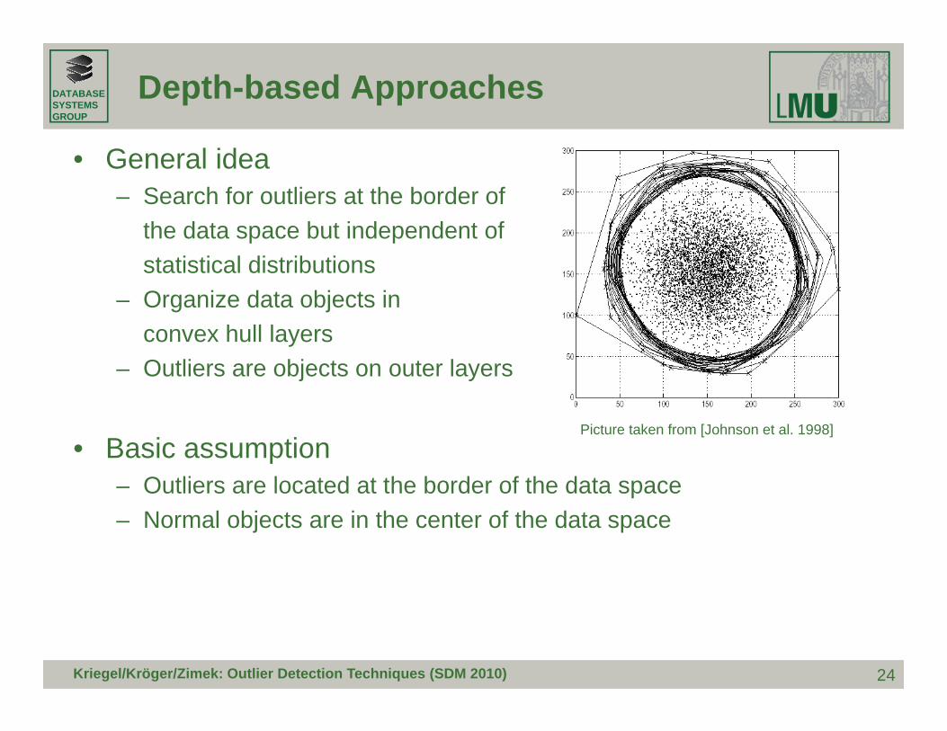
• General idea– Search for outliers at the border of
the data space but independent ofthe data space but independent ofstatistical distributions
– Organize data objects inconvex hull layers
– Outliers are objects on outer layers
• Basic assumption– Outliers are located at the border of the data space
Picture taken from [Johnson et al. 1998]
– Normal objects are in the center of the data space
24Kriegel/Kröger/Zimek: Outlier Detection Techniques (SDM 2010)

DATABASESYSTEMSGROUP
Depth-based Approaches
• Model [Tukey 1977]
– Points on the convex hull of the full data space have depth = 1Points on the convex hull of the data set after removing all points with– Points on the convex hull of the data set after removing all points with depth = 1 have depth = 2
– …P i t h i d th k t d tli– Points having a depth ≤ k are reported as outliers
Picture taken from [Preparata and Shamos 1988]
25
Picture taken from [Preparata and Shamos 1988]
Kriegel/Kröger/Zimek: Outlier Detection Techniques (SDM 2010)

DATABASESYSTEMSGROUP
Depth-based Approaches
• Sample algorithms– ISODEPTH [Ruts and Rousseeuw 1996]
FDC– FDC [Johnson et al. 1998]
• Discussion– Similar idea like classical statistical approaches (k = 1 distributions)
but independent from the chosen kind of distribution– Convex hull computation is usually only efficient in 2D / 3D spacesCo e u co putat o s usua y o y e c e t / 3 spaces– Originally outputs a label but can be extended for scoring easily (take
depth as scoring value)– Uses a global reference set for outlier detection– Uses a global reference set for outlier detection
26Kriegel/Kröger/Zimek: Outlier Detection Techniques (SDM 2010)

DATABASESYSTEMSGROUP
Outline
1. Introduction √2. Statistical Tests √
√3. Depth-based Approaches √4. Deviation-based Approaches5 Distance based Approaches5. Distance-based Approaches6. Density-based Approaches7 High-dimensional Approaches7. High dimensional Approaches8. Summary
27Kriegel/Kröger/Zimek: Outlier Detection Techniques (SDM 2010)
DATABASESYSTEMSGROUP
Deviation-based Approaches
• General idea– Given a set of data points (local group or global set)
Outliers are points that do not fit to the general characteristics of that– Outliers are points that do not fit to the general characteristics of that set, i.e., the variance of the set is minimized when removing the outliers
• Basic assumption– Outliers are the outermost points of the data set
28Kriegel/Kröger/Zimek: Outlier Detection Techniques (SDM 2010)

DATABASESYSTEMSGROUP
Deviation-based Approaches
• Model [Arning et al. 1996]
– Given a smoothing factor SF(I) that computes for each I ⊆ DB how much the variance of DB is decreased when I is removed from DBmuch the variance of DB is decreased when I is removed from DB
– With equal decrease in variance, a smaller exception set is better– The outliers are the elements of the exception set E ⊆ DB for which
the following holds:the following holds:SF(E) ≥ SF(I) for all I ⊆ DB
• Discussion:– Similar idea like classical statistical approaches (k = 1 distributions)
but independent from the chosen kind of distribution– Naïve solution is in O(2n) for n data objects( ) j– Heuristics like random sampling or best first search are applied– Applicable to any data type (depends on the definition of SF)
Originally designed as a global method
29
– Originally designed as a global method– Outputs a labeling
Kriegel/Kröger/Zimek: Outlier Detection Techniques (SDM 2010)

DATABASESYSTEMSGROUP
Outline
1. Introduction √2. Statistical Tests √
√3. Depth-based Approaches √4. Deviation-based Approaches √5 Distance based Approaches5. Distance-based Approaches6. Density-based Approaches7 High-dimensional Approaches7. High dimensional Approaches8. Summary
30Kriegel/Kröger/Zimek: Outlier Detection Techniques (SDM 2010)

DATABASESYSTEMSGROUP
Distance-based Approaches
• General Idea– Judge a point based on the distance(s) to its neighbors
Several variants proposed– Several variants proposed
• Basic AssumptionBasic Assumption– Normal data objects have a dense neighborhood– Outliers are far apart from their neighbors, i.e., have a less dense
neighborhoodneighborhood
31Kriegel/Kröger/Zimek: Outlier Detection Techniques (SDM 2010)

DATABASESYSTEMSGROUP
Distance-based Approaches
• DB(ε,π)-Outliers– Basic model [Knorr and Ng 1997]
• Given a radius ε and a percentage π• Given a radius ε and a percentage π• A point p is considered an outlier if at most π percent of all other points
have a distance to p less than ε
})(
})),(|({|{),( πεπε ≤<∈=DBCard
qpdistDBqCardpOutlierSet
range-query with radius ε
p1
ε
p2
32
p2
Kriegel/Kröger/Zimek: Outlier Detection Techniques (SDM 2010)

DATABASESYSTEMSGROUP
Distance-based Approaches
– Algorithms• Index-based [Knorr and Ng 1998]
– Compute distance range join using spatial index structureg j g– Exclude point from further consideration if its ε-neighborhood contains more
than Card(DB) . π points• Nested-loop based [Knorr and Ng 1998]
Di id b ff i t t– Divide buffer in two parts– Use second part to scan/compare all points with the points from the first part
• Grid-based [Knorr and Ng 1998]
Build grid such that any two points from the same grid cell have a distance of– Build grid such that any two points from the same grid cell have a distance of at most ε to each other
– Points need only compared with points from neighboring cells
33Kriegel/Kröger/Zimek: Outlier Detection Techniques (SDM 2010)
DATABASESYSTEMSGROUP
Distance-based Approaches
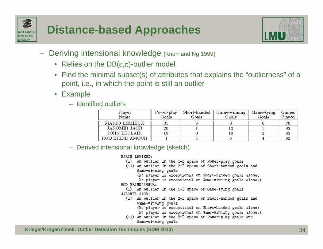
– Deriving intensional knowledge [Knorr and Ng 1999]
• Relies on the DB(ε,π)-outlier model• Find the minimal subset(s) of attributes that explains the “outlierness” of a ( ) p
point, i.e., in which the point is still an outlier• Example
– Identified outliers
– Derived intensional knowledge (sketch)
34Kriegel/Kröger/Zimek: Outlier Detection Techniques (SDM 2010)

DATABASESYSTEMSGROUP
Distance-based Approaches
• Outlier scoring based on kNN distances– General models
• Take the kNN distance of a point as its outlier score [Ramaswamy et al 2000]• Take the kNN distance of a point as its outlier score [Ramaswamy et al 2000]
• Aggregate the distances of a point to all its 1NN, 2NN, …, kNN as an outlier score [Angiulli and Pizzuti 2002]
– Algorithms– Algorithms• General approaches
– Nested-Loop» Naïve approach:» Naïve approach:
For each object: compute kNNs with a sequential scan» Enhancement: use index structures for kNN queries
– Partition-based» Partition data into micro clusters» Aggregate information for each partition (e.g. minimum bounding
rectangles)» Allows to prune micro clusters that cannot qualify when searching for the
35
» Allows to prune micro clusters that cannot qualify when searching for the kNNs of a particular point
Kriegel/Kröger/Zimek: Outlier Detection Techniques (SDM 2010)

DATABASESYSTEMSGROUP
Distance-based Approaches
– Sample Algorithms (computing top-n outliers)• Nested-Loop [Ramaswamy et al 2000]
– Simple NL algorithm with index support for kNN queriesg– Partition-based algorithm (based on a clustering algorithm that has linear
time complexity)– Algorithm for the simple kNN-distance model
Li i ti• Linearization [Angiulli and Pizzuti 2002]
– Linearization of a multi-dimensional data set using space-fill curves– 1D representation is partitioned into micro clusters– Algorithm for the average kNN-distance modelAlgorithm for the average kNN distance model
• ORCA [Bay and Schwabacher 2003]
– NL algorithm with randomization and simple pruning– Pruning: if a point has a score greater than the top-n outlier so far (cut-off), g p g p ( )
remove this point from further consideration=> non-outliers are pruned=> works good on randomized data (can be done in linear time)
> t ï NL l ith
36
=> worst-case: naïve NL algorithm– Algorithm for both kNN-distance models and the DB(ε,π)-outlier model
Kriegel/Kröger/Zimek: Outlier Detection Techniques (SDM 2010)

DATABASESYSTEMSGROUP
Distance-based Approaches
– Sample Algorithms (cont.)• RBRP [Ghoting et al. 2006],
– Idea: try to increase the cut-off as uick as possible => increase the pruning y gpower
– Compute approximate kNNs for each point to get a better cut-off– For approximate kNN search, the data points are partitioned into micro
clusters and kNNs are only searched within each micro clusterclusters and kNNs are only searched within each micro cluster– Algorithm for both kNN-distance models
• Further approaches– Also apply partitioning-based algorithms using micro clusters [McCallum et al pp y p g g g [
2000], [Tao et al. 2006]
– Approximate solution based on reference points [Pei et al. 2006]
Discussion– Discussion• Output can be a scoring (kNN-distance models) or a labeling (kNN-
distance models and the DB(ε,π)-outlier model)• Approaches are local (resolution can be adjusted by the user via ε or k)
37
• Approaches are local (resolution can be adjusted by the user via ε or k)
Kriegel/Kröger/Zimek: Outlier Detection Techniques (SDM 2010)
DATABASESYSTEMSGROUP
Distance-based Approaches
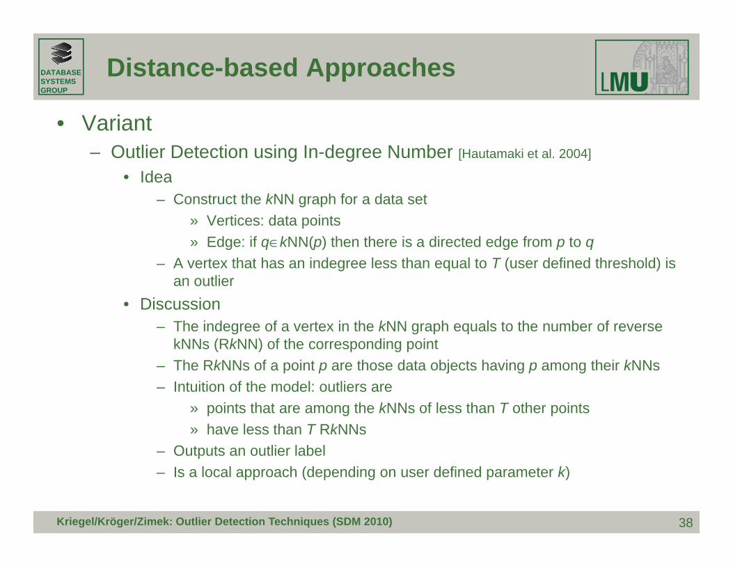
• Variant– Outlier Detection using In-degree Number [Hautamaki et al. 2004]
• Idea• Idea– Construct the kNN graph for a data set
» Vertices: data points» Edge: if q∈kNN(p) then there is a directed edge from p to qg q (p) g p q
– A vertex that has an indegree less than equal to T (user defined threshold) is an outlier
• Discussion– The indegree of a vertex in the kNN graph equals to the number of reverse
kNNs (RkNN) of the corresponding point– The RkNNs of a point p are those data objects having p among their kNNs– Intuition of the model: outliers areIntuition of the model: outliers are
» points that are among the kNNs of less than T other points» have less than T RkNNs
– Outputs an outlier label
38
– Is a local approach (depending on user defined parameter k)
Kriegel/Kröger/Zimek: Outlier Detection Techniques (SDM 2010)

DATABASESYSTEMSGROUP
Distance-based Approaches
• Resolution-based outlier factor (ROF) [Fan et al. 2006]
– Model• Depending on the resolution of applied distance thresholds points are• Depending on the resolution of applied distance thresholds, points are
outliers or within a cluster• With the maximal resolution Rmax (minimal distance threshold) all points
are outliers• With the minimal resolution Rmin (maximal distance threshold) all points
are within a cluster• Change resolution from Rmax to Rmin so that at each step at least one
point changes from being outlier to being a member of a cluster• Cluster is defined similar as in DBSCAN [Ester et al 1996] as a transitive
closure of r-neighborhoods (where r is the current resolution)• ROF value
– Discussion
∑≤≤
− −=maxmin
1
)(1)()(
RrR r
r
peclusterSizpeclusterSizpROF
39
• Outputs a score (the ROF value)• Resolution is varied automatically from local to global
Kriegel/Kröger/Zimek: Outlier Detection Techniques (SDM 2010)

DATABASESYSTEMSGROUP
Outline
1. Introduction √2. Statistical Tests √
√3. Depth-based Approaches √4. Deviation-based Approaches √5 Distance based Approaches √5. Distance-based Approaches √6. Density-based Approaches7 High-dimensional Approaches7. High dimensional Approaches8. Summary
40Kriegel/Kröger/Zimek: Outlier Detection Techniques (SDM 2010)
DATABASESYSTEMSGROUP
Density-based Approaches
• General idea– Compare the density around a point with the density around its local
neighborsneighbors– The relative density of a point compared to its neighbors is computed
as an outlier scoreApproaches also differ in how to estimate density– Approaches also differ in how to estimate density
• Basic assumption– The density around a normal data object is similar to the density
around its neighbors– The density around an outlier is considerably different to the density y y y
around its neighbors
41Kriegel/Kröger/Zimek: Outlier Detection Techniques (SDM 2010)
DATABASESYSTEMSGROUP
Density-based Approaches
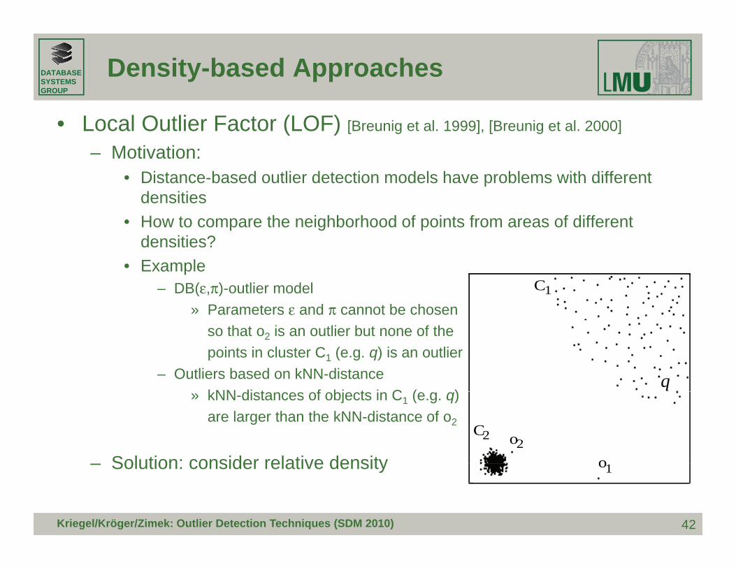
• Local Outlier Factor (LOF) [Breunig et al. 1999], [Breunig et al. 2000]
– Motivation:• Distance based outlier detection models have problems with different• Distance-based outlier detection models have problems with different
densities• How to compare the neighborhood of points from areas of different
densities?• Example
– DB(ε,π)-outlier model» Parameters ε and π cannot be chosen
C1
so that o2 is an outlier but none of thepoints in cluster C1 (e.g. q) is an outlier
– Outliers based on kNN-distancekNN di t f bj t i C ( )
q» kNN-distances of objects in C1 (e.g. q)
are larger than the kNN-distance of o2
Solution: consider relative density
C2 o2o
42
– Solution: consider relative density o1
Kriegel/Kröger/Zimek: Outlier Detection Techniques (SDM 2010)

DATABASESYSTEMSGROUP
Density-based Approaches
– Model• Reachability distance
– Introduces a smoothing factorg
• Local reachability distance (lrd) of point p
)},(),(distancemax{),( opdistokopdistreach k −=−
– Inverse of the average reach-dists of the kNNs of p
( ) ⎟⎟⎟⎞
⎜⎜⎜⎛ −
=∑
∈
)(
),(/1)( )(
pkNNCard
opdistreachplrd pkNNo
k
k
• Local outlier factor (LOF) of point p– Average ratio of lrds of neighbors of p and lrd of p
( ) ⎟⎠
⎜⎝
)( pkNNCard
Average ratio of lrds of neighbors of p and lrd of p
( ))()()(
)( )(
pkNNCardplrdolrd
pLOF pkNNo k
k
k
∑∈=
43
( ))( pkNNCard
Kriegel/Kröger/Zimek: Outlier Detection Techniques (SDM 2010)
DATABASESYSTEMSGROUP
Density-based Approaches
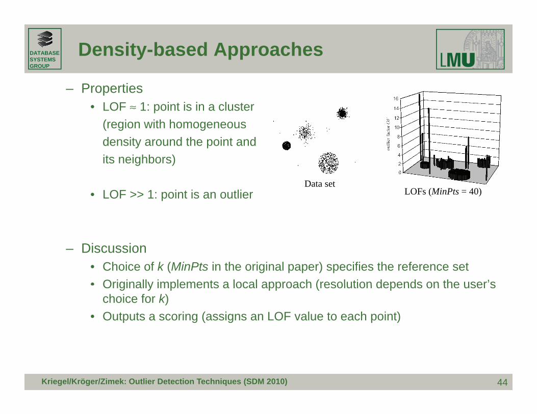
– Properties• LOF ≈ 1: point is in a cluster
(region with homogeneous( g gdensity around the point andits neighbors)
D• LOF >> 1: point is an outlier
Data setLOFs (MinPts = 40)
– Discussion• Choice of k (MinPts in the original paper) specifies the reference set• Originally implements a local approach (resolution depends on the user’sOriginally implements a local approach (resolution depends on the user s
choice for k)• Outputs a scoring (assigns an LOF value to each point)
44Kriegel/Kröger/Zimek: Outlier Detection Techniques (SDM 2010)

DATABASESYSTEMSGROUP
Density-based Approaches
• Variants of LOF– Mining top-n local outliers [Jin et al. 2001]
• Idea:• Idea:– Usually, a user is only interested in the top-n outliers– Do not compute the LOF for all data objects => save runtime
• MethodMethod– Compress data points into micro clusters using the CFs of BIRCH [Zhang et al.
1996]
– Derive upper and lower bounds of the reachability distances, lrd-values, and LOF-values for points within a micro clustersLOF-values for points within a micro clusters
– Compute upper and lower bounds of LOF values for micro clusters and sort results w.r.t. ascending lower bound
– Prune micro clusters that cannot accommodate points among the top-noutliers (n highest LOF values)
– Iteratively refine remaining micro clusters and prune points accordingly
45Kriegel/Kröger/Zimek: Outlier Detection Techniques (SDM 2010)

DATABASESYSTEMSGROUP
Density-based Approaches
• Variants of LOF (cont.)– Connectivity-based outlier factor (COF) [Tang et al. 2002]
• Motivation• Motivation– In regions of low density, it may be hard to detect outliers– Choose a low value for k is often not appropriate
• SolutionSolution– Treat “low density” and “isolation” differently
• Example
46
Data set LOF COF
Kriegel/Kröger/Zimek: Outlier Detection Techniques (SDM 2010)

DATABASESYSTEMSGROUP
Density-based Approaches
• Influenced Outlierness (INFLO) [Jin et al. 2006]
– Motivation• If clusters of different densities are not clearly separated LOF will have• If clusters of different densities are not clearly separated, LOF will have
problems
Point p will have a higher LOF than points q or r which is counter intuitive
– IdeaT k t i i hb h d l ti hi i t t
points q or r which is counter intuitive
• Take symmetric neighborhood relationship into account• Influence space (kIS(p)) of a point p includes its kNNs (kNN(p)) and its
reverse kNNs (RkNN(p))
kIS(p) = kNN(p) ∪ RkNN(p))
47
= {q1, q2, q4}
Kriegel/Kröger/Zimek: Outlier Detection Techniques (SDM 2010)

DATABASESYSTEMSGROUP
Density-based Approaches
– Model• Density is simply measured by the inverse of the kNN distance, i.e.,
den(p) = 1/k-distance(p)(p) (p)
• Influenced outlierness of a point p
)(oden∑
• INFLO takes the ratio of the average density of objects in the
)()( ))((
)(
pdenpINFLO pkISCard
k
pkISo
=∈
INFLO takes the ratio of the average density of objects in the neighborhood of a point p (i.e., in kNN(p) ∪ RkNN(p)) to p’s density
– Proposed algorithms for mining top-n outliersProposed algorithms for mining top n outliers• Index-based• Two-way approach• Micro cluster based approach
48
Micro cluster based approach
Kriegel/Kröger/Zimek: Outlier Detection Techniques (SDM 2010)

DATABASESYSTEMSGROUP
Density-based Approaches
– Properties• Similar to LOF• INFLO ≈ 1: point is in a clusterp• INFLO >> 1: point is an outlier
– Discussion• Outputs an outlier score• Originally proposed as a local approach (resolution of the reference set
kIS can be adjusted by the user setting parameter k)
49Kriegel/Kröger/Zimek: Outlier Detection Techniques (SDM 2010)

DATABASESYSTEMSGROUP
Density-based Approaches
• Local outlier correlation integral (LOCI) [Papadimitriou et al. 2003]
– Idea is similar to LOF and variantsDifferences to LOF– Differences to LOF
• Take the ε-neighborhood instead of kNNs as reference set• Test multiple resolutions (here called “granularities”) of the reference set
to get rid of any input parameterto get rid of any input parameter– Model
• ε-neighborhood of a point p: N(p,ε) = {q | dist(p,q) ≤ ε}L l d it f bj t b f bj t i N( )• Local density of an object p: number of objects in N(p,ε)
• Average density of the neighborhood)),((
)( )(εα
εqNCard
d pNq∑
∈
⋅
• Multi-granularity Deviation Factor (MDEF)
)),((),,( ),(
εαε ε
pNCardpden pNq∈=
))(())(()( εαεααε pNCardpNCardpden ⋅⋅−
50
),,()),((1
),,()),((),,(),,(
αεεα
αεεααεαε
pdenpNCard
pdenpNCardpdenpMDEF ⋅−=⋅=
Kriegel/Kröger/Zimek: Outlier Detection Techniques (SDM 2010)

DATABASESYSTEMSGROUP
Density-based Approaches
N(p,ε)
N(p1, α . ε)– Intuition
N(p,α . ε)
N(p2, α . ε)
)),((
)),((),,( ),(
ε
εααε ε
pNCard
qNCardpden pNq
∑∈
⋅=
N(p3, α . ε)
– σMDEF(p,ε,α) is the normalized standard deviation of the densities of
),,()),((1
),,()),((),,(),,(
αεεα
αεεααεαε
pdenpNCard
pdenpNCardpdenpMDEF ⋅−=⋅−=
σMDEF(p,ε,α) is the normalized standard deviation of the densities of all points from N(p,ε)
– Properties• MDEF = 0 for points within a cluster
51
MDEF 0 for points within a cluster• MDEF > 0 for outliers or MDEF > 3.σMDEF => outlier
Kriegel/Kröger/Zimek: Outlier Detection Techniques (SDM 2010)

DATABASESYSTEMSGROUP
Density-based Approaches
– Features• Parameters ε and α are automatically determined• In fact, all possible values for ε are tested, p• LOCI plot displays for a given point p the following values w.r.t. ε
– Card(N(p, α.ε))– den(p, ε, α) with a border of ± 3.σden(p, ε, α)
ε ε ε
52Kriegel/Kröger/Zimek: Outlier Detection Techniques (SDM 2010)
DATABASESYSTEMSGROUP
Density-based Approaches
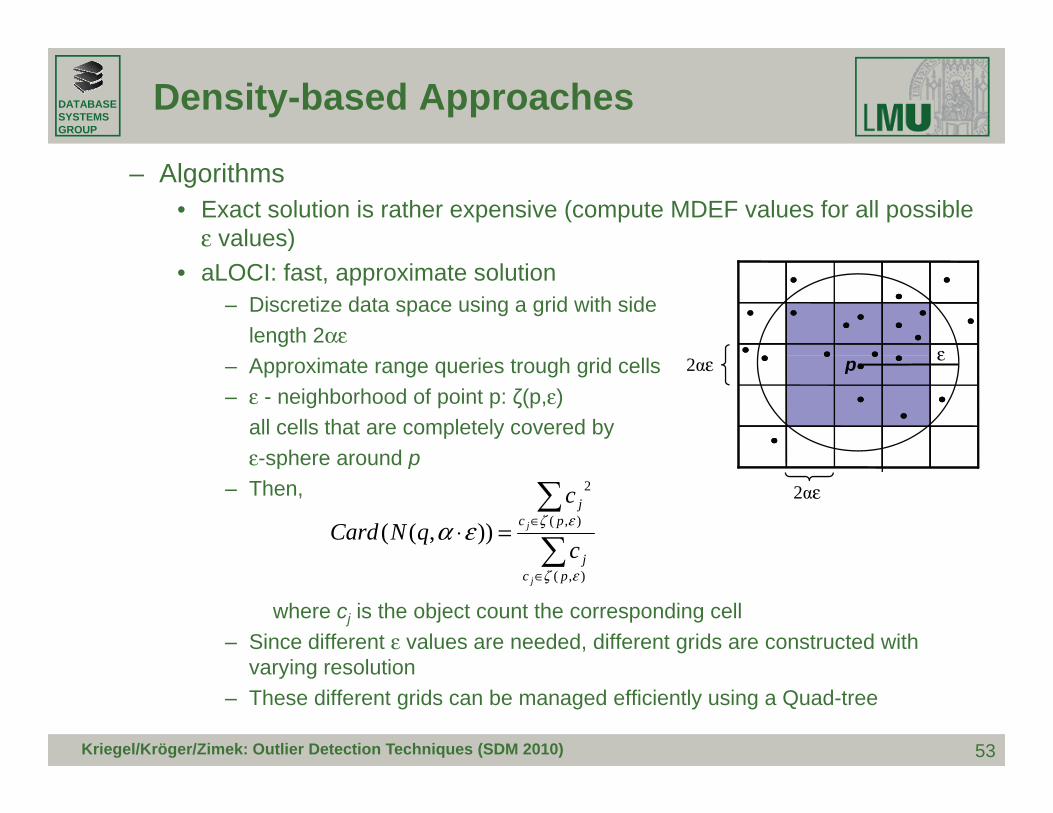
– Algorithms• Exact solution is rather expensive (compute MDEF values for all possible
ε values)• aLOCI: fast, approximate solution
– Discretize data space using a grid with sidelength 2αε
ε– Approximate range queries trough grid cells– ε - neighborhood of point p: ζ(p,ε)
all cells that are completely covered byε sphere around p
pi εp2αε
ε-sphere around p– Then, 2αε
∑
∑∈=⋅ ),(
2
)),(( εζεαj
pcj
j
c
cqNCard
where cj is the object count the corresponding cell– Since different ε values are needed, different grids are constructed with
ar ing resol tion
∑∈ ),( εζ pc
jj
53
varying resolution– These different grids can be managed efficiently using a Quad-tree
Kriegel/Kröger/Zimek: Outlier Detection Techniques (SDM 2010)

DATABASESYSTEMSGROUP
Density-based Approaches
– Discussion• Exponential runtime w.r.t. data dimensionality• Output:p
– Label: it MDEF of a point > 3.σMDEF then this point is marked as outlier– LOCI plot
» At which resolution is a point an outlier (if any)» Additional information such as diameter of clusters, distances to
clusters, etc.• All interesting resolutions, i.e., possible values for ε, (from local to global)
are testedare tested
54Kriegel/Kröger/Zimek: Outlier Detection Techniques (SDM 2010)

DATABASESYSTEMSGROUP
Outline
1. Introduction √2. Statistical Tests √
√3. Depth-based Approaches √4. Deviation-based Approaches √5 Distance based Approaches √5. Distance-based Approaches √6. Density-based Approaches √7 High-dimensional Approaches7. High dimensional Approaches8. Summary
55Kriegel/Kröger/Zimek: Outlier Detection Techniques (SDM 2010)

DATABASESYSTEMSGROUP
High-dimensional Approaches
• Challenges– Curse of dimensionality
• Relative contrast between distances decreases with increasing• Relative contrast between distances decreases with increasing dimensionality
• Data is very sparse, almost all points are outliers• Concept of neighborhood becomes meaninglessConcept of neighborhood becomes meaningless
– Solutions• Use more robust distance functions and find full dimensional outliers• Use more robust distance functions and find full-dimensional outliers• Find outliers in projections (subspaces) of the original feature space
56Kriegel/Kröger/Zimek: Outlier Detection Techniques (SDM 2010)
DATABASESYSTEMSGROUP
High-dimensional Approaches
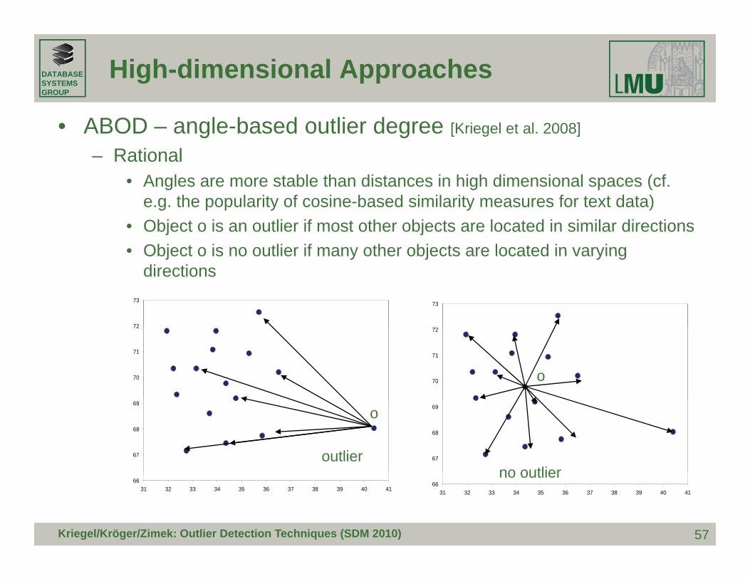
• ABOD – angle-based outlier degree [Kriegel et al. 2008]
– Rational• Angles are more stable than distances in high dimensional spaces (cf• Angles are more stable than distances in high dimensional spaces (cf.
e.g. the popularity of cosine-based similarity measures for text data)• Object o is an outlier if most other objects are located in similar directions• Object o is no outlier if many other objects are located in varyingObject o is no outlier if many other objects are located in varying
directions
72
73 73
70
71
72
70
71
72
o
67
68
69
67
68
69o
outlierno outlier
57
6631 32 33 34 35 36 37 38 39 40 41
6631 32 33 34 35 36 37 38 39 40 41
no outlier
Kriegel/Kröger/Zimek: Outlier Detection Techniques (SDM 2010)

DATABASESYSTEMSGROUP
High-dimensional Approaches
– Basic assumption• Outliers are at the border of the data distribution• Normal points are in the center of the data distributionp
– Model• Consider for a given point p the angle between
px and py for any two x y from the databasep
x
py
pyangle between px and py
px and py for any two x,y from the database• Consider the spectrum of all these angles• The broadness of this spectrum is a score for the outlierness of a point
y
0 2
0.3
1 211
-0.7
-0.2
58
-1.2
inner point outlier
Kriegel/Kröger/Zimek: Outlier Detection Techniques (SDM 2010)
DATABASESYSTEMSGROUP
High-dimensional Approaches
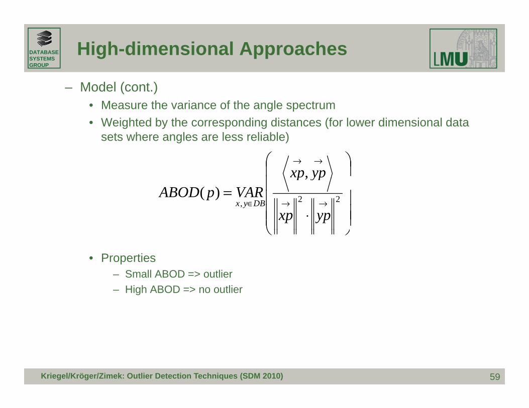
– Model (cont.)• Measure the variance of the angle spectrum• Weighted by the corresponding distances (for lower dimensional data g y p g (
sets where angles are less reliable)
⎟⎟⎞
⎜⎜⎛ →→
, ypxp
⎟⎟⎟⎟
⎠⎜⎜⎜⎜
⎝⋅
=→→∈ 22,
,)(
ypxp
yppVARpABOD
DByx
• Properties– Small ABOD => outlier
⎠⎝
– High ABOD => no outlier
59Kriegel/Kröger/Zimek: Outlier Detection Techniques (SDM 2010)

DATABASESYSTEMSGROUP
High-dimensional Approaches
– Algorithms• Naïve algorithm is in O(n3)• Approximate algorithm based on random sampling for mining top-npp g p g g p
outliers– Do not consider all pairs of other points x,y in the database to compute the
anglesC t ABOD b d l > l b d f th l ABOD– Compute ABOD based on samples => lower bound of the real ABOD
– Filter out points that have a high lower bound– Refine (compute the exact ABOD value) only for a small number of points
Discussion– Discussion• Global approach to outlier detection• Outputs an outlier score
60Kriegel/Kröger/Zimek: Outlier Detection Techniques (SDM 2010)
DATABASESYSTEMSGROUP
High-dimensional Approaches
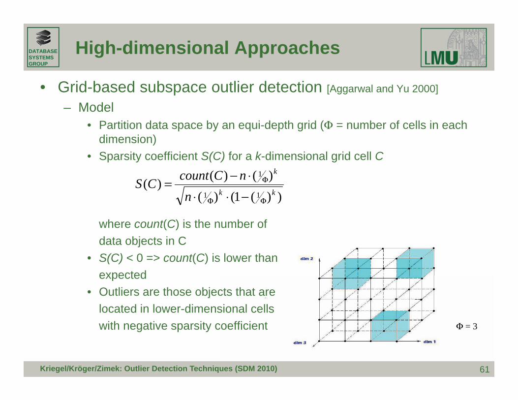
• Grid-based subspace outlier detection [Aggarwal and Yu 2000]
– Model• Partition data space by an equi depth grid (Φ = number of cells in each• Partition data space by an equi-depth grid (Φ = number of cells in each
dimension)• Sparsity coefficient S(C) for a k-dimensional grid cell C
)()( 1 knCcount
where count(C) is the number of
))(1()()()()(
11
1
kknnCcountCS
ΦΦ
Φ
−⋅⋅⋅−=
where count(C) is the number ofdata objects in C
• S(C) < 0 => count(C) is lower thanexpectedexpected
• Outliers are those objects that arelocated in lower-dimensional cellswith negative sparsity coefficient Φ = 3
61
with negative sparsity coefficient Φ = 3
Kriegel/Kröger/Zimek: Outlier Detection Techniques (SDM 2010)

DATABASESYSTEMSGROUP
High-dimensional Approaches
– Algorithm• Find the m grid cells (projections) with the lowest sparsity coefficients• Brute-force algorithm is in O(Φd)g ( )• Evolutionary algorithm (input: m and the dimensionality of the cells)
– DiscussionDiscussion• Results need not be the points from the optimal cells• Very coarse model (all objects that are in cell with less points than to be
expected)p )• Quality depends on grid resolution and grid position• Outputs a labeling• Implements a global approach (key criterion: globally expected number of p g pp ( y g y p
points within a cell)
62Kriegel/Kröger/Zimek: Outlier Detection Techniques (SDM 2010)

DATABASESYSTEMSGROUP
High-dimensional Approaches
• SOD – subspace outlier degree [Kriegel et al. 2009]
– Motivation• Outliers may be visible only in subspaces
x
x
x
A2
• Outliers may be visible only in subspacesof the original data
– ModelC t th b i hi h th
x
x
x
xxxxx
p
• Compute the subspace in which thekNNs of a point p minimize thevarianceC t th h l H (kNN( ))
xxxxxA1
A
H (kNN(p))
• Compute the hyperplane H (kNN(p))that is orthogonal to that subspace
• Take the distance of p to theh l f it
A2
pA3
x
x
x
x
dist(H (kNN(p) p)hyperplane as measure for its“outlierness”
3
xdist(H (kNN(p), p)
63
A1
Kriegel/Kröger/Zimek: Outlier Detection Techniques (SDM 2010)

DATABASESYSTEMSGROUP
High-dimensional Approaches
– Discussion• Assumes that kNNs of outliers have a lower-dimensional projection with
small variance• Resolution is local (can be adjusted by the user via the parameter k)• Output is a scoring (SOD value)
64Kriegel/Kröger/Zimek: Outlier Detection Techniques (SDM 2010)

DATABASESYSTEMSGROUP
Outline
1. Introduction √2. Statistical Tests √
√3. Depth-based Approaches √4. Deviation-based Approaches √5 Distance based Approaches √5. Distance-based Approaches √6. Density-based Approaches √7 High-dimensional Approaches √7. High dimensional Approaches √8. Summary
65Kriegel/Kröger/Zimek: Outlier Detection Techniques (SDM 2010)

DATABASESYSTEMSGROUP
Summary
• Summary– Different models are based on different assumptions to model outliers
Different models provide different types of output (labeling/scoring)– Different models provide different types of output (labeling/scoring)– Different models consider outlier at different resolutions (global/local)– Thus, different models will produce different results– A thorough and comprehensive comparison between different models
and approaches is still missing
66Kriegel/Kröger/Zimek: Outlier Detection Techniques (SDM 2010)

DATABASESYSTEMSGROUP
Summary
• Outlook– Experimental evaluation of different approaches to understand and
compare differences and common propertiescompare differences and common properties– A first step towards unification of the diverse approaches: providing
density-based outlier scores as probability values [Kriegel et al. 2009a]: judging the deviation of the outlier score from the expected valuejudging the deviation of the outlier score from the expected value
– Visualization [Achtert et al. 2010]
– New modelsP f i– Performance issues
– Complex data types– High-dimensional data– …
67Kriegel/Kröger/Zimek: Outlier Detection Techniques (SDM 2010)

DATABASESYSTEMSGROUP
Outline
1. Introduction √2. Statistical Tests √
√3. Depth-based Approaches √4. Deviation-based Approaches √5 Distance based Approaches √5. Distance-based Approaches √6. Density-based Approaches √7 High-dimensional Approaches √7. High dimensional Approaches √8. Summary √
68Kriegel/Kröger/Zimek: Outlier Detection Techniques (SDM 2010)

DATABASESYSTEMSGROUP
List of ReferencesList of References
69Kriegel/Kröger/Zimek: Outlier Detection Techniques (SDM 2010)
DATABASESYSTEMSGROUP
Literature
Achtert, E., Kriegel, H.-P., Reichert, L., Schubert, E., Wojdanowski, R., Zimek, A. 2010. Visual Evaluation of Outlier Detection Models. In Proc. International Conference on Database Systems for Advanced Applications (DASFAA), Tsukuba, Japan.
Aggarwal C C and Yu P S 2000 Outlier detection for high dimensional data In Proc ACM SIGMOD IntAggarwal, C.C. and Yu, P.S. 2000. Outlier detection for high dimensional data. In Proc. ACM SIGMOD Int. Conf. on Management of Data (SIGMOD), Dallas, TX.
Angiulli, F. and Pizzuti, C. 2002. Fast outlier detection in high dimensional spaces. In Proc. European Conf. on Principles of Knowledge Discovery and Data Mining, Helsinki, Finland.
Arning, A., Agrawal, R., and Raghavan, P. 1996. A linear method for deviation detection in large databases. In Proc. Int. Conf. on Knowledge Discovery and Data Mining (KDD), Portland, OR.
Barnett, V. 1978. The study of outliers: purpose and model. Applied Statistics, 27(3), 242–250.
Bay, S.D. and Schwabacher, M. 2003. Mining distance-based outliers in near linear time with randomization and a simple pruning rule. In Proc. Int. Conf. on Knowledge Discovery and Data Mining (KDD), Washington, DC.
Breunig, M.M., Kriegel, H.-P., Ng, R.T., and Sander, J. 1999. OPTICS-OF: identifying local outliers. In Proc. g, , g , , g, , , y gEuropean Conf. on Principles of Data Mining and Knowledge Discovery (PKDD), Prague, Czech Republic.
Breunig, M.M., Kriegel, H.-P., Ng, R.T., and Sander, J. 2000. LOF: identifying density-based local outliers. In Proc. ACM SIGMOD Int. Conf. on Management of Data (SIGMOD), Dallas, TX.
70
In Proc. ACM SIGMOD Int. Conf. on Management of Data (SIGMOD), Dallas, TX.
Kriegel/Kröger/Zimek: Outlier Detection Techniques (SDM 2010)
DATABASESYSTEMSGROUP
Literature
Ester, M., Kriegel, H.-P., Sander, J., and Xu, X. 1996. A density-based algorithm for discovering clusters in large spatial databases with noise. In Proc. Int. Conf. on Knowledge Discovery and Data Mining (KDD), Portland, OR.
Fan H Zaïane O Foss A and Wu J 2006 A nonparametric outlier detection for efficiently discoveringFan, H., Zaïane, O., Foss, A., and Wu, J. 2006. A nonparametric outlier detection for efficiently discovering top-n outliers from engineering data. In Proc. Pacific-Asia Conf. on Knowledge Discovery and Data Mining (PAKDD), Singapore.
Ghoting, A., Parthasarathy, S., and Otey, M. 2006. Fast mining of distance-based outliers in high dimensional spaces In Proc SIAM Int Conf on Data Mining (SDM) Bethesda MLdimensional spaces. In Proc. SIAM Int. Conf. on Data Mining (SDM), Bethesda, ML.
Hautamaki, V., Karkkainen, I., and Franti, P. 2004. Outlier detection using k-nearest neighbour graph. In Proc. IEEE Int. Conf. on Pattern Recognition (ICPR), Cambridge, UK.
Hawkins D 1980 Identification of Outliers Chapman and HallHawkins, D. 1980. Identification of Outliers. Chapman and Hall.
Jin, W., Tung, A., and Han, J. 2001. Mining top-n local outliers in large databases. In Proc. ACM SIGKDD Int. Conf. on Knowledge Discovery and Data Mining (SIGKDD), San Francisco, CA.
Jin, W., Tung, A., Han, J., and Wang, W. 2006. Ranking outliers using symmetric neighborhood , , g, , , , g, g g y grelationship. In Proc. Pacific-Asia Conf. on Knowledge Discovery and Data Mining (PAKDD), Singapore.
Johnson, T., Kwok, I., and Ng, R.T. 1998. Fast computation of 2-dimensional depth contours. In Proc. Int. Conf. on Knowledge Discovery and Data Mining (KDD), New York, NY.
71
Knorr, E.M. and Ng, R.T. 1997. A unified approach for mining outliers. In Proc. Conf. of the Centre for Advanced Studies on Collaborative Research (CASCON), Toronto, Canada.
Kriegel/Kröger/Zimek: Outlier Detection Techniques (SDM 2010)

DATABASESYSTEMSGROUP
Literature
Knorr, E.M. and NG, R.T. 1998. Algorithms for mining distance-based outliers in large datasets. In Proc. Int. Conf. on Very Large Data Bases (VLDB), New York, NY.
Knorr, E.M. and Ng, R.T. 1999. Finding intensional knowledge of distance-based outliers. In Proc. Int. Conf. on Very Large Data Bases (VLDB) Edinburgh Scotlandon Very Large Data Bases (VLDB), Edinburgh, Scotland.
Kriegel, H.-P., Kröger, P., Schubert, E., and Zimek, A. 2009. Outlier detection in axis-parallel subspaces of high dimensional data. In Proc. Pacific-Asia Conf. on Knowledge Discovery and Data Mining (PAKDD), Bangkok, Thailand.
Kriegel, H.-P., Kröger, P., Schubert, E., and Zimek, A. 2009a. LoOP: Local Outlier Probabilities. In Proc. ACM Conference on Information and Knowledge Management (CIKM), Hong Kong, China.
Kriegel, H.-P., Schubert, M., and Zimek, A. 2008. Angle-based outlier detection, In Proc. ACM SIGKDD Int. Conf on Knowledge Discovery and Data Mining (SIGKDD) Las Vegas NVConf. on Knowledge Discovery and Data Mining (SIGKDD), Las Vegas, NV.
McCallum, A., Nigam, K., and Ungar, L.H. 2000. Efficient clustering of high-dimensional data sets with application to reference matching. In Proc. ACM SIGKDD Int. Conf. on Knowledge Discovery and Data Mining (SIGKDD), Boston, MA.
Papadimitriou, S., Kitagawa, H., Gibbons, P., and Faloutsos, C. 2003. LOCI: Fast outlier detection using the local correlation integral. In Proc. IEEE Int. Conf. on Data Engineering (ICDE), Hong Kong, China.
Pei, Y., Zaiane, O., and Gao, Y. 2006. An efficient reference-based approach to outlier detection in large datasets. In Proc. 6th Int. Conf. on Data Mining (ICDM), Hong Kong, China.
72
datasets. In Proc. 6th Int. Conf. on Data Mining (ICDM), Hong Kong, China.
Preparata, F. and Shamos, M. 1988. Computational Geometry: an Introduction. Springer Verlag.
Kriegel/Kröger/Zimek: Outlier Detection Techniques (SDM 2010)

DATABASESYSTEMSGROUP
Literature
Ramaswamy, S. Rastogi, R. and Shim, K. 2000. Efficient algorithms for mining outliers from large data sets. In Proc. ACM SIGMOD Int. Conf. on Management of Data (SIGMOD), Dallas, TX.
Rousseeuw, P.J. and Leroy, A.M. 1987. Robust Regression and Outlier Detection. John Wiley.
Ruts, I. and Rousseeuw, P.J. 1996. Computing depth contours of bivariate point clouds. Computational Statistics and Data Analysis, 23, 153–168.
Tao Y., Xiao, X. and Zhou, S. 2006. Mining distance-based outliers from large databases in any metric space. In Proc. ACM SIGKDD Int. Conf. on Knowledge Discovery and Data Mining (SIGKDD), New space. oc. C S G t. Co . o o edge sco e y a d ata g (S G ), eYork, NY.
Tan, P.-N., Steinbach, M., and Kumar, V. 2006. Introduction to Data Mining. Addison Wesley.
Tang, J., Chen, Z., Fu, A.W.-C., and Cheung, D.W. 2002. Enhancing effectiveness of outlier detections for low density patterns. In Proc. Pacific-Asia Conf. on Knowledge Discovery and Data Mining (PAKDD), Taipei, Taiwan.
Tukey, J. 1977. Exploratory Data Analysis. Addison-Wesley.
Zhang, T., Ramakrishnan, R., Livny, M. 1996. BIRCH: an efficient data clustering method for very large databases. In Proc. ACM SIGMOD Int. Conf. on Management of Data (SIGMOD), Montreal, Canada.
73Kriegel/Kröger/Zimek: Outlier Detection Techniques (SDM 2010)
Related Documents