Outlier Detection in Multivariate Time Series by Projection Pursuit

Working Paper 04-42 Statistics and Econometrics Series 11 September 2004

Departamento de EstadísticaUniversidad Carlos III de Madrid

Calle Madrid, 12628903 Getafe (Spain)

Fax (34) 91 624-98-49

OUTLIER DETECTION IN MULTIVARIATE TIME SERIES VIA PROJECTION

PURSUIT

Pedro Galeano*, Daniel Peña* and Ruey S. Tsay** Abstract

This article uses Projection Pursuit methods to develop a procedure for detecting outliers in

a multivariate time series. We show that testing for outliers in some projection directions

could be more powerful than testing the multivariate series directly. The optimal directions

for detecting outliers are found by numerical optimization of the kurtosis coefficient of the

projected series. We propose an iterative procedure to detect and handle multiple outliers

based on univariate search in these optimal directions. In contrast with the existing methods,

the proposed procedure can identify outliers without pre-specifying a vector ARMA model

for the data. The good performance of the proposed method is verified in a Monte Carlo

study and in a real data analysis.

Keywords: Additive Outlier; Innovational Outlier; Level Change; Transitory Change; Projection Pursuit; Kurtosis coefficient. Galeano, Departamento de Estadística, Universidad Carlos III de Madrid, c/Madrid, 126, 28903 Getafe (Madrid), e-mail: [email protected]. Peña, Departamento de Estadística, Universidad Carlos III de Madrid, c/Madrid, 126, 28903 Getafe (Madrid), e-mail: [email protected]. Tsay, Graduate School of Business, University of Chicago, Chicago, IL 60637, USA, e-mail: [email protected]. The first two authors acknowledge financial support from BEC2000-0167, MCYT, Spain.

Outlier Detection in Multivariate Time Series

Via Projection Pursuit

Pedro Galeano∗, Daniel Pena∗ and Ruey S. Tsay∗∗

∗ Departamento de Estadıstica, Universidad Carlos III, Madrid, Spain

∗∗ Graduate School of Business, University of Chicago, Chicago, IL 60637, USA

Abstract

This article uses Projection Pursuit methods to develop a procedure for detecting outliers in a multi-

variate time series. We show that testing for outliers in some projection directions could be more powerful

than testing the multivariate series directly. The optimal directions for detecting outliers are found by

numerical optimization of the kurtosis coefficient of the projected series. We propose an iterative pro-

cedure to detect and handle multiple outliers based on univariate search in these optimal directions. In

contrast with the existing methods, the proposed procedure can identify outliers without pre-specifying a

vector ARMA model for the data. The good performance of the proposed method is verified in a Monte

Carlo study and in a real data analysis.

KEYWORDS: Additive Outlier; Innovational Outlier; Level Change; Transitory Change; Projection

Pursuit; Kurtosis coefficient.

1 Introduction

Outlier detection in time series analysis is an important problem because the presence of even a few anomalous

data can lead to model misspecification, biased parameter estimation and poor forecasts. Several detection

methods have been proposed for univariate time series, including Fox (1972), Chang and Tiao (1983), Tsay

(1986, 1988), Chang, Tiao and Chen (1988), Chen and Liu (1993), McCulloch and Tsay (1993, 1994), Le,

Martin and Raftery (1996), Luceno (1998), Justel, Pena and Tsay (2000), Bianco et al (2001) and Sanchez

and Pena (2003). Most of these methods are based on sequential detection procedures. For multivariate time

series Tsay, Pena and Pankratz (2000) propose a detection method based on individual and joint likelihood

1

ratio statistics.

Building adequate models for a vector time series is a difficult task, especially when the data are con-

taminated by outliers. In this paper, we propose a method to identify outliers without requiring initial

specification of the multivariate model and is based on univariate outlier detection applied to some useful

projections of the vector time series. The basic idea is simple: a multivariate outlier produces at least a uni-

variate outlier in almost every projected series, and by detecting the univariate outliers we can identify the

multivariate ones. We show that one can often identify better multivariate outliers by applying univariate

test statistics to optimal projections than using multivariate statistics to the original series. We also show

that in the presence of an outlier, the directions that maximize or minimize the kurtosis coefficient of the

projected series include the direction of the outlier, that is, the direction that maximizes the ratio between

the outlier size and the variance of the projected observations. We propose an iterative algorithm based on

projections to clean the observed series from outliers.

This paper is organized as follows. In section 2 we introduce some notation and briefly review the

multivariate outlier approach presented in Tsay et al. (2000). In section 3 we study properties of the

univariate outliers introduced by multivariate outliers through projection and discuss some advantages of

using projections to detect outliers. In section 4 we prove that the optimal directions to identify outliers

can be obtained by maximizing or minimizing the kurtosis coefficient of the projected series. In section 5 we

propose an outlier detection algorithm based on projections. We generalize the procedure to nonstationary

time series in section 6 and investigate the performance of the proposed procedure in a Monte Carlo study

in section 7. Finally, we apply the proposed method to a real data series in section 8.

2 Outliers in multivariate time series

Let Xt = (X1t, ..., Xkt)′ be a k-dimensional vector time series following the vector ARMA model

Φ (B) Xt = C + Θ(B) Et, t = 1, · · · , n, (1)

where B is the backshift operator such that BXt = Xt−1, Φ (B) = I − Φ1B − · · · − ΦpBp and Θ (B) =

I −Θ1B− · · · −ΘqBq, are k× k matrix polynomials of finite degrees p and q, C is a k-dimensional constant

vector, and Et = (E1t, ..., Ekt)′ is a sequence of independent and identically distributed Gaussian random

vectors with zero mean and positive-definite covariance matrix Σ. For the vector ARMA model in (1), we

2

have the autoregressive representation Π(B)Xt = CΠ + Et, where Π(B) = Θ(B)−1Φ(B) = I −∑∞i=1 ΠiB

i

and CΠ = Θ(1)−1C is a vector of constants if Xt is invertible, and the moving-average representation

Xt = CΨ + Ψ (B)Et, where Φ (1) CΨ = C and Φ (B) Ψ (B) = Θ (B) with Ψ(B) = I +∑∞

i=1 ΨiBi.

Given an observed time series Y = (Y ′1 , ..., Y ′

n)′, where Yt = (Y1t, ..., Ykt)′, Tsay et al. (2000) generalize

four types of univariate outliers to the vector case in a direct manner by using the representation

Yt = Xt + α (B)wI(h)t , (2)

where I(h)t is a dummy variable such that I

(h)h = 1 and I

(h)t = 0 if t 6= h, w = (w1, · · · , wk)′ is the size of

the outlier and Xt follows a vector ARMA model. The type of outlier is defined by the matrix polynomial

α (B): if α (B) = Ψ (B), we have a multivariate innovational outlier (MIO); if α (B) = I, we have a

multivariate additive outlier (MAO); if α (B) = (I −B)−1, we have a multivariate level shift (MLS); and if

α (B) = (I − δB)−1I, we have a multivariate temporary (or transitory) change (MTC), where 0 < δ < 1

is a constant. The effects of these outliers on the residuals are easily obtained when the parameters of the

vector ARMA model for Xt are known. Using the observed series and the known parameters of the model

for Xt, we obtain a series of residuals At defined by

At = Π(B)Yt − CΠ, t = 1, . . . , n,

where Yt = Xt and At = Et for t < h. The relationship between the true white noise innovations Et and the

computed residuals At is given by

At = Et + Γ (B) wI(h)t , (3)

where Γ (B) = Π (B) α (B). Tsay et al. (2000) showed that when the model is known, the estimation of the

size of a multivariate outlier of type i at time h is given by:

wi,h = −

n−h∑

j=0

Γ′jΣ−1Γj

−1

n−h∑

j=0

Γ′jΣ−1Ah+j

, i = I, A, L, T,

where Γ0 = −I. The covariance matrix of this estimate is Σi,h =(∑n−h

j=0 Γ′jΣ−1Γj

)−1

. From (3), we have

3

Ah+j = Eh+j − Γjw, and can write

wi,h = w −

n−h∑

j=0

Γ′jΣ−1Γj

−1

n−h∑

j=0

Γ′jΣ−1Eh+j

,

which implies that Σ−1/2i,h wi,h is distributed as N

(Σ−1/2

i,h w, I). Thus, the multivariate test statistic

Ji,h = wi,h′Σ−1

i,hwi,h, i = I,A, L, T (4)

will be a non-central χ2k (ηi) with noncentrality parameters ηi = w′Σ−1

i,hw, for i = I, A, L, T . In particular,

under the null hypothesis H0 : w = 0, the distribution of Ji,h will be chi-squared with k degrees of freedom.

A second statistic proposed by Tsay et al. (2000) is the maximum component statistic defined by

Ci,h = max16j6k

|wj,i,h|√σj,i,h

, i = I, A, L, T

where wj,i,h is the jth element of wi,h and σj,i,h is the jth element of the main diagonal of Σi,h.

In practice the time index h of the outlier and the parameters of the model are unknown. The parameter

matrices are then substituted by their estimates and the following overall test statistics are defined:

Jmax(i, hi) = max1≤h≤n

Ji,h, Cmax(i, h∗i ) = max1≤h≤n

Ci,h, i = I, A, L, T (5)

where hi and h∗i denote respectively the time index at which the maximum of the joint and maximum

component statistics occur.

3 Outlier analysis through projections

In this section we explore the usefulness of projections of a vector time series for outlier detection. First, we

study the relationship between the projected univariate models and the multivariate one. Second, we discuss

some potential advantages of searching for outliers in the projected series.

4

3.1 Projections of a vector ARMA model

Let us study the properties of a univariate series obtained by the projection of a multivariate series that

follows a vector ARMA model. It is well known that a non-zero linear combination of the components of

the vector ARMA model in (1) follows a univariate ARMA model; see, for instance, Lutkepohl (1993). Let

xt = v′Xt. If Xt is a vector ARMA(p, q) process, then xt follows an ARMA(p∗, q∗) model with p∗ 6 kp and

q∗ 6 (k − 1)p + q. In particular, if Xt is a vector MA(q) series, then xt is an MA(q∗) with q∗ 6 q, and if

Xt is a vector AR(p) process, then xt follows an ARMA(p∗, q∗) model with p∗ 6 kp and q∗ 6 (k − 1)p. In

general, the model of the univariate series is

φ (B)xt = c + θ (B) et, (6)

where φ (B) = |Φ(B)|, c = v′Φ(1)∗ C and v′Ω(B) Et = θ (B) et, where Φ (B)∗ is the adjoint matrix of Φ(B),

Ω(B) = Φ(B)∗Θ(B) and et is a scalar white noise process with variance σ2e . The values for θ (B) and σ2

e can

be obtained using the algorithm proposed in Maravall and Mathis (1994), which always gives an invertible

representation of the univariate process. The autoregressive representation of the univariate model (6) is

π(B)xt = cπ + et, where cπ = θ (1)−1c and π(B) = θ (B)−1

φ (B) = 1−∑∞i=1 πiB

i and its moving-average

representation is xt = cψ + ψ (B) et, where cψ = φ (1)−1c and ψ (B) = φ (B)−1

θ (B) = 1 +∑∞

i=1 ψiBi.

When the observed series Yt is affected by an outlier, as in (2), the projected series yt = v′Yt satisfies

yt = xt + v′α(B)wI(h)t . Specifically, if Yt has a multivariate additive outlier, the projected series is yt =

xt +βI(h)t so that it has an additive outlier of size β = v′w at t = h provided that v′w 6= 0. In the same way,

the projected series of a vector process with a multivariate level shift of size w will have a level shift with

size β = v′w at time t = h. The same result also applies to temporary changes. Thus, for the three types of

outliers mentioned above the following hypotheses are equivalent:

H0 : w = 0

HA : w 6= 0⇔

H∗0 : β = 0

H∗A : β 6= 0

∀v ∈ Sk − v ⊥ w

because H0 =∩H∗

0 : v ∈ Sk − v ⊥ w, where Sk =v ∈ Rk : v′v = 1

.

A multivariate innovative outlier produces a more complicated effect. It leads to a patch of consecutive

outliers with sizes v′w, v′Ψ1w, · · · , v′Ψn−hw, starting with time index t = h. Assuming that h is not close

to n and because Ψj → 0, the size of the outlier in the patch tends to zero. In the particular case that

5

0 5 10 15 20 25 300

0.2

0.4

0.6

0.8

1(a) Powers of the multivariate statistics for k=2,...,10 and the Projection statistic

w’w

0 5 10 15 20 25 300

0.1

0.2

0.3

0.4

Projection Power

k=10

k=2

(b) Difference of powers for k=2,...,10

Pro

ject

ion

Pow

er m

inus

mul

tivar

iate

pow

er

w’w

k=2

k=3

k=4

k=5 k=6

k=10 k=9

k=7 k=8

Figure 1: Powers of the Multivariate and the Projection statistics as a function of the outlier size: (a)Absolute Powers; (b) Difference of Powers.

v′Ψiw = ψiv′w, ∀i = 1, · · · , n− h, then yt has an innovational outlier at t = h with size β = v′w. However,

if v′Ψiw = 0, i = 1, . . . , n − h, then yt has an additive outlier at t = h with size w, and if v′Ψiw = v′w,

i = 0, ..., n − h, then yt has a level shift at t = h with size β = v′w. Therefore, the univariate series yt

obtained by the projection can be affected by an additive outlier, a patch of outliers or a level shift.

3.2 Some advantages of projection methods

The first advantage of using projections to search multivariate outliers is simplicity. By using univariate

series we do not need to specify a multivariate model for the underlying series in outlier detection. Second, if

the model parameters are known, a convenient projection direction will lead to test statistics that are more

powerful than the multivariate ones. Third, as will be seen later in a Monte Carlo study, the same conclusion

continues to hold when the parameters are estimated from the observed series.

To illustrate the second advantage, consider a k-dimensional time series Yt generated from the vector

ARMA model in (1) and affected by an MAO, MLS or MTC at t = h. Let V be the k × k matrix whose

first column is w/ ‖w‖ and other columns are k − 1 unit vectors orthogonal to w. The multivariate series

V ′Yt is affected by an outlier of size (‖w‖ , 0, · · · , 0)′ at time t = h. Notice that the outlier only affects the

6

first component. Because the multivariate test statistic Ji,h in (4) is invariant to linear transformations, its

value is the same for both Yt and V ′Yt series. Thus, all the information concerning the outlier is in the

first component of V ′Yt, which is the projection of the vector time series in the direction of the outlier. The

remaining components of V ′Yt are irrelevant for detecting the outlier. Moreover, because the test statistic Ji,h

is distributed as a non-central χ2k (ηi) with noncentrality parameter ηi = w′Σ−1

i,hw (i = I, A, L, T ), its power

is given by Pow (M) = Pr(Ji,h > χ2

k,α

), where χ2

k,α is the 100α percentile of the chi-square distribution with

k degrees of freedom. On the other hand, projecting the series Yt on the direction v, we obtain a series yt

affected by an outlier at time t = h, and the univariate test statistic ji,h = β2i,h/σ2

e , where βi,h is the estimate

of β, is distributed as a non-central χ21 (ηi) with noncentrality parameter ηi = β2/σ2

i,h, where β = v′w and

σ2i,h = V ar (βi,h). The power of this test statistic is Pow(U) = Pr

(ji,h > χ2

1,α

). Because the detection

procedure we propose is affine equivariant, for simplicity we assume that Yt is white noise and Σ = I. If

v = w/ ‖w‖, then it is easy to see that for every w, ηi = ηi = w′w for i = I and A, ηL = ηL = (n−h+1)w′w

and ηT = ηT =(1− δ2(n−h+1)

)/

(1− δ2

)w′w. The powers, Pow(U) and Pow (M), and their differences

Pow(U) − Pow (M) for the case of an MAO are shown in Figure 1 for different values of w′w. The figure

shows that the larger the number of components, the larger the advantage of the projection test over the

multivariate one. When the size of the outlier increases both tests have power close to one and, hence, the

difference goes to zero for large outliers. It will be seen in section 7 that for correlated series, the performance

of both multivariate and projection test statistics depend on the model. We will also compare the power of

both test statistics in section 7 via a simulation study. Finally, the same conclusion continues to hold when

the parameters are estimated from the data.

4 Finding the Projection directions

The objective of Projection Pursuit algorithms is to find interesting features of high dimensional data in

low dimensional spaces via projections. These projections are obtained by maximizing or minimizing an

objective function named projection index, which depends on the data and the projection vector. The term

interesting projection has often been associated with projections showing some unexpected structure such

as clusters, outliers or non-linear relationships among the variables. It is commonly assumed that the most

interesting projections are the farthest ones from normality. Some general reviews of Projection Pursuit

techniques can be found in Huber (1985), Jones and Sibson (1987) and Posse (1995).

Pena and Prieto (2001a) showed that given two vector random variables having symmetric distributions

7

with a common covariance matrix but different means, the direction that minimizes the kurtosis coefficient

of the projection is the linear discriminant function, that is, the direction that produces the maximum

separation between the projected means with respect to the variance of the projected distribution. These

authors also propose a procedure for multivariate outlier detection based on projections that maximize or

minimize the kurtosis coefficient of the projected data. Pena and Prieto (2001b) showed that these projected

directions are also useful to identify clusters in multivariate data.

In this section we generalize the application of projections to multivariate time series analysis and define

a maximum discrimination direction as the direction that maximizes the size of the univariate outlier, v′w,

with respect to the variance of the projected series. We show that for multivariate additive outlier, level

change and transitory change, the direction of the outlier is a direction of maximum discrimination and

this direction can be obtained by finding the extreme of the kurtosis coefficient of the projected series. For

a multivariate innovative outlier, we prove that the direction of the outlier is a maximum discrimination

direction for the residual series and it can be obtained by projecting the residuals.

Let Yt and At be the observed series and residuals in (2) and (3), respectively. For ease in presentation

and without loss of generality, we assume E(Xt) = 0 and ΣX = Cov(Xt) = I, and define the deterministic

variable,

R(h,n)t = α (B) wI

(h)t = wI

(h)t − α1wI

(h)t−1 − · · · − αn−hwI

(h)t−(n−h),

which contains two parameters, namely the time index h at which the outlier appears and the sample size

n. Projecting Yt on the direction v, we obtain yt = xt + r(h,n)t , where r

(h,n)t = v′R(h,n)

t . Let Rt and rt be

the coefficients of the variables R(h,n)t and r

(h,n)t at the time index t, respectively, that is,

Rt =

0 t < h

−αt−hw t ≥ h,rt =

0 t < h

−v′αt−hw t ≥ h,

where α0 = −I. Define R = 1n

∑nt=1 Rt and r = 1

n

∑nt=1 rt, and let

E

[1n

n∑t=1

Yt

]=

1n

(I − α1 − · · · − αn−h) w = R,

and

ΣY = E

[1n

n∑t=1

(Yt − 1

n

n∑t=1

Yt

) (Yt − 1

n

n∑t=1

Yt

)′]= I + ΣR,

8

where ΣR = 1n

∑nt=1(Rt − R)(Rt − R)′. Using the results in Rao (1973, pg. 60), the maximum of

(v′w)2 / (v′ΣY v) under the constraint v′ΣY v = 1 is v = ΣY w. In the cases of MAO, MLS and MTC,

ΣY = I + βiww′, where βi are given by

βA =n− 1n2

, βL =n− h + 1

n

(h− 1

n

), βT =

1n

[(1− δ2(n−h+1)

1− δ2

)− 1

n

(1− δ(n−h+1)

1− δ

)2]

and v = (1 + βiw′w)w, implying that v is proportional to w. The same result holds in the MIO case for

the maximum of (v′w)2 / (v′ΣAv) under the constraint v′ΣAv = 1, where ΣA is the expected value of the

covariance matrix of the innovations At.

Assuming that v verifies v′ΣY v = 1, the kurtosis coefficient of the series yt is given by

γy (v) = E

1

n

n∑t=1

(yt − 1

n

n∑

l=1

yl

)4 .

To obtain the direction of the outlier, we prove next that w can be found by maximizing or minimizing the

kurtosis coefficient γy (v). These directions are solutions to the optimization problems:

maxv′ΣY v=1

γy (v) and minv′ΣY v=1

γy (v) . (7)

To find the first-order conditions for (7), we need some preliminary results whose proofs are given in the

appendix.

Lemma 1 The kurtosis coefficient of yt can be written as

γy (v) = 3 (v′ΣY v)2 − 3 (v′ΣRv)2 + ωr (v) , (8)

where ωr (v) = 1n

∑nt=1 (rt − r)4.

Lemma 2 The extreme directions of the kurtosis coefficient of yt under the constraint v′ΣY v = 1 are given

by the eigenvectors of the matrix [n∑

t=1

βt (v)Bt

]v = µ (v) v,

where Bt =(Rt −R

) (Rt −R

)′, βt (v) = (v′Btv) − 3 (v′ΣRv) − µ(v)

n , and µ (v) = n (v′ΣRv)2 (γr (v)− 3),

where γr (v) is the kurtosis coefficient of r(h,n)t . Moreover, the directions that maximize or minimize the

9

kurtosis coefficient are given by the eigenvectors linked to the largest and the smallest eigenvalues µ (v),

respectively.

The following result shows the usefulness of the directions that maximize or minimize the kurtosis coef-

ficient of yt.

Theorem 3 Suppose Xt is a stationary vector ARMA(p, q) process and Yt = Xt + α (B)wI(h)t .

1. For a MAO, the kurtosis coefficient of yt is maximized when v is proportional to w and it is minimized

when v is orthogonal to w.

2. For a MTC, the kurtosis coefficient of yt is maximized or minimized when v is proportional to w and

it is minimized or maximized respectively when v is orthogonal to w.

3. For a MLS,

(a) the kurtosis coefficient of yt is minimized when v is proportional to w and it is maximized when

v is orthogonal to w if

h ∈(

1 +12

(1− 1√

3

)n, 1 +

12

(1 +

1√3

)n

),

(b) the kurtosis coefficient of yt is maximized when v is proportional to w and it is minimized when

v is orthogonal to w if

h /∈(

1 +12

(1− 1√

3

)n, 1 +

12

(1 +

1√3

)n

).

This theorem has two important implications. First, for a multivariate additive outlier, level shift or

transitory change, one of the directions obtained by maximizing or minimizing the kurtosis coefficient is the

direction of the outlier. Second, the directions are obtained without the information of the time index at

which the outlier occurs.

Given the characteristics of innovational outliers, it is natural to think that the direction of the outlier

can be easily obtained by focusing on the residual series. This is indeed the case.

Corollary 4 If Xt is a stationary vector ARMA(p, q) process and Yt = Xt + Ψ(B) wI(h)t and At = Et +

wI(h)t , then the kurtosis coefficient of at = v′At is maximized when v is proportional to w and it is minimized

when v is orthogonal to w.

10

On the other hand, it can be shown that the directions that produce the extreme values of the kurtosis

coefficient in the presence of multiple outliers are linear combinations of the outlier sizes. Consequently,

it would be of limited value in practice if one only considers the projections that maximize or minimize

the kurtosis coefficient because of the potential problem of masking effects. To overcome such a difficulty,

we propose to analyze a full set of 2k orthogonal directions consisting of (a) the direction that maximizes

the kurtosis coefficient, (b) the direction that minimizes the kurtosis coefficient, and (c) two sets of k − 1

orthogonal directions of (a) and (b). By doing so, if one of the outlier is masked in one direction, it can

be revealed in one of the orthogonal directions. Furthermore, after detecting the outliers in the set of 2k

orthogonal directions and cleaning their effects in the original series, we propose to iterate the analysis until

no more outliers are detected.

5 Algorithms for outliers detection

We propose here a sequential procedure for outlier detection based on the directions of maximum discrimi-

nation. The procedure is divided into four steps: (1) obtain the projections of maximum discrimination; (2)

search for outliers in the projected univariate time series; (3) all detected outliers in the univariate analysis

are considered in a multivariate model framework and their effects are removed; (4) the procedure is applied

again to the cleaned series until no more outliers are found. Note that in Step (2), the detection is carried

out in two stages: first, level shifts are identified; second, innovative outliers, additive outliers and transitory

changes are found. Finally, a vector model is identified for the cleaned time series and the outlier effects and

model parameters are jointly estimated. The fitted model is refined if necessary, e.g. removing insignificant

outliers if any.

5.1 Computation of the projection directions

We employ the procedure of Pena and Prieto (2001b) to construct the 2k projection directions of interest.

For an observed vector series Yt, our goal here is to solve the optimization problems in (7) and to obtain the

orthogonal directions of the optimal projections. To this end, consider the procedure below:

1. Let m = 1 and Z(m)t = Yt.

2. Define Z(m)

= 1n

∑nt=1 Z

(m)t and Σ(m)

Z = 1n

∑nt=1

(Z

(m)t − Z

(m))(

Z(m)t − Z

(m))′

, and find vm such

11

that

vm = arg maxv′mΣ

(m)Z vm=1

1n

n∑t=1

(v′mZ

(m)t − v′mZ

(m))4

. (9)

3. If m < k, define

Z(m+1)t =

(I − vmv′mΣ(m)

Z

)Z

(m)t ,

that is, Z(m+1)t is the projection of the observations in an orthogonal direction to vm. Let m = m + 1.

Otherwise, stop.

4. Repeat the same procedure to minimize the objective function in (9) to obtain another set of k direc-

tions; namely vk+1, . . . , v2k.

A key step of the prior algorithm is to solve the optimization problem in (9). To this end, we employ a

modified Newton method consisting of solving the system given by the first-order optimality conditions

∇γy (v)− 2λΣ(m)Z v = 0

v′Σ(m)Z v − 1 = 0,

by means of linear approximations to these conditions. We refer interested readers to Pena and Prieto

(2001b) for the technical details of the method. Note that the solutions obtained are local ones of the

problems, but our simulations show that the adopted method works well. Another relevant issue is that the

proposed procedure is affine equivariant, that is, the method selects equivalent directions for series modified

by an affine transformation.

5.2 Searching for univariate outliers

The most commonly used tests for outlier detection in univariate time series are the likelihood ratio (LR)

test statistics. Given a univariate time series yt affected by an outlier at the time point t = h, the filtered

series of residuals is defined by

at = et + γ(B)βI(h)t ,

where γ(B) = 1 −∑∞i=1 γiB

i such that γ(B) = 1 for an innovative outlier, = π(B) for an additive outlier,

= (1−B)−1π (B) for a level shift and = (1− δB)−1

π (B) for a transitory change. The likelihood ratio test

12

statistics for testing the hypothesis H0 : β = 0 versus H1 : β 6= 0 for each type of outlier are

λi,h =βi,h

ρi,hσe, i = I, A, L, T

where ρ2i,h =

(∑n−hj=0 γ2

j

)−1

with γ0 = −1 and βi,h = −ρ2i,h

(∑n−hj=0 γjah+j

)are the estimates of outlier sizes.

Because λ2i,h are the statistics Ji,h in the case of k = 1, the distributions of λ2

i,h when the parameters are

known are χ21 (ηi), where ηi =

(β

ρi,hσe

)2

.

In practice the location h of the outlier and the parameters of the model are unknown. One uses the

parameter estimates to define the overall test statistics

Λ(i, hi) = max1≤t≤n

|λi,t| , i = I, A, L, T.

Using these statistics, Chang and Tiao (1983) propose an iterative algorithm for detecting innovational and

additive outliers. Tsay (1988) generalizes the algorithm to detect level shifts and transitory changes. See

Chen and Liu (1993) and Sanchez and Pena (2003) for additional extensions.

In this paper, we consider a different approach. There is substantial evidence that using the same critical

values for all likelihood ratio test statistics can easily misidentify a level shift as an innovative outlier;

see Balke (1993) and Sanchez and Pena (2003). The latter authors showed that the critical values for the

likelihood ratio test statistic for detecting level shifts are different from those for testing additive or innovative

outliers. Therefore, we propose to identify the level shifts in a series before checking for other types of outlier.

To this end, it is necessary to develop a procedure that is capable of detecting level shifts in the presence

of the other types of outliers. Carnero et al. (2003) show that the LR test for level shifts did not work well

for financial time series and propose using a cusum test. Using the notation introduced in section 3.1, Bai

(1994) shows that the cusum statistic

Ch−1 =h− 1√nψ(1)σe

(1

h− 1

h−1∑t=1

yt − 1n

n∑t=1

yt

), (10)

converges weakly to a standard Brownian Bridge on [0, 1]. Note that Ch−1 is the statistic for testing a level

shift at t = h. In practice, the term ψ(1)σe is replaced by a consistent estimator and Bai (1994) recommends

the following estimate

ψ (1)σe =

[γ (0) + 2

K∑

i=1

(1− |i|

K

)γ (i)

] 12

,

13

where γ (h) = Cov (xt, xt−h) and K is a quantity such that K −→∞ and K/n → 0 as n →∞; see Priestley

(1981). The statistic max1≤t≤n |Ct| under the assumption of no level shifts in the sample is asymptotically

distributed as the supremum of the absolute value of a Brownian Bridge with cumulative distribution function

(Billingsley, 1968),

F (x) = 1 + 2∞∑

i=1

(−1)ie−2i2x2

, x > 0,

and Bai (1994) shows the consistency of this statistic for detecting the change point.

The cusum statistic (10) has several advantages over the LR statistic for detecting level shifts. First, the

asymptotic distribution is independent of the error distribution so the Gaussian assumption is not required.

Second, it is not necessary to specify the order of the ARMA model, which can be difficult under the presence

of level shifts. Third, as shown in section 7, this statistic seems to be more powerful than the LR in all the

models considered. Fourth, the statistic (10) seems to be robust to the presence of other outliers whereas

the LR test statistic is not.

5.2.1 Level shift detection

Given the 2k projected univariate series yt,j = v′jYt for j = 1, · · · , 2k, we propose an iterative procedure to

identify level shifts based on the algorithm proposed in Inclan and Tiao (1994) for detecting variance changes

and Carnero et al. (2003) for identifying level shifts in a white-noise financial time series. The algorithm

divides the series into pieces after detecting a level shift, and proceeds as follows:

1. Let t1 = 1.

2. Obtain

DL = max1≤i≤2k

max1≤t≤n

∣∣Cit

∣∣ , (11)

where Cit is given by (10) for t = 1, . . . , n and the 2k series. Obtain

(tmax, imax) = arg max1≤i≤2k

arg max1≤t≤n

∣∣Cit

∣∣ .

If DL > DL,α, then there is a possible level shift at t = tmax + 1, where DL,α is the critical value for

the significant level α. If DL < DL,α, then there is no level shift in the series.

14

3.a Define t2 = tmax of Step 2, and obtain

(tmax, imax) = arg max1≤i≤2k

arg max1≤t≤t2

∣∣Cit

∣∣ .

If DL > DL,α, then we redefine t2 = tmax and repeat Step 3.a until DL < DL,α. Define tfirst = t2

where t2 is the last value that attains the maximum of the cusum statistics and is larger than DL,α.

The point tfirst + 1 is the first time point with a possible level shift.

3.b We repeat a similar search in the interval t2 ≤ t ≤ n, where t2 is the point tmax obtained in Step 2.

Furthermore, define t1 = tmax + 1, where

(tmax, imax) = arg max1≤i≤2k

arg maxt1≤t≤n

∣∣Cit

∣∣ ,

and repeat the process until DL < DL,α. Let tlast = t1 − 1, where t1 is the last value that attains the

maximum of the cusum statistics and is larger than DL,α.

3.c If |tlast − tfirst| < H, where H is an integer defining the smallest interval between two level shifts,

there is just a level shift and the algorithm finishes. If not, keep both values as possible change points

and repeat the Steps 2 and 3 for t1 = tfirst and n = tlast until no more possible change points are

detected. Then, go to Step 4.

4. Define a vector hL =(hL

1 , . . . , hLrL

)where hL

1 = 1, hLrL

= n and hL2 , . . . , hL

rL−1 are the change points

detected in Steps 2 and 3 in increasing order. Obtain the statistic DL in each sub-intervals(hL

i , hLi+2

)

and check its significance. If a DL is not statistically significant, eliminate the corresponding possible

change point. Repeat Step 4 until the number of possible change points remains unchanged and the

time indexes found do not differ from those of the previous iteration for two time periods. Removing

the points hL1 = 1 and hL

rL= n from the final vector of time indexes, we obtain the time points of level

shifts by adding one to those remain in the final vector.

Some comments on the procedure are in order. First, one can rewrite the statistic (11) as

DL = max1≤i≤2k

max1≤t≤n

∣∣Cit

∣∣ = maxj=1,2

max1≤ij≤k

max1≤t≤n

∣∣∣Cij

t

∣∣∣ ,

where j is 1 for the k directions of the maximum and is 2 for the k directions of the minimum. Thus,

DL is the maximum of two dependent random variables. This dependence makes the distribution of DL

15

intractable. We obtain critical values for different significant levels via simulation in the next section.

Second, consider the number H in Steps 3.c and 4. From the definition, the test statistics (10) are highly

correlated for h close to each other. Thus, consecutive large values of Ch−1 might be caused by a single level

shift. To avoid over detection, we do not allow two level shifts to be too close. In the simulations and real

data example, we chose H to be the number of estimated parameters plus one, that is

H = k (p + q + 1) +k (k + 1)

2+ 1

and found it works well.

LethL

1 , . . . , hLrL

be the time indexes of rL detected level shifts. To remove the impacts of level shifts,

we fit the following model(I −Π1B − . . .−ΠpB

p)

Y ∗t = A∗t , (12)

where Y ∗t = Yt −

∑rL

i=1 wiS(hL

i )t , and the order p is chosen such that

p = arg min0≤p≤pmax

AIC(p) = arg min0≤p≤pmax

log

∣∣∣Σp

∣∣∣ + 2k2p

n

,

where Σp = 1n−2p−1

∑nt=p+1 A∗t A

∗′t and pmax is a prespecified upper bound. If some of the effects are

not significant, we remove the least significant one from the model (12) and re-estimate the effects of the

remaining rL − 1 level shifts. This process is repeated until all the level shifts are significant.

5.2.2 Algorithms for outliers detection

Using the level-shift adjusted series, we propose a procedure to detect additive outliers, transitory changes

and innovative outliers as follows:

1. Obtain the 2k directions that maximize or minimize the kurtosis coefficient of the projected series of

Y ∗t and their orthogonal directions. Denote the projected series by yt,j for j = 1, · · · , 2k. Obtain also

another 2k directions that maximize or minimize the kurtosis coefficient of the projected series from

the residual A∗t and their orthogonal directions. Denote the projected series by at,1, . . . , at,2k.

2. For each univariate series yt,i, we fit an autoregressive model with order selected by the Akaike in-

formation criterion (AIC). For t = 1, . . . , n, compute the test statistics, λiA,t and λi

T,t, i = 1, . . . , 2k,

using the parameter estimates of the autoregression. Obtain the maximum of the statistics∣∣λi

A,t

∣∣ and

16

∣∣λiT,t

∣∣ for each series, and then, the maxima across the series. On the other hand, for each univariate

residual series at,i, compute the test statistics∣∣λi

I,t

∣∣, where i = 1, . . . , 2k, and obtain the maximum of

the statistics∣∣λi

I,t

∣∣ over all time points and across series. Thus, we obtain

ΛA = max1≤i≤2k

max1≤t≤n

∣∣λiA,t

∣∣ , ΛT = max1≤i≤2k

max1≤t≤n

∣∣λiT,t

∣∣ , ΛI = max1≤i≤2k

max1≤t≤n

∣∣λiI,t

∣∣ . (13)

3. Let ΛA,α, ΛT,α and ΛI,α be the critical values for a predetermined significant level α. There are three

possibilities:

(a) If Λj < Λj,α, j = I, A, T , no outliers are found and go to Step 4.

(b) If Λj > Λj,α for only one j, where j = A, T, I, we identify an outlier of type j and remove its

effect using the multivariate parameter estimates.

(c) If Λj > Λj,α for more than one j, we identify the most significant outlier and remove its effect

using the multivariate parameter estimates.

We repeat Steps 1, 2, and 3 until no more outliers are detected.

4. LethA

1 , . . . , hArA

,hT

1 , . . . , hTrT

and

hI

1, . . . , hIrI

be the time indexes of the rA, rT and rI detected

additive outliers, transitory changes and innovative outliers, respectively. We estimate jointly the

model parameters and the detected outliers for the series Y ∗t :

(I −Π1B − . . .−ΠpB

p)

Y ∗∗t = A∗∗t ,

where

Y ∗∗t = Y ∗

t −rA∑

iA=1

wiAI(hA

iA)

t −rT∑

iT =1

wiT

1− δBI(hT

iT)

t , A∗∗t = A∗t −rI∑

iI=1

wiI I(hI

iI)

t .

If some of the effects are not significant, we remove the least significant outlier. This process is repeated

until all the outliers are significant.

The critical values for the statistics λiA,t, λi

T,t and λiI,t are obtained via simulation. In section 7, several

critical values for different models, number of components and sample sizes are given.

17

5.3 Final joint estimation of parameters, level shifts and outliers

By now, we have a number of detected level shifts and outliers, and proceed to perform a joint estimation

of the model parameters, the level shifts and the outliers using the equation

(I −Π1B − . . .−ΠpB

p)

Zt = Dt,

where

Zt = Yt −rL∑

iL=1

wiLS

(hLiL

)t −

rA∑

iA=1

wiAI(hA

iA)

t −rT∑

iT =1

wiT

1− δBI(hT

iT)

t , Dt = At −rI∑

iI=1

wiII(hI

iI)

t ,

andhL

1 , . . . , hLrL

,hA

1 , . . . , hArA

,hT

1 , . . . , hTrT

and

hI

1, . . . , hIrI

are the time indexes of the rL, rA, rT

and rI detected level shifts, additive outliers, transitory changes and innovative outliers, respectively. If

some effect (outlier or level shift) is found not significant at a given level, we remove the least significant

effect and repeat the joint estimation until all the effects are significant.

6 The nonstationary case

In this section we study the case that the time series is unit-root nonstationary. Assume Xt ∼ I (d1, . . . , dk),

where d1, . . . , dk are nonnegative integers denoting the degrees of differencing of the components. Suppose

that dj > 0 for at least one j. Let d = max (d1, . . . , dk) and consider first the case d = 1. For such a series,

in addition to the outliers introduced in Tsay et al. (2000) we also entertain the multivariate ramp shift

(MRS) defined by

Yt = Xt + wR(h)t

where R(h)t = (I −B)−1

S(h)t with S

(h)t being a step-function at the time index h, i.e. S

(h)t = 1 if t ≥ h and =

0 otherwise. This outlier implies a slope change in the multivariate series and it may occur in an I(1) series.

It is not expected to happen in a stationary series because the series has no time slope. Consequently, for

an MRS, we assume that it only applies to the components of Yt with dj = 1, that is, the size of the outlier

satisfies wj = 0 if dj = 0.

The series Xt can be transformed into a stationary one by taking the first difference. This transformation

affects the outlier model as follows. In the MIO case, (I −B)Yt = (I −B)Xt +Ψ (B)wI(h)t , where Ψ (B) =

∇Ψ(B). Therefore, an MIO produces an MIO in the differenced series. In the MAO case, (I −B)Yt =

18

(I −B)Xt + w(I(h)t − I

(h)t−1

), producing two consecutive MAOs with the same size but opposite signs. In

the MLS case, (I −B) Yt = (I −B)Xt + wI(h)t , resulting in an MAO of the same size. In the MTC case,

(I −B)Yt = (I −B)Xt + (I −B) (I − δB)−1wI

(h)t = (I −B) Xt + ζ (B)wI

(h)t , where ζ (B) = 1 + ζ1B +

ζ2B2 + . . . such that ζj = δj−1 (1− δ). Thus, an MTC produces an MTC with decreasing coefficients ζj . In

the MRS case, (I −B)Yt = (I −B)Xt + wS(h)t , which produces an MLS of the same size.

Note that the results in section 4 can be easily extended to these outliers. For instance, it can be shown

that the directions that maximize or minimize the kurtosis of the projected series under the presence of two

consecutive MAOs with the same size but opposite signs are the direction of the outlier or the direction

orthogonal to it. Therefore, in the I(1) case, we propose a procedure similar to that of the stationary case

for the first differenced series. The procedure consists of the following steps:

1. Take the first difference of Yt. Check for MLS as in Section 5.2.1. All the level shifts detected in the

differenced series are incorporated as ramp shifts in the original series and are estimated jointly with the

model parameters. If any of the ramp shifts is not significant, it is removed from the model. We repeat

this process until all the ramp shifts are significant. Finally, we obtain a series Y ∗t = Yt−

∑rR

i=1 wiR(h)t

which is free of ramp shifts.

2. Take the first difference of Y ∗t . The series (I −B) Y ∗

t can be affected by the outlier as

(I −B)Y ∗t = (I −B) Xt + η (B)wI

(h)t

where η (B) = Ψ (B)wI(h)t for an MIO, η (B) = w

(I(h)t − I

(h)t−1

)for an MAO, η (B) = wI

(h)t for an

MLS and η (B) = (I −B) (I − δB)−1wI

(h)t for an MTC. We then proceed as in section 5.2.2. All the

outliers detected in the differenced series are incorporated by the corresponding effect in the original

series and are estimated jointly with the model parameters. If any of the outliers is not significant, it

is removed from the model. We repeat the process until all the outliers are significant.

Note that the prior procedure can be applied to cointegrated series. In this case ∇Yt is overdifferenced,

implying that its moving average component contains unit roots. Nevertheless, this is not a problem for the

proposed procedure, because the directions of the outliers will be in general different from the directions of

cointegration. In other words, if v is a vector obtained by maximizing or minimizing the kurtosis coefficient,

then it is unlikely to be a cointegration vector, and v′∇Yt = ∇ (v′Yt) is stationary and invertible because

v′Yt is a nonstationary series. However, if the series are cointegrated, then the final estimation should be

19

carried out using the error correction model of Engle and Granger (1987):

∇Yt = C + D1∇Yt−1 + · · ·+ Dp−1∇Yt−p+1 −ΠYt−1 + At.

Note that if v is the cointegration vector, then v′Yt is stationary and ∇v′Yt is overdifferenced. Although

no relationship is expected between the outlier directions and the cointegration vector, we have checked

by Monte Carlo simulations that the probability of finding the cointegration relationship as a solution of

the optimization algorithm is very low. Specifically, we have generated 10000 series from a vector AR(1)

model with two components and a cointegration relationship and found the directions in (9). To compare

the directions with the cointegration vector, we have calculated the absolute value of the cosine of the angle

between these two directions. The average value of this cosine is 0.62 with variance 0.09. It is easy to

show that if the angle has a uniform distribution in the interval (0, π), the distribution of the cosine of

the angle has expectation 0.63 and variance 0.09. Next, we repeated the same experiment with the same

series but affected by outliers, level shifts or transitory changes and we obtained in every case that the

mean of the angles between the direction found and the cointegrating direction is the one that exits between

the direction of the outlier and the cointegration direction. Therefore, we conclude that there should be

no confusion between the cointegration vectors and the directions that maximize or minimize the kurtosis

coefficient of the projected series.

Consider next the case d = 2, i.e. the series are I(2). Define a multivariate quadratic shift as follows:

Yt = Xt + wQ(h)t

where Q(h)t = (I −B)−1

R(h)t . This outlier introduces a change in the quadratic trend of the multivariate

series. The series Xt can be transformed into a stationary one by taking the second differences. Hence

a multivariate quadratic shift is transformed into a multivariate level shift, a multivariate level shift is

transformed into a multivariate additive outlier, and so on. A similar procedure as that proposed for the

I (1) case applies. In fact, the discussion can be generalized to handle outliers in a general I(d) series.

7 Simulations and Computational Results

In this section, we investigate the computational aspects of the proposed procedures. First, we obtain critical

values for all the test statistics considered in the procedures. Second, we use various ways to compare the

20

Table 1: Models used in simulation study.

k = 2Models 1 2 3

Φ(

0.6 0.20.2 0.4

)—–

(0.6 0.20.2 0.4

)

Θ —–( −0.7 0−0.1 −0.3

) ( −0.7 0−0.1 −0.3

)

k = 3Models 4 5 6

Φ

0.6 0.2 00.2 0.4 00.6 0.2 0.5

—–

0.6 0.2 00.2 0.4 00.6 0.2 0.5

Θ —–

−0.7 0 0−0.1 −0.3 0−0.7 0 −0.5

−0.7 0 0−0.1 −0.3 0−0.7 0 −0.5

test statistics for level-shift detection. Finally, we conduct a simulation study to compare the power of the

multivariate and projection test statistics. To save space, we only show the results for the stationary case.

7.1 Critical values

We consider six VARMA(p, q) models in the simulation. The number of components is either k = 2 or k = 3,

and the parameter matrices used are given in Table 1. The constant term of the models is always the vector

1k. The residual covariance matrix is the identity matrix.

The two autoregressive parameter matrices have eigenvalues 0.27 and 0.72, and 0.27, 0.5 and 0.72,

respectively, while the moving-average parameter matrices have eigenvalues −0.3 and −0.7, and −0.3, −0.5

and −0.7, respectively. Using the six models, we generate critical values of the test statistics ΛA, ΛT and ΛI

of (13) and

DL = max1≤i≤2k

max1≤t≤n

∣∣Cit

∣∣ , ΛL = max1≤i≤2k

max1≤t≤n

∣∣λiL,t

∣∣ . (14)

The two statistics for detecting level shifts are included for comparison purpose.

The sample sizes used are n = 100, 200, and 500. For a given model and sample size, we generated

10,000 series and used the proposed procedures of the previous sections to compute the test statistics. If an

autoregression is needed in the procedures, we use AIC to select the order. Table 2 summarizes the empirical

critical values of the simulation. Based on the results, we recommend some critical values in Table 3 for

practical use to detect multivariate outliers.

21

Table 2: Empirical critical values of the test statistics considered. These values are based on sample sizes n= 100, 200, and 500 and 10,000 realizations. M denotes the models in Table 1.

95 % 99 %n M ΛI ΛA ΛL ΛT DL ΛI ΛA ΛL ΛT DL

100 1 3.62 3.93 3.22 3.78 1.33 4.02 4.30 3.61 4.16 1.44100 2 3.64 3.86 3.06 3.75 1.33 4.03 4.32 3.40 4.12 1.43100 3 3.64 3.65 3.27 3.76 1.33 3.96 4.08 3.71 4.14 1.44100 4 3.93 4.10 3.34 3.92 1.36 4.27 4.51 3.81 4.33 1.46100 5 3.97 4.20 3.23 3.92 1.36 4.32 4.62 3.72 4.35 1.46100 6 3.87 3.89 3.36 3.98 1.36 4.29 4.32 3.82 4.46 1.46200 1 3.81 3.98 3.30 3.89 1.40 4.13 4.39 3.72 4.23 1.53200 2 3.82 3.95 3.10 3.93 1.40 4.23 4.40 3.59 4.33 1.51200 3 3.79 3.84 3.34 3.87 1.40 4.08 4.14 3.71 4.20 1.52200 4 4.10 4.22 3.38 4.06 1.40 4.39 4.68 3.78 4.72 1.56200 5 4.11 4.33 3.20 4.06 1.42 4.49 4.81 3.70 4.60 1.57200 6 4.14 4.00 3.41 4.04 1.42 4.54 4.34 3.79 4.68 1.56500 1 4.08 4.18 3.41 4.19 1.44 4.52 4.65 3.91 4.64 1.61500 2 4.14 4.17 3.21 4.15 1.43 4.55 4.62 3.77 4.50 1.59500 3 4.06 4.00 3.43 4.17 1.43 4.49 4.40 3.86 4.52 1.59500 4 4.32 4.39 3.48 4.39 1.46 4.75 4.80 3.93 4.87 1.63500 5 4.26 4.42 3.38 4.33 1.47 4.79 4.87 3.83 4.76 1.66500 6 4.28 4.22 3.58 4.38 1.49 4.68 4.58 3.99 4.70 1.63

Table 3: Recommended critical values of the test statistics considered for sample size n = 100, 200 and 500.

95 % 99 %n k ΛI , ΛA, ΛT ΛL DL ΛI , ΛA, ΛT ΛL DL

100 2 3.7 3.2 1.3 4.1 3.6 1.43 4.0 3.3 1.3 4.4 3.8 1.4

200 2 3.9 3.3 1.4 4.2 3.7 1.53 4.1 3.4 1.4 4.6 3.8 1.5

500 2 4.1 3.4 1.4 4.5 3.8 1.63 4.3 3.5 1.4 4.7 3.9 1.6

22

7.2 Comparison of various test statistics for detecting level shifts

Next, we compare the performance of multivariate, LR projection and cusum test statistics for level-shift

detection. To this end, we use sample sizes n = 100 and 200, and three different outlier sizes, which are

wL = 3 × 1k, 4 × 1k and a random wL. The direction of the random wL was generated by (a) drawing a

uniform [0,1] random variable u for each component and (b) defining wL,i = −1, 0 or 1 if u is in the interval

(0, 1/3), (1/3, 2/3) or (2/3, 1). The resulting vector wL was then normalized to have the same norm as 3×1k.

For a given sample size and level shift, we generated 1000 series and computed the test statistic Jmax in

(5) for a level shift, the maximum projection statistic ΛL in (14) and the maximum cusum statistic in (14)

based on the proposed procedure. We compare the statistics with their respective critical values in Table 3

at the 5% significance level and tabulate the number of times a level shift is detected. The results are given

in the first part of Table 4 (see columns Jmax, ΛL and DL). For all the models considered, the cusum test

outperforms the other two, but all three tests seem to have decent power when the sample size is 200.

We also study the power of these three statistics in the presence of other outliers. Specifically, for each

model, we generated 1000 series of size n = 100. Each series is contaminated by an innovative outlier at

hI = 20 with size wI = w × 1k, an additive outlier at hA = 40 with size wA = −w × 1k, a transitory change

at hT = 80 with size wT = −w × 1k, and a level shift at hL = 60 with size wL = w × 1k, where w = 3 or

4. A random vector w generated by the same method as before is also used as the size for all outliers. We

compute and compare the three test statistics of level shift with their respective critical values in Table 3

at the 5% significance level. The power of these three statistics are given in the second part of Table 4 (see

columns Jmax, ΛL and DL). All three tests are affected by the presence of other outliers, but similar to the

case of a single level shift, the cusum test continues to outperform the other two test statistics. Furthermore,

we measured the power loss of each test by

loss (i) = 1− power with outliers in model i

power with no outliers in model i,

and obtained the mean power loss of the three test statistics for the 6 models used with w = 3. The

averaged loss for the multivariate statistic is 27.7%, that for the projection statistics is 17.1%, and that for

the cusum test is 9.4%. Therefore, the multivariate and projection test statistics for level shift seem to be

more susceptible to masking effects than the cusum test statistic.

Finally, it is important to study the type-I error of the three statistics in the presence of other outliers.

We use a generating procedure similar to that of power study to conduct the simulation. However, for each

23

Table 4: Frequency of properly detecting a level shift for the multivariate, projection and cusum test statistics,where n is the sample size, M denotes the model in Table 1, hi denotes time point at which a type i outlieroccurs, and w is the outlier.

w = 3× 1k w = 4× 1k w = random

n M hI hA hL hT Jmax ΛL DL Jmax ΛL DL Jmax ΛL DL

100 1 — — 50 — 70.0 83.0 100 96.6 98.2 100 68.9 83.9 100100 2 — — 50 — 58.3 82.6 100 89.2 96.9 100 67.6 94.0 100100 3 — — 50 — 46.5 73.3 87.6 91.5 93.2 100 66.9 81.6 95.3100 4 — — 50 — 93.6 92.7 99.6 100 98.8 100 83.6 87.6 99.7100 5 — — 50 — 68.1 98.8 100 94.7 99.7 100 76.9 91.3 100100 6 — — 50 — 86.3 86.6 88.7 98.9 99.0 99.2 78.2 77.2 96.7200 1 — — 100 — 80.7 95.4 100 98.1 99.6 100 90.3 91.0 100200 2 — — 100 — 92.2 95.6 100 97.0 99.3 100 88.3 98.0 100200 3 — — 100 — 78.1 90.6 99.5 97.1 98.4 100 80.9 84.6 100200 4 — — 100 — 98.7 98.9 100 100 100 100 90.6 94.0 100200 5 — — 100 — 85.8 99.8 100 99.0 100 100 89.3 98.7 100200 6 — — 100 — 97.5 97.8 100 99.6 99.7 100 90.3 83.6 100100 1 20 40 60 80 45.6 76.0 92.6 73.0 91.8 99.3 55.2 70.9 95.7100 2 20 40 60 80 52.0 87.6 100 74.3 96.7 100 58.9 77.6 99.7100 3 20 40 60 80 17.0 53.6 66.6 40.3 84.3 86.6 44.1 49.2 80.9100 4 20 40 60 80 73.6 74.0 90.3 92.0 85.0 100 67.9 73.9 94.0100 5 20 40 60 80 61.3 81.6 100 71.3 92.0 100 65.9 82.9 99.7100 6 20 40 60 80 63.6 55.3 74.3 87.0 80.0 95.0 58.2 49.5 85.3100 1 25 50 — 75 4.0 14.0 3.3 2.6 26.3 3.3 3.0 21.0 5.0100 2 25 50 — 75 0.3 9.0 3.0 1.3 11.0 2.0 1.3 17.4 5.3100 3 25 50 — 75 4.0 21.3 4.3 2.3 31.3 4.6 9.0 41.4 6.3100 4 25 50 — 75 6.3 15.6 3.0 7.0 28.0 6.3 10.4 24.4 6.0100 5 25 50 — 75 3.3 8.0 4.0 2.3 12.6 4.3 4.3 15.4 5.0100 6 25 50 — 75 16.3 22.3 4.3 16.6 27.3 4.6 15.4 37.8 4.7

24

Table 5: Empirical power of multivariate and projection test statistics for detecting an outlier in a vectortime series, where n is the sample size, M denotes the model in Table 1, h is the time index of outlier andw is the size of the outlier.

w = 3× 1k w = 4× 1k w = random

n M h Jmax ΛI Jmax ΛI Jmax ΛI

100 1 50 59.9 77.8 95.0 98.0 63.2 80.6100 2 50 53.9 71.5 89.8 95.3 60.9 77.6

MIO 100 3 50 51.1 68.6 88.0 95.2 47.5 76.6100 4 50 81.9 91.5 99.6 99.2 82.9 94.6100 5 50 62.0 76.1 95.1 97.4 73.6 86.6100 6 50 61.8 78.1 92.3 97.6 71.6 89.3200 1 100 58.8 71.8 92.6 96.8 59.5 74.9200 2 100 58.5 68.4 92.5 95.5 56.9 72.9

MIO 200 3 100 57.0 68.3 92.7 95.6 55.5 75.3200 4 100 81.6 87.5 100 100 80.6 91.3200 5 100 67.4 76.2 97.7 98.5 77.3 86.0200 6 100 67.1 75.8 98.2 98.8 78.6 86.0n M h Jmax ΛA Jmax ΛA Jmax ΛA

100 1 50 86.6 93.6 99.3 99.3 80.6 84.6100 2 50 67.0 96.0 96.0 100 63.6 84.3

MAO 100 3 50 91.0 99.0 99.6 100 87.3 95.7100 4 50 98.3 99.3 99.6 100 91.6 94.0100 5 50 78.6 95.6 98.6 100 78.6 92.3100 6 50 97.0 99.0 99.6 100 92.0 92.3200 1 100 87.3 93.6 99.3 100 71.9 75.6200 2 100 67.0 91.0 95.6 99.3 64.6 83.3

MAO 200 3 100 98.0 98.0 100 100 92.6 95.7200 4 100 99.3 99.6 100 100 97.3 93.6200 5 100 82.6 89.6 99.0 99.0 85.0 89.6200 6 100 98.8 97.8 100 100 97.0 95.6n M h Jmax ΛT Jmax ΛT Jmax ΛT

100 1 50 61.3 88.6 93.3 98.6 60.9 97.7100 2 50 64.5 97.0 94.0 100 59.5 97.0

MTC 100 3 50 71.3 93.6 92.6 99.3 57.2 95.7100 4 50 90.0 98.0 100 100 86.0 98.0100 5 50 71.0 97.6 95.3 99.6 79.9 99.3100 6 50 82.6 95.6 97.0 98.6 76.9 97.3200 1 100 61.0 88.6 98.0 98.0 68.6 89.3200 2 100 66.0 92.0 94.6 99.3 68.9 92.0

MTC 200 3 100 73.6 90.3 97.7 98.6 75.9 84.0200 4 100 92.0 92.8 99.5 99.5 92.6 94.7200 5 100 75.3 93.3 99.3 100 88.0 96.7200 6 100 95.9 95.7 100 99.2 85.0 92.6

25

generated series, the outliers consist of (a) an innovational outlier at hI = 25 with size wI = w × 1k, (b)

an additive outlier at hA = 50 with size wA = −w × 1k, and (c) a transitory change at hT = 75 with size

wT = w×1k, where w = 3 or 4. Again, we also used a random vector w generated as before for the size of all

outliers. The last six rows of Table 4 give the frequencies that the test statistic is greater than its empirical

95th percentile of Table 3. These frequencies denote chances of a false detection of a level shift by the three

statistics. Once again, the cusum statistic outperforms the other two in maintaining the size of a test. The

multivariate and projection statistics seem not robust to the presence of other outliers.

7.3 Power comparison between the multivariate and univariate statistics

In this subsection, we investigate the power of the test statistics for detecting other types of outlier. The

outliers considered are multivariate additive and innovational outliers and transitory change. Again, we used

the six models in Table 1 and sample sizes n = 100 and 200. The outlier occurs at t = n/2 and assumes three

possible sizes as before. For each combination of model, sample size, and outlier, we generated 1000 series to

compute the proposed test statistics. We then compared the statistics with their empirical 95th percentiles

of Table 3 and tabulated the frequencies of detecting a significant outlier. Table 5 summarizes the power of

various test statistics. From the table, it seems that projection test statistics outperform their corresponding

multivariate counterparts. Overall, our limited simulation study supports the use of projections and cusum

statistics in detecting outliers in a vector time series.

8 An Illustrative Example

We illustrate the performance of the proposed procedures by analyzing a real data example. The data are

the logarithms of the annual gross national product (GNP) of Spain, Italy and France from 1947 to 2003.

The series have 57 observations and are shown by solid lines in Figure 2.

As the series are clearly nonstationary we take the first difference of each GNP series. We then compute

the projection directions using the proposed procedure in section 5 and apply the level shift detection

algorithm to detect ramp shifts in the original series. The critical value is 1.3 as shown in Table 3. The

algorithm detects a change point at time hL1 = 1975. The value of the test statistic (11) for the time index is

1.39. To estimate the effect of the ramp shift, we first check if the series are cointegrated using Johansen’s test

(Johansen, 1991). A cointegration vector β is found and we use AIC to select the following error correction

26

model with a cointegrating vector

∇Yt = D1∇Yt−1 − αβ′Yt−1 + At, (15)

where the estimated parameters are

D1 =

0.299 0.095 0.510

0.069 0.344 0.524

0.100 0.221 0.728

, α =

0.007

-0.001

0.003

, β =

10.762

-22.355

11.975

.

Note that (15) is equivalent to the VAR(2) model Yt = Π1Yt−1 + Π2Yt−2 + At with Π1 = I + D1 − αβ′

and Π2 = −D1. Second, using this model we remove the effect of the ramp shift by estimating the following

regression model:

At =(I − Π1B − Π2B

2)

wR(1975)t + Et,

and the series free from the effect of the ramp shift is obtain by

Y ∗t = Yt − wR

(1975)t .

Next, we look for other outliers using a critical value 4 taken from Table 3. Table 6 summarizes the

results of the detection procedure. It identifies an MLS in 1966. The identified outlier is estimated and its

effects on the series removed as in the case of the MRS. The procedure then detects an MAO in 1975, which

is estimated and cleaned from the series. The procedure fails to detect any other outliers and is terminated.

The outlier-adjusted series are shown by dashed lines in Figure 2.

After identifying the outliers for the series, we estimate jointly the outlier effects and the model parameters

using a first-order vector error correction model with a cointegration relationship. The estimated effects of

the three detected outliers are given in Table 7 along with the t-ratios of the estimates. The table shows

some characteristics of the proposed procedure. The ramp shift detected by the algorithm in 1975 means a

recession in all three countries and can be associated with the first oil crisis. This ramp shift can also be

seen from the plot of the series. The algorithm also identifies a multivariate additive outlier in 1975 affecting

especially the GNPs of Italy and France. Note that the procedure allows for multiple outlier detections at a

27

1940 1950 1960 1970 1980 1990 2000 20106

7

8

9Logarithm of the GNP−Spain

1940 1950 1960 1970 1980 1990 2000 20106

7

8

9

10Logarithm of the GNP−Italy

1940 1950 1960 1970 1980 1990 2000 20107

8

9

10

11Logarithm of the GNP−France

Figure 2: Original (solid lines) and Modified Logarithms of the GNP of Spain, Italy and France.

Table 6: Outliers found by the proposed algorithm.

OutlierIterations (ΛI , hI) (ΛA, hA) (ΛL, hL) (ΛT , hT ) Time Type

1 (4.11,1966) (4.05,1965) (4.78,1966) (4.22,1966) 1966 MLS2 (3.37,1976) (4.77,1975) (4.15,1975) (4.45,1975) 1975 MAO3 (3.14,1960) (3.74,1960) (3.49,1960) (3.68,1960) — —

time point. The final fitted vector error correction model is

∇Yt =

0.2856 0.1839 0.3461

0.0341 0.6710 0.2721

-0.0912 0.3765 0.5778

∇Yt−1 −

0.007

-0.000

0.002

(14.412 -21.651 8.132

)Yt−1 + At.

There are marked changes in the parameter estimates of the model with and without outlier detection.

For instance, substantial changes in the diagonal elements of the D1 matrix are observed before and after

the outlier detection for the Italian and French GNP. The estimates of the cointegration vector also change.

The estimated long-run equilibrium relationship between the variables before outlier detection was roughly

28

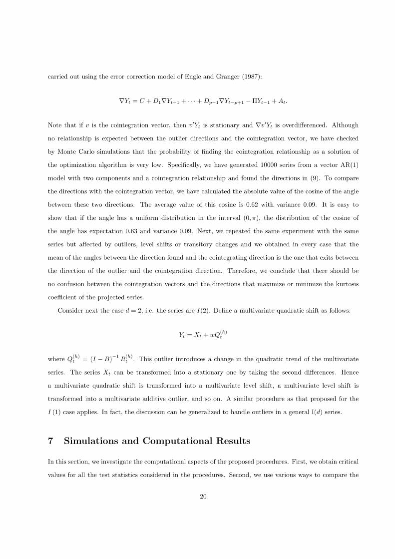
Table 7: Estimation of the sizes of the ouliers detected by the algorithm.

Time Type w1(t−ratio)

w2(t−ratio)

w3(t−ratio)

1966 MLS 0.0165(1.7046)

0.0473(7.0546)

0.0152(2.0114)

1975 MRS −0.0167(−1.9723)

−0.0224(−2.4668)

−0.0196(−2.2817)

1975 MAO −0.0434(−1.8392)

−0.0672(−4.1121)

−0.0312(−1.6917)

Table 8: Summary of the procedure proposed in Tsay et al. (2000).

OutlierIterations (JI , hI) (JA, hA) (JL, hL) (JT , hT ) Time Type

1 (15.08,1966) (15.54,1965) (11.39,1975) (14.11,1966) — —2 (3.78,1966) (3.84,1965) (3.16,1975) (3.42,1966) — —

(.5S+.5F)-I, where S, F and I denote the log GNP of Spain, France and Italy, respectively. After outlier

modeling, the cointegration vector roughly becomes (.64S+.36F)-I, which gives heavier weight to the Spanish

GNP.

Finally, we compare the results with those obtained by applying the procedure of Tsay et al. (2000).

The critical values for the multivariate statistics considered are 17.3 for MIO, MAO, and MTC, and 14.8 for

MLS. The critical values for the component statistics are 3.9 for MIO, MAO and MTC and 3.6 for MLS.

Table 8 summarizes the results using the same first-order vector error correction model. The procedure fails

to detect any outliers.

9 Appendix: Proofs

Proof of Lemma 1. The kurtosis of yt can be written as:

γy (v) = E

1

n

n∑t=1

(yt − 1

n

n∑

l=1

yl

)4 =

1n

n∑t=1

E

(yt − 1

n

n∑

l=1

yl

)4 .

29

As yt = xt + r(h,n)t and taking into account that xt and r

(h,n)t are independent and E [xt] = E

[x3

t

]= 0, we

get

E

(yt − 1

n

n∑

l=1

yl

)4 = E

[(xt + rt − r)4

]= E

[x4

t

]+ 6E

[x2

t

](rt − r)2 + (rt − r)4 ,

and

γy (v) =1n

n∑t=1

(E

[x4

t

]+ 6E

[x2

t

](rt − r)2 + (rt − r)4

)

=1n

n∑t=1

E[x4

t

]+

6n

n∑t=1

E[x2

t

](rt − r)2 +

1n

n∑t=1

(rt − r)4 .

Finally, as E[x2

t

]= v′v, E

[x4

t

]= 3E

[x2

t

]2 = 3 (v′v)2, 1n

∑nt=1 (rt − r)2 = v′ΣRv and v′v = v′ΣY v −

v′ΣRv, we obtain

γy (v) = 3 (v′ΣY v)2 − 3 (v′ΣRv)2 + ωr (v) .

Proof of Lemma 2. The Lagrangian for the extreme points of γy (v) is

£ (v) = 3− 3 (v′ΣRv)2 + ωr (v)− λ (v′ΣY v − 1) ,

and its gradient is

∇£ (v) = −12 (v′ΣRv)ΣRv +

(4n

n∑t=1

(rt − r)2 Bt

)v − 2λΣY v = 0.

Multiplying by v′ in∇£ (v) and taking into account the constraint v′ΣY v = 1, we have λ = −6 (v′ΣRv)2+

2ωr (v). As ΣR = 1n

∑nt=1 Bt, then

−12 (v′ΣRv)ΣRv + 4

(1n

n∑t=1

(v′Btv) Bt

)v =

(−12 (v′ΣRv)2 +

4n

n∑t=1

(v′Btv)2)

(I + ΣR)v.

30

Therefore,

−3 (v′ΣRv) ΣRv + 3 (v′ΣRv)2 ΣRv +

(1n

n∑t=1

(v′Btv) Bt

)v − 1

n

n∑t=1

(v′Btv)2 ΣRv

= −3 (v′ΣRv)2 v +1n

n∑t=1

(v′Btv)2 v,

and, finally,n∑

t=1

[(v′Btv)− 3 (v′ΣRv)− µ (v)

n

]Btv = n (v′ΣRv)2 (γr (v)− 3) v.

This implies that the extreme directions of £ (v) under the constraint v′ΣY v = 1 are the eigenvectors of

the matrix [n∑

t=1

βt (v)Bt

]v = µ (v) v,

where βt (v) =[(v′Btv)− 3 (v′ΣRv)− µ(v)

n

]and µ (v) = n (v′ΣRv)2 (γr (v)− 3). From (8), we get that:

γy (v) = 3− σ4r (3− γr (v)) = 3 +

µ (v)n

.

Therefore, the maximum or the minimum of γy (v) will be given when µ (v) is as large or as small as

possible respectively, and the maximum and the minimum of the kurtosis will be given by the maximum and

the minimum of the eigenvalues of the matrix∑n

t=1 βt (v) Bt.

Proof of Theorem 3. In the proof, we use the following equalities:

v′ΣRv =1n

n∑t=1

(rt − r)2 , v′Btv = (rt − r)2 , (v′ΣRv)2 γr (v) =1n

n∑t=1

(rt − r)4 ,

where r = 1n

∑nt=1 rt.

1. In the MAO case, rh = v′w, rt = 0, ∀t 6= h and r = 1nrh. First, n (v′ΣRv)2 γr (v) = c1r

4h and

v′ΣRv = c2r2h, where

c1 =(

1− 1n

) [(1− 1

n

)3

+1n3

], c2 =

1n

(1− 1

n

),

31

and consequently, the eigenvalues are given by µ (v) = c0r4h, where

c0 = c1 − 3nc22 =

(1− 1

n

)[1− 6

n

(1− 1

n

)].

On the other hand, after some algebra it can be shown that

[n∑

t=1

βt (v)Bt

]v =

[m1r

3h + m2r

5h

]Rh,

where

m1 =(

1− 1n

) [1n3

+(

1− 1n

)3

− 3c2

], m2 = −c0

1n

(1− 1

n

).

As Rh = w,

v =m1r

3h + m2r

5h

c0r4h

w,

and the other eigenvectors are orthogonal to w. Moreover, as the eigenvalues are given by c0r4h and

c0 > 0 for n > 5, we get that the maximum of the kurtosis coefficient is given in the direction of w,

while the minimum is attained in the orthogonal directions to w.

2. In the MTC case, rt = 0 if t < h, rt = δt−hrh for t ≥ h and r = mrh, where m =(1− δn−h+1

)/ (n (1− δ)).

First, n (v′ΣRv)2 γr (v) = c1r4h and v′ΣRv = c2r

2h, where

c1 = (h− 1) m4 +n∑

t=h

(δt−h −m

)4, c2 =

1n

[(h− 1) m2 +

n∑

t=h

(δt−h −m

)2

],

and consequently, the eigenvalues are given by µ (v) = c0r4h, where c0 = c1− 3nc2

2. On the other hand,

after some algebra, it can be shown that

[n∑

t=1

βt (v)Bt

]v =

[m1r

3h + m2r

5h

]Rh,

where

m1 = (h− 1)(m4 − 3c2m

2)

+n∑

t=h

[(δt−h −m

)4 − 3c2

(δt−h −m

)2]

m2 = −c0

n

[(h− 1)m2 +

n∑

t=h

(δt−h −m

)2

],

32

and, consequently, one eigenvector is proportional to w and the others are orthogonal to it. As the

eigenvalues are given by c0r4h, the kurtosis coefficient of yt is maximized or minimized when v is

proportional to w depending on the sign of c0, that in general depends on the values of n, h and δ.

3. In the MLS case, rt = 0 if t < h, rt = rh for t ≥ h and r = n−h+1n rh. First, n (v′ΣRv)2 γr (v) = c1r

4h and

v′ΣRv = c2r2h, where

c1 =(h− 1) (n− h + 1)

n4

[(n− h + 1)3 + (h− 1)3

], c2 =

(h− 1) (n− h + 1)n2

,

and consequently, the eigenvalues are given by µ (v) = c0r4h, where

c0 = c1 − 3nc22 =

(h− 1) (n− h + 1)n3

[n2 − 6n (h− 1) + 6 (h− 1)2

].

On the other hand, after some algebra, it can be shown that

[n∑

t=1

βt (v)Bt

]v =

[m1r

3h + m2r

5h

]Rh,

where

m1 =(h− 1) (n− h + 1)

n4

[(n− h + 1)3 + (h− 1)3 − 3c2

]m2 = −c0

(h− 1) (n− h + 1)n2

showing that one eigenvector is proportional to w and the others are orthogonal to it. The eigenvalues

are given by c0r4h and it is not difficult to see that

c0 < 0 ⇐⇒ h ∈(

1 +12

(1− 1√

3

)n, 1 +

12

(1 +

1√3

)n

)

c0 > 0 ⇐⇒ h /∈(

1 +12

(1− 1√

3

)n, 1 +

12

(1 +

1√3

)n

).

Therefore the maximum of the kurtosis coefficient is given in the direction of w if c0 > 0 and the

minimum of the kurtosis coefficient is given in the direction of w if c0 < 0.

Proof of Corollary 4. The result follows immediately from Theorem 3, because the relation At =

Et + wI(h)t coincides with the MAO case in a white noise series.

33

REFERENCES

Bai, J. (1994) “Least Squares Estimation of a Shift in linear processes”, Journal of Time Series Analysis,

15, 453-472.

Balke, N. S. (1993) “Detecting level shifts in time series”, Journal of Business and Economic Statistics, 11,

81-92.

Bianco, A. M., Garcia Ben, M., Martınez, E. J. and Yohai, V. J. (2001) “Outlier Detection in Regression

Models with ARIMA Errors using Robust estimates”, Journal of Forecasting, 20, 565-579.

Billingsley, P. (1968) Convergence of Probability Measures, John Wiley & Sons.

Carnero, M. A., Pena, D. and Ruiz, E. (2003) “Detecting level shifts in the presence of conditional het-

erokedasticity” Technical Report, Universidad Carlos III de Madrid.

Chang I. and Tiao G. C. (1983) “Estimation of Time Series Parameters in the Presence of Outliers”

Technical Report 8, Statistics Research Center, University of Chicago.

Chang I., Tiao, G. C. and Chen, C. (1988) “Estimation of Time Series Parameters in the Presence of

Outliers”, Technometrics, 3, 193-204.

Chen, C. and Liu, L. (1993) “Joint Estimation of Model Parameters and Outlier Effects in Time Series”,

Journal of the American Statistical Association, 88, 284-297.

Engle, R. and Granger, C. W. J. (1987) “Co-integration and Error Correction: Representation, Estimation,

and Testing”, Econometrica, 55, 251-276.

Fox, A. J. (1972) “Outliers in Time Series”, Journal of the Royal Statistical Society B, 34, 350-363.

Huber, P. (1985) “Projection Pursuit (with discussion)”, The Annals of Statistics, 13, 435-525.

Inclan, C. and Tiao, G. C. (1994) “Use of Cumulative Sums of Squares for Retrospective Detection of

Changes of Variance”, Journal of the American Statistical Association, 89, 913-923.

Johansen, S. (1991) “Estimation and Hypothesis Testing of Cointegration Vectors in Gaussian Vector

Autoregressive Models”, Econometrica, 59, 1551-1580.

Jones, M. C. and Sibson, R. (1987) “What is Projection Pursuit (with discussion)?”, Journal of the Royal

Statistical Society A, 150, 1-36.

34

Justel, A., Pena, D. and Tsay, R. S. (2000) “Detection of Outlier Patches in Autoregressive Time Series”,

Statistica Sinica, 11, 651-673.

Le, N. D., Martin, R. D. and Raftery, A. E. (1996) “Modeling flat stretches, bursts, and outliers in time

series using mixture transition distribution models”, Journal of the American Statistical Association,

91, 1504-1515.

Luceno, A. (1998) “Detecting possibly non-consecutive outliers in industrial time series”, Journal of the

Royal Statistical Society B, 60, 295-310.

Lutkepohl, H. (1993) Introduction to Multiple Time Series Analysis, 2nd Ed., New York: Springer-Verlag.

McCulloch, R. E. and Tsay, R. S. (1993). “Bayesian inference and prediction for mean and variance shifts

in autoregressive time series”, Journal of the American Statistical Association, 88, 968–978.

McCulloch, R. E. and Tsay, R. S. (1994). “Bayesian analysis of autoregressive time series via the Gibbs

sampler” Journal of Time Series Analysis, 15, 235–250.

Maravall, A. and Mathis, A. (1994) “Encompassing univariate models in multivariate time series”, Journal

of Econometrics, 61, 197-233.

Pena, D. and Prieto, F. J. (2001, a) “Multivariate Outlier Detection and Robust Covariance Matrix Esti-

mation (with discussion)”, Technometrics, 43, 286-310.

Pena, D. and Prieto, F. J. (2001, b) “Cluster Identification Using Projections”, Journal of the American

Statistical Association, 96, 1433-1445.

Posse, C. (1995) “Tools for two-dimensional exploratory projection pursuit”, Journal of Computational and

Graphics Statistics, 4, 83-100.

Priestley, M. B. (1981) Spectral Analysis and Time Series, London: Academic Press.

Rao, C. R. (1973) Linear Statistical Inference and Its Applications, New York: John Wiley & Sons.

Sanchez, M. J. and Pena, D. (2003), “The identification of Multiple Outliers in ARIMA models”, Commu-

nications in Statistics: Theory and Methods, 32, 1265-1287.

Tsay, R. S. (1986) “Time Series Model Specification in the Presence of Outliers”, Journal of the American

Statistical Association, 81, 132-141.

35

Tsay, R. S. (1988) “Outliers, level shifts and variance changes in time series”, Journal of Forecasting, 7,

1-20.

Tsay, R. S., Pena, D. and Pankratz, A.E. (2000) “Outliers in Multivariate Time Series”, Biometrika, 87,

789-804.

36