Out-of-plane shape determination in generalized fringe projection profilometry

Out-of-plane shape determination ingeneralized fringe projection

profilometry

Zhaoyang Wang, Hua DuDepartment of Mechanical Engineering, The Catholic University of America,

Washington, DC 20064

[email protected], [email protected]

Hongbo BiDepartment of Mechanical Engineering, University of Maryland,

College Park, MD 20742

[email protected]

Abstract: The out-of-plane shape determination in a generalizedfringe projection profilometry is presented. The proposed techniquecorrects the problems in existing approaches, and it can cope well withthe divergent illumination encountered in the generalized profilometry.In addition, the technique can automatically detect the geometric para-meters of the experimental setup, which makes the generalized fringeprojection profilometry simple and practical. The concept was verified byboth computer simulations and actual experiments. The technique can beeasily employed for out-of-plane shape measurements with high accuracies.

© 2006 Optical Society of America

OCIS codes: (120.2830) Height measurements; (120.6650) Surface measurements, figure;(120.6660) Surface measurements, roughness; (150.6910) Three-dimensional sensing

References and links1. K. Creath and J. Wyant, “Moire and fringe projection techniques,” in. Optical Shop Testing, 2nd Ed., Ed. by D.

Malacara, New York: Wiley, 653–685 (1992).2. F. Chen, G. Brown, and M. Song, “Overview of 3-D shape measurement using optical methods,” Opt. Eng. 39,

10–22 (2000).3. M. Takeda and K. Mutoh, “Fourier transform profilometry for the automatic measurement of 3-D object shapes,”

Appl. Opt. 22, 3977–3982 (1983).4. V. Srinivasan, H. Liu, and M. Halioua, “Automated phase-measuring profilometry of 3-D diffuse objects,” Appl.

Opt. 23, 3105–3108 (1984).5. V. Srinivasan, H. Liu, and M. Halioua, “Automated phase-measuring profilometry: a phase mapping approach,”

Appl. Opt. 24, 185–188 (1985).6. P. Huang, Q. Hu, F. Jin, and F. Chiang, “Color-encoded digital fringe projection technique for high-speed three-

dimensional surface contouring,” Opt. Eng. 38, 1065–1071 (1999).7. W. Schreiber and G. Notni, “Theory and arrangements of self-calibrating whole-body three-dimensional

measurement systems using fringe projection technique,” Opt. Eng. 39, 159-169 (2000).8. L. Salas, E. Luna, J. Salinas, V. Garcia, and M. Servin, “Profilometry by fringe projection,” Opt. Eng. 42, 3307–

3314 (2003).9. C. Quan, C. Tay, X. Kang, X. He, and H. Shang, “Shape measurement by use of liquid-crystal display fringe

projection with two-step phase shifting,” Appl. Opt. 42, 2329–2335 (2003).10. C. Tay, C. Quan, H. Shang, T. Wu, and S. Wang, “New method for measuring dynamic response of small com-

ponents by fringe projection,” Opt. Eng. 42, 1715-1720 (2003).

#76499 - $15.00 USD Received 27 October 2006; accepted 28 November 2006

(C) 2006 OSA 11 December 2006 / Vol. 14, No. 25 / OPTICS EXPRESS 12122

11. C. Tay, C. Quan, T. Wu, and Y. Huang, “Integrated method for 3-D rigid-body displacement measurement usingfringe projection,” Opt. Eng. 43, 1152-1159 (2004).

12. J. Pan, P. Huang, and F. Chiang, “Color-coded binary fringe projection technique for 3-D shape measurement,”Opt. Eng. 44,, 023606 (2005).

13. H. Guo, H. He, Y. Yu, and M. Chen, “Least-squares calibration method for fringe projection profilometry,” Opt.Eng. 44, 033603, (2005).

14. L. Chen and C. Quan, “Fringe projection profilometry with nonparallel illumination : a least-squares approach,”Opt. Lett. 30, 2101–2103 (2005).

15. Z. Wang and H. Bi, “Comment on ”Fringe projection profilometry with nonparallel illumination: a least-squaresapproach”,” Opt. Lett. 31, 1972–1973 (2006).

16. L. Chen and C. Quan, “Reply to Comment on ”Fringe projection profilometry with nonparallel illumination: aleast-squares approach”,” Opt. Lett. 31, 1974–1975 (2006).

17. Z. Wang and B. Han, “Advanced iterative algorithm for phase extraction of randomly phase-shifted interfero-grams,” Opt. Lett. 29, 1671–1673 (2004).

18. Z. Wang, “Development and application of computer-aided fringe analysis,” Ph.D. Dissertation, University ofMaryland at College Park, 2003. htt p : //hdl.handle.net/1903/31

1. Introduction

Fringe projection profilometry has been well established for out-of-plane shape and warpagemeasurements [1]- [16]. In the conventional fringe projection profilometry [1], a collimatedlight beam is employed to project straight and equally spaced fringes on a specimen, and theimages of the specimen and the projected fringes are captured from a different direction otherthan the illumination direction. The departure of a viewed fringe on the specimen from a straightline contains information of the departure of the specimen surface from the reference surface,i.e., the out-of-plane height (shape or warpage). Generally, the out-of-plane shape or warpageis obtained through extracting the relevant phase distributions from the projected fringes.

In recent years, digital LCD or DLP projectors, due to their multiple advantages such asconvenience and low cost, have been widely used in fringe projection profilometry for out-of-plane shape or warpage measurements. In practice, although the projector-based techniqueis relatively easy to implement, the measurement accuracy is subjected to uncertainties in thesystem. These uncertainties can further cause substantial errors in shape or warpage deter-minations. Specifically, the primary uncertainty originates from the divergent or uncollimatedillumination which not only induces nonlinearities to the reference carriers but also makes anaccurate determination of the out-of-plane height difficult. In addition, the techniques based ondivergent projection normally require specific and precise experimental setups, but the geomet-ric parameters such as the projection angle and the location of the focal point of projector lensare quite difficult to determine precisely. In existing techniques [3]- [13], these uncertainties aregenerally more or less neglected, thus the corresponding measurement accuracies are inevitablydiminished.

To cope with the nonlinear carrier problem, a number of approaches have been proposed.A typical scheme is capturing the images of reference plane and test object separately to ob-tain the full-field fringe phase maps [5] [13]. However, this handling is inconvenient in actualapplication; moreover, because the distributions of carrier fringe pitches remain unknown, theout-of-plane height determination is only an approximation . Recently, Chen et al. [14]- [16]described a least-squares approach to determine the nonlinear carrier phases with a polynomialfunction, and their algorithm is very effective for the reference carrier detection under nonpar-allel illumination. In spite of the advances in the carrier phase detection, it is noted that a cor-responding technique to accurately determine the out-of-plane height is lacking. The existingalgorithms either rely on a precise experimental setup which is impractical to achieve or simplyuse a phase-subtraction scheme. It is important to point out that the algorithms based on a directsubtraction of carrier phases from the projection fringe phases, which is originally employedfor parallel or collimated illumination case, have been extended and applied to projector-based



profilometry in the literatures [9]- [12]. However, the algorithms based on phase-subtraction arenot theoretically rigorous for the case of divergent illumination. Due to above reasons, the ex-isting techniques normally provide the out-of-plane shape approximately instead of accurately.

Other notable works include a self-calibrating system developed by Schreiber et al. [7] and amultiple-parameters technique introduced by Salas et al. [8] for carrier subtraction and heightdetection. These two techniques are very complicated and subjected to errors due to manualintervention, which makes the techniques impractical.

In this paper, a mathematical derivation of the carrier phase function for fringe projectionprofilometry with divergent illumination is presented, and a rigorous algorithm to determinethe out-of-plane shape for a generalized fringe projection profilometry is proposed. The pro-posed technique allows using a conventional projector (i.e., the illumination is divergent) inthe experiment; furthermore, it neither requires a specific and precise experimental setup norrequires the geometric parameters of experimental setup to be measured. The technique is ca-pable of quickly providing out-of-plane shape and warpage measurements with high accuraciesfor the generalized fringe projection profilometry with divergent illuminations.

2. Principle

2.1. Experimental setup

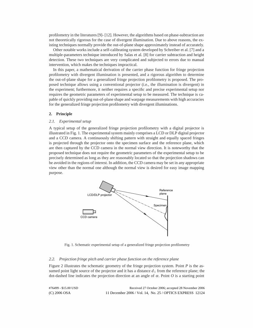
A typical setup of the generalized fringe projection profilometry with a digital projector isillustrated in Fig. 1. The experimental system mainly comprises a LCD or DLP digital projectorand a CCD camera. A continuously shifting pattern with straight and equally spaced fringesis projected through the projector onto the specimen surface and the reference plane, whichare then captured by the CCD camera in the normal view direction. It is noteworthy that theproposed technique does not require the geometric parameters of the experimental setup to beprecisely determined as long as they are reasonably located so that the projection shadows canbe avoided in the regions of interest. In addition, the CCD camera may be set in any appropriateview other than the normal one although the normal view is desired for easy image mappingpurpose.

CCD camera

LCD/DLP projector

Specimen

Reference plane

Fig. 1. Schematic experimental setup of a generalized fringe projection profilometry

2.2. Projection fringe pitch and carrier phase function on the reference plane

Figure 2 illustrates the schematic geometry of the fringe projection system. Point P is the as-sumed point light source of the projector and it has a distance d 1 from the reference plane; thedot-dashed line indicates the projection direction at an angle of α . Point O is a starting point



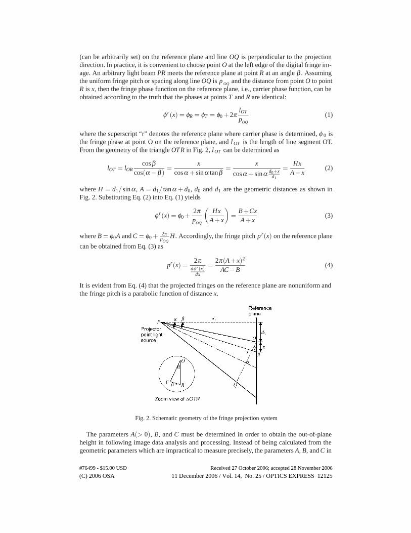
(can be arbitrarily set) on the reference plane and line OQ is perpendicular to the projectiondirection. In practice, it is convenient to choose point O at the left edge of the digital fringe im-age. An arbitrary light beam PR meets the reference plane at point R at an angle β . Assumingthe uniform fringe pitch or spacing along line OQ is p OQ and the distance from point O to pointR is x, then the fringe phase function on the reference plane, i.e., carrier phase function, can beobtained according to the truth that the phases at points T and R are identical:

φ r(x) = φR = φT = φ0 +2πlOT

pOQ

(1)

where the superscript “r” denotes the reference plane where carrier phase is determined, φ 0 isthe fringe phase at point O on the reference plane, and l OT is the length of line segment OT.From the geometry of the triangle OTR in Fig. 2, lOT can be determined as

lOT = lORcosβ

cos(α −β )=

xcosα + sinα tanβ

=x

cosα + sinα d0+xd1

=Hx

A+ x(2)

where H = d1/sinα , A = d1/ tanα + d0, d0 and d1 are the geometric distances as shown inFig. 2. Substituting Eq. (2) into Eq. (1) yields

φ r(x) = φ0 +2πpOQ

(Hx

A+ x

)=

B+CxA+ x

(3)

where B = φ0A and C = φ0 + 2πpOQ

H. Accordingly, the fringe pitch pr(x) on the reference plane

can be obtained from Eq. (3) as

pr(x) =2π

dφ r(x)dx

=2π(A+ x)2

AC−B(4)

It is evident from Eq. (4) that the projected fringes on the reference plane are nonuniform andthe fringe pitch is a parabolic function of distance x.

Fig. 2. Schematic geometry of the fringe projection system

The parameters A(> 0), B, and C must be determined in order to obtain the out-of-planeheight in following image data analysis and processing. Instead of being calculated from thegeometric parameters which are impractical to measure precisely, the parameters A, B, and C in



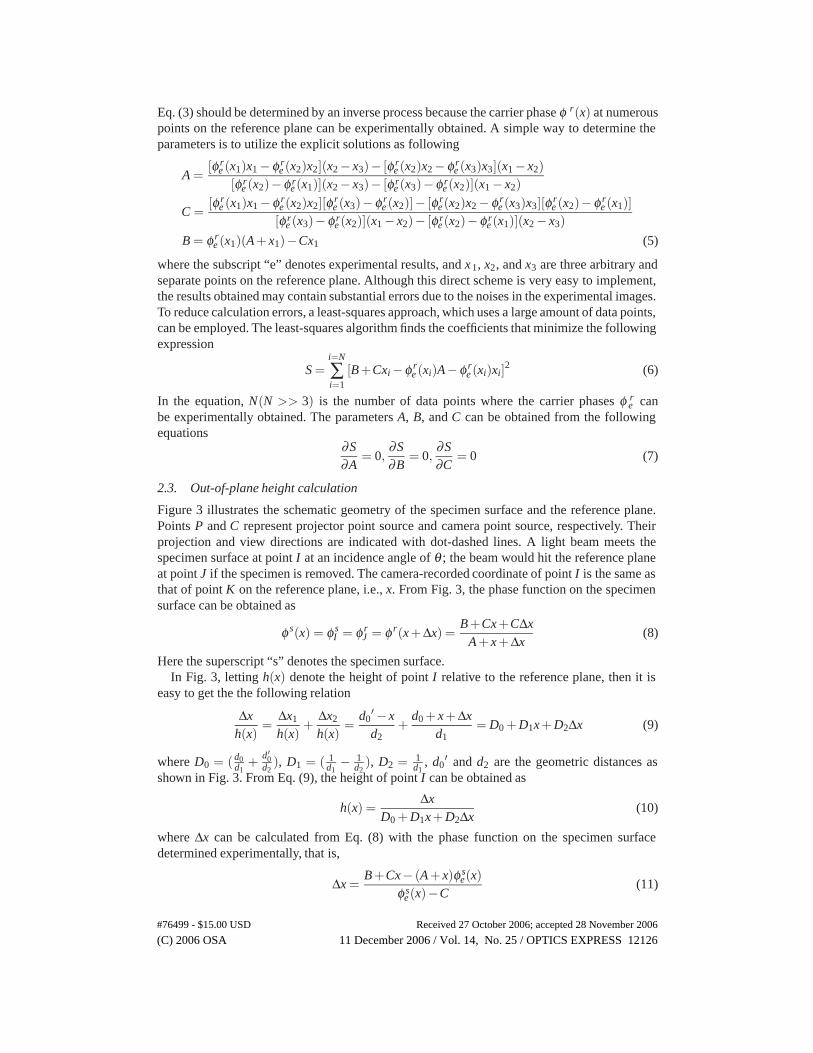
Eq. (3) should be determined by an inverse process because the carrier phase φ r(x) at numerouspoints on the reference plane can be experimentally obtained. A simple way to determine theparameters is to utilize the explicit solutions as following

A =[φ r

e (x1)x1 −φ re (x2)x2](x2 − x3)− [φ r

e (x2)x2 −φ re (x3)x3](x1 − x2)

[φ re (x2)−φ r

e (x1)](x2 − x3)− [φ re (x3)−φ r

e (x2)](x1 − x2)

C =[φ r

e (x1)x1 −φ re (x2)x2][φ r

e (x3)−φ re (x2)]− [φ r

e (x2)x2 −φ re (x3)x3][φ r

e (x2)−φ re (x1)]

[φ re (x3)−φ r

e (x2)](x1 − x2)− [φ re (x2)−φ r

e (x1)](x2 − x3)B = φ r

e (x1)(A+ x1)−Cx1 (5)

where the subscript “e” denotes experimental results, and x1, x2, and x3 are three arbitrary andseparate points on the reference plane. Although this direct scheme is very easy to implement,the results obtained may contain substantial errors due to the noises in the experimental images.To reduce calculation errors, a least-squares approach, which uses a large amount of data points,can be employed. The least-squares algorithm finds the coefficients that minimize the followingexpression

S =i=N

∑i=1

[B+Cxi−φ re (xi)A−φ r

e (xi)xi]2 (6)

In the equation, N(N >> 3) is the number of data points where the carrier phases φ re can

be experimentally obtained. The parameters A, B, and C can be obtained from the followingequations

∂S∂A

= 0,∂S∂B

= 0,∂S∂C

= 0 (7)

2.3. Out-of-plane height calculation

Figure 3 illustrates the schematic geometry of the specimen surface and the reference plane.Points P and C represent projector point source and camera point source, respectively. Theirprojection and view directions are indicated with dot-dashed lines. A light beam meets thespecimen surface at point I at an incidence angle of θ ; the beam would hit the reference planeat point J if the specimen is removed. The camera-recorded coordinate of point I is the same asthat of point K on the reference plane, i.e., x. From Fig. 3, the phase function on the specimensurface can be obtained as

φ s(x) = φ sI = φ r

J = φ r(x+ Δx) =B+Cx+CΔx

A+ x+ Δx(8)

Here the superscript “s” denotes the specimen surface.In Fig. 3, letting h(x) denote the height of point I relative to the reference plane, then it is

easy to get the the following relation

Δxh(x)

=Δx1

h(x)+

Δx2

h(x)=

d0′ − xd2

+d0 + x+ Δx

d1= D0 +D1x+D2Δx (9)

where D0 = ( d0d1

+ d′0d2

), D1 = ( 1d1

− 1d2

), D2 = 1d1

, d0′ and d2 are the geometric distances as

shown in Fig. 3. From Eq. (9), the height of point I can be obtained as

h(x) =Δx

D0 +D1x+D2Δx(10)

where Δx can be calculated from Eq. (8) with the phase function on the specimen surfacedetermined experimentally, that is,

Δx =B+Cx− (A+ x)φ s

e(x)φ s

e (x)−C(11)



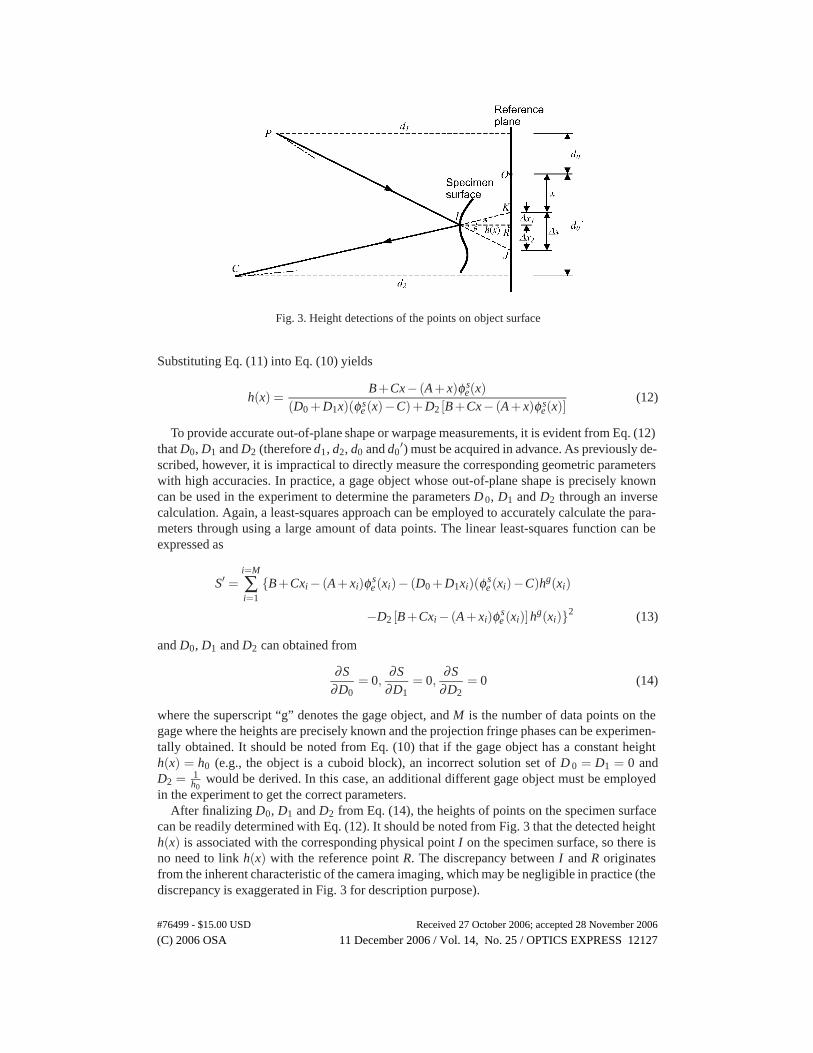
Fig. 3. Height detections of the points on object surface

Substituting Eq. (11) into Eq. (10) yields

h(x) =B+Cx− (A+ x)φ s

e(x)(D0 +D1x)(φ s

e (x)−C)+D2 [B+Cx− (A+ x)φ se(x)]

(12)

To provide accurate out-of-plane shape or warpage measurements, it is evident from Eq. (12)that D0, D1 and D2 (therefore d1, d2, d0 and d0

′) must be acquired in advance. As previously de-scribed, however, it is impractical to directly measure the corresponding geometric parameterswith high accuracies. In practice, a gage object whose out-of-plane shape is precisely knowncan be used in the experiment to determine the parameters D 0, D1 and D2 through an inversecalculation. Again, a least-squares approach can be employed to accurately calculate the para-meters through using a large amount of data points. The linear least-squares function can beexpressed as

S′ =i=M

∑i=1

{B+Cxi− (A+ xi)φ se (xi)− (D0 +D1xi)(φ s

e (xi)−C)hg(xi)

−D2 [B+Cxi− (A+ xi)φ se (xi)]hg(xi)}2 (13)

and D0, D1 and D2 can obtained from

∂S∂D0

= 0,∂S

∂D1= 0,

∂S∂D2

= 0 (14)

where the superscript “g” denotes the gage object, and M is the number of data points on thegage where the heights are precisely known and the projection fringe phases can be experimen-tally obtained. It should be noted from Eq. (10) that if the gage object has a constant heighth(x) = h0 (e.g., the object is a cuboid block), an incorrect solution set of D 0 = D1 = 0 andD2 = 1

h0would be derived. In this case, an additional different gage object must be employed

in the experiment to get the correct parameters.After finalizing D0, D1 and D2 from Eq. (14), the heights of points on the specimen surface

can be readily determined with Eq. (12). It should be noted from Fig. 3 that the detected heighth(x) is associated with the corresponding physical point I on the specimen surface, so there isno need to link h(x) with the reference point R. The discrepancy between I and R originatesfrom the inherent characteristic of the camera imaging, which may be negligible in practice (thediscrepancy is exaggerated in Fig. 3 for description purpose).



3. Simulation

A computer simulation was implemented to verify the validity of the proposed algorithm. Theprojection fringe image used in the simulation is shown in Fig. 4, which represents a partialsphere of peak height 10.72mm and curvature of 0.0125mm −1, a cuboid gage block of height10mm, and another cuboid gage block of height 20mm on a flat surface. The fringe patternsin Fig. 4 were generated according to the geometric relations of a divergent illumination setup,and the conventional four-frame phase shifting concept was adopted to obtain four phase-shiftedimages in the simulation. The non-uniformity of the projection fringes due to divergent illumi-nation is evident in the figure.

Fig. 4. Computer-generated projection fringe patterns

As a comparison, two existing techniques, in addition to the proposed one, were incorporatedin the simulation:

1. A conventional technique which was originally developed for parallel or collimated illu-mination case. Since the algorithm has been used in divergent illumination application, itwas investigated in the simulation.

2. A polynomial technique which utilizes a polynomial function to describe the carrierphase [14] [16]. It is the best technique among existing ones for carrier phase detection.

For both techniques, the most widely used phase-subtraction algorithm [4], [9]- [12], [14] isemployed for the determination of the out-of-plane heights. Table 1 summarizes the techniquesincorporated.

Table 1. Comparison of the techniques

Technique Carrier phase function Out-of-plane height functionConventional φ = Ax+B h(x) = k[φ s(x)−φ r(x)]Polynomial φ = A0 +A1x+A2x2 + ... h(x) = k[φ s(x)−φ r(x)]Proposed φ = B+Cx

A+x h(x) = B+Cx−(A+x)φ se(x)

(D0+D1x)(φ se (x)−C)+D2[B+Cx−(A+x)φ s

e (x)]

The out-of-plane shapes obtained from the three different techniques are shown in Fig. 5. Ineach figure, the results have been normalized to demonstrate the relative heights. It is easy to seefrom the figure that the proposed technique can detect the out-of-plane shape more accuratelythan the existing techniques. Figure 6 shows a comparison of the absolute height values (withthe flat surface as the reference plane) along the horizontal centerlines in the images. It is notedthat the coefficients k in the relevant governing equations of the conventional and polynomialalgorithms were intentionally set to specific values so that the detected average height of thesecond cuboid block is identical with the theoretical height of 20mm. From Fig. 6, it is evidentthat the results obtained from the proposed technique exactly match the theoretical heights,



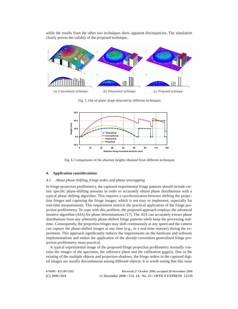
while the results from the other two techniques show apparent discrepancies. The simulationclearly proves the validity of the proposed technique.

(a) Conventional technique (b) Polynomial technique (c) Proposed technique

Fig. 5. Out-of-plane shape detected by different techniques

-10.0

0.0

10.0

20.0

30.0

0 16 32 48 64 80 96 112 128Distance along horizontal direction (mm)

Hei

ght (

mm

)

TheoreticalConventionalPolynomialProposed

Fig. 6. Comparisons of the absolute heights obtained from different techniques

4. Application considerations

4.1. About phase shifting, fringe order, and phase unwrapping

In fringe projection profilometry, the captured experimental fringe patterns should include cer-tain specific phase-shifting amounts in order to accurately obtain phase distributions with atypical phase shifting algorithm. This requires a synchronization between shifting the projec-tion fringes and capturing the fringe images, which is not easy to implement, especially forreal-time measurements. This requirement restricts the practical application of the fringe pro-jection profilometry. To cope with this problem, the proposed approach employs the advancediterative algorithm (AIA) for phase determinations [17]. The AIA can accurately extract phasedistributions from any arbitrarily phase-shifted fringe patterns while keep the processing real-time. Consequently, the projection fringes may shift continuously at any speed and the cameracan capture the phase-shifted images at any time (e.g., in a real-time manner) during the ex-periment. This approach significantly reduces the requirements on the hardware and softwareimplementations and makes the application of the already-convenient generalized fringe pro-jection profilometry more practical.

A typical experimental image of the proposed fringe projection profilometry normally con-tains the images of the specimen, the reference plane and the calibration gage(s). Due to theexisting of the multiple objects and projection shadows, the fringe orders in the captured digi-tal images are usually discontinuous among different objects. It is worth noting that this issue



was not clearly addressed in previous work, thus the test object must have some surface pointscontact the reference plane to make the fringe orders continuous across the whole field [3]-[14]. Such a restriction highly limits the applicability of the fringe projection profilometry. Inthis paper, this practically important issue is easily resolved by adding one or more markers ineach valid and isolated region to indicate the relative fringe orders. An example of projectingfringe-order markers will be demonstrated in the following section.

Another problem associated with the isolated regions is that the phase unwrapping algorithmshould be able to simultaneously unwrap the phases and assign correct offsets to the phasesin multiple isolated areas. There are already several advanced phase unwrapping algorithms(e.g., PCG algorithm) available for such a task. An overview of the algorithms can be found inRef. [18].

4.2. About the calibration gage and the reference plane

The calibration gage(s) is useful for the detection of the governing parameters D 0, D1, and D2

required for the out-of-plane height determination without measuring the geometric parametersd0, d′

0, d1, and d2 of the experimental system. It is necessary to ensure that the gage height isaccurate enough to eliminate the influence on the measurement uncertainty. Once the governingparameters are finalized, the calibration gage(s) does not have to be included in the experimentsunless the corresponding geometric parameters have been changed.

The fringe projection profilometry provides the out-of-plane height measurements relativeto the reference plane. The reference plane is not necessarily the background plane and is notnecessarily located behind the objects of interest to be measured. Similar to the calibrationgage, the reference plane may be removed from the experimental setup once the parameters A,B, and C have been detected and unchanged.

5. Experiments

Two experiments have been conducted to demonstrate the applicability of the proposed tech-nique. One experiment intends to verify the measurement accuracy of the technique, and an-other one aims to show its practicability. The experimental procedure comprises the followingmajor steps:

1. Setup the reference plane, the calibration and test objects, the projection and camerasystems. It is preferable to set the projection at an inclined incidence angle and the cameraat a normal view with respect to the reference plane. There is no need to measure thegeometric parameters.

2. Shift the projection fringes continuously and capture a series of images. One image withfringe order markers, which are generated and controlled by the software, should becaptured as well.

3. Process the images to obtain the full-field out-of-plane shape. This step involves ex-tracting wrapped and unwrapped phases, offsetting fringe orders, detecting governingparameters, and determining height distributions.

5.1. Experiment one: accuracy examination

A cuboid block of nominal height 33.0mm was tested in the experiment for accuracy examina-tion. Figure 7 shows six experimental images with randomly phase-shifted projection fringes.In the images, the cuboid specimen can be found to the left of two gage blocks where the one indark gray is 50.8mm high and the white one is 36.5mm high. All the blocks are located againstthe background reference plane. From Fig. 7, it is clear that the illumination from the projectorto the objects and reference plane is uncollimated, and the fringe pitches have relatively largevariations across the field.



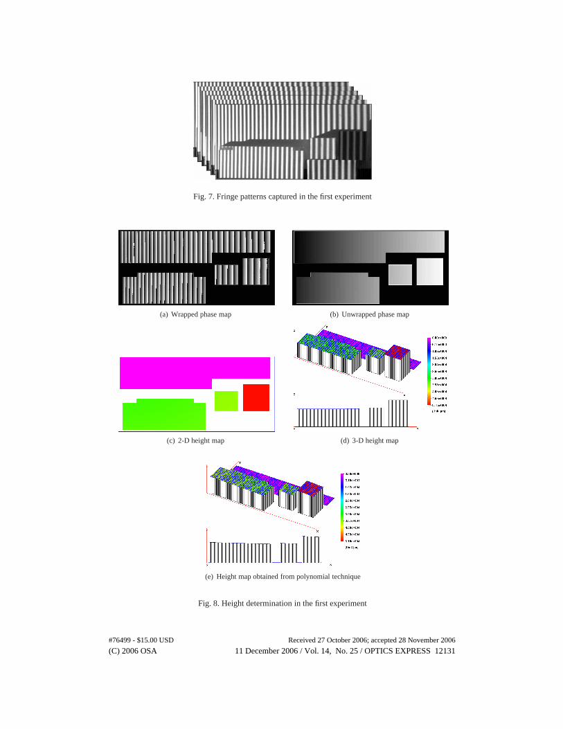
Fig. 7. Fringe patterns captured in the first experiment

(a) Wrapped phase map (b) Unwrapped phase map

(c) 2-D height map (d) 3-D height map

(e) Height map obtained from polynomial technique

Fig. 8. Height determination in the first experiment



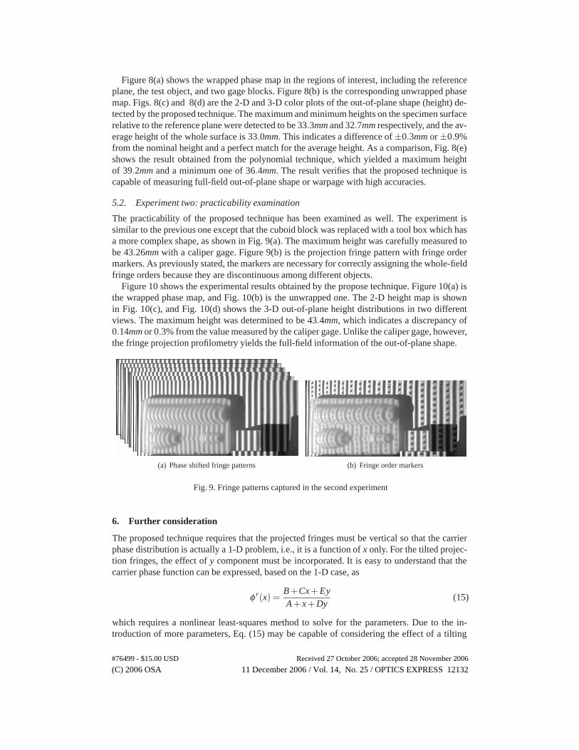
Figure 8(a) shows the wrapped phase map in the regions of interest, including the referenceplane, the test object, and two gage blocks. Figure 8(b) is the corresponding unwrapped phasemap. Figs. 8(c) and 8(d) are the 2-D and 3-D color plots of the out-of-plane shape (height) de-tected by the proposed technique. The maximum and minimum heights on the specimen surfacerelative to the reference plane were detected to be 33.3mm and 32.7mm respectively, and the av-erage height of the whole surface is 33.0mm. This indicates a difference of ±0.3mm or ±0.9%from the nominal height and a perfect match for the average height. As a comparison, Fig. 8(e)shows the result obtained from the polynomial technique, which yielded a maximum heightof 39.2mm and a minimum one of 36.4mm. The result verifies that the proposed technique iscapable of measuring full-field out-of-plane shape or warpage with high accuracies.

5.2. Experiment two: practicability examination

The practicability of the proposed technique has been examined as well. The experiment issimilar to the previous one except that the cuboid block was replaced with a tool box which hasa more complex shape, as shown in Fig. 9(a). The maximum height was carefully measured tobe 43.26mm with a caliper gage. Figure 9(b) is the projection fringe pattern with fringe ordermarkers. As previously stated, the markers are necessary for correctly assigning the whole-fieldfringe orders because they are discontinuous among different objects.

Figure 10 shows the experimental results obtained by the propose technique. Figure 10(a) isthe wrapped phase map, and Fig. 10(b) is the unwrapped one. The 2-D height map is shownin Fig. 10(c), and Fig. 10(d) shows the 3-D out-of-plane height distributions in two differentviews. The maximum height was determined to be 43.4mm, which indicates a discrepancy of0.14mm or 0.3% from the value measured by the caliper gage. Unlike the caliper gage, however,the fringe projection profilometry yields the full-field information of the out-of-plane shape.

(a) Phase shifted fringe patterns (b) Fringe order markers

Fig. 9. Fringe patterns captured in the second experiment

6. Further consideration

The proposed technique requires that the projected fringes must be vertical so that the carrierphase distribution is actually a 1-D problem, i.e., it is a function of x only. For the tilted projec-tion fringes, the effect of y component must be incorporated. It is easy to understand that thecarrier phase function can be expressed, based on the 1-D case, as

φ r(x) =B+Cx+EyA+ x+Dy

(15)

which requires a nonlinear least-squares method to solve for the parameters. Due to the in-troduction of more parameters, Eq. (15) may be capable of considering the effect of a tilting



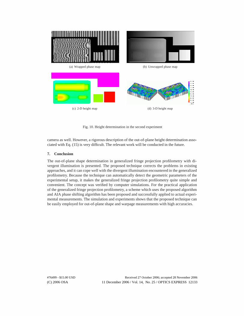
(a) Wrapped phase map (b) Unwrapped phase map

(c) 2-D height map (d) 3-D height map

Fig. 10. Height determination in the second experiment

camera as well. However, a rigorous description of the out-of-plane height determination asso-ciated with Eq. (15) is very difficult. The relevant work will be conducted in the future.

7. Conclusion

The out-of-plane shape determination in generalized fringe projection profilometry with di-vergent illumination is presented. The proposed technique corrects the problems in existingapproaches, and it can cope well with the divergent illumination encountered in the generalizedprofilometry. Because the technique can automatically detect the geometric parameters of theexperimental setup, it makes the generalized fringe projection profilometry quite simple andconvenient. The concept was verified by computer simulations. For the practical applicationof the generalized fringe projection profilometry, a scheme which uses the proposed algorithmand AIA phase shifting algorithm has been proposed and successfully applied to actual experi-mental measurements. The simulation and experiments shows that the proposed technique canbe easily employed for out-of-plane shape and warpage measurements with high accuracies.



Out-of-plane shape determination in generalized fringe projection profilometry

Documents