Systems GC28-0886-0 File No. S37Q-34 OS/VS2 MVS Performance Notebook Your performance hints, please ... This book will be updated as more information becomes available. You can submit performance hints for possible publication in this book. Use the reader's comment or Performance Notebook input formes) at the back of this book or send your information to: IBM Corporation Publications Department Department D58, Building 706-2 PO Box 390 Poughkeepsie, New York 12602 ATTN: Performance Notebook When submitting performance hints, see page iii for details. Li /

Welcome message from author
This document is posted to help you gain knowledge. Please leave a comment to let me know what you think about it! Share it to your friends and learn new things together.
Transcript

Systems
GC28-0886-0 File No. S37Q-34
OS/VS2 MVS Performance Notebook
Your performance hints, please ...
This book will be updated as more information becomes available. You can submit performance hints for possible publication in this book. Use the reader's comment or Performance Notebook input formes) at the back of this book or send your information to:
IBM Corporation Publications Department Department D58, Building 706-2 PO Box 390 Poughkeepsie, New York 12602 ATTN: Performance Notebook
When submitting performance hints, see page iii for details.
Li /
The recommendations given in this manual are based on experience with OS!VS2 MVS (Multiple Virtual Storage -. VS2 Release 3.7 with SUs 5 and 7 applied, and any subsequent VS2 releases) at internal IBM installations, at field test installations, and at user installations. As such, this material has not been submitted to any formal IBM test. Potential users should evaluate the applicability of the recommendations in their environment before implementation.
First Edition (July, 1977)
This edition applies to release 3.7 of OS/VS2 MVS and to all subsequent releases of MVS until otherwise indicated in new editions or Technical Newsletters. Changes may be made to the information herein; before using this publication in connection with the installation or operation of IBM systems, consult the latest IBM System/370 Bibliography, GC20-000 1, for the editions that are applicable and current.
Requests for copies of IBM publications should be made to your IBM representative or to the IBM branch office serving your locality.
A form for reader's comments is provided at the back of this publication. If the form has been removed, comments may be addressed to IBM Corporation, DepartmentD58, Building 706-2, PO Box 390, Poughkeepsie, New York 12602. Comments become the property of IBM.
© Copyright International Business Machines Corporation 1977
;' )

What To Expect From This Book
The subject of this book is performance evaluation: the process of tuning your system to meet your performance expectations and to optimize use of the system resources. There is no "cookbook" method to do a performance evaluation that will automatically provide you with specific performance solutions to apply to your system; the responsibility of identifying performance improvements for your system rests with you, the user. As a result, do not expect to find sure-fire performance solutions outlined in this book; there are no easy answers. Rather, this book attempts to provide necessary information for you to evaluate the performance of your system in a disciplined way, with some degree of confidence that the evaluation will succeed in identifying your system's problem areas and specific solutions for your particular installation.
The information is based on the experience of many MVS performance analysts. It is organized into the following sections:
• Introduction, which identifies the Significant problems that have frequently hampered performance evaluation and outlines the steps necessary to approach performance evaluation in a disciplined way.
• Part I, Planning and Preparing for a Performance Evaluation, which includes three chapters:
- Chapter 1.1, "Defining Performance Objectives," which describes factors you should include in defming what you expect from the system.
Chapter 1.2, "Selecting Measurement Tools," which provides an overview of tools available from IBM and describes other sources of MVS data.
Chapter 1.3, "Pre-initialization MVS Performance Factors," which outlines basic performance factors applicable to all system control programs, but which were often ignored in early experience with MVS systems.
• Part II, Performance Analysis, which documents a methodology for identifying potential problem areas in your system. The intent of this part is to help you focus on the area of most probable significant performance improvement in your system; the methodology is a combination of performance theory and MVS tuning experience. This part includes the following chapters:
Chapter 11.1, "Steps in a Performance Problem Analysis"
Chapter 11.2, "Investigating the Use of Processor Time"
Chapter 11.3, "Investigating the Use of I/O Resources"
Chapter 11.4, "Investigating the Use of Real Storage"
Chapter 11.5, "User-oriented Performance Problem Analysis"
iii

Chapters 11.2 -11.5 consist of background information that describes the general approach for investigating the resource or type of problem documented in the chapter, followed by bulletins that document specific areas to investigate and possible solutions to bottlenecks detected in those areas. The bulletins are numbered in the format x.y.O, where x represents the number of the chapter within Part II; y represents the number of the bulletin within the chapter; and ° allows for the addition of bulletins in future updates to this book.
Note that chapter 11.5 describes potential causes of delay that are also documented in the chapters on specific resources (for example, access to the processor; I/O delays; paging and swapping). The focus of chapter 11.5, however, differs from the focus in chapters 11.2 -11.4. In chapter 11.5, you are examining each resource in light of specific work that is not meeting its objective; in chapters 11.2-11.4, you are examining total usage of the resource.
• Part III, Performance Hints, which documents specific performance suggestions and considerations. This section is organized alphabetically by th~ topic of the hint. The choice of the title of each topic is somewhat arbitrary, in that many of the topics are related (for example, domain control hints and demand paging hints could also be considered SRM or real storage hints). We have tried to be as specific as possible in titling each topic and to avoid broad, general topics. The title page of Part III and the table of contents list the titles chosen for the· topiCS. In selecting hints to apply to your system, be sure they address a problem area identified in your system. The analysis documented in Part II should help you to identify problem areas.
The information in the book is based on a Release 3.7 MVS system with SUs 5 and 7 applied, unless otherwise indicated.
Although configuration planning and capacity planning are related to performance evaluation, they are not included in this book. They are addressed implicitly only to the extent that the analysis might help you to identify errors in configuration planning or the point at which additional capacity is. needed. This book also does not address benchmarking aspects of performance evaluation.
It is assumed that the user of this book is responsible for the performance evaluation of the installation's system; he or she should have experience in tuning complex systems and have a thorough knowledge of MVS concepts and facilities.
iv OS!VS2 MVS Performance Notebook

Submitting Performance Hints
This book will be updated as additional information becomes available. You can submit performance hints for possible publication in this book. Use the reader's comment or Performance Notebook input formes) at the back of this book or send your information to:
IBM Corporation Publications Department Department DS8, Building 706-2
. PO Box 390 Poughkeepsie, New York 12602 ATTN: Performance Notebook
It is understood that IBM and its affiliated companies shall have the nonexclusive right, in their discretion, to use, copy, and distribute all submitted information or material, in any form, for any and all purposes, without any obligation t9 the submitter, and that the submitter has the unqualified right to submit such information upon such basis.
When submitting performance hints, indicate the system and release level of your system and the SUs installed on your system.
Associated Publications and Selectable Units
The publications listed below are referenced in the text of this book. References in the book usually use an abbreviated form of the title and do not include the order number.
• OS/VS2 Conversion Notebook, GC28-0689
• OS/VS Linkage Editor and Loader, GC26-3813
• OS/VS2 MVS System Programming Library: JES2, GC23-0001
• OS/VS System Programming Library: Initialization and Tuning Guide, GC28-068l
• OS/VS2 TCAM User's Guide, GC30-2045
• OS/VS2 TCAM Logic, SY30-2040
The preceding list does not include publications describing measurement tools referenced in this book. Figure 1.4, "General Information on MVS Measurement Tools," lists the order numbers of documentation on measurement tools available from IBM.
v

Selectable units (SUs) are referred to by their SU number. The following list gives the full names and ID numbers of SUs mentioned in this book:
• SU 1 - VTAM Level 2, VS2.03.801
• SU 2 - TeAM Level 9, VS2.03.802
• SU 4 - Scheduler Improvements, VS2.03.804
• SU 5 - Supervisor Performance # 1, VS2.03.80S
• SU p - Attached Processor System, VS2.03.806
• SU 7 - Supervisor Performance #2, VS2.03.807
• SU -8 - Data Management, VS2.03.808
• SU 10 - IBM 3800 Printing Subsystem, VS2.03.810
• SUlS - SMP Enhancements, VS2.03.81S
vi OS/VS2 MVS Performance Notebook

Contents
Introduction ........................................... 1.1
Part I: Planning and Preparing for a Performance Evaluation
Chapter 1.1 Defining Performance Objectives ........................... 1.5 Steps 1 & 2: Selecting and Measuring Objectives. . . . . . . . . . . . . . . . . . . . . . . . . 1.6
TSO Response Time ............... ' .. ' ...................... 1.7 TSO Transaction Rate . . . . . . . . . . . . . . . . . . . . . . . . . . . . . . . . . . . . . . 1.8 IMS Response Time. . . . . . . . . • . . . • . • . . . . . . . . . • . . . . . . . . . . . . . . 1.8 Batch Throughput and Turnaround Time ....•....•................. 1.9
Step 3: Documenting the Workload .............•.................. 1.9 Step 4: Setting the Objectives • . . . . . . . . . . . . . . . • . . . . . . . . . . . . . . . . . . 1.11 Step 5: Measuring Resource Req uiremen ts . . . . . . . . . . • . . . . . . . . . . . . . . . . . 1.11
Chapter 1.2 Selecting Measurement Tools ............................. 1.15 MVS Measurement Tools .....•...•..........................•... 1.15 Other Source of MVS Data ..................................... 1.30
Control Blocks .......................................... 1.30 Page Vector Table - PVT .............•.................... 1.32 Page Frame Table - PFT .....•.........•................... 1.32 SRM Control Table - RMCT ................................ 1.32 Auxiliary Storage Manager Vector Table - ASMVT ..•................ 1.32 Address Space Control Block - ASCB ........................... 1.33 Swap Communication Table - SPCT .......•.................... 1.33 SRM User Control Block - OUCB ............................. 1.33 System Resources Manager User Extension Block - OUXB. . . . . . . . . . . . . . . 1.34
Trace Table Analysis ........•.............................. 1.35 Example of Using the Trace Table ............................. 1.39 Notes on Writing a Sampling Program . . . . . . . . . . . . . . . . . . . . . . . . . . . 1.40
SYSl.LOGREC .......•...••............................. 1.40 Writing Data Reduction Programs ....•............................. 1.41
Reducing SMF Data ....................................... 1.42 Reducing GTF Data •...•....•.•...•....................... 1.43
Monitoring Performance. . . . . . • . . • • • . . . • . • . . . . . . . . . . . . . . . . . . . . . 1.45
Chapter 1.3 Pre-initialization MVS Performance Factors . • . . . . . . . . . . . . . . . . . . 1.4 7 Operational Bottlenecks . • . • • . . . • • . • • . . . .. ' . . . • . . . • • . . . . . . . • . . . . 1.48
Number of Initiators ........••............................. 1.48 Forms Mounting ..•........•.•........................... 1.49 Shift Changes . . . . . . . . . . . . • . . • . . . . . . . . • • . . . • • • . . . . . . . . . . . 1.49 Input and Output. . . . • . • . • • • • . • . • . . . . . . . . . . . . . . . . . . . . . . . . . 1.49 Reply Delays .....••..•....••...••..•...•..•....•....... 1.49 Volume Mounting ....•....•....•......•.•......•.......... 1.49
Part II: Performance Analysis
Chapter 11.1 Steps in a Performance Problem Analysis ..................... 11.3 Step 1. Describing the Performance Problem ........................... 11.4 Step 2. Taking a Basic Set of Measurements ...•....................... 11.5 Step 3. Reviewing Basic Performance Factors •..............•.......... 11.6 Step 4. Identifying and Correcting Bottlenecks ..•.......•..•............ 11.6 Step 5. Alternative Solutions .......••..............•............ 11.8
vii

Chapter 11.2 Investigating the Use of Processor Time .......•..••.......•.. 11.9 Identifying and Reducing Non-Productive Processor Time . . . . . . . . . . . . . . . . . . .11.9 Categories of Processor Time . . . . . . . • . . • . . . . . . . . . . . . . . . . . . . . . . . . .11.9
Focusing on Categories of Processor Time ..•..•..••.....•......•...• 11.11 Bulletins - Processor Analysis
2.1.0 Computing TCB Time .•.....••......................... 11.13 2.2.0 Breakdown of non-TCB Time ..•........•.................. 11.15 2.3.0 SVC Analysis ....................................... 11.21 2.4.0 Identifying Heavy Processor Users .....•..•.................. 11.29
Chapter 11.3 Investigating the Use of I/O Resources .•................•.... 11.33 Bulletins - I/O Resources Analysis
3.1.0 Identifying Critical I/O Paths .•.•..•..•..•......•.•........ 11.37 3.2.0 Focusing on Specific I/O Bottlenecks •...•.......•............ 11.41 3.3.0 Reducing Bottlenecks in I/O Paths ...... ~ .•..•......•........ 11.45 3.4.0 Reducing EXCPs/SIOs ....••..••.•...•............•..... 11.47
Chapter 11.4 Investigating the Use of Real Storage ...•.................... 11.49 Paging I/O Interfering with Other I/O . . • . . . . . . . . . . . . . . . . . . . . . . . . . . . .11.49 Paging Costing Non-Productive Processor Time. . . . . . . • . • . . . • . . . . . . . . . . . .11.51 Paging Causing Wait Time ...................................•.. 11.51 Bulletins - Real Storage Analysis
4.1.0 Swapping .....•.•.•....•.••.•..•....•.•..•......•.. 11.53 4.2.0 Demand Paging .•..•..••.••........••.....•.......•... 11.55 4.3.0 VIO Paging ......•.•.•.............••............... 11.59 4.4.0 Reducing the Time to Resolve Page Faults ..•...•..•..•...•.•.... 11.61
Chapter II.S User-oriented Performance Problem Analysis ................... 11.63 Identifying Why Work is Being Delayed .•.•.•...•........•..••..•.... 11.63 Bulletins - User-oriented Problem Analysis
5.1.0 Waiting to Start •..•...............••..•.............. 11.65 5.2.0 Access to the Processor .•.....••....••...•....•.......... 11.69 5.3.0 Excessive Demand Paging . . . . . . . . . . . . . . . . . • . . . . . . . . . . . . . . 11.71 5.4.0 Waiting for I/O .•.•..••• ' ..•.•••.....•....•..•.•...... 11.73 5.5.0 Enqueue/Data Base Contention .........•................... 11.75 5.6.0 Excessive Swapping ..•..•.•••.•...••...•.•••...•....... 11.77
Part III: Performance Hints .................................. 111.1 Blocksize and Buffer Hints . . . • • . . • . • • . . • . . . • . • . • . • . . • . . . . . • • . . 111.3 Channel Balancing . . . . . . . . . . . . . • • . . . . . • . . . . . • . . . . . . . . . . . . . . 111.5 Configuration
Rules-of-Thumb .............•••...•.•.................. 111.7 Hints . . . . . . . • . . . • . • . • . . . . . • . • • . • . • • . . . • . • . . • . . . . . . . • 111.11
Demand Paging in IMS ..... • . . . . • . . . . . . . • . • . • . . . . . . . . . . . . . . 111.13 Dispatching Priority Hints .....••••••.•..•.•..•••...•........ 111.15 Domain Controls ..........•.•••.......••..•.....•....... 111.17 JES2 Hints .•......•..•...•.•••••..•...•••............. 111.19 Seek Time, Reducing ..........•.•••.•.•..••.•••....•...•.•. 111.23 Shared DASD Hints ...•••••.•.••••.••...••..•.•.•.•.•.••••• 111.25 SVC Hints ...... . . . . . . . • . • . . • • . • . . . • . . . . . • . • . . . . . . . . . . 111.27 TCAM Hints ...•.••.....••••••.•••••••••••.•.•....••..• 111.29 VSAM Catalog Hints .........•••....•...•.•.•..•.........•. 111.33
Index ................................................ i.l
viii OS/VS2 MVS Performance Notebook

Figures
Figure 1.1 Figure 1.2 Figure 1.3 Figure 1.4 Figure I.S Figure 1.6 Figure 1.7 Figure 1.8 Figure 1.9 Figure 1.10 Figure 1.11 Figure 1.12
Figure II.1 Figure 11.2
Figure 11.3 Figure 11.4 Figure I1.S Figure 11.6 Figure 11.7
Figure 11.8 Figure I1.9
Figure II.1 0 Figure II.11 Figure 11.12 Figure 11.13 Figure 11.14
Figure 111.1 Figure II1.2 Figure 111.3 Figure 111.4 Figure IlLS
Steps in Defining Performance Objectives . . . • . . • . . . . . . . • . . . . . . 1.6 Factors to be Included in Documentation of Workload ....•.•.....• 1.10 Sample Performance Objective for Batch Job Class •..•...•....... 1.13 General Information on MVS Measurement Tools ..•.•...••.....• 1.17 Input to and Output from MVS Measurement Tools ...•..•••...•.. 1.20 Operational Considerations of MVS Measurement Tools .••.......... 1.22 Types of Data Provided by MVS Measurement Tools ..•••••..•..••. 1.24 Comparison of Data Provided by SIRBATCH/SIRTSO, SUDP, and JIA .... 1.27 Sources of Data on System Resources .....•...•.•..•••...... 1.28 Performance-related Control Blocks ...........•.•.•.......• 1.31 Trace Table Format. ........•.•.........•.........•.. 1.35 Format of Trace Table Entries ..••••••...•.••••.•.•..•... 1.36
Steps in Performance Problem Analysis .......•••...•..•..... 11.3 Focusing on the Major Resources when Investigating System-oriented Problems ....•.•.•......•••..•......... 11.7 Divisions of Processor Time ...••..•••.....•.••..•......• 11.10 Focusing on Categories of Processor Time .•.....•..•..•...•... n.ll Maximum CPU Service Units per Second ..................... 11.14 Formulas for Breakdown ofnon-TCB Processor Time .••.•.••...... 11.16 Coefficients Reflecting Relative Time to Perform SCP Functions on Different Processor Models ..................•..•.••.•. II.17 Example of Applying Formulas for Breakdown of non-TCB Time ....•.. 11.19 Example of Average TCB Times for SVCs on a 168-3 6 Meg TSO and Batch System .......••..•..•................•.•... 11.24 Steps in Focusing on Heavy Processor Users .....•.••.•......•.• 11.30 Steps in Satisfying I/O Requests and Their Performance Factors ..•..••. 11.33 Summary of Process for Investigating I/O Resources .•......••..... 11.35 Sample Paging Rates from RMF Paging Activity Report ............. 11.50 Target Values for Demand Paging •.••.•.............•...... 11.52
Rules-of-Thumb for Real Storage Requirements ......••..•..... 111.9 Worksheet for Estimating Real Storage Requirements ............. II1.10 Buffer Sizes for jES2 Buffers ...•.•...•..••...•.••...... 111.19 Suggested Values for &NUMTGV for Different Devices ......•..•.. 111.19 Suggested Values for &NUMTGV for Different Combinations of Devices .....•..••..••....•.....•.......•••..• 11I.20
ix

x OS/VS2 MVS Performance Notebook

Introduction
As observed in several existing MVS systems, pro~lems such as the following frequently hamper performance evaluations:
• Users have not always clearly defined what they expect from the system. Unsatisfactory performance is described vaguely and tuning efforts, which should be based on a specific problem description, are not.
• Installations often apply "corrective" actions to the system based on the reputation of those actions rather than in response to a problem area identified in the system.
• Faced with a morass of measurements of the system, users often don't know which measurements to focus on or how to judge the reported values of the measurements they do focus on.
Such problems can be minimized by approaching the performance evaluation in a disciplined way.
A disciplined performance evaluation should include the following steps:
1. Define the work the system is expected to do - that is, begin by setting performance objectives for your system. Chapter 1.1 describes the importance of, and factors to be included in, the defmition of performance objectives.
2. Identify and, if necessary, obtain or develop required measurement tools. The goal of the performance evaluation is to make the most effective use of the system resources in order to meet the installation's performance objectives. Since measurement tools are the basic means to determine the use of system resources - and to determine if you are meeting your objectives - any performance evaluation is limited by the measurement tools available. Chapter 1.2 is an overview of several MVS measurement tools and Part II, Performance Analysis, describes specific measurements you can use to identify potentially critical resources in your system.
3. Ensure that performance-related factors are addressed when setting up the system. These factors include sysgen and initialization parameters that have performance implications and basic performance factors that should be addressed for any system control program. See chapter 1.3.
4. Once the system is up and stable (that is, availability and reliability requirements are met), measure against the performance objectives established in step 1. Chapter 1.1 suggests ways to measure against the specific objectives described in that chapter. If objectives are met, skip to step 8.
Introduction 1.1
5. If objectives are not met, focus on areas of probable significant performance improvement. Part II, Performance Analysis, describes specific measurements that can be used to guide the analysis, depending on the type of performance problem being experienced.
6. Having focused on areas of probable improvement, identify and implement corrective actions. Part III documents specific performance suggestions.
7. Evaluate the results of the actions implemented - remeasure against the objectives. Often, one bottleneck will hide other bottlenecks in the system. If objectives still are not met, return to step 5.
8. Due to the changing nature of any system, it is important to monitor performance once objectives are met. Workload management and I/O resource management are key areas that require continual monitoring. By monitoring the system and its use of major resources, you can address performance problems before they.become critical. The topic "Monitoring Performance" in chapter 1.2 describes several key measurements that are useful to track.
1.2 OS/VS2 MVS Performance Notebook
Part I: Planning and Preparing for a Performance Evaluation
Chapter 1.1: Defining Performance Objectives
Chapter 1.2: Selecting Measurement Tools
Chapter 1.3: Pre-initialization MVS Performance Factors
Part I: Planning and Preparing for a Performance Evaluation 1.3

1.4 OS/VS2 MVS Performance Notebook

Chapter 1.1 Defining Performance Objectives
Note: In this book, the phrase "performance objectives" refers to the specific goals and expectations an installation sets for its system. To refer to performance objectives specified in the Installation Performance Specification (IPS), "IPS performance objective" is used. Do not confuse the IPS performance objective with specifying performance objectives for your installation. The IPS is the means to achieve the objectives you set for each category of work -- the means of implementing the resource usage, priorities, and trade-offs of different categories of work. Defming disciplined performance objectives, as described in this chapter, is important to creating an effective IPS performance objective.
The definition of performance objectives has two goals:
• To state what is expected of the system in specific terms for each category of work (for example, TSO trivial versus nontrivial transactions) at each distinct period of time (for example, prime shifts versus off-shifts and peak periods within each shift) .
• To understand and document the resources required to meet the objectives defined as the first goal.
From the nature of these two goals, the definition of performance objectives is iterative. You should expect to update your performance objectives as the workload changes, as better understanding of resource reqUirements is gained, as resource requirements of the work change, and as turnaround and response time requirements change. Detailed performance objectives, however, will make such changes noticeable and will help identify solutions to performance problems that arise because of the changing nature of the workload. The defmition of performance objectives is not a trivial task, but it is essential to a disciplined performance analysis and for planning new applications and additional work.
Figure I.l1ists the steps in defining performance objectives; subsequent topics in this chapter provide additional information on the steps.
Chapter 1.1 Defining Performance Objectives I.S

1. Define the terms in which to specify objectives.
2. Determine how the objectives will be measured.
• Note discrepancies between the measurements and what the user sees.
3. Document the current workload - amount and categories of work. For example:
• TSO - trivial and non-trivial transactions
• batch - job classes
• IMS - transaction types
Examine existing workload categories for their effectiveness in distinguishing work that requires different priorities and different objectives.
4. Set objectives for each category of work.
5. Measure and document resources used by each category of work.
a. Correct any ineffective classifications of work, based on resources I,Jsed.
b. Determine controls to be used to enforce resource usage rules for the different categories.
c. Review reasonableness of the objectives in light of resource requirements and set capacity limits for each category of work.
6. Measure against the objectives.
a. If measured objectives meet defined objectives, monitor performance. See the topic "Monitoring Performance" in Chapter 1.2.
b. If measured objectives do not meet defined objectives, analyze the system to identify problem areas - see Part n.
Figure 1.1 Steps in Defining Performance Objectives
Steps 1 & 2: Selecting and Measuring Objectives
The first step in defining performance objectives is to choose the terms in which you will specify objectives. There are two basic types of performance objectives: us~r-oriented. which reflect the wayan end user would rate the services provided by the system; and system-oriented. which reflect the workload that must be supported on a system level. User-oriented objectives include response time for interactive work (TSO, IMS, CICS, VSPC, and so on) and turnaround time for batch work. System-oriented objectives include batch throughput, interactive transaction rate, and the number of concurrent interactive users.
The distinction between system-oriented and user-oriented objectives is not merely academic. Achieving optimal system-oriented objectives (that is, getting as much work through the system as possible) implies achieving the highest utilization of the system resources - processor, real storage, channels, control units, and devices. Achieving optimal user-oriented objectives implies the availability of any resource when required. Ensuring the proper workload mix in terms of required resources will help avoid conflicts between meeting user-oriented and systemoriented objectives.
1.6 OS/VS2 MVS Performance Notebook
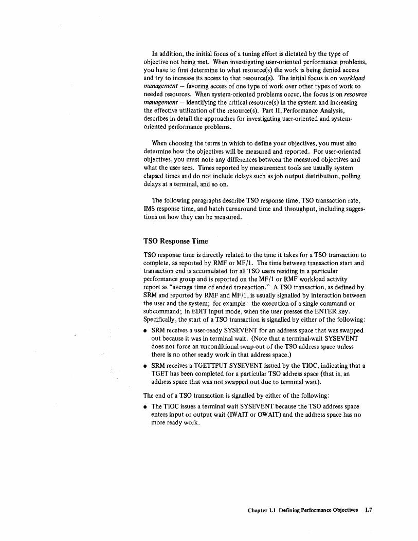
In addition, the initial focus of a tuning effort is dictated by the type of objective not being met. When investigating user-oriented performance problems, you have to first determine to what resource(s) the work is being denied access and try to increase its access to that resource(s). The initial focus is on workload management - favoring access of one type of work over other types of work to needed resources. When system-oriented problems occur, the focus is on resource management - identifying the critical resource(s) in the system and increasing the effective utilization of the resource(s). Part II, Performance Analysis, describes in detail the approaches for investigating user-oriented and systemoriented performance problems.
When choosing the terms in which to define your objectives, you must also determine how the objectives will be measured and reported. For user-oriented objectives, you must note any differences between the measured objectives and what the user sees. Times reported by measurement tools are usually system elapsed times and do not include delays such as job output distribution, polling delays at a terminal, and so on.
The following paragraphs describe TSO response time, TSO transaction rate, IMS response time, and batch turnaround time and throughput, including suggestions on how they can be measured.
TSO Response Time
TSO response time is directly related to the time it takes for a TSO transaction to complete, as reported by RMF or MF /1. The time between transaction start and transaction end is accumulated for all TSO users residing in a particular performance group and is reported on the MF /1 or RMF workload activity report as "average time of ended transaction." A TSO transaction, as defined by SRM and reported by RMF and MF /1, is usually Signalled by interaction between the user and the system; for example: the execution of a single command or subcommand; in EDIT input mode, when the user presses the ENTER key. Specifically, the start of a TSO transaction is signalled by either of the following:
• SRM receives a user-ready SYSEVENT for an address space that was swapped out because it was in terminal wait. (Note that a terminal-wait SYSEVENT does not force an unconditional swap-out of the TSO address space unless there is no other ready work in that address space.)
• SRM receives a TGETTPUT SYSEVENT issued by the TIOC, indicating that a TGET has been completed for a particular TSO address space (that is, an address space that was not swapped out due to terminal wait).
The end of a TSO transaction is signalled by either of the following:
• The TIOC issues a terminal wait SYSEVENT because the TSO address space enters input or output wait (IWAIT or OWAIT) and the address space has no more ready work.
Chapter 1.1 Defining Performance Objectives 1.7

• SRM receives anotherTGETTPUT SYSEVENT indicating that a subsequent command has been received. This signals the end of the previous transaction and the beginning of a new transaction.
Note, however, that the response time as measured by RMF or MF/l is an average and can be different from that which individual end users see. In addition, the RMF or MF 11 reported time does not include factors such as line speed, control unit delay, polling delay, or the length of time the teleprocessing access method requires to decode the user i.d. from the input data stream. Some experiments have shown as much as a two-second delay due to such factors.
TSO Transaction Rate
TSO transaction rate is the number of TSO transactions that complete per unit of time. There is a direct relationship between transaction rate and response time, as illustrated in the following formula:
transaction rate ;::: number of active terminals user time + response time
where user time consists of thinking and typing time. As response time decreases, transaction rate increases. It has also been observed that faster response time often indirectly results in less user time, again resulting in an increased transaction rate. Note that if transaction rate, response time, and the number of active terminals are known, this formula can be used to compute user time.
The "ended transactions" field on the RMF or MF 11 workload activity report gives the number of transactions that ended in the interval; the transaction rate can then be computed as the number of ended transactions divided by the interval. Note, however, that, for VT AM, end-of-screen on 3270s is also considered a transaction in the RMF or MF/l counts and, therefore, is reflected in the "ended transactions" field.
IMS Response Time
The transaction response report, produced by the IMSNS statistical analysis utility programs, reports response times by transaction type, including: total number of responses; longest and shortest responses; and average response times achieved by 95%, 75%, 50%, and 25% of the transactions. The time reported is from complete receipt of the input message until the response message to the terminal is successfully dequeued. Input to the IMS/VS statistical analysis utility programs is the IMS log tape. To obtain a transaction response report for certain time periods, execute the IMS/VS log transaction analysis utility program with appropriate start and end times to obtain a log tape for the desired period. For details, see the IMS/VS Utilities Reference Manual.
1.8 OSjVS2 MVS Performance Notebook

Batch Throughput and Turnaround Time
Batch throughput is available from the RMF or MF /1 workload activity report. For batch work, a transaction as reported by RMF or MF /1 is a job, unless different performance group numbers are assigned to the steps of a job; in such cases, each job step is considered a transaction. If performance group numbers are assigned only on a job basis, you can compute batch throughput as "ended transactions" for batch performance groups, divided by the RMF or MF /1 interval.
Using a data reduction program, you can compute turnaround time and throughput from information in SMF record type 5, which contains fields for the time the reader recognized the JOB card and the time the job terminated. Note that the turnaround time computed via SMF does not include delays entering the job into the system and distributing output, which increase turnaround time from the user's point of view.
Step 3: Documenting the Workload
After deciding on and defining the terms in which to measure performance, the next step in writing performance objectives is to understand and document the current workload on the system. This includes the amount and the categories of work:
• priority of the work.
• different periods of time during which objectives and priorities vary for the same work.
• resource requirements of the work.
• the types of users that require different objectives.
• the ability to track and report on work according to the instal1ation's needs -for example, department breakdowns.
Start with the categories of work that were defined under the prior system: batch job classes, IMS transaction types, and so on. Usually, however, these categories were not fully defined. Figure 1.2 suggests data to collect to fully define each category of work. (Note that figure 1.2 includes resource requirements for each category of work. When initially defining the categories, the resource requirements will probably reflect expected resource usage; measuring actual resource usage on MVS is described in more detail in step 5.)
Once the categories are defined, review them for apparent errors. The purpose of the different categories is to distinguish work according to different resource requirements, different objectives that must be met, different priorities, and so on. For example, all jobs submitted from similar development groups in different locations are expected to receive the same turnaround time. However, because of distribution of the completed work to different locations, and possible time differences in actually returning output to the submitters, you might want to further separate this work - to give priority to jobs that have to be distributed to locations in different time zones, where delays in turnaround time can have a more significant effect on the users.
Chapter 1.1 Defining Performance Objectives 1.9
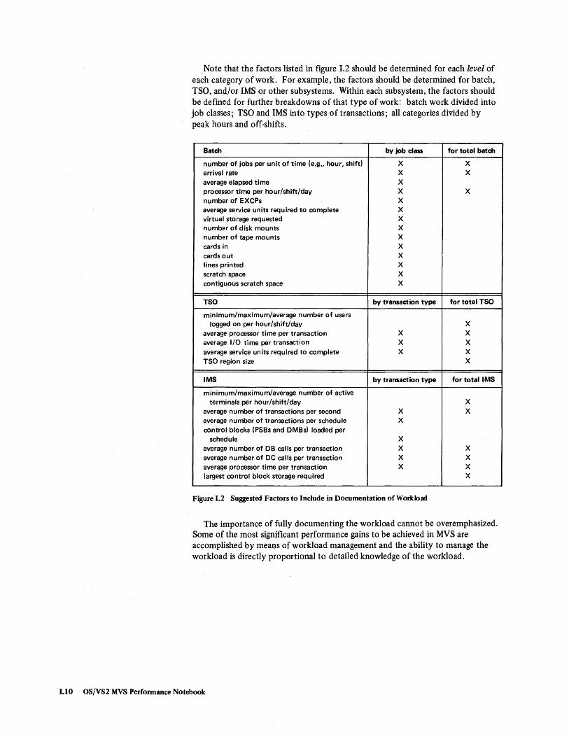
Note that the factors listed in figure 1.2 should be determined for each level of each category of work. For example, the factors should be determined for batch, TSO, and/or IMS or other subsystems. Within each subsystem, the factors should be defined for further breakdowns of that type of work: batch work divided into job classes; TSO and IMS in to types 0 f transactions; all categories divided by peak hours and off-shifts.
Batch by job class for total batch
number of jobs per unit of time (e.g., hour, shift) X X arrival rate X X average elapsed time X processor time per hour/shift/day X X number of EXCPs X average service units required to complete X virtual storage requested X number of disk mounts X number of tape mounts X cards in X cards out X lines printed X scratch space X contiguous scratch space X
TSO by transaction type for total TSO
minimum/maximum/average number of users logged on per hour/shift/day X
average processor time per transaction X X average I/O time per transaction X X average service units required to complete X X TSO region size X
IMS by transaction type for total IMS
minimum/maximum/average number of active terminals per hour/shift/day X
average number of transactions per second X X average number of transactions per schedule X control blocks (PSBs and DMBs) loaded per
schedule X average number of DB calls per transaction X X average number of DC calls per transaction X X average processor time per transaction X X largest control block storage required X
Figure 1.2 Suggested Factors to Include in Documentation of Workload
The importance of fully documenting the workload cannot be overemphasized. Some of the most significant performance gains to be achieved in MVS are accomplished by means of workload management and the ability to manage the workload is directly proportional to detailed knowledge of the workload.
1.10 OS!VS2 MVS Performance Notebook

Step 4: Setting the Objectives
Once the workload is categorized, set objectives for each category of work. Experience with some MVS systems shows that installations don't always know the specific response and turnaround requirements of different users. As a starting point, use the response or turnaround time achieved on the pre-MVS system. If such data was not formally reported, it is still probably available from old trace tapes, the output of old reduction programs, the operator log, or similar sources. Examine the objectives achieved on the pre-MVS system in light of user requirements and the priority of the work. If necessary, revise the objectives met on the pre-MVS system.
Many installations state objectives for a percentage of the transactions in a class - for example, 90% of TSO transactions should receive a three-second response time; 85% of the jobs in class A should receive turnaround time of one hour. If you state objectives in these terms, also set an objective for the "leftover" percentage of transactions - in the preceding example, for the 10% of TSO transactions and the 15% of jobs in class A. For very heavy transactions or jobs, you might want to specify the objectives in terms of service units or processor time received per second. Ensure that objectives are set for 100% of the work in your system.
In setting user-oriented objectives, be sure you take into account any time the user sees that is not reflected in the measurement of the objective. For example, if TSO trivial transactions require a four-second response time, you might set the objective to three seconds to account for polling delays not reflected in RMF or MF /1 measurements of response time.
Step 5: Measuring Resource Requirements
Once MVS is generated and stable, measure the resources actually being used by the different categories of work. To do this, you must choose the means by which you will measure resource consumption (for example, service units, seconds, number of events such as the number of EXCPs, and so on) and the tools by which the resources will be measured. Essentially, you want to identify the amounts of processor, real storage, and I/O resources required for each category of work. Figure I.2 includes resource requirements that might be measured.
By assigning each distinct category of work to a separate performance group, you can obtain data on the processor, real storage, and I/O service units consumed by each category from the RMF workload activity report. Note, however, that there are two exceptions: (1) I/O service for IMS will not be reported, since all IMS EXCPs are issued in key 7; and (2) service will not be reported for privileged address spaces - that is, those address spaces for which you turned on the privileged bit in the PPT to make the address space nonswappable unless it enters long wait. Instead of using the privileged bit, place the address spaces in a domain where the minimum MPL is greater than or equal to the number of address spaces in the domain. The address spaces will not be swapped and RMF will report the service units they use.
Chapter 1.1 Defining Performance Objectives 1.11
If you are using the same batch job classes iri MYS as were used in MYT or SVS, you might want to assign each class to a unique performance group with identical IPS performance objectives; this will help you observe how the job classes are serviced in MVS and might help you identify changes to the job class structure.
Track the resource measurements for an extended period of time so that they encompass all variations in the workload. Job- and transaction-related data should be tracked both as an average and as a distribution, so that you identify exceptional conditions. Such exceptions will help you judge the effectiveness of your workload categories and the possible need for installation controls on the exceptional work. For example:
• Batch jobs whose resource consumption places them in the top ten percent of their class in terms of resource usage might require reclassification.
• If the resource data varies widely for a particular job class - that is, there is no distinct pattern - that job class might require redefinition or a tolerant performance objective.
The resource data collected will further define the categories of work; from this data, you can set resource limits for each category ~ for example, one processor minute for each job in job class X. Once the resource limits for each class are understood, consider installation controls and procedures to track and enforce these limits. Some resource limits, such as elapsed time and resource allocation, can be enforced using SMF exits. Others, such as number of EXCPs or amount of real storage, cannot be enforced while the program is running. You might want to produce exception reports that list jobs/transactions that exceed anyone of the resource limits. Or adjust billing rates for jobs that exceed the resource limits for their class, to provide an incentive to the user to correctly classify his work.
Understanding the resources required for each category of work, at each level, will help you to judge the reasonableness of your objectives and to set capacity limits for each category: the throughput measure which, if exceeded, will impact other work in the system. The following formulas might be useful in helping you determine capacity limits for batch and TSO work:
TSO processor % = average processor seconds per TSO transaction x
transaction rate x 100
b t hat 100 x average processor seconds per job x number of jobs
a c processor 10 = ... . seconds m the measured mterval
Figure 1.3 illustrates a complete performance objective for a batch job class, including the definition of the category, resource requirements, and capacity limits.
1.12 .oS/VS2 MVS Performance Notebook

Batch class = B
Prime shift: 8:00 - 6:00
Class description: short duration batch
Objectives for class:
class turnaround 90% of the jobs will clear the printer in less than 30 minutes (from first card read)
throughput limit - 400 jobs
class resource consumption limits
processor minutes
EXCPs
elapsed time (minutes)
storage requested
disk mounts
tape mounts
cards in
cards out
lines printed
scratch spa ce
contiguous scratch space
for each job in the class
1.00
1000
10
512K
none
none
1000
500
4500
25 cyl
5 cyl
Figure 1.3 Sample Performance Objective for Batch Job Class
Chapter 1.1 Defining Performance Objectives 1.13

1.14 OS/VS2 MVS Performance Notebook

Chapter 1.2 Selecting Measurement Tools
The goal of any performance evaluation is to make the most effective use of the basic system resources: processor, storage, channels, I/O devices, and control units. In order to do this, it is necessary to first determine the specific performance problems that might exist in the system by examining the current use of the resources. Once potential solutions are identified and implemented, it is necessary to re-evaluate resource utilization to judge the effectiveness of the solutions. Measurement tools are the means to determine how resources are being used; any performance analysis effort is, in fact, limited by the software and hardware measurement tools that are available to the installation.
The purpose of this chapter is to present an overview of tools available from IBM and additional techniques that can be used to gather data and measure resource usage in the system. This chapter is divided into the following topics:
• "MVS Measurement Tools," which describes the types of data provided by various tools.
• "Other Sources of MVS Data," including control blocks, the trace table, and SYSl.LOGREC.
• "Writing Data Reduction Programs," which focuses on extracting performancerelated information from SMF and GTF. (Writing data reductions programs to extract information from control blocks and the trace table is described in "Other Sources of MVS Data.")
• "Monitoring Performance," which describes the kind of data you should monitor on a continuous basis, so that you can recognize potential performance problems before they become crises.
MVS Measurement Tools
While SMF, GTF, and MF/l (or RMF) are important IBM measurement tools that exist as part of the MVS system (or as a program product), the installation will usually need additional tools to collect and process all of the data required for a performance evaluation. A number of programs have been written to provide details both system-wide and by address space on system operations such as paging, real storage utilization, and processor utilization. These are the currently available Installed User Programs (lUPs) and Field Developed Programs (FDPs). Most of these programs are data reduction tools for SMF or GTF. Others are software monitors, which use their own monitoring facilities to extract data and their own reduction capabilities to format the data. Many of these tools can and should be used together (either concurrently or sequentially) to get the most realistic and comprehensive picture of system resources as possible.
Chapter 1.2 Selecting Measurement Tools 1.15
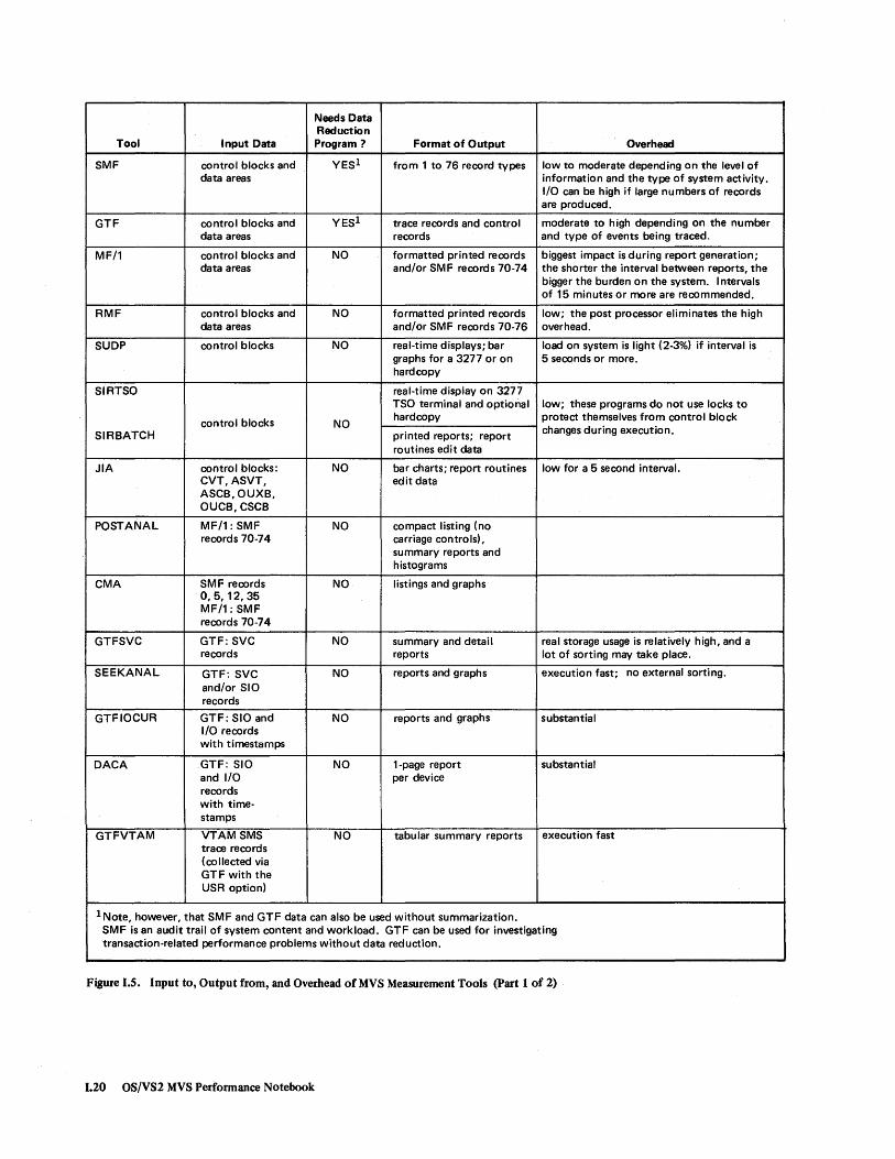
The following figures provide a comparison of various measurement tools available from IBM and of hardware monitors. (Note: IBM does not market hardware monitors. Any statement about their capabilities is based upon IBM's general knowledge of hardware monitors. While the statements are believed to be true, customers using hardware monitors should rely on their vendors for information. )
• Figure 1.4 gives a general description of each tool.
• Figure 1.5 lists input to and output from the tools.
• Figure 1.6 notes operating characteristics and limitations of the tools.
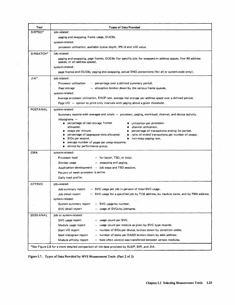
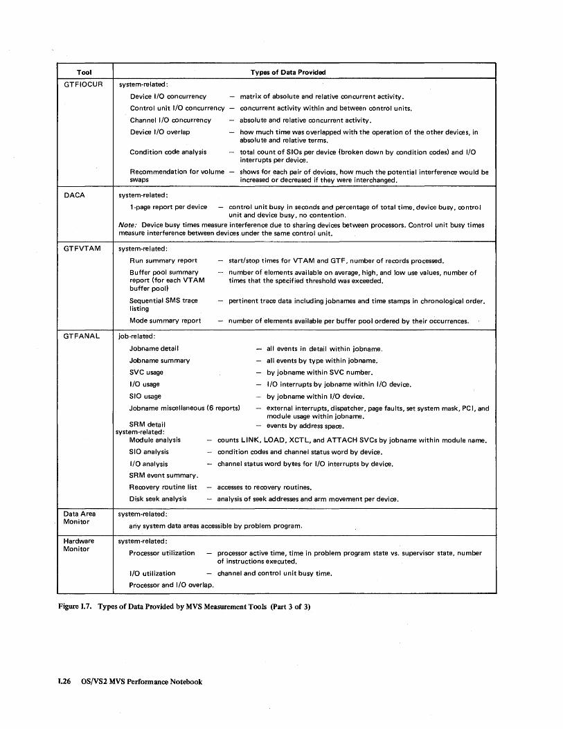
• Figure 1.7 summarizes the types of data provided by the tools.
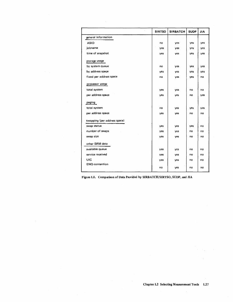
(Note: IMS and JES3 tools are included only in figure 1.4.) In addition, figure 1.8 compares the types of data provided by three software monitor programs: SUDP, SIRTSO/SIRBATCH, and JIA. Figure 1.9 lists the major system resources, the types of data that should be examined for each resource, and the key tools and/or control blocks that can be used to collect the data. (More information on control blocks is included in the next topic, "Other Sources of MVS Data.")
1.16 OS/VS2 MVS Performance Notebook

Tool Type General Description Documentat ion
System Management MVS component collects a large amount of data, a subset of which OS/VS2 SPL: System Facilities (SMF) is performance-related. Emphasis is on job-related Management Facilities,
data. GC28-0706
Generalized Trace MVS component collects a large amount of data; traces system OS/VS2 SPL: Service Facility (GTF) events. Aids, GC28-0674
System Activity MVS component collects system-wide information of a general OS/VS2 SPL: Initializa-Measurement Facility nature; most is performance-related. Evaluates tion & Tuning Guide, (MF/1) hardware performance. GC28-0681
Resource program product same as MF/1 with mOre system data, two OS/VS2 MVS Resource Measurement Facility additional reports, and an offline post processor. Measurement Facility, (RMF) GIM, GC28-0736
MVS Storage Utilization software monitor provides information on the use of real storage SB21-1753 and Display (SUDP) (FDP # 5798-CGT) by particular jobs. LB21-1754
System Information software monitor SIRTSO - runs as a TSO command; provides SH20-1813 Routines (SIR) (lUP #5796-PGB) enough job-related data to give a full picture of
SRM and paging activity. SIRBATCH - runs as a batch job or started task;
collects system and address space data at fixed intervals. Provides more details than SIRTSO.
SVS/MVS System and Job software monitor provides averages of various system activities on SH20-1720 and Impact Analyzer (JIA) (lUP #5796-AJF) an address space basis. LY20-2217
MF/1 Post Analyzer SMF analysis program provides general system-related data via two SB21-1814 and (POSTANAL) (FDP #5798-CHX) report programs: MF1 DFERD (Assembler LB21-1815
Language) and MF1ANLZR (PL/1L More useful for capacity planning than for tuning.
OS/VS Capacity SMF analysis program provides an overview of the usage of various SB21-1835 and Management Aid (CMA) (FOP # 5798-CJB) system functions via two Assembler and five LB21-1836
FORTRAN programs. Useful for capacity planning.
GTF Supervisor Services GT F analysis provides details about SVC usage on a system and SH20-1816 Analyzer (GTFSVC) program job basis. Should be considered one of the major
(I UP # 5796-PG E) tuning tools in situations where supervisor time is critical.
MVS Seek Analysis GTF analysis provides details about SVC and module usage and SH20-1814 Program (SEEKANAL) program about seek operations on OASO on a system or
( I UP # 5796-P JC) job basis. Should be considered one of the major tuning tools.
GTF I/O Concurrency GTF analysis provides details about potential device contention SH20-1815 and (GTFIOCUR) program resulting from concurrent operations on channels LY20-2240
(lUP #5796-PGO) and control units; used to minimize OASO I/O interference.
GTF Direct Access GT F analysis provides details about the interference due to SB21-1654 Contention Analyzer program accessing shared DASD and interference between (DACA) (FDP #5798-CEZ) devices under the same control unit.
GTF VT AM Buffer Trace GTF analysis provides information about the utilization of SH20-1817 Analysis (GTFVTAM) program VT AM buffer pools to aid in designing the right
(lUP #5796-PGF) size pool.
GTF Data Analysis GT·~ analysis handles all types of GTF records; reports seek SB21-1808 Program (GTFANAL) program statistics and statistics about arm movement.
(FDP #5798-CHT)
Generalized Data Area (FDP # 5798-CKK) monitors and displays user or system data areas SB21-1910 and Monitor and Display in OS/VS system; data areas to be monitored LB21-1911 Program (Data Area are indicated by means of control cards. Monitor)
Figure 1.4. General Information on MV8 Measurement Tools (part 1 of 3)
Chapter 1.2 Selecting Measurement Tools 1.17

Tool Type General Description Documentation
Hardware Monitors hardware monitor captures and records electrical signals created by the system during normal operation.
JES3 Monitoring software monitor monitors activity within the JES3 address space on SH20-1881 Facility (JMF) (lUP #5796-PHR) an MVS global processor and records data on the
following: JES3 processor/address space activity; JES3 FCT activity; JES3 spool data management; JES3 device scheduling activity; and JES3 job throughput.
I MS/VS Log Transaction IMS component based on information from the IMS log tape IMS/VS Utilities Analysis Utility Program about individual occurrences of IMS/VS trans- Reference Manual, (OFSILTAO) actions, calculates total response time, time on SH20-9029
the input queue, processing time, and time on the output queue. Produces a new IMS/VS log tape, if specified; a report on disk that can be sorted to produce a sequenced report; a detailed report of transactions in input sequence, if specified; and a summary report.
IMS/VS Statistical IMS component Using the IMS log as input, produces a list of I MS/VS Utilities Analysis Utility Programs messages in line and terminal sequence, a list Reference Manual,
of messages in transaction code sequence, or SH20-9029 statistical reports. Reports include the following: messages queued but not sent; program-to-program messages; line and terminal report, which shows line and terminal loading by time of day; transaction report, which shows loading by transaction code and by time of day; trans-action response report; application accounting report, which includes TCe processor time and counts of all OUI requests; and IMS/VS accounting report, which shows start and stop time for the control region.
IMS/VS Program Isolation IMS component Lists all transactions that had to wait while trying IMS/VS Utilities Trace Report Utility to enqueue on a data base record; prints the Reference Manual, Program (OFSPIRPO) waiting transaction, the holding transaction, and, SH20-9029
if the /TRACE ALL option is used, the elapsed time of the wait.
IMS DC Monitor IMS component provides key values such as elapsed time, IWA IT IMS/VS Utilities time, elapsed processor time, scheduled time to Reference Manual, first OUI call, elapsed execution time, and queue SH20-9029 statistics. The IMS/VS Monitor Report Print Program (0 FSUTR20) summarizes and categorizes the information at various levels of detail, pro-ducing the following reports: system configuration; statistics from buffer pools; region summary; region IWAIT; programs by region; program summary; program I/O; communication summary; communication IWAIT; transaction queueing; OL/I call summary; and distribution appendix.
Figure 1.4. General Infonnation on MVS Measurement Tools (Part 2 of 3)
1.18 OS/VS2 MVS Performance Notebook

Tool Type General Description Documentat ion
IMS Monitor Summary (FOP #5798-COT) a set of programs designed to process OFSTRAPC SB21-1582 and System Analysis output from I MS/VS Monitor (I MS/VS 1.0.1). Program (I MSASAP) It uses a subset of the data collected by
o FSTRAPC to produce several selectable additional reports designed to fill the needs of management, system analysts, and programmers.
IMS Log Tape Analysis (FOP #5798-CAQ) provides information on response times and SB21-1402 message traffic.
IMS/VS Virtual Storage GTF reduction provides an IMS/VS memory map, showing the SB21-2003 Analysis program name, real storage locations, and length of various
(FOP #5798-CNC) pools and modules in the IMS/VS system, and three page fault activity reports designed to trace, summarize, and categorize page faults associated with the I MS/VS system.
IMSMAP/VS Data Base (IUP #5796-PCY) provides two data base mapping programs: SH20-1539 Mapping Programs OBOMAP, which builds and prints maps of IMS
physical and logical data bases and a descriptive report of each data base; and PSBMAP, wh ich builds and prints maps of IMS physical and logical data bases associated with program specification blocks. Note: IMSMAP ((UP #57960-PBC) is a prerequisite to the installation of IMSMAP/VS.
Figure 1.4. General Information on MVS Measurement Tools (Part 3 of 3)
Chapter 1.2 Selecting Measurement Tools 1.19
Needs Data Reduction
Tool Input Data Program? Format of Output Overhead
SMF control blocks and YESl from 1 to 76 record types low to moderate depending on the level of data areas information and the type of system activity.
I/O can be high if large numbers of records are produced.
GTF control blocks and YESl trace records and control moderate to high depending on the number data areas records and type of events being traced.
MF/1 control blocks and NO formatted printed records biggest impact is during report generation; data areas and/or SMF records 70·74 the shorter the interval between reports, the
bigger the burden on the system. Intervals of 15 minutes or more are recommended.
RMF control blocks and NO formatted printed records low; the post processor eliminates the high data areas and/or SMF records 70·76 overhead.
SUDP control blocks NO real·time displays; bar load on system is light (2·3%) if interval is graphs for a 3277 or on 5 seconds or more. hardcopy
SIRTSO real·time display on 3277 TSO terminal and optional low; these programs do not use locks to
control blocks NO hardcopy protect themselves from control block
SIRBATCH printed reports; report changes during execution.
routines edit data
JIA control blocks: NO bar charts; report routines low for a 5 second interval. CVT,ASVT, edit data ASCB,OUXB, OUCB, CSCB
POSTANAL MF/1: SMF NO compact listing (no records 70-74 carriage controls),
summary reports and histograms
CMA SMF records NO listings and graphs 0,5,12,35 MF/1: SMF records 70-74
GTFSVC GTF: SVC NO summary and detail real storage usage is relatively high, and a records reports lot of sorting may take place.
SEEKANAL GTF: SVC NO reports and graphs execution fast; no external sorting. and/or SIO records
GTFIOCUR GTF: SIO and NO reports and graphs substantial I/O records with timestamps
DACA GTF: SIO NO 1-page report substantial and I/O per device records with time-stamps
GTFVTAM VTAM SMS NO tabular summary reports execution fast trace records (collected via GTF with the USR option)
1 Note, however, that SMF and GTF data can also be used without summarization. SMF is an audit trail of system content and workload. GTF can be used for investigating transaction-related performance problems without data reduction.
Figure 1.5. Input to, Output from, and Overhead of MVS Measurement Tools (part 1 of 2)
1.20 OS/VS2 MVS Performance Notebook

Needs Data Reduction
Tool Input Data Program? Format of Output Overhead
GTFANAL GTF: DSP, NO broad range of reports number of output pages is high EXT, PCI, available from single run SRM, SIO, I/O, SVC, and RR records
Data Area Monitor data areas NO detail report, each line of low selected by which consists of a user-installation specified description and
as many observations as will fit on the print line; and summary report, which displays the summary data for each of the user-defined variables.
Hardware NO real-time measurements; low; they might not interrupt processing Monitors data is summarized and if ruri independently of system processor
written to tape; programs time. format it into graphs.
Figure r.S. Input to, Output from, and Overhead of MVS Measurement Tools (Part 2 of2)
Chapter 1.2 Selecting Measurement Tools 1.21

Tool Operating Characteristics Limitations Notes
SMF • parameters specify record types and No data collected for system tasks or • should be used with MF/l or exit routines. problem programs started from console RMF.
• SMF buffer size should be in 4K- or running in system keys. Data can be • should be used to locate 8K range in order to prevent collected for a subsystem only if it
dominant jobs, programs, excessive I/O and ENQ delays. is started as a job in the form of a card
and files. deck or invoked through an internal
• use IE FU83 exit routine to avoid reader procedure. writing unnecessary records, but retain the capability to periodi-cally sample all work in terms of storage, EXCPs, blocksizes, etc.
• turn off unused exits.
GTF • options specify the system events Does not provide environmental data In response or turnaround situ-to be traced. such as storage size, alternate paths, ations, time stamping should be
run at a high dispatching priority and volume serial numbers. Issue the used. • DISPLAY UNITS command to obtain to reduce lost events since it is generally used for short spurts of the device address and the volume
system activity . currently mounted on the device.
MF/1 and RMF • options specify the reports and • only one can be active at a time; • can be used with SMF to intervals to be generated. must be stopped and restarted obtain a complete picture
• run in RECORD mode to collect to change options. of system workload (see
data in machine readable form and • does not recognize the type of SPL: Initialization and
have it written to the active SMF work being run on the system; Tuning Guide). Use these
data set. however, you can obtain data on two tools to compare paging rates, I/O activity, and services
• to trace individual jobs, assign each distinct categories of work by of a problem program and the
to its own performance group. assigning different types of work to system.
different performance groups.
• put each IMS MPR in a different • does not report services of • RMF has a post processor performance group to get the privileged address spaces; instead to read in RMF SMF records processor utilization, absorption of using the privileged bit in the and pri nt reports. rate, and task time for each one. PPT, assign "privileged" address
spaces to a domain where the minimum MPL is greater than or equal to the number of address spaces in the domain to ensure they are not swapped.
SUDP • must run non-swappable and Does not run under TSO. authorized.
• monitor interval and display types can be changed by a light pen.
SIRTSO • subcommands specify the address spaces to gather information for: batch, TSO-users, swapped-in, or all.
• re-entrant program; can be placed Used primarily to supplement
in SYS1.LPALIB. data provided by MF/1 or RMF with detailed information about
• uses TPUT full-screen facility; specific address spaces. specify FULLSCR=YES in the TCAM MCP.
SIRBATCH Must reside in an authorized library.
Figure 1.6. Operational Considerations for MVS Measurement Tools (part 1 of 2)
1.22 OS/VS2 MVS Performance Notebook
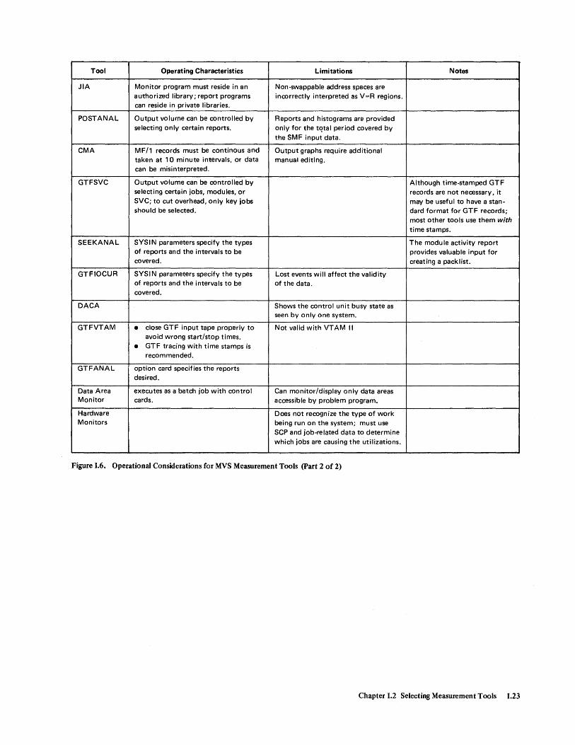
Tool Operating Characteristics Limitations Notes
JIA Monitor program must reside in an Non-swappable address spaces are authorized library; report programs inrorrectly interpreted as V=R regions. can reside in private libraries.
POSTANAL Output volume can be rontrolled by Reports and histograms are provided selecting only certain reports. only for the tqtal period rovered by
the SMF input data.
CMA MF/1 records must be continous and Output graphs require additional taken at 10 minute intervals. or data manual editing. can be misinterpreted.
GTFSVC Output volume can be rontrolled by Although time-stamped GTF selecting certain jobs, modules, or records are not necessary, it SVC; to cut overhead, only key jobs may be useful to have a stan-should be selected. dard format for GTF records;
most other tools use them with time stamps.
SEEKANAL SYSIN parameters specify the types The modu Ie activity report of reports and the intervals to be provides valuable input for covered. creating a pack list.
GTFIOCUR SYSIN parameters specify the types Lost events will affect the validity of reports and the intervals to be of the data. covered.
DACA Shows the control unit busy state as seen by only one system.
GTFVTAM • close GTF input tape properly to Not valid with VTAM II avoid wrong start/stop times.
• GTF tracing with time stamps is recommended.
GTFANAL option card specifies the reports desired.
Data Area executes as a batch job with rontrol Can monitor/display only data areas Monitor cards. accessible by problem program.
Hardware Does not recognize the type of work Monitors being run on the system; must use
SCP and job-related data to determine which jobs are causing the utilizations.
Figure 1.6. Operational Considerations for MVS Measurement Tools (part 2 of 2)
Chapter 1.2 Selecting Measurement Tools 1.23

Tool
SMF
GTF
MF/1
RMF
SUDP*
Types of Data Provided
job-re lated:
Type 4/34 records - swap counts, page-in/page-out counts, EXCP counts (including VIO accesses), processor time and storage used for a step.
Type 5/35 records - Processor time under TCSs and SRSs, and job service unit count.
Type 14/15 records - EXCP counts and other information for data sets.
Type 26 record - actual SYSIN/SYSOUT line and card count.
system-related (collected during MF/1 or RMF interval): \
Type 70-76 records - processor, paging, workload, channel, device, page-swap data set, and trace activity.
system-re lated:
SID trace records - shows seek activity on a device and SID operations.
SVC trace records - identifies type, quantity, and users of supervisor services, such as ENQ/DEQ activity (including the resource namel.
SRM trace records - SRM activity and SYSEVENTS.
I/O trace records - shows I/O interrupts by device.
DSP trace records - shows all units of work dispatched by the system.
PI trace records - program interrupts.
EXT trace records - external interrupts (clock and signal processor interrupts).
system-related (collected during each interval):
CPU Activity Report - processor wait time. Processor utilization = 100% - wait percentage.
Channel Activity Report - number of successful SIOs issued to each channel, percent of time channel busy, percent busy while processor waited.
I/O Device Activity Report - number of successful SIOs issued to each device, percent of time device busy, average number of requests enqueued on each device.
Paging Activity Report - details about paging demands, a snapshot of real and auxiliary page storage, and swapping statistics.
Workload Activity Report - information on workload activity for each performance group period and for the system as a whole.
Same as MF/1, plus the following:
additional data in the Paging Activity Report
additional data in the Workload Activity Report
Page/Swap Data Set Activity Report
ASM/RSM/SRM Trace Activity Report
job-related:
- SRM swap out counts, sampled minimum, maximum, and average real and auxiliary page storage.
- 10C, CPU, and MSO service swaps by performance group and domain numbers.
- statistics on individual data set usage.
- sampled values of fields from PVT and ASMVT control blocks, SRM Data Area, and SRM Domain Tables.
Real Storage utilization
system-related:
- percent used/fixed by each job, TSO user, and system task, and a swap indication.
Paging Rates - demand paging, VIO paging, and swapping.
Internal Queues of Frames - available pages, common, SQA, LSQA, and local frames and their status.
*See Figure 18 for a more detailed comparison of the data provided by SUDP, SIR, and JIA.
Figure 1.7. Types of Data Provided by MVS Measurement Tools (part 1 of 3)
1.24 OS!VS2 MVS Performance Notebook
Tool
SIRTSO*
SIRBATCH*
JIA*
POSTANAL
CMA
GTFSVC
SEEKANAL
Types of Data Provided
job-related:
paging and swapping, frame usage, OUCBs.
system-re lated:
processor utilization, available queue depth, IPS id and UIC value.
job-related:
paging and swapping, page frames, OUCBs (for specific job, for swapped-in address spaces, first 40 address spaces, or all address spaces).
syste more lated:
page frames and OUCBs, paging and swapping, actual ENQ contentions (for all or system-wide only).
job-related:
Processor utilization
Real storage
system-re lated:
- percentage over a defined summary period.
- allocation broken down by the various frame queues.
Average processor utilization, EXCP rate, average real storage per address space over a defined period.
Page I/O - option to print only intervals with paging above a given threshold.
system-related:
Summary reports with averages and totals - processor, paging, workload, channel, and device activity.
Histograms -• percentage of real storage frames • utilization per processor.
allocated. • channel utilization. • swaps per minute. • percentage of transactions ending 1st period. • percentage of pagespace slots allocated. • ratio of ended transactions per number of swaps. • SIOs per second. • non-swap paging rate. • average number of pages per swap sequence. • service by performance group.
system-related:
Processor load - for batch, TSO, or total.
Storage usage - swapping and paging.
Application development - job steps and TSO sessions.
Percent of week processor is active.
Daily load profile.
job-related:
Job summary report
Job detail report
system-related:
- SVC usage per job in percent of total SVC usage.
- SVC usage for a specified job by TCB address, by module name, and by PSW address.
System summary report - SVC usage by number.
SVC detail report - usage of SVCs by jobname.
job or system-related:
SVC usage report
Module usage report
Start I/O report
Seek histogram report
Module affinity report
- usage count per SVC.
- usage count per module as given by SVC type records.
- number of SIOs per device, broken down by condition codes.
- number of seeks per DASD broken down by seek address.
- how often control was transferred between certain modules.
*See Figure 1.8 for a more detailed comparison of the data provided by SUDP, SIR, and JIA.
Figure 1.7. Types of Data Provided by MVS Measurement Tools (Part 2 of 3)
Chapter 1.2 Selecting Measurement Tools 1.25
Tool
GTFIOCUR
DACA
GTFVTAM
GTFANAL
Data Area Monitor
Hardware Monitor
Types of Data Provided
system-related:
Device I/O concurrency - matrix of absolute and relative concurrent activity.
Control unit I/O concurrency - concurrent activity within and between control units.
Channel I/O concurrency - absolute and relative concurrent activity.
Device I/O overlap
Condition code analysis
- how much time was overlapped with the operation of the other devices, in absolute and relative terms.
- total count of SIOs per device (broken down by condition codes) and I/O interrupts per device.
Recommendation for volume swaps
- shows for each pair of devices, how much the potential interference would be increased or decreased if they were interchanged.
system-related:
1-page report per device - control unit busy in seconds and percentage of total time, device busy, control unit and device busy, no contention.
Note: Device busy times measure interference due to sharing devices between processors. Control unit busy times measure interference between devices under the same control unit.
system-re I ated :
Run summary report
Buffer pool summary report (for each VT AM buffer pool)
Sequential SMS trace listing
Mode summary report
job-related:
Jobname detail
Jobname summary
SVC usage
I/O usage
SIO usage
- start/stop times for VT AM and GTF, number of records processed.
- number of elements available on average, high, and low use values, number of times that the specified threshold was exceeded.
- pertinent trace data including jobnames and time stamps in chronological order.
- number of elements available per buffer pool ordered by their occurrences.
- all events in detail within jobname.
- all events by type within jobname.
- by jobname within SVC number.
- I/O interrupts by jobname within I/O device.
- by job name within I/O device.
Jobname miscellaneous (6 reports) - external interrupts, dispatcher, page faults, set system mask, PCI, and
SRM detail system-related:
Module analysis
SIO analysis
I/O analysis
SRM event summary.
module usage within jobname. - events by address space.
- counts LINK, LOAD, XCTL, and ATTACH SVCs by jobname within module name.
- condition codes and channel status word by device.
- channel status word bytes for I/O interrupts by device.
Recovery routine list - accesses to recovery routines.
Di.sk seek analysis - analysis of seek addresses and arm movement per device.
system-related:
any system data areas accessible by problem program.
system-related:
Processor utilization - processor active time, time in problem program state vs. supervisor state, number of instructions executed.
I/O utilization - channel and control unit busy time.
Processor and I/O overlap.
Figure 1.7. Types of Data Provided by MVS Measurement Tools (part 3 of 3)
1.26 OS/VS2 MVS Performance Notebook
SIRTSO SIRBATCH SUDP JIA
general information
ASID no yes yes yes
jobname yes yes yes yes
time of snapshot yes yes yes yes
storage usage
by system queue no yes yes yes
by address space yes yes yes yes
fixed per address space no yes yes no
processor usage
total system yes yes no no
per address space yes yes no yes
~ total system no yes yes yes
per address space yes yes no no
swapping (per address space)
swap status yes yes yes no
number of swaps yes yes no no
swap size yes yes no no
other SRM data
available queue yes yes no no
service received yes yes no no
UIC yes yes no no
ENQ contention no yes no no
Figure I.S. Comparison of Data Provided by SIRBATCH/SIRTSO, SUDP, and JIA
Chapter 1.2 Selecting Measurement Tools 1.27

Data Collected for System Resource Tools to Use Control Blocks to Use
I. Processor Time
for total system MF/1 or RMF CCT (processor SMF record 70 management control SIR table) JIA RMCT POSTANAL CMA Hardware Monitor
for supervisor activities GTF SVC record SEEKANAL
for individual jobs SMF records 4/34 (for step) ASCB SMF records 5/35 (for job) SIRBATCH JIA
for installation-defined groups RMF of work (CPU service)
II. Storage Usage
for total system (real) RMF PVT SIRBATCH PFT JIA CMA
for individual jobs (real) SUDP ASCB SIRBATCH JIA
for installation-defined groups RMF of work (MSO service)
for IMS IMS/VS Virtual Storage Analysis
individual job/job step working SIRBATCH SPCT set size OUCB
for job steps (virtual) SMF records 4/34
nucleus (real) RMF PVT SUDP
SQA (real) SUDP PFT SIRBATCH
LPA and CSA (real) SUDP PFT SIRBATCH
common area (virtual) RMF PVT SUDP
common area paging MF/1 or RMF PVT SMF record 71 SIRBATCH
total system paging MF/1 or RMF PVT SM F record 71 RMCT SUDP SIR JIA POSTANAL
Figure 1.9. Sources of Data on System Resources (part 1 of 2)
1.28 OS/VS2 MVS Performance Notebook

Data Collected for System Resource Tools to Use Control Blocks to Use
II. Storage Usage - (continued)
IMS paging IMS!VS Virtual Storage Analysis
job step swap size RMF PVT SMF records 4/34: OUCB
pages swapped
total number swaps
individual job swapping SIR
job workload level SIRTSO OUCB
III. I/O Activity
channels MF/1 or RMF RMCT SMF record 73 GTF 510-1/0 records POSTANAL GTFIOCUR Hardware Monitor
devices MF/1 or RMF SMF record 74 GTF 510-1/0 records POSTANAL SEEKANAL GTFIOCUR DACA GTFANAL
control units GTF 510-1/0 records GTFIOCUR DACA Hardware Monitor
volume - tape MF/1 or RMF SMF records 19/21
volume - DASD SMF records 14/15 MF/1 or RMF GTF 510 record SYS1.LOGREC
EXCPs for job SMF records 4/34,14/15, 40,64
for installation-defined groups RMF of work (IOC service)
EXCPs for system JIA GTFSVC
Figure 1.9. Sources of Data on System Resources (Part 2 of 2)
Chapter 1.2 Selecting Measurement Tools 1.29

Other Sources of MVS Data
Be aware that the measurement tools described in the previous section do not necessarily provide a complete evaluation of the current performance of a system. They can not totally determine how and under what conditions each resource is being used, nor can they provide information about the existing system configuration while the data is being collected. It is therefore important to use a number of techniques to get information about the system. Additional sources of information on the system environment and activities in the system include the following:
• SYSGEN stage I listing
• JESGEN listing
• P ARMLIB listing
• procedure library listings
• VTOC listings of on-line volumes
• output of the DISPLAY M command for configuration information
• output of the display units command for on-line DASD and their attributes (d u, dasd, online)
• the SYSl.LOGREC data set
• system control blocks
• the system trace table.
This section describes performance-related data that can be derived from control blocks, the trace table, and the SYSl.LOGREC data set.
Control Blocks
System control blocks, available for direct examination while the system is operating, contain descriptive and status information about work executing in the system. Most of the information resides in globally addressable storage and can be monitored on a periodic basis by a user-written data reduction program. A data reduction program can generate information from control blocks such as:
• the identification of users that are swapped into real storage.
• the amount of real storage being occupied.
• how processor time is being apportioned to users; and so on.
In general, this type of information is contained in control blocks that are allocated on an address space basis, although system-wide information of possible interest is also available.
System control blocks are especially useful for determining an address space's use of storage over a particular interval. The ASCB, RSM header, and OUXB contain frame counts on an address-space basis that are dynamically updated; the SPCT also contains frame counts on an address-space basis, but the counts are updated only when an address space is swapped out. The PVT contains systemwide frame counts. By monitoring data on an address space's storage usage, you can observe and analyze activities such as:
• The address space has no allocated frames - it is swapped out.
• The address space has fixed an unusually large number of fra:mes and is tying up storage.
1.30 OS/VS2 MVS Performance Notebook
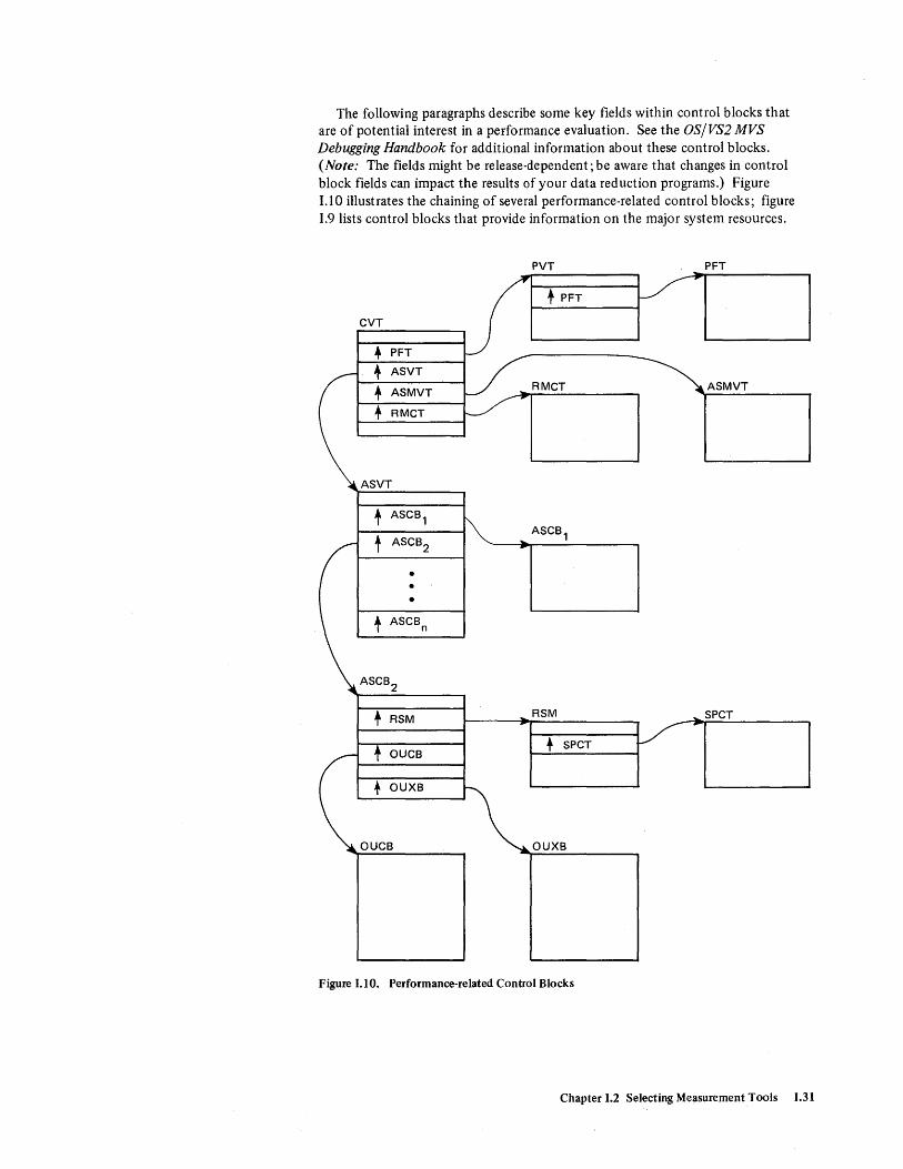
The following paragraphs describe some key fields within control blocks that are of potential interest in a performance evaluation. See the OS/VS2 MVS Debugging Handbook for additional information about these control blocks. (Note: The fields might be release-dependent; be aware that changes in control block fields can impact the results of your data reduction programs.) Figure 1.10 illustrates the chaining of several performance-related control blocks; figure 1.9 lists control blocks that provide information on the major system resources.
PVT PFT
J ~-~
+ PFT
CVT
• PFT
l/:RMCT + ASVT
+ ASMVT ASMVT
~-.. • RMCT
ASVT
t ASCB,
~ ( t ASCB
2
.... ASCB,
• • •
t ASCB n
ASCB2
+ RSM RSM ... SPCT
/ • SPCT + DUCB
• DUXB
DUCB DUXB
Figure I.I0. Performance-related Control Blocks
Chapter 1.2 Selecting Measurement Tools 1.31

Page Vector Table - PVT
The PVT, pointed to by the CVT, contains the following system-wide data that can be of interest to system performance:
PVTAFC Available frame count.
PVTNPIN to These fields contain counters of system paging; the sum of these PVTCAVR fields provide a count of the total system paging.
PVTCFMCT Contains a count of the frames allocated to LP A and CSA.
Page Frame Table - PFT
The PFT, pointed to by the PVT, contains one entry for each real frame in the system, with the exception of the nucleus. Each entry identifies the following:
• the "user" of the frame: the ASID if owned by an address space; X'FFFF' if a system frame; or logical group number, if last used for a VIO page.
• the frame type.
• the fix status.
• the virtual address of the frame.
• the unreferenced interval count (UIC).
SRM Control Table - RMCT
The RMCT is pointed to by the CVT. Following are several fields containing system-wide data of potential interest to performance:
CCVUTILP Contains short-term processor utilization (PCT).
CCVLGUTL Contains long-term processor utilization (PCT * 256).
MCVPTR The non-swap paging rate.
Auxiliary Storage Manager Vector Table - ASMVT
The ASMVT is pointed to from the CVT and contains several system-wide items of potential interest:
ASMSLOTS Contains a count of the number of slots in the paging subsystem.
ASMVSC Contains a count of total slots allocated to VIO.
ASMNVSC Contains a count of total slots allocated for non-VIO slots.
ASMERRS Contains a count of slots unavailable due to I/O errors.
ASMIORQR Contains a count of I/O requests received for processing by ASM.
ASMIORQC Contains a count of I/O requests completed by ASM.
ASMBURST Contains a burst value in microseconds (set to 50000) which is
1.32 OS/VS2 MVS Performance Notebook
used to compute the maximum number of paging requests to place in a single channel program.

Address Space Control Block - ASCB
The ASVT contains an entry for each potential address space. Each entry points to an ASCB, which contains job-related data. The following fields in the ASCB are of interest:
ASCBSEQN
ASCBDP
ASCBEJST
ASCBSWCT
ASCBVSC
ASCBNVSC
ASCBFMCT
ASCBJBNI
ASCBJBNS
ASCBSRBT
The sequence number of this ASCB on the dispatching queue. Valid only if the address space is currently swapped-in.
The current dispatching priority for this address space. Valid only if the address space is swapped-in.
This doubleword (in time-of-day clock format) represents the total task time received by this address space.
Contains a count of the number of short waits issued by this address space. This value is used in the APG mean-time-to-wait calculation.
Contains a count of the total number of VIO slots allocated within the page data sets for this address space.
Contains a count of the total number of non-VIO slots allocated within the page data sets to this address space.
Contains a count of the number of real storage page frames currently occupied by this address space.
Contains a pointer to the 8-character jobname for a batch job. Zero if not a batch job.
Contains a pointer to the 8-character jobname for started tasks, mounts, and TSO users.
This doubleword (in time-of-day clock format) contains the· SRB time accumulated by this address space.
Swap Communication Table - SPCT
The SPCT indicates LSQA and fixed pages that are included in the working set for swapped-out address spaces, and contains other address-space-related swap information.
SRM User Control Block - OUCB
The ASCB for an address space contains a pointer to the OUCB. The OUCB is the key SRM control block for job-related data and contains valuable information about how the SRM sees the address space. The following fields are of primary concern in a performance evaluation:
OUCBQFL This flag byte contains several indicators. OUCBOUT indicates an address space is swapped out but ready to run (on the OUT queue). OUCBOFF indicates the address space is swapped out but not ready to run (on the WAIT queue).
Chapter 1.2 Selecting Measurement Tools 1.33

OUCBEFL This flag byte contains several indicators. OUCBLWT indicates that the address space is in a terminal wait. OUCBQSS/OUCBQSC indicate, respectively, that a quiesce has started and has been completed. (This field can indicate, for example, whether a TSO user is swapped out due to a long wait/terminal wait situation (normal) or due to SRM swapping - that is, if OUCBQSS and OUCBQSC are on with no indication of long wait or terminal wait.)
OUCBSWC Contains a count of the number of swaps that have occurred during the life of the current transaction.
OUCBPSO Contains the number of pages swapped out at the last swap-out of this address space.
OUCBWSS Contains the number of pages swapped in at the last swap-in of this address space. In effect, this is SRM's view of the working set size of this address space; however, it is updated only at swap-out time.
OUCBSRC This one-byte field is of interest in order to determine why the SRM swapped out an address space, as follows:
binary value '01 ' '02' '03' '04' 'OS' '06' '07' '08' '09'
meaning output terminal wait input terminal wait long wait auxiliary storage shortage real pageable storage shortage detected wait requested by the address space enqueue exchange exchange on recommendation value
'OA' unilateral swap-out
OUCBWMR Contains the current normalized workload level for this address space.
OUCBRMR Contains a recommendation value for the current resource use routines.
System Resources Manager User Extension Block - OUXB
The OUXB is also pointed to by the ASCB. It contains data about an address space that is not required by the SRM while that address space is swapped out. Analysis of this user-type paging data is also helpful when evaluating the performance of your system.
1.34 OS/VS2 MVS Performance Notebook

Trace Table Analysis
Investigating some performance-related problems at the system level - such as resource contention, interlocks, and serialization - often depends on knowing the sequence of events in the system. Although it does not include all system activity, an analysis of the trace table via a user-written data reduction program can be very helpful in establishing a pattern for the system. By providing a sequential listing of an ordered set of events, the trace table characterizes the existing system on a more detailed level than what would be described by the SCP, hardware configuration, or workload.
The major advantage of the trace table is that it provides information similar to GTF at a fraction of the cost in resources. Thus, you can gather real-time data at different periods of the day, thereby examining a variety of workloads in a production environment. In addition, overhead can be controlled by adjusting the frequency of trace samples taken. The more samples you can take without impacting the rest of the system, the more accurate your measurements will be. As a general rule, your sampling program should use less than 1% of processor time. A sample of 400 entries (a complete table) collected every 30 or 60 seconds over a 1-2 hour period will present a fairly realistic picture of the system without impacting overall performance too heavily.
The trace table, which is in the SQA, can be located via the address in location X'S4'. Figure 1.11 illustrates the format of the trace table.
PSA
Loe X'54' FLCTRACE
Figure 1.11. Trace Table Format
t current entry
• first entry
• end of table
newest entries
oldest entries
} header
400 entries
There are eight types of entries that can appear in the trace table, each describing an event taking place in the system. The fifth hexadecimal digit in each entry indicates which type of event it is describing, as follows:
digit type of entry o SIO Start Input/Output 1 EXT External Interrupt 2 SVC SVC Interrupt 3 PGM - Program Interrupt 4 ISD Initial SRB Dispatch 5 I/O Input/Output Interrupt 6 SSR Suspended SRB Redispatch 7 DSP Task Dispatch
Figure 1.12 shows the format of each 32-byte entry. For examples and a more detailed description of trace entries, see OS/VS2 SPL: MVS Diagnostic Techniques.
Chapter 1.2 Selecting Measurement Tools 1.35

TTE
Common Name: Trace Table Entry Macro ID: None DSECT Name: None Created by: Not available Subpool and Key: Not available Size: Each entry is 32 bytes FUnCtion: The system trace table provides a record of events that have occurred. This trace table and its number of entries are an option that may be selected at system generation time. The following events cause entries in the system trace table: SIO Instruction; I/O Interruption; program Interruption; External Interruption; each entry to the Dispatcher; SVC Interruption.
(2)
••• 1
•• 1. •• 11
.1 ••
.1.1
.11.
.111
(0) (1)
(4)
(8)
16 (10)
20 22
24
(14 ) (16)
(18)
28 (1C)
DESCRIPTION
TRACE TABLE ENTRY TYPES
TYPE CODE (CONTAINED IN BITS 1, 2, AND 3)
SIO (000) -- SIO START INPUT/OUTPUT
EXT (001) -- EXT EXTERNAL INTERRUPT
SVC (010) -- SVC SVC INTERRUPT PGM (011 ) -- PGM PROGRAM
INTERRUPT ISD (100) -- ISD INITIAL SRB
DISPATCH 10 (101 ) -- I/O INPUT/OUTPUT
INTERRUPT SSR (110) -- SSR SUSPENDED SRB
REDISPATCH DSP (111) -- DSP TASK DISPATCH
ENTRY TYPE 0 (SIO -- START INPUT/OUTPUT)
CONDITION CODE DEVICE ADDRESS
Figure 1.12. Format of Trace Table Entries (part 1 of 2)
1.36 OS/VS2 MVS Performance NoteJ>ook '
0 2 3
12
16
20 22
24
28
(0) (2) ( 3) 1 ••• .1 •• .. 11
(8)
(C)
( 10)
(14) ( 16)
(18)
(1C)
ENTRY TYPE
INT'l'IMER INTRPKEY
1111 EXTRSGNL MALALERT
..• 1 EMERSGNL
•• 1. EX'l'RCALL
.. 11 TODSYNCK
.1 •• CLKCOMPR
.1.1 CPUTlMER
DESCRIPTION
(EXT -- EXTERNAL INTERRUPT)
EXTERNAL OLD PSW INTERRUPT CODl:: (BYTE 1) INTERRUPT CODE (BYTE 2) INTERNAL TIMER INTERRUPT KEY EXTBRNAL SIGNALS MALFUNCTION ALERT (WITH INTERRUPT CODE (BYTE 1) BIT 6 ON) EMERGENCY SIGNAL (WITH INTERRUPT CODE (BYTE 1) BIT 6 ON) EXTERNAL CALL (WITH INTERRUPT CODE (BYTE 1) aIT 6 ON) TOD SYNC CHK CLOCK COMPARATOR CPU TIMER
REGISTER 15 CONTBNTS
REGISTER CONTENTS
REGISTER 1 CONTENTS
CPU 10 (4 LOW-ORDER BITS) ASIO
CURRENT OR TQE TCB ADDRESS
TIMER VALUE
ENTRY TYPE 2 (SVC -- svc INTERRUPT)
2 2
SVC OLD PSW
REGISTER 15 CONTENTS
REGISTER CONTENTS
REGISTER CONTENTS
CPU 10 (4 LOW-ORDER BITS) ASIO
CURRENT TCB ADDRESS
TIMER VALUE

12
16
20 22
24
28
10
12
16
20 22
24
28
16
20 22
24
28
(0)
(8)
(C)
(10)
(14 ) ( 16)
( 18)
(1C)
(0)
(8)
(A)
(C)
(10)
( 14) ( 16)
( 18)
(1C)
(0)
(8)
( 10)
(14) ( 16)
(18)
(1C)
ENTRY TYPE
DESCRIPTION
(PGM -- PROGRAM INTERRUPT)
PROGRAM INTERRUPT OLD PSW
REGISTER 15 CONTENTS
REGISTER 0 CONTENTS OR TRANSLATION EXCEPTION ADDRESS
REGISTER 1 CONTENTS
CPU ID (4 LOW-ORDER BITS) ASID
CURRENT TCB ADDRESS
TIMER VALUE
ENTRY TYPE 4 (ISD -- INITIAL SRB DISPATCH)
NEW PSW
ZERO
ASIO
SRB ADDRESS OR CONTENTS OF REGISTER 0
PARAMETER LIST ADDRESS OR CONTENTS OF REGISTER 1
CPU ID (4 LOW-ORDER BITS) ASID OF ADDRESS SPACE THAT CREATED THE SRB
PURGE TCB ADDRESS
TIMER VALUE
ENTRY TYPE 5 (I/O -- INPUT/OUTPUT INTERRUPT)
2 2
I/O OLD PSW
CHANNEL STATUS WORD
RESERVED
CPU ID (4 LOW-ORDER BITS) ASIO
CURRENT TCB ADDRESS
TIMER VALUE
Figure 1.12. Format of Trace Table Entries (Part 2 of 2)
8 10
12
16
20 22
24
28
o
12
16
20 22
24
28
(
(0)
(8) (A)
(C)
(10)
(14) (16)
(18)
(1C)
(0)
(8)
(C\
(10)
( 14) ( 16)
( 18)
(1C)
ENTRY TYPE
8
2 2
2 2
DESCRIPTION
(SSR -- SUSPENDED SRB REDISPATCH)
NEW PSW
ZERO ASID
SRB ADDRESS OR CONTENTS OF REGISTER 0
PARAMETER LIST ADDRESS OR CONTENTS OF REGISTER 1
CPU ID (4 LOW-ORDER BITS) ASID OF ADDRESS SPACE WHERE SRB WILL BE DISPATCHED
PURGE TCB ADDRESS
TIMER VALUE
ENTRY TYPE 7 (DSP -- TASK DISPATCH)
2 2
4
NEW PSW
REGISTER 15 CONTENTS (NEW)
REGISTER 0 CONTENTS (NEW)
REGISTER CONTENTS (NEW)
CPU ID (4 LOW~ORDER BITS) ASID
NEW TCB ADDRESS
TIMER VALUE
Chapter 1.2 Selecting Measurement Tools 1.37

Your sampling program should include some data reduction capability so that you can better interpret the data in the trace table. To help investigate performance-related problems and to aid in making meaningful correlations, each event traced is time-stamped, is related to a user (via his ASID), and can be subdivided into specific events for a more detailed evaluation. Data reduction techniques can therefore be written to gather information and make calculations according'to individual needs. The following list suggests several possible ways that the data from the trace table might be used in order to do a performance analysis:
• Calculate the rate of occurrence of a particular event, such as an EXCP, or an ordered set of events, such as an EXCP followed by an SIO. (The example described later illustrates this type of calculation.) On an MP, it might be useful to analyze I/O activity for each processor, since symmetric devices might be impacting the overall configuration. Or, determine the probability that a successive event will occur immediately after a given event (for example, given an EXCP, what is the probability that the next event will be an SIO versus the I/O being queued?).
• Determine how long a dispatched task executes before it relinquishes control voluntarily or is interrupted. This can be determined by taking, for a particular task, the difference between the time interrupted (via an I/O interrupt, page fault, wait, and so on) and the time the task was last dispatched.
• Distinguish a task dispatch as being either a wait task, a supervisor task, or a problem program task by examining the CMWP bits in the PSW of entry type 7. Summary statistics can be computed to show the approximate problem program time and supervisor time under a task. If very few SRBs get interrupted, the SRB time can be approximated from the time of an SRB dispatch (entry type 4) to the time of the next event. If SRBs are interrupted, average SRB time can be approximated by summing the times from entry type 4s to the next event and the times from entry type 6s to the next event; and dividing this sum by the number of entry type 4s.
• Map SVCs by address,job, or ASID. This enables a mapping of SVCs to modules and CSECTs and helps establish the distribution of supervisor services.
• Collect elapsed time for individual SVCs by taking the difference between SVC events and SVC completion. SVC completion is indicated in dispatch entries where the SVC number is contained in the sixth, seventh, and eighth digits of the PSW; and where the PSW address, ASID, and TCB address are the same as the SVC entry.
• Profile GETMAIN/FREEMAIN SVCs by size and subpool by examining registers 0 and 1. This will enable you to determine how storage is being allocated and unallocated. You can then evaluate the use of the GETCELL macro in place of G ETMAIN if a particular user is using excessive processor time to do GETMAINs.
1.38 OS/VS2 MVS Performance Notebook
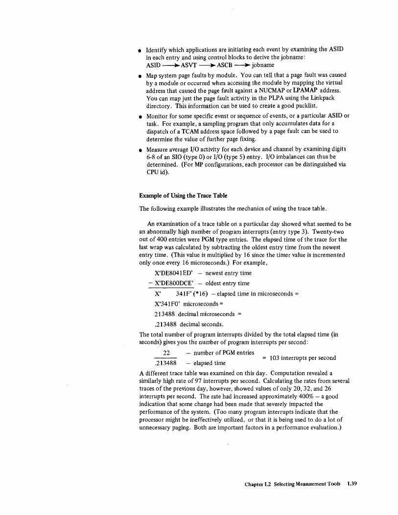
• Identify which applications are initiating each event by examining the ASID in each entry and using control blocks to derive the jobname: ASID ~ASVT ~ASCB ~ jobname
• Map system page faults by module. You can tell that a page fault was caused by a module or occurred when accessing the module by mapping the virtual address that caused the page fault against a NUCMAP or LPAMAP address. You can map just the page fault activity in the PLP A using the Linkpack directory. This information can be used to create a good packlist.
• Monitor for some specific event or sequence of events, or a particular ASID or task. For example, a sampling program that only accumulates data for a dispatch of a TCAM address space followed by a page fault can be used to determine the value of further page fixing.
• Measure average I/O activity for each device and channel by examining digits 6-8 of an SIO (type 0) or I/O (type 5) entry. I/O imbalances can thus be determined. (For MP configurations, each processor can be distinguished via CPU id).
Example of Using the Trace Table
The following example illustrates the mechanics of using the trace table.
An examination of a trace table on a particular day showed what seemed to be an abnormally high number of program interrupts (entry type 3). Twenty-two out of 400 entries were PGM type entries. The elapsed time of the trace for the last wrap was calculated by subtracting the oldest entry time from the newest entry time. (This value is multiplied by 16 since the timer value is incremented only once every 16 microseconds.) For example,
X'DE8041 ED' - newest entry time
- X'DE800DCE' - oldest entry time
X' 341 F' (* 16) - elapsed time in microseconds =
X'341FO' microseconds = 213488 decimal microseconds
.213488 decimal seconds.
The total number of program interrupts divided by the total elapsed time (in seconds) gives you the number of program interrupts per second:
22 - number of PGM entries
.213488 - elapsed time = 103 interrupts per second
A different trace table was examined on this day. Computation revealed a similarly high rate of 97 interrupts per second. Calculating the rates from several traces of the previous day, however, showed values of only 20, 32, and 26 interrupts per second. The rate had increased approximately 400% - a good indication that some change had been made that severely impacted the performance of the system. (Too many program interrupts indicate that the processor might be ineffectively utilized, or that it is being used to do a lot of unnecessary paging. Both are important factors in a performance evaluation.)
Chapter 1.2 Selecting Measurement Tools 1.39

An investigation into the changes made to the system since the previous day revealed that one of the steal algorithm constants in IRARMCNS (the SRM table) had been altered. It was hoped that this change would improve performance; in fact, it degraded it. By resetting the constant, program interrupts returned to their previous rate and overall performance was back to its original level.
Notes on Writing a Sampling Program
When writing a program to collect samples of the trace table, the following suggestions should be kept in mind:
• If you are using the trace table to look at a sequence of events, you must copy the entire table into storage without being interrupted. Although you can usually move the trace table without interruption, a good technique for assuring this is to save the current entry time before moving the table. (The current entry is pointed to by the first word in the header, which is pointed to by location X'S4'.) Then, after moving the table, compare the current entry time to the saved time. If the current entry time before and after the move is not the same, then the table was modified during the move. Throw the table away and start again. Do this sequence until the before and after times match; that is, until the table was not updated while being moved.
• When moving the table, copy the oldest part first followed by the newest. This results in a table of events in time-sequence order.
• You can copy the trace table into a larger area (a table with more than 32 bytes per entry) to provide space for other calculations and information accumulated by your program. For example, it might be helpful to include in the entry the time between successive events or the jobname associated with each event.
• Be sure you do not sample your own sampling program or a lot of useless data will be accumulated and analyzed.
SYSl.LOGREC
When gathering performance measurements, it is important that you also document the system environment that existed during the data collection period. A sophisticated analysis of seek activity on a DASD device is worthless unless you know what volume(s) was mounted on the device (information that is not provided in GTF records, for example). The SYSl.LOGREC data set, which provides a record of all hardware failures, selected software errors, and system conditions, is a valuable tool for this. It can also be useful as another source of performance data. Recoverable hardware and software errors that go unnoticed in a large complex might, in fact, be impacting overall system performance. Examples of performance-related data that can be recorded on the SYSl.LOGREC data set include the following:
• CCH records - contain information for every channel failure that does not terminate the system.
• DDR records - contain descriptions of operator and system swaps among the various devices.
• MCH records - contain information on processor, storage, storage key, and timer failures.
1.40 OS/VS2 MVS Performance Notebook
• OBR records - contain information on paging I/O errors and I/O device failures.
Each record'in SYS1.LOGREC contains error statistics for the device (counts of the number of times that channels, machine models, and I/O devices have failed) and environmental data (the time and circumstances for each failure or system condition). Hardware statistics can also be accumulated for buffered log devices.
The IFCEREPO service aid, which is used to retrieve the data from SYSI.LOGREC, reduces and formats the data as well. It enables you to examine the data in the form of edited reports, records, and/or record summaries such as the following:
• the IPL report - contains comprehensive information on the reasons for repeated system initializations, system idle time, and unavailability time.
• the system error report - contains error statistics for hardware or software failures.
The output from IFCEREPO should thus be considered an additional measurement tool when evaluating the performance of your system.
For more information on the contents and format of the SYSI.LOGREC data set (and the IFCEREPO service aid program), see OS/VS2 System Programming Library: SYS1.LOGREC E"or Recording.
Writing Data Reduction Programs
Your installation will need data reduction programs to summarize and format the data provided by the MVS components (SMF and GTF), the system trace table, and the performance-related control blocks. Data that can be derived from the trace table and the control blocks are described in the preceding topic, "Other Sources ofMVS Data." The SMF and GTF analysis programs, described in the "MVS Measurement Tools" section, are very useful reduction tools for the system components. These IBM-supplied programs summarize information from SMF and GTF that is often needed for a performance analysis. However, you might want to consider writing your own data reduction program in addition to, or in place of, any of those currently available. Your own program can measure variables that are pertinent to your particular installation's objectives and workload and might, therefore, require unique types of calculations.
This section provides general gUidelines on the key measurements to be extracted from SMF and GTF in order to do a meaningful performance evaluation. Only a subset of the data collected by these measurement tools is performance-related; thus, your data reduction programs should minimize overhead and simplify interpretation by producing only that information having immediate potential for performance analysis. This section will help you determine how you can use the data that you might want to collect. This should be decided first so that irrelevant records are not produced. The following basic steps should then be used to develop your program:
1. Read the SMF/GTF record.
2. Identify the type of record you are interested in via the record identifier or type fields.
Chapter 1.2 Selecting Measurement Tools 1.41
3. Write selected records to a workfile.
4. Sort and merge the selected records.
5. Analyze the sorted data to detect excessive system wait time, inefficient use of I/O devices, or any other statistics that might lead to improved system performance.
6. Format and print the selected data and summary statistics.
Reducing SMF Data
SMF produces the type of data that is needed to determine ajob's resource consumption; that is, almost all the data collected is job-related. SMF data is crucial for jobstream tuning, which in turn is essential to the good performance of a system. An additional advantage is that certain SMF data can be summarized on a job class and performance group basis. SMF data reduction programs should be written to match MF /1 or RMF intervals to get a complete picture of system workload. (See OS/VS2 System Programming Library: Initialization and Tuning Guide for examples of using these tools to compare an individual job's use of resources with that of the total system.)
The following discussion illustrates how SMF data can be used to measure system resources.
Measure where processor time is being spent. From records 5/35 and 4/34, obtain the processor time consumed by jobs and job steps. The processor time for each address space is broken down into execution time under TCBs and under SRBs. (See the topic "Categories of Processor Time" in chapter 11.2 for information on TCB and SRB time not reported by SMF.) Sort and summarize this data to determine which jobs are using large amounts of processor time. You can also focus on the specific elements of work that are using a lot of processor time by sorting the records by job or at the program level.
Measure storage usage to identify potential shortages and inefficient use. Detailed information about how storage is being used by different address spaces can be obtained from records 4/34. These records provide the number of page-ins, pageouts, swap-ins, and swap-outs. Reduction of this data will indicate which jobs are doing most of the swapping and paging and at what frequency.
From records 4/34, you can obtain the amount of virtual storage allocated and used by a job step or TSO session. These job step records can also be analyzed by your program to isolate the elapsed time and processor time used by job steps during the reporting pe~iod. The distribution of job steps in terms of storage used versus elapsed time or processor time can then be plotted. With this information, and the knowledge of how the jobs use the storage, you can identify the users and abusers of virtual storage. By translating the requests for virtual storage into their implications on real storage, and by knowing the storage size of the system, you will then be able to examine possible storage contention situations. A way to compute real storage from data in SMF records 4 and 34 is described in bulletin 4.2.0in chapter 11.4, under the topic, "Separating Users with Large Working Sets."
1.42 OS/VS2 MVS Performance Notebook

SMF data reduction programs can be written to combine information from the 4/34 records for job steps that overlap the same time interval. This data can be used to produce a report showing the storage utilization of the system at specific intervals. Specific periods of excessive storage waste and the jobs that caused it can thus be identified. This report will also indicate periods when there is low utilization of available storage.
Measure I/O a :tivity to determine the jobs that are using poor data management techniques (for example, blocking, MACRF, and RECFM). From records 14/15, obtain the following information in order to determine which data sets, if any, should increase their blocksizes, or otherwise improve their technique:
• the data set name
• the data set organization
• EXCP counts issued against the data set
• the blocksize of the data set
• record format of the data set
• macro form of the data set
• the ddname
• the jobname.
A reduction program, while extracting the data, can apply selection criteria to further simplify the analysis. For example, those data sets with less than a specified EXCP count can be ignored in order to obtain information on high usage data sets only. Another valuable indicator of the I/O activity of a job is its SRB time, since most SRB time is accumulated by I/O interrupt processing.
Measure system-wide resource activity. With a data reduction program, you can obtain from records 70-76 system-related data that was collected during an MF/l or RMF interval. Everything produced by MF /1 or RMF reports (processor, paging, workload, channel, and device activity) is provided in SMF records on an after-the-fact basis. For example, you can map the activity on all the channels and devices in use or only on specific ones to help determine where overloading situations have occurred. (For overall swap activity or swapping rates by performance groups, however, data contained in SMF records should be used with the rates provided by MF /1 or RMF; total swap counts produced by SMF can be misleading since swapping due to started or system tasks is not known to SMF.)
Reducing GTF Data
GTF, which traces system events, produces useful data for a performance analysis once it is reduced. In writing a data reduction program for GTF, remember that the format of GTF trace records depends on whether or not the record is timestamped. This is indicated by a bit in the Timestamp Control Record. GTF record formats and contents are described in OS/VS2 Service Aids Logic and OS/VS2 System Programming Library: Debugging Handbook.
Chapter 1.2 Selecting Measurement Tools 1.43
Much of the data provided by GTF that is relevant to performance measurements can be extracted and summarized using the analysis programs already mentioned (see figures 1.4 - 1.7). When writing your own reduction program, keep in mind the types of data that are provided by these programs. They may suggest several methods of sorting and analyzing the available data in order to obtain some meaningful measurements. Because of the potentially high overhead of running GTF, be selective in the options you specify.
The following discussion illustrates the major ways GTF data can be used to evaluate system resources.
Measure the processor time that is being spent on supervisor activity. Via sve trace records, GTF can identify the type, quantity, and users of supervisor services. Situations such as ENQ/DEQ bottlenecks can be determined by analyzing which services are in use, how they are being used, and by which jobs and modules. Focusing on the use of these services enables you to reduce processor bottlenecks, if necessary, by altering the time that an individual job spends on these services or by reducing the number of services that a job or jobs use during a period of time.
Analyze program activity for packlists and BLDL lists. Using the data from GTF, a reduction program can order the modules on these lists by frequency of use. Packlists, or BLDL lists (for non-reentrant modules), can be recreated to allow for more efficient use of the processor and I/O resources. Analyzing the page faults of modules can also result in the creation of a new packlist.
Measure I/O activity by device to obtain additional details. SIO and I/O trace records can provide information for each device such as the number of SIO operations, the extent of I/O interrupts, and the time intervals between SIOs. This can be very important when used with MF/l or RMF. For example, the MF /1 or RMF Device Activity Report might show a particular DASD device busy 75% of the time. By executing GTF and tracing the number of SIOs issued against the device, you can determine if there is a data set or VTOe placement problem. Since the SIO trace record contains the seek address from the DASD channel program, a reduction program can be used to illustrate graphically the nature of the seek activity on the busy volume. This graphic representation, when used with a LISTVTOe of the volume, can show that one or more data sets (or the VTOe) have been poorly placed on the volume. Based on this information, the data sets (or VTOe) can be rearranged on the pack for greater efficiency or can be redistributed to other, less active packs.
1.44 OS/VS2 MVS Perfonnance Notebook
Monitor SYSEVENT activity during a selected time interval. SRM trace records track each SYSEVENT macro that is issued; that is, a record is written whenever the status of an address space or a system resource has changed. Use the data to analyze the effect on system performance of critical changes to the availability of resources such as real storage frames, auxiliary storage slots, and SQA virtual space. To help interpret the data, your reduction program can sort these records by address space ID, sysevent type, or time of occurrence for each job or TSO session. Note that sysevent type 0 contains the TSO command or subcommand name in registers 15 and 1. For further information on the use of GTF to track sysevents, and examples on reducing data from the SRM trace records, see OS/VS2 System Programming Library: Initialization and Tuning Guide.
Monitoring Performance
It is important to keep in mind that tuning your system is an on-going process. Measurement tools should be executed on a regular basis, not only when performance problems become apparent. You should be able, once your objectives are met, to identify potential performance problems before they become crises.
Producing the same type of report or reports at periodic intervals should be a standard procedure at most installations. Data obtained in this way will enable you to determine the trends and the usual values for your particular installation. Once these values are established for individual workloads, you will be able to monitor performance. Any variation to the values usually observed can be indicative of a performance problem and warrants further investigation.
A measurement tool such as RMF can be run continuously with little degradation to the system's performance. Other tools, then, can be executed when RMF data indicates a potential problem area. The following are a few of the key measurements provided by RMF that should be examined regularly in order to monitor performance with maximum effectiveness:
• CPU Activity Report - wait time percentage.
• I/O Device Activity Reports - queue length and device busy percentages.
(Note, however, that since RMF overhead is directly related to the number of device classes monitored, you should specify only those devices that require monitoring.)
• Channel Activity Report - channel busy percentage (which provides feedback to the never-ending process of balancing DASD channel usage via data set and volume placement).
• Paging Activity Report - system and address space total swapping rate (auxiliary and real storage shortage swaps indicate inadequate paging space or an abnormal amount of system page fix activity); main storage frame count (deviations from the norm, such as a growth in the size of SQA, can be easily identified).
• Workload Activity Reports - all important data; especially useful for monitoring swapping and resource consumption on a performance group/ period/domain basis and for monitoring TSO response time.
Chapter 1.2 Selecting Measurement Tools 1.45

• Page/Swap Data Set Activity - PLPA and common slot usage (confirms that the page data set configuration is as desired; determines the page data sets where I/O errors are being encountered).
• Trace Activity - SRM trace; domain tables.
The SIR software monitor program is another possible tool for monitoring performance. It can assist you by identifying resource usage by individual jobs and address spaces.
1.46 OS/VS2 MVS Performance Notebook

Chapter 1.3 Pre-initialization MVS Performance Factors
In addition to defining performane objectives and ensuring needed measurement tools are available, the following performance-related areas must be addressed in planning for and generating a performance-conscious MVS system:
• the performance implications of the sysgen and initialization parameters you specify. The Initialization and Tuning Guide is the major source of information on this area .
• basic performance factors, which are applicable to all system control programs. This area was often ignored in early MVS systems and the following factors in particular should be carefully reviewed:
- the adequacy of the hardware configuration. Insufficient hardware will affect the performance of any system and MVS's utilization of some hardware resources differs from OS/MVT and VS2 SVS. Review the adequacy of the configuration, especially if the system was not upgraded for MVS -see the topic "Configuration" in Part III.
- I/O resource balancing~ I/O bottlenecks have been a significant source of processor wait time in several existing MVSsystems, yet this area of tuning is often ignored. Plan the configuration of I/O resources and data set placement carefully. Essentially, the rules that applied to MVT and SVS (such as placement of frequently used data sets near the VTOC) still apply to MVS. Chapter 11.3, "Investigating the Use of I/O Resources," in Part II describes measurements that can indicate possible I/O bottlenecks. Because of the dynamic nature of I/O requirements, I/O resource balanCing isan ongoing process and should be one of the major areas continuously reviewed as part of monit~ring performance.
- Users that monopolize system resources. A common performance-related axiom is that "10% of the users use 90% of the system" and the installation should identify and control these dominant users. If you isolate suspected dominant users in unique performance groups, RMF will report on the amounts of I/O, real storage, and processor service they use. SMF reports on virtual storage, processor, and I/O resources on a user level, but does not report on started tasks (you can also compute real storage on a User level from SMF data - see "Separating Users with Large Working Sets" in bulletin 4.2.0 in chapter 11.4). SIR reports on started tasks, but includes little data on the use of I/O resources. Using RMF, SIR, SMF, or similar tools - Or a combination of them - you can identify the dominant users at your installation. Control of dominant users depends on the user, its priority, and Similar installation-dependent factors. For example: if more than one batch job uses significant amounts of real storage, you can assign them to the same job class and assign that class to a single initiator, so they do not execute concurrently; or use the rotate priority for a group of jobs with ~eavy processor demands.
Operational bottlenecks. Operational bottlenecks can be a significant source of system degradation but often are ignored because they are not usually reflected in system measurements. More information on operational bottlenecks is provided below.
Chapter 1.3 Pre-initialization MVS Performance Factors 1.47

Operational Bottlenecks
In MVS, operators have a high degree of control over the system and their actions can seriously impact performance. For example, in MVT, an operator could start up to fifteen initiators; the number actually executed would depend on the amount of available storage. In MVS, if the operator starts fifteen initiators, all fifteen will attempt to run.
Education of the operators and early, active involvement of the operations staff in MVS installation planning are keys to avoiding operational bottlenecks. Tuning operational characteristics of the system can be more difficult than tuning components because of the human factor - it is more difficult to tune human beings. Conunents such as "I ran fifteen initiators on MVT" and "That's the way we did it on SVS" were common at some early MVS installations. Operators must understand basic MVS concepts and architecture in order to make intelligent decisions given a particular set of circumstances. Education of the operators is the most effective means of avoiding operational problems.
Operational bottlenecks that do occur are not obvious and often are not reflected in system measurements. For example, delays due to volume mounting are not usually reported by measurement tools because these delays occur before the EXCP and subsequent SIO are issued; MVS measurement tools report predominantly on the result of SIOs. Observation and awareness of common operational bottlenecks are the keys to recognizing operational bottlenecks. Before doing detailed performance analysis, you should check for operational bottlenecks - if they exist, but are ignored, the analysis can be long and futile. The following paragraphs describe some operational problems observed in existing MVS systems. Note that solutions to operational bottlenecks are often simplistic, but not necessarily simple to implement. For example, if delays occur in volume mounting or responding to WTOR requests, an obvious solution is to mount volumes and reply quickly. But implementing this solution will probably require more than a suggestion or an edict to the operators. You might review the adequacy of the operations staff or the effectiveness of their procedures to determine the cause of the delay - for example, excessive paperwork required of operators might be causing delays.
Number of Initiators
The n umber of initiators to run on MVS is not directly related to the number to run on SVS or MVT because of differences in system architecture. And the number of MVS initiators is very dependent on the environment. The operations staff should not determine the number of initiators to run or the job classes to be assigned to initiators. Recommended values for different shifts and different workloads should be determined by the system programmers and communicated to the operators. The operators should also be educated on the reasons behind the reconunended values; such education can help them withstand pressure from priority users complaining about their work. It has been observed that, when a user complains about ajob, the operator often responds by starting another initiator for that job class - often resulting in further system degradation.
1.48 OS/VS2 MVS Performance Notebook

Fonns Mounting
Potential problems in this area include jammed or empty printers and operators not responding to output-related messages (FCB loads, paper changes, and so on). To help avoid operational bottlenecks in forms mounting, reconsider the criteria for special forms and use JES2 and JES3 controls to group jobs with similar print req uirements.
Shift Changes
At some installations, operators quiesce the system to finish work on one shift before switching to the next shift. This can result in significant waste of system resources.
Input and Output
Turnaround time reported by system measurements will not include delays entering work into the system and delays distributing output. Be especially suspicious of this problem occurring if complaints of slow turnaround time occur predominantly for areas under control of separate operational groups - for example, specifically for locally-entered and distributed jobs.
Reply Delays
In addition to the simplistic solution of ensuring that WTOR requests receive responses quickly, you might want to examine and re-code applications that issue excessive WTORs. Old applications, written for earlier systems, often depend unnecessarily on the operator (for example, to supply time-of-day information).
Volume Mounting
In JES2, only jobs in execution can cause volume mounting. In JES3, volume mounting can delay the job in setup or, if mounts are issued after MAIN SELECT, during execution.
In addition to responding quickly to mount requests, you should consider controls for volume mounting. For example, you might examine the job mix and decide to run a large tape-spinning job on an off-shift. In JES3, the SDEPTH parameter might be too high for the number of initiators and tape drives in the system, reSUlting in tape drives being set up most of the time, although jobs using the drives have not been selected for execution. If a highpriority job enters the system, it might be necessary to restart setup to release needed tapes for higher-priority work. Watch for excessive restart setups, a long time spent on the main queue, a large number of jobs awaiting setup, and large fetch queue lengths.
Chapter 1.3 Pre-initialization MVS Performance Factors 1.49

1.50 OS/VS2 MVS Performance Notebook

PART II: Performance Analysis
Chapter 11.1: Steps in a Performance Problem Analysis
Chapter 11.2: Investigating the Use of Processor Time
Chapter 11.3: Investigating the Use of I/O Resources
Chapter 11.4: Investigating the Use of Real Storage
Chapter 11.5: User-oriented Performance Problem Analysis
Part II: Performance Analysis 11.1

11.2 OS/VS2 MVS Performance Notebook
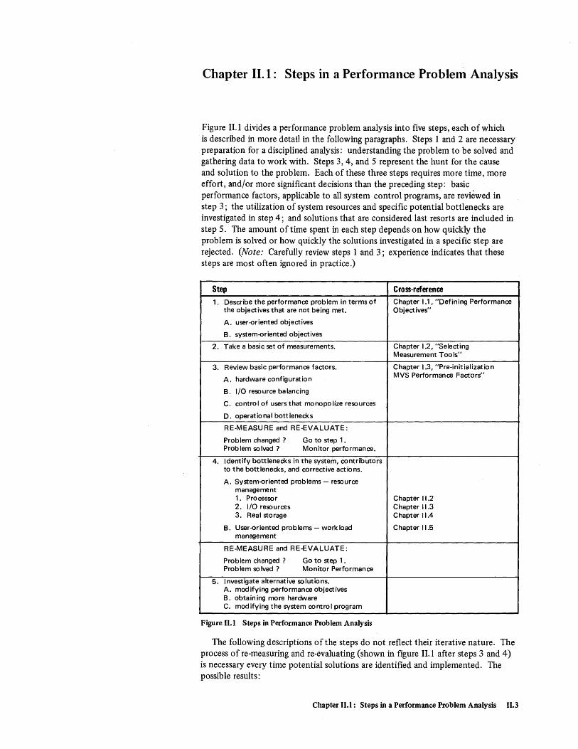
Chapter Ill: Steps in a Performance Problem Analysis
Figure 11.1 divides a performance problem analysis into five steps, each of which is described in more detail in the following paragraphs. Steps 1 and 2 are necessary preparation for a disciplined analysis: understanding the problem to be solved and gathering data to work with. Steps 3, 4, and 5 represent the hunt for the cause and solution to the problem. Each of these three steps requires more time, more effort, and/or more significant decisions than the preceding step: basic performance factors, applicable to all system control programs, are reviewed in step 3; the utilization of system resources and specific potential bottlenecks are investigated in step 4; and solutions that are considered last resorts are included in step S. The amount of time spent in each step depends on how qUickly the problem is solved or how quickly the solutions investigated in a specific step are rejected. (Note: Carefully review steps 1 and 3; experience indicates that these steps are most often ignored in practice.)
Step Cross-reference 1 . Describe the performance problem in terms of Chapter 1.1, "Defining Performance
the objectives that are not being met. Objectives"
A. user-oriented objectives
B. system-oriented objectives
2. Take a basic set of measurements. Chapter 1.2, "Selecting Measurement Tools"
3. Review basic performance factors. Chapter 1.3, "Pre-initialization
A. hardware configuration MVS Performance Factors"
B. I/O reso urce ba lancing
C. control of users that monopolize resources
D. operational bottlenecks
RE-MEASURE and RE-EVALUATE:
Problem changed ? Go to step 1. Prob lem so Ived ? Monitor performance.
4. Identify bottlenecks in the system, contributors to the bottlenecks, and corrective actions.
A. System-oriented problems - resource management 1. Processor Chapter 11.2 2. I/O resources Chapter 11.3 3. Real storage Chapter 11.4
B. User-oriented problems - workload Chapter 11.5 management
RE-MEASURE and RE-EVALUATE:
Problem changed ? Go to step 1. Problem solved? Monitor Performance
5. Investigate alternative solutions. A. modifying performance objectives B. obtaining more hardware C. modifying the system control program
Figure 11.1 Steps in Performance Problem Analysis
The following descriptions of the steps do not reflect their iterative nature. The process of re-measuring and re-evaluating (shown in figure 11.1 after steps 3 and 4) is necessary every time potential solutions are identified and implemented. The possible results:
Chapter 11.1: Steps in a Performance Problem Analysis 11.3

• The problem is solved and no new problems are jdentified; the analysis is completed.
• The immediate problem being addressed is solved but another problem becomes apparent. This is not unusual, because one bottleneck often disguises another. In this event, the analysis begins again with step 1.
• The problem remains and f~rther investigation is required; the analysis continues.
STEP 1. Describe the performance problem in terms of the objectives that are not being met.
The purpose of this step is to be as specific as possible in describing the performance problem(s). The problem description should include the extent of the problem (which will help you predict the effectiveness of possible solutions) and the specific type of work experiencing the problem (which will help you identify possible trade-offs). For example, "Fifty percent, as opposed to the desired ninety percent, of TSO trivial transactions during peak hours are receiving three second response time" is a good" problem description; "TSO is sluggish" is not.
Problem statements will be specific if your performance objectives were specific: gUidelines for defining performance objectives are included in Chapter 1.1. Two types of objectives, based on two types of measurements, were defined:
• user-oriented objectives - iresponse time for a specific class of transactions or turnaround time for a specific application or class of jobs; and
• system-oriented objectives - batch throughput, interactive transaction rate, or number of concurrent terminal users.
Note which type of objective is not being met in your system - it will affect the approach taken to identify bottlenecks, as described in step 4. If both uset~ oriented objectives and system-oriented objectives are not being met, investigate the system-oriented problems first.
11.4 OS/VS2 MVS Performance Notebook
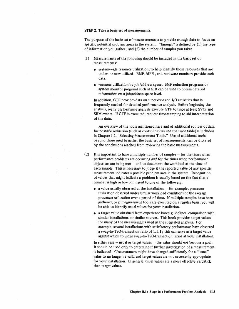
STEP 2. Take a basic set of measurements.
The purpose of the basic set 0 f measurements is to provide enough data to focus on specific potential problem areas in the system. "Enough" is defined by (1) the type of information you gather; and (2) the number of samples you take:
(1) Measurements of the following should be included in the basic set of measurements:
• system-wide resource utilization, to help identify those resources that are under- or over-utilized. RMF, MF /1, and hardware monitors provide such data.
• resource utilization by job/address space. SMF reduction programs or system monitor programs such as SIR can be used to obtain detailed information on a job/address space level.
In addition, GTF provides data on supervisor and I/O activities that is frequently needed for detailed performance analysis. Before beginning the analysis, many performance analysts execute GTF to trace at least SVCs and SRM events. If GTF is executed, request time-stamping to aid interpretation of the data.
An overview of the tools mentioned here and of additional sources of data for possible reduction (such as control blocks and the trace table) is included in Chapter 1.2, "Selecting Measurement Tools." Use of additional tools, beyond those used to gather the basic set of measurements, can be dictated by the conclusions reached from reviewing the basic measurements.
(2) It is important to have a multiple number of samples - for the times when performance problems are occurring and for the times when performance objectives are being met - and to document the workload at the time of each sample. This is necessary to judge if the reported value of any specific measurement indicates a possible problem area in the system. Recognition of values that might indicate a problem is usually based on the fact that a number is high or low compared to one of the following:
• a value usually observed at the installation - for example, processor utilization observed under similar workload conditions or the average processor utilization over a period of time. If multiple samples have been gathered, or if measurement tools are executed on a regular basis, you will be able to identify usual values for your installation.
• a target value obtained from experience-based gUidelines, comparison with similar installations, or similar sources. This book provides target values for many of the measurements used in the suggested analysis. For example, several installations with satisfactory performance have observed a swap-to-TSO-transaction ratio of 1.1: 1; this can serve as a target value against which to judge swap-to-TSO-transaction ratios at your installation.
In either case - usual or target values - the value should not become a goal. It should be used only to determine if further investigation of a measurement is indicated. Circumstances might have changed suffiCiently for a "usual" value to no longer be valid and target values are not necessarily appropriate for your installation. In general, usual values are a more effective yardstick than target values.
Chapter 11.1: Steps in a Performance Problem Analysis 11.5

Once a basic set of measurements has been taken, a major problem is determining which of those measurements to focus on. The analysis described in this Part of the Performance Notebook describes significant measurements to review in different situations.
STEP 3. Review basic performance factors, which are applicable to all system control programs.
The objective of this step is to ensure that basic tuning factors - those that are applicable to all system control programs - have been addressed before spending a lot of time and effort analyzing MVS specifically. The factors that should be addressed at this point have the following characteristics:
• The effect (positive or negative) of varying the factor is fairly predictable.
• The installation can easily exercise control over the factor - for example, via installation procedures or external system interfaces such as initialization parameters.
Based on experience with existing MVS systems, the following factors are important to consider at this stage:
• the adequacy of the hardware configuration in light of MVS system control program requirements.
• I/O resource balancing, achieved by data set placement and the configuration of channels, control units, and devices.
• control of users that monopolize system resources.
• operational bottlenecks.
These are the same factors that should be addressed prior to system generation and initialization - for details, see chapter 1.3, "Pre-initialization MVS Performance Factors;" the topic "Configuration-rules-of-thumb" in Part III includes guidelines against which you can review the adequacy of your configuration.
STEP 4. Identify and correct bottlenecks in the system.
This step represents the body of the analysis. The approach for identifying and correcting bottlenecks depends on the type of performance problem being experienced - whether system-oriented objectives or user-oriented objectives are not being met (see step 1). There are two major areas of control in the system: resource management and workload management. Although they overlap, the initial focus is on resources for system-oriented problems and on workload management for user-oriented performance problems.
11.6 OS/VS2 MVS Performance Notebook

In the case of a system-oriented problem, the goal is to identify the resources that could be used more effectively and to improve their use. The resources of the system can be reduced to five basic resources: the processor, real storage, channels, control units, and devices. Bottlenecks that affect throughput will affect one (or more) of these resources and be reflected in measurements of its use. The initial focus of the analysis is determined by answering the question, "Is the system waiting ?" System wait time is defined as processor-idle time and is reported on the RMF or MF /1 CPU activity report:
• If wait time is not high (for example, 10% or less of elapsed time), the analysis should focus on how processor time is being used, with the objective of reducing or eliminating non-productive processor time. This can lead to investigation of real storage, if significant processor time is being spent on paging or swapping; to investigation of I/O (with the intent of reducing EXCPs), if significant processor time is being spent on non-swap non-paging I/O interrupts; or to reduction of supervisor services such as SVCs. For details, see Chapter 11.2, "Investigating the Use of Processor Time."
• If wait time is high, you must determine why the system is waiting. Processor wait time is the result of four possible causes: (1) I/O delays; (2) eX'cessive paging; (3) enqueues on serially reusable resources and internal locks; or (4) insufficient work in the system. Assuming the last is not the problem, the most significant areas to investigate are I/O delays and excessive paging; significant sources of enqueue contention are often data sets (for example, catalogs), and this contention contributes to I/O delays. For information on investigating the possibility of I/O delays, see Chapter 11.3, "Investigating the Use of I/O Resources;" for the possible situation of paging causing wait time, see Chapter 11.4, "Investigating the Use of Real Storage."
Figure IL2 illustrates the logic of focusing on the major resources.
System-oriented problem identified
Invest igate use of processor time
activity report
Chapter 11.2
I/O delays: investigate use of I/O resources
Chapter 11.3
Excessive paging: investigate use of real storage
Chapter 1'.4
Figure 11.2 Focusing on the Major Resources when Investigating System-oriented Problems
Chapter 11.1: Steps in a Performance Problem Analysis 11.7

In the case of a user-oriented problem, the analysis has already focused on a specific application or class of jobs or interactive transactions. The goal is to determine why the work is being delayed -. to what resource(s)"it is not receiving access - and to increase its access to the needed resource(s). Increasing access to resources by the work in question usually implies trade-offs for other work in the system (that is, workload management). If such trade-offs cannot be tolerated, the analysis must focus on optimizing.use of the critical resource - that is, resource management. Chapter II.S describes the investigation of specific user-oriented performance problems.
STEP S. If performance problems are not solved in step 4, review alternative solutions: modifying performance objectives; obtaining more hardware; or modifying the system control program.
There is overlap between the steps of a performance analysis as outlined here. For example, any of these "alternative solutions" might have been identified in step 4 as the most effective solution to a bottleneck; the question of additional hardware resources might have been addressed in step 3, in reviewing the reasonableness of the current hardware configuration. The key to exploring these "alternative solutions" at any point in the analysis is the ability to predict the probability of meeting your objectives by means of other solutions - workload balancing, increasing resource utilization, decreasing unproductive resource usage, and so on. The formulas for reviewing hardware reasonableness (see the topic "Configuration - rules-of-thumb" in Part III) might indicate the necessity of modifying your objectives or obtaining more hardware. Detailed performance objectives (as described in Chapter 1.1) will allow you to identify minor changes to the objectives' priorities as solutions to resource bottlenecks identified in step 4. System modifications should be avoided. Before considering any system modification -or any solution - ensure it addresses a bottleneck identified in your system. There
; are no panaceas among the performance suggestions, despite the reputation of some. Each solution must be considered in light of your installation and its specific bottlenecks.
D.8 OS!VS2 MVS Performance Notebook

Chapter 11.2: Investigating the Use of Processor Time
Investigation of processor time should be triggered by the presence of high processor time (for example, greater than 90% of elapsed time); if processor time is not high, the primary focus of the analysis should be on decreasing processor wait time (see the description of step 4 and figure 11.2 in chapter ILl for information on the approach to performance analysis when processor wait time is high). There are essentially three ways to reduce the criticalness of the processor:
1. Identify and reduce or eliminate non-productive processor time.
2. If objectives still are not met and processor time is still high, focus on worklqad management: balancing the mix of processor- and I/O-bound jobs; rescheduling heavy processor users to less critical shifts. Note that, if you have defmed detailed performance objectives (including resource requirements - see chapter 1.1, "Defining Performance Objectives"), data will be available to help you determine effective workload changes.
3. If objectives still are not met and processor time is still high, consider alternative solutions: modifying the performance objectives; or a larger or additional processor.
This chapter describes the first approach: identifying and reducirig or eliminating non-productive processor time.
Identifying and Reducing Non-productive Processor Time
Identifying and reducing non-productive processor time involves dividing processor time into categories, measuring how much time is used in each category, and identifying those categories that might be reduced or eliminated for a positive effect on performance without an adverse effect on system functions.
Categories of Processor Time
Two rules dictate the choice of meaningful categories into which to divide processor time:
• The categories must be measurable - that is, the choice of categories depends on the measurement tools and reduction programs available at your installation .
• You must know what activities contribute to the processor time in each category.
Figure 11.3 illustrates various divisions of processor time and the overlap of different categories.
Chapter 11.2: Investigating the Use of Processor Time 11.9
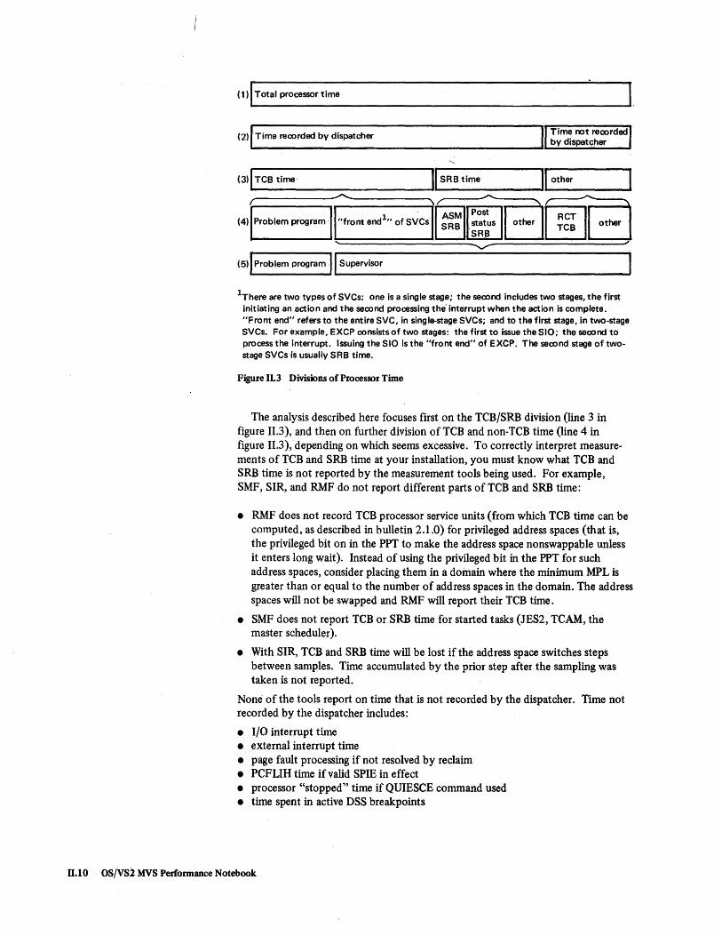
(1)ITotal processor time
(2) I Time recorded by dispatcher
(3)ITCB time'
r (4) Problem program·
./'0..-.... _____ __..
USRB time
Time not recorded by dispatcher
II other
---~ .... ---
I other'" ~~ I other
(5) Problem program. 1..1 s_u_pe_rv_iso_r __________________ -..,j
IThere are two types of SVCs: one is a single stage; the second includes two stages, the first initiating an action and the second processing the· interrupt when the action is complete. "Front end" refers to the entire SVC, in single-stage SVCs; and to the first stage, in two-stage SVCs. For example, EXCP consists of two stages: the first to issue the SIO; the second to process the interrupt. Issuing the SIO is the "front end" of EXCP. The second stage of twostage SVCs is usually SRB time.
Figure 11.3 Divisions of Processor Time
The analysis described here focuses first on the TCB/SRB division (line 3 in figure 11.3), and then on further division of TCB and non-TCB time (line 4 in figure 11.3), 'depending on which seems excessive. To correctly interpret measurements of TCB and SRB time at your installation, you must know what TCB and SRB time is not reported by the measurement tools being used. For example, SMF, SIR, and RMF do not report different parts ofTCB and SRB time:
• RMF does not record TCB processor service units (from which TCB time can be computed, as described in bulletin 2.1.0) for privileged address spaces (that is, the privileged bit on in the PPT to make the address space nonswappable unless it enters long wait). Instead of using the privileged bit in the PPTfor such address spaces, consider placing them in a domain where the minimum MPL is greater than or equal to the number of address spaces in the domain. The address spaces will not be swapped and RMF will report their TCB time.
• SMF does not report TCB or SRB time for started tasks (JES2, TCAM, the master scheduler).
• With SIR, TCB and SRB time will be lost if the address space switches steps between samples. Time accumulated by the prior step after the sampling was taken is not reported.
None of the tools report on time that is not recorded by the dispatcher. Time not recorded by the dispatcher includes:
• I/O interrupt time • external interrupt time • page fault processing if not resolved by reclaim • PCFLIH time if valid SPIE in effect • processor "stopped" time if QUIESCE command used • time spent in active DSS breakpoints
11.10 OS/VS2 MVS Performance Notebook

• ReT time • attention processing for TSO • page fault suspension processing • lock request suspension processing.
Also, measurements of TCB and SRB time will be inaccurate if the operator stops the processor from the console by pressing the STOP key. The TOD clock will continue to run and the time will be reported under the state the processor was running when it was stopped. To avoid this, use the QUIESCE command to stop the processor.
Focusing on Categories of Processor Time
Figure 11.4 illustrates the logic of focusing on different categories of processor time and includes cross-references to bulletins at the end of this chapter, which describe the investigation of specific categories.
The direction of the investigation is indicated by the proportion of processor time that is TCB time. The judgment of TCB time as "high" or "low" is installation-dependent and is best made in light of the proportion of TCB time usually observed at your installation. As a starting point for new installations, a target value of 50% (as measured by RMF, assuming that no address spaces are marked privileged in the PPT) might be used: if TCB time is greater than 50%, investigate it; ifless than 50%, determine the major areas of use of non-TCB time.
Processor busy time high. (e.g., > 90%)
No
Determine major areas of use of non-TCB time: • swapping • non-swap paging • I/O interrupts
Bulletin 2.2.0
Analyze SVCs
Bulletin 2.3.0
Identify heavy processor users.
Bulletin 2.4.0
Figure 11.4 Focusing on Categories of Processor Time
Chapter 11.2: Investigating the Use of Processor Time 11.11

Note that SRB time itself is not included in figure 11.4. ("Non-TeB time" includes reported SRB time and unreported processor time; much of the processor time used for swapping, paging, and I/O interrupts is unreported time.) SRB time is accumulated for services such as POST STATUS, cross-memory POST, crossmemory STATUS, the timing SRB, and the SRM timer pop SRB. Although it is possible to roughly determine hoY! much SRB time is being spent by the various services (using GTF and a nucleus map), it is not necessarily fruitful. It is not usually possible to reduce the processor time spent by most of these services: the effort of breaking down SRB time is not clearly justified by the possibility of the gain.
Additional bulletins on analyzing the use of processor time will be added as information becomes available.
11.12 OS/VS2 MVS Performance Notebook
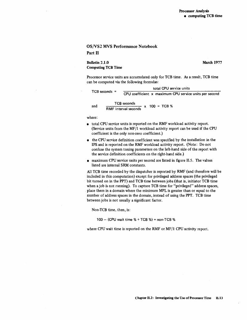
OS/VS2 MVS Performance Notebook
Part II
Bulletin 2.1.0 Computing TCB Time
Processor Analysis • computing TCB time
March 1977
Processor service units are accumulated only for TCB time. As a result, TCB time can be computed via the following formulas:
total CPU service units TCB seconds =
CPU coefficient x maximum CPU service units per second
and
where:
Tce seconds x 100
RMF interval seconds TCB%
• total CPU service units is reported on the RMF workload activity report. (Service units from the MF /1 workload activity report can be used if the CPU coefficient is the only non-zero coefficient.)
• the CPU service definition coefficient was specified by the installation in the IPS and is reported on the RMF workload activity report. (Note: Do not confuse the system tuning parameters on the left-hand side of the report with the service definition coefficients on the right-hand Side.)
• maximum CPU service units per second are listed in figure II.S. The values listed are internal SRM constants.
All TCB time recorded by the dispatcher is reported by RMF (and therefore will be included in this computation) except for privileged address spaces (the privileged bit turned on in the PPT) and TCB time between jobs (that is, initiator TCB time when a job is not running). To capture TCB time for "privileged" address spaces,
, place them in a domain where the minimum MPL is greater than or equal to the number of address spaces in the domain, instead of using the PPT. TCB time between jobs is not usually a Significant factor.
Non-TCB time, then, is:
100 - (CPU wait time % + TCB %) = non-TCB %
where CPU wait time is reported on the RMF or MF/l CPU activity report.
Chapter 11.2: Investigating the Use of Processor Time 11.13

Processor Analysis • computing TCB time
Bulletin 2.1.0 March 1977 Computing TCB Time (continued)
Note that this formula can also be used to determine rCB time for any of the distinct breakdowns of work reported in the RMF workload reports - performance groups, performance objectives, domains- by using the CPU service units for that group of work. For example, SMF does not report on started-task address spaces. You can use RMF to determine rCB time for started-task address spaces by assigning them to a separate performance group.
Processor Model Maximum CPU service units per second (assuming CPU coefficient of 1)
UP MP/AP
145 24.0
155 42.0
158 51.2 102.4
165 125.0
168 151.0 302.0
Figure 11.5 Maximum CPU Service Units per Second
11.14 OS/VS2 MVS Performance Notebook

OS/VS2 MVS Performance Notebook
Part II
Bulletin 2.2.0 Breakdown of non-TeB time
Processor Analysis • breakdown of non-TeB time
March 1977
Most processor time other than TCB time recorded by the dispatcher is due to swapping, I/O interrupts, and non-swap paging. The purpose of this bulletin is to help you determine the approximate percentage of processor time used for swapping, I/O interrupts, and paging - thereby identifying the area where further investigation might provide most Significant performance improvement. .
Figure 11.6 summarizes the formulas presented in this bulletin. The formulas for computing processor time for swapping, non-swap paging, and I/O interrupts are derived from the following formula for total non-TCB time, based on a 3.7 TSO and batch system with SUs 1-7 installed:
TCBol [51,000(SR) + 2,000(SPR) + 4,000(NSPR) + 2,000(SIOR)] x C,x 100 non- 10 ~ 6
10
where:
• SR is the swap rate - swaps per second, as reported in the swap sequence counts on the RMF paging activity report. 51,000 is the approximate processor time, in microseconds, for RCT (region control task) processing on a 158-3 UP.
• SPR is the swap paging rate - swap page-ins plus swap page-outs divided by the RMF interval in seconds, as reported on the paging activity report. 2,000 is the approximate processor time, in microseconds, for ASM (auxiliary storage manager) processing on a 158-3 UP, not including approximately 2,000 microseconds to process each I/O interrupt.
• NSPR is the total system non-swap paging rate - non-swap page-ins plus non-swap page-outs (including VIO, non-VIO, system areas, and private areas), divided by the RMF interval in seconds, as reported on the paging activity report. 4,000 is the approximate processor time, in microseconds, for ASM processing on a 158-3 UP, not including approximately 2,000 microseconds to process each I/O interrupt.
• SIOR is the SIOrate - total channel activity counts divided by the RMF interval in seconds, as reported by the channel activity report. 2,000 is the approximate time, in microseconds, for I/O-interrupt processing on a 158-3 UP.
• C is a coefficient that reflects the approximate relative time to perform systemcontrol-program (SCP) functions on various processors, as normalized to the 158-3 UP. (Therefore, for the 158-3 UP, Cis 1.0.) Figure 11.7 provides approximate coefficients for use in this formula.
Chapter 11.2: Investigating the Use of Processor Time 11.15

Processor Analysis • breakdown ofnon-TCB time
Bulletin 2.2.0 March 1977
Breakdown of non-TCB time (continued)
A. Basic formula for non-TCB %
[51,OOO(SR) + 2,OOO(SPR) + 4,OOO(NSPR) + 2,OOO(SIOR)] xC 100 non-TCB %~ 6 x
10
To check formula for non-TCB %:
result of formula A = non-TCB % from RMF (bulletin 2.1.0) (within R:S5%)
B. Formula for swap non-TCB %
C % [51,OOO(SR) + 2,OOO(SPR) + 2,OOO(SPR';" 3)J xC 100 swap non-T B 0 ~ x
106
assuming 3 pages per SIO.
C. Formula for non-swap paging non-TCB %
. Tca % "'-J [4,OOO(NSPR) + 2,OOO(NSPR';- 2)J xC 100 non-swap paging non- O"'-J x
106
assuming 2 pages per SIO.
D. Formula for non-swap non-paging I/O interrupt non-TCB %:
non-swap non-paging I/O interrupt non-TCB % ~
[2,OOO(SIOR - (SPR';- 3) - (NSPR';' 2))J x C x 100
106
which excludes I/O interrupts for non-swap paging and swapping, assuming 3 pages per SIO for swapping and 2 pages per SIO for non-swap paging.
Legend: SR = swap rate SPR = swap page rate NSPR = non-swap page rate SIOR = SIO rate
Figure 11.6 Formulas for Breakdown of non-TCB Processor Tjrne
From experience to-date, this formula is accurate within approximately 5%. However, the times for RCT, ASM, and I/O-interrupt processing on a 158-3 UP, and the coefficients reflecting the relative time to process these functions on different processors, are approximations and can vary significantly from the values given. As a result, it is imperative to check the result of the preceding formula. Compare the result of this formula to the non-TCB percentage computed via RMF (assuming no address spaces are marked privileged in the PPT, so that all TCB time recorded by the dispatcher is reflected in RMF measurements - see Bulletin 2.1.0). If the results differ by more than 5%, the fault might lie with an unusual activity in your system that is consuming processor time. Review system activity at the time of the report. For example, in one case where this formula seemed incorrect, an excessive number of nonswappable address spaces were active in the system. The dispatcher was "tripping" over them on the dispatching queue and dispatcher processor time had increased dramatically.
11.16 OS/VS2 MVS Performance Notebook

Processor Analysis • breakdown of non-TeB time
Bulletin 2.2.0 March 1977 Breakdown of non-TeB time (continued)
Processor Model Approximate Coefficient
!!.!!!!E These coefficients are approximations, based on measurements of system-control-program (SCP) functions in certain jobstreams that reflect common user environments, and normalized to a 158-3 UP; the jobstreams were executed on an MVS release 3.7 system with SUs 1-7 installed. The coefficients do vary and, therefore, results of any formulas using these coefficients must also be con-sidered approximations. These approximate coefficients apply only to SCP functions; they should not be used for comparing non-SCP programs on different processors.
145 2.60 155 1.46
158 UP 1.11 158 MP .67 158-3 UP 1.00 158-3 AP/Mp .59
165 .52
168 UP 8K cache .47 168 UP 16K cache .42 168 half-duplex 16K cache .43 168 MP .274
168-3 UP .36 168-3 half-duplex .37 168-3 AP/MP .213
Figure 11.7 Coefficients Reflecting Relative Time to Perform SCP Functions on Different Processor Models
If the result of this formula seems correct (that is, within approximately 5% of other computations of non-TCB time), the following formulas can be used to compute approximate non-TCB time used for swapping, non-swap paging, and I/O interrupts:
• swapping non-TCB % :::::s
[51,000(SR) + 2,000(SPR) + 2,000(SPR - 3)] x e lx 100
106
where (SPR+ 3) reflects the number of SIOs, assuming three pages for each SIO.1 The assumption of 3 pages per SIO is based ·on a working set ,size of 12 pages, five of which are LSQA; and four local paging data sets on 3330 devices. The number of pages per SIO will tend to increase if: the working set is larger; page data sets are on a drum; the swap load is very heavy (it is more likely that as many pages as possible will be swapped in/out in each ASM burst); or the ASMBURST value is raised by the installation. The number of pages per SIO will tend to decrease if more local page data sets are added or if the ASMBURST value is lowered by the installation.
11f all paging data sets are dedicated, the average number of pages per 510 for swapping and non-swap paging combined is:
total paging rate
sum of paging devices' activity counts per second
Chapter 11.2: Investigating the Use of Processor Time 11.17

Processor Analysis • breakdown of non-TCD time
Bulletin 2.2.0 March 1977 Breakdown ofnon-TCB time (continued)
If swapping processor time is judged excessive, the solution is to reduce swapping - see bulletin 4.1.0 in the chapter, "Investigating the Use of Real Storage."
• non-swap paging non-TCB % ~
[4,000(NSPR) + 2,000(NSPR .;.. 2)J x c ---------------" x 100
106
where (NSPR ~ 2) reflects the number of SIOs,assuming two pages per S10.1
The number of non-swap pages, per SIO varies with the amount of VIO and demand paging. As VIO and demand paging increase, the number of pages per SIO increases up to the maximum that can be handled in a single ASM burst (a probable maximum of 5 on a 3330 and 10 on a 2305 during a 50-millisecond burst). The assumption of 2 pages per SIO is based on the paging data sets being on 3330s.
If non-swap paging processor time is judged excessive, compare non-VIO and VIO paging rates to determine where decreases will potentially have the more significant effect. Bulletins 4.2.0 and 4.3.0 in chapter 11.4 describe decreasing demand paging and VIO paging, respectively.
• non-swap non-paging I/O interrupt non-TCB % ~
2,000[(SIOR - (SPR .;.. 3) - (NSPR';'-2))J x c 6 x 100
10
This formula excludes processor time used for I/O interrupts for non-swap paging and swapping (based on the preceding assumptions of 3 pages per SIO for swapping and 2 pages per SIO for non-swap paging). If I/O interrupt processor time is judged excessive, the solution is to reduce the number of EXCPs/SIOs - see bulletin 3.4.0 in the chapter 11.3, "Investigating the Use of
" I/O Resources."
Figure 11.8 is an example of applying the formulas presented in this bulletin.
Ilf all paging data sets are dedicated, the average number of pages per SIO for swapping and non-swap paging combined is:
total paging rate
sum of paging devices' activity counts per second
11.18 OS!VS2 MVS Performance Notebook

Processor Analysis • breakdown of non-TCB time
Bulletin 2.2.0 March 1977 Breakdown of non-TCB time (continued)
System: 158-3 UP 3 meg MVS 3.7 with SUs 1-7 and RMF applied. TSO and batch
Computing TCB time via RMF:
Data
CPU busy = 100 - 3.14 = 96.86% total CPU service units = 1,057,298 CPU coefficient = 10.0 maximum CPU service units/second = 51 .2 interval = 60.12.862 = 3612.86 seconds
TCB seconds = 1,057,298 2065.04 51.2 x 10
TCB % = 2065.04 x 100 = 57.16% 3612.86
non-TCB % = 96.86 - 57.16 = 39.70%
Formula for non-TCB time:
Data
Source
CPU activity report work load activity report work load activity report figure 11.5 work load activity report
Source
SR = 1.49 RMF paging activity report SPR = 23.91 + 21.46 = 45.37 RMF paging activity report NSPR = 16.15 + 3.60 = 19.75 RMF paging activity report SIOR = 323,492+3612.86 = 89.54 RMF channel activity report C = 1.0 Figure 11.7
TCB 011"1[51,000(1.49) + 2,000(45.37) + 4,000(19.75) + 2,000(89.54)] x 1.0
non- 101"1 ·x 100 . 106
~42.48%
Testing formula for non-TCB time:
42.48 - 39.70 = 2.78% (within 5%)
Formula for swapping non-TCB %:
. TCB 01 1"1,[51,000(1.49) + 3,000(45.37) + 2,000(45.37';" 3)] X 1.0 100 swappmg non- 10 '" . . x
106
~19.70%
Formula for non-swap paging non-TCB %:
. Tce OL 1"1[4,000(19.75) + 2,000(19.75";- 2)] x 1.0 non-swappagmg non- /oI"IX 100
106
~9.88%
Formula for non-swap non-paging I/O interrupt non-TCB %:
I/O . TCB 01 [2,000(89.54 - (45.37";' 3) - (19.75';- 2))] x 1.0 Interrupt non- 10 ~ .... x 100
106
~12.91%
Figure 11_8 Example of Applying Formulas for Breakdown of non-TCB Time
Chapter 11.2: Investigating the Use of Processor Time 11.19

11.20 OS!VS2 MVS Performance Notebook
OS/VS2 MVS Peformance Notebook
Part II
Bulletin 2.3.0 SVC analysis
Processor Analysis • SVC analysis
March 1977
The purpose of analyzing SVCs is to identify those SVCs that are "costly" in terms of processor time and whose "cost" can be decreased - by decreasing the frequency of the sve or by reducing the SVC's processor time. The factors important in identifying such SVCs are:
• Recognition of SVCs whose operation or frequency can be changed without having an adverse effect on system functions. The topic "SVCs" in Part III presents suggestions on redUCing the frequency or processor usage of some SVCs.
• The frequency of SVCs, available by trace table or GTF analysis. GTFSVC, IUP # 5796·PGE, is a GTF reduction program that provides SVC frequency on a system and job level. To use frequency to focus on specific SVCs, you should have a fairly clear idea of SVC frequencies u~ually observed in your system when performance objectives are being met. SVCs cannot be judged only by relative frequency, since relative frequency does not equate to relative processor cost; ten calls of one SVC can equal, in terms of processor time, one call of another, However, since it is not Simple to determine relative processor cost of the SVCs (which is the third factor in SVC analysis), frequency is often used as an inexact indicator.
• The processor time used by SVCs. Although the process is involved, this can be compllted using GTF or the trace table. The following paragraphs describe a method for doing this.
Computing Relative Processor Cost of SVCs
Computing the processor cost of SVCs is based on measuring the TeB seconds spent executing each SVC, which is not a trivial task. To determine the TeB time for each SVC, use GTF or trace table data to obtain:
1. The total TCB time spent executing each SVC (all calls of the SVC). Each time an SVC is issued by each task in the system, take the difference from the time the SVC starte<;l to redispatch of the task. If the task is interrupted, the time between the interrupt and reinstatement of the task must be subtracted from the SVC execution time. Note also that an SVC can call one or more additional SVCs. The time spent executing the "nested" SVCs should be included in the processor time of the base SVC, although you might also want to report TeB time for the nested SVCs individually.
Chapter 11.2: Investigating the Use of Processor Time 11.21
Processor Analysis • sve analysis
Bulletin 2.3.0 March 1977 sve analysis (continued)
2. The average time spent executing each call of the SVC, by dividing the total TCB time spent executing the SVC by the frequency of that sve in the sample period. The TeB time of each call of an SVC will vary; in some cases, this variance will be significant enough that the average TCB seconds for that SVC might be meaningless, unless a great number of samples are used.
(Note that a less exact, but simpler, way of obtaining relative size of SVCs is to track the elapsed time of each SVC - from the time the SVC is issued until redispatch of the task, which does not take into account factors such as interruption of the task.) Once the average TCB time for each SVC is known for your system, you can determine the processor "cost" of each SVC for any given measurement interval as a percentage of total processor utilization or as a percentage of total TCB time:
SVC A's TCB % of processor utilization ~
avg. TCB seconds for SVC A x frequency per second of SVC A x 100'
processor utilization
SVC A's % of total TCB time ~
avg. TCB seconds for SVC A x frequency per second of SVC A x 100
total TCB %
where frequency per second for the period of time being investigated can be determined by GTF analysis, trace table analysis, or obtained from GTFSVC (IUP #5796-PGE); and processor utilization or total TCB % is expressed as a fraction.
Note that, if your installation includes more than one type of processor, you can use the coefficients in figure II.7 (included in bulletin 2.2.0) to convert SVC time measured on one processor to the approximate SVC time on a different processor:
TCB seconds for SVC A ~ C2 x TCB seconds for SVC A
C1 where C1 is the coefficient of the processor on which the SVCs were measured and C2 is the coefficient of the processor on which you are projecting SVC time.
11.22 OS/VS2 MVS Performance Notebook
Bulletin 2.3.0 sve analysis (continued)
Processor Analysis • SVC analysis
March 1977
Figure 11.9 is an example of average TeB processor microseconds measured for SVCs on a 168-3 half duplex (HD) 6 meg TSO and batch system (approximately 90% TSO, 10% batch) with processor utilization of 88%, computed by means of trace table reduction. The last column in figure 11.9 illustrates converting the average times measured on the 168-3 HD to the approximate average times the SVCs would take on a 158-3 UP. (Some performance analysts find the 158-3 UP base numbers to be the most convenient form in which to use the values.) The formula used for the conversion, using the coefficients for the 158-3 UP and the 168-3 HD from figure 11.7, is:
average TCB seconds for SVC A on 158-3 UP ~
1.0 x avg. TCB seconds for SVC A on 168-3 H D
.37
Figure 11.9 illustrates the possible wide variance in processor time spent by SVCs, in relation to their frequency. For example, computing TCB % of processor utilization for SVCs 0 (EXCP/XDAP) and 10 (GETMAIN/FREEMAIN) on the 168-3 HD (where the microseconds, taken from figure 11.9, have been converted to seconds and processor utilization was 88%):
• SVC 0 TCB % = .000788 x 93.4 x 100 = 8.36%
.88
• SVC 10 TCB % = .000238 x 232.2 x 100 = 6.28%
.88
Although SVC 10 was executed two-and-a-half times more frequently than SVC 0 (232.2 versus 93.4 calls per second), SVC 0 accounted for 33% more TCB processor time. Also, SVC 0 is a two-stage SVC and the TCB time is only the "front end;" approximately the same amount of processor time (SRB time) is spent in the second stage of the SVC, fielding the interrupt.
Figure 11.9 is included only as an example. The average TCB microseconds listed can vary significantly from those at your installation.
Chapter 11.2: Investigating the Use of Processor Time 11.23

Processor Analysis • SVC analysis
Bulletin 2.2.0 March 1977 SVC analysis (continued)
Warning: This figure is included only as an example. The average TCB time spent executing an SVC depends significantly on the characteristics of the workload being supported; the times listed in this figure can .vary significantly from those at your own installation. Also note that:
• the lower the frequency of the SVC, the greater the possible distortion in its computed average TCB time.
• the observed frequency includes all SVCs that were issued during the time of the trace table sample; however, computation of average TCB time is based only on SVCs that were issued and completed within the time of the trace table sample.
System Level: 168-3 half-duplex (HD) 6 meg TSO (~90%) and batch (~10%) MVS Release 3.7 with RMF, RACF, TSO Command Package, NJE Facility for JES2, and the following SUs installed: 1,2,4,5,6,7,8,10,15
Average TC B Microseconds (including TCB time of other
Average TCB Microseconds SVCs called by base SVC) Observed Frequency (including TC B time of other on 158·3 UP, Converted (per second) on SVCs called by base SVC) from Times Measured on
SVC No. SVC Name 168·3 HD Measured on 168·3 HD 168·3 HD
0 EXCP/XDAP 93.4 788 2130 1 WAIT/WAITR 93.0 199 538 2 POST/PRTOV 5.1 182 492 3 EXIT 15.8 (see note 1) 4 GETMAIN 6.3 343 927 5 FREEMAIN .7 431 1165 6 LINK 1.9 (see note 2) 7 XCTL 4.1 376 1016 8 LOAD 7.5 490 1324 9 DELETE 14.0 250 676
10 GETMAIN/FREEMAIN 232.2 238 643 11 TIME 7.3 122 330 12 SYNCH 4.3 (see note 2) 13 ABEND/(EOT) 0 9200* 24865 14 SPIE 0 943* 2549 15 ERREXCP .1 176 476 16 PURGE 3.7 6786 18341 17 RESTORE 0 18 BLDL/FIND 4.1 2739 (see note 3) 7403 (see note 3) 19 OPEN .7 10710 28946 20 CLOSE 1.7 1709 4619 21 STOW 0 22 OPEN (TYPE=J) .3 8335 22527 23 CLOSE (TYPE=T) .1 9638 26049 24 DEVTYPE .1 303 819 25 TRKBAL .1 336 908 26 CA T A LOG/I N DEX/LOCATE 1.3 10403* 28116 27 OBTAIN .3 4357* 11776
*These_ WArA frnrn '" .'~ .. "'" .... 1 .. ; • +I..·s sample, the +GB time was---ftOt-eaptttr"",..." ... '" L·, .. '1 ...... "Y uf the SVC was zero.
Notes: 1. EXIT does not return to the next sequential instruction; EXIT is included in the SVC that issues the EXIT. 2. According to the technique used, time spent executing the linked or synched program would have been counted as part of
this SVC. As a result, no time was computed for LINK or SYNCH. 3. The processor time of BLDL varies widely according to the amount of I/O done.
Figure 11.9 Example of Average TCB Times for SVCs on a 168·3 6 Meg TS.o and Batch System (part 1 of 4)
11.24 OS/VS2 MVS Performance Notebook

Bulletin 2.2.0 SVC analysis (continued)
Processor Analysis • SVC analysis
March 1977
Warning: This figure is included only as an example. The average TCB time spent executing'an SVC depends significantly on the characteristics of the workload being supported; the times listed in this figure can vary significantly from those at your own installation. Also note that:
• the lower the frequency of the SVC, the greater the possible distortion in its computed average TCB time .
• the observed frequency includes all SVCs that were issued during the time of the trace table sample; however, computation of average TCB time is based only on SVCs that were issued and completed within the time of the trace table sample.
System Level: 168-3 half-duplex (HD) 6 meg TSO (~ 90%) and batch ( ~ 10%) MVS Release 3.7 with RMF, RACF, TSO Command Package, NJE Facility for JES2, and the following SUs installed: 1, 2,4, 5, 6, 7, 8, 10, 15
Average TCB Microseconds
Average TCB Microseconds (including TCB time of other SVCs called by base SVC)
Observed Frequency (including TC B time of other on 158-3 UP, Converted (per second) on SVCs called by base SVC) from Times Measured on
SVC No. SVC Name 168-3 H 0 Measured on 168-3 H 0 168-3 HD
28 CVOL 0 29 SCRATCH .1 1902* 5141 30 RENAME 0 31 FEOV 0 32 [no name] .1 1324* 3578 33 IOHALT 0 34 MGCR/OEDIT .1 2941 7949 35 WTO/WTOR .3 3612 9762 36 WTL .3 1686 4557 37 SEGLD/SEGWT 0 38 [reserved] 39 LABEL 0 40 EXTRACT 2.5 130 351 41 IDENTIFY .1 431 1165 42 ATTACH .3 919 2484 43 CIRB 0 44 CHAP 0 45 OVLYBRCH .7 5435 14689 46 TTIMER 0 47 STIMER .7 827 2235 48 DEO 23.8 290 784 49 [reserved] 50 [reserved] 51 SNAP/SDUMP 0 52 RESTART 0 53 RELEX 0 54 DISABLE 0 55 EOV 1.5 2155 5824 56 ENO/RESERVE 26 336 908 57 FREEDBUF 0 58 RELBUF/REOBUF 0 59 OLTEP 0 60 STAE/STAI/ESTAE/ESTAI 40.6 123 332 61 IKJEGS6A 0 62 DETACH .5 213 576 63 CHKPT 0 64 RDJFCB 0 65 [reserved]
*These numbers were obtained from a different sample; in this sample, the TCB time was not captured or the frequency of the SVC was zero.
Figure 11.9 Example of Average TCB Times for SVCS on a 168-3 6 Meg TSO and Batch System (part 2 of 4)
Chapter 11.2: Investigating the Use of Processor Time 11.25

Processor Analysis • SVC analysis
Bulletin 2.2.0 March 1977 SVC analysis (continued)
Warning: This figure is included only as an example. The average TCB time spent executing an SVC depends significantly on the characteristics of the workload being supported; the times listed in this figure can vary significantly from those at your own installation. Also note that:
• the lower the frequency of the SVC, the greater the possible distortion in its computed average TCB time.
• the observed frequency includes all SVCs that were issued during the time of the trace table sample; however, computation of average TCB time is based only on SVCs that were issued and completed within the time of the trace table sample.
System Level: 168-3 half-duplex (HD) 6 meg TSO ( ~ 90%) and batch (~ 10%) MVS Release 3.7 with RMF, RACF, TSO Command Package, NJE Facility for JES2, and the following SUs installed: 1,2,4,5,6,7,8,10,15
Average TC B Microseconds (including TCB time of other
Average TCB Microseconds SVCs called by base SVC) ObselVed Frequency (including TCB time of other on 158-3 UP, Converted (per second) on SVCs called by base SVC) from Times Measured on
SVC No. SVC Name 168-3 HD Measured on 168~3 HD 168-3 HD
66 BTAMTEST 0 67 68 SYNADAF/SYNADRLS 0 69 BSP 0 70 GSERV 0 71 ASGNBFR/BUFINO/RLSEBFR 0 72 CHATR 2.9 1413 3819 73 SPAR 0 74 DAR 0 75 DaUEUE 0 76 [no name] 0 77 [reserved] 78 WSCAN 0 79 STATUS 25.4 141 381 80 [reserved] 81 SETPRT 0 82 DASDR 0 83 SMFWTM 3.1 4494 12146 84 GRAPHICS 0 85 DDRSWAP 0 86 ATLAS 0 87 DOM 0 88 MOD88 0 89 [reserved] 90 [reserved] 91 VOLSTAT 0 92 TCBEXCP 0 93 TGET/TPUT 3.3 687 1857 94 STCC .1 400 1081 95 SYSEVENT 8.1 260 703 96 STAX .9 137 370 97 TEST-TSO .1 495 1338 98 PROTECT 0 99 DDDYNAM 2.1 11476 31016
100 IKJEFFIB 0 101 OTIP 4.7 408 1103 102 AOCTL 0 103 XLATE 0
Figure 11.9 Example of Average TCB Times for SVCs on a 168-3 6 Meg TSO and Batch System (part 3 of 4)
11.26 OS!VS2 MVS Performance Notebook

Bulletin 2.2.0 SVC analysis (continued)
Processor Analysis • SVC analysis
March 1977
Warning: This figure is included only as an example. The average TCB time spent executing an SVC depends significantly on the characteristics of the workload being supported; the times listed in this figure can vary significantly from those at your own installation. Also note that:
• the lower the frequency of the SVC, the greater the possible distortion in its computed average TCB time .
• the observed frequency includes all SVCs that were issued during the time of the trace table sample; however, computation of average TCB time is based only on SVCs that were issued and completed within the time of the trace table sample.
System Level: 168-3 half-duplex (HD) 6 meg TSO (~90%) and batch (~10%) MVS Release 3.7 with RMF, RACF, TSO Command Package, NJE Facility for JES2, and the following SUs installed: 1, 2, 4, 5,6, 7, 8, 10, 15
Average TC B Microseconds (including TCB time of other
Average TC B Microseconds SVCs called by base SVC) Observed Frequency (including TCB time of other on 158·3 UP, Converted (per second) on SVCs called by base SVC) from Times Measured on
SVC No. SVC Name 168-3 HD Measured on 168·3 HD 168-3 HD
104 TOPCTL 0 105 IMAGLIB 0 106 107 MODESET
(/& .5 80 216
108 [reserved] 109 ESR (type 3 & 4) .7 391 1057 110 DSTATUS 0 111 [calls HASPSSSM] 4.3 1102 2978 112 PGRLSE 0 113 PGFIX/PGFREE/PGLOAD/ 5.9 280 757
PGOUT 114 EXCPVR 2.7 460 1243 115 [reserved] 116 ESR (type 1) 2.1 78 211 117 DEBCHK 10.5 108 292 118 [reserved] 119 TESTAUTH .9 54 146 120 GETMAIN/FREEMAIN 20.4 181 489 121 VSAM 3.1 911 2462 122 ESR (type 2) 0 123 PURGEDQ 5.5 582 1573 124 TPIO 4.9 175 473 125 EVENTS 0 126 [no name] 130 RACHECK 0 131 RACINIT .1 1662 4492 132 RACF manager 0 133 RACDEF 0
Figure 11.9 Example of Average TCB Times for SVCs on a 168·3 6 Meg TSO and Batch System (Part 4 of 4)
Chapter 11.2: Investigating the Use of Processor Time 11.27

11.28 OSjVS2 MVS Performance Notebook

OS/VS2 MVS Performance Notebook
Part II
Bulletin 2.4.0 Identifying heavy processor users
Processor Analysis • identifying heavy processor users
March 1977
To solve processor (or any other resource) constraints, it is often necessary to address the dominant address spaces. Figure 11.10 summarizes the steps described in this bulletin for focusing on heavy processor users.
SMF provides TCB and SRB time for jobs and logons in the type 5 and 35 records, respectively. Focus on those jobs with the highest TCB time. On a lower level, you can identify the programs and commands that use high TCB time. SMF provides TCB and SRB time by program in the type 4 (step termination) record. Similar information on a command basis is not automatically provided. However, if PCF (Programming Control Facility, FDP # 5798-BBJ) is included in the system, it can be used to selectively trace commands and to obtain an SMF record for commands similar to the type 34 record for TS-step termination.
TCB time consists essentially of SVC time and problem program time. You can identify the SVCs called by a particular job/logon using GTF or the trace table. GTFSVC (IUP # 5796-PGE, a GTF reduction program) provides SVC information on a "job" basis, where job refers to the jobname field in the GTF trace record and therefore includes batch jobs, TSO user sessions, the master scheduler, JES2, TCAM, etc. The job detail report further divides SVC usage for a particular job by TCB address, module name, and PSW address. Note, however, that no known IBM-provided tool reports SVC information on a program or command basis unless the program or command equates to a module name(s).
Using GTFSVC, you can focus on jobs with high percentages of SVC activity and then identify the particular SVCs used by those jobs. To judge the usage of the specific SVCs requires knowledge of SVC usage you would expect to see, of SVCs whose usage might be decreased without an adverse effect on function, and of SVCs that are costly in processor time.
Determining relative processor cost of SVCs is not trivial; a method to do so, based on determining the average T~B seconds spent executing each SVC, is described in bulletin 2.3.0. If you have determined average TCB seconds for each SVC, you can compute approximate SVC time for a particular job via the following formula:
SVC TCB time for job A ~
255 ~
n=O (SVC n frequency by job A x avg. TCB seconds for SVC n)
Chapter 11.2: Investigating the Use of Processor Time 11.29

Processor Analysis • identifying heavy processor users
Bulletin 2.4.0 March 1977 Identifying heavy processor users (continued)
STEP Tool or cross·reference
1. Identify users with relatively high TCB time. SMF records 5 and 35
2. Identify programs or commands with relatively programs: SMF record 4
high TCB time. (Note, however, that no known commands: PCF (FOP #5798-BBJ) IBM-provided tool provides SVC information on a program or command basis unless the program or command equates to a module name(s).)
3. Identify jobs with high SVC activity. GTF or trace table analysis; GTFSVC (I UP #5796-PGE)
4. Focus on SVC part of TCB time for jobs identified via steps 1 and 3.
5. Determine frequency of SVCs in jobs focused on. Judge usage of SVCs, based on:
• expected or usual usage of SVCs by the work in question.
• SVCs that can be changed or whose topic "SVCs" in Part III frequency can be reduced without an adverse effect on function.
• relative processor cost of SVCs GTF or trace table reduction - see bulletin 2.3.0
6. If relative processor cost of SVCs is computed: GTF or trace table reduction - see
• determine SVC TCB % for jobs being bulletin 2.3.0
investigated; subtract from total TCB time for job to obtain approximate problem program time.
• if problem program time is unusually high for type of application, examine program design.
• compute TCB time for particular SVCs Us.9d by the job and focus on those SVCs that account for significant proportion of total job TCB time.
Figure 11.10 Steps In Focusing On Heavy Processor Users
11.30 ·OS/VS2 MVS Perfonnance Notebook

Processor Analysis • identifying heavy processor users
Bulletin 2.2.0 March 1977 Identifying heavy processor users (continued)
Because TCB time is essentially SVC time and problem program time, you can then determine problem program time for a particular job by subtracting that job's SVC time from total TCB time:
TCB time for job A - SVC TCB time for job A ~ probl~m program time for job A
If problem program time seems unusually high for the type of application (for example, for many IMS applications, SVC time is usually greater than problem program time), examine the program or command for design problems, such as loops, that could be causing excessive use of the processor.
In examining the specific SVCs used by the job, you can determine the percentage of a job's TCB time used for each SVC in that job:
% of job's TCB time for SVC Z ~
number of SVC Zs in job x avg. TCB seconds for SVC Z x 100
job's TCB seconds
By doing this, you can identify those SVCs for which changes or decreases can have the most significant impact.
The topic "SVCs" in Part III contains suggestions on reducing the frequency or processor usage of some SVCs.
Chapter 11.2: Investigating the Use of Processor Time 11.31

11.32 OS/VS2 MVS Performance Notebook

Chapter II.3: Investigating the Use of I/O Resources
The investigation of I/O resources is a continuous process. However, when systemoriented performance problems are occurring, I/O bottlenecks are the likely culprit - and one of the first areas to focus on - when processor wait time is high (for example, 10-15% of elapsed time, as reported on the RMF or MF/l CPU activity report). The means of confirming that processor wait time is due to I/O delays is essentially the means of identifying solutions to I/O delays.
I/O delays are also one of the causes of user-oriented performance problems. Bulletin 5.4.0 in Chapter 11.5, "User-oriented Performance Problem Analysis," describes how to determine if specific work is suffering due to I/O delays. Possible I/O bottlenecks and ways to determine which are occurring, however, are documented here, in this chapter. The major difference in investigating I/O delays that are impacting user-oriented objectives (as opposed to system-oriented objectives) is that you have already focused on specific volumes experiencing I/O delays. Finding a solution that will not cause excessive delays on other volumes or adversely affect other work, however, usually involves the investigation of the entire I/O resource configuration.
The goal of investigating I/O resources is to minimize delays in satisfying I/O requests. There are six steps required to satisfy an I/O request and each of these steps has performance implications, as illustrated in figure 11.11.
STEP Impacted by: Solutions
1. WAIT for device to become volume mounting, forms operational procedures ready loading on printers, etc.
[issue EXCP]
2. WAIT for I/O path overall utilization of data set placement across channel, control unit, and devices; eliminate bottle-
[issue SIO] device neck in path; reduce number of EXCPs/SIOs
3. SEEK arm movement data set placement on volume
4. ROTATIONAL DELAY speed of device cho ice of device
5. RECONNECT missed reconnects due to balance use of channel/ (RPS devices) channel/control unit busy control unit; reduce
number of EXCPs/SIOs
6. DATA TRANSFER inefficient b Iocksizes examine b locksizes
Figure 11.11 Steps in Satisfying I/O Requests and their Performance Factors
Chapter 11.3: Investigating the Use of I/O Resources 11.33

Step 1 delays occur at OPEN and allocation time, before the EXCP is issued. As a result, delays at this step are independent of the other steps. Steps 2 through 6 are related. Steps 3, 4, and 6 pertain specifically to the individual request - the device time required to service the request. Steps 2 and 5 pertain more generally to the overall utilization of the resources needed to satisfy the request. However, high device service time (steps 3,4, and 6) for individual requests can cause delay at steps 2 and 5 for other requests to the same device: utilization involves both the amount of resource activity (the number of requests) and the time required to service the requests. Because of the relationship of the steps, I/O delays usually cannot be attributed to a single step, a single cause; or solved by a single solution.
Operational bottlenecks - delays occurring at step 1 - and possible solutions to them are described in the topic "Operational Bottlenecks" in Chapter 1.3, "Pre-initialization MVS Performance Factors."
Of the remaining steps, steps 2, 3, and 5 have the greatest potential for delay and, therefore, the greatest potential for performance improvement. (Rotational delay is almost inevitable and data transfer time is often a small portion of the total time required to service a request.) As a result, the most significant means of improving I/O performance are data set placement (on a volume and across devices), reducing the number of EXCPs/SIOs, and reconflguration of the resources. This chapter does not try to describe how to configure I/O resources, but rather how to identify critical I/O paths and possible bottlenecks in the present configuration - which might indicate the need for reconfiguration or additional hardware resources, if changes in data set placement are ineffective. The following topics are described in Bulletins 3.1.0, 3.2.0, and 3.3.0, respectively:
• identifying critical I/O paths
• fOCUSing on specific I/O bottlenecks
• reducing bottlenecks in the I/O path.
Bulletin 3.4.0 describes reducing the number of EXCPs/SIOs.
Figure 11.12 summarizes the process of investigating I/O resources, as described in this chapter.
11.34 OS/VS2 MVS Performance Notebook

TASK Cross-reference
1. Investigate possibility of operational bottlenecks. "Operational Bottlenecks" in Chapter 1.3
2. Focus on possible critical I/O paths: Bulletin 3.1.0
A. Identify potential problem channels:
• "percent channel busy and CPU wait" measurement
• "percent channel busy" measurement
B. For potential problem channels, determine on which devices requests are delayed:
• "queue length" measurement
• average time to service a request
At this point, possible critical I/O paths are identified, but specific bottlenecks are not.
3. Check for specific bottlenecks: Bulletin 3.2.0
A. Device bottlenecks:
• RESERVE interference from other processor (shared DASD)
• high SEEK time
B. Channel bottlenecks:
• high channel time per access
• contention caused by reconnects from RPS devices
C. Control unit bottlenecks:
• formatted writes and activity on alternate channels
4. Balance contention by changing data set placement Bulletin 3.3.0 and reco nf iguring resa urces
5. To reduce contention (as opposed to balance Bulletin 3.4.0 contention), reduce number of EXCPs/SIOs and/or use work load management to separate the work responsible for contention.
Figure 11.12 Summary of Process for Investigating I/O Resources
Chapter 11.3: Investigating the Use of I/O Resources 11.35

11.36 OS/VS2 MVS Performance Notebook

I/O Resources Analysis
OSjVS2 MVS Performance Notebook
Part II
Bulletin 3.1.0 Identifying critical I/O paths
• identifying critical I/O paths
March 1977
RMF and MF /1 provide data on the utilization of channels and devices. The following measurements (from the channel and device activity reports) can be used to identify potentially critical I/O paths:
• "percent channel busy and CPU wait" can indicate where delays are occurring that might be contributing to processor wait time.
• "percent channel busy" gives the utilization of channels and can indicate relatively over- or under-utilized channels.
• "queue length" for devices might indicate high wait times for satisfying requests on specific devices. Using queue length and other data on the RMF or MF /1 device activity report, you can compute average time to service a request for requests to the devices on the potentially critical channels.
Each of these measurements is described in more detail at the end of this bulletin. Note that the channel activity report reports only on physical channels - primary channel activity is not distinguished from alternate channel activity.
Although these measurements can be used to focus on possible critical I/O paths, they do not indicate possible specific bottlenecks - that is, the specific resource in the path (channel, control unit, or device) that might be causing the delay. Measurements that can indicate specific bottlenecks are described in Bulletin 3.2.0.
In judging the criticalness of I/O paths, you must consider the data being accessed by the path. Usually the goal of I/O analysis is not to absolutely balance I/O resource utilization - for example, all channels experiencing the same utilization. The criticalness of the data on the I/O path is an important factor in judging these measurements.
Details on each of the measurements noted above follow.
"Percent Channel Busy & CPU Wait" Measurement
The "percent channel busy and CPU wait" measurement is the percentage of elapsed time (in the report interval) during which the channel activity did not overlap processor activity. If the values for this measurement are Significant and there is sufficient work in the system, you can conclude that I/O delays are causing processor wait time. However, if the values are not significant, you cannot conclude the opposite - that I/O delays are not causing processor wait time. Channels usually disconnect, except during data transfer (an exception being channel programs that do not issue SET SECTOR for RPS devices); therefore, ~lthough a channel is not busy, I/O delays can be occurring at the control unit or device level.
Chapter 11.3: Investigating the Use of I/O Resources 11.37
I/O Resources AmiIysis . • identifying critical I/O paths
Bulletin 3.1 .0 March 1977 Identifying critical I/O paths (continued)
Some performance analysts combine this measurement with "percent CPU wait" (from the RMF or MF /1 CPU activity report) to obtain the percentage of processor wait time during which ~ channel was busy:
percent channel busy and CPU wait
percent CPU wait x 100
Results of this computation might be clearer than the "percent channel busy and CPU wait" measurement by itself. For example, processor wait time is 10% of elapsed time; channel busy for channel A is 20% of elapsed time; "percent channel busy and CPU wait" for channelA is 8. Using the preceding formula, the percentage of processor wait time during which channel A was busy is:
8
10 x 100 = 80%
In this example, because of the high percentage, it is very likely that channel A is contributing to processor wait time.
"Percent Channel Busy" Measurement
Judgment that a channel-busy measurement is high or low must be made in light of the type of device (DASDortape) and the type of requests to that device (that is, the data sets on the device - for batch or for interactive work). For example, many performance analysts consider 33% to be the upper boundary for block multiplexors and 66%, for selector channels. However, in a response-oriented system (such as CICS), 20% might be "high" channel utilization on a block multiplexor; but, if throughput is the most important criteria, acceptable channel utilization could be as high as 50%. Likewise for selector channels: for tape devices in a batch, throughput-oriented environment, you might want to achieve channel utilizations much higher than 66%.
Queue Length
High queue lengths for a device (available on the RMF or MF /1 device activity report) might indicate high wait time for satisfying requests on that device. The judgment of whether a queue length is "high" depends on its relationship to the queue lengths on other devices and to the data accessed on that device (for example, by batch or interactive work). As a starting point, many performance analysts consider a queue length to be high if it equals or exceeds 10% of device busy expressed as a fraction. For example, on a device with 40% busy, queue lengths of .04 or higher might indicate high wait time for satisfying requests on that device.
11.38 OS/VS2 MVS Perfonnance Notebook

I/O Resources Analysis • identifying critical I/O paths
Bulletin 3.1.0 March 1977 Identifying critical I/O paths (continued)
Note, however, that the queue length measurement itself does not indicate how long requests must wait. The average time to service a request (described next) is more likely a more reasonable indicator of I/O delays since it actually indicates how long requests must wait.
Average Time to Service a Request
The average time to service a request on a device is a reasonable indication of devices that are experiencing I/O delays. This time (from the ST ARTIO macro to I/O-complete) can be computed via the following formula:
(% device busy + 100) + queue length X report internal device activity count (in seconds)
average time to service a req uest
where each factor is available on the RMF or MF /1 device activity report. (Note: If the activity count is low, the result might not be meaningful.) This formula is a reduced version of the following:
(% device busy 7- 100) X report interval in seconds
device activity count
+ queue length X report interval in seconds = average service time device activity count
where the first factor is the time to process the request and the second is wait time, average service time being the sum of the two. Using this version of the formula, you can break average service time into processing time and wait time.
Judgment of the computed service time is subjective and should be based on comparison to service times on other devices and the speed of the device. Ideally, the time to satisfy a request should be determined by data transfer time (which is a factor of the speed of the device), as opposed to contention or seek time. Although contention and seek time are essentially inevitable, time to satisfy a request should still be fairly consistent for like devices accessed by similar applications and relative to the data transfer rate for that device, as compared to other device types.
Chapter 11.3: Investigating the Use of I/O Resources 11.39

11.40 OS/VS2 MVS Perfonnance Notebook
I/O Resources Analysis • focusing on specific I/O bottlenecks
OS/VS2 MVS Performance Notebook
Part II
Bulletin 3.2.0 Focusing on specific I/O bottlenecks
March 1977
The measurements described in Bulletin 3.1.0 can be used to focus on probable critical I/O paths; however, they do not indicate the specific bottleneck in the path - channel, control unit, or device. The following topics describe some specific possible bottlenecks at each point in the I/O path and measurements or tools that can be used to investigate the possible bottleneck.
Device Bottlenecks
Bottlenecks at the device level can be caused by:
• RESERVE interference from another processor if the device is shared. This is often indicated by high device utilization accompanied by a low device activity count (reported on the RMF or MF/l device activity report).
• excessive seek time. This might also be indicated by high device utilization accompanied by low device activity. GTF reduction progralns (for example, SEEKANAL, IUP # 5796-PJC) can provide information on seek patterns. Examine VTOC and AMS listings for the packs in question. See the topic "Seek time, reducing" in Part III.
Note that high device utilization by itself is not necessarily undesirable - the significant measurement is average time to service requests on the device (which, however, does not indicate the specific source of bottlenecks; Bulletin 3.1.0 describes this measurement).
Channel Bottlenecks
Channel bottlenecks can be caused by the following:
• high channel time per access. Channel time per access is usually only a fraction of device time per access. High channel access time - for example, greater than one-half of the average device access time experienced by the devices on that channel - can indicate a channel bottleneck. You can use the following formulas to compute channel and device time per access:
(% channel busy + 100) channel time per access = X report interval in seconds
channel activity count
device time per access (% device busy + 100) X
report interval in seconds device activity count
Chapter 11.3: Investigating the Use of I/O Resources 11.41

I/O Resources Analysis • focusing on specific 1/0·bottlenecks
Bulletin 3.2.0 March 1977 Focusing on specific I/O bottlenecks (continued)
where each factor is provided by the RMF or MF /1 channel or device activity reports. High channel access time. can be caused by the failure of channel programs to use the SET SECTOR instruction for RPS devices - review installation-written channel programs.
• contention caused by reconnects fromRPS devices. This can be indicated by an unusual number of SIOs resulting in condition code 2, which indicates the channel was busy. (GTF reduction programs - for example, SEEKANAL, IUP # 5796-PJC, and GTFIOCUR, IUP # 5796-PGD, can be used to report SIO condition codes.) Before issuing an S10, lOS first confirms that a channel is available. If the SIO returns condition code 2, it means that, between the time lOS found the channel available and issued the SIO, the channel became busy due to reconnect from an RPS device. If there is no alternate channel, an unusually high number of condition code 2s indicates the channel is overutilized. If there is an alternate channel, this condition can reflect uneven utilization of the primary and alternate channels. lOS always tries first to use the primary channel path (the one specified first at sysgen). This usually results in the primary channel path being more highly utilized than the alternate path, which can impact requests to RPS devices. Condition code 2 reflects this contention for requests going out to the device. The topic "Channel balancing" in Part III includes suggestions on balancing activity between primary and alternate channels.
No simple measurement is available that reflects the inability of a request to reconnect due to high channel utilization or control unit contention.
Control Unit Bottlenecks
Usually the control unit is busy at the same time the channel is busy. There are two basic exceptions:
• During format write operations when the CCW is the last CCW on the string, the channel is free while the control unit is busy.
• If a control unit is attached to more than one channel, the control unit can be busy with activity on the other channel.
Both of these conditions result in condition code 1 being returned for the S10. (lOS checks only that the device and channel are available before issuing an S10; it assumes the control unit is available if the channel is available.) Because of this, some performance analysts consider the control unit to be the probable bottleneck in an I/O path if more than 20% of the SIOs to a device result in condition code 1 s. However, condition code 1 means that the CSW was stored and does not reflect only control unit busy conditions. This indicator of possible control unit contention must be considered in light of the following:
11.42 OS!VS2 MVS Performance Notebook

I/O Resources Analysis • focusing on specific I/O bottlenecks
Bulletin 3.2.0 March 1977 Focusing on specific I/O bottlenecks (continued)
• It should not be applied to devices shared between systems. CC=l will be returned if the device is being used by the other system (busy bit turned on in CSW); this has as great a probability of occurring as the control unit being busy (busy and status modifier bits turned on in the CSW) .
• CC=l is returned for immediate operations, such as tape rewinds and NOOPs. For tape devices, you might want to consider a higher proportion of SIOs resulting in condition code 1 s as an indication of a probable control unit bottleneck.
Although other conditions can result in CC=l (for example, channel errors), the likelihood of their occurrence is not usually significant.
Chapter 11.3: Investigating the Use of I/O Resources 11.43

11.44 OS!VS2 MVS Performance Notebook
OS/VS2 MVS Performance Notebook
Part II
Bulletin 3.3.0 Reducing bottlenecks in I/O paths
I/O Resources Analysis • reducing bottlenecks in I/O paths
March 1977
The process of reducing bottlenecks in I/O paths is essentially experimental, the "trial-and-error" method - for example, moving data sets to different packs, moving packs to different devices - and remeasuring. The measurements described in Bulletins 3.1.0 and 3.2.0 can be used to identify possible critical I/O paths and specific bottlenecks and therefore guide the changes in data set placement or reconfiguration. Equally important as the clues to possible existing bottlenecks, however, is a thorough grasp of the data being accessed: characteristics of the data sets, including their frequency of use; the time of their use; the users of the data sets and the stringency of the performance objectives for those users. Knowing the EXCP rates of specific users can help guide decisions for workload balancing to reduce I/O contention. (Bulletin 3.4.0 describes ways to compute EXCP rates.)
When using data set placement to reduce I/O bottlenecks, beware of the myth of low-utilized data sets. All data sets are highly utilized when they are used; some are highly utilized more frequently than others. The decision to place infrequently used data Sets on volumes with frequently uSed data sets must be based on how critical the frequently used data sets are and when the infrequently used data sets are used. For example, ifthe time required to resolve page faults is critical to the performance of your system, the presence of an infrequently used data set on the paging pack might be disastrous, depending on when it is used: during peak periods or during off-shifts when the workload is light and performance objectives are not stringent.
Chapter 11.3: Investigating the Use of I/O Resources 11.45

11.46 OS/VS2 MVS Performance Notebook
OS/VS2 MVS Performance Notebook
Part II
Bulletin 3.4.0 Reducing EXCPs/SIOs
I/O Resources Analysis • reducing EXCPs/SIOs
March 1977
Reducing the number of EXCPs/SIOs has two potential benefits: reduced contention for I/O resources due to fewer requests; and reduced processor time.
You can use the following formula to focus on work with high EXCP/SIO rates and to determine the result of actions taken to reduce EXCP/SIO rates:
EXCP/SIO rate = I/O servi~e . I/O coefficient x RMF Interval In seconds
where I/O service and the I/O coefficient are reported on the RMF workload activity report. This formula can be applied on a system level or to any of the discrete breakdowns of work on the workload activity report (for example, performance groups; domains). The EXCP counts reported by RMF are those that are counted in SMF; appendix B in OS!VS2 SPL: System Management Facilities summarizes the I/O activity included in and excluded from the EXCPcount fields of SMF records.
To reduce EXCPs to the paging data sets, reduce the amount of demand paging - see bulletin 5.2.0 in chapter 11.5.
For TSO and batch work, SMF provides EXCP counts on a job-step and TSOuser basis in records 4 and 34, respectively. Ways to reduce EXCP rates for TSO and batch work include the following:
• Consider using VIO for TSO and batch temporary data sets. The Initialization and Tuning Guide contains suggestions on the use of VIO data sets; additional hints will be added to Part III of this book in a future update.
• Increase blocksizes - see the topic "Blocksizes and Buffers" in Part III.
For IMS, examine the ratio of data-base SIOs to DB calls or data-base SIOs per transaction. To obtain the number of SIOs to the data base, add the device activity counts on the RMF or MF /1 device activity report for the devices containing the data base (assuming the data base is on dedicated devices). Total DB calls or total number of transactions can be obtained from the application accounting reports produced by the IMS/VS Statistical Analysis Utility Programs. (Reduce a subset of the IMS/VS log tape over the same time interval as that for which RMF data is collected.) Since a DB call might access data that is still in the IMS/VS data base buffers, there can be more DB calls than SIOs.
Chapter 11.3: Investigating the Use of I/O Resources 11.41
1/0 Resources Analysis • reducing EXCPs/SIOs
Bulletin 3.4.0 March 1977 Reducing EXCPs/SIO (continued)
The IMS/VS DC Monitor reports on data base buffer pool activity and on message queue pool activity, from which the total number of II0s done to satisfy pool requests can be computed. The DC Monitor can also be used to compute the total number of transactions and total number of DLII (DB and DC) calls executed in that interval. Then, the number of message queue pool II0s per transaction (or per DL/I call) and the number of data base II0s per transaction (or per DLII call) can be computed. The DC Monitor also reports on IWAITs per DLII call. (Note that, for ISAMIOSAM data bases, IWAITs translate to SIOs; for VSAM, IW AIT indicates a call to VSAM, which does not necessarily mean that 1/0 was performed.)
Ways to reduce SIOs to the data base include the following:
• Experiment with larger buffers, but beware of possible performance trade-offs when doing so. Although this might result in reduced SIOs, it can also result in increased processor time searching the buffers and additional buffer paging, both of which can impact IMS performance.
• If needed, perform an IMS/VS data base reorganization. See the IMS/VS Utilities Reference Manual.
• For ISAM/OSAM data bases, consider the following:
- Use the ISAM "index-in-core" option by specifying DCB=OPTCD=R on the DD statements defining ISAM data sets. This loads the highest level index of the ISAM data set into IMS/VS control region storage.
- Eliminate ISAM/OSAM data base compaction by making all data base blocksizes equal or by specifying the BFPLBFSZ operand for the DFSVSAMP data set equal to the largest ISAM/OSAM data base blocksize plus 48 bytes for the buffer header.
• For VSAM data bases, consider the following:
- Allocate VSAM data base buffers within a sub pool to be equal to the control interval size of the data base. For example, if your data base has control interval sizes of lK, 2K, and 4K, allocate three sub pools with lK, 2K, and 4K buffers, respectively. This reduces wasted buffer pool space: if you have IK control intervals (for example), and 8K buffers, the system will use only lK of each buffer. VSAM data base blocks will be allocated to the buffer with the best fit. Specify the number of buffers in each subpool according to the activity of that size data base record: if 2K records are accessed much more frequently than 4K records, defme more buffers in the 2K-buffer-size sub pool.
- For data sets in a VSAM data base, specify a percentage of free space and a percentage of empty control intervals per control area when defining the VSAM data sets. This will reduce the time required to insert segments as well as centralize related segments.
11.48 OS/VS2 MVS Performance Notebook
Chapter 11.4: Investigating the Use of Real Storage
Paging is the mechanism for managing real storage and paging rates are usually examined to determine if a real storage problem exists. l The total paging rate by itself will not necessarily indicate if real storage is the critical resource contributing to a performance problem. Paging rates vary widely and it is possible to have a "high" rate (as compared to other installations) and good performance. The total paging rate can be divided into demand paging (non-swap non-VIO page-ins and page-outs), swap paging, and VIO paging rates. (See figure 11.13, a sample RMF paging report included for your reference.) Each of these types of paging is independent of the others in that solutions for decreasing the rate of one will not usually decrease the rate of another. When examining each of these rates, many performance analysts compute the rate as page-ins and page-outs, excluding reclaims. Reclaims are controlled by the page-replacement algorithm and investigating reclaim rates on a system level usually does not lead to solutions of performance problems. (Reclaim rates on an address space level, however, can indicate an application's mis-use of its own address space.)
As with total paging rates, demand, swap, and VIO paging rates vary widely and cannot necessarily be judged by themselves. Paging rates must be examined in terms of their impact on the system as a whole; paging can cause performance problems in the following ways:
• Paging I/O is interfering with other I/O in the system.
• Paging is costing in terms of non-productive processor time.
• Paging is causing processor wait time - work ready to be dispatched must wait for page faults to be resolved.
Investigation of real storage should be triggered by recognition of one of these situations, each of which is described in more detail below.
Paging I/O Interfering with Other I/O
This situation is indicated by an inability to balance channel, control unit, and device contention due to paging activity. The approach to remedy this situation is to reduce activity to the page data sets - and, therefore, decrease the interference of paging I/O with other I/O. To determine the area of most potential benefit -demand, swap, or VIO paging - use the RMF paging activity report to compute the percentage of each type of paging. For example, a total paging rate 'of 45.32 (from the sample report in figure 11.13) breaks down as follows:
• demand paging - 3.99 - 8.8% of total
• swap paging - 40.57 - 89.5% of total
• VIO - .76 - 1.7% of total
lSome performance analysts used to examine the number of frames on the available frame queue as an indication of real storage problems. With SU7 (Supervisor Performance #2), the SRM keeps the available frame queue close to the AVQOK value and, therefore, it is no longer a valid indicator.
Chapter 11.4: Investigating the Use of Real Storage 11.49

--Ut Q
P 4 GIN G ACT I V I T Y 0 OS/VS2
PjGE I r/}
SYSTEM 10 ASM4 DATE 2/06/16 I~TERVAl 10.01.178
"< RELEASE 03.7 RPT VERSION 02 TIME 18.5~.~1 CYCLE 0.250 SECOH S r/} ~
~ MAIN STORAGE PAGIIIIG RATE$ PER SECONP <: r/} ---------------- ------------"l:I PAGE: REC.lAIMS PAGE lilt PAGE OUT c
~ ------- ------------------- -------------------PE:RCfNT PERCENT PERCHH e OF OF (IF
~ TOTAL NCN TOTAL TOTAL NON TOTAL TnT .AL
Q C.ATEGORY RAT~ SUM SW_P SWAP RATE ~UM SWAP SWAP RATF SUM
Z 0 r"GfABlE SYSTf M .... go AREAS (NO'- VIOl 0.00 0 0.09 0.09 0 0.04 0.(\4 ()
0 ADDRESS SPACES ~ VIO 0;.31 14 0.43 0.4:;- "2 0.33 0.33 2
NON VIO 1.81 86 22.81 3.82 26.63 98 11.16 0.04 11.eo ~8
SUM 2.19. 100 22.81 4.25 27.(,(' tr·o 17.11:: (\.37 18.13 FO
TOTAL SYSTEM VIO 0.31 14 0.43 0.43 2 ".33 0.33 2
NQIIi VIO 1.87 86 22.81 3.91 ? 6.7'1 ~8 11.76 0.08 11.84 <,8
SUM 2.19 I~" 22.t11 4.34- 27.15 1('0 11.76 (j.41 H.11 1"0
Figure 11.13 Sample Paging Rates from RMF Paging Activity Report

In this case, decreasing swap pages has the greatest potential benefit; VIa paging is negligible. Each of these types of paging is described in more detail in the bulletins at the end of this chapter.
Paging Costing Non-productive Processor Time
This situation can be indicated by high processor utilization accompanied by a seemingly high paging rate. A more precise way to recognize this situation is to use the formulas for breaking down non-TeB processor time (see bulletin 2.2.0 in the chapter 11.2, "Investigating the Use of Processor Time"), which give the approximate percentages of processor time used for swapping and for non-swap (demand and VIa) paging. If non-swap paging processor time seems high, you can focus specifically on VIa or demand paging by looking at their respective paging rates on the RMF paging activity report.
The approach to remedy this situation is to decrease the paging rate of the type of paging that is using most processor time: swapping, demand, or VIa, as determined by use of the formulas and comparison of demand and VIa rates. The bulletins at the end of this chapter describe reducing each of the types of paging.
Paging Causing Wait Time
Work ready to be dispatched must wait for page faults to be resolved. This situation is more difficult to detect than the others. A symptom of this situation is high demand paging rates. However, high demand paging can also be the result of wait time rather than the cause of wait time: if an address space is waiting, pages can be stolen because they are unused and have to be paged back in when the work is dispatched again. Although a high demand paging' rate, therefore, does not necessarily mean paging is causing wait time, it can be used to trigger further investigation of real storage. See Figure 11.14 for approximate target values for demand paging. To remedy this situation, reduce demand paging and/or reduce the time required to resolve a page fault - see bulletins 4.2.0 and 4.4.0, respectively. For IMS systems, see also the topic "Demand Paging in IMS" in Part III.
Chapter 11.4: Investigating the Use of Real Storage II.S 1
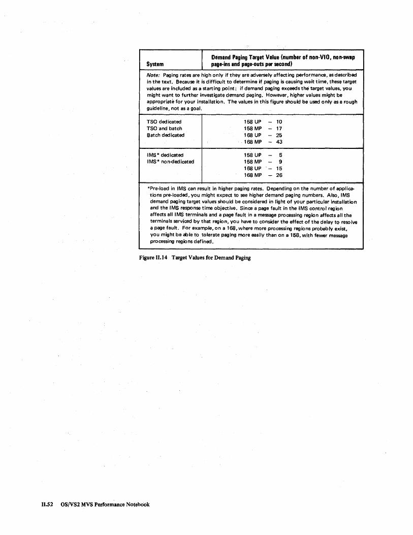
System Demand Paging Target Value (number of non-VIO, non-swap page-ins and page-outs per second)
Note: Paging rates are high only if they are adversely affecting performance, as described in the text. Because it is difficu·lt to determine if paging is causing wait time, these target values are included as a starting point: if demand paging exceeds the target values, you might want to further investigate demand paging. However, higher values might be appropriate for your installation. The values in this figure should be used Qnly as a rough guideline, not as a goal.
TSO ded icated 158 UP - 1Q TSOand batch 158 MP - 17 Batch dedicated 168 UP - 25
168 MP - 43
IIVlS* dedicated 158 UP - 5 IMS* non-<fedicated 158 MP - 9
168 UP - 15 168 MP - 26
*Pre-Ioad in IMS can result in higher paging rates. Depending on the number of applications pre-loaded, you might expect to see higher demand paging numbers. Also,IMS demand paging target values should be considered in light of your particular installation and the IMS response time objective. Since a page fault in the IMS control region affects all IMS terminals and a page fault in a message processing region affects all the terminals serviced by that region, you have to consider the effect of the delay tQ resolve a page fault. For example, on a 168, where more processing regions probably exist, you might be able to tolerate paging more easily than on a 158, with fewer message processing regions defined.
Figure 11.14 Target Values for Demand Paging
11.52 OS/VS2 MVS Performance Notebook

OS/VS2 MVS Performance Notebook
Part II
Bulletin 4.1.0 Swapping
Real Storage Analysis • swapping
March 1977
The RMF paging activity report lists the number of swaps according to the type of swap. Solutions to reduce swapping depend on the type of swap being experienced:
• input terminal wait swaps are "productive" swaps and, therefore, not usually of concern. They reflect the transaction rate and the only way to reduce their rate is to reduce the transaction rate - which is not usually desirable.
• output terminal wait swaps should be close to zero. They can occur for two reasons:
the TIOC does not have sufficient output buffers, because TSO commands or CLISTs are producing unusual amounts of output or because sufficient buffers were not allocated initially. The SRM treats this condition as the end of a transaction and automatically swaps out the address space until the output buffers are emptied. If swaps occur consistently for this reason, evaluate the OWAITHI value in the IKJPRMxx PARMLIB member.
application programs are issuing TPUT SVCs with the HOLD keyword. If this is true, re-examine the necess.ity of coding HOLD.
• requested swaps occur automatically when V=R or non-swappable jobs or steps are started. The only way to reduce these is to reduce the amount of nonswappable work, or work running V=R.
• auxiliary and real pageable storage shortage swaps should not normally occur and, if they do, can Signify a potentially serious problem. For auxiliary storage shortage swaps, first check the job swapped out (it is identified at the system console) for a VIO loop - VIO loops can cause excessive auxiliary page slots to be allocated. Otherwise, these types of swap indicate the need for additional hardware resources (auxiliary or real storage, depending on the type of swap), unless one of the following is possible:
- the workload can be reduced and/or critical address spaces (those that acquire auxiliary storage page slots or fIXed frames at the greatest rate) can be moved to non-critical shifts.
- more auxiliary storage can be assigned to the page data sets or fIXed requirements in real storage can be reduced to make more pageable storage available.
• long wait swaps usually occur as a result of the STIMER macro or enqueue contentiQn - in the first case, reduce use of STIMER; in the second, identify and reduce or eliminate the source of contention. Long wait swaps can also occur during MOUNT processing (waiting for a DASD volume to be mounted) and during allocation recovery (waiting for a reply to a WTOR).
Chapter 11.4: Investigating the Use of Real Storage 11.53

Real Storage. Analysis • swapping
Bulletin 4.1.0 Swapping (continued)
March 1977
• unilateral and exchange-on-recommendation~J)alue swaps are based on the IPS specification. Reducing these involves modifications to the IPS specification -see the Initialization and Tuning Guide.
• enqueue exchange swaps are reduced by identifying and reducing the source of contention.
• detected wait swaps occur when an address space in storage has been nondispatchable for a fixed period of time. Solutions depend on why the address space is nondispatchable; for example:
- an initiator runs out of work. Re-examine the number of initiators and the classes assigned to each.
the address space is enqueued on a resource in use by another address space. Identify and reduce or eliminate the source of contention.
11.54 OS!VS2 MVS Performance Notebook

OS/VS2 MVS Performance Notebook
Part II
Bulletin 4.2.0 Demand paging
Real Storage Analysis • demand paging
March 1977
High demand (non-VIO non-swap) paging indicates the possible over-commitment of real storage - that is, too many users competing for real storage. If sufficient frames are not available on the available frame queue to assign to users as they require more storage, pages are stolen (according to the unreferenced interval count) to free required frames. If the pages stolen are referenced again, they must be reclaimed (if they have not been paged out) or paged-in (demand paging).
Steps to Reduce Demand Paging
There are several steps that can be taken to reduce demand paging:
1. Increase the size of pageable storage by reducing the number of modules, data areas, and control blocks that are fixed.
2. In the pageable areas (PLPA and private), examine module packing and CSECT ordering to try to achieve efficient page reference patterns: in terms of density of reference (so that fewer pages are active at one time) and frequency of reference (so that pages that are stolen due to a high unreferenced interval count are not re-referenced).
3. Identify users with exceptionally large working sets and investigate workload changes to avoid the concurrent execution of these users.
4. Reduce the multiprogramming level.
Each of these steps is described in the following topics. To visualize how storage is being used and to help focus on specific areas, it is useful to draw a storage map of the system. The RMF paging activity report provides the number of frames assigned to the following areas:
• SQA (always fixed) • LPA/CSA - fixed • LPA/CSA - pageable • private area - fixed • private area - pageable • available (unused) frames • nucleus.
SIR can be used to break down the private area by user.
ChapterIl.4: Investigating the Use of Real Storage U.5S

Real Storage Analysis • demand paging
Bulletin 4.2.0 March 1977 Demand paging (continued)
Reducing Fixed Storage Requirements
The feasibility of and approach to reducing ftxed storage requirements depends on
the area that is fLXed:
• The nucleus can be reduced by generating fewer options - for example, do not specify ACR (alternate CPU recovery) if the system is not MP; remove excess unused UCB definitions.
• The SQA is difftcult to reduce. Identifying the users responsible for fLXed frames in SQA requires dumping the SQA and trying to trace who was responsible for the various entries in the system control blocks. It is not always feasible to reduce SQA, and because the effort to try is signiftcant, SQA is not a prime candidate for reduction.
• The amount of CSA ftxed depends on the environment. In batch or TSO environments, almost none of CSA is ftxed. In IMS environments, the amount ftxed depends on the IMS ftx options chosen by your installation and the size of the pools. Because IMS pools are fLXed to improve I/O performance and response time, reducing the amount fLXed in order to reduce demand paging involves trade-offs: you must assess the potential impact on I/O performance and response time of reducing fLXed CSA.
• To reduce ftxed LPA, examine the choice of modules in the ftx list (IEAFIXxx member of P ARM LIB) to determine if reentrant modules might better be placed in pageable LPA. If a module is frequently used, it will likely remain in storage, although it is placed in PLPA.
• In the private area, every address space will have a minimum set of ftxed frames - usually ftve or six - for LSQA. Focus on those address spaces whose ftxed areas greatly exceed this minimum set. (SIR reports the number of fLXed frames assigned to each address space.) Solutions to reducing the fLXed areas depend on the user and what is being ftxed.For example, TCAM often causes a large number of frames to be ftxed for buffers; these can be reduced by reducing the number and/or size of the buffers, although possible impact on I/O performance must also be considered - see the topic "TeAM" in Part III.
Page Reference Pattern of Pageable Modules
Paging can be decreased in PLP A and the private areas by efftcient page reference patterns. The goal is to localize page references in terms of the number of pages required at a time (density of reference) and in terms of time (frequency of reference, so that a page that might be stolen after disuse is not referenced again).
11.56 OS/VS2 MVS Performance Notebook
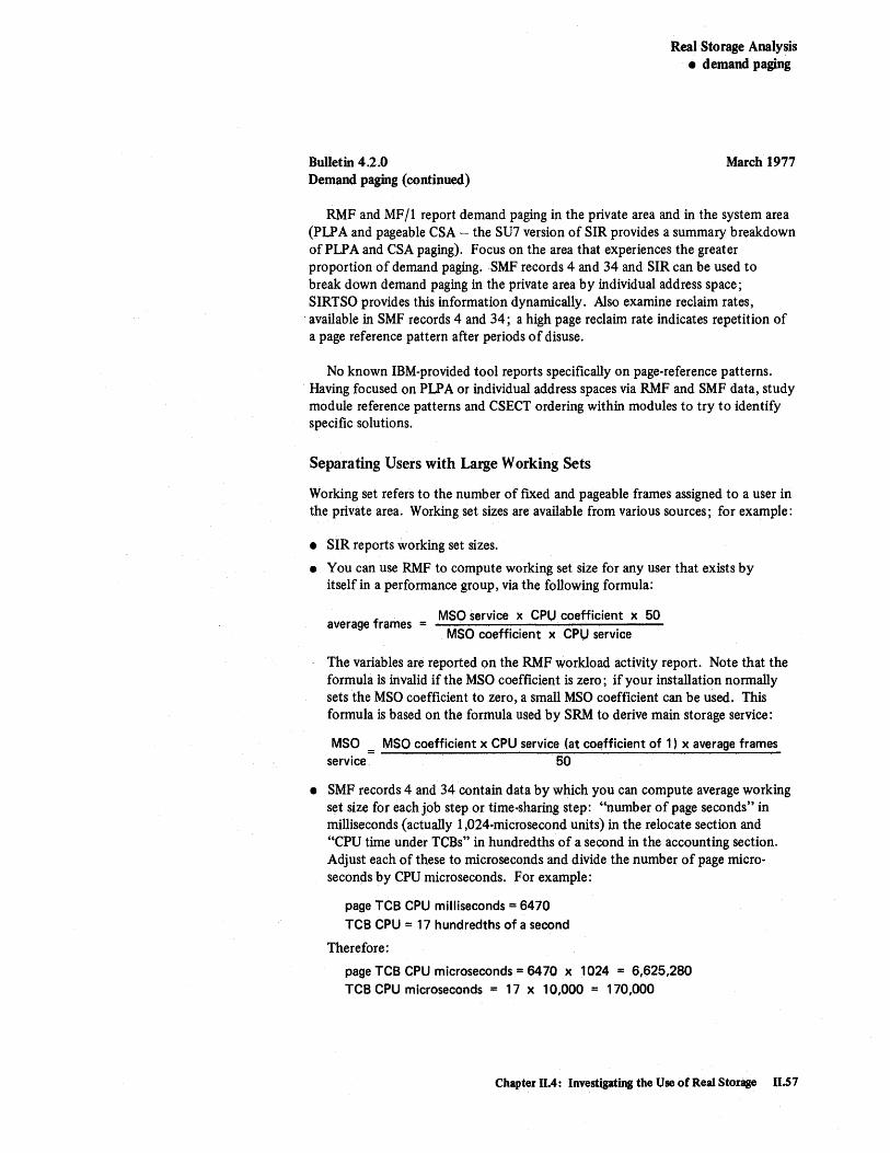
Bulletin 4.2.0 Demand paging (continued)
RealStorage Analysis • demand paging
March 1977
RMF and MF /1 report demand paging in the private area and in the system area (PLP A and pageable CSA - the SU7 version of SIR provides a summary breakdown of PLP A and CSA paging). Focus on the area that experiences the greater proportion of demand paging. SMF records 4 and 34 and SIR can be used to break down demand paging in the private area by individual address space; SIRTSO provides this information dynamically. Also examine reclaim rates, available in SMF records 4 and 34; a high page reclaim rate indicates repetition of a page reference pattern after periods of disuse.
No known IBM-provided tool reports specifically on page-reference patterns. Having focused on PLP A or individual address spaces via RMF and SMF data, study module reference patterns and CSECT ordering within modules to try to identify specific solutions.
Separating Users with Large Working Sets
Working set refers to the number of flXed and pageable frames aSSigned to a user in the private area. Working set sizes are available from various sources; for example:
• SIR reports working set sizes.
• You can use RMF to compute working set size for any user that exists by itself in a performance group, via the following formula:
f MSO service x CPU. coefficient x 50
average rames = MSO coefficient x CPU service
The variables are reported on the RMF workload activity report. Note that the formula is invalid if the MSO coefficient is zero; if your installation normally sets the MSO coefficient to zero, a small MSO coefficient can be used. This formula is based on the formula used by SRM to derive main storage service:
MSO = MSO coefficient x CPU service (at co~fficient of 1) x average frames ~~~ 00
• SMF records 4 and 34 contain data by which you can compute average working set size for each job step or time-sharing step: "number of page seconds" in milliseconds (actually 1 ,024-microsecond units) in the relocate section and "CPU time under TCBs" in hundredths of a second in the accounting section. Adjust each of these to microseconds and divide the number of page microseconds by CPU microseconds. For example:
page TCB CPU milliseconds = 6470
TCB CPU = 17 hundredths of a second
Therefore:
page TCB CPU microseconds = 6470 x 1024 = 6,625,280 TCB CPU microseconds:;: 17 x 10,000 = 170,000
Chapter 11.4: Invest.gating the Use of Real Storage 11.57

Real Storage Analysis • demand paging
Bulletin 4.2.0 March 1977 Demand paging (continued)
And:
k· . 6,625,280 38 97 ~ 39 average wor ·1 ng set SI ze = = . . ,..., pages 170,000
Focus on those users with exceptionally large working sets. If more than one batch job has a large working set, try to execute them separately; for example: assign the large jobs to a single domain with a maximum MPL of 1; or assign them to a unique job class and assign that job class to only one initiator. Ways to reduce working set size are reducing fIXed requirements in private address spaces and ensuring efficient page-reference patterns - as described in the previous topics.
Reducing the Multiprogramming Level
If no batch jobs have exceptionally large working sets, and reducing fIXed requirements and investigating page reference patterns do not result in sufficiently reducing demand paging, lower the multiprogramming level in the system. This can be done by lowering the MPL for specific domains, which allows you to control what work will have the lower MPL. On a system level, it is also possible to achieve a lower multiprogramming level by changing the threshold values for the page fault rate and the VIC (unreferenced interval count). However, unlike changing MPLs, this cannot be done via an external control (it requires zapping constants; see the Initialization and Tuning Guide for details on these constants). For additional information on changing the MPLs or zapping constants to achieve lower demand paging rates in IMS mixed environments, see the topic "Demand paging in IMS" in Part III.
11.58 OS/VS2 MVS Performance Notebook
OS/VS2 MVS Performance Notebook
Part II
Bulletin 4.3.0 VIO paging
Real Storage Analysis • VIO paging
March 1977
The first step in investigating high VIO paging rates is to review VIO usage to determine if it is being used effectively; see the Initialization and Tuning Guide for VIO performance considerations. (Additional hints on VIO usage will be added to Part III of this book in a future update.) IfVIO paging must be reduced, identify the data sets using VIO. Records 4 and 34 in SMF identify the VIO pageins on a user level. Focus on those users with a relatively high number of VIO page-ins and identify the VIO data sets being used by these users. Consider using normal allocation for the VIO data sets that experience a high VIO paging rate.
Chapter 11.4: Investigating the Use of Real Storage 11.59

11.60 OS/VS2 MVS Performance Notebook
Real Storage Analysis • reducing time to resolve page faults
OS/VS2 MVS Performance Notebook
Part II
Bulletin 4.4.0 Reducing the time to resolve page faults
March 1977
Several measurements have shown that performance is degraded if a page-in requires, on the average, more than approximately seventy milliseconds to resolve. The following formula can be used to determine the approximate amount of time required to resolve a page-in in your system:
RCVASMQA = average time per page-in
total system paging rate
where RCVASMQA (ASM queue length average) is provided by the RMF trace and total system paging rate is reported on the RMF paging activity report. (This formula can also be used to compute the average time to resolve a page-out.) The time computed via this formula is from when ASM receives a page request until I/O is complete and the requestor is posted. Note, however, that the requestor will not necessarily be dispatched immediately after being posted; the requestor's wait time, therefore, can be longer than the time to resolve the page-in.
If page-ins are taking excessive time to resolve, examine the number and placement of page, PLP A, and common data sets - see the Initialization and Tuning Guide for suggestions on the placement of paging data sets.
Chapter 11.4: Inve$tigating the Use'of Real Storaae 11.61

..
11.62 OS/VS2 MVS Performance Notebook

Chapter 11.5: User-oriented Performance Problem Analysis
User-oriented objectives include response time for interactive transactions and turnaround time for batch. Use the analysis described in this chapter to address the following problems:
• Response time is inadequate for a particular class of transactions (for example, TSO trivial transactions).
• Turnaround time is inadequate for a particular class of jobs.
• Turnaround time is inadequate for a specific application.
The analysis is aimed at answering, "Why is the work in question waiting (that is, not receiving the service it requires to meets its objective) ?"
Identifying Why Work is Being Delayed
The major difficulty in solving user-oriented performance problems is determining why the work in question is not receiving the service it requires to meet its performance objective. This requires measurements on an address-space level and often requires the use of GTF data or the trace table to trace and time events attributable to the work in question.
There are several major causes of delay:
• waiting to start or excessive input queue time.
• while in storage, waiting for the processor.
• excessive demand paging.
• waiting for I/O to complete (including delays due to operational bottlenecks).
• enqueue contention for TSO or batch work or, for IMS work, data base contention.
• excessive swapping (applicable to TSO and batch work only, since the IMS control region must be nonswappable and it is recommended that the IMS message processing regions be made nonswappable; however, excessive swapping ofTSO or batch work can affect IMS response time, due to system interference).
• contention for locks and IMS latches.
With the exception 0 f locks and latches, investigation 0 f each 0 f these is described in the bulletins at the end of this chapter. (Information on investigating lock/latch contention will be included in a future update.)
Chapter 11.5: User-oriented Performance Problem Analysis 11.63

There is no firm order in which to investigate the possible causes - if a specific resource is critical in your installation, investigate causes related to it first. For example, if storage is critical, start by checking swapping, excessive paging, and waiting to start. However, beware that you cannot always focus on one cause until others have been eliminated. For example, if the work is in storage and is not obtaining sufficient access to the processor, you cannot assume the work is being denied access to the processor unless you know it is not waiting due to I/O or enqueue conter.tion.
Once the causes of wait time are identified, initial solutions involve increasing access to the resources causing the delay via specifying preference of the work in question over other work in the system (that is, workload management). Means of doing this include dispatching priority, the IPS performance 'objective, and, for batch/IMS, the number and structure of initiators/message processing regions, respectively. Use of such controls implies trade-offs for other work in the system. If such trade-offs cannot be tolerated, the direction of the analysis must shift to optimizing use of the resource(s) in question - or prioritizing the objectives for different types of work, modifying objectives, or considering additional hardware. Investigating the use of the major system resources - processor, I/O resources, and real storage - is described in Chapters 11.2, 11.3, and 11.4, respectively. For example, if the processor is critical and increasing the DPRTY of the work in question will have an unacceptable effect on other work, you can examine the use of processor time to eliminate or reduce non-productive processor time - see Chapter 11.2, "Investigating the Use of Processor Time."
Solutions to different causes.of delays can also be conflicting. For example, assume a TSO trivial response time problem is being investigated and two causes of wait time are identified: excessive paging and waiting to start. After investigating possible solutions to each of these problems, you focus on reducing the multiprogramming level of the system to reduce paging and increasing the maximum multiprogramming level for TSO trivial transactions to reduce their wait-to-start time. Other work in the system will have to be reduced to achieve the lower system workload level and the higher TSO workload level, which can impact meeting the performance objectives of the other work. (A possible benefit, however, is increased productive processor time due to decreased paging, which might offset lower multiprogramming levels by decreasing t0tal elapsed time.) Again, at this point, you might have to examine the use of the critical resource (in this case, real storage) or consider modifying the objectives or obtaining additional hardware.
Possible solutions to each of the causes of wait time are included in the bulletins at the end of this chapter.
11.64 OS/VS2 MVS Performance Notebook
OS/VS2 MVS Performance Notebook
Part II
Bulletin S .1.0 Waiting to start
User-oriented Problem Analysis • waiting to start
March 1977
Possible Problem: work in question is waiting to start. Investigation of and possible solutions to this problem depend on the type of work: batch, IMS, or TSO, as described below.
Batch
Investigating Problem: Wait-to-start time is available in SMF record 5: the time the initiator selected the job (offset + X'27') less the time the reader recognized the
. JOB card (offset + X'16'). Determining if the wait-to-start time is excessive requires a judgment based on the amount of time the job spends executing and the objective for the job - or based on the average wait-to-start time experienced when jobs are receiving satisfactory turnaround time.
Possible Solutions: Re-evaluate the number of initiators and the job classes aSSigned to each initiator. Also examine the external scheduling criteria for the jobs and their grouping into job classes: for example, can some of the jobs be moved to a separate class and that class executed during an off-shift? Check for jobs that violate job class standards.
IMS Investigating Problem: Input queue times for IMS transactions (equivalent to wait-to-start time for TSO/batch work) are reported by the IMS/VS log transaction analysis utility program. (See the IMS/VS Utilities Reference Manual for details on this program.) To judge if input queue times are high, compare them to average input queue times observed when performance objectives are being met. Note that the computation of input queue time (from information on the IMS log) does not include possible delays at the terminal or on the terminal line.
Possible Solutions: Several factors can contribute to IMS transactions being delayed on the input queue:
• The IMS control region cannot schedule the transaction to an MPR. This can occur because:
- All MPRs are active. Re-examine the number of MPRs, the classes served by each, and the scheduling priority of the transaction type being delayed (as specified in the PRTY parameter coded on the TRANSACT macro for this transaction type: lower the limit count if the limit priority is not being used; or raise the limit priority if it is being used).
- The control region cannot allocate space for the required control blocks (a non-zero return code is returned from the block-builder), due to insufficient virtual storage assigned to work pools (PSB, PSBW, DMB, and/or DBWP). Re-examine the size of the work pools.
Chapter 11.5: User-oriented Performance Problem Analysis 11.65

User-oriented Problem Analysis • waiting to start
Bulletin 5.1.0 March 1977 Waiting to start (continued)
• If insufficient message queue buffers are available to handle the arrival rate of transactions, they will be sent to the message queue data set (OSAM), whether or not an MPR is available to process them. This will delay the transaction by at least the I/O time to and from the message queue data set.
TSO
Investigating Problem: Examine GTF SRM trace data for the average time from user-ready to restore-complete SYSEVENTs. If this time exceeds approximately one-half second, TSO transactions are being kept out of storage. For TSO trivial transactions, where swapping usually occurs only once per transaction, wait-tostart time can also be computed from data available on the RMF workload activity report:
avg. transaction service rate ---------- X avg. time of ended transaction = residency time avg. absorption service rate
and:
avg. time of ended transaction - residency time = wait-to-start time
Possible Solutions: The delay can occur for one of two reasons:
• the swap-in is taking too long (examine the time from swap-in-start to restorecomplete SYSEVENTs in the GTF SRM trace data). Poor swap performance is usually best addressed by the number and placement of page and swap data sets - see the Initialization and Tuning Guide for suggestions.
• swap-in is being delayed (examine the time from user-ready to swap-in-start SYSEVENTs in the GTF SRM trace data). This can occur because: (1) the target MPL, maximum MPL, or domain weight for this domain is low compared to the average number of users; or (2) non-trivial transactions execute in the same domain as trivial transactions and are not pre-empted when new transactions become ready. (Note, however, that pre-emption can result in an excessive swap-to-transaction ratio. It is best to place trivial and non-trivial transactions in separate domains, as described below.)
In the first case, adjust the MPLs and the weight for the domain. Beware, however, that this can adversely affect other work in the system. The target MPL might be low because of broader performance problems: for example, processor or real storage constraints. If true, it is necessary to identify the critical resource and examine its use. The description of step 4 in Chapter ILl describes how to focus on the major resources (system-oriented performance analysis); chapters 11.2, 11.3, and 11.4 describe investigating the use of processor time, VO resources, and real storage, respectively.
U.66 OS/VS2 MVS Performance Notebook

Bulletin 5.1.0 Waiting to start (continued)
User-oriented Problem Analysis • waiting to start
March 1977
In the second case, the preferred solution is to place trivial and non-trivial transactions in separate domains - associate the second period of the TSO performance group with a different domain than the first period. If the two periods already specify different domains, re-examine the duration of the first period (as specified by the DUR parameter); it might be too long, allowing nontrivial transactions to execute in the first period.
If the periods of the TSO performance group are associated with the same domain, an alternate solution is to ensure that transactions that enter the second period are pre-empted by transactions that become ready. To accomplish this, define the IPS performance objective such that, at zero service level, transactions in the second period are at a lower workload level (more than one lower) than transactions in the first period. On a graph, the objectives for periods 1 and 2 should look as follows, to ensure pre-emption of transactions in period 2:
Service Units
1,000
100 Workload Level
Pre-emption of transactions in period 2 will not occur if the IPS performance objective results in a graph such as the following:
Service Units
1,000
100 Wo rkload Level
For details on defining IPS performance objectives, see the Initialization and Tuning Guide. Warning: Associating periods of the TSO performance objective with the same domain and using the IPS performance objective to ensure preemption can, however, result in an excessive swap-to-transaction ratio. Beware of the possible adverse effects of this solution, especially if real storage is a critical resource at your installation.
Chapter 11.5: User-oriented Perfonnance Problem Analysis 11.67

11.68 OS/VS2 MVS Performance Notebook

OS/VS2 MVS Performance Notebook
Part II
Bulletin 5.2.0 Access to the processor
User-oriented Problem Analysis • access to the processor
March 1977
Possible Problem: While in storage, the work in question cannot gain sufficient access to the processor.
Investigating Problem: Compare the residency time of the work in question to the amount of processor time used. For TSO and batch work, residency time and TCB processor time are available in SMF records 5 for batch jobs and records 35 for TSO transactions. For [MS, residency time is the time a transaction is active in an MPR; it is reported as "time processing" in the detailed transaction report produced by the IMS/VS log transaction analysis utility program. The average TCB processor time per message is reported on the application accounting report produced by the IMS/VS statistical analysis utility program.
Judgment of the processor-to-residency-time ratio should be based on several factors: whether the work is swappable or non-swappable; the amount of processor time required by the work in question; the objective of the work in question. It is best to judge the processor-to-residency-time ratio in light of the ratio usually observed when performance objectives are being met. As a starting point for swappable TSO or batch work, you might expect to see a ratio of approximately 1 :5.
Note that, if you decide the work is not experiencing an adequate processorto-residency-time ratio, you cannot immediately assume that the work is being denied aCcess to the processor. You must also consider the possibility that it is waiting due to I/O or enqueue contention - see bulletins 5.4.0 and 5.5.0, respectively.
SIR can be used to identify those address spaces of higher dispatching priority that are using large amounts of processor time - in increasing the work-inquestion's access to the processor, you will want to consider trade-offs with these address spaces.
Chapter 11.5: User-oriented Performance Problem Analysis 11.69
User-oriented Problem Analysis • access to the processor
Bulletin 5.2.0 March 1977 Access to the processor (continued)
Possible Solutions: Increase the DPRTY of the work in question. (Note, however, that this will affect other work in th~ system.) For example, in a system containing a DB/DC application and heavy JES activity (RJE, local printers, and so on), JES will require significant amounts of processor time; as a default, JES will execute at a higher dispatching priority than the DB/DC application, therefore impacting the application's access to the processor. Placing the application at a higher DPRTY than JES will improve its performance.
If the work in question is in the APG mean-time-to-wait group, you can place a specific job above the mean-time-to-wait group to improve its access to the processor; or use the rotate priority for a group of jobs with heavy processor demands.
11.70 OS!VS2 MVS Performance Notebook
OS/VS2 MVS Performance Notebook
Part II
Bulletin 5.3.0 Excessive demand paging
User-oriented Problem Analysis • excessive demand paging
March 1977
Possible Problem: Work in question is being delayed due to excessive demand (non-VIO non-swap) paging.
Investigating Problem: In investigating if excessive demand paging is delaying the work in question, you first want to establish if the system in general is experiencing excessive paging, regardless of whether the work in question has a high paging rate. High demand paging can affect throughput, which affects the performance of all work in the system, including the work in question. Paging also "costs" in terms of processor time, which again can affect the work in question. The problem is judging if a paging rate is "high" - paging rates vary widely and your system can have a high rate, as compared to other installations, and good performance. Paging rates are high only if they are adversely affecting performance (such as costing excessive processor time). Chapter 11.4 describes the ways in which excessive paging affects performance; figure 11.14 gives target values for demand paging, to use as a starting point if your installation is not sure how much demand paging is acceptable in your system. If demand paging in your system seems high, it should be investigated - see Bulletin 4.2.0 in chapter 11.4. For IMS systems, see also the topic "Demand paging in IMS" in Part III.
You can also investigate paging rates as an indication of an application's misuse of its own address space. Information on paging on an address space/job level is available after the fact via SMF and SIRBATCH, and dynamically via SIRTSO. (Note that, for IMS, paging rates are reported for MPRs and the control region; no paging statistics are available for individual IMS applications. For IMS tuning, however, CSA paging is the most important paging factor to investigate - not paging by individual applications.)
Two numbers are of interest when investigating the potential problem of excessive paging for specific batch applications: page reclaims and demand pageins (non-VIO, non-swap page-ins). These numbers are available on a job step level in SMF type 4 records and on a job level in SIR.
The number of page reclaims can indicate an application's mis-use of its own address space, if it is high compared to the number of reclaims experienced by other address spaces. (Note, however, that a high reclaim rate is not of as great a concern as high demand paging rates, because of the relatively lost "cost" of reclaims.)
Chapter 11.5: User-oriented Performance Problem Analysis 11.71

User-oriented Problem Analysis • excessive demand paging
Bulletin 5.3.0 March 1977 Excessive demand paging (continued)
A rule-of-thumb for judging the number of demand page-ins is that, at a minimum, the amount of processor time used by the job between demand page-ins should at least equal to [he time taken to resolve a page-in. To compute the average processor time between demand page-ins, divide the total processor time (from SMF record 5) by the number of demand page-ins and compare this to the average time required to resolve a page-in. The average time required to process a page-in can be computed as RCVASMQA (ASM queue length average from the RMF trace) divided by the total system paging rate. (Note that excessive time to satisfy a page transfer, as computed by this formula, can also contribute to delays of the work in question -see bulletin 4.4.0 in chapter 11.4.) The application is experiencing excessive paging if the average processor time between demand page-ins is less than the time required to resolve a page-in. A less exact test of excessive demand page-ins is a simple comparison of the application's demand page-in rate to that of other address spaces in the system.
SMF and the srn version of SIR also provide data on whether page faults occurring in an address space are in its own address space or in PIP A/CSAwhich information might be needed for determining a solution to the performance problem.
Possible Solutions: If investigation of a particular application revealed excessive paging for that application in particular, solutions pertain to the application's use of its own address space - for example, repetition of a page reference pattern after periods of disuse. Study the program's CSECT ordering and module reference patterns to identify specific solutions.
11.72 OS/VS2 MVS Performance Notebook

OSjVS2 MVS Performance Notebook
Part II
Bulletin 5.4.0 Waiting for I/O
User-oriented Problem Analysis • waiting for I/O
March 1977
Possible Problem: work in question is waiting for I/O to complete. Investig~tion of this potential problem varies for TSO or batch work and IMS work.
TSO or Batch
Investigating Problem: Correcting imbalances in channel and device activity on a system level will not necessarily correct I/O delays encountered by the work in question. You must investigate the specific I/O resources being used: SMF records type 4 (batch) and 34 (TSO) identify the devices assigned to non-spooled data sets and the channels used for those devices.
Possible Solutions: Solutions to I/O delays depend on the bottleneck contributing to the delay - for example, operational bottlenecks due to volume mounting; excessive SEEK time due to poor data set placement; and so on. Chapter 11.3, "Investigating the Use of I/O Resources," describes bottlenecks that contribute to I/O delays, ways to determine if they are occurring, and suggestions for reducing them. Chapter 1.3, "Pre-initialization MVS Performance Factors," describes possible operational bottlenecks.
IMS
Investigating Problem: To investigate the possibility of I/O delays, start by looking at RMF or MF /1 channel and device reports for evidence of delay on the volumes of the data base used by the work in question. For example, examine queue length measurements and the average time to service a request on the device(s) accessed -see bulletin 3.1.0 in Chapter 11.3 for descriptions of these measurements. Bulletin 3.2.0 in Chapter 11.3 describes measurements that might indicate specific bottlenecks in the path to the device. In addition, long IW AIT times in the DC Monitor reports might indicate possible I/O contention.
Possible Solutions: If I/O delays can be attributed to contention for the device on which the data base resides, examine the placement of the data base on devices: consider spreading the data base across more devices; and/or ensure the placement of highly-used parts of the data base on different paths. I/O resource contention can also be reduced by reducing the number of EXCPs/SIOs - see bulletin 3.4.0 in Chapter 11.3.
ChaJ)ter 11.5: User-oriented Performance Problem Analysis 11.73

11.74 OS/VS2 MVS Performance Notebook
OSjVS2 MVS Performance Notebook
Part II
Bulletin 5.S.0 Enqueue/data base contention
User-oriented Problem Analysis • enqueue/data base contention
March 1977
Possible Problem: Work in question is delayed due to enqueue contention (TSO or batch work) or data base segment contention (IMS work).
TSO or Batch
Investigating Problem: The occurrence of enqueue exchange, long wait, and detected wait swaps (reported in swap-out counts on the RMF paging activity report) can indicate the presence of enqueue contention on a system level. On an address-space level, SIRBATCH identifies address spaces that are waiting for a resource, the address space holding the resource, and the name of the resource.
Possible Solutions: The solution depends on the specific resource in contention and the address spaces vying for the resource. Some general suggestions to consider include the following:
• Use the JCL parameter FREE=CLOSE to ensure that resources are released when no longer needed.
• Assign the same job class to jobs that require the same resources and assign that job class to a single initiator.
• If a specific job monopolizes resources needed by other work in the system, run that job off-shift or limit the duration of its effect on other work by giving it a preferred dispatching priority and IPS performance objective to "hurry" it through the system.
• Structure the catalogs to reduce catalog contention.
IMS
Investigating Problem: The IMS/VS program isolation trace report utility program lists all transactions that had to wait while trying to enqueue on a data base record. The report includes the transaction waiting for the data base record, the transaction holding the record, and, if the /TRACE ALL option is specified, the elapsed time of the wait.
Possible Solutions: Program isolation in IMS reduces data base contention by allowing enqueues on particular segments and by resolving deadlock situations. Therefore, solutions to contention for data base records lie primarily in the area of workload management; for example, scheduling transactions that require the same data base records to a single MPR.
Chapter 11.5: User-oriented Performance Problem Analysjs 11.75

11.76 OS/VS2 MVS Performance Notebook

User-oriented Problem Analysis • excessive swapping
OSjVS2 MVS Performance Notebook
Part II
Bulletin 5.6.0 Excessive swapping
March 1977
Possible Problem: work in question is being delayed because .of swapping.
Investigating Problem: Swapping can delay work in two ways:
(1) The work is swapped too frequently.
(2) Once swapped out, the work waits too long before being swapped back in.
(1) In the first case, examine the swapping rates of the work in question. Swapping rates on a performance group level are available on the RMF workload activity report. The number of swaps per address space is available via SIRBATCH or SMF (record type 4 for batch; type 34 for TSO).
For TSO, a general target is a swap-per-transaction ratio of I.l:I; for trivial TSO, 1.0: 1. For batch, the acceptable number of swaps per job is installationdependent; in judging the number of swaps, consider factors such as the priority of batch work and the cost of swapping in terms of processor time. One rule-of-thumb is that swapping is not excessive for batch if batch swaps occur no more frequently than once every twenty seconds on a 158, once every eight seconds on a 168 (which translates to approximately 1% of processor time for batch swapping).
If you judge the swapping rate of the work in question to be high, determine why the swaps are occurring. SIRBATCH includes swap reason codes in report 3, the snapshots of jobs. You can also use a GTF SRM trace to trace the swaps experienced by the work in question. (Although swap-out counts by type of swap are provided on the RMF paging activity report, they are not broken down by address space.)
(2) In the second case (work in question is being delayed before being swapped back in), the average time in storage per swap should be at least equal to the amount of time out of storage per swap:
time in storage per swap ~ time out of storage per swap
Time in storage is residency time, reported in SMF record type 5 for batch, type 35 for TSO. Time out of storage is transaction active time (also from SMF records 5/35) less residency time.
Chapter 11.5: User-oriented Performance Problem Analysis 11.11
User-oriented Problem Analysis • excessive swapping
Bulletin 5.6.0 March 1977 Excessive swapping (continued)
The amount of time out-of-storage can be further broken down by computing the actual time required to perform the swap, versus time spent on auxiliary storage. Via a GTF SRM trace, compute the time from quiesce-start to swapcomplete SYSEVENTs (swap-outs) and from swap-in-start to restore-complete SYSEVENTs (swap-ins) for swaps of the work in question; and take their average.
Possible Solutions: The solution to minimizing swaps depends on the type of swap being experienced. See Bulletin 4.1.0 in Chapter 11.4.
If work is being delayed before being swapped back in, the solution might also depend on the type of swap - for example, on a long or detected wait swap, the delay might be caused because the address space is enqueued on a resource in use by another address space. The delay can also be caused by an inappropriate definition of the IPS performance objective for the work in question (for example, improper domain weights). For information on these factors~ see the Initialization and Tuning Guide.
Some applications (such as DB/DC applications) should be executed as nonswappable. For IMS, it is recommended thatthe message processing regions be made nonswappable. (It is a reqUirement that the IMS control region be made nonswappable.) -
11.78 OS/VS2 MVS Performance Notebook
Blocksize and buffer hints
Channel balancing
Configuration • rules-of-thumb • miscellaneous hints
Demand paging in IMS
Dispatching priority hints
Domain controls
JES2 hints
Seek time, reducing
Shared DASD hints
SVC hints
TCAM hints
VSAM catalog hints
PART In: Performance Hints
Part III: Performance Hints 111.1

111.2 OS/VS2 MVS Performance Notebook
OS/VS2 MVS Performance Notebook
Part III
Blocksize and Buffer Hints
Blocksize and Buffers
March 1977
Increasing the SAM buffer pool size via BLKSIZE and/or BUFNO will help reduce EXCP rates. The EXCP/IOS path length in MVS has increased substantially from MVT. The number oftimes this code is executed,however, can be reduced either by increasing blocksizes or by chaining requests together. Since chained scheduling (OPTCD=C) is now the default in most cases, increasing the number of buffers usually increases the number of requests that are chained together.
Although there is a trade off of storage for processor cycles with this suggestion, large buffer pools in MVS no longer occupy a major part of the potential user region. Since an individual buffer is ftxed only while I/O is being performed to it, the system can automatically adjust real storage requirements based on the actual data rate. However, large buffer pools in an I/O-limited process can lead to large real storage requirements and long periods of channel monopolization.
Use an analysis of SMF records 14/15 to focus on data sets that have high EXCP counts. Consider the following:
Unit Record Devices: QSAM is preferable to BSAM for all options. For output, use control characters rather than the CNTRL macro. For printers, specify OPTCD=C and do not use PRTOV: they are incompatible.
Tape: Use QSAM unless NOTE/POINT or BSP is needed. With QSAM (or a userprovided I/O overlap) avoid RECFM=U and choose a multiple of 4096 for BLKSIZE. For QSAM programs that are limited by tape I/O speeds, you can assume that half of the buffer pool is ftxed at a time, and that the channel is locked long enough to transmit the corresponding amount of data.
DASD: Allocate data sets by cylinders and use full or half-track blocking if most processing is sequential. Allocating data sets by cylinders reduces overhead associated with testing if end-of-extent has been reached, since the test is only performed at the end of each cylinder rather than at the end of each track.
Where possible, use QSAM rather than BSAM to provide full automatic I/O over· lap and complete BLKSIZE/BUFNO flexibility. Increasing BSAM NCP will have no effect unless the application program provides I/O overlap and can adjust to an increased number of outstanding requests. Increasing QSAM BUFNO can reduce both EXCP/IOS time and total elapsed time to a fraction of their former value.
Part III: Performance Hints .111.3

Blocksize and Buffers
Blocksize and Buffer Hints (continued) March 1977
Avoid track overflow or undefined length records (RECFM=U or T). To reduce channel busy time, use RECFM=FBS when creating physical sequential data sets. With FBS, the incorrect-length flag in the Read Data CCW indicates the last block in the data set. Therefore, an EXCP need not be issued to read the EOF mark. RECFM= FBS cannot be used where short blocks might be imbedded within the data.
You can achieve minimum EXCP overhead by setting BUFNO (or NCP) to twice the number of blocks per allocation unit (track or cylinder). Note, however, that this large a specification is not usually practical. With cylinder allocation and an application that is DASD limited, this approach will lead to channel lockouts, including block multiplexor channels, of up to 1/2 second. It will also force concurrent page fixes for up,to 60 pages, and as much as 2K of SQA per data set. The high real frame requiremens combined with the channel lockout could seriously degrade the system if the same channel is used for paging.'
Procedure libraries: Determine the size (the number of 80-byte records) of each procedure in the procedure library. Choose a blocksize that will allow a high percentage (85 - 90%) of the procedures to be totally read into storage in one EXCP. A 4K minimum blocksize is suggested. If reading data of few record members, override the chained-scheduling default.
Program Libraries: Program libraries should be examined for modules that are link-edited with the 'DC' attribute. If the load modules are frequently used, link-edit them again to remove the 'DC' attribute. This will minimize the processor time required to fetch those modules by reducing PCI handling. (Note, however, that this might result in an increase in elapsed time, due to missed connections, if there are multiple RLDs per text block.) PCls can also be reduced by increasing program libraries to full track blocking. The linkage editor has specific requirements when building the libraries at full track. See OSjVS Linkage Editor and Loader.
111.4 OS!VS2 MVS Performance Notebook

OS/VS2 MVS Performance Notebook
Part III
Channel Balancing
Channel Balancing
March 1977
Optional Channel Paths: The current implementation of the channel scheduler for MVS does not provide for rotation of the physical channel paths within logical channels. Thus, if the OPTCHAN keyword is specified on the 10DEVICE macro, making optional channel paths ava:ilable to devices, I/O will always be started on the primary path first (the logical channel with the lower channel number). Only if the primary channel path is busy will I/O be tried on the secondary channel path (the higher channel number). The logical channel with the lower channel number in an optional channel pair will thus tend to be busy more often. Although this does not significantly impact the performance of tape of non-RPS DASD devices, it does affect RPS DASD. The RPS operation must reconnect with the channel that started the operation; the imbalance of channel activity, however, increases the probability that it will not be able to reconnect.
You can increase the balance between optional and primary channels by the way in which you configure I/O resources. When devices that have only one I/O path are placed on a channel for which the OPTCHAN option is specified (that is, a channel which is one 0 f several paths to another device), configure them on the logical channel with the higher channel number. This helps achieve balance since the lower channel will probably be overloaded. However, if channels are selector channels, or if devices are in BURST mode (for example, tape), which makes multiplexor channels appear as selector channels, then devices should be placed on the logical channel with the lower channel number instead. This is because the lower channel gets driven first. By the time the logical channel with the higher channel number gets driven, that channel might be busy. It is best, for selectormode devices, to avoid configurations that have multiple logical channels sharing a common physical channel.
Part III: Performance Hints II1.S

111.6 OS/Vsi MVS Performance Notebook

OSjVS2 MVS Performance Notebook
Part III
Configuration Rules-of-Thumb
Configuration •. rules-of-thumb
March 1977
This topic presents some guidelines for judging the reasonableness of the MVS hardware configuration. The recommendations for the basic hardware resources are "rules-of-thumb" for judging the adequacy of your configuration; the formulas do not take into account tuning options and workload balancing. The likelihood of meeting performance objectives with current hardware resources depends on how well tuned the prior system was, flexibility in workload balancing, the size of the discrepancy between what is recommended and the actual resource (if a discrepancy exists), and similar factors. Although these guidelines, therefore, do not provide a firm answer to the question of adequate resources, they are useful as foresight for sizing the tuning effort and for predicting the likelihood of success with current hardware.
Processor
Processor utilization in MVS might be higher than in previous systems, primarily because of two factors:
• Reduced contention for serially usable resources in MVS (such as allocation resource serialization, fixed regions of real storage, and certain system data sets). This reduces processor wait time.
• Increased supervisor path lengths to support the additional function provided by MVS. Depending on the usage of various supervisor functions by a given workload, this might or might not cause an increase in processor time required to service that workload.
Consider the following guidelines when converting from MVT or SVS or from two MVS uniprocessors to an MP:
MVT: If converting to MVS from MVT, processor upgrade might be indicated if EXCP rates on the MVT system exceeded 100 per second on a 158, or 300 per second on a 168, and the major I/O files used by the workload cannot be reblocked to reduce the number of EXCPs required to read the same amount of data. Processor utilization in MVS can be estimated for most MVT environments with the following formula, based on hardware monitor measurements:
MVS processor~MVT problem state + (2 x MVT supervisor state)
Part III: Performance Hints III.7
Configuration • rules-of-thumb
Configuration Rules-of-Thumb (continued) March 1977
SVS: Several measurements have shown SVS and MVS processor utilization to be approximately the same to support similar workloads, but no measurements have been made in heavy I/O environments.
MVS UPs to MP: The processor is potentially a critical resource when converting from two MVS uniprocessors to an MP environment if total average utilization from both MVS UPs is greater than approximately 160% (as measured by MF/1, RMF, or a hardware monitor).
I/O Resources
Existing I/O resource configurations (channels, control units, and devices) should be, at the least, maintained on the MVS system. MVS systems frequently experience increased channel utilization compared to MVT and SVS. If the utilization of channels to eXisting RPS devices exceeds approximately 35% (measured by OSPT1 or a hardware monitor) on the pre-MVS system and response-oriented applications are to be supported on the MVS system, consider additional block multiplexor channels and control units for the MVS system. I/O resources should also be upgraded if growth or new applications are planned.
Real Storage
The rules-of-thumb in figure 111.1 can be used to roughly estimate the amount of real storage required for MVS; figure 111.2 is a worksheet for your estimates.
111.8 OS!VS2 MVS Performance Notebook
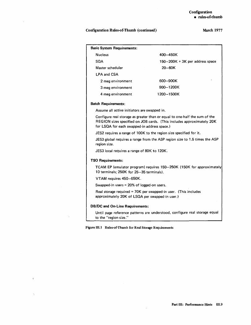
Configuration • rules-of-thumb
Configuration Rules-of-Thumb (continued) March 1977
Basic System Requirements:
Nucleus 400-450K
SOA
Master scheduler
150-200K + 3K per address space
20-60K
LPA and CSA
2 meg environment
3 meg environment
4 meg environment
Batch Requirements:
600-900K
900-1200K
1200-1500K
Assume all active initiators are swapped in.
Configure real storage as greater than or equal to one-half the sum of the REGION sizes specified on JOB cards. (This includes approximately 20K for LSOA for each swapped-in address space.)
JES2 requires a range of lOOK to the region size specified for it.
JES3 global requires a range from the ASP region size to 1.5 times the ASP region size.
JES3 local requires a range of 80K to 120K.
TSO Requirements:
TCAM EP (emulator program) requires 150-250K (150K for approximately 10 terminals; 250K for 25-35 terminals).
VTAM requires 450-650K.
Swapped-in users = 20% of logged-on users.
Real storage required = 70K per swapped-in user. (This includes approximately 20K of LSOA per swapped-in user.)
DB/DC and On-Line Requirements:
Until page reference patterns are understood, configure real storage equal to the "region slze. i
,
Figure 111.1 Rules-of-Thumb for Real Storage Requirements
Part III: Performance Hints 1II.9

Configuration • rules-of-thumb
Configuration Rules-of-Thumb (continued) March 1977
Installation __________________ Date ____ _
System Profile
Processor _____ TSO Active: Avg __ _ Batch Init
Storage ____ _ Max __ _ DB/DC __ _
Nucleus ___ K
SQA
Base _____ _
3K X No. address spaces ____ _
Master Scheduler
LPA + CSA
JES2
TCAM
TSO ( in)
BATCH ( in)
DB/DC
Available
Total K
Figure 111.2 Worksheet for Estimating Real Storage Requirements
111.10 OS/VS2 MVS Performance Notebook

OSjVS2 MVS Performance Notebook
Part III
Configuration Hints
Configuration • miscellaneous hints
March 1977
The following are miscellaneous hints on MVS hardware configurations. See also the preceding topic, rules-of-thumb for hardware configurations.
3270s and Tapes: Do not place local 3270s on the same selector or block multiplexor channel as tapes. Tapes should not be attached to a block multiplexor channel at all unless they are the only online device type on the channel, since they tie up the channel for the entire I/O operation. lOS will not service 3270 attention interrupts as long as tape I/O operations are active on the channel and additional requests are queued to be started when the current operation completes. Therefore, placing local 3270s and tapes on the same channel results in long response time delays for the 3270.
2305 vs. Additional Real Storage: If excessive swapping and demand paging are degrading performance in your system, consider the following:
• Adding a megabyte of real storage to reduce the amount of swapping and paging necessary seems to help batch environments of three megabytes or less.
• Adding a 2305 device to increase the speed of swapping and paging activity seems to help larger systems or systems with high TSO activity. (No amount of real storage will reduce the once-in/once-out swapping activity of TSO users for each transaction. However, additional real storage can result in fewer pages actually being transferred to auxiliary storage: more pages will be reclaimed.)
Part III: Performance Hints 111.11

111.12 OS/VS2 MVS Performance Notebook
OS/VS2 MVS Performance Notebook
Part III
Demand Paging In IMS
Demand Paging In IMS
March 1977
Changes to the SRM in SU7 can result in higher demand paging rates for IMS, which can in turn impact IMS response times in IMS-mixed environments. The following paragraphs highlight SU7 changes that affect demand paging and suggest ways to prevent excessive IMS paging in IMS-mixed environments. This write-up assumes knowledge of the SU7 SRM, including the indicators SRM uses to judge system contention, the page-stealing algorithm, and the concept of domains and MPLs.
There are two basic changes in the design of SRM that are significant to IMS paging:
• Address spaces are not swapped out to resolve storage constraints until the indicators of system contention are exceeded. Until the indicators are exceeded, storage shortages are resolved by demand stealing on a system-wide basis. As a result, the SU7 SRM might allow an environment to exist that is too storageconstrained for good online response times because its thresholds for recognizing system contention might be too severe for an online system.
• To determine which frames are eligible for stealing, the page-stealing algorithm adjusts every frame's unreferenced interval count (UIC) based on whether the frame was referenced in the preceding interval. Unlike the former SRM, there is no updating based on an address space's processor time, or any difference between swappable and non-swappable address spaces or between private and common areas. As a result, the frames likely to be stolen in systems with SU7 installed might be different from prior systems: address spaces that were insulated from stealing in pre-SU7 systems - such as IMS - can suffer more severe stealing; areas ofCSA and LPA with infrequent reference patterns -such as areas used by IMS - are no longer protected by the common bound algorithm.
There are two approaches to keep IMS from suffering excessive paging in systems with SU7 installed:
(1) by controlling other work in the system so that IMS receives sufficient resources.
(2) by changing the thresholds (the "happy values") by which SRM recognizes system contention and responds by lowering the multiprogramming level in the system.
Each of these approaches is described in more detail below.
Part III: Performance Hints III.l3
Demand Paging In IMS
\
Demand Paging In IMS (continued) March 1977
Controlling non-IMS Work
If the SU7 SRM allows processor or storage utilization to be too high for IMS, you can limit the amount of work ir the system by setting an appropriate maximum MPL for the TSO or batch domains - in the IPS or dynamically via the SET DOMAIN operator command. For batch, you might be able to achieve the same result simply by limiting the number of initiators. This should be effective if the batch workload is stable and can be controlled via installation scheduling - that is, if the amount of storage or processor time consumed by batch is directly related to the batch multiprogramming level.
Modifying the "Happy Values"
You might investigate changing (viasuperzap) the "happy values" for the indicators by which SRM recognizes system contention: processor utilization, ASM queue length, paging rate, or highestUIC in the system. Consider the following implications of comparing UIC count and ASM queue length "happy values" in IMS/batch versus TSO/batch systems:
VIC Count: Because of the structure of IMS (the IMS control region being basically one task that does its own internal subtasking) and the fact that it is terminal-driven, IMS pages tend to be unreferenced longer than TSO or batch pages. The default mean UIC happy value is 3. IMS/batch systems will tend to have a larger number of unreferenced pages incremented to 3 in a given time period than TSO/batch systems. As a result, an IMS/batch system will tend to have a higher paging rate with a UIC range of 2-4 than a TSO/batch system with the same range. This might indicate that the UIC count happy values should be increased in IMS/batch systems.
ASM Queue Length: The happy range for ASM queue length is 7-10. However, this includes swap pages as well as demand pages; and TSO/batch systems generally experience more swapping than IMS/batch systems. If half the ASM queue length in a TSO batch system is swap pages (which would not be unusual), the happy range of 7 -10 is actually a happy range of 3.5 - 5 demand, pages. In an IMS/batch system, with less swapping, the actual demand paging range is closer to 7-10. This might indicate that the ASM queue length happy range should be lowered in an IMS/batch system.
'\ 14 OS/VS2 MVS Performance Notebook

OS/VS2 MVS Performance Notebook
Part III
Dispatching Priority Hints
Dispatching Priority
March 1977
Dispatching priorities, which are a major means of controlling the access of users to the processor, should be based on the workload priorities at your installation. The Initialization and Tuning Guide describes dispatching priority control. Following are some general gUidelines to consider:
• Critical tasks and I/O-bound tasks should be given high priorities.
• In general, all address spaces except the master scheduler, IMS, JES2, and TCAM should be controlled by the SRM via the APG keyword in the IPS. The SRM attempts to increase system throughput by dynamically adjusting the dispatching priority of address spaces within the mean-time~to-wait (MTTW) group of the APG. Use of the MTTW group, therefore, prevents domination of the processor by single users. However, a very heavy processor-bound job or TSO session could be hurt by being in the MTTW group, since the SRM would place it near the bottom of the MTTW group with a low priority. TSO users should be placed outside the MTTW group with a higher priority than batch. Batch jobs should usually be run in the MTTW group.
• For TSO work assigned to the APG, you should associate different periods within the TSO IPS performance objectives with different flxedpriorities within the APG. During the first period, when trivial commands are executing, assign a high APG priority (above the mean-time-to~wait (MTTW) subgroup of APG priorities). During successive periods, when medium TSO work is executing, TSO should be given a lower fixed APG priority. During final periods when heavy TSO work is executing, and the TSO user is most demanding on system resources, the work should be moved into the MTTW APG priority and be run like a batch job.
Part III: Performance Hints 111.15
'5 OS/VS2 MVS Performance Notebook
"
OS/VS2 MVS Performance Notebook
Part III
Demand Paging In IMS
Demand Paging In IMS
March 1977
Changes to the SRM in SU7 can result in higher demand paging rates forIMS, which can in turn impact IMS response times in IMS-mixed environments. The following paragraphs highlight SU7 changes that affect demand paging and suggest ways to prevent excessive IMS paging in IMS-mixed environments. This write-up assumes knowledge of the SU7 SRM, including the indicators SRM uses to judge system contention, the page-stealing algorithm, and the concept of domains and MPLs.
There are two basic changes in the design of SRM that are significant to IMS paging:
• Address spaces are not swapped out to resolve storage constraints until the indicators of system contention are exceeded. Until the indicators are exceeded, storage shortages are resolved by demand stealing on a system-wide basis. As a result, the SU7 SRM might allow an environment to exist that is too storageconstrained for good online response times because its thresholds for recognizing system contention might be too severe for an online system .
• To determine which frames are eligible for stealing, the page-stealing algorithm adjusts every frame's unreferenced interval count (UIC) based on whether the frame was referenced in the preceding interval. Unlike the former SRM, there is no updating based on an address space's processor time, or any difference between swapp able and non-swappable address spaces or between private and common areas. As a result, the frames likely to be stolen in systems with SU7 installed might be different from prior systems: address spaces that were insulated from stealing in pre-SU7 systems - such as IMS - can suffer more severe stealing; areas ofCSA and LPA with infrequent reference patterns -such as areas used by IMS - are no longer protected by the common bound algorithm.
There are two approaches to keep IMS from suffering excessive paging in systems with SU7 installed:
(1) by controlling other work in the system so that IMS receives sufficient resources.
(2) by changing the thresholds (the "happy values") by which SRM recognizes system contention and responds by lowering the multiprogramming level in the system.
Each of these approaches is described in more detail below.
Part III: Performance Hints 111.13
Demand Paging In IMS
Demand Paging In IMS (continued) March 1977
Controlling non-IMS Work
If the SV7 SRM allows processor or storage utilization to be too high for IMS, you can limit the amount of work ir the system by setting an appropriate maximum MPL for the TSO or batch domains - in the IPS or dynamically via the SET DOMAIN operator command. For batch, you might be able to achieve the same result simply by limiting the number of initiators. This should be effective if the batch workload is stable and can be controlled via installation scheduling - that is, if the amount of storage or processor time consumed by batch is directly related to the batch multiprogramming level.
Modifying the "Happy Values"
You might investigate changing (viasuperzap) the "happy values" for the indicators by which SRM recognizes system contention: processor utilization, ASM queue length, paging rate, or highest VIC in the system. Consider the following implications of comparing VIC count and ASM queue length "happy values" in IMS/batch versus TSO/batch systems:
VIC Count: Because of the structure of IMS (the IMS control region being basically one task that does its own internal subtasking) and the fact that it is terminal-driven, IMS pages tend to be unreferenced longer than TSO or batch pages. The default mean VIC happy value is 3. IMS/batch systems will tend to have a larger number of unreferenced pages incremented to 3 in a given time period than TSO/batch systems. As a result, an IMS/batch system will tend to have a higher paging rate with a VIC range of 2-4 than a TSO/batch system with the same range. This might indicate that the VIC count happy values should be increased in IMS/batch systems.
ASM Queue Length: The happy range for ASM queue length is 7-10. However, this includes swap pages as well as demand pages; and TSO/batch systems generally experience more swapping than IMS/batch systems. If half the ASM queue length in a TSO batch system is swap pages (which would not be unusual), the happy range of7-l0 is actually a happy range of 3.5 - 5 demand, pages. In an IMS/batch system, with less swapping, the actual demand paging range is closer to 7-10. This might indicate that the ASM queue length happy range should be lowered in an IMS/batch system.
111.14 OS/VS2 MVS Performance Notebook

OSjVS2 MVS Performance Notebook
Part III
Dispatching Priority Hints
Dispatching Priority
March 1977
Dispatching priorities, which are a major means of controlling the access of users to the processor, should be based on the workload priorities at your installation. The Initialization and Tuning Guide describes dispatching priority control. Following are some general guidelines to consider:
• Critical tasks and I/O-bound tasks should be given high priorities.
• In general, all address spaces except the master scheduler, IMS, JES2, and TCAM should be controlled by the SRM via the APG keyword in the IPS. The SRM attempts to increase system throughput by dynamically adjusting the dispatching priority of address spaces within the mean-time-to-wait (MTTW) group of the APG. Use of the MTTW group, therefore, prevents domination of the processor by single users. However, a very heavy processor-bound job or TSO session could be hurt by being in the MTTW group, since the SRM would place it near the bottom of the MTTW group with a low priority. TSO users should be placed outside the MTTW group with a higher priority than batch. Batch jobs should usually be run in the MTTW group.
• For TSO work assigned to the APG, you should associate different periods within the TSO IPS performance objectives with different fixed priorities within the APG. During the first period, when trivial commands are executing, assign a high APG priority (above the mean-time-to-wait (MTTW) subgroup of APG priorities). During successive periods, when medium TSO work is executing, TSO should be given a lower fixed APG priority. During final periods when heavy TSO work is executing, and the TSO user is most demanding on system resources, the work should be moved into the MTTW APG priority and be run like a batch job.
Part III: Performance Hints 111.15

111.16 OS/VS2 MVS Performance Notebook

OSjVS2 MVS Performance Notebook
Part III
Domain Controls
Domains Controls
March 1977
In addition to the defInition of domains themselves (that is, choosing the number of domains and the work to be associated with each), you have two controls over domains: specifying multiprogramming levels (MPLs) and domain weights. Properly selecting the values of these controls is very important, as they will prevent the SRM from over-reacting to changing activity levels throughout the day. The Initialization and Tuning Guide describes these controls (called domain constraints). Following are some suggestions:
• When modifying domain controls to address a problem of real-storage overcommitment (too many address spaces competing for available pageable storage), try to solve the problem fIrst by changing the MPLs instead of the domain weights. Results of MPL changes are easier to observe and therefore the effectiveness of your solution can be more easily judged.
• For TSO domains, set an upper MPL boundary to limit the number of concurrent users in storage at once. Such a boundary can provide more consistent resource use by restricting transient overloading. The actual maximum MPL value to be specified in the CNSTR keyword of the IPS is determined by experimentation and should be equal to the lowest value that will still provide adequate response time. Response time and resource contention can be analyzed on a domain basis via the RMF workload activity report, and by address space via SMF reports. A guide to setting the number can be:
0.1 x the largest number of terminals expected to be active concurrently
• Initially, for batch work, consider setting a minimum MPL of 0 or 1 and a maximum MPL of255, thereby giving SRM full control of the domain. By doing this, you allow the SRM to react to changes in system utilization and to raise or lower the target MPL as needed to increase system throughput. However, after analyzing RMF reports to determine the reasons why the SRM is adjusting the MPL, you might find that a redefmition of the MPLs would be benefIcial. Remember that allowing too many address spaces of a domain in real storage at one time by setting the minimum MPL too high causes excessive paging. However, setting maximum MPLs too low will waste valuable system resources. Both result in reduced system throughput.
Part III: Performance Hints 111.17

111.18 OS/VS2 MVS Performance Notebook

OSjVS2 MVS Performance Notebook
Part III
JES2 Hints
JES2
March 1977
JE82 initialization parameters are among the major factors that determine the level of performance for JE82. Careful specification of several of them will help optimize the use of the system resources and thus maximize performance. Further information regarding the hints that follow, as well as additional factors and suggestions that can improve JES2 performance, are documented in OS/VS2 MVS System Programming Library: JES2.
JES2 Buffer Size: Choose a buffer size for each device that is as close as possible to 4K or 2K. EXCPs and storage are saved when an integer multiple of buffers can fit on a track. Figure 111.3 lists suggested buffer sizes for various system sizes and devices.
System Size Buffer Size I n Megabytes DASD In Bytes &BUFSIZE=
~3 3330,3340 4096 4008
~3 3350 3664 3576 3 2314 2048 1960 2 2314,3330,3340 2048 1960 2 3350 1954 1866
~2 2314,3330,3340,3350 1018 930
Figure 111.3 Suggested Buffer Sizes for JES2 Buffers
&NUMTGV: Calculate the number of track groups for each device, rather than allowing &NUMTGV to default. Values used for &NUMTGV should be high since a small value tends to waste space, can lead to excessive seeks, and could possibly limit the number of total jobs to much less than the value of &MAXJOBS. Figure 111.4 lists suggested basic values for &NOMTGV for different devices; Figure 111.5 lists suggested values for different combinations of devices.
Number of Tracks In Space of a Logical Device Logical Cylinder Cylinder &NUMTGV=
2314 10 73K 400 3330-1 6 78K 1279 3330-11 8 104K 1919 3340-35 12 lOOK 348 3340-70 12 100K 696 3350 6 114K 2775
Figure 111.4 Suggested Values for &NUMTGV for Different Devices
Part III: Performance Hints 1I1~19
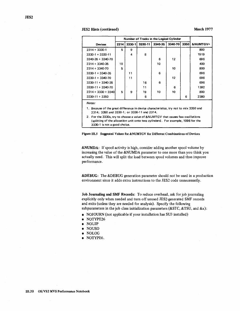
JES2
JES2 Hints (continued) March 1977
Number of Tracks in the Logical Cylinder
Devices 2314 3330·1 3330·11 3340·35 3340·70 3350 &NUMTGV=
2314 + 3330·1 5 9 800
3330·1 + 3330·11 4 8 1919
3340·35 + 3340·70 6 12 696
2314 + 3340·35 10 10 400
2314 + 3340·70 5 10 800
3330·1 + 3340·35 11 6 696
3~30·1 + 3340·70 11 12 696
3330·11 + 3340·35 16 6 696
3330-11 +3340·70 11 6 1392
2314 + 3330 + 3340 5 9 19 10 10 800
3330-11 + 3350 6 6 2380
Notes:
1. Because of the great difference in device characteristics, try not to mix 3350 and 2314; 3350 and 3330-1; or 3330-11 and 2314.
2. For the 3330s, try to choose a value of &NUMTGV that causes few oscillations (splitting of the allocation unit onto two cylinders). For example, 1096 for the 3330-1 is not a good choice.
Figure 111.5 Suggested Values for &NUMTGV for Different Combinations of Devices
&NUMDA: If spool activity is high, consider adding another spool volume by increasing the value of the &NUMDA parameter to one more than you think you actually need. This will split the load between spool volumes and thus improve performance.
&DEBUG: The &DEBUG generation parameter should not be used in a production environment since it adds extra instructions to the JES2 code unnecessarily.
Job Journaling and SMF Records: To reduce overhead, ask for job journaling explicitly only when needed and turn off unused JES2·generated SMF records and exits (unless they are needed for analysis). Specify the following subparameters in the job class initialization parameters (&STC, &TSU, and &x):
• NOJOURN (not applicable if your installation has SU3 installed)
• NOTYPE26 • NOUJP • NOUSO • NOLOG • NOTYPE6.
111.20 OS/VS2 MVS Performance Notebook
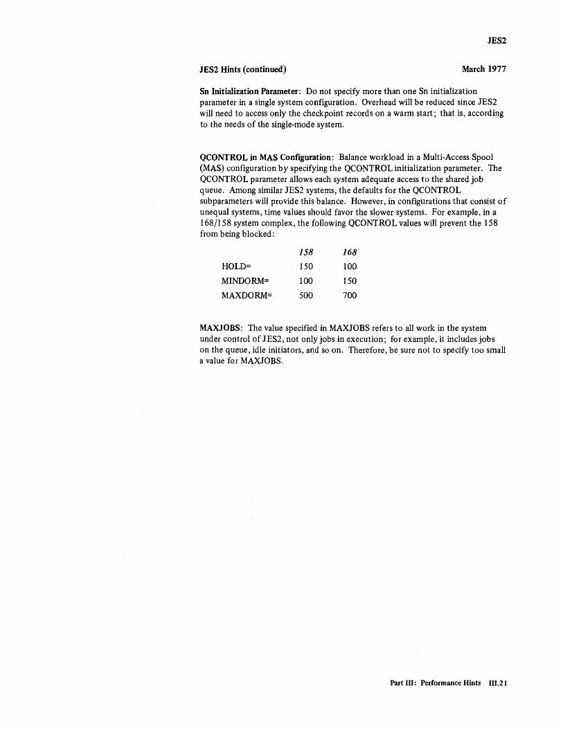
JES2
JES2 Hints (continued) March 1977
Sn Initialization Parameter: Do not specify more than one Sn initialization parameter in a single system configuration. Overhead will be reduced since JES2 will need to access only the checkpoint records on a warm start; that is, according to the needs of the single-mode system.
QCONTROL in MAS Configuration: Balance workload in a Multi-Access Spool (MAS) configuration by specifying the QCONTROL initialization parameter. The QCONTROL parameter allows each system adequate access to the shared job queue. Among similar JES2 systems, the defaults for the QCONTROL subparameters will provide this balance. However, in configurations that consist of unequal systems, time values should favor the slower systems. For example, in a 168/158 system complex, the following QCONTROL values will prevent the 158 from being blocked:
HOLD=
MINDORM=
MAXDORM=
158 168
150
100
sao
100
150
700
MAXJOBS: The value specified in MAXJOBS refers to all work in the system under control of JES2, not only jobs in execution; for example, it includes jobs on the queue, idle initiators, and so on. Therefore, be sure not to specify too small a value for MAXJOBS.
Part III: Performance Hints 111.21

111.22 OS/VS2 MVS Performance Notebook
OS/VS2 MVS Performance Notebook
Part III
Seek Time, Red ucing
Seek Time, Reducing
March 1977
Data Set Placement: Plan the allocation of data sets on each volume to minimize the average distance travelled per seek. Rarely used data sets should be placed at the very beginning or end of the volume, but not under fixed heads. This effectively reduces the size of the active volume. The VTOC should generally be surrounded by the most active data sets and placed 1/3 to 1/2 of the way into the volume. (Examples of heavily used data sets are catalogs and page data sets; LINKLIB data sets are moderately used.) An exception to this guideline is on fixed head units in a 3340-F or 3350. More seeks are saved on these devices if the VTOC is placed within the fix area. Another exception is on volumes such as SYSRES, which are normally accessed by many tasks. On these volumes, the VTOC might be rarely used, and can therefore be considered as just another data set; that is, placement at the end of the pack produces the greatest reduction in seek time. Keep in mind that all data sets should be allocated on cylinder boundaries, where possible.
Module Ordering Within PDSs: Re-order modules within critical partitioned data sets, such as heavily used libraries, according to their frequency of use. This will eliminate seeks within the data set. The following technique can be used to re-order a partitioned data set:
1. Use the SEEKANAL measurement tool or GTF SIO trace records to determine the most frequently used members in the data set.
2. Arrange these modules in groups that will fit within cylinder boundaries. (As it is difficult to calculate the cylinder boundary exactly, prepare IEBCOPY COpy and SELECT statements for each module.)
3. Using the IEBCOPY utility, copy the modules in the preferred order into a temporary data set.
4. Using IEBCOPY without the SELECT statement, copy the whole temporary data set into the new permanent data set. No sorting will take place.
5. Keep the list in PARMLIB for further reference and updates.
Part III: Performance Hints 111.23

111.24 OS/VS2 MVS Performance Notebook

OS/VS2 MVS Performance Notebook
Part III
Shared DASD Hints
Shared DASD
March 1977
Shared DASD, particularly between loosely-coupled systems, can cause generalized, often unnoticed, performance problems. Reducing hardware costs by pooling DASD might actually increase costs by reducing system performance. Although processor utilization might not decrease noticeably (due to additional processor cycles in more frequent task switching), shared DASD can cause application programs to execute more slowly. This can be especially serious in responseoriented systems, such as IMS, CICS, or TSO environments. System throughput can actually degrade by as much as 10-15% due to short duration lockouts and to device or control unit interference and contention.
It is recommended that you share as few DASD strings as possible,consistent with reasonable back-up. When implementing shared DASD, consider the following suggestions and potential problem areas.
Operational Problems in Disk Pack Management (JES2 only): Considerable human intervention might be necessary to keep track of the status of the shared devices. For example, the operators should initiate all shared volume mounting and '.: demounting operations, but these operations must b~ done in parallel on all sharing systems. Valid combinations of volume mount characteristics for all sharing systems must also be maintained. Device availability problems can easily cause jobs to abend or can waste available spindle time. Difficulties like these tend to increase substantially with each additional loosely-coupled system, since requirements for inter-operator coordination and communication become increasingly complex. Keep in mind that the operating procedures at your installation might have to be revised as your uses of shared facilities evolve.
String Switching and Isolating Shared DASD: Consider string switching (the facility available with the 3333 storage control module) for all shared DASD strings. This will provide for maximum availability by backing up the DASD control units in the event of a hardware failure, and might benefit performance by reducing control unit contention. A disadvantage of string switching, however, is that SID operations might return false device busy indications. Since the system cannot distinguish between the devices being busy or the storage control module (string) being busy, it always assumes that the device is busy. All I/O will be queued instead of being scheduled to the optional channel path. A more efficient use of the resources is gained by installing string switching, but inactivating it via the VARY OFFLINE command during normal system operation. This technique will make maximum use of the OPTCHAN feature in MVS.
Part III: Performance Hints 111.25

Shared DASD
Shared DASD Hints (continued) March 1977
Volumes that must be shared, such as catalogs and program library packs, should be isolated from all other types of volumes and placed on a single string of devices where possible. This will isolate shared control unit interference to a single string ofDASD. However, if the string is heavily used, then all systems sharing the DASD might suffer. Another problem exists if a control unit containing shared system files becomes inoperable. It will be necessary to quiesce and IPL all attached systems in order to relocate these essential files· on a working control unit. This has the effect of multiplying the number of IPLs associated with hardware failure times the number of processors. This cost can be very high. However, string switching this DASD string, combined witb optional channel paths into both control units, will provide for preventive maintenance without causing multiple system IPLs, and will reduce control unit contention as well.
Library Maintenance: Library maintenance (such as link edits) to production libraries should be scheduled in light processing hours, if possible, and should always be scheduled on a single processor. This will minimize performance problems caused by contention. And, by eliminating reserve/release interference during busy periods, the possibility of multi-system lock outs will also be minimized.
111.26 OS!VS2 MVS Performance Notebook

OS/VS2 MVS Performance Notebook
Part III
SVC Hints
SVCs
March 1977
Bulletin 2.3.0, "SVC Analysis," in Part II describes how to identify SVCs that are "costly" in terms of processor time and whose "cost" can be decreased - by decreasing the frequency of the SVC or by reducing the SVC's processor time. Following are specific hints.
Authorizing Programs: If a program can be authorized, use APF to authorize it. This will cause validity checking to be bypassed in SVCs (for example, in ENQ/DEQ, GETMAIN/FREEMAIN, WAIT/POST), therefore shortening their path lengths and processor time.
STIMER and TTIMER (SVCs 47 and 46; modules IGCO004F and IGCOO04G): You can reduce the instruction length - and, therefore, the processor time - of these SVCs by placing them in the fixed LP A. STIMER and TTIMER fix themselves before getting a spin lock. However, when placed in the fixed LP A, they recognize prior fixing and branch around their FIX and FREE code. This cuts the number of instructions required to execute each macro approximately in half (from approximately 2000 instructions per call to approximately 1000 instructions) .
Before implementing this hint, consider the following factors: (1) the criticalness of real storage in your system (increases in fixed LP A will decrease the amount of pageable storage available); and (2) how frequently the SVC is issued. (SVC frequencies are reported by GTFSVC, IUP # 5796-PGE.) If the SVC is issued infrequently - for example, five or fewer times per second - the savings in processor time will not be significant.
ENQ/DEQ: If you have shared DASD in your system, ensure that only the devices to be shared are generated as shared during sysgen. The path length of ENQ/DEQ increases Significantly for devices generated as shared.
Part III: Performance Hints 111.27

111.28 OS/VS2MVS Performance Notebook

OS/VS2 MVS Performance Notebook
Part III
TeAM Hints
TeAM
March 1977
TeAM Buffers: Consider the following suggestions when defining TCAM buffers:
• The amount of storage allocated fbr TCAM's buffers should fit into an integer multiple of a page. This is because storage for the buffer unit pool is obtained in page multiples. Buffers, which are fixed in real storage, do not cross these page boundaries. Therefore, it is important that you optimize the amount of storage used (the number of buffers x buffer unit size) to prevent the waste of unallocated space in the pages or the use of too much real storage. You can either utilize the pages fully (by increasing the size of the buffer unit), or minimize the number of pages that are fixed (by decreasing the number of buffers). Generally, the number of buffers actually used will decrease as the size of the buffer unit increases. Therefore, the most effective way to use the pages is usually to increase the buffer unit size via the UNITSIZE parameter on the TSOMCP macro instruction or the KEYLEN parameter on the INTRO macro instruction. This, however, depends on the characteristics of your particular TCAM installation; for example:
The typical peak number of terminal users.
The nature of user activity (amount of terminal I/O, length of messages, and so on). The amount of terminal I/O can be measured using GTF. In general, for TCAM EP, there should be at least 1.7 buffers per line; NCP requires fewer.
- The type of terminals. Larger buffers are recommended for display stations.
Specify unit size in multiples of 8 plus 4 (for example, 36,44, and so on): TCAM adds 12 bytes to each unit for CCWs and control information, and units begin on a doubleword boundary .
• TCAM 2701/2/3 or 3705 EP only: Since a larger buffer size causes additional buffers to be needed less frequently, PCI processing (which allocates buffers dynamically when the initial buffer specification is insufficient) is also reduced. However, you might want to eliminate PCI interrupts completely by specifying that TCAM perform a static buffer allocation (by coding PCI=(,N». Static buffering causes TCAM to get all the buffers it is going to need prior to issuing the I/O for polling or for addressing. Processor cycles required to process the PCI interrupt are thus saved. However, keep in mind that if you do not use PCI buffering, you will need more buffers and can also experience a slower response time.
Part III: Performance Hints 111.29
TCAM
TCAM Hints (continued) . March 1977
• For non-TSO or mixed TSO/non-TSO TCAM, input and output buffer sizes should be equal. That is, the output buffer size specified on the DCB, GROUP, or TERMINAL macro instruction should be the same as the buffer size on the queue. (The buffer size on the queue is determined by the input buffer size specified on the DCB, adjusted by special editing performed in the message handler.) When the buffer sizes are identical, TCAM can read the message from the queue in the fewest number of queue accesses and no data movement will occur while buffers are being built.
Note: Buffer size on the queue does not refer to disk record lengths or blocksize.
• Data is transferred between TCAM and TSO buffers on input and output in units of TCAM buffer unit size or TSO buffer size, whichever is smaller. To reduce the number of QTIP SVCs to effect the transfer of data, the TCAM unit size and TSO buffer size should be as large as possible.
• On the PCB macro instruction for an application program using disk queueing, code BUFOUT = 2X + 1, where X is the number of TCAM buffers needed to hold the largest anticipated message. The buffers allocated for BUFOUT . constitute the application program read-ahead queue. Messages are read from the disk message queue into these buffers in anticipation of a GET or READ request from the application. If BUFOUT is too small, the result might be delays in satisfying application GETs or READs.
Blocksize of Checkpoint Data Set: The blocksize of the checkpoint data set should be as large as possible. The larger the blocksize, the more efficient checkpoint becomes; the maximum blocksize of 3520 should be used if sufficient storage is available. Checkpoint execution time can also be reduced by making the nonresident checkpoint routines resident. (Use the function-to-module list in OS/VS2 TCAM Logic to determine which routines to make resident.)
TCAM Fixed Storage: TCAM performance is degraded if insufficient storage is available; conversely, storage is wasted if too much is specified. You can determine the amounts of the various storage pools (buffer units, CPBs, main-storage queue units, PLCBs) actually used by TCAM by examing TCAM dumps, as described in OS/VS TCAM User's GUide.
In all environments, ensure the maximum utilization of the fIxed storage used by TCAM. Since TCAM long-term fIxes many of its control blocks, buffers, CPBs, and so on, it is important to make effective use of fIxed storage. Storage is fIxed in 4K pages; buffers, CPBs, and some control blocks cannot cross page boundaries. TCAM keeps track of unused allocated storage and packs control blocks into these areas. If the unused storage is fragmented or if more than one page is needed, additional pages may be allocated and fixed by TCAM unnecessarily. The number of fIxed pages required for TCAM's control blocks can be reduced by reordering the opening of line groups and limiting the number of lines per line group. This and other techniques designed to minimize fixed pages and page faults are described in OS/VS2 System Programming Library: Initialization and Tuning Guide.
111.30 OS/VS2 MVS Performance Notebook

TCAM
TCAM Hints (continued) March 1977
Queuing: If an MCP supports both batch and interactive processing concurrently, use separate queuing structures for batch processing and interactive processing, (for example, non-reusable for batch and reusable for interactive, or vice versa). Otherwise, contention for the disk queue volumes might adversely affect interactive response time.
When disk queuing is being used, the message queues should be separated from system data sets or other high volume data sets. The interaction with high volume data sets of any kind results in the disk not being able to handle the traffic; response time slows down. Using main storage queuing is one way to avoid disk and channel contention for the queuing medium.
Changes in network definition can also be used to improve response time. When a terminal runs in batch mode part of the day and in interactive mode the rest of the day, you can define the same physical terminal twice tomaintain the queuing medium separation. The interactive terminal can use one disk queue (for example, the reusable queue) and the batch terminal can us~ the other (for example, the non-reusable disk queue). Operator control can be used to start and stop the correct logical terminal.
Consistency in Response Time: Consider use of the following features to improve consistency in response time:
• The HOLD macro instruction, which suspends transmission to a particular terminal for a specified time and then retransmits the message that was held. It should be used to prevent an inoperative terminal from tying up the entire line. It must be used if message recovery after a permanent error is desired. A common error is coding too short an interval on the HOLD macro, causing frequent retry of a send operation. This can waste a lot of processor and line time if the terminal is permanently out of order.
• For 270x or 3705 EP:
The MSGLIMIT macro instruction, which controls how many messages are sent to or received from any given terminal on a line. Use of this macro enhances transmission priorities.
The SLOWPOLL and IEDPSTOP macros, which are used to control polling during error conditions by preventing excessive messages to LOGREC and the console when a line fails.
- Poll delay, which delays receiving for a specified time after an unproductive pass through the polling lists. However, for 270x or 3705 EP lines eligible for autopoll, do not code a poll delay. Without poll delay, polling continues on the line without any interruption of the processor until either a positive response is received or a line error occurs. With poll delay, the processor will be interrupted after a single pass through the polling list, and I/O must be restarted via EXCPVR after expiration of the interval. Note that CPRI=S must be coded if poll delay=O.
Part III: Performance Hints 111.31

01.32 OS/VS2 MVS Performance Notebook

OS/VS2 MVS Performance Notebook
Part III
VSAM Catalog Hints
VSAM Catalog
March 1977
The following are general performance-related hints that should be considered when converting to VSAM user catalogs. For further details and additional suggestions on catalog conversion and VSAM catalog performance factors, see the Conversion Notebook and the Initialization and Tuning Guide.
• For the conversion of large as CVOLs, use the CNVTCAT command only to produce the list of catalog entries. Load the VSAM catalog via the DEFINE command. The CNVTCAT command will not use the full space allocated in your VSAM catalog since the addition of entry names in ascending order causes control interval splits in the high-key range.
• Be sure to specify a value for secondary allocation when defining the space requirements for VSAM catalogs. If none is specified, a "catalog full" message can appear when only 25% of the catalog is utilized.
• Adjust the VSAM catalog buffer space in the DEFINE USERCATALOG and DEFINE MASTERCATALOG commands according to the amount of fixed storage available in your system. Although the storage consumption will be high, a large buffer space will speed up processing since more requests can be serviced concurrently. Also, a sufficiently large master catalog buffer space will maximize the number of concurrent searches of the master catalog and each jobshared user catalog.
• Use one catalog for each major group of users or applications. Having multiple user catalogs shortens the time required to search for an entry and reduces contention for the catalogs. Thus, both processor time and wait time is saved. In addition, backup and recovery is made easier. However, in systems where storage is a critical resource, too many user catalogs can delay response time. Although only 200-400 bytes of real storage have to be page fixed for each catalog, you should consider sharing more user catalogs in storage-constrained systems that are experiencing unsatisfactory response time.
• Mount the catalog volume on a non-shared device so that catalog records in buffers can be reused.
• If your installation is using GDGs in VSAM catalogs, you can prevent a performance problem from developing by allowing extra space in the high-key range of the catalog. Poor utilization of the high-key range can result from the addition of entry names in ascending order because the space occupied by old, deleted generation names is not always reused as it is in CVOLs.
If your installation has SU8 installed, however, you can create new GDGs and catalog them in either VSAM catalogs or as CVOLs. Performance might be improved by building new index levels and GDGs in the CVOLs instead of in VSAM catalogs.
Partlll: Performance Hints 111.33

lll.34 OS/VS2 MVS Performance Notebook

ACR (alternate CPU recovery) not specifying if not MP 11.56
address spaces, dominant (see dominant users)
address space control block (ASCB) as source of performance data 1.33
allocation considering in place of VIO 11.59 of data sets, to minimize seek time 111.23
allocation recovery possibility oflong wait swaps 11.53
alternate CPU recovery (ACR) not specifying if not MP 11.56
amount of work, documenting 1.9-1.10 analysis, performance problem
"alternative" solutions 11.8 basic performance factors, reviewing 11.6
(see also basic performance factors) describing problem 11.4 focus dictated by type of problem 11.6 measurements, collecting 11.5-11.6 overview of steps 11.3-11.8
summary of steps 11.3 remeasuring and re-evaluating 11.3 system-oriented performance problems 11.7
focusing on major resources 11.7 (see also I/O resources, investigating; processor time,
investigating; real storage, investigating) user-oriented performance problems 11.8,11.63-11.78
APF (authorized program facility) (see authorizing programs)
APG suggestions for 111.15 using to increase work's access to the processor 11.70
application accounting report of IMS/VS Statistical Analysis Utility Program
used in computing ratio of data-base SIOs to DB calls or transactions 11.4 7
applications, batch (see batch work)
ASCB as source of performance data 1.33
ASM processing approximate non-TCB processor time for
for swap paging 11.15 for non-swap paging 11.15
ASM queue length modifying happy range to reduce IMS paging 111.14
ASM vector table (ASMVT) as source of performance data 1.32
ASMVT (ASM vector table) as source of performance data 1.32
authorized program facility (APF) (see authorizing programs)
authorizing programs to reduce SVC path lengths 111.27
automatic priority group (see APG)
auxiliary storage manager processing (see ASM processing)
auxiliary storage manager vector table as source of performance data 1.32
auxiliary storage shortage swaps, reducing 11.53 available frame queue
Index
invalid as indication of real storage problems 11.49 average time of ended transaction (TSO)
reported by RMF or MF/l 1.7-1.8 factors not included in measurement 1.8
average time to service an I/O request, computing 11.39 indicating possibly critical I/O path 11.37
basic performance factors dominant users 1.4 7 hardware configura tion 1.47 I/O resource balancing 1.47 operational bottlenecks 1047-1.49 reviewing as part of analysis 11.6
basic sequential access method (see BSAM)
batch job classes (see job classes)
batch environments (see batch work)
batch processing TCAM queueing for 111.31
batch turnaround measuring 1.9
batch throughput measuring 1.9 setting throughput limits 1.12
batch work access to processor, investigating possible problem of 11.69 additional real storage vs. 2305 111.11 comparison of ASM-queue-Iength and VIC happy
values in IMS/batch and TSO/batch systems 111.14 demand paging target values 11.52 dispatching priority hints 111.15 enqueue contention, investigating possibility of 11.75 factors to include in documenting workload 1.10 MPL hints for batch domains 111.17 real storage guidelines 111.9 reducing EXCPs for 11.49 sample performance objective 1.13 waiting for I/O, investigating possibility of 11.73 waiting to start, investigating possibility of 11.72
BFPLBFSZ operand specifying block size to eliminate ISAM/OSAM data
base compaction 11.48 BLDL lists
using GTF data to create 1.44 block multiplexor channels
judging utilization of 11.38 (see also channels, investigating)
tape devices on 111.11 blocksizes
hints 111.3-111.4 benefits and trade-offs 111.3 DASD 1I1.3-IIIA procedure libraries IliA program libraries 111.4 tape devices 111.3 TCAM checkpoint data set 111.30 unit record devices 111.3
increasing to reduce EXCP counts 11.47 possible solution to I/O delays 11.33-11.34 specifying to eliminate ISAM/OSAM data base
compaction 11048
Index i.l

BLKSIZE (see blocksizes)
bottlenecks iden tifying
(see analysis, performance problem) BSAM (basic sequential access method)
versus QSAM on DASD 111.3 on unit record devices 111.3
BSP and QSAM to tape 111.3
buffer pool size (see buffers, number of and size)
buffers, number of and size general hints 111.3-111.4
benefits and trade-offs 111.3 DASD 111.3-111.4 procedure libraries 111.4 tape devices 111.3 unit record devices III.3
IMS message queue data set, insufficient 11.66 increasing to reduce IMS SIOs 11.48 JES2 111.19 output TIOC buffers, insufficient
causing output terminal wait swaps 11.53 TCAM II 1.29-111.30 VSAM catalog 111.33 VSAM data bases, specifying to reduce data base SIOs 11.48
BUFNO (see buffers, number of and size)
BUFSIZE JES2 hints 111.19
BURST mode devices optional channel balancing to 111.5
capacity limits, setting 1.12 capacity management aid
(see CMA) catalogs
(see VSAM catalogs) catalog structure
possible solution to enqueue contention 11.75 categories of processor time 11.9-11.11
focusing on different categories 11.11-11.12 categories of work
defining 1.9 measuring resources used 1.11-1.12 setting capacity limits 1.12 setting resource limits 1.12
CCH records as source of performance data 1.40
chained scheduling reducing EXCPs 111.3
channel activity report, RMF or MF/1 used to compute channel time per access 11.41-11.42 used to identify critical I/O paths 11.37-11.39 used to investigate possibility of I/O delays for IMS
work 11.73 used to monitor performance 1.45
channel bottlenecks (see channels, investigating)
channel monopolization buffer pool considerations 111.3
channels balancing activity between optional and primary paths 111.5 balancing, as solution to I/O delays 11.33-11.34
(see also channels, investigating) control blocks that contain information on 1.29 judging reasonableness of pre-MVS configuration
for MVS 111.8 tools that report on 1.29
i.2 OS/VS2 MVS Performance Notebook
channels, investigating channel measurements indicating potentially critical I/O
paths "percent channel busy" measurement 11.37,11.38 "percent channel busy and CPU wait"
measurement 11.37-11.38 combining with "CPU wait" measurement 11.38
focusing on specific channel bottlenecks contention caused by reconnects from RPS de vices 11.4 2 high channel time per access 11.41-11.42
checkpoint, TCAM blocksize of checkpoint data set 111.30 making routines resident 111.30
CICS environment possible impact of shared DASD III.25
classes, job (see job classes)
CMA general information 1.17 input to and output from 1.20 operational considerations 1.23 types of data provided 1.25
CNTRL macro instruction vs. control characters on unit record devices 111.3
CNVTCAT command of access method services versus DEFINE command for converting OS CVOLs 111.33
coefficients reflecting relative time to perform SCP functions on different processor models 11.17
used in converting SVC time measured on one processor to approximate time on different processor 11.22
used in formulas for breakdown of non-TCB time 11.15 - 11.19 commands
identifying those with high TCB time 11.29 lack of SVC information for 11.29
common data set examining placement to reduce time to resolve page-in 11.61
common storage area (see CSA)
compaction, data base, eliminating 11.48 condition codes, SIO
(see SIO condition codes) configuration
basic performance factor 1.4 7 documenting when taking measurements lAO I/O
optional channels 111.5 reducing I/O bottlenecks 11.45 (see also channels, investigating; control units; devices,
investigating) multi-access spool configuration
specifying QCONTROL 111.21 reviewing adequacy during analysis 11.6 rules-of-thumb 111.7-111.10
I/O resources 111.8 processor 111.7-111.8 real storage 111.8-111.10
2305 vs. additional storage 111.11 3270s and tapes 111.11
contention (see data base segment contention; enqueue contention;
latch contention; lock contention) control blocks
as source of performance data 1.30-1-34, 1.28-1.29 ASCB 1.33 ASMVT 1.32 chaining of 1.31 OUCB 1.33-1.34 OUXB 1.34 PFT 1.32 PVT 1.32 RMCT 1.32 SPCT 1.33
IMS, insufficient stroage assigned for 11.65 TCAM, fixed storage for 111.30
control characters vs. CNTRL macro on unit record devices 111.3
control interval size of VSAM data base requesting empty control interval 11.48 specifying buffers to match 11.48
control of users that monopolize resources basic factor to review during analysis 11.6
control region, IMS unable to schedule transactions 11.65
control units balancing, possible solution to I/O delays 11.33-11.34 bottlenecks, investigat ing 11.4 2-11.4 3 contention on shared DASD 111.25
isolating volumes to reduce 111.26 string switching to reduce 111.25-111.26
tools that report on 1.29 control volumes
(see CVOLs) CPBs
fixed storage for 111.30 CPU
(see processor) CPU activity report, MF/l or RMF
measurement of wait time 11.7 using to monitor performance 1.45
CSA (common storage area) demand paging in, reported by SIR 11.57 paging, important factor for IMS 11.71 real storage guidelines 111.9 reducing to reduce fixed storage 11.56
CSECT ordering possible solution to excessive paging 11.72 to achieve efficient page reference patterns 11.57
CVOLs converting to VSAM catalogs
catalog buffer size II1.33 DEFINE vs. CNVTCA T command 111.33 GDGs in 111.33 mounting on non-shared DASD 111.33 multiple user catalogs 111.33 secondary allocation 111.33
cylinder boundaries allocation on III .23 calculating cylinder boundary 111.23
D M command as source of data 1.30
DACA general information 1.17 input to, output from, and overhead of 1.20 operational considerations 1.23 types of data provided 1.26
DASD blocksize and buffer hints
trade-offs 111.3 hints 111.3-111.4
JES2 buffer sizes 111.19 RPS
effect of channel scheduling on 111.5 judging reasonableness of channels to RPS in MVS
system 111.8 seek time, reducing
data set placement 111.23 module order within PDS 111.23
shared (see shared DASD)
steps in satisfying I/O requests and their performance implica tions 11.33-11.34
tools that report on 1.29 &NUMTGV, suggested values for 111.19-111.20 (see also devices, investigating)
data base compaction, eliminating 11.48
data base mapping programs, IMSMAP/VS general information 1.19
data reduction programs available from IBM
data provided by 1.24-1.26 general information 1.15-1.19 input to, output from, and overhead of 1.20-1.21 operational considerations 1.22-1.23
user-written control blocks 1.30-1.34 GTF 1.41-1.42,1.43-1.45 SMF 1.41-1.43 trace table 1.35-1.40
data base reorganization to reduce IMS SIOs 11.48
data base segment contention possible cause of user-oriented performance problem 11.63
investigating 11.75 possible solutions 11.75
data base SIOs, reducing 11.4 7-11.48 data set allocation
to minimize seek time 111.23 data set placement
page and swap data sets affecting swap-in time 11.66
possible solution to I/O delays 11.39-11.45,11.33-11.34 to minimize seek time 111.23 using GTF to examine 1.44
data sets understanding characteristics to red uce I/O
bottlenecks ·11.45 utilization, caution when reducing I/O bottlenecks 11.45
data transfer possible source of delay in satisfying I/O
requests 11.33-11.34 DB/DC applications
executing as non-swappable 11.78 DB/DC environments
(see IMS work) DC attribute on modules, removing 111.4 DC Monitor
(see IMS DC Monitor) DDR records
as source of performance data 1.40 DEBUG JES2 parameter, hint 111.20 DEFINE command of access method services
versus CNVTCA T command for converting OS CVOLs 111.33
demand paging computing non-TCB time for VIO and demand
paging 11.15-11.19 formula for 11.18
effect of 2305 vs additonal storage 111.11 excessive, possible cause of user-oriented performance
problem 11.63 investigating problem 11.71-11.72 possible solutions 11.72
focusing on if paging causing wait time 11.51-11.52
target values for 11.52 if paging costing non-productive processor time 11.51 if paging I/O interfering with other I/O 11.49-11.51 judging rates 11.49
in IMS-mixed environments 111.13-111.14 reducing 11.55-11.58
localizing page references 11.56-11.57 reducing fixed storage 11.56 reducing multiprogramming level 11.58 separating users with large working sets 11.57-11.58 steps to reduce 11.55
target values for 11.52
Index i.3

DEQ (SVC 48) path length for shared DASD 111.27 path length when executed by a uthorized program 111.27
detected wait swaps possible indication of enqueue contention 11.75 reducing 11.54
device activity report, MF 11 or RMF used to compute device time per access 11.41-11.42 used to compute SIOs to data base 11.47 used to identify critical 1/0 paths II.37-1I.39 used to identify device bottlenecks 11.41 used to investigate possibility of I/O delays for IMS
work 11.73 used to monitor performance 1.45
device bottlenecks (see devices, investigating)
devices, investigating device measurements indicating potentially critical 110 paths
"average time to service a request" 11.37, 11.39 "queue length" measurement II.37, 11.38-11.39
focusing on specific device bottlenecks 11.41 excessive seek time 11.41 questionable significance of "device busy"
measurement 11.41 tools that report on devices 1.29 (see also DASD; shared DASD; tape devices; unit record devices)
DFSILTAO (see IMS/VS transaction analysis utility program)
DFSPIRPO (see IMS/VS program isolation trace report utility program)
DFSVSAMP data set . specifying blocksize to eliminate ISAM/OSAM data base
compaction 11.48 direct access contention analyzer
(see DACA) direct access storage devices
(see DASD) disk queueing for TCAM 111.31 dispatcher
processor time not recorded by. 11.10-11.11 dispatching priority (DPRTY)
assigning preferred priority to solve enqueue contention 11.75
hints 111.15 increasing, as solution to work waiting for the
processor 11.70 display matrix command
as source of data 1.30 display stations
TCAM buffer size 111.29 distribution of system output
opera tional bottleneck 1.49 domain constraints
(see domains weights; domains) domain weights
affecting swap-in of TSO transactions 11.66 changing MPLs vs domain weights 111.17 importance of 111.17 possibly causing swap-in delay 11.78
domains computing TCB time for 11.13-11.14 controlling non-IMS work to reduce IMS demand
paging 111.14 domain control hints 111.17
batch domains 111.17 MPLs vs domain weights 111.17 TSO domains 111.17
i.4 OS/VS2 MVS Performance Notebook
domains (continued) placing TSO trivial and non-trivial transactions in separate domains 11.66-11.67
using to make address spaces nonswappable 11.10 dominant users
basic per formance factor 1.47 identifying heavy processor users 11.29-11.31 investigating paging for 11.71
DPRTY (see dispatching priority)
ended transactions field in RMF or MF 11 deriving TSO transaction rate from 1.8
ENQ (SVC 56) path length for shared DASD 111.27 path length when executed by authorized program 111.27
enqueue contention causing detected wait swaps 11.54 causing enqueue exchange swaps 11.54 causing long wait swaps 11.53 possible cause of user-oriented performance problem 11.63
investigation and possible solutions 11.75 enqueue exchange swaps
possible indication of enqueue contention 11.75 reducing 11.54
environment documenting when taking measurements 1.40
error statistics as source of performance information 1.40-1.41
evaluation, performance steps 1.1-1.2
exchange-on-recommendation-value swaps, reducing 11.54 exchange swaps
(see enqueue exchange swaps; exchange-on-recommendationvalue swaps)
EXCPs increased path length in MVS 111.3 rates on MVT, as basis for judging adequacy of
processor 111.7 reducing 11.4 7 -11.48
benefits of 11.47 blocksize and buffer hints 111.3-111.4 focusing on data sets with high EXCP rates 111.3 focusing on users with high EXCP rates 11.4 7 for batch work 11.47 for IMS work 11.47-11.48 for TSO work 11.47 JES2 buffer size 111.19 possible solution to 1/0 delays 11.33-11.34 to paging data sets 11.47
tools that report on 1.29 EXCP/XDAP (SVC 0)
example of computing TCB time for 11.23 expectations, system
(see performance objectives)
FBS (fixed block standard) hints for DASD 111.4
FDPs general information 1.15-1.19 input to, output from, and overhead of 1.20-1.21 operational considerations 1.22-1.23 types of data provided 1.24-1.26
Field Developed Programs (see FDPs)
fixed block standard (see FBS)
fixed-head DASD VTOC placement on 111.23

fIxed storage maximum utilization by TCAM 111.30 reducing
approach to reducing 11.56 as step in reducing demand paging 11.55
VSAM catalog buffer space 111.33 VSAM user catalogs 111.33
focus of tuning effort dictated by type of objective not met 11.6-11.8
forms mounting operational bottleneck 1.49
formulas average number of pages per SIO 11.17 average time to service an I/O request 11.39 batch processor utilization 1.12 channel time per access 11.41-11.4 2 device time per access 11.41-11.42 EXCP/SIO rate 11.47 for estimating maximum MPL for TSO 111.17 for estimating processor utilization on MVS, based on MVT
utilization 111.7 MSO service 11.57 non-TCB time breakdown 11.15-11.19
example of using formulas 11.19 non-swap non-paging I/O interrupt non-TCB time 11.18 non-swap paging non-TCB time 11.18 summary of formulas 11.16 swapping non-TCB time 11.17 total non-TCB time 11.15
checking accuracy 11.16-11.17 percentage of processor wait time during which channel is busy 11.37-11.38
problem program time for ajob, if SVC time is computed 11.31
SVC processor cost as percentage of processor utilization 11.22 as percentage of total TCB time 11.22
SVC time for specifIc job 11.29-11.31 TCB percentage of job TCB time for specific SVC 11.31 TCB time from RMF 11.13 time to resolve page-in 11.61 TSO processor utilization 1.12 TSO transaction rate 1.8 working set size from RMF 11.57 working set size from SMF 11.57-11.58
frames, number of available invalid as indication of real storage problems 11.49
FREE=CLOSE JCL parameter possible solution to enqueue contention 11.75
front end of SVCs dermed 11.10 (see also SVC usage)
generalized trace facility (see GTF)
generation data groups (GDGs) in VSAM catalogs 111.33
GETMAIN/FREEMAIN (SVC to) example of computing TCB time for 11.23 path length when executed by authorized program 111.27
GDGs (generation data groups) in VSAM catalogs 111.33
goals set for system (see performance objectives)
GTF general information 1.17 input to, output from, and overhead of 1.20 operational considerations 1.22
GTF (continued) reduction programs available from IBM
general information 1.17-1.19 input to, output from, and overhead of 1.20-1.21 operational considerations 1.23 types of data provided 1.25-1.26
requesting time-stamping 11.5 types of data provided 1.24 used to break down swapped-out time 11.78 used to collect basic set of measurements 11.5 used to deterinine why swaps are occurring 11.77 used to identify SVCs called by specificjobs/logons 11.29 used to investigate wait-to-start time for TSO 1I~66
used to break down wait-to-start time 11.66 used to measure nature of TCAM user activity 111.29 used to obtain "cost" of SVCs 11.21-11.22 used to obtain frequency of SVCs 11.21 used to order modules within PDS 111.23 writing data reduction program for 1.41-1.42,1.43-1.45
GTFANAL general information 1.17 input to, output from, and overhead of 1.21 operational considerations 1.23 types of data provided 1.26
GTF data analysis program (see GTFANAL)
GTF direct access contention analyzer (see DACA)
GTF I/O concurrency tool (see GTFIOCUR)
GTFIOCUR general information 1.17 input to, output from, and overhead of 1.20 operational considerations 1.23 types of data provided 1.26 used to report SIO condition codes 11.42
GTF supervisor services analyzer (see GTFSVC)
GTFSVC general information 1.17 input to, output from, and overhead of 1.20 operational considerations 1.23 types of data provided 1.25 used to identify SVCs used by a job 11.29
meaning of "job" for GTFSVC 11.29 used to obtain frequency of SVCs 11.21
GTFVTAM general information 1.17 input to, output from, and overhead of 1.20 operational considerations 1.23 types of data provided 1.26
GTF VT AM buffer trace analysis tool (see GTFVT AM)
guidelines (see formulas; rules-of-thumb; target values)
happy values for SRM indicators of system contention changing to achieve lower multiprogramming level 11.58 changing to reduce IMS paging 111.14
hardware additional
as solution to performance problems 11.8 possibly indicated by storage shortage swaps 11.53
configuration basic performance factor 1.47 (see also cOnIlguration)
Index i.S

hardware monitors general information 1.18 input to, output from, and overhead of 1.21 operational considerations 1.23 source of data on system-wide resource utilization 11.5 types of data provided 1.26
HOLD macro instruction to improve consistency in TSO response time 111.31
HOLD subparameter of QCONTROL parameter specifying for MAS configuration 111.31
identifying and reducing non-productive processor time 11.9-11.31
breakdown ofnon-TCB time' 11.15-11.19 categories of processor time 11.9-11.11 computing TCB time 11.13-11.14 focusing on different categories 11.11-11.12 identifying heavy processor users 11.29-11.31 SVC analysis 11.21-11.27
IEAFIXxx member of PARMLIB reducing fIxed storage 11.56
IEBCOPY used to re-order PDS 111.23
IFCEREPO service aid as source of performance data 1.41
IGC0004F (see STIMER)
IGD0004G (see TTIMER)
IKJPRMxx member of PARMLIB OW AITHI value 11.53
IMSASAP general information 1.19
IMS control region (see control region, IMS)
IMS DC monitor general information 1.18 indicating possible I/O contention 11.73 used in computing ratio of data-base SIOs to DB calls or transactions 11.48
IMS environment (see IMS work)
IMS latches possible cause of user-oriented performance problems 11.63
IMS log tape analysis tool general information 1.19
IMSMAP/VS data base mapping programs general information 1.19
IMS measurement tools general information 1.18-1.19
IMS monitor summary and system analysis program (see IMSASAP)
IMS response time analyzing
(see user-oriented performance problems, analyzing) measurement of 1.8
IMS transactions as reported on transaction response report 1.8 factors to include in documenting workload 1.10
IMS utilities (see IMS DC Monitor; IMS/VS log transaction analysis u~ty program; IMS/VS program isolation trace report utility program; IMS/VS statistical analysis utility program)
IMS work access to processor, investigating possible problem of 11.69 data l?ase segment conteiltion, investigating possible problem
of 11.75 .
i.6 OS/VS2 MVS Performance NQtebook
IMS work (continued) demand paging for
in IMS-mixed environment 111.13-111.14 target values 11.52
effect of pre-load 11.52 documenting workload, factors to include in 1.10 EXCPs for, reducing 11.47-11.48
examining ratio of data-base SIOs to DB calls or transactions 11.4 7 -11.4 8
ways to reduce 11.48 input queue time, investigating as possible
delay 11.65-11.66 not executed in APG 111.15 real storage guidelines 111.9 reducing fIxed CSA for 11.56 shared DASD, possible impact of 111.25 significant paging factor for 11.71 waiting for I/O, investigating as possible delay 11.73
IMS/VS DC Monitor (see IMS DC Monitor)
IMS/VS log transaction analysis utility program general information 1.18 used to investigate input queue time 11.65 used to investigate possible problem ·of work waiting for the
processor 11.69 IMS/VS program isolation trace report utility program
general information 1.18 used to investigate possible data base contention 11.75
IMS/VS statistical analysis utility programs general information 1.18 measurements of IMS response time 1.8 used to compute ratio of data-base SIOs to DB calls or
transactions 11.4 7 used to investigate possible problem of work waiting for
the processor 11.69 IMS/VS virtual storage analysis tool
general information 1.19 "index-in-core" option for ISAM
reducing IMS SIOs 11.48 initialization parameters
addressing as basic performance factor 1.4 7 JES2, hints 111.19-111.21
initiators, number of as possible solution to excessive wait-to-start time 11.65 controlling non-IMS work to reduce IMS demand
paging 111.14 operational bottleneck 1.48
input buffers size for TCAM 111.30
input of work into system operational bottleneck 1.49
input queue time, excessive (see waiting to start)
input terminal wait swaps, reducing 11.53 Installed User Programs
(see IUPs) introduction to performance evaluation 1.1-1.2 investigating the use ofI/O resources
(see I/O resources, investigating) investigating the use of processor.time
(see processor time, investigating) investigating the use of real storage
(see real storage, investigating)

I/O activity measured by SMF 1.43 measuring via GTF 1.44 tr acing, as part of basic set of measuremen ts 11.5 (see also I/O resources)
I/O bottlenecks (see I/O resources, investigating)
I/O device activity report (see device activity report, MF/1 or RMF)
I/O interrupts approximate non-TCB time for processing 11.15 non-swap, non-paging
computing processor time for 11.15-11.19 formula for 11.18
non-swap paging computing processor time for 11.15-11.19
formula for 11.18 I/O requests
steps in satisfying and their performance implications 11.33-11.34
I/O resources as factor in documenting workload 1.10 balancing
basic performance factor 1.4 7 configuration
guidelines for MVS 111.8 optional channels 111.5
control blocks that contain information on 1.29 I/O resources, investigating 11.33-11.48
delays in satisfying requests, overview 11.33-11.34 focusing on specific I/O bottlenecks 11.41-11.43 identifying critical I/O paths 11.37-11.39 paging I/O interfering with other I/O 11.49-11.51 reducing bottlenecks in I/O paths 11.45 reducing EXCPs/SIOs 11.47 summary of process to investigate 11.35 when to investigate 11.33
I/O, waiting for possible cause of user-oriented performance problems 11.63
investigation and possible solutions IMS 11.73 TSO or batch work 11.73
I/O trace records providing information on I/O activity 1.44
IPS performance objective affect ing unilateral and exchange-on-recommendation
value swaps 11.54 assigning preferred objectives to work to solve enqueue
contention 11.75 distinction from system expectations 1.5 possibly affecting swap-in-delay
after swap-out 11.78 waiting to start for TSO 11.66-11.67
specifying to ensure pre-emption 11.67 IPS specification
(see IPS performance objective) ISAM data bases
ways to reduce data base SIOs 11.48 ISAM "index-in-core" option
reducing IMS SIOs 11.48 iterative nature of performance analysis 11.3 IUPs
general information 1.15-1.19 input to, output from, and overhead of 1.20-1.21 operational considerations 1.22-1.23 types of data provided 1.24-1.26
IWAIT time, high indicating possible I/O contention 11.73
JCL parameter FREE=CLOSE possible solution to enqueue contention 11.75
JESGEN JES2 generation and initialization parameter
hints 111.19-111.21 JESGEN listing
as source of data 1.30 JES2
buffer size hints 111.19 job journaling and SMF records 111.20 not run in APG 111.15 QCONTROL in MAS configuration 111.21 real storage guidelines 111.9 Sn initialization parameter 111.21 &DEBUG hint 111.20 &NUMDA hints 111.20 &NUMTGV hints 111.19-111.20
JES2 generation (see JESG EN)
JES2 initialization (see JESGEN)
JES3 real storage guidelines 111.9 SDEPTH parameter
affecting volume mounting 1.20 JES3 monitoring facility
(see JMF) JIA
general information 1.17 input to, output from, and overhead of 1.20 operational considerations 1.23 types of data provided 1.25
comparison to SUDP and SIR 1.27 JMF
general information 1.18 job class initialization parameters
subparameters to specify to reduce overhead 111.20 job classes
factors to include in documenting workload 1.10 installation controls on 1.12 restructuring
as possible solution to excessive wait-to-start time 11.65 sample objective for 1.13
job entry subsystem (see JES2; JES3)
job journaling hint 111.20 jobstream tuning
using SMF data for 1.42 job termination SMF record
(see type 5 SMF record) journaling hint, job 111.20
latch contention possible cause of user-oriented performance problems 11.63
link pack area (see LPA)
local system queue area (see LSQA)
lock contention possible cause of user-oriented performance problems 11.63
logical channel paths balancing activity within physical path 111.5
LOGREC data set preventing excessive messages when line fails 111.31 source of performance information 1.40-1.41
log transaction analysis utility program (see IMS/VS log transaction analysis utility program)
Index i.7
long wait swaps possible indication of enqueue contention 11.75 red ucing 11.53
LP A (link pack area) fixed, reducing 11.56 real storage guidelines Ill. 9
LSQA (local system queue area) fixed frames for 11.56 real storage guidelines 111.9
main storage service (see MSO serVice)
MAS configuration specifying QCONTROL 111.21
master catalog (see VSAM catalogs)
master scheduler not run in APG 111.15 real storage guidelines 111.9
MAX DORM parameter of QCONTROL parameter specifying for MAS configuration 111.21
maximum CPU service units per second 11.14 maximum MPL
affecting swap-in of TSO transactions 11.66 for batch 111.17 for TSO domains 111.17
MAXJOBS possible effect of &NUMTGV on 111.19 specifying 111.21
MCR records as source of performance data 1.40
mean-time-to-wait subgroup of APG (see MTTW subgroup of APG)
measurement tools executing on regular basis
for monitoring performance 1.45-1.46 to identify usual values of measurements 11.5
importance of 1.15 monitoring performance 1.45-1.46 other sources of MVS data 1.30-1.41
control blocks 1.30-1.34 SYS1.LOGREC 1.40-1.41 trace table 1.35-1.40
overview of IBM MVS measurement tools 1.15-1.30 comparison of SIR/SUDP/JIA 1.27 general information 1.17-1.19 input to, output from, and overhead of 1.20-1.21 operational considerations 1.22-1.23 sources of data on system resources 1.28-1.29 types of data provided 1.24-1.26
writing data reduction programs 1.41-1.45 GTF data 1.41-1.42, 1.43-1.45 SMF data 1.41-1.43 trace table 1.35-1.40
measurements basic set to begin analysis 11.5-11.6
judging values of specific measurements 11.5 types of information to collect 11.5
on address-space level - needed to analyze user-oriented performance
problems 11.63
i.8 OS/VS2 MVS Performance Notebook
message processing regions (MPRs) executing as nonswappable 11.78 restructuring
to solve excessive input queue time 11.65 message queue buffers, IMS
insufficient 11.66 MF/l
executing with SMF 1.42 general information 1.17 input to, output from, and overhead of 1.20 measurement ofTSO response time 1.7-1.8 measurement of TSO transaction rate 1.8 measurement of wait time 11.7 operational considerations 1.22 source of information on system-wide resource
utilization 11.5 types of data provided 1.24 used to compute SIOs to data base 11.4 7 used to focus on specific I/O bottlenecks
device bottlenecks 11.41 high channel time per access 11.41-11.42
used to identify critical I/O paths 11.37-11.39 used to investigate demand paging 11.57 used to investigate possibility of I/O delays for IMS work 11.73
MF/l CPU activity report (see CPU activity report)
MF/l post analyzer (see POSTANAL)
MF/l workload activity report (see workload activity report, MF/l)
MINDORM sub parameter of QCONTROL parameter specifying for MAS configuration 111.21
minimumMPL (see MPL)
modifying system control program as solution to performance problem 11.8
module packing to achieve efficient page reference patterns 11.57
module reference patterns possible solution to excessive paging 11.72
monitoring performance 1.45-1.46 as step in performance evaluation 1.2
monitor summary and system analysis program (see IMSASAP)
monitors (see hardware monitors; measurement tools)
monopolizers of system resources (see dominant users)
MOUNT processing causing long wait swaps 11.53
mounting, volume (see volume mounting)
MP processor guideline for converting from two UPs 111.8
MPL affecting swap-in of TSO transactions 11.66 changing MPLs via domain weights 111.17 for batch 111.17
MPL (continued) for TSO 111.17 importance of 111.17 lowering to achieve reduced demand paging 11.58 setting to control non-IMS work 111.14 specifying to make address spaces nonswappable 11.10
MPRs (see message processing regions)
MSGLIMIT macro instruction to improve consistency in TSO response time 111.31
MSO service formula used by SRM 11.57
MTTW subgroup of APG for TSO work 111.15 placement of work above MTTW to increase access to
processor 11.70 multi-access spool (MAS) configuration
specifying QCONTROL 111.21 multiprocessors
(see MP) multiprogramming level, reducing
as step in reducing demand paging 11.55 by lowering MPL for specific domains 11.58 by resetting threshold values 11.58 (see also MPL)
MVS measurement tools (see measurement tools)
MVS seek analysis program (see SEEKANAL)
MVS storage utilization display (see SUDP)
NCP hints for DASD 111.3-111.4
network definition affecting TSO response time 111.31
NOJOURN reducing overhead 111.20
NOLOG reducing overhead 111.20
non-reusable disk queueing for batch processing supported by TCAM MCP 111.31
non-swap, non-VIO paging (see demand paging)
non-swap paging computing non-TCB time for 11.15-11.19
form ula for II.18 nonswappable work
effect of privileged bit in PPT on TCB time reported by RMF 11.10
recommendations for II.78 resulting in requested swaps 11.53 using domains to achieve 11.10
non-TCB time approximate times for SCP functions
for ASM processing for non-swap paging 11.15 for ASM processing for swap paging' 11.15 for I/O interrupt processing 11.15 for RCT processing 11.15
breakdown of non-TCB time II.15-II.19 example of using formulas 11.19 formula for non-swap non-paging I/O interrupt non-TCB
time 11.18 formula for non-swap paging non-TCB time ~1.i8 formula for non-TCB time 11.15
testing formula 11.16 formula for swapping non-TCB time 11.17 summlll"Y of formulas 11.16
NOTE/POINT, hint 111.3
NOTYPE26 reducing overhead 111.20
NOUJP . reducing overhead 111.20
NOUSO reducing overhead 111.20
nucleus real storage guidelines 111.9 red ucing to red uce fixed stor age 11.56
NUMDA JES2 parameter, hint 111.20 NUMTGV parameter
(see &NUMTGV)
objectives (see performance objectives; IPS performance objectives)
OBR records as source of performance data 1.41
operating procedures (see operational bottlenecks)
operational bottlenecks avoiding 1.48-1.49
difficulty of recognizing and measuring 1.48 forms mounting 1.49 input and output 1.49 number of initiators 1.48 reply delays 1.49 shift changes 1.49 volume mounting 1.49
basic performance factor 1.47, 11.6 impacting I/O requests 1.33 shared DASD 111.25
OPTCD=C (see chained scheduling)
OPTCHAN (see optional channel path)
optional channel path balancing activity with primary path III.S string switching's effect on 111.25 to minimize effect of hardware failure on shared
DASD 111.26 OSAM data bases
ways to reduce data base SIOs 11.48 OS CVOLs
(see CVOLs) OS/VS capacity management aid
(see CMA) OUCB
as source of performance data 1.33-1.34 output buffers
insufficient, causing output terminal wait swaps 11.53 size for TCAM 111.30
output of work from system operational bottleneck 1.49
output terminal wait swaps, reducing 11.53 OUXB
as source of performance data 1.34 overhead
minimizing when writing SMF and GTF data reduction programs 1.41
of measuremen t tools 1.20-1.21 reducing
job journaling 111.20 number of Sn initialization parameters 111.21 unused SMF exits 111.20
OW AITHI value in IKJPRMxx affecting output terminal wait swaps 11.53
packlists using GTF data to create 1.44
pageable storage, increasing size of (see fixed storage, reducing)
Index i.9

page data set activity report, RMF using to monitor performance 1.46
page data sets examining to reduce time to resolve page-in 11.61 placement
affecting swap-in time 11.66 reducing EXCPs to IIA 7
page fault (see paging)
page fault rate, SRM indicator of system contention changing threshold value to reduce multiprogramming
level 11.58 page frame table (PFT)
as source of performance data 1.32 page-in, time to resolve, computing 11.61 page reclaims
(see reclaims) page reference patterns, achieving efficient
as step in reducing demand paging II .55 investigating II.56-1I.57
"page seconds" in SMF records 4/34 used to compute working set size 1I.57-II.58
page-stealing algorithm in SU7 possible effect on IMS paging III.13
page vector table (PVT) as source of performance data 1.32
paging demand paging, reducing 11.55-11.58
target values for demand paging 11.52 effect of 2305 vs. additional storage 111.11 examining to identify real storage problems 11.49-11.52
paging causing wait time 11.51-11.52 paging costing non-productive processor time II.51 paging I/O interfering with other I/O II.49-II.51
minimizing in TCAM fixed storage 111.30 non-swap paging
computing non-TCB time for 11.15-11 .19 formula for 11.18
reclaims investigating for batch applications 11.71 investigating on system level 11.49
swap paging computing non-TCB time for 11.15-II.19
formula for 11.17 reducing 11.53-11.54
time to resolve page faults, reducing 11.61 VIO paging, reducing II.59
paging activity report, RMF used to compute average time to resolve page-in 11.61 used to compute non-TCB time 11.15-11.16
non-swap paging rate II.15 swap paging rate 11.15 swap rate 11.15
used to draw storage map 11.55 used to examine paging rates 11.49-11.51
sample report 11.50 used to investigate possible enqueue contention on system level 11.75
used to monitor performance 1.46 used to report swaps 11.53
paging data sets (see page data sets)
i.lO OS/VS2 MVS Performance Notebook
PARMLIB OWAITHI value in IKJPRMxx 11.53 IEAFIXxx, reducing fixed storage 11.56 listing, as source of data 1.30
partitioned data sets (PDSs) module ordering within 111.23
path lengths reducing for SVCs
ENQ/DEQ 111.27 executed by authorized programs 111.27 STIMER and TTIMER 111.27
(see also instruction counts) PCF (programming control facility)
obtaining TCB time for commands 11.29 PCI processing, reducing
for program libraries 111.4 TCAM buffer size 111.29
PDS module ordering within 111.23
"percent channel busy" measurement " .as indication of possibly critical I/O path 11.37, 11.38
percent channel busy and CPU wait" measurement as indication of possibly critical I/O path I1.37-11.38 combining with "CPU wait" measurement I1.38
performance evaluation steps 1.1-1.2
performance problem analysis (see analysis, performance problem)
performance groups computing TCB time for 11.13-11.14
performance objectives 1.5-1.12 as basis of performance problem deSCriptions 11.4 distinction from IPS performance objectives 1.5 documenting the workload 1.9-1.10 measuring resource requirements 1.11-1.12 modifying, as solution to performance problems 11.8 purpose 1.5 sample objective 1.13 selecting and measuring objectives 1.6-1.9 setting objectives 1.11 steps in defining 1.6 (for. IPS. performance objectives, see IPS performance obJectIve; see also system-oriented performance objectives; user-oriented performance objectives)
PFT (page frame table) as source of performance data 1.32
physical channel path balancing activity on logical channels IlLS
planning for a performance evaluation defining performance objectives 1.5-1.13 pre-initialization MVS performance factors 1.47-1.49 selecting measurement tools 1.15-1.46
PLPA demand paging in, reported by SIR I1.57 examining placement to reduce time to resolve
page-in I1.61 POST (SVC 2)
reduced path length when executed by authorized program I11.27
POSTANAL general information 1.17 input to and output from 1.20 operational considerations 1.23 types of data provided 1.25

PPT (program properties table) effect of privileged bit on service units reported by
RMF 11.10 pre-emption of non-trivial transactions by trivial transactions
ensuring, to prevent waiting-to-start delays 11.67 preferred solution to waiting-to-statt delays 11.67 warning 11.67
pre-initialization MVS performance factors 1.47-1.49 dominant users 1.47 hardware configuration, adequacy of 1.47 I/O resource balancing 1047 operational bottlenecks 1.47-1.49 sysgen and initialization parameters 104 7
pre-load in IMS effect on demand paging rates 11.52
preparing for a performance evaluation (see planning for a performance evaluation)
primary channel path balancing activity with optional path 111.5
priority of work factor in defining categories of work 1.9 scheduling priority of IMS transactions
as cause of excessive input queue time 11.65 (see also dispatching priority)
private area of real storage reducing fixed storage in 11.56
privileged address spaces effect on service units reported by RMF 11.10
problem analysis (see analysis, performance problem)
problem description as basis of performance analysis 1104
problem program time computing, if SVC time has been computed 11.31 in relation to other categories of processor time 11.10
procedure libraries blocksize hints lilA
procedure library listings as source of data 1.30
processor coefficients reflecting relative time to perform
SCP functions on different models 11.17 used in converting SVC time measured on one processor
to approximate time on different processor 11.22 used in formulas for breakdown of non-TCB time 11.15-11.19
rules-of-thumb for judging reasonableness of 111.7-111.8 stopping, using QUIESCE command 11.11 waiting for
possible cause of user-oriented problems 11.63 investigating 11.69 possible solutions 11.70
processor service units computing TCB time from 11.13 maximum per second 11.14 not recorded by RMF 11.10
processor time, investigating breakdown of non-TCB time 11.15-11.19 categories of processor time 11.9-11.11 computing TCB time 11.13-11.14 due to paging, nonproductive 11.51 focusing on different categories 11.11-11.12 hints for reducing
blocksize and buffer hints 111.3-111.4 multiple user catalogs 111.33
identifying and reducing non-productive processor time 11.9-11.31
identifying heavy processor users 11.29-11.31 summary of steps 11.30
SVC analysis 11.21-11.27 computing processor time of SVCs 11.21-11.22
ways to reduce criticalness of processor 11.9 when to investigate 11.9
processor, measurements of control blocks that contain information on 1.28 factor in documenting workload 1.10 from GTF 1.44 from SMF 1.42 tools that report on 1.28
processor utilization formula to compute for batch work 1.12 formula to compute for TSO work 1.12 in MVS, compared to MVT or SVS 111.7-111.8 on MP, compared to two UPs III. 8
processor wait time causes of 11.7 due to paging, investigating 11.51-11.52 due to I/O 11.33
(see also I/O resources, investigating) during which channel is busy, computing 11.38 presence of, dictating direction of analysis 11.7 (see also processor time, investigating)
program-controlled interrupt (see PCI processing, reducing)
program isolation feature of IMS effect on solutions to data base segment contention 11.75
program isolation trace report utility program (see IMS/VS program isolation trace report utility program)
program libraries blocksize hints IliA
programming control facility (see PCF)
program properties table (see PPT)
programs identifying those with high TCB time 11.29 lack of SVC information for 11.29
PRTOV and OPTCD=C 111.3
PRTY parameter of TRANSACT macro instruction possible solution to excessive input queue time 11.65
PVT (page vector table) as source of performance data 1.32
QCONTROL JES2 initialization parameter in MAS configuration 111.21
QSAM to DASD 111.3 to tape 111.3 to unit record devices 111.3
queue length measurement as indication of possibly critical I/O path 11.37,11.38-11.39 used to compute average time to service a
request 11.37, 11.39 queueing for TCAM 111.31 queue time, input
(see waiting to start) queued sequential access method
(see QSAM) QUIESCE operator command
using to stop processor 11.11
RCT processing approximate non-TCB processor time for 11.15
real· storage additional storage vs. 2305 111.11 rules-of-thumb for estimating MVS require
ments 111.8-111.10 real storage, investigating
demand paging, reducing 11.55-11.58 examining paging rates as indication of problem 11.49
Index i.lt

real storage, investigating (continued) hints related to real storage
blocksizes/buffers, trade-off III. 3 on DASD 111.4
JES2 buffer size 111.19 TCAM fixed storage
buffer hints 111.29 ensuring maximum utilization 111.30
VSAM catalog buffer space III.33 VSAM user catalogs 111.33
situations triggering real storage investigation II.49-1I.52 paging causing wait time 11.51-11.52 paging costing non-productive processor time II.51 paging I/O interfering with other I/O 11.49-11.51
swapping, reducing 1I.53-1I.54 time to resolve page faults, reducing 11.61 VIO paging, reducing 11.59
real storage, measurements of control blocks that report on 1.28-1.29,1.30 factor in documenting workload 1.10 formula used by SRM to compute MSO service units II.57 measured by SMF 1.42-1.43 tools that report on 1.28-1.29
real storage shortage swap, reducing 11.53 reasonableness of objectives, judging I.12 RECFM
hints for DASD I1I.4 hints for tape III.3
reclaims investigating for batch applications II.71 investigating on system level II.49
reconnects from RPS devices possible channel bottleneck 1I.42
record format (see RECFM)
record type 4, SMF (see type 4 SMF record)
record type 5, SMF (see type 5 SMF record)
record type 15, SMF (see type 15 SMF record)
record type 34, SMF (see type 34 SMF record)
record type 35, SMF (see type 35 SMF record)
"records type 70-76, SMF (see type 70-76 SMF records)
reduction programs (see data reduction programs)
region control task processing (see RCT processing)
reply delays operational bottlenecks 1.49
requested swaps, reducing 11.53 RESERVE interference
investigating as possible device bottleneck n.41 residency time
computing from RMF for TSO trivial transactions 1I.66 used in investigating if work has access to processor 1I.69 used in investigating possibility of excessive swapping 1I.77
resource limits, setting 1.12 resource management
focus of analysis for system-oriented problems 1I.6-1I.7 focusing on when workload management trade-offs cannot be made 11.8
resource measurement facility (see RMF)
i.12 OS/VS2 MVS Performance Notebook
resource requirements of work factor in documenting workload 1.9-1.10 measuring 1.11-1.12
response-oriented systems (see CICS environment; IMS work; TSO work)
response time (see IMS response time; TSO response time)
reusable disk queueing for TCAM 111.31
RMCT (SRM control table) as source of performance data 1.32
RMF executing with SMF 1.42 general information 1.17 input to, output from, and overhead of 1.20 measurement ofTSO response time 1.7-1.8 measurement of TSO transaction rate 1.8 measurement of wait time 1I.7 operational considerations 1.22 source of information on system-wide resource utilization II.5 TCB processor service units not recorded by II.13 types of data provided 1.24 used to compute average time to resolve page-in 1I.61 used to compute EXCP/SIO rates 1I.47 used to compute residency time for TSO trivial
transactions 11.66 used to compute SIOs to data base 1I.4 7 used to compute TCB time 1I.13-1I.14 used to compute wait-to-start time for TSO trivial
transactions II.66 used to compute working set size II.57 used to draw storage map 11.55 used to examine demand paging 11.57 used to examine paging 11.49-11.51 used to focus on specific I/O bottlenecks
device bottlenecks 11.41 high channel time per access II.41-1I.42
used to identify critical I/O paths II.37-II.39 used to investigate possible enqueue contention on system
level 11.75 used to investigate possibility of excessive swapping 11.77 used to investigate possibility of I/O delays for IMS work 11.73
RMF CPU activity report (see CPU activity report, MF /1 or RMF)
RMF paging activity report (see paging activity report, RMF)
RMF trace used to compute average time to resolve page-in 11.61
RMF workload activity report (see workload activity report, RMF)
rotate priority used to increase work's access to processor 11.70
rotational delay possible source of delay in satisfying DASD I/O
requests n.33-1I.34 RPS DASD
affect of channel scheduling on IlLS channel contention caused by reconnects 11.42 channels to
judging reasonableness of 111.8 failure to use SET SECTOR causing possible channel
bottleneck 11.42 rules-of-thumb
configuration 111.7 -111.1 0 for judging demand paging by specific batch
applications 11.72

rules-of-thumb (continued) for judging excessive swapping for batch work 11.77 for judging if work is being delayed before being
swapped back in 11.77-11.78 (see also target values)
SAM (see sequential access method)
scheduling priority of IMS transactions as cause of excessive input queue time 11.65
SCP functions (see system control program functions)
SDEPTH parameter of JES3 affecting volume mounting 1.49
secondary allocation for VSAM catalogs 111.33 SEEKANAL
general information 1.17 input to, output from, and overhead of 1.20 operational considerations 1.23 types of data provided 1.25 used to identify excessive SEEK time 11.41 used to order modules within PDS 111.23 used to report SIO condition codes 11.42
seek analysis program (see SEEKANAL)
seek time investigating as possible device bottleneck 11.41 possible source of delay in satisfying I/O
requests 11.33-11.34 reducing
data set placement 111.23 module order within PDS 111.23 &NUMTGV specification 111.19-111.20
selecting measurement tools (see measurement tools)
selector channels balancing optional channel activity on 111.5 judging utilization of 11.38 tapes and 3270s on 111.11
sequential access method blocksize and buffer hints 111.3-111.4
service units (see MSO service units; processor service units)
SET SECTOR for RPS devices failure to use causing possible channel bottleneck 11.42
shared DASD systems cc= 1 from SIO, invalid as indication of control unit contention 11.43
ENQ/DEQ path length III.27 library maintenance 111.26 operational problems 111.25 possible performance degradation 111.25 RESERVE interference, investigating II.41 string switching and isolating shared DASD III.25-11I.26 VSAM catalog on non-shared device 111.33
shared job queue (MAS configuration) specifying QCONTROL parameter 111.21
shift changes operational bottleneck 1.49
SIO condition codes code 1, indicating possible control unit
bottleneck 11.42-11.43 inapplicable to shared DASD 11.43
code 2, indicating possible channel bottleneck 11.42 tools that report 11.42
SIO trace records providing information on I/O activity 1.44
SIOs, reducing (see EXCPs, reducing)
SIR general information 1.17 input to, output from, and overhead of 1.20 operational considerations 1.22 providing demand paging information 11.57 providing working set sizes 11.57 source of data on resource utilization by address
space 11.38 TCB and SRB time not reported by 11.10-11.11 types of data provided 1.25 used to examine fixed storage in private areas 11.56 used to investigate enqueue contention 11.75 used to investigate excessive swapping on address-space
level 11.77 used to investigate paging on address space/job level 11.71
providing information on where page faults occur 11.72 used to investigate possible pro blem of work waiting for
the processor 11.69 used to monitor performance 1.46 used to report on dominant users 1.4 7
SIRBATCH (see SIR)
SIRTSO (see SIR)
SLOWPOLL macro instruction to improve consistency in TSO response time 111.31
SMF analyzing for data sets with high EXCP counts 111.3 analyzing for excessive wait-to-start time for batch 11.65 breakdown of demand paging by address space 11.57 data on batch turnaround and throughput 1.9 examples of information to obtain from 1.42-1.43 executing with RMF or MF/1 1.42 general information 1.17 input to, output from, and overhead of 1.20 operational considerations 1.22 reduction programs available from IBM
(see CMA; POST ANAL) reduction programs, source of data on resource utilization
by address space 11.5 reduction programs, writing 1.41-1.43 source of reclaim rates 11.57 TCB and SRB time not reported by 11.10 types of data provided 1.24 used to compute working set size 11.57-11.58 used to focus on heavy processor users 11.29 used to investigate paging on job level 11.71 used to investigate possibility of excessive swapping
work swapped too frequently 11.77 work delayed before being swapped back in 11.77-11.78
used to investigate possible problem of waiting for I/O (TSO or batch work) 11.73
used to investigate possible problem of work waiting for the processor 11.69
used to investigate VIO paging 11.59 used to obtain EXCP counts 11.47 used to report on dominant users 1.4 7
SMF exits enforcing resource limits 1.12 turning off to reduce overhead 111.20
Sn JES2 initialization parameter number to specify to reduce overhead 111.21
SPCT as source of performance data
spool volumes, number of (JES2) 1.33 111.20
Index i.13
SQA (system queue area) difficulty of reducing fixed storage in 11.56 real storage guidelines 111.9
SRB time as possible indicator of I/O activity 1.43 from SMF 1.4 2 in relation to other categories of processor time 11.10 not focused on in analysis 11.12 not reported by SIR 11.10 not reported by SMF 11.10 types of services that result in SRB time 11.12
SRM changes in SU7, effect on IMS demand paging 111.13-111.14 definition ofTSO transaction 1.7-1.8 domain control hints 111.17 formula used to compute MSO service 11.57 (see also APG; domain weights; domains; happy values;
IPS performance objective; MPL; MT1W subgroup of APG) SRM control table (RMCT)
as source of performance data 1.32 SRM events
tracing as part of basic set of measurements 11.5 SRM user control block (OUCB)
as source of performance data 1.33-1.34 SRM user extension block (OUXB)
as source of performance data 1.34 SRM trace records from GTF
used to break down swapped-out time 11.78 used to determine why swaps are occurring 11.77 used to investigate wait-to-start time for TSO 11.66
used to break down wait-to-start time 11.66 used to monitor SYSEVENT activity 1.45
started tasks computing TCB time via RMF 11.13-11.14 not reported by SMF 11.10
static buffering for TCAM 111.29 statistical analysis utility programs
(see IMS/VS statistical analysis utility programs) STC
(see &STC) STIMER
causing long wait swaps 11.53 reducing path length III. 27
stopping the processor using QUIESCE command 11.11
storage (see real storage; virtual storage)
storage map drawing to visualize storage usage 11.55
storage shortage swaps, reducing 11.53 storage utilization display
(see SUDP) string switching
for shared DASD 111.25-111.26 SUDP
general information 1.17 input to, output from, and overhead of 1.20 operational considerations 1.22 types of data provided 1.24
comparison to SIR and JIA 1.27 supervisor services
tracing, as part of basic set of measurements 11.5 using GTF to measure processor time for 1.44
supervisor statt; in MVS, compared to MVT 111.7
supervisor time in relation to other categories of processor time II.10
i.14 OS/VS2 MVS Performance Notebook
SU 5 (Note: Information in this book is based on a 3.7 MVS
system with SU 5 and SU 7 applied; no specific information on SU 5 is included.)
SU 7 (Note: Information in this book is based on a 3.7 MVS system with SU 5 and SU 7 applied; following index entries refer to specific information on SU 7.)
SRM changes, effect on IMS paging 111.13-111.14 SU 8
using GDGs in VSAM catalogs 111.33 SVC trace records
measuring processor time spent on supervisor services 1.44 SVC time
in relation to other categories of processor time 11.10 SVC usage
analyzing 11.21-11.27 computing processor time of SVCs 11.21-11.23 example of TCB times for SVCs 11.24-11.27 frequency of SVCs 11.21
authorizing programs to reduce SVC path lengths 111.27 ENQ/DEQ for shared DASD 111.27 focusing on during analysis 11.11 focusing on SVC time when identifying heavy processor
users 11.29-11.31 computing SVC time for ajob 11.29-11.31 computing TCB time used for each SVC by ajob 11.31
STIMER, reducing path length 111.27 TCB time
"front end" defmed 11.10 in relation to other categories of processor time 11.10
TPUT with HOLD causing output terminal wait swaps II.53
tracing as part of basic set of measurements II. 5 TTIMER, reducing path length 111.27 using GTF to measure processor .time for 1.44
SVC 0 (see EXCP/XDAP)
SVC 1 (see WAIT)
SVC 2 (see POST)
SVC 10 (see GETMAIN/FREEMAIN)
SVC46 (see TTIMER)
SVC47 (see STIMER)
SVC48 (see DEQ)
SVC 56 (see ENQ)
SVS/MVS system and job impact analyzer (see JIA)
swap communication table (SPCT) as source of performance data 1.33
swap data set activity report, RMF using to monitor performance 1.46
swap-in delay after swap out investigating 11.77 -II. 78 possible solutions 11.78
swap-in delay for TSO users (waiting to start) investigating 11.66-11.67

swap paging focusing on
if paging costing non-productive processor time 11.51 if paging I/O interfering with other I/O 11.49-11.51 judging rates 11.49
reducing 11.53-11.54 swapping
computing non-TCB time for 11.15-11.19 formula for 11.17
effect of 2305 vs additional storage III.11 excessive, possible cause of user-oriented performance
problems 11.63 investigating problem 11.77 -II. 7 8
work delayed before being swapped back in 11.77-11.78
work swapped too frequently 11.77 possible solutions 11.78
reducing 11.53-11.54 using SMF data to obtain rates, warning 1.43
SYSEVENT activity monitoring via GTF 1.45
sysgen parameters, addressing 1.4 7 SYSGEN stage 1 listing
as source of data 1.30 SYSRES
VTOC placement on 1I1.23 system activity measurement facility
(see MF/l) system and job impact analyzer
(see JlA) system control program (SCP) functions
coefficients reflecting relative time to perform SCP functions on different processor models 11.17
used in converting SVC time measured on one processor to approximate time on different processor 11.22
used in formulas for breakdown of non-TCB time 1I.15-1I.19 system expectations
(see performance objectives) system generation
(see SYSGEN) system information routines
(see SIR) system management facilities
(see SMF) system-oriented performance objectives
as basis of problem descriptions 1I.4 batch throughput 1.9 definition 1.6 dictating focus of analysis 1I.6-1I.7 possible conflict with user-oriented objectives 1.6 relationship to resource management 11.6 TSO transaction rate 1.8
system-oriented performance problems, analyzing focusing on major resources 11.7 (see also I/O resources, investigating; processor time, investigating; real storage, investigating)
system queue area (see SQA)
system resources manager (see SRM)
system wait time (see. processor, wait time)
SYS1.LOGREC source of performance information 1.40-1.41
SYS1.PARMLIB (see PARMLlB)
tape devices and 3270s, configuration of 111.11 buffer pool considerations 111.3 tools that report on 1.29
target MPL affecting swap-in of TSO transactions 11.66
target values demand paging 1I.52 for judging excessive swapping for TSO work 1I.77 pre cent-channel-busy measurement 11.38 processor-to-residency-time ratio for swappable TSO or batch work 11.69
queue-length measurement 11.38-11.39 SIO condition code Is, indicating possible control unit
contention 1I.42-1I.43 time to resolve page-in 11.61 used to judge reported values of measurements 11.5 (see also rules-of-thumb)
TCAM achieving consistent response time III.31 blocksize of checkpoint data set 111.30 buffer hints 111.29-111.30 not run in APG 111.15 queueing hints 111.31 real storage guidelines 111.9 utilization of fixed storage 111.30
TCB processor service units not recorded by RMF 11.13
TCB time computing for SVCs 11.21-11.23 computing from RMF 11.13-11.14 example of TCB times for SVCs 11.24-11.27 focusing on 11.11 from SMF 1.42
used to compute working set size 11.57-11.58 identifying heavy users of 11.29-11.31 in relation to other categories of processor time 11.10 not reported by SIR 11.10 not reported by SMF 11.10 not reported by RMF 11.10 possible inaccuracy if processor stopped 11.11
telecommunications access method (see TeAM)
temporary data sets using VIO to reduce EXCP counts 11.4 7
terminal wait swaps, reducing input 11.53 output 11.53
terminals, type of affecting TCAM buffer size 111.29
termination SMF record, job (see type 5 SMF record)
think time as factor in TSO transaction rate computing 1.8
thresholds for SRM indicators of system contention (see happy values)
throughput measuring for batch 1.9 possible degradation in shared DASD systems 11I.25 setting throughput limits 1.12 unsa tisfactory
(see system-oriented performance problems, analyzing) tools
(see measurements tools) TPUT SVC with HOLD
causing output tel"· 'i.nal wait swaps 11.53 trace activity from RMF
using to monitor performance 1.46 trace table analysis 1.35-1.40
example of 1.39-1.40 format of trace table entries 1.35-1.37 location of trace table 1.35 notes on writing sampling program 1.40
Index LIS

trace table analysis (continued) overhead 1.35 suggested uses 1.38-1.39 to identify SVCs called by specific jobs/logons II.29 to obtain processor cost of SVCs II.21-II.23
track groups, number of (see &NVMTGV)
TRANSACT macro instruction specifying scheduling priority 11.65
transaction (see TSO transaction, IMS transactions)
transaction response report measurements of IMS response time 1.8
transaction, TSO (see TSO transaction)
transaction rate, TSO (see TSO transaction rate)
TSO environment (see TSO work)
TSO MCP macro instruction specifying TCAM buffer size 111.29
TSO response time achieving consistency via TCAM features 111.31 affected by number of user catalogs 111.33 affected by TCAM queueing 111.31 analyzing
(see user-oriented performance pro blems, analyzing) factor in formula for transaction rate 1.8 reported by RMF or MF /1 I. 7
factors not included in measurement 1.8 TSO transaction
as defined by SRM I. 7-1.8 factors to include in documenting workload 1.10
TSO transaction rate defined 1.8 formula for 1.8 reported by RMF or MF/l 1.8
TSO work access to processor, investigating as possible delay 11.69 comparison of ASM-queue-Iength and VIC happy values in
IMS/batch and TSO/batch systems 111.14 controlling in IMS-mixed environment to reduce IMS
paging 111.13 demand paging target values 11.52 dispatching priority hints 111.15 enqueue contention, investigating as possible delay 11.75 factors to include in documenting workload 1.10 MPL hints for TSO domains 111.17 possible impact of shared DASD 111.25 real storage guidelines 111.9 reducing EXCPs for 11.4 7 TCAM queueing 111.31
(see also TCAM) waiting for I/O, investigating as possible delay 11.73 waiting to start, investigating as possible delay 11.66-11.67 2305 vs. additional real storage 111.11
TS-step termination SMF record (see type 34 SMF record)
TSV (see &TSV)
TTIMER reducing path length 111.27
tuning tools (see measurement tools)
turnaround time, batch measuring 1.9 analyzing
(see user-oriented performance problems, analyzing)
i.16 OS/VS2 MVS Performance Notebook
type 4 SMF record breakdown of demand paging by address space 11.57 identifying programs with high TCB time 11.29 measuring processor time 1.42 measuring storage usage 1.42-1.43 source of reclaim rates 11.57 used to compute working set size 11.57-11.58 used to investigate excessive swapping 11.77 used to investigate possible problem of waiting for I/O 11.73 used to investigate VIO paging 11.59 used to obtain EXCP counts 11.47
type 5 SMF record analyzing for excessive wait-to-start time for batch 11.65 data on batch turnaround and throughput 1.9 used to focus on heavy processor users 11.29 used to investigate if work is delayed before being swapped back in 11.77
used to investigate possible problem of work waiting for the processor II.69
used to measure processor time 1.42 type 14 SMF record
used to measure I/O activity 1.43 used to obtain EXCP counts 111.3
type 15 SMF record used to measure I/O activity 1.43 used to obtain EXCP counts 111.3
type 34 SMF record breakdown of demand paging by address space 11.57 measuring processor time 1.42 measuring storage usage 1.42-1.43 source of reclaim rates II.57 used to compute working set size 11.57-11.58 used to investigate excessive swapping 11.77 used to investigate possible problem of waiting for
I/O 11.73 used to investigate VIO paging 11.59 used to obtain EXCP counts II.4 7
type 35 SMF record used to focus on heavy processor users 11.29 used to investigate if work is delayed before being swapped
back in 11.77 used to investigate possible problem of work waiting for the
processor II.69 used to measure processor time 1.42
type 70-76 SMF records measuring system-wide resource activity 1.43
typing time as factor in TSO transaction rate computing 1.8
VCB definitions red ucing fixed storage 11.56
VIC (unreferenced interval count) changing happy range to reduce IMS paging 111.14 changing happy range to reduce multiprogramming level 11.58
updating in SV 7 SRM, possible effect on IMS paging 111.13 unilateral swaps, reducing 11.54 unit record devices
blocksize and buffer hints 111.3 VNITSIZE parameter on TSOMCP macro instruction
specifying TCAM buffer size 111.29 unreferenced interval count
(see VIC) user catalog
(see VSAM catalogs) user control block, SRM (OVCB)
as source of performance data 1.33-1.34

user extension block, SRM (OUXB) as source of performance data 1.34
user-oriented performance objectives as basis of problem description IIA batch turnaround time 1.9 definition 1.6 dictating focus of analysis 11.6, II.8 failure to meet
(see user-oriented performance problems, analyzing) IMS response time 1.8 noting discrepancies in measurements of 1.11 possible contlict with system-oriented objectives 1.6 relationship to workload management II.6 TSO response time 1.7-1.8
user-oriented perfonnance problems, analyzing access to the processor, investigating possibility
of 11.69-11.70 data base segment contention, investigating possibility
of 11.75 enqueue contention, investigating possibility of II.75 excessive demand paging, investigating possibility of II.71-1I.72
excessive swapping, investigating possibility of 1I.77-II.78 focus on workload management 11.6, II.8 general approach 11.63-11.64
major causes of delay 11.63 order to investigate causes of delay 11.64 possibility of conflicting solutions 11.64 switching focus to resource management 11;64
waiting for I/O, investigating possibility of IMS 11.73 TSO/batch II.73
waiting to start, investigating possibility of II.65-1I.67 batch 11.65 IMS II.65-Il.66 TSO 11.66-11.67
user time as factor in TSO transaction rate computing 1.8
users that monopolize system resources (see dominant users)
usual values for measurements identifying II.5
utilities, IMS (see IMS"DC Monitor; IMS/VS log transaction analysis
utility program; IMS!VS program isolation trace report utility program; IMS/VS statistical analysis utility program)
utilization of channels (see channels, investigating)
utilization of data sets consideration when reducing I/O bottlenecks lIAS
validity checking bypassing to reduce SVC path lengths 111.27
VIO used to reduce EXCP counts 11.4 7
VIO loop resulting in auxiliary storage shortage swap 11.53
VIO paging computing non-TCB time for VIO and demand paging 11.15-11.19
fonnula 11.18 focusing on
judging rates 11.49 if paging costing non-productive processor time 11.51 if paging I/O interfering with other I/O IIA9-1I.51
investigating 11.59
virtual storage control blocks that contain information on 1.28-1.29 insufficient assigned to IMS work pools 1I.65 tools that report on 1.28-1.29 usage, measured by SMF 1.42-1.43
virtual storage analysis tool, IMS/VS general information 1.19
virtual telecommunications access method (see VTAM)
volume mounting operational bottleneck 1.49 possible problem in shared DASD III.25
volume table of contents (see VTOC)
volumes tools that report on I.29
VSAM catalogs buffer space 111.33 GDGs in VSAM catalogs III.33 loading via DEFINE 111.33 multiple user catalogs III.33 on non-shared device 111.33 secondary allocation 111.33
VSAM data bases ways to reduce data base SIOs II.4S
VTAM real storage guidelines 111.9
VTAM buffer trace analysis tool (see GTFVTAM)
VTOC listings, as source of data 1.30 placement of 111.23
using G TF to examine 1.44 V=Rjobs
resulting in requested swaps 11.53
WAIT (SVC 1) reduced path length when executed by authorized
program 111.27 wait swaps
(see detected wait swaps; long wait swaps) wait time, processor
(see processor, wait time) waiting for I/O to complete
(see I/O, waiting for) waiting to start
possible cause of user-oriented problem 11.63 investigation and possible solutions 11.65-11.67
batch work Il.65 IMS work 1I.65-Il.66 TSO work 1I.66-II.67
weights, domain (see domain weights)
working sets dermed 11.57 obtaining from measurement tools 11.57-11.58
RMF 11.57 SIR 11.57 SMF 11.57-11.58
separating users with large working sets as step in reducing demand paging 11.55
ways to reduce 11.58 workload activity report, MF/l
measurement of TSO response time 1.7-1.8 measurement of TSO transaction rate 1.8
Index i.17

workload activity report, RMF measurement of TSO response time I. 7 -1.8 measurement of TSO transaction rate 1.8 used to compute EXCP/SIO rate 11.47 used to compute residency time for TSO trivial
transactions 11.66 used to compute rCB time 11.13-11.14 used to compute wait-to-start time for TSO trivial
transactions 11.66 used to compute working set size 11.57-11.58 used to investigate possibility of excessive swapping 11.77 used to monitor performance 1.45
workload balancing (see workload management)
workload, documenting 1.9-1.10 measuring resource requirements 1.11-1.12
workload management avoiding conflicts between meeting user-oriented and system-
oriented objectives 1.6 documenting workload 1.9-1.10 focus of analysis for user-oriented problems 11.6,11.8 identifying heavy users of the processor 11.29-11.31 possible solution to data base segment contention 11.75 possible solution to enqueue contention 11.75 to reduce contention for I/O resources 11.35, 11.45 to reduce criticalness of processor 11.9 to separate users with large working sets 11.58
work pools, IMS insufficient virtual storage assigned 11.65
WTOR reply delays operational bottleneck 1.49
XDAP (see EXCP/XDAP)
zapping system as .solution to performance problem 11.8
&BUFSIZE JES2 hints 111.19
&DEBUG JES2 parameter, hint 111.20 &MAXJOBS
possible effect of &NUMTGV on 111.19 specifying 111.21
&NUMDA JES2 parameter, hint 111.20 &NUMTGV parameter
performance implications of 111.19 suggested values
&STC
for different combinations of devices 111.20 for different devices III. 19
subparameters to specify to reduce overhead 111.20 &TSU
subparameters to specify to reduce overhead 111.20
i.t8 OS/VS2 MVS Performance Notebook
2305 devices vs. additional real storage IILII
3270s and tapes, configuration of 111.11
3340-F device VTOC placement on III.23
3350 device VTOC placement on 111.23


GC28-0886-0
--....- .... ----- ----- ---- - ---- - - ----------_.-International Business Machines Corporation Data Processing 0 ivision 1133 Westchester Avenue, White Plains, N.V. 10604
IBM World Trade Americas/Far East Corporation Town of Mount Pleasant, Route 9, North Tarrytown, N.V., U.S.A. 10591
IBM World Trade Europe/Middle East/Africa Corporation 360 Hamilton Avenue, White Plains, N.V., U.S.A. 10601
Co C'l r..: ex C: ex ex a C

(') c: ..... o ., i1 o
OS/VS2 MVS Performance Notebook
GC28-0886-0
You can use this form to submit performance hints for possible publication in this book. It is understood that IBM and its affiliated companies shall have the nonexclusive right, in their discretion, to use, copy, and distribute all submitted information or material, in any form, for any and all purposes, without any obligation to the submitter, and that the submitter has the unqualified right to submit such information or material upon such basis. When submitting performance hints, indicate the system and release level of your system and the SUs installed on your system
PERFORMANCE NOTEBOOK INPUT FORM
Your views about this publication might help improve its usefulness; this form will be sent to the author's department for appropriate action. Using this form to request system assistance or additional publications will delay response, however. For more direct handling of such requests, please contact your IBM representative or the IBM Branch Office serving your locality.
~h~~youroccup~ion? ~~~~~~~~~~~~~~~~~~~~~~~~~~~
Number of latest Technical Newsletter (if any) concerning this publication: ________ ~_
Please indicate your name, address, and phone number in the space below.
IBM representative ____ ~_~ __ ~~~~~~~~~~~~~~~~~~~ __
is: State problem and suggested solution or suggestions for analyzing problem. Attach examples, etc., when available. :t> 0-::J
IC .:;' CD
Thank you for your cooperation. No postage stamp necessary if mailed in the U.S.A, (Elsewhere, an IBM office or representative will be happy to forward your comments.)

GC28-0886-0
Your comments and performance hints, please ...
This manual is part of a library that serves as a reference source for system analysts, programmers, and operators of IBM systems. Your comments on the other side of this form will be carefully reviewed by the persons responsible for writing and publishing this material. All comments and suggestions become the property of IBM.
Fold and tape Please Do Not Staple
Business Reply Mail No postage stamp necessary if mailed in the U.S.A.
Fold and tape
--- ------ ----- -------- - - ----------_ .. -International Business Machines Corporation Data Processing Division
Postage will be paid by:
I nternational Business Machines Corporation Department 058, Building 706-2 PO Box 390 Poughkeepsie, New York 12602
Please Do Not Staple
1133 Westchester Avenue, White Plains, N.V. 10604
IBM World Trade Americas/Far East Corporation Town of Mount Pleasant, Route 9, North Tarrytown, N.V., U.S.A. 10591
IBM World Trade Europe/Middle East/Africa Corporation 360 Hamilton Avenue, White Plains, N.V., U.S.A. 10601
Fold and tape
First Class Permit 81 Poughkeepsie New York
o S. ~ ." o a: » 0' ::J
OQ
r-:r 111
I I I I I I I I
I I I I I I 1
I I
--I Fold and tape
I I I I I I I I I I I I I
-0 .., :r a :r c Ct ~
c; ('
"" c C c c (
Related Documents