Oscillatory Störmer–Cowell methods

Journal of Computational and Applied Mathematics 115 (2000) 547–564www.elsevier.nl/locate/cam

Oscillatory St�ormer–Cowell methods(

P.J. van der Houwena ; ∗, E. Messinab, B.P. SommeijeraaDepartment modelling, Analysis and Simulation, CWI, P.O. Box 94079, 1090 GB Amsterdam, The NetherlandsbDipartimento di Matematica e Applicazioni “R. Caccippoli”, University of Naples “Federico II”, Via Cintia,

I-80126 Naples, Italy

Received 25 June 1998; received in revised form 8 September 1998

Abstract

We consider explicit methods for initial-value problems for special second-order ordinary di�erential equations wherethe right-hand side does not contain the derivative of y and where the solution components are known to be periodic withfrequencies !j lying in a given nonnegative interval [!;!]. The aim of the paper is to exploit this extra informationand to modify a given integration method in such a way that the method parameters are “tuned” to the interval [!;!].Such an approach has already been proposed by Gautschi in 1961 for linear multistep methods for �rst-order di�erentialequations in which the dominant frequencies !j are a priori known. In this paper, we only assume that the interval [!;!]is known. Two “tuning” techniques, respectively based on a least squares and a minimax approximation, are consideredand applied to the classical explicit St�ormer–Cowell methods and the recently developed parallel explicit St�ormer–Cowellmethods. c© 2000 Elsevier Science B.V. All rights reserved.

MSC: 65L06

Keywords: Numerical analysis; Periodic problems; St�ormer–Cowell methods; Parallelism

1. Introduction

We consider explicit methods for nonsti� initial-value problems (IVPs) for the special second-orderordinary di�erential equation (ODE)

d2ydt2

= f (y); y; f ∈ Rd; t06t6tend ; (1.1)

(Note: Work carried out under project MAS 1.4-Exploratory research: Analysis of ODEs and PDEs.∗ Corresponding author. Tel.: +31-20-592-93-33; Fax: +31-20-592-41-99.E-mail address: [email protected] (P.J. van der Houwen)

0377-0427/00/$ - see front matter c© 2000 Elsevier Science B.V. All rights reserved.PII: S 0377-0427(99)00179-X

548 P.J. van der Houwen et al. / Journal of Computational and Applied Mathematics 115 (2000) 547–564

where the right-hand side does not contain the derivative of y. On a set of subintervals, the solutionof this IVP can be piecewise approximated by a sum of complex exponential functions like

y(t) ≈ 0 + 1ei!1t + 2ei!2t + · · ·+ sei!st ; (1.2)

where the vectors j and the frequencies !j are such that the approximation error is small in somesense. These frequencies !j will be referred to as dominant frequencies. For a given subinterval andtolerance, many trigonometric approximations like (1.2) are possible, and for a given s the approx-imation error can be made smaller as the length of the subinterval decreases. We are particularlyinterested in the case where the solution of (1.1) can be approximated such that in all subinter-vals (i) the values of || j||∞ are of modest magnitude and (ii) the frequencies !j are located in agiven, relatively small, nonnegative interval [!;!] (in Section 2.3.1, we shall show that this is notan exceptional situation). The aim of the paper is to exploit this extra information on the solutionby modifying a given integration method for (1.1) in such a way that the method parameters are“tuned” to the interval [!;!]. A related approach has already been proposed by Gautschi in 1961[2]. He considered linear multistep methods for �rst-order ODEs whose solutions are known to havea priori given, dominant frequencies !j, and he “tuned” the linear multistep coe�cients to thesedominant frequencies. However, instead of assuming that the location of the dominant frequenciesis given, we only assume that the interval [!;!] is available. By using a minimax technique, wewill “tune” the coe�cients of the integration method to this interval. The tuning will of course bemore e�ective as !− ! is smaller.In [5] we applied the minimax approach to linear multistep methods for �rst-order ODEs. In this

paper, we analyse this approach for two families of second-oder ODE methods, viz. the classicalexplicit St�ormer–Cowell methods (see e.g. [3, p. 422]) and the parallel explicit St�ormer–Cowellmethods developed in [4]. In addition, we show that in general the minimax approach is superior toa tuning technique based on least squares minimization. The minimax and least-squares versions ofthe St�ormer–Cowell methods will be called oscillatory St�ormer–Cowell methods.

2. The numerical schemes

The methods studied in this paper are of the explicit general linear method (GLM) form

Yn+1 = (R⊗ I)Yn + h2(S ⊗ I)F(Yn); n= 0; 1; : : : : (2.1)

Here R and S are k-by-k matrices with k¿2; ⊗ the Kronecker product, h denotes the stepsizetn+1− tn, and each of the k components yn+1; j of the kd-dimensional solution vector Yn+1 representsa numerical approximation to y(tn + ajh). The vector a := (aj) is called the abscissa vector, thequantities Yn the stage vectors and their components ynj the stage values. Furthermore, for anyvector Yn = (ynj); F(Yn) contains the righthand side values (f (ynj)). The abscissae aj are assumedto be distinct with ak = 1.The GLM (2.1) is completely determined by the matrices {R; S} and the starting vector Y0 ≈

(y(t0+(aj−1)h)). Thus, given {Y0; R; S}, (2.1) de�nes the sequence of vectors Y1;Y2; : : : . Evidently,each step requires the evaluation of the k right-hand side functions f (ynj), but they can be evaluatedin parallel, so that e�ectively the GLM requires only one right-hand side function per step.

P.J. van der Houwen et al. / Journal of Computational and Applied Mathematics 115 (2000) 547–564 549

2.1. The local error

The local error is de�ned by the residue upon substitution of the exact solution into the GLM.The rate by which the residue tends to zero as h→ 0 determines the order of consistency. We shallcall the GLM (and the stage vector Yn+1) consistent of order q if the residue upon substitution ofthe exact solution values y(tn + ajh) into (2.1) is of order hq+2. The value of q is often called thestage order. Given the vector a, the consistency condition leads to a set of order conditions to besatis�ed by the matrices R and S. In addition, in order to have convergence, the GLM has to satisfythe necessary condition of zero-stability, that is, the matrix R should have its eigenvalues on theunit disk and the eigenvalues of modulus one should have multiplicity not greater than two.From the consistency de�nition given above, the order conditions follow immediately. For sim-

plicity of notation, we assume that the ODE is a scalar equation. Here, and in the sequel of thispaper, we will use the componentwise de�nition of functions of vectors, that is, for any function gand vector C, we de�ne g(C) := (g(vj)). Then, substituting the exact solution into (2.1), we de�nethe local error

�(t; h) := RY(t) + h2SF(Y(t))− Y(t + h)

=

((R+ h2

d2

dt2S

)exp

(bhddt

)− exp

(ahddt

))y(t) = �

(hddt

)y(t); (2.2)

where b := a− e; e being the vector with unit entries, Y(t) denotes the vector containing the exactstage values, and

�(z) := (R+ z2S)exp(bz)− exp(az): (2.3)

Let us expand � in the Taylor series

�(z) = c−2 + c−1z + · · ·+ zq+2cq + · · · ;c−2 :=Re − e; c−1 :=Rb− a; cj :=

1(j + 2)!

(Rb j+2 − a j+2) + 1j!Sb j; j¿0:

(2.4)

Furthermore, let us choose the matrix R such that c−2 = c−1 = 0. By de�ning the matrices

C := (c0; : : : ; ck−1); UC :=(12!C2; : : : ; 1

(k + 1)!Ck+1

);

X :=(e; b;

12!b2; : : : ;

1(k − 1)!b

k−1) (2.5a)

we �nd that the matrix S and the error matrix C are related by the formula

SX − C = Ua − RUb: (2.5b)

The conventional way of constructing IVP solvers chooses distinct abscissae aj (so that X is non-singular) and de�nes S by (2.5b) with C=O yielding methods with stage order q=k. By a judiciouschoice of a one may increase the order of accuracy at the step points tn to obtain step point orderp¿q (superconvergence at the step points).


2.2. St�ormer–Cowell methods

The de�nition of the classical explicit k-step St�ormer–Cowell (SC) methods with (step point)order p= k can be found in e.g. [3, p. 422]. These methods �t into the GLM format (2.1) with

a = (2− k; 3− k; : : : ;−1; 0; 1)T; R=(0 I0 rT

); S =

(OsT

); r = (0; : : : ; 0;−1; 2)T;

(2.6a)

where the vector s is determined by substituting (2.6a) into (2.5b) and setting C = O. Because the(shifted) abscissae bj are distinct, X is invertible, and since sT = eTk S, it follows from (2.5b) that

sT = eTk (Ua − RUb)X−1: (2.6b)

Note that ynj = yn−1; j+1 for j = 1; : : : ; k − 1, so that the �rst k − 1 components f (ynj) of F(Yn) areavailable from the preceding step. Hence, (2:6) de�nes a classical linear multistep-type method withonly one new right-hand side evaluation per step.In [4] we derived parallel St�ormer–Cowell (PSC) methods by allowing S to be a full matrix

satisfying (2.5b) with C =O, and by de�ning R according to the (zero-stable) matrix

R= (0; : : :; 0; e − r; r); r = e − aak−1 − 1 (2.7a)

(note that the consistency conditions c−2=c−1=0 are now automatically satis�ed). Since the (shifted)abscissae bj are distinct, S can be de�ned by

S = (Ua − RUb)X−1 (2.7b)

to obtain PSC methods with stage order q=k. However, in [4] it was shown that the abscissa vectora can be chosen such that the step-point order p¿k. In addition, in a few cases it is possible tochoose a such that instead of k computational stages only k − 1 computational stages are involved,that is, only k−1 distinct right-hand side functions, and hence only k−1 processors, are needed perstep. For future reference, Table 1 lists the abscissa vector a, the number of computational stagesk∗ and the order p.

Table 1Abscissa vector a, computational stages k∗, and step-point order p for PSC methods

k k∗ p a

4 4 5 57+√229

2057−√

22920

32 1

5 4 6 146−√163

66146+

√163

6612

32 1

6 6 8 1.220473884991749550773176295 1.7857481794382224266508981152.082801901339905567884428919 2.357404605658693883262925242 3

2 17 6 9 1.223660672730360134033723070 1.783141526651761362293102021

2.085502432861554845592192032 2.359849808362845524482247436 12

32 1

8 7 10 1.225168248342102287044467884 1.7860861520178532600217546892.072080312447516818672381998 2.347691904907298754183065141 59

2012

32 1


2.3. Oscillatory St�ormer–Cowell methods

Suppose that the components of the exact solution y(t) are expanded piecewise on subintervalswith respect to the eigenfunctions {exp(�t): � ∈ C} of the operator d=dt. Then, it follows from (2.2)that the local error �(t; h) can be expanded in the functions {�(h�)exp(�t): � ∈ C}, i.e.

�(t; h) ≈ 1�(h�1)e�1t + 2�(h�2)e�2t + · · ·+ s�(h�)e�st ; �j ∈ C0; (2.2′)

where the j are the coe�cient vectors and C0 denotes the set in the complex plane containing thes parameters �j needed in the expansion of the components of y(t). Expansion (2.2′) shows thatthe magnitude of the local error can be minimized by minimizing the function �(z) in the domainhC0. In this paper, we consider the case where C0 = [i!; i!], that is y(t) can be approximatedpiecewise by trigonometric formulas of form (1.2). The oscillatory St�ormer–Cowell methods (brie yOSC methods) and the parallel OSC methods (POSC methods) constructed in this section usethe same matrix R and the same abscissa vector a as de�ned in (2.6a) and in {(2.7a), Table1} , respectively. However, the matrix S will be chosen such that in some sense the function�(z) is minimized on [ih!; ih!]. Before discussing this minimization, we consider the piecewisetrigonometric approximation of functions in more detail.

2.3.1. Trigonometric approximationsWe start with the more general approximation problem, where we are given a function y and an

approximation gs to y satisfying s+1 distinct collocation conditions y(�m)=gs(�m); m=1; : : : ; s+1,with t∗6�m6t∗+h. Since the (s+1)-point polynomial interpolation formula interpolating the function�s(t) :=y(t)− gs(t) at the (distinct) points �m is identically zero, we obtain the approximation error

�s(t) :=y(t)− gs(t) = 1(s+ 1)!

�s+1(t)(y(s+1)(�(t))− g(s+1)s (�(t))); t∗6t6t∗ + h; (2.8)

where �s+1(t) := (t − �1)(t − �2) · · · (t − �s+1); � = �(t) assumes values in [t∗; t∗ + h]. By observingthat choosing the points �m equal to the zeros of the �rst-kind Chebyshev polynomial shifted to thesubinterval [t∗; t∗ + h], that is,

�m := t∗ +12h(1 + cos

(2m− 12(s+ 1)

�)); m= 1; : : : ; s+ 1 (2.9)

minimizes the maximum of the polynomial �s+1(t) in the interval [t∗; t∗+h], it follows from formula(2.8) that we may expect that this choice reduces the magnitude of �s(t). It is easily veri�ed that in thecase (2.9) we obtain �s+1(t) = 2−2s−1hs+1Ts+1(2h−1(t − t∗)− 1). Thus, we have the following result:

Theorem 2.1. Let �m be given by (2:9) and let gs(t) be a function satisfying the collocation con-ditions y(�m) = gs(�m); m= 1; : : : ; s+ 1. If y − gs is s+ 1 times di�erentiable in [t∗; t∗ + h]; then

y(t) = gs(t) + �s(t); |�s(t)|6 hs+1

22s+1(s+ 1)!|y(s+1)(�1)− g(s+1)s (�2)|; t∗6t6t∗ + h;

where �1 and �2 are in [t∗; t∗ + h].

By means of this theorem we can obtain insight into the trigonometric approximation (1.2). Lety(t) denote a component of the ODE solution y(t) and let us assume that in (1.2) the vectors


Table 2Maximal approximation errors for y(t) = t cos(t2) on [0,1]

s �� [!;!] h= 1 h= 12 h= 1

4 h= 18 h= 1

16 p

2 3 [2.0, 3.0] 1.5 2.1 2.9 3.8 4.7 3.04 3 [2.0, 3.3] 3.1 4.8 6.2 7.5 9.0 5.06 5 [2.0, 3.6] 4.5 6.2 8.2 10.3 7.0

0; 1; 3; : : : are real and the vectors 2; 4; 6; : : : are purely imaginary. Then, we can write (1.2) forthe component y(t) in the form

y(t) ≈ gs(t); gs(t) := �0 + �1 cos(!1t) + �2 sin(!2t) + · · ·+ �s−1 cos(!s−1t) + �s sin(!st);(1.2′)

where all coe�cients �j are real. In each subinterval [tn; tn + h] we require that the coe�cients �jare such that y(�m) = gs(�m) for the s + 1 points �m de�ned by (2.9) with t∗ = tn. In this way, weobtain a piecewise trigonometric approximation of the solution component y(t). In each subinterval,the accuracy of this approximation is determined by Theorem 2.1. This theorem implies that for anygiven set of frequencies !j for which the linear system for the coe�cients �j is nonsingular, theapproximation error �(t)=O(hs+1) in each subinterval. However, large values of g(s+1)s (�2) may resultin large-order constants. From (1.2′) we see that given the frequency interval [!;!], the frequencies!j should be such that the magnitude of the coe�cients �j is as small as possible. In order tosee whether it is possible to combine coe�cients of modest magnitude with frequencies in a giveninterval, we determined for a number of given functions, piecewise trigonometric approximationsby minimizing the maximal value of |�s(t)| over the !j with the constraints maxj ||�j||∞6 �� and!6!j6!. A typical situation is shown by the piecewise trigonometric approximation of the functiony(t)=t cos(t2) on the interval [0; 1]. This function oscillates with increasing frequency and amplitude.Table 2 lists the number of correct digits � (i.e. the maximal absolute error is written as 10−�),the constraint on �, a suitable frequency interval, and the observed order of accuracy p. Note thatthe order of accuracy p is in agreement with Theorem 2.1.This example illustrates that the representation of oscillatory functions by means of formulas of

the form (1.2) with relatively small frequency bands and modest coe�cients is quite accurate.Next, we consider the minimization of �(z) in the interval [ih!; ih!]. In the case of the SC

methods only the last component of �(z) is relevant, so that only this component needs to beconsidered. In the case of the PSC methods, all components �j(z) play a role and could be minimizedseparately on intervals [ih!; ih!] depending on j. However, for simplicity, we shall only considerthe case where all components are minimized on the same interval [ih!; ih!].If the location of the frequencies !j is known in advance and if there are su�ciently many

free parameters available, then we obtain a perfect tuning of the method by choosing S such thatthe quantities �j(ih!1); : : : ; �j(ih!s) vanish. This is precisely the approach of Gautschi [2] in hisoscillatory linear multistep methods for �rst-order ODEs with a priori given frequencies.In this paper, our starting point is that only the interval [!;!] is known. Then, the most natural

option seems to be the minimization of the L2-norm of �j(z) on the interval [ih!; ih!]. However,we will show that the system of equations de�ning the matrix S becomes highly ill-conditioned ifthe length of the interval [ih!; ih!] is small. Another option (already applied in [5] in the case


of linear multistep methods for �rst-order ODEs) chooses as many zeros of �j(z) as possible inthe interval [ih!; ih!] in such a way that the maximum norm of �j(z) on the interval [ih!; ih!] isminimized. For a given interval [ih!; ih!] this minimax approach yields a system for S that is muchbetter conditioned than in the case of the least-squares approach. However, again we are faced withill-conditioning if h(! − !) is small. In such cases, one may decide to use a Taylor expansion of�(z) at the centre of the interval [ih!; ih!] (see Section 2:3:4).Evidently, for h → 0, the matrix S resulting from the least squares and minimax options con-

verges to the matrix S de�ning the St�ormer–Cowell-type methods discussed in the preceding section.Likewise, the error matrix C de�ned in (2.5a) converges to O.The least squares and minimax approach applied to St�ormer–Cowell-type methods will be discussed

in more detail in the next subsections.

2.3.2. The least-squares approachThe least-squares approach minimizes the L2-norm of �j(z) on the interval [ih!; ih!], i.e. it

minimizes the components of∫ h!

h!|�(ix)|2 dx =

∫ h!

h!{(x2S cos(bx)− �(x))2 + (x2S sin(bx)− �(x))2} dx;

�(x) :=R cos(bx)− cos(ax); �(x) :=R sin(bx)− sin(ax):(2.10)

Minimization of the components of the integral expression (2.10) yields for S the condition

SW = V; V = (C1; : : : ; Ck); W = (w1; : : : ;wk); (2.11)

Cj :=∫ h!

h!x2(cos(bjx)�(x) + sin(bjx)�(x)) dx;

wj :=∫ h!

h!x4(cos(bjx)cos(bx) + sin(bjx)sin(bx)) dx =

∫ h!

h!x4 cos((bje − b)x) dx: (2.12)

Note that W is symmetric, so that its computation requires the evaluation of only k(k+1)=2 entries.For the OSC methods we only have to minimize the last component of (2.10), so that we �nd for sthe equation sTW = eTk V . On substituting bj = j− k it follows that the values eTk Cj can be written as

eTk Cj =∫ h!

h!x2{2 cos(bjx)− cos((bj − 1)x)− cos((bj + 1)x)} dx:

For the POSC methods we obtain by substituting bk−1 = 12 ; bk = 0 that wj is again given by (2.12)

and that

Cj =∫ h!

h!x2{(e − r)cos

((bj − 1

2

)x)+ r cos(bjx)− cos((bje − a)x)} dx:

In order to evaluate the expressions for Cj and wj analytically we use the integration formulae

Im :=∫ x

xxm cos(cx) dx = c−m−1(Fm(cx)− Fm(cx)); m= 2; 4 (2.13)


with

F2(u) = (u2 − 2)sin(u) + 2u cos(u); F4(u) = (u4 − 12u2 + 24)sin(u) + (4u3 − 24u)cos(u):If c(x− x) is small, then these formulas may be inaccurate and it is preferable to use the followingexpansions that are valid for |cx|¡ 1:

I2 = x3(13�3 − 1

5:2!�5(cx)2 +

17:4!

�7(cx)4 − 19:6!

�9(cx)6 +1

11:8!�11(cx)8 − · · ·

);

I4 = x5(15�5 − 1

7:2!�7(cx)2 +

19:4!

�9(cx)4 − 111:6!

�11(cx)6 +1

13:8!�13(cx)8 − · · ·

);

(2.13′)

where �j := 1− xjx−j.In order to compare the behaviour of the function �(z) associated with the least-squares approach

and the function �̃(z) associated with the conventional approach (where the components of �̃(z)have all their zeros at the origin), we have plotted the quotients

�OSC(x) :=

∣∣∣∣∣�k(ix)�̃k(ix)

∣∣∣∣∣ ; �POSC(x) :=

∣∣∣∣∣∣∣∣∣∣�(ix)�̃(ix)

∣∣∣∣∣∣∣∣∣∣∞

(2.14)

as a function of x, respectively for the OSC and POSC methods. The least-squares approach is moree�ective than the conventional approach if �(x)¡ 1. Figs. 1a and b, respectively, present plots forthe OSC and POSC methods of order p= 6 on the interval h!6x6h! with h!= 0:8 and h!= 1(dashed line). This behaviour of �(x) is typical for a whole range of h! and h! values, and showsthat the least-squares approach yields in the interval h!6x6h! a substantially smaller local errorthan the conventional approach. Note that the �(x) values are smaller in the SC case than in thePSC case. This is due to the fact that in the PSC case all components of �(ix)=�̃(ix) are takeninto account. Furthermore, Figs. 2a and b show on the whole interval 06x6h! the behaviour ofthe functions {|�k(ix)|; |�̃k(ix)|} and {||�(ix)||∞; ||�̃(ix)||∞}, respectively, for the OSC and POSCmethods (dashed and dashed-dotted lines). From these �gures it follows that an underestimation ofthe interval of dominant frequencies is always (albeit slightly) better than the conventional approach,whereas overestimation may easily be worse than the conventional approach.A computational drawback of the least-squares approach is the poor condition of the system

de�ning S because W converges to a singular matrix as h! becomes smaller. In fact, it followsfrom the de�nition of W and (2.13′) that W = 1

5(h!)5�5(e; : : : ; e) + O((h!)7).

2.3.3. The minimax approachThe condition of the system de�ning S can be improved by requiring that the components |�j(ix)|

possess zeros in the interval h!6x6h!. If |�j(z)| would be a polynomial of degree 2r in z, thenits maximum norm on the interval [ih!; ih!] would be minimized if we identify the zeros of |�j(z)|with the zeros of the corresponding minimax polynomial on [ih!; ih!]. Such minimax polynomialshave r double zeros given by (cf. [5])

zm = ixm; xm :=12h(!+ !+ (!− !)cos

(2m− 12r

�))

; m= 1; : : : ; r: (2.15a)

This leads us to require

�(ixm) = (R− x2mS)exp(ibxm)− exp(iaxm) = 0; m= 1; : : : ; r; (2.15b)


Fig. 1. (a) Plots of the quotients (2.14) on [0.8,1] for OSC methods. (b) Plots of the quotients (2.14) on [0.8,1] forPOSC methods.

where r is determined by the number of free parameters available in the function �. Thus, we haveto solve the equations

x2mS cos(bxm) = R cos(bxm)− cos(axm);x2mS sin(bxm) = R sin(bxm)− sin(axm);

m= 1; : : : ; r: (2.16a)

If k is even, we may set r = k=2, so that the matrix S is completely determined by (2.16a). If k isodd, we set r = (k − 1)=2 and we add the consistency condition c0 = 0, i.e.

2Se = a2 − Rb2; k odd: (2.16b)

Let us introduce the k-by-k matrices VC and W :

VC := (−x−21 cos(Cx1); : : : ;−x−2r cos(Cxr);−x−31 sin(Cx1); : : : ;−x−3r sin(Cxr)); k even;

VC := (C2;−x−21 cos(Cx1); : : : ;−x−2r cos(Cxr);−x−31 sin(Cx1); : : : ;−x−3r sin(Cxr)); k odd;

W := (cos(bx1); : : : ; cos(bxr); x−11 sin(bx1); : : : ; x−1r sin(bxr)); k even;

W := (2e; cos(bx1); : : : ; cos(bxr); x−11 sin(bx1); : : : ; x−1r sin(bxr)); k odd:

(2.17a)


Fig. 2. (a) Plots of the max norm of (2.3) in [0,i] for OSC and SC (dash-dotted curve) methods. (b) Plots of the maxnorm of (2.3) on [0,i] for POSC and PSC (dash-dotted curve) methods.

Then conditions (2:16) can be expressed as SW = V :=Va − RVb, leading to a family of OSC andPOSC methods by de�ning

S = VW−1; V :=Va − RVb: (2.17b)

Again the condition of the matrix W becomes worse if h! and h! are both small. However, thecondition is much better than in the case of the least squares approach. For example, for k even wehave that W = (e; : : : ; e; b; : : : ; b) + O(h2), so that only k=2 columns of W are approximately equal,whereas in the least-squares approach k columns of W are approximately equal.The solid lines in Figs. 1 and 2 represent the minimax analogues of the least-squares plots.

2.3.4. Small frequency intervalsIf the zeros xm in the minimax approach are close together, then it seems equally e�ective to

concentrate as many zeros as possible of � at z0 = ix0 = ih!0 with !0 = (!+ !)=2. Let us expand


�(z) around z0 (compare (2.4))

�(z) = �(z0) + (z − z0)�′(z0) +12(z − z0)2�′′(z0) + · · ·+ 1

m!(z − z0)m�(m)(z0) + · · · ;

�(j)(z) = S(z2b j + pjzb j−1 + qjb j−2)exp(bz) + Rb jexp(bz)− a jexp(az); j¿0;(2.18)

where pj+1 = pj + 2 and qj+1 = pj + qj with p0 = q0 = 0. If k is even, then we �nd

Re�(j)(z0)=S((qjb j−2−x20b j)cos(bx0)−pjx0b j−1 sin(bx0))+Rb j cos(bx0)−a j cos(ax0);Im�(j)(z0)=S(pjx0b j−1cos(bx0)− (x20b j − qjb j−2)sin(bx0))+Rb j sin(bx0)−a j sin(ax0);

(2.19)

where j = 0; 1; : : : ; (k − 2)=2. Setting Re�(j)(z0) = Im�(j)(z0) = 0 yields the required system ofequations for S. If k is odd, then we add the consistency condition c0 = 0 given by (2.16b) andproceeding as in Section 2.3.3 we can again de�ne appropriate matrices V and W such that SW =V .The resulting matrix W is less ‘singular’ than in the minimax approach. In fact, if k is even, thenW = (−e;−3b; qjb j−2;−b; 2e; (pj + qj)b j−1) + O(h2) where j = 2; 3; : : : ; (k − 2)=2, showing that fork ¿ 6 it is better conditioned than in the case (2.17a). In our numerical experiments, we de�ne thematrix S in this way as soon as h(!− !)¡ 0:001.

2.3.5. Oscillatory methods for arbitrary frequency intervalsEvidently, the oscillatory methods constructed above should be more accurate than the underlying

conventional methods provided that the frequency interval [ !;!] is small. This raises the questionwhat happens if this interval in not small. In other words, How robust are the oscillatory methods innonmodel situations. To answer this question, we look at the local error of the oscillatory methodswhich is determined by the error matrix C de�ned in (2.5a). This matrix depends on h and is relatedto the matrix S by the equation C(h) = S(h)X − Ua + RUb. We restrict our considerations to thematrix C(h) associated with the minimax method. It follows from the minimax equations (2.16a)that S(h) can be expanded in powers of h2, so that C(h) can also be expanded in powers of h2. SinceC(0)= S(0)X −Ua+RUb vanishes, we have that C(h)= 1

2h2C ′′(0)+ 1

24h4C ′′′′(0)+O(h6): Evidently,

the derivatives of C(h) equal those of S(h)X , e.g. C ′′(0) = S ′′(0)X . It is tempting to compute thederivatives of S(h) from the formula SW = V :=Va − RVb by substituting Taylor expansions ofS(h); V (h), and W (h). However, the resulting systems appear to be singular. For example, S ′′(0)satis�es the equation W ′′(0)+ S ′′(0)W (0) = V ′′(0) in which W (0) is a singular matrix. The reasonis that a number of entries of S ′′(0) are zero. Only if we know in advance which entries vanish,we can solve this singular system. An alternative is to look at the function ||�(ix)||∞ in the intervalh!6x6h!. From (2.2’) it follows that

||�(t; h)||∞6 || 1||∞||�(ih!1)||∞ + || 2||∞||�(ih!2)||∞ + · · ·+ || s||∞||�(ih!s)||∞= (||�(ih!1)||∞ + ||�(ih!2)||∞ + · · ·+ ||�(ih!s)||∞); (2.20)

where is a sort of averaged weighted coe�cient. Evidently, is at most maxj || j||∞, but usuallymuch smaller. Thus, the size of ||�(t; h)||∞ is largely determined by ||�(ix)||∞; h!6x6h!. Inthe following, we write �(ix) as �(ix; h!; h!), because both in the least squares and the minimaxcase, the function �(ix) is completely de�ned by h! and h!. It is now of interest to know how�(ix; h!; h!) depends on h! and h!. We shall con�ne our considerations to the minimax case.Furthermore, since for an arbitrary problem the dominant frequencies may be located anywhere, we


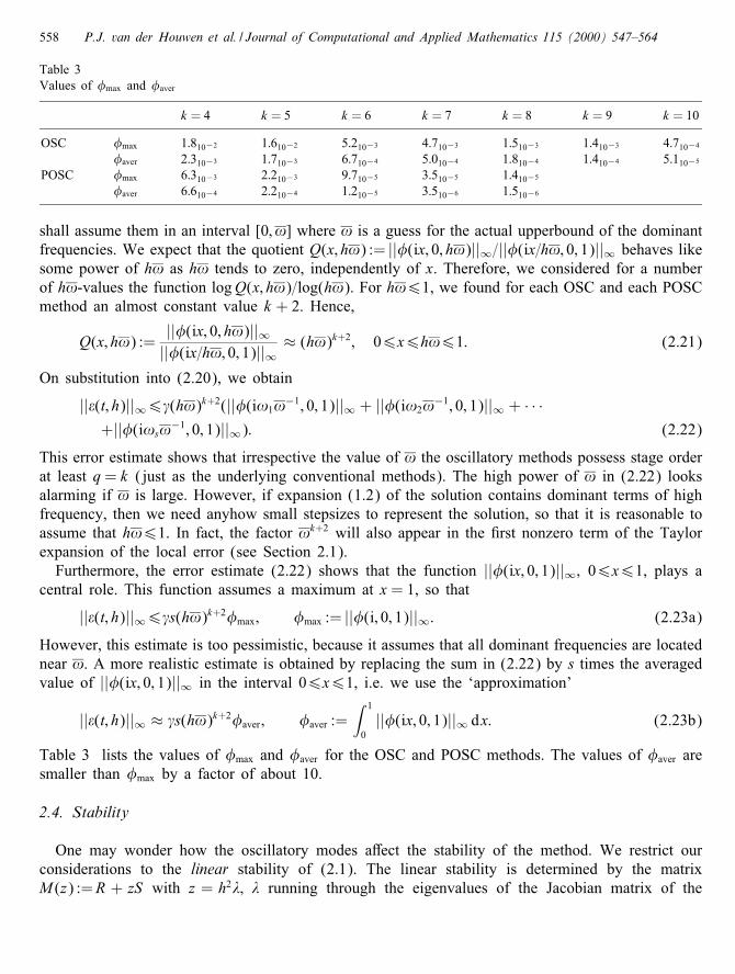
Table 3Values of �max and �aver

k = 4 k = 5 k = 6 k = 7 k = 8 k = 9 k = 10

OSC �max 1:810−2 1:610−2 5:210−3 4:710−3 1:510−3 1:410−3 4:710−4

�aver 2:310−3 1:710−3 6:710−4 5:010−4 1:810−4 1:410−4 5:110−5

POSC �max 6:310−3 2:210−3 9:710−5 3:510−5 1:410−5

�aver 6:610−4 2:210−4 1:210−5 3:510−6 1:510−6

shall assume them in an interval [0; !] where ! is a guess for the actual upperbound of the dominantfrequencies. We expect that the quotient Q(x; h!) := ||�(ix; 0; h!)||∞=||�(ix=h!; 0; 1)||∞ behaves likesome power of h! as h! tends to zero, independently of x. Therefore, we considered for a numberof h!-values the function logQ(x; h!)=log(h!). For h!61, we found for each OSC and each POSCmethod an almost constant value k + 2. Hence,

Q(x; h!) :=||�(ix; 0; h!)||∞||�(ix=h!; 0; 1)||∞ ≈ (h!)k+2; 06x6h!61: (2.21)

On substitution into (2.20), we obtain

||�(t; h)||∞6 (h!)k+2(||�(i!1!−1; 0; 1)||∞ + ||�(i!2!−1; 0; 1)||∞ + · · ·+||�(i!s!−1; 0; 1)||∞): (2.22)

This error estimate shows that irrespective the value of ! the oscillatory methods possess stage orderat least q= k (just as the underlying conventional methods). The high power of ! in (2.22) looksalarming if ! is large. However, if expansion (1.2) of the solution contains dominant terms of highfrequency, then we need anyhow small stepsizes to represent the solution, so that it is reasonable toassume that h!61. In fact, the factor !k+2 will also appear in the �rst nonzero term of the Taylorexpansion of the local error (see Section 2.1).Furthermore, the error estimate (2.22) shows that the function ||�(ix; 0; 1)||∞; 06x61, plays a

central role. This function assumes a maximum at x = 1, so that

||�(t; h)||∞6 s(h!)k+2�max; �max := ||�(i; 0; 1)||∞: (2.23a)

However, this estimate is too pessimistic, because it assumes that all dominant frequencies are locatednear !. A more realistic estimate is obtained by replacing the sum in (2.22) by s times the averagedvalue of ||�(ix; 0; 1)||∞ in the interval 06x61, i.e. we use the ‘approximation’

||�(t; h)||∞ ≈ s(h!)k+2�aver ; �aver :=∫ 1

0||�(ix; 0; 1)||∞ dx: (2.23b)

Table 3 lists the values of �max and �aver for the OSC and POSC methods. The values of �aver aresmaller than �max by a factor of about 10.

2.4. Stability

One may wonder how the oscillatory modes a�ect the stability of the method. We restrict ourconsiderations to the linear stability of (2.1). The linear stability is determined by the matrixM (z) :=R + zS with z = h2�; � running through the eigenvalues of the Jacobian matrix of the


Table 4aStability boundaries for the case != !

h!= h! 0 0.5 1.0 1.5 2.0 2.2 2.3 3.0 3.9 4.0

POSC (6) 0.85 0.87 0.89 0.97 1.18 1.29 0POSC (10) 0.78 0.78 0.78 0.81 0.87 0.89 0.90 1.11 1.45 1.40

Table 4bStability boundaries for the case != 0

h! 0 0.5 1.0 2.0 4.0 6.0 8.0 10.0 11.0 12.0

POSC (6) 0.85 0.86 0.87 0.90 0.98 1.05 1.03 1.10 1.12 0POSC (10) 0.78 0.78 0.78 0.81 0.85 0.91 0.93 0.55

righthand side function f of the ODE (1.1). Assuming that (1.1) is linearly stable itself, we onlyconsider negative values of z. Here, the stability interval is de�ned by the interval −�26z60,where M (z) has its eigenvalues on the unit disk. The value of � is called the stability boundary.As an illustration, we have computed the stability boundaries of the POSC methods with ! = !and with ! = 0. Tables 4a, 4b present values of � for the 6-th order (k = 5) and the 10th-order(k =8) POSC methods (these methods are also used in the numerical experiments in Section 3). Inall cases, the oscillatory approach slightly stabilizes the PSC method until some maximal value ofh! is reached.

3. Numerical experiments

In this section we compare the performance of the OSC and POSC methods in least squares andminimax mode with the nonoscillatory St�ormer–Cowell methods. In the tables of results, we use thefollowing abbreviations:

SC(p) Classical St�ormer–Cowell method (2:6) of order p= k,OSC(p) Oscillatory version of the SC(p) method,PSC(p) Parallel St�ormer–Cowell method {(2.7), Table 1} of order p,POSC(p) Oscillatory version of the PSC(p) method.

If in the examples the exact solutions are known, the starting vector Y0 was taken from thesolution values (y(t0 + bjh)), otherwise it was computed numerically by a one-step method. Weused a few well-known test problems from the literature. The accuracy is de�ned by the numberof correct digits � at the end point (the maximal absolute end point error is written as 10−�). Thenumber of steps taken in the integration interval is denoted by N which is at the same time for allmethods the total number of sequential right-hand sides needed to perform the integration.

3.1. Problems with one dominant frequency

We start with Bessel’s equation [5]

d2ydt2

=−(100 +

14t2

)y; y(1) = J0(10); y′(1) =

12J0(10)− 10J1(10) (3.1)


on the interval [1,10] with exact solution y(t)=√t J0(10t). This equation shows that there is just one

frequency !=√100 + (4t2)−1 ≈ 10. The oscillatory methods were applied with [!;!]= [9:9; 10:1].

The second test problem is the Orbit problem from the Toronto test set [6] on the interval [0,20]with eccentricity � = 0:01. The solution is known to have one dominant frequency ! ≈ 1. Theoscillatory methods were applied with [!;!] = [0:9; 1:1]. The results in Tables 5a, 5b and 6a, 6bindicate that(i) The least-squares approach is unreliable, even for relatively large stepsizes, which is due to the

bad condition of the W matrix.(ii) The minimax approach can be used until the 20 decimals accuracy range.(iii) The minimax approach produces higher accuracies than the conventional approach.The fact that the minimax method is less e�ective in the case of the Orbit problem, particularlyin the high-accuracy range, can be explained by the fact that for high accuracies, frequencies otherthan ! ≈ 1 start to come into play.From now on, we do not apply the least-squares strategy because of its erratic performance.

Table 5a(N; �)-values for the Bessel problem on [1,10]; 6th-order methods with [!;!] = [9:9; 10:1]

Method Version 100 200 400 800

SC(6) Conventional ∗ 2.3 4.0 5.8OSC(6) Least squares 4.7 6.6 8.7 10.6

Minimax 4.7 6.6 8.7 10.6PSC(6) Conventional 1.4 5.9 8.6 9.5POSC(6) Least squares 6.4 8.8 10.9 13.2

Minimax 6.0 8.9 11.0 13.7

Table 5b(N; �)-values for the Bessel problem on [1,10]; 10th-order methods with [!;!] = [9:9; 10:1]


SC(10) Conventional ∗ ∗ 6.7 9.7OSC(10) Least squares ∗ ∗ 8.8 11.1

Minimax ∗ ∗ 12.0 14.7PSC(10) Conventional ∗ 8.3 11.6 15.0POSC(10) Least squares ∗ 10.9 11.2 12.1

Minimax ∗ 13.3 16.5 19.8

Table 6a(N; �)-values for the Orbit problem on [0,20]; 6th-order methods with [!;!] = [0:9; 1:1]

Method Version 40 80 160 320 640

SC(6) Conventional 0.4 2.4 5.0 6.8 8.3OSC(6) Least squares 1.8 3.6 5.1 6.8 8.6

Minimax 1.8 3.6 5.1 6.8 8.6PSC(6) Conventional 2.5 4.7 6.7 8.8 10.9POSC(6) Least squares 3.4 6.1 8.2 10.2 11.5

Minimax 3.4 6.2 8.1 10.1 12.2


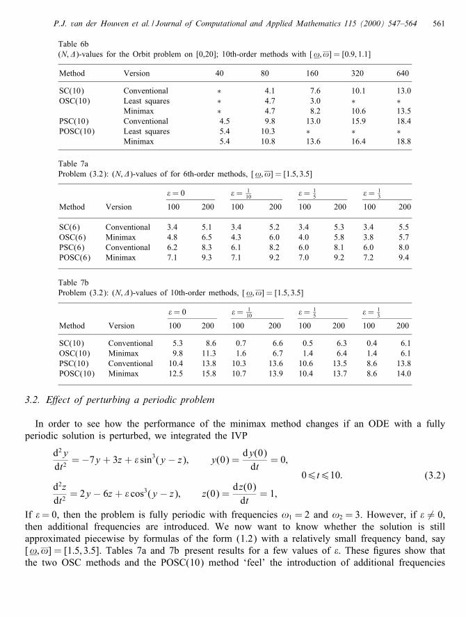
Table 6b(N; �)-values for the Orbit problem on [0,20]; 10th-order methods with [!;!] = [0:9; 1:1]


SC(10) Conventional ∗ 4.1 7.6 10.1 13.0OSC(10) Least squares ∗ 4.7 3.0 ∗ ∗

Minimax ∗ 4.7 8.2 10.6 13.5PSC(10) Conventional 4.5 9.8 13.0 15.9 18.4POSC(10) Least squares 5.4 10.3 ∗ ∗ ∗

Minimax 5.4 10.8 13.6 16.4 18.8

Table 7aProblem (3.2): (N; �)-values of for 6th-order methods, [!;!] = [1:5; 3:5]

� = 0 � = 110 � = 1

5 � = 13

Method Version 100 200 100 200 100 200 100 200

SC(6) Conventional 3.4 5.1 3.4 5.2 3.4 5.3 3.4 5.5OSC(6) Minimax 4.8 6.5 4.3 6.0 4.0 5.8 3.8 5.7PSC(6) Conventional 6.2 8.3 6.1 8.2 6.0 8.1 6.0 8.0POSC(6) Minimax 7.1 9.3 7.1 9.2 7.0 9.2 7.2 9.4

Table 7bProblem (3.2): (N; �)-values of 10th-order methods, [!;!] = [1:5; 3:5]

� = 0 � = 110 � = 1

5 � = 13

Method Version 100 200 100 200 100 200 100 200

SC(10) Conventional 5.3 8.6 0.7 6.6 0.5 6.3 0.4 6.1OSC(10) Minimax 9.8 11.3 1.6 6.7 1.4 6.4 1.4 6.1PSC(10) Conventional 10.4 13.8 10.3 13.6 10.6 13.5 8.6 13.8POSC(10) Minimax 12.5 15.8 10.7 13.9 10.4 13.7 8.6 14.0

3.2. E�ect of perturbing a periodic problem

In order to see how the performance of the minimax method changes if an ODE with a fullyperiodic solution is perturbed, we integrated the IVP

d2ydt2

=−7y + 3z + � sin3(y − z); y(0) =dy(0)dt

= 0;

06t610:d2zdt2

= 2y − 6z + � cos3(y − z); z(0) =dz(0)dt

= 1;

(3.2)

If �= 0, then the problem is fully periodic with frequencies !1 = 2 and !2 = 3. However, if � 6= 0,then additional frequencies are introduced. We now want to know whether the solution is stillapproximated piecewise by formulas of the form (1.2) with a relatively small frequency band, say[!;!] = [1:5; 3:5]. Tables 7a and 7b present results for a few values of �. These �gures show thatthe two OSC methods and the POSC(10) method ‘feel’ the introduction of additional frequencies


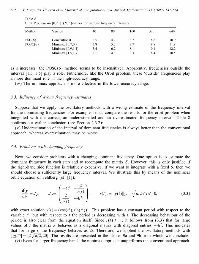
Table 8Orbit Problem on [0,20]: (N; �)-values for various frequency intervals


PSC(6) Conventional 2.5 4.7 6.7 8.8 10.9POSC(6) Minimax [0.7,0.9] 3.8 5.7 7.7 9.8 11.9

Minimax [0.9,1.1] 3.4 6.2 8.1 10.1 12.2Minimax [1.5,1.7] 2.1 4.3 6.3 8.4 10.5

as � increases (the POSC(6) method seems to be insensitive). Apparently, frequencies outside theinterval [1.5, 3.5] play a role. Futhermore, like the Orbit problem, these ‘outside’ frequencies playa more dominant role in the high-accuracy range.(iv) The minimax approach is more e�ective in the lower-accuracy range.

3.3. In uence of wrong frequency estimates

Suppose that we apply the oscillatory methods with a wrong estimate of the frequency intervalfor the dominating frequencies. For example, let us compare the results for the orbit problem whenintegrated with the correct, an underestimated and an overestimated frequency interval. Table 8con�rms our earlier conclusion (see Section 2.3.2):(v) Underestimation of the interval of dominant frequencies is always better than the conventional

approach, whereas overestimation may be worse.

3.4. Problems with changing frequency

Next, we consider problems with a changing dominant frequency. One option is to estimate thedominant frequency in each step and to recompute the matrix S. However, this is only justi�ed ifthe right-hand side function is relatively expensive. If we want to integrate with a �xed S, then weshould choose a su�ciently large frequency interval. We illustrate this by means of the nonlinearorbit equation of Fehlberg (cf. [1]):

d2ydt2

= Jy; J :=

−4t2 − 2

r(t)2r(t)

−4t2

; r(t) := ||y(t)||2;

√�=26t610; (3.3)

with exact solution y(t) = (cos(t2); sin(t2))T. This problem has a constant period with respect to thevariable t2, but with respect to t the period is decreasing with t. The decreasing behaviour of theperiod is also clear from the equation itself. Since r(t) ≈ 1, it follows from (3.3) that for largevalues of t the matrix J behaves as a diagonal matrix with diagonal entries −4t2. This indicatesthat for large t, the frequency behaves as 2t. Therefore, we applied the oscillatory methods with[!;!] = [2

√�=2; 20]. The results are presented in the Tables 9a and 9b from which we conclude:

(vi) Even for larger frequency bands the minimax approach outperforms the conventional approach.


Table 9a(N; �)-values for the Fehlberg problem on [

√�=2; 10]; 6th-order methods with [!;!] = [2

√�=2; 20]

Method Version 160 320 640 1280 2560 5120

SC(6) Conventional ∗ 1.7 3.5 5.3 7.2 9.0OSC(6) Minimax 1.1 3.0 4.7 6.5 8.3 10.1PSC(6) Conventional 2.3 4.2 6.1 8.2 10.3 12.4POSC(6) Minimax 3.6 5.5 7.2 9.2 11.3 13.4

Table 9b(N; �)-values for the Fehlberg problem on [

√�=2; 10]; 10th-order methods with [!;!] = [2

√�=2; 20]


SC(10) Conventional ∗ 3.0 6.0 9.0OSC(10) Minimax ∗ 4.8 7.9 10.7PSC(10) Conventional 4.5 7.6 10.9 14.3POSC(10) Minimax 5.9 9.0 12.3 15.7

3.5. Problems with widely spread dominant frequencies

Finally, we consider the St�ormer problem in polar coordinates on the interval [0,0.5] with u=� asgiven in [3, p. 420 (10.11a)]. Piecewise approximation of the solution by formulas of the form (1.2)leads to quite di�erent intervals of dominant frequencies. Hence, the overall frequency band [!;!]will be quite large, so that we should not expect a better performance of the oscillatory methods.Surprisingly, the results in Tables 10a and 10b show that for quite arbitrary intervals [ !;!] thePOSC methods are at least competitive with the PSC methods. Thus,(vii) Even for problems whose solutions possess widely spread frequencies, the oscillatory methods

do not perform worse than the conventional methods.

Table 10a(N; �)-values for the St�ormer problem on [0; 0:5]; 6th-order methods with various intervals [!;!]


PSC(6) Conventional 0.9 4.6 6.5 8.5 10.5POSC(6) Minimax [0,50] 0.9 4.7 6.6 8.5 10.6

Minimax [0,100] 1.0 5.2 7.1 9.0 11.0Minimax [0,200] 1.6 4.4 6.3 8.3 10.3

Table 10b(N; �)-values for the St�ormer problem on [0; 0:5]; 10th-order methods with various intervals [ !;!]

Method Version 40 80 160

PSC(10) Conventional 0.9 7.0 10.3POSC(10) Minimax [0,50] 1.0 7.1 10.4

Minimax [0,100] 1.0 7.2 10.6Minimax [0,200] 0.8 7.5 10.8


References

[1] E. Fehlberg, Classical Runge–Kutta–Nystr�om formulas with stepsize control for di�erential equations of the formx′′ = f(t; x) (German), Computing 10 (1972) 305–315.

[2] W. Gautschi, Numerical integration of ordinary di�erential equations based on trigonometric polynomials, Numer.Math. 3 (1961) 381–397.

[3] E. Hairer, S.P. NHrsett, G. Wanner, Solving ordinary di�erential equations, Vol. I. Nonsti� problems, Springer, Berlin,1987.

[4] P.J. van der Houwen, E. Messina, J.J.B. de Swart, Parallel St�ormer–Cowell methods for high-precision orbitcomputations, 1998, to appear in Appl. Numer. Math.

[5] P.J. van der Houwen, B.P. Sommeijer, Linear multistep methods with reduced truncation error for periodic initialvalue problems, IMA J. Numer. Anal. 4 (1984) 479–489.

[6] T.E. Hull, W.H. Enright, B.M. Fellen, A.E. Sedgwick, Comparing numerical methods for ordinary di�erentialequations, SIAM J. Numer. Anal. 9 (1972) 603–637.

Oscillatory Störmer–Cowell methods

Documents