Oscillatory Nonautonomous Lucas Sequences

Hindawi Publishing CorporationInternational Journal of Differential EquationsVolume 2010, Article ID 596350, 15 pagesdoi:10.1155/2010/596350

Research ArticleOscillatory Nonautonomous Lucas Sequences

Jose M. Ferreira1 and Sandra Pinelas2

1 Department of Mathematics, Instituto Superior Tecnico, Avenue Rovisco Pais, 1049-001 Lisboa, Portugal2 Department ofMathematics, Universidade dos Acores, R.Mae de Deus, 9500-321 Ponta Delgada, Portugal

Correspondence should be addressed to Sandra Pinelas, [email protected]

Received 18 September 2009; Accepted 3 December 2009

Academic Editor: Elena Braverman

Copyright q 2010 J. M. Ferreira and S. Pinelas. This is an open access article distributed underthe Creative Commons Attribution License, which permits unrestricted use, distribution, andreproduction in any medium, provided the original work is properly cited.

The oscillatory behavior of the solutions of the second-order linear nonautonomous equationx(n + 1) = a(n)x(n) − b(n)x(n − 1), n ∈ N0, where a, b : N0 → R, is studied. Under theassumption that the sequence b(n) dominates somehow a(n), the amplitude of the oscillationsand the asymptotic behavior of its solutions are also analized.

1. Introduction

The aim of this note is to study the oscillatory behavior of the equation

x(n + 1) = a(n)x(n) − b(n)x(n − 1), n ∈ N0, (1.1)

where a, b : N0 → R. Equation (1.1) is the nonautonomous case of the so-called Lucassequences, which are obtained through the recursive law:

x(n + 1) = ax(n) − bx(n − 1), n ∈ N0, (1.2)

which corresponds to have in (1.1) both sequences a(n) and b(n) constant and equal,respectively, to real numbers a and b. Lucas sequences are well known in number theoryas an extension of the Fibonacci sequence (see [1, Chapter 2, Section IV]).

Several particular cases of (1.1) are considered in literature. This is the case of equation(see [2, Chapter 6])

p(n)x(n + 1) + p(n − 1)x(n − 1) = q(n)x(n), n ∈ N0, (1.3)

2 International Journal of Differential Equations

with q(n) being arbitrary and p(n) being positive, corresponding to have in (1.1)

a(n) =q(n)p(n)

, b(n) =p(n − 1)p(n)

. (1.4)

The equation (see [3, 4] and references therein)

Δ2x(n − 1) + P(n)x(n) = 0, n ∈ N0 (1.5)

is also a particular case of (1.1). In fact, (1.5) can be written as

x(n + 1) = (2 − P(n))x(n) − x(n − 1), n ∈ N0, (1.6)

corresponding to have in (1.1), a(n) = 2 − P(n) and b(n) constant and equal to 1. Otherparticular cases of (1.1) will be referred along the text.

As usual, we will say that a solution x(n) of (1.1) is nonoscillatory if it is eithereventually positive or eventually negative. Otherwise x(n) is called oscillatory. When allsolutions of (1.1) are oscillatory, (1.1) is said oscillatory.

It is well known that (1.2) is oscillatory if and only if the polynomial z2 − az+ b has nopositive real roots. This is equivalent to have one of the following two cases:

(i) a ≤ 0, b ≥ 0; (ii) a > 0, b >a2

4. (1.7)

In order to obtain (1.1) oscillatory, this specific case seems to justify that the sequence b(n)be assumed positive. However, for b(n) > 0 for every n, notice that if one has either a(n) ≤ 0eventually or a(n) oscillatory, then x(n) cannot be neither eventually positive nor eventuallynegative. That is, in such circumstances the equation is oscillatory. So hereafter we willassume that a(n) and b(n) are both positive sequences.

Through a direct manipulation of the terms of the solutions of (1.1), we show in thefollowing sections a few results which seem, as far as we know, uncommon in literature. Westate that if b(n) dominates somehow the sequence a(n), then all solutions of the equationexhibit a specific oscillatory and asymptotic behavior. Oscillations through the existence ofperiodic solutions will be studied in a sequel, but they cannot then happen under a similarrelationship between a(n) and b(n).

2. Oscillatory Behavior

The oscillatory behavior of (1.1) can be stated through the application of some results alreadyexistent in literature. This is the case of the following theorem based upon a result in [5].

Theorem 2.1. If

b(n)a(n − 1)a(n)

>14

(2.1)

International Journal of Differential Equations 3

holds eventually and

lim supn→∞

b(n)a(n − 1)a(n)

>14, (2.2)

then (1.1) is oscillatory.

Proof. By making the change of variable

y(n) =2nx(n)

∏n−1k=1a(k)

, (2.3)

one can see that (1.1) is equivalent to

Δ2y(n − 1) =(

1 − 4b(n)a(n − 1)a(n)

)

y(n − 1), n ∈ N0, (2.4)

where by Δ we mean the usual difference operator.Therefore applying [5, Theorem 1.3.1], one can conclude under (2.1) and (2.2) that

every solution of (2.4) is oscillatory. Then, as all terms of the sequence a(n) are positive, alsox(n) is oscillatory.

Remark 2.2. In [6] the equation

x(t) =p∑

j=1

αj(t)x(t − j

), (2.5)

where, for j = 1, . . . , p, αj(t) are real continuous functions on [0,+∞[, is studied. Through [6,Theorem 10], this equation is oscillatory if

βj � αj(t) � γj (2.6)

for j = 1, . . . , p, and

1 =p∑

j=1

γj exp(−λj) (2.7)

has no real roots. Since (1.1) is the discrete case of (2.5) with p = 2, if a(n) and b(n) areboth bounded sequences, one can apply [6, Theorem 10]. As a matter of fact, if a(n) ≤ αand −b(n) ≤ −β, for every n, then through (1.7) one can conclude that (1.1) is oscillatory ifβ > α2/4. This condition implies (2.1) and (2.2).

Remark 2.3. In literature is largely considered the equation

x(n + 1) − x(n) + b(n)x(n − τ) = 0, n ∈ N0, (2.8)


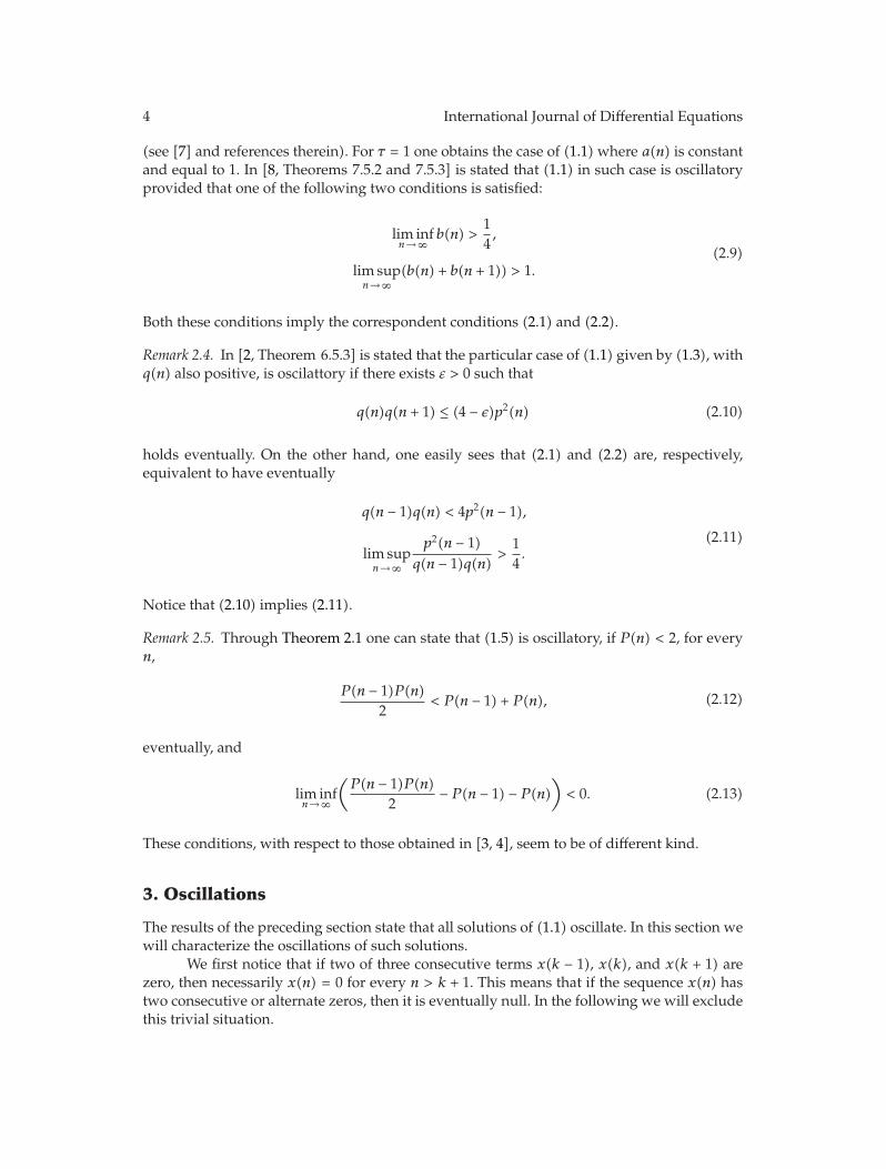
(see [7] and references therein). For τ = 1 one obtains the case of (1.1)where a(n) is constantand equal to 1. In [8, Theorems 7.5.2 and 7.5.3] is stated that (1.1) in such case is oscillatoryprovided that one of the following two conditions is satisfied:

lim infn→∞

b(n) >14,

lim supn→∞

(b(n) + b(n + 1)) > 1.(2.9)

Both these conditions imply the correspondent conditions (2.1) and (2.2).

Remark 2.4. In [2, Theorem 6.5.3] is stated that the particular case of (1.1) given by (1.3), withq(n) also positive, is oscilattory if there exists ε > 0 such that

q(n)q(n + 1) ≤ (4 − ε)p2(n) (2.10)

holds eventually. On the other hand, one easily sees that (2.1) and (2.2) are, respectively,equivalent to have eventually

q(n − 1)q(n) < 4p2(n − 1),

lim supn→∞

p2(n − 1)q(n − 1)q(n)

>14.

(2.11)

Notice that (2.10) implies (2.11).

Remark 2.5. Through Theorem 2.1 one can state that (1.5) is oscillatory, if P(n) < 2, for everyn,

P(n − 1)P(n)2

< P(n − 1) + P(n), (2.12)

eventually, and

lim infn→∞

(P(n − 1)P(n)

2− P(n − 1) − P(n)

)

< 0. (2.13)

These conditions, with respect to those obtained in [3, 4], seem to be of different kind.

3. Oscillations

The results of the preceding section state that all solutions of (1.1) oscillate. In this section wewill characterize the oscillations of such solutions.

We first notice that if two of three consecutive terms x(k − 1), x(k), and x(k + 1) arezero, then necessarily x(n) = 0 for every n > k + 1. This means that if the sequence x(n) hastwo consecutive or alternate zeros, then it is eventually null. In the following we will excludethis trivial situation.


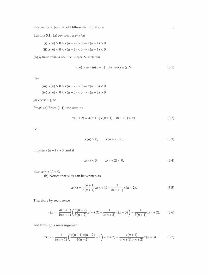
Lemma 3.1. (a) For every n one has

(i) x(n) > 0 ∧ x(n + 2) > 0 ⇒ x(n + 1) > 0,

(ii) x(n) < 0 ∧ x(n + 2) < 0 ⇒ x(n + 1) < 0.

(b) If there exists a positive integerN such that

b(n) > a(n)a(n − 1) for every n ≥ N, (3.1)

then

(iii) x(n) > 0 ∧ x(n + 2) > 0 ⇒ x(n + 3) < 0,

(iv) x(n) < 0 ∧ x(n + 3) < 0 ⇒ x(n + 2) > 0

for every n ≥ N.

Proof. (a) From (1.1) one obtains

x(n + 2) = a(n + 1)x(n + 1) − b(n + 1)x(n). (3.2)

So

x(n) > 0, x(n + 2) > 0 (3.3)

implies x(n + 1) > 0, and if

x(n) < 0, x(n + 2) < 0, (3.4)

then x(n + 1) < 0.(b) Notice that x(n) can be written as

x(n) =a(n + 1)b(n + 1)

x(n + 1) − 1b(n + 1)

x(n + 2). (3.5)

Therefore by recurrence

x(n) =a(n + 1)b(n + 1)

(a(n + 2)b(n + 2)

x(n + 2) − 1b(n + 2)

x(n + 3))

− 1b(n + 1)

x(n + 2), (3.6)

and through a rearrangement

x(n) =1

b(n + 1)

(a(n + 1)a(n + 2)

b(n + 2)− 1

)

x(n + 2) − a(n + 1)b(n + 1)b(n + 2)

x(n + 3). (3.7)


Thus if x(n) > 0, one has

x(n + 3) <(

a(n + 2) − b(n + 2)a(n + 1)

)

x(n + 2), (3.8)

and letting n ≥ N and x(n + 2) > 0 one concludes that x(n + 3) < 0, which shows (iii).Analogously, x(n) < 0 and n ≥ N imply

1b(n + 1)

(

1 − a(n + 1)a(n + 2)b(n + 2)

)

x(n + 2) > − a(n + 1)b(n + 1)b(n + 2)

x(n + 3), (3.9)

and consequently one has x(n + 2) > 0 if x(n + 3) < 0.

We notice that assumption (3.1) implies obviously (2.1) and (2.2), which means thatunder (3.1), equation (1.1) is oscillatory. However, under (3.1) one can further state someinteresting characteristics regarding the oscillations of the solutions of (1.1).

For that purpose, let k ∈ N. Denote by m+k the smallest number of consecutive terms

of x(n), which, for n > k, are positive; by M+k we mean the largest number of consecutive

terms of x(n), which, for n > k, are positive. Analogously, letm−kandM−

kbe, respectively, the

smallest and largest numbers of consecutive terms of x(n), which, for n > k, are negative.

Theorem 3.2. Under (3.1), for every k > N one has m−k,m

+k ≥ 2 and M+

k ,M−k ≤ 3.

Proof. Assuming that there exists a n > k such that

x(n) > 0, x(n + 1) < 0, x(n + 2) > 0, (3.10)

one contradicts (i) of Lemma 3.1. In the same way,

x(n) < 0, x(n + 1) > 0, x(n + 2) < 0 (3.11)

is in contradiction with Lemma 3.1(ii).Moreover if for some n > k one has x(n) = 0, then both x(n + 1) and x(n + 2) are

nonzero real numbers with equal sign and contrary to the sign of x(n − 1) and x(n − 2).Thus m−

k,m+k ≥ 2.

Suppose now that

x(n) > 0, x(n + 1) > 0, x(n + 2) > 0, x(n + 3) > 0. (3.12)

This is a situation which is in contradiction with (iii) of Lemma 3.1.


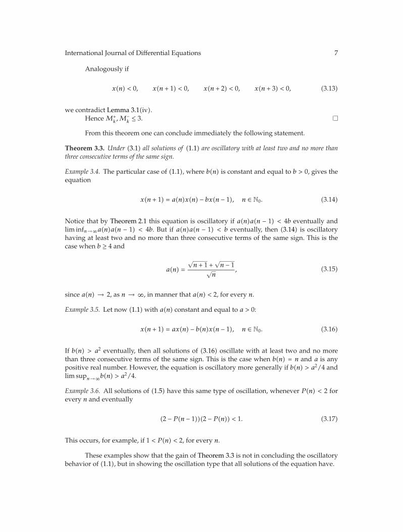
Analogously if

x(n) < 0, x(n + 1) < 0, x(n + 2) < 0, x(n + 3) < 0, (3.13)

we contradict Lemma 3.1(iv).Hence M+

k ,M−k ≤ 3.

From this theorem one can conclude immediately the following statement.

Theorem 3.3. Under (3.1) all solutions of (1.1) are oscillatory with at least two and no more thanthree consecutive terms of the same sign.

Example 3.4. The particular case of (1.1), where b(n) is constant and equal to b > 0, gives theequation

x(n + 1) = a(n)x(n) − bx(n − 1), n ∈ N0. (3.14)

Notice that by Theorem 2.1 this equation is oscillatory if a(n)a(n − 1) < 4b eventually andlim infn→∞a(n)a(n − 1) < 4b. But if a(n)a(n − 1) < b eventually, then (3.14) is oscillatoryhaving at least two and no more than three consecutive terms of the same sign. This is thecase when b ≥ 4 and

a(n) =

√n + 1 +

√n − 1√

n, (3.15)

since a(n) → 2, as n → ∞, in manner that a(n) < 2, for every n.

Example 3.5. Let now (1.1)with a(n) constant and equal to a > 0:

x(n + 1) = ax(n) − b(n)x(n − 1), n ∈ N0. (3.16)

If b(n) > a2 eventually, then all solutions of (3.16) oscillate with at least two and no morethan three consecutive terms of the same sign. This is the case when b(n) = n and a is anypositive real number. However, the equation is oscillatory more generally if b(n) > a2/4 andlim supn→∞b(n) > a2/4.

Example 3.6. All solutions of (1.5) have this same type of oscillation, whenever P(n) < 2 forevery n and eventually

(2 − P(n − 1))(2 − P(n)) < 1. (3.17)

This occurs, for example, if 1 < P(n) < 2, for every n.

These examples show that the gain of Theorem 3.3 is not in concluding the oscillatorybehavior of (1.1), but in showing the oscillation type that all solutions of the equation have.


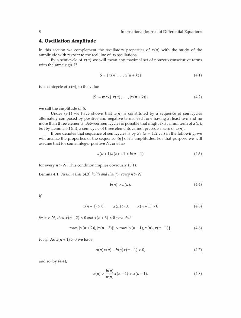
4. Oscillation Amplitude

In this section we complement the oscillatory properties of x(n) with the study of theamplitude with respect to the real line of its oscillations.

By a semicycle of x(n) we will mean any maximal set of nonzero consecutive termswith the same sign. If

S = {x(n), . . . , x(n + k)} (4.1)

is a semicycle of x(n), to the value

|S| = max{|x(n)|, . . . , |x(n + k)|} (4.2)

we call the amplitude of S.Under (3.1) we have shown that x(n) is constituted by a sequence of semicycles

alternately composed by positive and negative terms, each one having at least two and nomore than three elements. Between semicycles is possible that might exist a null term of x(n),but by Lemma 3.1(iii), a semicycle of three elements cannot precede a zero of x(n).

If one denotes that sequence of semicycles is by Sk (k = 1, 2, . . .) in the following, wewill analize the properties of the sequence |Sk| of its amplitudes. For that purpose we willassume that for some integer positive N, one has

a(n + 1)a(n) + 1 < b(n + 1) (4.3)

for every n > N. This condition implies obviously (3.1).

Lemma 4.1. Assume that (4.3) holds and that for every n > N

b(n) > a(n). (4.4)

If

x(n − 1) > 0, x(n) > 0, x(n + 1) > 0 (4.5)

for n > N, then x(n + 2) < 0 and x(n + 3) < 0 such that

max{|x(n + 2)|, |x(n + 3)|} > max{x(n − 1), x(n), x(n + 1)}. (4.6)

Proof. As x(n + 1) > 0 we have

a(n)x(n) − b(n)x(n − 1) > 0, (4.7)

and so, by (4.4),

x(n) >b(n)a(n)

x(n − 1) > x(n − 1). (4.8)


Now we will prove that −x(n + 2) > x(n) and −x(n + 3) > x(n + 1). In fact, we have

x(n + 2) = a(n + 1)x(n + 1) − b(n + 1)x(n)

= a(n + 1)(a(n)x(n) − b(n)x(n − 1)) − b(n + 1)x(n)

= (a(n + 1)a(n) − b(n + 1))x(n) − a(n + 1)b(n)x(n − 1)

< (a(n + 1)a(n) − b(n + 1))x(n)

(4.9)

and by (4.3) we obtain

x(n + 2) < −x(n), (4.10)

for every n > N.In the same way one can conclude that

x(n + 3) < (a(n + 2)a(n + 1) − b(n + 2))x(n + 1) < −x(n + 1). (4.11)

This proves the lemma.

Lemma 4.2. Assume that (4.3) holds and that for every n > N

a(n + 1)b(n) > 1. (4.12)

If

x(n − 1) > 0, x(n) > 0, x(n + 1) < 0, x(n + 2) < 0 (4.13)

for n > N, then

max{|x(n + 1)|, |x(n + 2)|} > max{x(n − 1), x(n)}. (4.14)

Proof. Noticing that

x(n + 2) = a(n + 1)(a(n)x(n) − b(n)x(n − 1)) − b(n + 1)x(n)

= (a(n + 1)a(n) − b(n + 1))x(n) − a(n + 1)b(n)x(n − 1),(4.15)

by (4.3) one has

x(n + 2) < (a(n + 1)a(n) − b(n + 1))x(n) < −x(n),x(n + 2) < −a(n + 1)b(n)x(n − 1) < −x(n − 1),

(4.16)

which proves the lemma.


Lemma 4.3. Assume that (4.3), (4.4), and (4.12) hold. If

x(n − 1) > 0, x(n) > 0, x(n + 1) = 0, x(n + 2) < 0, x(n + 3) < 0 (4.17)

for n > N, then

max{|x(n + 2)|, |x(n + 3)|} > max{x(n − 1), x(n)}. (4.18)

Proof. First take into account that x(n + 1) = 0 implies

a(n)x(n) = b(n)x(n − 1) ⇐⇒ x(n) =b(n)a(n)

x(n − 1) > x(n − 1). (4.19)

Notice now that

x(n + 2) = −b(n + 1)x(n) < −x(n) (4.20)

since (4.3) implies b(n) > 1 for every n > N. On the other hand

x(n + 3) = a(n + 2)x(n + 2)

= −a(n + 2)b(n + 1)x(n)

< −x(n).(4.21)

This achieves the proof.

Remark 4.4. Observe that u(n) = −x(n) is also a solution of (1.1)which of course has the sameoscillatory characteristics as x(n). This fact enables to conclude similar lemmas by simplechange of sign.

Theorem 4.5. Assuming that (4.3), (4.4), and (4.12) hold, then |Sk| is eventually increasing.

Proof. Let Sk and Sk+1 be two consecutive semicycles. Several cases can be performed.(1) Assume that

Sk = {x(n − 1) > 0, x(n) > 0, x(n + 1) > 0},Sk+1 = {x(n + 2) < 0, x(n + 3) < 0}.

(4.22)

Then by Lemma 4.1 one has |Sk+1| > |Sk|.By Remark 4.4 the same holds if

Sk = {x(n − 1) < 0, x(n) < 0, x(n + 1) < 0},Sk+1 = {x(n + 2) > 0, x(n + 3) > 0}.

(4.23)


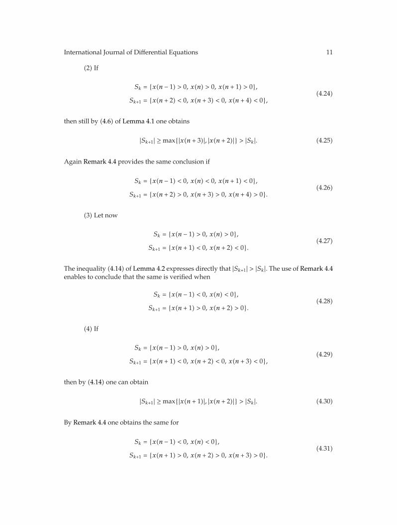
(2) If

Sk = {x(n − 1) > 0, x(n) > 0, x(n + 1) > 0},Sk+1 = {x(n + 2) < 0, x(n + 3) < 0, x(n + 4) < 0},

(4.24)

then still by (4.6) of Lemma 4.1 one obtains

|Sk+1| ≥ max{|x(n + 3)|, |x(n + 2)|} > |Sk|. (4.25)

Again Remark 4.4 provides the same conclusion if

Sk = {x(n − 1) < 0, x(n) < 0, x(n + 1) < 0},Sk+1 = {x(n + 2) > 0, x(n + 3) > 0, x(n + 4) > 0}.

(4.26)

(3) Let now

Sk = {x(n − 1) > 0, x(n) > 0},Sk+1 = {x(n + 1) < 0, x(n + 2) < 0}.

(4.27)

The inequality (4.14) of Lemma 4.2 expresses directly that |Sk+1| > |Sk|. The use of Remark 4.4enables to conclude that the same is verified when

Sk = {x(n − 1) < 0, x(n) < 0},Sk+1 = {x(n + 1) > 0, x(n + 2) > 0}.

(4.28)

(4) If

Sk = {x(n − 1) > 0, x(n) > 0},Sk+1 = {x(n + 1) < 0, x(n + 2) < 0, x(n + 3) < 0},

(4.29)

then by (4.14) one can obtain

|Sk+1| ≥ max{|x(n + 1)|, |x(n + 2)|} > |Sk|. (4.30)

By Remark 4.4 one obtains the same for

Sk = {x(n − 1) < 0, x(n) < 0},Sk+1 = {x(n + 1) > 0, x(n + 2) > 0, x(n + 3) > 0}.

(4.31)


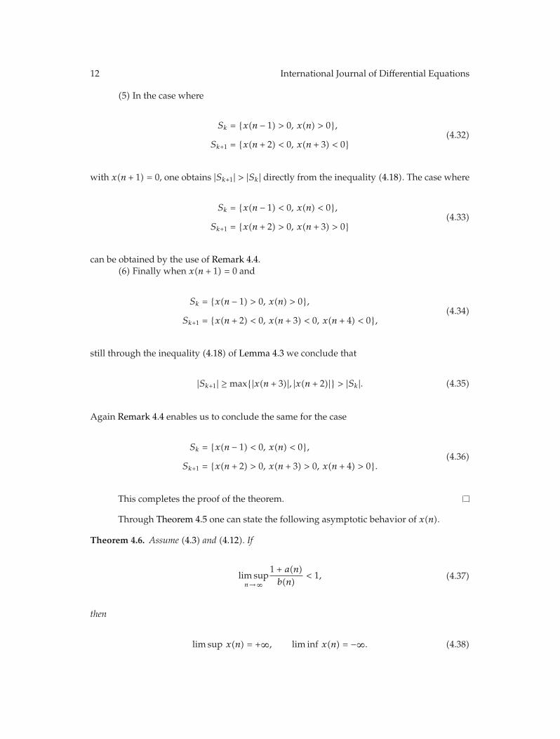
(5) In the case where

Sk = {x(n − 1) > 0, x(n) > 0},Sk+1 = {x(n + 2) < 0, x(n + 3) < 0}

(4.32)

with x(n + 1) = 0, one obtains |Sk+1| > |Sk| directly from the inequality (4.18). The case where

Sk = {x(n − 1) < 0, x(n) < 0},Sk+1 = {x(n + 2) > 0, x(n + 3) > 0}

(4.33)

can be obtained by the use of Remark 4.4.(6) Finally when x(n + 1) = 0 and

Sk = {x(n − 1) > 0, x(n) > 0},Sk+1 = {x(n + 2) < 0, x(n + 3) < 0, x(n + 4) < 0},

(4.34)

still through the inequality (4.18) of Lemma 4.3 we conclude that

|Sk+1| ≥ max{|x(n + 3)|, |x(n + 2)|} > |Sk|. (4.35)

Again Remark 4.4 enables us to conclude the same for the case

Sk = {x(n − 1) < 0, x(n) < 0},Sk+1 = {x(n + 2) > 0, x(n + 3) > 0, x(n + 4) > 0}.

(4.36)

This completes the proof of the theorem.

Through Theorem 4.5 one can state the following asymptotic behavior of x(n).

Theorem 4.6. Assume (4.3) and (4.12). If

lim supn→∞

1 + a(n)b(n)

< 1, (4.37)

then

lim sup x(n) = +∞, lim inf x(n) = −∞. (4.38)


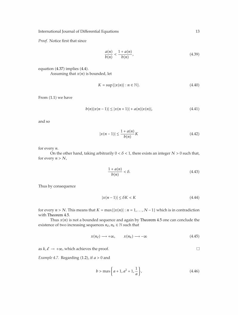
Proof. Notice first that since

a(n)b(n)

<1 + a(n)b(n)

, (4.39)

equation (4.37) implies (4.4).Assuming that x(n) is bounded, let

K = sup{|x(n)| : n ∈ N}. (4.40)

From (1.1)we have

b(n)|x(n − 1)| ≤ |x(n + 1)| + a(n)|x(n)|, (4.41)

and so

|x(n − 1)| ≤ 1 + a(n)b(n)

K (4.42)

for every n.On the other hand, taking arbitrarily 0 < δ < 1, there exists an integerN > 0 such that,

for every n > N,

1 + a(n)b(n)

< δ. (4.43)

Thus by consequence

|x(n − 1)| ≤ δK < K (4.44)

for every n > N. This means thatK = max{|x(n)| : n = 1, . . . ,N − 1}which is in contradictionwith Theorem 4.5.

Thus x(n) is not a bounded sequence and again by Theorem 4.5 one can conclude theexistence of two increasing sequences n, nk ∈ N such that

x(n) −→ +∞, x(nk) −→ −∞ (4.45)

as k, → +∞, which achieves the proof.

Example 4.7. Regarding (1.2), if a > 0 and

b > max{

a + 1, a2 + 1,1a

}

, (4.46)


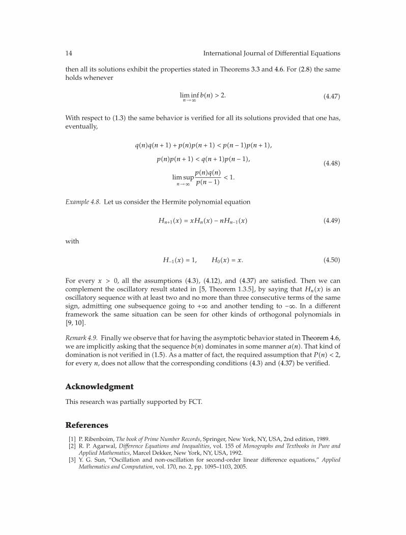
then all its solutions exhibit the properties stated in Theorems 3.3 and 4.6. For (2.8) the sameholds whenever

lim infn→∞

b(n) > 2. (4.47)

With respect to (1.3) the same behavior is verified for all its solutions provided that one has,eventually,

q(n)q(n + 1) + p(n)p(n + 1) < p(n − 1)p(n + 1),

p(n)p(n + 1) < q(n + 1)p(n − 1),

lim supn→∞

p(n)q(n)p(n − 1)

< 1.

(4.48)

Example 4.8. Let us consider the Hermite polynomial equation

Hn+1(x) = xHn(x) − nHn−1(x) (4.49)

with

H−1(x) = 1, H0(x) = x. (4.50)

For every x > 0, all the assumptions (4.3), (4.12), and (4.37) are satisfied. Then we cancomplement the oscillatory result stated in [5, Theorem 1.3.5], by saying that Hn(x) is anoscillatory sequence with at least two and no more than three consecutive terms of the samesign, admitting one subsequence going to +∞ and another tending to −∞. In a differentframework the same situation can be seen for other kinds of orthogonal polynomials in[9, 10].

Remark 4.9. Finally we observe that for having the asymptotic behavior stated in Theorem 4.6,we are implicitly asking that the sequence b(n) dominates in some manner a(n). That kind ofdomination is not verified in (1.5). As a matter of fact, the required assumption that P(n) < 2,for every n, does not allow that the corresponding conditions (4.3) and (4.37) be verified.

Acknowledgment

This research was partially supported by FCT.

References

[1] P. Ribenboim, The book of Prime Number Records, Springer, New York, NY, USA, 2nd edition, 1989.[2] R. P. Agarwal, Difference Equations and Inequalities, vol. 155 of Monographs and Textbooks in Pure and

Applied Mathematics, Marcel Dekker, New York, NY, USA, 1992.[3] Y. G. Sun, “Oscillation and non-oscillation for second-order linear difference equations,” Applied

Mathematics and Computation, vol. 170, no. 2, pp. 1095–1103, 2005.


[4] Y. Zhou, B. G. Zhang, and C. F. Li, “Remarks on oscillation and nonoscillation for second-order lineardifference equations,” Applied Mathematics Letters, vol. 21, no. 6, pp. 578–580, 2008.

[5] R. P. Agarwal, S. Grace, and D. O’Regan, Oscillation Theory for Difference and Functional DifferentialEquations, Kluwer Academic Publishers, Dordrecht, The Netherlands, 2000.

[6] J. M. Ferreira and A. M. Pedro, “Oscillations of delay difference systems,” Journal of MathematicalAnalysis and Applications, vol. 221, no. 1, pp. 364–383, 1998.

[7] G. E. Chatzarakis and I. P. Stavroulakis, “Oscillations of first order linear delay difference equations,”The Australian Journal of Mathematical Analysis and Applications, vol. 3, no. 1, article 14, pp. 1–11, 2006.

[8] I. Gyori and G. Ladas, Oscillation Theory of Delay Differential Equations, Oxford MathematicalMonographs, Oxford University Press, New York, NY, USA, 1991.

[9] J. M. Ferreira, S. Pinelas, and A. Ruffing, “Nonautonomous oscillators and coefficient evaluation fororthogonal function systems,” Journal of Difference Equations and Applications, vol. 15, no. 11-12, pp.1117–1133, 2009.

[10] J. M. Ferreira, S. Pinelas, and A. Ruffing, “Oscillatory difference equations and moment problems,”to appear in International Journal of Difference Equations.

Submit your manuscripts athttp://www.hindawi.com

Hindawi Publishing Corporationhttp://www.hindawi.com Volume 2014

MathematicsJournal of


Mathematical Problems in Engineering

Hindawi Publishing Corporationhttp://www.hindawi.com

Differential EquationsInternational Journal of

Volume 2014

Applied MathematicsJournal of


Probability and StatisticsHindawi Publishing Corporationhttp://www.hindawi.com Volume 2014

Journal of


Mathematical PhysicsAdvances in

Complex AnalysisJournal of


OptimizationJournal of


CombinatoricsHindawi Publishing Corporationhttp://www.hindawi.com Volume 2014

International Journal of


Operations ResearchAdvances in

Journal of


Function Spaces

Abstract and Applied AnalysisHindawi Publishing Corporationhttp://www.hindawi.com Volume 2014

International Journal of Mathematics and Mathematical Sciences


The Scientific World JournalHindawi Publishing Corporation http://www.hindawi.com Volume 2014


Algebra

Discrete Dynamics in Nature and Society



Decision SciencesAdvances in

Discrete MathematicsJournal of

Hindawi Publishing Corporationhttp://www.hindawi.com

Volume 2014 Hindawi Publishing Corporationhttp://www.hindawi.com Volume 2014

Stochastic AnalysisInternational Journal of

Oscillatory Nonautonomous Lucas Sequences

Documents