Design Concept for an Automotive Control Arm - OS-2010 This tutorial uses OptiStruct's topology optimization functionality to create a design concept for an automotive control arm required to meet performance specifications. The finite element mesh containing designable (blue) and non-designable regions (yellow) is shown in the figure below. Part specifications constrain the resultant displacement of the point where loading is applied for three load cases to 0.05mm, 0.02mm, and 0.04mm, respectively . The optimal design would use as little material as possible. Finite element mesh containing designable (blue) and non-designable (yellow) material. A finite element model representing the designable and non-designable material (shown in f igure) is imported into HyperMesh. Appropriate properties, boundary conditions, loads, and optimization parameters are defined and the OptiStruct software is used to determine the optimal material distribution. The results (the material layout) are viewed as contours of a normalized density value ranging from 0.0 to 1.0 in the design space. Isosurfaces are also used to view the density results. Areas that need reinforcement will tend towards a density of 1.0. The optimization problem for this tutorial is stated as: Objective: Minimize volume. Constraints: SUBCASE 1 - The resulta nt displacemen t of the poi nt wh ere loading is applied must be less than 0.05mm. SUBCASE 2 - The resultant displacement of the poi nt where loading is applied must be less than 0.02mm. SUBCASE 3 - The resulta nt displacemen t of the poi nt wh ere loading is applied must be less than 0.04mm. Design variables: Microstructural void sizes and orientations in the design space. The following exercises are included: • Setting up the FE model in HyperMesh • Setting up the optimization in HyperMesh • Post-processing the results in HyperView Exercise Setting Up the FE Model in HyperMesh Step 1: Launch HyperMesh, Set the User Profile and Retrieve the File RADIOSS , MotionS olve, a nd OptiS truct T utoria ls > OptiStr uct > T opolo.. . file:/// C:/Altair/ hw10.1 /help/h wsolve rs/os2 010.ht m?zoo m_highl ightsub ... 1 of 12 9/27/2011 5:16 PM

Welcome message from author
This document is posted to help you gain knowledge. Please leave a comment to let me know what you think about it! Share it to your friends and learn new things together.
Transcript

7/29/2019 OS-2010 Design Concept for an Automotive Control Arm
http://slidepdf.com/reader/full/os-2010-design-concept-for-an-automotive-control-arm 1/12
Design Concept for an Automotive Control Arm - OS-2010
This tutorial uses OptiStruct's topology optimization functionality to create a design concept for an automotive control
arm required to meet performance specifications. The finite element mesh containing designable (blue) and
non-designable regions (yellow) is shown in the figure below. Part specifications constrain the resultant displacement
of the point where loading is applied for three load cases to 0.05mm, 0.02mm, and 0.04mm, respectively. The optimaldesign would use as little material as possible.
Finite element mesh containing designable (blue) and non-designable (yellow) material.
A finite element model representing the designable and non-designable material (shown in figure) is imported into
HyperMesh. Appropriate properties, boundary conditions, loads, and optimization parameters are defined and the
OptiStruct software is used to determine the optimal material distribution. The results (the material layout) are viewed
as contours of a normalized density value ranging from 0.0 to 1.0 in the design space. Isosurfaces are also used to
view the density results. Areas that need reinforcement will tend towards a density of 1.0.
The optimization problem for this tutorial is stated as:
Objective: Minimize volume.
Constraints: SUBCASE 1 - The resultant displacement of the point where loading is
applied must be less than 0.05mm.
SUBCASE 2 - The resultant displacement of the point where loading is
applied must be less than 0.02mm.
SUBCASE 3 - The resultant displacement of the point where loading is
applied must be less than 0.04mm.
Design variables: Microstructural void sizes and orientations in the design space.
The following exercises are included:
• Setting up the FE model in HyperMesh
• Setting up the optimization in HyperMesh
• Post-processing the results in HyperView
Exercise
Setting Up the FE Model in HyperMesh
Step 1: Launch HyperMesh, Set the User Profile and Retrieve the File
IOSS, MotionSolve, and OptiStruct Tutorials > OptiStruct > Topolo... file:///C:/Altair/hw10.1/help/hwsolvers/os2010.htm?zoom_high
2 9/27/2011

7/29/2019 OS-2010 Design Concept for an Automotive Control Arm
http://slidepdf.com/reader/full/os-2010-design-concept-for-an-automotive-control-arm 2/12
1. Launch HyperMesh
2. Choose the OptiStruct User Profile and click OK .
This loads the user profile. It includes the appropriate template, macro menu, and import reader, paring down the
functionality of HyperMesh to what is relevant for generating models in Bulk Data Format for RADIOSS and
OptiStruct. The User Profiles GUI can also be accessed from the Preferences pull-down menu on the toolbar.
3. From the File pull-down menu on the toolbar, select Open.
4. Select the carm.hm file, located in the HyperWorks installation directory under
<install_directory>/tutorials/hwsolvers/optistruct/ .
5. Click Open.
Step 2: Create Materials and Properties and Assign to Proper Components
1. Click Model tab on the tab menu.
2. Right click inside the Model Browser window and move the cursor over Create to activate the extended menu and
select Material .
3. In the Name: field, type Steel.
4. For Card image:, choose MAT1 as the material type.
5. Click on Create/Edit .
The MAT1 card image pops up.
6. For E , enter the value 2.0E5.
7. For Nu , enter the value 0.3.
8. Click return.
9. Right click inside the Model Browser window and move the cursor over Create to activate the extended menu and
select Property .
10. In the Name: field, type design_prop.
11. For Card image:, choose PSOLID as the property type.
12. Set Material: as Steel .
13. Click on Create.
14. Right click inside the Model Browser window and move the cursor over Create to activate the extended menu and
select Property .
15. In the Name: field, type nondesign_prop.
16. For Card image:, choose PSOLID as the property type.
17. Set Material: as Steel .
18. Click on Create.
19. From the Collectors pull down menu, move the cursor over Assign to activate the extended menu and select
Components Property .
20. Click on comps, check the nondesign box, and then click select .
21. Click on property = and select nondesign_prop.
22. Click on assign.
23. Repeat steps 22 – 22 to assign design_prop to the design component.
24. Click return.
IOSS, MotionSolve, and OptiStruct Tutorials > OptiStruct > Topolo... file:///C:/Altair/hw10.1/help/hwsolvers/os2010.htm?zoom_high
2 9/27/2011

7/29/2019 OS-2010 Design Concept for an Automotive Control Arm
http://slidepdf.com/reader/full/os-2010-design-concept-for-an-automotive-control-arm 3/12
Step 3: Create Load Collectors
Next we will create four load collectors (SPC, Brake, Corner and Pothole) and assign each a color. Follow these steps
for each load collector.
1. Right click inside the Model Browser window and move the cursor over Create to activate the extended menu and
select LoadCollector .
2. In the Name: field, type SPC.
When in this popup, do not hit the Enter key on the keyboard until you are completely done.
3. Leave the Card image: field set to None.
4. Select a suitable color.
5. Click on Create.
6. Similarly, create load collectors called Brake, Corner , and Pothole.
Step 4: Apply Constraints
We need to create constraints and assign them to the SPC load collector as outlined in the following steps.
1. From Model Browser, expand LoadCollectors, right click on SPC , and click on Make Current .
2. From the Analysis page, enter the constraints panel.
3. Make sure the create subpanel is selected using the radio buttons on the left-hand side of the panel.
4. Select the node at one end of the bushing (see the figure below) by clicking on it in the graphics window.
5. Constrain dof1, dof2, and dof3; make sure dofs 1, 2, and 3 are checked and dofs 4, 5, and 6 are unchecked.
Dofs with a check will be constrained while dofs without a check will be free.
Dofs 1, 2, and 3 are x, y, and z translation degrees of freedom.
Dofs 4, 5, and 6 are x, y, and z rotational degrees of freedom.
6. Click create.
A constraint is created. A constraint symbol (triangle) appears in the graphics window at the selected node. Thenumber 123 is written beside the constraint symbol, indicating that dof1, dof2 and dof3 are constrained.
Constraining dof1, dof2 and dof3 at one end of the bushing.
7. Select the node at the other end of the bushing (see the following figure) by clicking on it in the graphics window.
8. Constrain dof2 and dof3; make sure dofs 2 and 3 are checked.
9. Click create.
A constraint is created. A constraint symbol (triangle) appears in the graphics window at the selected node. The
number 23 is written beside the constraint symbol, indicating that dof2 and dof3 are constrained.
IOSS, MotionSolve, and OptiStruct Tutorials > OptiStruct > Topolo... file:///C:/Altair/hw10.1/help/hwsolvers/os2010.htm?zoom_high
2 9/27/2011

7/29/2019 OS-2010 Design Concept for an Automotive Control Arm
http://slidepdf.com/reader/full/os-2010-design-concept-for-an-automotive-control-arm 4/12
Constraining dof2 and dof3 at the other end of the bushing.
10. Click nodes and select by id from the extended entity selection window.
11. Type the value 3239 and press Enter key.
12. This selects node ID 3239 (see the next figure).
13. Constrain only dof3.
14. Click create.
A constraint is created. A constraint symbol (triangle) appears in the graphics window at the selected node. Thenumber 3 is written beside the constraint symbol, indicating that dof3 is constrained.
Constraining dof3 on node ID 3239.
15. Click return to go to the main menu.
Step 5: Apply Forces for Brake, Corner, and Pothole Loadcases
1. From the Model Browser , expand LoadCollectors, right click on Brake, and click on Make Current .
2. From Analysis page, select forces panel.
3. Click nodes and select by id from the extended entity selection menu.
4. Type the node number 2699 and press the Enter key.
5. Click magnitude=, enter 1000.0 and press the Enter key.
6. Set the switch below to x-axis.
IOSS, MotionSolve, and OptiStruct Tutorials > OptiStruct > Topolo... file:///C:/Altair/hw10.1/help/hwsolvers/os2010.htm?zoom_high
2 9/27/2011

7/29/2019 OS-2010 Design Concept for an Automotive Control Arm
http://slidepdf.com/reader/full/os-2010-design-concept-for-an-automotive-control-arm 5/12
7. Click create.
An arrow, pointing the x direction, should appear at the node on the screen.
8. For better visualization of the arrows, select uniform size=, type 100, and press Enter .
9. From the Model Browser , under the expanded LoadCollectors, right click on Corner , and click on Make Current .
10. Click nodes and select by id from the extended entity selection menu.
11. Type the node number 2699 and press Enter .
12. Click magnitude=, enter 1000.0, and press Enter .
13. Set the switch below to y-axis.
14. Click create.
An arrow pointing in the Y direction should appear at the node on the screen.
15. From the Model Browser , under the expanded LoadCollectors, right click on Pothole, and click Make Current .
16. Click nodes and select by id from the extended entity selection menu.
17. Type the node number 2699 and press Enter .
18. Click magnitude=, enter 1000.0, and press Enter .
19. Set the switch below to z-axis.
20. Click create.
An arrow, pointing in the Z direction, should appear at the node on the screen.
21. Click return to go back to the Analysis page.
Three separate forces in load collectors: brake, corner, and pothole with the component "design" turned off using the display panel.
Step 6: Create Brake, Corner & Pothole Loadcases
The last step in establishing boundary conditions is the creation of a subcase.
1. From the Analysis page enter the loadsteps panel.
2. Click name=, enter Brake, and press Enter .
3. Select type as linear static .
4. Check the box preceding SPC .
An entry field appears to the right of SPC .
IOSS, MotionSolve, and OptiStruct Tutorials > OptiStruct > Topolo... file:///C:/Altair/hw10.1/help/hwsolvers/os2010.htm?zoom_high
2 9/27/2011

7/29/2019 OS-2010 Design Concept for an Automotive Control Arm
http://slidepdf.com/reader/full/os-2010-design-concept-for-an-automotive-control-arm 6/12
5. Click on the entry field and select SPC from the list of load collectors.
6. Check the box preceding Load and select Brake from the list of load collectors.
7. Click Create.
8. Similarly create the load cases Corner [by selecting the load collectors Corner and SPC ] and Pothole [by
selecting the load collectors Pothole and SPC ].
9. Click return to go back to the Analysis page.
Setting Up the Optimization in HyperMesh
Step 7: Define the Topology Design Variables
1. From the Analysis page enter the optimization panel.
2. Enter the topology panel.
3. Make sure the create subpanel is selected using the radio buttons on the left-hand side of the panel.
4. Click DESVAR=, type design_prop, and press Enter .
5. Click props , choose design_prop from the list of props, and click on select .
6. Choose type: PSOLID.
7. Click Create.
A topology design space definition, design_prop, has been created. All elements organized in this design property
collector are now included in the design space.
8. Click return to go back to the optimization panel.
Step 8: Create a Volume and Displacement Response
1. Enter the responses panel.
2. Click response = and enter vol.
3. Click on the response type switch and select volume from the pop-up menu.
4. Ensure the regional selection is set to total (this is the default).
5. Click create.
A response, vol, is defined for the total volume of the model.
6. Click response = and enter disp1.
7. Click on the response type switch and select static displacement from the pop-up menu.
8. Click nodes and select by ID from the extended entity selection menu that pops up.
9. Type 2699 and hit Enter .
The node where the three forces are applied is selected.
10. Select total disp from the radio options.
This is the vector sum of the x, y, and z translations.
11. Click create.
A response, disp1, is defined for the total displacement of node 2699.
12. Click return to go back to the optimization panel.
IOSS, MotionSolve, and OptiStruct Tutorials > OptiStruct > Topolo... file:///C:/Altair/hw10.1/help/hwsolvers/os2010.htm?zoom_high
2 9/27/2011

7/29/2019 OS-2010 Design Concept for an Automotive Control Arm
http://slidepdf.com/reader/full/os-2010-design-concept-for-an-automotive-control-arm 7/12
Step 9: Define the Objective
1. Enter the objective panel.
2. The switch on the left should be set to min.
3. Click response= and select Vol .
4. Click create.
5. Click return to exit the optimization panel.
Step 10: Create Constraints on Displacement Responses
In this step we set the upper and lower bound constraint criteria for this analysis.
1. Enter the dconstraints panel.
2. Click constraint= and enter constr1.
3. Check the box for upper bound only.
4. Click upper bound= and enter 0.05.
5. Select response= and set it to disp1.
6. Click loadsteps.
7. Check the box next to Brake.
8. Click select .
9. Click create.
10. Click constraint= and enter constr2.
11. Check the box for upper bound only.
12. Click upper bound= and enter 0.02.
13. Select response= and set it to Corner .
14. Click create.
15. Click constraint= and enter constr3.
16. Check the box for upper bound only.
17. Click upper bound= and enter 0.04.
18. Select response= and set it to Pothole.
19. Click create.
20. Click return twice to return to the main menu.
Step 11: Check the Optimization Problem A check run may be performed in which OptiStruct will estimate the amount of RAM and disk space required to run the
model. During the check run, OptiStruct will also scan the deck checking that all the necessary information required to
perform an analysis or optimization is present and also that this information is not conflicting.
1. From the Analysis page enter the OptiStruct panel.
2. Click save as following the input file: field
3. Select the directory where you would like to write the OptiStruct model file and enter the name for the model,
carm_check.fem, in the File name: field.
The .fem extension is for OptiStruct input decks.
IOSS, MotionSolve, and OptiStruct Tutorials > OptiStruct > Topolo... file:///C:/Altair/hw10.1/help/hwsolvers/os2010.htm?zoom_high
2 9/27/2011

7/29/2019 OS-2010 Design Concept for an Automotive Control Arm
http://slidepdf.com/reader/full/os-2010-design-concept-for-an-automotive-control-arm 8/12
4. Click Save.
5. Note the name and location of the carm_check.fem file displays in the input file: field.
6. Set the export options: toggle to all .
7. Click the run options: switch and select check .
8. Set the memory options: toggle to memory default .
9. Click OptiStruct .
This launches the OptiStruct check run.
Once the processing is complete (indicated in the UNIX or MSDOS window which pops up), view the file
carm_check.out. This is the OptiStruct output file containing specific information on the file setup, optimization
problem setup, RAM and disk space requirement for the run. Review this file for possible warnings and errors.
Is the optimization problem set up correctly? See Optimization Problem Parameters section of the
carm_check.out file.
The objective function? See Optimization Problem Parameters section of the carm_check.out file.
The constraints? See Optimization Problem Parameters section of the carm_check.out file.
What is the recommended amount of RAM for an In-Core solution? See Memory Estimation Information section of
thecarm_check.out
file.
Is there enough disk space to run the optimization? See Disk Space Estimation Information section of the
carm_check.out file.
Step 12: Run the Optimization Problem
1. From the Analysis page enter the OptiStruct panel.
2. Click save as, enter carm_complete.fem as the file name, and click Save.
3. Click the run options: switch and select optimization.
4. Click OptiStruct to run the optimization.
The message Processing complete appears in the window at the completion of the job. OptiStruct also reports
error messages if any exist. The file carm_complete.out can be opened in a text editor to find details regarding
any errors. This file is written to the same directory as the .fem file.
5. Close the DOS window or shell and click return.
The default files written to the directory are:
carm_complete.hgdata HyperGraph file containing data for the objective function,
percent constraint violations, and constraint for each
iteration.
carm_complete.his_data OptiStruct history file containing iteration number,
objective function values and percent of constraint
violation for each iteration.
carm_complete.HM.comp.cmf HyperMesh command file used to organize elements into
components based on their density result values. This
file is only used with OptiStruct topology optimization
runs.
carm_complete.HM.ent.cmf HyperMesh command file used to organize elements into
entity sets based on their density result values. This file
is only used with OptiStruct topology optimization runs.
IOSS, MotionSolve, and OptiStruct Tutorials > OptiStruct > Topolo... file:///C:/Altair/hw10.1/help/hwsolvers/os2010.htm?zoom_high
2 9/27/2011

7/29/2019 OS-2010 Design Concept for an Automotive Control Arm
http://slidepdf.com/reader/full/os-2010-design-concept-for-an-automotive-control-arm 9/12
carm_complete.html HTML report of the optimization, giving a summary of the
problem formulation and the results from the final
iteration.
carm_complete.oss OSSmooth file with a default density threshold of 0.3.
The user may edit the parameters in the file to obtain the
desired results.
carm_complete.out OptiStruct output file containing specific information onthe file setup, the setup of the optimization problem,
estimates for the amount of RAM and disk space required
for the run, information for each optimization iteration,
and compute time information. Review this file for
warnings and errors that are flagged from processing the
cclip_complete.fem file.
carm_complete.res HyperMesh binary results file.
carm_complete.sh Shape file for the final iteration. It contains the material
density, void size parameters and void orientation angle
for each element in the analysis. The .sh file may beused to restart a run and, if necessary, run OSSmooth
files for topology optimization.
cclip_complete.stat Summary of analysis process, providing CPU information
for each step during analysis process.
Post-processing the Results in HyperView
Element density results are output to the carm_complete_des.h3d file from OptiStruct for all iterations. In addition,
Displacement and Stress results are output for each subcase for the first and last iterations by default intocarm_complete_s#.h3d files, where # specifies the sub case ID. This section describes how to view those results in
HyperView.
Step 13: View the Deformed Structure
1. Once you see the message Process completed successfully in the command window, click the green
HyperView button.
HyperView is launched and the results are loaded. A message window appears to inform about the successful
loading of the model and result files into HyperView. Notice that all three .h3d files get loaded, each in a different
page of HyperView.
2. Click Close to close the message window.
It is helpful to view the deformed shape of a model to determine if the boundary conditions are defined correctly,
and also to find out if the model is deforming as expected. The analysis results are available in pages 2, 3, and 4.
The first page contains the optimization results.
3. Click the Next Page toolbar button to move to the second page.
The second page has the results from the carm_complete_s1.h3d file. Note that the name of the page is
displayed as Subcase 1 – Brake to indicate that the results correspond to subcase 1.
IOSS, MotionSolve, and OptiStruct Tutorials > OptiStruct > Topolo... file:///C:/Altair/hw10.1/help/hwsolvers/os2010.htm?zoom_high
2 9/27/2011

7/29/2019 OS-2010 Design Concept for an Automotive Control Arm
http://slidepdf.com/reader/full/os-2010-design-concept-for-an-automotive-control-arm 10/12
4. Select Linear Static as the animation mode .
5. Click the Contour toolbar button .
6. Select the first pull-down menu below Result type: and select Displacement [v] .
7. Select the second pull-down menu and select Mag .
8. Click Apply to display the displacement contour.
9. Click the Deformed toolbar button .
10. Set Result type: to Displacement (v ), Scale: to model units, and Type: to Uniform.
11. Enter 10 for value:.
This means that the maximum displacement will be 10 Model units and all other displacements will be proportional.
12. Below the Undeformed shape: section, click on the pull-down menu next to Show and select Wireframe.
13. Click Apply .
A deformed plot of your model with displacement contour should be visible, overlaid on the original undeformed
mesh.
14. Click the linear static icon to animate the model .
A deformed animation for the first subcase (brake) should be displayed. Notice that the icon changes to
indicate that the model is being animated.
In what direction is the load applied for the first subcase?
Which nodes have degrees of freedom constrained?
Does the deformed shape look correct for the boundary conditions applied to the mesh?
15. At the bottom of the GUI, click on the names Static Analysis or Iteration 0 ,
, to activate the Load Case and Simulation Selection dialog.
16. Select the 18th iteration by double-clicking on Iteration 18 .
The contour now shows the displacement results for Subcase 1 (brake) and iteration 18 which corresponds to the
end of the optimization iterations.
17. Click the linear static icon again to stop the animation.
18. Click on the Next Page toolbar button to move to the third page.
The third page which has results loaded from carm_complete_s12.h3d file, is displayed. Note that the name of
the page is displayed as Subcase 2 – corner to indicate that the results correspond to subcase 2.
19. Repeat steps 4 to 15 to display the displacement contours and deformed shape of the model for the second
subcase.
In what direction is the load applied for the second subcase?
Which nodes have degrees of freedom constrained?
Does the deformed shape look correct for the boundary conditions applied to the mesh?
20. Similarly, review the displacements and deformation for subcase 3 (pothole).
IOSS, MotionSolve, and OptiStruct Tutorials > OptiStruct > Topolo... file:///C:/Altair/hw10.1/help/hwsolvers/os2010.htm?zoom_high
12 9/27/2011

7/29/2019 OS-2010 Design Concept for an Automotive Control Arm
http://slidepdf.com/reader/full/os-2010-design-concept-for-an-automotive-control-arm 11/12
Step 14: Review Contour Plot of the Density Results
The optimization iteration results (Element Densities) are loaded in the first page.
1. Click the Previous Page button until the name of the page is displayed as Design History , indicating that the
results correspond to optimization iterations.
2. Click the Contour toolbar button .
Note the Result type: is Element Densities [s] ; this should be the only results type in the
“file_name”_des.h3d file.
The second drop-down menu shows Density .
3. In the Averaging method: file, select Simple.
4. Click Apply to display the density contour.
Note the contour is all blue this is because your results are on the first design step or Iteration 0.
5. At the bottom of the GUI, click on the name Design or Iteration 0 to activate the Load Case and Simulation
Selection dialog.
6. Select the last iteration by double clicking on the last Iteration #.
Each element of the model is assigned a legend color, indicating the density of each element for the selected
iteration.
Have most of your elements converged to a density close to 1 or 0?
If there are many elements with intermediate densities, the DISCRETE parameter may need to be adjusted. The
DISCRETE parameter (set in the opti control panel on the optimization panel) can be used to push elements
with intermediate densities towards 1 or 0 so that a more discrete structure is given.
In this model, refining the mesh should provide a more discrete solution; however, for the purposes of this tutorial,
the current mesh and results are sufficient.
Regions that need reinforcement tend towards a density of 1.0. Areas that do not need reinforcement tend towards
a density of 0.0.
Is the max= field showing 1.0e+00?
In this case, it is.
If it is not, the optimization has not progressed far enough. Allow more iterations and/or decrease the OBJTOL
parameter (also set in the opti control panel).
If adjusting the discrete parameter, refining the mesh, and/or decreasing the objective tolerance does not yield a
more discrete solution (none of the elements progress to a density value of 1.0), review the set up of the
optimization problem. Some of the defined constraints may not be attainable for the given objective function (or
vice versa).
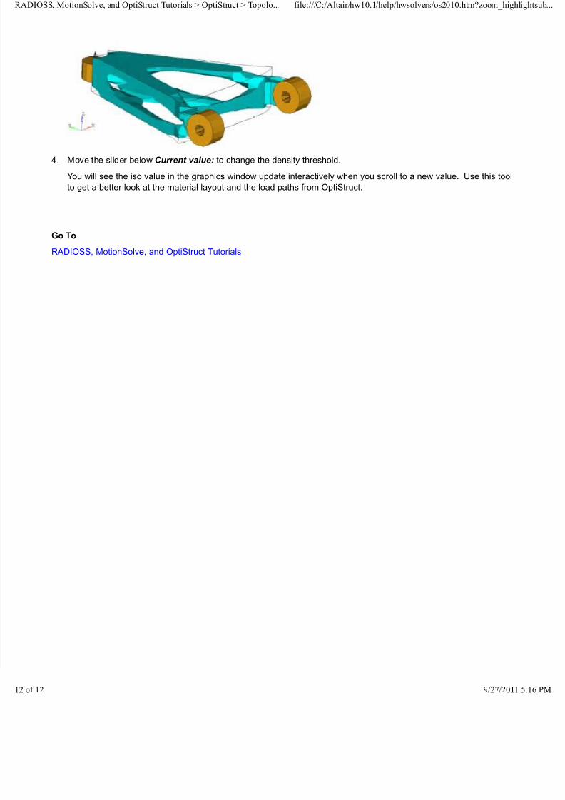
Step 15: View an Iso Value Plot on Top of the Element Densities Contour
This plot provides the information about the element density. Iso Value retains all of the elements at and above acertain density threshold. Pick the density threshold providing the structure that suits your needs.
1. From Graphics pull down menu, click on Iso Value, and choose Element Densities as the Result type.
2. Click Apply .
3. Set the Current Value: to 0.15.
IOSS, MotionSolve, and OptiStruct Tutorials > OptiStruct > Topolo... file:///C:/Altair/hw10.1/help/hwsolvers/os2010.htm?zoom_high
12 9/27/2011
7/29/2019 OS-2010 Design Concept for an Automotive Control Arm
http://slidepdf.com/reader/full/os-2010-design-concept-for-an-automotive-control-arm 12/12
4. Move the slider below Current value: to change the density threshold.
You will see the iso value in the graphics window update interactively when you scroll to a new value. Use this tool
to get a better look at the material layout and the load paths from OptiStruct.
Go To
RADIOSS, MotionSolve, and OptiStruct Tutorials
IOSS, MotionSolve, and OptiStruct Tutorials > OptiStruct > Topolo... file:///C:/Altair/hw10.1/help/hwsolvers/os2010.htm?zoom_high
Related Documents


![Antimicrobial Resistance Mitigation [ARM] Concept Paper · Antimicrobial Resistance Mitigation [ARM] Concept Paper Project Lead Vikesland (Civil and Environmental Engineering; COE).Development](https://static.cupdf.com/doc/110x72/5f5e3dce746e1c19960ec563/antimicrobial-resistance-mitigation-arm-concept-paper-antimicrobial-resistance.jpg)