Ordering Classifier Chains using filter model feature selection ...

Master of Science in Computer ScienceJune 2017

Ordering Classifier Chains using filtermodel feature selection techniques

Robin Gustafsson

Faculty of ComputingBlekinge Institute of TechnologySE–371 79 Karlskrona, Sweden

This thesis is submitted to the Faculty of Computing at Blekinge Institute of Technology inpartial fulfillment of the requirements for the degree of Master of Science in Computer Science.The thesis is equivalent to 20 weeks of full time studies.

Contact Information:Author(s):Robin GustafssonE-mail: [email protected]

University advisor:Dr. Hüseyin KusetoğullarıDepartment of Computer Science and Engineering

Faculty of Computing Internet : www.bth.seBlekinge Institute of Technology Phone : +46 455 38 50 00SE–371 79 Karlskrona, Sweden Fax : +46 455 38 50 57

Abstract

Context. Multi-label classification concerns classification with multi-dimensional output. The Classifier Chain breaks the multi-label probleminto multiple binary classification problems, chaining the classifiers to ex-ploit dependencies between labels. Consequently, its performance is influ-enced by the chain’s order. Approaches to finding advantageous chain ordershave been proposed, though they are typically costly.Objectives. This study explored the use of filter model feature selectiontechniques to order Classifier Chains. It examined how feature selectiontechniques can be adapted to evaluate label dependence, how such informa-tion can be used to select a chain order and how this affects the classifier’sperformance and execution time.Methods. An experiment was performed to evaluate the proposed ap-proach. The two proposed algorithms, Forward-Oriented Chain Selection(FOCS) and Backward-Oriented Chain Selection (BOCS), were tested withthree different feature evaluators. 10-fold cross-validation was performedon ten benchmark datasets. Performance was measured in accuracy, 0/1subset accuracy and Hamming loss. Execution time was measured duringchain selection, classifier training and testing.Results. Both proposed algorithms led to improved accuracy and 0/1subset accuracy (Friedman & Hochberg, p < 0.05). FOCS also improvedthe Hamming loss while BOCS did not. Measured effect sizes ranged from0.20 to 1.85 percentage points. Execution time was increased by less than3 % in most cases.Conclusions. The results showed that the proposed approach can im-prove the Classifier Chain’s performance at a low cost. The improvementsappear similar to comparable techniques in magnitude but at a lower cost.It shows that feature selection techniques can be applied to chain ordering,demonstrates the viability of the approach and establishes FOCS and BOCSas alternatives worthy of further consideration.

Keywords: multi-label classification, classifier chain, label dependence

i

Contents

Abstract i

1 Introduction 11.1 Aim and Objectives . . . . . . . . . . . . . . . . . . . . . . . . . . 21.2 Research Questions . . . . . . . . . . . . . . . . . . . . . . . . . . 2

2 Related Work 32.1 Fully Connected Chain Structures . . . . . . . . . . . . . . . . . . 42.2 Alternative Network Structures . . . . . . . . . . . . . . . . . . . 5

3 Preliminaries 83.1 Multi-label Classification . . . . . . . . . . . . . . . . . . . . . . . 8

3.1.1 Label Dependence . . . . . . . . . . . . . . . . . . . . . . 103.1.2 Performance Measures . . . . . . . . . . . . . . . . . . . . 10

3.2 Classifier Chain . . . . . . . . . . . . . . . . . . . . . . . . . . . . 123.2.1 Training and Prediction . . . . . . . . . . . . . . . . . . . 133.2.2 Chain Order . . . . . . . . . . . . . . . . . . . . . . . . . . 14

3.3 Feature Selection . . . . . . . . . . . . . . . . . . . . . . . . . . . 143.3.1 Feature Evaluation . . . . . . . . . . . . . . . . . . . . . . 15

4 Proposed Approach 174.1 Considerations . . . . . . . . . . . . . . . . . . . . . . . . . . . . 174.2 Proposed Algorithms . . . . . . . . . . . . . . . . . . . . . . . . . 18

4.2.1 Forward-Oriented Chain Selection . . . . . . . . . . . . . . 194.2.2 Backward-Oriented Chain Selection . . . . . . . . . . . . . 21

5 Method 235.1 Classifiers . . . . . . . . . . . . . . . . . . . . . . . . . . . . . . . 235.2 Datasets . . . . . . . . . . . . . . . . . . . . . . . . . . . . . . . . 245.3 Measurements . . . . . . . . . . . . . . . . . . . . . . . . . . . . . 26

6 Results 276.1 Classification Performance . . . . . . . . . . . . . . . . . . . . . . 276.2 Execution Time . . . . . . . . . . . . . . . . . . . . . . . . . . . . 30

ii

7 Analysis and Discussion 347.1 Classification Performance . . . . . . . . . . . . . . . . . . . . . . 347.2 Execution Time . . . . . . . . . . . . . . . . . . . . . . . . . . . . 367.3 Validity Threats and Limitations . . . . . . . . . . . . . . . . . . 38

8 Conclusions and Future Work 40

References 42

Appendix A Replication Data 50

iii

List of Figures

3.1 Examples of day-to-day multi-label situations . . . . . . . . . . . 93.2 A Classifier Chain with the default label order . . . . . . . . . . 12

6.1 Average effect sizes . . . . . . . . . . . . . . . . . . . . . . . . . . 30

7.1 Increases in execution time . . . . . . . . . . . . . . . . . . . . . 37

iv

List of Tables

5.1 Overview of the evaluated chain selectors . . . . . . . . . . . . . 245.2 Overview of the datasets . . . . . . . . . . . . . . . . . . . . . . . 255.3 Additional dataset metrics . . . . . . . . . . . . . . . . . . . . . . 25

6.1 FOCS classification performance, accuracy . . . . . . . . . . . . . 286.2 FOCS classification performance, 0/1 subset accuracy . . . . . . 286.3 FOCS classification performance, Hamming loss . . . . . . . . . . 286.4 BOCS classification performance, accuracy . . . . . . . . . . . . 296.5 BOCS classification performance, 0/1 subset accuracy . . . . . . 296.6 BOCS classification performance, Hamming loss . . . . . . . . . . 296.7 Label confusion (average) . . . . . . . . . . . . . . . . . . . . . . 306.8 FOCS execution time, chain order selection . . . . . . . . . . . . 316.9 FOCS execution time, training . . . . . . . . . . . . . . . . . . . 316.10 FOCS execution time, testing . . . . . . . . . . . . . . . . . . . . 316.11 BOCS execution time, chain order selection . . . . . . . . . . . . 326.12 BOCS execution time, training . . . . . . . . . . . . . . . . . . . 326.13 BOCS execution time, testing . . . . . . . . . . . . . . . . . . . . 32

v

List of Algorithms

1 The Classifier Chain training procedure . . . . . . . . . . . . . . 132 The Classifier Chain prediction procedure . . . . . . . . . . . . . 133 Forward-Oriented Chain Selection (FOCS) . . . . . . . . . . . . . 204 Backward-Oriented Chain Selection (BOCS) . . . . . . . . . . . . 21

vi

Chapter 1Introduction

In the field of machine learning, multi-label classification concerns the construc-tion of prediction models with multi-dimensional output. Each instance, consist-ing of a feature vector, is associated with a set of labels [49]. This contrasts withthe more common cases of binary and multi-class classification where the outputis a one-dimensional scalar.

Many different techniques exist for dealing with multi-label classification. Oneof them is the Classifier Chain. A Classifier Chain is constructed by dividing themulti-label classification task into multiple binary classification tasks, one foreach label. The feature space of each binary classifier is extended with the labelspredicted by the classifiers prior to itself in the chain. This lets the classifiersconsider previous labels as features, thus allowing label dependencies to influenceboth training and testing.

One aspect which influences the Classifier Chain’s classification performanceis the internal order of the chain’s nodes [33]. Some extensions to the ClassifierChain algorithm have considered chain ordering, e.g. [27, 38]. Other techniques forcalculating and exploiting label dependence have also been proposed for relatedalgorithms, e.g. [19, 56, 58].

These techniques have been criticized for being “over engineered” and theirviability has been questioned with regard to the offered performance increasein relation to the computational costs [42]. Meanwhile, computationally simplermethods based on probability and information metrics have shown positive resultsat a lower computational cost for related algorithms [42].

This study explores additional methods sharing some of the traits of the afore-mentioned, computationally cheaper methods. Specifically, the study focuses onadaptation of techniques used in filter model feature selection.

Drawing inspiration from feature selection is motivated by the typically goodscalability properties of such techniques, while the focus on filter model techniquesis chosen due to the similarity between them and the methods in [4, 28, 42].

1

Chapter 1. Introduction 2

1.1 Aim and ObjectivesThe aim of this study is to develop and evaluate extensions to the Classifier Chainalgorithm using concepts from filter model feature selection techniques. Morespecifically, the extensions consider the usage of such techniques to determine theorder of the chain’s nodes in an attempt to improve the chain’s predictive power.

To accomplish this aim, the following intermediate objectives are formulated:

• Examine existing methods for Classifier Chain ordering, identification oflabel dependencies and multi-label filter model feature selection techniques.

• Collect a set of benchmark datasets for multi-label classification.

• Select feature selection techniques suitable for adaption to the new task.

• Implement the adaptation technique.

• Run experiments to evaluate the performance of the ordered ClassifierChains across the set of benchmark datasets.

• Perform statistical analysis on the results.

1.2 Research QuestionsThe study answers the following research questions:

RQ1 How can filter model feature selection techniques be adapted to evaluatelabel dependence in multi-label data?

RQ2 How can label dependence evaluations be exploited when building a Clas-sifier Chain?

RQ3 How is the Classifier Chain’s classification performance affected?

RQ4 How is the Classifier Chain’s computational cost affected?

The first research question investigates if and how concepts used for featureselection can be used for evaluating label dependence in multi-label datasets. Thefocus lies on adapting concepts from filter model feature selection techniques tothe problem of evaluating label dependence.

The purpose of the second question is to explore the incorporation of labeldependence information in the construction process of a Classifier Chain. Itconsiders how the evaluations can be utilized to determine an order for the chain.

Finally, the third and fourth questions examine the effects of applying thesetechniques to Classifier Chains. The effects on both the predictive performanceand the computational cost is examined. These measurements will be used tocompare the chains built with prior knowledge of label dependencies to the orig-inal, implicitly ordered Classifier Chain.

Chapter 2Related Work

Since the introduction of the Classifier Chain algorithm, multiple extensions havebeen proposed to further improve the classification performance, e.g. [6, 27, 38,55]. The extensions primarily focus on two separate aspects of the ClassifierChain: the induction procedure and the issue of label ordering. Of the two, onlythe latter is of real interest to this study. A few related algorithms have alsobeen proposed based on the Classifier Chain’s base concept of connecting binaryclassifier, albeit with different network structures, e.g. [21, 28, 42, 56].

One extension which has gotten attention in recent literature is the Proba-bilistic Classifier Chain (PCC) [6] and its variations, such as the Beam SearchPCC [27] and the ε-approximation PCC [7]. These extensions focus on the induc-tion procedure, replacing the greedy approach in the original algorithm to reducethe chain order’s significance. As they do not pay particular attention to labelordering, most of them will not be examined further in this study. Only the BeamSearch variant [27] will be included, as it simultaneously addresses label orderingthrough additional changes.

Another common approach to counteract the label order issue is the use ofensemble methods. The Ensemble of Classifier Chains [40, 41] was proposed toavoid the issue by using multiple randomized Classifier Chains. This approach haslater been extended in various ways [29, 38]. Some ensemble methods have alsobeen proposed where different Classifier Chains are used for different instances [4,46]. The ensembles are generally oriented towards reducing the impact of the labelorder by using multiple chains. As such, they are not directly applicable to thisstudy and will not be further examined, either.

Of particular interest to this study are existing approaches to label ordering.This includes some of the extensions to the Classifier Chain algorithm and itsrelatives. For further discussion, we differentiate between those that retain thefully connected chain structure and those that connect the labels using differentnetwork structures.

3

Chapter 2. Related Work 4

2.1 Fully Connected Chain StructuresThe methods proposed in this study focus on ordering fully connected ClassifierChains. As such, methods retaining the fully connected Classifier Chain structureare of primary interest.

One such method is the aforementioned Beam Search PCC [26, 27]. Whileprimarily oriented towards the induction procedure (building on PCC), the pro-posed method also tackles the chain ordering problem through the use of BeamSearch. The space of possible chains is modeled as a tree and a scoring functionsis used to evaluate the quality of various chain configurations. Scoring functionsusing both kernel target alignment and the validation error of a trained PCCare tried, with the former showing better results both in terms of classificationperformance and computational cost [26].

In [38], the chain order is instead determined using a Monte Carlo searchtechnique. A random initial chain is chosen, which is then mutated for a pre-determined number of iterations. In each iteration, two nodes are swapped, thechain’s quality is determined and the new chain is kept if its score exceeds thepreviously best one. Each chain order’s score is determined by training and eval-uating a new Classifier Chain model.

A somewhat similar approach is the use of a genetic algorithm in [20]. Aninitial population of randomly ordered Classifier Chains is created. Afterwards,a random selection is made and the selected chains are evaluated. The best arechosen to produce the next generation through cross-over and random mutations.After a pre-determined number of generations, the single best chain is chosen.

Finally, a completely different approach is presented in [54, 55]. There, k-means clustering is employed to divide the data into two groups. Each label isgiven a score based on how well the clusters represent the existence/absence ofthe label. A Classifier Chain is then built with the labels ordered by their scores,in descending order.

A need for a larger number of iterations is noted for the Monte Carlo approachto be effective on data sets with many labels [38]. The increased number of itera-tions is computationally problematic as each iteration also increases in complexitywith the number of labels. This is a side-effect of training and evaluating a Clas-sifier Chain in each iteration, as the cost of both training and prediction increaseswith the number of labels (as evident from algorithms 1 and 2). While not explic-itly discussed in [20], the same problem possibly affects the evolutionary approach.The evolution process entails training and evaluation of a large number of can-didate chains (the number of generations times the population size) [20]. Thisappears to have limited the values of both factors for evaluations on mediumand large datasets in the study. A similar drawback regarding computationalcost is also noted for Beam Search PCC when involving classifiers in the scoringfunction [26, 27].

The obvious difference between the k-means approach and the others is the


use of clustering rather than search techniques. Another notable aspect is that itorders the labels with a different objective in mind. Rather than considering theactual/estimated effects of various orders, it attempts to gauge the predictabilityof labels prior to chaining. The chain is then constructed such that the most pre-dictable labels (according to the estimations) are predicted first. The underlyingassumption is that those labels are more likely to be correctly predicted, thuslowering the risk of errors cascading along the chain [55].

Positive influence on classification performance is reported for all of the meth-ods [20, 26, 27, 38, 54, 55]. In most cases, the same is concluded about the labelordering aspect in isolation. The notable exception is the clustering approach [54,55]. There, other changes are introduced simultaneously without any attempts toisolate their respective effects. As such, the label ordering approach’s success can-not be reliably determined as the positive results may stem from other aspectsof the method. This is especially unfortunate as it takes a radically differentapproach to the problem than the other methods.

None of the discussed methods use measures akin to those developed in thisstudy to order the chains. The most similar ones are the kernel target alignmentand the k-means clustering, as those do not directly involve classification modelsin their evaluations. Other than that, they have little in common.

In summary, the discussed methods for ordering fully connected chains un-derline the value of explicit label ordering. At the same time, they also indicatethat scalability may be problematic if the order is determined by evaluating themany candidate chains. Doing so may also not guarantee the best results, thougha comparison has only been presented for one of the algorithms [26, 27].

2.2 Alternative Network StructuresIn addition to the Classifier Chain extensions, previous literature has also pro-posed related algorithms with modified network structures. The chain structureis then replaced by a directed acyclic graph or tree structure. While this studyfocuses on the Classifier Chain, the approaches used to model label dependencein the related algorithms are still interesting.

One of the related algorithms is the Bayesian Classifier Chain [56]. It exploresa different way to model label dependence, revolving around Bayesian Networks.A Bayesian Network is created to model the labels’ dependencies based on condi-tional probabilities. A tree-like structure of binary classifiers is then constructedbased on the network. A few other approaches for modeling label dependence asBayesian networks [19, 58] have in turn been used to create alternative versionsof the Bayesian Classifier Chain [42].

Bayesian networks are also utilized in [35] and [28]. In [35], the network iscreated in a simpler way using only fully deterministic relationships, i.e. caseswhere some labels either always or never co-exist. In [28], a Bayesian network


inference algorithm is adapted to maximize the conditional entropy metric insteadof the conditional probability.

Previous work also propose some alternative structures without using Bayesiannetworks. In [21], the genetic algorithm approach from [20] is extended to alsoconsider partially connected chains. In such partial chains, some labels are dis-connected from each other or from the network as a whole. In [4], a graph isconstructed based on the mutual information metric and a maximum spanningtree is constructed from the graph. The network is constructed based on the tree,where each classifier’s feature space is augmented with the labels predicted by allof its ancestors in the tree.

Finally, there is the Classifier Trellis algorithm [42]. The Classifier Trellisdiffers from all previously mentioned algorithms in this section as it does notattempt to find a structure. Rather, it uses a fixed structure and attempts toplace the labels optimally within this structure. It evaluates a label’s suitabilityfor a particular position using the mutual information metric between it and thepotential parents.

Overall, a preference for Bayesian networks as a way of modeling label depen-dence is seen in the related literature, with most of the aforementioned studiestaking this approach [19, 35, 56, 58]. The Bayesian network is a well-known wayto model dependencies in Bayesian statistics, making this focus understandable.However, finding the graph structures can be expensive, especially for a highnumber of variables (such as for datasets with a large numbers of labels) [42].In fact, when some of these methods were compared to other alternatives, it wasconcluded that the offered performance did not necessarily warrant the high com-putational complexity [42]. The more complex methods did not guarantee betterclassification performance than some computationally simpler methods [42].

Of great importance to this study is also the fact that such network struc-tures are not applicable to the original Classifier Chain algorithm – hence whythey have been evaluated only on the related Bayesian Classifier Chain. Theoriginal Classifier Chain algorithm imposes a fixed network structure and so thestructure does not need to be found. Replacing the Classifier Chain algorithm’snetwork structure with that found through the construction of a Bayesian net-work essentially turns it into the Bayesian Classifier Chain algorithm. The factthat the network structure is fixed by the Classifier Chain algorithm reduces theproblem to that of finding the most suitable fit (i.e. the best chain order). Thisis equally true for the Classifier Trellis algorithm, where a similar insight playedan integral part in the algorithm’s design [42].

In relation to the Classifier Chain algorithm, the Classifier Trellis is the mostsimilar as both use fixed structures. The Classifier Trellis successfully applied thepairwise mutual information metric to order its labels [42], suggesting that thesame could possibly work well for label ordering in the Classifier Chain.

Despite the differences in network structure, some similarities exist betweenthe reviewed methods and those proposed in this study. Generally, the reviewed


algorithms make use of various metrics to find the optimal network structure orlabel ordering. This is similar to the metrics-based approach taken in this study.It contrasts with the methods presented in section 2.1, where the most commonapproach was to evaluate a multitude of candidate classifiers. Specifically, some ofthe methods make use of conditional entropy [28] and mutual information [4, 42].Both metrics are commonly applied in filter model feature selection techniques.Furthermore, the Bayesian networks are based on conditional probability, whichis also at the foundation of many filter model feature selection techniques.

Chapter 3Preliminaries

This study is performed within the area of multi-label classification. Primarily,it revolves around the concept of label dependence and the Classifier Chain algo-rithm. Additionally, it involves methods for filter model feature selection. Theseareas are described and defined in the following sections.

3.1 Multi-label ClassificationMulti-label classification is a type of classification where the output is a set oflabels [49]. This contrasts with the more common cases of binary or multi-classclassification, where the output is either a single binary or nominal value.

This type of learning task was originally popularized for text categorization,but has since been utilized in many other fields for things such as medical di-agnosis, protein function classification, music categorization and image recogni-tion [49]. It is applicable whenever an instance can belong to more than onecategory or be assigned multiple characteristics. A few examples of such situa-tions are shown in fig. 3.1.

In multi-label classification, as in binary and multi-class classification, eachinstance is associated with a feature vector. The feature vector contains all the in-put values representing that instance. Based on the feature vector, a constructedmodel is tasked with determining the classification of the instance. Contrary tobinary and multi-class classification, the instances in multi-label classification areto be associated with a set of labels.

The formal definition and the used notation varies throughout the multi-labelliterature [41, 42, 49]. The following definition and notation will be used through-out this report: A multi-label classification task consists of a feature space X anda set of L possible labels L = {y1, y2, ..., yL}. Each label y is a binary variablesuch that y ∈ {0, 1}. Each instance consists of a feature vector x ∈ X and isassociated with a set of labels y ⊆ L. A classifier H : X → L is learned fromthe set of D training instances D = {(x1,y1), (x2,y2), ..., (xD,yD)}. The trainedclassifier can then induce a predicted label set y from the feature vector x of apreviously unseen instance; y = H(x).

8

Chapter 3. Preliminaries 9

Figure 3.1: Examples of day-to-day multi-label situations: a programming ques-tion involving multiple topics (top), music spanning multiple genres (bottom) anda video game possessing multiple characteristics (right).


Many different techniques exist for dealing with multi-label classification.In addition to algorithms created specifically for multi-label classification (e.g.AdaBoost.MH [43] and LIFT [57]), problem transformation methods (e.g. Bi-nary Relevance [3] and Label Powerset [51]) exist to transform the problem intobinary or multi-class classification tasks.

The most commonly used problem transformation method is Binary Rele-vance [51]. In Binary Relevance, the multi-label task is divided into one binaryclassification task for each label. Each binary classifier predicts the existence ofa single label. These individual predictions are then combined to form the setof predicted labels. This technique has been widely applied but has often beencriticized for its inability to consider label dependence [32, 41], giving rise to othermethods such as Classifier Chains.

3.1.1 Label Dependence

Label dependence (sometimes called label correlation) is a natural part of manymulti-label classification tasks. For example, in a text categorization task, itis plausible that the label Religion would perhaps often co-exist with the labelHistory, while also implying the absence of the Engineering label. Consequen-tially, the consideration of such dependencies is generally seen as important forachieving good classification performance [8, 34, 40].

Label dependence can be divided into two categories; marginal label depen-dence and conditional label dependence [8]. Marginal label dependence modelsthe label dependence with regards to the specific instances [8]. It can be measuredas the labels’ co-occurrence frequency [42]. Conditional label dependence, on theother hand, models the global dependence between labels and is independent ofany particular instance [8]. It is more complex to measure, as the entire featurespace must be taken into account [42].

3.1.2 Performance Measures

A multitude of classification performance measures have been proposed in multi-label literature. Some of the commonly used ones are accuracy, 0/1 subset accu-racy and Hamming loss.

Accuracy

Accuracy measures the average ratio of correctly classified labels to the totalnumber of labels in the predicted and the true label sets [18]. The accuracy scoreis the averaged score across all test instances. It takes a value in the range of zeroto one (inclusive), with an optimal value of one.


The accuracy is defined as

1

N

N∑i=1

|yi ∩ yi||yi ∪ yi|

,

where N is the number of instances in the test set, yi is the true label set and yiis the predicted label set for the ith instance.

The multi-label accuracy measure is not to be confused with accuracy as usedin the context of binary or multi-class classification.

0/1 Subset Accuracy

0/1 subset accuracy measures the fraction of instances whose labels are perfectlypredicted [17, 60]. It takes a value in the range of zero to one (inclusive), withan optimal value of one.

The measure is very strict as it does not distinguish between partially correctand completely incorrect predictions [17]. An instance is given a score of one ifall labels are correctly predicted, or zero otherwise. The final score is the averageacross all instances.

0/1 subset accuracy is defined as

1

N

N∑i=1

Jyi = yiK,

where N is the number of instances in the test set and Jyi = yiK evaluates to oneif the two sets are equal, or to zero if they are not.

0/1 subset accuracy is sometimes referred to as classification accuracy or exactmatch ratio [17, 60]. It is also the complement of the 0/1 loss measure, whichmeasures the fraction of instances whose labels are not perfectly predicted.

Hamming Loss

Hamming loss measures the average fraction of misclassified labels across all testinstances [17, 44]. It takes a value in the range of zero to one (inclusive), with anoptimal value of zero.

A partially correct labeling of an instance is awarded with a score proportionalto the ratio of correctly classified labels. It can be interpreted as the average errorrate on L separate binary classification tasks, one for each label [44].

Hamming loss is calculated as

1

N

N∑i=1

|yi4yi|L

,

where N is the number of instances in the test set, L is the number of labels, andy4y represents the disjunctive union of the two label sets, i.e. the labels foundin one of the sets but not in both.


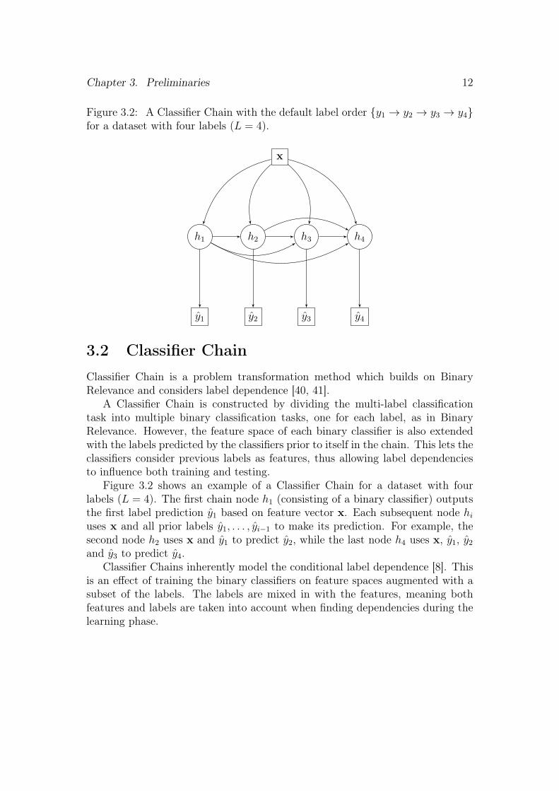
Figure 3.2: A Classifier Chain with the default label order {y1 → y2 → y3 → y4}for a dataset with four labels (L = 4).

x

h1 h2 h3 h4

y1 y2 y3 y4

3.2 Classifier ChainClassifier Chain is a problem transformation method which builds on BinaryRelevance and considers label dependence [40, 41].

A Classifier Chain is constructed by dividing the multi-label classificationtask into multiple binary classification tasks, one for each label, as in BinaryRelevance. However, the feature space of each binary classifier is also extendedwith the labels predicted by the classifiers prior to itself in the chain. This lets theclassifiers consider previous labels as features, thus allowing label dependenciesto influence both training and testing.

Figure 3.2 shows an example of a Classifier Chain for a dataset with fourlabels (L = 4). The first chain node h1 (consisting of a binary classifier) outputsthe first label prediction y1 based on feature vector x. Each subsequent node hiuses x and all prior labels y1, . . . , yi−1 to make its prediction. For example, thesecond node h2 uses x and y1 to predict y2, while the last node h4 uses x, y1, y2and y3 to predict y4.

Classifier Chains inherently model the conditional label dependence [8]. Thisis an effect of training the binary classifiers on feature spaces augmented with asubset of the labels. The labels are mixed in with the features, meaning bothfeatures and labels are taken into account when finding dependencies during thelearning phase.


3.2.1 Training and Prediction

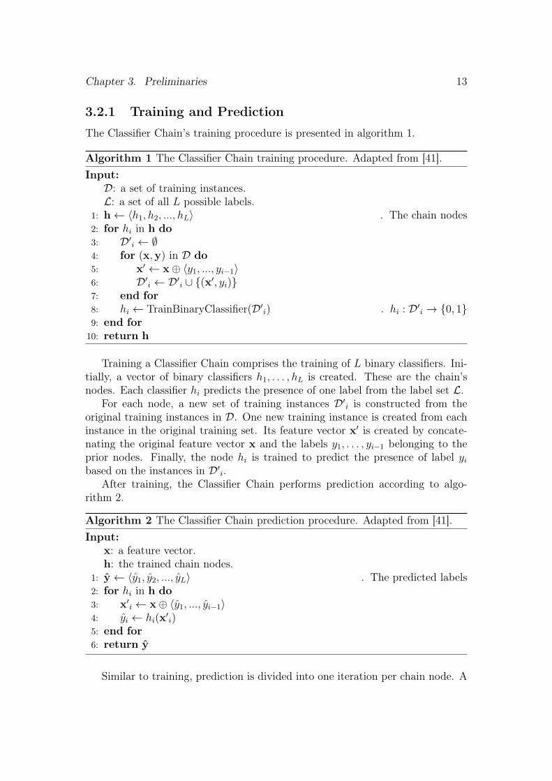
The Classifier Chain’s training procedure is presented in algorithm 1.

Algorithm 1 The Classifier Chain training procedure. Adapted from [41].Input:D: a set of training instances.L: a set of all L possible labels.

1: h← 〈h1, h2, ..., hL〉 . The chain nodes2: for hi in h do3: D′i ← ∅4: for (x,y) in D do5: x′ ← x⊕ 〈y1, ..., yi−1〉6: D′i ← D′i ∪ {(x′, yi)}7: end for8: hi ← TrainBinaryClassifier(D′i) . hi : D′i → {0, 1}9: end for

10: return h

Training a Classifier Chain comprises the training of L binary classifiers. Ini-tially, a vector of binary classifiers h1, . . . , hL is created. These are the chain’snodes. Each classifier hi predicts the presence of one label from the label set L.

For each node, a new set of training instances D′i is constructed from theoriginal training instances in D. One new training instance is created from eachinstance in the original training set. Its feature vector x′ is created by concate-nating the original feature vector x and the labels y1, . . . , yi−1 belonging to theprior nodes. Finally, the node hi is trained to predict the presence of label yibased on the instances in D′i.

After training, the Classifier Chain performs prediction according to algo-rithm 2.

Algorithm 2 The Classifier Chain prediction procedure. Adapted from [41].Input:

x: a feature vector.h: the trained chain nodes.

1: y← 〈y1, y2, ..., yL〉 . The predicted labels2: for hi in h do3: x′i ← x⊕ 〈y1, ..., yi−1〉4: yi ← hi(x

′i)

5: end for6: return y

Similar to training, prediction is divided into one iteration per chain node. A


new feature vector is constructed in a similar manner as during training. How-ever, the true labels y are unknown at prediction time. Instead, the predictionsy1, . . . , yi−1 made by the prior nodes are used when extending the feature vector.The new feature vector x′i is then used by hi to make its prediction yi.

3.2.2 Chain Order

One factor influencing the performance of the Classifier Chain is the chain or-der [40, 41]. The chain order concerns the order in which the various labels arepredicted. It thus also determines which labels are available as features whenpredicting a subsequent label. The order must be established at training time.

The underlying theoretical concept, the product rule of probability, impliesthat the order does not matter [33]. However, as the actual classifiers are butapproximations of the true probabilities, the order does in fact matter in prac-tice [33, 46]. This follows from the fact that classifiers in different parts of thechain operate on different feature spaces [8].

The original Classifier Chain algorithm does not attempt to optimize thechain’s order. Typically, the label order in the dataset is kept unchanged. Alter-natively, the labels may be (randomly) reorganized prior to training.

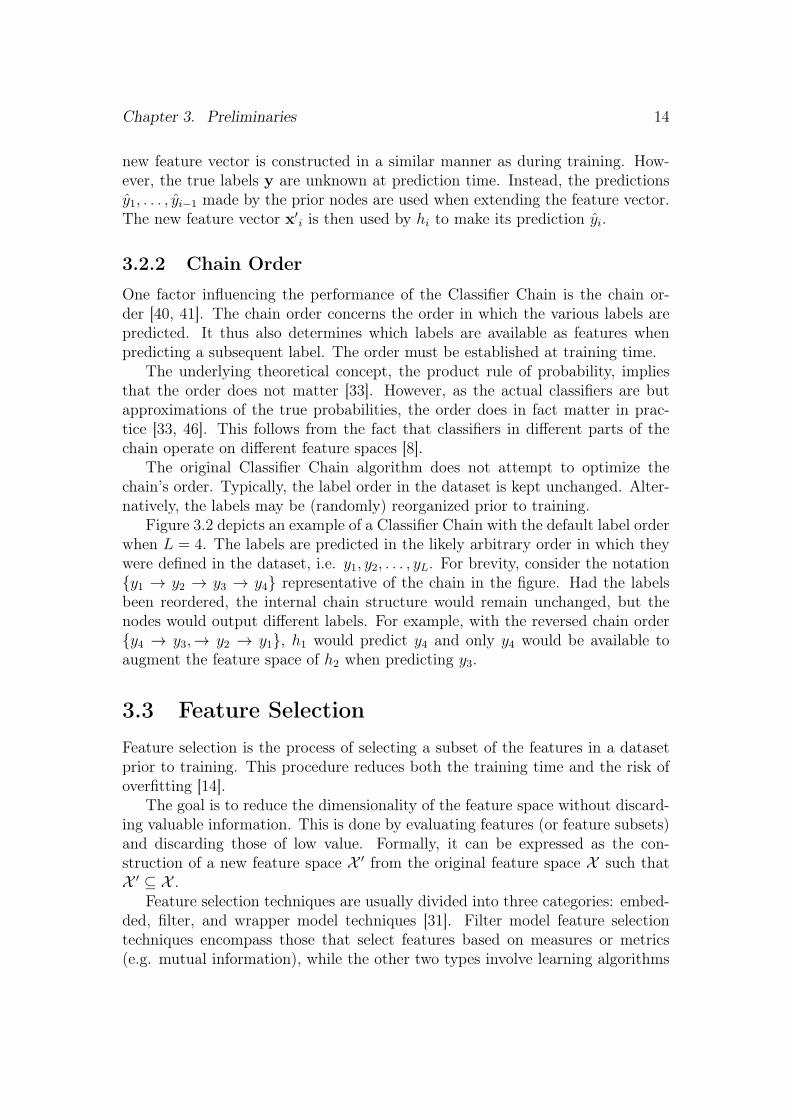
Figure 3.2 depicts an example of a Classifier Chain with the default label orderwhen L = 4. The labels are predicted in the likely arbitrary order in which theywere defined in the dataset, i.e. y1, y2, . . . , yL. For brevity, consider the notation{y1 → y2 → y3 → y4} representative of the chain in the figure. Had the labelsbeen reordered, the internal chain structure would remain unchanged, but thenodes would output different labels. For example, with the reversed chain order{y4 → y3,→ y2 → y1}, h1 would predict y4 and only y4 would be available toaugment the feature space of h2 when predicting y3.

3.3 Feature SelectionFeature selection is the process of selecting a subset of the features in a datasetprior to training. This procedure reduces both the training time and the risk ofoverfitting [14].

The goal is to reduce the dimensionality of the feature space without discard-ing valuable information. This is done by evaluating features (or feature subsets)and discarding those of low value. Formally, it can be expressed as the con-struction of a new feature space X ′ from the original feature space X such thatX ′ ⊆ X .

Feature selection techniques are usually divided into three categories: embed-ded, filter, and wrapper model techniques [31]. Filter model feature selectiontechniques encompass those that select features based on measures or metrics(e.g. mutual information), while the other two types involve learning algorithms


directly [31]. The filter model category is the most popular one in multi-labelliterature [36, 47].

In the multi-label classification context, a different categorization is also usedto distinguish direct feature selection techniques from transformation-based tech-niques [36]. This division mirrors that of the classifiers themselves; while sometechniques apply directly to the multi-label case, others are applied by trans-forming the multi-label classification dataset to binary or multi-class classificationdatasets.

One particularly popular transformation-based approach is that based on thebinary relevance transform [36]. The multi-label problem is divided into multiplebinary classification problems. A feature selection measure for binary classifica-tion is then applied separately to each sub-problem. The results for each sub-problem are then aggregated to create the final result, typically by averaging ormaximization [36].

3.3.1 Feature Evaluation

To select a good set of features, the features must be evaluated in some way. Theway in which features are evaluated is typically the defining aspect of a featureselection technique. Examples of commonly employed measures and methods aremutual information, the χ2 statistic and ReliefF [36, 48].

Mutual Information

Mutual information measures the amount of information shared by two vari-ables [11]. The mutual information I(X;Y ) of the two variables X and Y isdefined as

I(X;Y ) =∑x∈X

∑y∈Y

p(x, y) log2

p(x, y)

p(x)p(y)

where p(x) and p(y) are the marginal probabilities and p(x, y) is the joint prob-ability of X and Y taking the values x and y, respectively [5].

The measure stems from information theory and is derived from the widespreadentropy measure [5]. Entropy measures a variable’s level of uncertainty [45]. Interms of entropy, mutual information can be expressed as

I(X;Y ) = H(X)−H(X|Y )

where H(X) is the entropy of X and H(X|Y ) is the entropy of X given the valueof Y [5]. It can thus also be interpreted as measuring the decrease in a variable’suncertainty given the value of another [5].

Mutual information is also known as information gain within the context ofmachine learning [59].


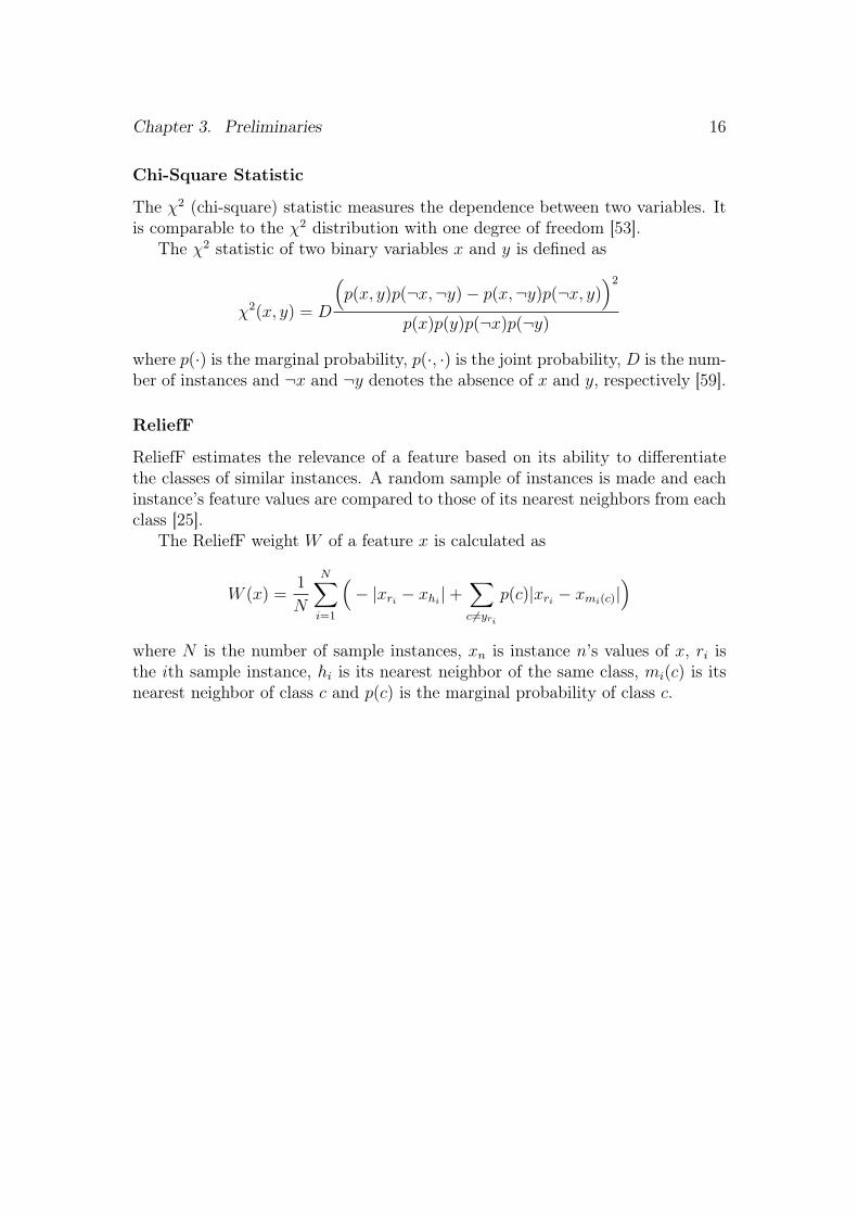
Chi-Square Statistic

The χ2 (chi-square) statistic measures the dependence between two variables. Itis comparable to the χ2 distribution with one degree of freedom [53].

The χ2 statistic of two binary variables x and y is defined as

χ2(x, y) = D

(p(x, y)p(¬x,¬y)− p(x,¬y)p(¬x, y)

)2p(x)p(y)p(¬x)p(¬y)

where p(·) is the marginal probability, p(·, ·) is the joint probability, D is the num-ber of instances and ¬x and ¬y denotes the absence of x and y, respectively [59].

ReliefF

ReliefF estimates the relevance of a feature based on its ability to differentiatethe classes of similar instances. A random sample of instances is made and eachinstance’s feature values are compared to those of its nearest neighbors from eachclass [25].

The ReliefF weight W of a feature x is calculated as

W (x) =1

N

N∑i=1

(− |xri − xhi|+

∑c6=yri

p(c)|xri − xmi(c)|)

where N is the number of sample instances, xn is instance n’s values of x, ri isthe ith sample instance, hi is its nearest neighbor of the same class, mi(c) is itsnearest neighbor of class c and p(c) is the marginal probability of class c.

Chapter 4Proposed Approach

The proposed approach revolves around the use of various dependency measuresto determine the Classifier Chain’s internal order. The measures are adapted fromfilter model feature selection techniques to instead evaluate label dependence.

The motivation behind focusing on adapting feature selection techniques is,firstly, the likeness to the approach used in [42] and the metrics used in [4, 28].Secondly, it is motivated by the belief that such techniques would offer advanta-geous scalability and computational complexity. Scalability to high-dimensionaldata is a highly desired property of feature selection techniques, as the need forfeature selection is often greater in such cases. Meanwhile, the number of labelsis typically lower than the number of features in a multi-label dataset. Thus, theassumption is that concepts from feature selection has the potential to also beapplied to labels at a relatively low computational cost.

4.1 ConsiderationsAdaptation of feature selection techniques to chain ordering requires the gapbetween the two problems to be bridged. The fundamental difference is thechange in evaluation subject. In feature selection, features are evaluated basedon their influence on labels. In the chain ordering case, we instead evaluate labelsbased on their influence on other labels.

To avoid terminological confusion, let inputs denote the evaluation subjects,e.g. the features in feature selection. Similarly, let outputs denote the values tobe predicted, e.g. the labels in feature selection.

The change in subject leads to two main aspects to address: Firstly, in featureselection, a subset of the feature space is selected. Doing so entails a discardingof inputs. In chain ordering, we cannot discard inputs as they are labels, all ofwhich shall be included in the chain. Secondly, during feature selection, the inputset changes in each step while the output set remains constant. The input setand the output set are also fundamentally distinct, belonging to the feature spaceand the label space, respectively. In chain ordering, the input set and output setconstitute a partition of the label set. Each step moves one label from the outputset to the input set. Both sets are thus variable.

17

Chapter 4. Proposed Approach 18

The first of these aspects means that we are no longer interested in finding asubset. Rather, we are focused only on the order in which the inputs are selected.This limits us to feature selection techniques capable of ranking inputs individ-ually rather than in groups or entire subsets. This is of little concern as featureselection algorithms commonly operate on individual features. The second aspectmeans we cannot rank all inputs at once. Instead, the process can be thought ofas iteratively selecting the single best input from several different datasets. Thisreformulation imposes no further limitations on the feature selection algorithmsconsidered for adaptation. However, it may be a detriment to the scalabilityunless changes to the dataset are handled efficiently.

Finally, there is the separate issue of the direction in which labels are evalu-ated. On the one hand, a candidate label could be selected based on how well itpredicts subsequent labels. On the other hand, it could instead be selected basedon how well it can be predicted by the previous labels. This dualism has beenbriefly mentioned, but not directly addressed, in previous literature [26, 27].

4.2 Proposed AlgorithmsTwo separate, albeit similar, algorithms are proposed. Both algorithms share thesame general outline but evaluate labels in opposite directions.

A transformation is applied to the dataset to turn the label dependence eval-uation problem into a collection of feature evaluation problems. The transformeddatasets can be used in conjunction with regular feature selection techniques forbinary classification to evaluate label dependencies. A chain order is then selectedbased on the evaluation results, by iteratively choosing the label which is deemedbest with regards to the results. The selected chain order is then passed as aparameter to the Classifier Chain prior to training. Consequently, the classifieris constructed in an order believed to better exploit the dependencies betweenlabels.

The proposed algorithms can be outlined in the following steps:

1. A label evaluation dataset is created from the regular multi-label dataset.The feature vector of every instance is discarded and replaced by a copy ofthe label vector. That is, the dataset D = {(x,y)}D is transformed into anew dataset D′ = {(y,y)}D.

2. A binary relevance transform is applied to the label evaluation dataset. Lbinary classification datasets are created, each with a single binary output.

3. Every feature in every binary classification dataset is evaluated, except forthe combinations where both the feature and the class refer to the samelabel. Evaluation is performed using a regular feature evaluation function,as normally used for feature selection. The evaluation function maps a


feature to a real number expressing its level of influence over the class,based on the information contained in the dataset.

4. The labels are iteratively chosen. At each step, the candidate label withthe best score is selected. This repeats until all labels have been chosen.The score is an aggregate of the scores received during the evaluation. Theway in which the scores are aggregated differs between the two proposedalgorithms.

The binary transform allows every label-label pair to be evaluated separately.This alleviates the complications of having a variable label set. Changes to thelabel set can instead be accounted for by altering which values are included inthe aggregated score.

The feature evaluation function can be any function capable of evaluating asingle feature’s influence over a single label in a given dataset. However, theprime examples of such functions are those used for filter model feature selectionin binary classification, e.g. those described in section 3.3.1.

This approach’s primary strength is that the feature evaluation algorithms re-main unchanged. No specialized adaptation of individual measures or algorithmsis required. It is also highly practical as existing implementations of featureevaluators can be used without modification.

The transformation technique estimates the marginal label dependence as itdoes not consider the features’ impact on the labels.

4.2.1 Forward-Oriented Chain Selection

The first algorithm selects labels based on how well they predict subsequent labels.Based on this property of looking forward at the remaining labels, it will bereferred to as Forward-Oriented Chain Selection, or FOCS for short. It is definedin algorithm 3.

FOCS evaluates a label (an input) based on its ability to predict future labels(outputs). It does so while ignoring the influence of previously selected labels(other inputs). This is akin to how most multi-label filter model feature selectionalgorithms work [30]. A candidate label’s value is the sum of its influence overall other remaining labels.

In comparison to techniques from related work, FOCS has most in commonwith the techniques employed in the Beam Search PCC [26, 27] and the Classi-fier Trellis [42]. FOCS can be framed as performing a greedy search across thesame search tree as the Beam Search PCC, albeit with a different type of evalua-tion function. The Classifier Trellis uses a more similar evaluation function, butit constructs a different network structure and operates in a backward-orientedmanner. That is, it evaluates the previous labels’ influence on the candidate labelinstead.


Algorithm 3 Forward-Oriented Chain Selection (FOCS)Input:D: a dataset of training instances.M : a feature evaluation function.

1: D′ ← CreateLabelEvaluationDataset(D) . Replace features with labels2: for all y ∈ L do3: D′y ← BinaryRelevanceTransform(D′, y) . Make y the only output4: for all c ∈ L do5: if c 6= y then6: Vc,y ←M(D′y, c) . Evaluate c’s ability to predict y7: end if8: end for9: end for

10: f ← 〈〉 . The vector of ordered labels11: S ← L . The set of remaining labels12: while S 6= ∅ do13: for all c ∈ S do14: S ′ ← S \ {c}15: Vc ←

∑y∈S′ Vc,y . c’s current total value

16: end for17: cmax ← argmaxc∈S Vc . Select the best candidate18: f ← f ⊕ 〈cmax〉19: S ← S \ {cmax}20: end while21: return f


4.2.2 Backward-Oriented Chain Selection

The second algorithm selects labels based on how well they are predicted byprevious labels. As this can be likened to looking backwards in the chain, it willbe referred to as Backward-Oriented Chain Selection, or BOCS. It is defined inalgorithm 4.

Algorithm 4 Backward-Oriented Chain Selection (BOCS)Input:D: a dataset of training instances.M : a feature evaluation function.

1: D′ ← CreateLabelEvaluationDataset(D) . Replace features with labels2: for all y ∈ L do3: D′y ← BinaryRelevanceTransform(D′, y) . Make y the only output4: for all c ∈ L do5: if c 6= y then6: Vc,y ←M(D′y, c) . Evaluate c’s ability to predict y7: end if8: end for9: end for

10: cfirst ← SelectRandom(L) . Randomly select the first label11: f ← 〈cfirst〉 . The vector of ordered labels12: S ← L \ {cfirst} . The set of remaining labels13: while S 6= ∅ do14: for all c ∈ S do15: Vc ←

∑y∈f Vy,c . c’s current total value

16: end for17: cmax ← argmaxc∈S Vc . Select the best candidate18: f ← f ⊕ 〈cmax〉19: S ← S \ {cmax}20: end while21: return f

BOCS selects a label based on its predictability (i.e. as an output) given thepreviously selected labels (inputs). A candidate label’s value is the sum of allpreviously selected labels’ influence over it.

Taking this perspective causes uncertainty as to how the first label should bechosen. Due to the absence of previously selected labels, all candidates appearto be equally valid choices. In BOCS, this is solved by selecting the first labelat random. This solution is both intuitive and simple, and has previously beensuccessfully used for ordering Classifier Trellises [42].

In relation to previous work, BOCS more closely resembles the Classifier Trel-lis’ ordering procedure [42] than a feature selection procedure. BOCS differs from


the Classifier Trellis’ approach as it considers a fully connected chain structureand is flexible with regards to the used evaluation measure.

Chapter 5Method

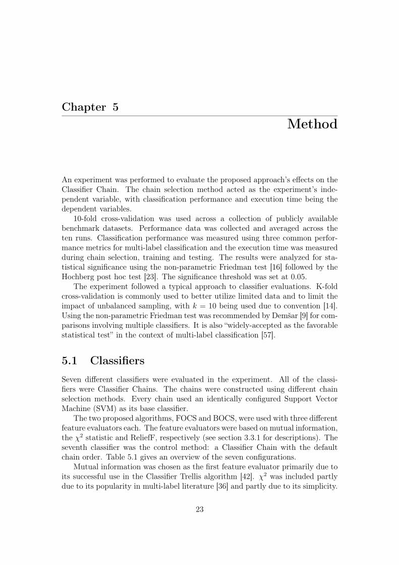
An experiment was performed to evaluate the proposed approach’s effects on theClassifier Chain. The chain selection method acted as the experiment’s inde-pendent variable, with classification performance and execution time being thedependent variables.

10-fold cross-validation was used across a collection of publicly availablebenchmark datasets. Performance data was collected and averaged across theten runs. Classification performance was measured using three common perfor-mance metrics for multi-label classification and the execution time was measuredduring chain selection, training and testing. The results were analyzed for sta-tistical significance using the non-parametric Friedman test [16] followed by theHochberg post hoc test [23]. The significance threshold was set at 0.05.

The experiment followed a typical approach to classifier evaluations. K-foldcross-validation is commonly used to better utilize limited data and to limit theimpact of unbalanced sampling, with k = 10 being used due to convention [14].Using the non-parametric Friedman test was recommended by Demšar [9] for com-parisons involving multiple classifiers. It is also “widely-accepted as the favorablestatistical test” in the context of multi-label classification [57].

5.1 ClassifiersSeven different classifiers were evaluated in the experiment. All of the classi-fiers were Classifier Chains. The chains were constructed using different chainselection methods. Every chain used an identically configured Support VectorMachine (SVM) as its base classifier.

The two proposed algorithms, FOCS and BOCS, were used with three differentfeature evaluators each. The feature evaluators were based on mutual information,the χ2 statistic and ReliefF, respectively (see section 3.3.1 for descriptions). Theseventh classifier was the control method: a Classifier Chain with the defaultchain order. Table 5.1 gives an overview of the seven configurations.

Mutual information was chosen as the first feature evaluator primarily due toits successful use in the Classifier Trellis algorithm [42]. χ2 was included partlydue to its popularity in multi-label literature [36] and partly due to its simplicity.

23

Chapter 5. Method 24

Table 5.1: Overview of the evaluated chain selectors

Chain selector Feature evaluator

Control None None

FOCSMI FOCS Mutual informationFOCSχ2 FOCS χ2 statisticFOCSRF FOCS ReliefF

BOCSMI BOCS Mutual informationBOCSχ2 BOCS χ2 statisticBOCSRF BOCS ReliefF

Finally, ReliefF was similarly selected partly due to its popularity [36], but alsodue to the measure’s dissimilarity to the other two.

The chain selection algorithms were implemented in Java using the Mulan [52]and Weka [15] frameworks. The SVMs (Weka’s SMO) used the implementation’sdefault configuration for all parameters. Similarly, ReliefF’s default configurationwas used for both FOCSRF and BOCSRF. No other configuration was required.

5.2 DatasetsMany datasets have been made public by the research community to supportclassifier evaluations on realistic data from different fields. Ten such publiclyavailable datasets were used in the experiment. The datasets were selected torepresent a wide range of different multi-label classification tasks, spanning mul-tiple domains and dataset sizes. Furthermore, the selection was guided by thedatasets’ prevalence in related literature, in an attempt to improve comparabilityacross studies.

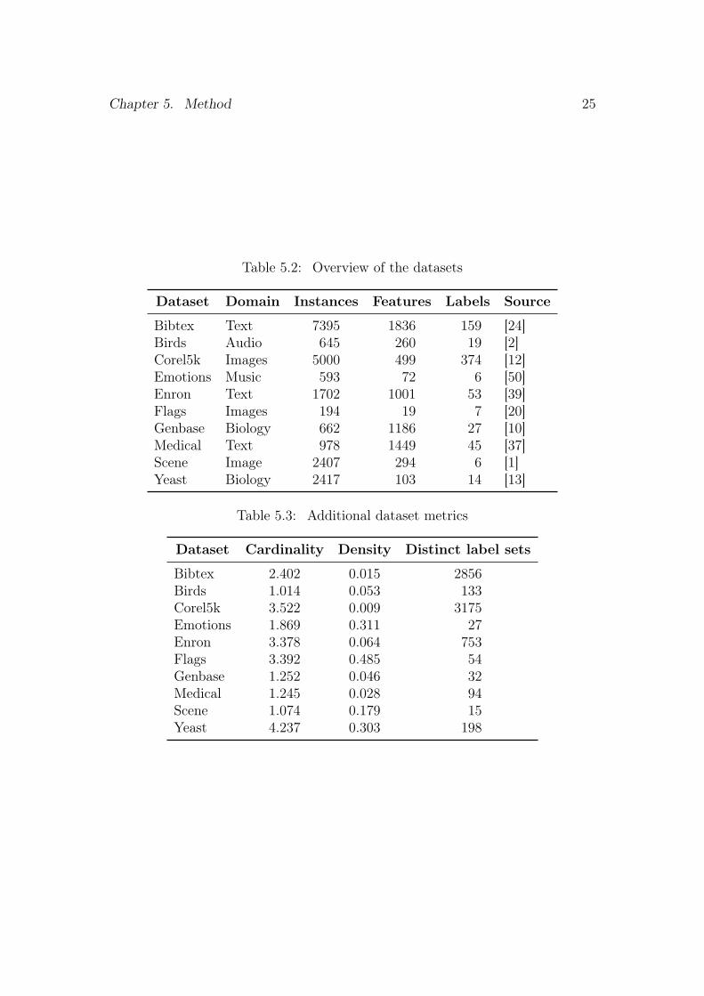
An overview of the datasets is presented in table 5.2, with additional infor-mation in table 5.3. Three multi-label dataset metrics are shown in table 5.3:cardinality, the average number of labels per instance [49]; density, the cardinal-ity divided by the number of labels [49]; and distinct label sets, the number ofunique label combinations observed in the dataset [58].

All datasets used in the experiment were acquired from the KDIS ResearchGroup’s collection1.

1http://www.uco.es/grupos/kdis/kdiswiki/index.php/Resources, 2017-02-09

http://www.uco.es/grupos/kdis/kdiswiki/index.php/Resources


Table 5.2: Overview of the datasets

Dataset Domain Instances Features Labels Source

Bibtex Text 7395 1836 159 [24]Birds Audio 645 260 19 [2]Corel5k Images 5000 499 374 [12]Emotions Music 593 72 6 [50]Enron Text 1702 1001 53 [39]Flags Images 194 19 7 [20]Genbase Biology 662 1186 27 [10]Medical Text 978 1449 45 [37]Scene Image 2407 294 6 [1]Yeast Biology 2417 103 14 [13]

Table 5.3: Additional dataset metrics

Dataset Cardinality Density Distinct label sets

Bibtex 2.402 0.015 2856Birds 1.014 0.053 133Corel5k 3.522 0.009 3175Emotions 1.869 0.311 27Enron 3.378 0.064 753Flags 3.392 0.485 54Genbase 1.252 0.046 32Medical 1.245 0.028 94Scene 1.074 0.179 15Yeast 4.237 0.303 198


5.3 MeasurementsClassification performance was evaluated using three different measures: accu-racy, 0/1 subset accuracy and Hamming loss. For a description of the measures,see section 3.1.2. In addition to the performance measures, the number of trueand false positive and negative labels were recorded.

Execution time was measured in the highest resolution offered by the JavaVirtual Machine and rounded to millisecond precision. The execution was dividedinto three stages for the purpose of runtime measurement. The first measurementcovered the chain selection stage, i.e. the preparatory step where FOCS or BOCSis used. The second measurement covered the classifier training stage, and thethird covered the classifier testing stage.

Both performance and execution time was measured separately for each of theten folds of every dataset. The measurements were then combined across folds toget the mean value and standard deviation for the dataset as a whole.

Chapter 6Results

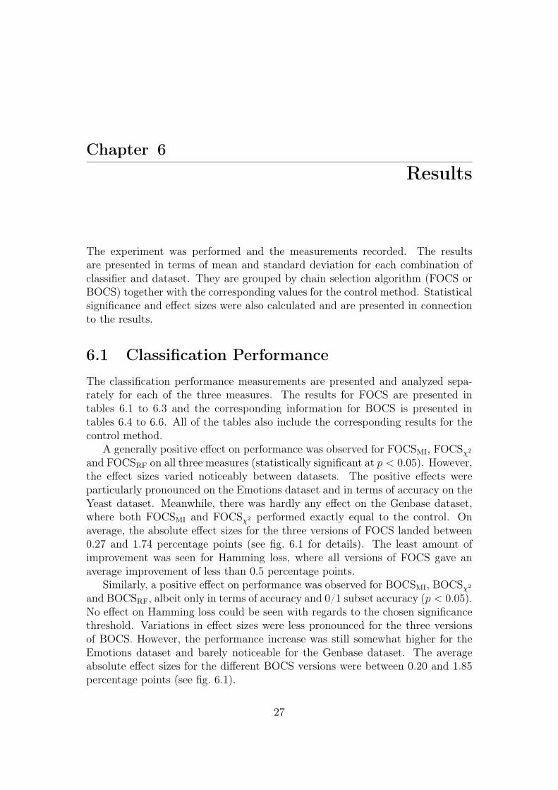
The experiment was performed and the measurements recorded. The resultsare presented in terms of mean and standard deviation for each combination ofclassifier and dataset. They are grouped by chain selection algorithm (FOCS orBOCS) together with the corresponding values for the control method. Statisticalsignificance and effect sizes were also calculated and are presented in connectionto the results.

6.1 Classification PerformanceThe classification performance measurements are presented and analyzed sepa-rately for each of the three measures. The results for FOCS are presented intables 6.1 to 6.3 and the corresponding information for BOCS is presented intables 6.4 to 6.6. All of the tables also include the corresponding results for thecontrol method.

A generally positive effect on performance was observed for FOCSMI, FOCSχ2

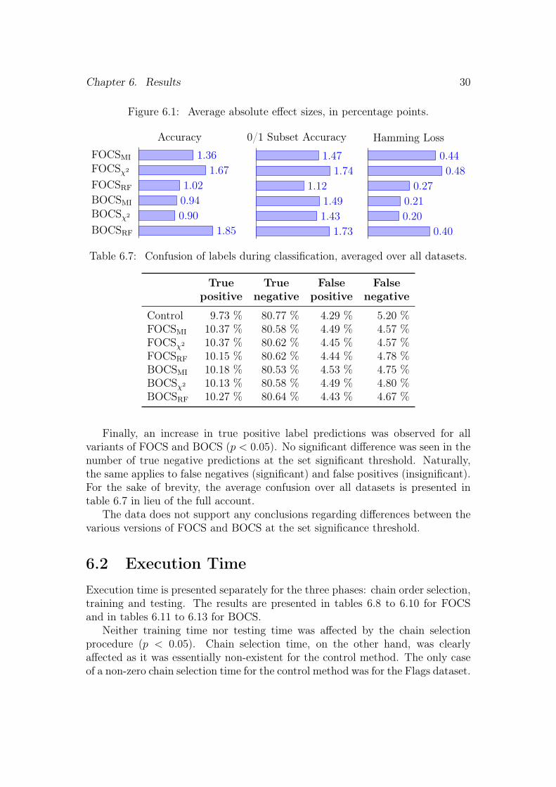
and FOCSRF on all three measures (statistically significant at p < 0.05). However,the effect sizes varied noticeably between datasets. The positive effects wereparticularly pronounced on the Emotions dataset and in terms of accuracy on theYeast dataset. Meanwhile, there was hardly any effect on the Genbase dataset,where both FOCSMI and FOCSχ2 performed exactly equal to the control. Onaverage, the absolute effect sizes for the three versions of FOCS landed between0.27 and 1.74 percentage points (see fig. 6.1 for details). The least amount ofimprovement was seen for Hamming loss, where all versions of FOCS gave anaverage improvement of less than 0.5 percentage points.

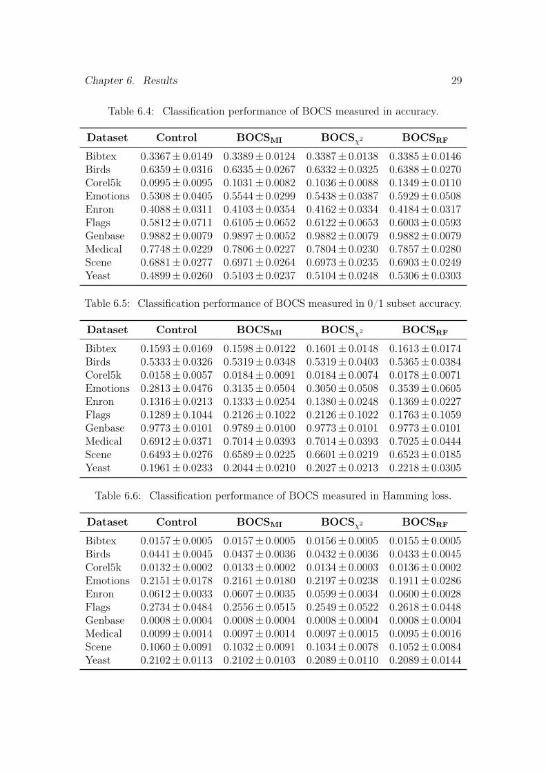
Similarly, a positive effect on performance was observed for BOCSMI, BOCSχ2

and BOCSRF, albeit only in terms of accuracy and 0/1 subset accuracy (p < 0.05).No effect on Hamming loss could be seen with regards to the chosen significancethreshold. Variations in effect sizes were less pronounced for the three versionsof BOCS. However, the performance increase was still somewhat higher for theEmotions dataset and barely noticeable for the Genbase dataset. The averageabsolute effect sizes for the different BOCS versions were between 0.20 and 1.85percentage points (see fig. 6.1).

27

Chapter 6. Results 28

Table 6.1: Classification performance of FOCS measured in accuracy.

Dataset Control FOCSMI FOCSχ2 FOCSRF

Bibtex 0.3367± 0.0149 0.3385± 0.0131 0.3386± 0.0121 0.3386± 0.0130Birds 0.6359± 0.0316 0.6432± 0.0347 0.6434± 0.0333 0.6367± 0.0319Corel5k 0.0995± 0.0095 0.0971± 0.0060 0.1143± 0.0097 0.0942± 0.0093Emotions 0.5308± 0.0405 0.5896± 0.0304 0.5914± 0.0495 0.5865± 0.0414Enron 0.4088± 0.0311 0.4100± 0.0343 0.4098± 0.0368 0.4117± 0.0369Flags 0.5812± 0.0711 0.6069± 0.0746 0.6129± 0.0776 0.5824± 0.0620Genbase 0.9882± 0.0079 0.9882± 0.0079 0.9882± 0.0079 0.9897± 0.0052Medical 0.7748± 0.0229 0.7780± 0.0249 0.7789± 0.0233 0.7789± 0.0269Scene 0.6881± 0.0277 0.6912± 0.0227 0.6934± 0.0272 0.6966± 0.0296Yeast 0.4899± 0.0260 0.5270± 0.0289 0.5303± 0.0289 0.5204± 0.0223

Table 6.2: Classification performance of FOCS measured in 0/1 subset accuracy.



Table 6.3: Classification performance of FOCS measured in Hamming loss.




Table 6.4: Classification performance of BOCS measured in accuracy.

Dataset Control BOCSMI BOCSχ2 BOCSRF


Table 6.5: Classification performance of BOCS measured in 0/1 subset accuracy.



Table 6.6: Classification performance of BOCS measured in Hamming loss.




Figure 6.1: Average absolute effect sizes, in percentage points.

BOCSRF

BOCSχ2

BOCSMI

FOCSRF

FOCSχ2

FOCSMI 1.36

1.67

1.02

0.94

0.90

1.85

Accuracy

1.47

1.74

1.12

1.49

1.43

1.73

0/1 Subset Accuracy

0.44

0.48

0.27

0.21

0.20

0.40

Hamming Loss

Table 6.7: Confusion of labels during classification, averaged over all datasets.

True True False Falsepositive negative positive negative

Control 9.73 % 80.77 % 4.29 % 5.20 %FOCSMI 10.37 % 80.58 % 4.49 % 4.57 %FOCSχ2 10.37 % 80.62 % 4.45 % 4.57 %FOCSRF 10.15 % 80.62 % 4.44 % 4.78 %BOCSMI 10.18 % 80.53 % 4.53 % 4.75 %BOCSχ2 10.13 % 80.58 % 4.49 % 4.80 %BOCSRF 10.27 % 80.64 % 4.43 % 4.67 %

Finally, an increase in true positive label predictions was observed for allvariants of FOCS and BOCS (p < 0.05). No significant difference was seen in thenumber of true negative predictions at the set significant threshold. Naturally,the same applies to false negatives (significant) and false positives (insignificant).For the sake of brevity, the average confusion over all datasets is presented intable 6.7 in lieu of the full account.

The data does not support any conclusions regarding differences between thevarious versions of FOCS and BOCS at the set significance threshold.

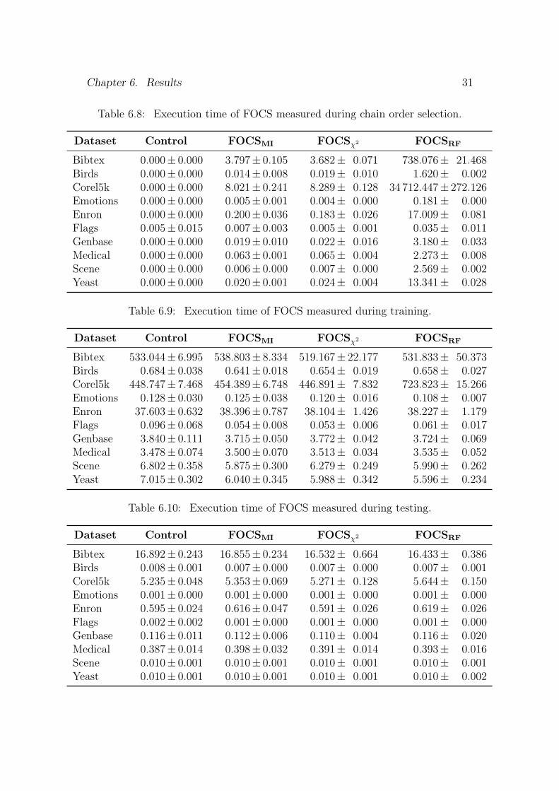
6.2 Execution TimeExecution time is presented separately for the three phases: chain order selection,training and testing. The results are presented in tables 6.8 to 6.10 for FOCSand in tables 6.11 to 6.13 for BOCS.

Neither training time nor testing time was affected by the chain selectionprocedure (p < 0.05). Chain selection time, on the other hand, was clearlyaffected as it was essentially non-existent for the control method. The only caseof a non-zero chain selection time for the control method was for the Flags dataset.


Table 6.8: Execution time of FOCS measured during chain order selection.


Bibtex 0.000± 0.000 3.797± 0.105 3.682± 0.071 738.076± 21.468Birds 0.000± 0.000 0.014± 0.008 0.019± 0.010 1.620± 0.002Corel5k 0.000± 0.000 8.021± 0.241 8.289± 0.128 34 712.447± 272.126Emotions 0.000± 0.000 0.005± 0.001 0.004± 0.000 0.181± 0.000Enron 0.000± 0.000 0.200± 0.036 0.183± 0.026 17.009± 0.081Flags 0.005± 0.015 0.007± 0.003 0.005± 0.001 0.035± 0.011Genbase 0.000± 0.000 0.019± 0.010 0.022± 0.016 3.180± 0.033Medical 0.000± 0.000 0.063± 0.001 0.065± 0.004 2.273± 0.008Scene 0.000± 0.000 0.006± 0.000 0.007± 0.000 2.569± 0.002Yeast 0.000± 0.000 0.020± 0.001 0.024± 0.004 13.341± 0.028

Table 6.9: Execution time of FOCS measured during training.



Table 6.10: Execution time of FOCS measured during testing.




Table 6.11: Execution time of BOCS measured during chain order selection.


Bibtex 0.000± 0.000 4.829± 0.091 4.760± 0.097 578.059± 4.146Birds 0.000± 0.000 0.012± 0.004 0.010± 0.001 1.694± 0.005Corel5k 0.000± 0.000 8.781± 0.292 8.023± 0.134 28 166.410± 193.356Emotions 0.000± 0.000 0.005± 0.001 0.005± 0.000 0.200± 0.000Enron 0.000± 0.000 0.183± 0.002 0.187± 0.012 17.144± 0.071Flags 0.005± 0.015 0.014± 0.010 0.017± 0.016 0.038± 0.010Genbase 0.000± 0.000 0.026± 0.001 0.030± 0.006 3.721± 0.060Medical 0.000± 0.000 0.094± 0.041 0.094± 0.028 2.217± 0.018Scene 0.000± 0.000 0.009± 0.000 0.009± 0.000 2.991± 0.023Yeast 0.000± 0.000 0.031± 0.004 0.031± 0.004 15.405± 0.316

Table 6.12: Execution time of BOCS measured during training.


Bibtex 533.044± 6.995 557.585±26.168 514.067± 5.418 466.410± 4.309Birds 0.684± 0.038 0.718± 0.034 0.693± 0.045 0.917± 0.047Corel5k 448.747± 7.468 470.804±24.293 468.061± 6.087 587.266± 24.330Emotions 0.128± 0.030 0.161± 0.065 0.139± 0.037 0.130± 0.007Enron 37.603± 0.632 41.313± 1.516 38.474± 0.931 39.424± 1.982Flags 0.096± 0.068 0.088± 0.057 0.086± 0.062 0.064± 0.011Genbase 3.840± 0.111 6.533± 0.113 6.591± 0.219 6.648± 0.149Medical 3.478± 0.074 3.675± 0.189 3.684± 0.124 3.541± 0.069Scene 6.802± 0.358 6.499± 0.272 6.257± 0.256 5.983± 0.236Yeast 7.015± 0.302 6.935± 0.345 6.640± 0.259 7.541± 0.852

Table 6.13: Execution time of BOCS measured during testing.




A particularly notable aspect is the magnitude of the selection time measure-ments for both ReliefF-based versions, FOCSRF and BOCSRF. Especially on thelargest dataset, Corel5k.

Effect sizes are omitted due to the nature of the data. It was deemed redun-dant for the insignificant differences in training and testing times and superfluousfor the chain selection times (the absolute effect size is equal to the mean valuewhen the control group’s mean value is zero).

Chapter 7Analysis and Discussion

The study’s results are analyzed and discussed in order to answer the posedresearch questions.

The first and second research questions regard the method for algorithm adap-tation and chain ordering. They are answered through the formulation of theproposed approach in chapter 4. The proposed approach is founded upon theadaptation of filter model feature selection techniques to evaluate label depen-dencies, giving the answer to the first question. Two answers are given in responseto the second question: the forward-oriented and the backward-oriented chain or-dering methods used in FOCS and BOCS, respectively.

The third and fourth research questions focus on the proposed approach’simpact on the Classifier Chain. These questions will be answered by analyzingthe measurements acquired through the experiment.

7.1 Classification PerformanceAll versions of both FOCS and BOCS improved the classification performance.However, the amount of improvement varied for the different measures.

Nearly all versions of FOCS and BOCS (BOCSRF being the exception) im-proved the most in terms of 0/1 subset accuracy. The Classifier Chain is itselffocused on maximizing the 0/1 subset accuracy (or, equivalently, on minimizingthe 0/1 loss) [8]. Thus, improvement with regards to this measure is arguably ofparticular importance. Improving the classifier’s primary strength increases itsusefulness for its most suitable applications. With 0/1 subset accuracy being themost concerned with the multi-label problem as a whole, the improved resultsalso hint at the techniques’ success in exploiting label dependence.

At the same time, no version of BOCS showed any significant effect on Ham-ming loss. Even for FOCS, where a significant positive effect was observed, theeffect was noticeably lower than for the other measures. The low impact on Ham-ming loss mirrors the Classifier Chain’s own performance profile and is somewhatunsurprising, since Hamming loss can be optimized by disregarding label depen-dencies [41]. However, the contrast between the 0/1 subset accuracy and the

34

Chapter 7. Analysis and Discussion 35

Hamming loss scores seems to reveal an interesting aspect of both chain orderingtechniques, namely an increased propensity for error propagation.

The Classifier Chain’s exploitation of label dependence helps to correctly pre-dict labels, as long as the previous labels in the chain were correctly predicted.When a label is misclassified, however, the error may propagate throughout thechain and cause additional mistakes [8, 41].

The positive effects of exploiting label dependence are amplified by the pro-posed algorithms, as they select chain orders specifically to facilitate the labels’influence on each other. Consequently, a Classifier Chain ordered using FOCSor BOCS is able to better exploit the dependencies between labels to achievea higher number of perfectly predicted label sets (a higher score for 0/1 subsetaccuracy). Intuitively, this ought to entail an improvement for other performancemeasures such as Hamming loss, too, as it would mean a greater total numberof correctly predicted labels. The fact that the Hamming loss does not improveas much may imply an amplification of the error propagation as well. That is,the increase in perfectly predicted label sets is partially compensated for by anincreased number of erroneous predictions for instances where some label hasalready been misclassified. Essentially, a Classifier Chain ordered by FOCS orBOCS is better at making perfect classifications, but makes more mistakes onpartially correct classifications. Do keep in mind, though, that the Hamming losswas not affected negatively by the use of either algorithm. The net result is stillpositive (FOCS) or neutral (BOCS) in terms of Hamming loss.

Looking at the methods’ impact on true and false positive label predictionsreveals further information about their effects. All variants of both FOCS andBOCS increased the number of true positive predictions. This means that theordered Classifier Chains are better at correctly assigning the expected labels toinstances. However, the number of false positives also appears to increase slightly,albeit less than the true positives. In fact, this (possible) increase was too smallto be ruled statistically significant at p < 0.05. Nonetheless it is a potentialdrawback and should perhaps not be entirely disregarded.

An increase in both true and false positives would match the previous discus-sion on error propagation. By amplifying the exploitation of label dependence,the classifier may perceive stronger evidence for the inclusion of certain labels.Oftentimes this is desirable, as evident from the increase in true positives, while atother times it is not. The classifier appears to be more confident when assigninglabels, possibly even at times when it ought not to be. Such an effect would beconsistent with the Classifier Chain’s eagerness to find label dependencies, evenwhen there are none [8].

Another, unrelated observation is the notable difference in effect sizes betweensome of the datasets. The performance on the Genbase dataset was barely affectedby the change in chain order, while the performance on the Emotions dataset washeavily affected. This is possibly just an effect of different datasets containingvarious levels of label dependence. Although a purely speculative explanation,


it appears consistent with results from related work, where the performance onGenbase was completely unaffected by both the chain order and the considerationof label dependence in general [20, 41].

Finally, there is the aspect of marginal versus conditional label dependence.The dependency calculations in FOCS and BOCS estimate the marginal labeldependence. Meanwhile, the Classifier Chain inherently models conditional labeldependence [8]. It is unclear how, or if, this contrariety affects the performance.However, the effect is speculated to be slight as the two types of dependence areoften (though not always) closely related. It has also been shown to have littleimpact on the related Bayesian Classifier Chain [42], leading to the belief thatthe same may be true for the regular Classifier Chain.

The effect sizes achieved by FOCS and BOCS appear roughly comparable tothose achieved by similar methods [20, 26, 38]. However, a rigorous comparisonis hindered by disparities between the various studies. In fact, only one of themethods has even been evaluated on the original Classifier Chain algorithm [20].In that case, the improvements are close enough to FOCS and BOCS to be deemedstatistically insignificant (Friedman test, significance threshold 0.05).

Generally, the results support the existing consensus that chain order matters.Similar to previous studies, the classification performance was shown to improvewith a more meticulous approach to chain ordering. Furthermore, the proposedmethod’s success supports the notion that measure-/metrics-based approaches isa viable way to tackle the chain ordering problem.

7.2 Execution TimeThe use of FOCS or BOCS did not significantly affect the training time nor thetesting time. This was expected and is entirely unsurprising, as neither algorithmalters the Classifier Chain’s procedure for training or inference. Instead, the fullimpact on execution time was contained in what was dubbed the chain orderselection phase.

Note that chain order selection is technically part of the training step, thoughit is prepended to, and thus precedes, the regular training procedure. It is keptseparate here for the sole purpose of improved clarity, by isolating the proposedapproach’s impact. The time spent on chain selection should be added to thetraining time if compared to other studies or classifiers where such a distinctionis not made.

The chain selection phase is essentially non-existent in the usual, implicitlyordered Classifier Chain. In such a case, the order does not need to be calculated.Instead, it is always as defined in the dataset, i.e. {y1 → y2 → · · · → yL}. It isthus surprising that the control method measured a non-zero value for the Birdsdataset.

The generally low impact on execution time gives substance to the assumption


Figure 7.1: Increases in execution time compared to the control method.

BOCSRF

BOCSχ2

BOCSMI

FOCSRF

FOCSχ2

FOCSMI 1.8 %1.7 %

860.0 %2.6 %2.9 %

720.5 %

Average

1.8 %1.8 %

7,646.2 %1.9 %1.8 %

6,204.3 %

Corel5k

that filter model feature selection techniques can be efficiently applied to thechain ordering problem. The versions of both FOCS and BOCS which are basedon mutual information and the χ2 statistic showed similar execution times andscaled very well with the dataset size. However, the two ReliefF-based versionswere considerably more costly in all observed cases and scaled markedly worse.

To put the cost in perspective, consider the time spent on chain order selectionin relation to the time it takes to train and test a single Classifier Chain (fig. 7.1).On average, FOCSχ2 increased the execution time by only 1.7 %, FOCSMI by1.8 %, BOCSMI by 2.6 % and BOCSχ2 by 2.9 %. BOCSRF, on the other hand,increased the runtime by an average of 720 % and FOCSRF by 860 %. Consideringonly the largest dataset, Corel5k, the mutual information- and χ2-based versionsall increased the runtime by only 1.8 % to 1.9 %. Meanwhile, the ReliefF-basedversions of FOCS and BOCS increased the runtime by approximately 7650 %and 6200 %, respectively. The great difference in execution time accentuates thefeature evaluator’s influence over FOCS and BOCS, even though no significantdifference in classification performance was observed for the different evaluators.

The high computational cost of the ReliefF-based versions compared to theothers effectively rules out FOCSRF and BOCSRF as viable alternatives, at leastfor large datasets. As the high cost stems from ReliefF rather than from FOCSor BOCS themselves, a deeper discussion of it is beyond the scope of this study.However, it should be noted that the computational cost of ReliefF is greatlyaffected by its parameters, including both the number of sampled instances andthe number of sampled neighbors per instance. It is thus plausible that some otherconfiguration would have provided more favorable execution times. Verifying thissimilarly falls outside of the study’s scope.

Compared to other chain selection techniques, FOCSMI, FOCSχ2 , BOCSMI

and BOCSχ2 are all very competitive in terms of computational cost. In fact,even FOCSRF and BOCSRF are moderately cheap compared to some of the pre-existing alternatives. While the former four add a few percent to the executiontime, other methods typically cause multiplicative increases as a consequence oftrying out a large number of chains. Reports on actual execution times are unfor-


tunately scarce in the related literature, prohibiting a direct comparison to mostalternatives. The only available example is for the Monte Carlo approach, whichadds between 4500 % and 41 000 % to the training time [38]. However, both thegenetic algorithm approach [20] and one of the beam search-based techniques [26]evaluate large numbers of chains, reasonably leading to a manifold increase inexecution time as well. Meanwhile, the mutual information- and χ2-based ver-sions of FOCS and BOCS are far cheaper than the evaluation of even a singleadditional chain.

The low computational cost is a compelling argument in favor of metrics-basedapproaches to chain ordering. It demonstrates their main advantage over directevaluation of multiple chains. Previous studies have discussed similar advantagesin the context of related algorithms [27, 42]. The results for FOCS and BOCSthus adds evidence in support of this idea, while simultaneously showing thatthe same is true for the Classifier Chain algorithm. With these results and theprevious studies’ observations in mind, it may be more worthwhile to focus futureefforts on techniques that do not rely on trying out numerous chains.

7.3 Validity Threats and LimitationsMost threats to the study’s validity were offset by careful consideration for theexperiment’s design and the statistical verification of the results. Nonetheless,not all validity threats could be completely eliminated.

A remaining threat to the internal validity regards the accuracy of the ex-ecution time measurements. The experiment ran on a shared system alongsideother applications, meaning that variations caused by resource contention andjob scheduling are likely to have influenced the results. All time measurementswere averaged across ten runs specifically in an attempt to reduce the impactof such sporadic events. Furthermore, the experiment was implemented in Javaand is thus subject to Java’s JIT compilation and optimization. This may alsohave affected the execution times. One instance of such interference is believedto have caused the abnormality in the control method’s chain selection time onthe Flags dataset. The first such test (out of ten) occurs at the very beginningof the experiment and takes markedly longer than the others.

As for the external validity, the dataset selection holds another potentialthreat. The datasets were chosen to make up a varied and representative col-lection. However, the selection may be biased in terms of some unconsideredaspect, which could then have impacted the results.

On a separate note, the study is limited by its inability to draw any con-clusions regarding the relative performances of the proposed algorithms. Theresults supported conclusions regarding both algorithms’ superiority to the con-trol method. However, the results were inconclusive regarding any differencesbetween FOCSMI, FOCSχ2 , FOCSRF, BOCSMI, BOCSχ2 and BOCSRF, It seems


intuitively unlikely that all six variants are equally well-performing. Differencesin ranks and effect sizes appear to suggest that there is some difference, as well.Nonetheless, the differences are too small to allow for any such conclusions with-out a high risk of type I or family-wise errors. A larger number of samples (i.e.additional datasets) could possibly have allowed for such comparisons.

Another limitation is the lack of rigorous comparison to other methods fromrelated literature. This is caused by two separate issues. Firstly, the body ofpreviously published work does not contain the necessary information to directlycompare results across those studies. The diversity in used datasets, measuresand classifiers means there is very little common ground between the experiments.Secondly, a shortage of available implementations hinders the use of the pre-existing methods. As a consequence, they could not be included in the performedexperiment, either. Creating and verifying new implementations of the othermethods would require a great deal of additional work and was not feasible withinthe confines of this study.

Chapter 8Conclusions and Future Work

This study proposes a novel approach to estimate label dependencies in multi-label data. The label dependence evaluation problem is transformed into multiplefeature evaluation problems. Off-the-shelf feature evaluators are then used toestimate the label dependence. Two algorithms based on this approach, FOCSand BOCS, were also proposed to exploit such knowledge when constructingClassifier Chains.

An experiment was performed to assess the proposed approach. The proposedalgorithms were evaluated with three different feature evaluators. The resultswere compared to the typical case of an implicitly ordered Classifier Chain.

Improvements were observed in terms of accuracy and 0/1 subset accuracyfor both algorithms. FOCS additionally showed significant improvement in termsof Hamming loss, while BOCS did not. Execution time measurements showedan increased computational cost of only a few percent in most cases. The pro-posed approach was thus shown to be an improvement over the typical approachto Classifier Chain construction. Additionally, the performance improvementsappeared similar in magnitude to those reported for comparable techniques inrelated work, but at a highly competitive computational cost.

The results substantiate the presupposition that filter model feature selectiontechniques can be applied to Classifier Chain ordering. They furthermore demon-strate the viability of the approach and establish both FOCS and BOCS as strongalternatives worthy of further consideration.

The novel algorithms for Classifier Chain ordering is the primary contributionof this study. By improving the classifier’s performance at a low cost, the pro-posed techniques are potentially useful to anyone working with Classifier Chains.Simultaneously, the study details a new and cost-effective way to evaluate labeldependence in multi-label data. This technique has other potential applicationswithin multi-label classification. It may thus be of interest in itself to researchersdeveloping other types of classifiers for multi-label classification.

In future work, a comparison of different versions of FOCS and BOCS shouldbe performed. Knowing more about their relative performance and the effects ofdifferent feature evaluators would be useful for future applications. Similarly, a re-evaluation of existing chain ordering techniques under equal conditions would also

40

Chapter 8. Conclusions and Future Work 41

be highly beneficial to future research and would fill a gap in current literature.Existing evaluations have all been performed in very different settings, hinderingfair comparison.

Another interesting line of research would be to apply the proposed approachto build other types of classifier structures, e.g. partially connected chains orClassifier Trellises. Finally, a last suggestion would be to extend the proposedevaluation technique to estimate conditional label dependence and to investigatehow that affects the performance and cost.

References

[1] Matthew R. Boutell et al. “Learning multi-label scene classification”. In:Pattern Recognition 37.9 (2004), pp. 1757–1771. doi: 10.1016/j.patcog.2004.03.009. url: https://doi.org/10.1016/j.patcog.2004.03.009.

[2] Forrest Briggs et al. “The 9th annual MLSP competition: New methodsfor acoustic classification of multiple simultaneous bird species in a noisyenvironment”. In: IEEE International Workshop on Machine Learning forSignal Processing, MLSP 2013, Southampton, United Kingdom, September22-25, 2013. IEEE, 2013, pp. 1–8. doi: 10.1109/MLSP.2013.6661934. url:https://doi.org/10.1109/MLSP.2013.6661934.

[3] Klaus Brinker, Johannes Fürnkranz, and Eyke Hüllermeier. “A UnifiedModel for Multilabel Classification and Ranking”. In: ECAI 2006, 17thEuropean Conference on Artificial Intelligence, August 29 - September 1,2006, Riva del Garda, Italy, Including Prestigious Applications of Intel-ligent Systems (PAIS 2006), Proceedings. Ed. by Gerhard Brewka et al.Vol. 141. Frontiers in Artificial Intelligence and Applications. IOS Press,2006, pp. 489–493. isbn: 1-58603-642-4.

[4] Benhui Chen et al. “Enhancing multi-label classification based on local labelconstraints and classifier chains”. In: 2016 International Joint Conference onNeural Networks, IJCNN 2016, Vancouver, BC, Canada, July 24-29, 2016.IEEE, 2016, pp. 1458–1463. isbn: 978-1-5090-0620-5. doi: 10.1109/IJCNN.2016.7727370. url: http://dx.doi.org/10.1109/IJCNN.2016.7727370.

[5] Thomas M. Cover and Joy A. Thomas. Elements of information theory (2.ed.) Wiley, 2006. isbn: 978-0-471-24195-9.

[6] Krzysztof Dembczynski, Weiwei Cheng, and Eyke Hüllermeier. “BayesOptimal Multilabel Classification via Probabilistic Classifier Chains”. In:Proceedings of the 27th International Conference on Machine Learning(ICML-10), June 21-24, 2010, Haifa, Israel. Ed. by Johannes Fürnkranzand Thorsten Joachims. Omnipress, 2010, pp. 279–286. url: http://www.icml2010.org/papers/589.pdf.

42

http://dx.doi.org/10.1016/j.patcog.2004.03.009


https://doi.org/10.1016/j.patcog.2004.03.009

http://dx.doi.org/10.1109/MLSP.2013.6661934

https://doi.org/10.1109/MLSP.2013.6661934

http://dx.doi.org/10.1109/IJCNN.2016.7727370



http://www.icml2010.org/papers/589.pdf

http://www.icml2010.org/papers/589.pdf

REFERENCES 43

[7] Krzysztof Dembczynski, Willem Waegeman, and Eyke Hüllermeier. “AnAnalysis of Chaining in Multi-Label Classification”. In: ECAI 2012 - 20thEuropean Conference on Artificial Intelligence. Including Prestigious Ap-plications of Artificial Intelligence (PAIS-2012) System DemonstrationsTrack, Montpellier, France, August 27-31 , 2012. Ed. by Luc De Raedtet al. Vol. 242. Frontiers in Artificial Intelligence and Applications. IOSPress, 2012, pp. 294–299. isbn: 978-1-61499-097-0. doi: 10.3233/978-1-61499-098-7-294. url: http://dx.doi.org/10.3233/978-1-61499-098-7-294.

[8] Krzysztof Dembczynski et al. “On label dependence and loss minimizationin multi-label classification”. In: Machine Learning 88.1-2 (2012), pp. 5–45.doi: 10.1007/s10994-012-5285-8. url: http://dx.doi.org/10.1007/s10994-012-5285-8.

[9] Janez Demsar. “Statistical Comparisons of Classifiers over Multiple DataSets”. In: Journal of Machine Learning Research 7 (2006), pp. 1–30. url:http://www.jmlr.org/papers/v7/demsar06a.html.

[10] Sotiris Diplaris et al. “Protein Classification with Multiple Algorithms”. In:Advances in Informatics, 10th Panhellenic Conference on Informatics, PCI2005, Volos, Greece, November 11-13, 2005, Proceedings. Ed. by PanayiotisBozanis and Elias N. Houstis. Vol. 3746. Lecture Notes in Computer Science.Springer, 2005, pp. 448–456. isbn: 3-540-29673-5. doi: 10.1007/11573036_42. url: https://doi.org/10.1007/11573036_42.

[11] Gauthier Doquire and Michel Verleysen. “Feature Selection for Multi-labelClassification Problems”. In: Advances in Computational Intelligence - 11thInternational Work-Conference on Artificial Neural Networks, IWANN2011, Torremolinos-Málaga, Spain, June 8-10, 2011, Proceedings, PartI. Ed. by Joan Cabestany, Ignacio Rojas, and Gonzalo Joya Caparrós.Vol. 6691. Lecture Notes in Computer Science. Springer, 2011, pp. 9–16.isbn: 978-3-642-21500-1. doi: 10.1007/978- 3- 642- 21501- 8_2. url:http://dx.doi.org/10.1007/978-3-642-21501-8_2.

[12] Pinar Duygulu et al. “Object Recognition as Machine Translation: Learn-ing a Lexicon for a Fixed Image Vocabulary”. In: Computer Vision - ECCV2002, 7th European Conference on Computer Vision, Copenhagen, Den-mark, May 28-31, 2002, Proceedings, Part IV. Ed. by Anders Heyden etal. Vol. 2353. Lecture Notes in Computer Science. Springer, 2002, pp. 97–112. isbn: 3-540-43748-7. doi: 10.1007/3-540-47979-1_7. url: https://doi.org/10.1007/3-540-47979-1_7.

[13] André Elisseeff and Jason Weston. “A kernel method for multi-labelled clas-sification”. In: Advances in Neural Information Processing Systems 14 [Neu-ral Information Processing Systems: Natural and Synthetic, NIPS 2001, De-cember 3-8, 2001, Vancouver, British Columbia, Canada]. Ed. by Thomas

http://dx.doi.org/10.3233/978-1-61499-098-7-294

http://dx.doi.org/10.3233/978-1-61499-098-7-294

http://dx.doi.org/10.3233/978-1-61499-098-7-294

http://dx.doi.org/10.3233/978-1-61499-098-7-294

http://dx.doi.org/10.1007/s10994-012-5285-8

http://dx.doi.org/10.1007/s10994-012-5285-8

http://dx.doi.org/10.1007/s10994-012-5285-8

http://www.jmlr.org/papers/v7/demsar06a.html

http://dx.doi.org/10.1007/11573036_42

http://dx.doi.org/10.1007/11573036_42

https://doi.org/10.1007/11573036_42

http://dx.doi.org/10.1007/978-3-642-21501-8_2

http://dx.doi.org/10.1007/978-3-642-21501-8_2

http://dx.doi.org/10.1007/3-540-47979-1_7

https://doi.org/10.1007/3-540-47979-1_7

https://doi.org/10.1007/3-540-47979-1_7

REFERENCES 44

G. Dietterich, Suzanna Becker, and Zoubin Ghahramani. MIT Press, 2001,pp. 681–687. url: http://papers.nips.cc/paper/1964-a-kernel-method-for-multi-labelled-classification.

[14] Peter Flach. Machine Learning: The Art and Science of Algorithms thatMake Sense of Data. Cambridge University Press, 2012. isbn: 9781107422223.

[15] Eibe Frank, Mark A. Hall, and Ian H. Witten. The WEKA Workbench.4th ed. Online Appendix for Data Mining: Practical Machine Learning Toolsand Techniques. Morgan Kaufmann, 2016. url: http://www.cs.waikato.ac.nz/ml/weka/Witten_et_al_2016_appendix.pdf.

[16] Milton Friedman. “The Use of Ranks to Avoid the Assumption of NormalityImplicit in the Analysis of Variance”. In: Journal of the American StatisticalAssociation 32.200 (1937), pp. 675–701. issn: 01621459. doi: 10.2307/2279372. url: http://www.jstor.org/stable/2279372.

[17] Eva Gibaja and Sebastián Ventura. “A Tutorial on Multilabel Learning”.In: ACM Comput. Surv. 47.3 (2015), 52:1–52:38. doi: 10.1145/2716262.url: http://doi.acm.org/10.1145/2716262.

[18] Shantanu Godbole and Sunita Sarawagi. “Discriminative Methods forMulti-labeled Classification”. In: Advances in Knowledge Discovery andData Mining, 8th Pacific-Asia Conference, PAKDD 2004, Sydney, Aus-tralia, May 26-28, 2004, Proceedings. Ed. by Honghua Dai, RamakrishnanSrikant, and Chengqi Zhang. Vol. 3056. Lecture Notes in Computer Science.Springer, 2004, pp. 22–30. isbn: 3-540-22064-X. doi: 10.1007/978-3-540-24775-3_5. url: http://dx.doi.org/10.1007/978-3-540-24775-3_5.

[19] Anna Goldenberg and Andrew W. Moore. “Tractable learning of largeBayes net structures from sparse data”. In: Machine Learning, Proceedingsof the Twenty-first International Conference (ICML 2004), Banff, Alberta,Canada, July 4-8, 2004. Ed. by Carla E. Brodley. Vol. 69. ACM Interna-tional Conference Proceeding Series. ACM, 2004. doi: 10.1145/1015330.1015406. url: http://doi.acm.org/10.1145/1015330.1015406.

[20] Eduardo Corrêa Gonçalves, Alexandre Plastino, and Alex Alves Freitas.“A Genetic Algorithm for Optimizing the Label Ordering in Multi-labelClassifier Chains”. In: 2013 IEEE 25th International Conference on Toolswith Artificial Intelligence, Herndon, VA, USA, November 4-6, 2013. IEEEComputer Society, 2013, pp. 469–476. isbn: 978-1-4799-2971-9. doi: 10.1109/ICTAI.2013.76. url: http://dx.doi.org/10.1109/ICTAI.2013.76.

[21] Eduardo Corrêa Gonçalves, Alexandre Plastino, and Alex Alves Freitas.“Simpler is Better: a Novel Genetic Algorithm to Induce Compact Multi-label Chain Classifiers”. In: Proceedings of the Genetic and EvolutionaryComputation Conference, GECCO 2015, Madrid, Spain, July 11-15, 2015.

http://papers.nips.cc/paper/1964-a-kernel-method-for-multi-labelled-classification

http://papers.nips.cc/paper/1964-a-kernel-method-for-multi-labelled-classification

http://www.cs.waikato.ac.nz/ml/weka/Witten_et_al_2016_appendix.pdf

http://www.cs.waikato.ac.nz/ml/weka/Witten_et_al_2016_appendix.pdf

http://dx.doi.org/10.2307/2279372

http://dx.doi.org/10.2307/2279372

http://www.jstor.org/stable/2279372

http://dx.doi.org/10.1145/2716262

http://doi.acm.org/10.1145/2716262

http://dx.doi.org/10.1007/978-3-540-24775-3_5

http://dx.doi.org/10.1007/978-3-540-24775-3_5

http://dx.doi.org/10.1007/978-3-540-24775-3_5

http://dx.doi.org/10.1145/1015330.1015406

http://dx.doi.org/10.1145/1015330.1015406

http://doi.acm.org/10.1145/1015330.1015406

http://dx.doi.org/10.1109/ICTAI.2013.76




REFERENCES 45

Ed. by Sara Silva and Anna Isabel Esparcia-Alcázar. ACM, 2015, pp. 559–566. isbn: 978-1-4503-3472-3. doi: 10.1145/2739480.2754650. url: http://doi.acm.org/10.1145/2739480.2754650.

[22] Robin Gustafsson. Replication Data for: Ordering Classifier Chains usingfilter model feature selection techniques. 2017. doi: 10.7910/DVN/BA57IF.url: http://dx.doi.org/10.7910/DVN/BA57IF.

[23] Yosef Hochberg. “A sharper Bonferroni procedure for multiple tests of sig-nificance”. In: Biometrika 75.4 (1988), p. 800. doi: 10.1093/biomet/75.4.800. eprint: /oup/backfile/Content_public/Journal/biomet/75/4/10.1093/biomet/75.4.800/2/75-4-800.pdf. url: http://dx.doi.org/10.1093/biomet/75.4.800.

[24] Ioannis Katakis, Grigorios Tsoumakas, and Ioannis Vlahavas. “MultilabelText Classification for Automated Tag Suggestion”. In: Proceedings of theECML/PKDD 2008 Discovery Challenge. Antwerp, Belgium, 2008.

[25] Igor Kononenko. “Estimating Attributes: Analysis and Extensions of RE-LIEF”. In: Machine Learning: ECML-94, European Conference on MachineLearning, Catania, Italy, April 6-8, 1994, Proceedings. Ed. by FrancescoBergadano and Luc De Raedt. Vol. 784. Lecture Notes in Computer Sci-ence. Springer, 1994, pp. 171–182. isbn: 3-540-57868-4. doi: 10.1007/3-540-57868-4_57. url: http://dx.doi.org/10.1007/3-540-57868-4_57.

[26] Abhishek Kumar et al. “Beam search algorithms for multilabel learning”.In: Machine Learning 92.1 (2013), pp. 65–89. doi: 10.1007/s10994-013-5371-6. url: http://dx.doi.org/10.1007/s10994-013-5371-6.

[27] Abhishek Kumar et al. “Learning and Inference in Probabilistic ClassifierChains with Beam Search”. In: Machine Learning and Knowledge Discov-ery in Databases - European Conference, ECML PKDD 2012, Bristol, UK,September 24-28, 2012. Proceedings, Part I. Ed. by Peter A. Flach, Tijl DeBie, and Nello Cristianini. Vol. 7523. Lecture Notes in Computer Science.Springer, 2012, pp. 665–680. isbn: 978-3-642-33459-7. doi: 10.1007/978-3-642-33460-3_48. url: http://dx.doi.org/10.1007/978-3-642-33460-3_48.

[28] Jaedong Lee et al. “An approach for multi-label classification by directedacyclic graph with label correlation maximization”. In: Inf. Sci. 351 (2016),pp. 101–114. doi: 10.1016/j.ins.2016.02.037. url: http://dx.doi.org/10.1016/j.ins.2016.02.037.

[29] Nan Li and Zhi-Hua Zhou. “Selective Ensemble of Classifier Chains”. In:Multiple Classifier Systems, 11th International Workshop, MCS 2013, Nan-jing, China, May 15-17, 2013. Proceedings. Ed. by Zhi-Hua Zhou, FabioRoli, and Josef Kittler. Vol. 7872. Lecture Notes in Computer Science.

http://dx.doi.org/10.1145/2739480.2754650

http://doi.acm.org/10.1145/2739480.2754650

http://doi.acm.org/10.1145/2739480.2754650

http://dx.doi.org/10.7910/DVN/BA57IF


http://dx.doi.org/10.1093/biomet/75.4.800


/oup/backfile/Content_public/Journal/biomet/75/4/10.1093/biomet/75.4.800/2/75-4-800.pdf

/oup/backfile/Content_public/Journal/biomet/75/4/10.1093/biomet/75.4.800/2/75-4-800.pdf



http://dx.doi.org/10.1007/3-540-57868-4_57

http://dx.doi.org/10.1007/3-540-57868-4_57

http://dx.doi.org/10.1007/3-540-57868-4_57

http://dx.doi.org/10.1007/3-540-57868-4_57

http://dx.doi.org/10.1007/s10994-013-5371-6

http://dx.doi.org/10.1007/s10994-013-5371-6

http://dx.doi.org/10.1007/s10994-013-5371-6

http://dx.doi.org/10.1007/978-3-642-33460-3_48

http://dx.doi.org/10.1007/978-3-642-33460-3_48

http://dx.doi.org/10.1007/978-3-642-33460-3_48

http://dx.doi.org/10.1007/978-3-642-33460-3_48

http://dx.doi.org/10.1016/j.ins.2016.02.037



REFERENCES 46

Springer, 2013, pp. 146–156. isbn: 978-3-642-38066-2. doi: 10.1007/978-3-642-38067-9_13. url: http://dx.doi.org/10.1007/978-3-642-38067-9_13.

[30] Yaojin Lin et al. “Multi-label feature selection based on max-dependencyand min-redundancy”. In: Neurocomputing 168 (2015), pp. 92–103. doi:10.1016/j.neucom.2015.06.010. url: http://dx.doi.org/10.1016/j.neucom.2015.06.010.

[31] Jinghua Liu et al. “Feature selection based on quality of information”. In:Neurocomputing 225 (2017), pp. 11–22. doi: 10.1016/j.neucom.2016.11.001. url: http://dx.doi.org/10.1016/j.neucom.2016.11.001.

[32] Oscar Luaces et al. “Binary relevance efficacy for multilabel classification”.In: Progress in AI 1.4 (2012), pp. 303–313. doi: 10.1007/s13748-012-0030-x. url: http://dx.doi.org/10.1007/s13748-012-0030-x.

[33] Deiner Mena et al. “An overview of inference methods in probabilistic clas-sifier chains for multilabel classification”. In: Wiley Interdisc. Rew.: DataMining and Knowledge Discovery 6.6 (2016), pp. 215–230. doi: 10.1002/widm.1185. url: http://dx.doi.org/10.1002/widm.1185.

[34] Elena Montañés et al. “Dependent binary relevance models for multi-labelclassification”. In: Pattern Recognition 47.3 (2014), pp. 1494–1508. doi: 10.1016/j.patcog.2013.09.029. url: http://dx.doi.org/10.1016/j.patcog.2013.09.029.

[35] Christina Papagiannopoulou, Grigorios Tsoumakas, and Ioannis Tsamardi-nos. “Discovering and Exploiting Deterministic Label Relationships inMulti-Label Learning”. In: Proceedings of the 21th ACM SIGKDD Interna-tional Conference on Knowledge Discovery and Data Mining, Sydney, NSW,Australia, August 10-13, 2015. Ed. by Longbing Cao et al. ACM, 2015,pp. 915–924. isbn: 978-1-4503-3664-2. doi: 10.1145/2783258.2783302.url: http://doi.acm.org/10.1145/2783258.2783302.

[36] Rafael B. Pereira et al. “Categorizing feature selection methods for multi-label classification”. In: Artificial Intelligence Review (2016), pp. 1–22. issn:1573-7462. doi: 10.1007/s10462-016-9516-4. url: http://dx.doi.org/10.1007/s10462-016-9516-4.

[37] John P. Pestian et al. “A Shared Task Involving Multi-label Classificationof Clinical Free Text”. In: Proceedings of the Workshop on BioNLP 2007:Biological, Translational, and Clinical Language Processing. BioNLP ’07.Prague, Czech Republic: Association for Computational Linguistics, 2007,pp. 97–104. url: http://dl.acm.org/citation.cfm?id=1572392.1572411.

http://dx.doi.org/10.1007/978-3-642-38067-9_13

http://dx.doi.org/10.1007/978-3-642-38067-9_13

http://dx.doi.org/10.1007/978-3-642-38067-9_13

http://dx.doi.org/10.1007/978-3-642-38067-9_13

http://dx.doi.org/10.1016/j.neucom.2015.06.010






http://dx.doi.org/10.1007/s13748-012-0030-x

http://dx.doi.org/10.1007/s13748-012-0030-x

http://dx.doi.org/10.1007/s13748-012-0030-x

http://dx.doi.org/10.1002/widm.1185







http://dx.doi.org/10.1145/2783258.2783302

http://doi.acm.org/10.1145/2783258.2783302

http://dx.doi.org/10.1007/s10462-016-9516-4

http://dx.doi.org/10.1007/s10462-016-9516-4

http://dx.doi.org/10.1007/s10462-016-9516-4

http://dl.acm.org/citation.cfm?id=1572392.1572411

http://dl.acm.org/citation.cfm?id=1572392.1572411

REFERENCES 47

[38] Jesse Read, Luca Martino, and David Luengo. “Efficient monte carlo meth-ods for multi-dimensional learning with classifier chains”. In: Pattern Recog-nition 47.3 (2014), pp. 1535–1546. doi: 10.1016/j.patcog.2013.10.006.url: http://dx.doi.org/10.1016/j.patcog.2013.10.006.

[39] Jesse Read, Bernhard Pfahringer, and Geoffrey Holmes. “Multi-label Clas-sification Using Ensembles of Pruned Sets”. In: Proceedings of the 8th IEEEInternational Conference on Data Mining (ICDM 2008), December 15-19,2008, Pisa, Italy. IEEE Computer Society, 2008, pp. 995–1000. isbn: 978-0-7695-3502-9. doi: 10.1109/ICDM.2008.74. url: https://doi.org/10.1109/ICDM.2008.74.

[40] Jesse Read et al. “Classifier Chains for Multi-label Classification”. In: Ma-chine Learning and Knowledge Discovery in Databases, European Confer-ence, ECML PKDD 2009, Bled, Slovenia, September 7-11, 2009, Proceed-ings, Part II. Ed. by Wray L. Buntine et al. Vol. 5782. Lecture Notes inComputer Science. Springer, 2009, pp. 254–269. isbn: 978-3-642-04173-0.doi: 10.1007/978-3-642-04174-7_17. url: http://dx.doi.org/10.1007/978-3-642-04174-7_17.

[41] Jesse Read et al. “Classifier chains for multi-label classification”. In:MachineLearning 85.3 (2011), pp. 333–359. doi: 10.1007/s10994-011-5256-5.url: http://dx.doi.org/10.1007/s10994-011-5256-5.

[42] Jesse Read et al. “Scalable multi-output label prediction: From classifierchains to classifier trellises”. In: Pattern Recognition 48.6 (2015), pp. 2096–2109. doi: 10.1016/j.patcog.2015.01.004. url: http://dx.doi.org/10.1016/j.patcog.2015.01.004.

[43] Robert E. Schapire and Yoram Singer. “BoosTexter: A Boosting-based Sys-tem for Text Categorization”. In: Machine Learning 39.2/3 (2000), pp. 135–168. doi: 10.1023/A:1007649029923. url: http://dx.doi.org/10.1023/A:1007649029923.

[44] Robert E. Schapire and Yoram Singer. “Improved Boosting AlgorithmsUsing Confidence-rated Predictions”. In: Machine Learning 37.3 (1999),pp. 297–336. doi: 10.1023/A:1007614523901. url: http://dx.doi.org/10.1023/A:1007614523901.

[45] Claude E. Shannon. “A Mathematical Theory of Communication”. In: TheBell System Technical Journal 27.3 (July 1948), pp. 379–423. issn: 0005-8580. doi: 10.1002/j.1538-7305.1948.tb01338.x. url: http://dx.doi.org/10.1002/j.1538-7305.1948.tb01338.x.

[46] Pablo Nascimento da Silva et al. “Distinct Chains for Different Instances:An Effective Strategy for Multi-label Classifier Chains”. In: Machine Learn-ing and Knowledge Discovery in Databases - European Conference, ECMLPKDD 2014, Nancy, France, September 15-19, 2014. Proceedings, Part II.



http://dx.doi.org/10.1109/ICDM.2008.74

https://doi.org/10.1109/ICDM.2008.74

https://doi.org/10.1109/ICDM.2008.74

http://dx.doi.org/10.1007/978-3-642-04174-7_17

http://dx.doi.org/10.1007/978-3-642-04174-7_17

http://dx.doi.org/10.1007/978-3-642-04174-7_17

http://dx.doi.org/10.1007/s10994-011-5256-5

http://dx.doi.org/10.1007/s10994-011-5256-5




http://dx.doi.org/10.1023/A:1007649029923

http://dx.doi.org/10.1023/A:1007649029923

http://dx.doi.org/10.1023/A:1007649029923

http://dx.doi.org/10.1023/A:1007614523901

http://dx.doi.org/10.1023/A:1007614523901

http://dx.doi.org/10.1023/A:1007614523901

http://dx.doi.org/10.1002/j.1538-7305.1948.tb01338.x



REFERENCES 48

Ed. by Toon Calders et al. Vol. 8725. Lecture Notes in Computer Science.Springer, 2014, pp. 453–468. isbn: 978-3-662-44850-2. doi: 10.1007/978-3-662-44851-9_29. url: http://dx.doi.org/10.1007/978-3-662-44851-9_29.

[47] Newton Spolaôr, Maria Carolina Monard, and Huei Diana Lee. A System-atic Review to Identify Feature Selection Publications in Multi-labeled Data.Technical Report 374. São Carlos - SP: ICMC-USP, 2012. url: http://www.icmc.usp.br/~biblio/BIBLIOTECA/rel_tec/RT_374.pdf.

[48] Newton Spolaôr et al. “A Comparison of Multi-label Feature SelectionMethods using the Problem Transformation Approach”. In: Electr. NotesTheor. Comput. Sci. 292 (2013), pp. 135–151. doi: 10.1016/j.entcs.2013.02.010. url: http://dx.doi.org/10.1016/j.entcs.2013.02.010.

[49] Grigorios Tsoumakas and Ioannis Katakis. “Multi-Label Classification:An Overview”. In: IJDWM 3.3 (2007), pp. 1–13. doi: 10.4018/jdwm.2007070101. url: http://dx.doi.org/10.4018/jdwm.2007070101.

[50] Grigorios Tsoumakas, Ioannis Katakis, and Ioannis Vlahavas. “Effective andEfficient Multilabel Classification in Domains with Large Number of La-bels”. In: Proc. ECML/PKDD 2008 Workshop on Mining MultidimensionalData (MMD’08). Antwerp, Belgium, 2008. url: http://talos.csd.auth.gr/tsoumakas/publications/C24.pdf.

[51] Grigorios Tsoumakas and Ioannis P. Vlahavas. “Random k -Labelsets: AnEnsemble Method for Multilabel Classification”. In: Machine Learning:ECML 2007, 18th European Conference on Machine Learning, Warsaw,Poland, September 17-21, 2007, Proceedings. Ed. by Joost N. Kok et al.Vol. 4701. Lecture Notes in Computer Science. Springer, 2007, pp. 406–417.isbn: 978-3-540-74957-8. doi: 10.1007/978-3-540-74958-5_38. url:http://dx.doi.org/10.1007/978-3-540-74958-5_38.

[52] Grigorios Tsoumakas et al. “MULAN: A Java Library for Multi-Label Learn-ing”. In: Journal of Machine Learning Research 12 (2011), pp. 2411–2414.url: http://dl.acm.org/citation.cfm?id=2021078.

[53] Yiming Yang and Jan O. Pedersen. “A Comparative Study on Feature Se-lection in Text Categorization”. In: Proceedings of the Fourteenth Inter-national Conference on Machine Learning (ICML 1997), Nashville, Ten-nessee, USA, July 8-12, 1997. Ed. by Douglas H. Fisher. Morgan Kauf-mann, 1997, pp. 412–420. isbn: 1-55860-486-3.

[54] Zhilou Yu et al. “A Classifier Chain Algorithm with K -means for Multi-label Classification on Clouds”. In: Signal Processing Systems 86.2-3 (2017),pp. 337–346. doi: 10.1007/s11265-016-1137-2. url: http://dx.doi.org/10.1007/s11265-016-1137-2.

http://dx.doi.org/10.1007/978-3-662-44851-9_29

http://dx.doi.org/10.1007/978-3-662-44851-9_29

http://dx.doi.org/10.1007/978-3-662-44851-9_29

http://dx.doi.org/10.1007/978-3-662-44851-9_29

http://www.icmc.usp.br/~biblio/BIBLIOTECA/rel_tec/RT_374.pdf

http://www.icmc.usp.br/~biblio/BIBLIOTECA/rel_tec/RT_374.pdf

http://dx.doi.org/10.1016/j.entcs.2013.02.010



http://dx.doi.org/10.4018/jdwm.2007070101



http://talos.csd.auth.gr/tsoumakas/publications/C24.pdf

http://talos.csd.auth.gr/tsoumakas/publications/C24.pdf

http://dx.doi.org/10.1007/978-3-540-74958-5_38

http://dx.doi.org/10.1007/978-3-540-74958-5_38

http://dl.acm.org/citation.cfm?id=2021078

http://dx.doi.org/10.1007/s11265-016-1137-2

http://dx.doi.org/10.1007/s11265-016-1137-2

http://dx.doi.org/10.1007/s11265-016-1137-2

REFERENCES 49

[55] Zhilou Yu et al. “An Improved Classifier Chain Algorithm for Multi-labelClassification of Big Data Analysis”. In: 17th IEEE International Confer-ence on High Performance Computing and Communications, HPCC 2015,7th IEEE International Symposium on Cyberspace Safety and Security, CSS2015, and 12th IEEE International Conference on Embedded Software andSystems, ICESS 2015, New York, NY, USA, August 24-26, 2015. IEEE,2015, pp. 1298–1301. isbn: 978-1-4799-8937-9. doi: 10.1109/HPCC-CSS-ICESS . 2015 . 240. url: http : / / dx . doi . org / 10 . 1109 / HPCC - CSS -ICESS.2015.240.

[56] Julio H. Zaragoza et al. “Bayesian Chain Classifiers for MultidimensionalClassification”. In: IJCAI 2011, Proceedings of the 22nd International JointConference on Artificial Intelligence, Barcelona, Catalonia, Spain, July 16-22, 2011. Ed. by Toby Walsh. IJCAI/AAAI, 2011, pp. 2192–2197. isbn:978-1-57735-516-8. doi: 10.5591/978-1-57735-516-8/IJCAI11-365.url: http://dx.doi.org/10.5591/978-1-57735-516-8/IJCAI11-365.

[57] Min-Ling Zhang and Lei Wu. “Lift: Multi-Label Learning with Label-Specific Features”. In: IEEE Trans. Pattern Anal. Mach. Intell. 37.1(2015), pp. 107–120. doi: 10.1109/TPAMI.2014.2339815. url: http://dx.doi.org/10.1109/TPAMI.2014.2339815.

[58] Min-Ling Zhang and Kun Zhang. “Multi-label learning by exploiting labeldependency”. In: Proceedings of the 16th ACM SIGKDD International Con-ference on Knowledge Discovery and Data Mining, Washington, DC, USA,July 25-28, 2010. Ed. by Bharat Rao et al. ACM, 2010, pp. 999–1008.isbn: 978-1-4503-0055-1. doi: 10.1145/1835804.1835930. url: http://doi.acm.org/10.1145/1835804.1835930.

[59] Zhaohui Zheng, Xiaoyun Wu, and Rohini K. Srihari. “Feature selectionfor text categorization on imbalanced data”. In: SIGKDD Explorations 6.1(2004), pp. 80–89. doi: 10.1145/1007730.1007741. url: http://doi.acm.org/10.1145/1007730.1007741.

[60] Shenghuo Zhu et al. “Multi-labelled classification using maximum entropymethod”. In: SIGIR 2005: Proceedings of the 28th Annual InternationalACM SIGIR Conference on Research and Development in Information Re-trieval, Salvador, Brazil, August 15-19, 2005. Ed. by Ricardo A. Baeza-Yates et al. ACM, 2005, pp. 274–281. isbn: 1-59593-034-5. doi: 10.1145/1076034 . 1076082. url: http : / / doi . acm . org / 10 . 1145 / 1076034 .1076082.

http://dx.doi.org/10.1109/HPCC-CSS-ICESS.2015.240




http://dx.doi.org/10.5591/978-1-57735-516-8/IJCAI11-365

http://dx.doi.org/10.5591/978-1-57735-516-8/IJCAI11-365

http://dx.doi.org/10.1109/TPAMI.2014.2339815



http://dx.doi.org/10.1145/1835804.1835930

http://doi.acm.org/10.1145/1835804.1835930

http://doi.acm.org/10.1145/1835804.1835930

http://dx.doi.org/10.1145/1007730.1007741

http://doi.acm.org/10.1145/1007730.1007741

http://doi.acm.org/10.1145/1007730.1007741

http://dx.doi.org/10.1145/1076034.1076082

http://dx.doi.org/10.1145/1076034.1076082

http://doi.acm.org/10.1145/1076034.1076082

http://doi.acm.org/10.1145/1076034.1076082

Appendix AReplication Data

Replication data for the experiment is available in [22]. The archive contains thenecessary files to replicate the experiment, including:

• Implementations of the Forward-Oriented Chain Selection (FOCS) andBackward-Oriented Chain Selection (BOCS) algorithms.

• The code used to perform the experiment.

• All of the datasets used in the experiment.

• The required software libraries.

[22] Robin Gustafsson. Replication Data for: Ordering Classifier Chains usingfilter model feature selection techniques. 2017. doi: 10.7910/DVN/BA57IF.url: http://dx.doi.org/10.7910/DVN/BA57IF.

50



Ordering Classifier Chains using filter model feature selection ...

Documents