Orbital Error Analysis for Surveillance of Space N M Harwood

Orbital Error Analysis for Surveillance of Space

N M Harwood

Air and Weapons Systems

Defence Science and Technology Laboratory, UK [email protected]

M Rutten

Intelligence, Surveillance and Reconnaissance Division

Defence Science and Technology Organisation, AUSTRALIA [email protected]

R P Donnelly

Air and Weapons Systems

Defence Science and Technology Laboratory, UK [email protected]

ABSTRACT

The UK’s Defence Science and Technology Laboratory (DSTL) and Australia’s Defence Science and Technology

Organisation (DSTO) are undertaking a collaborative effort in the analysis of orbital errors for the purposes of

surveillance of space (SoSp), with emphasis on orbital estimation, sensor fusion and tasking sensor assets. Access to

assets in both the UK and Australia will provide an opportunity to study the use of a small number of geographically diverse sensors for orbital catalogue creation and maintenance. This paper uses a Monte-Carlo technique to analyse

the orbital error distribution and has been designed to include the effects of residual sensor bias errors. This

technique is used to investigate the effect of sensor measurement uncertainties on the orbital position throughout the

satellite orbit. The analysis includes the calculation of the posterior Cramér-Rao lower bound, which gives a lower

bound on the mean estimation error independent of the type of estimator. It is shown that the bound can be used as a

performance prediction tool to compare the estimation accuracies of several configurations of sensors and networks.

More general implications for the tasking of SoSp sensors will be discussed.

1. INTRODUCTION

For surveillance of space applications it is becoming increasingly important to realistically model and characterise

the uncertainty in the orbital evolution of a space object. Due to the non-linear dynamics this error distribution may quickly become highly non-Gaussian and is generally dominated by the along-track errors. The along-track errors

are, in turn, extremely sensitive to uncertainties in the orbital size (semi-major axis) as governed by Kepler’s 3rd

law. In addition the effects of un-modelled, uncompensated residual sensor bias errors can be extremely difficult to

characterise in terms of the contribution to the overall orbital uncertainty. As a result of these and other

considerations the covariance matrix determined by many orbit determination and prediction codes often seriously

underestimates the true orbital errors [1].

The use of Monte-Carlo based techniques is becoming increasingly common in modern tracking problems and

applications. This is partly due to the increased power of modern computers, but also due to the fact that these

methods are inherently suitable when the dynamics are non-linear and the statistics are non-Gaussian. This is the

situation in many real-world tracking applications. This paper investigates the effect of realistic orbital errors and the evolution of the orbital error distribution over time by performing a Monte-Carlo analysis of the orbital evolution.

The method developed is similar to that of [2] and takes account of non-linear orbital dynamics, non-Gaussian error

distributions and the effects of sensor bias errors. The methodology may be used to investigate scenario dependence

such as sensor geometry, number of sensors and sensor type on the resulting orbital evolution and error distribution.

Examples are given to demonstrate how the methodology may be used in practice for a candidate real satellite for

which a reference orbit has been determined from radar range measurements. The results and methodology are

discussed with respect to potential modern networked sensor systems and their application to surveillance of space.

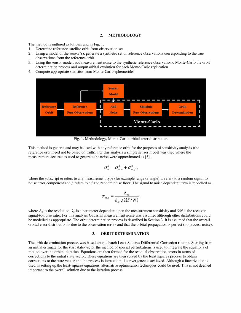
2. METHODOLOGY

The method is outlined as follows and in Fig. 1:

1. Determine reference satellite orbit from observation set

2. Using a model of the sensor(s), generate a synthetic set of reference observations corresponding to the true observations from the reference orbit

3. Using the sensor model, add measurement noise to the synthetic reference observations, Monte-Carlo the orbit

determination process and output orbital evolution for each Monte-Carlo replication

4. Compute appropriate statistics from Monte-Carlo ephemerides

Fig. 1. Methodology, Monte-Carlo orbital error distribution

This method is generic and may be used with any reference orbit for the purposes of sensitivity analysis (the reference orbit need not be based on truth). For this analysis a simple sensor model was used where the

measurement accuracies used to generate the noise were approximated as [3],

2

,

2

,

2

fmnmm σσσ += ,

where the subscript m refers to any measurement type (for example range or angle), n refers to a random signal to

noise error component and f refers to a fixed random noise floor. The signal to noise dependent term is modelled as,

( )NSkm

m

nm/2

,

∆=σ ,

where ∆m is the resolution, km is a parameter dependent upon the measurement sensitivity and S/N is the receiver

signal-to-noise ratio. For this analysis Gaussian measurement noise was assumed although other distributions could

be modelled as appropriate. The orbit determination process is described in Section 3. It is assumed that the overall

orbital error distribution is due to the observation errors and that the orbital propagation is perfect (no process noise).

3. ORBIT DETERMINATION

The orbit determination process was based upon a batch Least Squares Differential Correction routine. Starting from

an initial estimate for the start state-vector the method of special perturbations is used to integrate the equations of

motion over the orbital duration. Equations are then formed for the residual observation errors in terms of corrections to the initial state vector. These equations are then solved by the least squares process to obtain

corrections to the state vector and the process is iterated until convergence is achieved. Although a linearization is

used in setting up the least-squares equations, alternative optimisation techniques could be used. This is not deemed

important to the overall solution due to the iteration process.

The orbital numerical integration used was an adaptive step-size Bulirsch-Stoer routine using a fixed output step [4].

The force model included a 20 by 20 gravity field using the gravity field model EGM96 [5]. Direct luni-solar

perturbations were also modelled [6] and a mean along-track drag deceleration was determined as an unknown state

parameter. To form the least squares equations the state transition matrix between the start state vector and the state

at any given observation time is also required. This is obtained by numerically integrating these partial derivatives

and is performed together with the state vector itself when integrating the equations of motion.

4. ANALYSIS

The METOP Low Earth Orbit (LEO) satellite was chosen for this analysis for which four descending (north-south)

orbital passes of the UK Science and Technology Facilities Council (STFC) Chilbolton radar were available over a

five day period. This is a meteorological radar which has been modified for use for the purposes of demonstration

and testing for space surveillance [7]. Range only measurements were used since this radar does not currently have a

monopulse angle tracking facility. The radar pointing was performed on the basis of predicted Two-Line Elements

(TLEs). The residual Root-Mean Square (RMS) observation error achieved for all passes was less than 100 metres.

The start state vector obtained for this orbit was used to generate the reference orbit.

Fig. 2. The STFC Chilbolton radar facility

The method of analysis outlined in Section 2 was used to estimate the evolution of the orbital error distribution.

However, the purpose of this analysis is to outline the technique used and the methodology, rather than to

demonstrate the utility of this particular radar. As such the sensor model was not chosen to exactly match the actual

observation process, and the results presented here are illustrative only.

In the following analysis the effects of different sensor scenarios on the orbital error evolution is investigated. These

include:

• Number and type (ascending or descending) of satellite pass

• Inclusion of a second sensor in southern hemisphere

• Effect of un-calibrated sensor bias errors.

The geometry and radar coverage is illustrated in Fig. 3 (a) for the UK Chilbolton radar and Fig 3 (b) for the

fictitious second sensor located in Australia. The analysis incorporated various combinations of the orbital passes for

the sensor geometry within the five day orbital period. For this work the period of the analysis was limited to within

the orbital period since the focus here was to investigate the within-orbit errors. However, the method is also ideally

suited for investigating forward predicted orbital errors and the nature of the statistical distribution, as performed in

[2].

Fig. 3. (a) – top, UK Chilbolton radar coverage (green) and METOP orbital geometry (red); and (b) - bottom,

fictitious Australian “Chilbolton” radar coverage (green) and METOP orbital geometry (red).

5. RESULTS

5.1 Effect of pass geometry

Fig. 4 shows the evolution of the orbital position uncertainty (RMS) over the five day duration as obtained from the

Monte-Carlo statistics. The results are for three different satellite pass geometry scenarios for the single sensor

located at the Chilbolton radar site. The geometries are:

a. Four descending (north to south) orbit passes (blue)

b. Two ascending (south to north) and two descending (north to south) orbit passes (green) c. Four ascending (south to north) and four descending (north to south) orbit passes (red)

For clarity Fig. 5 shows the same results but over a reduced duration (1-day). The figures show clearly the effect of

the number of passes and the geometry together with the once per orbital revolution short-periodic variation in the

orbital accuracy. For scenario (a) with four descending passes the overall accuracy varies between approximately 20

metres in the northern hemisphere and 250 metres in the southern. For scenario (b) where two descending passes are

replaced by two adjacent ascending passes there is clearly a generally smaller range in the achieved accuracy. If four

ascending and four descending passes are utilised as in (c) the overall orbital accuracy is significantly increased

(variation between approximately 13–29 metres). It can be seen from the figures that, when the satellite is in the

northern hemisphere (corresponding to sensor latitude), the best accuracy is achieved, whilst the accuracy is severely

diminished at corresponding times when the satellite is in the southern hemisphere.

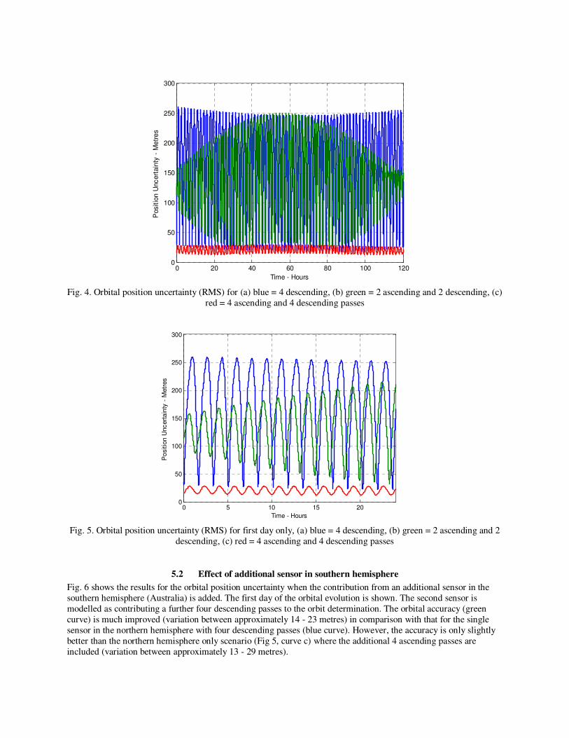
Fig. 4. Orbital position uncertainty (RMS) for (a) blue = 4 descending, (b) green = 2 ascending and 2 descending, (c)

red = 4 ascending and 4 descending passes

Fig. 5. Orbital position uncertainty (RMS) for first day only, (a) blue = 4 descending, (b) green = 2 ascending and 2

descending, (c) red = 4 ascending and 4 descending passes

5.2 Effect of additional sensor in southern hemisphere

Fig. 6 shows the results for the orbital position uncertainty when the contribution from an additional sensor in the

southern hemisphere (Australia) is added. The first day of the orbital evolution is shown. The second sensor is

modelled as contributing a further four descending passes to the orbit determination. The orbital accuracy (green

curve) is much improved (variation between approximately 14 - 23 metres) in comparison with that for the single

sensor in the northern hemisphere with four descending passes (blue curve). However, the accuracy is only slightly

better than the northern hemisphere only scenario (Fig 5, curve c) where the additional 4 ascending passes are

included (variation between approximately 13 - 29 metres).

0 20 40 60 80 100 1200

50

100

150

200

250

300

Time - Hours

Posit

ion

Unc

ert

ain

ty -

Me

tre

s

0 5 10 15 200

50

100

150

200

250

300

Time - Hours

Po

sitio

n U

nc

ert

ain

ty -

Metr

es

Fig. 6. - Orbital position uncertainty (RMS) for first day, (a) blue = 4 descending using only northern hemisphere

sensor (as per Fig 5a), (b) green = 4 descending + 4 descending passes from 2nd sensor in southern hemisphere

5.3 Effect of residual sensor bias

Fig. 7 shows the effect of a 100 metre uncompensated residual sensor bias error (single sensor scenario), again for

the first day of the orbital evolution. This has been modelled as a Gaussian random variable which varies from pass

to pass but is fixed for each individual pass. The orbital error and its variation with latitude are now substantially

increased and now vary between approximately 250 metres and 3100 metres.

Fig. 7. Orbital position uncertainty (RMS) for first day (a) blue = 4 descending (as per Fig 5a) , (b) green = 4

descending with 100 metre residual sensor bias error (single sensor scenario)

6. SENSOR NETWORK CONSIDERATIONS

0 5 10 15 200

50

100

150

200

250

300

Time - Hours

Po

sitio

n U

ncert

ain

ty -

Metr

es

0 5 10 15 200

500

1000

1500

2000

2500

3000

3500

Time - Hours

Po

sitio

n U

ncert

ain

ty -

Metr

es

Surveillance of space presents an enormous challenge due to the small size of some of the objects that need to be

tracked and the huge volume to be searched. The total volume of space out to GEO orbits is of the order of 1023 m3.

A typical orbital path is 107 m but increasingly we may be required to know the position of an object to within a few

meters. Individual sensors have limited accuracy and as shown in the preceding analysis, there is an uncertainty in

the sensor measurement and the uncertainty in an object’s position grows once it is out of sensor coverage. Hence

the nature of space situational awareness (providing a complete and accurate picture of space objects) means that globally distributed sensor networks are needed to give comprehensive and consistent metric information about the

objects of interest. Clearly effective ways of fitting observations to orbits and appropriate orbital propagation

methods are needed. However the wider context also needs to be considered for evaluation of whole systems issues

and solutions.

In considering a space surveillance network there are a number of constraints that will apply. These will dictate the

degree of sophistication, the robustness of orbital determination and propagation methods (with associated

processing requirements) and the capability of individual sensors needed to meet particular requirements. In broad

terms these constraints may include; location, availability, coverage, orientation, sensor characteristics and

capability, and the ability to fuse data of different characteristics from different sensors. The sensor characteristics

have trade-offs to be considered in evaluation of individual sensors such as measurement accuracy, update rate,

number of objects that can be catered for contemporaneously, and type of observation that can be made. For optical systems this will typically include angle and signature fluctuations, and for active radar the observations will be

range, angle, as well as possibly Doppler and signature fluctuations.

Sensors can be land based, ship based or even air or space based. Some sensors may also be deployable or movable.

Estimation of sensor capability and methods of fusion, taking into account these characteristics and trade-offs, are

necessary to evolve an ability for effective network design and evaluation. Given the large number of variables

within this problem space an efficient method to assess the potential solutions is required. This is discussed further

in Section 7.

7. PERFORMANCE PREDICTION FOR A SENSOR NETWORK One of the tools available to explore the effect of geographical location and the type of sensor observation is the

Cramér-Rao Lower Bound (CRLB) [8]. The CRLB is a theoretical construction which, given an object trajectory

and sensor models, allows analytical determination of a lower bound on the average position error that is

independent of the type of estimator (assuming that the estimator is unbiased). Thus the bound gives a prediction of

the on-average system performance without explicitly performing estimation. These predictions can be evaluated at

a very low computational cost, permitting the exploration of networks with a variety of sensor types and locations.

The Tracking and Sensor Fusion (TSF) group at DSTO is a centre for expertise in low-level data fusion, especially

in the creation, association and fusion of tracks. The team has substantial practical expertise in multi-sensor, multi-

target tracking and various aspects of multi-sensor fusion, including fusion architectures and bias compensation.

TSF group is currently acquiring and developing a network of optical sensors, primarily using commercial off-the-

shelf equipment, for evaluation of new tracking and fusion algorithms applied to surveillance of space. Potential contributions of this system to SoSp will be gauged in collaboration with Dstl, leveraging some of the existing and

emerging SoSp assets in the UK and Australia. One of the benchmarks that are used to assess and compare the

quality of these algorithms is the Cramér-Rao lower bound.

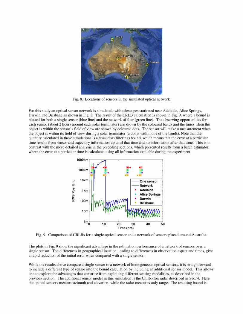
Fig. 8. Locations of sensors in the simulated optical network.

For this study an optical sensor network is simulated, with telescopes stationed near Adelaide, Alice Springs, Darwin and Brisbane as shown in Fig. 8. The result of the CRLB calculation is shown in Fig. 9, where a bound is

plotted for both a single sensor (blue line) and the network of four (green line). The observing opportunities for

each sensor (about 2 hours around each solar terminator) are shown by the coloured bands and the times when the

object is within the sensor’s field of view are shown by coloured dots. The sensor will make a measurement when

the object is within its field of view during a solar terminator (a dot is within one of the bands). Note that the

quantity calculated in these simulations is a posterior (filtering) bound, which means that the error at a particular

time results from sensor and trajectory information up until that time and no information after that time. This is in

contrast with the more detailed analysis in the preceding sections, which presented results from a batch estimator,

where the error at a particular time is calculated using all information available during the experiment.

Fig. 9. Comparison of CRLBs for a single optical sensor and a network of sensors placed around Australia.

The plots in Fig. 9 show the significant advantage in the estimation performance of a network of sensors over a

single sensor. The differences in geographical location, leading to differences in observation aspect and times, give

a rapid reduction of the initial error when compared with a single sensor.

While the results above compare a single sensor to a network of homogeneous optical sensors, it is straightforward

to include a different type of sensor into the bound calculation by including an additional sensor model. This allows

one to explore the advantages that can arise from exploiting different sensing modalities, as described in the

previous section. The additional sensor model in this simulation is the Chilbolton radar described in Sec. 4. Here the optical sensors measure azimuth and elevation, while the radar measures only range. The resulting bound is

0 10 20 30 40 501m

10m

100m

1km

10km

100km

1000km

RM

S P

os. E

rr.

Time (hrs)

One sensor

Network

Adelaide

Alice Springs

Darwin

Brisbane

shown in Fig. 10, comparing the bound obtained from the network of optical sensors with the bound obtained from

the network and the radar. In Fig. 10 the dots show the times when the object is observable by each sensor. Once

again the geographic diversity leads to a substantial improvement in the estimation accuracy that can be theoretically

obtained. In this case there is an additional benefit in that the radar measures the location of the object in a different

way to the optical sensors.

Fig. 10. Comparison of CRLBs for a network of heterogeneous sensors (optical and radar; green) as compared to a

network of homogenous sensors (optical; blue).

The results presented in Fig. 9 and Fig. 10 should be considered as best case as they are computed with idealised

trajectories and sensor models. Firstly they are calculated assuming that the object trajectory is deterministic, that is

there is no allowance for unknown or un-modelled forces in the propagation model. Secondly these bounds are

calculated without modeling persistent sensor bias, calibration inaccuracies or timing inaccuracies. Similarly it is

assumed that the object is within the sensor’s field-of view where feasible, neglecting issues of tasking, object

association and limited a-priori ephemeris information. However the bound does provide a very good indication of

the relative errors between two sensor systems and this type of calculation has been widely used for performance

prediction in the tracking literature with considerable success [9].

8. DISCUSSION (SENSOR NETWORKS) The techniques discussed in the previous section show the complexity and variation of the orbital error for possible

configurations of sensor networks. It illustrates that having multiple sensors is beneficial in all cases investigated

and that the errors have short term variations with an increasingly degrading drift which can be reduced when the

opportunity for observation from one or more different sites occurs.

Such techniques can therefore be used to evaluate the utility of particular sensors and sensor mixes. However a key

point that emerges is that it is also necessary to establish definitive requirements both in terms of accuracy and the

time scales needed to achieve this accuracy. This applies to both newly detected and re-located ‘lost’ objects. In

determining optimal sensor networks or the benefits of new or improved sensors, their characteristics must also be

considered. In general optical systems will be subject to illumination conditions and weather restrictions which do

not affect radar. On the other hand, radar performance reduces by the 4th power of range whereas optical performance is determined by an inverse-square law. This leads to the preferential use of certain sensor types for

certain orbital regimes and there are many other constraints and wider issues that need to be considered. More

details of these and the relevant trade-offs can be found in [10]. Using the CRLB, together with gaining a better

understanding of the influence of effects such as sensor bias and having a definitive set of requirements, we are

starting to evolve better methods of evaluating and comparing different sensor and network solutions.

0 10 20 30 40 501m

10m

100m

1km

10km

RM

S P

os

. E

rr.

Time (hrs)

Optical

Optical + Radar

Optical

Chilbolton

9. CONCLUSIONS

This paper uses a Monte-Carlo technique to analyse the evolution of the orbital error of a space object due to

observational uncertainties. Some examples of how the method may be used to analyse the effects of sensor and pass

geometry on the error evolution have been given considering a single LEO satellite. However, the analysis and

method can easily be extended to investigate effects such as extent of non-linearity for a given scenario; extent of non-Gaussian behavior for a given scenario and the effect of different sensor models and statistics. A CRLB analysis

demonstrates the performance benefits that can be achieved for a sensor network over that for a single sensor, and

when fusing data from various sensor types. Establishing definitive requirements for accuracy and the time to

achieve it is also a key enabler for evaluating the benefit of particular sensors and sensor network performance.

10. ACKNOWLEDGEMENT

The authors would like to thank Jon Eastment, STFC, UK for making available measurements from the Chilbolton

Observatory radar facility.

11. REFERENCES 1. Vallado, D. A. Fundamentals of Astrodynamics and Applications, Third Edition, Microcosm Press, Springer,

2007.

2. Sabol C. S., Sukut S., Hill K., Alfriend K. T., Wright, B, Li Y., Schumacher P., Linearized Orbit Covariance

Generation and Propagation Analysis via Simple Monte Carlo Simulations, American Astronautical Society,

Advances in the Astronautics Sciences, Volume 136, 2010.

3. Curry G. R. Radar System Performance Modelling, 2nd Edition, Artech House, 2005.

4. Press W. H, Teukolsky S. A, Vetterling W. T.. and Flannery B. P., Numerical Recipes, Third Edition,

Cambridge University Press, 2007.

5. Lemoine F. G., Kenyon S. C., Factor J. K., Trimmer R. G., Pavlis N. K., Chinn D. S., Cox C. M., Klosko S. M.,

Luthcke S. B., Torrence M. H., Wang Y. M., Williamson R. G., Pavlis E. C., Rapp R. H., Olson T. R., The

Development of the Joint NASA GSFC and NIMA Geopotential Model EGM96; NASA/GSFC, NASA/TP-1998-206891, 1998.

6. Montenbruck O. and Gill, E., Satellite Orbits, Springer, 2000.

7. Eastment J. D., Ladd, D. N., Walden C. J. and Trethewey M. L., Satellite Observations using the Chilbolton

Radar during the Initial ESA ‘CO-V1’ Tracking Campaign. To be published in Proceedings of European Space

Surveillance Conference, Marid, Spain, 2011

8. Taylor J. H., The Cramér-Rao Estimation Error Lower Bound Computation for Deterministic Nonlinear

Systems, IEEE Transactions on Automatic Control, pp. 343-344, Vol. 24, No. 2, Apr. 1979.

9. Ristic B., Arulampalam S. and Gordon N. J., Beyond the Kalman Filter: Particle Filters for Tracking

Applications, Artech House, 2004.

10. Donnelly R.P, Condley C, Surveillance of Space – Optimal Use of Complementary Sensors for Maximum

Efficiency, NATO RTO SET 105 Specialists Meeting, 2006.