1 1 Slide Chapter 11, Part B Chapter 11, Part B Inventory Models: Probabilistic Demand Inventory Models: Probabilistic Demand Lecture Outline Lecture Outline • Single Single- - Period Inventory Model with Probabilistic Demand Period Inventory Model with Probabilistic Demand • Order Order- -Quantity, Reorder Quantity, Reorder- - Point Model with Probabilistic Point Model with Probabilistic Demand Demand • Periodic Periodic- - Review Model with Probabilistic Demand Review Model with Probabilistic Demand 2 Slide

Welcome message from author
This document is posted to help you gain knowledge. Please leave a comment to let me know what you think about it! Share it to your friends and learn new things together.
Transcript
8/2/2019 Or B Inventory Models
http://slidepdf.com/reader/full/or-b-inventory-models 1/25
1
1Slide
Chapter 11, Part BChapter 11, Part B
Inventory Models: Probabilistic DemandInventory Models: Probabilistic Demand
Lecture OutlineLecture Outline
•• SingleSingle--Period Inventory Model with Probabilistic DemandPeriod Inventory Model with Probabilistic Demand
•• OrderOrder--Quantity, ReorderQuantity, Reorder--Point Model with ProbabilisticPoint Model with ProbabilisticDemandDemand
•• PeriodicPeriodic--Review Model with Probabilistic DemandReview Model with Probabilistic Demand
2Slide
8/2/2019 Or B Inventory Models
http://slidepdf.com/reader/full/or-b-inventory-models 2/25
2
3Slide
Probabilistic ModelsProbabilistic Models
In many cases demand (or some other factor) is notIn many cases demand (or some other factor) is notknown with a high degree of certainty and aknown with a high degree of certainty and aprobabilistic inventory modelprobabilistic inventory model should actually beshould actually beused.used.
These models tend to be more complex thanThese models tend to be more complex thandeterministic models.deterministic models.
The probabilistic models covered in this chapter are:The probabilistic models covered in this chapter are:
•• singlesingle--period order quantityperiod order quantity
•• reorderreorder--point quantitypoint quantity
•• periodicperiodic--review order quantityreview order quantity
4Slide
8/2/2019 Or B Inventory Models
http://slidepdf.com/reader/full/or-b-inventory-models 3/25
3
5Slide
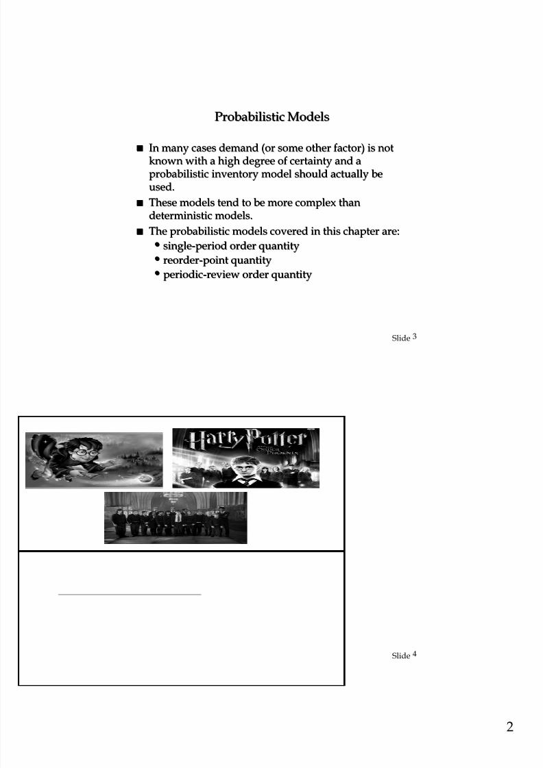
Harry Potter and the Order of the Phoenix by JKHarry Potter and the Order of the Phoenix by JKRowling 5thRowling 5th
This book sold over a millionThis book sold over a millioncopies in 1 day throughcopies in 1 day throughAmazon alone.Amazon alone.
Ten million copies were soldTen million copies were soldin the first 3 days (Englishin the first 3 days (Englishversion alone).version alone).
long queues of millionslong queues of millionswaiting for the opening ofwaiting for the opening ofbookstores.bookstores.
If they canIf they can’’t buy it first weekt buy it first weekthey donthey don’’t want to buy it .t want to buy it .
The publishers were underThe publishers were underpressure to produce thepressure to produce therequired amount of booksrequired amount of books
6Slide
Newsboy problem: SingleNewsboy problem: Single--Period Order QuantityPeriod Order Quantity
AA singlesingle--period order quantity modelperiod order quantity model (sometimes(sometimescalled the newsboy problem) deals with a situation incalled the newsboy problem) deals with a situation inwhich onlywhich only one order is placedone order is placed for the item and thefor the item and thedemand is probabilisticdemand is probabilistic..
D > Q If the period's demand exceeds the orderD > Q If the period's demand exceeds the order
quantity, the demand is not backordered andquantity, the demand is not backordered andrevenue (profit)revenue (profit) will be lostwill be lost..
D < Q If demand is less than the order quantity, theD < Q If demand is less than the order quantity, thesurplus stocksurplus stock is sold at the end of the period (usuallyis sold at the end of the period (usuallyfor less than the original purchase price).for less than the original purchase price).
8/2/2019 Or B Inventory Models
http://slidepdf.com/reader/full/or-b-inventory-models 4/25
4
7Slide
SingleSingle--Period Order QuantityPeriod Order Quantity
When To use SingleWhen To use Single--period inventory model withperiod inventory model withProbabilistic Demand.Probabilistic Demand.
•• Seasonal or perishable items.Seasonal or perishable items.
•• CanCan’’t be carried in the inventory.t be carried in the inventory.
•• CanCan’’t be sold in the futuret be sold in the future
Ex:Ex:
•• News PapersNews Papers
•• FashionsFashions
•• Computer booksComputer books
•• GadgetsGadgets
•• Harry Potter BooksHarry Potter Books
8Slide
SingleSingle--Period Order QuantityPeriod Order Quantity
One question only is in placeOne question only is in place
•• How much of the products should we orderHow much of the products should we order
•• There is no question such as when we shouldThere is no question such as when we shouldreorder.reorder.
8/2/2019 Or B Inventory Models
http://slidepdf.com/reader/full/or-b-inventory-models 5/25
5
9Slide
SingleSingle--Period Order QuantityPeriod Order Quantity
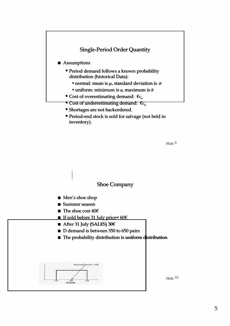
AssumptionsAssumptions
•• Period demand follows a known probabilityPeriod demand follows a known probabilitydistribution (historical Data):distribution (historical Data):
•• normal: mean isnormal: mean is µ µ , standard deviation is, standard deviation is σ σ
•• uniform: minimum isuniform: minimum is aa, maximum is, maximum is bb
•• Cost of overestimating demand:Cost of overestimating demand: € €ccoo
•• Cost of underestimating demand:Cost of underestimating demand: € €ccuu
•• Shortages are not backordered.Shortages are not backordered.
•• PeriodPeriod--end stock is sold for salvage (not held inend stock is sold for salvage (not held ininventory).inventory).
10Slide
Shoe CompanyShoe Company
MenMen’’s shoe shops shoe shop
Summer seasonSummer season
The shoe cost 40The shoe cost 40 € €
If sold before 31 July price= 60If sold before 31 July price= 60 € €
After 31 July (SALES) 30After 31 July (SALES) 30 € €
D demand is between 350 to 650 pairsD demand is between 350 to 650 pairs
The probability distribution is uniform distributionThe probability distribution is uniform distribution

8/2/2019 Or B Inventory Models
http://slidepdf.com/reader/full/or-b-inventory-models 6/25
6
11Slide
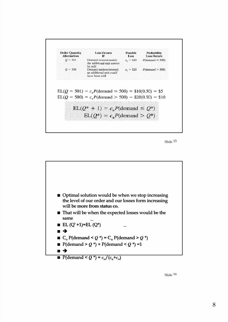
CCoo =30=30--40=1040=10 € €..
Loss because we sell inLoss because we sell incheaper pricecheaper price
CCuu=60=60--40=2040=20 € €..
Loss because we lose theLoss because we lose theopportunity to winopportunity to win
The big question is if we assume are selling 500The big question is if we assume are selling 500
Is it worth to sell 501, what are our expected lossesIs it worth to sell 501, what are our expected losses
12Slide
What are our losses, in the following optionsWhat are our losses, in the following options
Increase our order quantity by 1Increase our order quantity by 1
Q=501Q=501
Our losses will be in ourOur losses will be in ourinability to sell the additionalinability to sell the additionalunit ( we over estimated ourunit ( we over estimated ourdemand) we sell it in cheaperdemand) we sell it in cheaper
priceprice CCoo =10=10 € €..
P(D<501)=P(DP(D<501)=P(D<<500)=150/300500)=150/300
EL(Q=501) =EL(Q=501) =
P* CP* Coo = .5 *10== .5 *10= 55
Stay at 500 orderStay at 500 order
Q=500Q=500
Our Losses will be in ourOur Losses will be in ourinability to fulfil our demandinability to fulfil our demandlosing the opportunity to win.losing the opportunity to win.
CCuu=20=20 € €
P(D>500)=150/300P(D>500)=150/300
EL( Q=500) =EL( Q=500) =
P* CP* Cuu = .5 *20== .5 *20= 1010

8/2/2019 Or B Inventory Models
http://slidepdf.com/reader/full/or-b-inventory-models 7/25
7
13Slide
What are our losses, in the following optionsWhat are our losses, in the following options
Increase our order quantity by 1Increase our order quantity by 1
Q=502Q=502
Our losses will be in ourOur losses will be in ourinability to sell the additionalinability to sell the additionalunit ( we over estimated ourunit ( we over estimated ourdemand) we sell it in cheaperdemand) we sell it in cheaperpriceprice
CCoo =10=10 € €..
P(D<502)=P(DP(D<502)=P(D<<501)=151/300501)=151/300
EL(Q=501) =EL(Q=501) =
P* CP* Coo = .5033 *10== .5033 *10= 5.0335.033
Stay at 501 orderStay at 501 order
Q=501Q=501
Our Losses will be in ourOur Losses will be in ourinability to fulfil our demandinability to fulfil our demandlosing the opportunity to win.losing the opportunity to win.
CCuu=20=20 € €
P(D>501)=149/300P(D>501)=149/300
EL( Q=500) =EL( Q=500) =
P* CP* Cuu = .4966 *20== .4966 *20= 9,9339,933
14Slide
What are our losses, in the following optionsWhat are our losses, in the following options
Increase our order quantity by 1Increase our order quantity by 1
Q=601Q=601
Our losses will be in ourOur losses will be in ourinability to sell the additionalinability to sell the additionalunit ( we over estimated ourunit ( we over estimated ourdemand) we sell it in cheaperdemand) we sell it in cheaper
priceprice CCoo =10=10 € €..
P(D<601)=P(DP(D<601)=P(D<<600)=250/300600)=250/300
EL(Q=501) =EL(Q=501) =
P* CP* Coo = .8333 *10== .8333 *10= 8,338,33
Stay at 500 orderStay at 500 order
Q=600Q=600
Our Losses will be in ourOur Losses will be in ourinability to fulfil our demandinability to fulfil our demandlosing the opportunity to win.losing the opportunity to win.
CCuu=20=20 € €
P(D>600)=50/300P(D>600)=50/300
EL( Q=500) =EL( Q=500) =
P* CP* Cuu = .1667 *20== .1667 *20= 3.333.33
8/2/2019 Or B Inventory Models
http://slidepdf.com/reader/full/or-b-inventory-models 8/25
8
15Slide
16Slide
Optimal solution would be when we stop increasingOptimal solution would be when we stop increasingthe level of our order and our losses form increasingthe level of our order and our losses form increasingwill be more from status co.will be more from status co.
That will be when the expected losses would be theThat will be when the expected losses would be thesamesame
EL (QEL (Q**
+1)=EL (Q*)+1)=EL (Q*)
CCoo P(demandP(demand << QQ *) = C*) = Cuu P(demandP(demand >> QQ *)*)
P(demandP(demand >> QQ *) +*) + P(demandP(demand << QQ *) =1*) =1
P(demandP(demand << QQ *) =*) = ccuu/(/(ccuu++ccoo))
8/2/2019 Or B Inventory Models
http://slidepdf.com/reader/full/or-b-inventory-models 9/25
9
17Slide
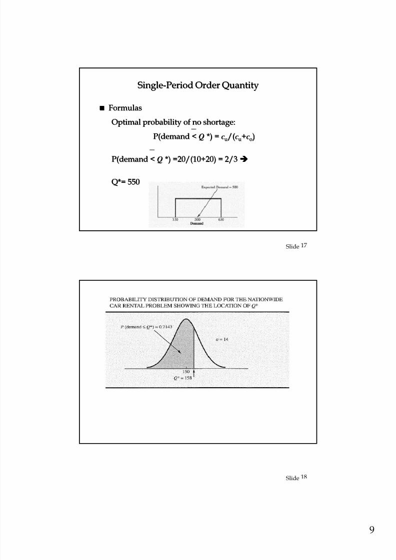
FormulasFormulas
Optimal probability of no shortage:Optimal probability of no shortage:
P(demandP(demand << QQ *) =*) = ccuu/(/(ccuu++ccoo))
P(demandP(demand << QQ *) =20/(10+20) = 2/3*) =20/(10+20) = 2/3
Q*= 550Q*= 550
SingleSingle--Period Order QuantityPeriod Order Quantity
18Slide
8/2/2019 Or B Inventory Models
http://slidepdf.com/reader/full/or-b-inventory-models 10/25
10
19Slide
FormulasFormulas
Optimal probability of no shortage:Optimal probability of no shortage:
P(demandP(demand << QQ *) =*) = ccuu/(/(ccuu++ccoo))
Optimal order quantity, based on demand distribution:Optimal order quantity, based on demand distribution:
normal:normal: QQ * =* = µ µ ++ z zσ σ
uniform:uniform: QQ * =* = aa + P(demand+ P(demand << QQ *)(*)(bb--aa))
SingleSingle--Period Order QuantityPeriod Order Quantity
20Slide
Example:Example: McHardeeMcHardee PressPress
SingleSingle--Period Order QuantityPeriod Order Quantity
•• McHardeeMcHardee Press publishes the FastPress publishes the FastFood Menu Book and wishes toFood Menu Book and wishes todetermine how many copies todetermine how many copies toprint.print.
•• the incremental profit per copy isthe incremental profit per copy is$0.45.$0.45.
•• Any unsold copies of the book canAny unsold copies of the book canbe sold at salvage at a $.55 loss.be sold at salvage at a $.55 loss.
8/2/2019 Or B Inventory Models
http://slidepdf.com/reader/full/or-b-inventory-models 11/25
11
21Slide
Example:Example: McHardeeMcHardee PressPress
SingleSingle--Period Order QuantityPeriod Order Quantity
Sales for this edition are estimated to be normallySales for this edition are estimated to be normallydistributed. The most likely sales volume is 12,000distributed. The most likely sales volume is 12,000copies , with standard deviationcopies , with standard deviation 4848.4848.
How many copies should be printed?How many copies should be printed?
22Slide
Example:Example: McHardeeMcHardee PressPress
SingleSingle--Period Order QuantityPeriod Order Quantity
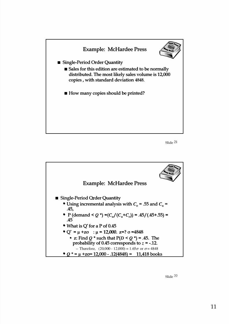
•• Using incremental analysis withUsing incremental analysis with C C oo = .55 and= .55 and C C uu ==.45,.45,
•• P (demandP (demand << QQ *) =(*) =(C C uu/(/(C C uu++C C oo)) = .45/(.45+.55) =)) = .45/(.45+.55) =.45.45
•• What is QWhat is Q**
for a P of 0.45for a P of 0.45•• QQ** == µµ +z+zσσ :: µµ = 12,000. z=?= 12,000. z=? σσ ==48484848
•• z: Findz: Find QQ * such that P(* such that P( D D << QQ *) = .45. The*) = .45. Theprobability of 0.45 corresponds toprobability of 0.45 corresponds to z z == --.12..12.
– Therefore, (20,000 - 12,000) = 1.65σ or σ = 4848
•• QQ * =* = µµ +z+zσσ== 12,00012,000 -- .12(4848) = 11,418 books.12(4848) = 11,418 books
8/2/2019 Or B Inventory Models
http://slidepdf.com/reader/full/or-b-inventory-models 12/25
12
23Slide
Example:Example: McHardeeMcHardee PressPress
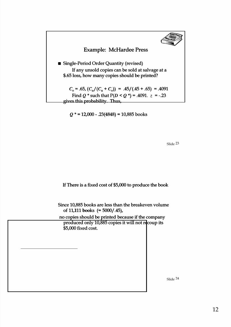
SingleSingle--Period Order Quantity (revised)Period Order Quantity (revised)
If any unsold copies can be sold at salvage at aIf any unsold copies can be sold at salvage at a$.65 loss, how many copies should be printed?$.65 loss, how many copies should be printed?
C C oo = .65, (= .65, (C C uu/(/(C C uu ++ C C oo)) = .45/(.45 + .65) = .4091)) = .45/(.45 + .65) = .4091
FindFind QQ * such that P(* such that P( D D << QQ *) = .4091.*) = .4091. z z == --.23.23gives this probability. Thus,gives this probability. Thus,
QQ * = 12,000* = 12,000 -- .23(4848) = 10,885 books.23(4848) = 10,885 books
24Slide
If There is a fixed cost of $5,000 to produce the bookIf There is a fixed cost of $5,000 to produce the book
Since 10,885 books are less than the breakeven volumeSince 10,885 books are less than the breakeven volumeof 11,111 books (= 5000/.45),of 11,111 books (= 5000/.45),
no copies should be printedno copies should be printed because if the companybecause if the companyproduced only 10,885 copies it will not recoup itsproduced only 10,885 copies it will not recoup its
$5,000 fixed cost.$5,000 fixed cost.
8/2/2019 Or B Inventory Models
http://slidepdf.com/reader/full/or-b-inventory-models 13/25
13
25Slide
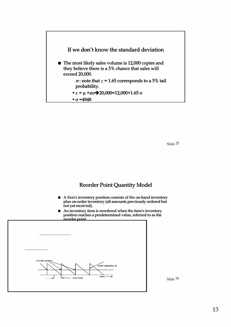
If we donIf we don’’t know the standard deviationt know the standard deviation
The most likely sales volume is 12,000 copies andThe most likely sales volume is 12,000 copies andthey believe there is a 5% chance that sales willthey believe there is a 5% chance that sales willexceed 20,000.exceed 20,000.
σ σ : note that: note that z z = 1.65 corresponds to a 5% tail= 1.65 corresponds to a 5% tailprobability.probability.
•• x x == µµ +z+zσσ20,000=12,000+1.6520,000=12,000+1.65 σσ
•• σσ ==48484848
26Slide
Reorder Point Quantity ModelReorder Point Quantity Model
A firm'sA firm's inventory positioninventory position consists of the onconsists of the on--hand inventoryhand inventoryplus onplus on--order inventory (all amounts previously ordered butorder inventory (all amounts previously ordered butnot yet received).not yet received).
An inventory item is reordered when the item's inventoryAn inventory item is reordered when the item's inventoryposition reaches a predetermined value, referred to as theposition reaches a predetermined value, referred to as thereorder pointreorder point..

8/2/2019 Or B Inventory Models
http://slidepdf.com/reader/full/or-b-inventory-models 14/25
14
27Slide
The reorder point represents the quantity available toThe reorder point represents the quantity available tomeet demand during lead timemeet demand during lead time..
Lead timeLead time is the time span starting when theis the time span starting when thereplenishment order is placed and ending when thereplenishment order is placed and ending when theorder arrives.order arrives.
28Slide
Reorder Point QuantityReorder Point Quantity
Under deterministic conditions, when both demandUnder deterministic conditions, when both demandand lead time are constant, theand lead time are constant, the reorder pointreorder pointassociated with EOQassociated with EOQ--based modelsbased models is set equalis set equal totolead time demand.lead time demand.
Under probabilistic conditions, when demandUnder probabilistic conditions, when demand
and/or lead time varies, the reorder point oftenand/or lead time varies, the reorder point oftenincludesincludes safety stock.safety stock.
Safety stockSafety stock is the amount by which the reorder pointis the amount by which the reorder pointexceeds the expected (average) lead time demand.exceeds the expected (average) lead time demand.

8/2/2019 Or B Inventory Models
http://slidepdf.com/reader/full/or-b-inventory-models 15/25
15
29Slide
30Slide
Safety Stock and Service LevelSafety Stock and Service Level
The amount of safety stock in a reorder pointThe amount of safety stock in a reorder pointdetermines the chance of adetermines the chance of a stockoutstockout during lead time.during lead time.
The complement of this chance is called theThe complement of this chance is called the serviceservicelevel.level.
Service levelService level, in this context, is defined as the, in this context, is defined as the
probability of not incurring aprobability of not incurring a stockoutstockout during anyduring anyone lead time.one lead time.
Service level, in this context, also is the longService level, in this context, also is the long--runrunproportion of lead times in which noproportion of lead times in which no stockoutsstockouts occur.occur.
8/2/2019 Or B Inventory Models
http://slidepdf.com/reader/full/or-b-inventory-models 16/25
16
31Slide
Reorder Point ModelReorder Point Model
AssumptionsAssumptions
•• LeadLead--time demand is normally distributedtime demand is normally distributed
with meanwith mean µ µ and standard deviationand standard deviation σ σ ..
•• Approximate optimal order quantity: EOQApproximate optimal order quantity: EOQ
•• Service level is defined in terms of the probability ofService level is defined in terms of the probability ofnono stockoutsstockouts during lead time and is reflected induring lead time and is reflected in z z ..
•• Shortages are not backordered.Shortages are not backordered.
•• Inventory position is reviewed continuously.Inventory position is reviewed continuously.
32Slide
Reorder Point ModelReorder Point Model
•• Robert's Drugs is a drug wholesaler supplying 55Robert's Drugs is a drug wholesaler supplying 55independent drug stores.independent drug stores.
•• Roberts wishes to determine anRoberts wishes to determine an optimal inventoryoptimal inventory policy policy forfor Comfort Comfort brand headache remedy.brand headache remedy.
•• Sales ofSales of Comfort Comfort are relatively constantare relatively constant
•• as the past 10 weeks of data (on next slide)as the past 10 weeks of data (on next slide)indicate.indicate.
Example: RobertExample: Robert’’s Drugs Drug
8/2/2019 Or B Inventory Models
http://slidepdf.com/reader/full/or-b-inventory-models 17/25
17
33Slide
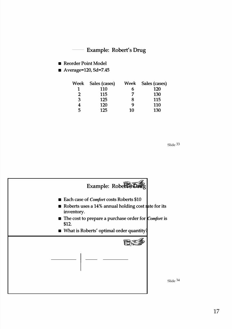
Reorder Point ModelReorder Point Model
Average=120,Average=120, SdSd=7.45=7.45
WeekWeek Sales (cases)Sales (cases) WeekWeek Sales (cases)Sales (cases)11 110110 6 1206 12022 115115 7 1307 13033 125125 8 1158 11544 120120 9 1109 11055 125125 10 13010 130
Example: RobertExample: Robert’’s Drugs Drug
34Slide
Example: RobertExample: Robert’’s Drugs Drug
Each case ofEach case of Comfort Comfort costs Roberts $10costs Roberts $10
Roberts uses a 14% annual holding cost rate for itsRoberts uses a 14% annual holding cost rate for itsinventory.inventory.
The cost to prepare a purchase order forThe cost to prepare a purchase order for Comfort Comfort isis$12.$12.
What is RobertsWhat is Roberts’’ optimal order quantity?optimal order quantity?
8/2/2019 Or B Inventory Models
http://slidepdf.com/reader/full/or-b-inventory-models 18/25
18
35Slide
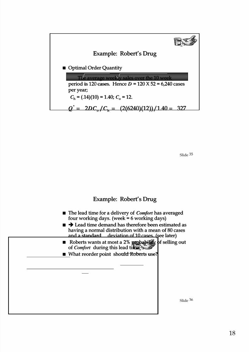
Optimal Order QuantityOptimal Order Quantity
The average weekly sales over the 10 weekThe average weekly sales over the 10 weekperiod is 120 cases. Henceperiod is 120 cases. Hence D D = 120 X 52 = 6,240 cases= 120 X 52 = 6,240 casesper year;per year;
C C hh = (.14)(10) = 1.40;= (.14)(10) = 1.40; C C oo = 12.= 12.
Example: RobertExample: Robert’’s Drugs Drug
*o h2 / (2(6240)(12))/1.40 327Q DC C = = =
*o h2 / (2(6240)(12))/1.40 327Q DC C = = =
36Slide
Example: RobertExample: Robert’’s Drugs Drug
The lead time for a delivery ofThe lead time for a delivery of Comfort Comfort hashas averagedaveragedfour working days.four working days. (week = 6 working days)(week = 6 working days)
Lead time demand has therefore been estimated asLead time demand has therefore been estimated ashaving a normal distribution with a meanhaving a normal distribution with a mean of 80 casesof 80 casesand a standardand a standard deviation of 10 cases.deviation of 10 cases. (see later)(see later)
Roberts wants at most aRoberts wants at most a 2%2% probability of selling outprobability of selling out
ofof Comfort Comfort during this lead time.during this lead time. What reorder point should Roberts use?What reorder point should Roberts use?

8/2/2019 Or B Inventory Models
http://slidepdf.com/reader/full/or-b-inventory-models 19/25
19
37Slide
Example: RobertExample: Robert’’s Drugs Drug
Optimal Reorder PointOptimal Reorder Point
•• Hence Roberts should reorderHence Roberts should reorder Comfort Comfort when supply reacheswhen supply reaches
•• r r == μ μ ++ z zσ σ
•• Lead time demand is normally distributed withLead time demand is normally distributed with μ= μ= mm ==80,80, σ σ = 10 cases= 10 cases
•• Z: Since Roberts wants at most a 2% probability of sellingZ: Since Roberts wants at most a 2% probability of sellingout ofout of Comfort Comfort , the corresponding, the corresponding z z value is 2.06. That is,value is 2.06. That is,PP (( z z > 2.06) = .0197 (about .02).> 2.06) = .0197 (about .02).
•• Hence Roberts should reorderHence Roberts should reorder Comfort Comfort when supply reacheswhen supply reachesr r == μ μ ++ z zσ σ = 80 + 2.06(10) = 101 cases.= 80 + 2.06(10) = 101 cases.
•• The safety stock isThe safety stock is z zσ σ = 21 cases.= 21 cases.
38Slide
8/2/2019 Or B Inventory Models
http://slidepdf.com/reader/full/or-b-inventory-models 20/25
20
39Slide
FormulasFormulas
Reorder point:Reorder point: r r == µ µ ++ z zσ σ
Safety stock:Safety stock: z zσ σ
Average inventory:Average inventory: ½½ ((QQ ) +) + z zσ σ
Total annual cost: [(Total annual cost: [( ½½ ))QQ **C C hh]] ++ [[ z zσ σ C C hh]] ++ [[ DC DC oo//QQ *]*]
(hold.(normal) + hold.(safety)(hold.(normal) + hold.(safety)
+ ordering)+ ordering)
Reorder PointReorder Point
40Slide
Example: RobertExample: Robert’’s Drugs Drug
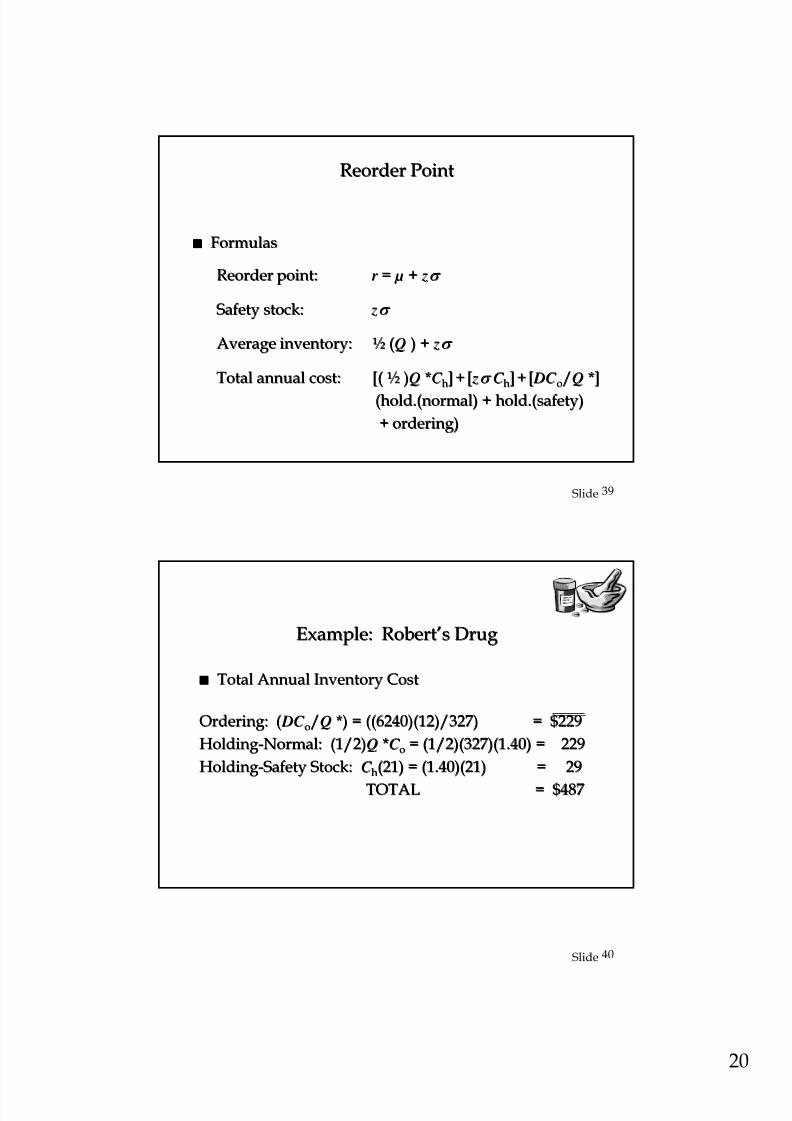
Total Annual Inventory CostTotal Annual Inventory Cost
Ordering: (Ordering: ( DC DC oo//QQ *) = ((6240)(12)/327)*) = ((6240)(12)/327) = $229= $229
HoldingHolding--Normal: (1/2)Normal: (1/2)QQ **C C oo = (1/2)(327)(1.40) = 229= (1/2)(327)(1.40) = 229
HoldingHolding--Safety Stock:Safety Stock: C C hh(21) = (1.40)(21)(21) = (1.40)(21) = 29= 29
TOTALTOTAL = $487= $487

8/2/2019 Or B Inventory Models
http://slidepdf.com/reader/full/or-b-inventory-models 21/25
21
41Slide
Periodic Review ModelPeriodic Review Model
AA periodic review systemperiodic review system is one in which theis one in which theinventoryinventory level is checked andlevel is checked and reorderingreordering is doneis doneonly atonly at specifiedspecified points inpoints in timetime (at fixed intervals(at fixed intervalsusually).usually).
Assuming theAssuming the demand rate variesdemand rate varies, the order quantity, the order quantitywill vary from one review period to another.will vary from one review period to another.
At the time the order quantity is being decided, theAt the time the order quantity is being decided, theconcern is that the onconcern is that the on--hand inventory and thehand inventory and thequantity beingquantity being ordered is enough to satisfy demandordered is enough to satisfy demand
from the time the order is placed until the next orderfrom the time the order is placed until the next orderis receivedis received (not placed).(not placed).
42Slide
8/2/2019 Or B Inventory Models
http://slidepdf.com/reader/full/or-b-inventory-models 22/25
22
43Slide
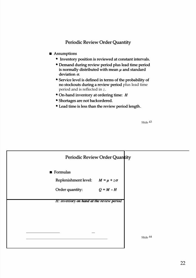
Periodic Review Order QuantityPeriodic Review Order Quantity
AssumptionsAssumptions
•• Inventory position is reviewed at constant intervals.Inventory position is reviewed at constant intervals.
•• Demand during review period plus lead time periodDemand during review period plus lead time periodis normally distributed with meanis normally distributed with mean µ µ and standardand standarddeviationdeviation σ σ ..
•• Service level is defined in terms of the probability ofService level is defined in terms of the probability ofnono stockoutsstockouts during a review periodduring a review period plus lead timeperiod and is reflected in z.
•• OnOn
--hand inventoryhand inventory
at ordering time:at ordering time: H H
•• Shortages are not backordered.Shortages are not backordered.
•• Lead time is less than the review period lengthLead time is less than the review period length..
44Slide
FormulasFormulas
Replenishment level:Replenishment level: M M == µ µ ++ z zσ σ
Order quantity:Order quantity: QQ == M M –– H H
H: inventory on hand at the review period H: inventory on hand at the review period
Periodic Review Order QuantityPeriodic Review Order Quantity
8/2/2019 Or B Inventory Models
http://slidepdf.com/reader/full/or-b-inventory-models 23/25
23
45Slide
Example: Ace BrushExample: Ace Brush
Periodic Review Order Quantity ModelPeriodic Review Order Quantity Model
•• Joe Walsh is a salesman for the Ace Brush Company. Joe Walsh is a salesman for the Ace Brush Company.
•• EveryEvery three weeksthree weeks he contacts Dollar Departmenthe contacts Dollar DepartmentStore so that they may place an order to replenishStore so that they may place an order to replenishtheir stock.their stock.
•• Weekly demand for Ace brushes at DollarWeekly demand for Ace brushes at Dollarapproximately follows a normal distribution with aapproximately follows a normal distribution with a
mean ofmean of
60 brushes and a standard deviation of 960 brushes and a standard deviation of 9
brushes per week.brushes per week.
46Slide
Example: Ace BrushExample: Ace Brush
Periodic Review Order Quantity ModelPeriodic Review Order Quantity Model
Once Joe submits an order, the lead time untilOnce Joe submits an order, the lead time untilDollar receives the brushes isDollar receives the brushes is one weekone week..
Dollar would like at most a 2% chance of runningDollar would like at most a 2% chance of running
out of stock during any replenishment period.out of stock during any replenishment period.
If Dollar has 75 brushes in stock when JoeIf Dollar has 75 brushes in stock when Joecontacts them, how many should they order?contacts them, how many should they order?
8/2/2019 Or B Inventory Models
http://slidepdf.com/reader/full/or-b-inventory-models 24/25
24
47Slide
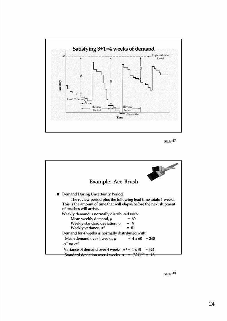
Satisfying 3+1=4 weeks of demandSatisfying 3+1=4 weeks of demand
48Slide
Example: Ace BrushExample: Ace Brush
Demand During Uncertainty PeriodDemand During Uncertainty Period
The review period plus the following lead time totals 4 weeks.The review period plus the following lead time totals 4 weeks.This is the amount of time that will elapse before the next shipThis is the amount of time that will elapse before the next shipmentmentof brushes will arrive.of brushes will arrive.
Weekly demand is normally distributed with:Weekly demand is normally distributed with:Mean weekly demand,Mean weekly demand, µ µ = 60= 60
Weekly standard deviation,Weekly standard deviation, σ σ = 9= 9Weekly variance,Weekly variance, σ σ 22 = 81= 81
Demand for 4 weeks is normally distributed with:Demand for 4 weeks is normally distributed with:
Mean demand over 4 weeks,Mean demand over 4 weeks, µ µ = 4 x 60 = 240= 4 x 60 = 240
σ σ 22 =n=n σ σ ‘‘22
Variance of demand over 4 weeks,Variance of demand over 4 weeks, σ σ 22 = 4 x 81 = 324= 4 x 81 = 324
Standard deviation over 4 weeks,Standard deviation over 4 weeks, σ σ = (324)= (324)1/21/2 = 18= 18
8/2/2019 Or B Inventory Models
http://slidepdf.com/reader/full/or-b-inventory-models 25/25
49Slide
Replenishment LevelReplenishment Level
M M == µ µ ++ z zσ σ
•• z: wherez: where z z is determined by the desiredis determined by the desired stockoutstockout probability.probability.For a 2%For a 2% stockoutstockout probability (2% tail area),probability (2% tail area), z z = 2.05.= 2.05.
•• µ µ , , σ σ determined in the previous slidedetermined in the previous slide
M M = 240 + 2.05(18) = 277 brushes= 240 + 2.05(18) = 277 brushes
As the store currently has 75 brushes in stock, Dollar shouldAs the store currently has 75 brushes in stock, Dollar shouldorder: 277order: 277 -- 75 = 202 brushes75 = 202 brushes
The safety stock is:The safety stock is: z zσ σ = (2.05)(18) = 37 brushes= (2.05)(18) = 37 brushes
Example: Ace BrushExample: Ace Brush
Related Documents