opus4.kobv.de · The spatiotemporal master equation: approximation of reaction-diffusion dynamics via Markov state modeling Stefanie Winkelmanna and Christof Schutte¨a,b aZuse Institute

Takustr. 714195 Berlin

GermanyZuse Institute Berlin

STEFANIE WINKELMANN1, CHRISTOF SCHUTTE2

The spatiotemporal master equation:approximation of reaction-diffusion dynamics via

Markov state modeling 3

1Zuse Institute Berlin (ZIB), Germany, [email protected] of Mathematics, Freie Universitat Berlin and Zuse Institute Berlin (ZIB), Germany,

[email protected] appear in: 2017

ZIB Report 16-60 (November 2016)

Zuse Institute BerlinTakustr. 714195 BerlinGermany

Telephone: +49 30-84185-0Telefax: +49 30-84185-125

E-mail: [email protected]: http://www.zib.de

ZIB-Report (Print) ISSN 1438-0064ZIB-Report (Internet) ISSN 2192-7782

The spatiotemporal master equation: approximation ofreaction-diffusion dynamics via Markov state modeling

Stefanie Winkelmanna and Christof Schuttea,b

aZuse Institute Berlin (ZIB), GermanybDepartment of Mathematics, Freie Universitat Berlin, Germany

AbstractAccurate modeling and numerical simulation of reaction kinetics is a topic of steady interest.

We consider the spatiotemporal chemical master equation (ST-CME) as a model for stochasticreaction-diffusion systems that exhibit properties of metastability. The space of motion is decom-posed into metastable compartments and diffusive motion is approximated by jumps betweenthese compartments. Treating these jumps as first-order reactions, simulation of the resultingstochastic system is possible by the Gillespie method. We present the theory of Markov statemodels (MSM) as a theoretical foundation of this intuitive approach. By means of Markov statemodeling, both the number and shape of compartments and the transition rates between themcan be determined. We consider the ST-CME for two reaction-diffusion systems and compare itto more detailed models. Moreover, a rigorous formal justification of the ST-CME by Galerkinprojection methods is presented.

1 Introduction

A reaction network is a system involving several chemical species undergoing multiple reactions.Depending on the particle concentration and mobility, different mathematical models are appropri-ate. In the case of rapid diffusion, the spatial position of the particles becomes negligible and thesystem may be considered as well-mixed. Then, the state of the system is defined by the numberof particles of each species and the dynamics are modeled by a continuous-time Markov chain withthe reactions described by jumps of the chain.[1] A characterization of the process is given by thechemical Master equation (CME) which describes the temporal evolution of the probabilities for thesystem to occupy each different state. Numerical methods for solving the CME are usually basedon Monte Carlo simulations of the underlying Markov jump process, such as Gillespie’s stochasticsimulation algorithm and its variants.[9, 12, 13, 14, 15] In the limit of high population concen-trations (large copy numbers for all species) the dynamics can be approximated by mass actionkinetics,[21] leading to a deterministic system described by ordinary differential equations.

In biological applications, the well-mixed assumption of the CME is often inadequate due tospatial inhomogeneities or limited speed of the diffusive motion of the particles. In this case, ahigher resolution in space is required leading to microscopic particle-tracking methods. The mostdetailed standard model is given by particle-based reaction-diffusion dynamics (PBRD) where allindividual particle paths and reaction events are explicitly resolved in time and space. Particles are

1

modeled as points (or spheres) in space undergoing Brownian motion. Bimolecular reactions takeplace with a certain probability per unit of time when two reactive particles meet within a predefinedreaction radius of each other.[2, 26, 32] An overview of the existing simulation tools for such detaileddynamics is given in Ref. 27. Simulations of PBRD-systems are based on time-discretizations. Ineach time step, the positions of all particles are advanced, followed by a check-up for adjacentreactive particles whose reaction radii overlap such that a reaction could fire. This scheme becomesinefficient when parts of the system are dense, because those parts then continuously stop the clock,i.e., require extremely small discretization time steps.

As an alternative there exist finite volume approaches where the state space is discretized into acollection of nonoverlapping cells and diffusion is approximated by a continuous-time random walkbetween the cells.[10, 17, 18, 20] A common choice for the discretization is a uniform Cartesian lat-tice, however, there also exist approaches with other types of meshes, e.g. consisting of triangles.[8]Bimolecular reactions occur with a fixed probability per unit of time between reactive particles sit-uated in the same cell. The state of the system is given by the number of particles of each speciesin each cell and the dynamics are described by the so-called reaction-diffusion master equation(RDME) which is formally a CME but with the states having a spatial interpretation. Diffusion ismodeled by first-order reactions, allowing each particle to change its position by switching betweencells. In this kind of approach the question of how to choose the mesh size in order to guaranteea small approximation error is of central importance. In fact, a fine discretization of space doesnot naturally lead to a high approximation quality because encounters of particles within the same(small) cell become unlikely such that bimolecular reactions are suppressed.[16, 18] In order toovercome this problem, the convergent RDME has been developed which allows particles to reactalso when being in nearby cells.[19]

In such a space discretization by a mesh with uniform size of the cells, all areas of the space areequally treated, irrespectively of the structural properties of the reaction-diffusion system. However,in many applications the diffusive and reactive properties of the system naturally exhibit certainstructural properties which suggest a more flexible and non-uniform coarse-graining. Especiallysituations of metastable diffusion dynamics propose to coarse-grain space into areas of metastability.Such situations will be considered in this article. An evident example is given by the process ofgene expression within an eukaryotic cell where some of the involved reactions (e.g. production ofmessenger RNA) take place only in the nucleus of the cell while others (e.g. production of proteins)are restricted to the cytoplasm, and transitions between these two compartments are relativelyrare in time. In this case, a description on the level of a CME (assuming well-mixed behaviorin total space) is obviously not appropriate, however, a split-up of space into two compartments(nucleus and cytoplasm) with diffusive transitions described by jumps might be enough to capturethe dynamics.

Although such a coarse-graining with only a few compartments which are chosen in consider-ation of the dynamical properties of the system seems natural, its mathematical background hasnot yet been examined. In this article, we describe the theoretical foundation of this approach andpresent practical methods to infer a reasonable splitting of space as well as corresponding transitionrates between the compartments out of experimental data or numerical simulations. The centralidea is to apply the theory of Markov state models (MSM) which proposes a scheme to constructcoarse-grained representations of conformational molecular kinetics. The existence of metastable

2

sets within the dynamics can be exploited to provide good approximation properties of the re-duced model on long timescales.[30] Instead of conformational dynamics of an individual moleculewe consider the total reaction-diffusion system and approximate the diffusion dynamics of eachmolecule by a jump process between the metastable compartments. With the jumps understoodas first-order reactions and the state of the total system given by the number of particles in eachof the compartments, the total dynamics are again characterized by a CME with spatial inter-pretation, which in this context will be called spatiotemporal CME (ST-CME). The ST-CME isformally conform with the RDME, but the underlying coarse-graining of space follows a completelydifferent concept, adapting the natural properties of the process and leading to an incomparablylower number of compartments. Typical compartments are not “small” such that the problem ofsuppressed second-order reactions, which appears for the RDME in the case of a small mesh size,is circumvented in the setting of the ST-CME.

As a prototypical example we will investigate reaction-diffusion systems within an eukaryote,where the split-up into nucleus and cytoplasm is quite obvious. However, the theory of MSM’s alsoenables to find number and geometry of compartments in cases where they are not known a priori.The resulting simplified models are readily understood and easy to interpret. By inferring thespatial clustering and the transition rates from experimental data, particle-based simulations arecompletely circumvented and trajectories of the total system can directly be generated by Gillespiesimulations of the derived ST-CME. Even if - for lack of experimental data - the MSM-constructionrequires simulations of the diffusion dynamics, the numerical complexity is reduced to a large extendbecause only the motion of an individual particle (and not the total population affected by reactionand diffusion) has to be produced.

In this paper, the ST-CME is viewed as an approximation of microscopic particle-based dy-namics with the spatial resolution reduced to the minimum possible degree, still maintaining thecharacteristic properties of the dynamics. Beside the intuitive, heuristic derivation, we give a con-crete mathematical justification showing that the ST-CME results from a Galerkin projection ofthe corresponding particle-based dynamics. Again inspired by MSM theory, this permits to deriveexplicit formulas for the model parameters depending on the microscopic variables.

In Section 2 the ST-CME is introduced as a reaction-diffusion model with adapted spatialresolution. The construction of the underlying MSM is described, explaining the procedure ofspace decomposition and the estimation of transition rates. Two examples are presented in orderto illustrate the approach. In Section 3, we analytically derive the ST-CME for a reduced reactionsystem by applying the Galerkin projection method to the corresponding particle-based dynamicalsystem. In the first step we consider a simplified model with not more than two particle species;the more general analysis for larger numbers of species and particles is given in the Appendix.

2 Modeling reaction-diffusion processes for metastable diffusion

In the following we first review some basic approaches to model reaction-diffusion processes on astochastic level. The spatiotemporal master equation is presented as a model with an intermediatespatial scaling, adapted to the natural properties of the system of interest. Then, in Section 2.2,we give a short introduction to the theory of Markov state models and apply it to determine thespatial coarse-graining and the jump parameters appearing in the ST-CME. Section 2.3 comprises

3

two illustrative examples to compare the approaches.

2.1 Modeling reaction-diffusion processes

We consider a set of particles moving in a compact domain Ω ⊂ Rd by continuous diffusion. Theparticles belong to different species Sl, l = 1, ..., L, and may interact with each other throughdifferent reaction channels Rk, k = 1, ...,K.

Particle-based reaction-diffusion (PBRD)

In the most detailed model of particle-based reaction-diffusion dynamics, the motion of every in-dividual particle is resolved in time and space. Positions of particles are represented as points orspheres undergoing Brownian motion, and bimolecular reactions occur with a certain microscopicreaction rate as soon as the particles are located within a predefined reaction radius of each other(Doi-model).[2, 7, 32] These systems cannot be explicitly solved but must be sampled by stochasticrealizations. Time is discretized, and for each time step the positions of all individual particles areadvanced according to a given rule of motion. Each advance is followed by a checkup for reactivecomplexes, i.e. sets of reactive particles whose reaction radii overlap. Given such a complex, thereaction can fire; whether this happens or not is decided randomly based on microscopic reactionrate. Further methods have been developed in order to include interaction potentials betweenparticles.[26] These permit effects such as space exclusion, molecular crowding and aggregation tobe modeled.The particle-based resolution is appropriate in cases of low particle concentrations and slow diffu-sion. Spatial inhomogeneities can be taken into account up to a very detailed level. The simula-tions, however, can be extremely costly often requiring several CPU-years in a single simulation forreaching the biological relevant timescales of seconds. If part of the system is dense, the approachbecomes numerically inefficient because reactions would fire in every iteration step. In such a case,a description of the population by concentrations is more appropriate, leading to PDE formulationsof the dynamics. For low concentration but rapid diffusion over the total space, the high spatialresolution becomes redundant and the system can to be modeled by the chemical master equation(CME).

The chemical master equation (CME)

In the case of rapid diffusion in a homogeneous environment, the system can be considered as well-mixed such that only the number of particles of each species is relevant while their spatial position isneglected. Let N(t) = (N1(t), ...,NL(t)) denote the state of the system at time t ≥ 0, with N l(t)referring to the number of particles of species Sl at time t. Given the stateN(t) = n = (nl)l=1,...,L ∈NL0 of the system, a reaction is described by transitions of the form n → n + νk with the integervector νk =

(ν1k , ..., ν

Lk

)giving the change in the number of particles of each species due to reaction

Rk. E.g., the chemical reaction 2Sl → Sl′ is described by the vector νk with νlk = −2, νl′k = 1 andzeros elsewhere. For each reaction Rk, a propensity function αk(n) defines the probability per unitof time for the reaction to occur given that N(t) = n. According to the law of mass action, thepropensity is a function of the corresponding macroscopic rate constant γk > 0 and the number of

4

particles involved in the reaction: For a unimolecular reaction by species l it holds αk(n) = γk ·nl;for a second-order reaction by two species l, l′, l 6= l′ one has αk(n) = γk · nl · nl′ .[1, 22] WithP (n, t) = P (N(t) = n|N(0) = n0) denoting the probability for the system to be in state n at timet, the dynamics are characterized by the chemical Master equation

dP (n, t)dt

=K∑k=1

(αk(n− νk)P (n− νk, t)− αk(n)P (n, t)

).

Realizations of the underlying Markov jump process can be created by Gillespie simulations.

The spatiotemporal chemical Master equation (ST-CME)

There exist many applications where the well-mixed assumption required for the chemical Masterequation is not fulfilled. Instead, diffusion of particles might be limited by local barriers in space,or the environment Ω offers inhomogeneities with respect to reaction propensities. An examplethat will be investigated in Section 2.3 describes the setting of diffusion within a eukaryotic cellwhich naturally decomposes into two compartments, the nucleus and the cytoplasm. By a reducedpermeability of the nuclear membrane, the diffusive flow through the cell is restricted such thata description by a chemical master equation would fail. Within each of the two compartment,however, the dynamics can indeed be considered as well-mixed, which motivates to consider thechemical Master equation on the level of compartments.

Such situations (in which the space Ω exhibits a particular structure with respect to the diffusionand reaction properties) will be considered here. More precisely, we make the following centralassumption.

Assumption 2.1. There is a decomposition of Ω into compartments Ωr, r = 1, ...,M , such that

1. transitions between compartments are rare (metastability),

2. within each compartment Ωr diffusion is rapid compared to reaction (well-mixed-property),

3. within each compartment the reaction rates are constant, i.e. independent of the position(homogeneity).

The first point of Assumption 2.1 delivers the basis for a construction of a Markov state modelfor the diffusive part of the reaction-diffusion network. With the diffusion processes of all particlesbeing metastable with respect to the same space decomposition, they can be approximated byMarkov jump processes on the fixed set of compartments Ωr : r = 1, ...,M. Within the ST-CME,the jumps are treated as first order reactions. By the second and third point of Assumption 2.1 wemake sure that within each compartment the reaction dynamics can accurately be described by achemical master equation.

Let N lr(t) denote the number of particles of species l in compartment r at time t. We take

N r(t) = (N1r (t), ..., NL

r (t)) to denote the state of present species in compartment r. The totalstate of the system at some point in time t is given by the matrix N(t) = (N r(t))r=1,...,M ∈ NM,L

0 .

5

Changes of the state are induced by diffusive transitions (jumps) between the compartments andby chemical reactions.

A jump of a particle of species l from compartment r to compartment s 6= r is described by atransition of the form

N →N +Els −El

r

where Elr is a matrix whose elements are all zero except the entry (r, l) which is one. Let λlrs

denote the jump rate for each individual particle of species l. Since all particles are assumed todiffuse independently of each other, the total probability per unit of time for a jump of species lfrom compartment r to s at time t is given by λlrsN l

r(t).For each of the reactions Rk, let again νk =

(ν1k , ..., ν

Lk

)describe the change in the number

of copies of all species induced by this reaction. Reaction Rk occurring in the r’th compartmentrefers to the transition N r(t) → N r(t) + νk. In order to specify where the reaction takes place,the vector νk is multiplied by a column vector er with the value 1 at entry r and zeros elsewhere.This gives a matrix erνk whose r’th row is equal to νk while all other rows contain zeros. Withthis notation, the change in the total state N due to reaction Rk taking place in compartment r isgiven by

N →N + erνk.

The propensity for such a reaction to occur is given by the function αkr (n) denoting the probabilityper unit of time for reaction Rk to occur in compartment r given that N r(t) = nr, i.e. it dependsαkr (n) only on the values of n referring to compartment r. Note that the rate constants whichdetermine the reaction propensities may depend on the compartment such that - in contrast to theCME - spatial inhomogeneities in the reaction propensities can be taken into account.

As in the setting of the CME, let

P (n, t) = P (N(t) = n|N(0) = n0)

be the probability that the process is in state n at time t given an initial state N(0) = n0. Thespatiotemporal chemical master equation (ST-CME) is then given by

dP (n, t)dt

=M∑r=1

∑s 6=r

L∑l=1

(λlsr(nls + 1)P (n+El

s −Elr, t)− λlrsnlrP (n, t)

)(1)

+M∑r=1

K∑k=1

(αkr (n− erνk)P (n− erνk, t)− αkr (n)P (n, t)

),

where the first line refers to the diffusive part (the transitions between the compartments) whilethe second line describes the chemical reactions within the compartments.

Numerical realizations of the ST-CME can again be created using the Gillespie method. Com-pared to particle-based simulations in which the trajectory of each single particle has to be cal-culated, the simulations of the ST-CME are computationally less expensive. However, due to thespatial interpretation, the state space of the ST-CME is larger than the one of the CME.

Remark 2.2. A reaction-diffusion Master equation (RDME) is formally identical to (1) but dif-ferent regarding the spatial discretization. In a RDME the underlying space Ω is discretized by a

6

structured or unstructured mesh leading to a large number mesh cells so that the first line of (1)in case of a RDME model is based on a discretization of the Laplacian operator underlying thediffusion process.[8, 11, 20]

To determine a convenient space discretization as well as suitable jump rates is the fundamentalissue for the representation of a reaction-diffusion system in terms of a ST-CME. It can be handledby constructing a Markov state model for the space of motion.

2.2 Spatial discretization via Markov state modeling

The theory of Markov state models (MSM’s) is a well established tool to approximate complexmolecular kinetics by Markov chains on a discrete partition of the configuration space.[4, 23, 24,25, 30, 29] The underlying process is assumed to exhibit a number of metastable sets in which thesystem remains for a comparatively long period of time before it switches to another metastableset. A MSM represents the effective dynamics of such a process by a Markov chain that jumpsbetween the metastable sets with the transition rates of the original process. Two main steps areessential for this approach: the identification of metastable compartments and the determinationof transition rates between them. Both steps are extensively studied in the literature, providingconcrete practical instructions.[4, 3, 5] Although usually interpreted in terms of conformationaldynamics, the approaches can directly be transferred to the kinetic dynamics of individual particleswithin a reaction-diffusion system. Within the ST-CME, jumps and reactions are uncoupled fromeach other and memoryless in the sense that a reaction taking place does not influence the jumppropensity of any species, and the reaction rates within each compartment are independent of theprevious evolution of the system. Thereby, a separate analysis of the diffusion properties is justified.In the following, we apply the MSM-theory to the pure diffusion process of an individual particle,fading out its interaction with other particles by reactions.

Spatial coarse-graining

Assuming that the space of motion consists of metastable areas where the reaction-diffusion dy-namics can be considered to be well-mixed, the first task is to identify the location and shape ofthese areas. While in certain applications the spatial clustering might be obvious (like e.g. for theprocess of gene expression), others will require an analysis of available data (either from simulationsor experiment) to define the number and geometry of compartments.

The MSM approach to perform this step of space decomposition is based on a two-stage processexploiting both geometry and kinetics.[4, 5, 28] Starting with a geometric clustering of space intosmall volume elements, the kinetic relevance of this clustering is checked for the given simulationdata, followed by a merging of elements which are kinetically strongly connected. As a concreteexample we shortly sketch the automatic state decomposition algorithm introduced in Ref. 5: Theiteration alternates between a split step (splitting the space into microstates) and a lump step(lumping microstates together to get macrostates with maximum possible metastability). Eachmakrostate is subsequently again fragmented into microstates, which are lumped again to redefinethe macrostates. By this alternation, the boundaries between macrostates are iteratively refined.The splitting is based on geometric criteria, while the lumping considers kinetic aspects, takingmetastability as a measure.

7

To illustrate the relevance of both geometric and kinetic aspects for the space discretization, onecan consider the example of nuclear membrane transport: By the reduced permeability of the nu-clear membrane, the cell decomposes into two metastable regions (nucleus and cytoplasm). A smallgeometric distance between two points is a first indication for belonging to the same compartment,however, this would also group together close points which are located on different sides of the nu-clear membrane and are thereby kinetically distant. While other clustering methods might fail tocapture the kinetic properties of the system under consideration, the MSM approach incorporatesthe relevant kinetic information and allocates such points into different compartments.[3]

The theoretical foundation of Markov state modeling comprises the spectral analysis of thetransfer operator which describes how the process propagates functions in state space over time.The dominant eigenvalues refer to long implied time scales, with the associated eigenvectors givinginformation about the metastable areas in space and the aggregate transition dynamics betweenthem. The algorithms used for spatial clustering by MSM’s require the availability of large amountof data sets. Transitions between metastable sets are infrequent events which even in long (butfinite) trajectories might be small in number. Fortunately, for MSM’s there exist methods tovalidate the model and to quantify the statistical error, allowing to rerun simulations in case ofhigh uncertainty (so called adaptive sampling).[4, 23, 25] The development of standards for thenumber and length of simulations needed for a statistically reliable modeling is in progress.[5]

Estimation of transition rates

Once a suitable space partitioning for the problem under consideration is given (known in advanceor determined by Markov state modeling as described before), the rates for transitions between thecompartments have to be estimated. The theory of MSM also delivers concrete practical techniquesto determine the transition rates out of trajectory data. Applied to the diffusion dynamics of aparticle in space, the rate estimation can shortly be summarized as follows.

Let the space Ω of motion be decomposed into compartments Ωr, r = 1, ...,M , with⋃Mr=1 Ωr = Ω

and (intΩr ) ∩ (intΩs) = ∅ for all r 6= s where intΩr denotes the interior of Ωr. The diffusion of asingle particle in Ω is given by a homogeneous, time-continuous Markov process (Xt)t≥0 with Xt

denoting the position of the particle in Ω at time t ≥ 0. We assume that (Xt) has a unique, positiveinvariant probability measure µ on Ω. Fixing a lag time τ > 0, the MSM process is a discrete-timeMarkov chain (Xn)n∈N on 1, ...,M with transition probabilities

Prs = Pµ(Xτ ∈ Ωs|X0 ∈ Ωr) (2)

where the subscript µ indicates that X0 ∼ µ. The Markov process (Xn) serves as an approximationof the process (Xn) defined by Xn = r ⇔ Xn·τ ∈ Ωr which, in general, is itself not Markovian buthas a memory. For details about the approximation quality see Ref. 25.

Given a trajectory (x0, x1, ..., xN ) of the diffusion process (Xt)t≥0 with xn = Xn·∆t for a fixedtime step ∆t > 0 (given from experimental data or separated simulation), the transition matrixP is estimated by counting the transitions between the compartments: Let the lag time τ = l∆t(l ∈ N) be a multiple of ∆t and set

Prs = Crs∑s′ Crs′

, Crs =N−l∑n=0

χr(xn)χs(xn+l) (3)

8

with χr denoting the indicator function of Ωr. Then P is a maximum-likelihood estimator for thetransition matrix P .[23, 24]

In order to turn from discrete time to continuous time within the coarse-grained setting, thematrix estimation is repeated for a range of lag times τ and the resulting transition matrices Pτ areused to determine appropriate transition rates λrs > 0 between the compartments in the setting of acontinuous-time Markov jump process. More precisely, we aim for a rate matrix Λ = (λrs)r,s=1,...,Mwith λrs > 0 for r 6= s and λrr = −

∑s 6=r λrs which describes the time-evolution of a memoryless

system by the master equationdpTtdt

= pTt Λ (4)

where pt(r) denotes the probability for the diffusion process to be in compartment r at time t.[31]With p0 denoting the initial distribution, the solution to (4) is given by pTt = pT0 e

Λt which suggeststhe relation Pτ ≈ eΛτ . On short time scales, the “true” process (Xt)t≥0 cannot be accuratelyapproximated by such a memoryless system because recrossings between the compartments inducememory effects.[6] For τ not too small, however, it indeed holds [4, 30]

1τ

log(Pτ ) ≈ constant

such that we can set Λ = 1τ log(Pτ ). The entries of the matrix Λ are the jump rates appearing in

the ST-CME. The discretization error arising with the coarse-graining can even be quantitativelybounded.[4]

Remark 2.3. The estimation of the rate matrix can be made more accurate by forcing it to fulfillcertain side constraints like detailed balance or the keep of an equilibrium distribution which isknown a priori.[4]

2.3 Illustrative Examples

For an illustration we consider two different reaction-diffusion systems within the cell of an eukary-ote. The cell naturally decomposes into two compartments, the nucleus and the cytoplasm, withthe nuclear membrane exhibiting a reduced permeability which induces a metastability of the diffu-sion dynamics. The cellular membrane is assumed to be impermeable such that the cell’s exterioris out of interest. Particles are assumed to move independently and not to influence each other intheir crossing behavior. Reactions between particles can only take place if the particles are in thesame compartment. The cell is modeled in two dimensions as two concentric circles representingthe membranes of nucleus and cytoplasm.

The first system under consideration is a quite artificial binding-unbinding network which isused to compare the dynamics characterized by the ST-CME to the underlying particle-based dy-namics. The congruence of the quantitative evolution of the systems (in terms of average populationnumbers) is revealed. Then, the more applied setting of gene expression is investigated, comparingthe qualitative properties of the ST-CME system to those induced by a RDME with Cartesian gridas given in Ref. 20. Both examples illustrate the ability of the ST-CME to reproduce the dynamicsof more detailed and complex model descriptions.

9

2.3.1 Binding and unbinding

As a first example we formulate a very general reaction-diffusion system consisting of three speciesS1 = A,S2 = B,S3 = C which diffuse within the cell and undergo the binding and unbindingreactions

R1 : A+B −→ C, R2 : C −→ A+B. (5)

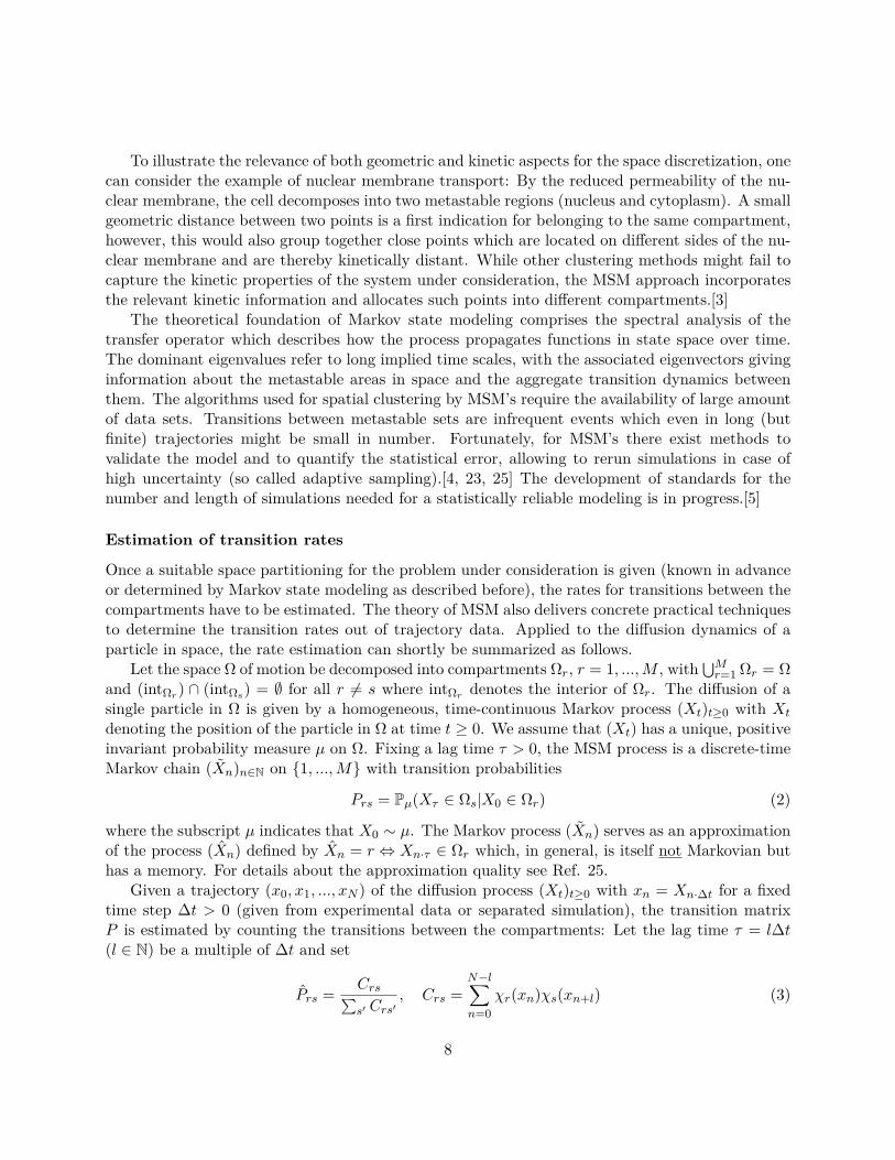
We assume that the binding reaction takes place only in the cytoplasm while unbinding is restrictedto the nucleus. This separation of reactions, combined with the metastability of diffusion due to areduced permeability of the nuclear membrane, obviously keeps the process from being well-mixedin total space, such that a description by a CME is not appropriate. A minimum spatial information- as it is given by a ST-CME - is needed to capture the characteristics of the dynamics. In thefollowing, we compare the ST-CME dynamics to appropriate particle-based dynamics where thediffusion of each particle is modeled by a process of Brownian motion with reflecting boundaryconditions at the cellular membrane and limited flux through the nuclear membrane, see Figure 1for an illustration.

-0.2 -0.1 0 0.1 0.2

-0.2

-0.1

0

0.1

0.2

Figure 1: Brownian motion on disk with metastable compartments. Brownian particlemoving on a disk (cell) containing a nucleus. The nuclear membrane exhibits a reduced permeability,rejecting most of the crossing trials of the trajectory.

Given the microscopic parameters of the system (i.e. diffusion constants, microscopic reactionrates and reaction radius for the Doi-model) as well as an initial population (we choose 5 A-particlesuniformly distributed in the nucleus and 5 B-particles uniformly distributed in the cytoplasm),numerical realizations of the particle-based reaction-diffusion system are produced by the Euler-Maruyama method. For all time-steps of a realization, the number of particles of each species ineach compartment is recorded. Then, a MSM for the diffusion process of each species is constructedas described in Section 2.2, yielding the jump rates between the two compartments necessary forthe ST-CME. The average binding time for two particles A and B within the cytoplasm is estimatednumerically in order to take its inverse for the macroscopic binding rate. Gillespie simulations ofthe resulting ST-CME give realizations of the total system on the spatially discretized level.

For both approaches (particle-based dynamics and ST-CME), the average evolution of the

10

population over time is estimated by Monte Carlo samples. In Figure 2 the results are shown, withan apparent consistency of both models.

0 0.1 0.2 0.3 0.4 0.50

0.5

1

1.5

2

2.5

3

3.5

4

4.5

5

ST-CME

PBRD

Cytoplasm

Nucleus

A

0 0.1 0.2 0.3 0.4 0.50

0.5

1

1.5

2

2.5

3

3.5

4

4.5

5

ST-CME

PBRD

Cytoplasm

Nucleus

B

0 0.1 0.2 0.3 0.4 0.50

0.5

1

1.5

2

2.5

3

3.5

4

4.5

5

ST-CME

PBRDC

Nucleus

Cytoplasm

Figure 2: Mean number of particles in conformation A (left), B (middle) and C (right) in thenucleus resp. the cytoplasm for separated reactions.

This binding-unbinding network will again be investigated in Section 3 where a formal derivationof the ST-CME is derived.

2.3.2 Gene expression

more applied setting is given by the process of gene expression by which information encodedin DNA is used for the production of functional proteins. This process is a complex network ofchemical reactions. In eukaryotes some of the involved reactions take place in the nucleus whileothers are restricted to the cytoplasm. On a very coarse level, the process can be described asfollows. In a first step, the gene is transcribed into messenger RNA (mRNA); this takes place inthe nucleus. The mRNA molecule is then exported to the cytoplasm where it is translated intoproteins. The proteins are imported into the nucleus where they can repress the gene, meaning thatits functionality in transcription is interrupted. Both mRNA and protein molecules are degradablein both compartments.Some of these steps contain themselves a complex series of chemical events. E.g., the crossing of thenuclear membrane by mRNA and protein molecules requires the assistance of import and exportreceptors because the pores of the nuclear membrane are too small for the molecules to pass throughby diffusion. For the ST-CME, such details are omitted and the crossing of the nuclear membraneis described by a single jump event with the jump rate chosen in a way to take account of all theinvolved steps. For many questions of interest a modeling on such a coarse level is appropriate.

In Ref. 20 the process of gene expression is analyzed in terms of the reaction-diffusion masterequation. With the cell and its nucleus also modeled by concentric circles, the space is discretizedby a regular 37 by 37 Cartesian mesh. Transitions of mRNA and proteins between nucleus andcytoplasm are modeled by binding and unbinding to export (resp. import) receptors which areassumed to be uniformly distributed throughout nucleus and cytoplasm at certain steady-stateconcentrations. After binding to the receptor the molecule can freely diffuse across the membrane.After this transition, the molecule has to unbind from the receptor before it can undergo furtherreactions. For the ST-CME the three steps (binding to receptor, transition, unbinding from re-ceptor) are merged and replaced by a jump event. In Ref. 20, simulations of the total system

11

show a periodicity in the total number of nuclear proteins. This periodicity is reproducible by theST-CME with only two compartments as will be demonstrated now.

Modeling for the ST-CME

The process of gene expression perfectly complies with the requirements of the ST-CME: Two ofthe reactions (transcription and translation) are restricted to certain areas of space, namely nucleusor cytoplasm. Transitions between these two compartments are of central relevance for the totaldynamics. Due to the complexity of membrane transition, the diffusion dynamics can be consideredas metastable. Within each compartment, local information is redundant and the dynamics can beconsidered as well-mixed.

More precisely, the following model is plausible. The transcription in the nucleus is given bythe reaction

DNAα1

r−→ DNA+mRNA

with the index r referring to compartment Ωr and α11 > 0 in the nucleus (= Ω1) while α1

2 = 0 inthe cytoplasm (= Ω2). Translation of mRNA into proteins P is given by

mRNAα2

r−→ mRNA+ P

with α21 = 0 in the nucleus and α2

2 > 0 in the cytoplasm. Repressing of DNA by a protein moleculerefers to the reaction

DNA+ Pα3

r−→ DNA∗,

where DNA∗ denotes the repressed DNA. Repressing is reversible by

DNA∗α4

r−→ DNA+ P.

Both mRNA and protein are degradable which is described by

mRNAα5

r−→ ∅

resp.P

α6r−→ ∅.

Transitions between nucleus and cytoplasm (possible for mRNA and protein molecules) are de-scribed by jumps with jump rates λmRNA12 > 0 (export of mRNA) and λP21 > 0 (import of protein).

In the RDME-formulation given in Ref. 20 most of these reactions are decomposed into severalsteps. Then, the protein production is shown to occur in bursts which is due to its repressingfunction: Given a large number of proteins, the repressing of the gene becomes very likely. If thegene is repressed, no new mRNA is transcribed, and the existing mRNA-molecules quickly vanishbecause of the large decay rate α5

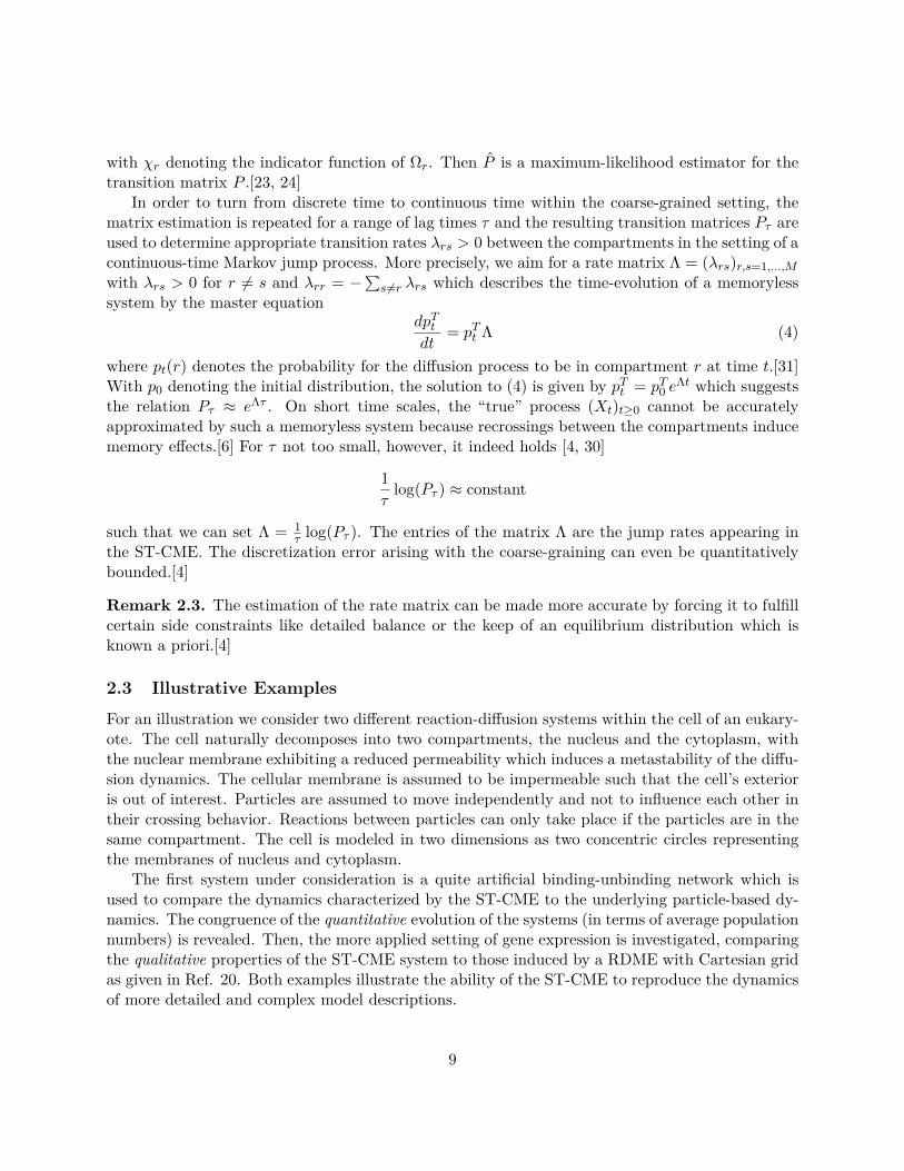
r . The translation into proteins is interrupted, and the proteinpopulation simply decays over time. With a smaller protein population, the repressing of the genebecomes less likely and transcription can start again. Such a periodic evolution of the numberof proteins exists in our coarse-grained model, see Figure 2.3.2 which looks much like Figure 8 in

12

Ref. 20. The chosen reaction rates roughly follow those given in Ref. 20, however without anyclaim to reproduce reality - we simply intend to maintain the fundamental qualitative behaviorof the system. Concretely, we set α1

1 = 0.05 (transcription in nucleus), α22 = 0.5 (translation

in cytoplasm), α31 = 0.01 (repressing in nucleus), α4

1 = 0.01 (reversal of repressing in nucleus),α5

2 = 0.3 (degradation of mRNA in the cytoplasm), α6r = 0.0025 (degradation of protein in both

compartments), λmRNA12 = λP21 = 0.4 (jump rates).

0 0.5 1 1.5 2

time×10 4

0

5

10

15

20

25

30

num

ber

of pro

tein

s

Figure 3: Number of nuclear proteins over time in one realization of the ST-CME. The proteinproduction occurs in bursts.

3 Formal derivation of the ST-CME for a reduced model

In Section 2.2 we presented the theory of Markov state models as a practical tool to significantlycoarsen the diffusion dynamics by finding suitable space decompositions as well as rates for transi-tions between the compartments. Beside the practical and algorithmic details, MSM’s also provide awell understood mathematical background, with the coarse-grained dynamics arising from Galerkinprojections of the original process.[30]

In this section, we apply the technical concepts and formally derive the ST-CME from a givenparticle-based model by means of a Galerkin approximation of the associated evolution equations.To this end, we study a reduced model consisting of two particles, one of species A and one ofspecies B, that diffuse independently in space Ω and undergo the binding reaction A + B → Cwith a position-independent rate γ1

micro when getting closer than ε1 > 0. The resulting C-particle

13

diffuses in space and can unbind again with a fixed rate γ2micro, compare the reaction system given

in (5). In this setting, the state space of the ST-CME reduces to states n ∈ NM,30 of either the

form n = E1r +E2

s - which refers to finding an A-particle in compartment Ωr and a B-particle incompartment Ωs while species C is absent - or n = E3

r referring to the existence of a C-particle incompartment Ωr while A and B are absent.

This is a totally over-simplified case that nevertheless allows to perform the formal derivationof the ST-CME in all details. As one can see in the Appendix, the approach can be transferred tolarger populations (particle and species numbers).

The particle-based model

As for the particle-based dynamics we make the following assumptions. Given A and B undergoinga reaction, the resulting C-particle is placed at the position x ∈ Ω of the A-particle. After anunbinding reaction, the particles A and B are placed within a ball Bε2(z) of radius ε2 > 0 aroundthe position z ∈ Ω of the preceding C-particle, with the positions x and y of A resp. B chosenindependently of each other, both uniformly distributed on Bε2(z).

We denote by p(x, y, t) the probability density for the particles A and B to be unbound andlocated at x resp. y at time t ≥ 0, and by p(z, t) the probability density for the particles to bebound with the C-particle located at z at time t ≥ 0. With this notation it holds∫

Ω2p(x, y, t) dxdy +

∫Ωp(z, t) dz = 1

for all times t ≥ 0.The time evolution of the two functions p and p is given by a coupled system of differential

equations:

∂tp(x, y, t) = (L1p)(x, y, t) + (L2p)(x, y, t) (6)−γ1

micro φε1(x, y)p(x, y, t)

+ γ2micro

|Bε2 |2∫φε2(x, z)φε2(y, z)p (z, t) dz,

∂tp(z, t) = (L3p)(z, t) (7)

+γ1micro

∫φε1(z, y)p(z, y, t) dy

−γ2micro p(z, t),

where L1, L2, L3 denote the generators of the diffusion processes of species A,B,C (in flat spaceswithout energy barriers these are Laplacian operators), respectively, and φεk

(k = 1, 2) is given by

φεk(x, y) = Φ

( |x− y|εk

)where Φ denotes the indicator function of the ball B1(0). In (6), outflow is induced by the bindingreaction in cases where the positions x and y are ε1-close to each other (2nd line), while inflow isinduced in case of an existing C-particle with its location being able to produce the given positions

14

x and y after unbinding (3rd line). In (7), binding induces inflow (2nd line) where the position ofthe former A-particle has to be at the given position z of the resulting C-particle, while unbindinginduces outflow (3rd line), compare the given placement assumptions.

Galerkin projection

The dynamics described by the coupled equations (6) and (7) have a full spatial resolution, breakingdown the exact positions of the particles in space. For the ST-CME the information must becoarsened to the level of compartments. This is done by projecting the dynamics onto a suitablelow-dimensional ansatz space.

We consider a partition of Ω into subsets Ωr, r = 1, ...,M , and denote by χr the indicatorfunction of Ωr. That is, χr is 1 inside of Ωr and 0 outside. Let 〈f, g〉 be the usual L2-scalar productof functions f and g that depend on Ω, i.e., 〈f, g〉 =

∫Ω f(x)g(x)dx. If the generators L1, L2, L3

do not denote flat diffusion but diffusion in an energy landscape, then the scalar product must beweighted with the respective product invariant measure, see Ref. 30. Define

µr = 〈1, χr〉

where 1 is the constant 1-function on Ω. The Galerkin projection Q : L2(Ω) → D onto thefinite-dimensional ansatz space D = spanχr : r = 1, ...,M is given by

Qv =M∑r=1

1µr〈χr, v〉χr, v ∈ L2(Ω).

We further use the functions

χrs(x, y) = χr(x)χs(y), r, s = 1, ...,M,

as a partition of unity of Ω× Ω. Parallel to the definitions before, we set

µrs = 〈1, χrs〉 ,

where in this context 〈·, ·〉 refers to the L2-scalar product on Ω× Ω, and

Qv =M∑

r,s=1

1µrs〈χrs, v〉χrs, v ∈ L2

(Ω2),

as a projection onto D = spanχrs : r, s = 1, ...,M. By definition it holds

µrs = µrµs.

Applying the projection to the density functions p and p gives the ansatz

(Qp)(x, y, t) =M∑

r,s=1prs(t)χrs(x, y),

15

(Qp)(z, t) =M∑r=1

pr(t)χr(z),

with time dependent coefficients prs(t) and pr(t). Inserting into (6) and (7) yields

M∑r,s=1

∂tprs(t)χrs(x, y) =M∑

r,s=1prs(t)

(L1χrs(x, y) + L2χrs(x, y)

)(8)

−γ1micro

M∑r,s=1

prs(t)φε1(x, y)χrs(x, y)

+ γ2micro

|Bε2 |2∑i

pi(t)∫φε2(x, z)φε2(y, z)χr(z) dz,

M∑r=1

∂tpr(t)χr(z) =M∑r=1

pr(t)L3χr(z) (9)

+γ1micro

M∑r,s=1

prs(t)∫φε1(z, y)χrs(z, y) dy

−γ2micro

M∑r=1

pr(t)χr(z).

The local coordinates x, y, z of the particles still appear as arguments. In order to eliminate them,the coupled equations (8) and (9) are themselves projected onto the given ansatz space, which refersto taking local averages of the terms for each combination of compartments. This automaticallydelivers the formal relation between the microscopic and the macroscopic model parameters. Infact, we define the macroscopic reaction rate constant for r, s, r′ = 1, ...,M by the averages

γ1rs := γ1

micro ·1µrs

∫χr(x)χs(y)φε1(x, y) dx dy,

γ2rsr′ := γ2

micro

|Bε2 |2· 1µr

∫χr(x)χs(y)χr′(z)φε2(x, z)φε2(y, z) dx dy dz,

which depend on the microscopic reaction rate and the reaction radius. Similarly, the jump ratesare given by

λlrs := 1µr

∫χs(x)Llχr(x) dx = 1

µr〈χs, Llχr〉 , l = 1, 2, 3.

Since Ll, l = 1, 2, only acts on xl, we have that

〈χrs, L1χr′s′〉 =µs 〈χr, L1χr′〉 = µr′sλ

1r′r for s = s′,0 otherwise,

〈χrs, L2χr′s′〉 =µr 〈χs, L2χs′〉 = µrs′λ

2s′s for r = r′,0 otherwise.

16

With this observation and the notations from above we get, by multiplication of (8) with 〈χrs, ·〉and by multiplication of (9) with 〈χr, ·〉, the system

µrs∂tprs(t) =M∑r′=1

λ1r′r · µr′spr′s(t) +

M∑s′=1

λ2s′s · µrs′prs′(t) (10)

−γ1rs · µrsprs(t) +

M∑r′=1

γ2rsr′ · µr′ pr′(t),

µr∂tpr(t) =M∑r′=1

λ3r′r · µr′ pr′(t) (11)

+M∑s=1

γ1rs · µrsprs(t)− γ2

micro · µrpr(t),

which does not contain any local coordinates, anymore. The system of equations (10) and (11) ac-tually can be understood as a spatiotemporal master equation, given the assumption that reactionsare also possible between particles suited in different compartments. With respect to the notationgiven in (1), we have the relation

P (n, t) =

µrs · prs(t) for n = E1

r +E2s,

µr · pr(t) for n = E3r ,

0 otherwise,

where P (n, t) is the probability to find the system in state n at time t, compare Section 2.1.In order to reveal the parallelism to the ST-CME given in (1), we assume that such “mixed”

reactions are suppressed. I.e., reactions take place only between particles located within the samecompartment and the product of a reaction is placed in the compartment of the reagents. Thisrefers to setting γ1

rs = 0, γ2rsr′ = 0 for all mixed (non constant) combinations of indices. For

comparatively large compartments and small ε1, ε2, all these values are close to zero for mixedindices by definition, anyway. For the reaction rate functions appearing in (1) we then obtain

α1r(n) =

γ1

micro|Bε1 |µr

for n = E1r +E2

r ,

0 otherwise,α2r(n) =

γ2

micro for n = E3r ,

0 otherwise.

Now, the equations simplify to

µrs∂tprs(t) =M∑r′=1

λ1r′r · µr′spr′s(t) +

M∑s′=1

λ2s′s · µrs′prs′(t)

−δrsγ1micro|Bε1 |µr· µrsprs(t) + δrsγ

2micro · µrpr(t),

µr∂tpr(t) =M∑r′=1

λ3r′r · µr′ pr′(t)

+γ1micro|Bε1 |µr· µrrprr(t)− γ2

micro · µrpr(t),

17

where δrs is the Kronecker delta. Noting that by definition it holds λlrr = −∑r′ 6=r λ

lrr′ for all

l = 1, 2, 3, this is just a reformulation of the ST-CME (1).

Remark 3.1. The available theory of Markov state models shows that one may also use ansatzfunctions χr that are different from indicator functions as long as they form a partition of unityof Ω.[30, 29] That is, along these lines we can also derive versions of the ST-CME where spatialdiscretization is not based on sets/compartments but on smooth functions, e.g. committor functionsfor core sets as in Ref. 29 or radial basis functions as in meshless discretization.[33] This increasesthe flexibility of our approach significantly and is known to allow for superior approximation qualityif recrossing scenarios are important.[30]

4 Conclusion

We introduced the spatiotemporal master equation as a framework for modeling reaction-diffusiondynamics in situations where the diffusion process exhibits metastability. By the construction of aMarkov state model for the diffusive part, the structural properties of the dynamics are preservedand diffusion is replaced by a jump process on a comparatively small set of compartments. Al-though in the literature usually related to conformational dynamics of an individual molecule, thetheory of MSM is a powerful tool for finding adequate space decompositions and estimating therelated transition parameters in a reaction-diffusion system of several molecules. In application, themethod can directly process experimental data such that particle-based simulations are completelycircumvented.

For the ST-CME approach to by valid, the well-mixed assumption does not have to applyfor the total dynamics (as it does for the CME) but only on the level of compartments. As forthe spatial resolution the ST-CME lies between the CME which excludes all spatial informationand more detailed models like the RDME (where space is discretized by meshes) or particle-basedreaction-diffusion systems (where the exact positions of all particles are retraced). The same istrue for the numerical effort induced by simulations of the respective systems. We compared themodels for two reaction-diffusion systems within an eukaryotic cell and showed that the ST-CMEis able to replicate the more detailed models regarding quantitative and qualitative properties.

Describing a reaction-diffusion system which behaves well-mixed in spatial subareas by a ST-CME is an intuitive approach. We showed that this approach has a clear mathematical foundation,with the ST-CME arising from a Galerkin projection of the corresponding particle-based dynamicalsystem onto the subspace spanned by appropriate ansatz functions. In the standard case, theseansatz functions are the indicator functions of the compartments, and the ST-CME is a combinationof a jump process between compartments and the reaction part. However, other families of ansatzfunctions may provide superior approximation properties. The analysis given in the Appendix showsthat, in principle, the ansatz functions used for the Galerkin approach could not only discretize thespatial domain but also particle number space. A detailed analysis of how to choose the ansatzfunctions is not given here but will have to be part of future research.

Another topic of interest is the combination of the different models in situations where partsof a system are well-mixed while others require a particle-based resolution. Then, the ST-CMEhas to be coupled to the stochastic dynamics of some particles that are individually tracked in

18

certain areas of space. In contrast, also parts of the system could show high density allowing fora description by ODE’s which leads to a stochastic-deterministic evolution equation comprisinga ST-CME. The development of such hybrid approaches to handle multi-scale reaction-diffusiondynamics is subject of ongoing work.

Acknowledgment

This research has been partially funded by Deutsche Forschungsgemeinschaft (DFG) through grantCRC 1114.

19

Appendix

In Section 3 we formally derived the ST-CME from a given particle-based model of binding andunbinding with not more than one particle of each species. We will here generalize the analysisto systems with larger populations: Several particles of species A and B diffuse independently inspace Ω and undergo the binding reaction A+B → C with a position-independent rate γ1

micro whengetting closer than ε1 > 0. The resulting C-particles diffuse in space and can unbind again with afixed rate γ2

micro.

Particle numbers: Subsequently we assume that we never have more than n particles of everyindividual type in our system. That is, if a, b, c denote the numbers of molecules of types A,B,Cin the system, then

(a, b, c) ∈ N , N = (a, b, c) : a, b, c ≤ n, , a+ b+ 2c ≤ 2n.

Notation: In addition to the given space of motion Ω we introduce the artificial void state Vindicating that the particle is absent. For every individual particle in the system the position thencomes from S = V × Ω. The positions of the n particles of type A are denoted by

X = (x1, . . . , xn) ∈ Sn,

and those of B and C by

Y = (y1, . . . , yn) ∈ Sn, Z = (z1, . . . , zn) ∈ Sn,

such that the state of the entire system is given by

(X,Y, Z) ∈ S3n.

In the following we consider only those (X,Y, Z) with(∑i

χΩ(xi),∑i

χΩ(yi),∑i

χΩ(zi))∈ N .

Placement assumption: Given the positions xi ∈ Ω and yj ∈ Ω of an A- and a B-particleundergoing a reaction, the resulting C-particle is placed at the position xi of the A-particle. Afteran unbinding reaction, the particles A and B are placed within a ball Bε2(z) of radius ε2 aroundthe position zk ∈ Ω of the preceding C-particle, with the positions xi and yj of A resp. B chosenindependently of each other, both uniformly distributed on Bε2(zk).

The index of a C-particle resulting from a binding reaction is chosen to be the first index of avoid state in Z. Equivalently, the positions of the A- and B-particles resulting from unbinding areinserted into X and Y at the respective first void entry. The insertion of a position x ∈ Ω at indexk into state X ∈ Sn is denoted by

X+k (x) = (x1, . . . , xk−1, x, xk+1, . . . , xn),

while setting position xk in state X ∈ Sn to void is denoted by

X−k = (x1, . . . , xk−1, V, xk+1, . . . , xn).

Equivalent notations are chosen for Y and Z.

20

The particle-based dynamics

By p(X,Y, Z, t) we denote the probability density function of finding the system in state (X,Y, Z) ∈S3n at time t. For integration we use the notation, for example,∫

Sp(x1, . . . , xn, Y, Z, t)dx1 = p(V, x2, . . . , xn, Y, Z, t) +

∫Ωp(x1, . . . , xn, Y, Z, t)dx1.

Let Lxi , Lyj , Lzkdenote the generators of the diffusion processes of species A,B,C acting on coor-

dinate xj , yj and zk on Ω, respectively. Then we define

LAp(x1, . . . , xn, Y, Z, t) =n∑i=1

χΩ(xi)Lxip(x1, . . . , xn, Y, Z, t).

The time evolution of the function p is given by the following differential equation:∂tp(X,Y, Z, t)

= (LA + LB + LC)p(X,Y, Z, t) (12)

−γ1micro

n∑i,j=1

χΩ(xi)χΩ(yj)φε1 (xi, yj)p(X,Y, Z, t)

+γ1micro

n∑k=1

k∏l=1

χΩ(zl)n∑

i,j=1

χV (xi)χV (yj)∫

Ωφε1 (zk, y)p

(X+

i (zk), Y +j (y), Z−

k, t)dy

−γ2micro

n∑k=1

χΩ(zk)p(X,Y, Z, t)

+γ2

micro|Bε2 |2

n∑k=1

χV (zk)n∑

i,j=1

i∏l=1

χΩ(xl)j∏

l=1

χΩ(yl)∫

Ωφε2 (xi, z)φε2 (yj , z)p

(X−i , Y

−j , Z+

k(z) , t

)dz

where φε is given byφε(x1, x2) = Φ

( |x1 − x2|ε

)with Φ denoting the indicator function of the ball B1(0).

Explanation:

• The first line in equation (12) refers to the independent diffusion of all particles.

• The second line refers to the outflow from state (X,Y, Z) induced by the binding reaction.

• The third line refers to the inflow induced by the binding reaction of the form(X+i (zk), Y +

j (y), Z−k)−→ (X,Y, Z).

For the state (X,Y, Z) to result from this reaction, the entry zk of Z has to be located in Ωand must fulfill zl ∈ Ω for all l < k because the new positions are assumed to be located atthe first index of a void state in Z. The actual positions xi and yj of X and Y have to bevoid, while before they are given by zk and y with y located in an ε1-environment around zk.

21

• The 4’th line refers to the outflow from (X,Y, Z) by unbinding.

• The 5’th line refers to the inflow induced by unbinding of the form(X−i , Y

−j , Z

+k (z)

)−→ (X,Y, Z).

Here, the actual position zk must be void, while the positions xi and yj both have to be in Ωwith no preceding void-entries (again because the new positions resulting from unbinding areplaced at the respective first void-entries). Both xi and yj must be ε2-close to the z-particlethey result from. As both positions are chosen uniformly distributed in the Bε2-ball aroundz, the unbinding rate is divided by its size squared.

Galerkin projection

Ansatz functions. We consider a partition of Ω into subsets Ω1, ...,Ωm and define the indicatorfunction for the system to have exactly ar ∈ 0, ..., n molecules of type A in set Ωr ⊂ Ω:

χar (X|Ωr) =

1 if∑ni=1 χr(xi) = ar,

0 otherwise,

where χr is the indicator function of Ωr. Then, the indicator function for having exactly ar moleculesof type A and br molecules of type B and cr molecules of type C in set Ωr (ar, br, cr ∈ 0, ..., n)is given by

χar,br,cr (X,Y, Z|Ωr) = χar (X|Ωr)χbr (Y |Ωr)χcr (Z|Ωr).

For the total system we use the ansatz functions

χa,b,c(X,Y, Z) =m∏r=1

χar,br,cr (X,Y, Z|Ωr)

where a = (ar)r=1,...,m, b = (br)r=1,...,m, c = (cr)r=1,...,m with ar, br, cr ∈ 0, ..., n and(m∑r=1

ar,m∑r=1

br,m∑r=1

cr

)∈ N .

The allowed index set of the three vector-indices of our ansatz functions will be denoted I. It isimportant to notice that these ansatz functions do not overlap,

〈χa,b,c, χa,b,c〉 = µa,b,c δaaδbbδcc, µa,b,c > 0,

but form a partition of unity of the accessible state space.

Galerkin ansatz. We consider the Galerkin projection Q : L2 (S3n) → D onto the finite-dimensional ansatz space D = spanχa,b,c : (a, b, c) ∈ I given by

Qv =∑

(a,b,c)∈I

1µa,b,c

〈χa,b,c, v〉χa,b,c, v ∈ L2(S3n

)

22

withµa,b,c = 〈1, χa,b,c〉

and〈u, v〉 =

∫S. . .

∫Su(X,Y, Z)v(X,Y, Z)dx1 . . . dxndy1 . . . dyndz1 . . . dzn.

The ansatz for p(X,Y, Z, t) now is

(Qp)(X,Y, Z, t) =∑

(a,b,c)∈Ipa,b,c(t)χa,b,c(X,Y, Z),

withpa,b,c(t) = 1

µa,b,c〈χa,b,c, p(·, t)〉.

Inserting into (12) gives∑(a,b,c)∈I

∂tpa,b,c(t)χa,b,c(X,Y, Z)

=∑

(a,b,c)∈I

pa,b,c(t)(LA + LB + LC)χa,b,c(X,Y, Z)

−γ1micro

∑(a,b,c)∈I

pa,b,c(t)n∑

i,j=1

χΩ(xi)χΩ(yj)φε1 (xi, yj)χa,b,c(X,Y, Z)

+γ1micro

∑(a,b,c)∈I

pa,b,c(t)n∑

i,j,k=1

k∏l=1

χΩ(zl)χV (xi)χV (yj)∫

Ωφε1 (zk, y)χa,b,c

(X+

i (zk), Y +j (y), Z−

k

)dy

−γ2micro

∑(a,b,c)∈I

pa,b,c(t)n∑

k=1

χΩ(zk)χa,b,c(X,Y, Z)

+γ2

micro|Bε2 |2

∑(a,b,c)∈I

pa,b,c(t)n∑

i,j,k=1

χV (zk)i∏

l=1

χΩ(xl)j∏

l=1

χΩ(yl)∫

Ωφε2 (xi, z)φε2 (yj , z)χa,b,c

(X−i , Y

−j , Z+

k(z))dz

Multiplication by⟨χa,b,c, ·

⟩gives

µa,b,c · ∂tpa,b,c(t)

=∑

(a,b,c)∈I

⟨χa,b,c, (LA + LB + LC)χa,b,c

⟩· pa,b,c(t)

−γ1micro

∑(a,b,c)∈I

⟨χa,b,c,

n∑i,j=1

χΩ(xi)χΩ(yj)φε1 (xi, yj)χa,b,c

⟩· pa,b,c(t)

+γ1micro

∑(a,b,c)∈I

⟨χa,b,c,

n∑i,j,k=1

k∏l=1

χΩ(zl)χV (xi)χV (yj)∫

Ωφε1 (zk, y)χa,b,c

(X+

i (zk), Y +j (y), Z−

k

)dy

⟩· pa,b,c(t)

−γ2micro

∑(a,b,c)∈I

⟨χa,b,c,

n∑k=1

χΩ(zk)χa,b,c

⟩· pa,b,c(t)

+γ2

micro|Bε2 |2

∑(a,b,c)∈I

⟨χa,b,c,

n∑i,j,k=1

χV (zk)i∏

l=1

χΩ(xl)j∏

l=1

χΩ(yl)∫

Ωφε2 (xi, z)φε2 (yj , z)χa,b,c

(X−i , Y

−j , Z+

k(z))dz

⟩· pa,b,c(t)

23

Due to the scalar product structure, most of the summands vanish. For the remaining summandswe choose the following notations:

α1(a, b, c) := γ1micro ·

1µa,b,c

∫ ∑i,j

χΩ(xi)χΩ(yj)φε1 (xi, yj)χa,b,c(X,Y, Z) dX dY dZ

α1rr′ (a, b, c) := γ1

micro ·1

µa,b,c

∫ n∑i,j,k=1

k−1∏l=1

χΩ(zl)χr(zk)χV (xi)χV (yj)∫

Ωr′

φε1 (zk, y)χa,b,c

(X+

i (zk), Y +j (y), Z−

k

)dy dX dY dZ

= γ1micro ·

1µa,b,c

∫ n∑i,j,k=1

k−1∏l=1

χΩ(zl)χV (zk)χr(xi)χr′ (yj)φε1 (xi, yj)χa,b,c (X,Y, Z) dX dY dZ

= γ1micro ·

1µa,b,c

∫ n∑i,j=1

χr(xi)χr′ (yj)φε1 (xi, yj)χa,b,c (X,Y, Z) dX dY dZ

which implies ∑r,r′

α1rr′(a, b, c) = α1(a, b, c)

for all a, b, c ∈ I, and

α2(a, b, c) := γ2micro ·

1µa,b,c

∫ ∑k

χΩ(zk)χa,b,c(X,Y, Z) dX dY dZ

α2rr′ (a, b, c) :=

γ2micro|Bε2 |2

·1

µa,b,c

∫ n∑i,j,k=1

χV (zk)i−1∏l=1

χΩ(xl)χr(xi)j−1∏l=1

χΩ(yl)χr′ (yj)

·∫

Ωr

φε2 (xi, z)φε2 (yj , z)χa,b,c

(X−i , Y

−j , Z+

k(z))dz dX dY dZ

=γ2

micro|Bε2 |2

·1

µa,b,c

∫ n∑i,j,k=1

χr(zk)i−1∏l=1

χΩ(xl)χr(xi)j−1∏l=1

χΩ(yl)χr′ (yj)

·φε2 (xi, zk)φε2 (yj , zk)χa,b,c

(X−i , Y

−j , Z

)dX dY dZ

=γ2

micro|Bε2 |2

·1

µa,b,c

∫ n∑i,j,k=1

χr(zk)i−1∏l=1

χΩ(xl)χV (xi)j−1∏l=1

χΩ(yl)χV (yj)

·∫

Ωr

∫Ωr′

φε2 (x, zk)φε2 (y, zk) dx dy · χa,b,c (X,Y, Z) dX dY dZ

=γ2

micro|Bε2 |2

·1

µa,b,c

∫ n∑k=1

χr(zk) · |Brε2 (zk)| · |Br′

ε2 (zk)| · χa,b,c (X,Y, Z) dX dY dZ

where|Br

ε2(z)| :=∫

Ωr

φε2(x, z) dx

such that∑mr=1 |Br

ε2(z)| = |Bε2 | for all z ∈ Ω and therefore∑r,r′

α2rr′(a, b, c) = α2(a, b, c)

24

for all a, b, c ∈ I.

For the diffusion part we have⟨χa,b,c, (LA + LB + LC)χa,b,c

⟩=

⟨χa,b,c, LAχa,b,c

⟩+⟨χa,b,c, LBχa,b,c

⟩+⟨χa,b,c, LCχa,b,c

⟩and ⟨

χa,b,c, LAχa,b,c⟩

=⟨χa,b,c,

n∑i=1

χΩ(xi)Lxiχa,b,c

⟩. (13)

In each of these summands, the generator only acts on the coordinates Xi of one individual particleof species A which means that the related scalar product can be nonzero only for those a, b, c witha = a+ 1r′ − 1r for some r, r′ ∈ 1, ...,m, while b = b and c = c. (In an equivalent notation, thisstatement holds for species B and C.)

We assume that all particles of one species follow the same diffusion dynamics (i.e. Lxi = L1for all i; equivalently for yi, zi). Then, for r, r′ = 1, ...,m and l = 1, 2, 3 we define the jump ratefrom Ωr′ to Ωr by

λlr′r := 1µr′〈χr, Llχr′〉

which - by the properties of the propagator Ll - fulfills λlr′r ≥ 0 for r′ 6= r and λlrr = −∑r′ 6=r λ

lrr′

for all r.

Fixing one xi (for simplicity i = 1) we have⟨χa,b,c, χΩ(x1)Lx1χa,b,c

⟩=

∑r

⟨χa,b,c, χr(x1)Lx1χa,b,c

⟩=

∑r

∫χa,b,c(X,Y, Z)χr(x1)(Lx1χa,b,c)(X,Y, Z) dX dY dZ

=∑

r: ar>0r′: ar′ >0

∫χr(x1)(Lx1χr′ )(x1)χa−1r (x2, ..., xn)χa−1r′ (x2, ..., xn)χb(Y )χb(Y )χc(Z)χc(Z) dX dY dZ

=∑

r: ar>0r′: ar′ >0

µr′λ1r′r · δa−1r′ ,a−1r

∫χa−1r (x2, ..., xn) dx2 ... dxn · δb,b µb · δc,c µc

=∑

r: ar>0r′: ar′ >0

δa−1r′ ,a−1r · δb,b · δc,c · λ1r′rµa+1r’ -1r,b,c.

In (13) we sum up over all i = 1, ..., n, which leads to a multiplication of λ1r′r by ar′ = (a+1r′−1r)r′

giving ⟨χa,b,c, LAχa+1r’ -1r,b,c

⟩=

∑r,r′

(a+ 1r′ − 1r)r′ · λ1r′r · µa+1r’ -1r,b,c

=∑r

ar · λ1rr · µa,b,c +

∑r′ 6=r

(ar′ + 1) · λ1r′r · µa+1r’ -1r,b,c

25

We finally get

µa,b,c · ∂tpa,b,c(t)

=∑r

∑r′ 6=r

(λ1r′r(ar′ + 1)µa+1r’ -1r,b,c

pa+1r’ -1r,b,c− λ1

rr′ arµa,b,cpa,b,c

)+∑r

∑r′ 6=r

(λ2r′r(br′ + 1)µa,b+1r’ -1r,c

pa,b+1r’ -1r,c− λ2

rr′ brµa,b,cpa,b,c

)+∑r

∑r′ 6=r

(λ3r′r(cr′ + 1)µa,b,c+1r’ -1r

pa,b,c+1r’ -1r− λ3

rr′ crµa,b,cpa,b,c

)−α1(a, b, c) · µa,b,c · pa,b,c(t)

+∑

r,r′:cr>0α1rr′(a+ 1r, b+ 1r’, c -1r) · µa+1r,b+1r’,c -1r

· pa+1r,b+1r’,c -1r(t)

−α2(a, b, c) · µa,b,c · pa,b,c(t)

+∑

r,r′:ar>0,br′>0α2rr′(a -1r, b -1r’, c+ 1r) · µa -1r,b -1r’,c+1r

· pa -1r,b -1r’,c+1r(t).

Setting α1rr′ = 0, α2

rr′ = 0 for r 6= r′, this is the ST-CME given in (1), where n is given by(a, b, c) with n1

r = ar, n2r = br, n3

r = cr and

P (n, t) = µa,b,c · pa,b,c(t)

for n = (a, b, c).

26

References

[1] D. F. Anderson and T. G. Kurtz. Continuous time markov chain models for chemical reactionnetworks. In Design and analysis of biomolecular circuits, pages 3–42. Springer, 2011.

[2] S. Andrews and D. Bray. Stochastic simulation of chemical reactions with spatial resolutionand single molecule detail. Physical Biology, 1(3):137, 2004.

[3] G. R. Bowman, X. Huang, and V. S. Pande. Using generalized ensemble simulations andmarkov state models to identify conformational states. Methods, 49(2):197–201, 2009.

[4] G. R. Bowman, V. S. Pande, and F. Noe. An introduction to Markov state models and theirapplication to long timescale molecular simulation. Advances in Experimental Medicine andBiology. Springer, 2014.

[5] J. D. Chodera, K. A. Dill, N. Singhal, V. S. Pande, W. C. Swope, and J. W. Pitera. Auto-matic discovery of metastable states for the construction of Markov models of macromolecularconformational dynamics. J. Chem. Phys., 126:155101, 2007.

[6] J. D. Chodera, P. J. Elms, W. C. Swope, J.-H. Prinz, S. Marqusee, C. Bustamante, F. Noe, andV. S. Pande. A robust approach to estimating rates from time-correlation functions. arXiv:1108.2304, August 2011.

[7] M. Doi. Stochastic theory of diffusion-controlled reaction. Journal of Physics A: Mathematicaland General, 9(9):1479, 1976.

[8] S. Engblom, L. Ferm, A. Hellander, and P. Lotstedt. Simulation of stochastic reaction-diffusionprocesses on unstructured meshes. SIAM Journal on Scientific Computing, 31(3):1774–1797,2009.

[9] R. Erban, J. Chapman, and P. Maini. A practical guide to stochastic simulations of reaction-diffusion processes. arXiv preprint arXiv:0704.1908, 2007.

[10] R. Erban and S. J. Chapman. Stochastic modelling of reaction-diffusion processes: algorithmsfor bimolecular reactions. Physical Biology, 6(4):046001, 2009.

[11] C. W. Gardiner, K. J. McNeil, D. F. Walls, and I. S. Matheson. Correlations in stochastictheories of chemical reactions. Journal of Statistical Physics, 14(4):307–331, 1976.

[12] D. T. Gillespie. A general method for numerically simulating the stochastic time evolution ofcoupled chemical reactions. Journal of computational physics, 22(4):403–434, 1976.

[13] D. T. Gillespie. Exact stochastic simulation of coupled chemical reactions. The Journal ofPhysical Chemistry, 81(25):2340–2361, 1977.

[14] D. T. Gillespie. Approximate accelerated stochastic simulation of chemically reacting systems.The Journal of Chemical Physics, 115(4):1716–1733, 2001.

27

[15] D. T. Gillespie. Stochastic simulation of chemical kinetics. Annu. Rev. Phys. Chem., 58:35–55,2007.

[16] S. Hellander, A. Hellander, and L. Petzold. Reaction-diffusion master equation in the micro-scopic limit. Physical Review E, 85(4):042901, 2012.

[17] S. Hellander, A. Hellander, and L. Petzold. Reaction rates for mesoscopic reaction-diffusionkinetics. Physical Review E, 91(2):023312, 2015.

[18] S. A. Isaacson. The reaction-diffusion master equation as an asymptotic approximation ofdiffusion to a small target. SIAM Journal on Applied Mathematics, 70(1):77–111, 2009.

[19] S. A. Isaacson. A convergent reaction-diffusion master equation. The Journal of ChemicalPhysics, 139(5):054101, 2013.

[20] S. A. Isaacson and C. S. Peskin. Incorporating diffusion in complex geometries into stochasticchemical kinetics simulations. SIAM Journal on Scientific Computing, 28(1):47–74, 2006.

[21] T. G. Kurtz. The relationship between stochastic and deterministic models for chemical reac-tions. The Journal of Chemical Physics, 57(7):2976–2978, 1972.

[22] S. Menz, J. Latorre, C. Schutte, and W. Huisinga. Hybrid stochastic-deterministic solutionof the chemical master equation. SIAM Interdisciplinary Journal Multiscale Modeling andSimulation (MMS), 10(4):1232 – 1262, 2012.

[23] J.-H. Prinz, H. Wu, M. Sarich, B. Keller, M. Fischbach, M. Held, C. Schutte, J. D. Chodera,and F. Noe. Markov models of molecular kinetics: Generation and validation. J. Chem. Phys.,134(17), 2011.

[24] M. Sarich, R. Banisch, C. Hartmann, and C. Schutte. Markov state models for rare events inmolecular dynamics. Entropy, 16(1):258, 2013.

[25] M. Sarich, F. Noe, and C. Schutte. On the approximation quality of Markov state models.Multiscale Model. Simul., 8 (4):1154–1177, 2010.

[26] J. Schoneberg and F. Noe. Readdy - a software for particle-based reaction-diffusion dynamicsin crowded cellular environments. PLoS ONE, 8(9), 2013.

[27] J. Schoneberg, A. Ullrich, and F. Noe. Simulation tools for particle-based reaction-diffusiondynamics in continuous space. BMC biophysics, 7(1):1, 2014.

[28] C. Schutte, A. Fischer, W. Huisinga, and P. Deuflhard. A direct approach to conformationaldynamics based on hybrid Monte Carlo. J. Comput. Phys., 151:146–168, 1999.

[29] C. Schutte, F. Noe, J. Lu, M. Sarich, and E. Vanden-Eijnden. Markov state models based onmilestoning. J. Chem. Phys., 134 (20):204105, 2011.

[30] C. Schutte and M. Sarich. Metastability and Markov state models in molecular dynamics:modeling, analysis, algorithmic approaches, volume 24. American Mathematical Soc., 2013.

28

[31] N. G. van Kampen. Stochastic Processes in Physics and Chemistry. Elsevier, Amsterdam, 4thedition, 2006.

[32] J. S. van Zon and P. R. ten Wolde. Simulating biochemical networks at the particle level andin time and space: Green’s function reaction dynamics. Phys. Rev. Lett., 94:128103, 2005.

[33] Marcus Weber. Meshless Methods in Conformation Dynamics. PhD thesis, 2006.

29