Williams, C. J. K. (2011) Patterns on a surface: The reconciliation of the circle and the square. Nexus Network Journal, 13 (2). pp. 281-295. ISSN 1590-5896 Link to official URL (if available): http://dx.doi.org/10.1007/s00004- 011-0068-2 Opus: University of Bath Online Publication Store http://opus.bath.ac.uk/ This version is made available in accordance with publisher policies. Please cite only the published version using the reference above. See http://opus.bath.ac.uk/ for usage policies. Please scroll down to view the document.

Welcome message from author
This document is posted to help you gain knowledge. Please leave a comment to let me know what you think about it! Share it to your friends and learn new things together.
Transcript

Williams, C. J. K. (2011) Patterns on a surface: The reconciliation of the circle and the square. Nexus Network Journal, 13 (2). pp. 281-295. ISSN 1590-5896
Link to official URL (if available): http://dx.doi.org/10.1007/s00004-011-0068-2
Opus: University of Bath Online Publication Store
http://opus.bath.ac.uk/
This version is made available in accordance with publisher policies. Please cite only the published version using the reference above.
See http://opus.bath.ac.uk/ for usage policies.
Please scroll down to view the document.

Chris Williams, page 1 of 14
Patterns on a surface: the reconciliation of the circle and the square Chris J K Williams
Department of Architecture & Civil Engineering
University of Bath
Bath BA2 7AY
UK
Abstract
The theory of heat flow on a surface shows that any curvilinear quadrilateral can be ‘tiled’ with
curvilinear squares of varying size. This paper demonstrates a simple numerical technique for
doing this that can also be applied to shapes other than quadrilaterals. In particular, any
curvilinear triangle can be tiled with curvilinear equilateral triangles.
Keywords
Differential geometry, tiling, tension coefficient, harmonic coordinates, isothermal coordinates,
dynamic relaxation.
Introduction
This paper arose out of a re-examination of the way in which the geometry of the British
Museum Great Court roof (figure 1) was derived by defining a single surface in the form
z = f (x, y) and then relaxing a grid over the surface [1]. Figure 2 shows the structural grid in
black and a finer grid in blue that was used for the relaxation process. There was no particular
requirement that the triangles of the structural grid should be equilateral, other structural and
architectural issues were more pressing. Nevertheless it is an interesting question as to
whether all the triangles could have been made equilateral.
In the theoretical discussion in this paper we shall assume that we are dealing with a ‘fine’
grid so that there is little difference between behaviour of the grid and the equivalent
continuum as described by classical differential geometry. The Geometric Modelling and
Industrial Geometry Research Unit at TU Vienna makes a special study of the discrete
differential geometry of coarse grids.
Numerical implementation
It is usual to have a theoretical discussion followed by a description of the numerical
implementation. Here we will reverse the order because the numerical implementation is so
Chris Williams, page 2 of 14
simple, while the theory is more difficult, at least for those unfamiliar with differential
geometry.
Triangle
Figure 3 shows a curvilinear triangle tiled with curvilinear equilateral triangles. The triangle is
flat so that it can be seen that the tiles are equilateral, but the same procedure can be used if
all nodes are constrained to lie on a given curved surface. The figure was produced by simply
setting the coordinates of each interior node equal to the average of the coordinates of the six
nodes to which it is connected. Each edge node is slid along its boundary curve until the
lengths of the projections of the two blue lines connected to the edge node onto the boundary
itself are of equal length.
Algorithm
It is easier to understand the process if we imagine that the lines on the surface are cables
under tension. If the tension in each cable is proportional to its length, then static equilibrium
means that the coordinates of each node are the average of those to which it is connected.
We can also see that if the nodes are constrained to a surface, all we have to do is to allow
the nodes to slide over the surface by removing the component of force in the direction of the
normal.
In structural mechanics the tension in a member divided by its length is known as the tension
coefficient. In German the word Kraftdichte is used, literally, force density. Thus the structural
analogy is to use constant tension coefficient cables with nodes that may be constrained to
move on a particular surface. Edge nodes are free to slide along the boundary. If the nodes
are not constrained to a surface then we shall see that the resulting net forms a minimal
surface with a uniform surface tension.
It is possible to make real constant tension coefficient members using coil springs whose coils
touch until a certain tension pulls them apart such that the length is proportional to the
tension. Such springs were developed by George Carwardine (in Bath) and he used them in
the Anglepoise lamp.
The numerical technique finds the equilibrium position by considering the equivalent dynamic
problem in which the nodes are moved bit by bit over a large number of cycles. This
technique is variously known as dynamic relaxation (invented by Alistair Day), Verlet
integration or the semi-implicit Euler, symplectic Euler, semi-explicit Euler, Euler–Cromer or
Newton–Størmer–Verlet (NSV) method. The reason for using an iterative technique is that the
problem is non-linear unless the nodes are not constrained to move on a surface and the
boundaries are straight lines.
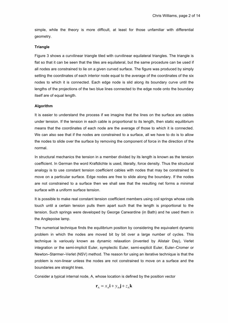
Consider a typical internal node, A, whose location is defined by the position vector
rA = xAi + yA j + zAk

Chris Williams, page 3 of 14
i , j and k are unit vectors in the directions of the Cartesian coordinate axes. If it is
surrounded by six nodes, B, C, D, E, F, and G, the net force from the six cables is
FA = !(rB " rA ) + !(rC " rA ) + !(rD " rA ) + !(rE " rA ) + !(rF " rA ) + !(rG " rA ) where ! is the constant tension coefficient. If a node is only connected to four nodes then
there would only be four contributions to the force.
If the nodes are constrained to move on a surface FA is replaced by
FA ! (FA • n)n
in which n is the unit normal to the surface at A and the • denotes the scalar product. This
removes the component of FA normal to the surface. It is easiest to specify the surface in the
form f (x, y, z) = 0 , because then the unit normal to the surface is
"x "y "z 2 2 2
"f "f j + "fi + k
!f • !f !fn = = .
# "f & # "f & # "f & $% "x ('
+ $% "y'(
+ $% "z '(
If a node is slightly off the surface it can be put back onto the surface by moving it by
# f &! $% "f • "f '(
"f .
In a time interval !t the velocity of node A changes from vA to
(1 ! ")vA + FA #t m
in which m is the real or fictitious mass of each node and ! is a factor to represent
damping. In the same time interval rA will change by vA!t .
All the forces on the nodes are calculated in each cycle before updating the velocities and
!"t 2
coordinates. The rate of convergence is controlled by the values of ! and , which are m
!"t 2
both dimensionless ratios. Typically ! = 0.01 to 0.001 gives the best results and is m
chosen by trial and error, if it is too low the procedure is slow, but if it is too large instability
will result.

Chris Williams, page 4 of 14
Icosahedron and sphere
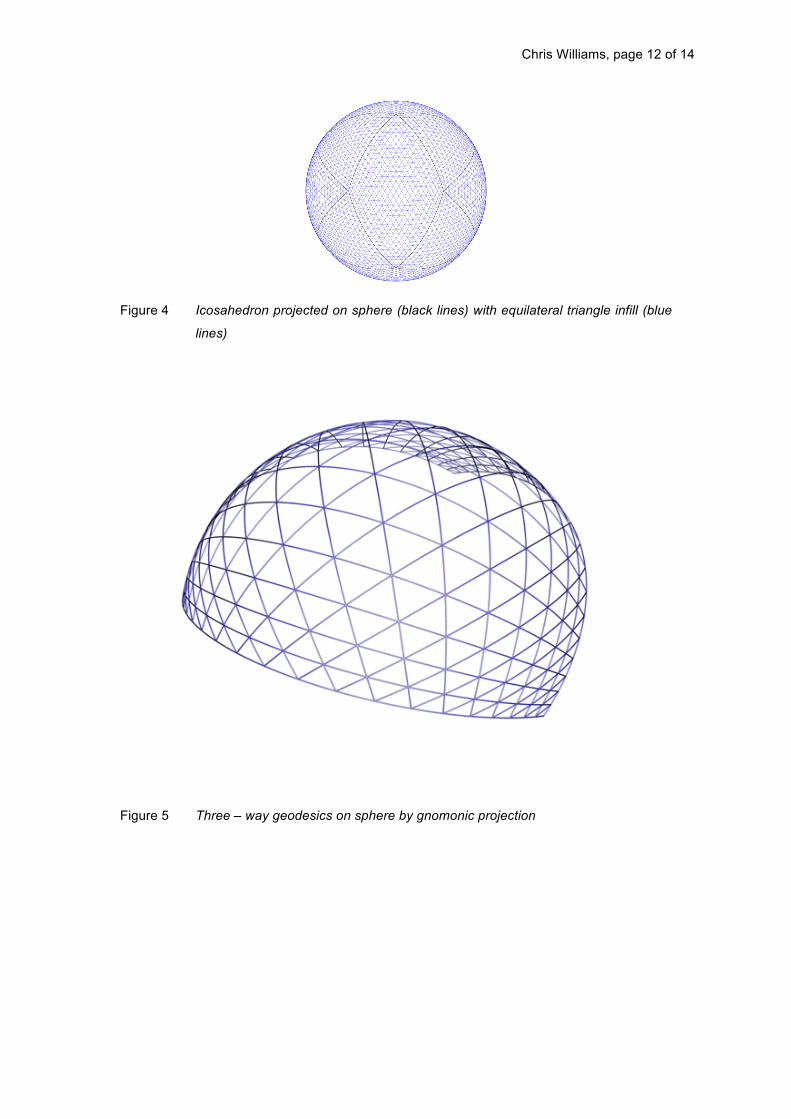
The black lines in figure 4 are the projection of the edges of an icosahedron onto a sphere.
The sphere and icosahedron share the same centre and the projection is done using straight
lines. If a plane is covered with a grid of straight lines, it can be projected onto the sphere to
form geodesics (figure 5), again using straight lines through the centre of the sphere. This is
known as gnomonic projection and it is almost certainly what Buckminster Fuller used for his
geodesic domes. However in figure 4 the blue lines form equilateral triangles and close
examination of the figure shows that the blue lines do have geodesic curvature, that is
curvature in the plane of the surface and are therefore not geodesics. It is not possible to
have both geodesics and equilateral triangles.
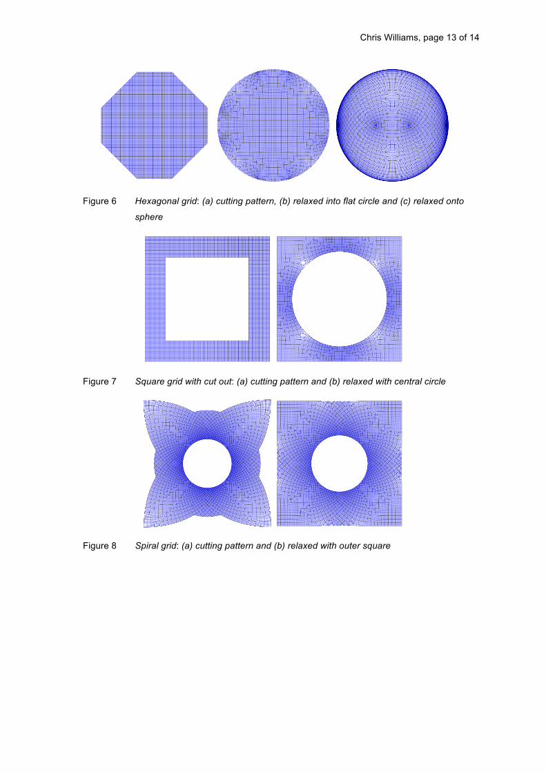
Hexagon and circle, hexagon and sphere
Figures 6 a, b and c show a hexagon relaxed onto a flat circle and onto a sphere. On the
sphere the grid is repeated twice, once for the top and once for the bottom, the upper and
lower parts of figure 6c. The half squares at the edges of figures 6a and 6b join to form full
squares on the sphere.
Circle and square
Figures 7 and 8 attempt the title of this paper, the reconciliation of the circle and the square.
There is a clear relationship between figure 8 and figure 2, the main difference being that in
figure 2 there is a third set of black lines dividing the quadrilaterals into triangles. The
triangles were chosen for the British Museum gridshell primarily for structural reasons. In the
numerical work to produce both figures 7b and 8b it was necessary to automatically adjust the
diameter of the circle to achieve curvilinear squares rather than curvilinear rectangles. The
reason for this is explained in the theoretical discussion.
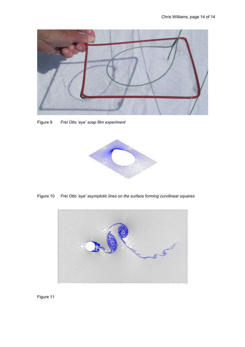
Frei Otto ‘eye’
Finally, figures 9 and 10 show the Frei Otto ‘eye’. Figure 9 is a physical experiment using
washing-up fluid. The trick is to keep the wool loop taut with your fingers while someone else
pops the soap film inside the loop. The wool then forms a circle which can be gently pulled
up. We will leave discussion of figure 10 for now, except to say that it was formed in the same
way as the other figures with the net automatically forming the minimal surface. Soap film
surfaces are minimal because the surface tension automatically reduces the surface area to a
minimum.
Theoretical discussion
Consider a surface defined by the three equations

Chris Williams, page 5 of 14
x = x u,v)( y = y u( ,v) or r = x u,v) i + y u,v) j + z u,v z = z u,v)
( ( ( )k
(
in which u and v are parameters or surface coordinates and r is a position vector.
However, we shall not use u and v as parameters, but instead use x1 and x2 which are
two separate parameters, NOT x to the power one and x squared. The reason for the
superscripts is that we can then use the tensor notation. Eisenhart [2] uses parameters u1
and u2 , whereas Green and Zerna [3] use !1 and ! 2 . Green and Zerna has the advantage
that it covers shell theory, that is the equilibrium of surfaces as well as their geometry. Struik
[4] uses u and v are parameters and the following table shows a comparison of the three
notations:
Quantity Struik Eisenhart Green and Zerna This paper
Surface parameters or
coordinates u and v u! where !
equals 1 or 2
!" where ! equals 1 or 2
xi where i equals 1 or 2
Covariant base vectors xu and xv - a! = r,! = "r "x! gi =
!r !xi
Contravariant base
vectors - - a! gi
Coefficients of the first
fundamental form,
components of metric
tensor
E , F and
G g!" a!" gij
Coefficients of the
second fundamental
form
e , f and g d!" b!" bij
Christoffel symbols -! "#
$&% '&
(&)*&
!"# $ ! ij
k
Covariant derivative of
the components of a
vector
- v j ,i v j |i !iv j

Chris Williams, page 6 of 14
Quantity Struik Eisenhart Green and Zerna This paper
Components of
membrane stress in a
shell
- - n!" ! ij
Two way net
In a two way net a typical node (i, j) , is connected to four neighbours, (i + 1, j) , (i, j + 1) , (i ! 1, j) and (i, j ! 1) . If the tension coefficient is taken as unity, the resulting out of balance
force on node (i, j) is the component of
(ri+1, j ! ri, j )+ (ri, j+1 ! ri, j )+ (ri!1, j ! ri, j )+ (ri, j!1 ! ri, j ) = (ri+1, j ! 2ri, j + ri!1, j )+ (ri, j+1 ! 2ri, j + ri, j!1 )
in the local tangent plane to the surface. The equivalent continuum quantity is the component
of
!!
x1
"#$ !!xr 1
% !!
x2
"#$ !!xr 2
%& (!
!
x
2
1
r
)2 + (!!
x
2
2
r
)2
!!gx11 +
!!gx22=' + ' =
&
in the local tangent plane. Thus for equilibrium,
" !g1 !g2 %' • g1 = 0#$ !x1
+ !x2 &
. " !g1 !g2 %' • g2 = 0#$ !x1
+ !x2 &
The components of the metric tensor, gij = gi • g j , and therefore
!gjk !g j • gk + g j • !gk=
!xi !xi !xi
!!gxki j
!!gx kj • gi + gk •
!!x gij =
!!gxij k !
!xgki • g j + gi •
!!g xkj=
!gi • gk = 1 # !gjk !gki !gij &"
!x j 2 $% !xi + !x j !xk '(
!gi !2r !g jsince !x j !xi!x j !xi
.= =
Thus the equilibrium equations become

1 2 2 2
121 2
122 2
Chris Williams, page 7 of 14
21 $%# !!gx11 k +
!!gxk11 !
!gx11 k '&( +
21 $%# !!gx22 k !
!gxk 22 !
!gx22 k '(& = 0" + "
for k = 1 and k = 2 . The metric tensor is symmetric ( gij = gji ) and so
!gk1 1 !g11 + !gk 2 1 !g22 = 0" "
!x1 2 !xk !x2 2 !xk
or
1 ! !g12 = 02 !x1 (g11 " g22 ) +
!x2
1 ! !g12 = 0 .
" 2 !x2 (g11 " g22 ) +
!x1
These are the Cauchy–Riemann equations and produce
!2 !2
(!x ) (g11 " g22 )+ (!x ) (g11 " g22 ) = 0
!2g !2g .
+ = 0(!x ) (!x )
Thus both (g11 ! g22 ) and g12 satisfy Laplace’s equation. Note that here we have just partial
derivatives, NOT covariant derivatives which one would normally associate with differential
equations on a surface.
Examination of figures 7a and 7b shows that the sliding boundary condition means that the
cables are orthogonal on all boundaries, except at the singular points corresponding to the
corners of the inner square. Adjustment of the circle radius removes this problem to produce
g12 = 0 on all boundaries, and therefore Laplace’s equation tells us that g12 = 0
everywhere. Thus !!
x1 (g11 " g22 ) = 0 and !!
x2 (g11 " g22 ) = 0 so that
g11 ! g22 = constant everywhere. Thus we must have curvilinear rectangles, all with the
same difference in the square of the side lengths. In the case of figure 7b symmetry tells us
that the rectangles must be squares – provided that we have the correct circle radius to
ensure g12 = 0 .
The sphere in figure 6c has no boundaries, although it does have eight poles, whereas the
sphere in figure 4 has twelve poles. In figure 8b the boundary conditions are mixed. On the
circle and towards the middle of each side g11 ! g22 = 0 , whereas towards the ends of each
side g12 = 0 . Again it was necessary to adjust the circle diameter to achieve curvilinear
squares.
Chris Williams, page 8 of 14
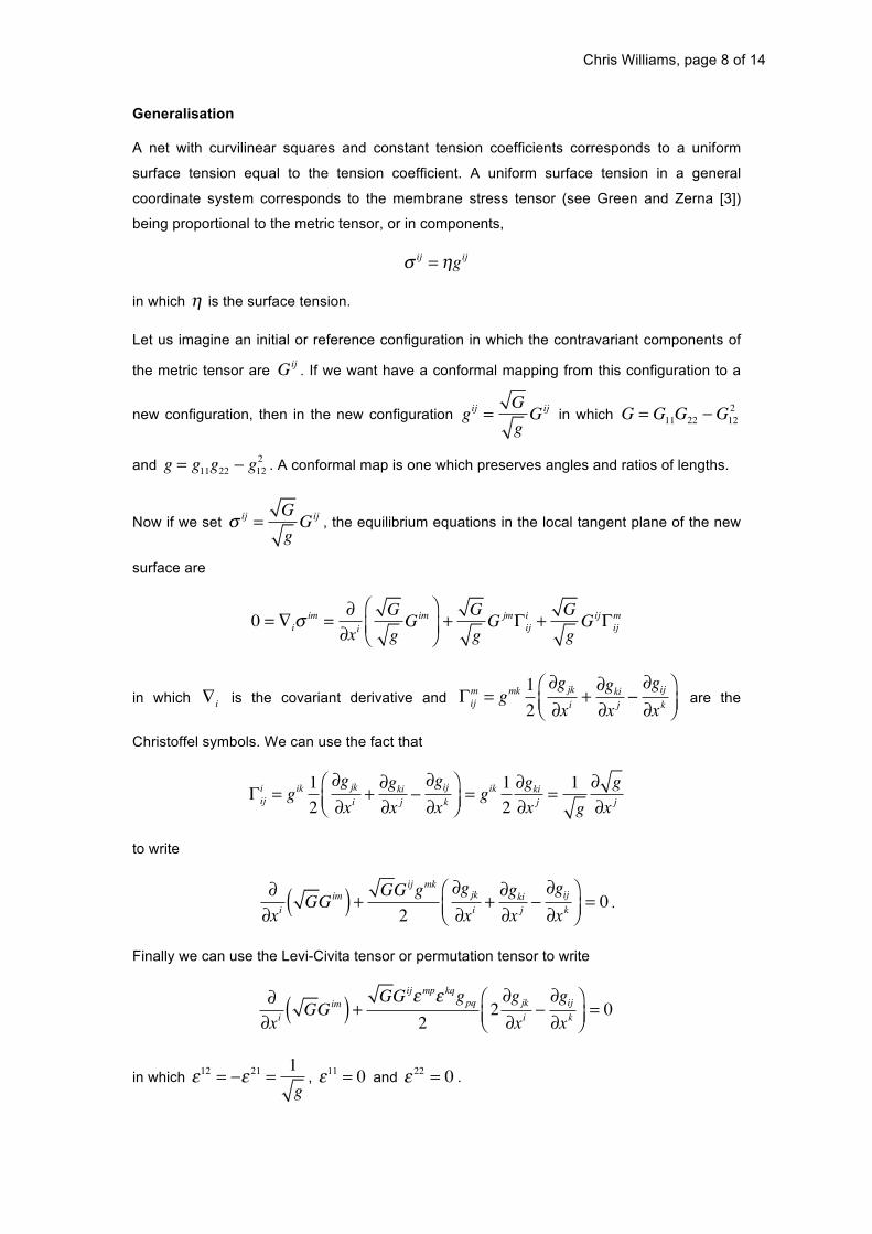
Generalisation
A net with curvilinear squares and constant tension coefficients corresponds to a uniform
surface tension equal to the tension coefficient. A uniform surface tension in a general
coordinate system corresponds to the membrane stress tensor (see Green and Zerna [3])
being proportional to the metric tensor, or in components,
! ij = "gij
in which ! is the surface tension.
Let us imagine an initial or reference configuration in which the contravariant components of
the metric tensor are Gij . If we want have a conformal mapping from this configuration to a
Gij 2new configuration, then in the new configuration gij = in which G = G11G22 ! G12
Gg
and g = g11g22 ! g12 2 . A conformal map is one which preserves angles and ratios of lengths.
Now if we set ! ij = Gij , the equilibrium equations in the local tangent plane of the new Gg
surface are
' Gim m0 = !i " im
##
xi $
%& Gg ()
+ Gg G jm* ij
i + Gg Gij * ij =
+in which is the covariant derivative and are the !i ! ij m = gmk
12
$%& ""gxjk i
""gxki j #
""gxij k
'()
Christoffel symbols. We can use the fact that
=! ij i = gik
21
%&$ ""gxjk i +
""gxki j #
""gxij k ()' = gik
21 ""gxki j
g
"x j 1
g
"
to write
GGij gmk
2
# !gjk + !gki !gij & = 0 .
!!
xi ( GGim ) + "
$% !xi !x j !xk '(
Finally we can use the Levi-Civita tensor or permutation tensor to write
GGij" mp" kq gpq $ 2 !gjk !gij '
2 %& !xi #!xk ()
= 0!
!xi GGim ( ) +
in which !12 = "! 21 = 1
, !11 = 0 and ! 22 = 0 . g

Chris Williams, page 9 of 14
If we return to the special case of the curvilinear squares, then G11 = 1 , G22 = 1 , G12 = 0
and G = 1, so that
2 !g1k !g11 + 2
!g2k !g22 = 0" " !x1 !xk !x2 !xk
which produces
1 ! (g11 " g22 ) + !g12 = 0
2 !x1 !x2
" 1
!!
x2 (g11 " g22 ) + !!gx121 = 0
2
as above.
Equilateral triangular nets
If we have a uniform equilateral triangular net in the initial configuration, then G11 = 1 ,
G22 = 1 , G12 = ! 1
= !2 and G = 1
= 43
so that cos60º 1 ! cos2 60º
2 !g1k !g11 + 2
!g2k !g22 #" " " 2 2 !g2k "
!g12 + 2 !g1k !g21 &"
!x1 !xk !x2 !xk $% !x1 !xk !x2 !xk '( = 0
or
! ) = 4 !g11 " 2
!g12
!x1 (g11 " g22 !x2 !x2
.
"! ) = 4
!g22 " 2 !g12
!x2 (g11 " g22 !x1 !x1
These are satisfied by g11 = g22 = 2g12 which is the requirement for a curvilinear equilateral
triangle net.
Minimal surfaces
A minimal surface is a surface of minimum surface area which can be physically modelled by
a soap film. Minimal surfaces have many interesting properties, amongst whish is the fact that
the principal curvature trajectories form curvilinear squares on the surface. On a minimal
surface the asymptotic directions (which are the directions of zero normal curvature) are at
45º to the principal curvature directions and therefore their trajectories also form curvilinear
squares on the surface.
If a soap film has a boundary which is a thread under tension, then equilibrium of the thread
dictates that the curvature of the thread must be constant and lie in the local tangent plane to
the soap film surface. This means that the boundary must be an asymptotic trajectory. And
these facts were used to produce the minimal surface in figure 10. The nodes are free to

Chris Williams, page 10 of 14
move in the direction normal to the surface, automatically producing a minimal surface. The
main problem is the adjustment of the thread length and the cutting pattern in order to
produce curvilinear squares. Included in this adjustment is the fact that the maximum slope
along the straight edges must occur at a point where the curvilinear squares are theoretically
infinitely large.
Conclusions
The technique provides a relatively simple method of tiling a surface with curvilinear tiles of
constant shape, but varying size. In the case of a triangular region equilateral triangles can
always be used, but for other shapes care must be taken with the boundary conditions to
ensure that the tiles are of the same shape. For minimal surfaces, the technique can both find
the shape and produce a principal curvature or, alternatively, an asymptotic direction net.
In this paper we have used the Laplace’s equation, or the harmonic equation, associated with
the operator !2 . This means that we have one boundary condition. The biharmonic equation,
associated with !4 , allows two boundary conditions, for example the position and slope of a
bent elastic plate. The flow of fluids in two dimensions can be modelled using an analogy of a
bent plate in which mean curvature of the plate is equal to the fluid vorticity. Figure 11 was
produced this way using techniques not that dissimilar to those employed in this paper. The
black streamlines are the contours of height of the plate and the blue streak shows the
starting of vortex shedding. The reason for including this figure is to demonstrate the
complexity of patterns that develop in nature, again effectively from the interaction of
rectangular and circular geometries.
References
1. Chris J K Williams, C.J.K. ‘The definition of curved geometry for widespan structures’,
41-49, Widespan roof structures, Barnes, M. and Dickson, M. eds. Thomas Telford,
London, 2000, ISBN 0 7277 2877 6.
2. Luther Pfahler Eisenhart, An Introduction to Differential Geometry with Use of the
Tensor Calculus, Princeton University Press, 1940.
3. A E Green and W Zerna, Theoretical Elasticity, 2nd Edition, Oxford University Press,
1968.
4. Dirk J. Struik, Lectures on Classical Differential Geometry, 2nd Edition, Dover
Publications, 1988.

Chris Williams, page 11 of 14
Figures
Figure 1 The British Museum Great Court Roof by Foster + Partners, Buro Happold and
Waagner-Biro
Figure 2 Great Court Roof structural and ‘mathematical’ grids
Figure 3 Curvilinear triangle tiled with curvilinear equilateral triangles
Chris Williams, page 12 of 14
Figure 4 Icosahedron projected on sphere (black lines) with equilateral triangle infill (blue
lines)
Figure 5 Three – way geodesics on sphere by gnomonic projection
Chris Williams, page 13 of 14
Figure 6 Hexagonal grid: (a) cutting pattern, (b) relaxed into flat circle and (c) relaxed onto
sphere
Figure 7 Square grid with cut out: (a) cutting pattern and (b) relaxed with central circle
Figure 8 Spiral grid: (a) cutting pattern and (b) relaxed with outer square
Chris Williams, page 14 of 14
Figure 9 Frei Otto ‘eye’ soap film experiment
Figure 10 Frei Otto ‘eye’ asymptotic lines on the surface forming curvilinear squares
Figure 11
Related Documents