Optimizing the regularization for image reconstruction of cerebral diffuse optical tomography

Optimizing the regularization forimage reconstruction of cerebraldiffuse optical tomography

Christina HabermehlJens SteinbrinkKlaus-Robert MüllerStefan Haufe

Downloaded From: http://biomedicaloptics.spiedigitallibrary.org/ on 10/13/2014 Terms of Use: http://spiedl.org/terms

Optimizing the regularization for image reconstructionof cerebral diffuse optical tomography

Christina Habermehl,a,b,c,* Jens Steinbrink,b,d Klaus-Robert Müller,a,b,e,f and Stefan Haufea,b

aBerlin Institute of Technology, Department of Computer Science, Machine Learning Group, Marchstraße 23, Berlin 10587, GermanybBernstein Focus Neurotechnology, Department of Computer Science, Marchstraße 23, Berlin 10587, GermanycCharité University Medicine, Department of Neurology, Charitéplatz 1, Berlin 10117, GermanydCharité University Medicine, Center for Stroke Research, Charitéplatz 1, Berlin 10117, GermanyeBernstein Center for Computational Neuroscience, Humboldt-Universität zu Berlin Philippstr. 13, Berlin 10115, GermanyfKorea University, Department of Brain and Cognitive Engineering, Anam-dong, Seongbuk-gu, Seoul 136-713, Republic of Korea

Abstract. Functional near-infrared spectroscopy (fNIRS) is an optical method for noninvasively determiningbrain activation by estimating changes in the absorption of near-infrared light. Diffuse optical tomography(DOT) extends fNIRS by applying overlapping “high density” measurements, and thus providing a three-dimen-sional imaging with an improved spatial resolution. Reconstructing brain activation images with DOT requiressolving an underdetermined inverse problem with far more unknowns in the volume than in the surface mea-surements. All methods of solving this type of inverse problem rely on regularization and the choice of corre-sponding regularization or convergence criteria. While several regularization methods are available, it is unclearhow well suited they are for cerebral functional DOT in a semi-infinite geometry. Furthermore, the regularizationparameter is often chosen without an independent evaluation, and it may be tempting to choose the solution thatmatches a hypothesis and rejects the other. In this simulation study, we start out by demonstrating how thequality of cerebral DOT reconstructions is altered with the choice of the regularization parameter for differentmethods. To independently select the regularization parameter, we propose a cross-validation procedure whichachieves a reconstruction quality close to the optimum. Additionally, we compare the outcome of seven differentimage reconstruction methods for cerebral functional DOT. The methods selected include reconstruction pro-cedures that are already widely used for cerebral DOT [minimum l2-norm estimate (l2MNE) and truncated sin-gular value decomposition], recently proposed sparse reconstruction algorithms [minimum l1- and a smoothminimum l0-norm estimate (l1MNE, l0MNE, respectively)] and a depth- and noise-weighted minimum norm(wMNE). Furthermore, we expand the range of algorithms for DOT by adapting two EEG-source localizationalgorithms [sparse basis field expansions and linearly constrained minimum variance (LCMV) beamforming].Independent of the applied noise level, we find that the LCMV beamformer is best for single spot activationswith perfect location and focality of the results, whereas the minimum l1-norm estimate succeeds with multipletargets. © The Authors. Published by SPIE under a Creative Commons Attribution 3.0 Unported License. Distribution or reproduction of this work in

whole or in part requires full attribution of the original publication, including its DOI. [DOI: 10.1117/1.JBO.19.9.096006]

Keywords: diffuse optical tomography; near-infrared spectroscopy; brain imaging, simulation; image reconstruction; inverse problem.

Paper 140276R received Apr. 30, 2014; revised manuscript received Jul. 23, 2014; accepted for publication Jul. 24, 2014; publishedonline Sep. 10, 2014.

1 IntroductionDiffuse optical tomography (DOT) is a modality of near-infraredspectroscopy (fNIRS) that provides three-dimensional (3-D)images of absorption changes in a semi-infinite volume.Recently, it has been applied in breast cancer imaging or opticalmammography1–3 as well as in small animal imaging.4–6 The3-D DOT has been proposed by various groups7–14 for imagingbrain function.

Used as a brain-imaging tool, DOT measures the changes innear-infrared light absorption in the cortex. It allows the operatorto determine what functional changes are evoked in cerebraloxygenated (HbO2) and deoxygenated hemoglobin (HbR) con-centration in the cerebral blood flow during local brain activa-tion. Due to the wavelength-dependent light attenuation, DOTusually employs two different wavelengths, each of them moresensitive to one of the main chromophores HbO2 and HbR.

Compared to fNIRS, DOT uses more light sources and detectorsin a high-dense optical fiber grid, and allows many overlappingoptical data channels with different source-detector distancesto be recorded. Light, which is detected far away from thesource, passes through the deeper tissue layers, allowing the sep-aration of superficial layers from cerebral layers in a 3-Dmanner.15,16

Recovering the absorption coefficient μa inside the headfrom boundary measurements is a nonlinear problem, but itcan be linearized if scattering (μs) in the head is stable overtime and the change in μa is small (perturbation approach).For image recovery, light propagation in the examined tissueneeds to be modeled first. In tissue, where scattering dominatesabsorption and the propagation of light is close to isotropic, thediffusion equation can be applied for modeling. After discreti-zation of the scanned volume (e.g., as a finite-element (FE)mesh), wavelength-specific optical properties are assigned tothe elements (mesh nodes), and light propagation is modeledwith respect to the positions of the optical fibers on the surface.Solving the forward problem results in a weight matrix J that

*Address all correspondence to: Christina Habermehl, E-mail: [email protected]

Journal of Biomedical Optics 096006-1 September 2014 • Vol. 19(9)

Journal of Biomedical Optics 19(9), 096006 (September 2014)


http://dx.doi.org/10.1117/1.JBO.19.9.096006






mailto:[email protected]



contains sensitivity values for all nodes in the reconstructionvolume for all given light source and detector pairs.

Reconstruction of DOT images requires inverting the for-ward mapping J. This is an under-determined and ill-posedproblem, since countless distributions of μa within the volumecan explain the same surface measurement. Moreover, near-infrared light can pass skin and bone, but is highly attenuatedwith increasing depth, causing J to be ill conditioned (or evensingular), and the solution to the corresponding linear system tobe prone to numerical instabilities. With a penetration depth of3 to 4 cm, light can reach the cortex, but there is a vast sensi-tivity loss in the depth. This leads to a sparse matrix with verylow sensitivity values in the largest fraction of the volume.Furthermore, small changes in optical properties at this depthhave to be recovered from boundary measurements with nearbynodes that have a high sensitivity to superficial signals and are,therefore, sensitive to noise. Due to the ill-posed nature of theDOT inverse problem, a unique solution can only be obtained ifthe constraints are imposed on the distribution of the absorptioncoefficients. Moreover, since J is ill-conditioned, a solution hasto be found that optimally suppresses noise while still explainingthe data. Many studies using DOT either add an additionalregularization term to the model or eliminate the singular valuessmaller than a defined threshold from J. Both methods over-come the problem of very small singular values of J causingamplification of noise upon inversion. However, the choiceof a regularization parameter (either the number of singular val-ues maintained or the relative weight of the regularization termin the cost function) is often made ad hoc8,17–19 and lacks objec-tive criteria. For researchers, it may be challenging to find anappropriate regularization parameter, since the measured datavary highly between the experiments, depending on the setup,imaging device, tissue properties, and noise level.

Besides the problem of regularization, the distributed sourcelocalization methods such as minimum l2-norm estimate(l2MNE) and truncated singular value decomposition (tSVD)tend to yield blurry images rather than focused results.Therefore, a variety of sparse image reconstruction methods,such as lp-norm-based algorithms with 0 ≤ p ≤ 1, have beenintroduced in optical imaging.20–24

Other approaches to reconstruct the brain activation are pro-vided by developments in electrophysiological dipole mapping.The inverse problem of electroencephalography (EEG) localizesthe position of the active cerebral current source from the mea-sured surface fields, and is comparable with the inverse problemof image reconstruction in DOT.

The aim of this work is twofold. First, we show how thereconstruction quality in cerebral DOT depends on the amountof regularization chosen when distributed source localizationmethods (e.g., minimum norm estimates and tSVD) are used.We demonstrate the need for an independent parameter selectionbased on the features of the measurement data. To this end,we propose cross-validation (CV) for parameter selection. Thisyields high quality results and allows for an automatic data-driven determination.

Second, we benchmark the outcome of seven imagereconstruction methods which are:

• widely applied standard reconstruction methods such astSVD, l2MNE, and a depth- and noise-weighted variant;

• recently proposed sparse methods (minimum l1- anda smooth minimum l0-norm estimate), 17,21–24

• and finally, two EEG source localization algorithmsadapted to DOT. More precisely, we apply the linearlyconstrained minimum variance (LCMV) beamformer25

and a method for source localization using spatial flexi-bility (S-FLEX). S-FLEX has proven to be a good com-promise between focality and smoothness, and allows therecovery of multiple activation foci from EEG data.26

Our simulation mimics a cerebral DOT experiment. It pro-vides a very realistic framework using an atlas-based five-lay-ered head model in combination with real-world noise data,which are added to the simulated signals to take fiber dis-tance-dependent noise levels. Rather than using transilluminatedcylindrical (or breast tissue mimicking) geometries with onereconstructed sample point (e.g., to detect areas with differentoptical properties, such as tumors), we performed this studyon a semi-infinite medium with a highly attenuated light sensi-tivity in deeper layers. Additionally, an enormous amount ofdata is being processed, as is typical for high-density cerebralDOT since it is used to record thousands of sample points inhundreds of optical data channels.

2 Methods

2.1 Head Atlas and Meshing

To achieve a simulation setting which is close to a real meas-urement, we used the Montreal ICBM 2009a atlas, an unbiasednonlinear average of 152 anatomical MR images with 1 mm3

voxel size,27,28 and corresponding tissue probability maps forcerebrospinal fluid, gray matter, and white matter.29 In order toobtain a five-compartment model including scalp and skull, weadditionally segmented the ICBM2009a images using math-ematical morphological operations.30 Based on this segmentedbrain atlas [see Fig. 1(a)], we used a masking and meshing soft-ware (Nirview)31 to create a 3-D tetrahedral mesh [Fig. 1(c)].This mesh was used to calculate the photon transport, andthus provides the framework to simulate the cortical activationand to test the outcome of different reconstruction methods.

2.2 Forward Simulation and Spatial Constraints

Optical fiber positions on the boundary of the FE mesh werechosen according to the setting of a previous real-world cerebralDOT experiment conducted under resting conditions [Fig. 1(b)].Due to the use of registration landmarks from the EEG 10–20reference system32 and known source-detector distances, thecoordinates for each fiber were known. To model light propa-gation, we used the Nirfast software toolbox,33 a MATLAB®-based publicly available light modeling and reconstructionsoftware. Nirfast applies the diffusion equation approximation,which is appropriate when scattering events dominate overabsorption and the medium can be assumed to be an isotropicfluence field.

One challenge in DOT is the sensitivity of the measurementto signals coming from noncortical regions. The HbO2 specificwavelength is often contaminated with hemodynamic fluctua-tions from superficial veins in the scalp.34 On the other hand,the decrease in absorption from the HbR sensitive wavelengthis highly correlated to the BOLD response in functional mag-netic resonance imaging.35 For this simulation study, we uselight model and data from the HbR sensitive wavelength of760 nm. Optical properties μa and μ 0

s were assigned to eachnode of the FE mesh according to Strangman et al.36


Habermehl et al.: Optimizing the regularization for image reconstruction. . .


The result of the simulated light propagation is a sensitivity/Jacobian matrix J with dimensionsM × N, whereM is the num-ber of measurements (optical data channels) and N is the num-ber of nodes in the reconstruction volume. J describes thelogarithmic relationship between changes in measured boundarydata (Δy) that are caused by small changes of μa within the tis-sue for each channel-node combination, where

Δy ¼ JΔμa: (1)

Since the reconstruction volume was not entirely coveredwith the optode set, and since DOT has only a limited penetra-tion depth of 3 to 4 cm, we constrained J in order to reduce theresult space and thus reduce the “degree of ill-posedness.” Onecriterion for the exclusion of nodes was their affiliation to thenoncortical tissue. Nodes belonging to scalp, skull, or cerebro-spinal fluid were discarded. To exclude “weak” channels withvery low sensitivity (e.g., due to large source-detector separa-tion), we calculated the vector norm for all rows of J. Rowshaving a norm lower than 1% of the maximum value werediscarded. The same procedure was performed for the meshnodes, excluding nodes from the result space that had hardlybeen reached by any measuring channel. This step reducedthe result space from 256 to 232 channels, and from 150,000to 10,000 nodes. In the following, we refer to this reducedJacobian as J with the dimension of M measuring channelsand N reconstruction nodes. Figure 1(d) depicts the total sensi-tivity of J and Fig. 1(e) depicts J, which is calculated as the sum

of the sensitivity over all measurement pairs for all used nodeswithin the head volume.

2.3 Signal Generation and Noise Model

As an input signal, we modeled a hemodynamic response func-tion (hrf) for absorption changes at 760 nm peaking 5 s afterstimulus onset,37 thereby mimicking a 400 s experiment witha stimulus duration of 20 s and an interstimulus interval of20 s. This was necessary for testing the LCMV beamformerreconstruction method, which requires time-series data.Moreover, it allowed us to superimpose the artificial datawith realistic noise of the same dimensionality obtained fromthe abovementioned resting-state recording.

Detector readings were generated as follows. A sparse matrixAsim with the dimension of N × Nactive was created, where Nc isthe number of “activated” nodes. Each column of Asim labels onenode by setting AsimðlÞ ¼ 1 at a specific location l, while allother nodes are set to “0.” The locations for these “activated”nodes were randomly chosen, but due to restrictions of thereduced Jacobian J, all nodes were cortical. The specific sensi-tivity pattern p in the activated node/nodes is defined by

p ¼ J � Asim; (2)

with p having the dimensions M × Nactive, and the simulatedDOT measurement y defined by the M × sampleshrf matrix

y ¼ p � hrf; (3)

Fig. 1 (a) Segmented head atlas (ICBM 2009a, a nonlinear average of 152 MR images). From outer toinner layers: scalp, skull, cerebrospinal fluid, gray matter, white matter, (b) sketch of the optical fiber setupas used in the forward model (first nearest neighbor distance: 13 mm, (c) finite-element (FE) mesh ofthe left hemisphere with optical properties (μa), (d) example of the total sensitivity of determined fromthe unconstrained Jacobian J . A cross section of the sensitivity volume is superimposed on the corre-sponding layer of the head model, (e) total sensitivity of the spatially constrained Jacobian ~J : sensitivitiesfor skull, scalp and CSF were set to zero.




where the Nactive × sampleshrf matrix hrf contains the activationsof the simulated brain activity at the active nodes.

We applied a realistic noise model for the purpose of testingdifferent reconstruction algorithms under natural conditions.Most studies added white noise to the data to simulate thereal measurements. In real life measurements, however, thenoise is usually temporally and spatially correlated and is notnormally distributed. We typically observe a higher increasednoise level for larger source-detector separations than that forshort distances. Second, the noise often has a high fractionof hemodynamic oscillations, which may interfere with thehemodynamic response and are sometimes hard to remove.Rather than applying a random noise term, we utilized datafrom a 10-min DOT experiment conducted under resting condi-tions as the noise model ℵ. For recording these resting-statedata, we used a compact tomography imager that provides upto 32 sources × 32 detectors (NIRScoutX Tomography Imager,NIRx Medizintechnik, Berlin, Germany). This allowed us toachieve realistic simulation data with characteristic featuresof the real measurements. The setup for that resting-state experi-ment was the same as that of the simulation setup, so that fiberdistances and orientations were preserved.

We selected the rows of the noise matrix ℵ according tothe choice of channels for J, so that identical channels wereused. Additionally, we took a subset of sampling/time points(columns) from ℵ, so that y and ℵ had the same dimensions.

Finally, ℵ and y were normalized by their respectiveFrobenius norms in order to calibrate the artificial measurementand noise matrix. Given y, ℵ and s, where s is the signal levelwith a value between 0 and 1, the noisy simulated measurementyℵ was constructed as

yℵ ¼ ysþ ℵð1 − sÞ: (4)

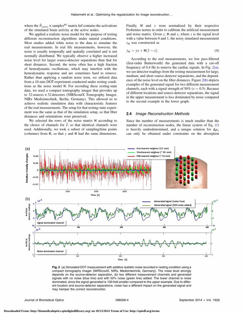
According to the real measurements, we low pass-filtered(first-order Butterworth) the generated data with a cut-offfrequency of 0.4 Hz to remove the cardiac signals. In Fig. 2(a),we see detector readings from the resting measurement for large,medium, and short source-detector separations, and the depend-ence of the noise level on the fiber distances. Figure 2(b) depictsexamples of the generated signal for two different measurementchannels, each with a signal strength of 50% (s ¼ 0.5). Becauseof different locations and source-detector separations, the signalin the upper measurement is less dominated by noise comparedto the second example in the lower graph.

2.4 Image Reconstruction Methods

Since the number of measurements is much smaller than thenumber of reconstruction nodes, the linear system of Eq. (1)is heavily underdetermined, and a unique solution for Δμacan only be obtained under constraints on the absorption

Fig. 2 (a) Simulated DOTmeasurement with additive realistic noise recorded in resting condition using acompact tomography imager (NIRScoutX, NIRx, Medizintechnik, Germany). The noise level stronglydepends on the source-detector separation, (b) two different measurement channels and generatedsignals with no noise (blue line) and with 50% noise (green line) added. The lower channel is noisedominated, since the signal generated is 100-fold smaller compared to the upper example. Due to differ-ent location and source-detector separations, noise has a different impact on the generated signal andmay hamper the correct reconstruction.




coefficient distribution. In order to find a solution which isneuro-physiologically plausible, these constraints should alwaysencode valid prior assumptions on the properties of Δμa.Various such assumptions have been proposed in the literatureon an EEG/MEG inverse problem, which has a similar math-ematical structure. In the following paragraphs, we introducethe approaches tested. As in previous parts of the paper, weomit the dependence of Δμa and Δy on time. Thus, unless statedotherwise, a separate reconstruction is performed for each timepoint (i.e., difference measurement).

2.4.1 Minimum l2-norm estimate

A common way of constraining the brain source activity Δμa isto penalize its norm, thereby encoding a preference for the“least-active” (or, “least-complex”) brain state that gives riseto the measurement. In the simplest case, the complexity ismeasured using the l2 norm. The minimum l2 norm estimate(l2MNE) of the DOT inverse problem can be written as

Δμa ¼ argminΔμa

kJΔμa − Δyℵk22 þ λkΔμak22; (5)

where λ adjusts the degree of regularization.38 The solution isobtained as

Δμa ¼ HλΔyℵ; (6)

where

Hλ ¼ JTðJJT þ λIÞ−1 (7)

is a precomputable pseudoinverse matrix and I is the M × Midentity matrix.

2.4.2 Minimum l1-norm estimate

In the EEG/MEG literature, it is often noted that linear inverses(i.e., those employing l2-norm penalties) lead to blurred imagesof source activity, and are unable to simultaneously spatiallyseparate the multiple active brain sites.26,39 As a remedy, estima-tion of the brain activation maps using l1-norm penalties isoften suggested. Using l1-norm penalties leads to sparse solu-tions, i.e., activity maps, which are zero almost everywhere.Here, we consider a depth-weighted variant of the method pro-posed by Matsuura and Okabe.40 The minimum l1-norm solu-tion is given by


kJΔμa − Δyℵk22 þ λkWΔμak1: (8)

The weight matrixW is chosen to be the same as in Eq. (14).The minimum of Eq. (8) is obtained using an iterative optimi-zation algorithm.

2.4.3 Smoothed minimum l0-norm estimate

The method described in Ref. 41 has been applied to the cylin-drical geometry for DOT in Ref. 21. It aims at a direct minimi-zation of the l0-norm


kJΔμa − Δyℵk22 þ λkΔμak0: (9)

Thus, it searches for the solution with the smallest number ofactive voxels. Since this leads to a combinatorial optimization

problem, a smooth approximation of the (discontinuous) l0-norm of a vector is considered, which leads to optimizing asequence of certain continuous cost functions. The function,which approximates l0-norm, includes an additional parameterσ, which determines the quality of the approximation in terms ofbalancing smoothness and sparsity of the result.

2.4.4 Truncated singular value decomposition

The MNE solution Eq. (6) is defined for any positive regulari-zation constant λ. The limit

Jþ ¼ limλ→0

JTðJJT þ λIÞ−1 (10)

is called the Moore–Penrose (MP) pseudoinverse of J. The MPsolution JþΔyℵ is the source activity with the smallest l2-normthat exactly fulfills Eq. (1), whereas solutions HλΔyℵ for λ > 0no longer perfectly explain the data. The computation of Jþ canbe performed using the singular value decomposition (SVD)

J ¼ UΣVT (11)

of J, where Σ ¼ diagðσ1; : : : ; σMÞ is a M × M diagonal matrix,σ1 ≥ : : : ≥ σM are the singular values, U is an orthogonal ~M ×~M matrix with UTU ¼ UUT ¼ I, and V is an N × M matrixwith VTV ¼ I.

The MP pseudoinverse of J Eq. (10) can be equivalentlywritten as

Jþ ¼ VΣ−1UT: (12)

Similarly, for λ > 0, the SVD can be used to computeHλ ¼ VðΣþ λIÞ−1UT , and thus to solve Eq. (7). The formu-lation of Jþ in terms ofU, Σ, and V offers an alternative to regu-larizing the source activity using an l2-norm penalty. Given thatΣ−1 ¼ diagðσ−11 ; : : : ; σ−1

MÞ, it is possible to compute a reduced-

rank pseudoinverse

Jþm ¼ VmΣ−1m UT

m (13)

using truncated matrices Vm, Σ−1m , and Um, where the N ×m

matrix Vm and the M ×m matrix Um are obtained by selectingthe first m rows of V and U, respectively, and whereΣ−1m ¼ diagðσ−11 ; : : : ; σ−1m Þ is m ×m.Performing image reconstruction using ~Jþm corresponds to

constraining the source estimate JþmΔyℵ to lie within them-dimensional subspace of the brain, in which brain activitycontributes most strongly to the sensors.

2.4.5 Weighted minimum norm estimate

Reconstructing activations only in those parts of the brainhaving a high impact on the measurements (as in tSVD) is rea-sonable, since doing so ensures that weak signal components(which might simply be noise) are not overinterpreted.However, one often wants to ensure that activations fromdifferent parts of the brain are equally likely to be detected.To this end, weighted minimum-norm estimates (wMNE) areemployed. The idea here is to adjust the l2-norm penalty inEq. (5) to compensate for the different gains activation focihave at the detector level depending on their depth. Formally,this is achieved by introducing a ~N × ~N weight matrix W inthe penalty term:





kJΔμa − Δyℵk22 þ λkWΔμak22: (14)

The solution of Eq. (14) is given by

Δμa ¼ JTðJJT þ λWWTÞ−1Δyℵ: (15)

Here, we use a diagonal matrix W ¼ diagðw1; : : : ; wMÞand the entries wi ¼ Sii of which are the diagonals ofS ¼ JTðJJTÞ−1J.39

2.4.6 Sparse basis field expansions

The selection of active voxels by sparse inverses tends to beunstable and highly noise dependent.

Moreover, the l1 -norm penalty prevents multiple voxelswith correlated activity to be jointly selected, which maylead to scattered solutions. To cope with these shortcomings,it has been suggested to replace sparsity in voxel domain bysparsity in a space of appropriately defined spatial basis func-tions.26 The basis function dictionary of the proposed S-FLEX(sparse basis field expansion) approach consists of Gaussianblobs of different widths centered at each voxel. Sparsifyingthe expansion coefficients corresponding to these blobs amountsto integrating the assumption that “plausible” activation mapsare composed of a small number of blob-like activities, i.e.,have a simple structure.

Denoting the N × KN matrix of Gaussian basis functions byG and the vector of corresponding expansion coefficients by c,where K is the number of blob widths, S-FLEX decomposes theestimated brain source activity into

Δμa ¼ W−1Gc; (16)

where W is the weight matrix defined in the section above.S-FLEX minimizes the squared deviation from the data underan additional l1 -norm constraint ensuring the sparsity of c:

c ¼ argminc

kJW−1Gc − Δyℵk22 þ λkck1: (17)

The minimum of Eq. (17) is inserted into Eq. (16) to yield theestimated brain activationΔμa. Note that forG ¼ I, the S-FLEXsolution coincides with the weighted minimum l1-norm solu-tion Eq. (8).

For a time series, S-FLEX jointly estimates the brain activa-tions at all available time points under the assumption thata common set of spatial basis functions is active throughoutthe recording. To this end, coefficients corresponding to thesame basis function but different time instants are groupedtogether and are jointly sparsified using a so-called l1;2-normpenalty.26

Note that without this technique, the sparsity pattern wouldjump from each reconstructed sample to the next, entirely obfus-cating the temporal structure of the activations at the voxel level.We also use the technique of the minimum l1-norm approach.However, the minimum l0-norm approach, for which thisproblem also occurs, can not be extended to time-series dataas easily.

2.4.7 Linearly constrained minimum variance beamformer

In contrast to the previously discussed techniques, beamformingis not only concerned with estimating activity across the entire

brain at once, but a rather does the estimation separately for eachnode. To this end, the activity from each voxel q is extracted bymeans of a designated linear spatial filter vq, which is optimizedfor the given data Δyℵ. The estimated brain activity is obtainedas Δμa ¼ ½v1; : : : ; vN �TΔyℵ.

The idea of the LCMV beamformer is to construct filterswhich let signals from a specific location pass with unit gainwhile suppressing all noise components.25 The optimal filterfor location q is obtained as the solution to the optimizationproblem

vq ¼ argminvq

vTqCvq such that vTq Jq ¼ 1; (18)

where C is the covariance matrix of the data Δyℵ taken acrosstime, and ~Jq is the gain vector for the q-th voxel (the q-th col-umn of ~J). The solution is obtained as

vq ¼ ½JTqC−1Jq�−1JTqC−1: (19)

The linear constraint vTq ~Jq ¼ 1 ensures that brain activityfrom voxel q (i.e., the signal of interest) is not damped, whereasthe minimization of vTqCvq amounts to minimizing the overall(signal + noise) power of the projected data vqΔyℵ. In total,Eq. (19) maximizes the signal-to-noise ratio. However, thisonly holds if the source activity at different voxels is uncorre-lated. If there is correlated activity, the estimation of (in particu-lar, of the power of) the sources may be biased.

2.5 Reconstruction Quality Criterion: Earth Mover’sDistance

Each of the image reconstruction procedures resulted in a matrixwith the dimension N × sampleshrf . To estimate the quality ofthe result, we calculated a general linear model in a sense ofa linear regression for all reconstructed time courses x1;: : : ;Nwith hrf as the regressor. Thus, for each voxel of thereconstruction volume, a t-value was derived. All negative t-val-ues and those with a t-value smaller than 20% of the maximumt-value were eliminated.

As a measure of overall reconstruction quality, we appliedthe Earth Mover’s Distance (EMD42) to the reconstructionresults (t-values) of all methods. The EMD calculates theminimal amount of energy that must be spent to transformone distribution into the other. Given the known locations(xyz-coordinates) of the mesh nodes in a 3-D space, theEMD uses the Euclidean distance between all nodes as a groundmetric to calculate the minimum costs of transforming thenormalized histogram of t-values into the normalized histogramof the simulated activations. Figure 3 shows an impression of agood reconstruction result with a low EMD [Figs. 3(b) and 3(c)]and a poor result [Fig. 3(d)] based on one simulated activation[Fig. 3(a)]. The advantage of the EMD is its ability to comparethe overall distribution of the 3-D volumes. Unfortunately,solely looking at the EMD value gives no hint as to whetherthe result is blurry and/or dislocated. To gain additionalinformation about the reconstruction quality in terms of themalpositioning of the activation, we additionally calculatedthe Euclidean distance between the simulated target and themaximum value of the result for the cases where only one spotwas activated.




2.6 Automatic Determination of the RegularizationParameter Using Cross-Validation

Distributed inverses, such as l2MNE, l1MNE, l0MNE, tSVD,wMNE, and S-FLEX, directly estimate the source activity Δμa.This means that for an M × T sensor time series, N × T param-eters have to be estimated, where N ≫ M. Under these circum-stances, regularization is necessary (as outlined above), andthe choice of the regularization parameter crucially affectswhether the fitted model is too complex (overfitting the data),too simple (not explaining the relevant aspects of the data), or“just right.”

Beamformers, on the other hand, are characterized by a lownumber of parameters. Therefore, the estimation is typicallyvery stable. The LCMV beamformer in Eq. (19), for example,solves N optimization problems (one for each voxel), each ofwhich is concerned with the estimation of only a single M-dimensional filter vq based on the covariance matrix of a ~M ×T dataset Δyℵ, where T is the number of samples, and typi-cally T ≫ M.

The parameter λ of regularized models drives the estimatedbrain activation (Δμa) away from the solution that explains thebest measurement to a solution with “simpler” structure. Assuch, λ critically affects the shape of the chosen solution andthe reconstruction accuracy. Therefore, choosing the “right”amount of regularization is very important. This choice shouldnot be based on visual inspection or other subjective measures inorder not to bias the later neurophysiological interpretation ofthe results. Rather, an automatic selection criterion is required.

One way of assessing the quality of a regularized model is tomeasure how well it explains the unseen data which have notbeen used for estimating the model parameters. This can bedone using CV. In k-fold CV, the data are split into k chunks.The model is fitted on k − 1 chunks and evaluated on theremaining “test” chunk. This procedure is repeated for eachchoice of the regularization parameter and for each choice ofthe test chunk. The parameter that best explains the test dataon average is selected is and used for training a final modelbased on the entire data available.

In the distributed inverse source reconstruction, data folds arecreated by dividing the measurement channels into k sets, andthe performance criterion to be estimated is the squared loss atthe “test” channels, i.e., kJtestμa − Δytestℵ k22, where Jtest andΔytestℵ are the parts of ~J and Δyℵ belonging to the test channels.

For inverse methods estimating the brain activations as linearcombinations of the data using some pseudoinverse J#λ (such asMNE, wMNE, and tSVD), an approximation to leave-one-outCV (i.e., k-fold CV with k ¼ M) can be carried out in the closedform. The so-called generalized CV score gðλÞ is given by

gðλÞ ¼ kJJ#λyℵ − yℵk22traceðI − JJ#λÞ2

; (20)

where ~J#λ is the pseudoinverse constructed using the regulariza-tion parameter λ.43–45 The value of gðλÞ is calculated for every λto be tested, and the parameter with the minimal score is used forreconstruction.

One goal of this work is to show how the reconstructionquality alters when different regularization values are used forreconstruction. Methods that directly estimate Δμa are highlydependent on the choice of this parameter. To visualize this rela-tionship, we first generated one target, then added 50% noise tothe artificial measurement matrix, and finally reconstructed thisspecific activation using a wide range of values for λ. For everyinstance of this reconstruction result, the EMD was calculated.This procedure was repeated 50 times for l2MNE and wMNE.To test the same for tSVD, we proceed in the same mannerexcept that we increased the number of singular values used forreconstruction, starting with the 10 highest and ending withusing all (m ¼ 231).

3 ResultsIn the following section, fisrt we show that the effectiveness ofthe proposed methods depend on the regularization parameter λchosen (or in case of tSVD the number of singular values m).Second, we present simulation results that were achievedusing the seven methods described above. We benchmark

Fig. 3 Example for image reconstruction using tSVD and with different numbers of singular valuesused for inversion of J . (a) Simulated target activation, (b) result using 30 used singular values forreconstruction (EMD ¼ 12.6, best possible result), (c) result using (cross-validated) 60 singular values(EMD ¼ 15.1), (d) result from reconstruction with 160 singular values (EMD ¼ 57.3).




their performances in a realistic DOT simulation for one and twoactivated spots.

3.1 Reconstruction Quality Highly Depends onthe Choice of the Regularization Parameter:an Almost Optimum Choice Can be Madewithout a User Bias

To visualize the impact of the chosen value for regularization,Fig. 3 depicts an example of reconstruction for tSVD, where theactivation was recovered using different numbers of singularvalues for the inversion of ~J. Figure 3(b) shows the best possiblereconstruction result with the lowest EMD for this simulation[Fig. 3(a)]. The result that was achieved with the cross-validatednumber of singular values is shown in Fig. 3(c). Both parametersresolve the activation reasonably well with a correct locationand little blur. The result obtained with 160 used singular values[Fig. 3(d)] leads to overfitting, which is evident from the highnumber of phantom activations.

Figure 4 depicts multiple graphs, each representing one ofthe distributed reconstruction methods used. The red solidline shows the mean EMD for 50 different simulations and awide range of values for λ (increasing number of singular valuesm for tSVD, respectively). The red transparent area representsthe standard error of the mean and the blue area represents thestandard deviation. In all quality plots, we clearly see how EMDchanges with different regularization parameters. We find a highEMD when very small or very high regularization values arechosen, rendering data that are either over or under fitted.Between them, we find a global minimum, which is indicatedby the red dot representing the best possible EMD. Assuming

that the location of this minimum would be known prior toreconstruction, this λ (m, respectively) would be the first choicefor parameter selection. However, in real-world experiments, thetrue location and extent of this activation is unknown and sucha plot is not available. To overcome this challenge, this optimumis approximated by the CV as described in the section above.The blue dots in each subplot indicate the mean value for λ(m, respectively), estimated using the CV and the respectivemean EMD. In all three methods, the cross-validated valueleads to results that are comparable in quality to the best possibleresult. The slight mismatch between the best possible and cross-validated results may be caused by the limited amount of dataavailable.

Please note that since l1MNE, l0MNE, and S-FLEX cannotbe solved in the closed form and rely on numerical optimization,the calculation time for such a large number of variations wasunreasonably high. Therefore, the results for these methods arenot shown here. In practice, we choose the regularizationstrengths for these methods indirectly by selecting λ suchthat the data are explained to the same extent as it was explainedby wMNE using a cross-validated λ. The LCMV beamformer isalso omitted here, since it does not depend on the choice ofa regularization parameter in the same way as do the othermethods, as mentioned above.

With respect to the reconstruction quality concerning differ-ent amplitudes of the simulated target, we calculated additionalsimulation, testing two more aspects. First, we reconstructeda target on a fixed location with two different amplitudesand a fixed regularization parameter (optimized for one ofthe simulations). Then, we reconstructed a target in a fixed loca-tion with different amplitudes and a variable regularization

Fig. 4 Depiction of the relation between regularization and reconstruction quality of three distributedreconstruction methods (noisy data, one activated spot). (a) Result for l2 MNE. In each simulationrun, the activation was reconstructed using 100 different regularization parameters. The red line depictsthe average EMD for 50 simulation runs. The geometric mean of the best possible regularization value(red dot) and the same for the automatically detected (cross-validated) (blue dot) and their respectivemean EMD. (b) Reconstruction quality for tSVD using an increasing number of singular values forreconstruction, (c) result for wMNE.




parameter. In both cases, the difference in amplitude heights inthe most “active” voxels reflected the simulated difference. Thereconstruction quality was almost identical.

3.2 Linearly Constrained Minimum VarianceBeamforming Resolves Single ActivationSpots Best

The second focus of this work is on benchmarking sourcereconstruction methods, among which are frequently used

methods such as the recently proposed sparse algorithms andEEG-source localization methods. These methods are intro-duced below in the context of cerebral DOTwith its semi-infin-ite geometry. Figure 5 gives an impression of the simulation andthe reconstruction result for a single spot activation in a singlecase with the seven reviewed methods. For visualization, weshow the transverse cross sections covering the area of the simu-lated activation.

The arrow in Fig. 5(a) indicates the node that was set“active.” Rows 1 to 7 in Fig. 5(b) show the reconstructed images

Fig. 5 Exemplary reconstruction images for a single spot activation. (a) Transversal slices of thereconstruction volume with the simulated activation in column 6. The other columns depict transversecross sections adjacent to the central layer (z direction, slice depth: 1 mm). (b) Reconstruction result for a0% noise level. Each row represents the result from one particular reconstruction method. The number inthe right column indicates the Earth Mover’s Distance (EMD) for this specific example. (c) 50% noiseadded to the data.




for all tested methods in a noise-free simulation. Within eachrow, the EMD between the simulation and the result is pointedout in the last column. Figure 5(c) shows the same simulationbut with 50% noise in the data.

For l2MNE, tSVD, and wMNE, we find a relatively goodlocalization of the peak activation with slight blurring in thenoise-free simulation. This blurring increases when noise isadded to the data. Compared to l2MNE, wMNE shows anincreased sparsity and a lower EMD. S-FLEX and l1MNE showsmall positioning errors in the noisy case and a focal result.In both noise levels, we find the ideal results for LCMV,with no displacement and a high focality. All the three lattermethods appear to be rather insensitive to the applied noiselevel. l0MNE performs well in the noise-free case, but failswhen noise is added to the data.

For an overall comparison of all methods, the average EMDof 100 simulations with one activated spot and four differentnoise levels (0%, 25%, 50%, and 75%) can be found inFig. 6(a) The respective mean Euclidean distance between sim-ulation and maximum value of the reconstruction result can befound in Fig. 6(b).

Similar to the single case, we find the best reconstruction atevery noise level when LCMV is used. In almost all simulations,the beamformer achieves a correct positioning with minimalblurring even at the highest noise level. S-FLEX and l1MNEperform well and recover sparse results; however, their resultsare dislocated by a few millimeters. Interestingly, S-FLEXand l1MNE do not achieve their best EMD scores at thelowest noise levels with high signal levels [see Eq. (4)]. Thismay be due to the fact that, for efficiency reasons, theoptimization for both methods is stopped after the datahave been fitted with a goodness-of-fit of gof ¼ 0.95, where

gof ¼ 1 − kJΔμa − Δyℵk2∕kΔyℵk2 The data may be insuffi-ciently fitted for very low noise levels.

TSVD, l2MNE, and wMNE show a clear dependence onthe noise level: with higher noise, the EMD increases. Thiscan be especially observed in tSVD. However, although reach-ing a high EMD, tSVD still shows only a small positioningerror (Euclidean distance) between the peak value of thereconstruction and the simulation [Fig. 6(b)]; within the highestnoise level, the average Euclidean distance between the resultand simulation is 8.3 mm (l2MNE: 15, wMNE: 11, LCMV:0.2, S-FLEX: 10.1, and l1MNE: 8.8 mm).

This implies that the main reason for a high EMD is a higherblur level rather than malpositioning; this blur could possibly bereduced by thresholding the result. The highest sensitivity tonoise is found in l0MNE: beginning with low noise levels,the EMD and the positioning error dramatically increase.

3.3 Minimum l1-Norm Achieves Best ResultWhen Two Spots Are Active

When investigating a relatively small area of the brain, there isoften only one spot of activation within the probe. However,there are approaches where larger areas or even the wholehead are scanned. When the medium is larger, the possibilityof including two or more areas with simultaneously fluctuatingrhythms caused by a synchronic hemodynamic answer rises.We, therefore, simulated two additional areas with perfectly cor-related activity in the brain.

Recovering two (or more) activation foci in an algorithm isa challenge. TSVD, l2MNE, and wMNE show no significantdifferences in their EMD, which is attributable to the generallyincreased level of blur. That makes it harder to distinguish

Fig. 6 (a) Overall EMD statistics for single spot activation, four applied noise levels and all sevenreconstruction methods, (b) averaged Euclidean distance between simulated target and maximumvalue of the result in mm for all methods and noise levels. Black bar indicates the standard error of mean.




the quality using the EMD method. However, when looking atsingle cases with visualized reconstruction results (Fig. 7), wecan see that all methods except the beamformer are capable ofrecovering both activations. Since l1MNE can reconstruct thesparser activation patches more clearly than the other methods,its performance is better, although again some slight positioningerrors do occur. At lower noise levels, S-FLEX yields resultscomparable to those of l1MNE, but their quality decreases atthe highest noise levels. l0MNE can almost perfectly recoverboth targets in a noise-free dataset, but fails again whennoise is added. Due to reduced blur, wMNE shows a slightbut not significant advantage over l2MNE, and with increasednoise levels it also has a slight advantage over tSVD. Finally, it

is obvious that the LCMV beamformer cannot resolve correlatedactivity at different brain sites, and, therefore, shows a greatlydecreased performance. For a comparison see Fig. 8.

3.4 Test on Experimental Data

It is always of interest to see how algorithms work with real data.However, it is difficult to estimate or compare the reconstructionquality with no objective reference. To get an impression ofhow the different algorithms work with real data, we added recon-struction results for a choice of reconstruction methods (LCMV,l2MNE, tSVD, and wMNE) for a finger tapping task (right handtapping for 20 s followed by 20 s rest, 10-min duration). Activated

Fig. 7 Exemplary reconstruction images for two activations. (a) Simulated activation: two nodes in differ-ent locations were defined as “active” (indicated by the arrow), (b) reconstruction results for noise-free data and from seven different reconstruction algorithms, (c) results for noisy data (50%). Columnsrepresent transverse cross sections of the reconstruction volume (z-direction, slice depth: 1 mm).




areas were identified using a general linear model. In Fig. 9, weshow the lateral view on the left hemisphere with colored areasindicating voxels with a significant (t-values ≤ − 4) hemo-dynamic answer in the HbR time courses.

4 DiscussionWe conducted this simulation study to illustrate how imagereconstruction methods depend on the regularization parameterschosen, and to benchmark a wide range of reconstruction pro-cedures for cerebral DOT in a semi-infinite medium. To ourknowledge, such an extensive study had not yet been performed.

The implementation aimed at mimicking a very realisticenvironment for DOT measurements. However, assumptionsof the nature of the used medium had to be made. For instance,the choice of optical properties to model light propagation in thehead was intermediate values, since their true values alter and a

variety of values have been reported46–48 Furthermore, Ref. 49reported a decreasing scattering coefficient when looking atlarger optode distances (reflecting deeper tissue), which is incontrast to the values used36 which assume an increasingvalue for μ 0

s.For a most realistic data generation, we added noise originat-

ing from a real-world experiment, including all the specificfeatures such as hemodynamic fluctuations and fiber distance-dependent noise levels that can influence reconstruction quality.This allowed the generation of datasets to be recorded inpsycho-physiological experiments, while at the same timeallowing for a direct assessment of the reconstruction quality.In contrast to other studies,21,23 all methods were tested on asemi-infinite medium. This geometry can rely on back-reflectedlight only and there might be differences from the usually usedcircles or cylinders where light is applied from all sides.

Fig. 8 Overall EMD statistics (n ¼ 100) for all seven methods and four different noise levels and twoactivated spots. Black bar indicates the standard error of mean.

Fig. 9 Reconstruction result for a choice of methods [(a) LCMV, (b) l2MNE, (c) tSVD, (d) wMNE] and afinger tapping task of the right hand side. Lateral view on the left hemisphere. Colored areas indicatethe voxels with a significant hemodynamic response in the HbR time courses due to the finger tapping(estimated with a GLM, t -values ≤ − 4).




Since experimental setups and imaging devices vary betweenexperiments and labs, parameters such as regularization valuesshould be determined for every reconstruction in a data-depen-dent (and user independent) way. In this work, we demonstratedthat CV is able to ascertain the degree of regularization requiredfor a good balance between data and noise. It can be easilyimplemented within the reconstruction routine and leads tohigh-quality results by relying solely on the measurementand the Jacobian. CV is one of the most popular methods formodel selection due to its high robustness and stability. Note,however, that CV assumes stationarity, independent, and iden-tically distributed properties for the underlying data. In the setupof the present study, all assumptions are fulfilled: (1) eventhough different channels are left out, the reconstruction ofthe signal on the remaining channels follows the overall distri-bution without causing nonstationarity50 and (2) due to the lowspatial range of NIRS, it can be safely assumed that the data arespatially independent.

Linear methods, such as tSVD and l2MNE, are widely usedin cerebral DOT and NIRS experiments or phantom studies,because they allow for fast or even real-time volumetric imagereconstruction of time series. However, they often provideheavily blurred images in which the true activation may beindistinguishable. To overcome this drawback, sparse methodssuch as l1MNE or S-FLEX may be used. These methods preferspatially focal results and they have proven able to distinguishmultiple activation foci. They have provided good resultsregardless of the number of activated spots within a mediumnoise level. Besides the promising results for sparse methods,some other aspects may also hamper their applications. Themost important is that they are nonlinear in the data. Thus,unlike the linear methods, they cannot be implemented as amultiplication of the data matrix with a precalculated pseudoin-verse matrix, but rather require iterative optimization for eachnew data point or chunk. This makes these algorithms unsuit-able for online use and even hard to apply to large datarecordings, such as psycho-physiological experiments, at all.An increased number of measuring channels and/or ahigher reconstruction resolution will dramatically increasethe reconstruction time.

In our setting, smooth source localization methods weresuperior to most of the sparse methods concerning the computa-tional time. For a 400 s experiment (1360 sample points) with225 data channels, a l2MNE and a wMNE need less than 10 sfor reconstruction (including CV) and tSVD 96 s. Withinthe class of sparse methods, LCMV succeeds (3 min) overl0MNE (86 min), l1MNE (182 min), and S-FLEX (190 min).All calculations were performed with MATLAB R2011b (7.13),64-bit (glnxa64) (The MathWorks, Inc., Natick, Massachusetts,USA) on an Intel Core i5-2500 (4x 3.3GHz), 32 GB RAM. Aspreviously described, the complexity of the source localizationproblem, and thus the computational time, increases with ahigher number of data channels. However, since for smooth(l2-norm penalized) methods, a data-independent pseudoin-verse can be computed, the solution of these methods can becomputed for a large number of samples in an almost negligibleamount of time once that matrix is available. In contrast, sparsemethods need to solve an optimization problem for each newsample/data segment, which leads to increased computationalcosts.

As a further sparse method, we tested l0MNE, which failedto properly reconstruct the noisy data. In contrast to S-FLEX or

l1MNE, the proposed implementation of l0MNE lacks thepotential to treat a time series in its entirety. Since the inversesolution is recalculated for every time point, the sparsity patternsvary likewise. The performance could probably be improved ifthe activation is localized for one entire time series (rather thanone sample at a time) with the constraint that identical voxelsmust be chosen for the whole time course, as was the case inimplementing for S-FLEX or l1MNE.

In addition to the distributed imaging approaches discussedabove, we also introduced the LCMV beamformer, anotherreconstruction method used in the EEG field (although origi-nally developed for radar arrays) which provides linear filtersfor transforming sensor measurements into source activations,and can be efficiently applied just like tSVD, l2MNE, andwMNE. Although LCMV provides a filter matrix the size ofa pseudoinverse of ~J, it technically does not provide a solutionto the general forward equation. This means that certain parts ofthe measured data may not be explained at all, while the variancein other components may be accounted for many times in differ-ent voxels. The reason for this behavior lies in the beamformer’sproperty of separately modeling the activation at each voxel.Consequently, it shows excellent results when only one brainarea is active or when multiple brain sites show uncorrelatedactivation, but it is unable to deal with correlated source signals.Furthermore, in contrast to all other methods, LCMV filtersmust be computed from a large amount of data. This prohibitsthe localization of single measurement samples and hampersstraightforward online application. Its broad utilization in func-tional brain imaging experiments with potentially multiple cor-related sources of activation has to be considered carefully inregard to paradigm, imaging setup, and the presumed area(s)of activation.

Besides the implemented methods, a huge variety of othersource localization algorithms exist. A few of them are men-tioned here, such as the subspace preconditioned least-squaresroot,51 the generalized Tikhonov regularization (GTR), GTR incombination with the L-curve criterion (GTR-MLCC),52

l1∕l2-norm estimate (group lasso), l1 þ l1∕l2 (sparse grouplasso),53 a total variation regularization,54 and a time-frequencymixed-norm estimate55 that uses time-frequency analysis forregularization.

5 ConclusionIn this work, we performed a highly realistic simulation of afunctional brain imaging study with the cerebral DOT in humanson a semi-infinite medium with multiple highly attenuatinglayers. A choice of volumetric image reconstruction approacheswere benchmarked including two recent methods for EEGsource localization. We showed that linear reconstruction meth-ods provide fast and adequate results. However, their accuracycan be increased by implementing sparse algorithms, albeit atthe expense of computational time and effort. Using the frame-work presented, a robust system for cerebral DOT can beestablished and the necessary model parameters selected withthe CV approach. We consider it now ready for broad usagein clinical studies, diagnosis, and general neuroscience research.Future studies will simultaneously investigate whole headmultidistance optical tomography as well as multimodal imagereconstruction using EEG and DOT in order to obtain a morerobust reconstruction for complex sources.




AcknowledgmentsThis work was supported by the German Ministry of Scienceand Education, BMBF, through the National BernsteinNetwork Computational Neuroscience, Bernstein Focus:Neurotechnology, No. 01GQ0850, Projects A1 and B3. Prof.Müller acknowledges funding by the World Class UniversityProgram through the National Research Foundation of Koreafunded by the Ministry of Education, Science, andTechnology, under grant R31-10008. We kindly thank Dr.Christoph Schmitz from NIRx Medizintechnik, Berlin,Germany for his advice and for providing the NIRScoutXTomography Imager. We thank Catherine Aubel for copy editingthe manuscript and the referees for their helpful comments.

References1. D. R. Leff et al., “Diffuse optical imaging of the healthy and diseased

breast: a systematic review,” Breast Cancer Res. Treat. 108(1), 9–22(2008).

2. S. Nioka and B. Chance, “Nir spectroscopic detection of breast cancer,”Technol. Cancer Res. Treat. 4(5), 497–512 (2005).

3. C. H. Schmitz et al., “Design and implementation of dynamic near-infrared optical tomographic imaging instrumentation for simultaneousdual-breast measurements,” Appl. Opt. 44(11), 2140–2153 (2005).

4. M. L. Flexman et al., “Monitoring early tumor response to drugtherapy with diffuse optical tomography,” J. Biomed. Opt. 17(1),016014 (2012).

5. E. Lapointe, J. Pichette, and Y. Bérubé-Lauzière, “A multi-view time-domain non-contact diffuse optical tomography scanner with dualwavelength detection for intrinsic and fluorescence small animal imag-ing,” Rev. Sci. Instrum. 83, 063703 (2012).

6. Y. Lin et al., “Tumor characterization in small animals using magneticresonance-guided dynamic contrast enhanced diffuse optical tomogra-phy,” J. Biomed. Opt. 16(10), 106015 (2011).

7. D. A. Boas and A. M. Dale, “Simulation study of magnetic resonanceimaging-guided cortically constrained diffuse optical tomography ofhuman brain function,” Appl. Opt. 44(10), 1957–1968 (2005).

8. H. Dehghani et al., “Depth sensitivity and image reconstruction analysisof dense imaging arrays for mapping brain function with diffuse opticaltomography,” Appl. Opt. 48(10), D137–D143 (2009).

9. A. T. Eggebrecht et al., “A quantitative spatial comparison of high-density diffuse optical tomography and fMRI cortical mapping,”Neuroimage 61(10), 1120–1128 (2012).

10. S. L. Ferradal et al., “Atlas-based head modeling and spatial normali-zation for high-density diffuse optical tomography: In vivo validationagainst fMRI,” Neuroimage 85 Pt 1, 117–126 (2014).

11. C. Habermehl et al., “Somatosensory activation of two fingers canbe discriminated with ultrahigh-density diffuse optical tomography,”Neuroimage 59(4), 3201–3211 (2012).

12. J. W. Jung, O. K. Lee, and J. C. Ye, “Source localization approach forfunctional dot using music and fdr control,” Opt. Express 20(6), 6267–6285 (2012).

13. B. R. White and J. P. Culver, “Quantitative evaluation of high-densitydiffuse optical tomography: in vivo resolution and mapping perfor-mance,” J. Biomed. Opt. 15(2), 026006 (2010).

14. B. R. White et al., “Resting-state functional connectivity in the humanbrain revealed with diffuse optical tomography,” Neuroimage 47(1),148–56 (2009).

15. R. L. Barbour et al., “Optical tomographic imaging of dynamic featuresof dense-scattering media,” J. Opt. Soc. Am. A Opt. Image Sci. Vis.18(12), 3018–3036 (2001).

16. A. Bluestone et al., “Three-dimensional optical tomography of hemo-dynamics in the human head,” Opt. Express 9(6), 272–86 (2001).

17. V. C. Kavuri et al., “Sparsity enhanced spatial resolution and depthlocalization in diffuse optical tomography,” Biomed. Opt. Express3(5), 943–57 (2012).

18. H. Niu et al., “Comprehensive investigation of three-dimensional dif-fuse optical tomography with depth compensation algorithm,”J. Biomed. Opt. 15(4), 046005 (2010).

19. B. R.White and J. P. Culver, “Phase-encoded retinotopy as an evaluationof diffuse optical neuroimaging,” Neuroimage 49(1), 568–77 (2010).

20. S. Okawa, Y. Hoshi, and Y. Yamada, “Improvement of image quality oftime-domain diffuse optical tomography with l sparsity regularization,”Biomed. Opt. Express 2(12), 3334–3348 (2011).

21. J. Prakash et al., “Sparse recovery methods hold promise for diffuseoptical tomographic image reconstruction,” IEEE J. Sel. Top. QuantumElectron. 20(2), 74–82 (2014).

22. C. B. Shaw and P. K. Yalavarthy, “Prior image-constrained l(1)-norm-based reconstructionmethod for effective usage of structural informationin diffuse optical tomography,” Opt. Lett. 37(20), 4353–4355 (2012).

23. C. B. Shaw and P. K. Yalavarthy, “Effective contrast recovery in rapiddynamic near-infrared diffuse optical tomography using l(1)-norm-based linear image reconstruction method,” J. Biomed. Opt. 17(8),086009 (2012).

24. M. Suzen, A. Giannoula, and T. Durduran, “Compressed sensing in dif-fuse optical tomography,” Opt. Express 18(23), 23676–23690 (2010).

25. B. D. Van Veen et al., “Localization of brain electrical activity vialinearly constrained minimum variance spatial filtering,” IEEE Trans.Biomed. Eng. 44(9), 867–880 (1997).

26. S. Haufe et al., “Large-scale eeg/meg source localization with spatialflexibility,” Neuroimage 54(2), 851–859 (2011).

27. V. Fonov et al., “Unbiased average age-appropriate atlases for pediatricstudies,” Neuroimage 54(1), 313–327 (2011).

28. V. S. Fonov et al., “Unbiased nonlinear average age-appropriate braintemplates from birth to adulthood,” NeuroImage 47(Suppl. 1), S102(2009).

29. D. Collins et al., “ANIMAL+INSECT: improved cortical structure seg-mentation,” Lec. Notes Comput. Sci. 1613, 210–223 (1999).

30. B. Dogdas, D. W. Shattuck, and R. M. Leahy, “Segmentation of skulland scalp in 3-d human mri using mathematical morphology,” Hum.Brain Mapp. 26(4), 273–285 (2005).

31. M. Jermyn et al., “A user-enabling visual workflow for near-infraredlight transport modeling in tissue,” in Proc. Biomed. Opt., OSATechnical Digest, BW1A. 7, Optical Society of America, Miami,Florida (2012).

32. G. H. Klem et al., “The ten-twenty electrode system of the internationalfederation. the international federation of clinical neurophysiology,”Electroencephalogr. Clin. Neurophysiol. Suppl. 52, 3–6 (1999).

33. H. Dehghani et al., “Near infrared optical tomography using nirfast:Algorithm for numerical model and image reconstruction,” Commun.Numer Meth. Eng. 25(6), 711–732 (2008).

34. E. Kirilina et al., “The physiological origin of task-evoked systemicartefacts in functional near infrared spectroscopy,” Neuroimage61(1), 70–81 (2012).

35. J. Steinbrink et al., “Illuminating the bold signal: combined fMRI-fNIRS studies,” Magn. Reson. Imaging 24(4), 495–505 (2006).

36. G. Strangman, M. A. Franceschini, and D. A. Boas, “Factors affectingthe accuracy of near-infrared spectroscopy concentration calculationsfor focal changes in oxygenation parameters,” Neuroimage 18(4),865–879 (2003).

37. G. M. Boynton et al., “Linear systems analysis of functional magneticresonance imaging inhumanv1,” J.Neurosci.16(13), 4207–4221 (1996).

38. M. S. Hamalainen and R. J. Ilmoniemi, “Interpreting magnetic fields ofthe brain: minimum norm estimates,” Med. Biol. Eng. Comput. 32(1),35–42 (1994).

39. S. Haufe et al., “Combining sparsity and rotational invariance ineeg/meg source reconstruction,” Neuroimage 42(2), 726–38 (2008).

40. K. Matsuura and Y. Okabe, “Selective minimum-norm solution ofthe biomagnetic inverse problem,” IEEE Trans. Biomed. Eng. 42(6),608–615 (1995).

41. H. Mohimani, M. Babaie-Zadeh, and C. Jutten, “A fast approach forovercomplete sparse decomposition based on smoothed l0 norm,”IEEE. Trans. Signal Process. 57(1), 289–301 (2009).

42. Y. Rubner, C. Tomasi, and L. Guibas, “A metric for distributions withapplications to image databases,” in Proc. IEEE Int. Conf. ComputerVision, Bombay, pp. 59–66, IEEE, New York (1998).

43. G. H. Golub, M. Heath, and G. Wahba, “Generalized cross-validation asa method for choosing a good ridge parameter,” Technometrics 21(2),215–223 (1979).

44. K. Murase, Y. Yamazaki, and S. Miyazaki, “Deconvolution analysis ofdynamic contrast-enhanced data based on singular value decomposition




http://dx.doi.org/10.1007/s10549-007-9582-z

http://dx.doi.org/10.1364/AO.44.002140


http://dx.doi.org/10.1063/1.4726016

http://dx.doi.org/10.1117/1.3643342

http://dx.doi.org/10.1364/AO.44.001957

http://dx.doi.org/10.1364/AO.48.00D137

http://dx.doi.org/10.1016/j.neuroimage.2012.01.124



http://dx.doi.org/10.1364/OE.20.006267

http://dx.doi.org/10.1117/1.3368999


http://dx.doi.org/10.1364/JOSAA.18.003018

http://dx.doi.org/10.1364/OE.9.000272

http://dx.doi.org/10.1364/BOE.3.000943

http://dx.doi.org/10.1117/1.3462986


http://dx.doi.org/10.1364/BOE.2.003334

http://dx.doi.org/10.1109/JSTQE.2013.2278218

http://dx.doi.org/10.1109/JSTQE.2013.2278218

http://dx.doi.org/10.1364/OL.37.004353


http://dx.doi.org/10.1364/OE.18.023676

http://dx.doi.org/10.1109/10.623056

http://dx.doi.org/10.1109/10.623056



http://dx.doi.org/10.1016/S1053-8119(09)70884-5

http://dx.doi.org/10.1007/3-540-48714-X

http://dx.doi.org/10.1002/(ISSN)1097-0193

http://dx.doi.org/10.1002/(ISSN)1097-0193

http://dx.doi.org/10.1002/cnm.v25:6

http://dx.doi.org/10.1002/cnm.v25:6


http://dx.doi.org/10.1016/j.mri.2005.12.034

http://dx.doi.org/10.1016/S1053-8119(03)00021-1

http://dx.doi.org/10.1007/BF02512476


http://dx.doi.org/10.1109/10.387200

http://dx.doi.org/10.1109/TSP.2008.2007606

http://dx.doi.org/10.1080/00401706.1979.10489751

optimized by generalized cross validation,” Magn. Reson. Med. Sci.3(4), 165–175 (2004).

45. R. P. K. Jagannath and P. K. Yalavarthy, “Minimal residual method pro-vides optimal regularization parameter for diffuse optical tomography,”J. Biomed. Opt. 17(10), 106015 (2012).

46. F. Bevilacqua et al., “In vivo local determination of tissue optical proper-ties: applications to human brain,” Appl. Opt. 38(22), 4939–4950(1999).

47. E. Okada et al., “Theoretical and experimental investigation of near-infrared light propagation in a model of the adult head,” Appl. Opt.36(1), 21–31 (1997).

48. A. Torricelli et al., “In vivo optical characterization of human tissuesfrom 610 to 1010 nm by time-resolved reflectance spectroscopy,”Phys. Med. Biol. 46(8), 2227–2237 (2001).

49. J. Choi et al., “Noninvasive determination of the optical properties ofadult brain: near-infrared spectroscopy approach,” J. Biomed. Opt. 9(1),221–229 (2004).

50. M. Sugiyama, M. Krauledat, and K. Müller, “Covariate shift adaptationby importance weighted cross validation,” J. Mach. Learn. Res. 8, 985–1005 (2007).

51. M. Jacobsen, P. Hansen, and M. Saunders, “Subspace preconditionedlsqr for discrete ill-posed problems,” BIT 43(5), 975–989 (2003).

52. M. S. Ravesh et al., “Quantification of pulmonary microcirculation bydynamic contrast-enhanced magnetic resonance imaging: comparisonof four regularization methods,” Magn. Reson. Med. 69, 188–199(2013).

53. J.Montoya-Martinezetal.,“Structuredsparsityregularizationapproachtothe eeg inverse problem,” inProc. 2012Third Int.WorkshoponCognitiveInformation Processing (CIP), pp. 1–6, IEEE, New York (2012).

54. W. Fan, “Electrical impedance tomography for human lungreconstruction based on tv regularization algorithm,” in Proc. 2012Third Int. Conf. on Intelligent Control and Information Processing(ICICIP), pp. 660–663, IEEE, New York (2012).

55. A. Gramfort et al., “Time-frequency mixed-norm estimates: sparse m/eeg imaging with non-stationary source activations,” Neuroimage 70,410–422 (2013).

Christina Habermehl is a PhD student at Charité University Hospitalin Berlin. Her current research interests include functional near infra-red spectroscopy, three-dimensional (3-D) imaging of brain function,and machine learning techniques.

Jens Steinbrink is the managing director of the Center for StrokeResearch Berlin.

Klaus-Robert Müller has been a professor of computer science atTechnische Universität Berlin since 2006; at the same time, he hasbeen the director of the Bernstein Focus on Neurotechnology, Berlin.His research interests include intelligent data analysis, machine learn-ing, signal processing, and brain–computer interfaces. In 2012, hewas elected to be a member of the German National Academy ofSciences-Leopoldina.

Stefan Haufe is a Marie-Curie postdoctoral fellow at ColumbiaUniversity (with professor Paul Sajda). Before that, he was a postdoc-toral researcher at the City College of New York (with professor LucasParra) and the Technische Universität Berlin (Professor Klaus-RobertMüller). He received his PhD degree in natural sciences in 2011 atTUB and his Diploma (master’s degree) in computer science fromMartin-Luther Universität Halle-Wittenberg in 2005.




http://dx.doi.org/10.2463/mrms.3.165


http://dx.doi.org/10.1364/AO.38.004939

http://dx.doi.org/10.1364/AO.36.000021

http://dx.doi.org/10.1088/0031-9155/46/8/313

http://dx.doi.org/10.1117/1.1628242

http://dx.doi.org/10.1023/B:BITN.0000014547.88978.05

http://dx.doi.org/10.1002/mrm.24220


Optimizing the regularization for image reconstruction of cerebral diffuse optical tomography

Documents