Optimizing TCP Performance in Multi-AP Residential Broadband Connections via Mini-Slot Access

arX

iv:1

207.

0163

v3 [

cs.N

I] 3

Apr

201

31

Optimizing TCP Performance in Multi-AP

Residential Broadband Connections via

Mini-Slot Access

Domenico Giustiniano∗, Eduard Goma#, Alberto Lopez Toledo#,

George Athanasiou+

∗ETH Zurich, Switzerland

#Telefonica Research, Barcelona, Spain

+KTH - Royal Institute of Technology, Stockholm, Sweden

Abstract

The high bandwidth demand of Internet applications has recently driven the need of increasing

the residential download speed. A practical solution to theproblem has been proposed aggregating

the bandwidth of 802.11 Access Points (APs) backhauls in range via 802.11 connections. Since 802.11

devices are usually single-radio, the communication to multiple APs on different radio-channels requires

the introduction of a time-division multiple access (TDMA)policy at the client station. Current investi-

gation in this area supposes that there is a sufficient numberof TCP flows to saturate the Asymmetric

Digital Subscriber Line (ADSL) behind the APs. However, this may be not guaranteed according to the

user traffic pattern. As a consequence, a TDMA policy introduces additional delays in the end-to-end

transmissions that will cause degradation of the TCP throughput and an under-utilization of the AP

backhauls. In this paper, we first perform an in-depth experimental analysis with a customized 802.11

driver of how the usage of multi-AP TDMA affects the observedRound-Trip-Time (RTT) of TCP flows.

Then, we introduce a simple analytical model that accurately predicts the TCP RTT when accessing

the wireless medium with a Multi-AP TDMA policy. Based on this model, we propose a resource

allocation algorithm that runs locally at the station and itgreatly reduces the observed TCP RTT with a

very low computational cost. Our proposed scheme can improve up to1.5 times the aggregate throughput

observed by the station compared to state-of-the-art multi-AP TDMA allocations. We also show that the

throughput performance of the algorithm is very close to thetheoretical upper-bound in key simulation

scenarios.

2

I. INTRODUCTION

Asymmetric digital subscriber line (ADSL) has become the ‘de-facto’ standard for residential

broadband access to the Internet. In addition, the density of ADSL deployments with 802.11

Wireless Local Area Network (WLAN) connectivity tends to behigh, specially in urban ar-

eas [1]. The interplay between these two technologies introduces interesting technical challenges

and opportunities that can be exploited. First, WLAN accessrates are typically an order of

magnitude higher than the bottleneck of the end-to-end path, which is either the ADSL [2]

or the backbone [3]. Second, the set of ADSL links in the neighborhood are generally under-

utilized [2]. As a consequence, there is potential to bundlethe Access Points (APs) backhaul

bandwidth via 802.11 connections. However i) APs usually operate on independent radio-channel

and ii) users typically connect to these APs with single-radio commodity 802.11 cards. Because

a single-radio card cannot simultaneously connect to more than one AP, it has been proposed to

rely on the standard 802.11 Power Saving (PS) mode to implement a Time-Division Multiple

Access (TDMA) policy. Stations spend enough time to either collect all the bandwidth from

each AP [4] or to provide a fair sharing of the aggregated resources [5] by sequentially cycling

through the APs in a round-robin fashion [6].

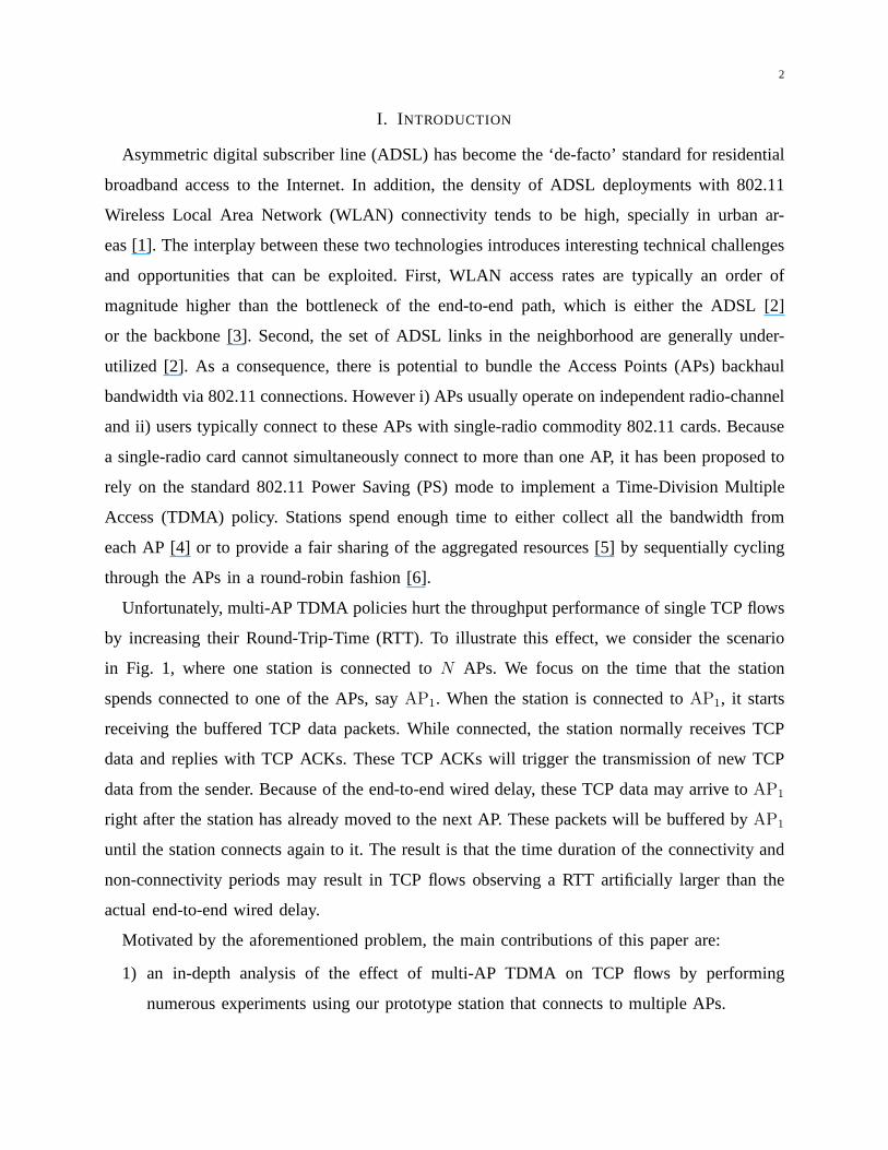
Unfortunately, multi-AP TDMA policies hurt the throughputperformance of single TCP flows

by increasing their Round-Trip-Time (RTT). To illustrate this effect, we consider the scenario

in Fig. 1, where one station is connected toN APs. We focus on the time that the station

spends connected to one of the APs, sayAP1. When the station is connected toAP1, it starts

receiving the buffered TCP data packets. While connected, the station normally receives TCP

data and replies with TCP ACKs. These TCP ACKs will trigger the transmission of new TCP

data from the sender. Because of the end-to-end wired delay,these TCP data may arrive toAP1

right after the station has already moved to the next AP. These packets will be buffered byAP1

until the station connects again to it. The result is that thetime duration of the connectivity and

non-connectivity periods may result in TCP flows observing aRTT artificially larger than the

actual end-to-end wired delay.

Motivated by the aforementioned problem, the main contributions of this paper are:

1) an in-depth analysis of the effect of multi-AP TDMA on TCP flows by performing

numerous experiments using our prototype station that connects to multiple APs.

3

����������������������������

����������������������������

End Connection Station

TCP Data N

Leave PS

TCP ACK N

TCP Data N+1

TCP Data N+1

TCP ACK N

Leave PS

Enter PS

Duty Cycle

Wireless Period

AP Queue Delay

End−to−End

Wired Delay

AP1

Fig. 1. Relation between TCP congestion control and time-division access to multiple APs.

2) an analytical model that correlates the TCP congestion control with the multi-AP TDMA

policy.

3) a cost-efficient resource allocation algorithm, namedmin-max disconnection time, that

distributes the time spent by the station to the APs in minislots (part of the TDMA slot)

to minimize the total disconnection time from the APs.

We evaluate our model and show that it accurately fits the experimental results. We further

study the algorithm via extensive simulations and we show that it performs very close to the

theoretical upper bound. The rest of the paper is organized as follows. Section II reviews related

work, and Section III presents our prototype implementation of multi-AP TDMA used in the

experimental tests. Then, Section IV investigates the performance degradation of TCP on the

multi-AP TDMA scenario, and it introduces an accurate analytical model. Section V validates

the analytical model via both experiments and simulations.The resource allocation algorithm is

introduced and validated in Section VI. Finally Section VIIconcludes the paper.

II. RELATED WORK

The need for 802.11 resource allocation schemes has been extensively studied in the litera-

ture [7]–[9]. Many of the proposed schemes rely on either non-standard compliant features [10],

or completely develop an entire new MAC protocol [11]. Both strategies may be undesirable, and

4

so we avoid them. Given that, the resource allocation schemethat more closely relates to ours

is [12], that studied the problem of absence of application-specific 802.11 resource allocation

schemes. As a solution, they designed and implemented an overlay MAC layer (OML) to divide

the time into slots of equal size. Then, they used a distributed algorithm to allocate the slots across

the competing nodes, where each competing node receives a number of slots proportional to its

weight function. However, the authors let as an open issue the understanding of the increased

delay for TCP flows in presence of the slotted mechanism [12].

Although overlay solutions are easy to be implemented, theyare often sub-optimal and difficult

to scale because of the overlapping and duplication of similar functionalities at different layers

(e.g. in the driver and in the card firmware). The VirtualWiFiproject [6] proposed an architecture

that abstracts a single 802.11 WLAN card to appear as multiple virtual clients to the user. Each

client instance adopts standard PHY/MAC protocols, but it can be separately configured at the

driver level. An interesting application was the idea of connecting to multiple APs through a

single radio interface. The authors rely on the 802.11 PowerSave (PS) mode feature to switch

among different 802.11 WLAN nodes in a time-division fashion. A station can inform the current

802.11 WLAN node that it is going into PS mode — so that it can buffer packets directed to

it — and switch the radio-frequency to other 802.11 WLAN nodes, only to come back to the

original node before the PS period expires.

Based on the above PS mechanism, FatVAP [4] studied the problem of ADSL bandwidth

aggregation via wireless connectivity. The authors introduced a local scheduler that computes

the percentage of time to dedicate to each AP in order to maximize the aggregate throughput

at each client station. The solution leverages on the fact that the high speed wireless card at

the station needs to be connected to each AP for a short periodof time in order to collect

all the pending data. THEMIS [5] reformulated the problem considering that gross unfairness

would be generated in the above setting. Their approach achieved weighted proportional fairness

and they experimentally validated it with a multistory building and real ADSLs, showing that

it outperformed previous solutions. However, both FatVAP and THEMIS do not explore TCP

latency-related problems for single TCP flows. They essentially limited the analysis to scenarios

with sufficient number of TCP flows, such that the ADSL bandwidth is saturated, or with short-

lived TCP flows, where the congestion control phase does not trigger. Finally, Juggler [13]

proposed an architecture similar to one in [4] and it focusedon the support of a seamless

5

Internet

ADSL/Cable

Line 1

ADSL/Cable ADSL/Cable

Line 2 Line 3

Wi−Switcher Station

AP2 AP3

V STA1 V STA2 V STA3

AP1

(a) Topology.

t

VSTA3 VSTA1 VSTA3VSTA1

Wireless Period

Duty Cy le 1 Duty Cy le 1Duty Cy le 3 Duty Cy le 3

VSTA2 VSTA2

Duty Cy le 2 Duty Cy le 2

(b) Relation between duty cycle and wireless period.

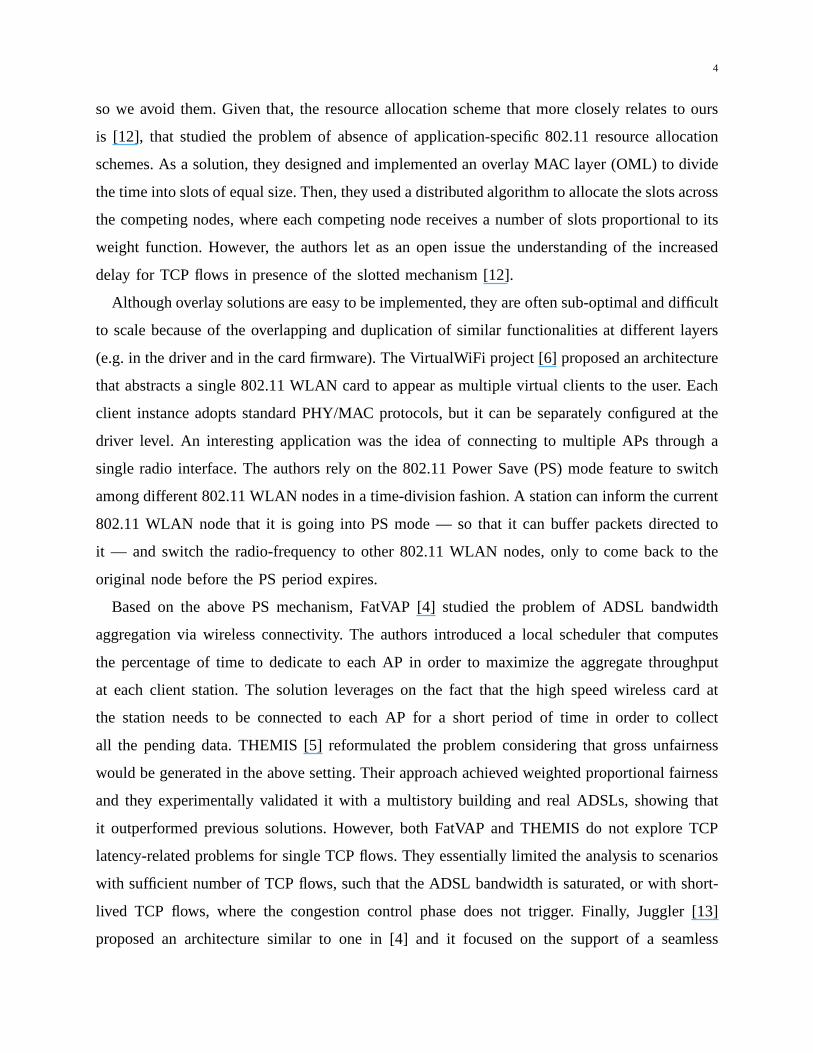
Fig. 2. Time Division Access to Multiple APs

hand-off between WLAN APs.

III. CONNECTING TO MULTIPLE APS WITH OFF-THE-SHELF HARDWARE

In this section, we briefly describe WiSwitcher [14], the experimental 802.11 station that we

have implemented and it will be used in the rest of this paper as the basis for the experimental

tests.

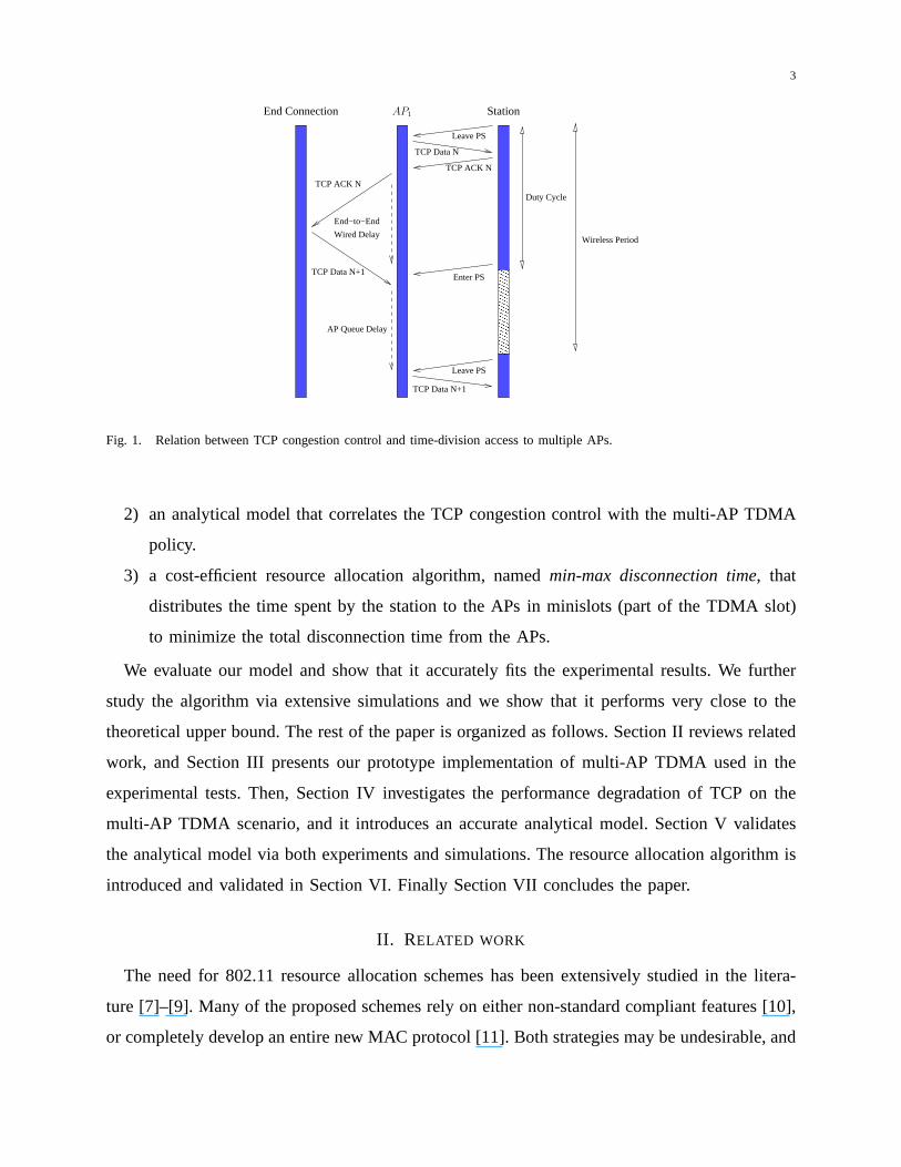
In WiSwitcher, the wireless driver of the single radio interface isvirtualized, i.e., it appears as

independent Virtual STAtions (VSTAi) associated to their respective Access PointsAPi. Each

VSTAi connects to Internet viaAPi, regardless of theAPi radio-frequency. Let us consider

the scenario with one station in Fig. 2(a), connected to three APs. In this example, WiSwitcher

configures3 virtual stationsVSTA1, VSTA2 andVSTA3. Each of these VSTAs connects to one

ADSL via its AP in range.

As we can see in Fig. 2(b), WiSwitcher assigns the control of the card to aVSTAi for a given

percentage of time, calledduty cyclefi (with∑

i fi = 1). During this time,VSTAi transmits and

receives frames using theAPi backhaul, while the other VSTAs (and the corresponding APs)

can only buffer packets. We denotewireless periodT as the amount of time to cycle through

all the VSTAs. A summary of the main variables used in this section and the rest of the paper

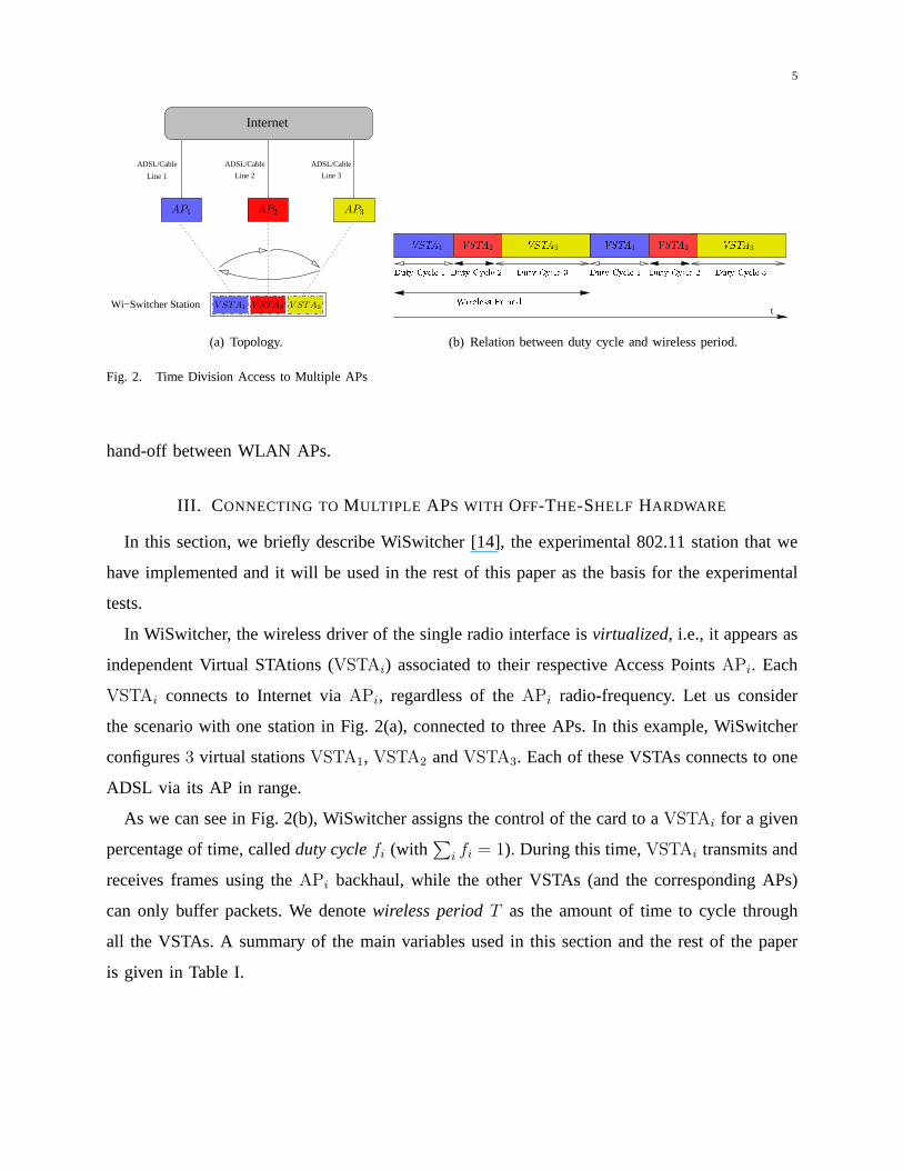
is given in Table I.

6

APi i-th AP

N Number of AP backhauls

T (ms) Wireless period

VSTAi i-th Virtual STAtion, associated toAPi

di End-to-end wired delay

fi (≤ 1) Duty cycle for thei-th virtual station

gi (≥ 1) Number of slots for thei-th virtual station

G Total number of slots

Cj Disconnection cost for thej-th slot

SlotTime Minimum slot size

TABLE I

MAIN VARIABLES USED.

A. MAC Protocol

WiSwitcher manages the multiple backhaul connections relying on the 802.11 PS mechanism.

Particularly, referring to the example in Fig 2(b):

1) During the reserved duty cycle,VSTA1 transmits and receives data according to the 802.11

Distributed Coordination Function (DCF) protocol. The other VSTAs are dormant in PS

mode, and hence they (and the corresponding APs) can only buffer packets.

2) When the duty cycle expires,VSTA1 sends a frame to informAP1 that is going to PS

mode and waits for its MAC ACK. According to the 802.11 protocol, AP1 starts to buffer

the packets directed to it.

3) WiSwitcher assigns the control of the card toVSTA2 and switches to theAP2 radio-

frequency.

4) VSTA2 sends a frame to announce that it can send and receive traffic and it waits for its

MAC ACK.

5) The process continues until the station has cycled through all theVSTAs (a wireless period

T ).

In the implementation, we incur in a channel-switching cost— i.e. the time where WiSwitcher

cannot send and receive any traffic — of1.2ms for uplink traffic and1.5ms for downlink traffic.

This cost is less than half of the one obtained in the time-division implementation given in [4],

7

[13]. This result has been achieved using 802.11 standard-compliant solutions, such as a MAC

virtual queue per AP, and an efficient management of a hardware buffer size of one (1) data

packet. The bulk of the cost of WiSwitcher is caused by the hardware operation delay, which

is in the order of800µsec in our Atheros chipset-based cards. This cost is hardware dependent

and in other chipset implementations is reduced to200− 500µsec [13].

Furthermore, the implementation achieves a fine-grained timing at MAC/PHY level, thus

avoiding any additional variance of the delay in the packet transmission, and it considers an

independent instance of the rate selection algorithm for each VSTA. This allows us to connect

to APs with different link qualities. The reader is referredto [14] for an in-depth description of

the MAC implementation.

B. Network Layer Functionalities

At the network layer, three functionalities are needed:

Scheduler: it calculates the percentage of time (duty cycle) to spend on each AP in order to

maximize some utility function. In this work, the duty cycles are fixed via user-space commands.

Load balancer: it assigns the new TCP flow from the upper layers to the different VSTAs so

that the total load received from each AP maintains the proportions indicated by the scheduler.

Since the load balancer is not the main objective of this work, we use the same per-flow basis

scheduler presented in [4].

Reverse-NAT: In order to guarantee transparency to higher layers, we implement a reverse-

network address translation (NAT) module with two functions: i) ensure that the packets leave

the host with the correct source IP address (i.e. the one corresponding to the outgoing VSTA, as

assigned by the AP) and ii) that the incoming packets are presented to the OS with the expected

IP address, a dummy IP address in our implementation. Reverse-NAT modules were also present

in [4] and [13].

IV. TCP OVER MULTI -APS TDMA

In this section, we first show an experimental test that enlightens the correlation between the

end-to-end throughput and the delay added by the TDMA policy, and then we introduce an

analytical model that characterizes the TCP RTT for a station connected to multiple APs. The

8

20 40 60 80 100 120 1400

1

2

3

4

5

6

7

8

9

10

End−to−end wired delay [ms]

Thr

ough

put [

Mbp

s]

Throughput variation with delay

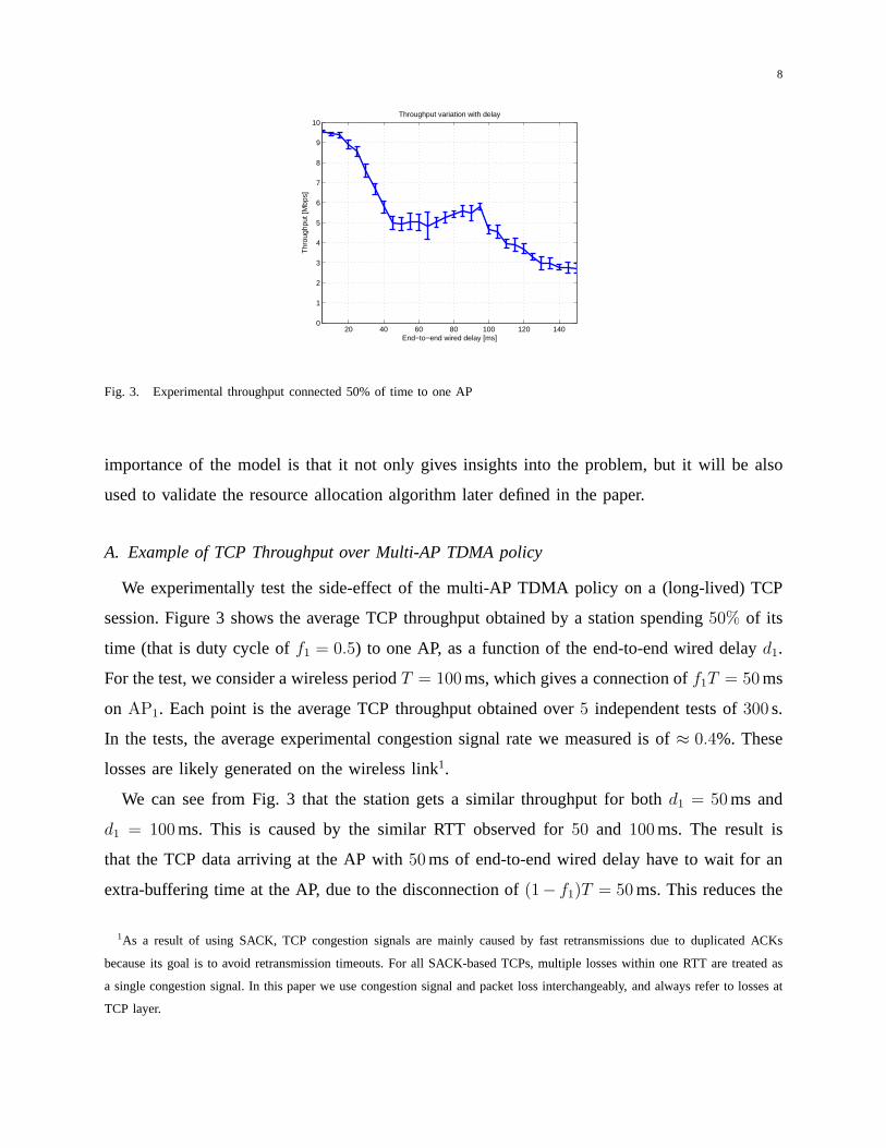
Fig. 3. Experimental throughput connected 50% of time to oneAP

importance of the model is that it not only gives insights into the problem, but it will be also

used to validate the resource allocation algorithm later defined in the paper.

A. Example of TCP Throughput over Multi-AP TDMA policy

We experimentally test the side-effect of the multi-AP TDMApolicy on a (long-lived) TCP

session. Figure 3 shows the average TCP throughput obtainedby a station spending50% of its

time (that is duty cycle off1 = 0.5) to one AP, as a function of the end-to-end wired delayd1.

For the test, we consider a wireless periodT = 100ms, which gives a connection off1T = 50ms

on AP1. Each point is the average TCP throughput obtained over5 independent tests of300 s.

In the tests, the average experimental congestion signal rate we measured is of≈ 0.4%. These

losses are likely generated on the wireless link1.

We can see from Fig. 3 that the station gets a similar throughput for both d1 = 50ms and

d1 = 100ms. This is caused by the similar RTT observed for50 and 100ms. The result is

that the TCP data arriving at the AP with50ms of end-to-end wired delay have to wait for an

extra-buffering time at the AP, due to the disconnection of(1− f1)T = 50ms. This reduces the

1As a result of using SACK, TCP congestion signals are mainly caused by fast retransmissions due to duplicated ACKs

because its goal is to avoid retransmission timeouts. For all SACK-based TCPs, multiple losses within one RTT are treated as

a single congestion signal. In this paper we use congestion signal and packet loss interchangeably, and always refer to losses at

TCP layer.

9

throughput observed by the TCP flow ford1 = 50ms. More exactly, there are small valleys in

the throughput: a disconnection of50ms increases the buffer size of the AP. Further increasing

the end-to-end wired delay from50 to 100ms, there is a higher and higher probability that

downlink packets will arrive at the AP when the station is connected to it. This will reduce the

buffering time at the AP (and thus the observed RTT), that will deliver the packets in a shorter

time, with a slight increase of the throughput2.

B. Modeling the TCP RTT over Multi-AP TDMA

We can model the dependency of the TCP RTT on the end-to-end delay and the duty cycle by

observing all the possible cases in which TDMA affects the observed RTT. In what follows,

we consider the uplink case (e.g. the VSTA is sending data to aremote server), but it is

straightforward to see that the RTT computations are symmetric for both the uplink and downlink

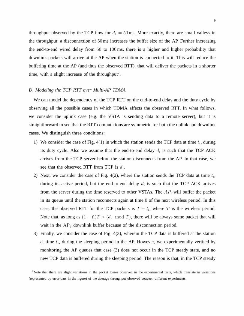
cases. We distinguish three conditions:

1) We consider the case of Fig. 4(1) in which the station sendsthe TCP data at timeti, during

its duty cycle. Also we assume that the end-to-end delaydi is such that the TCP ACK

arrives from the TCP server before the station disconnects from the AP. In that case, we

see that the observed RTT from TCP isdi.

2) Next, we consider the case of Fig. 4(2), where the station sends the TCP data at timeti,

during its active period, but the end-to-end delaydi is such that the TCP ACK arrives

from the server during the time reserved to other VSTAs. TheAPi will buffer the packet

in its queue until the station reconnects again at time0 of the next wireless period. In this

case, the observed RTT for the TCP packets isT − ti, whereT is the wireless period.

Note that, as long as(1− fi)T > (di mod T ), there will be always some packet that will

wait in theAP2 downlink buffer because of the disconnection period.

3) Finally, we consider the case of Fig. 4(3), wherein the TCPdata is buffered at the station

at time ti, during the sleeping period in the AP. However, we experimentally verified by

monitoring the AP queues that case (3) does not occur in the TCP steady state, and no

new TCP data is buffered during the sleeping period. The reason is that, in the TCP steady

2Note that there are slight variations in the packet losses observed in the experimental tests, which translate in variations

(represented by error-bars in the figure) of the average throughput observed between different experiments.

10

���������������������������������

���������������������������������

���������������������������������

���������������������������������

��������������������������������������������

TCP ACK

TCP Data

(2)

(3)

(1)TCP ACK

TCP Data

TCP Datadi

di

fi · T

T=wireless period

ti

ti

ti

Fig. 4. Model of the relation between TCP congestion controland duty cycle

state case, new TCP data can only be sent when a TCP ACK is received from the server.

But as we have seen, the TCP ACKs can only arrive to the stationwhen it is connected

to the AP.

Finally, in order to take into account that the station takessome time for processing and

transmitting the TCP ACKs, as verified experimentally, we consider that: i) the TCP ACKs

arrive exponentially distributed over the duty cycle, because there is a high probability that

some TCP ACK is waiting in theAPi downlink buffer when the station re-connects to it (in the

beginning of a duty cycle) ii) one TCP DATA is sent right afterthe reception of a TCP ACK.

This assumption considers the case when, in average and steady state, throughput does not either

increase or decrease iii) WhenfiT is very small, some of the TCP data scheduled during the

connection period will inevitably be sent at the next connectivity period, due to buffering delay.

Based on these assumptions, we statistically calculate theRTT distribution, considering as input

the wireless periodT , the duty cyclefi and the end-to-end delaydi. Despite the simplicity of

the model, Section V-A will show that the model matches the experimental results.

Mapping the modeled TCP RTT to Throughput:Although a wide variety of TCP algorithms

are used on the Internet, the current most popular implementation is TCP Reno [15]. Then, in

order to map the RTT given by the model to throughput, we use the Mathis TCP model [16],

which is intended to predict TCP end-to-end throughput as:BW ≤ MSSRTT

· 1√p, whereRTT is

the Round-Trip-Time observed by the station,MSS is the TCP Maximum Segment Size andp

11

is the packet loss rate3.

V. EVALUATION

In this section:

• we validate the accuracy of the TCP RTT model presented in theprevious section, comparing

it with experimental results.

• we show that long disconnection time severely affects the TCP throughput.

• we demonstrate that, for any duty cycle, the best strategy isto reduce the wireless period

T as much as possible.

• we show that the selection of the wireless periodT must be done based on the smallest

duty cyclemini fi of the station.

In what follows we discuss the details of the experimental and simulation setup.

Experimental setup In each controlled test, we use laptops with Atheros-based chipsets

running WiSwitcher as described in Section III and off-the-shelf APs (Linksys) with DD-

WRT v24sp1 firmware. On the wireless station, automatic rateselection, wireless multimedia

extensions, and the RTS/CTS mechanism are disabled. In the experimental tests of this paper,

the 802.11 PHY rate is fixed to54Mbps. Other tests were performed in other configurations

(e.g. with automatic rate selection enabled), and showed similar results to the ones presented

in this paper. Any no-802.11 standard compliant features atthe MAC level were also disabled.

Our station use an hardware queue with best effort parameters.

For the transport layer, we use a Linux standard TCP Reno withSACK and delayed ACK

options enabled. TCP parameters are monitored using a modified version of the TCP probe kernel

module and the kernel patch Web100. For each test, we establish one TCP connection over an

AP backhaul4 and we collect statistics using theiperf tool. Regarding the wired connections,

we emulate the AP backhaul links through thetc Linux traffic shaper, varying the delay using

the netemtool.

3This model applies to long lived connections over nearly allimplementations of TCP Reno with SACK TCP. Note that, in

order to use this model, the packet loss rate should be smaller than2%, condition verified in all the experimental tests in this

paper.

4Note that the link utilization can increase establishing more than one TCP connection over each AP [14], which is out-of-

the-scope of this paper.

12

20 40 60 80 100 120 14020

40

60

80

100

120

140

160

180

200

220

End−to−end wired delay [msecs]

RT

T [m

secs

]Experimental RTT variation with delay (f1=0.5)

15ms no TX25ms no TX50ms no TX75ms no TX100% connected

(a) Experimental RTT

20 40 60 80 100 120 140

40

60

80

100

120

140

160

180

200

220

End−to−end wired delay [msec]

RT

T [m

sec]

Model of RTT variation with delay (f1=0.5)

15ms no TX25ms no TX50ms no TX75ms no TX100% connected

(b) Analytical RTT.

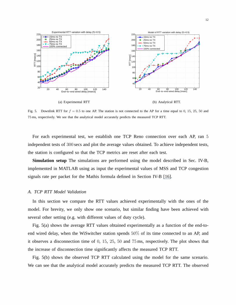
Fig. 5. Downlink RTT forf = 0.5 to one AP. The station is not connected to the AP for a time equal to 0, 15, 25, 50 and

75ms, respectively. We see that the analytical model accurately predicts the measured TCP RTT.

For each experimental test, we establish one TCP Reno connection over each AP, ran5

independent tests of300 secs and plot the average values obtained. To achieve independent tests,

the station is configured so that the TCP metrics are reset after each test.

Simulation setup The simulations are performed using the model described in Sec. IV-B,

implemented in MATLAB using as input the experimental values of MSS and TCP congestion

signals rate per packet for the Mathis formula defined in Section IV-B [16].

A. TCP RTT Model Validation

In this section we compare the RTT values achieved experimentally with the ones of the

model. For brevity, we only show one scenario, but similar finding have been achieved with

several other setting (e.g. with different values of duty cycle).

Fig. 5(a) shows the average RTT values obtained experimentally as a function of the end-to-

end wired delay, when the WiSwitcher station spends50% of its time connected to an AP, and

it observes a disconnection time of0, 15, 25, 50 and 75ms, respectively. The plot shows that

the increase of disconnection time significantly affects the measured TCP RTT.

Fig. 5(b) shows the observed TCP RTT calculated using the model for the same scenario.

We can see that the analytical model accurately predicts themeasured TCP RTT. The observed

13

20 40 60 80 100 120 1400

1

2

3

4

5

6

7

8

9

10

End−to−end wired delay [msecs]

Thr

ough

put [

Mbp

s]Experimental throughput variation with delay (f1=0.5)

15ms no TX25ms no TX50ms no TX75ms no TX

(a) Throughput with50% of connection (f1 = 0.5) to AP1.

20 40 60 80 100 120 1400

0.5

1

1.5

2

2.5

3

Thr

ough

put [

Mbp

s]

End−to−end wired delay [msecs]

Experimental throughput variation with delay (f1=0.1)

135ms no TX225ms no TX450ms no TX675ms no TX

(b) Throughput with10% of connection (f1 = 0.1) to AP1.

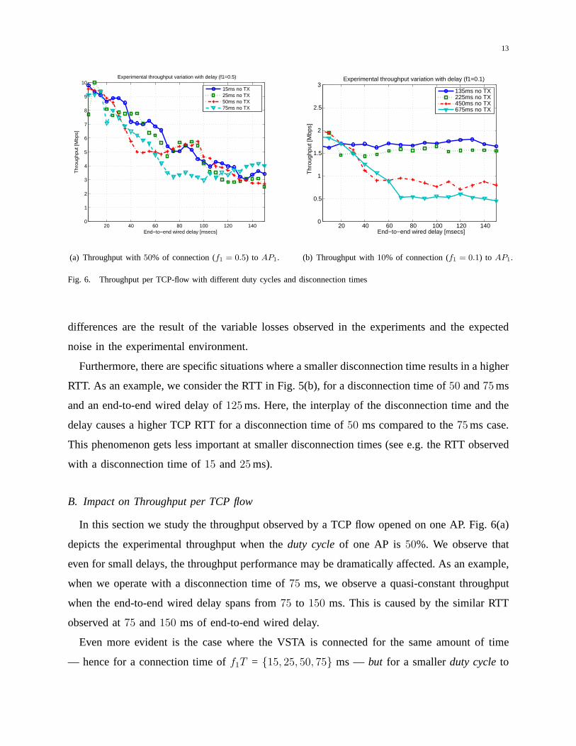
Fig. 6. Throughput per TCP-flow with different duty cycles and disconnection times

differences are the result of the variable losses observed in the experiments and the expected

noise in the experimental environment.

Furthermore, there are specific situations where a smaller disconnection time results in a higher

RTT. As an example, we consider the RTT in Fig. 5(b), for a disconnection time of50 and75ms

and an end-to-end wired delay of125ms. Here, the interplay of the disconnection time and the

delay causes a higher TCP RTT for a disconnection time of50 ms compared to the75ms case.

This phenomenon gets less important at smaller disconnection times (see e.g. the RTT observed

with a disconnection time of15 and25ms).

B. Impact on Throughput per TCP flow

In this section we study the throughput observed by a TCP flow opened on one AP. Fig. 6(a)

depicts the experimental throughput when theduty cycleof one AP is50%. We observe that

even for small delays, the throughput performance may be dramatically affected. As an example,

when we operate with a disconnection time of75 ms, we observe a quasi-constant throughput

when the end-to-end wired delay spans from75 to 150 ms. This is caused by the similar RTT

observed at75 and150 ms of end-to-end wired delay.

Even more evident is the case where the VSTA is connected for the same amount of time

— hence for a connection time off1T = {15, 25, 50, 75} ms — but for a smallerduty cycleto

14

AP1, e.g.10% of its time. We can also see from Fig. 6(b) that the penalty inthroughput is more

severe as the disconnection time grows. For example, when the disconnection time is 675 ms,

the average throughput is more than three times smaller thanthe throughput achieved when the

disconnection time is135 or 225ms.

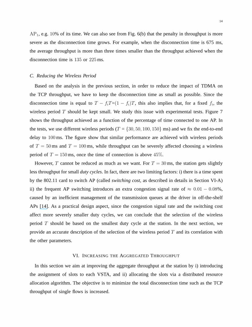
C. Reducing the Wireless Period

Based on the analysis in the previous section, in order to reduce the impact of TDMA on

the TCP throughput, we have to keep the disconnection time assmall as possible. Since the

disconnection time is equal toT − fiT=(1 − fi)T , this also implies that, for a fixedfi, the

wireless periodT should be kept small. We study this issue with experimental tests. Figure 7

shows the throughput achieved as a function of the percentage of time connected to one AP. In

the tests, we use different wireless periods (T = {30, 50, 100, 150} ms) and we fix the end-to-end

delay to100ms. The figure show that similar performance are achieved with wireless periods

of T = 50ms andT = 100ms, while throughput can be severely affected choosing a wireless

period ofT = 150ms, once the time of connection is above45%.

However,T cannot be reduced as much as we want. ForT = 30ms, the station gets slightly

less throughput for smallduty cycles. In fact, there are two limiting factors: i) there is a time spent

by the 802.11 card to switch AP (calledswitching cost, as described in details in Section VI-A)

ii) the frequent AP switching introduces an extra congestion signal rate of≈ 0.01 − 0.08%,

caused by an inefficient management of the transmission queues at the driver in off-the-shelf

APs [14]. As a practical design aspect, since the congestionsignal rate and the switching cost

affect more severely smaller duty cycles, we can conclude that the selection of the wireless

period T should be based on the smallest duty cycle at the station. In the next section, we

provide an accurate description of the selection of the wireless periodT and its correlation with

the other parameters.

VI. I NCREASING THEAGGREGATEDTHROUGHPUT

In this section we aim at improving the aggregate throughputat the station by i) introducing

the assignment of slots to each VSTA, and ii) allocating the slots via a distributed resource

allocation algorithm. The objective is to minimize the total disconnection time such as the TCP

throughput of single flows is increased.

15

20 25 30 35 40 45 50 55 600

1

2

3

4

5

6

7

% of time connected to AP1

Thr

ough

put [

Mbp

s]

Throughput vs % of time connected to AP1

Wireless period = 30msWireless period = 50msWireless period = 100msWireless period = 150ms

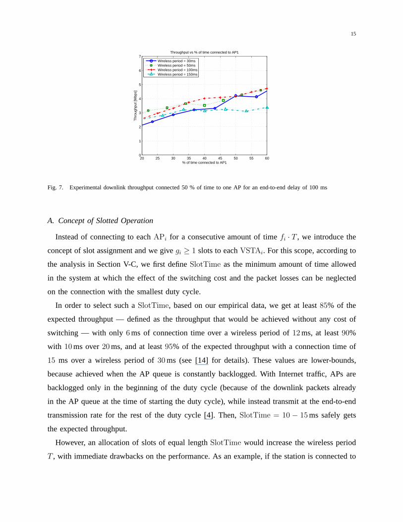
Fig. 7. Experimental downlink throughput connected 50 % of time to one AP for an end-to-end delay of 100 ms

A. Concept of Slotted Operation

Instead of connecting to eachAPi for a consecutive amount of timefi · T , we introduce the

concept of slot assignment and we givegi ≥ 1 slots to eachVSTAi. For this scope, according to

the analysis in Section V-C, we first defineSlotTime as the minimum amount of time allowed

in the system at which the effect of the switching cost and thepacket losses can be neglected

on the connection with the smallest duty cycle.

In order to select such aSlotTime, based on our empirical data, we get at least85% of the

expected throughput — defined as the throughput that would beachieved without any cost of

switching — with only6ms of connection time over a wireless period of12ms, at least90%

with 10ms over20ms, and at least95% of the expected throughput with a connection time of

15 ms over a wireless period of30ms (see [14] for details). These values are lower-bounds,

because achieved when the AP queue is constantly backlogged. With Internet traffic, APs are

backlogged only in the beginning of the duty cycle (because of the downlink packets already

in the AP queue at the time of starting the duty cycle), while instead transmit at the end-to-end

transmission rate for the rest of the duty cycle [4]. Then,SlotTime = 10 − 15ms safely gets

the expected throughput.

However, an allocation of slots of equal lengthSlotTime would increase the wireless period

T , with immediate drawbacks on the performance. As an example, if the station is connected to

16

two APs with scheduler outputf1 = 0.27 andf2 = 0.73, we would need27 slots forAP1 and73

slots onAP2. A SlotTime set to15 ms would result in a wireless period of15 · 100 = 1500ms,

which is computational inefficient.

Driven by the experiments and simulations of the previous section, we resolve this problem

with the following principles:

• we calculate the wireless period as:T = SlotTimemini fi

, that is, the procedure reduces the wireless

periodT , based on the smallest duty cycle of the station (as demonstrated in Section V-C).

• we derive the number of slots locally assigned to eachVSTAi as:gi = ⌊(fiT )/SlotTime⌋,for a total number of slots ofG =

∑

gi.

• we determine the slot size perVSTAi as:SlotTimei =fiT

gi. This may give slots of different

sizes among differentVSTAs.

Note that the solution can be transparently applied to the systems proposed in [4], [5], [13],

considering the different switching costs of these systemsto computeSlotTime.

Once selectedT , {gi} and {SlotTimei}, our objective is to construct a resource allocation

algorithm that, given the set of duty cyclesfi provided by the upper-layer scheduler, it assigns the

set of slots to theAPs in order to minimize the overall disconnection time for all the APs. For a

rigorous analysis of the resource allocation algorithms, some definition is needed, as introduced

in the next paragraph.

Disconnection Cost Let us defineSi = [Si(1), Si(2), . . . Si(gi)] the vector that indicates the

slot positions in the range[1, G] for VSTAi, with Si(gi+1) = Si(1) andSi(l) 6= Sj(m) for any

i, j = 1, . . . N , with i 6= j, l = 1, 2, . . . gi andm = 1, 2, . . . gj. Besides, we define the cost (slot

duration) of each slot as the slot size of theVSTAi that uses the slot:

CSi(l) = SlotTimei ∀i.

In order to measure the disconnection cost of theVSTAi during two transmissions in the slots

Si(l) andSi(l+1) we take into account the costs of the intermediate slotsCSi(l)+1, . . . CSi(l+1)−1.

Therefore, we introduce the following cost function:

ci,l =

Si(l+1)−1∑

j=Si(l)+1

Cj l = 1, 2, . . . gi

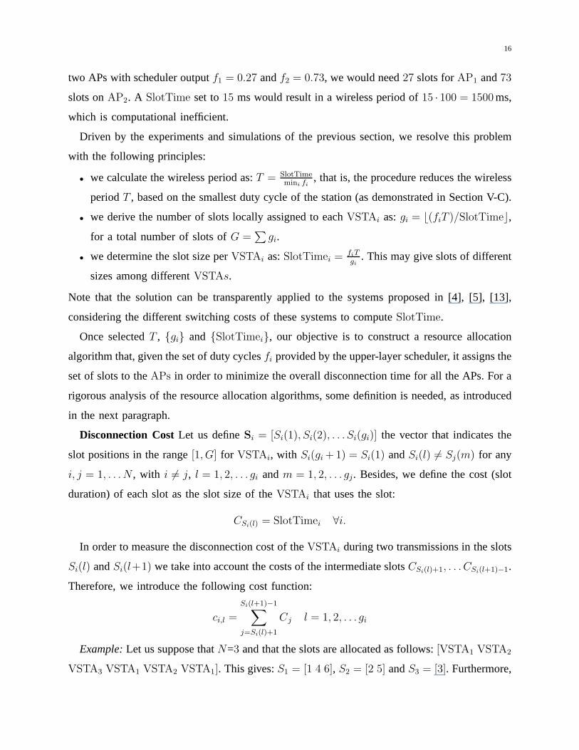
Example:Let us suppose thatN=3 and that the slots are allocated as follows:[VSTA1 VSTA2

VSTA3 VSTA1 VSTA2 VSTA1]. This gives:S1 = [1 4 6], S2 = [2 5] andS3 = [3]. Furthermore,

17

we suppose thatSlotTime3 = 10 ms, SlotTime1 = 12 ms andSlotTime2 = 15 ms. Then, we

calculate the disconnection cost betweenS1(1)=1 andS1(2)=4 asc1,1 = C2+C3 = 15+10 = 25

ms.

B. Resource allocation algorithm

We now present three different, fully decentralized, slot allocation mechanisms with different

performance and computational costs that aim to reduce the impact that the multi-AP TDMA

has on single TCP flows5.

Blind Resource Allocation. We have seen in Section V-A that a multi-AP TDMA policy

increases the observed RTT of the TCP packets. We have also seen that this increase is exactly

the disconnection time in the worst case. In other terms, forVSTAi, and given an allocation

that produces a disconnection time ofmaxl=1,2,...gi

ci,l, we would have

RTTi = di + maxl=1,2,...gi

ci,l.

The TCP throughput achieved by the above allocation can be approximated as

MSS

[di +maxl

ci,l] ·√pi,

whereMSS and pi are the parameters of the Mathis model defined in Section IV-B[16]. It

follows that, in order to minimize the throughput penalty caused by disconnection, we need to

solve the following problem:

minN∑

i

MSS

di ·√pi

− MSS

[di +maxl

ci,l] ·√pi

. (1)

The slot assignment obtained from solving (1) depends on thecorrect estimation of the

loss rates{pi} and end-to-end delays{di}. In a realistic deployment, an accurate prediction

of these values may be not available. In the absence of any end-to-end delay information we can

5We also tested an allocation mechanism with random assignment of the slots, using as a constraint that each slot is assigned

to a givenVSTAi with a probability equal tofi. Although this random assignment may decrease the buffering time at the AP in

certain configurations, we found that it generally increases the jitter observed by TCP, and then reduces the observed downlink

throughput.

18

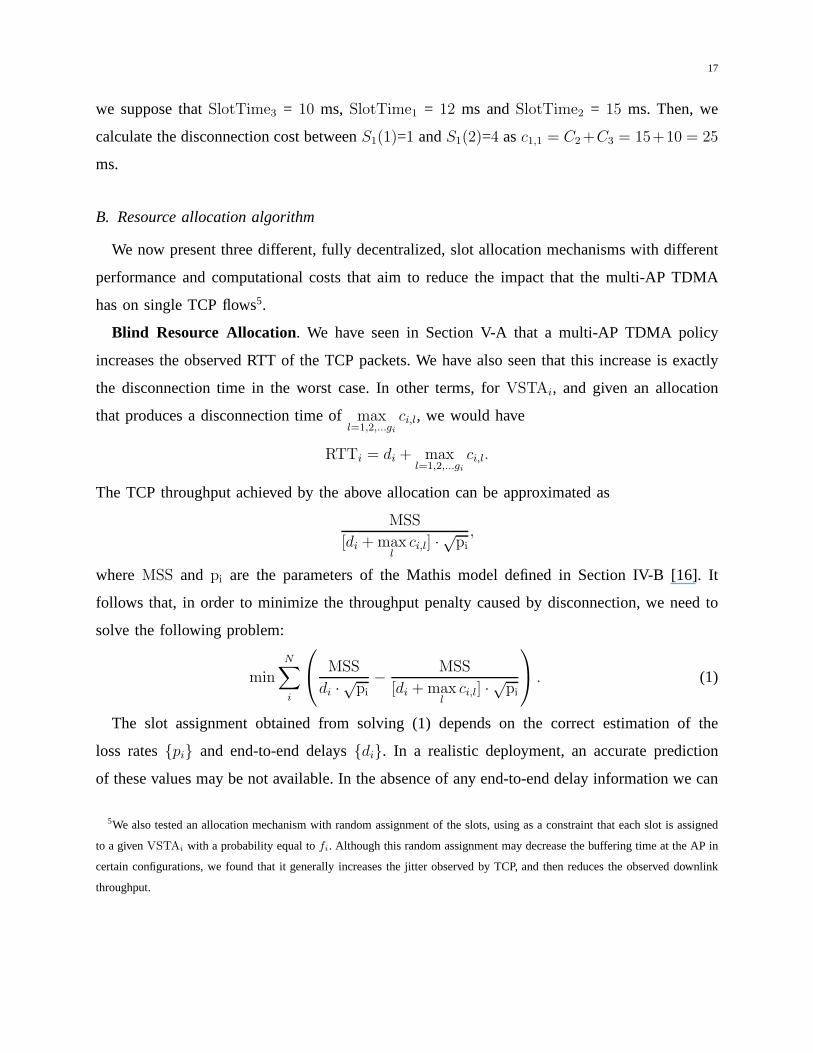
reformulate the problem simply as the minimization of the inverse of the maximum disconnection

times as follows:

maxSi(l)

N∑

i

1/(maxl

ci,l)

s.t.G∑

i=1

Ci = T

fiT = gi · SlotTimei ∀iSi(l) ∈ {1, G} ∀i, l,

(2)

where the variablesCi, SlotTime, fi andgi are defined in Table I.

Min-Max Disconnection Time Allocation Algorithm. The blind resource allocation algo-

rithm defined above can be prohibitively expensive. In orderto reduce its complexity, we define

a min-max disconnection timeheuristic approach. This algorithm considers that, in average,

the TCP throughput is more severely affected by the amount oftime that eachVSTAi is not

connectedto the correspondingAPi. Therefore, the algorithm tries to minimize the disconnection

time, starting with the connection with the largest duty cycle (i.e., the AP backhaul with the

highest utilization). The algorithm operates as follows:

1) First, it allocates the slots to theVSTA with max(gi).

2) Next, theVSTAs with lower number of slots will be served one by one. At each step, the

selectedi-th VSTAi analyzesonly the slots not previously assigned and it calculates the

vectorSi to satisfy the condition:min maxl=1,2,...gi

(Si(l + 1)− Si(l)), that is, it selects thegi

slots to minimize the maximum distance between each pair of consecutive slots assigned

to theVSTAi.

3) Finally, at the last step, the remaining set of slots are assigned to theVSTA with min(gi).

The lastVSTAi to allocate is the one with the smallest duty cycle. For that one,SlotTime

is already chosen such as its performance is not affected

Upper-bound We also calculate the upper-bound for the TCP aggregate throughput: for each

delay, we compute the TCP aggregate throughput for all the feasible solutions and select the

one that achieves the maximum throughput. Note that this upper bound can not be calculated in

practice and we include it for comparison purposes.

19

C. Simulation results

We now evaluate the above algorithms — and particularly the aggregate throughput achieved

by the min-max disconnection timeallocation — via simulations in different scenarios: i) high

number of APs ii) VSTAs with different duty cycle and delay and iii) different slot size per

VSTA. In the tests, we consider one long-lived TCP flow for each VSTA and we suppose that

the end-to-end communication is limited by the RTT delay, sothat we do not reach the maximum

capacity of the end-to-end path. For each test, we generate10000 samples of RTT6 and we use

a congestion signal rate of0.32%, as the one measured experimentally by connecting to one AP

in range with high signal-to-noise ratio, and measuring theaverage number of congestion signals

per acknowledged packet7. Note that each TCP flow experiences a different RTT, according to

the specific duty cycle and slots’ assignment. Note also thatmore TCP flows may be sent per

AP and other congestion signal rates may be used (even higher, according to the link quality

and the 802.11 PHY rate), but do not add a new contribution to this section.

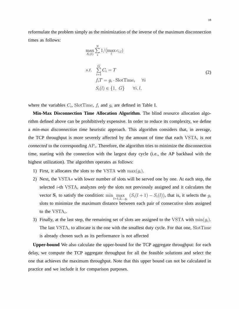
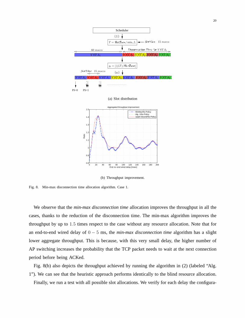
Case 1: High number of APs. Fig. 8(a) shows a station is connected to5 APs, with the

scheduler selecting the following duty cycles:f1 = 0.5, f2 = 0.125, f3 = 0.125, f4 = 0.125,

f5 = 0.125. The corresponding number of slots, based on the slot calculation presented in Section

VI.A, are g1 = 4, g2 = 1, g3 = 1, g4 = 1, g5 = 1, and the total number of slots isG = 8. In

the model, we useSlotTime = 15ms, which gives a wireless period of15ms ·8 slots= 120ms.

The algorithm minimizes the time without transmission allocating first the slot toVSTA1, then

to VSTA2, VSTA3, VSTA4, andVSTA5.

Fig. 8(b) depicts the throughput improvement versus the end-to-end delay, obtained comparing

the proposed allocation algorithm (labeled “MinMax”) withno resource allocation (labeled “No

Policy”), that is, spending consecutive 60 ms onVSTA1, and then15ms onVSTA2, VSTA3,

VSTA4, andVSTA5, sequentially.

6Similar results were achieved with1000 samples. More samples then10000 can be used, but it would adversely affect the

simulation time, without impact on the results.

7We use the congestion signal rate connecting to one AP, because, as discussed in Section V-C, current off-the-shelf APs

implementations add at each AP a certain packet loss rate, that may limit the performance in experimental implementations.

The reader is referred to [14] for more details. In this work,we do not consider these implementation issues, (that, however, do

not currently allow a validation of the resource allocationalgorithm with real experiments), and assume that the limiting factor

is the time spent by the 802.11 card to switch AP.

20

PS=1PS=0

Scheduler

SlotTime=15 msecs

V STA1

gi = ⌊(fiT )/SlotTime⌋

V STA2

V STA2

V STA4 V STA5V STA1

V STA3 V STA4 V STA5

V STA3V STA1 V STA1V STA1

60 msecs

T = SlotTime/ mini fi

Dis onne tion Time for V STA1

SlotTime=15 msecs

{fi}

{gi}

(a) Slot distribution

0 20 40 60 80 100 120 140 160 180 2000.8

0.9

1

1.1

1.2

1.3

1.4

1.5

End−to−end wired delay [msec]

Rat

io

Aggregated throughput improvement

MinMax/No PolicyAlg. 1/No PolicyUpper Bound/No Policy

(b) Throughput improvement.

Fig. 8. Min-max disconnection time allocation algorithm. Case 1.

We observe that themin-max disconnection timeallocation improves the throughput in all the

cases, thanks to the reduction of the disconnection time. The min-max algorithm improves the

throughput by up to1.5 times respect to the case without any resource allocation. Note that for

an end-to-end wired delay of0− 5 ms, themin-max disconnection timealgorithm has a slight

lower aggregate throughput. This is because, with this verysmall delay, the higher number of

AP switching increases the probability that the TCP packet needs to wait at the next connection

period before being ACKed.

Fig. 8(b) also depicts the throughput achieved by running the algorithm in (2) (labeled “Alg.

1”). We can see that the heuristic approach performs identically to the blind resource allocation.

Finally, we run a test with all possible slot allocations. Weverify for each delay the configura-

21

tion that achieves the upper bound, according to the methodology given in Section VI-B (labeled

“Upper Bound”). We observe that, despite the high cost and the need for an optimal calculation

of the end-to-end delay per connection and the packet loss rate, the upper bound algorithm

only slightly increases the aggregate throughput observedby the station respect to themin-max

disconnection timeapproach. The main reason behind this result is that the key parameter that

affects the end-to-end TCP throughput is the disconnectiontime from the AP, which is taken

into account in themin-max disconnection timeapproach, rather than the extra-buffering time

at the AP.

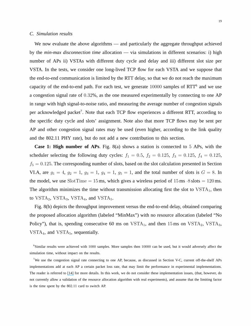
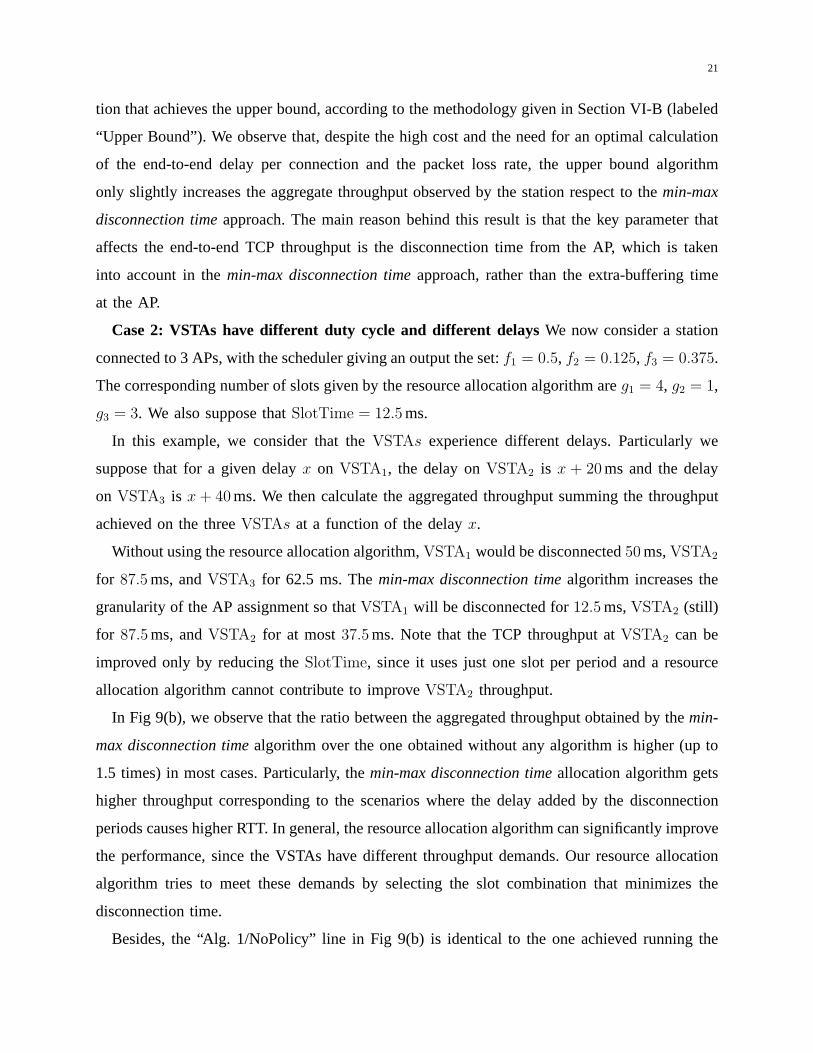
Case 2: VSTAs have different duty cycle and different delays We now consider a station

connected to 3 APs, with the scheduler giving an output the set: f1 = 0.5, f2 = 0.125, f3 = 0.375.

The corresponding number of slots given by the resource allocation algorithm areg1 = 4, g2 = 1,

g3 = 3. We also suppose thatSlotTime = 12.5ms.

In this example, we consider that theVSTAs experience different delays. Particularly we

suppose that for a given delayx on VSTA1, the delay onVSTA2 is x + 20ms and the delay

on VSTA3 is x+ 40ms. We then calculate the aggregated throughput summing thethroughput

achieved on the threeVSTAs at a function of the delayx.

Without using the resource allocation algorithm,VSTA1 would be disconnected50ms,VSTA2

for 87.5ms, andVSTA3 for 62.5 ms. Themin-max disconnection timealgorithm increases the

granularity of the AP assignment so thatVSTA1 will be disconnected for12.5ms,VSTA2 (still)

for 87.5ms, andVSTA2 for at most37.5ms. Note that the TCP throughput atVSTA2 can be

improved only by reducing theSlotTime, since it uses just one slot per period and a resource

allocation algorithm cannot contribute to improveVSTA2 throughput.

In Fig 9(b), we observe that the ratio between the aggregatedthroughput obtained by themin-

max disconnection timealgorithm over the one obtained without any algorithm is higher (up to

1.5 times) in most cases. Particularly, themin-max disconnection timeallocation algorithm gets

higher throughput corresponding to the scenarios where thedelay added by the disconnection

periods causes higher RTT. In general, the resource allocation algorithm can significantly improve

the performance, since the VSTAs have different throughputdemands. Our resource allocation

algorithm tries to meet these demands by selecting the slot combination that minimizes the

disconnection time.

Besides, the “Alg. 1/NoPolicy” line in Fig 9(b) is identicalto the one achieved running the

22

PS=1PS=0

SlotTime=12.5 msecs

V STA1

V STA1 V STA3

gi = ⌊(fi)T/SlotTime⌋

V STA2

V STA1V STA1 V STA3V STA1 V STA2V STA3V STA3

{gi}

Dis onne tion Time for V STA1

(a) Slot distribution.

0 20 40 60 80 100 120 140 160 180 2000.9

1

1.1

1.2

1.3

1.4

1.5

End−to−end wired delay [msec]

Rat

io

Aggregated throughput improvement

MinMax/No PolicyAlg. 1/No PolicyUpper Bound/No Policy

(b) Throughput improvement.

Fig. 9. Min-max disconnection time allocation algorithm. Case 2.

algorithm in (2), that needs280 runs to analyze all the feasible solutions, respect to the6

runs needed by themin-max disconnection timealgorithm. Finally, “Upper Bound/NoPolicy”

line shows that the throughput improvements achieved with the optimum solution (upper bound

algorithm) is negligible.

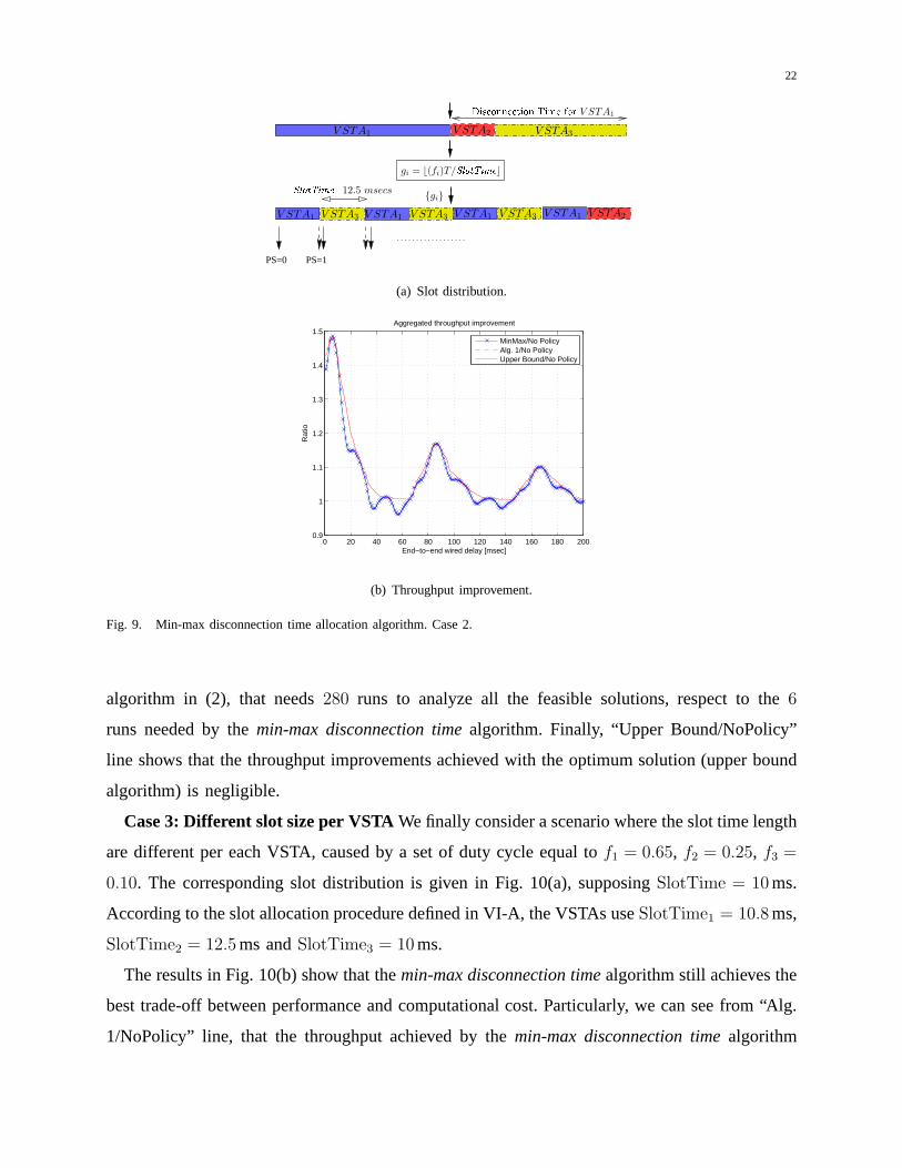
Case 3: Different slot size per VSTA We finally consider a scenario where the slot time length

are different per each VSTA, caused by a set of duty cycle equal to f1 = 0.65, f2 = 0.25, f3 =

0.10. The corresponding slot distribution is given in Fig. 10(a), supposingSlotTime = 10ms.

According to the slot allocation procedure defined in VI-A, the VSTAs useSlotTime1 = 10.8ms,

SlotTime2 = 12.5ms andSlotTime3 = 10ms.

The results in Fig. 10(b) show that themin-max disconnection timealgorithm still achieves the

best trade-off between performance and computational cost. Particularly, we can see from “Alg.

1/NoPolicy” line, that the throughput achieved by themin-max disconnection timealgorithm

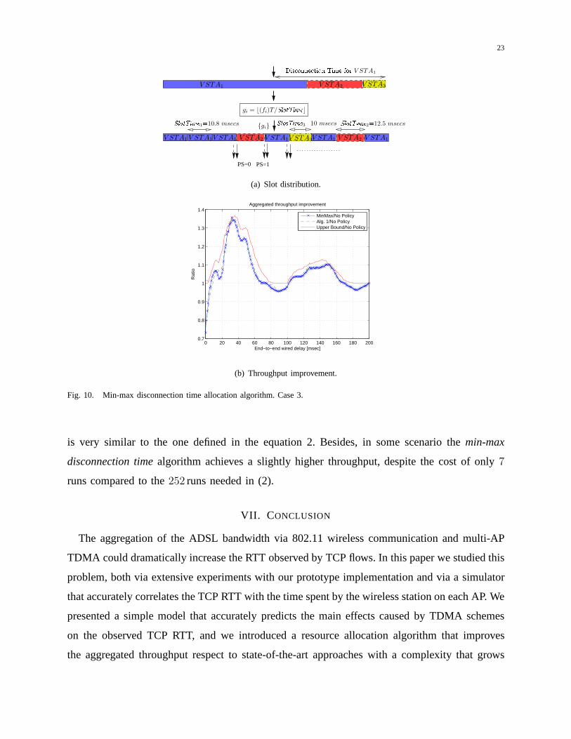
23

PS=0 PS=1

V STA1

gi = ⌊(fi)T/SlotTime⌋

{gi}

V STA2 V STA3

V STA2V STA1 V STA1V STA3V STA1 V STA1 V STA2 V STA1

SlotTime2=12.5 msecsSlotTime3=10 msecsSlotTime1=10.8 msecs

V STA1

Dis onne tion Time for V STA1

(a) Slot distribution.

0 20 40 60 80 100 120 140 160 180 2000.7

0.8

0.9

1

1.1

1.2

1.3

1.4

End−to−end wired delay [msec]

Rat

io

Aggregated throughput improvement

MinMax/No PolicyAlg. 1/No PolicyUpper Bound/No Policy

(b) Throughput improvement.

Fig. 10. Min-max disconnection time allocation algorithm.Case 3.

is very similar to the one defined in the equation 2. Besides, in some scenario themin-max

disconnection timealgorithm achieves a slightly higher throughput, despite the cost of only7

runs compared to the252 runs needed in (2).

VII. CONCLUSION

The aggregation of the ADSL bandwidth via 802.11 wireless communication and multi-AP

TDMA could dramatically increase the RTT observed by TCP flows. In this paper we studied this

problem, both via extensive experiments with our prototypeimplementation and via a simulator

that accurately correlates the TCP RTT with the time spent bythe wireless station on each AP. We

presented a simple model that accurately predicts the main effects caused by TDMA schemes

on the observed TCP RTT, and we introduced a resource allocation algorithm that improves

the aggregated throughput respect to state-of-the-art approaches with a complexity that grows

24

linearly with the number of APs. Our solution does not require modifications to the rest of the

network, and it can be applied to existing solutions that aggregate the AP backhaul bandwidth.

Furthermore, we showed that its throughput performance is very close to the theoretical upper

bound for a number of key scenarios. We believe that our approach will help to provide an

efficient solution to aggregate multiple AP backhauls independently of the type of TCP traffic.

REFERENCES

[1] D. Han, A. Agarwala, D. G. Andersen, M. Kaminsky, K. Papagiannaki, and S. Seshan, “Mark-and-sweep:

getting the ”inside” scoop on neighborhood networks,” inProceedings of the 8th ACM SIGCOMM conference

on Internet measurement, ser. IMC ’08. New York, NY, USA: ACM, 2008, pp. 99–104. [Online]. Available:

http://doi.acm.org/10.1145/1452520.1452532

[2] M. Siekkinen, D. Collange, G. Urvoy-keller, and E. W. Biersack, “Performance limitations of adsl users: A case study,”

in In Proceedings of the 8th Passive and Active Measurement Conference (PAM), 2007.

[3] G. Maier, A. Feldmann, V. Paxson, and M. Allman, “On dominant characteristics of residential broadband internet

traffic,” in Proceedings of the 9th ACM SIGCOMM conference on Internet measurement conference, ser. IMC ’09. New

York, NY, USA: ACM, 2009, pp. 90–102. [Online]. Available: http://doi.acm.org/10.1145/1644893.1644904

[4] S. Kandula, K. C.-J. Lin, T. Badirkhanli, and D. Katabi, “Fatvap: aggregating ap backhaul capacity to

maximize throughput,” in Proceedings of the 5th USENIX Symposium on Networked Systems Design and

Implementation, ser. NSDI’08. Berkeley, CA, USA: USENIX Association, 2008, pp. 89–104. [Online]. Available:

http://dl.acm.org/citation.cfm?id=1387589.1387596

[5] D. Giustiniano, E. Goma, A. Lopez Toledo, I. Dangerfield,J. Morillo, and P. Rodriguez, “Fair wlan backhaul aggregation,”

in Proceedings of the sixteenth annual international conference on Mobile computing and networking, ser. MobiCom ’10.

New York, NY, USA: ACM, 2010, pp. 269–280. [Online]. Available: http://doi.acm.org/10.1145/1859995.1860026

[6] R. Chandra and P. Bahl, “Multinet: Connecting to multiple ieee 802.11 networks using a single wireless card,” inINFOCOM

2004. Twenty-third AnnualJoint Conference of the IEEE Computer and Communications Societies, vol. 2. IEEE, 2004,

pp. 882–893.

[7] G. Athanasiou, T. Korakis, O. Ercetin, and L. Tassiulas,“Dynamic cross-layer association in 802.11-based mesh networks,”

in IEEE INFOCOM, Anhcorage, Alaska, USA, May 2007, pp. 2090–2098.

[8] L. Georgiadis, M. Neely, M. J. Neely, and L. Tassiulas,Resource allocation and cross-layer control in wireless networks.

Now Pub, 2006.

[9] G. Athanasiou, T. Korakis, O. Ercetin, and L. Tassiulas,“A cross-layer framework for association control in wireless mesh

networks,” IEEE Transactions on Mobile Computing, vol. 8, no. 1, pp. 65–80, Jan. 2009.

[10] C. Doerr, M. Neufeld, J. Fifield, T. Weingart, D. Sicker,and D. Grunwald, “Multimac - an adaptive mac framework for

dynamic radio networking,” inNew Frontiers in Dynamic Spectrum Access Networks, 2005. DySPAN 2005. 2005 First

IEEE International Symposium on, Nov., pp. 548–555.

[11] A. Sharma and E. M. Belding, “Freemac: framework for multi-channel mac development on 802.11 hardware,” in

Proceedings of the ACM workshop on Programmable routers forextensible services of tomorrow. ACM, 2008, pp.

69–74.

25

[12] A. Rao and I. Stoica, “An overlay mac layer for 802.11 networks,” in Proceedings of the 3rd international conference on

Mobile systems, applications, and services. ACM, 2005, pp. 135–148.

[13] A. J. Nicholson, S. Wolchok, and B. D. Noble, “Juggler: Virtual networks for fun and profit,”Mobile Computing, IEEE

Transactions on, vol. 9, no. 1, pp. 31–43, 2010.

[14] D. Giustiniano, E. Goma, A. Lopez, and P. Rodriguez, “Wiswitcher: an efficient client for managing

multiple aps,” in Proceedings of the 2nd ACM SIGCOMM workshop on Programmablerouters for extensible

services of tomorrow, ser. PRESTO ’09. New York, NY, USA: ACM, 2009, pp. 43–48. [Online]. Available:

http://doi.acm.org/10.1145/1592631.1592642

[15] W. R. Stevens, “Tcp slow start, congestion avoidance, fast retransmit, and fast recovery algorithms,” 1997.

[16] M. Mathis, J. Semke, J. Mahdavi, and T. Ott, “The macroscopic behavior of the tcp congestion avoidance algorithm,”

ACM SIGCOMM Computer Communication Review, vol. 27, no. 3, pp. 67–82, 1997.