Optimizing Edge Computing in 5G Networks Optimizing Edge Computing in 5G Networks Jinghui Jiang (4821998) MSc graduation committee Dr. ir. Eric Smeitink, Dr. ing. Edgar van Boven, Ir. Rogier Noldus, Dr. Qing Wang.

Welcome message from author
This document is posted to help you gain knowledge. Please leave a comment to let me know what you think about it! Share it to your friends and learn new things together.
Transcript

Optimizing Edge Computing in 5G Networks
Optimizing Edge Computing
in 5G Networks
Jinghui Jiang (4821998)
MSc graduation committee
Dr. ir. Eric Smeitink,
Dr. ing. Edgar van Boven,
Ir. Rogier Noldus,
Dr. Qing Wang.


Optimizing Edge Computing
in 5G Networks
Jinghui Jiang (4821998)
MSc graduation committee
Dr. ir. Eric Smeitink1,2,
Dr. ing. Edgar van Boven1,2,
Ir. Rogier Noldus1,3,
Dr. Qing Wang4.
1 Delft University of Technology
Faculty of Electrical Engineering, Mathematics, and Computer Science
Department of Network Architecture & Services
Mekelweg 4, 2628 CD Delft, The Netherlands
2 Koninklijke KPN N.V.
Maanplein 55, 2516 CK Den Haag, The Netherlands
3 Ericsson Telecommunicatie B.V.
Ericssonstraat 2, 5121 ML Rijen, The Netherlands
4 Delft University of Technology
Faculty of Electrical Engineering, Mathematics, and Computer Science
Embedded and Networked Systems (ENS) Group
Mekelweg 4, 2628 CD Delft, The Netherlands


Optimizing Edge Computing in 5G Networks
Preface
Preface
As 5G technology is developing at a high speed nowadays, edge computing starts to get
noticed again. Even though the origin of edge computing can be traced back to late 1990s,
there are some barriers which make the implementation of edge computing difficult and
costly in practice. With network function virtualization in 5G, the deployment of edge
computing needs to get close enough to the network edge to reduce latency and bandwidth
usage in order to meet the requirements derived from future use cases. Network function
virtualization brings flexibilities to edge computing as well as more optimization possibilities,
including reducing costs and investments of companies that provide edge computing
services and enhancing user experience and service qualities of edge computing. With
optimizations, edge computing can provide enhanced service quality (e.g. shorter service
latency, higher reliability, higher robustness, etc.) to users with a reasonably small amount
of investments. These improvements provided by optimizations are desired for both
customers and operators, and edge computing will get more attention, will develop faster
and will be more widely used.


Optimizing Edge Computing in 5G Networks
Acknowledgement
Acknowledgement
During the 11 months doing my master thesis, I received a lot of help in all aspects from my
supervisors, my colleagues and my family and friends.
First of all, I want to give thanks to my supervisors, Ir. Rogier Noldus, Dr. ing. Edgar van
Boven and Dr. ir. Eric Smeitink. Rogier is a principal architect at Ericsson Value-added Service
group. He is the one who offered me this opportunity to work with him at Ericsson on my
master thesis. He not only gave me this interesting topic about edge computing, but also
inspired me a lot during my thesis. Whenever I ran into problems, he always offered me help
and shared his brilliant ideas with me. Besides, he helped me with my thesis-related writing
and presentation, gave me suggestions on the structure as well as more detailed writing and
presenting skills. Edgar is an architect at KPN. He gave me a lot of instructions on writing and
structuring not only my thesis, but also my research proposal, my mid-term presentation, my
interview questions and my final presentation. Also, Edgar gave me nice suggestions on the
direction of my master thesis and helped me redirect my thesis topic when there were some
practical limitations that made part of my thesis impractical. Edgar and Rogier encouraged
me to interview experts at KPN and Ericsson on edge computing since the current
documentation on edge computing is not yet complete. They helped me to get in contact
with these experts and organized my interview questions, attended every interview of mine
and helped me do recordings and notes. Eric is a strategist at KPN and he is the chair of my
master thesis committee. Eric gave me brilliant ideas when I met troubles and did not know
where to find solutions, especially for problems related to mathematics, Eric inspired me a
lot. Even though all my supervisors are really busy because they have work from both the
university and their companies, they still managed to attend my progress meeting every two
weeks and review my thesis report and other related documents several times. They are
really responsible, knowledgeable and kind, and they are willing to and able to help me
whenever I met problems not only in my master thesis but also in my daily working life, which
makes them the best supervisors.
Also, I want to thank all my colleagues at Ericsson and TU Delft NAS group as well as the
experts I interviewed. My colleagues at Ericsson are all really nice to me and I enjoyed the
days working in the office in Rijen. My manager Mr. Rene van der Mast and Mrs. Inge Cavalje
helped a lot when I was doing my thesis internship at Ericsson. Rene helped me extend my
contract with the company because my master thesis got delayed due to the coronavirus,
and he helped me to get my salary clips for requiring a Dutch health insurance. Inge helped
me when my company account was blocked, she contacted the IT help desk for me many
times and solved the problem. I am really grateful because they are all really busy with their
daily works and meetings but they are still willing to help me. Apart from these, they all
treated me well and sometimes we chatted in the office and online, which makes me feel
welcomed and not nervous anymore. Before the coronavirus exploded in the Netherlands, I
went to the NAS group on the ninth floor of EWI every Friday. We had lunch together with
the group and we shared news and has nice talks during lunch. Also, NAS group has a nice
traditional drinking at the end of each Friday, which is really relaxing. These events are
valuable for me and help enhance my social ability. I would like to thank Prof. dr. ir. Piet Van
Mieghem, who is the chair of NAS group and admitted me to join NAS group for my master

Optimizing Edge Computing in 5G Networks
Acknowledgement
thesis, even though he is not my supervisor, he gave me nice advices on complex networks
which is related to my research. Also, I would like to thank all the experts who I interviewed
and who helped me with my research, they offered me instructions and knowledge on edge
computing which is a technology that has not yet been fully developed and standardized.
Last but not least, I would like to thank my parents who supported me both mentally and
economically. They encouraged me to leave home and study in the Netherlands which is
more than 8000 kilometers away from home and they comforted me when I ran into
problems in my daily life. I am lucky to have such supportive parents. Also, I want to thank all
my friends I met in my hometown and my universities, we chatted online every day, played
games together and sometimes we held parties and had big treats, so that I will not feel
lonely living by myself, especially during the lockdown period.
Thanks everyone who helped me and comforted me in the past two years, any help from
you matters to me.
Optimizing Edge Computing in 5G Networks
Abstract
Abstract
Multi-access Edge Computing (MEC) is a concept brought up by ETSI and it places computing,
storage, processing and network resources into MEC hosts and places these MEC hosts as
close as needed to the telecom network edge in order to reduce service latency and
bandwidth usage. For self-driving vehicles, streaming video and real-time gaming, the devices
involved (e.g. vehicles, cellphones, etc.) might not have enough capabilities to perform all the
computations and might not have sufficient storage capacity; MEC can be used here for
offloading data computations and content caching. To enhance service quality and user
experience, MEC hosts and MEC applications should be located close(r) to the end-users,
which increases the number of handovers between MEC hosts to maintain MEC service
continuity for mobile end-users as well as the costs for the telecom operators. Therefore, a
balance needs to be found. Consider the fact that mobile UEs need MEC service handovers
to maintain service continuity and handovers may cause service interruptions which can
cause severe degradation to MEC service qualities and user experience, hence the number
of handovers between MEC hosts experienced by end-users should be minimized. To find a
suitable deployment of MEC hosts and MEC applications in order to minimize the number of
handovers, three greedy algorithms and two heuristic algorithms are introduced,
implemented, tested, compared and analyzed in this thesis to see which identifies the
deployment mechanism that has the smallest number of handovers. When it is time for a
mobile UE to connect to a new MEC host and there are multiple potential choices of the new
MEC host, the most suitable one for the UE needs to be determined dynamically according
to the real-time condition of each possible MEC host. To achieve this, reinforcement learning
is considered. Three different reinforcement learning algorithms based on SARSA learning
and Deep Q Network are introduced, implemented, tested, compared and analyzed in this
thesis. Furthermore, a decision-making mechanism is designed to cope with exceptional
situations where the required service quality cannot be guaranteed.
Key words: Multi-access Edge Computing (MEC), MEC host, MEC application, MEC application
instance, 5G, optimization, ETSI, 3GPP, relocation, handover, Reinforcement Learning (RL),
SARSA Learning, Deep Q Network (DQN), Markov Decision Process (MDP), Python.


Optimizing Edge Computing in 5G Networks
Contents i
Contents
Chapter 1 Introduction .............................................................................................................. 1
1.1 Context ........................................................................................................................ 1
1.2 Edge Computing, Cloud Computing, Fog Computing and Multi-access Edge
Computing ......................................................................................................................... 7
1.3 Problem statement ...................................................................................................... 9
1.4 Research questions .................................................................................................... 10
1.5 Research Scope .......................................................................................................... 11
1.6 Methodology ............................................................................................................. 11
1.7 Structure of the thesis ............................................................................................... 12
Chapter 2 Multi-access Edge Computing in the context of 5G ............................................... 13
2.1 5G network architecture ........................................................................................... 13
2.2 MEC system architecture .......................................................................................... 16
2.3 MEC system deployed in 5G network ....................................................................... 19
2.4 MEC application instance and/or UE context mobility ............................................. 24
2.5 MEC Application Instance Lifecycle Management .................................................... 26
2.6 Radio Network Information Service .......................................................................... 29
2.7 Relationships between Cloud Computing, Fog Computing and Edge Computing .... 29
2.8 Aspects of Edge Computing to be optimized in the context of 5G ........................... 30
2.9 Summary .................................................................................................................... 31
Chapter 3 Optimizing the Locations of MEC Hosts and MEC Application Instances ............... 33
3.1 System Model & Assumptions ................................................................................... 33
3.2 Problem Formulation................................................................................................. 36
3.3 Algorithms in Phase 1 ................................................................................................ 41
3.4 Algorithms in Phase 2 ................................................................................................ 48
3.5 Tests ........................................................................................................................... 58
3.6. Summary ................................................................................................................... 69
Chapter 4 Optimizing the Relocation Process using Reinforcement Learning ........................ 71
4.1 Markov Decision Process ........................................................................................... 71
4.2 Reinforcement Learning ............................................................................................ 72

Optimizing Edge Computing in 5G Networks
Contents ii
4.3 Target MEC host selecting mechanisms .................................................................... 75
4.4 System MDP Model & Assumptions .......................................................................... 80
4.5 Algorithms using Deep SARSA learning ..................................................................... 82
4.6 Algorithm using Traditional SARSA learning .............................................................. 88
4.7 Quick-start SARSA learning algorithm ....................................................................... 89
4.8 Decision-making mechanism ..................................................................................... 93
4.9 Summary .................................................................................................................... 94
Chapter 5 Simulations and Tests ............................................................................................. 97
5.1 Measurements of MEC in real 5G environment ........................................................ 97
5.2 Simulations .............................................................................................................. 101
5.3 Scenarios & Settings ................................................................................................ 104
5.4 Outcomes & Analysis ............................................................................................... 107
5.5 Summary .................................................................................................................. 113
Chapter 6 Conclusions and Future work ............................................................................... 115
6.1 Conclusions .............................................................................................................. 115
6.2 Future Work............................................................................................................. 118
Appendix A. Definitions and Abbreviations................................................................................ I
Appendix B. References ........................................................................................................... VII
Appendix C. Mathematical Symbols ......................................................................................... XI
Appendix D. Expert Interviews ................................................................................................ XV
Appendix E. Location Service.................................................................................................. XXI
Appendix F. Functional Entities in 3G, 4G and 5G Networks ............................................... XXIII
Optimizing Edge Computing in 5G Networks
Introduction 1
Chapter 1 Introduction
This chapter first introduces the architectures of 3G, 4G and 5G networks as well as basic
concepts of Cloud Computing, Fog Computing, Edge Computing (EC) and Multi-access Edge
Computing (MEC), followed by the problem statement, research questions, research scope,
methodology and structure of this master thesis.
1.1 Context
In the context of this master thesis, only telecom networks are considered, including 3G, 4G
and 5G network, and 5G network is the main concern. Details on 5G networks will be
introduced later in Chapter 2. This section gives a brief introduction on the architecture of
3GPP standardized 3G, 4G and 5G networks as well as explanations to some terminology
which will be mentioned frequently in the remainder of this master thesis.
A. 3G network architecture
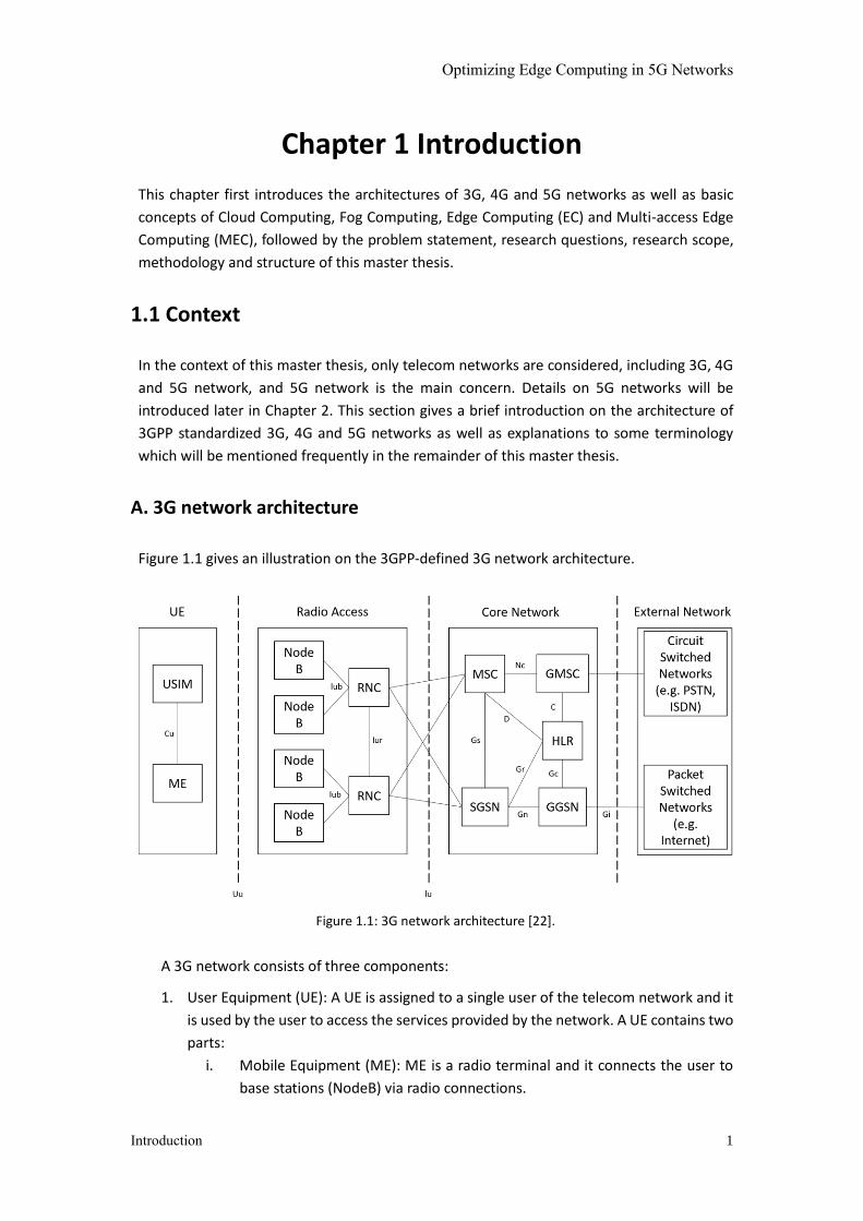
Figure 1.1 gives an illustration on the 3GPP-defined 3G network architecture.
Figure 1.1: 3G network architecture [22].
A 3G network consists of three components:
1. User Equipment (UE): A UE is assigned to a single user of the telecom network and it
is used by the user to access the services provided by the network. A UE contains two
parts:
i. Mobile Equipment (ME): ME is a radio terminal and it connects the user to
base stations (NodeB) via radio connections.
Optimizing Edge Computing in 5G Networks
Introduction 2
ii. UMTS Subscriber Identity Module (USIM): USIM is an application in the
Universal Integrated Circuit Card (UICC), and USIM is used to identify and
authenticate a subscriber on mobile telephony device (e.g. cellphone) and to
store and provide information needed by the subscriber to access the mobile
network.
2. UMTS Terrestrial Radio Access Network (UTRAN): UTRAN handles cell-level mobility.
It contains two parts:
i. Base stations (NodeB): A NodeB facilitates wireless communications between
UEs and networks. A NodeB is responsible for transmissions and receptions
of signals, encrypting and decrypting communications, amplifying and
combing signals, etc.
ii. Radio Network Controllers (RNC): An RNC is a single point of UTRAN to access
the core network and it is the aggregation point for a group of NodeBs. An
RNC controls the NodeBs that are connected to it, and it is responsible for
radio resource management, mobility management functions and user data
encryption.
3. Core network (CN): A Core network has gateways to external networks, and it is
responsible for handovers/relocations and location management. There are several
functional entities in a 3G core network and Figure 1.1 shows some of the most
important ones. Home Location Register (HLR) stores subscriber data, subscriber
state and location data of every subscriber of the relevant Public Land Mobile
Network (PLMN). A Mobile Switching Center (MSC) holds subscriber data and state.
A subscriber of the 3G network is connected to an MSC, and the MSC is responsible
for setting up and releasing end to end connections between the subscriber and
external networks. Besides this, the MSC handles mobility and call handovers. A
Gateway MSC (GMSC) is responsible for terminating call handling and it does not hold
subscriber data. A GMSC can determine which MSC a called subscriber is currently
located at and route the terminating call towards that MSC. A Serving GPRS Support
Node (SGSN) is responsible for the delivery of data packets from/towards the
subscribers within its serving area including packet routing, transfer mobility
management, authentication and charging. Gateway GPRS Supporting Node (GGSN)
is the interface between the core network and external packet-switched data
networks, and it provides connections to these external data networks.
B. 4G network architecture
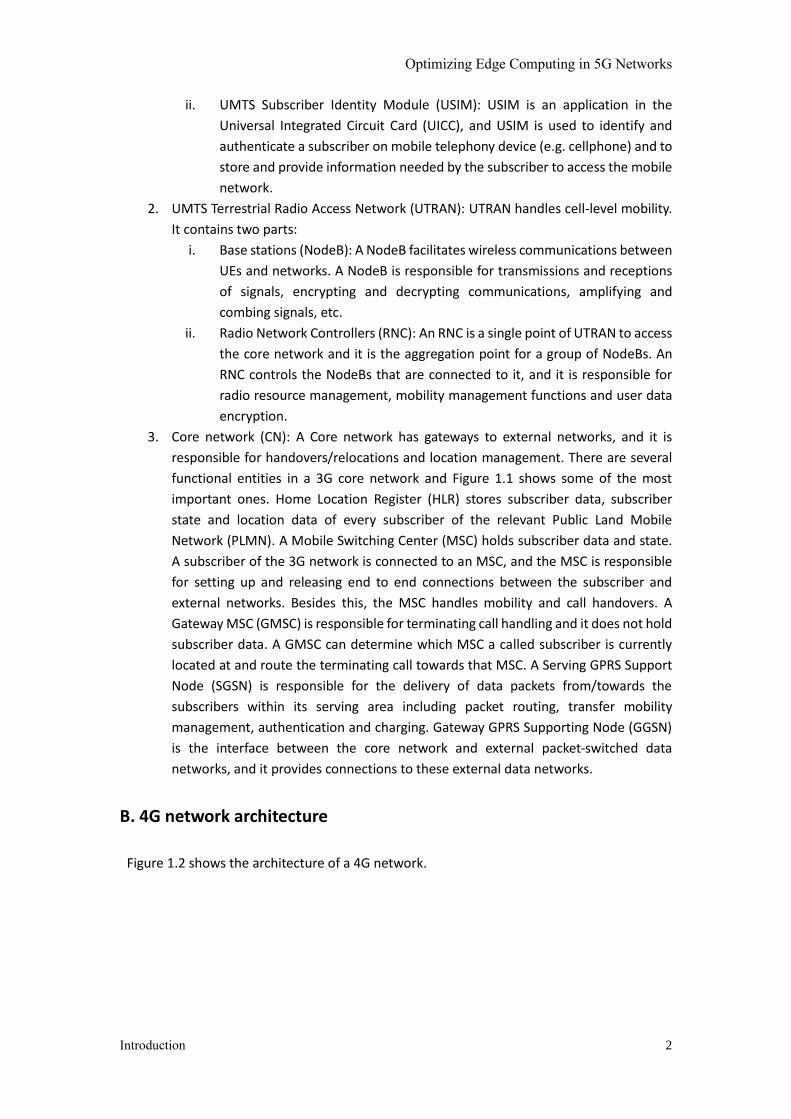
Figure 1.2 shows the architecture of a 4G network.
Optimizing Edge Computing in 5G Networks
Introduction 3
Figure 1.2: 4G network architecture [23].
A 4G network has a flat architecture in which the Evolved UMTS Terrestrial Radio Access
Network (E-UTRAN) does not contain RNCs. The eNodeBs (eNB) are base stations in a 4G
network, which connect to UEs via a radio interface E-UTRAN Uu and connect the E-UTRAN
to the Enhanced Packet Core (EPC, the core network in 4G network) via S1 interfaces.
In the EPC the Mobility Management Entity (MME) keeps track of UEs which are
registered on the LTE network. The MME is the main control element in the Enhanced Packet
Core (EPC) and it is in charge of authentication, security, mobility management, etc. A Serving
Gateway (S-Gw) serves a group of eNodeBs for user plane data and it is the local mobility
anchor for mobile UEs. In addition, a S-Gw is also responsible for setting up and tearing down
sessions for particular UEs under instructions from the MME. A Packet Data Network Gateway
(P-Gw) provides access to external data networks (e.g. Internet) and collects and reports
charging information. It is also the highest mobility anchor in the EPC. Policy and Charging
Rules Function (PCRF) provides the P-Gw with relevant charging and traffic control/routing
rules. Home Subscription Server (HSS) is the subscription data repository that storing
information like subscriber data, subscriber current location information, etc. Unlike the HLR
in the 3G network, the HSS is also responsible for subscriber authentication.
C. 5G network architecture
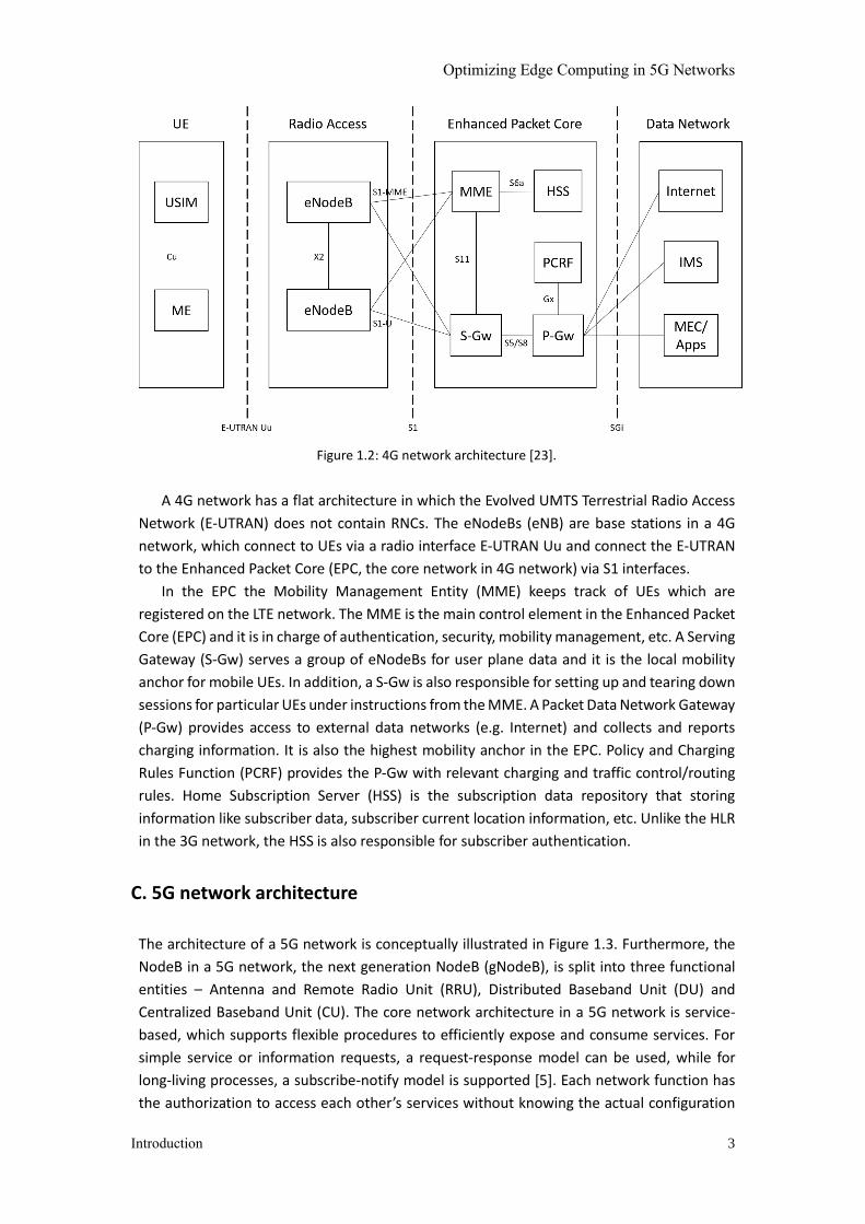
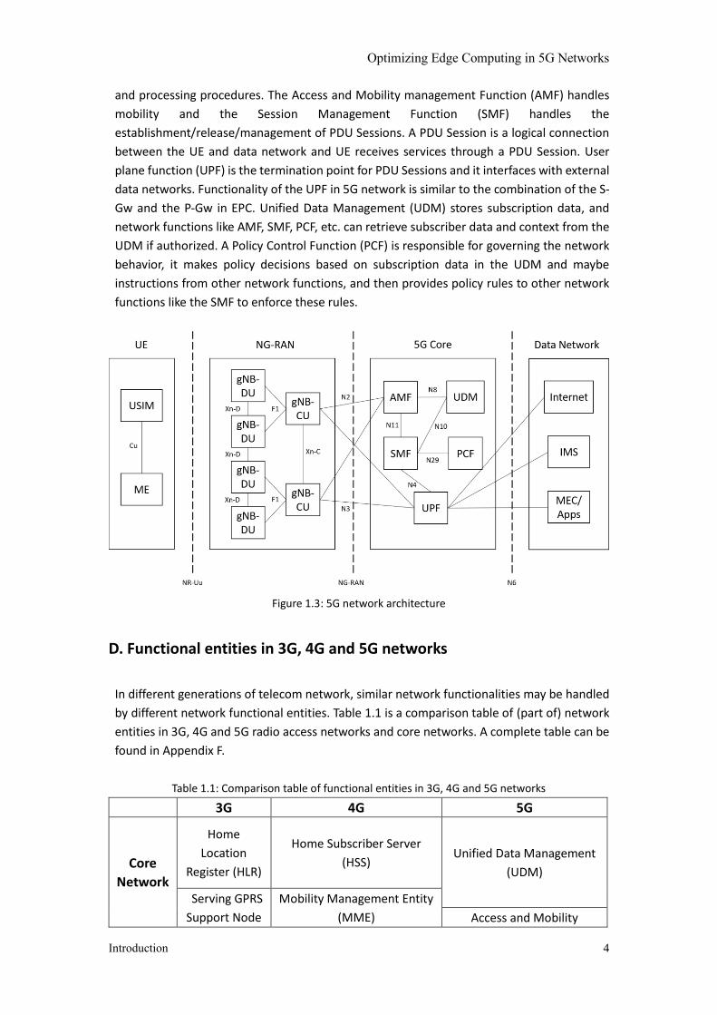
The architecture of a 5G network is conceptually illustrated in Figure 1.3. Furthermore, the
NodeB in a 5G network, the next generation NodeB (gNodeB), is split into three functional
entities – Antenna and Remote Radio Unit (RRU), Distributed Baseband Unit (DU) and
Centralized Baseband Unit (CU). The core network architecture in a 5G network is service-
based, which supports flexible procedures to efficiently expose and consume services. For
simple service or information requests, a request-response model can be used, while for
long-living processes, a subscribe-notify model is supported [5]. Each network function has
the authorization to access each other’s services without knowing the actual configuration
Optimizing Edge Computing in 5G Networks
Introduction 4
and processing procedures. The Access and Mobility management Function (AMF) handles
mobility and the Session Management Function (SMF) handles the
establishment/release/management of PDU Sessions. A PDU Session is a logical connection
between the UE and data network and UE receives services through a PDU Session. User
plane function (UPF) is the termination point for PDU Sessions and it interfaces with external
data networks. Functionality of the UPF in 5G network is similar to the combination of the S-
Gw and the P-Gw in EPC. Unified Data Management (UDM) stores subscription data, and
network functions like AMF, SMF, PCF, etc. can retrieve subscriber data and context from the
UDM if authorized. A Policy Control Function (PCF) is responsible for governing the network
behavior, it makes policy decisions based on subscription data in the UDM and maybe
instructions from other network functions, and then provides policy rules to other network
functions like the SMF to enforce these rules.
Figure 1.3: 5G network architecture
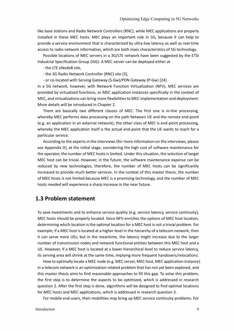
D. Functional entities in 3G, 4G and 5G networks
In different generations of telecom network, similar network functionalities may be handled
by different network functional entities. Table 1.1 is a comparison table of (part of) network
entities in 3G, 4G and 5G radio access networks and core networks. A complete table can be
found in Appendix F.
Table 1.1: Comparison table of functional entities in 3G, 4G and 5G networks
3G 4G 5G
Core
Network
Home
Location
Register (HLR)
Home Subscriber Server
(HSS) Unified Data Management
(UDM)
Serving GPRS
Support Node
Mobility Management Entity
(MME) Access and Mobility

Optimizing Edge Computing in 5G Networks
Introduction 5
(SGSN) Management Function
(AMF)
Session Management
Function (SMF)
Gateway GPRS
Support Node
(GGSN)
Serving Gateway (S-Gw)
User Plane Function (UPF)
Packet Data Network
Gateway (P-Gw) Session Management
Function (SMF)
Mobile Service
Switching
Center (MSC)
*Related to
circuit-switched
networks only
N/A N/A
Gateway MSC
(GMSC)
*Related to
circuit-switched
networks only
N/A N/A
N/A Policy and Charging Rules
Function (PCRF)
Policy Control Function
(PCF)
Radio
Access
Network
NodeB (NB)
E-UTRAN NodeB (eNB)
Next
Generation
NodeB
(gNB)
Distributed
Unit
(gNB-DU)
Radio Network
Controller
(RNC)
Centralized
Unit
(gNB-CU)
3G 4G 5G
Core
Network
Home
Location
Register (HLR)
Home Subscriber Server
(HSS) Unified Data Management
(UDM)
Serving GPRS
Support Node
(SGSN)
Mobility Management Entity
(MME)
Access and Mobility
Management Function
(AMF)

Optimizing Edge Computing in 5G Networks
Introduction 6
Session Management
Function (SMF)
Gateway GPRS
Support Node
(GGSN)
Serving Gateway (S-Gw)
User Plane Function (UPF)
Packet Data Network
Gateway (P-Gw) Session Management
Function (SMF)
Mobile service
Switching
Center (MSC)
*Related to
circuit-switched
networks only
N/A N/A
Gateway MSC
(GMSC)
*Related to
circuit-switched
networks only
N/A N/A
N/A Policy and Charging Rules
Function (PCRF)
Policy Control Function
(PCF)
Radio
Access
Network
NodeB (NB)
E-UTRAN NodeB (eNB)
Next
Generation
NodeB
(gNB)
Distributed
Unit
(gNB-DU)
Radio Network
Controller
(RNC)
Centralized
Unit
(gNB-CU)
E. Terminology
Service latency: In the context of this project, the only latency considered is the service
latency between a UE who is consuming this service and entity that is providing this service
to this UE. The service latency mainly comes from the processing time of all the network
functional elements between the UE and the serving entity as well as the processing time in
the serving entity. Therefore, if a serving entity is closer to the base station, it can guarantee
smaller service latency, since there are fewer network elements in between.
Relocation: When a mobile UE is moving, its location changes at the same time. In some
Optimizing Edge Computing in 5G Networks
Introduction 7
cases, a UE may move out of the serving area of its current serving entity (e.g. host, server,
base station, local cloud, etc.) which means that this entity can no longer provide services to
this UE anymore. To maintain the service continuity, a new entity should take over the
responsibility to serve this UE, and this process of switching from the current serving entity
to a new serving entity is called a relocation.
Logical location: The topology location where a host/server is placed is called the logical
location of this host/server. Hosts/servers in different logical locations have different
properties including service latency, since nowadays the processing time of functional
entities between the UE and the host/server is one of the major sources of service latency.
However, in the context of this thesis, a host/server is always located inside an external data
network. Therefore, logical location of every host/server is on the network side of the UPF,
and logical location is out of consideration in this master thesis.
Physical location: The actual place where a host/server is deployed in the telecom
network is called the physical location of this host/server. Today, the transmission time on
optical fibers is usually millisecond level or even lower, depending on the actual length of the
cable. Experiments and calculations show that transferring a packet from the very southern
part of the Netherlands to the very northern part of the Netherlands via optical fibers takes
only 2 milliseconds (See more in Appendix D). Despite the low transmission delay on optical
fiber, physical location is still crucial because one of the major sources of latency is the data
transformation time. If the host/server and gNodeB are located physically close to each other,
the number of transmission nodes (e.g. IP routers) in between will be reduced and the total
data transformation time will decrease at the same time. The physical location of a
host/server is one of the main concerns of this master thesis. For simplicity reason, it is
referred to as “location” in the reminder of this master thesis.
1.2 Edge Computing, Cloud Computing, Fog Computing and
Multi-access Edge Computing
In the coming 5G era, requirements on latency between the UE and the computing/storage
platform are getting more and more stringent. Since ultra-low latency has become one of the
main characteristics of 5G technology, various applications relying on low latency will appear
in the market. Traditional cloud computing may not be able to fulfill these new latency
requirements, hence, a new concept – edge computing, is now getting more and more
attention.
Optimizing Edge Computing in 5G Networks
Introduction 8
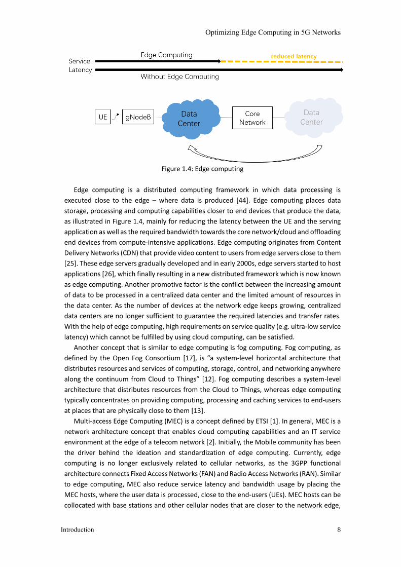
Figure 1.4: Edge computing
Edge computing is a distributed computing framework in which data processing is
executed close to the edge – where data is produced [44]. Edge computing places data
storage, processing and computing capabilities closer to end devices that produce the data,
as illustrated in Figure 1.4, mainly for reducing the latency between the UE and the serving
application as well as the required bandwidth towards the core network/cloud and offloading
end devices from compute-intensive applications. Edge computing originates from Content
Delivery Networks (CDN) that provide video content to users from edge servers close to them
[25]. These edge servers gradually developed and in early 2000s, edge servers started to host
applications [26], which finally resulting in a new distributed framework which is now known
as edge computing. Another promotive factor is the conflict between the increasing amount
of data to be processed in a centralized data center and the limited amount of resources in
the data center. As the number of devices at the network edge keeps growing, centralized
data centers are no longer sufficient to guarantee the required latencies and transfer rates.
With the help of edge computing, high requirements on service quality (e.g. ultra-low service
latency) which cannot be fulfilled by using cloud computing, can be satisfied.
Another concept that is similar to edge computing is fog computing. Fog computing, as
defined by the Open Fog Consortium [17], is “a system-level horizontal architecture that
distributes resources and services of computing, storage, control, and networking anywhere
along the continuum from Cloud to Things” [12]. Fog computing describes a system-level
architecture that distributes resources from the Cloud to Things, whereas edge computing
typically concentrates on providing computing, processing and caching services to end-users
at places that are physically close to them [13].
Multi-access Edge Computing (MEC) is a concept defined by ETSI [1]. In general, MEC is a
network architecture concept that enables cloud computing capabilities and an IT service
environment at the edge of a telecom network [2]. Initially, the Mobile community has been
the driver behind the ideation and standardization of edge computing. Currently, edge
computing is no longer exclusively related to cellular networks, as the 3GPP functional
architecture connects Fixed Access Networks (FAN) and Radio Access Networks (RAN). Similar
to edge computing, MEC also reduce service latency and bandwidth usage by placing the
MEC hosts, where the user data is processed, close to the end-users (UEs). MEC hosts can be
collocated with base stations and other cellular nodes that are closer to the network edge,
Optimizing Edge Computing in 5G Networks
Introduction 9
like base stations and Radio Network Controllers (RNC), while MEC applications are properly
installed in these MEC hosts. MEC plays an important role in 5G, because it can help to
provide a service environment that is characterized by ultra-low latency as well as real-time
access to radio network information, which are both main characteristics of 5G technology.
Possible locations of MEC servers in a 3G/LTE network have been suggested by the ETSI
Industrial Specification Group (ISG): A MEC server can be deployed either at
- the LTE eNodeB site,
- the 3G Radio Network Controller (RNC) site [3],
- or co-located with Serving Gateway (S-Gw)/PDN Gateway (P-Gw) [24].
In a 5G network, however, with Network Function Virtualization (NFV), MEC services are
provided by virtualized functions, or MEC application instances specifically in the context of
MEC, and virtualizations can bring more flexibilities to MEC implementation and deployment.
More details will be introduced in Chapter 2.
There are basically two different classes of MEC. The first one is in-line processing,
whereby MEC performs data processing on the path between UE and the remote end-point
(e.g. an application in an external network); the other class of MEC is end-point processing,
whereby the MEC application itself is the actual end-point that the UE wants to reach for a
particular service.
According to the experts in the interviews (for more information on the interviews, please
see Appendix D), at the initial stage, considering the high cost of software maintenance for
the operator, the number of MEC hosts is limited. Under this situation, the selection of target
MEC host can be trivial. However, in the future, the software maintenance expense can be
reduced by new technologies, therefore, the number of MEC hosts can be significantly
increased to provide much better services. In the context of this master thesis, the number
of MEC hosts is not limited because MEC is a promising technology, and the number of MEC
hosts needed will experience a sharp increase in the near future.
1.3 Problem statement
To save investments and to enhance service quality (e.g. service latency, service continuity),
MEC hosts should be properly located. Since NFV enriches the options of MEC host location,
determining which location is the optimal location for a MEC host is not a trivial problem. For
example, if a MEC host is located at a higher level in the hierarchy of a telecom network, then
it can serve more UEs; but in the meantime, the latency might increase due to the larger
number of transmission nodes and network functional entities between this MEC host and a
UE. However, if a MEC host is located at a lower-hierarchical level to reduce service latency,
its serving area will shrink at the same time, implying more frequent handovers/relocations.
How to optimally locate a MEC node (e.g. MEC server, MEC host, MEC application instance)
in a telecom network is an optimization-related problem that has not yet been explored, and
this master thesis aims to find reasonable approaches to fill this gap. To solve this problem,
the first step is to determine the aspects to be optimized, which is addressed in research
question 2. After the first step is done, algorithms will be designed to find optimal locations
for MEC hosts and MEC applications, which is addressed in research question 3.
For mobile end-users, their mobilities may bring up MEC service continuity problems. For
Optimizing Edge Computing in 5G Networks
Introduction 10
example, if one self-driving vehicle is moving on the road, receiving MEC services from its
current MEC host 𝐴 , and it may move out of the serving area of 𝐴 after some time. To
maintain the MEC services of this vehicle, another MEC host 𝐵 should take over the
responsibility for serving this vehicle. To achieve this, a relocation is needed to transfer user
context from MEC host 𝐴 to MEC host 𝐵, and MEC host 𝐵 is called the target MEC host of
this relocation. In a telecom network, there may exist multiple MEC hosts that can be the
target MEC host of a relocation. Therefore, it is necessary to determine which MEC host is
the most suitable one.
How to find the optimal target MEC host of a relocation is an optimization problem that
has not yet been explored, and it is another research gap that this master thesis focuses on.
Algorithms will be designed to decide on the optimal target MEC host of a relocation, which
is addressed in research question 4.
1.4 Research questions
There are 4 research questions in this master thesis project:
1. What is Edge Computing and what is the relevance of different types of computing
for telecom operators?
2. What aspects of Edge Computing should be considered for optimization in the
context of 5G?
3. Devise an algorithm to find the optimal location of MEC hosts and the optimal
location (MEC host) of a MEC application.
To solve this, the following sub-questions are identified:
a) Determine which aspects of MEC applications need to be considered in this
master thesis.
b) Transform the aspects chosen in sub-question a) into a set of parameters.
c) Locate the MEC hosts as well as MEC applications properly based on these
parameters.
d) How to test the performance of the algorithm?
4. Devise an algorithm to dynamically find the optimal location of a MEC application
processing instance for a UE (can be all kinds of equipment mounted in vehicles,
machines, cellphones, etc.).
To solve this, the following sub-questions are identified:
a) What parameters of the possible target MEC hosts should be taken into
consideration?
b) How to choose the target MEC host based on these parameters?
c) What information can be provided as feedback after a relocation to estimate
the quality of this relocation and the behavior of the target MEC host? How to
process/utilize the feedback information?
d) How to test the performance of the algorithm?

Optimizing Edge Computing in 5G Networks
Introduction 11
1.5 Research Scope
In this master thesis, the considered MEC application users can be categorized into two
categories which are described below:
1. Vehicle-to-everything (V2X) communications for self-driving vehicles. This type of UEs
have high requirements on the application instance/UE context mobility service and
the relocation mechanism.
Theoretically, a large vehicle might be able to run and hold a MEC host itself and
possibly has the ability to do the relevant signaling and data processing for other
vehicles in its vicinity. Although using these vehicles to serve other MEC service users
might significantly reduce the service latency, the high mobility of the MEC host
located inside this serving vehicle may result in other problems. For instance, for a
vehicle that moves at a similar speed as the serving vehicle, connecting to this serving
vehicle can be a good way to reduce the number of relocations, while for the other
vehicles, connecting to this moving MEC host may result in more relocations.
Therefore, considering these vehicles as potential MEC hosts to serve UEs will
significantly increase the complexity of this master thesis, hence, in this thesis all the
MEC hosts considered are stationary MEC hosts whose locations are fixed.
2. Data caching and instant data processing for end-users on moving devices. One typical
example is an end-user on a high-speed vehicle watching on-line videos or playing
video games using a cellphone. For these kinds of applications/services, MEC is also
important due to their requirements on instant interactions between the UEs, real-
time user data processing and the fluent, high quality data stream between the UE
and the server that provides the video stream. Compared to self-driving vehicles, the
MEC service continuity for end-users in this category is less crucial, therefore, their
mobility requirements can be less stringent.
Security and privacy aspects will not be considered in this master thesis. The 3GPP-defined
5G architecture itself contains several security-related designs already. For example, if the
MEC platform/MEC orchestrator, working as an Application Function (AF), is not trusted and
authorized, it will not directly interact with the Policy Control Function (PCF) but
communicate with the Network Exposure Function (NEF) instead.
1.6 Methodology
Literature review and paper study are used throughout the entire master thesis. Research
questions 1 and 2 especially rely on literature review since reading standardizations and
white papers can help understand the meaning of relevant terminology as well as the basic
ideas and usages of edge computing and MEC. Apart from that, greedy algorithms, heuristic
algorithms, Markov Decision Process (MDP) and Reinforcement Learning (RL) are used to
solve research questions 3 and 4, which will be further introduced in chapters 3, 4 and 5.
Optimizing Edge Computing in 5G Networks
Introduction 12
1.7 Structure of the thesis
Chapter 2 introduces some basic knowledge about 5G networks, MEC and MEC deployment
in 5G networks. In Chapter 2 the research questions 1 and 2 are answered. Chapter 3 solves
research question 3 and its sub-questions, introduces the details and technology background
of all the designed algorithms, and shows, compares and analyzes the performance of these
algorithms. Chapter 4 solves research question 4 and its sub-questions and introduces the
details and technology background of all the designed algorithms. Chapter 5 gives the
background introduction on the +31 Network in Ericsson, Rijen and shows the measurement
results measured from the +31 Network. In Chapter 5, the performance of the algorithms
designed in Chapter 4 are tested via simulations and the simulation tools and settings are
introduced. Simulation outcomes are shown, compared and analyzed. Chapter 6 gives the
overall conclusions of this master thesis and recommendations for potential future related
work.

Optimizing Edge Computing in 5G Networks
Multi-access Edge Computing in the context of 5G 13
Chapter 2 Multi-access Edge Computing in
the context of 5G
In this chapter, background information on 5G network is provided, including 5G network
architecture, network functional entities and reference points. Apart from that, MEC system
architecture, MEC entities and reference points are introduced, followed by the knowledge
of MEC deployment in a 5G network, MEC-related UE mobility management and MEC
lifecycle management.
2.1 5G network architecture
A 5G system, according to 3GPP standardization, consists of a 5G network and 5G User
Equipment (UE) [4], and a 5G network contains a 5G Access Network (5G AN) and a 5G Core
Network (5GC). A 5G AN is an access network comprising a Next Generation Radio Access
Network (NG-RAN) and/or a non-3GPP Access Network (AN) connecting to a 5GC [4]. A NG-
RAN consists of base stations, which are called Next Generation NodeB (gNodeB, or gNB) and
Next Generation E-UTRAN NodeB (ng-eNB).
Specified by 3GPP in [4], the 5G network architecture is shown in Figure 2.1, and Figure
2.2 depicts the 3GPP [16] architecture of a 5G RAN.
At the highest system level, the 3GPP architecture contains 10 different Network
Functions (NF). A network function can be realized in:
- a network element on dedicated hardware,
- an application instance running on dedicated hardware or
- a virtualized network function instantiated on an appropriate platform [4].
5G network architecture is a Service-Based Architecture (SBA), where a network function can
provide services to other network functions or consume services other network functions
provide. In this way, network functions communicate with each other, and the inner workings
of one network function is a black box to the others. All the available services are registered
in the Network Repository Function (NRF); if an authorized function needs to use a certain
service, it can directly interact with the service provider, another network function, or gain
the access towards the service via the Network Exposure Function (NEF).
However, untrusted entities, mainly located outside the 5G core network, cannot access
the services by interacting with network functions directly. Instead, external, untrusted
entities access services provided in 5GC via the NEF.
AMF, or Access and Mobility management Function, is responsible for registration
management, connection management, reachability management, mobility management,
access management, authorization and security-related management [4]. Besides, AMF also
allows subscriptions of notifications regarding mobility events [5].
SMF is the Session Management Function. As mentioned in its name, SMF is responsible
for Protocol Data Unit (PDU) Session (PDU Session) establishment, modification and release.
Unified Data Management Function (UDM) is for storing and managing subscription and

Optimizing Edge Computing in 5G Networks
Multi-access Edge Computing in the context of 5G 14
user data. Authentication Server Function (AUSF) is used for authentication.
Network Exposure Function (NEF) is a centralized service exposure point, and it is
responsible for authorizing access requests from outside the network.
Policy Control Function (PCF) handles policies and rules by interacting with subscription
data and user context provided by the UDM as well as instructions from Network Exposure
Function (NEF) and/or Application Functions (AF).
Network Slice Selection Function (NSSF) helps the UE in the network with finding proper
network slice instance, and according to the slides that the UE has access to, an AMF is
selected to serve the UE, which may be different from the one that is previously selected by
the access network to receive the registration request from the UE. If the newly selected AMF
is different from the old one, the UE will be handed off to the new AMF.
A User Plane Function (UPF) is the end-point of the PDU Session and forms the gateway
to data networks. It plays an important role in MEC since it relies on UPFs to route the desired
traffic towards the MEC applications. Both the MEC Orchestrator (MEO) at superior system
level and the MEC platform on the host level can act as an Application Function (AF) and
interfere the traffic steering rules configuration. If the AF is authorized, it will directly
communicate with the PCF to manipulate traffic rules configuration; otherwise the AF will
interact with the NEF, and the NEF will instruct the PCF to create rules based on the
requirements from MEO. The PCF will then send the traffic rules to the relevant SMF and the
SMF will instruct the UPF to do traffic steering accordingly.
Figure 2.1: 3GPP 5G service-based architecture [4].
gNB
ng-eNB
NG
NG
NG
Xn
NG-RAN
5GC
AMF/UPF
gNB
ng-eNB
NG
NG
NG
Xn
AMF/UPF
Xn
Xn
NG NG
Figure 2.2: Overall NG-RAN architecture [28].

Optimizing Edge Computing in 5G Networks
Multi-access Edge Computing in the context of 5G 15
Figure 2.2 shows two types of NG-RAN nodes: Next Generation NodeB (gNB) and Next
Generation E-UTRAN NodeB (ng-eNB). The gNB provides the New Radio (NR) user plane and
control plane protocol terminations towards the UE, while the ng-eNB provides the Evolved
UMTS Terrestrial Radio Access (E-UTRA) user plane and control plane protocol terminations
towards the UE. The gNBs and ng-eNBs are responsible for radio resource management (e.g.
radio bearer control, radio admission control, connection mobility control, dynamic
allocation of resources to UEs in both uplink and downlink), routing User Plane (UP) data
towards UPF(s) and Control Plane (CP) data towards AMF, connection setup and release,
measurement and measurement reporting configuration for mobility and scheduling, QoS
flow management, etc.
Figure 2.3: Overall architecture of a gNB.
The concept shown in Figure 2.3 is the separation of the control plane and the user plane
inside a gNodeB. A Next Generation NodeB Centralized Unit Control Plane (gNB-CU-CP) can
control one or more Next Generation NodeB Centralized Unit User Planes (gNB-CU-UP). A
gNB-DU can be controlled by only one gNB-CU-CP but can connect to one or more gNB-CU-
UPs. With network virtualization, gNB-CU-UPs can be located anywhere with required
hardware resources available, for example, a gNB-CU-CP can be located physically close to a
gNB-DU or an UPF.
Normally, which gNB-CU-CP controls which gNB-DUs is determined by the telecom
operator. When a UE wants to establish a PDU Session, it will first send a request to the gNB-
DU which it is connected to, and this gNB-DU will send another request to its corresponding
gNB-CU-CP, then the gNB-CU-CP will find a suitable gNB-CU-UP to set up the bearer context.
Optimizing Edge Computing in 5G Networks
Multi-access Edge Computing in the context of 5G 16
2.2 MEC system architecture
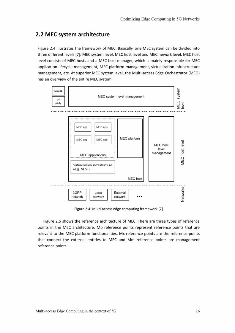
Figure 2.4 illustrates the framework of MEC. Basically, one MEC system can be divided into
three different levels [7]: MEC system level, MEC host level and MEC nework level. MEC host
level consists of MEC hosts and a MEC host manager, which is mainly responsible for MEC
application lifecycle management, MEC platform management, virtualization infrastructure
management, etc. At superior MEC system level, the Multi-access Edge Orchestrator (MEO)
has an overview of the entire MEC system.
Figure 2.4: Multi-access edge computing framework [7]
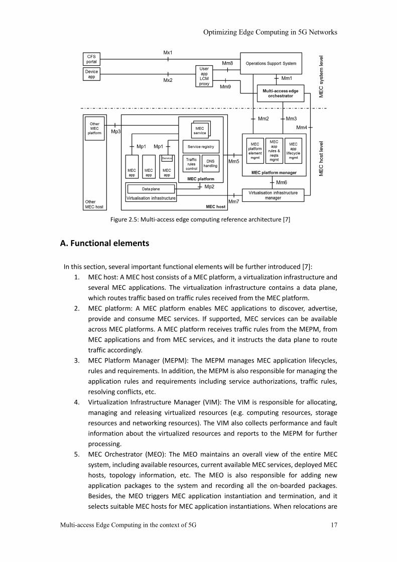
Figure 2.5 shows the reference architecture of MEC. There are three types of reference
points in the MEC architecture: Mp reference points represent reference points that are
relevant to the MEC platform functionalities, Mx reference points are the reference points
that connect the external entities to MEC and Mm reference points are management
reference points.
Optimizing Edge Computing in 5G Networks
Multi-access Edge Computing in the context of 5G 17
Figure 2.5: Multi-access edge computing reference architecture [7]
A. Functional elements
In this section, several important functional elements will be further introduced [7]:
1. MEC host: A MEC host consists of a MEC platform, a virtualization infrastructure and
several MEC applications. The virtualization infrastructure contains a data plane,
which routes traffic based on traffic rules received from the MEC platform.
2. MEC platform: A MEC platform enables MEC applications to discover, advertise,
provide and consume MEC services. If supported, MEC services can be available
across MEC platforms. A MEC platform receives traffic rules from the MEPM, from
MEC applications and from MEC services, and it instructs the data plane to route
traffic accordingly.
3. MEC Platform Manager (MEPM): The MEPM manages MEC application lifecycles,
rules and requirements. In addition, the MEPM is also responsible for managing the
application rules and requirements including service authorizations, traffic rules,
resolving conflicts, etc.
4. Virtualization Infrastructure Manager (VIM): The VIM is responsible for allocating,
managing and releasing virtualized resources (e.g. computing resources, storage
resources and networking resources). The VIM also collects performance and fault
information about the virtualized resources and reports to the MEPM for further
processing.
5. MEC Orchestrator (MEO): The MEO maintains an overall view of the entire MEC
system, including available resources, current available MEC services, deployed MEC
hosts, topology information, etc. The MEO is also responsible for adding new
application packages to the system and recording all the on-boarded packages.
Besides, the MEO triggers MEC application instantiation and termination, and it
selects suitable MEC hosts for MEC application instantiations. When relocations are
Optimizing Edge Computing in 5G Networks
Multi-access Edge Computing in the context of 5G 18
supported, the MEO will trigger relocations if needed.
6. Operations Support System (OSS): The OSS receives MEC application instantiation
and termination requests from external parties and UE applications, and decides on
the granting of these requests. The granted requests are forwarded to MEO for
further processing.
7. Customer Facing Service portal (CFS portal): A CFS portal is used by third-party
customers of operators for selecting and ordering a set of MEC applications they
need and for receiving further service-level information.
B. Reference points
Reference points define conceptual points of information exchange between non-
overlapping functional entities. A reference point becomes an interface when the connected
functional entities are embodied in separate pieces of equipment [27]. In this section, the
main reference points will be introduced in more details, information on reference points
which are not mentioned below, so far as MEC is concerned, can be found in [7]:
1. Mx2: This reference point connects the MEC system and external UEs. UEs can use
this reference point to request the MEC system to run a MEC application, or to move
MEC applications in/out of the MEC system.
2. Mp1: This reference point connects a MEC application and the MEC platform. Mp1
is used by a MEC application to provide or consume other MEC services.
3. Mp2: This reference point connects the data plane and the MEC platform. MEC
platform uses it to provide the data plane with traffic routing rules.
4. Mp3: This reference point connects two different MEC platforms, and these two MEC
platforms can belong to different MEC systems if supported. Connecting two MEC
platforms in two different MEC systems via Mp3 can facilitate coordination between
MEC systems.
5. Mm1: This reference point connects the OSS and the MEO. Mm1 is mainly used for
triggering the instantiation and termination of MEC applications.
6. Mm3: This reference point connects the MEO and the MEPM. Mm3 is used to
perform MEC application lifecycle management (LCM), MEC application rules &
requirements management and MEC services tracking.
7. Mm4: This reference point connects the MEO and the VIM. Mm4 is used to track
available resources, manage application images and other virtualized resources
related management.
8. Mm6: This reference point connects the MEPM and the VIM. Mm6 is used to manage
virtualized resources in the MEC system.
9. Mm8: This reference point connects a User Application LCM Proxy (UALCMP) and the
OSS. Mm8 is used to handle requests of running MEC applications in the MEC system
from external UE applications (device applications).
10. Mm9: This reference point connects a UALCMP and the MEO. Unlike reference point
Mm8, Mm9 is used for managing MEC applications which are requested by UE
applications (device applications).
Optimizing Edge Computing in 5G Networks
Multi-access Edge Computing in the context of 5G 19
2.3 MEC system deployed in 5G network
A. Overall Introduction
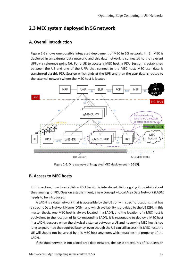
Figure 2.6 shows one possible integrated deployment of MEC in 5G network. In [5], MEC is
deployed in an external data network, and this data network is connected to the relevant
UPFs via reference point N6. For a UE to access a MEC host, a PDU Session is established
between the UE and one of the UPFs that connect to the MEC host. MEC user data is
transferred via this PDU Session which ends at the UPF, and then the user data is routed to
the external network where the MEC host is located.
Figure 2.6: One example of integrated MEC deployment in 5G [5].
B. Access to MEC hosts
In this section, how to establish a PDU Session is introduced. Before going into details about
the signaling for PDU Session establishment, a new concept – Local Area Data Network (LADN)
needs to be introduced.
A LADN is a data network that is accessible by the UEs only in specific locations, that has
a specific Data Network Name (DNN), and which availability is provided to the UE [29]. In this
master thesis, one MEC host is always located in a LADN, and the location of a MEC host is
equivalent to the location of its corresponding LADN. It is reasonable to deploy a MEC host
in a LADN, because when the physical distance between a UE and its serving MEC host is too
long to guarantee the required latency, even though the UE can still access this MEC host, the
UE will should not be served by this MEC host anymore, which matches the property of the
LADN.
If the data network is not a local area data network, the basic procedures of PDU Session
Optimizing Edge Computing in 5G Networks
Multi-access Edge Computing in the context of 5G 20
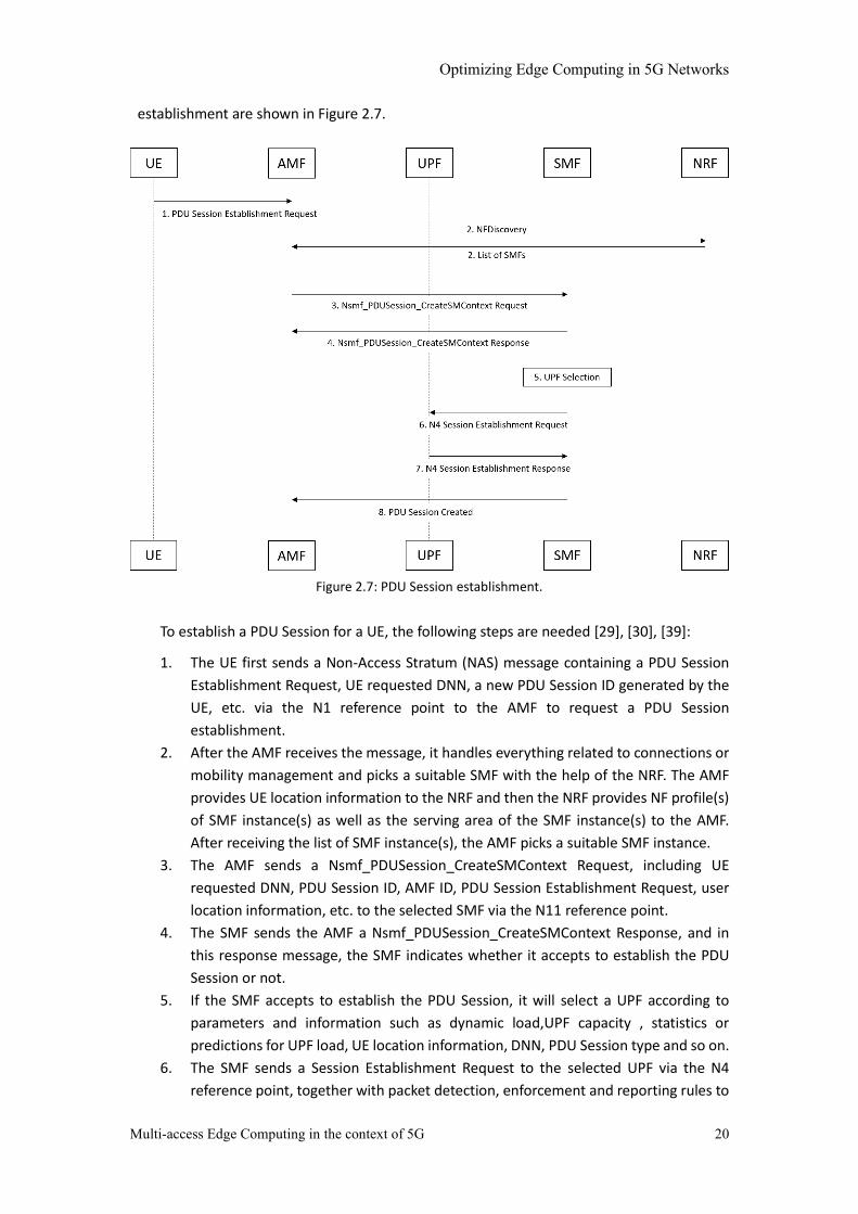
establishment are shown in Figure 2.7.
Figure 2.7: PDU Session establishment.
To establish a PDU Session for a UE, the following steps are needed [29], [30], [39]:
1. The UE first sends a Non-Access Stratum (NAS) message containing a PDU Session
Establishment Request, UE requested DNN, a new PDU Session ID generated by the
UE, etc. via the N1 reference point to the AMF to request a PDU Session
establishment.
2. After the AMF receives the message, it handles everything related to connections or
mobility management and picks a suitable SMF with the help of the NRF. The AMF
provides UE location information to the NRF and then the NRF provides NF profile(s)
of SMF instance(s) as well as the serving area of the SMF instance(s) to the AMF.
After receiving the list of SMF instance(s), the AMF picks a suitable SMF instance.
3. The AMF sends a Nsmf_PDUSession_CreateSMContext Request, including UE
requested DNN, PDU Session ID, AMF ID, PDU Session Establishment Request, user
location information, etc. to the selected SMF via the N11 reference point.
4. The SMF sends the AMF a Nsmf_PDUSession_CreateSMContext Response, and in
this response message, the SMF indicates whether it accepts to establish the PDU
Session or not.
5. If the SMF accepts to establish the PDU Session, it will select a UPF according to
parameters and information such as dynamic load,UPF capacity , statistics or
predictions for UPF load, UE location information, DNN, PDU Session type and so on.
6. The SMF sends a Session Establishment Request to the selected UPF via the N4
reference point, together with packet detection, enforcement and reporting rules to
Optimizing Edge Computing in 5G Networks
Multi-access Edge Computing in the context of 5G 21
be installed on the UPF for this PDU Session.
7. The selected UPF acknowledges the request by sending a Session Establishment
Response to the SMF via the N4 reference point.
8. The SMF reports to the AMF for the successful session establishment.
If the data network is a local area data network, a few more steps are needed [29].
1. The UE provides LADN Information (i.e. LADN Service Area Information and LADN
DNN) to the AMF.
2. When receiving a PDU Session establishment request with the UE requested DNN,
the AMF determines whether the requested DNN is configured as a LADN DNN or
not. If the requested DNN points to a LADN, the AMF determines the UE’s presence
in the requested LADN service area and forwards the result to the SMF.
3. When receiving the session management request corresponding to a LADN, the SMF
determines whether the UE is inside the LADN service area based on the indication
(i.e. UE Presence in LADN service area) received. If the SMF does not receive the
indication, the SMF will consider the UE to be outside the LADN service area, and the
SMF shall then reject the PDU Session establishment request.
C. Possible Locations of MEC hosts
At the current stage, implementing and maintaining MEC hosts are expensive. Therefore, the
total number of MEC hosts is small, in order to limit the Operations and Management (O&M)
expenses from the telecom operators’ side (See more in Appendix D Interview 2). In this case,
optimizing MEC application and MEC host deployments as well as MEC host re-selections is
trivial. However, in the near future, technological advances such as network virtualization
are expected to contribute to reducing O&M cost for telecom operators. By then, locations
of UPFs are not limited to the core network anymore. Instead, UPFs can be virtualized and be
placed at more locations in the telecom network, for example, close to gNB-CUs or gNB-DUs.
If a MEC host is located further away from the network edge, the service latency will increase,
but the serving area of this MEC host will expand at the same time, implying a decrease in
the number of relocations experienced by UEs. This trade-off between service latency and
number of relocations makes optimizing the deployment of MEC hosts and MEC applications
as well as optimizing MEC host re-selection procedure non-trivial and this topic is further
discussed in this master thesis.
Optimizing Edge Computing in 5G Networks
Multi-access Edge Computing in the context of 5G 22
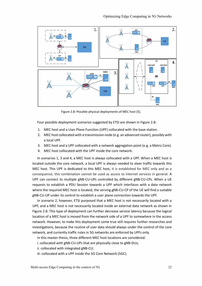
Figure 2.8: Possible physical deployments of MEC host [5].
Four possible deployment scenarios suggested by ETSI are shown in Figure 2.8:
1. MEC host and a User Plane Function (UPF) collocated with the base station.
2. MEC host collocated with a transmission node (e.g. an advanced router), possibly with
a local UPF.
3. MEC host and a UPF collocated with a network aggregation point (e.g. a Metro Core).
4. MEC host collocated with the UPF inside the core network.
In scenarios 1, 3 and 4, a MEC host is always collocated with a UPF. When a MEC host is
located outside the core network, a local UPF is always needed to steer traffic towards this
MEC host. This UPF is dedicated to this MEC host, it is established for MEC only and as a
consequence, this combination cannot be used as access to internet services in general. A
UPF can connect to multiple gNB-CU-UPs controlled by different gNB-CU-CPs. When a UE
requests to establish a PDU Session towards a UPF which interfaces with a data network
where the required MEC host is located, the serving gNB-CU-CP of the UE will find a suitable
gNB-CU-UP under its control to establish a user plane connection towards the UPF.
In scenario 2, however, ETSI purposed that a MEC host is not necessarily located with a
UPF, and a MEC host is not necessarily located inside an external data network as shown in
Figure 2.8. This type of deployment can further decrease service latency because the logical
location of a MEC host is moved from the network side of a UPF to somewhere in the access
network. However, to make this deployment come true still requires further researches and
investigations, because the routine of user data should always under the control of the core
network, and currently traffic rules in 5G networks are enforced by UPFs only.
In this master thesis, three different MEC host locations are considered:
i. collocated with gNB-CU-UPs that are physically close to gNB-DUs;
ii. collocated with integrated gNB-CU;
iii. collocated with a UPF inside the 5G Core Network (5GC).
Optimizing Edge Computing in 5G Networks
Multi-access Edge Computing in the context of 5G 23
D. Traffic Steering
The 5G network allows external AFs to provide traffic steering rules via the PCF or the NEF.
For example, MEC Functional Elements (FE) can be considered as AFs and can manipulate
traffic steering in the following ways:
1. If the MEC FE (e.g. MEP) is considered trusted by the 5G core network, this MEC FE
can directly interact with the PCF for traffic steering. The MEC FE first sends a request
to the PCF, identifying the traffic to be steered to the MEC system. Then the PCF
transforms the request into policies and provides traffic routing rules to the SMF.
Upon the arrival of the new traffic rules, the SMF will try to identify the target UPF
and start traffic rules configuration.
2. If the MEC FE is not trusted by the 5G Core Network (CN), then it needs to configure
desired traffic rules via the NEF.
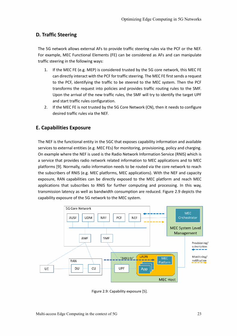
E. Capabilities Exposure
The NEF is the functional entity in the 5GC that exposes capability information and available
services to external entities (e.g. MEC FEs) for monitoring, provisioning, policy and charging.
On example where the NEF is used is the Radio Network Information Service (RNIS) which is
a service that provides radio network related information to MEC applications and to MEC
platforms [9]. Normally, radio information needs to be routed via the core network to reach
the subscribers of RNIS (e.g. MEC platforms, MEC applications). With the NEF and capacity
exposure, RAN capabilities can be directly exposed to the MEC platform and reach MEC
applications that subscribes to RNIS for further computing and processing. In this way,
transmission latency as well as bandwidth consumption are reduced. Figure 2.9 depicts the
capability exposure of the 5G network to the MEC system.
Figure 2.9: Capability exposure [5].
Optimizing Edge Computing in 5G Networks
Multi-access Edge Computing in the context of 5G 24
2.4 MEC application instance and/or UE context mobility
UEs installed in vehicles and cellphones are expected to be predominantly mobile. When a
UE is moving around, its serving site (i.e. antenna & RRU) keeps changing for maintaining a
continuous radio connection. When the serving site of a UE changes, its serving MEC host
may remain the same, thus no relocation is needed. Only when the UE moves out of the
serving area of its current serving MEC host or the change of site results in the change of UPF,
will a relocation be required in order to continue the MEC services.
According to [20], two different types of MEC applications need to be considered:
1. Dedicated MEC application: A MEC application instance is dedicated to a specific UE.
When a UE moves to a new MEC host which is different from its current serving MEC
host, its corresponding MEC application instance should be relocated to the new
MEC host from its current serving MEC host.
2. Shared MEC application: A MEC application instance serves multiple UEs. When a UE
moves to a new MEC host which is different from its current serving MEC host, if the
required MEC application has already been instantiated, then no new MEC
application instance will be instantiated.
Shared MEC applications can be further divided into two different types:
i. Stateless MEC application: A stateless application is an application that
does not memorize the service state or recorded data about UE for use in
the next service session.
ii. Stateful MEC application: An application that can record and store the state
information which can be used to facilitate service continuity during the
session transition.
Especially for stateful MEC applications and dedicated MEC applications, the
synchronization between the source and target MEC application instance as well as the user
context transfer are of great importance. After a relocation is triggered, the user context
should be copied to the target MEC application instance, after which the target MEC host is
ready to serve the UE. In order to provide seamless services, the target MEC host should be
ready when the UE moves out of the serving area of its current MEC host. Otherwise, the
target MEC host needs to act as a replay point and forward user data towards the source MEC
host for processing. In this scenario, user data transfer between the two MEC hosts increases
service latency significantly. Therefore, this scenario is not suitable for UEs with stringent
service latency requirement.
The research on MEC application mobility by ETSI MEC ISG is on-going. Up to now, several
possible procedures have been defined, including application mobility enablement, detection
of User Equipment (UE) movement, validation of application mobility, user context transfer
and/or application instance relocation, and post-processing of application relocation [5].
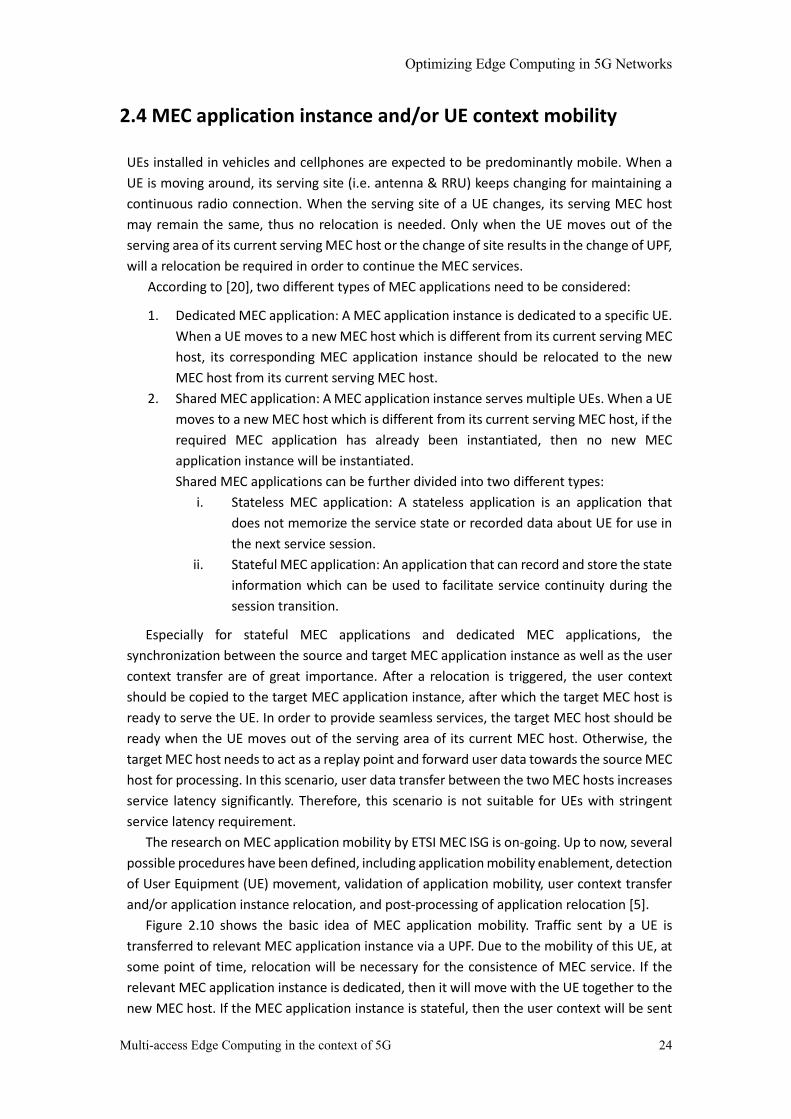
Figure 2.10 shows the basic idea of MEC application mobility. Traffic sent by a UE is
transferred to relevant MEC application instance via a UPF. Due to the mobility of this UE, at
some point of time, relocation will be necessary for the consistence of MEC service. If the
relevant MEC application instance is dedicated, then it will move with the UE together to the
new MEC host. If the MEC application instance is stateful, then the user context will be sent
Optimizing Edge Computing in 5G Networks
Multi-access Edge Computing in the context of 5G 25
to the new MEC host during a relocation.
Figure 2.10: The principle of MEC application mobility [5].
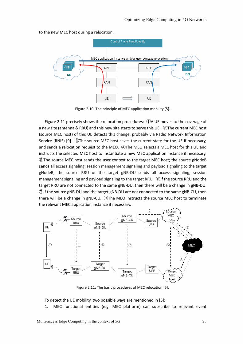
Figure 2.11 precisely shows the relocation procedures: ①A UE moves to the coverage of
a new site (antenna & RRU) and this new site starts to serve this UE. ②The current MEC host
(source MEC host) of this UE detects this change, probably via Radio Network Information
Service (RNIS) [9]. ③The source MEC host saves the current state for the UE if necessary,
and sends a relocation request to the MEO. ④The MEO selects a MEC host for this UE and
instructs the selected MEC host to instantiate a new MEC application instance if necessary.
⑤The source MEC host sends the user context to the target MEC host; the source gNodeB
sends all access signaling, session management signaling and payload signaling to the target
gNodeB; the source RRU or the target gNB-DU sends all access signaling, session
management signaling and payload signaling to the target RRU. ⑥If the source RRU and the
target RRU are not connected to the same gNB-DU, then there will be a change in gNB-DU.
⑦If the source gNB-DU and the target gNB-DU are not connected to the same gNB-CU, then
there will be a change in gNB-CU. ⑧The MEO instructs the source MEC host to terminate
the relevant MEC application instance if necessary.
Figure 2.11: The basic procedures of MEC relocation [5].
To detect the UE mobility, two possible ways are mentioned in [5]:
1. MEC functional entities (e.g. MEC platform) can subscribe to relevant event
Optimizing Edge Computing in 5G Networks
Multi-access Edge Computing in the context of 5G 26
notifications provided by the Session Management Function (SMF) or the Network
Exposure Function (NEF).
2. MEC platform can subscribe to the Radio Network Information provided by Radio
Network Information Service (RNIS). By doing this, the MEC platform can notice the
mobility of the UE when its serving cell changes.
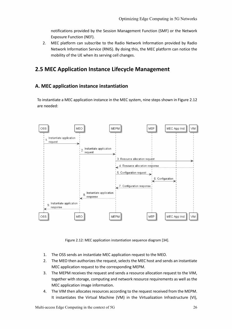
2.5 MEC Application Instance Lifecycle Management
A. MEC application instance instantiation
To instantiate a MEC application instance in the MEC system, nine steps shown in Figure 2.12
are needed:
Figure 2.12: MEC application instantiation sequence diagram [34].
1. The OSS sends an instantiate MEC application request to the MEO.
2. The MEO then authorizes the request, selects the MEC host and sends an instantiate
MEC application request to the corresponding MEPM.
3. The MEPM receives the request and sends a resource allocation request to the VIM,
together with storage, computing and network resource requirements as well as the
MEC application image information.
4. The VIM then allocates resources according to the request received from the MEPM.
It instantiates the Virtual Machine (VM) in the Virtualization Infrastructure (VI),
Optimizing Edge Computing in 5G Networks
Multi-access Edge Computing in the context of 5G 27
installs the MEC application on the VM and runs the VM as well as the application
instance.
5. The MEPM sends a configuration request to the MEC Platform (MEP). Then start the
MEC application start-up procedure.
6. In the start-up procedure, the MEC platform can verify the authenticity of the MEC
application by using an AA entity that contains the registration related information
about the MEC application [38]. Then the MEC application sends a “MEC App is
running” message to the MEP to indicate the success of the instantiation. By then
the start-up procedure is completed, and the MEC application instance will send a
service query and/or send a service registration request to the MEP to consume the
MEC applications it requests and/or register the services it provides.
7. After all the configurations in step 6 are completed, the MEP sends a configuration
response to the MEPM.
8. After the MEPM receives the configuration response, it sends an instantiate MEC
application response to the MEO, including the information of the allocated
resources for the MEC application instance.
9. The MEO sends an instantiate application response to the OSS, including the results
of this instantiation operation. If the MEC application is instantiated successfully, the
MEO will also return the corresponding application instance ID to the OSS.
B. MEC application instance termination
The procedure to terminate a MEC application instance is shown in Figure 2.13.

Optimizing Edge Computing in 5G Networks
Multi-access Edge Computing in the context of 5G 28
Figure 2.13: MEC application instance termination sequence diagram [34].
1. The OSS sends a terminate application instance request to the MEO, together with
the MEC application instance ID of the application instance to be terminated.
2. The MEO authorizes the request and verifies the existence of the identified
application instance. The MEO then sends a terminate application instance request
to the MEPM.
3. The MEPM sends the terminate application instance request to the relevant MEP.
4. The MEP receives the terminate application instance request from the MEPM. If a
graceful termination is requested and is supported by the MEC application to be
terminated, then the MEP starts the graceful stop procedure: The MEP first sends an
instance terminate notification to the MEC application instance and indicates the
application instance a time interval for termination actions. Then the MEC
application instance can do some application level actions (e.g. deregister the MEC
services it provides) related to termination within the time interval indicated by the
MEP. If the application level actions are finished or the time is up, MEP will continue
to terminate the MEC application instance.
5. The MEP sends a forward terminate application instance response to the MEPM.
6. The MEPM sends a resource deletion request to the VIM for terminating the VM as
well as releasing the allocated resources.
7. The VIM releases the allocated resources according to the request it receives from
the MEPM. Then it sends a resource deletion response to the MEPM.

Optimizing Edge Computing in 5G Networks
Multi-access Edge Computing in the context of 5G 29
8. After the MEPM receives the response, it sends a terminate application instance
response to the MEO.
9. The MEO sends a terminate application instance response to the OSS.
2.6 Radio Network Information Service
The Radio Network Information Service (RNIS) provides radio network information to MEC
applications and MEC platforms (MEPs). The radio network information can be required and
provided on the scale of a cell, a UE and a time period, etc. Typical radio network information
includes [9]:
1. information reflecting the current radio network conditions,
2. Measurement information of the User Plane (UP),
3. Changes on information about UEs.
Some of the MEC services require real-time radio conditions for optimizing, monitoring,
computing and other purposes. For example, the MEC service provided by the throughput
guidance radio analytics MEC application, requires radio network information to compute the
current throughput of the radio downlink interface, estimate the throughput in the next time
instance accordingly and provide an indication towards the backend radio server. Another
example is when a UE needs to maintain its MEC service continuity, radio network
information will be required by the MEP for relocation optimization.
RNIS consumers can send messages to the RNIS for requesting various types of radio
network information. The three types of information requests from RNIS consumers are
listed below [9]:
1. Request for Radio Access Bearer (RAB) information. A RNIS consumer such as MEC
application or MEP sends a request to the RNIS with the MEC application instance ID
requiring a cell level RAB information from the cells that are associated with the
requested MEC application instance, and will get a response with the identifiers of
all the relevant cells, identifiers of UEs in the cells and information about their
Enhanced Packet System Radio Access Bearer (E-RAB).
2. Request for PLMN information. A RNIS consumer sends a request for cell level PLMN
information to the RNIS together with MEC application instance ID(s) and will receive
a response with information about cells that are associated with the requested MEC
application instance(s).
3. Request for S1 bearer information. A RNIS consumer sends a request to RNIS
requiring S1 bearer information, which can be used for optimizing relocation process
and managing traffic rules.
2.7 Relationships between Cloud Computing, Fog Computing
and Edge Computing
The relationship between cloud computing, fog computing and edge computing is discussed

Optimizing Edge Computing in 5G Networks
Multi-access Edge Computing in the context of 5G 30
in this section.
Compared to cloud computing, both fog computing and edge computing move the
computing power away from the central cloud. One of the main differences between fog
computing and edge computing is the “destinations” of the computing power: fog computing
moves the computing power as well as other intelligence to the Local Access Network (LAN),
more precisely, a fog node or a gateway [15], while edge computing places the computing
power in or physically close to the (local) devices that produce data [14]. Another difference
between fog computing and edge computing is the architecture. Fog computing is
hierarchical, fog nodes are distributed in several levels, and fog nodes in different levels have
different intelligence and process different data, and edge computing simply distributes
computing power to the network edge. Figure 2.14 shows the differences between cloud
computing, fog computing and edge computing.
Figure 2.14: Cloud computing vs fog computing vs edge computing [15].
2.8 Aspects of Edge Computing to be optimized in the context
of 5G
Optimization in the context of edge computing may, for example, aim at achieving the
following results regarding:
1. Shorter service latency,
2. Fewer MEC service interruptions,
3. Fewer relocations,
4. Fewer MEC hosts needed,
5. Higher resource efficiency,
In this master thesis, the optimization goal of research question 3 is to minimize the
number of relocations, to meet the requirements of each MEC application and to provide
sufficient but not redundant resources to each MEC application, hence it focuses on
optimization aspects 2, 3, 4 and 5. Research question 4, on the other hand, has the
optimization goal of finding the MEC host that provides a UE the best service quality (e.g.
Optimizing Edge Computing in 5G Networks
Multi-access Edge Computing in the context of 5G 31
service latency, service continuity) during and after a relocation, hence it focuses on
optimization aspects 1, 2 and 3.
2.9 Summary
In this chapter, context information on a 5G network and MEC are introduced. In addition,
research questions 1 and 2 are answered:
1. What is Edge Computing and what is the relevance of different types of computing for
telecom operators?
Edge Computing is a distributed computing framework which places data computing in
proximity to the end devices that produce the data. The main differences between fog
computing, cloud computing and edge computing are their architectures and the place where
the data is processed.
Cloud computing processes data in a centralized data center, and the latency as well as
bandwidth usage between end-users and the data center increases rapidly with the number
of end-users and data volume.
Fog computing processes data at fog nodes closer to the network edge, and unlike cloud
computing, fog computing has a hierarchical architecture and fog nodes are distributed in
different levels. Fog nodes in different levels have different levels of intelligence.
Edge computing processes data at the network edge, which is physically closer to the
end-users than cloud computing and fog computing. Different from cloud computing and fog
computing, edge computing has a distributed architecture.
2. What aspects of Edge Computing should be considered for optimization in the context of
5G?
MEC host location, MEC application location, MEC service latency, number of relocations,
time consumption of a relocation as well as resources-related aspects are in the scope of this
master thesis. Additionally, to control the costs, the number of MEC hosts is also considered
as an aspect of optimization.
The above-mentioned aspects cannot be optimized at the same time. Therefore, number
of relocations, MEC service latency and time consumption of a relocation form the
optimization goals in research questions 3 and 4, while the others form the constraints.

Optimizing Edge Computing in 5G Networks
Optimizing the Locations of MEC Hosts and MEC Application Instances 33
Chapter 3 Optimizing the Locations of MEC
Hosts and MEC Application Instances
In this chapter, research question 3 is formulated into an optimization problem and an
assignment to devise and assess algorithms that find the optimal location of MEC hosts and
the optimal location of a MEC application. This optimization problem is divided into two sub-
problems. By solving the two sub-problems separately, the whole optimization problem is
solved. Three greedy algorithms and two heuristic algorithms are designed to solve the two
sub-problems, and their performance us tested and analyzed.
3.1 System Model & Assumptions
In order to answer research question 3, in this section a geographic service area and a
directed Graph (in which unit-hosts are nodes) which models the geographic service area are
proposed. Additionally, 17 related assumptions are inventoried.
The geographic service area is equipped with a 5G network capable of providing MEC
services to both vehicles and passengers. The size and location of this geographic service area
are ignored, and one and only one straight road is in this geographic service area. The road
has multiple lanes and its trajectory is known. This thesis’ research takes the following two
combined use cases into account:
1. Vehicles of which some are Connected Autonomous Vehicles (CAVs) may enter this
geographic service area via the entrance of the road.
2. Each vehicle is assumed to transport passengers of which some can be playing mobile
games or watching videos while the vehicle is driving autonomously.
Within this geographic service area, there exist 𝑁 fixed sites (antenna & RRU) which can
transfer messages between UEs and MEC hosts, and their radio coverages are known in
advance. To model the geographic service area, a directed graph 𝐺 is derived from the
above information. In addition, 7 assumptions on the geographic service area are made:
1. The width of the road in this geographic service area is ignored, since the width of
the road is negligible compared to the coverage radius of a site. Every UE in the
geographic service area is a MEC user who only requires one MEC application.
2. The temporal aspect is ignored, and UEs that enter this geographic service area in
different entrances have no difference in the context of this master thesis. For
simplicity reason, it is assumed that the road has only one entrance and one exit, and
all the mobile UEs enter the geographic service area from the entrance of the road
and leave from the exit.
3. There are three different types of possible locations for MEC hosts considered in this
master thesis [5]:
- close to the gNB-CU-UP (e.g. collocated with gNB-CU-UPs which are physically close
Optimizing Edge Computing in 5G Networks
Optimizing the Locations of MEC Hosts and MEC Application Instances 34
to gNB-DUs),
- close to the integrated gNB-CU (combined gNB-CU-UPs and gNB-CU-CP) and
- close to the core network (e.g. located inside an external data network that is close
to the core network or co-located with a UPF that is inside a 5GC).
For simplicity reason, these three types of MEC host locations will be referred to as
the three MEC host locations in the remainder of this thesis.
4. Each site in the geographic service area is able to send/receive payload to/from UEs
and MEC hosts in the three locations mentioned in assumption 3.
5. Each site has a corresponding “unit-host” in each of the three locations in
assumption 3. A unit-host is not a MEC host but a part of a MEC host. Each unit-host
contains part of the resources of a MEC host and processes data or requests from
the site it corresponds to. In other words, each unit-host only provides MEC services
to UEs that are within the coverage area of its corresponding site. For simplicity
reason, this relationship will be called “a unit-host only serves its corresponding site”
in the remainder of this thesis. A unit-host is not a real entity like MEC host, instead,
it is an intermediate outcome and will be finally grouped into a MEC host (probably)
with other unit-hosts. A MEC host contains several unit-hosts, and the meaning of
“contain” here is that, a MEC host has all the resources of these unit-hosts and serve
all the UEs that are served by these unit-hosts. The reason why this new concept has
been brought up is explained in section 3.2.D.
6. All the unit-hosts have the same amount of computing/storage/processing resources,
and the amount of computing, storage and processing resources in each unit-host is
equal (𝑐𝑟𝑢𝑛𝑖𝑡 = 𝑠𝑟𝑢𝑛𝑖𝑡 = 𝑝𝑟𝑢𝑛𝑖𝑡).
7. In the directed graph 𝐺, each node is a unit-host and two nodes are connected if
their corresponding sites have overlapping coverage area.
To determine the serving area as well as the location of each MEC host and to determine
the MEC hosts where each MEC application is installed, the following 10 assumptions on MEC
hosts and MEC applications are made:
8. The closer the MEC host is located towards the core network, the larger the service
latency is between itself and UEs. The closer the MEC host is located towards the
core network, the larger number of sites that can be served by this MEC host. Here
“serve a site” means providing MEC services to all the UEs that are currently within
the coverage of this site.
9. A MEC host consists of several unit-hosts. These unit-hosts are connected and are in
the same location. The MEC host inherits all the resources in these unit-hosts, and it
is in the same location as these unit-hosts.
10. The serving coverage of a MEC host is the integrated serving coverage of all the unit-
hosts it contains. As long as a UE is in the serving coverage of a MEC host and this
MEC host is able to serve this UE (i.e. the MEC host has enough resources to serve
the UE and has the required MEC application installed), the UE can always establish
a PDU Session towards the LADN where this MEC host resides with the
corresponding DNN. In this sense, although a UE is connected to only one site at a
time, there could be multiple MEC hosts that are able to serve it.
11. MEC hosts in different locations have different upper limits (𝑁𝑈) of the number of
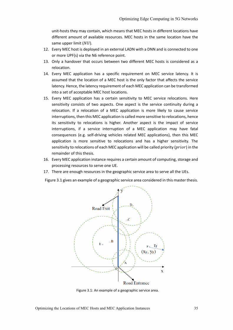
Optimizing Edge Computing in 5G Networks
Optimizing the Locations of MEC Hosts and MEC Application Instances 35
unit-hosts they may contain, which means that MEC hosts in different locations have
different amount of available resources. MEC hosts in the same location have the
same upper limit (𝑁𝑈).
12. Every MEC host is deployed in an external LADN with a DNN and is connected to one
or more UPF(s) via the N6 reference point.
13. Only a handover that occurs between two different MEC hosts is considered as a
relocation.
14. Every MEC application has a specific requirement on MEC service latency. It is
assumed that the location of a MEC host is the only factor that affects the service
latency. Hence, the latency requirement of each MEC application can be transformed
into a set of acceptable MEC host locations.
15. Every MEC application has a certain sensitivity to MEC service relocations. Here
sensitivity consists of two aspects. One aspect is the service continuity during a
relocation. If a relocation of a MEC application is more likely to cause service
interruptions, then this MEC application is called more sensitive to relocations, hence
its sensitivity to relocations is higher. Another aspect is the impact of service
interruptions, if a service interruption of a MEC application may have fatal
consequences (e.g. self-driving vehicles related MEC applications), then this MEC
application is more sensitive to relocations and has a higher sensitivity. The
sensitivity to relocations of each MEC application will be called priority (𝑝𝑟𝑖𝑜𝑟) in the
remainder of this thesis.
16. Every MEC application instance requires a certain amount of computing, storage and
processing resources to serve one UE.
17. There are enough resources in the geographic service area to serve all the UEs.
Figure 3.1 gives an example of a geographic service area considered in this master thesis.
Figure 3.1: An example of a geographic service area.
Optimizing Edge Computing in 5G Networks
Optimizing the Locations of MEC Hosts and MEC Application Instances 36
For each site (e.g. site 𝐹) in the geographic service area, its location information, which
is given as 𝑥, 𝑦 coordinates (e.g. (𝑥𝐹 , 𝑦𝐹)), as well as coverage radius 𝑟 (e.g. 𝑟𝐹) are known
in advance. A UE that enters the geographic service area will first be served by one of the
sites that cover the road entrance (e.g. site 𝐴, 𝐸). If a UE is served by one of the sites that
cover the road exit (e.g. site 𝐷), it will be served by this site until it leaves the geographic
serving area. Sites like site 𝐹 are unable to serve UEs on the road because its coverage circle
(the green circle with center point site 𝐹) does not intersect with the road (straight, blue
line).
The properties of MEC hosts introduced in assumption 8 lead to a dilemma regarding
the deployment of MEC hosts. If a MEC host is located far from the edge of the network and
close to the core network, the service latency between UEs and the MEC host will significantly
increase; if a MEC host is close to the edge of the network, the number of UEs it can serve
will significantly decrease, implying an increase in the number of relocations.
With the envisaged increase of MEC usage and the development of MEC applications,
there will be more MEC services required by users/applications/devices. In this situation, the
main driver of MEC is not latency but the availability of (enough) resources to serve the
increasing number of MEC users (see more in Appendix D). To make sure that the network
has enough resources in the worst situation in which the number of MEC users in the
geographic service area reaches the maximum number, enough resources and enough MEC
hosts should be provided. However, having a large number of MEC hosts can result in a large
number of relocations which may significantly degrade the user experience. Therefore, an
optimal deployment of MEC hosts and MEC applications needs to be determined in order to
minimize the number of relocations while still meeting the resource requirements.
3.2 Problem Formulation
A. Problem Description
Based on the assumptions above, research question 3 can be formulated as: given priority,
estimated UE flow, possible locations and required computing/storage/processing resources
of every MEC application, computing/storage/processing capacity of each unit-host as well
as the location and coverage of each site in the geographic service area, which unit-hosts
should be integrated as MEC hosts in each location and in which MEC hosts should the MEC
applications be installed, so as to minimize the total number of relocations and to provide
sufficient but not redundant resources?
In the above problem description, three key points can be extracted:
1. Optimization goal: Minimizing the total number of relocations
2. Guarantee continuous services for every UE
3. Reserve enough but not redundant resources for UEs of every MEC application. To
achieve this, an extreme situation is considered. The extreme situation is that UEs
are entering the geographic service area continuously, and at each time maximum
number of UEs enters together. This maximum number of UEs can be estimated based
on historical records (which types of UEs entered this area before and how many of
Optimizing Edge Computing in 5G Networks
Optimizing the Locations of MEC Hosts and MEC Application Instances 37
each type). Assume that all the UEs have the same, constant moving speed. Therefore,
in this extreme situation, the number of UEs at any location on the road at any time
is equal to the maximum number. The goal of the algorithm is to minimize the total
number of relocations in this extreme situation, while still meeting the requirements
on resources and service latency of each UE.
B. Problem Formulation
To minimize the total number of relocations, two steps need to be done:
Step 1: Find sites that can provide continuous MEC service for UEs. Set 𝐸1 records all the
unit-hosts that serve the sites that cover the entrance of the road, and set 𝐸2
records all the unit-hosts that serve the sites that cover the exit of the road.
Therefore, a UE will always get served by a unit-host which corresponds to one of
the sites in 𝐸1 as soon as it enters the geographic service area, and get served
by one of the sites in 𝐸2 when it leaves the area. To ensure service continuity,
shortest paths between one node in 𝐸1 and another node in 𝐸2 in graph 𝐺
need to be found. All the unit-hosts that belong to the same path are in the same
location, and this location is also the location of this path.
Step 2: After step 1 is done for every MEC application, find the approach to integrate unit-
hosts into MEC hosts and to minimize the number of relocations between these
MEC hosts.
All the paths in 𝐺 that are selected for MEC application 𝑘 can be denoted by the set
{𝑃𝑙𝑙𝑘(𝑛)}, ∀ 𝑙𝑙 ∈ 𝐿𝐿, ∀ 𝑛 ∈ {1, … , 𝑃𝑁𝑙𝑙(𝑘)} , while 𝑙𝑙 is the location of a path, 𝐿𝐿 is the set
that contains all possible locations of a unit-host and 𝑃𝑁𝑙𝑙(𝑘) is the total number of selected
paths in location 𝑙𝑙. The total path length selected for MEC application 𝑘 is
(4.1)
𝑃𝐿(𝑘) = ∑ ∑ 𝟏T ∙ 𝑃𝑙𝑙𝑘(𝑛) ∙ 𝟏
𝑃𝑁𝑙𝑙(𝑘)
𝑛=1𝑙𝑙∈𝐿𝐿
(3.1)
where 𝟏 represents an all-one vector, and here all-one vectors are used to calculate the
summation of all the elements in a matrix. Since the number of UEs of MEC application 𝑘
served by each path is different, then the total number of relocations of UEs of MEC
application 𝑘 experience is
(4.2) 𝑅𝐸(𝑘) = ∑ ∑ 𝑈𝐸𝑃𝑙𝑙𝑘(𝑛) ∙ [𝟏T ∙ 𝑃𝑙𝑙
𝑘(𝑛) ∙ 𝟏]
𝑃𝑁𝑙𝑙(𝑘)
𝑛=1𝑙𝑙∈𝐿𝐿
(3.2)
where 𝑈𝐸𝑃𝑙𝑙𝑘(𝑛) represents the number of UEs served by path 𝑛 in location 𝑙𝑙.
If a group of unit-hosts are integrated into one MEC host, then some relocations between
different unit-hosts will become relocations within one MEC host, which means that these
relocations are eliminated. Similarly, if several nodes in graph 𝐺 are merged as one node,
then some links will disappear. Consider the shortest paths {𝑃𝑙𝑙𝑘(𝑛)} mentioned above, the
number of disappeared links which belong to the paths selected for MEC application 𝑘 in
graph 𝐺 by merging nodes in the way that matrices {𝐻𝑙𝑙(𝑚)}(∀ 𝑙𝑙 ∈ 𝐿𝐿) imply is

Optimizing Edge Computing in 5G Networks
Optimizing the Locations of MEC Hosts and MEC Application Instances 38
(4.3)
𝐷𝐿(𝑘) = ∑ ∑ ∑ ∑ 𝑒𝑖T ∙ 𝑃𝑙𝑙
𝑘(𝑛) ∙ 𝐻𝑙𝑙(𝑚) ∙ 𝑒𝑖
𝑁
𝑖=1
𝐻𝑁𝑙𝑙
𝑚
𝑃𝑁𝑙𝑙(𝑘)
𝑛=1𝑙𝑙∈𝐿𝐿
(3.3)
where 𝐻𝑁𝑙𝑙 is the number of MEC hosts in location 𝑙𝑙 and matrix 𝐻𝑙𝑙(𝑚) indicates the
unit-hosts a MEC host contains and the links between these unit-hosts. Similarly, the total
number of eliminated relocations can be written as
(4.4)
𝐸𝑅(𝑘) = ∑ ∑ 𝑈𝐸𝑃𝑙𝑙𝑘(𝑛) ∙
𝑃𝑁𝑙𝑙(𝑘)
𝑛=1𝑙𝑙∈𝐿𝐿
∑ ∑ 𝑒𝑖T ∙ 𝑃𝑙𝑙
𝑘(𝑛) ∙ 𝐻𝑙𝑙(𝑚) ∙ 𝑒𝑖
𝑁
𝑖=1
𝐻𝑁𝑙𝑙
𝑚
(3.4)
Every MEC application has a priority which implies its importance. The MEC application
with a higher priority is more important. To distinguish different MEC applications, their
priorities also need to be considered. Therefore, the total weighted number of eliminated
relocations can be written as
(4.5) 𝐸𝑅𝑊(𝑘) = 𝑝𝑟𝑖𝑜𝑟𝑘 ∙ 𝐸𝑅(𝑘) (3.5)
where 𝑝𝑟𝑖𝑜𝑟𝑘 is the priority of MEC application 𝑘. Similarly, the total weighted number of
relocations before integrating unit-hosts into MEC hosts can be written as
(4.6) 𝑅𝐸𝑊(𝑘) = 𝑝𝑟𝑖𝑜𝑟𝑘 ∙ 𝑅𝐸(𝑘) (3.6)
The total weighted number of relocations of all MEC applications after integrating unit-
hosts into MEC hosts can be formulated as
(4.7)
𝑅𝑊 = ∑ 𝑅𝐸𝑊(𝑘) − 𝐸𝑅𝑊(𝑘)
𝑀
𝑘=1
(3.7)
where 𝑀 is the total number of MEC applications that need to be deployed. Therefore, the
optimization goal, minimizing the total number of relocations can be transformed into
minimizing 𝑅𝑊.
C. Constraints
To make sure that enough resources are allocated to UEs of every MEC application, Constraint
1 is defined as:
(3.8)
∑ ∑ 𝑈𝐸𝑃𝑙𝑙𝑘(𝑛)
𝑃𝑁𝑙𝑙(𝑘)
𝑛=1𝑙𝑙∈𝐿𝐿
≥ 𝑈𝐸𝑘 (∀ 𝑘 ∈ [1, … , 𝑀]) (3.8)
To make sure that every MEC host can meet the total resource requirements, the first
thing to do is to make sure that for each unit-host, its total amount of required resources
does not exceed its total amount of available resources. Sites in {𝑃𝑙𝑙𝑘(𝑛)} may have common
coverage area, where each of them may only need to serve some of the UEs. However, in the
context of this master thesis, each of these MEC hosts still needs to reserve enough resources
for all the UEs that are in its serving area for resiliency purpose. According to this, Constraint
2 is written as:
(3.9)
∑ ∑ 𝑈𝐸𝑃𝑙𝑙𝑘(𝑛) ∙ 𝑐𝑜𝑣𝑒𝑟𝑎𝑔𝑒𝑖
𝑃𝑁𝑙𝑙(𝑘)
𝑛=1
∙ 𝑐𝑟𝑘 ≤ 𝑐𝑟𝑢𝑛𝑖𝑡
𝑀
𝑘=1
(3.9)
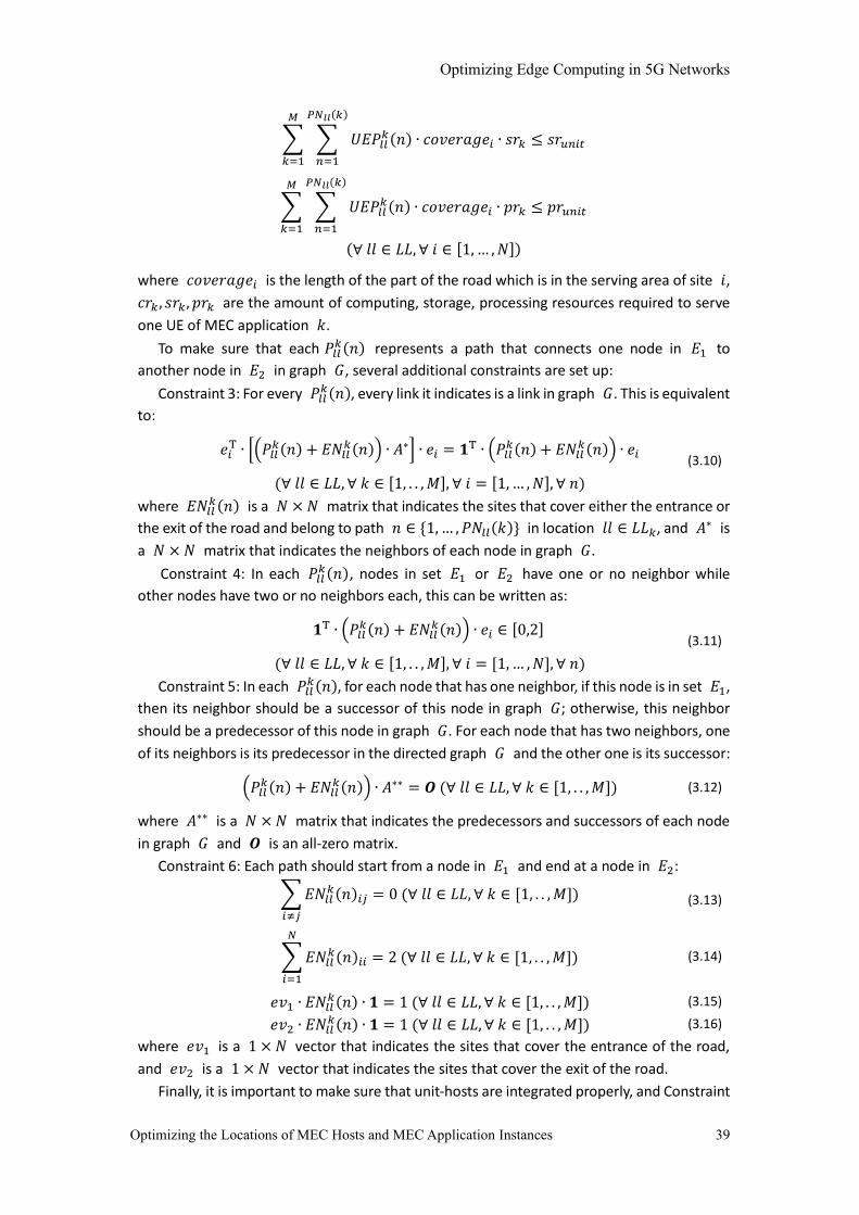
Optimizing Edge Computing in 5G Networks
Optimizing the Locations of MEC Hosts and MEC Application Instances 39
∑ ∑ 𝑈𝐸𝑃𝑙𝑙𝑘(𝑛) ∙ 𝑐𝑜𝑣𝑒𝑟𝑎𝑔𝑒𝑖
𝑃𝑁𝑙𝑙(𝑘)
𝑛=1
∙ 𝑠𝑟𝑘 ≤ 𝑠𝑟𝑢𝑛𝑖𝑡
𝑀
𝑘=1
∑ ∑ 𝑈𝐸𝑃𝑙𝑙𝑘(𝑛) ∙ 𝑐𝑜𝑣𝑒𝑟𝑎𝑔𝑒𝑖
𝑃𝑁𝑙𝑙(𝑘)
𝑛=1
∙ 𝑝𝑟𝑘 ≤ 𝑝𝑟𝑢𝑛𝑖𝑡
𝑀
𝑘=1
(∀ 𝑙𝑙 ∈ 𝐿𝐿, ∀ 𝑖 ∈ [1, … , 𝑁])
where 𝑐𝑜𝑣𝑒𝑟𝑎𝑔𝑒𝑖 is the length of the part of the road which is in the serving area of site 𝑖,
𝑐𝑟𝑘 , 𝑠𝑟𝑘, 𝑝𝑟𝑘 are the amount of computing, storage, processing resources required to serve
one UE of MEC application 𝑘.
To make sure that each 𝑃𝑙𝑙𝑘(𝑛) represents a path that connects one node in 𝐸1 to
another node in 𝐸2 in graph 𝐺, several additional constraints are set up:
Constraint 3: For every 𝑃𝑙𝑙𝑘(𝑛), every link it indicates is a link in graph 𝐺. This is equivalent
to:
(3.10) 𝑒𝑖
T ∙ [(𝑃𝑙𝑙𝑘(𝑛) + 𝐸𝑁𝑙𝑙
𝑘(𝑛)) ∙ 𝐴∗] ∙ 𝑒𝑖 = 𝟏T ∙ (𝑃𝑙𝑙𝑘(𝑛) + 𝐸𝑁𝑙𝑙
𝑘(𝑛)) ∙ 𝑒𝑖
(∀ 𝑙𝑙 ∈ 𝐿𝐿, ∀ 𝑘 ∈ [1, . . , 𝑀], ∀ 𝑖 = [1, … , 𝑁], ∀ 𝑛)
(3.10)
where 𝐸𝑁𝑙𝑙𝑘(𝑛) is a 𝑁 × 𝑁 matrix that indicates the sites that cover either the entrance or
the exit of the road and belong to path 𝑛 ∈ {1, … , 𝑃𝑁𝑙𝑙(𝑘)} in location 𝑙𝑙 ∈ 𝐿𝐿𝑘, and 𝐴∗ is
a 𝑁 × 𝑁 matrix that indicates the neighbors of each node in graph 𝐺.
Constraint 4: In each 𝑃𝑙𝑙𝑘(𝑛) , nodes in set 𝐸1 or 𝐸2 have one or no neighbor while
other nodes have two or no neighbors each, this can be written as:
(3.11) 𝟏T ∙ (𝑃𝑙𝑙
𝑘(𝑛) + 𝐸𝑁𝑙𝑙𝑘(𝑛)) ∙ 𝑒𝑖 ∈ [0,2]
(∀ 𝑙𝑙 ∈ 𝐿𝐿, ∀ 𝑘 ∈ [1, . . , 𝑀], ∀ 𝑖 = [1, … , 𝑁], ∀ 𝑛)
(3.11)
Constraint 5: In each 𝑃𝑙𝑙𝑘(𝑛), for each node that has one neighbor, if this node is in set 𝐸1,
then its neighbor should be a successor of this node in graph 𝐺; otherwise, this neighbor
should be a predecessor of this node in graph 𝐺. For each node that has two neighbors, one
of its neighbors is its predecessor in the directed graph 𝐺 and the other one is its successor:
(3.12) (𝑃𝑙𝑙
𝑘(𝑛) + 𝐸𝑁𝑙𝑙𝑘(𝑛)) ∙ 𝐴∗∗ = 𝑶 (∀ 𝑙𝑙 ∈ 𝐿𝐿, ∀ 𝑘 ∈ [1, . . , 𝑀]) (3.12)
where 𝐴∗∗ is a 𝑁 × 𝑁 matrix that indicates the predecessors and successors of each node
in graph 𝐺 and 𝑶 is an all-zero matrix.
Constraint 6: Each path should start from a node in 𝐸1 and end at a node in 𝐸2:
(3.13) ∑ 𝐸𝑁𝑙𝑙𝑘(𝑛)𝑖𝑗 = 0 (∀ 𝑙𝑙 ∈ 𝐿𝐿, ∀ 𝑘 ∈ [1, . . , 𝑀])
𝑖≠𝑗
(3.13)
∑ 𝐸𝑁𝑙𝑙𝑘(𝑛)𝑖𝑖 = 2 (∀ 𝑙𝑙 ∈ 𝐿𝐿, ∀ 𝑘 ∈ [1, . . , 𝑀])
𝑁
𝑖=1
(3.14)
𝑒𝑣1 ∙ 𝐸𝑁𝑙𝑙𝑘(𝑛) ∙ 𝟏 = 1 (∀ 𝑙𝑙 ∈ 𝐿𝐿, ∀ 𝑘 ∈ [1, . . , 𝑀]) (3.15)
𝑒𝑣2 ∙ 𝐸𝑁𝑙𝑙𝑘(𝑛) ∙ 𝟏 = 1 (∀ 𝑙𝑙 ∈ 𝐿𝐿, ∀ 𝑘 ∈ [1, . . , 𝑀]) (3.16)
where 𝑒𝑣1 is a 1 × 𝑁 vector that indicates the sites that cover the entrance of the road,
and 𝑒𝑣2 is a 1 × 𝑁 vector that indicates the sites that cover the exit of the road.
Finally, it is important to make sure that unit-hosts are integrated properly, and Constraint

Optimizing Edge Computing in 5G Networks
Optimizing the Locations of MEC Hosts and MEC Application Instances 40
7 is defined accordingly.
Constraint 7-1: There shall be no unit-host that is included in two MEC hosts:
(3.17)
∑ 𝑒𝑖T ∙ 𝐻𝑙𝑙(𝑚) ∙ 𝑒𝑖
𝐻𝑁𝑙
𝑚=1
≤ 1 (∀ 𝑙𝑙 ∈ 𝐿𝐿, ∀ 𝑖 ∈ [1, … , 𝑁]) (3.17)
Constraint 7-2: Every MEC host can meet the total resources requirements. It is
guaranteed by Equation 3.9 that the total amount of required resources of each unit-host
does not exceed its total amount of available resources. Therefore, in this step, it only needs
to be ensured that the number of unit-hosts that are integrated into one MEC host is smaller
than or equal to the upper limit 𝑁𝑈. This can be represented by inequation 3.18:
(3.18)
∑ 𝑒𝑖T ∙ 𝐻𝑙𝑙(𝑚) ∙ 𝑒𝑖 ≤ 𝑁𝑈𝑙𝑙 (∀ 𝑙𝑙 ∈ 𝐿𝐿, ∀ 𝑚 ∈ [1, … , 𝐻𝑁𝑙𝑙])
𝑁
𝑖= 1
(3.18)
D. Problem Decomposition
In the remainder of this chapter, approximation algorithms to minimize 𝑅𝑊 under the
seven constraints discussed in the previous section are designed, tested and compared. To
start with, the optimization problem needs to be decomposed.
In the original problem both MEC hosts and MEC applications need to be located.
Locations of MEC hosts need to be determined, and MEC applications need to be installed in
MEC hosts, which makes it impossible to determine the locations of MEC applications first
since they run on MEC hosts. However, information on MEC applications can help determine
the appropriate deployment of MEC hosts; without considering the MEC applications that
need to be deployed, it is difficult to determine how good a deployment of MEC hosts is. To
overcome this dilemma, the concept of “unit-host” has been brought up in this project. A
unit-host can be seen as a fraction of a MEC host with resources, MEC applications and MEC
application instances. These fractions can be combined into several complete MEC hosts. A
MEC host inherits all the resources, MEC applications and MEC application instances from
the unit-hosts it contains. Unit-hosts are not implemented and running in the telecom
network like MEC hosts, they are intermediate outcomes and will be eventually transformed
into MEC hosts.
Having defined the concept of “unit-host”, the original problem can be further
decomposed into two sub-problems, also called two phases in this thesis.
Phase 1: Locate enough but not redundant resources for each MEC application in unit-
hosts in its acceptable locations, in a way that the total number of relocations between unit-
hosts is minimized. Two algorithms - Greedy algorithm and Simulation based algorithm are
implemented and investigated in Phase 1.
Phase 2: Combine unit-hosts into MEC hosts properly. This sub-problem can be
transferred into a graph partitioning problem - minimum 𝑘-Cut problem, which can be either
NP-Hard or NP-Complete. If the number 𝑘 is not given, the problem is an NP-Hard problem.
The sub-problem to be solved in Phase 2 does not give the total number of MEC hosts in
advance, instead it is a factor that needs to be determined under certain constraints, hence,
this problem is NP-Hard. To solve such a problem, a purely greedy algorithm, two heuristic

Optimizing Edge Computing in 5G Networks
Optimizing the Locations of MEC Hosts and MEC Application Instances 41
algorithms (Variable Neighborhood Search and Multi-Kernighan Lin) have been implemented
and investigated in Phase 2.
3.3 Algorithms in Phase 1
In this section, two algorithms are proposed – greedy algorithm and simulation-based
algorithm. Both algorithms are used to solve the location problem of MEC applications in
Phase 1. The final goal of each algorithm is locating each MEC application in proper unit-hosts,
which can minimize the total number of relocations between unit-hosts in the geographic
service area under the extreme situation and guarantee enough resources as well as satisfied
service latency for each UE.
Based on the equations in section 3.2, four principles for deploying MEC applications in
unit-hosts are made:
1. Pick the shortest available path (with enough serving resources) between one node
in set 𝐸1 and one node in set 𝐸2 in graph 𝐺. In Equation 3.2, when there are fewer
1’s in matrix 𝑃𝑙𝑙𝑘(𝑛), which means that its corresponding path in graph 𝐺 is shorter,
𝑅𝐸(𝑘), ∃𝑘 ∈ {1,2, … , 𝑀} (the number of relocations between unit-hosts) tends to
be smaller. Therefore, MEC applications should be located in the unit-hosts which are
on the shortest available paths, which is also referred to as MEC applications should
be located in shortest paths in the remainder of the thesis.
2. Put more UEs on shorter paths. For each MEC application, enough resources should
be provided by the MEC hosts, which brings out Constraint 1 (defined by Equation
3.8). As discussed previously, a shortest available path, or an available path with
shortest length, means that a UE will experience the fewest relocations between
unit-hosts if it chooses this path. Therefore, to minimize 𝑅𝐸𝑊 , as many UEs as
possible should follow the shortest available path. Since the total number of
estimated UEs for each MEC application is fixed, if more UEs choose the shortest
available path, the total number of relocations will be reduced.
3. MEC applications with a higher priority should always be allocated resources to
earlier than the ones with a lower priority. MEC applications with a higher priority
are more sensitive to relocations. If a MEC application 1 is located in unit-hosts
before another MEC application 2 with a higher priority is located, MEC application
1 may fully occupy the resources in the unit-hosts that are on the shortest paths in
graph 𝐺 , as a consequence, MEC application 2 may be located in some other
longer paths. Since MEC application 2 is more sensitive to relocations, it does not
make sense to locate it in longer paths, therefore, allocating resources for MEC
applications with higher priority earlier than the ones with lower priority is the basic
rule in Phase 1.
4. Required service latency of each UE should be satisfied. The requirement on service
latency of each MEC application is transformed into a set of acceptable MEC
host/unit-host locations (assumption 14). To meet the required latency, each MEC
application is located only in the unit-hosts that are in its acceptable locations.
Considering the above four principles of MEC applications, greedy algorithm is a simple
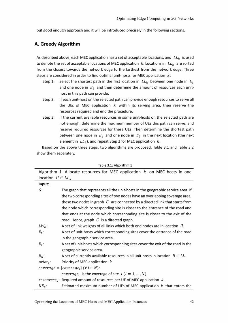
Optimizing Edge Computing in 5G Networks
Optimizing the Locations of MEC Hosts and MEC Application Instances 42
but good enough approach and it will be introduced precisely in the following sections.
A. Greedy Algorithm
As described above, each MEC application has a set of acceptable locations, and 𝐿𝐿𝑘 is used
to denote the set of acceptable locations of MEC application 𝑘. Locations in 𝐿𝐿𝑘 are sorted
from the closest towards the network edge to the farthest from the network edge. Three
steps are considered in order to find optimal unit-hosts for MEC application 𝑘:
Step 1: Select the shortest path in the first location in 𝐿𝐿𝑘 between one node in 𝐸1
and one node in 𝐸2 and then determine the amount of resources each unit-
host in this path can provide.
Step 2: If each unit-host on the selected path can provide enough resources to serve all
the UEs of MEC application 𝑘 within its serving area, then reserve the
resources required and end the procedure.
Step 3: If the current available resources in some unit-hosts on the selected path are
not enough, determine the maximum number of UEs this path can serve, and
reserve required resources for these UEs. Then determine the shortest path
between one node in 𝐸1 and one node in 𝐸2 in the next location (the next
element in 𝐿𝐿𝑘), and repeat Step 2 for MEC application 𝑘.
Based on the above three steps, two algorithms are proposed. Table 3.1 and Table 3.2
show them separately.
Table 3.1: Algorithm 1
Algorithm 1. Allocate resources for MEC application 𝑘 on MEC hosts in one
location 𝑙𝑙 ∈ 𝐿𝐿𝑘
Input:
𝐺: The graph that represents all the unit-hosts in the geographic service area. If
the two corresponding sites of two nodes have an overlapping coverage area,
these two nodes in graph 𝐺 are connected by a directed link that starts from
the node which corresponding site is closer to the entrance of the road and
that ends at the node which corresponding site is closer to the exit of the
road. Hence, graph 𝐺 is a directed graph.
𝐿𝑊𝑙𝑙: A set of link weights of all links which both end nodes are in location 𝑙𝑙.
𝐸1: A set of unit-hosts which corresponding sites cover the entrance of the road
in the geographic service area.
𝐸2: A set of unit-hosts which corresponding sites cover the exit of the road in the
geographic service area.
𝑅𝑙𝑙: A set of currently available resources in all unit-hosts in location 𝑙𝑙 ∈ 𝐿𝐿.
𝑝𝑟𝑖𝑜𝑟𝑘: Priority of MEC application 𝑘.
𝑐𝑜𝑣𝑒𝑟𝑎𝑔𝑒 = {𝑐𝑜𝑣𝑒𝑟𝑎𝑔𝑒𝑖} (∀ 𝑖 ∈ 𝑁):
𝑐𝑜𝑣𝑒𝑟𝑎𝑔𝑒𝑖 is the coverage of site 𝑖 (𝑖 = 1, … , 𝑁).
𝑟𝑒𝑠𝑜𝑢𝑟𝑐𝑒𝑠𝑘: Required amount of resources per UE of MEC application 𝑘.
𝑈𝐸𝑘: Estimated maximum number of UEs of MEC application 𝑘 that enters the
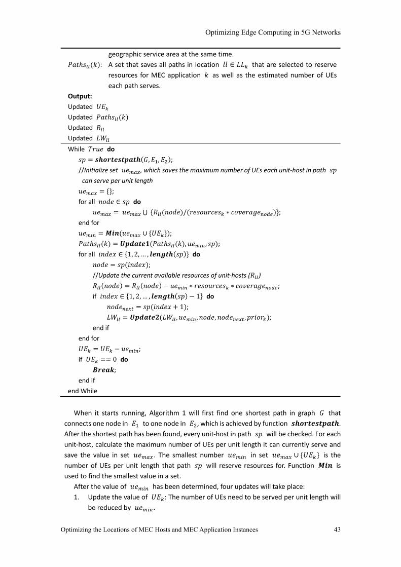
Optimizing Edge Computing in 5G Networks
Optimizing the Locations of MEC Hosts and MEC Application Instances 43
geographic service area at the same time.
𝑃𝑎𝑡ℎ𝑠𝑙𝑙(𝑘): A set that saves all paths in location 𝑙𝑙 ∈ 𝐿𝐿𝑘 that are selected to reserve
resources for MEC application 𝑘 as well as the estimated number of UEs
each path serves.
Output:
Updated 𝑈𝐸𝑘
Updated 𝑃𝑎𝑡ℎ𝑠𝑙𝑙(𝑘)
Updated 𝑅𝑙𝑙
Updated 𝐿𝑊𝑙𝑙
While 𝑇𝑟𝑢𝑒 do
𝑠𝑝 = 𝒔𝒉𝒐𝒓𝒕𝒆𝒔𝒕𝒑𝒂𝒕𝒉(𝐺, 𝐸1, 𝐸2);
//Initialize set 𝑢𝑒𝑚𝑎𝑥, which saves the maximum number of UEs each unit-host in path 𝑠𝑝
can serve per unit length
𝑢𝑒𝑚𝑎𝑥 = {};
for all 𝑛𝑜𝑑𝑒 ∈ 𝑠𝑝 do
𝑢𝑒𝑚𝑎𝑥 = 𝑢𝑒𝑚𝑎𝑥 ⋃ {𝑅𝑙𝑙(𝑛𝑜𝑑𝑒)/(𝑟𝑒𝑠𝑜𝑢𝑟𝑐𝑒𝑠𝑘 ∗ 𝑐𝑜𝑣𝑒𝑟𝑎𝑔𝑒𝑛𝑜𝑑𝑒)};
end for
𝑢𝑒𝑚𝑖𝑛 = 𝑴𝒊𝒏(𝑢𝑒𝑚𝑎𝑥 ∪ {𝑈𝐸𝑘});
𝑃𝑎𝑡ℎ𝑠𝑙𝑙(𝑘) = 𝑼𝒑𝒅𝒂𝒕𝒆𝟏(𝑃𝑎𝑡ℎ𝑠𝑙𝑙(𝑘), 𝑢𝑒𝑚𝑖𝑛, 𝑠𝑝);
for all 𝑖𝑛𝑑𝑒𝑥 ∈ {1, 2, … , 𝒍𝒆𝒏𝒈𝒕𝒉(𝑠𝑝)} do
𝑛𝑜𝑑𝑒 = 𝑠𝑝(𝑖𝑛𝑑𝑒𝑥);
//Update the current available resources of unit-hosts (𝑅𝑙𝑙)
𝑅𝑙𝑙(𝑛𝑜𝑑𝑒) = 𝑅𝑙𝑙(𝑛𝑜𝑑𝑒) − 𝑢𝑒𝑚𝑖𝑛 ∗ 𝑟𝑒𝑠𝑜𝑢𝑟𝑐𝑒𝑠𝑘 ∗ 𝑐𝑜𝑣𝑒𝑟𝑎𝑔𝑒𝑛𝑜𝑑𝑒;
if 𝑖𝑛𝑑𝑒𝑥 ∈ {1, 2, … , 𝒍𝒆𝒏𝒈𝒕𝒉(𝑠𝑝) − 1} do
𝑛𝑜𝑑𝑒𝑛𝑒𝑥𝑡 = 𝑠𝑝(𝑖𝑛𝑑𝑒𝑥 + 1);
𝐿𝑊𝑙𝑙 = 𝑼𝒑𝒅𝒂𝒕𝒆𝟐(𝐿𝑊𝑙𝑙 , 𝑢𝑒𝑚𝑖𝑛, 𝑛𝑜𝑑𝑒, 𝑛𝑜𝑑𝑒𝑛𝑒𝑥𝑡, 𝑝𝑟𝑖𝑜𝑟𝑘);
end if
end for
𝑈𝐸𝑘 = 𝑈𝐸𝑘 − 𝑢𝑒𝑚𝑖𝑛;
if 𝑈𝐸𝑘 == 0 do
𝑩𝒓𝒆𝒂𝒌;
end if
end While
When it starts running, Algorithm 1 will first find one shortest path in graph 𝐺 that
connects one node in 𝐸1 to one node in 𝐸2, which is achieved by function 𝒔𝒉𝒐𝒓𝒕𝒆𝒔𝒕𝒑𝒂𝒕𝒉.
After the shortest path has been found, every unit-host in path 𝑠𝑝 will be checked. For each
unit-host, calculate the maximum number of UEs per unit length it can currently serve and
save the value in set 𝑢𝑒𝑚𝑎𝑥 . The smallest number 𝑢𝑒𝑚𝑖𝑛 in set 𝑢𝑒𝑚𝑎𝑥 ∪ {𝑈𝐸𝑘} is the
number of UEs per unit length that path 𝑠𝑝 will reserve resources for. Function 𝑴𝒊𝒏 is
used to find the smallest value in a set.
After the value of 𝑢𝑒𝑚𝑖𝑛 has been determined, four updates will take place:
1. Update the value of 𝑈𝐸𝑘: The number of UEs need to be served per unit length will
be reduced by 𝑢𝑒𝑚𝑖𝑛.

Optimizing Edge Computing in 5G Networks
Optimizing the Locations of MEC Hosts and MEC Application Instances 44
2. Update 𝑃𝑎𝑡ℎ𝑠𝑙𝑙(𝑘): This is done by function 𝑼𝒑𝒅𝒂𝒕𝒆𝟏. To be more precise, if path
𝑠𝑝 has already been chosen by the same MEC application 𝑘, it should already exist
in 𝑃𝑎𝑡ℎ𝑠𝑙𝑙(𝑘), then 𝑼𝒑𝒅𝒂𝒕𝒆𝟏 will update its recorded number of serving UEs per
unit length by adding 𝑢𝑒𝑚𝑖𝑛 to the original value; if path 𝑠𝑝 does not exist in
𝑃𝑎𝑡ℎ𝑠𝑙𝑙(𝑘), then add a new record.
3. Update 𝑅𝑙𝑙 : Every unit-host on path 𝑠𝑝 will reserve new resources for MEC
application 𝑘, and their amount of available resources will decrease in the meantime.
For each unit-host, its corresponding record in 𝑅𝑙𝑙 needs to be updated. Function
𝒍𝒆𝒏𝒈𝒕𝒉 returns the number of elements in a set.
4. Update 𝐿𝑊𝑙𝑙 : This is done by function 𝑼𝒑𝒅𝒂𝒕𝒆𝟐 . Links in path 𝑠𝑝 represent
relocations. The link weight of a link is the weighted (by the priority of the MEC
application a UE uses) number of UEs per unit length on this link. Since new UEs are
added to each link, 𝐿𝑊𝑙𝑙 needs to be updated. For each link, update link weight by
adding 𝑝𝑟𝑖𝑜𝑟 ∗ 𝑢𝑒𝑚𝑖𝑛 to its current value.
Table 3.2: Algorithm 2
Algorithm 2: Allocate resources for MEC application 𝑘 in all its possible locations
Input:
𝐿𝐿𝑘: A set of possible locations for MEC application 𝑘.
𝑅 = {𝑅𝑙𝑙}, ∀ 𝑙𝑙 ∈ 𝐿𝐿:
𝑅𝑙𝑙 is the set of currently available resources in all unit-hosts in location 𝑙𝑙 ∈
𝐿𝐿.
𝐺: The directed graph that represents all the sites.
𝐸1: A set of unit-hosts which corresponding sites cover the entrance of the road
in the geographic service area.
𝐸2: A set of unit-hosts which corresponding sites cover the exit of the road in the
geographic service area.
𝐿𝑊 = {𝐿𝑊𝑙𝑙}, ∀ 𝑙𝑙 ∈ 𝐿𝐿:
𝐿𝑊𝑙𝑙 is the set of link weights of all links which both end nodes are in location
𝑙𝑙.
𝑃𝑎𝑡ℎ𝑠(𝑘) = {𝑃𝑎𝑡ℎ𝑠𝑙𝑙(𝑘)}, ∀ 𝑙𝑙 ∈ 𝐿𝐿𝑘:
𝑃𝑎𝑡ℎ𝑠𝑙𝑙(𝑘) is the set that saves all paths in location 𝑙𝑙 ∈ 𝐿𝐿𝑘 that are
selected to reserve resources for MEC application 𝑘 as well as the
estimated number of UEs each path serves.
𝑝𝑟𝑖𝑜𝑟𝑘: Priority of MEC application 𝑘.
𝑐𝑜𝑣𝑒𝑟𝑎𝑔𝑒 = {𝑐𝑜𝑣𝑒𝑟𝑎𝑔𝑒𝑖} (∀ 𝑖 ∈ 𝑁):
𝑐𝑜𝑣𝑒𝑟𝑎𝑔𝑒𝑖 is the coverage of site 𝑖 (𝑖 = 1, … , 𝑁).
𝑟𝑒𝑠𝑜𝑢𝑟𝑐𝑒𝑠𝑘: Required amount of resources per UE of MEC application 𝑘.𝑈𝐸𝑘: Estimated
number of UEs of MEC application 𝑘 that enters the geographic service area
at the same time.
Output:
Updated 𝑃𝑎𝑡ℎ𝑠(𝑘)
Updated 𝑅
Updated 𝐿𝑊

Optimizing Edge Computing in 5G Networks
Optimizing the Locations of MEC Hosts and MEC Application Instances 45
While True do
for all 𝑙𝑙 ∈ 𝐿𝐿𝑘 do
𝑈𝐸𝑘 , 𝐿𝑊𝑙𝑙 , 𝑃𝑎𝑡ℎ𝑠𝑙𝑙(𝑘), 𝑅𝑙𝑙 =
𝑨𝟏(𝑈𝐸𝑘 , 𝐺, 𝐿𝑊𝑙𝑙 , 𝐸1, 𝐸2, 𝑃𝑎𝑡ℎ𝑠𝑙𝑙(𝑘), 𝑅𝑙𝑙 , 𝑝𝑟𝑖𝑜𝑟𝑘 , 𝑐𝑜𝑣𝑒𝑟𝑎𝑔𝑒, 𝑟𝑒𝑠𝑜𝑢𝑟𝑐𝑒𝑠𝑘);
if 𝑈𝐸𝑘 == 0 do //Enough resources have been allocated
𝑩𝒓𝒆𝒂𝒌;
end if
end for
end While
Algorithm 2 is designed to allocate resources for MEC application 𝑘 in all its acceptable
locations if necessary. Function 𝑨𝟏 represents Algorithm 1 in Table 3.1.
B. Simulation-Based Algorithm
This algorithm is an improved greedy algorithm, and the improvement comes from the fact
that there are three different types of resources and the required amount of different types
of resources may be different. If well organized, one unit-host may be able to serve more UEs
without increasing the total amount of resources it holds. Figure 3.2 demonstrates the
difference between well-organized deployment and not well-organized deployment clearly.
Define ratio of a unit-host as the ratio of the available amount of three different types of
resources (computing, storage and processing) in the unit-host. The ratio before any
resources has been allocated/reserved is called the original ratio, and according to
assumption 6, original ratio = 1: 1: 1. For a group of MEC applications that have the same
priority 𝐴𝑃𝑃 = {𝑎𝑝𝑝1, 𝑎𝑝𝑝2, … , 𝑎𝑝𝑝𝑘}, and each with a required amount of resources which
is saved in vector 𝑅𝑅 = {𝑟11, 𝑟12, 𝑟13, … , 𝑟𝑘1, 𝑟𝑘2, 𝑟𝑘3} , where 𝑟𝑖1, 𝑟𝑖2, 𝑟𝑖3 represent the
required amount of computing, storage, processing resources of MEC application 𝑖
separately. If there exists a vector 𝑉 = {𝑣1, 𝑣2, … , 𝑣𝑘} , with 0 ≤ 𝑣𝑖 ≤ 𝑈𝐸𝑖 , 𝑣𝑖 ∈ 𝑁, ∀𝑖 ∈
{1,2, … , 𝑘} , and this vector 𝑉 has at least two non-zero elements, which satisfies the
following inequations:
(3.19) max
𝑗∈{1,2,3}
∑ 𝑟𝑖𝑗𝑣𝑖𝑘𝑖=𝑖
∑ 𝑣𝑖𝑘𝑖=1
≤ min𝑖∈{1,2,…,𝑘}
𝑣𝑖>0
max𝑗∈{1,2,3}
𝑟𝑖𝑗
𝑟11𝑣1 + 𝑟21𝑣2 + ⋯ + 𝑟𝑘1𝑣𝑘 < 𝑐𝑟𝑢𝑛𝑖𝑡
𝑟12𝑣1 + 𝑟22𝑣2 + ⋯ + 𝑟𝑘2𝑣𝑘 < 𝑠𝑟𝑢𝑛𝑖𝑡
𝑟13𝑣1 + 𝑟23𝑣2 + ⋯ + 𝑟𝑘3𝑣𝑘 < 𝑝𝑟𝑢𝑛𝑖𝑡
(3.19)
then MEC applications {𝑎𝑝𝑝𝑖|𝑖 ∈ {1,2, … , 𝑘}, 𝑣𝑖 > 0} are called a group of complementary
MEC applications.
Since it is assumed that the amount of computing, storage and processing resources in a
unit-host is equal (𝑐𝑟𝑢𝑛𝑖𝑡 = 𝑠𝑟𝑢𝑛𝑖𝑡 = 𝑝𝑟𝑢𝑛𝑖𝑡), then the type of resources which running a
MEC application instance to serve a UE needs the most determines the maximum number of
UEs one unit-host can serve. This type of resources is similar to the short slab of a bucket.
Complementary MEC applications have the same priority and can be deployed together to
even the usage of different types of resources and to make the short slab not short anymore.
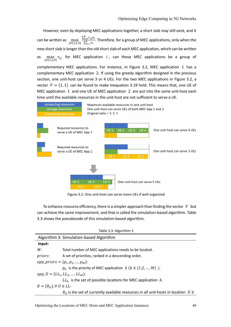
Optimizing Edge Computing in 5G Networks
Optimizing the Locations of MEC Hosts and MEC Application Instances 46
However, even by deploying MEC applications together, a short slab may still exist, and it
can be written as max𝑗∈{1,2,3}
∑ 𝑟𝑖𝑗𝑣𝑖𝑘𝑖=𝑖
∑ 𝑣𝑖𝑘𝑖=1
. Therefore, for a group of MEC applications, only when the
new short slab is longer than the old short slab of each MEC application, which can be written
as max𝑗∈{1,2,3}
𝑟𝑖𝑗 for MEC application 𝑖 , can these MEC applications be a group of
complementary MEC applications. For instance, in Figure 3.2, MEC application 1 has a
complementary MEC application 2. If using the greedy algorithm designed in the previous
section, one unit-host can serve 3 or 4 UEs. For the two MEC applications in Figure 3.2, a
vector 𝑉 = {1, 1} can be found to make Inequation 3.19 hold. This means that, one UE of
MEC application 1 and one UE of MEC application 2 are put into the same unit-host each
time until the available resources in the unit-host are not sufficient to serve a UE.
Figure 3.2: One unit-host can serve more UEs if well organized
To enhance resource efficiency, there is a simpler approach than finding the vector 𝑉 but
can achieve the same improvement, and that is called the simulation-based algorithm. Table
3.3 shows the pseudocode of this simulation-based algorithm.
Table 3.3: Algorithm 3
Algorithm 3. Simulation-based Algorithm
Input:
𝑀: Total number of MEC applications needs to be located.
𝑝𝑟𝑖𝑜𝑟𝑠: A set of priorities, ranked in a descending order.
𝑎𝑝𝑝_𝑝𝑟𝑖𝑜𝑟𝑠 = {𝑝1, 𝑝2, … , 𝑝𝑀}:
𝑝𝑘 is the priority of MEC application 𝑘 (𝑘 ∈ {1,2, … , 𝑀} ).
𝑎𝑝𝑝_𝑙𝑙 = {𝐿𝐿1, 𝐿𝐿2, … , 𝐿𝐿𝑀}:
𝐿𝐿𝑘 is the set of possible locations for MEC application 𝑘.
𝑅 = {𝑅𝑙𝑙}, ∀ 𝑙𝑙 ∈ 𝐿𝐿:
𝑅𝑙𝑙 is the set of currently available resources in all unit-hosts in location 𝑙𝑙 ∈

Optimizing Edge Computing in 5G Networks
Optimizing the Locations of MEC Hosts and MEC Application Instances 47
𝐿𝐿.
𝐺: The directed graph that represents all the sites.
𝐸1: A set of unit-hosts which corresponding sites cover the entrance of the road
in the geographic service area.
𝐸2: A set of unit-hosts which corresponding sites cover the exit of the road in the
geographic service area.
𝐿𝑊 = {𝐿𝑊𝑙𝑙}, ∀ 𝑙𝑙 ∈ 𝐿𝐿:
𝐿𝑊𝑙𝑙 is the set of link weights of all links which both end nodes are in location
𝑙𝑙.
𝑃𝑎𝑡ℎ𝑠 = {𝑃𝑎𝑡ℎ𝑠(𝑘)}, ∀ 𝑘 ∈ {1,2, … , 𝑀}:
𝑃𝑎𝑡ℎ𝑠(𝑘) records all the paths selected for MEC application 𝑘 and the number
of UEs each path serves.
𝑐𝑜𝑣𝑒𝑟𝑎𝑔𝑒: The set of coverage of all the site.
𝑟𝑒𝑠𝑜𝑢𝑟𝑐𝑒𝑠 = {𝑟𝑒𝑠𝑜𝑢𝑟𝑐𝑒𝑠1, 𝑟𝑒𝑠𝑜𝑢𝑟𝑐𝑒𝑠2, … , 𝑟𝑒𝑠𝑜𝑢𝑟𝑐𝑒𝑠𝑀}:
𝑟𝑒𝑠𝑜𝑢𝑟𝑐𝑒𝑠𝑘 is the required amount of resources per UE of MEC application
𝑘.
𝑈𝐸 = {𝑈𝐸1, 𝑈𝐸2, … , 𝑈𝐸𝑀}:
𝑈𝐸𝑘 is the estimated number of UEs of MEC application 𝑘 that enters the
geographic service area at the same time.
Output:
Updated 𝑃𝑎𝑡ℎ𝑠
Updated 𝑅
Updated 𝐿𝑊
for all 𝑝 ∈ 𝑝𝑟𝑖𝑜𝑟𝑠 do
𝑅𝑡𝑒𝑚𝑝 = {};
𝑃𝑎𝑡ℎ𝑠𝑡𝑒𝑚𝑝 = {};
𝐿𝑊𝑡𝑒𝑚𝑝 = {};
𝐷𝑖𝑓𝑓 = 𝑖𝑛𝑓;
𝑎𝑝𝑝𝑡𝑒𝑚𝑝 = 𝑁𝑜𝑛𝑒;
While ∃ 𝑎𝑝𝑝 ∈ 𝑀, 𝑎𝑝𝑝_𝑝𝑟𝑖𝑜𝑟𝑠(𝑎𝑝𝑝) == 𝑝 and 𝑈𝐸(𝑎𝑝𝑝) ≠ 0 do
for all 𝑎𝑝𝑝 ∈ 𝑀 do
if 𝑎𝑝𝑝_𝑝𝑟𝑖𝑜𝑟𝑠(𝑎𝑝𝑝) ! = 𝑝 or 𝑈𝐸(𝑎𝑝𝑝) == 0 do
𝑪𝒐𝒏𝒕𝒊𝒏𝒖𝒆;
end if
𝑃𝑎𝑡ℎ𝑠𝑡, 𝑅𝑡 , 𝐿𝑊𝑡 =
𝑨𝟐(𝑎𝑝𝑝_𝑙𝑙(𝑎𝑝𝑝), 𝑅, 𝐺, 𝐸1, 𝐸2, 𝐿𝑊, 𝑃𝑎𝑡ℎ𝑠(𝑎𝑝𝑝), 𝑝, 𝑐𝑜𝑣𝑒𝑟𝑎𝑔𝑒, 𝑟𝑒𝑠𝑜𝑢𝑟𝑐𝑒𝑠(𝑎𝑝𝑝),1);
𝑑𝑖𝑓𝑓 = 𝑫𝒊𝒇𝒇𝒆𝒓𝒆𝒏𝒄𝒆_𝒃𝒆𝒕𝒘𝒆𝒆𝒏_𝒓𝒂𝒕𝒊𝒐𝒔(𝑅𝑡);
if 𝑑𝑖𝑓𝑓 < 𝐷𝑖𝑓𝑓 do
𝑅𝑡𝑒𝑚𝑝 = 𝑅𝑡;
𝑃𝑎𝑡ℎ𝑠𝑡𝑒𝑚𝑝 = 𝑃𝑎𝑡ℎ𝑠𝑡;
𝐿𝑊𝑡𝑒𝑚𝑝 = 𝐿𝑊𝑡;
𝐷𝑖𝑓𝑓 = 𝑑𝑖𝑓𝑓;
𝑎𝑝𝑝𝑡𝑒𝑚𝑝 = 𝑎𝑝𝑝;
end if

Optimizing Edge Computing in 5G Networks
Optimizing the Locations of MEC Hosts and MEC Application Instances 48
end for
𝑃𝑎𝑡ℎ𝑠 = 𝑃𝑎𝑡ℎ𝑠𝑡𝑒𝑚𝑝;
𝑅 = 𝑅𝑡𝑒𝑚𝑝;
𝐿𝑊 = 𝐿𝑊𝑡𝑒𝑚𝑝;
𝑈𝐸(𝑎𝑝𝑝𝑡𝑒𝑚𝑝) = 𝑈𝐸(𝑎𝑝𝑝𝑡𝑒𝑚𝑝) − 1;
end While
end for
Define a simulation of MEC application 𝑎𝑝𝑝 as a process in which one UE using MEC
application 𝑎𝑝𝑝 is assumed to enter the geographic service area, a suitable path will be
selected for this UE, and resources will be reserved in the unit-hosts on the selected path.
Any operation in a simulation of MEC application 𝑎𝑝𝑝 will not affect the real network
conditions (e.g. the amount of available resources in a unit-host, the MEC applications
installed in a unit-host).
For every MEC application with the same priority, the algorithm will first do a simulation
of this MEC application, and calculate for each unit-host on the chosen path, if it reserves
resources for this UE, the difference between its ratio after resource reservation and the
original ratio, and then add these differences up. Function 𝑫𝒊𝒇𝒇𝒆𝒓𝒆𝒏𝒄𝒆_𝒃𝒆𝒕𝒘𝒆𝒆𝒏_𝒓𝒂𝒕𝒊𝒐𝒔
is responsible for the calculations, and the final result is saved in variable 𝑑𝑖𝑓𝑓. After every
MEC application has one simulation, pick the MEC application with the smallest 𝑑𝑖𝑓𝑓, and
then allocate resources for one UE of this MEC application in the unit-hosts on the path
selected in the simulation. This time the variables that reflect the actual network conditions
(e.g. 𝑅, 𝐿𝑊, 𝑃𝑎𝑡ℎ𝑠) need to be updated.
3.4 Algorithms in Phase 2
The goal of Phase 2 is to optimally integrate unit-hosts into MEC hosts in the three MEC host
locations mentioned in assumption 3. Consider the similarity of the three locations, once the
optimal locating mechanism of MEC hosts in one location is solved, then the integrations of
unit-hosts in the other two locations can use the same locating mechanism. Therefore, the
sub-problem needs to be solved in Phase 2 is to optimally location MEC hosts in one location,
and here locating a MEC host is to determine which unit-hosts it contains.
The above sub-problem can be transformed into a classical mathematical problem –
minimum 𝑘-cut problem: Given a graph 𝐺(𝑉, 𝐸), with node set 𝑉, link set 𝐸, and different
link weights on the links in link set 𝐸. The goal of the problem is to partition 𝑉 into several
disjoint subsets of limited sizes, in a way that minimizes the sum of the weights of the subset
of links that cross from one subset to another subset, which is denoted by 𝑇. In the context
of this specific sub-problem, graph 𝐺(𝑉, 𝐸) is the graph 𝐺 generated in Phase 1, node set
𝑉 is the collection of unit-hosts, a link weight is the weighted number of UEs per unit length
on the link. Each subset of nodes is a MEC host, which is considered as a collection of limited
number of unit-hosts. The limitation on number of unit-hosts 𝑁𝑈𝑙𝑙 depends on the location
𝑙𝑙 of one MEC host, and 𝑁𝑈𝑙𝑙 is larger if the location 𝑙𝑙 of the MEC host is closer to the
core network.
For minimum 𝑘 -cut problem, if the total number of subsets 𝑘 is given, then this
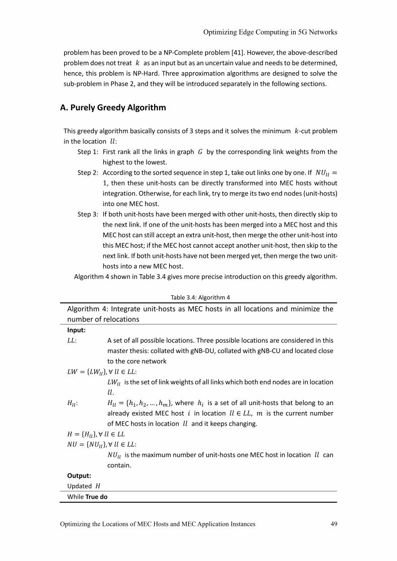
Optimizing Edge Computing in 5G Networks
Optimizing the Locations of MEC Hosts and MEC Application Instances 49
problem has been proved to be a NP-Complete problem [41]. However, the above-described
problem does not treat 𝑘 as an input but as an uncertain value and needs to be determined,
hence, this problem is NP-Hard. Three approximation algorithms are designed to solve the
sub-problem in Phase 2, and they will be introduced separately in the following sections.
A. Purely Greedy Algorithm
This greedy algorithm basically consists of 3 steps and it solves the minimum 𝑘-cut problem
in the location 𝑙𝑙:
Step 1: First rank all the links in graph 𝐺 by the corresponding link weights from the
highest to the lowest.
Step 2: According to the sorted sequence in step 1, take out links one by one. If 𝑁𝑈𝑙𝑙 =
1, then these unit-hosts can be directly transformed into MEC hosts without
integration. Otherwise, for each link, try to merge its two end nodes (unit-hosts)
into one MEC host.
Step 3: If both unit-hosts have been merged with other unit-hosts, then directly skip to
the next link. If one of the unit-hosts has been merged into a MEC host and this
MEC host can still accept an extra unit-host, then merge the other unit-host into
this MEC host; if the MEC host cannot accept another unit-host, then skip to the
next link. If both unit-hosts have not been merged yet, then merge the two unit-
hosts into a new MEC host.
Algorithm 4 shown in Table 3.4 gives more precise introduction on this greedy algorithm.
Table 3.4: Algorithm 4
Algorithm 4: Integrate unit-hosts as MEC hosts in all locations and minimize the
number of relocations
Input:
𝐿𝐿: A set of all possible locations. Three possible locations are considered in this
master thesis: collated with gNB-DU, collated with gNB-CU and located close
to the core network
𝐿𝑊 = {𝐿𝑊𝑙𝑙}, ∀ 𝑙𝑙 ∈ 𝐿𝐿:
𝐿𝑊𝑙𝑙 is the set of link weights of all links which both end nodes are in location
𝑙𝑙.
𝐻𝑙𝑙: 𝐻𝑙𝑙 = {ℎ1, ℎ2, … , ℎ𝑚}, where ℎ𝑖 is a set of all unit-hosts that belong to an
already existed MEC host 𝑖 in location 𝑙𝑙 ∈ 𝐿𝐿, 𝑚 is the current number
of MEC hosts in location 𝑙𝑙 and it keeps changing.
𝐻 = {𝐻𝑙𝑙}, ∀ 𝑙𝑙 ∈ 𝐿𝐿
𝑁𝑈 = {𝑁𝑈𝑙𝑙}, ∀ 𝑙𝑙 ∈ 𝐿𝐿:
𝑁𝑈𝑙𝑙 is the maximum number of unit-hosts one MEC host in location 𝑙𝑙 can
contain.
Output:
Updated 𝐻
While True do

Optimizing Edge Computing in 5G Networks
Optimizing the Locations of MEC Hosts and MEC Application Instances 50
for all 𝑙𝑙 ∈ 𝐿𝐿 do
for 𝑒 ∈ 𝒔𝒐𝒓𝒕(𝐿𝑊𝑙𝑙) do
𝑛𝑜𝑑𝑒𝑖𝑛 = 𝑒(1);
𝑛𝑜𝑑𝑒𝑜𝑢𝑡 = 𝑒(2);
if 𝑛𝑜𝑑𝑒𝑖𝑛 ∉ 𝐻𝑙𝑙 and 𝑛𝑜𝑑𝑒𝑜𝑢𝑡 ∉ 𝐻𝑙𝑙 do
if 𝑁𝑈𝑙𝑙 ≥ 2 do
𝐻𝑙𝑙 = 𝐻𝑙𝑙 ∪ {{𝑛𝑜𝑑𝑒𝑖𝑛, 𝑛𝑜𝑑𝑒𝑜𝑢𝑡}};
else do
𝐻𝑙𝑙 = 𝐻𝑙𝑙 ∪ {{𝑛𝑜𝑑𝑒𝑖𝑛}};
𝐻𝑙𝑙 = 𝐻𝑙𝑙 ∪ {{𝑛𝑜𝑑𝑒𝑜𝑢𝑡}};
end if
end if
if 𝑛𝑜𝑑𝑒𝑖𝑛 ∉ 𝐻𝑙𝑙 and 𝑛𝑜𝑑𝑒𝑜𝑢𝑡 ∈ 𝐻𝑙𝑙 do
ℎ𝑜𝑠𝑡 = 𝒇𝒊𝒏𝒅_𝒉𝒐𝒔𝒕(𝐻𝑙𝑙, 𝑛𝑜𝑑𝑒𝑜𝑢𝑡);
if 𝒍𝒆𝒏𝒈𝒕𝒉(ℎ𝑜𝑠𝑡) ≤ 𝑁𝑈𝑙𝑙 do
ℎ𝑜𝑠𝑡 = ℎ𝑜𝑠𝑡 ∪ {𝑛𝑜𝑑𝑒𝑖𝑛};
else do
𝐻𝑙𝑙 = 𝐻𝑙𝑙 ∪ {{𝑛𝑜𝑑𝑒𝑖𝑛}};
end if
end if
if 𝑛𝑜𝑑𝑒𝑜𝑢𝑡 ∉ 𝐻𝑙𝑙 and 𝑛𝑜𝑑𝑒𝑖𝑛 ∈ 𝐻𝑙𝑙 do
ℎ𝑜𝑠𝑡 = 𝒇𝒊𝒏𝒅_𝒉𝒐𝒔𝒕(𝐻𝑙𝑙, 𝑛𝑜𝑑𝑒𝑖𝑛);
if 𝒍𝒆𝒏𝒈𝒕𝒉(ℎ𝑜𝑠𝑡) ≤ 𝑁𝑈𝑙𝑙 do
ℎ𝑜𝑠𝑡 = ℎ𝑜𝑠𝑡 ∪ {𝑛𝑜𝑑𝑒𝑜𝑢𝑡};
else do
𝐻𝑙𝑙 = 𝐻𝑙𝑙 ∪ {{𝑛𝑜𝑑𝑒𝑜𝑢𝑡}};
end if
end if
end for
end for
𝑩𝒓𝒆𝒂𝒌;
end While
In Table 3.4, function 𝒔𝒐𝒓𝒕 is responsible for sorting all links in graph 𝐺 by their link
weights in descending order. If a unit-host has already been merged into a MEC host, function
𝒇𝒊𝒏𝒅_𝒉𝒐𝒔𝒕 is used to find which MEC host it belong to and the other unit-hosts this MEC
host contains.
B. Heuristic Algorithm – Variable Neighbor Search (VNS)
Since a greedy algorithm may not be able to give satisfactory results, to find better solutions,
a heuristic algorithm called Variable Neighbor Search (VNS) is used in Phase 2.
The concept of a neighborhood of a point represents a set of points containing the original
point where one can move some amount in any direction away from that point without

Optimizing Edge Computing in 5G Networks
Optimizing the Locations of MEC Hosts and MEC Application Instances 51
leaving the set. In neighbor search algorithms, an operation can be taken to transfer a point
into one of its neighbors, and by repeatedly doing so, one neighborhood of this point can be
generated. Obviously, there are usually multiple choices of possible operations, which results
in multiple neighborhoods for one point.
In Phase 2, a point is a solution, or a possible combination of unit-hosts, whose neighbor
is another similar solution derived from itself by taking an operation. Neighbors generated
by the same operation make a neighborhood.
Variable Neighbor Search (VNS) is a heuristic algorithm which is used to approximate a
solution for NP-Hard optimization problems. VNS algorithm is based on the local search
algorithm, which outcome tends to fall into a local optimum and never gets out. VNS is an
improved local search algorithm because it has mechanism that can force it to step out of the
local optimum.
VNS consists of two main steps: Variable Neighborhood Descent and Shaking Procedure.
Variable Neighborhood Descent (VND)
The pseudocode of VND is shown in Table 3.5.
Table 3.5: Variable Neighbor Descent
Procedure VND
Input:
𝑥: The original solution.
𝑛𝑒: The number of neighborhoods provided.
𝑁𝐸 = {𝑁𝐸𝑖}, 𝑖 = {1,2, … , 𝑛𝑒}:
𝑁𝐸𝑖 is the 𝑖-th neighborhood.
Output:
Updated 𝑥
𝑖 = 1;
While 𝑇𝑟𝑢𝑒 do
𝑥′ = 𝒍𝒐𝒄𝒂𝒍_𝒔𝒆𝒂𝒓𝒄𝒉(𝑁𝐸(𝑖), 𝑥);
if 𝑥′ ≠ 𝑥 do
𝑖 = 1;
𝑥 = 𝑥′;
else
𝑖 = 𝑖 + 1;
end if
if 𝑖 > 𝑛𝑒 do
𝑩𝒓𝒆𝒂𝒌;
end if
end While
First of all, there should be an original solution 𝑥 as an input to VND. This solution can
be a random solution, or a sub-optimal solution derived from simpler algorithms, for example,
greedy algorithm. Besides, 𝑛𝑒 neighborhoods should be pre-determined. The algorithm has
four steps listed below:
1. Select the first neighborhood 𝑁1 and continue with step 2.
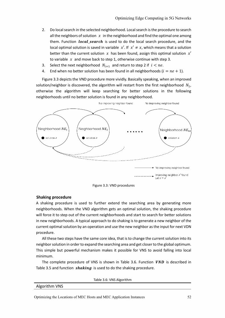
Optimizing Edge Computing in 5G Networks
Optimizing the Locations of MEC Hosts and MEC Application Instances 52
2. Do local search in the selected neighborhood. Local search is the procedure to search
all the neighbors of solution 𝑥 in the neighborhood and find the optimal one among
them. Function 𝒍𝒐𝒄𝒂𝒍_𝒔𝒆𝒂𝒓𝒄𝒉 is used to do the local search procedure, and the
local optimal solution is saved in variable 𝑥′. If 𝑥′ ≠ 𝑥, which means that a solution
better than the current solution 𝑥 has been found, assign this optimal solution 𝑥′
to variable 𝑥 and move back to step 1, otherwise continue with step 3.
3. Select the next neighborhood 𝑁𝑖+1 and return to step 2 if 𝑖 < 𝑛𝑒.
4. End when no better solution has been found in all neighborhoods (𝑖 = 𝑛𝑒 + 1).
Figure 3.3 depicts the VND procedure more vividly. Basically speaking, when an improved
solution/neighbor is discovered, the algorithm will restart from the first neighborhood 𝑁1,
otherwise the algorithm will keep searching for better solutions in the following
neighborhoods until no better solution is found in any neighborhood.
Figure 3.3: VND procedures
Shaking procedure
A shaking procedure is used to further extend the searching area by generating more
neighborhoods. When the VND algorithm gets an optimal solution, the shaking procedure
will force it to step out of the current neighborhoods and start to search for better solutions
in new neighborhoods. A typical approach to do shaking is to generate a new neighbor of the
current optimal solution by an operation and use the new neighbor as the input for next VDN
procedure.
All these two steps have the same core idea, that is to change the current solution into its
neighbor solution in order to expand the searching area and get closer to the global optimum.
This simple but powerful mechanism makes it possible for VNS to avoid falling into local
minimum.
The complete procedure of VNS is shown in Table 3.6. Function 𝑽𝑵𝑫 is described in
Table 3.5 and function 𝒔𝒉𝒂𝒌𝒊𝒏𝒈 is used to do the shaking procedure.
Table 3.6: VNS Algorithm
Algorithm VNS
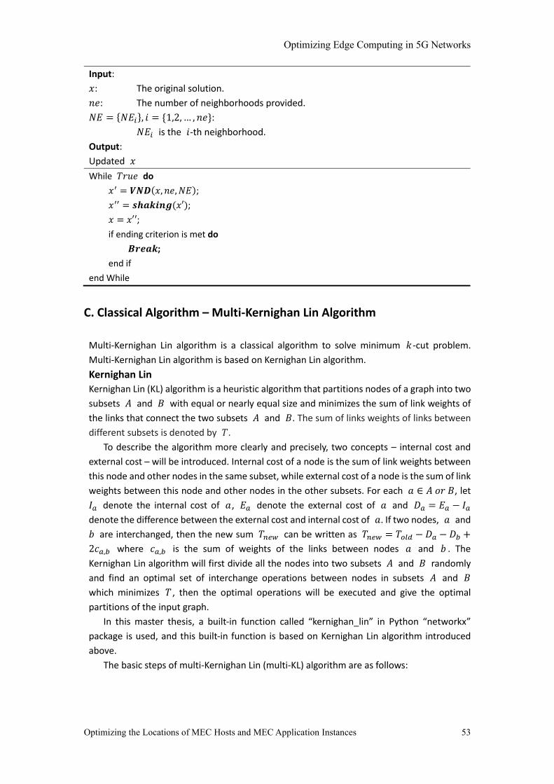
Optimizing Edge Computing in 5G Networks
Optimizing the Locations of MEC Hosts and MEC Application Instances 53
Input:
𝑥: The original solution.
𝑛𝑒: The number of neighborhoods provided.
𝑁𝐸 = {𝑁𝐸𝑖}, 𝑖 = {1,2, … , 𝑛𝑒}:
𝑁𝐸𝑖 is the 𝑖-th neighborhood.
Output:
Updated 𝑥
While 𝑇𝑟𝑢𝑒 do
𝑥′ = 𝑽𝑵𝑫(𝑥, 𝑛𝑒, 𝑁𝐸);
𝑥′′ = 𝒔𝒉𝒂𝒌𝒊𝒏𝒈(𝑥′);
𝑥 = 𝑥′′;
if ending criterion is met do
𝑩𝒓𝒆𝒂𝒌;
end if
end While
C. Classical Algorithm – Multi-Kernighan Lin Algorithm
Multi-Kernighan Lin algorithm is a classical algorithm to solve minimum 𝑘 -cut problem.
Multi-Kernighan Lin algorithm is based on Kernighan Lin algorithm.
Kernighan Lin
Kernighan Lin (KL) algorithm is a heuristic algorithm that partitions nodes of a graph into two
subsets 𝐴 and 𝐵 with equal or nearly equal size and minimizes the sum of link weights of
the links that connect the two subsets 𝐴 and 𝐵. The sum of links weights of links between
different subsets is denoted by 𝑇.
To describe the algorithm more clearly and precisely, two concepts – internal cost and
external cost – will be introduced. Internal cost of a node is the sum of link weights between
this node and other nodes in the same subset, while external cost of a node is the sum of link
weights between this node and other nodes in the other subsets. For each 𝑎 ∈ 𝐴 𝑜𝑟 𝐵, let
𝐼𝑎 denote the internal cost of 𝑎 , 𝐸𝑎 denote the external cost of 𝑎 and 𝐷𝑎 = 𝐸𝑎 − 𝐼𝑎
denote the difference between the external cost and internal cost of 𝑎. If two nodes, 𝑎 and
𝑏 are interchanged, then the new sum 𝑇𝑛𝑒𝑤 can be written as 𝑇𝑛𝑒𝑤 = 𝑇𝑜𝑙𝑑 − 𝐷𝑎 − 𝐷𝑏 +
2𝑐𝑎,𝑏 where 𝑐𝑎,𝑏 is the sum of weights of the links between nodes 𝑎 and 𝑏 . The
Kernighan Lin algorithm will first divide all the nodes into two subsets 𝐴 and 𝐵 randomly
and find an optimal set of interchange operations between nodes in subsets 𝐴 and 𝐵
which minimizes 𝑇 , then the optimal operations will be executed and give the optimal
partitions of the input graph.
In this master thesis, a built-in function called “kernighan_lin” in Python “networkx”
package is used, and this built-in function is based on Kernighan Lin algorithm introduced
above.
The basic steps of multi-Kernighan Lin (multi-KL) algorithm are as follows:
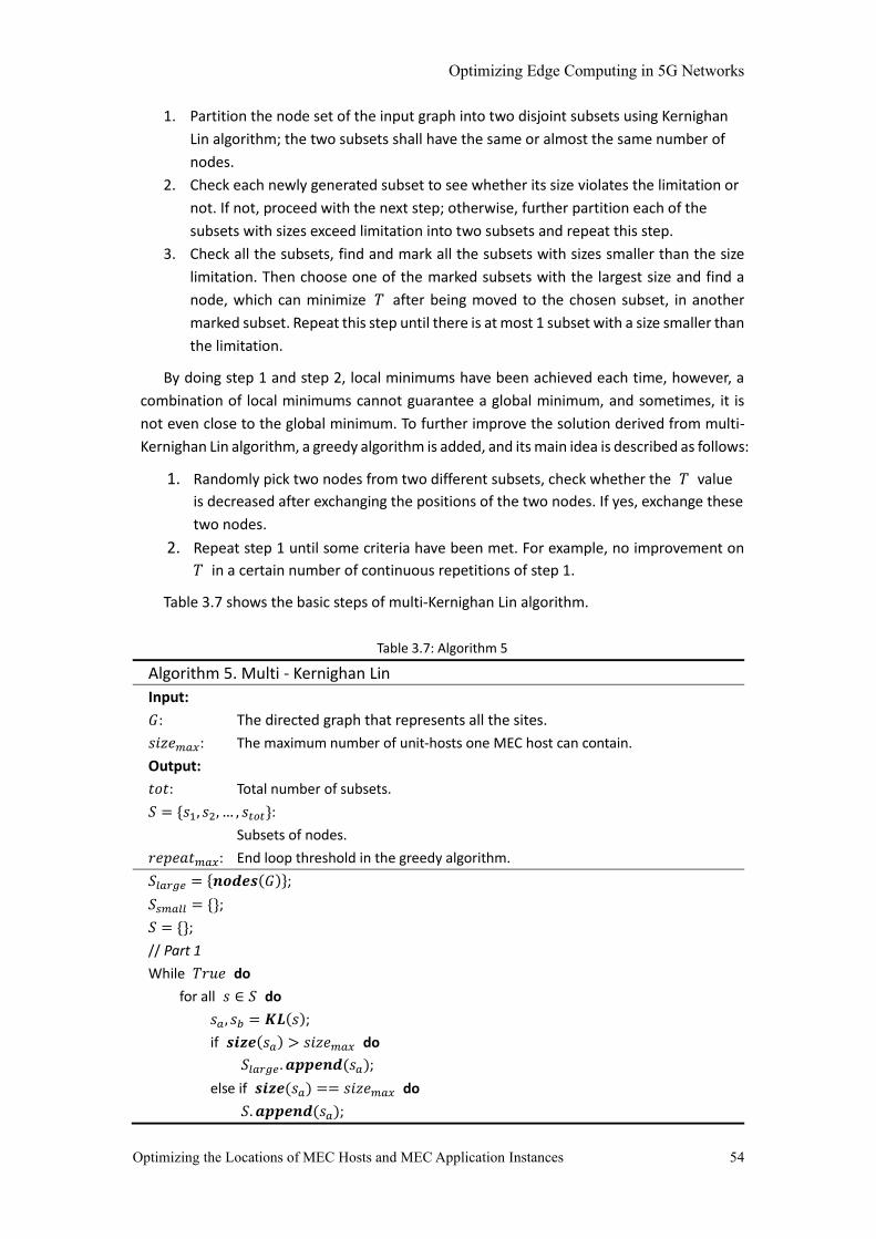
Optimizing Edge Computing in 5G Networks
Optimizing the Locations of MEC Hosts and MEC Application Instances 54
1. Partition the node set of the input graph into two disjoint subsets using Kernighan
Lin algorithm; the two subsets shall have the same or almost the same number of
nodes.
2. Check each newly generated subset to see whether its size violates the limitation or
not. If not, proceed with the next step; otherwise, further partition each of the
subsets with sizes exceed limitation into two subsets and repeat this step.
3. Check all the subsets, find and mark all the subsets with sizes smaller than the size
limitation. Then choose one of the marked subsets with the largest size and find a
node, which can minimize 𝑇 after being moved to the chosen subset, in another
marked subset. Repeat this step until there is at most 1 subset with a size smaller than
the limitation.
By doing step 1 and step 2, local minimums have been achieved each time, however, a
combination of local minimums cannot guarantee a global minimum, and sometimes, it is
not even close to the global minimum. To further improve the solution derived from multi-
Kernighan Lin algorithm, a greedy algorithm is added, and its main idea is described as follows:
1. Randomly pick two nodes from two different subsets, check whether the 𝑇 value
is decreased after exchanging the positions of the two nodes. If yes, exchange these
two nodes.
2. Repeat step 1 until some criteria have been met. For example, no improvement on
𝑇 in a certain number of continuous repetitions of step 1.
Table 3.7 shows the basic steps of multi-Kernighan Lin algorithm.
Table 3.7: Algorithm 5
Algorithm 5. Multi - Kernighan Lin
Input:
𝐺: The directed graph that represents all the sites.
𝑠𝑖𝑧𝑒𝑚𝑎𝑥: The maximum number of unit-hosts one MEC host can contain.
Output:
𝑡𝑜𝑡: Total number of subsets.
𝑆 = {𝑠1, 𝑠2, … , 𝑠𝑡𝑜𝑡}:
Subsets of nodes.
𝑟𝑒𝑝𝑒𝑎𝑡𝑚𝑎𝑥: End loop threshold in the greedy algorithm.
𝑆𝑙𝑎𝑟𝑔𝑒 = {𝒏𝒐𝒅𝒆𝒔(𝐺)};
𝑆𝑠𝑚𝑎𝑙𝑙 = {};
𝑆 = {};
// Part 1
While 𝑇𝑟𝑢𝑒 do
for all 𝑠 ∈ 𝑆 do
𝑠𝑎 , 𝑠𝑏 = 𝑲𝑳(𝑠);
if 𝒔𝒊𝒛𝒆(𝑠𝑎) > 𝑠𝑖𝑧𝑒𝑚𝑎𝑥 do
𝑆𝑙𝑎𝑟𝑔𝑒. 𝒂𝒑𝒑𝒆𝒏𝒅(𝑠𝑎);
else if 𝒔𝒊𝒛𝒆(𝑠𝑎) == 𝑠𝑖𝑧𝑒𝑚𝑎𝑥 do
𝑆. 𝒂𝒑𝒑𝒆𝒏𝒅(𝑠𝑎);
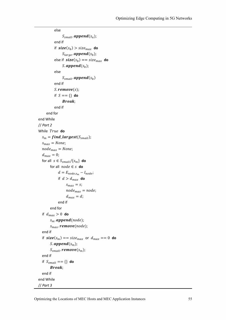
Optimizing Edge Computing in 5G Networks
Optimizing the Locations of MEC Hosts and MEC Application Instances 55
else
𝑆𝑠𝑚𝑎𝑙𝑙 . 𝒂𝒑𝒑𝒆𝒏𝒅(𝑠𝑎);
end if
if 𝒔𝒊𝒛𝒆(𝑠𝑏) > 𝑠𝑖𝑧𝑒𝑚𝑎𝑥 do
𝑆𝑙𝑎𝑟𝑔𝑒. 𝒂𝒑𝒑𝒆𝒏𝒅(𝑠𝑏);
else if 𝒔𝒊𝒛𝒆(𝑠𝑏) == 𝑠𝑖𝑧𝑒𝑚𝑎𝑥 do
𝑆. 𝒂𝒑𝒑𝒆𝒏𝒅(𝑠𝑏);
else
𝑆𝑠𝑚𝑎𝑙𝑙 . 𝒂𝒑𝒑𝒆𝒏𝒅(𝑠𝑏)
end if
𝑆. 𝒓𝒆𝒎𝒐𝒗𝒆(𝑠);
if 𝑆 == {} do
𝑩𝒓𝒆𝒂𝒌;
end if
end for
end While
// Part 2
While 𝑇𝑟𝑢𝑒 do
𝑠𝑚 = 𝒇𝒊𝒏𝒅_𝒍𝒂𝒓𝒈𝒆𝒔𝒕(𝑆𝑠𝑚𝑎𝑙𝑙);
𝑠𝑚𝑎𝑥 = 𝑁𝑜𝑛𝑒;
𝑛𝑜𝑑𝑒𝑚𝑎𝑥 = 𝑁𝑜𝑛𝑒;
𝑑𝑚𝑎𝑥 = 0;
for all 𝑠 ∈ 𝑆𝑠𝑚𝑎𝑙𝑙/{𝑠𝑚} do
for all 𝑛𝑜𝑑𝑒 ∈ 𝑠 do
𝑑 = 𝐸𝑛𝑜𝑑𝑒,𝑠𝑚− 𝐼𝑛𝑜𝑑𝑒;
if 𝑑 > 𝑑𝑚𝑎𝑥 do
𝑠𝑚𝑎𝑥 = 𝑠;
𝑛𝑜𝑑𝑒𝑚𝑎𝑥 = 𝑛𝑜𝑑𝑒;
𝑑𝑚𝑎𝑥 = 𝑑;
end if
end for
if 𝑑𝑚𝑎𝑥 > 0 do
𝑠𝑚. 𝒂𝒑𝒑𝒆𝒏𝒅(𝑛𝑜𝑑𝑒);
𝑠𝑚𝑎𝑥. 𝒓𝒆𝒎𝒐𝒗𝒆(𝑛𝑜𝑑𝑒);
end if
if 𝒔𝒊𝒛𝒆(𝑠𝑚) == 𝑠𝑖𝑧𝑒𝑚𝑎𝑥 or 𝑑𝑚𝑎𝑥 == 0 do
𝑆. 𝒂𝒑𝒑𝒆𝒏𝒅(𝑠𝑚);
𝑆𝑠𝑚𝑎𝑙𝑙 . 𝒓𝒆𝒎𝒐𝒗𝒆(𝑠𝑚);
end if
if 𝑆𝑠𝑚𝑎𝑙𝑙 == {} do
𝑩𝒓𝒆𝒂𝒌;
end if
end While
// Part 3
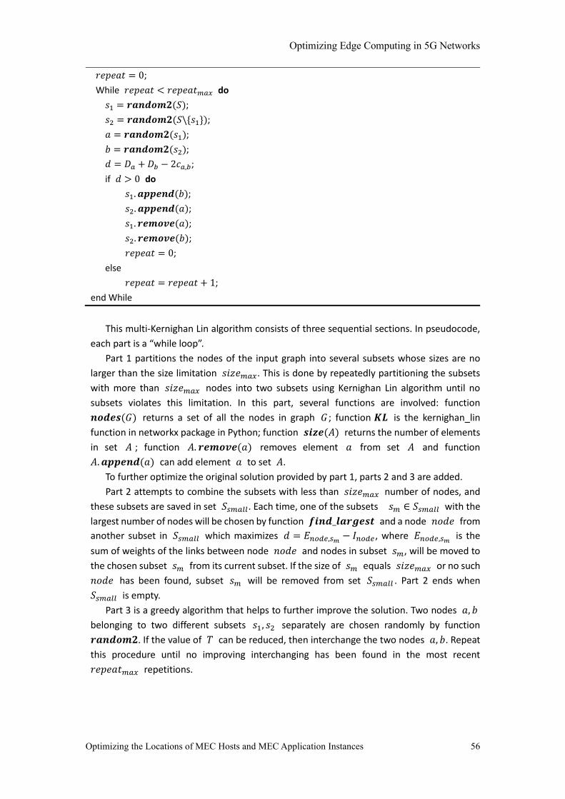
Optimizing Edge Computing in 5G Networks
Optimizing the Locations of MEC Hosts and MEC Application Instances 56
𝑟𝑒𝑝𝑒𝑎𝑡 = 0;
While 𝑟𝑒𝑝𝑒𝑎𝑡 < 𝑟𝑒𝑝𝑒𝑎𝑡𝑚𝑎𝑥 do
𝑠1 = 𝒓𝒂𝒏𝒅𝒐𝒎𝟐(𝑆);
𝑠2 = 𝒓𝒂𝒏𝒅𝒐𝒎𝟐(𝑆\{𝑠1});
𝑎 = 𝒓𝒂𝒏𝒅𝒐𝒎𝟐(𝑠1);
𝑏 = 𝒓𝒂𝒏𝒅𝒐𝒎𝟐(𝑠2);
𝑑 = 𝐷𝑎 + 𝐷𝑏 − 2𝑐𝑎,𝑏;
if 𝑑 > 0 do
𝑠1. 𝒂𝒑𝒑𝒆𝒏𝒅(𝑏);
𝑠2. 𝒂𝒑𝒑𝒆𝒏𝒅(𝑎);
𝑠1. 𝒓𝒆𝒎𝒐𝒗𝒆(𝑎);
𝑠2. 𝒓𝒆𝒎𝒐𝒗𝒆(𝑏);
𝑟𝑒𝑝𝑒𝑎𝑡 = 0;
else
𝑟𝑒𝑝𝑒𝑎𝑡 = 𝑟𝑒𝑝𝑒𝑎𝑡 + 1;
end While
This multi-Kernighan Lin algorithm consists of three sequential sections. In pseudocode,
each part is a “while loop”.
Part 1 partitions the nodes of the input graph into several subsets whose sizes are no
larger than the size limitation 𝑠𝑖𝑧𝑒𝑚𝑎𝑥. This is done by repeatedly partitioning the subsets
with more than 𝑠𝑖𝑧𝑒𝑚𝑎𝑥 nodes into two subsets using Kernighan Lin algorithm until no
subsets violates this limitation. In this part, several functions are involved: function
𝒏𝒐𝒅𝒆𝒔(𝐺) returns a set of all the nodes in graph 𝐺 ; function 𝑲𝑳 is the kernighan_lin
function in networkx package in Python; function 𝒔𝒊𝒛𝒆(𝐴) returns the number of elements
in set 𝐴 ; function 𝐴. 𝒓𝒆𝒎𝒐𝒗𝒆(𝑎) removes element 𝑎 from set 𝐴 and function
𝐴. 𝒂𝒑𝒑𝒆𝒏𝒅(𝑎) can add element 𝑎 to set 𝐴.
To further optimize the original solution provided by part 1, parts 2 and 3 are added.
Part 2 attempts to combine the subsets with less than 𝑠𝑖𝑧𝑒𝑚𝑎𝑥 number of nodes, and
these subsets are saved in set 𝑆𝑠𝑚𝑎𝑙𝑙. Each time, one of the subsets 𝑠𝑚 ∈ 𝑆𝑠𝑚𝑎𝑙𝑙 with the
largest number of nodes will be chosen by function 𝒇𝒊𝒏𝒅_𝒍𝒂𝒓𝒈𝒆𝒔𝒕 and a node 𝑛𝑜𝑑𝑒 from
another subset in 𝑆𝑠𝑚𝑎𝑙𝑙 which maximizes 𝑑 = 𝐸𝑛𝑜𝑑𝑒,𝑠𝑚− 𝐼𝑛𝑜𝑑𝑒 , where 𝐸𝑛𝑜𝑑𝑒,𝑠𝑚
is the
sum of weights of the links between node 𝑛𝑜𝑑𝑒 and nodes in subset 𝑠𝑚, will be moved to
the chosen subset 𝑠𝑚 from its current subset. If the size of 𝑠𝑚 equals 𝑠𝑖𝑧𝑒𝑚𝑎𝑥 or no such
𝑛𝑜𝑑𝑒 has been found, subset 𝑠𝑚 will be removed from set 𝑆𝑠𝑚𝑎𝑙𝑙 . Part 2 ends when
𝑆𝑠𝑚𝑎𝑙𝑙 is empty.
Part 3 is a greedy algorithm that helps to further improve the solution. Two nodes 𝑎, 𝑏
belonging to two different subsets 𝑠1, 𝑠2 separately are chosen randomly by function
𝒓𝒂𝒏𝒅𝒐𝒎𝟐. If the value of 𝑇 can be reduced, then interchange the two nodes 𝑎, 𝑏. Repeat
this procedure until no improving interchanging has been found in the most recent
𝑟𝑒𝑝𝑒𝑎𝑡𝑚𝑎𝑥 repetitions.
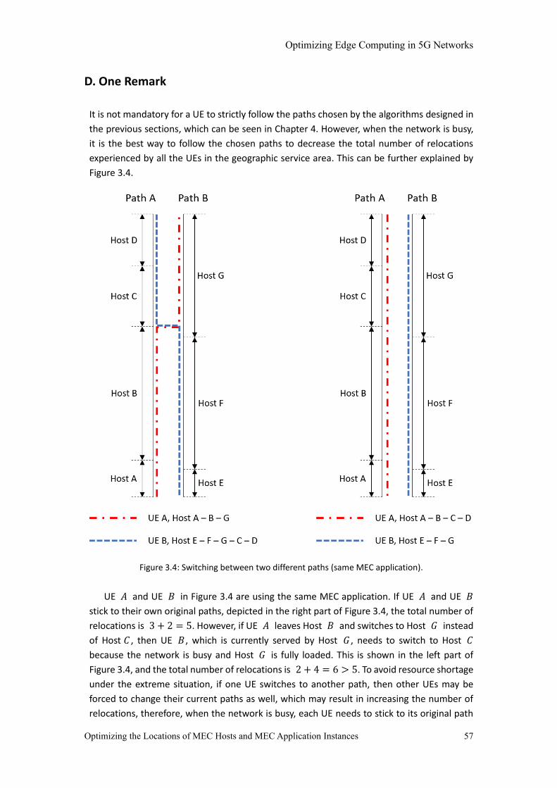
Optimizing Edge Computing in 5G Networks
Optimizing the Locations of MEC Hosts and MEC Application Instances 57
D. One Remark
It is not mandatory for a UE to strictly follow the paths chosen by the algorithms designed in
the previous sections, which can be seen in Chapter 4. However, when the network is busy,
it is the best way to follow the chosen paths to decrease the total number of relocations
experienced by all the UEs in the geographic service area. This can be further explained by
Figure 3.4.
Figure 3.4: Switching between two different paths (same MEC application).
UE 𝐴 and UE 𝐵 in Figure 3.4 are using the same MEC application. If UE 𝐴 and UE 𝐵
stick to their own original paths, depicted in the right part of Figure 3.4, the total number of
relocations is 3 + 2 = 5. However, if UE 𝐴 leaves Host 𝐵 and switches to Host 𝐺 instead
of Host 𝐶 , then UE 𝐵 , which is currently served by Host 𝐺 , needs to switch to Host 𝐶
because the network is busy and Host 𝐺 is fully loaded. This is shown in the left part of
Figure 3.4, and the total number of relocations is 2 + 4 = 6 > 5. To avoid resource shortage
under the extreme situation, if one UE switches to another path, then other UEs may be
forced to change their current paths as well, which may result in increasing the number of
relocations, therefore, when the network is busy, each UE needs to stick to its original path

Optimizing Edge Computing in 5G Networks
Optimizing the Locations of MEC Hosts and MEC Application Instances 58
and avoid switching paths.
However, if the network is not busy and UE 𝐵 can still be served by Host 𝐺, then the
total number of relocations is 2 + 2 = 4 < 5. The scenario where the network is not busy is
further discussed in chapters 4 and 5.
3.5 Tests
Using the algorithms introduced in section 3.3 and 3.4, six locating mechanisms to locate
MEC hosts and MEC applications properly have been generated: greedy + greedy, greedy+
VNS, greedy + multi-KL, simulation-based + greedy, simulation-based + VNS, simulation-
based + multi-KL. In this section, these six locating mechanisms are tested and analyzed.
A. Testing environment
Simulated environments
• Number of sites: 50, 55, 60, 65, 70, 75, 80, 85, 90, 95, 100. The first 50 sites have the
same coverage radius (e.g. 𝑟𝐹 in Figure 3.1) as well as the same distance towards the
road (e.g. |𝑥𝐹| in Figure 3.1), and these sites are uniformly located along the road.
Other sites with different locations and coverage radius are gradually added to the
geographic service area, 5 sites at a time.
• Road length: 126 unit lengths.
• Three types of locations: close to or co-located with gNB-DU, close to or co-located
with gNB-CU, collocated with a UPF which is inside the core network.
• MEC hosts information is shown in Table 3.8. A location No. is used to represent a
location in simulations in this chapter and Chapter 5 for simplicity reason.
Table 3.8: MEC hosts information
Location of MEC hosts Close to gNB-DU Close to gNB-CU Close to 5GC
Location No. 1 2 3
Maximum number of sites one MEC
host can process data from 1 3 5
Maximum amount of available
resources in one MEC host
(computing/storage/processing)
100/100/100 300/300/300 500/500/500
Test the performance of all six locating mechanisms in the simulated geographic service
area described above. Their performance includes the following aspects:
• The total number of relocations (weighted) = number of relocations experienced by
each UE × priority of the MEC application this UE uses.
• The total number of MEC hosts/unit-hosts involved.
• The total amount of resources reserved.
MEC applications
To fully investigate and compare the performance of the six locating mechanisms, three

Optimizing Edge Computing in 5G Networks
Optimizing the Locations of MEC Hosts and MEC Application Instances 59
groups of MEC applications with different settings are used to test the mechanisms. Tables
3.9 - 3.11 show the three different groups separately.
Table 3.9: MEC applications group 1
MEC
APP
Required Resources per UE
(computing/storage/processing) Priority
Acceptable
Locations
Maximum
number of UEs
enter the
geographic
service area
together
1 2/2/6 2 1, 2 3
2 3/3/3 1 1, 2, 3 2
3 2/6/2 2 1, 2, 3 5
4 10/4/3 3 1, 2 2
5 2/8/5 3 1 3
Table 3.10: MEC applications group 2
MEC
APP
Required Resources per UE
(computing/storage/processing) Priority
Acceptable
Locations
Maximum
number of UEs
enter the
geographic service
area together
1 2/2/3 2 1, 2 3
2 3/3/3 1 1, 2, 3 2
3 2/2/3 2 1, 2, 3 5
4 10/4/3 3 1, 2 2
5 2/8/5 3 1 3
Table 3.11: MEC applications group 3
MEC
APP
Required Resources per UE
(computing/storage/processing) Priority
Acceptable
Locations
Maximum number
of UEs enter the
geographic service
area together
1 2/2/3 2 1, 2 3
2 3/3/3 1 1, 2, 3 2
3 2/2/3 3 1, 2, 3 5
4 10/4/3 4 1, 2 2
5 2/8/5 5 1 3
B. Test Results and analysis
Test 1: Test results of MEC application group 1 are shown in Figures 3.5 - 3.8. In the legends
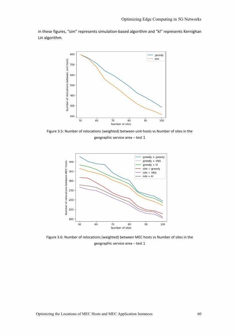
Optimizing Edge Computing in 5G Networks
Optimizing the Locations of MEC Hosts and MEC Application Instances 60
in these figures, “sim” represents simulation-based algorithm and “kl” represents Kernighan
Lin algorithm.
Figure 3.5: Number of relocations (weighted) between unit-hosts vs Number of sites in the
geographic service area – test 1
Figure 3.6: Number of relocations (weighted) between MEC hosts vs Number of sites in the
geographic service area – test 1
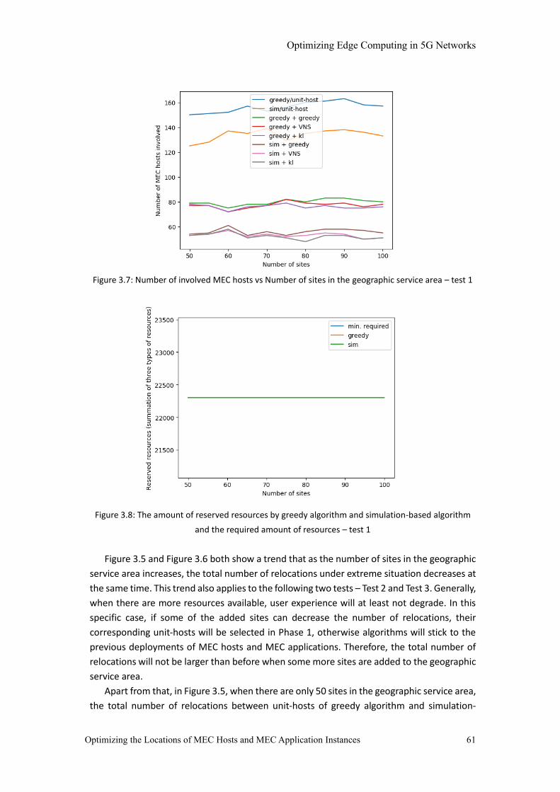
Optimizing Edge Computing in 5G Networks
Optimizing the Locations of MEC Hosts and MEC Application Instances 61
Figure 3.7: Number of involved MEC hosts vs Number of sites in the geographic service area – test 1
Figure 3.8: The amount of reserved resources by greedy algorithm and simulation-based algorithm
and the required amount of resources – test 1
Figure 3.5 and Figure 3.6 both show a trend that as the number of sites in the geographic
service area increases, the total number of relocations under extreme situation decreases at
the same time. This trend also applies to the following two tests – Test 2 and Test 3. Generally,
when there are more resources available, user experience will at least not degrade. In this
specific case, if some of the added sites can decrease the number of relocations, their
corresponding unit-hosts will be selected in Phase 1, otherwise algorithms will stick to the
previous deployments of MEC hosts and MEC applications. Therefore, the total number of
relocations will not be larger than before when some more sites are added to the geographic
service area.
Apart from that, in Figure 3.5, when there are only 50 sites in the geographic service area,
the total number of relocations between unit-hosts of greedy algorithm and simulation-
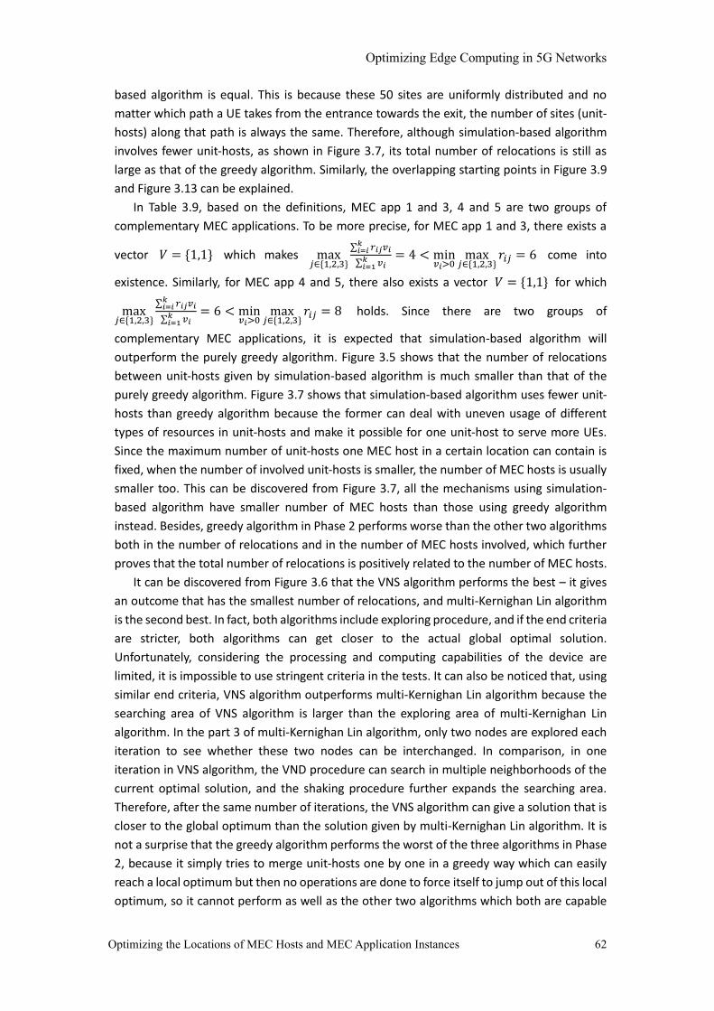
Optimizing Edge Computing in 5G Networks
Optimizing the Locations of MEC Hosts and MEC Application Instances 62
based algorithm is equal. This is because these 50 sites are uniformly distributed and no
matter which path a UE takes from the entrance towards the exit, the number of sites (unit-
hosts) along that path is always the same. Therefore, although simulation-based algorithm
involves fewer unit-hosts, as shown in Figure 3.7, its total number of relocations is still as
large as that of the greedy algorithm. Similarly, the overlapping starting points in Figure 3.9
and Figure 3.13 can be explained.
In Table 3.9, based on the definitions, MEC app 1 and 3, 4 and 5 are two groups of
complementary MEC applications. To be more precise, for MEC app 1 and 3, there exists a
vector 𝑉 = {1,1} which makes max𝑗∈{1,2,3}
∑ 𝑟𝑖𝑗𝑣𝑖𝑘𝑖=𝑖
∑ 𝑣𝑖𝑘𝑖=1
= 4 < min𝑣𝑖>0
max𝑗∈{1,2,3}
𝑟𝑖𝑗 = 6 come into
existence. Similarly, for MEC app 4 and 5, there also exists a vector 𝑉 = {1,1} for which
max𝑗∈{1,2,3}
∑ 𝑟𝑖𝑗𝑣𝑖𝑘𝑖=𝑖
∑ 𝑣𝑖𝑘𝑖=1
= 6 < min𝑣𝑖>0
max𝑗∈{1,2,3}
𝑟𝑖𝑗 = 8 holds. Since there are two groups of
complementary MEC applications, it is expected that simulation-based algorithm will
outperform the purely greedy algorithm. Figure 3.5 shows that the number of relocations
between unit-hosts given by simulation-based algorithm is much smaller than that of the
purely greedy algorithm. Figure 3.7 shows that simulation-based algorithm uses fewer unit-
hosts than greedy algorithm because the former can deal with uneven usage of different
types of resources in unit-hosts and make it possible for one unit-host to serve more UEs.
Since the maximum number of unit-hosts one MEC host in a certain location can contain is
fixed, when the number of involved unit-hosts is smaller, the number of MEC hosts is usually
smaller too. This can be discovered from Figure 3.7, all the mechanisms using simulation-
based algorithm have smaller number of MEC hosts than those using greedy algorithm
instead. Besides, greedy algorithm in Phase 2 performs worse than the other two algorithms
both in the number of relocations and in the number of MEC hosts involved, which further
proves that the total number of relocations is positively related to the number of MEC hosts.
It can be discovered from Figure 3.6 that the VNS algorithm performs the best – it gives
an outcome that has the smallest number of relocations, and multi-Kernighan Lin algorithm
is the second best. In fact, both algorithms include exploring procedure, and if the end criteria
are stricter, both algorithms can get closer to the actual global optimal solution.
Unfortunately, considering the processing and computing capabilities of the device are
limited, it is impossible to use stringent criteria in the tests. It can also be noticed that, using
similar end criteria, VNS algorithm outperforms multi-Kernighan Lin algorithm because the
searching area of VNS algorithm is larger than the exploring area of multi-Kernighan Lin
algorithm. In the part 3 of multi-Kernighan Lin algorithm, only two nodes are explored each
iteration to see whether these two nodes can be interchanged. In comparison, in one
iteration in VNS algorithm, the VND procedure can search in multiple neighborhoods of the
current optimal solution, and the shaking procedure further expands the searching area.
Therefore, after the same number of iterations, the VNS algorithm can give a solution that is
closer to the global optimum than the solution given by multi-Kernighan Lin algorithm. It is
not a surprise that the greedy algorithm performs the worst of the three algorithms in Phase
2, because it simply tries to merge unit-hosts one by one in a greedy way which can easily
reach a local optimum but then no operations are done to force itself to jump out of this local
optimum, so it cannot perform as well as the other two algorithms which both are capable
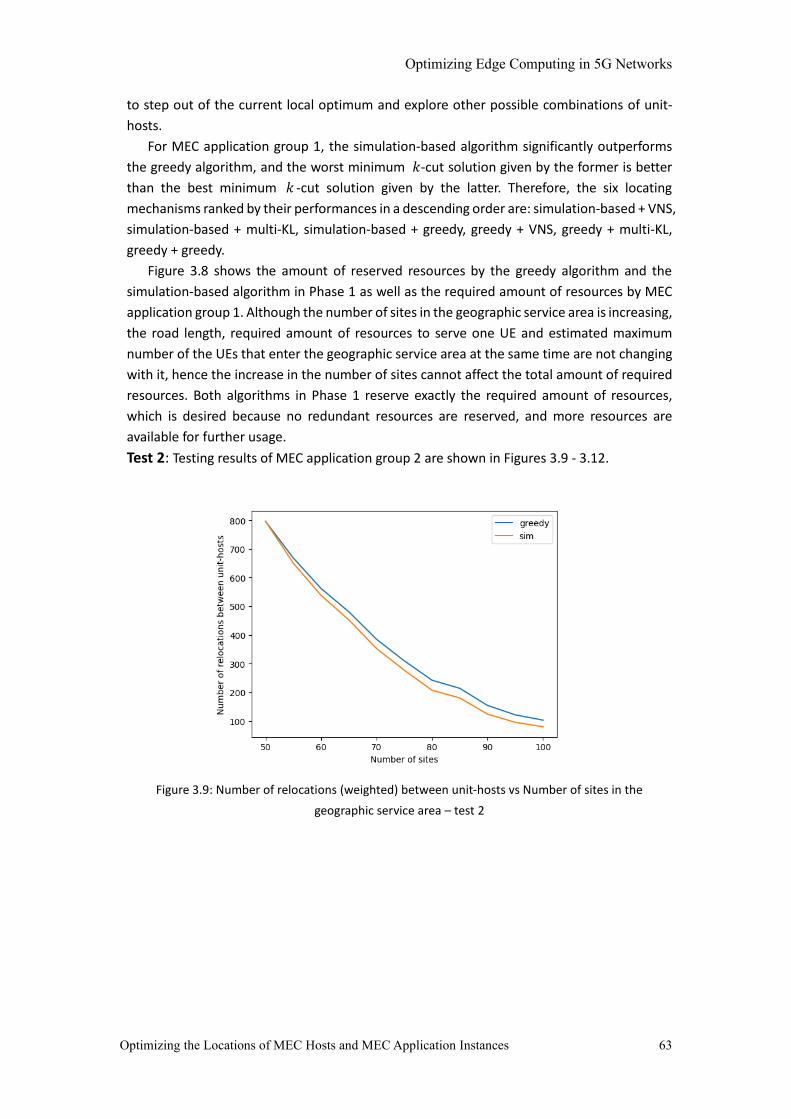
Optimizing Edge Computing in 5G Networks
Optimizing the Locations of MEC Hosts and MEC Application Instances 63
to step out of the current local optimum and explore other possible combinations of unit-
hosts.
For MEC application group 1, the simulation-based algorithm significantly outperforms
the greedy algorithm, and the worst minimum 𝑘-cut solution given by the former is better
than the best minimum 𝑘 -cut solution given by the latter. Therefore, the six locating
mechanisms ranked by their performances in a descending order are: simulation-based + VNS,
simulation-based + multi-KL, simulation-based + greedy, greedy + VNS, greedy + multi-KL,
greedy + greedy.
Figure 3.8 shows the amount of reserved resources by the greedy algorithm and the
simulation-based algorithm in Phase 1 as well as the required amount of resources by MEC
application group 1. Although the number of sites in the geographic service area is increasing,
the road length, required amount of resources to serve one UE and estimated maximum
number of the UEs that enter the geographic service area at the same time are not changing
with it, hence the increase in the number of sites cannot affect the total amount of required
resources. Both algorithms in Phase 1 reserve exactly the required amount of resources,
which is desired because no redundant resources are reserved, and more resources are
available for further usage.
Test 2: Testing results of MEC application group 2 are shown in Figures 3.9 - 3.12.
Figure 3.9: Number of relocations (weighted) between unit-hosts vs Number of sites in the
geographic service area – test 2

Optimizing Edge Computing in 5G Networks
Optimizing the Locations of MEC Hosts and MEC Application Instances 64
Figure 3.10: Number of relocations (weighted) between MEC hosts vs Number of sites in the
geographic service area – test 2
Figure 3.11: Number of involved MEC hosts vs Number of sites in the geographic service area – test 2

Optimizing Edge Computing in 5G Networks
Optimizing the Locations of MEC Hosts and MEC Application Instances 65
Figure 3.12: The amount of reserved resources by greedy algorithm and simulation-based algorithm
and the required amount of resources – test 2
In Figure 3.9, simulation-based algorithm outperforms greedy algorithm, however, if
compared to Figure 3.5, the difference between the outcome of the two algorithms is much
smaller in Figure 3.9 The reason behind is that, in the settings of MEC application group 2,
although MEC applications 1 and 3 are still complementary MEC applications based on the
definition, MEC applications 4 and 5 can no longer complement each other’s resource usages.
This is because both MEC applications 4 and 5 in Table 3.6 have larger required amount of
computing resources than the two other types of resources, hence there does not exist a
vector 𝑉 = {𝑣4, 𝑣5} (𝑣4 > 0, 𝑣5 > 0) , for which the Inequation 3.19 holds. Differences
between the two curves that represent the number of involved unit-hosts in Figure 3.11 are
much smaller than the differences in Figure 3.7 due to the same reason – there is only one
group of complementary MEC applications in Table 3.10, and the advantage of simulation-
based algorithm on high resource efficiency decreases accordingly. Since the number of MEC
hosts is related to the number of selected unit-hosts in Phase 1, differences between curves
that represent the number of MEC hosts in Figure 3.11 are also smaller than the differences
in Figure 3.7. Unsurprisingly, greedy algorithm in Phase 2 gives the highest number of
relocations as well as MEC hosts, and the reason is explained in the analysis of Test 1.
The changes in MEC application settings in Table 3.10 also affect the performances of the
six locating mechanisms. Although the rank of performances of the three graph partitioning
algorithms in Phase 2 remains the same, the difference between the performances of the
two algorithms in Phase 1 is smaller, hence the rank of the six locating mechanisms becomes:
simulation-based + VNS, greedy + VNS, simulation-based + multi-KL, greedy + multi-KL,
simulation-based + greedy, greedy + greedy.
Although the MEC application settings have been changed, both algorithms in Phase 1
can still avoid allocating more resources than needed. The only difference between Figure
3.12 and Figure 3.8 is in the y-axis, since MEC applications group 2 has different requirements
on resources.
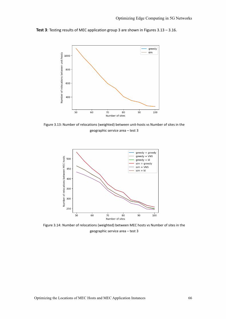
Optimizing Edge Computing in 5G Networks
Optimizing the Locations of MEC Hosts and MEC Application Instances 66
Test 3: Testing results of MEC application group 3 are shown in Figures 3.13 – 3.16.
Figure 3.13: Number of relocations (weighted) between unit-hosts vs Number of sites in the
geographic service area – test 3
Figure 3.14: Number of relocations (weighted) between MEC hosts vs Number of sites in the
geographic service area – test 3

Optimizing Edge Computing in 5G Networks
Optimizing the Locations of MEC Hosts and MEC Application Instances 67
Figure 3.15: Number of involved MEC hosts vs Number of sites in the geographic service area – test 3
Figure 3.16: The amount of reserved resources by greedy algorithm and simulation-based algorithm
and the required amount of resources – test 3
Every MEC application in Table 3.11 has a unique priority, which means that no
complementary MEC applications can be found. Therefore, the performances of the two
algorithms in Phase 1 should be the same. In Figure 3.13, the two curves that represent
number of relocations between unit-hosts using greedy algorithm and simulation-based
algorithm overlap with each other. In Figure 3.15, the numbers of unit-hosts used by the two
algorithms in Phase 1 – greedy and simulation-based algorithms – are equal, and that is the
reason why the four other curves, which represent the numbers of MEC hosts required by
the four different locating mechanisms – greedy + VNS, greedy + Multi-KL, simulation-based
+ VNS and simulation-based + Multi-KL – separately, are closer to each other. Like what has
been discovered in Tests 1 and 2, in Test 3, greedy algorithm in Phase 2 again gives the highest
Optimizing Edge Computing in 5G Networks
Optimizing the Locations of MEC Hosts and MEC Application Instances 68
number of MEC hosts as well as relocations, the reason behind this outcome is explained in
the analysis of Test 1.
The performances of the three algorithms in Phase 2 are still different and the ranking
based on their performances remains unchanged: VNS algorithm ≥ Multi-KL algorithm >
Purely greedy algorithm. The six locating mechanisms ranked by their performances in a
descending order are: simulation-based + VNS and greedy + VNS, simulation-based + multi-
KL and greedy + multi-KL, simulation-based + greedy and greedy + greedy.
The only difference between Table 3.10 and Table 3.11 is the priorities of MEC
applications, which has nothing to do with the two factors – estimated number of UEs that
enter the geographic service area at the same time and the required amount of resources to
serve a UE – that can affect the total amount of required resources. Hence, Figure 3.16 is
exactly the same as Figure 3.12.
C. Conclusions
1. The performance of the algorithms in Phase 1: simulation-based algorithm ≥ purely
greedy algorithm.
2. The performance of the algorithms in Phase 2: VNS algorithm ≥ Multi-KL algorithm >
purely greedy algorithm.
3. When new sites are added to the geographic service area, the number of relocations will
never decrease.
4. The larger the difference min𝑣𝑖>0
max𝑗∈{1,2,3}
𝑟𝑖𝑗 − max𝑗∈{1,2,3}
∑ 𝑟𝑖𝑗𝑣𝑖𝑘𝑖=𝑖
∑ 𝑣𝑖𝑘𝑖=1
is, the better the
performance of the simulation-based algorithm is.
5. If every MEC application has a unique priority, the two algorithms in Phase 1 give the
same outcome.
6. Even though minimizing the number of relocations and the number of MEC hosts
together can be impossible sometimes, at least when the number of relocations has been
minimized, the number of MEC hosts is also small. This means that when the service
continuity is optimized, the O&M costs of MEC hosts also reach a low level.
7. Minimizing the latency and minimizing the total number of relocations cannot be
achieved simultaneously due to the dilemma introduced in section 3.1. In this project,
considering the fact that relocations might cause service interruptions which can
significantly degrade user experience, minimizing the total number of relocations is
chosen as the optimization goal, and the latency requirements of MEC applications
become a constraint.
8. The performances of the six locating mechanisms changes with MEC application settings.
However, no matter how the settings change, mechanism “simulation-based + VNS”
always gives the best outcomes while mechanism “greedy + greedy” always gives the
worst.
9. In Phase 2, greedy algorithm the worst performances but it is the fastest algorithm
among the three and requires the fewest running resources. Due to the fact that this
algorithm is used to determine the deployment of MEC hosts and MEC applications
before the MEC system comes into use, the running time of the algorithm is not an

Optimizing Edge Computing in 5G Networks
Optimizing the Locations of MEC Hosts and MEC Application Instances 69
essential factor. Therefore, heuristic algorithm is a better choice to solve the question in
Phase 2.
3.6. Summary
Chapter 3 mainly answers the four sub-questions of research question 3: Devise an algorithm
to find the optimal location of MEC hosts and the optimal location (MEC host) of a MEC
application.
1. Determine which aspects of MEC applications need to be considered in this master thesis.
Required service latency, required amount of resources and sensitivity to service relocations
are considered. Service latency is the latency between a UE and its serving MEC host. A
certain amount of resources is required to serve a UE using this MEC application. Sensitivity
to service relocations consists of two aspects. One aspect is the service continuity during a
relocation. If a relocation of a MEC application is more likely to cause service interruptions,
then this MEC application has a higher sensitivity to service relocations. Another aspect is,
when service interruption occurs during a relocation, how severe can the consequence be.
The more dangerous the consequence is, the higher the sensitivity of this MEC application to
service interruptions is.
2. How to transform the aspects chosen in sub-question a) into a set of parameters?
The above three aspects are transformed into three parameters. Required service latency
and amount of resources are directly used as two parameters. Sensitivity to service
relocations is transformed into the priority of this MEC application. The higher the sensitivity
is, the higher the priority is.
3. How to locate the MEC hosts as well as MEC applications properly based on these
parameters?
To locate the MEC hosts and MEC applications properly, optimization is needed. The total
number of relocations is selected as the optimization object because service interruptions
during relocations can have bad impacts and, sometimes, threats to lives. Besides, the
number of relocations is positively related to the total number of MEC hosts in the geographic
service area. Therefore, minimizing the total number of relocations can not only limit the
occurrence of unwanted consequences, but also decrease the investments on running and
maintaining MEC hosts. Meanwhile, UEs’ requirements on service latency and resources are
satisfied.
The extreme situation where the number of UEs that in the geographic service area
reaches its maximum value is considered to make sure that the network can handle the worst
situation and always meet UEs’ requirements on resources and service latency. The total
number of relocations is minimized under this extreme situation, using greedy algorithms
and heuristic algorithms.
4. How to test the performance of the algorithms?
The test of algorithms is done by simulations in Python. The five algorithms used in sub-
question c) can form six different locating mechanisms to deploy MEC hosts and MEC
Optimizing Edge Computing in 5G Networks
Optimizing the Locations of MEC Hosts and MEC Application Instances 70
applications. Three tests are designed to test the performance of the six locating mechanisms
under different settings of MEC applications. The outcomes show that, mechanism
“simulation-based + VAS” always gives the smallest number of relocations, as well as a small
number of MEC hosts to be deployed, while mechanism “greedy + greedy” always have the
worst performance among the six locating mechanisms.
Optimizing Edge Computing in 5G Networks
Optimizing the Relocation Process using Reinforcement Learning 71
Chapter 4 Optimizing the Relocation Process
using Reinforcement Learning
Chapter 3 focuses on the extreme situation where the network is fully loaded. When the
network is not busy, a UE can have many options of a target MEC host. These alternatives
come from two aspects:
1. One MEC host is located in a LADN. As mentioned in section 3.1 and section 3.4, any
UE within the serving area of a MEC host can access this MEC host, and it is not necessary for
a UE to follow the paths chosen by the algorithms in Chapter 3, especially when the network
is not busy. Therefore, when a MEC application is assigned with multiple paths, a UE which
uses this MEC application and requires a relocation can be handed over to a MEC host that
has the required MEC application installed but does not belong to the current path of this UE,
hence there might be more than one options of potential target MEC hosts for this UE.
2. The site that one UE is connected to can access MEC hosts in different locations,
some of which may be able to reduce the number of relocations this UE needs to experience.
However, the MEC hosts that reduce the number of relocations may not have the required
MEC application installed. If the UE chooses one of these MEC hosts, the number of
relocations will decrease but one relocation may take longer time because of the extra MEC
application installing procedure.
To find the optimal target MEC host among all the alternatives, research question 4 is
formed into an optimization problem. Traditional reinforcement learning algorithm, SARSA
learning, Deep Q Network (DQN), as well as a newly designed algorithm – quick-start SARSA
learning algorithm are used to solve research question 4.
4.1 Markov Decision Process
A Markov Decision Process (MDP) is a discrete time stochastic control process. It is an
extension of a Markov Chain with multiple actions allowing for choice and rewards used to
indicate the quality of decisions. MDPs are very important in optimizing decision problems,
methodologies like dynamic programming and reinforcement learning need MDPs to solve
optimization problems.
The main components of an MDP are listed below [35]:
1. A set of decision epochs.
Decision epochs are the points in time where decisions are made. In this specific
project, one decision epoch is when a UE needs a relocation. Since the number of
relocations that a UE experiences is limited, the number of decision epochs for a UE
is also limited.
2. A set of system states.
At each decision epoch, the system occupies a state. In this state, a decision needs
to be made to decide which action to be taken. In a Markov Decision Process, there
exist one or more end states. If the system reaches one of these end states, the
current episode ends.
Optimizing Edge Computing in 5G Networks
Optimizing the Relocation Process using Reinforcement Learning 72
3. A set of available actions.
In an MDP model, all actions that can be taken to move from the current state in the
model to a new state are saved in an action set. At each decision epoch, an action
that belongs to this action set should be chosen. After taking the selected action, the
system will reach a new state. If the new state is an end state, then no further actions
will be chosen.
4. A set of state and action dependent immediate rewards.
After the chosen action has been taken, the system will receive an immediate reward.
The reward should reflect the quality of the selected action, hence, in most of the
cases, the reward is related to the action itself. In the context of this master thesis,
the reward is also related to the MEC application type.
5. A set of state and action dependent transition probabilities.
After taking an action, the system will leave its current state and transit to a new
state. Usually, there are multiple potential new states after taking one action, and
the system will reach one of these states following a certain transition probability
distribution. However, in the context of this project, there is only one possible next
state after taking an action, hence the transition probability always equals 1. This
will be further explained in section 4.4.
4.2 Reinforcement Learning
A. Overall Introduction
Reinforcement Learning (RL) is an area of machine learning which is commonly used for
optimizations, and it is one of three basic machine learning paradigms, alongside supervised
learning and unsupervised learning. In reinforcement learning, the software agents should
be able to decide on the actions to take and then attempt to maximize the rewards based on
the feedback from the environment [36].
Compared to supervised learning, reinforcement learning does not need labelled input-
output pairs for training [36]. Instead, the software agents will learn from the environment,
which is usually formulated as an MDP model, by exploring and optimizing itself during the
process. The focus of reinforcement learning is to find a balance between exploration (of
uncharted territory) and exploitation (of current knowledge) [36].
In addition, there are three important terms that need explanations [35]:
1. Decision rules: A decision rule prescribes a procedure for action selection in each
state at a specified decision epoch. There are basically four types of decision rules:
History dependent and Randomized (HR), History dependent and Deterministic (HD),
Markovian and Randomized (MR) and Markovian and Deterministic (MD). The
selection of a target MEC host for a UE is related to its current serving MEC host but
not the MEC hosts previously served this UE. This proves that the system is
Markovian (memoryless). In addition, because reinforcement learning has both
exploration and exploitation aspects, at each decision epoch, either a random action
(randomized) or the current optimal action (deterministic) is selected. Therefore, the
most suitable decision rules for this master thesis are MR and MD.
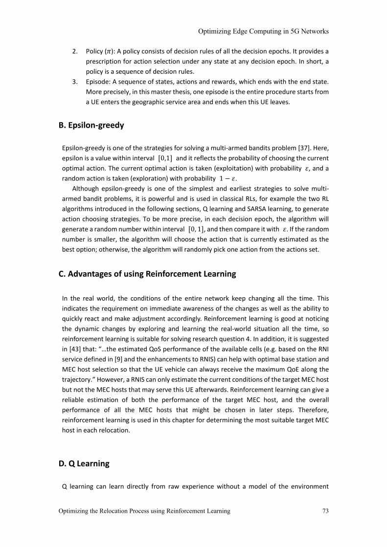
Optimizing Edge Computing in 5G Networks
Optimizing the Relocation Process using Reinforcement Learning 73
2. Policy (𝜋): A policy consists of decision rules of all the decision epochs. It provides a
prescription for action selection under any state at any decision epoch. In short, a
policy is a sequence of decision rules.
3. Episode: A sequence of states, actions and rewards, which ends with the end state.
More precisely, in this master thesis, one episode is the entire procedure starts from
a UE enters the geographic service area and ends when this UE leaves.
B. Epsilon-greedy
Epsilon-greedy is one of the strategies for solving a multi-armed bandits problem [37]. Here,
epsilon is a value within interval [0,1] and it reflects the probability of choosing the current
optimal action. The current optimal action is taken (exploitation) with probability 𝜀, and a
random action is taken (exploration) with probability 1 − 𝜀.
Although epsilon-greedy is one of the simplest and earliest strategies to solve multi-
armed bandit problems, it is powerful and is used in classical RLs, for example the two RL
algorithms introduced in the following sections, Q learning and SARSA learning, to generate
action choosing strategies. To be more precise, in each decision epoch, the algorithm will
generate a random number within interval [0, 1], and then compare it with 𝜀. If the random
number is smaller, the algorithm will choose the action that is currently estimated as the
best option; otherwise, the algorithm will randomly pick one action from the actions set.
C. Advantages of using Reinforcement Learning
In the real world, the conditions of the entire network keep changing all the time. This
indicates the requirement on immediate awareness of the changes as well as the ability to
quickly react and make adjustment accordingly. Reinforcement learning is good at noticing
the dynamic changes by exploring and learning the real-world situation all the time, so
reinforcement learning is suitable for solving research question 4. In addition, it is suggested
in [43] that: “…the estimated QoS performance of the available cells (e.g. based on the RNI
service defined in [9] and the enhancements to RNIS) can help with optimal base station and
MEC host selection so that the UE vehicle can always receive the maximum QoE along the
trajectory.” However, a RNIS can only estimate the current conditions of the target MEC host
but not the MEC hosts that may serve this UE afterwards. Reinforcement learning can give a
reliable estimation of both the performance of the target MEC host, and the overall
performance of all the MEC hosts that might be chosen in later steps. Therefore,
reinforcement learning is used in this chapter for determining the most suitable target MEC
host in each relocation.
D. Q Learning
Q learning can learn directly from raw experience without a model of the environment
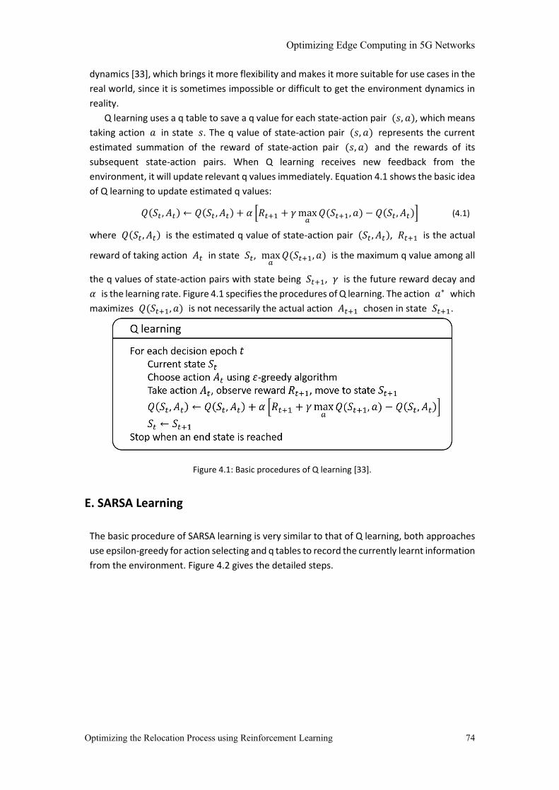
Optimizing Edge Computing in 5G Networks
Optimizing the Relocation Process using Reinforcement Learning 74
dynamics [33], which brings it more flexibility and makes it more suitable for use cases in the
real world, since it is sometimes impossible or difficult to get the environment dynamics in
reality.
Q learning uses a q table to save a q value for each state-action pair (𝑠, 𝑎), which means
taking action 𝑎 in state 𝑠. The q value of state-action pair (𝑠, 𝑎) represents the current
estimated summation of the reward of state-action pair (𝑠, 𝑎) and the rewards of its
subsequent state-action pairs. When Q learning receives new feedback from the
environment, it will update relevant q values immediately. Equation 4.1 shows the basic idea
of Q learning to update estimated q values:
(4.1) 𝑄(𝑆𝑡 , 𝐴𝑡) ← 𝑄(𝑆𝑡 , 𝐴𝑡) + 𝛼 [𝑅𝑡+1 + 𝛾 max
𝑎𝑄(𝑆𝑡+1, 𝑎) − 𝑄(𝑆𝑡, 𝐴𝑡)] (4.1)
where 𝑄(𝑆𝑡 , 𝐴𝑡) is the estimated q value of state-action pair (𝑆𝑡 , 𝐴𝑡), 𝑅𝑡+1 is the actual
reward of taking action 𝐴𝑡 in state 𝑆𝑡, max𝑎
𝑄(𝑆𝑡+1, 𝑎) is the maximum q value among all
the q values of state-action pairs with state being 𝑆𝑡+1, 𝛾 is the future reward decay and
𝛼 is the learning rate. Figure 4.1 specifies the procedures of Q learning. The action 𝑎∗ which
maximizes 𝑄(𝑆𝑡+1, 𝑎) is not necessarily the actual action 𝐴𝑡+1 chosen in state 𝑆𝑡+1.
Figure 4.1: Basic procedures of Q learning [33].
E. SARSA Learning
The basic procedure of SARSA learning is very similar to that of Q learning, both approaches
use epsilon-greedy for action selecting and q tables to record the currently learnt information
from the environment. Figure 4.2 gives the detailed steps.

Optimizing Edge Computing in 5G Networks
Optimizing the Relocation Process using Reinforcement Learning 75
Figure 4.2: Basic procedures of SARSA learning [33].
The major difference between Q learning and SARSA learning is their method to update
q values. The mechanism that SARSA learning uses for updating the q table is shown in
Equation 4.2.
(4.2) 𝑄(𝑆𝑡, 𝐴𝑡) ← 𝑄(𝑆𝑡, 𝐴𝑡) + 𝛼[𝑅𝑡+1 + 𝛾𝑄(𝑆𝑡+1, 𝐴𝑡+1) − 𝑄(𝑆𝑡 , 𝐴𝑡)] (4.2)
where 𝑄(𝑆𝑡 , 𝐴𝑡) is the estimated q value of state-action pair (𝑆𝑡 , 𝐴𝑡), 𝛾 is the future
reward decay and 𝛼 is the learning rate. To accomplish an update in Equation 4.2,
𝑆𝑡, 𝐴𝑡 , 𝑅𝑡+1, 𝑆𝑡+1, 𝐴𝑡+1 are needed, and that is why this algorithm is called “SARSA” learning
algorithm.
A SARSA learning algorithm first selects the action 𝐴𝑡+1, which will be taken in state
𝑆𝑡+1 and then updates 𝑄(𝑆𝑡, 𝐴𝑡) using the q value of state-action pair (𝑆𝑡+1, 𝐴𝑡+1). In
comparison, a Q learning algorithm updates 𝑄(𝑆𝑡 , 𝐴𝑡) with the action 𝑎∗, and this action is
not necessarily the actual action 𝐴𝑡+1 which will be taken in state 𝑆𝑡+1. A reinforcement
algorithm like SARSA learning is called an on-policy reinforcement learning algorithm, and a
reinforcement learning algorithm like Q learning is called an off-policy reinforcement
learning algorithm. Off-policy algorithms can efficiently figure out the optimal policies but it
does not update and evaluate other policies. Therefore off-policy algorithms are more
suitable for agents that do not explore much and stick to the optimal action most of the time.
On-policy algorithms, on the other hand, estimate and update all the policies that are
followed by the agents, including the policies with MR decision rules followed by the agents
that explore. Therefore, compared to off-policy algorithms, on-policy algorithms have a more
comprehensive estimation on the policies and are more suitable for agents that explore. In
this master thesis, agents are UEs, and since the network conditions keep changing, the UEs
need to explore the environment to update the current knowledge of the network at a
reasonable frequency, which makes SARSA learning a better option than Q learning.
4.3 Target MEC host selecting mechanisms
At present, installing MEC applications and instantiating MEC application instances in MEC
hosts is a time-consuming procedure and costs resources in MEC hosts. Therefore, the
deployment of MEC applications needs to be done beforehand following the locating
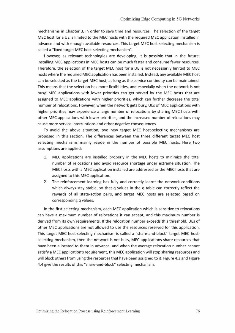
Optimizing Edge Computing in 5G Networks
Optimizing the Relocation Process using Reinforcement Learning 76
mechanisms in Chapter 3, in order to save time and resources. The selection of the target
MEC host for a UE is limited to the MEC hosts with the required MEC application installed in
advance and with enough available resources. This target MEC host selecting mechanism is
called a “fixed target MEC host-selecting mechanism”.
However, as relevant technologies are developing, it is possible that in the future,
installing MEC applications in MEC hosts can be much faster and consume fewer resources.
Therefore, the selection of the target MEC host for a UE is not necessarily limited to MEC
hosts where the required MEC application has been installed. Instead, any available MEC host
can be selected as the target MEC host, as long as the service continuity can be maintained.
This means that the selection has more flexibilities, and especially when the network is not
busy, MEC applications with lower priorities can get served by the MEC hosts that are
assigned to MEC applications with higher priorities, which can further decrease the total
number of relocations. However, when the network gets busy, UEs of MEC applications with
higher priorities may experience a large number of relocations by sharing MEC hosts with
other MEC applications with lower priorities, and the increased number of relocations may
cause more service interruptions and other negative consequences.
To avoid the above situation, two new target MEC host-selecting mechanisms are
proposed in this section. The differences between the three different target MEC host
selecting mechanisms mainly reside in the number of possible MEC hosts. Here two
assumptions are applied:
1. MEC applications are installed properly in the MEC hosts to minimize the total
number of relocations and avoid resource shortage under extreme situation. The
MEC hosts with a MEC application installed are addressed as the MEC hosts that are
assigned to this MEC application.
2. The reinforcement learning has fully and correctly learnt the network conditions
which always stay stable, so that q values in the q table can correctly reflect the
rewards of all state-action pairs, and target MEC hosts are selected based on
corresponding q values.
In the first selecting mechanism, each MEC application which is sensitive to relocations
can have a maximum number of relocations it can accept, and this maximum number is
derived from its own requirements. If the relocation number exceeds this threshold, UEs of
other MEC applications are not allowed to use the resources reserved for this application.
This target MEC host-selecting mechanism is called a “share-and-block” target MEC host-
selecting mechanism, then the network is not busy, MEC applications share resources that
have been allocated to them in advance, and when the average relocation number cannot
satisfy a MEC application’s requirement, this MEC application will stop sharing resources and
will block others from using the resources that have been assigned to it. Figure 4.3 and Figure
4.4 give the results of this “share-and-block” selecting mechanism.
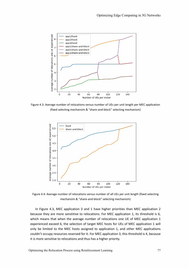
Optimizing Edge Computing in 5G Networks
Optimizing the Relocation Process using Reinforcement Learning 77
Figure 4.3: Average number of relocations versus number of UEs per unit length per MEC application
(fixed selecting mechansim & “share-and-block” selecting mechanism)
Figure 4.4: Average number of relocations versus number of all UEs per unit length (fixed selecting
mechansim & “share-and-block” selecting mechanism)
In Figure 4.3, MEC application 3 and 1 have higher priorities than MEC application 2
because they are more senstitive to relocations. For MEC application 1, its threshold is 6,
which means that when the average number of relocations one UE of MEC application 1
experienced exceed 6, the selection of target MEC hosts for UEs of MEC application 1 will
only be limited to the MEC hosts assigned to application 1, and other MEC applications
couldn’t occupy resources reserved for it. For MEC application 3, this threshold is 4, because
it is more sensitive to relocations and thus has a higher priority.
Optimizing Edge Computing in 5G Networks
Optimizing the Relocation Process using Reinforcement Learning 78
From Figure 4.3, it can be seen that at the very beginning, the average relocation number
of the three MEC application is the same, because they are all using MEC hosts that can
minimize the number of relocations. However, as the number of UEs at the same location of
the road increases, the average number of relocations increase too because the MEC hosts
which have larger coverage are gradually loaded, therefore some of the UEs need to get
served by MEC hosts with smaller coverage and experience more relocations. The average
number of relocations of MEC application 3 is larger than when using the fixed selecting
mechanism, because currently MEC application 3 is sharing its good resources with the other
two MEC applications, whose average numbers of relocations have been lowered. After the
average number of relocation reaches 4, UEs of MEC application 3 will only get served by the
MEC hosts designated to them under extreme situation in Chapter 3. Therefore, the average
number of relocations experienced by UEs of MEC application 3 given by the “share-and-
block” mechanism is first higher than that given by the fixed selecting mechanism, and after
the former reaches 4, these two values become equal. At the same time, the average number
of relocations of MEC applications 1 and 2 increases because some of the resources in MEC
hosts with larger coverage and can provide longer service are reserved for MEC application 3
and cannot be used by others. This time the average number of relocations of MEC
application 1 gets larger than using fixed selecting mechanism because it cannot share better
MEC hosts with MEC application 3 anymore and in the meantime, it has to share its own
assigned MEC hosts with MEC application 2. When the average number of relocations
reaches 6, the same happens to MEC application 1 thus its average number of relocations
decreases and the average number of relocations of MEC application 2 increases rapidly again
and reaches the value given by the fixed selecting mechanism.
The goal of the “share-and-block” mechanism is to mimimize the number of relocations
of all UEs when the network is not busy, under the assumption that installation and
instantiation of a new MEC application (instance) are easy and fast enough. From Figure 4.4
it can be seen that when there are fewer than 120 UEs per unit length, the new mechanism
can reduce the average number of relocations of all the UEs in the geographic service area.
The other new selecting mechanism of target MEC host is called a preemptive target MEC
host-selecting mechanism. When there are multiple UEs requiring a relocation, this selecting
mechanism always starts from selecting MEC hosts for the UEs with the highest priority to
selecting MEC hosts for the UEs with the lowest priority. Therefore, UEs of MEC applications
which are more sensitive to relocations can always get served by the better target MEC hosts.
Figure 4.5 and Figure 4.6 shows the results of preemptive target MEC host-selecting
mechanism.

Optimizing Edge Computing in 5G Networks
Optimizing the Relocation Process using Reinforcement Learning 79
Figure 4.5: Average number of relocations versus number of UEs per unit length per MEC application
(fixed selecting mechansim & preemptive selecting mechanism)
Figure 4.6: Average number of relocations versus number of all UEs per unit length (fixed selecting
mechansim & preemptive selecting mechanism)
In Figure 4.5, the average number of relocations of UEs of MEC application 3 given by
fixed selecting mechanism and preemptive selecting mechanism are the same, because MEC
application 3 has the highest priority among the three applications, its corresponding UEs
can always be served by the best target MEC hosts, and other UEs can only select their own
target MEC hosts later. That is why fixed selecting mechanism and preemptive selecting
mechanism give the same average number of relocations of UEs of MEC application 3, and
the average number of relocations of UEs of a MEC application with higher priority never
Optimizing Edge Computing in 5G Networks
Optimizing the Relocation Process using Reinforcement Learning 80
exceeds that of a MEC application with lower priority. The main difference between these
two mechanisms resides in the average relocation numbers of UEs of MEC application 1 and
2. UEs of these two MEC applications can get served by better MEC hosts as long as these
MEC hosts are still available after the selections performed by the central controller for the
UEs of MEC application 3, and this is not possible in fixed selecting mechanism. Therefore, in
Figure 4.6, the average number of relocations of all UEs using preemptive selecting
mechanism is lower than the average relocation number using fixed selecting mechanism,
only except for the extreme situation - 150 UEs per unit length, where the average number
of relocations of the preemptive selecting mechanism and the fixed selecting mechanism are
the same.
In this section as well as in Chapter 3, only the number of relocations is minimized. In fact,
user experience can be affected by many other factors, such as service latency, service
interruptions and so on. To guarantee an overall satisfied user experience, while selecting
target MEC hosts using the above three mechanisms, these factors can also be taken into
account, like what is done in section 4.4.
4.4 System MDP Model & Assumptions
Relocations (defined in sections 1.1 and 3.1) help with the continuity of MEC services,
however, relocations may also cause problems. For example, if the target MEC host is not
capable to handle the required MEC application instance due to some reasons like no enough
resources, required MEC application not installed, etc., then after relocating the MEC
application to this target MEC host, it is possible that the UE cannot receive required services.
Other possible problems include the latency between the UE and the target MEC host is too
large, the number of relocations afterwards is too large, the relocation takes too much time,
the service failed during the relocation, etc. To achieve the best of each relocation, it is
significant to find a suitable target MEC host, which is addressed in research question 4.
Considering all the aspects mentioned above, four relocation performance indicators are
selected to evaluate the performance of each relocation:
1. The duration time of the relocation
2. Whether there is a service interruption during the relocation
3. The service latency at the target MEC host of the relocation
4. The current available resources in the target MEC host of the relocation
The duration time of relocation is related to the type of MEC application (e.g. dedicated,
stateful, stateless), the transmission delay between the target MEC host and the current
MEC host, the time to install a MEC application, the time to instantiate a MEC application
instance, and the time to set up a PDU Session; service interruption probability is related to
the type of the MEC application and the duration time of a relocation; the service latency
between a UE and the target MEC host is related to the location of this MEC host and the
relevant MEC application type; the current available resources in a MEC host must be
enough to serve the UE, otherwise this MEC host cannot be a potential target MEC host for
this UE. After each relocation, information related to these four performance indicators will
be collected, calculated and sent to the MEC system as the feedback of this relocation.

Optimizing Edge Computing in 5G Networks
Optimizing the Relocation Process using Reinforcement Learning 81
The entire relocation process can be modelled as a Markov Decision Process (MDP). In
this MDP model, 𝑆 is the set of states, each state 𝑠 ∈ 𝑆 represents a MEC host. The end
states in this MDP model are the MEC hosts whose serving areas cover the exit of the road in
the geographic service area. 𝐴𝑠𝑎𝑝𝑝
is the set of all possible actions that can be taken for a
UE, which is now receiving services provided by MEC application 𝑎𝑝𝑝 in MEC host 𝑠 and
needs a relocation. Each action 𝑎 ∈ 𝐴𝑠𝑎𝑝𝑝
is selecting a target MEC host for the UE and
handing the UE over to the selected MEC host. After an action is executed, the UE will move
to a new state/MEC host, with probability 𝑝 = 1. The reward of each action 𝑟𝑒𝑤𝑎𝑟𝑑𝑎 is
derived from the first three performance indicators mentioned above. The reward of each
action is calculated from Equation 4.3:
(4.3) 𝑟𝑒𝑤𝑎𝑟𝑑𝑎 = − 5 × duration time of relocation − 1 (if there is a service
interruption) or 0 (if there is no service interruption) × priority of the MEC
application − 10 × the service latency at the target MEC host selected in
action 𝑎
(4.3)
Assumptions in section 3.1 are still applied in this chapter. Besides, some extra
assumptions are made:
1. All relocation processes are controlled by the central controller, which can be the
MEO or some other system-level functional element in MEC.
2. Installation of MEC applications are costly, both time-wise and resource-wise.
Therefore, it saves time and resources to choose a MEC host which has enough
resources and has required MEC application installed. This target MEC host-selecting
mechanism, which is introduced as “fixed target MEC host-selecting mechanism” in
section 4.3, is the focus in the following sections.
3. In section 1.5, it has been discussed whether to include mobile MEC hosts in this
master thesis or not, and considering the potential increase in the complexity of the
project, mobile MEC hosts are left out and only stationary/fixed MEC hosts are
considered. Relocations can only take place between stationary/fixed MEC hosts.
As explained in section 4.2, SARSA learning algorithm is more suitable for optimizing the
relocation process.
However, considering the fact that the size of the geographic service area has no
limitation, it is possible that the number of MEC hosts in this area is very large, which will
result in a large state space in the system MDP model. Under this circumstance, classical
SARSA learning needs a tremendous big table to save all the q values, and it may take too
much time for searching a required q value in this big q table. Furthermore, when the state
space becomes larger, it takes longer time for the q table to converge. To solve this problem,
a combination of deep learning and SARSA learning, which is called “Deep SARSA” in this
article, is used. The basic idea of “Deep SARSA” comes from Deep Q Network (DQN)
developed by Google DeepMind team [42]. The only difference between these two
algorithms is the same as the difference between SARSA learning and Q learning. The most
outstanding contribution of DQN is that, it uses a neural network to predict the q values,
instead of using a table to save them. By doing this, the size of the state space is not a critical
factor anymore, no matter how big the state space is, the only parameters that need to be
saved and updated are simply the parameters in the deep neural network and the
convergence time will not grow rapidly with the size of the state space.
Optimizing Edge Computing in 5G Networks
Optimizing the Relocation Process using Reinforcement Learning 82
Although introducing a deep neural network into a traditional reinforcement learning
algorithm can help solving the state space explosion problem, it also brings up other
problems. For example, the structure as well as the parameters (e.g. learning rate) of the
deep neural network are crucial to the neural network training and the accuracy of its
prediction. Compared to the straightforward way to save q values in a q table separately,
using a neural network to predict the q values has the impact that different state-action pair
may affect each other, since they share the same deep neural network to do the prediction.
Therefore, the key to increase the accuracy of predictions given by the deep neural network
is that it can find the internal relations between the rewards and the corresponding state-
action pairs and modify the parameters accordingly, which is not easy to achieve since
determining suitable structure of the neural network, activation functions and optimization
function requires experience and lots of experiments. For different environments, their
suitable deep neural networks for prediction can be different.
Since the two algorithms have their own upsides and downsides, in this master thesis,
both are implemented, tested, compared and analyzed. Furthermore, a quick-start SARSA
learning algorithm is designed to combine the advantages of both algorithms. The
performance indicators used to evaluate the algorithms in this chapter include the speed of
convergence and the convergence value. The faster the algorithm converges, the better the
algorithm performs; the higher the convergence value is, the better the algorithm performs.
The choice of algorithm should be based on not only the performance of the algorithm, but
also other factors including the actual scale of the problem, financial requirements, etc.
4.5 Algorithms using Deep SARSA learning
In this section, algorithms for choosing target MEC hosts, updating parameters in deep neural
network, performing reinforcement learning and handling exceptional case are introduced,
each of them is a sub-algorithm of the entire algorithm.
A. Choose target host
To select a suitable target host for each UE, algorithm 6 is designed, and the details are
included in Table 4.1.
Table 4.1: Algorithm 6
Algorithm 6. Choose target host for a UE of application 𝑎𝑝𝑝 in state 𝑠
Input:
𝑀𝐷𝑃: System MDP model
𝑠: The current state this UE is in, that is, the current serving MEC host of this UE
𝑎𝑝𝑝: The application whose instance needs to be moved
𝐷𝑁𝑁𝑝𝑟𝑒𝑑𝑖𝑐𝑡: The deep neural network used to update q values for MEC hosts.
𝜀: The parameter used in 𝜀-greedy algorithm.
𝑃𝑎𝑡ℎ𝑠: 𝑃𝑎𝑡ℎ𝑠(𝑘) records all the paths selected for MEC application 𝑘 and the
number of UEs each path serves.
𝑟𝑒𝑠𝑜𝑢𝑟𝑐𝑒𝑠𝑎𝑝𝑝: The required amount of resources per UE of MEC application 𝑎𝑝𝑝.

Optimizing Edge Computing in 5G Networks
Optimizing the Relocation Process using Reinforcement Learning 83
Output:
𝑎𝑠𝑎𝑝𝑝
: The action taken in state 𝑠 for MEC application 𝑎𝑝𝑝.
𝑠′: Next state/target MEC host
𝑞𝑎𝑝𝑝(𝑠, 𝑎𝑠𝑎𝑝𝑝
): The estimated q value of state-action pair (𝑠, 𝑎𝑠𝑎𝑝𝑝
).
Updated 𝑃𝑎𝑡ℎ𝑠
𝑒 = 𝒓𝒂𝒏𝒅𝒐𝒎𝟏(0,1);
𝑞𝑣𝑎𝑙𝑢𝑒𝑠 = {};
𝐴𝑠𝑎𝑝𝑝
= 𝒈𝒆𝒕_𝒂𝒄𝒕𝒊𝒐𝒏𝒔(𝑀𝐷𝑃, 𝑠, 𝑎𝑝𝑝, 𝑃𝑎𝑡ℎ𝑠);
if 𝑒 ≤ 𝜀 do
for all 𝑎 ∈ 𝐴𝑠𝑎𝑝𝑝
do
𝑞 = 𝐷𝑁𝑁𝑝𝑟𝑒𝑑𝑖𝑐𝑡(𝑠, 𝑎, 𝑎𝑝𝑝);
𝑞𝑣𝑎𝑙𝑢𝑒𝑠 = 𝑞𝑣𝑎𝑙𝑢𝑒𝑠 ∪ {𝑞};
end for
𝑞𝑎𝑝𝑝(𝑠, 𝑎𝑠𝑎𝑝𝑝
), 𝑖𝑛𝑑𝑒𝑥 = 𝑴𝒂𝒙(𝑞𝑣𝑎𝑙𝑢𝑒𝑠);
𝑎𝑠𝑎𝑝𝑝
= 𝐴𝑠𝑎𝑝𝑝
(𝑖𝑛𝑑𝑒𝑥)
else
𝑎𝑠𝑎𝑝𝑝
= 𝒓𝒂𝒏𝒅𝒐𝒎𝟐(𝐴𝑠𝑎𝑝𝑝
);
𝑞𝑎𝑝𝑝(𝑠, 𝑎𝑠𝑎𝑝𝑝
) = 𝐷𝑁𝑁𝑝𝑟𝑒𝑑𝑖𝑐𝑡(𝑠, 𝑎, 𝑎𝑝𝑝);
end if
𝑠′ = 𝑀𝐷𝑃(𝑠, 𝑎𝑠𝑎𝑝𝑝
);
𝑃𝑎𝑡ℎ𝑠 = 𝒓𝒆𝒔𝒆𝒓𝒗𝒆_𝒓𝒆𝒔𝒐𝒖𝒓𝒄𝒆𝒔(𝑃𝑎𝑡ℎ𝑠, 𝑟𝑒𝑠𝑜𝑢𝑟𝑐𝑒𝑠𝑎𝑝𝑝, 𝑠′, 𝑎𝑝𝑝);
To select an action, the first step is to generate a random number between 0 and 1,
function 𝒓𝒂𝒏𝒅𝒐𝒎𝟏(0,1) is used for this purpose. Then, find all possible target MEC hosts
that can be selected, these MEC hosts should have the required MEC application installed,
should have enough resources to serve the UE and should have overlapping serving area with
the current serving MEC host of the UE. Function 𝒈𝒆𝒕_𝒂𝒄𝒕𝒊𝒐𝒏𝒔 is designed to find all the
actions/target MEC hosts that satisfy all the above requirements and return a set 𝐴𝑠𝑎𝑝𝑝
including all the possible options. Its inputs 𝑀𝐷𝑃, 𝑠 and 𝑎𝑝𝑝 are used to find all the MEC
hosts which have overlapping serving area with the current MEC host and have required
application installed, input 𝑃𝑎𝑡ℎ𝑠 is used to check the amount of available resources in each
target MEC host. After getting the possible actions set, compare the generated number e with
epsilon value (𝜀). Based on the result of comparison, different actions will be taken:
If the generated number e is larger than ε, then algorithm will exploit the current
learned q values this time and pick the action 𝑎𝑠𝑎𝑝𝑝
∈ 𝐴𝑠𝑎𝑝𝑝
with the highest q value.
Function 𝑴𝒂𝒙 is used to find the largest value in a set.
If the generated number e is smaller than ε, then algorithm will explore the real
world by randomly selecting a possible action. Function 𝒓𝒂𝒏𝒅𝒐𝒎𝟐 will randomly
pick one element from the input set.
In Deep SARSA learning, q values can be derived from a deep neural network
(𝐷𝑁𝑁𝑝𝑟𝑒𝑑𝑖𝑐𝑡 ). The current state 𝑠 , the selected action 𝑎 and application type 𝑎𝑝𝑝 and
𝐷𝑁𝑁𝑝𝑟𝑒𝑑𝑖𝑐𝑡(𝑠, 𝑎, 𝑎𝑝𝑝) are used to get the predicted q value for state-action pair (𝑠, 𝑎).
After both action 𝑎𝑠𝑎𝑝𝑝
and its corresponding q value 𝑞𝑎𝑝𝑝(𝑠, 𝑎𝑠𝑎𝑝𝑝
) are determined,

Optimizing Edge Computing in 5G Networks
Optimizing the Relocation Process using Reinforcement Learning 84
Algorithm 6 determines the next state/MEC host 𝑠′ in the system MDP model 𝑀𝐷𝑃
according to the selected action 𝑎𝑠𝑎𝑝𝑝
and reserves resources for this UE in the selected
target MEC host 𝑠′ with function 𝑟𝒆𝒔𝒆𝒓𝒗𝒆_𝒓𝒆𝒔𝒐𝒖𝒓𝒄𝒆𝒔.
B. Update parameters of deep neural network
Table 4.2 introduces the approach to update deep neural networks in Deep SARSA Network.
Table 4.2: Algorithm 7
Algorithm 7. Update deep neural networks 𝐷𝑁𝑁𝑝𝑟𝑒𝑑𝑖𝑐𝑡 and 𝐷𝑁𝑁𝑢𝑝𝑑𝑎𝑡𝑒
Input:
𝑠: The current state this UE is in, that is, the current serving MEC host of this
UE.
𝑟𝑒𝑤𝑎𝑟𝑑𝑎𝑠𝑎𝑝𝑝: The reward of taking action 𝑎𝑠
𝑎𝑝𝑝.
𝑎𝑝𝑝: The application whose one instance needs to be moved with the UE.
𝐷𝑁𝑁𝑝𝑟𝑒𝑑𝑖𝑐𝑡: The deep neural network used to update q values for MEC hosts.
𝐷𝑁𝑁𝑡𝑎𝑟𝑔𝑒𝑡: The deep neural network used to provide q values when selecting MEC
hosts.
𝑠′: The next state, or, the selected target MEC host of this UE.
𝑎𝑠𝑎𝑝𝑝
: The action which is selected to be taken at current state.
𝑎𝑠′𝑎𝑝𝑝
: The action which is selected to be taken at next state.
𝛾: Future reward decay.
𝑚𝑒𝑚𝑜𝑟𝑦: A table that saves historical records.
𝑚𝑒𝑚𝑜𝑟𝑦_𝑠𝑖𝑧𝑒: The maximal number of historical records can be saved in table 𝑚𝑒𝑚𝑜𝑟𝑦
for future training.
𝑏𝑎𝑡𝑐ℎ_𝑠𝑖𝑧𝑒: The number of samples utilized in one iteration of training.
𝑝𝑒𝑟𝑖𝑜𝑑: Update period of 𝐷𝑁𝑁𝑢𝑝𝑑𝑎𝑡𝑒.
𝑐𝑜𝑢𝑛𝑡𝑒𝑟: The number of training iterations of 𝐷𝑁𝑁𝑝𝑟𝑒𝑑𝑖𝑐𝑡 after the latest update of
𝐷𝑁𝑁𝑡𝑎𝑟𝑔𝑒𝑡, its initial value is 0.
Output:
Updated 𝐷𝑁𝑁𝑝𝑟𝑒𝑑𝑖𝑐𝑡
Updated 𝐷𝑁𝑁𝑡𝑎𝑟𝑔𝑒𝑡
𝑛𝑒𝑤_𝑟𝑒𝑐𝑜𝑟𝑑 = {𝑠, 𝑎𝑠𝑎𝑝𝑝
, 𝑟𝑒𝑤𝑎𝑟𝑑𝑎𝑠𝑎𝑝𝑝 , 𝑠′, 𝑎𝑠′
𝑎𝑝𝑝};
𝑚𝑒𝑚𝑜𝑟𝑦 = 𝒂𝒅𝒅_𝒓𝒆𝒄𝒐𝒓𝒅(𝑚𝑒𝑚𝑜𝑟𝑦, 𝑛𝑒𝑤_𝑟𝑒𝑐𝑜𝑟𝑑, 𝑚𝑒𝑚𝑜𝑟𝑦_𝑠𝑖𝑧𝑒);
𝑏𝑎𝑡𝑐ℎ = 𝒓𝒂𝒏𝒅𝒐𝒎𝟑(𝑚𝑒𝑚𝑜𝑟𝑦, 𝑏𝑎𝑡𝑐ℎ_𝑠𝑖𝑧𝑒);
for all 𝑟𝑒𝑐𝑜𝑟𝑑 ∈ 𝑏𝑎𝑡𝑐ℎ do
𝑠𝑡𝑎𝑡𝑒 = 𝑟𝑒𝑐𝑜𝑟𝑑(1);
𝑎 = 𝑟𝑒𝑐𝑜𝑟𝑑(2);
𝑟𝑒𝑤𝑎𝑟𝑑 = 𝑟𝑒𝑐𝑜𝑟𝑑(3);
𝑠𝑡𝑎𝑡𝑒′ = 𝑟𝑒𝑐𝑜𝑟𝑑(4);
𝑎′ = 𝑟𝑒𝑐𝑜𝑟𝑑(5);
Optimizing Edge Computing in 5G Networks
Optimizing the Relocation Process using Reinforcement Learning 85
𝑞𝑝𝑟𝑒𝑑𝑖𝑐𝑡 = 𝐷𝑁𝑁𝑝𝑟𝑒𝑑𝑖𝑐𝑡(𝑠𝑡𝑎𝑡𝑒, 𝑎, 𝑎𝑝𝑝);
𝑞𝑡𝑎𝑟𝑔𝑒𝑡 = 𝑟𝑒𝑤𝑎𝑟𝑑 + 𝛾 ∙ 𝐷𝑁𝑁𝑡𝑎𝑟𝑔𝑒𝑡(𝑠𝑡𝑎𝑡𝑒′, 𝑎′, 𝑎𝑝𝑝);
𝐷𝑁𝑁𝑝𝑟𝑒𝑑𝑖𝑐𝑡 = 𝑼𝒑𝒅𝒂𝒕𝒆𝟑(𝐷𝑁𝑁𝑝𝑟𝑒𝑑𝑖𝑐𝑡, 𝑞𝑝𝑟𝑒𝑑𝑖𝑐𝑡, 𝑞𝑡𝑎𝑟𝑔𝑒𝑡);
𝑐𝑜𝑢𝑛𝑡𝑒𝑟 = 𝑐𝑜𝑢𝑛𝑡𝑒𝑟 + 1;
if 𝑐𝑜𝑢𝑛𝑡𝑒𝑟 == 𝑝𝑒𝑟𝑖𝑜𝑑 do
𝑐𝑜𝑢𝑛𝑡𝑒𝑟 = 0
𝐷𝑁𝑁𝑡𝑎𝑟𝑔𝑒𝑡 = 𝐷𝑁𝑁𝑝𝑟𝑒𝑑𝑖𝑐𝑡
end if
end for
To reduce the correlation between two sequential states and their q values, deep SARSA
learning applies two deep neural networks with the same structure but different parameters.
One neural network, or evaluate network (𝐷𝑁𝑁𝑝𝑟𝑒𝑑𝑖𝑐𝑡), is used for learning and providing q
values during action selection, while the other neural network, or target network
(𝐷𝑁𝑁𝑡𝑎𝑟𝑔𝑒𝑡), is used only for estimating the real-world q values. Evaluate network updates
its parameters according to the q values (𝑞𝑡𝑎𝑟𝑔𝑒𝑡) given by the target network, and target
network also updates its parameters to the parameters of evaluate network periodically.
Every time a new record (𝑛𝑒𝑤_𝑟𝑒𝑐𝑜𝑟𝑑) is generated, it will be added to a table (𝑚𝑒𝑚𝑜𝑟𝑦),
if the table is full (the number of records in table 𝑚𝑒𝑚𝑜𝑟𝑦 reaches its maximum size
𝑚𝑒𝑚𝑜𝑟𝑦_𝑠𝑖𝑧𝑒 ), then the oldest record in the table will be removed. Then, 𝑏𝑎𝑡𝑐ℎ_𝑠𝑖𝑧𝑒
number of historical records are randomly picked from 𝑚𝑒𝑚𝑜𝑟𝑦 by function 𝒓𝒂𝒏𝒅𝒐𝒎𝟑.
These records are used to update 𝐷𝑁𝑁𝑝𝑟𝑒𝑑𝑖𝑐𝑡, and function 𝑼𝒑𝒅𝒂𝒕𝒆𝟑 is responsible for
the updates. RMSProp algorithm [40] is the core method to update parameters
in 𝐷𝑁𝑁𝑝𝑟𝑒𝑑𝑖𝑐𝑡 based on the squared difference between 𝑞𝑡𝑎𝑟𝑔𝑒𝑡 and 𝑞𝑝𝑟𝑒𝑑𝑖𝑐𝑡 .
C. Dealing with exception – No MEC hosts currently available
When no MEC host with required MEC application installed has enough resources to serve a
UE, a MEC host that has enough resources should be selected to serve the UE temporarily.
For load-balancing purpose, the MEC host with the largest amount of available resources will
be selected as the temporary MEC host.
Even though this situation is considered, it is not a desired situation of the entire system.
However, due to the uncertainties in the reality, exceptions may occur at any time. To
guarantee service continuity for every UE, Algorithm 8 is introduced, which basic procedure
is shown in Table 4.3.
Table 4.3: Algorithm 8
Algorithm 8. Choose a temporary target MEC host for a UE of MEC application 𝑎𝑝𝑝
Input:
𝑀𝐷𝑃: System MDP model.
𝐿𝐿: A set of all possible locations.
𝑠: The current state this UE is in, that is, the current serving MEC host of this
UE.

Optimizing Edge Computing in 5G Networks
Optimizing the Relocation Process using Reinforcement Learning 86
𝑎𝑝𝑝: The application whose one instance needs to be moved with the UE.
𝑅 = {𝑅𝑙𝑙}, ∀ 𝑙𝑙 ∈ 𝐿𝐿:
𝑅𝑙𝑙 is the set of currently available resources in all unit-hosts in location
𝑙𝑙 ∈ 𝐿𝐿.
𝐺: The directed graph that represents all the sites.
𝑟𝑒𝑠𝑜𝑢𝑟𝑐𝑒𝑠𝑎𝑝𝑝: The required amount of resources per UE of MEC application 𝑎𝑝𝑝.
Output:
Updated 𝑅
𝑠′: The next state of this UE.
𝑠𝑢𝑐𝑐𝑒𝑠𝑠𝑜𝑟𝑠 = 𝒔𝒖𝒄𝒄𝒆𝒔𝒔𝒐𝒓𝒔(𝐺, 𝑠);
𝑚𝑎𝑥_𝑟𝑒𝑠𝑜𝑢𝑟𝑐𝑒𝑠 = 𝑟𝑒𝑠𝑜𝑢𝑟𝑐𝑒𝑠𝑎𝑝𝑝;
𝑚𝑎𝑥_ℎ𝑜𝑠𝑡 = 𝑁𝑜𝑛𝑒;
for all 𝑠𝑢𝑐𝑐𝑒𝑠𝑠𝑜𝑟 ∈ 𝑠𝑢𝑐𝑐𝑒𝑠𝑠𝑜𝑟𝑠 do
for all 𝑙𝑙 ∈ 𝐿𝐿 do
if 𝑅𝑙𝑙(𝑠𝑢𝑐𝑐𝑒𝑠𝑠𝑜𝑟) ≥ 𝑚𝑎𝑥_𝑟𝑒𝑠𝑜𝑢𝑟𝑐𝑒𝑠 do
𝑚𝑎𝑥_ℎ𝑜𝑠𝑡 = 𝑠𝑢𝑐𝑐𝑒𝑠𝑠𝑜𝑟;
𝑚𝑎𝑥_𝑙𝑜𝑐𝑎𝑡𝑖𝑜𝑛 = 𝑙𝑙
end if
end for
end for
𝑠′ = 𝑀𝐷𝑃(𝑚𝑎𝑥ℎ𝑜𝑠𝑡, 𝑚𝑎𝑥𝑙𝑜𝑐𝑎𝑡𝑖𝑜𝑛);
𝑅𝑚𝑎𝑥_𝑙𝑜𝑐𝑎𝑡𝑖𝑜𝑛(𝑚𝑎𝑥_ℎ𝑜𝑠𝑡) = 𝑅𝑚𝑎𝑥_𝑙𝑜𝑐𝑎𝑡𝑖𝑜𝑛(𝑚𝑎𝑥_ℎ𝑜𝑠𝑡) − 𝑟𝑒𝑠𝑜𝑢𝑟𝑐𝑒𝑠𝑎𝑝𝑝;
The basic idea of Algorithm 8 is straightforward: Find all the MEC hosts that have
overlapping serving area with the current serving MEC host of the UE, and this is done by
function 𝒔𝒖𝒄𝒄𝒆𝒔𝒔𝒐𝒓𝒔. Then check current available resources in each MEC host found and
pick the one with the largest amount of available resources as the temporary target MEC host,
install the required MEC application 𝑎𝑝𝑝 on the MEC host and reserve enough resources in
this MEC host. Finally, determine the corresponding state 𝑠′ of this temporary MEC host in
system MDP model 𝑀𝐷𝑃, and state 𝑠′ is UE’s next state in 𝑀𝐷𝑃.
Since this MEC host is temporarily providing MEC application 𝑎𝑝𝑝, after the UE has left
this MEC host, uninstall the MEC application and release all the related resources. Besides,
the rewards/feedback of this MEC host will not be recorded for further training, in case it
affects the performance of 𝐷𝑁𝑁𝑝𝑟𝑒𝑑𝑖𝑐𝑡.
If this exceptional case does not occur frequently, it can be ignored. However, if within a
certain period of time, the number of UEs of MEC application 𝑎𝑝𝑝 that run into this problem
exceeds a certain threshold, which means that the actual number of UEs using 𝑎𝑝𝑝 in the
geographic service area is larger than the estimated number, then scaling up MEC application
𝑎𝑝𝑝 becomes urgent and necessary. In this project, more precisely, if the number of UEs that
need to be served by a temporary MEC host exceeds 10% of the estimated maximum number
of UEs, allocate 30% extra resources for 𝑎𝑝𝑝 in the network.

Optimizing Edge Computing in 5G Networks
Optimizing the Relocation Process using Reinforcement Learning 87
E. Deep SARSA Learning
Algorithm 9 showed in Table 4.4 gives an overall structure of the Deep SARSA learning.
Table 4.4: Algorithm 9
Algorithm 9. Reinforcement learning algorithm related to one UE of MEC
application 𝑎𝑝𝑝
Input:
𝑀𝐷𝑃: System MDP model.
𝑠𝑠𝑡𝑎𝑟𝑡: The starting state of this UE, that is, the first MEC host that serves the UE in
the geographic service area.
𝑎𝑝𝑝: The application whose one instance needs to be moved with the UE.
𝜀: The parameter used in 𝜀-greedy algorithm.
𝑃𝑎𝑡ℎ𝑠: 𝑃𝑎𝑡ℎ𝑠(𝑘) records all the paths selected for MEC application 𝑘 and the
number of UEs each path serves.
𝑟𝑒𝑠𝑜𝑢𝑟𝑐𝑒𝑠𝑎𝑝𝑝: The required amount of resources per UE of MEC application 𝑎𝑝𝑝.
𝐷𝑁𝑁𝑝𝑟𝑒𝑑𝑖𝑐𝑡: The deep neural network used to update q values for MEC hosts.
𝐷𝑁𝑁𝑡𝑎𝑟𝑔𝑒𝑡: The deep neural network used to provide q values when selecting MEC
hosts.
𝑠′: The next state of this UE.
𝛼: Learning rate.
𝛾: Future reward decay.
𝑚𝑒𝑚𝑜𝑟𝑦: A table that saves historical records.
𝑚𝑒𝑚𝑜𝑟𝑦_𝑠𝑖𝑧𝑒: The maximal number of historical records can be saved in table 𝑚𝑒𝑚𝑜𝑟𝑦
for future training.
𝑏𝑎𝑡𝑐ℎ_𝑠𝑖𝑧𝑒: The number of samples utilized in one iteration of training.
𝑝𝑒𝑟𝑖𝑜𝑑: Update period of 𝐷𝑁𝑁𝑢𝑝𝑑𝑎𝑡𝑒.
𝑐𝑜𝑢𝑛𝑡𝑒𝑟: The number of training iterations of 𝐷𝑁𝑁𝑝𝑟𝑒𝑑𝑖𝑐𝑡 after the latest update of
𝐷𝑁𝑁𝑡𝑎𝑟𝑔𝑒𝑡, its initial value is 0.
Output
Updated 𝐷𝑁𝑁𝑝𝑟𝑒𝑑𝑖𝑐𝑡
Updated 𝐷𝑁𝑁𝑡𝑎𝑟𝑔𝑒𝑡
𝑠 = 𝑠𝑠𝑡𝑎𝑟𝑡;
𝑎, 𝑠′, 𝑞, 𝑃𝑎𝑡ℎ𝑠 = 𝑨𝟔(𝑀𝐷𝑃, 𝑠, 𝑎𝑝𝑝, 𝐷𝑁𝑁𝑝𝑟𝑒𝑑𝑖𝑐𝑡 , 𝜀, 𝑃𝑎𝑡ℎ𝑠, 𝑟𝑒𝑠𝑜𝑢𝑟𝑐𝑒𝑠𝑎𝑝𝑝);
While 𝑇𝑟𝑢𝑒 do
𝑂𝑏𝑒𝑟𝑠𝑒𝑟𝑣𝑒 𝑡ℎ𝑒 𝑟𝑒𝑤𝑎𝑟𝑑 𝑜𝑓 𝑡𝑎𝑘𝑖𝑛𝑔 𝑎𝑐𝑡𝑖𝑜𝑛 𝑎 𝑖𝑛 𝑠𝑡𝑎𝑡𝑒 𝑠 ∶ 𝒓𝒆𝒘𝒂𝒓𝒅𝒂;
𝑎′, 𝑠′′, 𝑞′, 𝑃𝑎𝑡ℎ𝑠 = 𝑨𝟔(𝑀𝐷𝑃, 𝑠′, 𝑎𝑝𝑝, 𝐷𝑁𝑁𝑝𝑟𝑒𝑑𝑖𝑐𝑡, 𝜀, 𝑃𝑎𝑡ℎ𝑠, 𝑟𝑒𝑠𝑜𝑢𝑟𝑐𝑒𝑠);
𝐷𝑁𝑁𝑝𝑟𝑒𝑑𝑖𝑐𝑡, 𝐷𝑁𝑁𝑡𝑎𝑟𝑔𝑒𝑡 = 𝑨𝟕(𝑠, 𝑟𝑒𝑤𝑎𝑟𝑑𝑎 , 𝑎𝑝𝑝, 𝐷𝑁𝑁𝑝𝑟𝑒𝑑𝑖𝑐𝑡, 𝐷𝑁𝑁𝑡𝑎𝑟𝑔𝑒𝑡 , 𝑠′, 𝑎, 𝑎′,
𝛾, 𝑚𝑒𝑚𝑜𝑟𝑦, 𝑚𝑒𝑚𝑜𝑟𝑦_𝑠𝑖𝑧𝑒, 𝑏𝑎𝑡𝑐ℎ_𝑠𝑖𝑧𝑒, 𝑝𝑒𝑟𝑖𝑜𝑑, 𝑐𝑜𝑢𝑛𝑡𝑒𝑟)
;
𝐼𝑓 𝑡ℎ𝑒 𝑈𝐸 𝑚𝑜𝑣𝑒𝑠 𝑜𝑢𝑡 𝑜𝑓 𝑡ℎ𝑒 𝑎𝑟𝑒𝑎, 𝑒𝑛𝑑 𝑊ℎ𝑖𝑙𝑒 𝑙𝑜𝑜𝑝
𝑠 = 𝑠′;
𝑎 = 𝑎′;
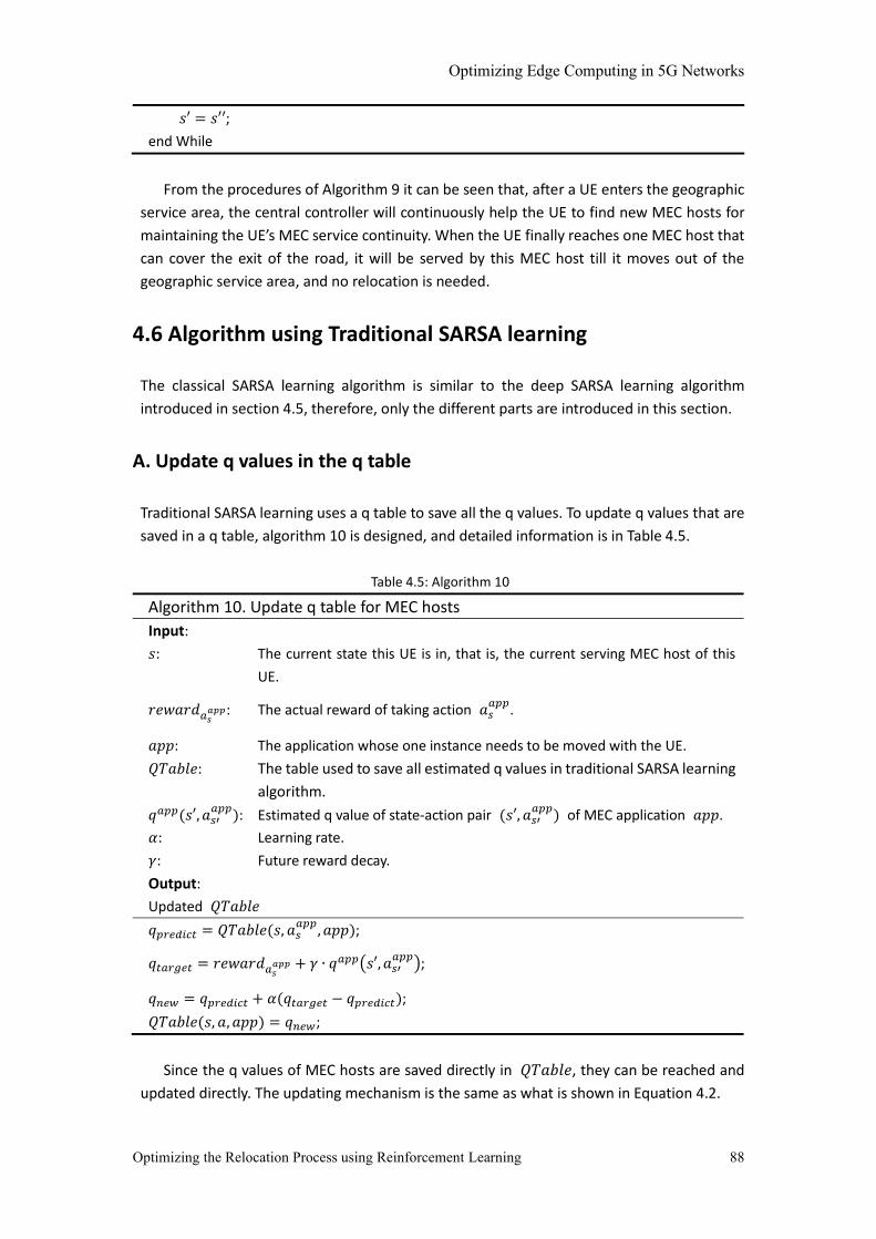
Optimizing Edge Computing in 5G Networks
Optimizing the Relocation Process using Reinforcement Learning 88
𝑠′ = 𝑠′′;
end While
From the procedures of Algorithm 9 it can be seen that, after a UE enters the geographic
service area, the central controller will continuously help the UE to find new MEC hosts for
maintaining the UE’s MEC service continuity. When the UE finally reaches one MEC host that
can cover the exit of the road, it will be served by this MEC host till it moves out of the
geographic service area, and no relocation is needed.
4.6 Algorithm using Traditional SARSA learning
The classical SARSA learning algorithm is similar to the deep SARSA learning algorithm
introduced in section 4.5, therefore, only the different parts are introduced in this section.
A. Update q values in the q table
Traditional SARSA learning uses a q table to save all the q values. To update q values that are
saved in a q table, algorithm 10 is designed, and detailed information is in Table 4.5.
Table 4.5: Algorithm 10
Algorithm 10. Update q table for MEC hosts
Input:
𝑠: The current state this UE is in, that is, the current serving MEC host of this
UE.
𝑟𝑒𝑤𝑎𝑟𝑑𝑎𝑠𝑎𝑝𝑝: The actual reward of taking action 𝑎𝑠
𝑎𝑝𝑝.
𝑎𝑝𝑝: The application whose one instance needs to be moved with the UE.
𝑄𝑇𝑎𝑏𝑙𝑒: The table used to save all estimated q values in traditional SARSA learning
algorithm.
𝑞𝑎𝑝𝑝(𝑠′, 𝑎𝑠′𝑎𝑝𝑝
): Estimated q value of state-action pair (𝑠′, 𝑎𝑠′𝑎𝑝𝑝
) of MEC application 𝑎𝑝𝑝.
𝛼: Learning rate.
𝛾: Future reward decay.
Output:
Updated 𝑄𝑇𝑎𝑏𝑙𝑒
𝑞𝑝𝑟𝑒𝑑𝑖𝑐𝑡 = 𝑄𝑇𝑎𝑏𝑙𝑒(𝑠, 𝑎𝑠𝑎𝑝𝑝
, 𝑎𝑝𝑝);
𝑞𝑡𝑎𝑟𝑔𝑒𝑡 = 𝑟𝑒𝑤𝑎𝑟𝑑𝑎𝑠𝑎𝑝𝑝 + 𝛾 ∙ 𝑞𝑎𝑝𝑝(𝑠′, 𝑎𝑠′
𝑎𝑝𝑝);
𝑞𝑛𝑒𝑤 = 𝑞𝑝𝑟𝑒𝑑𝑖𝑐𝑡 + 𝛼(𝑞𝑡𝑎𝑟𝑔𝑒𝑡 − 𝑞𝑝𝑟𝑒𝑑𝑖𝑐𝑡);
𝑄𝑇𝑎𝑏𝑙𝑒(𝑠, 𝑎, 𝑎𝑝𝑝) = 𝑞𝑛𝑒𝑤;
Since the q values of MEC hosts are saved directly in 𝑄𝑇𝑎𝑏𝑙𝑒, they can be reached and
updated directly. The updating mechanism is the same as what is shown in Equation 4.2.

Optimizing Edge Computing in 5G Networks
Optimizing the Relocation Process using Reinforcement Learning 89
B. Traditional SARSA Learning
Table 4.6 shows the overall structure of the traditional SARSA learning algorithm. Function
𝑨𝟔 is Algorithm 6, and function 𝑨𝟏𝟎 is Algorithm 10.
Table 4.6: SARSA learning algorithm
Algorithm 11. SARSA learning algorithm related to one UE of MEC application 𝑎𝑝𝑝
Input:
𝑀𝐷𝑃: System MDP model.
𝑠𝑠𝑡𝑎𝑟𝑡: The starting state of this UE, that is, the first MEC host that serves the UE in
the geographic service area.
𝑎𝑝𝑝: The application whose one instance needs to be moved with the UE.
𝑄𝑇𝑎𝑏𝑙𝑒: The table used to save all estimated q values in traditional SARSA learning
algorithm.
𝜀: The parameter in 𝜀-greedy algorithm.
𝑃𝑎𝑡ℎ𝑠: 𝑃𝑎𝑡ℎ𝑠(𝑘) records all the paths selected for MEC application 𝑘 and the
number of UEs each path serves.
𝑟𝑒𝑠𝑜𝑢𝑟𝑐𝑒𝑠𝑎𝑝𝑝: The required amount of resources per UE of MEC application 𝑎𝑝𝑝.
𝑠′: The next state of this UE.
𝛼: Learning rate.
𝛾: Future reward decay.
Output
Updated 𝑄𝑇𝑎𝑏𝑙𝑒
𝑠 = 𝑠𝑠𝑡𝑎𝑟𝑡;
𝑎, 𝑠′, 𝑞, 𝑃𝑎𝑡ℎ𝑠 = 𝑨𝟔(𝑀𝐷𝑃, 𝑠, 𝑎𝑝𝑝, 𝑄𝑇𝑎𝑏𝑙𝑒, 𝜀, 𝑃𝑎𝑡ℎ𝑠, 𝑟𝑒𝑠𝑜𝑢𝑟𝑐𝑒𝑠);
While 𝑇𝑟𝑢𝑒 do
𝑂𝑏𝑒𝑟𝑠𝑒𝑟𝑣𝑒 𝑡ℎ𝑒 𝑟𝑒𝑤𝑎𝑟𝑑 𝑜𝑓 𝑡𝑎𝑘𝑖𝑛𝑔 𝑎𝑐𝑡𝑖𝑜𝑛 𝑎 𝑖𝑛 𝑠𝑡𝑎𝑡𝑒 𝑠 ∶ 𝒓𝒆𝒘𝒂𝒓𝒅𝒂;
𝑎′, 𝑠′′, 𝑞′, 𝑃𝑎𝑡ℎ𝑠 = 𝑨𝟔(𝑀𝐷𝑃, 𝑠′, 𝑎𝑝𝑝, 𝑄𝑇𝑎𝑏𝑙𝑒, 𝜀, 𝑃𝑎𝑡ℎ𝑠, 𝑟𝑒𝑠𝑜𝑢𝑟𝑐𝑒𝑠𝑎𝑝𝑝);
𝑄𝑇𝑎𝑏𝑙𝑒 = 𝑨𝟏𝟎(𝑠, 𝑟𝑒𝑤𝑎𝑟𝑑𝑎 , 𝑎𝑝𝑝, 𝑄𝑇𝑎𝑏𝑙𝑒, 𝑞′, 𝛼, 𝛾);
𝐼𝑓 𝑡ℎ𝑒 𝑈𝐸 𝑚𝑜𝑣𝑒𝑠 𝑜𝑢𝑡 𝑜𝑓 𝑡ℎ𝑒 𝑎𝑟𝑒𝑎, 𝑒𝑛𝑑 𝑊ℎ𝑖𝑙𝑒 𝑙𝑜𝑜𝑝
𝑠 = 𝑠′;
𝑎 = 𝑎′;
𝑠′ = 𝑠′′;
end While
4.7 Quick-start SARSA learning algorithm
It has been discussed in section 4.4 that both the deep SARSA algorithm and the traditional
SARSA algorithm have advantages and disadvantages. This can be discovered from Figure 4.7.
The deep neural networks used in the deep SARSA learning algorithm are two identical deep
neural networks with three densely-connected layers each.

Optimizing Edge Computing in 5G Networks
Optimizing the Relocation Process using Reinforcement Learning 90
Figure 4.7: Rewards given by the deep SARSA learning (left) and the traditional SARSA learning (right)
versus episodes
Figure 4.7 is derived from a simulation where the geographic service area contains 1000
sites. One episode starts when a UE enters the geographic service area and ends when it
leaves the area. The reward at each episode is ∑ 𝑟𝑒𝑤𝑎𝑟𝑑𝑎𝑎∈𝐴 , where 𝐴 is a collection of
all the actions taken in this episode, and 𝑟𝑒𝑤𝑎𝑟𝑑𝑎 is calculated from Equation 4.3. The
better the user experience in this episode is, the higher the corresponding reward is.
It can be observed from Figure 4.7 that deep SARSA learning algorithm converges after
about 2500 episodes, and that is much faster than the traditional SARSA learning algorithm,
which converges after 12500 episodes. However, deep SARSA learning algorithm converges
at a lower value than traditional SARSA learning algorithm. The reason behind is explained in
section 4.4.
What is desired is to combine all the advantages of both algorithms and get rid of their
disadvantages. More precisely, the desired algorithm can converge fast and converge at a
high reward. In this section, a quick-start SARSA learning algorithm which is capable to do
both is introduced, and the pseudocode is shown in Table 4.7. Function 𝑨𝟕 is Algorithm 7.
Table 4.7: The quick-start SARSA learning algorithm
Algorithm 12. The quick-start SARSA learning algorithm
Input:
𝑀𝐷𝑃: System MDP model.
𝑠𝑠𝑡𝑎𝑟𝑡: The starting state of this UE, that is, the first MEC host that serves the UE in
the geographic service area.
𝑎𝑝𝑝: The application whose one instance needs to be moved with the UE.
𝑄𝑇𝑎𝑏𝑙𝑒: The table used to save all estimated q values in traditional SARSA
learning algorithm.
𝜀: The parameter in 𝜀-greedy algorithm.
𝑃𝑎𝑡ℎ𝑠: 𝑃𝑎𝑡ℎ𝑠(𝑘) records all the paths selected for MEC application 𝑘 and the
number of UEs each path serves.
𝑟𝑒𝑠𝑜𝑢𝑟𝑐𝑒𝑠𝑎𝑝𝑝: The required amount of resources per UE of MEC application 𝑎𝑝𝑝.
𝑠′: The next state of this UE.
𝛼: Learning rate.

Optimizing Edge Computing in 5G Networks
Optimizing the Relocation Process using Reinforcement Learning 91
𝛾: Future reward decay.
𝐷𝑁𝑁𝑝𝑟𝑒𝑑𝑖𝑐𝑡: The deep neural network used to update q values for MEC hosts.
𝐷𝑁𝑁𝑡𝑎𝑟𝑔𝑒𝑡: The deep neural network used to provide q values when selecting MEC
hosts.
𝑚𝑒𝑚𝑜𝑟𝑦: A table that saves historical records.
𝑚𝑒𝑚𝑜𝑟𝑦_𝑠𝑖𝑧𝑒: The maximal number of historical records can be saved in table 𝑚𝑒𝑚𝑜𝑟𝑦
for future training.
𝑏𝑎𝑡𝑐ℎ_𝑠𝑖𝑧𝑒: The number of samples utilized in one iteration of training.
𝑝𝑒𝑟𝑖𝑜𝑑: Update period of 𝐷𝑁𝑁𝑢𝑝𝑑𝑎𝑡𝑒.
𝑐𝑜𝑢𝑛𝑡𝑒𝑟: The number of training iterations of 𝐷𝑁𝑁𝑝𝑟𝑒𝑑𝑖𝑐𝑡 after the latest update of
𝐷𝑁𝑁𝑡𝑎𝑟𝑔𝑒𝑡, its initial value is 0.
Output
Updated 𝑄𝑇𝑎𝑏𝑙𝑒
Updated 𝐷𝑁𝑁𝑝𝑟𝑒𝑑𝑖𝑐𝑡
Updated 𝐷𝑁𝑁𝑡𝑎𝑟𝑔𝑒𝑡
𝑠 = 𝑠𝑠𝑡𝑎𝑟𝑡;
𝑎, 𝑠′, 𝑞, 𝑃𝑎𝑡ℎ𝑠 = 𝑨𝟔(𝑀𝐷𝑃, 𝑠, 𝑎𝑝𝑝, 𝑄𝑇𝑎𝑏𝑙𝑒, 𝜀, 𝑃𝑎𝑡ℎ𝑠, 𝑟𝑒𝑠𝑜𝑢𝑟𝑐𝑒𝑠𝑎𝑝𝑝);
While 𝑇𝑟𝑢𝑒 do
𝑂𝑏𝑒𝑟𝑠𝑒𝑟𝑣𝑒 𝑡ℎ𝑒 𝑟𝑒𝑤𝑎𝑟𝑑 𝑜𝑓 𝑡𝑎𝑘𝑖𝑛𝑔 𝑎𝑐𝑡𝑖𝑜𝑛 𝑎 𝑖𝑛 𝑠𝑡𝑎𝑡𝑒 𝑠 ∶ 𝒓𝒆𝒘𝒂𝒓𝒅𝒂;
𝑒 = 𝒓𝒂𝒏𝒅𝒐𝒎𝟏(0,1);
𝑞𝑣𝑎𝑙𝑢𝑒𝑠 = {};
𝐴𝑠𝑎𝑝𝑝
= 𝒈𝒆𝒕_𝒂𝒄𝒕𝒊𝒐𝒏𝒔(𝑀𝐷𝑃, 𝑠, 𝑎𝑝𝑝, 𝑃𝑎𝑡ℎ𝑠);
if 𝑒 ≤ 𝜀 do
for all 𝑎 ∈ 𝐴𝑠𝑎𝑝𝑝
do
𝑞 = 𝑄𝑇𝑎𝑏𝑙𝑒(𝑠, 𝑎, 𝑎𝑝𝑝);
if 𝑞 == 0 do
𝑞 = 𝐷𝑁𝑁𝑝𝑟𝑒𝑑𝑖𝑐𝑡(𝑠, 𝑎, 𝑎𝑝𝑝);
end if
𝑞𝑣𝑎𝑙𝑢𝑒𝑠 = 𝑞𝑣𝑎𝑙𝑢𝑒𝑠 ∪ {𝑞};
end for
𝑞𝑎𝑝𝑝(𝑠, 𝑎𝑠𝑎𝑝𝑝
), 𝑖𝑛𝑑𝑒𝑥 = 𝑴𝒂𝒙(𝑞𝑣𝑎𝑙𝑢𝑒𝑠);
𝑎𝑠𝑎𝑝𝑝
= 𝐴𝑠𝑎𝑝𝑝
(𝑖𝑛𝑑𝑒𝑥)
else
𝑎𝑠𝑎𝑝𝑝
= 𝒓𝒂𝒏𝒅𝒐𝒎𝟐(𝐴𝑠𝑎𝑝𝑝
);
𝑞𝑎𝑝𝑝(𝑠, 𝑎𝑠𝑎𝑝𝑝
) = 𝐷𝑁𝑁𝑝𝑟𝑒𝑑𝑖𝑐𝑡(𝑠, 𝑎, 𝑎𝑝𝑝);
end if
𝑠′ = 𝑀𝐷𝑃(𝑠, 𝑎𝑠𝑎𝑝𝑝
, 𝑎𝑝𝑝);
𝑃𝑎𝑡ℎ𝑠 = 𝒓𝒆𝒔𝒆𝒓𝒗𝒆_𝒓𝒆𝒔𝒐𝒖𝒓𝒄𝒆𝒔(𝑃𝑎𝑡ℎ𝑠, 𝑟𝑒𝑠𝑜𝑢𝑟𝑐𝑒𝑠𝑎𝑝𝑝, 𝑠′, 𝑎𝑝𝑝);
𝑄𝑇𝑎𝑏𝑙𝑒 = 𝑨𝟏𝟎(𝑠, 𝑟𝑒𝑤𝑎𝑟𝑑𝑎 , 𝑎𝑝𝑝, 𝑄𝑇𝑎𝑏𝑙𝑒, 𝑞′, 𝛼, 𝛾);
𝐷𝑁𝑁𝑝𝑟𝑒𝑑𝑖𝑐𝑡 , 𝐷𝑁𝑁𝑡𝑎𝑟𝑔𝑒𝑡 = 𝑨𝟕(𝑠, 𝑟𝑒𝑤𝑎𝑟𝑑𝑎 , 𝑎𝑝𝑝, 𝐷𝑁𝑁𝑝𝑟𝑒𝑑𝑖𝑐𝑡, 𝐷𝑁𝑁𝑡𝑎𝑟𝑔𝑒𝑡, 𝑠′, 𝑎, 𝑎′,
𝛾, 𝑚𝑒𝑚𝑜𝑟𝑦, 𝑚𝑒𝑚𝑜𝑟𝑦_𝑠𝑖𝑧𝑒, 𝑏𝑎𝑡𝑐ℎ_𝑠𝑖𝑧𝑒, 𝑝𝑒𝑟𝑖𝑜𝑑, 𝑐𝑜𝑢𝑛𝑡𝑒𝑟);
; 𝐼𝑓 𝑡ℎ𝑒 𝑈𝐸 𝑚𝑜𝑣𝑒𝑠 𝑜𝑢𝑡 𝑜𝑓 𝑡ℎ𝑒 𝑔𝑒𝑜𝑔𝑟𝑎𝑝ℎ𝑖𝑐 𝑠𝑒𝑟𝑣𝑖𝑐𝑒 𝑎𝑟𝑒𝑎, 𝑒𝑛𝑑 𝑊ℎ𝑖𝑙𝑒 𝑙𝑜𝑜𝑝
𝑠 = 𝑠′;
𝑎 = 𝑎′;

Optimizing Edge Computing in 5G Networks
Optimizing the Relocation Process using Reinforcement Learning 92
𝑠′ = 𝑠′′;
end While
The main difference between the quick-start SARSA learning algorithm and the
deep/traditional SARSA learning algorithms lies in the action selection part. if the state-action
pair has not been visited, hence, its corresponding q value in the q table 𝑄𝑇𝑎𝑏𝑙𝑒 still has
the initial value 0, then deep neural network 𝐷𝑁𝑁𝑝𝑟𝑒𝑑𝑖𝑐𝑡 will be used to predict the q value
of this state-action pair. If the state-action pair has been visited before, its corresponding q
value will be provided by the q table 𝑄𝑇𝑎𝑏𝑙𝑒. To make this work, both deep neural networks
𝐷𝑁𝑁𝑝𝑟𝑒𝑑𝑖𝑐𝑡 , 𝐷𝑁𝑁𝑡𝑎𝑟𝑔𝑒𝑡 and the q table 𝑄𝑇𝑎𝑏𝑙𝑒 need to be updated.
Figure 4.8 shows the results given by the quick-start SARSA learning algorithm. The
geographic service area considered here is the same as the geographic service area used in
Figure 4.7.
Figure 4.8: Rewards given by the quick-start SARSA learning algorithm versus episodes
The quick-start SARSA learning algorithm converges after about 2500 episodes, which is
as quick as the deep SARSA learning, and converges at a reward value around -30 which is as
high as the traditional SARSA learning. The reason why this quick-start SARSA learning
algorithm can give a satisfying performance is that it combines prediction in deep SARSA
learning and the q table in traditional SARSA learning. By predicting the reward (q value) of
an unvisited state-action pair using the deep neural network, the convergence of the quick-
start SARSA learning algorithm is faster than the traditional SARSA learning algorithm; and by
saving the updated q value of each visited state-action pair in the q table separately, the
convergence value of the quick-start SARSA learning algorithm is higher than the deep SARSA
learning algorithm.
Although the quick-start SARSA learning algorithm performs well, it is not always
necessary to choose it to solve research problem 4. As mentioned in section 4.4, the choice
of algorithms depends on the actual situation:
1. If the geographic service area is small enough, or, the convergence time of the
Optimizing Edge Computing in 5G Networks
Optimizing the Relocation Process using Reinforcement Learning 93
traditional SARSA learning algorithm is acceptable, then it is redundant to maintain
a deep neural network at the same time, simply using traditional SARSA learning is
the most economical way.
2. If the geographic service area contains (too) many sites and thus requires a huge q
table which is infeasible/costly, or, the convergence value of the deep SARSA learning
algorithm is acceptable, then the deep SARSA learning becomes the best choice since
it can save storage resources and it converges fast.
3. If the geographic service area has a lot of unit-hosts, and the required convergence
speed and convergence value are high, then the quick-start SARSA learning algorithm
is definitely the one to choose.
4.8 Decision-making mechanism
To decide on the group of possible target MEC hosts when an exception takes place, a
decision-making mechanism is proposed in this section. Figure 4.9 illustrates the basic
procedure to determine the possible target MEC hosts following the proposed decision-
making mechanism.
For a MEC application, if the current available MEC hosts with this MEC application
installed are unable to support all the UEs that use this MEC application, but there are still
resources available in other MEC hosts (Exception 1), Algorithm 8 will determine temporary
MEC hosts to serve UEs among these MEC hosts. The required MEC application will be
temporarily installed in the MEC hosts selected by Algorithm 8. If the number of resource
shortage problems of the same MEC application exceeds a certain threshold defined in
section 4.5 (Exception 2), then the “simulation-based + VNS” locating mechanism in Chapter
3 is invoked to allocate more resources for this MEC application.
When the current available MEC hosts in the geographic service area are unable to
support all the UEs (Exception 3), the “simulation-based + VNS” locating mechanism is used
again to properly add more MEC hosts to the network.

Optimizing Edge Computing in 5G Networks
Optimizing the Relocation Process using Reinforcement Learning 94
Figure 4.9: A decision-making mechanism.
4.9 Summary
Chapter 4 mainly answers the first three sub-questions of research question 4: Devise an
algorithm to dynamically find the optimal location of a MEC application processing instance
for a UE (can be all kinds of equipment mounted in vehicles, machines, cellphones, etc.).
a) What parameters of the possible target MEC hosts should be taken into consideration?
Four aspects are considered to estimate the behavior of a possible target MEC host in a
relocation: 1. The duration time of the relocation; 2. Whether there is a service interruption
during the relocation; 3. The latency between the UE and the MEC host; 4. The current
amount of available resources in the MEC host.
The duration time of the relocation and the service latency between the UE and the MEC
host can be directly transformed into two parameters. There is another parameter that
indicates the occurrence of a service interruption during a relocation. If there is no service
interruption, the value of this parameter will be 0 ; otherwise, the value will be 𝑝𝑟𝑖𝑜𝑟𝑘 ,
where 𝑘 is the MEC application required by the UE. The current amount of available
resources inside the MEC host is not transformed into a parameter. Instead, it is used to filter
the MEC hosts that do not have enough resources to serve the UE.
b) How to choose the target MEC host based on these parameters?
The three parameters determined in sub-question a) are weighted and added to each other

Optimizing Edge Computing in 5G Networks
Optimizing the Relocation Process using Reinforcement Learning 95
to evaluate the overall performance of a possible target MEC host in a relocation (as shown
in Equation 4.3). For a UE, not only the performance of its next serving MEC host, but also
the performances of MEC hosts that may serve it afterwards are important. Therefore, an
MDP and reinforcement learning are considered in this sub-question. An MDP is used to
model the network topology and the MEC hosts inside the network. Reinforcement learning
can estimate the overall performances of each possible target MEC host and its subsequential
MEC hosts. Based on the estimations, reinforcement learning algorithms will choose the most
suitable target MEC host for a UE.
c) What information can be provided as feedback after a relocation to estimate the quality
of this relocation and the behavior of the target MEC host? How to process/utilize the
feedback information?
In sub-question b), the most suitable MEC host for a UE is chosen based on the overall
performance of each MEC host estimated by a reinforcement learning algorithm. To estimate
the overall performance, feedback is needed. When a relocation is finished and the UE is
handed over to the target MEC host, the duration of this relocation, the service latency
between the UE and its new MEC host as well as the number of service interruptions in this
relocation will be recorded, calculated and reported to the central controller in which the
reinforcement learning algorithm is implemented. Questions like which entities are
responsible to collect, calculate and transfer the feedback and how the feedback is collected
and calculated are out of the scope of this master thesis.
Every time after receiving the feedback, the reinforcement learning algorithm will first
use the feedback to update its estimations on the overall performance of the relevant MEC
hosts, and then it will decide on the most suitable MEC host for UEs based on the new
estimations.

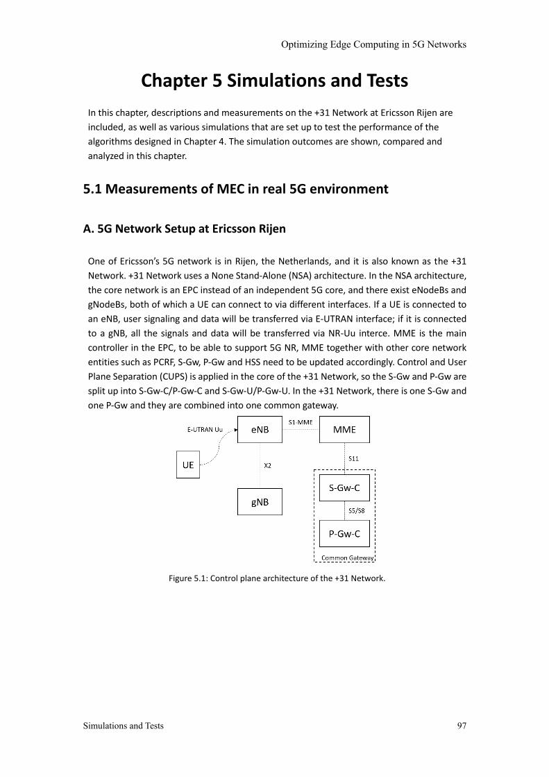
Optimizing Edge Computing in 5G Networks
Simulations and Tests 97
Chapter 5 Simulations and Tests
In this chapter, descriptions and measurements on the +31 Network at Ericsson Rijen are
included, as well as various simulations that are set up to test the performance of the
algorithms designed in Chapter 4. The simulation outcomes are shown, compared and
analyzed in this chapter.
5.1 Measurements of MEC in real 5G environment
A. 5G Network Setup at Ericsson Rijen
One of Ericsson’s 5G network is in Rijen, the Netherlands, and it is also known as the +31
Network. +31 Network uses a None Stand-Alone (NSA) architecture. In the NSA architecture,
the core network is an EPC instead of an independent 5G core, and there exist eNodeBs and
gNodeBs, both of which a UE can connect to via different interfaces. If a UE is connected to
an eNB, user signaling and data will be transferred via E-UTRAN interface; if it is connected
to a gNB, all the signals and data will be transferred via NR-Uu interce. MME is the main
controller in the EPC, to be able to support 5G NR, MME together with other core network
entities such as PCRF, S-Gw, P-Gw and HSS need to be updated accordingly. Control and User
Plane Separation (CUPS) is applied in the core of the +31 Network, so the S-Gw and P-Gw are
split up into S-Gw-C/P-Gw-C and S-Gw-U/P-Gw-U. In the +31 Network, there is one S-Gw and
one P-Gw and they are combined into one common gateway.
Figure 5.1: Control plane architecture of the +31 Network.
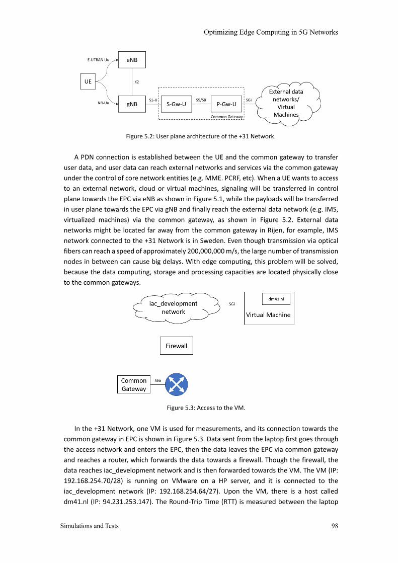
Optimizing Edge Computing in 5G Networks
Simulations and Tests 98
Figure 5.2: User plane architecture of the +31 Network.
A PDN connection is established between the UE and the common gateway to transfer
user data, and user data can reach external networks and services via the common gateway
under the control of core network entities (e.g. MME. PCRF, etc). When a UE wants to access
to an external network, cloud or virtual machines, signaling will be transferred in control
plane towards the EPC via eNB as shown in Figure 5.1, while the payloads will be transferred
in user plane towards the EPC via gNB and finally reach the external data network (e.g. IMS,
virtualized machines) via the common gateway, as shown in Figure 5.2. External data
networks might be located far away from the common gateway in Rijen, for example, IMS
network connected to the +31 Network is in Sweden. Even though transmission via optical
fibers can reach a speed of approximately 200,000,000 m/s, the large number of transmission
nodes in between can cause big delays. With edge computing, this problem will be solved,
because the data computing, storage and processing capacities are located physically close
to the common gateways.
Figure 5.3: Access to the VM.
In the +31 Network, one VM is used for measurements, and its connection towards the
common gateway in EPC is shown in Figure 5.3. Data sent from the laptop first goes through
the access network and enters the EPC, then the data leaves the EPC via common gateway
and reaches a router, which forwards the data towards a firewall. Though the firewall, the
data reaches iac_development network and is then forwarded towards the VM. The VM (IP:
192.168.254.70/28) is running on VMware on a HP server, and it is connected to the
iac_development network (IP: 192.168.254.64/27). Upon the VM, there is a host called
dm41.nl (IP: 94.231.253.147). The Round-Trip Time (RTT) is measured between the laptop

Optimizing Edge Computing in 5G Networks
Simulations and Tests 99
and dm41.nl, and RTT can represent the service latency. Measurement results are used in
simulations in section 5.3 to generate a mechanism for simulating a test environment that is
close to reality.
B. Measurements
The measured RTT between the laptop and host dm41.nl is shown in Figure 5.4. Figure 5.4
contains multiple pings, and the “time” in each record is a RRT, the maximum RRT in Figure
5.4 is 253ms. This dm41.nl host is located close to the core network, and the service latency
can be reduced if the MEC host is located closer to the network edge.

Optimizing Edge Computing in 5G Networks
Simulations and Tests 100
Optimizing Edge Computing in 5G Networks
Simulations and Tests 101
Figure 5.4: The measured RTTs between the laptop and host dm41.nl
5.2 Simulations
A. Assumptions
Before describing the settings of the various simulations in this chapter, the following set of
assumptions is proposed which is applicable to all the simulations in this chapter.
1. All the MEC applications that are provided to the UEs in the geographic service area
are installed in the MEC hosts properly to meet the latency and resource
requirement of every UE under the extreme situation, as what is done in Chapter 3.
This means that, for each MEC application, all the MEC hosts that have it installed
can meet this MEC application’s latency requirement. Therefore, the latency
requirement can be guaranteed by only selecting MEC hosts that have the required
MEC application installed.
2. The only trigger for relocations analyzed in this master thesis is MEC service
discontinuity. When a UE moves out of the coverage of its current serving MEC
host, a new MEC host must be able to serve the UE immediately.
B. Use case
In [20], several end-to-end mobility use cases of MEC have been introduced. Among these
use cases, the use case “prediction of relocation timing” is the most relevant to this thesis
project and will be discussed in this section.
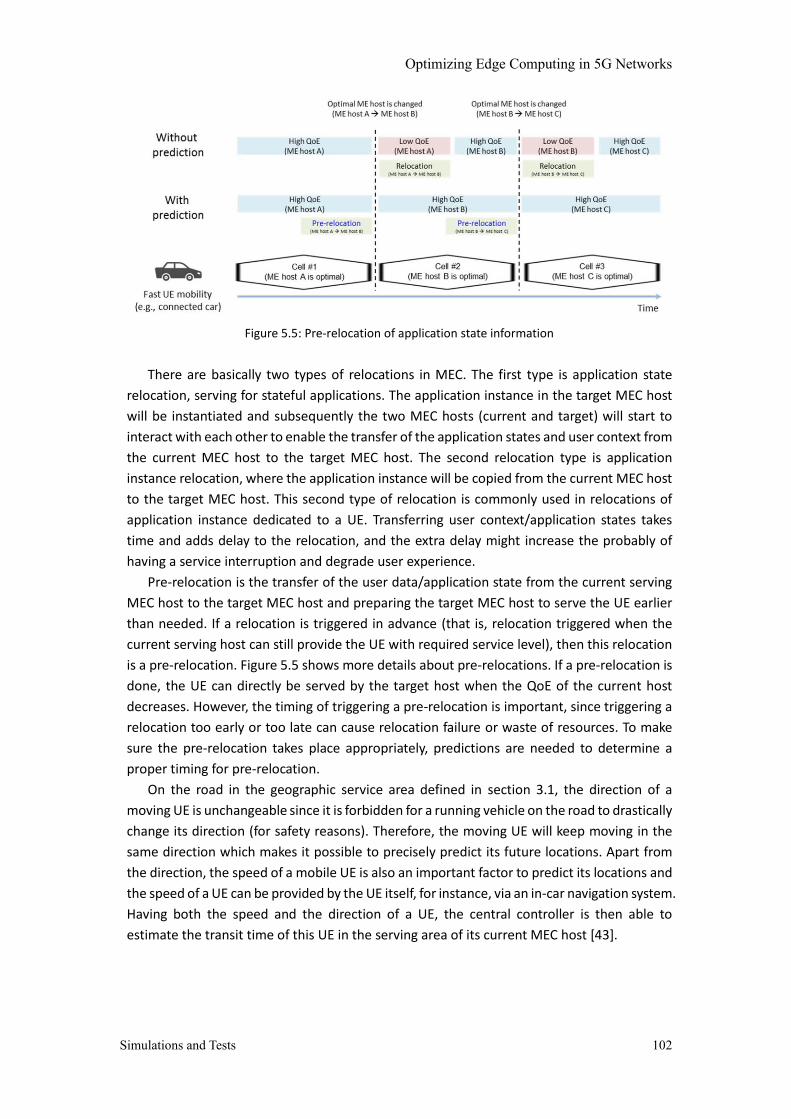
Optimizing Edge Computing in 5G Networks
Simulations and Tests 102
Figure 5.5: Pre-relocation of application state information
There are basically two types of relocations in MEC. The first type is application state
relocation, serving for stateful applications. The application instance in the target MEC host
will be instantiated and subsequently the two MEC hosts (current and target) will start to
interact with each other to enable the transfer of the application states and user context from
the current MEC host to the target MEC host. The second relocation type is application
instance relocation, where the application instance will be copied from the current MEC host
to the target MEC host. This second type of relocation is commonly used in relocations of
application instance dedicated to a UE. Transferring user context/application states takes
time and adds delay to the relocation, and the extra delay might increase the probably of
having a service interruption and degrade user experience.
Pre-relocation is the transfer of the user data/application state from the current serving
MEC host to the target MEC host and preparing the target MEC host to serve the UE earlier
than needed. If a relocation is triggered in advance (that is, relocation triggered when the
current serving host can still provide the UE with required service level), then this relocation
is a pre-relocation. Figure 5.5 shows more details about pre-relocations. If a pre-relocation is
done, the UE can directly be served by the target host when the QoE of the current host
decreases. However, the timing of triggering a pre-relocation is important, since triggering a
relocation too early or too late can cause relocation failure or waste of resources. To make
sure the pre-relocation takes place appropriately, predictions are needed to determine a
proper timing for pre-relocation.
On the road in the geographic service area defined in section 3.1, the direction of a
moving UE is unchangeable since it is forbidden for a running vehicle on the road to drastically
change its direction (for safety reasons). Therefore, the moving UE will keep moving in the
same direction which makes it possible to precisely predict its future locations. Apart from
the direction, the speed of a mobile UE is also an important factor to predict its locations and
the speed of a UE can be provided by the UE itself, for instance, via an in-car navigation system.
Having both the speed and the direction of a UE, the central controller is then able to
estimate the transit time of this UE in the serving area of its current MEC host [43].

Optimizing Edge Computing in 5G Networks
Simulations and Tests 103
C. Prediction
The approach used in this master thesis to predict the timing for pre-relocation is described
as follows:
1. Relocations of different MEC applications have different durations. Considering the
volume of data transferred during relocation, the duration can (usually) be ranked
as stateless < stateful < dedicated. When a UE starts to get served by a new host, its
estimated relocation duration will be determined firstly.
2. The UE will keep reporting its current speed to the central controller and the central
controller will keep tracking its location information by the Location Service (LS)
defined in [32] (for more details, please see Appendix E). More precisely, the central
controller can request the current location of a UE periodically by sending a UE
location Lookup request to the LS or by subscribing to the UE Tracking Subscribe
service.
3. The central controller has the overview of the entire geographic service area, so it
should know the serving area of each MEC host. Otherwise, if supported, the Radio
Node Location Lookup service can be used to retrieve the set of radio nodes that
are currently associated with a MEC host (see more in Appendix E).
4. Every time the central controller receives the location and the speed information of
a UE, it starts to calculate how much time this UE remains in the serving area of its
current MEC host. If the remaining time is short enough, the pre-relocation is
triggered. If supported, another alternative is to make use of the UE Distance
Lookup service in LS by sending a request that includes the UE identity and the
coordinates of the farthest boundary of the serving area of the UE’s current MEC
host to get the distance between UE and the serving area boundary of its current
MEC host.
5. After the pre-relocation is done, the central controller will instruct the UE to
connect to the new MEC host which is timely prepared for its arrival.
To make sure the above approach works properly, the speed of vehicles shouldn’t change
significantly in a very short time, and the reporting and location tracking period should be
short enough. Otherwise, the accuracy of predictions cannot be guaranteed, and may finally
result in fatal consequences.
In [6], another relocation mechanism is introduced. The relocation is triggered by the
serving MEC platform (S-MEP) which is subscribed to RNIS. When a UE crosses a cell boundary
in the underlying network, the RNIS of the serving MEC host (S-RNIS) will notify the cell
change to the S-MEP, and the S-MEP further checks whether the UE has moved out of the
serving area of its serving MEC host. If yes, a relocation will be triggered. When the UE moves
out of the serving area of its source MEC host and the target MEC host is not ready, its user
data will be sent to its source MEC host for processing via the target MEC host. The data
transfer between two MEC hosts takes extra time, and user experience will be degraded
accordingly. This mechanism is not further researched in this master thesis.
Optimizing Edge Computing in 5G Networks
Simulations and Tests 104
5.3 Scenarios & Settings
In this section, three scenarios are designed to test the algorithms in Chapter 4. In addition,
settings of simulations are also introduced.
A. Scenarios
Different scenarios may occur in real world. In this master thesis, three scenarios are
considered:
1. Stable network conditions. The conditions of the network stay stable and the actual
number of UEs is no larger than the estimated number (i.e. no resource shortage
problem). In this scenario, deep SARSA learning algorithm, traditional SARSA
learning algorithm and the quick-start SARSA learning algorithm gradually learn
from the feedback that reflects the network conditions and update their
estimations on the current network conditions.
2. MEC hosts go down. In this scenario, 5% or 25% of the MEC hosts in which MEC
applications are installed go down suddenly. More precisely, this scenario can be
further divided into two sub-scenarios:
a. The sudden defects of MEC hosts are noticed immediately by the network
and the MEC applications installed in these defected MEC hosts are
relocated in other MEC hosts which are still available, possibly instructed
by the MEO.
b. The sudden defects of MEC hosts fail to get noticed by the network, so no
other MEC hosts take the work of the defected MEC hosts, and some of
the UEs might not be able to find suitable MEC hosts. To maintain the
service continuity for every UE, Algorithm 8 should be able to find
temporary MEC hosts when needed, and the central controller will
instruct the chosen temporary MEC hosts to install the required MEC
applications and to instantiate MEC application processing instances. If
the defected MEC hosts are not repaired after some time, locating
mechanism “simulation-based + VNS” should be automatically invoked to
allocate more resources for the MEC applications that face resource
shortage problem in the current available MEC hosts, and to deploy new
MEC hosts in the geographic service area if necessary (as illustrated in
Figure 4.9).
3. Too many UEs. If the geographic service area gets busier than expected, some UEs
may run into problems that no MEC hosts with the required MEC application
installed can serve them anymore. Although there are MEC hosts available to serve
UEs, these MEC hosts have not installed the required MEC application(s) (yet).
According to the decision-making mechanism, a temporary MEC host should be
selected carefully by Algorithm 8 for each UE that couldn’t find an available MEC
host with the required MEC application installed.
Optimizing Edge Computing in 5G Networks
Simulations and Tests 105
B. Settings
Simulated environments
• Number of sites: 800 sites with their axes and coverage radius known in advance,
• Road length: 500 unit lengths
• Locations: co-located with gNB-DU, co-located with gNB-CU, located close to/inside
the core network,
• MEC hosts information is shown in Table 5.1.
Table 5.1: MEC hosts information
Location of MEC hosts Close to gNB-DU Close to gNB-CU Close to 5GC
Location No. 1 2 3
Total number of MEC hosts 168 150 131
Maximum amount of available
resources in one MEC host
(computing/storage/processing)
100/100/100 300/300/300 500/500/500
The approach to simulate the four KPIs to estimate the condition and behavior of a
MEC host is shown below. Because the conditions of network as well as MEC hosts
are dynamic, an indicator may have a range instead of an exact value, and its exact
value will be uniformly and randomly generated from this range.
➢ The duration time of the relocation = time to transfer user context and state
between two MEC hosts (between 0.05-2s) + time to install an MEC application
(between 0-2s) + time to instantiate a MEC application instance (0.005-0.01s) +
time to set up a new PDU Session towards the new MEC host (between 0.01-
0.1s, according to the measurements)
Time to transfer user context and state: The average time to transfer user
context and state of UE of a particular MEC application between a certain
pair of current and target MEC hosts is fixed and the range of the exact time
is 10% of the average.
Time to install an MEC application: This value will be 0 unless a UE has to
choose a MEC host without the required MEC application installed (e.g.
when experiencing resource shortage). In this case, for installing the same
MEC application in different MEC hosts, average installation time is fixed,
and it depends on the MEC application, and the range of the installation
time is 10% of the average; for installing the same MEC application in the
same MEC host, time will not change.
Time to instantiate a MEC application instance: This value is fixed for each
MEC application.
Time to set up a new PDU Session towards the new MEC host: For each
MEC host, the average setup time is fixed and the range of the exact setup
time is 10% of the average.
➢ Whether there is a service interruption during the relocation: During a
relocation of a UE in a simulation, the probably 𝑝 of having one and only one
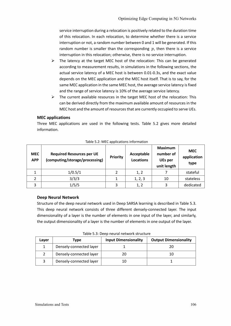
Optimizing Edge Computing in 5G Networks
Simulations and Tests 106
service interruption during a relocation is positively related to the duration time
of this relocation. In each relocation, to determine whether there is a service
interruption or not, a random number between 0 and 1 will be generated. If this
random number is smaller than the corresponding 𝑝, then there is a service
interruption in this relocation; otherwise, there is no service interruption.
➢ The latency at the target MEC host of the relocation: This can be generated
according to measurement results, in simulations in the following sections, the
actual service latency of a MEC host is between 0.01-0.3s, and the exact value
depends on the MEC application and the MEC host itself. That is to say, for the
same MEC application in the same MEC host, the average service latency is fixed
and the range of service latency is 10% of the average service latency.
➢ The current available resources in the target MEC host of the relocation: This
can be derived directly from the maximum available amount of resources in the
MEC host and the amount of resources that are currently occupied to serve UEs.
MEC applications
Three MEC applications are used in the following tests. Table 5.2 gives more detailed
information.
Table 5.2: MEC applications information
MEC
APP
Required Resources per UE
(computing/storage/processing) Priority
Acceptable
Locations
Maximum
number of
UEs per
unit length
MEC
application
type
1 1/0.5/1 2 1, 2 7 stateful
2 3/3/3 1 1, 2, 3 10 stateless
3 1/5/5 3 1, 2 3 dedicated
Deep Neural Network
Structure of the deep neural network used in Deep SARSA learning is described in Table 5.3.
This deep neural network consists of three different densely-connected layer. The input
dimensionality of a layer is the number of elements in one input of the layer, and similarly,
the output dimensionality of a layer is the number of elements in one output of the layer.
Table 5.3: Deep neural network structure
Layer Type Input Dimensionality Output Dimensionality
1 Densely-connected layer 1 20
2 Densely-connected layer 20 10
3 Densely-connected layer 10 1
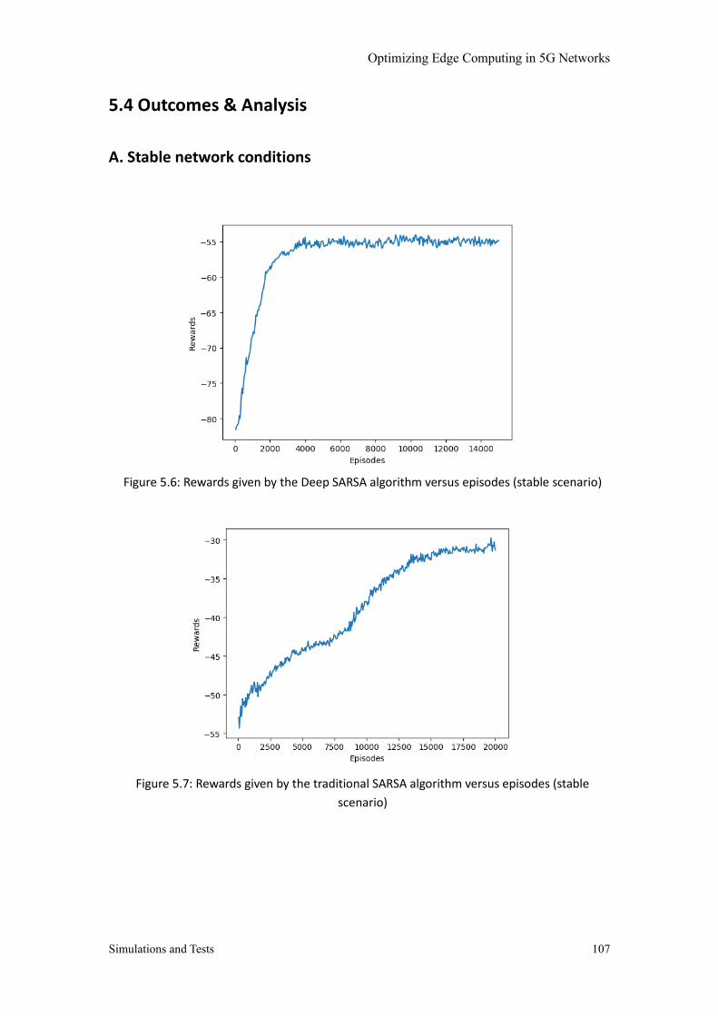
Optimizing Edge Computing in 5G Networks
Simulations and Tests 107
5.4 Outcomes & Analysis
A. Stable network conditions
Figure 5.6: Rewards given by the Deep SARSA algorithm versus episodes (stable scenario)
Figure 5.7: Rewards given by the traditional SARSA algorithm versus episodes (stable
scenario)
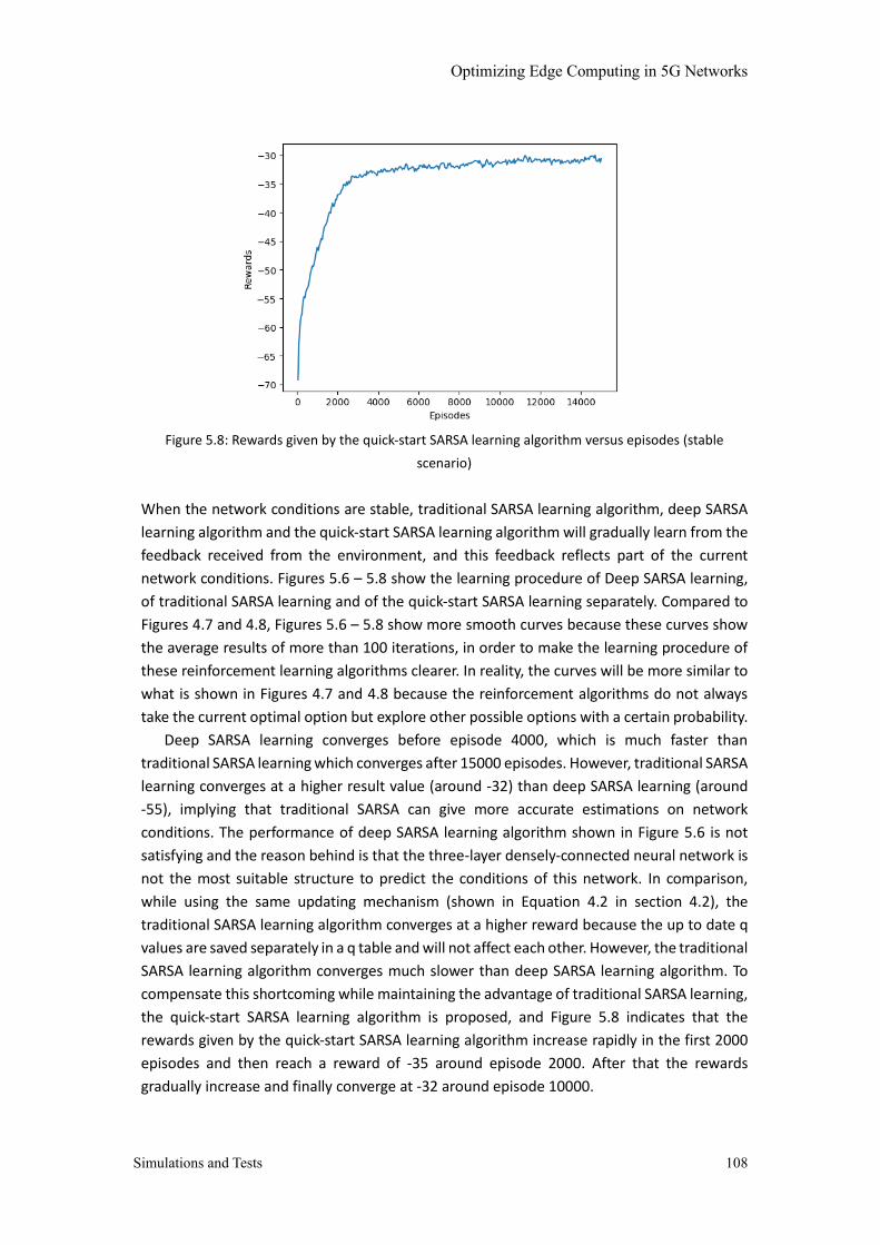
Optimizing Edge Computing in 5G Networks
Simulations and Tests 108
Figure 5.8: Rewards given by the quick-start SARSA learning algorithm versus episodes (stable
scenario)
When the network conditions are stable, traditional SARSA learning algorithm, deep SARSA
learning algorithm and the quick-start SARSA learning algorithm will gradually learn from the
feedback received from the environment, and this feedback reflects part of the current
network conditions. Figures 5.6 – 5.8 show the learning procedure of Deep SARSA learning,
of traditional SARSA learning and of the quick-start SARSA learning separately. Compared to
Figures 4.7 and 4.8, Figures 5.6 – 5.8 show more smooth curves because these curves show
the average results of more than 100 iterations, in order to make the learning procedure of
these reinforcement learning algorithms clearer. In reality, the curves will be more similar to
what is shown in Figures 4.7 and 4.8 because the reinforcement algorithms do not always
take the current optimal option but explore other possible options with a certain probability.
Deep SARSA learning converges before episode 4000, which is much faster than
traditional SARSA learning which converges after 15000 episodes. However, traditional SARSA
learning converges at a higher result value (around -32) than deep SARSA learning (around
-55), implying that traditional SARSA can give more accurate estimations on network
conditions. The performance of deep SARSA learning algorithm shown in Figure 5.6 is not
satisfying and the reason behind is that the three-layer densely-connected neural network is
not the most suitable structure to predict the conditions of this network. In comparison,
while using the same updating mechanism (shown in Equation 4.2 in section 4.2), the
traditional SARSA learning algorithm converges at a higher reward because the up to date q
values are saved separately in a q table and will not affect each other. However, the traditional
SARSA learning algorithm converges much slower than deep SARSA learning algorithm. To
compensate this shortcoming while maintaining the advantage of traditional SARSA learning,
the quick-start SARSA learning algorithm is proposed, and Figure 5.8 indicates that the
rewards given by the quick-start SARSA learning algorithm increase rapidly in the first 2000
episodes and then reach a reward of -35 around episode 2000. After that the rewards
gradually increase and finally converge at -32 around episode 10000.
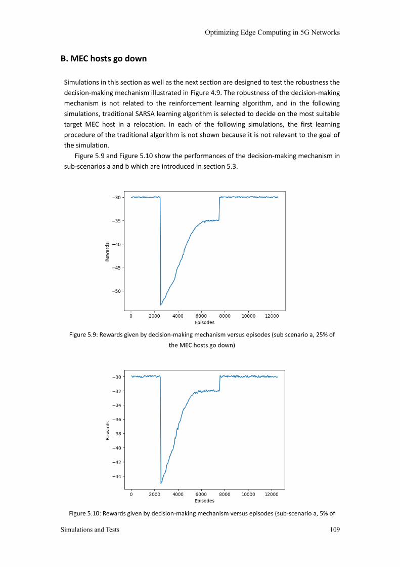
Optimizing Edge Computing in 5G Networks
Simulations and Tests 109
B. MEC hosts go down
Simulations in this section as well as the next section are designed to test the robustness the
decision-making mechanism illustrated in Figure 4.9. The robustness of the decision-making
mechanism is not related to the reinforcement learning algorithm, and in the following
simulations, traditional SARSA learning algorithm is selected to decide on the most suitable
target MEC host in a relocation. In each of the following simulations, the first learning
procedure of the traditional algorithm is not shown because it is not relevant to the goal of
the simulation.
Figure 5.9 and Figure 5.10 show the performances of the decision-making mechanism in
sub-scenarios a and b which are introduced in section 5.3.
Figure 5.9: Rewards given by decision-making mechanism versus episodes (sub scenario a, 25% of
the MEC hosts go down)
Figure 5.10: Rewards given by decision-making mechanism versus episodes (sub-scenario a, 5% of
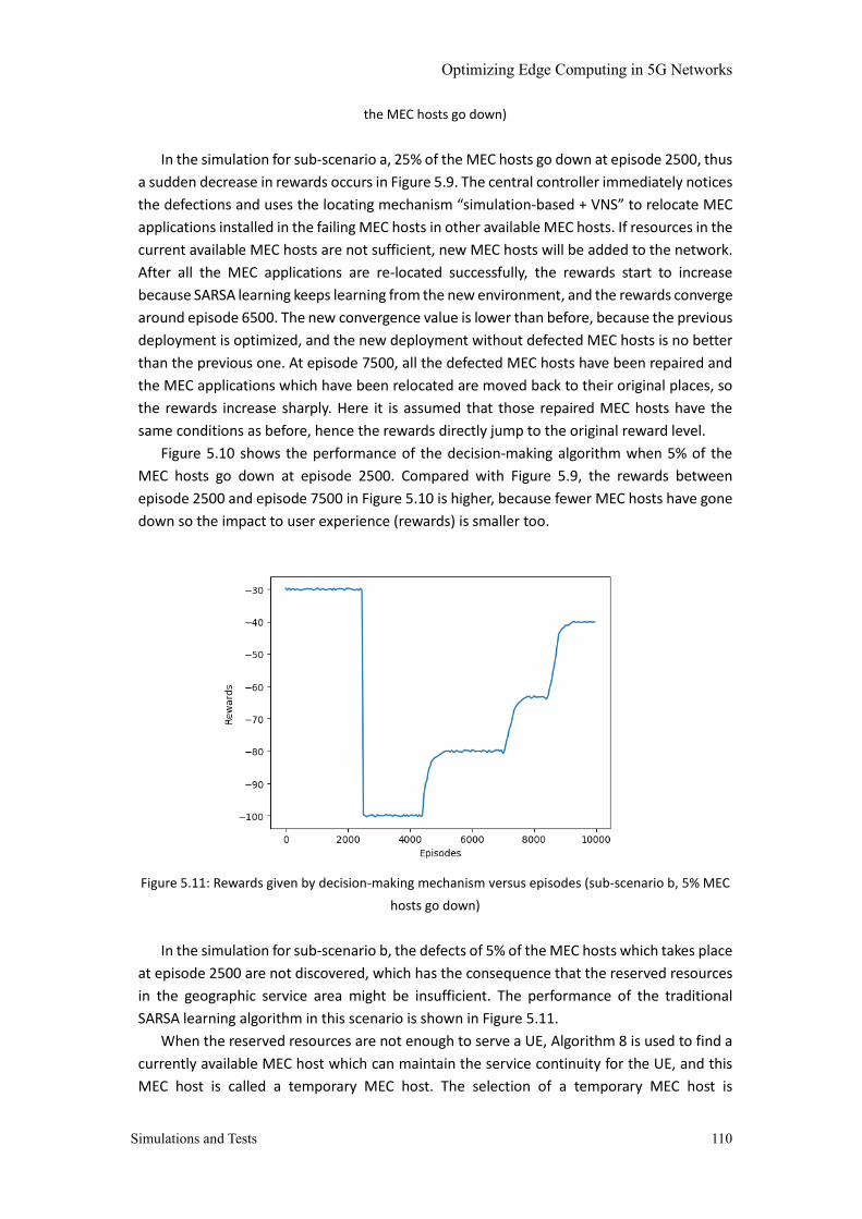
Optimizing Edge Computing in 5G Networks
Simulations and Tests 110
the MEC hosts go down)
In the simulation for sub-scenario a, 25% of the MEC hosts go down at episode 2500, thus
a sudden decrease in rewards occurs in Figure 5.9. The central controller immediately notices
the defections and uses the locating mechanism “simulation-based + VNS” to relocate MEC
applications installed in the failing MEC hosts in other available MEC hosts. If resources in the
current available MEC hosts are not sufficient, new MEC hosts will be added to the network.
After all the MEC applications are re-located successfully, the rewards start to increase
because SARSA learning keeps learning from the new environment, and the rewards converge
around episode 6500. The new convergence value is lower than before, because the previous
deployment is optimized, and the new deployment without defected MEC hosts is no better
than the previous one. At episode 7500, all the defected MEC hosts have been repaired and
the MEC applications which have been relocated are moved back to their original places, so
the rewards increase sharply. Here it is assumed that those repaired MEC hosts have the
same conditions as before, hence the rewards directly jump to the original reward level.
Figure 5.10 shows the performance of the decision-making algorithm when 5% of the
MEC hosts go down at episode 2500. Compared with Figure 5.9, the rewards between
episode 2500 and episode 7500 in Figure 5.10 is higher, because fewer MEC hosts have gone
down so the impact to user experience (rewards) is smaller too.
Figure 5.11: Rewards given by decision-making mechanism versus episodes (sub-scenario b, 5% MEC
hosts go down)
In the simulation for sub-scenario b, the defects of 5% of the MEC hosts which takes place
at episode 2500 are not discovered, which has the consequence that the reserved resources
in the geographic service area might be insufficient. The performance of the traditional
SARSA learning algorithm in this scenario is shown in Figure 5.11.
When the reserved resources are not enough to serve a UE, Algorithm 8 is used to find a
currently available MEC host which can maintain the service continuity for the UE, and this
MEC host is called a temporary MEC host. The selection of a temporary MEC host is

Optimizing Edge Computing in 5G Networks
Simulations and Tests 111
introduced in Table 4.3. According to the decision-making mechanism, more resources will
be allocated for a MEC application when the number of resource-insufficient cases of this
MEC application reaches a certain threshold (detailed information can be found in section
4.5). This is the reason why the rewards increase three times after the degradation – different
MEC applications have different thresholds, once extra resources have been allocated for a
MEC application, the rewards will increase because these new resources are carefully
allocated to enhance the rewards. After about 8500 episodes, enough resources have been
allocated to all the three MEC applications, but the rewards are lower than the original level
because of the defected MEC hosts.
C. Too many UEs
In the simulation for this scenario, the network stays stable and every MEC host works
properly. However, the number of UEs in the geographic service area is more than expected
so resources allocated by the locating mechanism designed in Chapter 3 are not enough
anymore. Under this situation, the decision-making mechanism should be able to assign UEs
to temporary MEC hosts, and allocate more resources if needed. Figure 5.12 shows the
performances of the decision-making mechanism in case too many UEs are present in the
geographic service area.
Figure 5.12: Rewards given by decision-making mechanism versus episodes (Too many UEs)
The total number of UEs within in the geographic service area gradually increases after
episode 900 and then stays stable after another 800 episodes, hence in Figure 5.12, the
rewards gradually decrease between episode 900 and episode 1700. When all of the reserved
resources have been used, temporary MEC hosts are selected, which further decrease the
rewards. Fortunately, around episode 2800, the number of resource-insufficient cases
reaches the threshold to trigger the locating mechanism “simulation-based + VNS” algorithm
to start to allocate extra resources, after which the rewards increase again. After extra
resources are allocated, the rewards converge at a lower level than before because there are

Optimizing Edge Computing in 5G Networks
Simulations and Tests 112
more UEs in the geographic service area so the overall user experience degrades.
D. Average number of relocations versus the number of UEs in the
geographic service area
Generally, if there are more UEs in the geographic service area, the average user experience
will degrade, or at least remain unchanged. This is further proved in this section. Figure 5.13
shows the average number of relocations one UE experiences when there are different
numbers of UEs per unit length in the geographic service area. Figure 5.13 shows a clear trend:
when the number of UEs per unit length increases, the average number of relocations that
one UE experiences increases at the same time. The reason behind this trend is that, when
the network is busy, MEC hosts with larger serving area can be fully loaded. Therefore, some
of the UEs are served by MEC hosts with smaller serving area instead, which increases the
number of relocations.
It is also shown in Figure 5.13 that no matter how many UEs are in the geographic service
area, as long as the reserved resources are enough, the average number of relocations of one
UE of a MEC application with a higher priority (e.g. MEC application 3) can hardly exceed that
of a MEC application with a lower priority (e.g. MEC application 2). This is partially because
of the basic rule in section 3.3, and another reason is that, relocations related to MEC
applications with higher priorities have more effects on the weighted number of relocations
( 𝑅𝑊 ), therefore, to minimize 𝑅𝑊 , eliminating the relocations (between unit-hosts)
experienced by the UEs that are using MEC applications with higher priorities is more
effective.
Figure 5.13: Average number of relocations experienced by a UE versus the number of UEs per unit
length within the geographic service area
Optimizing Edge Computing in 5G Networks
Simulations and Tests 113
5.5 Summary
In this chapter, the Non-Stand Alone (NSA) architecture of the Ericsson +31 Network is
introduced, and the RRT between a UE and a VM which is attached to the common gateway
of the +31 Network is measured and shown. The measured RRTs are used as service latencies
between a UE and MEC hosts in the simulations that are used for testing the three
reinforcement algorithms designed in Chapter 4. In the simulations, a relocation is triggered
by the MEO before it is actually needed. This type of relocation is called pre-relocation and
relies on UE location prediction to determine an appropriate starting time. Simulation
outcomes are displayed, compared and analyzed in this chapter. According to the outcomes,
compared to the two other algorithms, the quick-start SARSA learning algorithm gives the
satisfied result in the shortest time. However, the selection of the most suitable algorithm is
based on multiple factors, so different telecom networks and different telecom operators’
requirements may result in selecting different reinforcement learning algorithms.
To enhance the robustness of MEC, a decision-making mechanism is designed in section
4.8 to make sure that each UE can still receive required MEC services when there is an
exception. To test the resiliency of this decision-making mechanism, two scenarios where
several MEC hosts suddenly break down and too many UEs suddenly enter the geographic
service area, are added. Simulation outcomes show that, in these two scenarios, the decision-
making mechanism can quickly react and effectively deal with the exceptions.


Optimizing Edge Computing in 5G Networks
Conclusions and Future Work 115
Chapter 6 Conclusions and Future work
This chapter presents this thesis’ conclusions and recommendations for future research.
Section 6.1 summarizes the answers to the research questions and sub-questions given in
the chapters 2, 3 and 4, as well as the performance of all the algorithms and mechanisms
designed in chapters 3 and 4. Section 6.2 proposes recommendations for future research as
many aspects deserve a more in-depth analysis at the current initial stage of 5G
implementation.
This thesis’ central theme is optimizing Multi-access Edge Computing in a 5G network
context and is analyzed from the user experience and service quality aspects, mainly
including service latency, service continuity, resource efficiency, resource sufficiency and
exception handling.
6.1 Conclusions
This section gives an overview of this thesis’ research output and summarizes the conclusions.
Regarding Research Question 1: What is Edge Computing and what is the relevance of
different types of computing for telecom operators, the following is inferred.
Cloud computing processes data in a centralized data center, and the latency as well as
bandwidth usage between end-users and the data center increases rapidly with the number
of end-users and data volume. Fog computing processes data at fog nodes closer to the
network edge, and unlike cloud computing, fog computing has a hierarchical architecture and
fog nodes with different intelligence levels are distributed in different levels. Edge computing
processes data at the network edge, which is physically closer to the end-users than cloud
computing and fog computing. Different from cloud computing and fog computing, edge
computing has a distributed architecture. Compared to cloud computing, edge computing
can decrease the service latency and the required bandwidth by moving computing, storage
and network resources to the very edge of the telecom network. Multi-access Edge
Computing (MEC) is defined by ETSI. When realized, this concept will provide edge computing
services to UEs via 3GPP defined access and non-3GPP defined access (e.g. Wi-Fi). A MEC
host can be located in an external data network with connections towards one or several
User Plane Functions (UPF), while the main controller of the MEC system – the MEC
Orchestrator (MEO) – interferes traffic routing by interacting with the Policy Control Function
(PCF) or the Network Exposure Function (NEF) in the 5G Core Network (5GC) as an Application
Function (AF).
Regarding Research Question 2: What aspects of Edge Computing should be considered
for optimization in the context of 5G, the following is inferred.
The optimization goal of research question 3 is to minimize the number of relocations, to
meet the requirements of each MEC application and to provide sufficient but not redundant
resources to each MEC application, hence it is related to the number of MEC service
interruptions, the number of relocations, the number of MEC hosts involved and resource
efficiency. Research question 4, on the other hand, has the optimization goal of finding the
MEC host that provides a UE the best service quality (e.g. service latency, service continuity)
Optimizing Edge Computing in 5G Networks
Conclusions and Future Work 116
during and after a relocation, hence it is related to service latency, the number of MEC service
interruptions and the number of relocations.
Regarding Research Question 3: Devise an algorithm to find the optimal location of MEC
hosts and the optimal location (MEC host) of a MEC application, the following is inferred.
With technology like Network Function Virtualization (NFV), locating a MEC host will
become more flexible and less costly. According to the current architecture of 5G networks,
the logical location of a MEC host in a telecom network is always on the network side of the
UPF(s), but possible physical locations for a MEC host can include locations physically close
to the core network, locations physically close to gNB, locations physically close to
aggregation nodes, etc. Different physical locations imply different levels of service latency,
but it does not mean that the closer a MEC host is to the UE, the better the user experience
is. When a MEC host is located closer to the UE, its serving area tends to be smaller, thus
resulting in a larger number of relocations experienced by a UE. In other words, there is a
trade-off between service latency and the number of relocations and these two aspects
cannot be optimized at the same time.
When the network is extremely busy, MEC hosts should be optimally located to provide
enhanced service quality. Since the number of relocations and service latency conflict with
each other, only one of these two can be minimized. In this master thesis, minimizing the
total number of relocations is chosen as the optimization goal. On one hand, a smaller
number of relocations can decrease the probability of the occurrence of service interruptions,
which can be fatal to (users of) UEs like self-driving vehicles; on the other hand, a smaller
number of relocations implies a smaller number of MEC hosts to be deployed, as well as
lower O&M cost. Meanwhile, the required service latency and required
computing/storage/processing resources of every UE become the constraints of this
optimization problem. To sum up, the optimization goal of research question 3 is to minimize
the number of relocations, to meet the requirements of each MEC application and to provide
sufficient but not redundant resources to each MEC application.
To achieve the optimization goal as well as not violating the constraints, the optimization
problem is divided into Phase 1 and Phase 2. Algorithms designed in Phase 1 determine
where to install MEC applications, and algorithms designed in Phase 2 determine the location
and serving area of each MEC host. By combining the algorithms in Phases 1 and 2, six
different locating mechanisms are configured. According to the simulation outcomes, the
mechanism “simulation-based + VNS”, which applies simulation-based algorithm in Phase 1
and heuristic algorithm VNS in Phase 2, is considered to be the best locating mechanism,
while the “greedy + greedy” mechanism, which uses two different greedy algorithms in Phase
1 and Phase 2 separately, is the worst locating mechanism.
Regarding Research Question 4: Devise an algorithm to dynamically find the optimal
location of a MEC application processing instance for a UE, the following is inferred.
When the network is less busy, there may be multiple MEC hosts that are capable to serve
a UE. In this case, when a relocation is required, the most suitable MEC host that can provide
the requested user experience needs to be determined for each UE. To achieve this, the first
step is to determine which MEC hosts can be the possible target MEC hosts of this relocation.
If installation of MEC applications can largely increase the duration of the relocation, then
only the MEC host that has the required MEC application installed, has a serving area which
Optimizing Edge Computing in 5G Networks
Conclusions and Future Work 117
overlaps with the current MEC host of the UE and has enough resources to serve this UE can
be a possible target MEC host. If the installation of MEC application is quick enough, then
every MEC host that has enough resources to serve the UE and has a serving area which
overlaps with the current MEC host of the UE can be a possible target MEC host. At present,
installing a MEC application is time-consuming, therefore, in this master thesis, only the MEC
host with the required MEC application installed has the possibility to be a possible target
MEC host.
After the possible target MEC hosts are determined, the target MEC host needs to be
selected. Considering that the conditions of a telecom network are dynamic, reinforcement
learning is suitable to decide on the target MEC host. The reinforcement learning algorithm
is implemented in the central controller (e.g. the MEO) of the MEC system. This algorithm
estimates the overall performance of each MEC host based on the service latency between
the UE and this MEC host as well as the MEC hosts that might serve the UE afterwards,
number of relocations one UE may experience afterwards and the current load of this MEC
host. Based on the estimations it makes, the reinforcement learning algorithm decides on the
target MEC host. Three different reinforcement learning algorithms are designed in this
master thesis: traditional SARSA learning algorithm, deep SARSA learning algorithm as well
as the quick-start SARSA learning algorithm that combines the advantages of both the
previous two algorithms. Traditional SARSA learning algorithm can make better decisions
than deep SARSA learning algorithm, and deep SARSA learning algorithm learns faster from
the environment than traditional SARSA learning algorithm. The quick-start SARSA learning
algorithm learns (almost) as fast as the deep SARSA learning algorithm and makes satisfying
decisions. The selection of the most suitable algorithm among the three reinforcement
learning algorithms depends on the scale of the problem and telecom operator’s
requirements. If the number of MEC hosts involved is small enough, using traditional SARSA
learning is the best option; if the number of MEC hosts is (too) large and the requirement on
user experience is not stringent, deep SARSA learning is the most suitable algorithm; if there
are a large number of MEC hosts and the requirement on user experience is stringent, then
the quick-start SARSA learning algorithm should be chosen to make decisions.
For resiliency purpose, a decision-making mechanism is designed to find a temporary
MEC host for a UE when there is no MEC host with the required MEC application installed
available. This decision-making mechanism can allocate more resources for one MEC
application when the resources currently reserved for this MEC application are not enough
to serve all its UEs. Additionally, when the current MEC hosts are not sufficient to provide
satisfying services to all the UEs, this mechanism can properly deploy new MEC hosts to serve
UEs.
Regarding the interviews, the following is inferred.
Transmission speed on optical fiber is around 200,000,000 m/s, which significantly
suppresses the transmission time of data packets to the millisecond level. However, the
transformation time and processing time in the routers can still affect the transmission delay.
Therefore, MEC hosts, which process data physically close the network edge, can decrease
the service latency. At present, network operators prefer to place MEC hosts near the core
network or metro cores, to reduce Operations and Management (O&M) costs. In the future,
when MEC is widely used and has more consumers (e.g. self-driving vehicles), more MEC
Optimizing Edge Computing in 5G Networks
Conclusions and Future Work 118
hosts are needed to satisfy the requirements of these MEC service consumers. The growing
number of MEC hosts brings up the problem of locating these MEC hosts properly as well as
selecting a suitable MEC host for every consumer, which is discussed in this master thesis.
6.2 Future Work
In future research the following aspects can be investigated:
More realistic geographic service area. In this master thesis, the geographic service area
is simplified into a straight road with one entrance and one exit. However, in reality, it is likely
that a road has several entrances and exits as well as crossroads and bends. Furthermore,
there might be buildings or trees along the roadside which may block radio signals between
UEs and sites and force the UEs to change their serving MEC hosts.
More use cases of MEC. In this master thesis, only the use cases that are sensitive to
service continuity are considered. However, MEC has more use cases, and for some use cases,
service continuity is not a crucial factor and thus other factors that really matter need to be
figured out and optimized for different use cases.
Better approximation algorithms. To solve the minimum 𝑘 -cut problem addressed in
Chapter 3, greedy algorithms and heuristic algorithms are used and analyzed. However, there
may exist other approximation algorithms which can further decrease the number of
relocations.
More aspects of user experience. In this master thesis, only a few aspects of user
experience are considered: service latency, service continuity and serving resources. User
experience may contain many more aspects, such as data transmission rate, number of
transmissions and retransmissions, that can be investigated and optimized. Besides, security
and privacy aspects are left out in this master thesis, which are worth researching in the near
future as well.
Combination of MEC and regular cellular network services (e.g. telephony, IMS). In this
master thesis, only the performance of MEC is considered and optimized. In real situation,
since MEC is deployed in a telecom network, it is entangled with other services provided by
the cellular network. Therefore, it is always better to optimize MEC together with other
network services, find trade-offs and conflicts between each other and try to figure out a
best way to optimize the overall performance of the cellular network.
Optimizing Edge Computing in 5G Networks
Definitions and Abbreviations I
Appendix A. Definitions and Abbreviations
Definitions
Application function: The AF is a logical element of the 3GPP Policy and Charging Control (PCC)
framework which provides session related information to the Policy and Charging Rules
Function (PCRF) in support of PCC rule generation [21]. In the 5G architecture, the AF will
interact with the Network Exposure Function (NEF) or other network functions (e.g. Policy
Control Function).
Application instance relocation: The procedure of moving an application instance running on
a MEC host to another MEC host, to support service continuity over underlying network
[20].
Application instance state transfer: The procedure of transferring the operational state of
application instance from the source MEC host to the instance of the same application in
the target MEC host [20].
Application mobility: Part of mobility procedure for MEC system, it may contain application
instance relocation and/or application instance state transfer [20].
Application processing: A procedure to provide certain services to consumer(s)/users based
on the logic of the application.
Application processing instance: A realized software program executed in MEC host, which
can provide service to serve consumer(s) [20].
MEC application: MEC applications run on VMs on top of the virtualization infrastructure
provided by the MEC host, and can they interact with the MEC platform to consume and
provide MEC services. In certain cases, MEC applications can also interact with the MEC
platform to perform certain support procedures related to the lifecycle of the application,
such as indicating availability, preparing relocation of user state, etc. MEC applications can
have a certain number of rules and requirements associated to them, such as required
resources, maximum latency, required or useful services, etc. These requirements are
validated by MEC system level management, and can be assigned to default if missing [19].
MEC host: An entity that contains the MEC platform and a virtualization which provides
compute, storage and network resources for the MEC applications [19].
MEC host level management: It consists of a MEC platform manager and a virtualization
infrastructure manager [19].
MEC orchestrator: The core functionality in MEC system level management. It is responsible
for maintaining an overall view of the MEC system based on deployed MEC hosts, available
resources, available MEC services and topology; onboarding of application packages,
including checking the integrity and authenticity of the packages, validating application
rules and requirements and if necessary adjusting them to comply with operator policies,
keeping a record of on-boarded packages, and preparing the virtualization infrastructure
manager(s) to handle the applications; selecting appropriate MEC host(s) for application
instantiation based on constraints, such as latency, available resources and available
services; triggering application instantiation and termination; triggering application
relocation as needed when supported [19].
Optimizing Edge Computing in 5G Networks
Definitions and Abbreviations II
MEC platform: It is responsible for offering an environment where the MEC applications can
discover, advertise, consume and offer MEC services, including, when supported, MEC
services available via other platforms; receiving traffic rules from the MEC platform
manager, applications or services, and instructing the data plane accordingly; hosting MEC
services; providing access to persistent storage and time of day information [19].
MEC platform manager: It is responsible for managing the life cycle of applications including
informing the MEC orchestrator of relevant application related events; providing element
management functions to the MEC platform; managing the application rules and
requirements including service authorizations, traffic rules, DNS configuration and resolving
conflicts. It also receives virtualized resources fault reports and performance
measurements from the virtualization infrastructure manager for further processing [19].
MEC system level management: Consists of a MEC orchestrator, an operations support system
(OSS) and user application lifecycle management proxy [19].
Operation support system (OSS): It receives requests via the CFS portal and from UE
applications for instantiation or termination of applications, and decides on the granting of
these requests. Granted requests are forwarded to the MEC orchestrator for further
processing. When supported, the OSS also receives request from UE applications for
relocating applications between external clouds and the MEC system [19].
PDU Session: “In telecommunications, a Protocol Data Unit (PDU) is a single unit of
information transmitted among peer entities of a computer network. A PDU consists of
protocol specific control information and user data” [18]. In 5G networks, a PDU session is
similar to a PDN connection in 4G networks, it is a logical connection set up between UE
and UPF for data transfer.
Relocation: When a UE is moving around, sometimes, a relevant MEC application processing
instance and/or MEC application instance state and/or MEC application instance need to
be relocated in order to maintain its MEC services.
Relocation mechanism: Mainly includes finding the optimal target MEC host, determining
how/what to transfer during a relocation, etc.
User application: A MEC application that is instantiated in the MEC system in response to a
request of a user via an application running in the UE [19].
User application lifecycle management proxy: It allows UE applications to request on-
boarding, instantiation, termination of user applications and when supported, relocation of
user applications in and out of the MEC system. It also allows informing the UE applications
about the state of the user applications. It authorizes requests from UE applications in the
UE and interacts with the OSS and MEC orchestrator for further processing of these
requests. It is only accessible from within the mobile network, and it is only available when
supported by MEC system [19].
Virtualization infrastructure manager: It is responsible for allocating, managing and releasing
virtualized resources of the virtualization infrastructure; preparing the virtualization
infrastructure to run a software image. The preparation includes configuring the
infrastructure and can include receiving and storing the software image; collecting and
reporting performance and fault information about the virtualized resources; when
supported, performing application relocation. For application relocation from/to external
cloud environments, the virtualization infrastructure manager interacts with external cloud

Optimizing Edge Computing in 5G Networks
Definitions and Abbreviations III
manager to perform the application relocation, possibly though a proxy [19].
Abbreviations
AF Application Function
AMF Access and Mobility management Function
AN Access Network
AuC Authentication Center
AUSF Authentication Server Function
CAV Connected Autonomous Vehicle
CFS Customer Facing Service
CN Core Network
CP Control Plane
D2D Destination to Destination
DN Data Network
DNN Data Network Name (Chapter 2)
DNN Deep Neural Network (Chapter 4, 5)
DQN Dee Q Network
EC Edge Computing
eCPRI enhanced Common Public Radio Interface
eNB E-UTRAN NodeB, or, eNodeB
EPC Enhanced Packet Core
E-RAB Enhanced Packet System Radio Access Bearer
ETSI European Telecommunications Standards Institute
E-UTRA Evolved UMTS Terrestrial Radio Access
E-UTRAN Evolved UMTS Terrestrial Radio Access Network
FE Functional Elements
GGSN Gateway GPRS Support Node
GMSC Gateway Mobile service Switching Center
gNB Next Generation NodeB, or, gNodeB
gNB-DU gNodeB Distributed Unit
gNB-CU gNodeB Central Unit
gNB-CU-CP gNodeB Central Unit Control Plane
gNB-CU-UP gNodeB Central Unit User Plane
GPRS General Packet Radio Service
HLR Home Location Register
HSS Home Subscriber Server
ISG Industrial Specification Group
ISDN Integrated Services Digital Network
LADN Local Area Data Network
LAN Local Area Network
LCM Lifecycle Management
LS Location Service
LTE Long Term Evolution

Optimizing Edge Computing in 5G Networks
Definitions and Abbreviations IV
MD Markovian and Deterministic decision rule
MDP Markov Decision Process
ME Mobile Equipment
MEC Multi-access Edge Computing
MEO MEC orchestrator
MEP MEC Platform
MEPM MEC platform manager
MME Mobility Management Entity
MR Markovian and Randomized decision rule
MSC Mobile service Switching Center
NAS Non-Access Stratum
NB NodeB
NEF Network Exposure Function
NF Network Function
NFV Network Function Virtualization
NG New Generation
ng-eNB Next Generation E-UTRAN NodeB
NG-RAN Next Generation Radio Access Network
NN Neural Network
NR New Radio
NSA Non-Stand Alone
NRF Network Repository Function
NSSF Network Slicing Selection Function
NWDAF NetWork Data Analytics Function
PCC Policy and Charging Control
PCF Policy Control Function
PCRF Policy and Charging Rules Function
PDU Protocol Data Unit
P-Gw Packet data network Gateway
PLMN Public Land Mobile Network
PSTN Public Switched Telephone Network
O&M Operations and Maintenance
OSS Operations Support System
QoS Quality of Service
RAB Radio Access Bearer
RAN Radio Access Network
RL Reinforcement Learning
RNC Radio Network Controller
RNI Radio Network Information
RNIS Radio Network Information Service
RRU Remote Radio Unit
RTT Round-Trip Time
SA Stand Alone
SBA Service-Based Architecture
Optimizing Edge Computing in 5G Networks
Definitions and Abbreviations V
SGSN Serving GPRS Support Node
S-Gw Serving Gateways
S-MEP Serving MEC Platform
SMF Session Management Function
TCP Transmission Control Protocol
T-MEH Target MEC Host
T-MEP Target MEC Platform
UALCMP User Application LCM Proxy
UDM Unified Data Management function
UE User Equipment
UMTS Universal Mobile Telecommunications System
UP User Plane
UPF User Plane Function
USIM UMTS Subscriber Identity Module
UTRAN UMTS Terrestrial Radio Access Network
VI Virtualization Infrastructure
VIM Virtualization Infrastructure Manager
VM Virtual Machine
V2X Vehicle-to-everything
5GC 5G Core network

Optimizing Edge Computing in 5G Networks
References VII
Appendix B. References
[1] ETSI, 2020. ETSI - Multi-Access Edge Computing - Standards For MEC. [online] ETSI. Available
at: <https://www.etsi.org/technologies/multi-access-edge-computing> [Accessed 20 January
2020].
[2] En.wikipedia.org. 2020. Mobile Edge Computing. [online] Available at:
<https://en.wikipedia.org/wiki/Mobile_edge_computing> [Accessed 20 January 2020].
[3] ETSI, 2014. Mobile-Edge Computing – Introductory Technical White Paper. [online] ETSI.
Available at: <https://portal.etsi.org/portals/0/tbpages/mec/docs/mobile-edge_computing_-
_introductory_technical_white_paper_v1%2018-09-14.pdf> [Accessed 10 January 2020].
[4] ETSI, 2018. TS 123 501 (V15.2.0): 5G; System Architecture For The 5G System. [online] ETSI.
Available at:
<https://www.etsi.org/deliver/etsi_ts/123500_123599/123501/15.02.00_60/ts_123501v150
200p.pdf> [Accessed 10 January 2020].
[5] ETSI, 2018. MEC In 5G Networks. [online] ETSI. Available at:
<https://www.etsi.org/images/files/ETSIWhitePapers/etsi_wp28_mec_in_5G_FINAL.pdf>
[Accessed 10 January 2020].
[6] ETSI, 2020. GS MEC 021 V2.1.1 (2020-01): Multi-Access Edge Computing (MEC); Application
Mobility Service API. [online] ETSI. Available at:
<https://www.etsi.org/deliver/etsi_gs/MEC/001_099/021/02.01.01_60/gs_MEC021v020101
p.pdf> [Accessed 10 January 2020].
[7] ETSI, 2019. ETSI GS MEC 003 (V2.1.2): Multi-Access Edge Computing (MEC); Framework And
Reference Architecture. [online] ETSI. Available at:
<https://www.etsi.org/deliver/etsi_gs/MEC/001_099/003/02.01.01_60/gs_MEC003v020101
p.pdf> [Accessed 11 January 2020].
[8] Ericsson AB, Huawei Technologies Co. Ltd, NEC Corporation and Nokia, 2018. Common Public
Radio Interface: Ecpri Interface Specification. [online] Available at:
<http://www.cpri.info/downloads/eCPRI_v_1_2_2018_06_25.pdf> [Accessed 11 January
2020].
[9] ETSI, 2019. GS MEC 012 (V2.1.1): Multi-Access Edge Computing (MEC); Radio Network
Information API. [online] ETSI. Available at:
<https://www.etsi.org/deliver/etsi_gs/MEC/001_099/012/02.01.01_60/gs_mec012v020101p
.pdf> [Accessed 11 January 2020].
[10] Cloudwards. 2020. What Is Edge Computing: The Network Edge Explained. [online] Available
at: <https://www.cloudwards.net/what-is-edge-computing/> [Accessed 15 January 2020].
[11] En.wikipedia.org. 2020. Cloud Computing. [online] Available at:
<https://en.wikipedia.org/wiki/Cloud_computing> [Accessed 15 February 2020].
[12] i-SCOOP. 2020. Fog Computing: Fog And Cloud Along The Cloud-To-Thing Continuum. [online]
Available at: <https://www.i-scoop.eu/internet-of-things-guide/fog-computing-cloud-
internet-things/> [Accessed 17 January 2020].
[13] sdxcentral.com. 2020. What's The Difference Between MEC And Fog Computing? [online]
Available at: <https://www.sdxcentral.com/edge/definitions/whats-difference-mec-fog-
computing/> [Accessed 21 January 2020].
Optimizing Edge Computing in 5G Networks
References VIII
[14] Winsystems.com. 2020. Cloud Computing - Fog Computing & Edge Computing – What’sThe
Difference? [online] Available at: <https://www.winsystems.com/cloud-fog-and-edge-
computing-whats-the-difference/> [Accessed 23 January 2020].
[15] erpinnews. 2020. Fog Computing vs Edge Computing. [online] Available at:
<https://erpinnews.com/fog-computing-vs-edge-computing> [Accessed 2 February 2020].
[16] ETSI, 2018. TS 138 401 (V15.2.0): 5G; NG-RAN; Architecture Description. [online] ETSI.
Available at:
<https://www.etsi.org/deliver/etsi_ts/138400_138499/138401/15.02.00_60/ts_138401v150
200p.pdf> [Accessed 3 April 2020].
[17] Iiconsortium.org. 2020. Industrial Internet Consortium. [online] Available at:
<https://www.iiconsortium.org/> [Accessed 3 February 2020].
[18] En.wikipedia.org. 2020. Protocol Data Unit. [online] Available at:
<https://en.wikipedia.org/wiki/Protocol_data_unit> [Accessed 3 February 2020].
[19] ETSI, 2016. GS MEC 003 (V1.1.1): Mobile Edge Computing (MEC); Framework And Reference
Architecture. [online] ETSI. Available at:
<https://www.etsi.org/deliver/etsi_gs/MEC/001_099/003/01.01.01_60/gs_MEC003v010101
p.pdf> [Accessed 21 January 2020].
[20] ETSI, 2017. GR MEC 018 (V1.1.1): Mobile Edge Computing (MEC); End To End Mobility
Aspects. [online] ETSI. Available at:
<https://www.etsi.org/deliver/etsi_gr/mec/001_099/018/01.01.01_60/gr_mec018v010101p.
pdf> [Accessed 23 March 2020].
[21] Mpirical. 2020. AF - Application Function. [online] Available at:
<https://www.mpirical.com/glossary/af-application-function> [Accessed 10 February 2020].
[22] Ques10.com. 2020. Explain 3G Architecture And UMTS. [online] Available at:
<https://www.ques10.com/p/24346/explain-3g-architecture-and-umts/> [Accessed 31
August 2020].
[23] Thapa Technical, 2018. 4G Architecture In Hindi [Explanation] | LTE Architecture In Hindi In
Mobile Communication :). [video] Available at:
<https://www.youtube.com/watch?v=tCDhPlmixIU> [Accessed 31 August 2020].
[24] ETSI, 2018. MEC Deployments In 4G And Evolution Towards 5G. [online] ETSI. Available at:
<https://www.etsi.org/images/files/ETSIWhitePapers/etsi_wp24_MEC_deployment_in_4G_5
G_FINAL.pdf> [Accessed 31 August 2020].
[25] Dilley, J., Maggs, B., Parikh, J., Prokop, H., Sitaraman, R. and Weihl, B., 2018. Globally
Distributed Content Delivery. IEEE Internet Computing, 6 (5).
[26] Nygren., E.; Sitaraman R. K.; Sun, J., 2010. The Akamai Network: A Platform for High-
Performance Internet Applications. ACM SIGOPS Operating Systems Review, 44 (3): 2–19.
[27] ITU-T, 1996. Principles For A Telecommunications Management Network. SERIES M:
MAINTENANCE: INTERNATIONAL TRANSMISSION SYSTEMS, TELEPHONE CIRCUITS,
TELEGRAPHY, FACSIMILE AND LEASED CIRCUITS. [online] ITU-T. Available at:
<http://www.drivehq.com/file/df.aspx/publish/rayan_xeon/mypdf/tmn.pdf> [Accessed 8
June 2020].
[28] ETSI, 2020. TS 38.300 (V16.2.0): 5G; NR; NR And NG-RAN Overall Description; Stage-2.
[online] ETSI. Available at:
<https://www.etsi.org/deliver/etsi_ts/138300_138399/138300/16.02.00_60/ts_138300v160
Optimizing Edge Computing in 5G Networks
References IX
200p.pdf> [Accessed 9 September 2020].
[29] 3GPP, 2020. TS 23.501 (V16.5.1): 3rd Generation Partnership Project; Technical Specification
Group Services And System Aspects; System Architecture For The 5G System (5GS); Stage 2.
[online] 3GPP. Available at:
<https://portal.3gpp.org/desktopmodules/Specifications/SpecificationDetails.aspx?specificati
onId=3144> [Accessed 9 September 2020].
[30] Dredge, S., 2020. What Is The 5G Session Management Function (SMF)?. [online]
Metaswitch.com. Available at: <https://www.metaswitch.com/knowledge-
center/reference/what-is-the-5g-session-management-function-smf> [Accessed 16
September 2020].
[31] Csrc.nist.gov. 2018. Fog Computing Conceptual Model. [online] Available at:
<https://csrc.nist.gov/CSRC/media/Publications/sp/800-191/draft/documents/sp800-191-
draft.pdf> [Accessed 22 September 2020].
[32] ETSI, 2019. GS MEC 013 (V2.1.1): Multi-Access Edge Computing (MEC); Location API. [online]
ETSI. Available at:
<https://www.etsi.org/deliver/etsi_gs/mec/001_099/013/02.01.01_60/gs_mec013v020101p.
pdf> [Accessed 9 October 2020].
[33] Sutton, R. and Barto, A., 2018. Reinforcement Learning - An Introduction. MIT Press.
[34] ETSI, 2019. GS MEC 010-2 (V2.1.1): Multi-Access Edge Computing (MEC); MEC Management;
Part 2: Application Lifecycle, Rules And Requirements Management. [online] ETSI. Available
at:
<https://www.etsi.org/deliver/etsi_gs/MEC/001_099/01002/02.01.01_60/gs_MEC01002v02
0101p.pdf> [Accessed 3 February 2020].
[35] Puterman, M., 2005. Markov Decision Processes. John Wiley & Sons.
[36] En.wikipedia.org. 2019. Reinforcement Learning. [online] Available at:
<https://en.wikipedia.org/wiki/Reinforcement_learning> [Accessed 8 November 2019].
[37] En.wikipedia.org. 2019. Multi-Armed Bandit. [online] Available at:
<https://en.wikipedia.org/wiki/Multi-armed_bandit> [Accessed 9 November 2019].
[38] ETSI, 2019. GS MEC 011 (V2.1.1): Multi-Access Edge Computing (MEC); Edge Platform
Application Enablement. [online] ETSI. Available at:
<https://www.etsi.org/deliver/etsi_gs/MEC/001_099/011/02.01.01_60/gs_mec011v020101p
.pdf> [Accessed 6 February 2020].
[39] Tech-invite.com. 2020. Content For TS 23.502 Word Version: 16.5.1. [online] Available at:
<https://www.tech-invite.com/3m23/toc/tinv-3gpp-23-502_k.html#tinv-23-502-4.3.2.2.1-1-
step-5> [Accessed 12 October 2020].
[40] TensorFlow. 2020. Tf.Compat.V1.Train.Rmspropoptimizer | Tensorflow Core V2.3.0. [online]
Available at:
<https://www.tensorflow.org/api_docs/python/tf/compat/v1/train/RMSPropOptimizer>
[Accessed 14 October 2020].
[41] Garey, M. and Johnson, D., 1979. Computers And Intractability A Guide To The Theory Of Np-
Completeness. [S.l.]: Freeman & Company, New York.
[42] Deepmind. 2020. DQN. [online] Available at: <https://deepmind.com/research/open-
source/dqn> [Accessed 23 October 2020].
[43] ETSI, 2018. GR MEC 022 (V2.1.1): Multi-Access Edge Computing (MEC); Study On MEC Support

Optimizing Edge Computing in 5G Networks
References X
For V2X Use Cases. [online] ETSI. Available at:
<https://www.etsi.org/deliver/etsi_gr/MEC/001_099/022/02.01.01_60/gr_MEC022v020101p
.pdf> [Accessed 11 February 2020].
[44] Shaw, K., 2020. What Is Edge Computing And Why It Matters. [online] Network World.
Available at: <https://www.networkworld.com/article/3224893/what-is-edge-computing-
and-how-it-s-changing-the-network.html> [Accessed 23 October 2020].
[45] 3GPP, 2020. TS 23.002 (V16.0.0): 3rd Generation Partnership Project; Technical Specification
Group Services And System Aspects; Network Architecture. [online] 3GPP. Available at:
<https://portal.3gpp.org/desktopmodules/Specifications/SpecificationDetails.aspx?specificati
onId=728> [Accessed 23 October 2020].
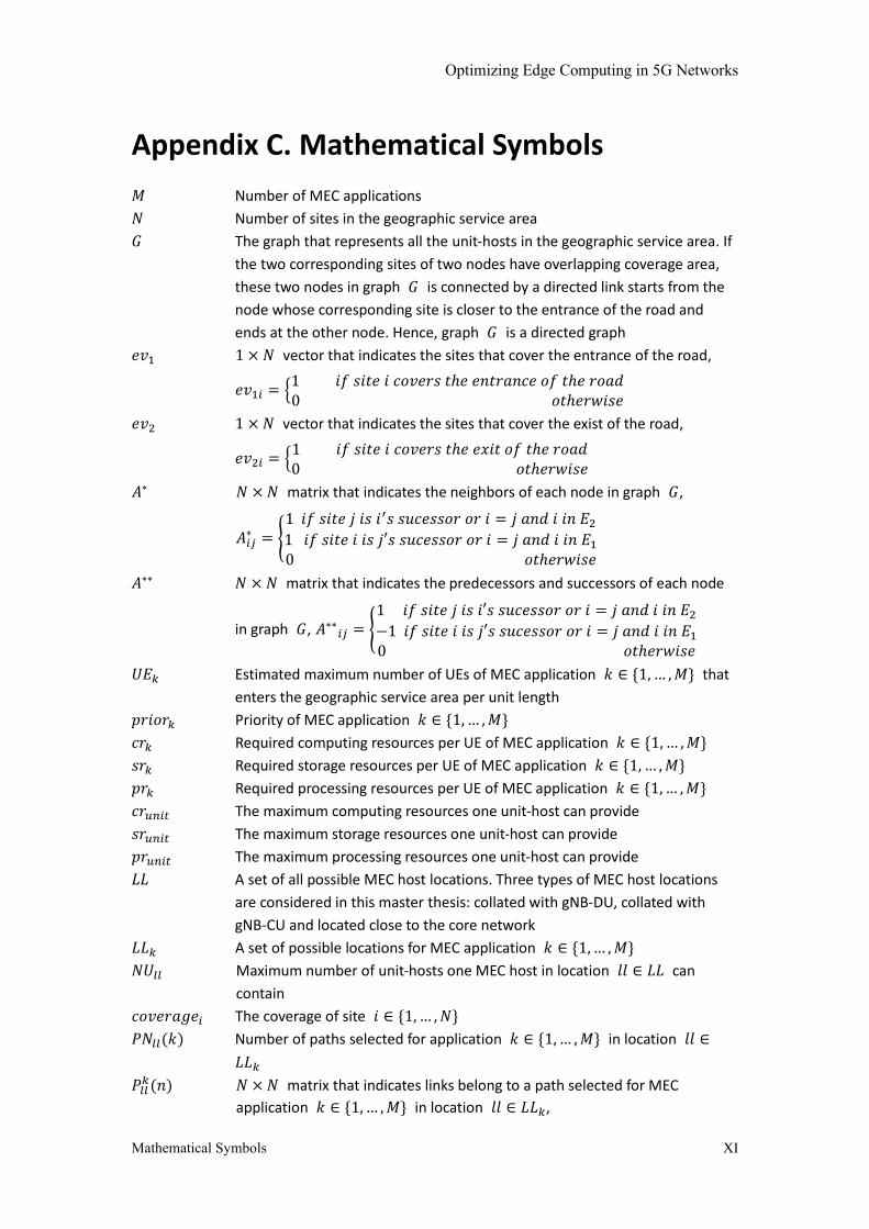
Optimizing Edge Computing in 5G Networks
Mathematical Symbols XI
Appendix C. Mathematical Symbols
𝑀 Number of MEC applications
𝑁 Number of sites in the geographic service area
𝐺 The graph that represents all the unit-hosts in the geographic service area. If
the two corresponding sites of two nodes have overlapping coverage area,
these two nodes in graph 𝐺 is connected by a directed link starts from the
node whose corresponding site is closer to the entrance of the road and
ends at the other node. Hence, graph 𝐺 is a directed graph
𝑒𝑣1 1 × 𝑁 vector that indicates the sites that cover the entrance of the road,
𝑒𝑣1𝑖 = {1 𝑖𝑓 𝑠𝑖𝑡𝑒 𝑖 𝑐𝑜𝑣𝑒𝑟𝑠 𝑡ℎ𝑒 𝑒𝑛𝑡𝑟𝑎𝑛𝑐𝑒 𝑜𝑓 𝑡ℎ𝑒 𝑟𝑜𝑎𝑑0 𝑜𝑡ℎ𝑒𝑟𝑤𝑖𝑠𝑒
𝑒𝑣2 1 × 𝑁 vector that indicates the sites that cover the exist of the road,
𝑒𝑣2𝑖 = {1 𝑖𝑓 𝑠𝑖𝑡𝑒 𝑖 𝑐𝑜𝑣𝑒𝑟𝑠 𝑡ℎ𝑒 𝑒𝑥𝑖𝑡 𝑜𝑓 𝑡ℎ𝑒 𝑟𝑜𝑎𝑑0 𝑜𝑡ℎ𝑒𝑟𝑤𝑖𝑠𝑒
𝐴∗ 𝑁 × 𝑁 matrix that indicates the neighbors of each node in graph 𝐺,
𝐴𝑖𝑗∗ = {
1 𝑖𝑓 𝑠𝑖𝑡𝑒 𝑗 𝑖𝑠 𝑖′𝑠 𝑠𝑢𝑐𝑒𝑠𝑠𝑜𝑟 𝑜𝑟 𝑖 = 𝑗 𝑎𝑛𝑑 𝑖 𝑖𝑛 𝐸2
1 𝑖𝑓 𝑠𝑖𝑡𝑒 𝑖 𝑖𝑠 𝑗′𝑠 𝑠𝑢𝑐𝑒𝑠𝑠𝑜𝑟 𝑜𝑟 𝑖 = 𝑗 𝑎𝑛𝑑 𝑖 𝑖𝑛 𝐸1
0 𝑜𝑡ℎ𝑒𝑟𝑤𝑖𝑠𝑒
𝐴∗∗ 𝑁 × 𝑁 matrix that indicates the predecessors and successors of each node
in graph 𝐺, 𝐴∗∗𝑖𝑗 = {
1 𝑖𝑓 𝑠𝑖𝑡𝑒 𝑗 𝑖𝑠 𝑖′𝑠 𝑠𝑢𝑐𝑒𝑠𝑠𝑜𝑟 𝑜𝑟 𝑖 = 𝑗 𝑎𝑛𝑑 𝑖 𝑖𝑛 𝐸2
−1 𝑖𝑓 𝑠𝑖𝑡𝑒 𝑖 𝑖𝑠 𝑗′𝑠 𝑠𝑢𝑐𝑒𝑠𝑠𝑜𝑟 𝑜𝑟 𝑖 = 𝑗 𝑎𝑛𝑑 𝑖 𝑖𝑛 𝐸1
0 𝑜𝑡ℎ𝑒𝑟𝑤𝑖𝑠𝑒
𝑈𝐸𝑘 Estimated maximum number of UEs of MEC application 𝑘 ∈ {1, … , 𝑀} that
enters the geographic service area per unit length
𝑝𝑟𝑖𝑜𝑟𝑘 Priority of MEC application 𝑘 ∈ {1, … , 𝑀}
𝑐𝑟𝑘 Required computing resources per UE of MEC application 𝑘 ∈ {1, … , 𝑀}
𝑠𝑟𝑘 Required storage resources per UE of MEC application 𝑘 ∈ {1, … , 𝑀}
𝑝𝑟𝑘 Required processing resources per UE of MEC application 𝑘 ∈ {1, … , 𝑀}
𝑐𝑟𝑢𝑛𝑖𝑡 The maximum computing resources one unit-host can provide
𝑠𝑟𝑢𝑛𝑖𝑡 The maximum storage resources one unit-host can provide
𝑝𝑟𝑢𝑛𝑖𝑡 The maximum processing resources one unit-host can provide
𝐿𝐿 A set of all possible MEC host locations. Three types of MEC host locations
are considered in this master thesis: collated with gNB-DU, collated with
gNB-CU and located close to the core network
𝐿𝐿𝑘 A set of possible locations for MEC application 𝑘 ∈ {1, … , 𝑀}
𝑁𝑈𝑙𝑙 Maximum number of unit-hosts one MEC host in location 𝑙𝑙 ∈ 𝐿𝐿 can
contain
𝑐𝑜𝑣𝑒𝑟𝑎𝑔𝑒𝑖 The coverage of site 𝑖 ∈ {1, … , 𝑁}
𝑃𝑁𝑙𝑙(𝑘) Number of paths selected for application 𝑘 ∈ {1, … , 𝑀} in location 𝑙𝑙 ∈
𝐿𝐿𝑘
𝑃𝑙𝑙𝑘(𝑛) 𝑁 × 𝑁 matrix that indicates links belong to a path selected for MEC
application 𝑘 ∈ {1, … , 𝑀} in location 𝑙𝑙 ∈ 𝐿𝐿𝑘,

Optimizing Edge Computing in 5G Networks
Mathematical Symbols XII
𝑃𝑙𝑙𝑘(𝑛)𝑖𝑗 = {
1 𝑖𝑓 𝑠𝑖𝑡𝑒 𝑖 𝑎𝑛𝑑 𝑗 𝑎𝑟𝑒 𝑐𝑜𝑛𝑛𝑒𝑐𝑡𝑒𝑑 𝑖𝑛 𝑝𝑎𝑡ℎ 𝑛 0 𝑜𝑡ℎ𝑒𝑟𝑤𝑖𝑠𝑒
(𝑛 = 1, … , 𝑃𝑁𝑙𝑙(𝑘))
𝐸𝑁𝑙𝑙𝑘(𝑛) 𝑁 × 𝑁 matrix that indicates the sites that cover either the entrance or the
exit of the road and belong to path 𝑛 ∈ {1, … , 𝑃𝑁𝑙𝑙(𝑘)} in location 𝑙𝑙 ∈
𝐿𝐿𝑘,
𝑃𝑙𝑙𝑘(𝑛)𝑖𝑗 = {
1 𝑖𝑓 𝑖 = 𝑗 𝑎𝑛𝑑 𝑠𝑖𝑡𝑒 𝑖 𝑖𝑛 𝑝𝑎𝑡ℎ 𝑛 𝑎𝑛𝑑 𝑖 𝑖𝑛 𝐸1 𝑜𝑟 𝐸2
0 𝑜𝑡ℎ𝑒𝑟𝑤𝑖𝑠𝑒
𝑈𝐸𝑃𝑙𝑙𝑘(𝑛) Estimated number of UEs per unit length of MEC application 𝑘 ∈ {1, … , 𝑀}
of path 𝑛 ∈ {1, … , 𝑃𝑁𝑙𝑙(𝑘)} in location 𝑙𝑙 ∈ 𝐿𝐿𝑘
𝐻𝑁𝑙𝑙 Number of MEC hosts in location 𝑙𝑙 ∈ 𝐿𝐿
𝐻𝑙𝑙(𝑚) 𝑁 × 𝑁 matrix that indicates the links inside MEC host 𝑚,
𝐻𝑙(𝑚)𝑖𝑗 = {1 𝑖𝑓 𝑠𝑖𝑡𝑒 𝑖 𝑎𝑛𝑑 𝑗 𝑎𝑟𝑒 𝑐𝑜𝑛𝑛𝑒𝑐𝑡𝑒𝑑 𝑎𝑛𝑑 𝑏𝑜𝑡ℎ 𝑖𝑛 ℎ𝑜𝑠𝑡 𝑚1 𝑖𝑓 𝑖 = 𝑗 𝑎𝑛𝑑 𝑠𝑖𝑡𝑒 𝑖 𝑖𝑛 ℎ𝑜𝑠𝑡 𝑚0 𝑜𝑡ℎ𝑒𝑟𝑤𝑖𝑠𝑒
(𝑚 = 1, … , 𝐻𝑁𝑙𝑙 , 𝑙𝑙 ∈ 𝐿𝐿)
𝑃𝐿(𝑘) The total length of paths selected for MEC application 𝑘 ∈ {1, … , 𝑀}
𝑅𝐸(𝑘) The total number of relocations UEs of MEC application 𝑘 ∈ {1, … , 𝑀}
experience
𝐷𝐿(𝑘) The number of disappeared links which belong to the paths selected for MEC
application 𝑘 ∈ {1, … , 𝑀} in graph 𝐺 by merging nodes in the way that
matrices {𝐻𝑙𝑙(𝑚)}(∀ 𝑙𝑙 ∈ 𝐿𝐿) imply
𝐸𝑅(𝑘) The total number of eliminated relocations of MEC application 𝑘 ∈
{1, … , 𝑀} by merging nodes in graph 𝐺 in the way that matrices
{𝐻𝑙𝑙(𝑚)}(∀ 𝑙𝑙 ∈ 𝐿𝐿) imply
𝐸𝑅𝑊(𝑘) The total weighted number of eliminated relocations of MEC application 𝑘 ∈
{1, … , 𝑀} by merging nodes in graph 𝐺 in the way that matrices
{𝐻𝑙𝑙(𝑚)}(∀ 𝑙𝑙 ∈ 𝐿𝐿) imply
𝑅𝐸𝑊(𝑘) The total weighted number of relocations UEs of MEC application 𝑘 ∈
{1, … , 𝑀} experience before integrating unit-hosts into MEC hosts
𝑅𝑊 The total weighted number of relocations of all MEC applications after
integrating unit-hosts into MEC hosts
𝐿𝑊𝑙𝑙 A set of link weights of all links which both end nodes are in location 𝑙𝑙 ∈ 𝐿𝐿
𝐸1 A set of unit-hosts which corresponding sites cover the entrance of the road
in the geographic service area
𝐸2 A set of unit-hosts which corresponding sites cover the exit of the road in the
geographic service area
𝑅𝑙𝑙 A set of currently available resources in all unit-hosts in location 𝑙𝑙 ∈ 𝐿𝐿
𝑟𝑒𝑠𝑜𝑢𝑟𝑐𝑒𝑠𝑘 Required amount of resources per UE of MEC application 𝑘 ∈ {1, … , 𝑀}
𝑃𝑎𝑡ℎ𝑠𝑙𝑙(𝑘) A set that saves all paths in location 𝑙𝑙 ∈ 𝐿𝐿𝑘 that are selected to reserve
resources for MEC application 𝑘 ∈ {1, … , 𝑀} as well as the number of UEs
each path serves
𝐻𝑙𝑙 𝐻𝑙𝑙 = {ℎ1, ℎ2, … , ℎ𝑚}, where ℎ𝑖 is a set of all unit-hosts that belong to an
already existed MEC host 𝑖 in location 𝑙𝑙 ∈ 𝐿𝐿, 𝑚 is the current number of
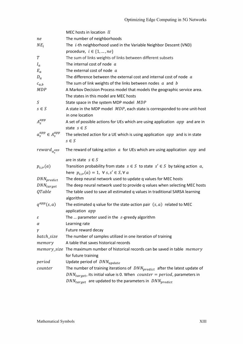
Optimizing Edge Computing in 5G Networks
Mathematical Symbols XIII
MEC hosts in location 𝑙𝑙
𝑛𝑒 The number of neighborhoods
𝑁𝐸𝑖 The 𝑖-th neighborhood used in the Variable Neighbor Descent (VND)
procedure, 𝑖 ∈ {1, … , 𝑛𝑒}
𝑇 The sum of links weights of links between different subsets
𝐼𝑎 The internal cost of node 𝑎
𝐸𝑎 The external cost of node 𝑎
𝐷𝑎 The difference between the external cost and internal cost of node 𝑎
𝑐𝑎,𝑏 The sum of link weights of the links between nodes 𝑎 and 𝑏
𝑀𝐷𝑃 A Markov Decision Process model that models the geographic service area.
The states in this model are MEC hosts
𝑆 State space in the system MDP model 𝑀𝐷𝑃
𝑠 ∈ 𝑆 A state in the MDP model 𝑀𝐷𝑃, each state is corresponded to one unit-host
in one location
𝐴𝑠𝑎𝑝𝑝
A set of possible actions for UEs which are using application 𝑎𝑝𝑝 and are in
state 𝑠 ∈ 𝑆
𝑎𝑠𝑎𝑝𝑝
∈ 𝐴𝑠𝑎𝑝𝑝
The selected action for a UE which is using application 𝑎𝑝𝑝 and is in state
𝑠 ∈ 𝑆
𝑟𝑒𝑤𝑎𝑟𝑑𝑎𝑠𝑎𝑝𝑝 The reward of taking action 𝑎 for UEs which are using application 𝑎𝑝𝑝 and
are in state 𝑠 ∈ 𝑆
𝑝𝑠,𝑠′(𝑎) Transition probability from state 𝑠 ∈ 𝑆 to state 𝑠′ ∈ 𝑆 by taking action 𝑎,
here 𝑝𝑠,𝑠′(𝑎) = 1, ∀ 𝑠, 𝑠′ ∈ 𝑆, ∀ 𝑎
𝐷𝑁𝑁𝑝𝑟𝑒𝑑𝑖𝑐𝑡 The deep neural network used to update q values for MEC hosts
𝐷𝑁𝑁𝑡𝑎𝑟𝑔𝑒𝑡 The deep neural network used to provide q values when selecting MEC hosts
𝑄𝑇𝑎𝑏𝑙𝑒 The table used to save all estimated q values in traditional SARSA learning
algorithm
𝑞𝑎𝑝𝑝(𝑠, 𝑎) The estimated q value for the state-action pair (𝑠, 𝑎) related to MEC
application 𝑎𝑝𝑝
𝜀 The … parameter used in the 𝜀-greedy algorithm
𝛼 Learning rate
𝛾 Future reward decay
𝑏𝑎𝑡𝑐ℎ_𝑠𝑖𝑧𝑒 The number of samples utilized in one iteration of training
𝑚𝑒𝑚𝑜𝑟𝑦 A table that saves historical records
𝑚𝑒𝑚𝑜𝑟𝑦_𝑠𝑖𝑧𝑒 The maximum number of historical records can be saved in table 𝑚𝑒𝑚𝑜𝑟𝑦
for future training
𝑝𝑒𝑟𝑖𝑜𝑑 Update period of 𝐷𝑁𝑁𝑢𝑝𝑑𝑎𝑡𝑒
𝑐𝑜𝑢𝑛𝑡𝑒𝑟 The number of training iterations of 𝐷𝑁𝑁𝑝𝑟𝑒𝑑𝑖𝑐𝑡 after the latest update of
𝐷𝑁𝑁𝑡𝑎𝑟𝑔𝑒𝑡, its initial value is 0. When 𝑐𝑜𝑢𝑛𝑡𝑒𝑟 = 𝑝𝑒𝑟𝑖𝑜𝑑, parameters in
𝐷𝑁𝑁𝑡𝑎𝑟𝑔𝑒𝑡 are updated to the parameters in 𝐷𝑁𝑁𝑝𝑟𝑒𝑑𝑖𝑐𝑡

Optimizing Edge Computing in 5G Networks
Expert Interviews XV
Appendix D. Expert Interviews
Interview Questions and Answers
1. How many MEC hosts do you estimate (order of magnitude) in the Netherlands in the
initial stage of Multi-access Edge Computing deployment and 5 years later?
At the very early stage, the number of MEC hosts will be limited. But when the O&M
cost can be reduced significantly and the number of end-users of MEC services are
substantial enough, the number of MEC hosts will increase. However, the number of
MEC hosts in 5 years’ time is currently hard to predict. (Question answered in interviews
1, 2 and 3)
2. At which levels in the telecom hierarchy of the network of a Dutch Telco and at which
locations of a telecom network would you position MEC hosts initially and after 5 years
of deployment?
KPN will position MEC hosts at its Metro Cores and superior Cores, as well as locations
near to the end-users of MEC services. Because for KPN, optimizing fiber routes can bring
more benefits than locating the MEC hosts closer to the end-users. For use cases like
V2X offloading and on-premise industrial deployments, however, MEC hosts need to be
placed closer to the vehicles; for example, along the roadside or physically close to the
factory etc. (Question answered in interviews 2 and 3)
3. How do you estimate the normal coverage of a MEC host (with/without virtualization) in
the initial stage and 5 years later?
Right now, KPN locates MEC hosts at its 4 superior Core location within the Netherlands.
Later on MEC hosts may be moved to the 164 Metro Core locations to further reduce
the latency. However, as the cost will increase by doing so, therefore further research is
required. When a MEC host is co-located with a core/metro core, it will provide MEC
services to the UEs that are served by the corresponding core/metro core serving area.
In the future, it is hard to predict the serving coverage of a MEC host, which may depend
on the usage, development and benefits of MEC as well as the maintenance and other
costs of running a MEC host close to the network edge. (Question answered in interviews
2 and 3)
4. Would you think it is necessary for MEC hosts to always connect to (a) (virtualized) UPF(s)?
At least foreseen up to now, it is necessary. A MEC host needs to receive the user data it
requires while still under the control of the core network, and UPF is the element that
can steer the required data towards a MEC host and get controlled by the core network
via control plane signaling. (Question answered in interviews 1, 2 and 3)
5. How do you estimate the complexity and costs (both time and resource/money-wise) of
installing MEC applications and instantiating MEC application instances in MEC hosts?
Instantiating a MEC application instance on demand can be done within several
milliseconds. However, installing a MEC application in a MEC host can take several
seconds. Besides, the transfer of user context data between the old and new MEC hosts
for a stateful/dedicated MEC application is the major source of delay during a relocation.
(Question answered in interview 2)
Optimizing Edge Computing in 5G Networks
Expert Interviews XVI
6. Do you think it is possible that one UPF can be connected to CU-UPs from different CUs?
Do you think it is possible that one CU-UP can connect to multiple UPFs?
The answer to both questions is yes. The number of CUs in a network is much larger than
the number of UPFs in a network, so a UPF has to be able to connect to multiple CUs. A
UE may have multiple requests to access to different data networks via different UPFs,
however, user data may go through the same CU-UP, so it is possible for a CU-UP to
connect to several UPFs. (Question answered in interview 3)
7. Do you agree that service latency between a UE and a MEC host is largely dependent on
the locations (physical and/or logical) of MEC hosts in the network?
Yes, service latency largely depends on both logical and physical locations of MEC hosts.
The logical location of a MEC host determines how many functional entities between
the UE and the MEC host are involved in delivering MEC services. Since the optical fiber
related transmission time is negligible (especially in small-sized countries such as The
Netherlands), the processing and queueing time at each functional entity in between
mainly determines the service latency. Besides, the physical location of a MEC host also
matters because the transmission nodes in between need time to do coding and
decoding as well as transformation of the received data. The closer the physical location
of a MEC host is to the UE, the fewer transmission nodes in between and thus the shorter
service latency between the UE and the MEC host. (Question answered in interview 1)
Interview 1
Expert: Jan Backman
Position: Expert Packet Core Mobility Architecture
Enterprise: Ericsson
Date: Monday, September 21st, 2020
Time slot: 15:00 – 16:00
Form: Microsoft Teams
Summary:
1. Transmission time on optical fibers is negligible. Sending a packet between the southern
part of the Netherlands and the northern part of the Netherlands on optical fibers only
takes 1.5 milliseconds back-and-forth. Likewise, sending a packet between the northern
part of Sweden and the southern part of Sweden on optical fibers only takes around 2
milliseconds back-and-forth.
2. Transmission time via a 5G New Radio (NR) air interface between a UE and a gNB is
around 8 milliseconds back-and-forth. Compared to optical fiber, this delay is much
higher, but it is inevitable.
3. Since the transmission time on optical fibers is negligible, one of the major sources of
latencies is the processing time and queueing time of functional entities between the
UE and the MEC host.
4. Service latency may not be the main driver of MEC deployment, to reduce half of the
latency, only 4 times as many MEC hosts are needed. Instead, the population density/UE
density of an area may require more MEC hosts in order to fulfill the requirements of all
UEs in this area. In large cities, there will be more demands on MEC, hence more MEC
hosts needed and maybe some extra MEC hosts used for resiliency. In rural areas,

Optimizing Edge Computing in 5G Networks
Expert Interviews XVII
although the number of UEs is limited, MEC hosts need to be deployed in these locations
as well to serve the UEs there, which is costly but there is no better approach.
5. For telecom operators, investments and benefits are one of their main concerns. At the
initial stage, telecom operators may want to reuse their existing data centers.
6. With network function virtualization, functional entities in a 5G network can be placed
anywhere where hardware is available. Theoretically, the service latency can be reduced
significantly by placing the MEC hosts very close to the UEs. However, from the
operators’ point of view, although the deployment of MEC hosts is easier and cheaper
with the help of virtualization, the operational and maintenance (O&M) costs of
software is still high. Therefore, telecom operators do not want too many MEC hosts at
the initial stage. As the technology develops, the O&M costs may be reduced in the near
future and as more applications/devices require MEC services, by then telecom
operators will consider to build more MEC hosts.
7. In Atlantic City in the U.S., in order to save costs, there are only seven integrated base
stations in place, located in a circle around the city. Operators use Virtual RAN (V-RAN)
technology, a large number of small sites that cover the entire city will send user data
towards these seven base stations for aggregated processing, load-balancing
management, etc. In this way, the operating cost is significantly decreased.
8. To sum up, at the initial stage of MEC, the number of MEC hosts will be limited, mainly
due to the financial consequences for telecom operators. However, in the future, with
MEC and other related technology developing, MEC can be needed more widely and the
number of MEC hosts will increase at the same time.
Interview 2
Expert: Ir. Geerd Kakes
Position: Advisor
Enterprise: KPN
Date: Friday, October 2nd, 2020 & Monday, October 5th, 2020
Time slot: 13:00 – 14:00 & 11:30 – 12:30
Form: Microsoft Teams
Summary:
1. Distances in the Netherlands are small between radio sites and core location. For
instance, when moving a compute node from a Metro Core node (KPN has around 160
MC locations in NL) to the superior level of 4 core locations the latency gains around 1
to 2 milliseconds.
2. KPN will gain more performance from optimizing fiber routes than by bringing the
computing resources closer to the user. Some routes with an actual distance of a few
kilometers have a fiber length of more than 40 kilometers. This is because service
latency was not a main concern in the past and KPN implemented fiber rings which
result in a shorter path and a longer path between a UE and computing resources. After
the fiber routes are optimized, it can be foreseen that in some local areas the service
latency still cannot be satisfied, therefore more MEC hosts closer to the edge will be
needed.
3. Four use cases of edge computing are listed below:
Optimizing Edge Computing in 5G Networks
Expert Interviews XVIII
a) Increasing the network performance by bringing content closer to the end-user (e.g.
with Netflix content servers) or by processing data closer to the end-user (e.g. video
processing of surveillance cameras)
b) Decreasing latency for non-mobile users (e.g. gaming), currently the domain of fixed
access
c) Decreasing latency and resilience for V2X use cases (relevant after 2025)
d) Enabling factory automation with on premise 5G infrastructure
4. Edge computing locations at the initial stage will be limited to the following situations:
a) KPN’s 4 superior core locations for mobility use cases
b) Metro Core location to increase network performance
c) Customer locations to enable factory or logistic use cases
5. On premise deployment of MEC can guarantee a real constant service latency to the
customers and end-users, and the MEC hosts will be located closer to the edge than at
the metro core locations. Besides, on premise deployment allows the customers to
control their own data security.
6. For V2X scenario, the communications between self-driving vehicles can be done by
short range communications like Destination-to-Destination (D2D) communication. In
this approach, no MEC hosts are needed. A vehicle can communicate with its peers
nearby by broadcasting its location and direction information. However, this type of
communication cannot be verified. A vehicle which receives the broadcasted
information will not send a response to the vehicle that broadcasts the information,
therefore the vehicle which broadcasts the information will never know whether the
messages are correctly received by all the vehicles within its vicinity or not. To enhance
the success rate of message transfers between vehicles, each vehicle will keep
broadcasting the same information (maybe with few updates) repeatedly (e.g. 10 times
per second).
7. Some information which has a large data volume and is not updated frequently can be
transferred via long range communication methods, for example via TCP. TCP
guarantees that the data will be received correctly by the receivers and will send a
verification to the sender. Although this approach might take longer time, it is suitable
for information like map information of the road which contains the overview of the
entire road. This type of information will not change frequently and contains a large
amount of data, so it is not necessary to broadcast it periodically and create a large
volume of redundancy. Therefore, long range communication is the better choice here.
8. For transferring critical information, D2D communication requires the vehicle itself to
sign the message and verify the source of the received message, which involves
decoding and analyzing procedure that is time-consuming. Some first measurements
using a generic processor show an extra latency of around 13ms. In long range
communication, however, the network itself will do the verification for the vehicles,
consider the much larger amount of computing and processing resources in the network
than in a vehicle. Thus, long range communication can be faster than short range
communication under this situation.
9. There are debates on where the received information from vehicles nearby should be
computed and processed. Some hold the opinion that considering the low cost of

Optimizing Edge Computing in 5G Networks
Expert Interviews XIX
hardware, it is possible to do the computing and processing inside a vehicle, while others
think this approach is not reliable. With the help of MEC, the computation of a vehicle
can be offloaded to the MEC host physically close to the vehicle, which can speed up
computation and possibly enhance reliability. In this case, the MEC hosts should be
deployed very close to the vehicles and the MEC service continuity should be
guaranteed.
10. If the trajectory of a vehicle is fully predictable, the MEC application instance in the
target MEC host can be instantiated in advance, so the vehicle can connect to the new
MEC host before it loses the connection towards the current MEC host. However, in real
situations, accurate predications cannot be guaranteed sometimes, if a vehicle connects
to a new MEC host before the required MEC application instance in the new MEC host
is ready, it can still connect to the previous MEC host via the new one. In this case, the
service latency mainly comes from the latency between two MEC hosts instead of the
latency between the UE and the new MEC host.
11. Launching a MEC application (instantiating a MEC application instance) on demand can
be done easily and quickly with current technology within several milliseconds. However,
installing a MEC application in a MEC host can take several seconds. Although the MEC
application image can be easily pre-loaded in a MEC host with almost no cost at all,
loading a container is rather time-consuming.
Interview 3
Expert: Dr. ing. Frank Mertz
Position: Designer
Enterprise: KPN
Date: Monday, October 5th, 2020
Time slot: 13:00 – 13:30
Form: Microsoft Teams
Summary:
1. The current possible locations for MEC at KPN is at the four superior core locations in
the Netherlands. Later, MEC hosts may be moved to the Metro Core locations that KPN
has in place in the Netherlands, 161 in total, if the benefits have been proved. Besides,
the on-premise deployments will put the MEC host physically close to the place where
MEC services are required by the customer, for example, a factory. In the future, it is
hard to say where possible locations of MEC hosts can be, but it is always the case that
telecom operators want to maximize their benefits and currently, running and
maintaining a MEC host is costly, hence the number of MEC hosts needs to be limited,
unless the maintenance cost decreases and the profits provided by MEC increases in the
future.
2. Up to now, a MEC host is always collocated with at least one (local) UPF, because the
user data required by a MEC hosts needs to be steered by UPFs. Besides, traffic steering
should always under the control of the core network, using UPF can make sure MEC
applications do not fiddle with the traffic rules, because traffic rules followed by a UPF
is controlled by PCF via SMF instead of the MEC application itself.

Optimizing Edge Computing in 5G Networks
Expert Interviews XX
3. A UPF can connect to multiple CU-UPs that are controlled by different CU-CPs at the
same time. In this sense, a 5G network is similar to a 4G network. In the Netherlands,
KPN has only 4 P-Gws but around 5000 base stations in the current 4G network. This
means that one P-Gw should be able to serve multiple base stations. Even though in 4G
technology, an eNodeB is not split into multiple DUs, one CU-CP and multiple CU-UPs,
the basic concept is the same; one P-Gw can serve multiple base stations which means
that it can be connected to multiple user planes that are controlled by multiple control
planes in different base stations.
4. A CU-UP can be connected to multiple UPFs at the same time. Nowadays, one single UE
may have multiple requirements to different data networks. Take mobile phone as an
example, a user may require for Internet connection and IMS connection at the same
time. To connect to multiple data networks, the UE may be connected to multiple UPFs,
but on the radio side of the network, all the user data may be transferred via the same
CU-UP, therefore, one single CU-UP should be able but not necessarily to connect to
multiple UPFs. Theoretically, it is possible to build one CU-UP for each UPF, but consider
the high cost of implementing and maintaining one functional element even with the
help of network virtualization, connecting one CU-UP to multiple CU-UPs seems to be
the better option at present.

Optimizing Edge Computing in 5G Networks
Location Service XXI
Appendix E. Location Service
Location Service provides services including UE Location Lookup, UE Information Lookup, UE
Location Subscribe, UE Information Subscribe, Subscribe Cancellation, Radio Node Location
Lookup, UE Tracking Subscribe, UE Distance Lookup, UE Distance Subscribe and UE Area
Subscribe. Only a few relevant services are further introduced.
UE Location Lookup
The UE Location Lookup can provide the current location information of a single UE or a group
of UEs. The Location Service will report the lookup result once on each request. Figure E.1
illustrates the procedure of UE Location Lookup.
Figure E.1: Flow of UE Location Lookup [32].
1. The MEC application/MEC platform which wants to look up one or more UE locations
sends a request with the identifier for each UE (e.g. UE IP address). The request includes
one or more query parameters to specify the interested UE(s).
2. The Location Service returns a response with the location information of the requested
UE(s).
Radio Node Location Lookup
The Radio Node Location Lookup is to retrieve the radio nodes that are currently associated
with a MEC host. Figure E.2 illustrates the procedure of Radio Node Location Lookup.
Figure E.2: Flow of Radio Node Location Lookup [32].
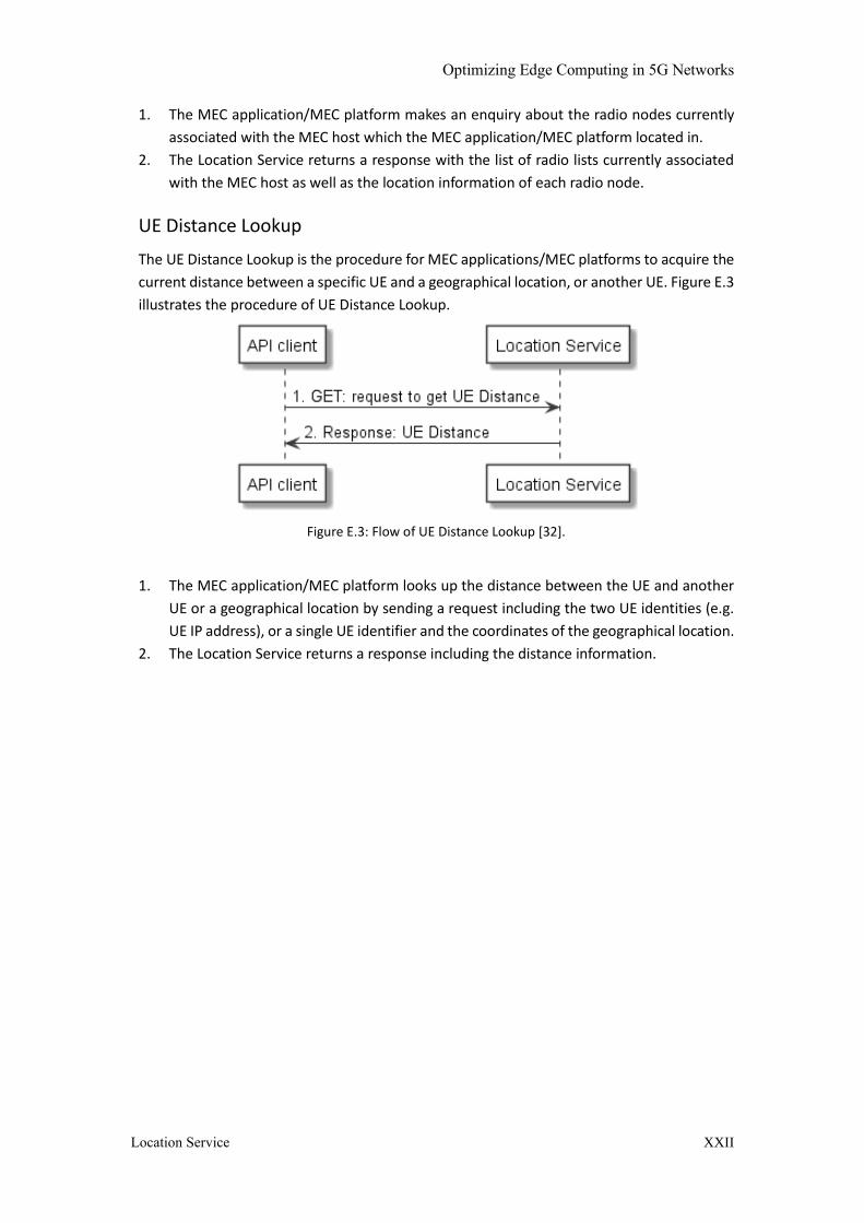
Optimizing Edge Computing in 5G Networks
Location Service XXII
1. The MEC application/MEC platform makes an enquiry about the radio nodes currently
associated with the MEC host which the MEC application/MEC platform located in.
2. The Location Service returns a response with the list of radio lists currently associated
with the MEC host as well as the location information of each radio node.
UE Distance Lookup
The UE Distance Lookup is the procedure for MEC applications/MEC platforms to acquire the
current distance between a specific UE and a geographical location, or another UE. Figure E.3
illustrates the procedure of UE Distance Lookup.
Figure E.3: Flow of UE Distance Lookup [32].
1. The MEC application/MEC platform looks up the distance between the UE and another
UE or a geographical location by sending a request including the two UE identities (e.g.
UE IP address), or a single UE identifier and the coordinates of the geographical location.
2. The Location Service returns a response including the distance information.
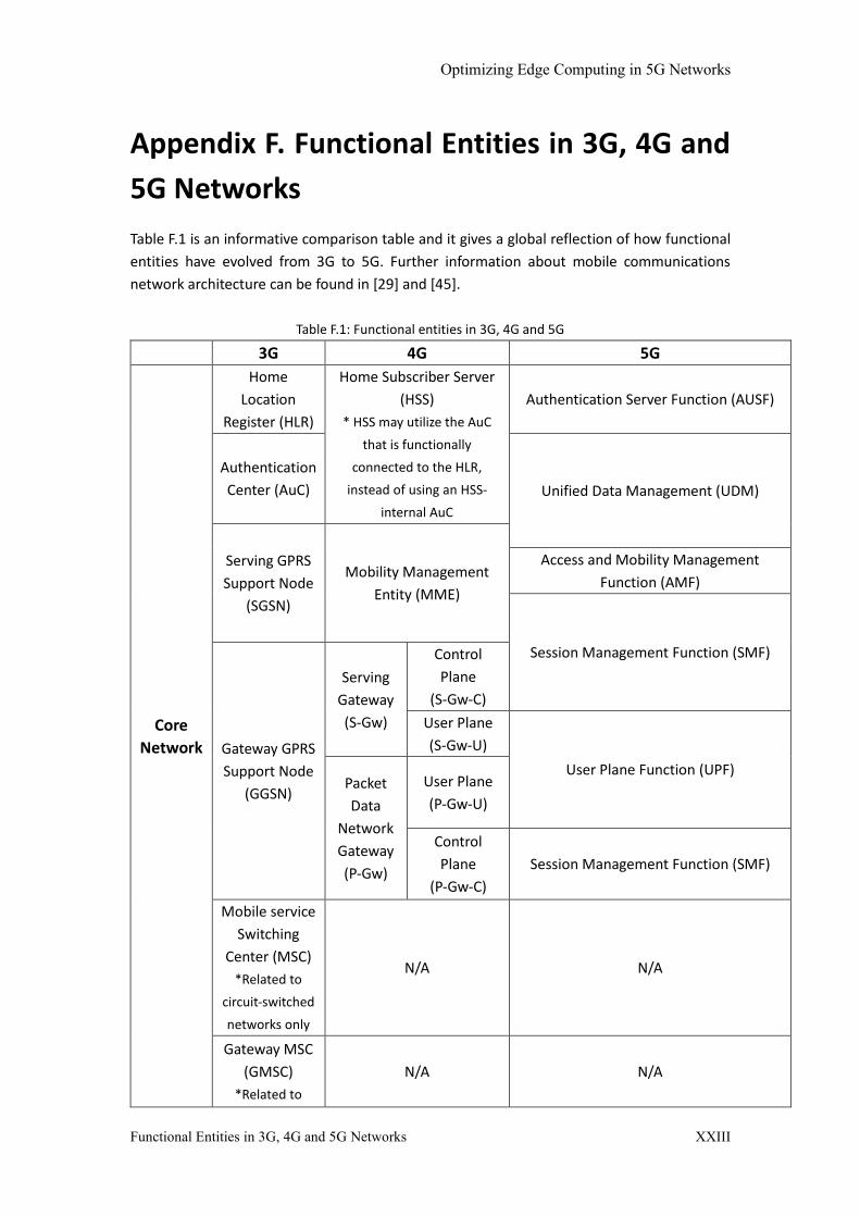
Optimizing Edge Computing in 5G Networks
Functional Entities in 3G, 4G and 5G Networks XXIII
Appendix F. Functional Entities in 3G, 4G and
5G Networks
Table F.1 is an informative comparison table and it gives a global reflection of how functional
entities have evolved from 3G to 5G. Further information about mobile communications
network architecture can be found in [29] and [45].
Table F.1: Functional entities in 3G, 4G and 5G
3G 4G 5G
Core
Network
Home
Location
Register (HLR)
Home Subscriber Server
(HSS)
* HSS may utilize the AuC
that is functionally
connected to the HLR,
instead of using an HSS-
internal AuC
Authentication Server Function (AUSF)
Authentication
Center (AuC) Unified Data Management (UDM)
Serving GPRS
Support Node
(SGSN)
Mobility Management
Entity (MME)
Access and Mobility Management
Function (AMF)
Session Management Function (SMF)
Gateway GPRS
Support Node
(GGSN)
Serving
Gateway
(S-Gw)
Control
Plane
(S-Gw-C)
User Plane
(S-Gw-U)
User Plane Function (UPF) Packet
Data
Network
Gateway
(P-Gw)
User Plane
(P-Gw-U)
Control
Plane
(P-Gw-C)
Session Management Function (SMF)
Mobile service
Switching
Center (MSC)
*Related to
circuit-switched
networks only
N/A N/A
Gateway MSC
(GMSC)
*Related to
N/A N/A
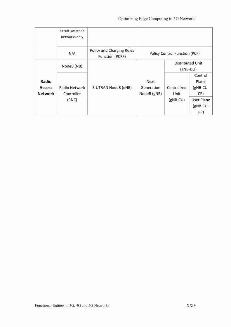
Optimizing Edge Computing in 5G Networks
Functional Entities in 3G, 4G and 5G Networks XXIV
circuit-switched
networks only
N/A Policy and Charging Rules
Function (PCRF) Policy Control Function (PCF)
Radio
Access
Network
NodeB (NB)
E-UTRAN NodeB (eNB)
Next
Generation
NodeB (gNB)
Distributed Unit
(gNB-DU)
Radio Network
Controller
(RNC)
Centralized
Unit
(gNB-CU)
Control
Plane
(gNB-CU-
CP)
User Plane
(gNB-CU-
UP)
Related Documents