Optimizing Cleaning Schedules of Heat Exchanger Networksieomsociety.org/ieomdetroit/pdfs/162.pdf · Consequently, Heat Exchanger Cleanings amount to a massive operating expenditure

Proceedings of the 2016 International Conference on Industrial Engineering and Operations Management

Detroit, Michigan, USA, September 23-25, 2016

© IEOM Society International

Optimizing Cleaning Schedules of Heat Exchanger Networks

Mohamed Elsholkami, Muhummad Bajwa, Matthew Aydemir, Terell Brown, Dinesha

Ganesarajan, Ali Elkamel, and Chandra Mouli Madhuranthakam

Department of Chemical Engineering

University of Waterloo

Waterloo, ON N2L 3G1, Canada

[email protected], [email protected], [email protected]

Abstract

Fouling in Heat Exchangers is a serious operating problem in many industries. It drastically reduces heat

transfer effectiveness and consequently, the rate of heat transfer. Fouling also causes difficulty in

maintaining key temperatures within their operating envelopes, as well as it imposes severe hydraulic

limitations to passing fluids through the heat exchanger. To combat fouling, heat exchangers must be

periodically removed from service and cleaned. This is a costly expense, but not taking the heat exchanger

out of service proves costly to downstream operations. More often than not, the undesired outlet temperature

from the heat exchanger would demand a higher energy consumption further downstream to mitigate the

problem. This trade-off implies an optimal time to clean the heat exchanger. In this study an approach was

developed where operating process data can be used to predict the rate of fouling and be used in an

optimization model to generate the optimal cleaning schedule. The project served to illustrate this idea by

employing it in a rapidly fouling Heat Exchanger Network (HEN). A HEN in a SAGD Facility is considered

and potential savings of $30,000 per month are illustrated through the use of this approach. Management

of fouling is a multi-billion dollar global problem and our solution has been proven to eliminate substantial

amounts of unnecessary cleaning expenditures.

Keywords

Optimization, MINLP, Heat exchanger networks, Scheduling

1. Introduction and background

Heat Exchanger fouling is one of the most common and troublesome issues in process industries. Fouling can lead

to losses in operational efficiency and ultimately increase a heat exchanger’s maintenance/operational cost. The total

fouling related costs for major industrialised nations is estimated to exceed US$4.4 Billion annually (Ibrahim, 2012),

or roughly 1% of their GDP. Evidently, fouling related costs are a major pain point for companies in a various range

of industries. An exchanger will typically foul up as foulants in process streams begin in to agglomerate on the surface

of tubes. There are two ways of understanding this phenomena: 1) a build-up of foulants adds an extra layer of thermal

resistance; thereby reducing the Overall Heat Transfer Coefficient (OHTC). This reduces total heat transfer

effectiveness between process streams, and 2) a build-up of foulants also increases the frictional pressure drop across

the heat-exchanger, thereby limiting the amount of flow that can be passed through the exchanger.

To counter-act fouling, heat exchangers are commonly taken out of service for cleaning. The typical modes of

cleaning are as follows: 1) chemical Cleaning – Exchangers are taken out of service and a chemical solution is injected

to extract out the foulant materials. The cost of these is anywhere from $ 10’000 - $ 50’000 (Ibrahim, 2012). A major

contributor to high Operating Expenditures at any plant. This takes about a day and typically engineering service

companies provide this service. Some companies (for e.g. MEG Energy in their Oil Sands facility) tend to perform

bake-outs. This involves shutting down the supply of the cold stream and heating up the exchanger with the hot stream.

The increase in temperature tends to eliminate deposited foulants. This ensures that the Heat Exchanger never goes

out of service, and 2) mechanical Cleaning – these methods include the injection of molded plastic cleaners (PIGS)

that go inside the tube and remove fouling through mechanical means. These methods are commonly employed where

Chemical Cleaning methods do not adequately eliminate fouling.

319

mailto:[email protected]






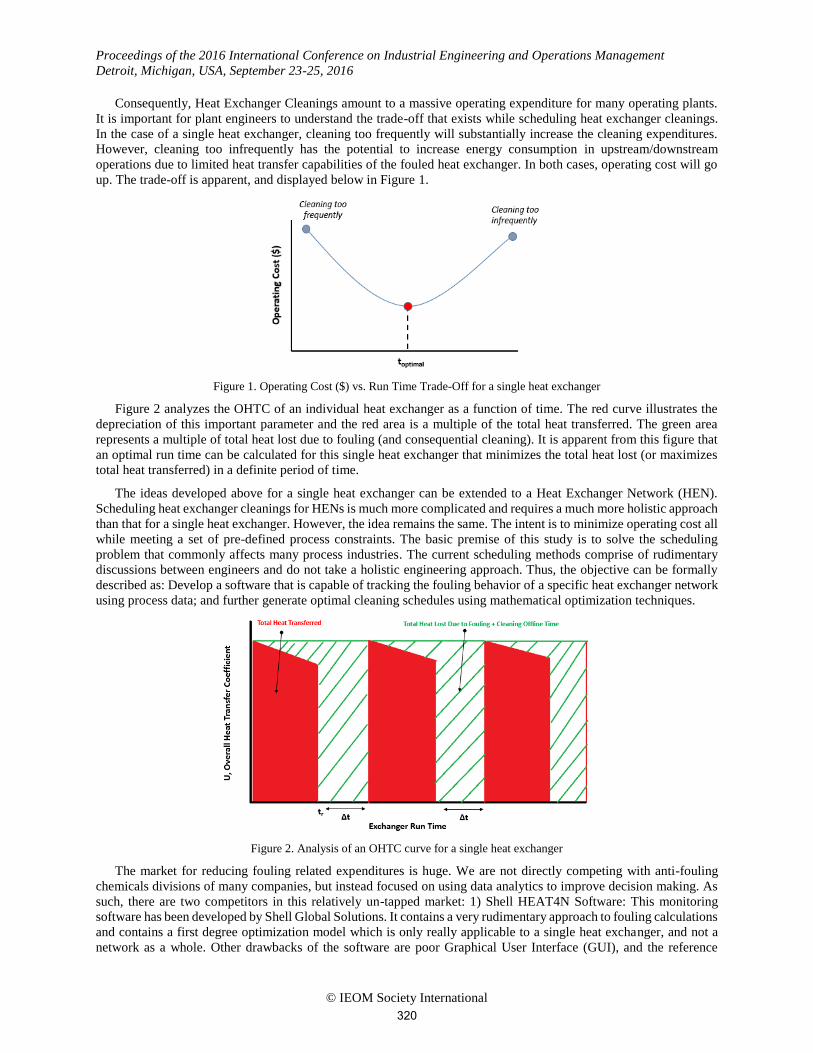
Consequently, Heat Exchanger Cleanings amount to a massive operating expenditure for many operating plants.

It is important for plant engineers to understand the trade-off that exists while scheduling heat exchanger cleanings.

In the case of a single heat exchanger, cleaning too frequently will substantially increase the cleaning expenditures.

However, cleaning too infrequently has the potential to increase energy consumption in upstream/downstream

operations due to limited heat transfer capabilities of the fouled heat exchanger. In both cases, operating cost will go

up. The trade-off is apparent, and displayed below in Figure 1.

Figure 1. Operating Cost ($) vs. Run Time Trade-Off for a single heat exchanger

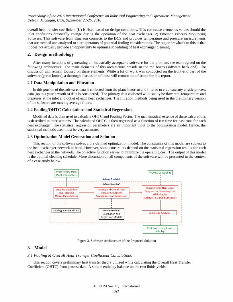
Figure 2 analyzes the OHTC of an individual heat exchanger as a function of time. The red curve illustrates the

depreciation of this important parameter and the red area is a multiple of the total heat transferred. The green area

represents a multiple of total heat lost due to fouling (and consequential cleaning). It is apparent from this figure that

an optimal run time can be calculated for this single heat exchanger that minimizes the total heat lost (or maximizes

total heat transferred) in a definite period of time.

The ideas developed above for a single heat exchanger can be extended to a Heat Exchanger Network (HEN).

Scheduling heat exchanger cleanings for HENs is much more complicated and requires a much more holistic approach

than that for a single heat exchanger. However, the idea remains the same. The intent is to minimize operating cost all

while meeting a set of pre-defined process constraints. The basic premise of this study is to solve the scheduling

problem that commonly affects many process industries. The current scheduling methods comprise of rudimentary

discussions between engineers and do not take a holistic engineering approach. Thus, the objective can be formally

described as: Develop a software that is capable of tracking the fouling behavior of a specific heat exchanger network

using process data; and further generate optimal cleaning schedules using mathematical optimization techniques.

Figure 2. Analysis of an OHTC curve for a single heat exchanger

The market for reducing fouling related expenditures is huge. We are not directly competing with anti-fouling

chemicals divisions of many companies, but instead focused on using data analytics to improve decision making. As

such, there are two competitors in this relatively un-tapped market: 1) Shell HEAT4N Software: This monitoring

software has been developed by Shell Global Solutions. It contains a very rudimentary approach to fouling calculations

and contains a first degree optimization model which is only really applicable to a single heat exchanger, and not a

network as a whole. Other drawbacks of the software are poor Graphical User Interface (GUI), and the reference

320




overall heat transfer coefficient (U) is fixed based on design conditions. This can cause erroneous values should the

inlet conditions drastically change during the operation of the heat exchanger. 2) Emerson Process Monitoring

Software: This software from Emerson connects to the DCS and provides temperature and pressure measurements

that are trended and analyzed to alert operators of potential fouling considerations. The major drawback to this is that

it does not actually provide an opportunity to optimize scheduling of heat exchanger cleaning.

2. Design methodology

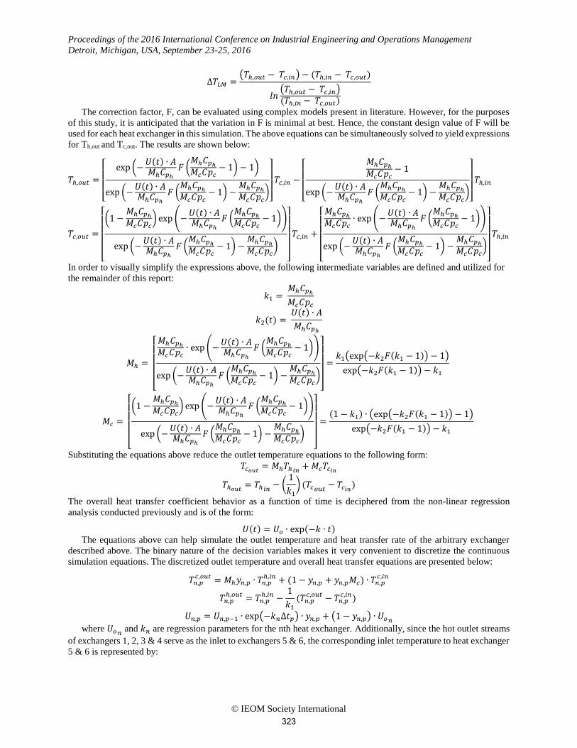
After many iterations of generating an industrially acceptable software for the problem, the team agreed on the

following architecture. The main elements of this architecture preside in the red boxes (software back-end). The

discussion will remain focused on these elements. While a lot of work was conducted on the front-end part of the

software (green boxes), a thorough discussion of these will remain out of scope for this report.

2.1 Data Manipulation and Filtration

In this portion of the software, data is collected from the plant historian and filtered to eradicate any erratic process

data (up to a year’s worth of data is considered). The primary data collected will usually be flow rate, temperature and

pressures at the inlet and outlet of each heat exchanger. The filtration methods being used in the preliminary version

of the software are moving average filters.

2.2 Fouling/OHTC Calculations and Statistical Regression

Modified data is then used to calculate OHTC and Fouling Factor. The mathematical essence of these calculations

is described in later sections. The calculated OHTC is then regressed as a function of run time for past runs for each

heat exchanger. The statistical regression parameters are an important input to the optimization model. Hence, the

statistical methods used must be very accurate.

2.3 Optimization Model Generation and Solution

This section of the software solves a pre-defined optimization model. The constraints of this model are subject to

the heat exchanger network at hand. However, some constraints depend on the statistical regression results for each

heat exchanger in the network. The objective function serves to minimize the operating cost. The output of this model

is the optimal cleaning schedule. More discussion on all components of the software will be presented in the context

of a case study below.

Figure 3. Software Architecture of the Proposed Solution

3. Model

3.1 Fouling & Overall Heat Transfer Coefficient Calculations

This section covers preliminary heat transfer theory utilized while calculating the Overall Heat Transfer

Coefficient (OHTC) from process data. A simple enthalpy balance on the two fluids yields:

321




�̇� = 𝑀ℎ ∙ 𝐶𝑝ℎ∙ (𝑇ℎ,𝑖𝑛 − 𝑇ℎ,𝑜𝑢𝑡(𝑡))

�̇� = 𝑀𝑐 ∙ 𝐶𝑝𝑐∙ (𝑇𝑐,𝑜𝑢𝑡(𝑡) − 𝑇𝑐,𝑖𝑛)

From heat transfer theory, the rate of heat transfer in the arbitrary heat exchanger above can be modelled as:

�̇� = 𝑈(𝑡) ∙ 𝐴 ∙ ∆𝑇𝐿𝑀 ∙ 𝐹 Solving for U (OHTC) yields:

𝑈(𝑡) =�̇�

𝐴 ∙ ∆𝑇𝐿𝑀 ∙ 𝐹=

𝑀ℎ ∙ 𝐶𝑝ℎ∙ (𝑇ℎ,𝑖𝑛 − 𝑇ℎ,𝑜𝑢𝑡(𝑡))

𝐴 ∙ ∆𝑇𝐿𝑀 ∙ 𝐹=

𝑀𝑐 ∙ 𝐶𝑝𝑐∙ (𝑇𝑐,𝑜𝑢𝑡(𝑡) − 𝑇𝑐,𝑖𝑛)

𝐴 ∙ ∆𝑇𝐿𝑀 ∙ 𝐹

The fouling factor at each time is easily computed through:

𝑓 =1

𝑈(𝑡)−

1

𝑈𝑐𝑙𝑒𝑎𝑛

However, it must be noted that Uclean is a function of the operating conditions (or inlet process conditions). In our

case, we will assume these to be fixed. Notice also that fouling factor is simply a modified representation of the OHTC.

It is merely used in our calculations, but it is useful to generate for monitoring purposes. We will only consider U or

OHTC for further calculations. Now that U can be calculated at various times during a run, statistical analysis can be

used to fit an empirical model. From a close analysis of the data, an exponential functions serves best to describe the

decaying U function. This can be expressed as:

𝑈(𝑡) = 𝑈𝑜𝑒−𝑘𝑡

where Uo and k are the regression parameters. Moving average filters are used to better filter the data at hand. This is

mathematically represented as:

𝑦𝑠(𝑖) =1

2𝑁 + 1(𝑦(𝑖 + 𝑁) + 𝑦(𝑖 + 𝑁 − 1) + ⋯+ 𝑦(𝑖 − 𝑁))

where, 𝑦𝑠(𝑖) is the smoothed value for the ith data point, 𝑁 is the number of neighbouring data points on either side

of 𝑦𝑠(𝑖).

3.2 Optimization model

The mixed integer non-linear programming (MINLP) optimization model intakes the results of the fouling analysis

and generates optimal cleaning decisions for each heat exchanger in the network, for a pre-defined time horizon. The

key decision variables are the cleaning of a specific heat exchanger in a specific period. Mathematically speaking, this

translates to:

𝑦𝑛,𝑝 = {1 (if heat exchanger n is in service during period p) 0 (if heat exchanger n is out of service during period p)

where n represents the number of heat exchangers in the network and p represents the number of periods. The time

horizon has been discretized into p periods, hence converting this continuous optimization problem into a discrete

one. This reduces the computational complexity and effort, and also accounts for logistical constraints. Additionally,

other decisions variables include: 𝑇𝑛,𝑝ℎ,𝑜𝑢𝑡

outlet temperature of the hot stream in heat exchanger n, with a given period

p, 𝑇𝑛,𝑝𝑐,𝑜𝑢𝑡

outlet temperature of the cold stream in heat exchange n, within a given period p, and 𝑈𝑛,𝑝 overall heat

transfer coefficient in heat exchanger n, within a given period p.

The simulation of the heat exchanger network is a critical component of the optimization model. As will be

described below, the statistical analysis of fouling data is a direct input to this component of the model. Consider a

single heat exchanger with a fixed heat transfer area A, hot inlet stream temperature and mass flow rate of Th,in, Mh

respectively and cold inlet stream temperature and mass flow rate of Tc,in, Mc. If the performance of the heat exchanger

is known through its overall heat transfer coefficient’s behavior as a function of time, then it is possible to solve for

the outlet temperature of both the streams. This is mathematically illustrated as follows, let �̇� denote total rate of heat

transfer between the hot and the cold streams. A simple thermodynamic heat balance between the two streams yield

the following equations:

�̇� = 𝑀ℎ ∙ 𝐶𝑝ℎ∙ (𝑇ℎ,𝑖𝑛 − 𝑇ℎ,𝑜𝑢𝑡)

�̇� = 𝑀𝑐 ∙ 𝐶𝑝𝑐∙ (𝑇𝑐,𝑜𝑢𝑡 − 𝑇𝑐,𝑖𝑛)

From heat transfer theory, the rate of heat transfer in the arbitrary heat exchanger above can be modelled as:

�̇� = 𝑈(𝑡) ∙ 𝐴 ∙ ∆𝑇𝐿𝑀 ∙ 𝐹

The Log-Mean Temperature used in the equation above is given by:

322




∆𝑇𝐿𝑀 =(𝑇ℎ,𝑜𝑢𝑡 − 𝑇𝑐,𝑖𝑛) − (𝑇ℎ,𝑖𝑛 − 𝑇𝑐,𝑜𝑢𝑡)

𝑙𝑛(𝑇ℎ,𝑜𝑢𝑡 − 𝑇𝑐,𝑖𝑛)(𝑇ℎ,𝑖𝑛 − 𝑇𝑐,𝑜𝑢𝑡)

The correction factor, F, can be evaluated using complex models present in literature. However, for the purposes

of this study, it is anticipated that the variation in F is minimal at best. Hence, the constant design value of F will be

used for each heat exchanger in this simulation. The above equations can be simultaneously solved to yield expressions

for Th,out and Tc,out. The results are shown below:

𝑇ℎ,𝑜𝑢𝑡 =

[ exp (−

𝑈(𝑡) ∙ 𝐴𝑀ℎ𝐶𝑝ℎ

𝐹 (𝑀ℎ𝐶𝑝ℎ

𝑀𝑐𝐶𝑝𝑐− 1) − 1)

exp (−𝑈(𝑡) ∙ 𝐴𝑀ℎ𝐶𝑝ℎ


𝑀𝑐𝐶𝑝𝑐− 1) −

𝑀ℎ𝐶𝑝ℎ

𝑀𝑐𝐶𝑝𝑐)]

𝑇𝑐,𝑖𝑛 −

[

𝑀ℎ𝐶𝑝ℎ

𝑀𝑐𝐶𝑝𝑐− 1




𝑀ℎ𝐶𝑝ℎ

𝑀𝑐𝐶𝑝𝑐)]

𝑇ℎ,𝑖𝑛

𝑇𝑐,𝑜𝑢𝑡 =

[ (1 −

𝑀ℎ𝐶𝑝ℎ

𝑀𝑐𝐶𝑝𝑐) exp (−



𝑀𝑐𝐶𝑝𝑐− 1))




𝑀ℎ𝐶𝑝ℎ

𝑀𝑐𝐶𝑝𝑐)

]

𝑇𝑐,𝑖𝑛 +

[ 𝑀ℎ𝐶𝑝ℎ

𝑀𝑐𝐶𝑝𝑐∙ exp (−







𝑀ℎ𝐶𝑝ℎ


]

𝑇ℎ,𝑖𝑛

In order to visually simplify the expressions above, the following intermediate variables are defined and utilized for

the remainder of this report:

𝑘1 = 𝑀ℎ𝐶𝑝ℎ

𝑀𝑐𝐶𝑝𝑐

𝑘2(𝑡) = 𝑈(𝑡) ∙ 𝐴

𝑀ℎ𝐶𝑝ℎ

𝑀ℎ =

[ 𝑀ℎ𝐶𝑝ℎ

𝑀𝑐𝐶𝑝𝑐∙ exp (−







𝑀ℎ𝐶𝑝ℎ


]

=𝑘1(exp(−𝑘2𝐹(𝑘1 − 1)) − 1)

exp(−𝑘2𝐹(𝑘1 − 1)) − 𝑘1

𝑀𝑐 =

[ (1 −

𝑀ℎ𝐶𝑝ℎ

𝑀𝑐𝐶𝑝𝑐) exp (−







𝑀ℎ𝐶𝑝ℎ


]

=(1 − 𝑘1) ∙ (exp(−𝑘2𝐹(𝑘1 − 1)) − 1)

exp(−𝑘2𝐹(𝑘1 − 1)) − 𝑘1

Substituting the equations above reduce the outlet temperature equations to the following form:

𝑇𝑐𝑜𝑢𝑡= 𝑀ℎ𝑇ℎ𝑖𝑛

+ 𝑀𝑐𝑇𝑐𝑖𝑛

𝑇ℎ𝑜𝑢𝑡= 𝑇ℎ𝑖𝑛

− (1

𝑘1

) (𝑇𝑐𝑜𝑢𝑡− 𝑇𝑐𝑖𝑛

)

The overall heat transfer coefficient behavior as a function of time is deciphered from the non-linear regression

analysis conducted previously and is of the form:

𝑈(𝑡) = 𝑈𝑜 ∙ exp(−𝑘 ∙ 𝑡) The equations above can help simulate the outlet temperature and heat transfer rate of the arbitrary exchanger

described above. The binary nature of the decision variables makes it very convenient to discretize the continuous

simulation equations. The discretized outlet temperature and overall heat transfer equations are presented below:

𝑇𝑛,𝑝𝑐,𝑜𝑢𝑡 = 𝑀ℎ𝑦𝑛,𝑝 ∙ 𝑇𝑛,𝑝

ℎ,𝑖𝑛 + (1 − 𝑦𝑛,𝑝 + 𝑦𝑛,𝑝𝑀𝑐) ∙ 𝑇𝑛,𝑝𝑐,𝑖𝑛

𝑇𝑛,𝑝ℎ,𝑜𝑢𝑡 = 𝑇𝑛,𝑝

ℎ,𝑖𝑛 −1

𝑘1

(𝑇𝑛,𝑝𝑐,𝑜𝑢𝑡 − 𝑇𝑛,𝑝

𝑐,𝑖𝑛)

𝑈𝑛,𝑝 = 𝑈𝑛,𝑝−1 ∙ exp(−𝑘𝑛∆𝑡𝑝) ∙ 𝑦𝑛,𝑝 + (1 − 𝑦𝑛,𝑝) ∙ 𝑈𝑜𝑛

where 𝑈𝑜𝑛 and 𝑘𝑛 are regression parameters for the nth heat exchanger. Additionally, since the hot outlet streams

of exchangers 1, 2, 3 & 4 serve as the inlet to exchangers 5 & 6, the corresponding inlet temperature to heat exchanger

5 & 6 is represented by:

323




𝑇5,𝑝ℎ,𝑖𝑛 =

(𝑦1,𝑝 ∙ 𝑇1,𝑝ℎ,𝑜𝑢𝑡 + 𝑦2,𝑝 ∙ 𝑇2,𝑝

ℎ,𝑜𝑢𝑡 + 𝑦3,𝑝 ∙ 𝑇3,𝑝ℎ,𝑜𝑢𝑡 + 𝑦4,𝑝 ∙ 𝑇4,𝑝

ℎ,𝑜𝑢𝑡)

3

𝑇6,𝑝ℎ,𝑖𝑛 =

(𝑦1,𝑝 ∙ 𝑇1,𝑝ℎ,𝑜𝑢𝑡 + 𝑦2,𝑝 ∙ 𝑇2,𝑝

ℎ,𝑜𝑢𝑡 + 𝑦3,𝑝 ∙ 𝑇3,𝑝ℎ,𝑜𝑢𝑡 + 𝑦4,𝑝 ∙ 𝑇4,𝑝

ℎ,𝑜𝑢𝑡)

3

The above equation assumes a constant mass flow rate distribution between Exchangers 1, 2, 3 and/or 4 during

normal operation. This is consistent with the previously listed assumption in the exchanger network operation. The

combination of all the algebraic equations in this section will easily allow us to simulate the heat exchanger network

performance during all periods p of interest. The mentioned operational requirements above will serve to generate

secondary constraints for this problem. Firstly, at least three heat exchangers out of the first four must always be in

service due to momentum transfer requirements. This yields:

𝑦1,𝑝 + 𝑦2,𝑝 + 𝑦3,𝑝 + 𝑦4,𝑝 ≥ 3

Secondly, at least one of the last two heat exchangers must always be in service due to heat transfer requirements.

This yields:

𝑦5,𝑝 + 𝑦6,𝑝 ≥ 1

Additionally, the outlet temperature of the system must be maintained under 93oC as per downstream process unit

requirements:

𝑦5,𝑝 ∙ 𝑇5,𝑝ℎ,𝑜𝑢𝑡 + 𝑦6,𝑝 ∙ 𝑇6,𝑝

ℎ,𝑜𝑢𝑡

𝑦5,𝑝 + 𝑦6,𝑝

≤ 93

As a final constraint, it is a good idea to ensure that no single heat exchanger is cleaned in two consecutive periods.

This is done using:

𝑦𝑛,𝑝 + 𝑦𝑛,𝑝−1 ≤ 1 Now that all the relevant constraints are defined, an acceptable objective function must be derived. From literature

review, it is apparent that many academic leaders in the field of scheduling prefer to minimize operating cost as their

objective. This makes conceptual sense and serves as our approach. The operating cost is comprised of two key

components in this case: 1) Cost of Heat Exchanger Cleaning: This is a self-explanatory cost. As the heat exchanger

is taken out of service, typically the contracting party doing the cleaning will require compensation for their services.

2) Cost of Energy (Heat) Losses due to Fouling: Fouling causes reduction in total heat exchanged during normal

operation, and additionally forces the heat exchanger to be ultimately taken out of service. This means that relative to

an ideal case without fouling, there is a substantial loss of potential heat transferred during normal and out-of-service

heat exchanger states. In our case, the Cost of Energy is essentially the additional amount of glycol (in $) required in

HX E & F per unit drop in energy per heat exchanger. The objective function can be mathematical described as:

𝑇𝑜𝑡𝑎𝑙 𝐶𝑜𝑠𝑡 = ∑ ∑(𝑄𝑐𝑙𝑒𝑎𝑛,𝑛 − 𝑄𝑛,𝑝)𝑦𝑛,𝑝 ∙ 𝐶𝑒𝑛𝑒𝑟𝑔𝑦 ∙ ∆𝑡

6

𝑛=1

𝑃𝑡𝑜𝑡𝑎𝑙

𝑝=1

+ ∑ ∑ 𝐶𝑐𝑙𝑒𝑎𝑛(1 − 𝑦𝑛,𝑝)

6

𝑛=1

𝑃𝑡𝑜𝑡𝑎𝑙

𝑝=1

where 𝐶𝑒𝑛𝑒𝑟𝑔𝑦 is the cost of unit energy and 𝐶𝑐𝑙𝑒𝑎𝑛 is the cost per cleaning. The combined model described in this

section is solved on GAMS using DICOPT. This enabled the generation of a heuristic solution for this non-convex

MINLP. Other solvers (which may have been more efficient) were not used for this project due to limited resources.

4. Case study

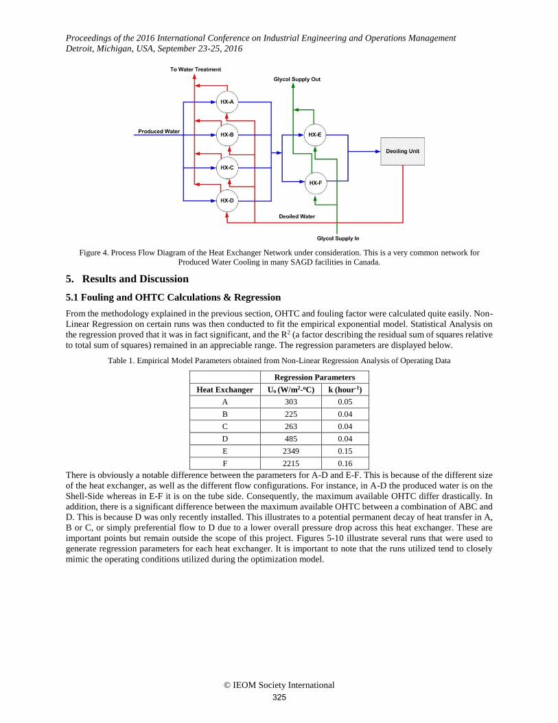
Figure 4 illustrates the HEN under consideration for this project. The network and subsequent data are associated

with a typical operating SAGD Facility. In essence, the produced water recovered from the thermal SAGD operation

is to be cooled before entering the de-oiling and water treatment units. This water is cleaned and converted to steam

before being injected back into the reservoir. There are 6 heat exchangers. The first set of four heat exchangers cool

the produced water with de-oiled water (cross heat exchange to maximize heat transfer). The second set of heat

exchangers (E & F) do the majority of the cooling using glycol as a cooling medium. All the heat exchangers are Shell

& Tube type. Additionally, the following operational constraints apply to this network: 1) at any given time, three heat

exchangers must be in service out of the first set of four (due to pressure drop constraints), 2) at any given time, one

heat exchanger must be in service out of E & F (due to heat transfer requirements), 3) the outlet temperature of the

Produced Water stream entering the Deoiling Unit must not exceed 93oC.

324




Figure 4. Process Flow Diagram of the Heat Exchanger Network under consideration. This is a very common network for

Produced Water Cooling in many SAGD facilities in Canada.

5. Results and Discussion

5.1 Fouling and OHTC Calculations & Regression

From the methodology explained in the previous section, OHTC and fouling factor were calculated quite easily. Non-

Linear Regression on certain runs was then conducted to fit the empirical exponential model. Statistical Analysis on

the regression proved that it was in fact significant, and the R2 (a factor describing the residual sum of squares relative

to total sum of squares) remained in an appreciable range. The regression parameters are displayed below.

Table 1. Empirical Model Parameters obtained from Non-Linear Regression Analysis of Operating Data

Regression Parameters

Heat Exchanger Uo (W/m2-oC) k (hour-1)

A 303 0.05

B 225 0.04

C 263 0.04

D 485 0.04

E 2349 0.15

F 2215 0.16

There is obviously a notable difference between the parameters for A-D and E-F. This is because of the different size

of the heat exchanger, as well as the different flow configurations. For instance, in A-D the produced water is on the

Shell-Side whereas in E-F it is on the tube side. Consequently, the maximum available OHTC differ drastically. In

addition, there is a significant difference between the maximum available OHTC between a combination of ABC and

D. This is because D was only recently installed. This illustrates to a potential permanent decay of heat transfer in A,

B or C, or simply preferential flow to D due to a lower overall pressure drop across this heat exchanger. These are

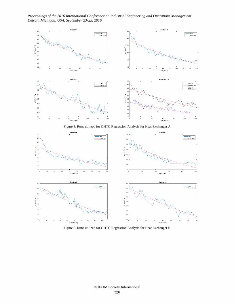
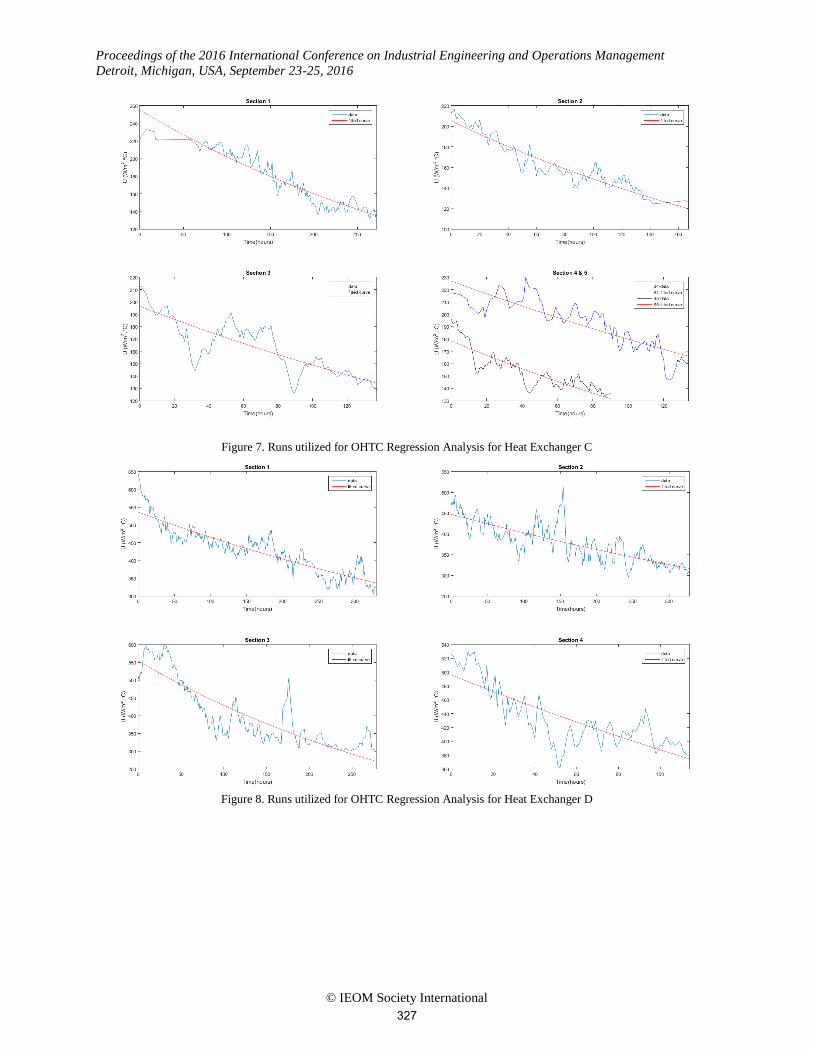
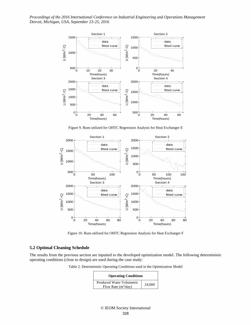
important points but remain outside the scope of this project. Figures 5-10 illustrate several runs that were used to

generate regression parameters for each heat exchanger. It is important to note that the runs utilized tend to closely

mimic the operating conditions utilized during the optimization model.

325




Figure 5. Runs utilized for OHTC Regression Analysis for Heat Exchanger A

Figure 6. Runs utilized for OHTC Regression Analysis for Heat Exchanger B

326




Figure 7. Runs utilized for OHTC Regression Analysis for Heat Exchanger C

Figure 8. Runs utilized for OHTC Regression Analysis for Heat Exchanger D

327




Figure 9. Runs utilized for OHTC Regression Analysis for Heat Exchanger E

Figure 10. Runs utilized for OHTC Regression Analysis for Heat Exchanger F

5.2 Optimal Cleaning Schedule

The results from the previous section are inputted to the developed optimization model. The following deterministic

operating conditions (close to design) are used during the case study:

Table 2. Deterministic Operating Conditions used in the Optimization Model

Operating Conditions

Produced Water Volumetric

Flow Rate (m3/day) 24,000

0 10 20 30500

1000

1500

Time(hours)

U (

W/m

2.

C)

Section 1

data

fitted curve

0 20 400

500

1000

1500

Time(hours)

U (

W/m

2.

C)

Section 2

data

fitted curve

0 20 40 600

500

1000

1500

2000

Time(hours)

U (

W/m

2.

C)

Section 3

data

fitted curve

0 20 40 60500

1000

1500

2000

Time(hours)

U (

W/m

2.

C)

Section 4

data

fitted curve

0 50 100500

1000

1500

2000

Time(hours)

U (

W/m

2.

C)

Section 1

data

fitted curve

0 50 100 1500

500

1000

1500

2000

Time(hours)

U (

W/m

2.

C)

Section 2

data

fitted curve

0 20 40 60 800

500

1000

1500

2000

Time(hours)

U (

W/m

2.

C)

Section 3

data

fitted curve

0 20 40 60 800

500

1000

1500

2000

Time(hours)

U (

W/m

2.

C)

Section 4

data

fitted curve

328




Produced Water Inlet

Temperature (oC) 125

Glycol Inlet Temperature

(oC) 30

Heat Transfer Area for HX -

A to D (m2) 642

Heat Transfer Area for HX -

E to F (m2) 732

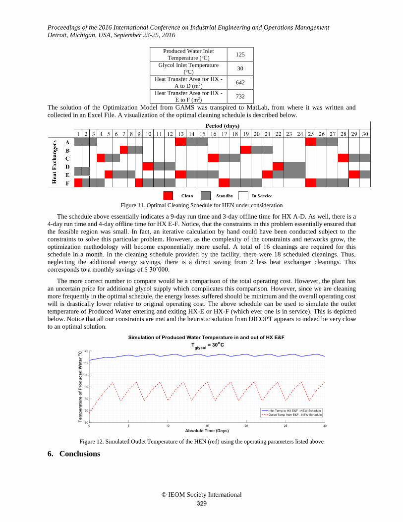
The solution of the Optimization Model from GAMS was transpired to MatLab, from where it was written and

collected in an Excel File. A visualization of the optimal cleaning schedule is described below.

Figure 11. Optimal Cleaning Schedule for HEN under consideration

The schedule above essentially indicates a 9-day run time and 3-day offline time for HX A-D. As well, there is a

4-day run time and 4-day offline time for HX E-F. Notice, that the constraints in this problem essentially ensured that

the feasible region was small. In fact, an iterative calculation by hand could have been conducted subject to the

constraints to solve this particular problem. However, as the complexity of the constraints and networks grow, the

optimization methodology will become exponentially more useful. A total of 16 cleanings are required for this

schedule in a month. In the cleaning schedule provided by the facility, there were 18 scheduled cleanings. Thus,

neglecting the additional energy savings, there is a direct saving from 2 less heat exchanger cleanings. This

corresponds to a monthly savings of $ 30’000.

The more correct number to compare would be a comparison of the total operating cost. However, the plant has

an uncertain price for additional glycol supply which complicates this comparison. However, since we are cleaning

more frequently in the optimal schedule, the energy losses suffered should be minimum and the overall operating cost

will is drastically lower relative to original operating cost. The above schedule can be used to simulate the outlet

temperature of Produced Water entering and exiting HX-E or HX-F (which ever one is in service). This is depicted

below. Notice that all our constraints are met and the heuristic solution from DICOPT appears to indeed be very close

to an optimal solution.

Figure 12. Simulated Outlet Temperature of the HEN (red) using the operating parameters listed above

6. Conclusions

329




In this study, it has been proven that a mathematical optimization approach can play a crucial role in minimizing

operating cost incurred from heat exchanger operation. Many plants have sufficient operating process data to make

data-driven scheduling decisions, backed by tested and proven optimization models. A savings of almost

$30’000/month is displayed from the use of such a scheme in the HEN considered throughout this project.

References

Bergman, T., & Lavine, A. S. (2011). Fundamentals of Heat and Mass Transfer. United States of America: John

Wiley & Sons, Inc.

Bott, T. R. (1995). Fouling of Heat Exchanger. Elsevier Science & Technology Books.

Clearly, E. (2011, November 13). Fouling Factor & Overall Heat Transfer Unit - U. Retrieved from Youtube:

https://www.youtube.com/watch?v=5dATY8Rxocc

Guomundsson, O. (2008). Detection of Fouling in Heat Exchanger. Reykjavik: University of Iceland.

Ibrahim, H. A.-H. (2012). Fouling in Heat Exchangers. Intech.

Jeronimo, M. (1997). Monitoring the Thermal Efficency of Fouled Heat Exchangers: A Simplified Method. New

York: Elsevier Science Inc.

Jin, Z. (2011). Planning the Optimum Cleaning Schedule Based on Simulation of Heat Exchanger under Fouling.

Zhengzhou: Wiley Periodicals Inc.

Shah, R. K., & Sekulic, D. P. (2003). Fundamentals of Heat Exchanger Design. Hoboken, New Jersey, United

States of America: John Wiley & Sons, Inc.

SMAIÈLI, F., ANGADI, D. K., HATCH, C. M., HERBERT, O., VASSILIADIS, V. S., & WILSON, D. I. (1999).

Optimization of Scheduling of Cleaning in Heat Exchanger Networks Subject to Fouling: Sugar Case

Study. Cambridge: Institution of Chemical Engineers.

Pogiatzis, T., Vassiliadis, V. S., & Wilson, D. I. (2011). An MINLP Formulation for Scheduling the Cleaning of

Heat Exchanger Networks Subject to Fouling and Ageing. Crete Island: www.heatexchanger-fouling.com

Biography

Ali Elkamel is a professor of Chemical Engineering at the University of Waterloo, Canada. He holds a B.S. in

Chemical and Petroleum Refining Engineering and a B.S. in Mathematics from Colorado School of Mines, an M.S.

in Chemical Engineering from the University of Colorado-Boulder, and a Ph.D. in Chemical Engineering from Purdue

University. His specific research interests are in computer-aided modeling, optimization, and simulation with

applications to the petroleum and petrochemical industry. He has contributed more than 250 publications in refereed

journals and international conference proceedings and serves on the editorial board of several journals, including the

International Journal of Process Systems Engineering, Engineering Optimization, International Journal of Oil, Gas,

Coal Technology, and the Open Fuels & Energy Science Journal.

Chandra Mouli Madhuranthakam is a professor of Chemical Engineering at the University of Waterloo, Canada.

His research interests include micro Process Systems Engineering - Design and Operation of Microfluidic reactors for

efficient synthesis of biodiesel and complex copolymers, Mixed Integer Nonlinear Programming and Global

Optimization Algorithms, Modeling and Optimal Control for Complex Biochemical Reaction Systems, Applied

Statistics- Modeling, Design of Experiments, and Parameter Estimation.

Mohamed Elsholkami is a Ph.D. student at the University of Waterloo. He earned his B.S. in Chemical Engineering

from the Petroleum Institute in Abu Dhabi, UAE. His research interests are in process systems engineering and

optimization.

Muhummad Bajwa, Matthew Aydemir, Terell Brown, and Dinesha Ganesarajan are students at the University

Of Waterloo.

330

http://www.heatexchanger-fouling.com/

Optimizing Cleaning Schedules of Heat Exchanger Networksieomsociety.org/ieomdetroit/pdfs/162.pdf · Consequently, Heat Exchanger Cleanings amount to a massive operating expenditure

Documents