Optimization of stochastic dynamic system with random ...

AN ABSTRACT OF THE THESIS

Man Hyung Lee for the degree of Doctor of Philosophy

in Electrical and Computer Enjineering presented on

February 25, 1983.

Title: OPTIMIZATION OF STOCHASTIC DYNAMIC SYSTEM WITH RANDOM

COEFFICIENTS

Redacted for PrivacyAbstract approved:

Professor Ronald R. Mohler

The problem of optimization of stochastic dynamic systems with

random coefficients is discussed. Systems with both Wiener pro-

cesses and uncertain random-process disturbances are dealt with in

this dissertation, and these include certain bilinear stochastic

systems. It is the purpose of this thesis to study the optimal con-

trol and, to some extent, state estimation of such bilinear sto-

chastic systems. By means of stochastic Bellman equation, the

optimal control of stochastic dynamic models with observable and

unobservable coefficients is derived.

The stochastic-system model considered is the observable system

with random coefficients that are a function of the solution of a

certain unobservable Markov process with information data. Under

the assumptions that the solution of the stochastic differential

equation for the dynamic model involved in the problem formulation results

in an admissible control and that the measurable information of all

random parameters depend on the conditional-mean estimate to the un-

observable stochastic process, the optimal control is a linear

function of the observable states and a nonlinear function of random

parameters.

The theory is then applied to an optimal-control design of an

aircraft landing with a bad weather situation, to the control

problem of longitudinal motion of an aircraft in wind gust, and to

nonlinear filtering and tracking of the maneuvering target. The

flare path compared with the desirable exponential-linear path pro-

vides a safe and comfortable landing for the optimal-control policy.

Using the decoupled feedback law of longitudinal aircraft motion,

it is shown that optimal-control policies for the elevator control

angle and the aileron control angle is synthesized with the attack

angle, the orientation rate of the aircraft and an unknown random

parameter. In the final example, a maneuvering target's state is

estimated. Here, a bilinear stochastic model is assumed such that

discrete velocity changes are at random times.

OPTIMIZATION OF STOCHASTIC DYNAMIC SYSTEMWITH RANDOM COEFFICIENTS

by

Man Hyung Lee

A THESIS

submitted to

Oregon State University

in partial fulfillment ofthe requirements for the

degree of

Doctor of Philosophy

Completed February 25, 1983

Commencement June 1983

APPROVED:

Redacted for PrivacyProfessor of Electrical and Computer Engineering in charge of major

Redacted for Privacy

Head of Dekirtment of Efgarical and Computer Engineering

Redacted for Privacy

Dean of Graduate

dchool

Date thesis is presented February 25, 1983

Typed by Jane A. Tuor for Man Hyung Lee

TO JONG SOOK, RAE WON, and JUNG MIN

With Love and Admiration

ACKNOWLEDGEMENTS

I want to express sincere thanks to my advisor, Professor

R. R. Mohler, for suggesting the problems and for his friendly

guidance and continuous encouragement during this work. Special

thanks are also due to Assistant Professor W. J. Kolodziej for

his comments and discussions.

I wish to acknowledge the support of the U.S. Office of Naval

Research through Contract No. N00014-81-K-084 to conduct this dis-

sertation.

Thanks to my grandparents, So Yoon and Gie Kun Choi, my

parents, Soon Jung and Sang June for their encouragement, dedication

and inspiration throughout my life, and for my future.

Finally and most importantly, with warmest regard, I thank my

B, H, J, parents-in-law, brothers and sisters for their love,

patience and support.

TABLE OF CONTENTS

Page1. Introduction 1

2. Optimal Control of a Stochastic System with RandomCoefficients 9

2.1. Optimal Control with Complete MeasurementInformation 9

3. Approximate Stochastic Models 20

3.1. Simple Approximation to Stochastic Modeling 21

3.2. Suboptimal Control of a Class of StochasticSystem with Unobservable Random Parameters 29

4. Simulation of Stochastic Control Processes with RandomCoefficients 39

4.1. Generation of the Wiener Process 41

4.2. Numerical Solution of a Nonlinear Partial Dif-ferential Equation 49

4.3. Application to an Aircraft Landing Problem 55

4.4. The Control Problem of Longitudinal Motion of anAircraft in Wind Gust 64

5. On Nonlinear Filtering and Tracking of Target 76

5.1. Modeling in Two-dimensional Space 76

5.2. On the Maneuvering Target Problem 80

5.3. Computer Simulation 86

6. Conclusions 95

REFERENCES 100

LIST OF FIGURES

Figure No. Title Page

4.1 Normalization curve of the pseudo-Wienerprocess 44

4.2 Solutions of the Riccati equations for(a) A0=3.75, Al=1.50, (b) A0=3.2, Al=1.20,(c) Ao=2.5, Al=1.0, (d) A0=2.0, A1=0.75,(e) A0=1.5, A1=0.5 54

4.3 Optimal control law and suboptimal controllaw for example 4.2 56

4.4 Realization of xt under optimal and sub-optimal conditions for example 4.2

4.5 The optimum descent rate of the aircraftlanding process

4.6 The optimal control law of the aircraftlanding process

4.7 The optimal trajectory of the aircraftlanding process

57

61

62

63

4.8 Solutions of Riccati-like-equation for thecontrol of longitudinal motion of an air-craft 71

4.9 The optimum trajectory of (a) observable and(b) unobservable angle of attack 72

4.10 The optimum trajectory of (a) observable and(b) unobservable orientation range rate 73

4.11 Optimal control of elevator control angle for(a) observable states and (b) unobservablestates

4.12 Optimal control of aileron control angle for(a) observable states and (b) unobservablestates

5.1 Geometrical definition of vector tracking

5.2 Ranges of x-direction of (a) extended Kalmanfilter, (b) truncated second-order filter,and (c) reference trajectory for constantspeed of target

74

75

76

89

Figure No.

LIST OF FIGURES - CONTINUED

Title Page

5.3 Ranges of y-direction of (a) extended Kalmanfilter, (b) truncated second-order filter,and (c) reference trajectory for constantspeed of target

5.4 Ranges of (a) extended Kalman filter, (b)

truncated second-order filter, and (c)reference trajectory for constant speed oftarget

5.5 Ranges of x-direction of (a) extended Kalmanfilter, (b) truncated second-order filter,and (c) reference trajectory for maneuveringtarget

5.6 Ranges of y-direction of (a) extended kalmanfilter, (b) truncated second-order filter,and (c) reference trajectory for maneuveringtarget

5.7 Ranges of (a) extended Kalman filter, (b) trun-cated second-order filter, and (c) referencetrajectory for maneuvering target

90

91

92

93

94

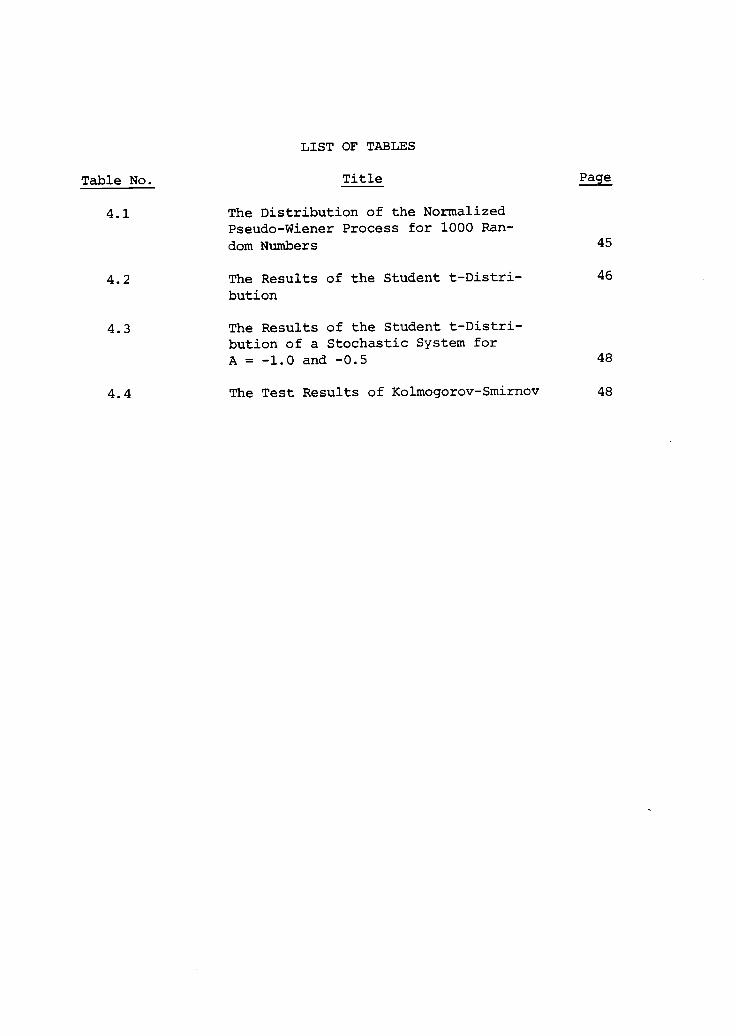
Table No.

LIST OF TABLES

Title Page

4.1 The Distribution of the NormalizedPseudo-Wiener Process for 1000 Ran-

dom Numbers 45

4.2 The Results of the Student t-Distri- 46

bution

4.3 The Results of the Student t-Distri-bution of a Stochastic System forA = -1.0 and -0.5 48

4.4 The Test Results of Kolmogorov-Smirnov 48

OPTIMIZATION OF STOCHASTIC DYNAMIC SYSTEM WITHRANDOM COEFFICIENTS

1. INTRODUCTION

Most of the results in stochastic dynamic control and filter-

ing theory were obtained with the assumptions that the process

under some special considerations satisfy stochastic differential

equations. Unfortunately, very little is known about optimal con-

trol theory for processes governed by general stochastic differ-

ential equations. In this area, most of the contributions are

made by Fleming [1,2,3,4], Kushner [5,6], Wonham [7,8,9], Balakrish-

nan [10,11], Benes [12,13], Rishel [14,15], Bismut [16,17,18], Davis

[19,20,21,22,23], Eliott [24,25], Haussman [26,27], Variya [28],

Kolodziej [29], and Mohler and Kolodziej [30,31].

The status of continuous-time stochastic theory was summarized

in Fleming's 1969 survey paper [3] and also introduced in his book

[4] concerning the control of completely observable diffusion pro-

cesses. In regard to problems with partial observation, possibly

the most significant result was from Wonham's formulation of the

separation principle [7] using the stochastic version of Bellman's

dynamic programming which Wonham proved by reformulating the problem

as one of the complete observations with the state being the con-

ditional mean estimate produced by the Kalman-Bucy filter.

The dynamic-programming method is a useful approach in sto-

chastic control. However, these conditions under dynamic program-

ming are so much weaker than those required in deterministic control.

2

The dynamic-programming approach, while successful in many appli-

cations, suffers from many limitations. An immediate one is that

the controls have to be smooth functions of the state in order that

the stochastic differential equation has a solution in the Ito

sense.

In problems of engineering design, it is often necessary to

choose component values from an admissible set in addition to

choosing control from an admissible class, such that the final

product has the best performance in some appropriate sense. A

typical example is the stochastic dynamic system with random co-

efficients which has attracted the attention of numerous authors

[9,15,16,17,18,29,30,31,32,33,34,35,36,37]. One of the most formal

approaches to stochastic control of such systems was presented by

Bismut on convex analysis. Bismut solved a very general

class of linear, quadratic, finite-dimensional, stochastic-control

problems with random coefficients in which both state and control

dependent noises are admitted, and he also discussed the necessary

condition of stochastic optimality. Bensoussan and Voit [38] have

considered optimal control problems for the stochastic evolution

equation with deterministic operator-valued coefficients and have

developed a separation principle for the problem. Recently, Ahmed

[35] has solved the optimal-control porblem of the stochastic evolu-

tion equation and has considered a random operator Riccati equation

and backward stochastic evolution equation. For the stochastic

discrete-time system, the linear-quadratic optimal control has been

investigated by Athans, et al., [36] and Ku, et al., [37].

3

Kolodziej [29], Mohler and Kolodziej [30,31] presented an

alternate approach to the stochastic control of a class of linear

stochastic systems with random coefficients. Kolodziej solved the

problem of optimal control using dynamic programming. He also dis-

cussed the separation of filtering and control which was proven

by reformulating the problem as one of complete observations and

the control problem as an optimal regulator, which is a linear func-

tion of the unobservable part of the process and a nonlinear function

of the observable parts. Sufficient conditions for optimal control

were expressed through the existence of a bounded solution to a cer-

tain Cauchy problem for a parabolic type of partial differential

equation. He assumed that the random process is conditionally

Gaussian, i.e., the conditional distributions on the given random

process are Gaussian (P-a.s.).

This dissertation presents the problem of the optimal control

of stochastic differential equations with random coefficients. Sys-

tems with both Wiener processes and uncertain random process dis-

turbances are dealt with in this study, and these include certain

bilinear stochastic systems [31,39,40,41]. It is the objective

of this thesis to study the optimal control and, to some extent,

state estimation of such bilinear stochastic systems.

In general, it is difficult for a natural stochastic system

to keep the conditional-Gaussian distribution of some states. Hence,

Chapter 2 of this thesis considers observable stochastic-control

systems with observable finite-dimensional random coefficients.

Here, the stochastic Bellman equation to diffusion processes is

4

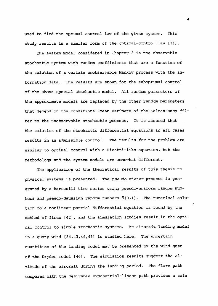
used to find the optimal-control law of the given system. This

study results in a similar form of the optimal-control law [31].

The system model considered in Chapter 3 is the observable

stochastic system with random coefficients that are a function of

the solution of a certain unobservable Markov process with the in-

formation data. The results are shown for the suboptimal control

of the above special stochastic model. All random parameters of

the approximate models are replaced by the other random parameters

that depend on the conditional-mean estimate of the Kalman-Bucy fil-

ter to the unobservable stochastic process. It is assumed that

the solution of the stochastic differential equations in all cases

results in an admissible control. The results for the problem are

similar to optimal control with a Ricatti-like equation, but the

methodology and the system models are somewhat different.

The application of the theoretical results of this thesis to

physical systems is presented. The pseudo-Wiener process is gen-

erated by a Bernoulli time series using pseudo-uniform random num-

bers and pseudo-Gaussian random numbers N(0,1). The numerical solu-

tion to a nonlinear partial differential equation is found by the

method of lines (42], and the simulation studies result in the opti-

mal control to simple stochastic systems. An aircraft landing model

in a gusty wind [34,43,44,45] is studied here. The uncertain

quantities of the landing model may be presented by the wind gust

of the Dryden model [46]. The simulation results suggest the al-

titude of the aircraft during the landing period. The flare path

compared with the desirable exponential-linear path provides a safe

5

and comfortable landing for the optimal control policy. The longi-

tudinal motion of aircraft in a gusty wind given in Chapter 4 can

be obtained by theoretical results of Chapter 3.

The decoupled feedback law of longitudinal motion of aircraft

which included unknown quantities and is also subject to uncertain

noise is discussed. Using an approximate stochastic model of longi-

tudinal aircraft motion for the worst situation, it is shown that

optimal control policies for the elevator control angle and the

aileron control angle is synthesized with the attack angle, the

orientation rate of aircraft, and an unknown random parameter. The

simulation results are compared with the assumptions of observable

and unobservable cases, respectively.

In Chapter 5, anti-submarine target-motion analysis on

nonlinear filtering and tracking is presented. A common method

in the target-tracking problem [47,48,49,50,51,52] is to model the

target dynamics in a rectangular-coordinate system which results in

a linear set of state equations because of the assumption that drag

forces are linear relationships in states or are neglected. However,

the drag forces are proportional to velocities squared in each tar-

get motion's directions [53,54]. Hence, a more appropriate mathe-

matical model is derived for the consideration of nonlinear target

dynamics underwater. With this model, this chapter compares perform-

ances between an extended Kalman filter and a truncated second-order

nonlinear filter as applied to bearing-only-target tracking. In the

existence of a maneuvering of target, many authors [47,48,49,50,55,

56,57,58,59,60,61,62,63] have proposed compensators for the Kalman

6

filter for adaptation to maneuvering situation. The target motion

equation for estimates of the vehicle maneuvering performance may

be represented by a bilinear stochastic system which has jumps so

that between jumps it remains in specific states at random time T.

The stochastic process involved in the maneuver is discussed. The

last section shows the filtering and control problem as the adaptive

control is a function of random time T and the new extended states

by solving certain Riccati equations.

7

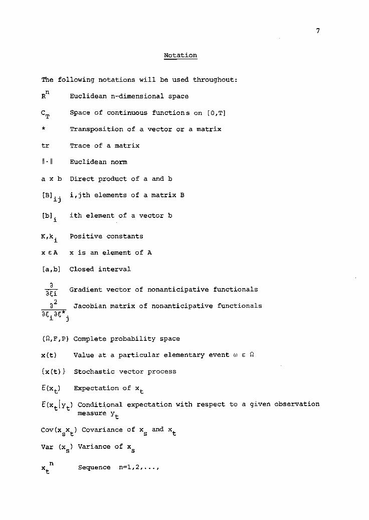
Notation

The following notations will be used throughout:

Rn

Euclidean n-dimensional space

CT

Space of continuous functions on [0,T]

Transposition of a vector or a matrix

tr Trace of a matrix

H-H Euclidean norm

a x b Direct product of a and b

[B].. i,jth elements of a matrix B13

[b].1

ith element of a vector b

K,k.1

Positive constants

x eA x is an element of A

[a,b] Closed interval

3

ai Gradient vector of nonanticipative functionals

32

Jacobian matrix of nonanticipative functionalsDE.3E=.

(R,F,P) Complete probability space

x(t) Value at a particular elementary event w

{x(t)} Stochastic vector process

E(xt) Expectation of xt

E(xtlyt) Conditional expectation with respect to a given observationmeasure y

t

Cov(xsxt) Covariance of x

sand x

t

Var (xs) Variance of x

s

nxt Sequence n=1,2,...,

8

HAH The Euclidean norm is defined as A being a vector ora matrix as follows

HAH2 = tr(AA*);

Ft

Sub-a-field of F

Yt

a-algebra {ys, 0 < s<t} generated by observable sto-chastic process {yt, t e [0,T]}

Z. a-algebra {x and ys, 0 < s < t} generated by the observ-able stochasEic process (Tc

tand yt, t E [0,T])

8(t,) Measurable nonanticipative functional parameter

inf infimum

xdx

Denotes -d-.E

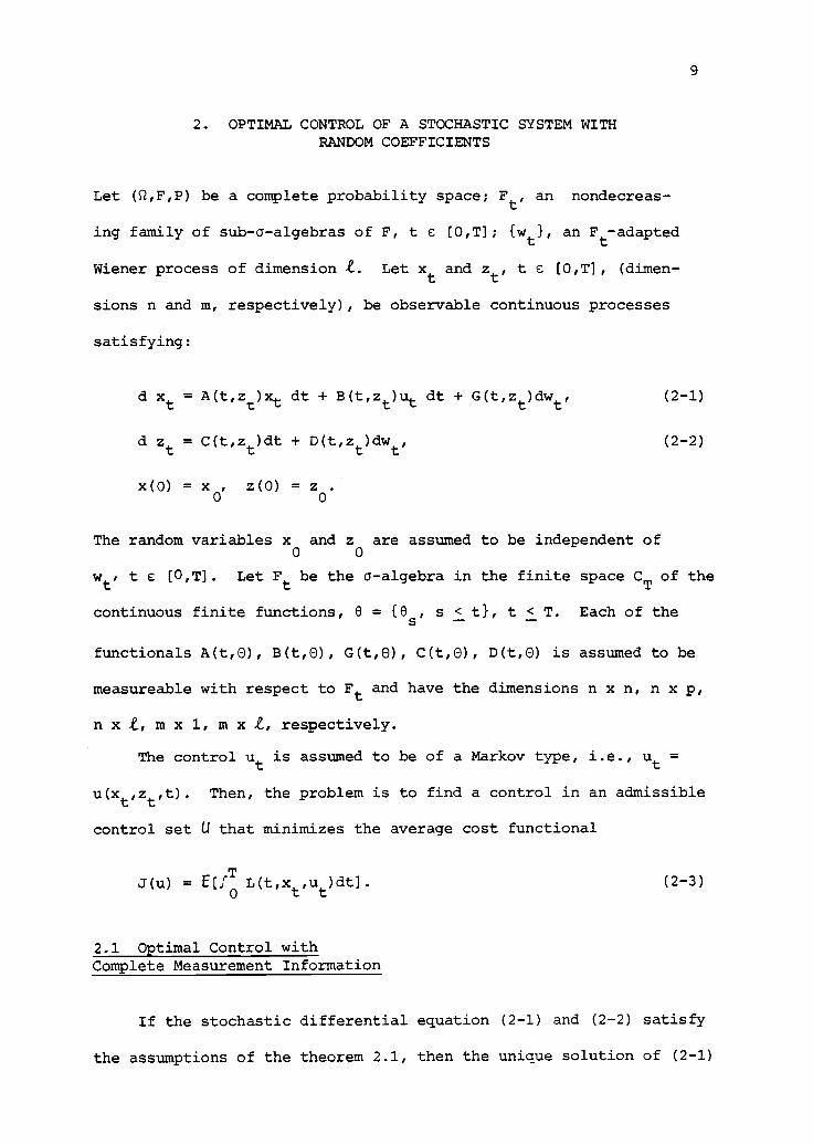
2. OPTIMAL CONTROL OF A STOCHASTIC SYSTEM WITHRANDOM COEFFICIENTS

Let (Q,F,P) be a complete probability space; Ft, an nondecreas-

ing family of sub-a-algebras of F, t e [O,T]; {wt }, an Ft-adapted

Wiener process of dimension £. Let xt and zt, t e [O,T], (dimen-

sions n and m, respectively), be observable continuous processes

satisfying:

d xt = A(t,zt)xt dt + B(t,zt)ut dt + G(t,zt)dwt,

9

(2-1)

d zt= C(t,z

t)dt + D(t,z

t)dw

t, (2-2)

x(0) = x0, z(0) = zo

.

The random variables x and z are assumed to be independent of0 0

wt. t e [0,T]. Let Ft be the a-algebra in the finite space CT of the

continuous finite functions, 8 = {es, s < t }, t < T. Each of the

functionals A(t,0), B(t,0), G(t,0), C(t,0), D(t,0) is assumed to be

measureable with respect to Ft and have the dimensions n x n, n x p,

n x £, m x 1, m x £, respectively.

The control ut is assumed to be of a Markov type, i.e., ut =

u(xt,zt,t). Then, the problem is to find a control in an admissible

control set U that minimizes the average cost functional

J(u) = E[ioL(t,x

t,u

t)dt].

2.1 Optimal Control withComplete Measurement Information

(2-3)

If the stochastic differential equation (2-1) and (2-2) satisfy

the assumptions of the theorem 2.1, then the unique solution of (2-1)

10

and (2-2) exists [47,48].

Theorem 2.1 Let A(s,n), B(s,n), G(s,n), C(s,n), D(s,n),

s e [0,T] be Ft-measurable functionals, C(s,n), D(s,n) satisfy

the Lipschitz condition, and IA(t,n)1 <k1 <co, 113(t,n)1 <k2 < co,

T

fo

IIG(t,11)112 <.k3

< co. Then, if x° is a FO- measurable random

* *z0

vector, E[x0x0] + ETz

0z0] <co, the stochastic differential equa-

tions (2-1) and (2-2) have the unique solutions, i.e., xt

, zt

are

Ft-adapted and xt, zt are given by

(2-4)

xt

= x00

+ft A(s,zs

) xsds + f

oB(s,z

s)u

sds + to G(s,z

s)dw

s,

zt = z0 f0 C(s,zs)ds + f

oD(s,z

s)dw

s(2-5)

The above integrals are defined in the Ito sense. Here k1, k

2k3

are positive constants.

Proof The proof is omitted. The reader is referred for

details to Liptser and Shiryayev [47,48].

Now consider the problem of optimal control of xt for t e [0,T]

based on the complete observations of xtand z

t.The observable

states xt

and ztare the solution of equations (2-1) and (2-2),

respectively. The problem is to choose a control law ut so as to

minimize the cost functional (2-3).

For the solution of the optimal control, the following assump-

tions are introduced [29,31]:

1) Assumptions of the theorem 2.1 are satisfied.

2) L(t,xt,ut

) = xtQ(t,z

t)x

t+ u

tR(t,z

t)ut

where for n e Rm, t e [0,T], Q(t,n) is a nonnegative

definite matrix, and R(t,n) is uniformly positive

11

definite, i.e., elements of its inverse are uniformly

bounded measurable functions,.

3) The control ut e U satisfies

IT

E[Hut

II

2] dt < co,

0

ut= u(t,x

t,z

t),

and is such that (2-1) has a unique solution.

Let s c [0,T] be the initial time; xs= x0, the initial state,

utcU, and xt, the corresponding response of the system (2-1).

The conditional remaining cost on the time s = 0 is defined by

Wu(s,x

s,z

s) = E[f

oL(t,x

t,z

t,u

t)dt I xs=x0 ,z

s=zo ] , (2-6)

as the expected cost corresponding to the control ut and initial

state x0 and z0. Here, T is a fixed terminal time and L(,-,-) is

a bounded measurable function. The problem is to minimize J(u) on

U.

Let

a(t,n)A=

G(t,n) G (t,n)

p(t,n) G (t,n)

G(t,n) D

*p(t,n) D

(t,n)

(t,n)

and assume that a(t,n) is uniformly positive definite over t e (0,T),

.

n e Rm

, i.e.,

n+m>.E. a.. (t,n)y.y. klyy*I, k > 0,

1,3 13 1

for all y 6 Rn+m

. This essentially states that noise enters every

component of (2-1), whatever the coordinate system.

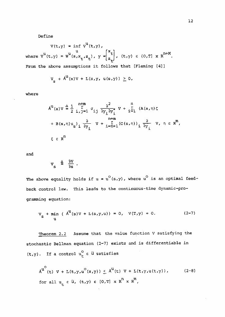
Define

V(t,y) = inf Vu(t,y),

where Vu(t,y) = W

u(s,x

t,z

t), Y = ztI, (t,y) E (0,T] x R

n+M.

From the above assumptions it follows that [Fleming [4]]

where

and

Vs

+ Au(s)V + L(s,y, u(s,y)) > 0,

nA 1 a

2

Au

n+m(s)V =

2* V + E (A(s,n)

i,j=1 ij ay.ay. i=1

n+ma m

+ B(s,n)us

)

i 8aV + i=nE

+1(c(s,n))

i 17..

V, n E R ,.yi

R

A ayVs

=as

The above equality

back control law.

gramming equation:

12

holds if u = uo(s,y), where u

ois an optimal feed-

This leads to the continuous-time dynamic-pro-

Vs+ min ( A

u(s)v + L(s,y,u)) = 0, V(T,y) = 0.

Theorem 2.2

(2-7)

Assume that the value function V satisfying the

stochastic Bellman equation (2-7) exists and is differentiable in

(t,y). If a control uo e U satisfies

Au (t) V + L(t,y,e(s,y)) < Au(t) V + L(t,y,u(t,y)),

for all ut

U, (t,y) e [0,T] x Rn x Rm

(2-8)

13

ithen utis an optimal control.

Proof Let uts U be any control and y = the correspondingt z

t

trajectory. From Bellman's principle of optimality and the Taylor

expansion on V,

V(t,x ,z ) = min CL(t,xt'

zt'

ut)(5 + V(t,x

t,z

t)+

DV(t,x ,z )(5

u Ute

+ Au(t) V(t,xt,zt) + 0(5)},

where any 6 e (0, T-t). Now dividing by 6 and let &+0, then

3V+ min (Au(t)V(t,x

t,zt

) + L(t,xt,zt,ut

) = 0 (2-9)

utcU

V(T,xT,zT

) = 0.

Equation (2-9) is the Bellman-Hamilton-Jacobi, BHJ, equation derived

heuristically above (2-7). Then from (2-9)

DV

at(t,x z ) + Au(t)V(t

'

xt'

zt

) + L(t'

x z ut

) > 0.

Thus, using Ito's formula it follows that

Tt- (v(t,xt,zt)) =av

(t,xt,zt) + Au(t) v(t,xt,zt) >

(2-10)

-L(t,xt,z

t,ut).

Taking the expectation of the both sides of (2-10) and integrating,

the following equation is obtained.

dVE(V(T,x

T,zT

) - V(0,x z 0)] =T

(t,xt,zt)dtdt

T

>-oL(t,x

t,z

t,ut)dt.

(2-11)

Since V(T,xT,zT

) = 0, this shows that the following inequality holds:

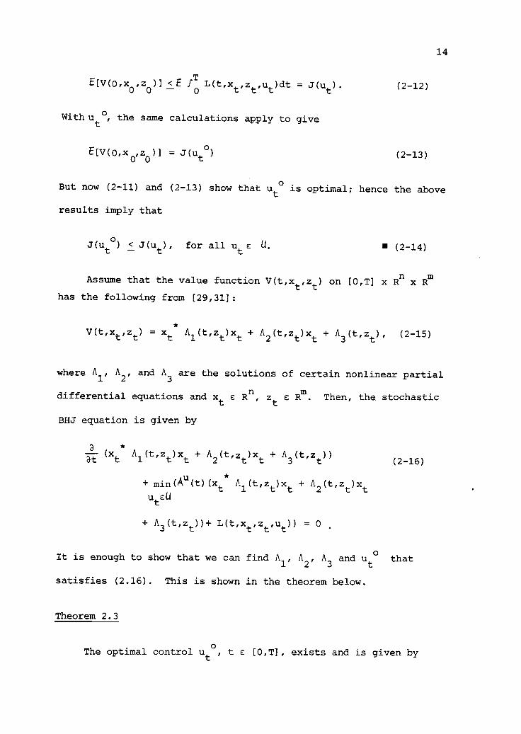
E[V(0,x0,z

0 0)] <E f L(t,x

t,zt,u

t)dt = J(u

t).

With ut°, the same calculations apply to give

E[V(0,x0,z

0)] = J(u

t0)

(2-12)

(2-13)

14

But now (2-11) and (2-13) show that ut

ois optimal; hence the above

results imply that

J(ut°) < J(ut), for all ut E U. (2-14)

Assume that the value function V(t,xt,zt

) on [0,T] x Rn x Rm

has the following from [29,31]:

V(t,xt,zt) = xt Al (t,zt)x

t+ A

2(t,z

t)xt+ A

3(t,z

t), (2-15)

where A1

, A2

, and A3are the solutions of certain nonlinear partial

differential equations and xt a Rn, zt E Rm. Then, the stochastic

BHJ equation is given by

at(xt Al(t,zt)x

t+ A

2(t,z

t)x

t+ A

3(t,z

t))

min(Au(t)(xt Al(t,zt)xt + A2(t,zt)xt

utEU

+ A3(t,z

t))+ L(t,x

t,zt,u

t)) = 0

(2-16)

It is enough to show that we can find Al , A2 , A3 and ut

othat

satisfies (2.16). This is shown in the theorem below.

Theorem 2.3

The optimal control uto

t e [0,T], exists and is given by

15

uto 1

= -R (t,zt)B (t,z

t)(A

l(t,z

t)xt 2

1+ A

2(t,z

t)), (2-17)

if there exist the nonnegative definite symmetric matrices Al and A2

satisfying the following nonlinear partial differential equations:

A +*A1 -1 *

Ai + C* a

aztAi

2* a+ 2 tr(DD

az 3z*)A

1= 0, (2-18)

t t

* a * 2

A2 + A2A - A2BR-1

B*Al + C A, + tr(DD *)A2

azt` t t

a

+ 2(GD*7" ) *A1 = 0,

t

A1(T,z

T) = 0, A

2(T,z

T) = 0, zt e Rm ,

(the argument (t,zt) is omitted for bervity).

Proof. Using the dynamic-programming equation (2-16), it

follows that

DA2

aA3

n nx

*3 Al

x + x + + min (-1 ( .E ( .E a (-2-)t at t at t at 2 1=1 3=1 ij axt ax

tj

ute

n+m n+m na a

+. E a. ) + E ( E a. (77--)3=n+1 ij axt i axt j i=n+1 j=1 13 dzt i axt j

n+m+. E

ia) ( ).)).(x

t

*A

1xt

+ A2x + A

3)

3=n+l j azt

azt

3 t

n+ .E

1(AX

t1311

t)

i(-)

j*((

t

*A

lxt+ A

2Xt

A3)1=axt

(2-19)

m * *

+i i2 (C) (az

a

t

)

i(x t* Alx

t+A2x

t+A3 ) +x

tQx

t+u

tRu

t) = 0.

=l

The equation (2-19) can be represented by the following equation:

16

*" 1n

ax Ax +Ax +A +1(( a. ( ) (a ) +t it 2 t 3 2 ,j=1 ij ax i ax

t t

n+mE a .( ) ( ) ) (xAx+Ax+A) +

i,j=n+113 az

ti az

tj t 1 t 2 t 3

n n+m n+m na a a

(.E E a + E Eazt

i(ax

t2

i-)

j)

i=1 j=n+1j ax

ti'az j ij

i=n+1 j=1

m.(xtAl

xt

+A2xt)) + E (C) (a ) (x t*Aixt + A3) + xt* Qx

ti=1

n+ min( E (Bu

3(x

*Ax + A x ) + u*Ru ) = 0- (2-20)

u EU i=1tiax

titlt 2t t t

Only the last term in (2-20) includes the control, and

E (Bu ) e-a

(x A (t,z )x + A (t,z )x ) + ut

R(t,zt t)u )

i=1tiax

ttl tt 2 tt

-1= Olt + R (t,z )(B (t,z

t)A

1(t,z

t)x

t 2+1 *

B (t,zt)A

2(t,z

t)))

*-12(t,z

t)(u

t+ R

-1(t,z )(B (t,z

t)A

1(t,z

t)x

t+

1B (t,z

t)A

2(t,z

t)))

- (R-1

(t,zt)(B

*(t,z

t)A

1(t,z

t)x

t 2+1

B*(t,z

t)A

2(t,z

t))

*

-1 1 *R(t,z )(B (t,z

t)A

1(t,z

t)x

t+ -2- B (t,z

t)A

2(t,z

t)). (2-21)

It follows that the minimum is obtained at

ut

o=

1(t,z )B

*(t,z

t)(A

1(t,z

t)xt

+1

A2(t,z

t)).

Substituting (2-22) into (2-20) gives

(2-22)

* a2

t

* a *2

x(9 t 1

+ A*Ai + AlA +Q+C-,=.- Al + tr(DD

- 12

a- A

1BR B

*Al)xt + e5TA2 + A2A + C

* a

A2 + tr(DD*

t

*)A2

t

a

+ 2(GD,---)

*A - A BR B

*A )x + (2-- A + C

*---

1 t 9t 3 3 3azt

1 2

1

ztA

12

+ tr(DD*------r)A + tr(GG

*)A

1) = 0.

2 9zt3z

t3

17

(2-23)

Because (2-23) has to be established for all xtc Rn, Al , A2 , A3

must satisfy

and

9A1 a

AA1-AA-Q+ A

1BR

-1B*A1-C

*Al

at° t

1 * 2

-2- tr(DD az--5-z---w)A1,

t t3A

2 * a 2

= -A A + A2BR

1B*A - C

* a 1A - tr(DD )A2

at 2 1 9zt

2 2t t

2(GD* *

A ,

9zt

1

IA3 * D

2*A -

1tr(DD -----w)A - tr(GG )A= -C

at azt

3 2 3 zt 9 3 1,zt

A1(T,z

T) = 0, A

2(T,z

T) = 0, A

3(T,z

T) = 0,

respectively.

The solutions A1(t,n) and A

2(t,n) to the above Cauchy problem can

be shown to be nonnegative definite and uniformly bounded for all

(t,n) e [0,T] x Rm [29].

Mohler developed bilinear stochastic systems that are the

18

diffusion models for migration of people, biological cells, etc.,

[30,31,66,67,68]. The system equation in (2-1) is a class of

coupled bilinear stochastic equations. In this particular case,

the optimal control of the bilinear stochastic system of diffusion

processes (2-1) and (2-2) is given by (2-17). The following examples

belong to the class of coupled bilinear stochastic systems.

Example 2.1 If A(t,zt

) = 0, G(t,zt

) = G(t), then the equation

(2-1) is

dxt= B(t,)u

tdt + G(t)dw

t'x(0) = xo c Rn; (2-24)

where B(t,) is composed of unknown coefficients. Such uncertain

parameters may be regarded as additional state variables. These

additional state variables with uncertain gain might be approximated

by

dzt

= C(t,zt)dt + D(t)dwt, z(0) = zo R . (2-25)

If B(t,) = B(t)zt

, (2-24) is bilinear in z and ut

, and the system

has an extended state with Rn+m

. At this point the problem of un-

certain parameter becomes a parameter-identification problem and

the system equation is a bilinear stochastic differential equation.

An aircraft landing process [44] may be represented by this type of

bilinear stochastic equation.

Example 2.2

Consider the stochastic differential equation with the random

coefficients,

dxt

= A(t,zt)x

tdt + B(t,z

t) u

tdt + G(t)dw

t

1

19

(2-26)

where state xt e Rnis observable and uncertain disturbance process

R izt E R is partially observable; and

dzt = zt dt + D(t) dwt

with the observation

2

dyt

= F(t)ztdt + H(t) dw

t

3.

The problem of optimal control of (2-26) under the given information

will be discussed in Chapter 3.

Comment: The optimal control of partially observable state xt was

discussed by Kolodziej [29]. There exists the optimal filter in

the conditionally Gaussian case. The form of optimal control law

of this particular case is the same as the equation (2-17).

The stochastic dynamic model in (2-26) may be approximated in

certain ways for c- algebra Ytgenerated by observation {y

t,t E [0,T]}

or a-algebra Ztgenerated by observation {x

t,y

t,t E [0,T]}. If there

is an exact solution to the problem of finite conditional estimate

E(

xt] the stochastic dynamic equation may provide optimal control

tt '

of (2-26). If A(t,zt

) and B(t,zt

) in (2-26) are replaced with

E[A(t,zt)lYt], E[B(t,zt)IYt], the problem of sub-optimal control

is similar to that introduced at the beginning of this chapter.

20

3. APPROXIMATE STOCHASTIC MODELS

Formulating a mathematical stochastic model for the dynamic

behavior of a physical system is in terms of the evolution of the

state xt, t E [0,T], of the system which is a stochastic process

defined on some complete probability space (S2,F,P) under the in-

fluence of control ut

and disturbances ztas the solution of the

stochastic differential equation,

(3-1)

dxt= A(t,z

t)xtdt + B(t,z

t)u

tdt + G(t,z

t)dw

t

1, x(0) = x0,

0

and xt

is an observable process and wt

1is a Wiener process. Assume

that this stochastic system has disturbances as the solution of a

stochastic differential equation

dzt

= C(t)ztdt + D(t)dw

t

2z(0) = z0,

with observation

dyt

= F(t)ztdt + H(t)dw

t

3,

(3-2)

(3-3)

where zt is unobservable and wti

i, = 1,2,3, are mutually independ-

ent Wiener processes of dimensions ti, respectively. The matrices

A, B, G, C, D, F, and H have the dimensions n x n, n x p, n x £1,

m x m, m x £2, k x m and k x £3, respectively. Assume that A(t,zt),

B(t,zt), and G(t,z

t) of (t,z

t) E [0,T] x R

mare Borel measurable.

Let Zt be the a-algebra generated by {xs

and ys

, 0 < s < t }.

The control utof dimension P is assumed to be Z

tmeasurable for

every t c [0,T]. The control ut is to be chosen so as to minimize

the cost

T *J(u) = c[f

0xt

Q(t,zt)xt+ u

tR(t,z

t)u

t]dt, (3-4)

21

where the symmetric matrices Q and R have the dimensions n x n,

and p x p, respectively.

Consider the mean-square estimate of zt: E[ztlVt, 0 < t < T].

Vt denotes the a-algebra generated by {ITs

, 0 < s < t }. Let zt be

E[ztIVt

, 0 < t <T], and Vt Z. Under the proper assumptions, the

estimate zt

satisfies the linear stochastic equation given by

dzt= C(t) z

tdt + r F(t)

*( H(t) H(t)

*)

-1d v

t'

z0

= E[z0

]

'

(3-5)

where dvtis the innovation process corresponding to (3-3), and

rtis the error-covariance matrix which satisfies the following

matrix Riccati equation:

art

(D(t)D (t) - rt

F(t) (H(t)H(t)*

)

-1F(t)r

t+ c(t)r

t+

rtc (t))dt, (3-6)

ro

= cov[z ].

The system of equations (3-5) and (3-6) have a unique solution for

rtin the class of symmetric nonnegative-definite matrices.

3.1 Simple Approximationto Stochastic Modeling

The stochastic system model in (3-1) has an unknown random

coefficient which depends on the unobservable disturbance stochastic

equation (3-2). For the first method consider the approximate

stochastic model for (3-1).

where

22

dxt

i(t,Zt,r

t) x

tdt +

t,r

t) u

tdt + (t

' t'rt)d w

t1

(3-7)

A(t,E,rt) = E[A(t,U1Vt, 0 < t<T]m

=fA(t,U-(1/(27)Irtil)EXP[4(-Z)rt-1(-E)]dE,

(3-8)

B(t,E,rt) = E[B(t,E) IVt, 0 < t <T],

G(t,E,rt) = E[G(t,E) lYt, 0 < tf1] .

Here the mean estimate ztis the solution of (3-5) and the covariance

rtis the solution of (3-6). The problem is to find the control u

t

from the admissible class that minimizes the cost functions (3-4).

For the linear-regulator problem, (3-4) is approximated by the

following new cost functions:

where

T *_J(u) =

o(xt

Q(t,zt,rt)xt + ut R(t,zert)ut)dt], (3-9)

(t,t,r

t) = IRm Q(t

t)-f(

t,rt,E

t)ci&

t'

fRiti R(t,t) .f(EereydEt. (3-10)

Here f(t,r

t' t), Et R , t c [0,T], is the m-dimensional Guassian

density function with mean and covariance rt. This transforma-

tion results in the case of the system (3-7), and the symmetric

matrices Q and R have the dimensions n x n and p x p, respectively.

Remark: The distribution of the estimation error = - is

Gaussian, and Q (t,,rt) and R(t,E,r ) may be calculated by (3-10).

23

J(u) has the similar form of J(u).

Let U be a certain class of admissible controls. The control

utoe U is called optimal for (3-7) if

oJ(u

t) = inf J(u

t),

uteU

(3-11)

where inf is taken over the class of all admissible controls. One

of the analyses of the above control problem is included to get the

optimal-control law of the observable linear control system with

quadratic criteria which has random coefficients being certain

functionals of the Wiener process vt

[19].

For the solution of the optimal control of (3-7), it will have

the same assumptions as are made in Chapter 2 with the proper

parameters of (3-7). Then, the unique strong solution of (3-7)

exists because the control ut, 0 < t < T, is admissible if for this

control, theorem 2.1 and assumptions 1)-3) in Chapter 2 is satisfied.

Assume that the value function is of the following form

V(t,xt, y) = xt

A1(t,&,Y)xt + A

2(t.,&,Y)x

t+ A

3(t,&,Y), (3-12)"

xte Rn,ERm, yERm x Rm

,

where Al, A2 and A3 are symmetric matrices which satisfy a certain

nonlinear partial differential equations which will be discussed later.

The assumed V(t,xt,&,y)is some smooth function.

Comment:

The stochastic integral might be defined by a stochastic in-

tegration in the mean-square sense of Ito or Stratonovich. The Ito in-

tegral is much easier for computation of expectation of the Ito integral

24

than the Stratonovich integral, and it has other nice mathematical

properties not possessed by the Stratonovich integral. On the

other hand, the Ito stochastic differential rule as given by the

following theorem states the conditions where by a certain random

process is permitted a stochastic differential [64].

Theorem 3.1

Let the function f(t,xt'

E,y) be a measurable smooth function

which has partial derivatives ft, fxt, fi' fxtxt' fEE' fx y

fly, fYY

. The Ito formula is then given by

d f(t,xt,E,Y) = ft(t,xtE,Y)dt + f (t,xt,E,Y)dxt (3-13)xt

+ f (t,xt'

E,y)dE + fy(t,xt'E,y)dY+

f (t,xt,E,y)GG dt2 XtXt

1-2- f(t,xt,E,Y) K(t) K(t)

*dt,

where K(t) = yF(t) (H(t) H(t)*

)

-1.

Proof: Omitted (see [64]).

These stochastic integrals suggest that the correct formula

for df(t,xt,E,y) is(3-13) where G and K stem from parameters of

(3-7) and rtF(t)*(H(t)H(t) *

)

-1, respectively.

Using theorem 3.1, the differential form of the value function

(3-12) is given by

*DA

1DA

2dV(t,xt,E,y)

xt atxtdt + xt dt + 2(5x

+ (5xt + But) A2dt + tr(GG A1)dt

+ iu )*A1xtdt

9

+ (FE)*(T (xt Aixt + A2x t+ A3)1tdt

(cont.)

+ 0)(t)D(t)*

yF(t)*i(t)H(t)

*)

-1F(t)y

3+ C(t)Y+ YC(t

*))

*. (--- (x

t

*A1xt

+3Y

25

(3-14)

A2 xt + A3)1y=rt)dt

* a21+ -i tr (KK (.72,T,7 (xt

*Al xt + A2xt + A3)I ))dt

..-=zt

+ (2xt

*A1+ A

2).6 dwl

t

3+ e--(xt

*Axt +A2 xt +A3t

)I )KdvtaE

Taking the integral of both sides of (3-14), it follows that

where

V(T,xT,zTJT

) - V(0,x0,z

0,r

0) = I

T(xt

*(L(A

1) + 2A

-*A1)x

t

* _* *+ 2(Bu

t) x

t+ L(A

2) + A A

2)xt+ tr(GG )A

1

T7. 1

(But

)

*A2+ L(A

3))dt + f

0((2 x

t

*A1+ A

2)G dw

t

a *+ ---(xAx +Ax +AI )kdv ),tit 2t 3t

t

* 2

L(.) =at

() + ((Fzt) (') + t-tr(KK*

-T,TTt(

* * -1 * * a+ (DD - yF (HH ) Fy + Cy+ yC ) ,

aYt

(3-15)

and all arguments (t,E,Y) are omitted for brevity. The equation of

(3-15) is given by

E(v(T,xT,zT,rT) V (0,x0,z0,r0))

= E( IT xt

(L(A1

) + A_*

n + A1A)x

t0

+ 2(But)xt + (L(A2) + A A2)xt (3-17)

+ tr(Ge)A1 + (But) A2 + L(A3))dt.

26

Consider the formal application of Bellman's principle of optimality

along with the differential formula which suggests that V should

satisfy the stochastic Bellman equation.

Theorem 3.2

The optimal control in the approximation stochasitc system

(3-7) is given by

(3-18)o 1

ut

=-R (t,zt,rt

) B*(t,z

t,rt)(A (t,z

t,rt)x

t 2+ 1- A

2(t,z

t,rt)),

where A1(t,z

t,rt

) and A2(t,z

t,rt

) satisfy the following Riccati-like

equations:

* 2-* -1-* *3 1

Al = -A*A1 -AA+-A BR B A - (FE) --A tr(KK ----rA )1 1 1 1 3E 1 2. DEDE 2

* * * * * 3

-(DD - yF (HH ) FY + Cy + yC ) -a-7( Al,

32

A2 = -A2A - - (FE)*A-Al -1tr(KK

*A2)

-(DD*-YF*(HH*)-iFy+ Cy+ yC*)*3 A31 2.

The arguments (t,E,y) are omitted for brevity, and Al(T,E,y) = 0,

and A2(T,E,Y) = 0.

(3-19)

Proof:

Under the same consideration of theorem 2.4 in Chapter 2, the

stochastic Bellman equation is

_* *_xt

(L(A1

) + A Al + Al A)xt

+ xtQX

tL(A

2)X A Axt 2 t

+ L(A3

) + tr(GG A1) + min (ut

Rut+ 2u

tB Alxt

*_*+ ut B A2 ) = 0.

Note that the last term of (3-20) only depends on ut. Hence,

(3-20)

ut

Rut+ 2u

tB A

1xt+ ut B A

2

- 1 -* *- --1 -*= (ut + R

-1(B Aixt + -i B A2) R(ut + R (B Aixt

1+ BA2))

1 * 1 -* --1 -* 1 -* ,

- (R (B A1xt+-

'2-

B A2)(R (B A

1xt+ -B a

2)).

Thus, the minimum is achieved at

ut

o 1-- -*= -R B (Alit

2+ - A ).

1

2

(3-20) is substituted by (3-21), and then

27

(3-21)

_* *_xt

(L(A1

) + A A2

+ A1A)x

t+ xt Q xt + A2 Ax

t+ L(A

2)x

t+ L(A

3)

+ tr(Ga*A1

) - xt*A

1B-R-TA

1xt

- A2gilig*A

1xt

= 0.

Therefore, (3-22) is the solution as long as Al, A2, and (3-22)

A3

satisfy

DA1 -* =7-1 -* " *+ A Al + A1A+ -A BR B A

1+ (Fz

t)Alat

ar t+ (DD

*- rt (HH

* -1) Frt + crt + rte) Al

37t* D21

- -2- tr (KKDr

Al) = 0,t t

9112+ A A - A BR-18*A + (FZ )*4- A

at 2 2 1 t 9zt A2

+ (DD* - rtF*(HH*

)

-1Fr

t+ cr t+ rtc

* *) , A_" t

* a2

2-

Dr artr(KK --if A2) = 0,

t t

DA3 *

(DD** * -1

+ (Fz ) -- A3 + (DD - rtF (HH ) Fr

t+ crtat t az

t3

2* * 9 1 * 9 7-*+ rc) --A - tr(KK ----,--A) + tr(GGA) = 0.

t art 3 2 1t3z

t* 3

... ^

A1(T,2

T,r

T) = 0, A

2(T,z

T,r

T) = 0, A

3(T,z

T,1"

T) = 0.

28

The above results for BHJ equation have the following inequality:

oJ(u

t) < J(ut) , ut e U.

The control utodefined by (3-18) is admissible since the stochastic

equation (3-7) has a unique strongt solution.

Now take into account the stochastic system (3-1) with random

coefficients. The different approximation method has also been

modified by the proper model using the mean estimate of (3-2),

dxt

A(t,zt)xtdt + B(t,z

t)u

tdt + G(t,z

t)dw

t1,

x(0) = x0.0

(3-23)

Approximation model (3-23) is simpler than (3-7), the first ap-

proximation to stochastic system equation (3-1). If A(t,zt

) does

not have the form of A(t)ztin (3-7) and (3-23),

E(A(t,zt

)I Vt

, 0 < t < TJ A(t,zt).

Therefore, the equations (3-7) and (3-23) are different approximation

models, in general.

Consider the problem of optimal control of stochastic model

(3-23) with the cost function (3-4). In this case the problem

has the modified cost function which is the same as (3-9). Again,

define the following value function corresponding to (3-23) as

*Nr(t,x

t,E) = x

t 1A-(t,E)x

2t+ A"(t,Ox

t+

3

where /1;_, A2, and /13 are symmetric matrices which satisfy certain

nonlinear partial differential quations.

tnote that strong and weak solutions are discussed in [64].

29

Theorem 3.3

Let A'1and A2 be the bounded symmetric solution of the follow-

ing Riccati-like equation:

Al = - A*A'1

- A'1 A + Q - A;BR1B*

1A' - (FE)

1 * 32- 2- tr(KK ,

* a2-1

2

-

DD* 2A' = -A-A -A-BR B

*

1A' - (FE)

*

aE 2 -2-

- tr(KK A' ),2 2

where the arguments (t,E) E [0,T] x Rk

are omitted for brevity,

and A'1

(T,E) = 0,2

= 0, for E E Rk. Then, the optimal

control of (3-23) under proper assumptions is given by

ut

o 1= -R (t,z

t)B

*(t,z

l) A-(t,z

t)x

t 2

1+ A'(t,z

t)). (3-24)

2

Proof:

The proof is similar to theorem 3.2.

Remark: The optimal controls of (3-7) and (3-23) are suboptimal

for (3-1) because the class of stochastic models of (3-7) and

(3-23) are approximation models of (3-1) using E[zt

I Y 0 <t <T]

and E[(zt-z

t) I r

t, 0 < t <T1 .

3.2 Suboptimal Control of a Class ofStochastic System with UnobservableRandom Parameters

In general, uncertain unobservable stochastic processes in

(3-2) have nonlinear observation equations; then, the optimal

mean-square estimate of unobservable states is the solution of the

30

certain infinite-dimensional equations. Hence, it is necessary

to model an implementable approximation and evaluate its perform-

ance in (3-1). Let xt, t e [0,T], satisfy the following Ito-type

stochastic equation:

dxt= A(t,z

t)xtdt + B(t,z

t)u

tdt + G(t,z

t t)dwi ,

where zt is an unobservable stochastic process satisfying

dzt = C(t,zt)dt + D(t,zt)dwt 2.

Assume that xt

and ytare observed, where y

tsatisfies

dyt= F(t,z

t)dt + H(t)dw

t

2.

(3-25)

(3-26)

(3-27)

1 2Processes xt, zt , yt ,w

t, w

tare of dimensions n, m, t, q

l.

q2, re-

spectively,

2'

spectively, and all matrix functionals A, B, G, C, D, F are of

appropriate dimensions. It is also assumed that w1and w

2are

mutually independent. Each of the measurable functionals A(t,0),

B(t,0), G(t,0), C(t,0), D(t,e), F(t,0) is assumed to be non-

anticipative. The p-dimensional stochastic process ut'

referred to

here as a control, is assumed to be Ht-measurable, where H

tis the

a-algebra generated by {xs,ys, 0 < s < t },

The problem is to find the control ut that minimizes the

cost functional,

TJ(u) = El L(t,x

t,u

t)dt. (3-28)

(3-25), (3-26), (3-27) may be interpreted as a linear stochastic

control system with random, partially-observable parameters. If

the stochastic differential equations (3-25), (3-26), (3-27) are

satisfied in theorem 2.1 in Chapter 2, there exists a unique solu-

tion of (3-25), (3-26), (3-27), respectively.

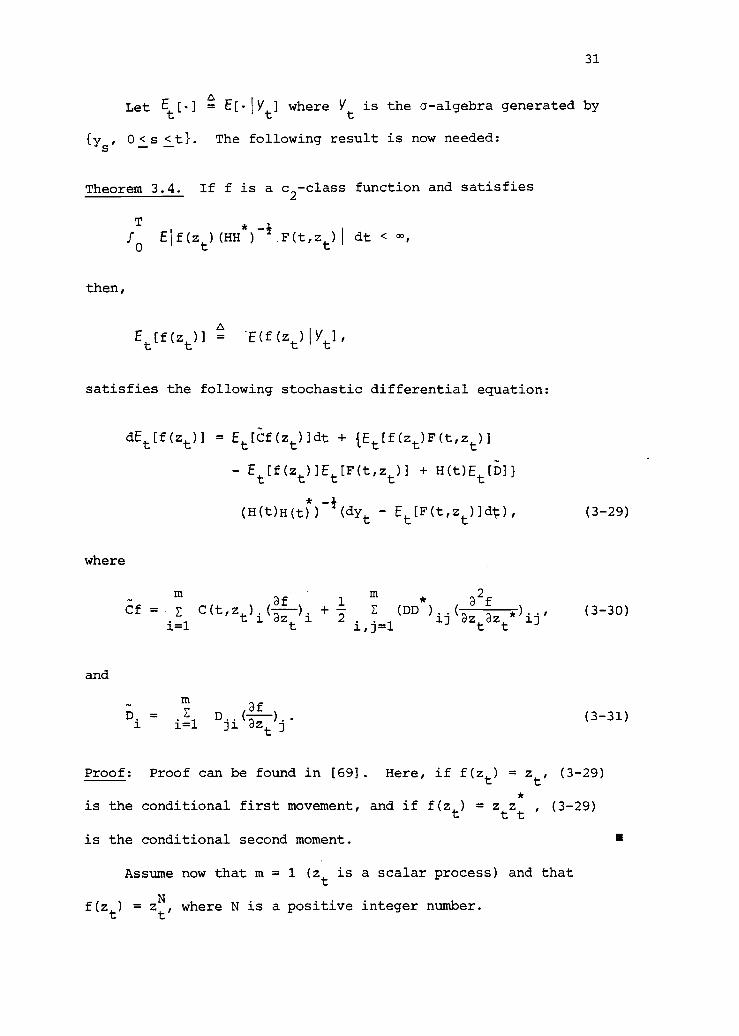
31

Let t[]A

] = EIVt] where V

tis the a-algebra generated by

{17s, 0<s <t}. The following result is now needed:

Theorem 3.4. If f is a c2-class function and satisfies

then,

T *

to Elf(zt)(HH ) F(t,z

t)1 dt < =,

Et(f(z

t)]

A= E(f(z

t)IV

t

satisfies the following stochastic differential equation:

where

and

dEt[f(zt)] = Et[Ef(zt)]cit + tEt[f(zt)F(t,zt)]

- Et[f(z

t t[F(t,z

t)] + H(t)Et[D]}

*(H(t)H(t)) (dY

tEt[F(t,z

t)]#), (3-29)

mCf

D2f

= E C(t,z ) (21-) + 4- E (DD )ij az

taz

t*

)

ij'(3 -30)

i=1t i azt i 2

i,j=1

D. . = D-i=E j1 i

(

az)

tj

(3-31)

Proof: Proof can be found in [69]. Here, if f(zt

) = zt'

(3-29)

is the conditional first movement, and if f(zt) = ztzt , (3-29)

is the conditional second moment.

Assume now that m = 1 (zt

is a scalar process) and that

f(zt

) = zt'

where N is a positive integer number.

a

32

Then, in general, the stochastic differential equation (3-25),

(3-26), (3-27) and performance index (3-28) do not form a closed

system as the equation for dEt[zt

] involves the next higher con-

ditional moment. This means that solution to an infinite di-

mensional set of differential equations may be required in order

to obtain conditional moments of zt

. However, further assumptions

are made here so that either of the following situations occur:

1) The above equations form a finite-dimensional set,

i.e., there exist K > 1 such that for all N > K

E (zt) = function (E (zt), E (z t2),

2), E

t(zt

)); or

2) an approximation technique is used to obtain a finite-

dimensional set of equations for the Kth-conditional

moment of zt.

The information available to the controller allows for a better

mean-square estimate of zt which is given by zt since xt contains

information about ztas well as y

t. Here, it is assumed that

the estimator zt

is suboptimal in the sense that only the obser-

vation ys, s e [0,T], is used to construct the estimate. These

assumptions decouple the control problem and estimation of zt

problem.

In order to solve the suboptimal minimization problem stated

by (3-25) and (3-28), the following approximation of (3-25) is

used:

dxt

At xt dt + u dt + a dwlt t t t,

where

(3-32)

= E[A(t,zt)1Y

t],

Bt = E[B(t,zt) l it] ,

at= E[G(t,z

t)IY

t].

33

(3-33)

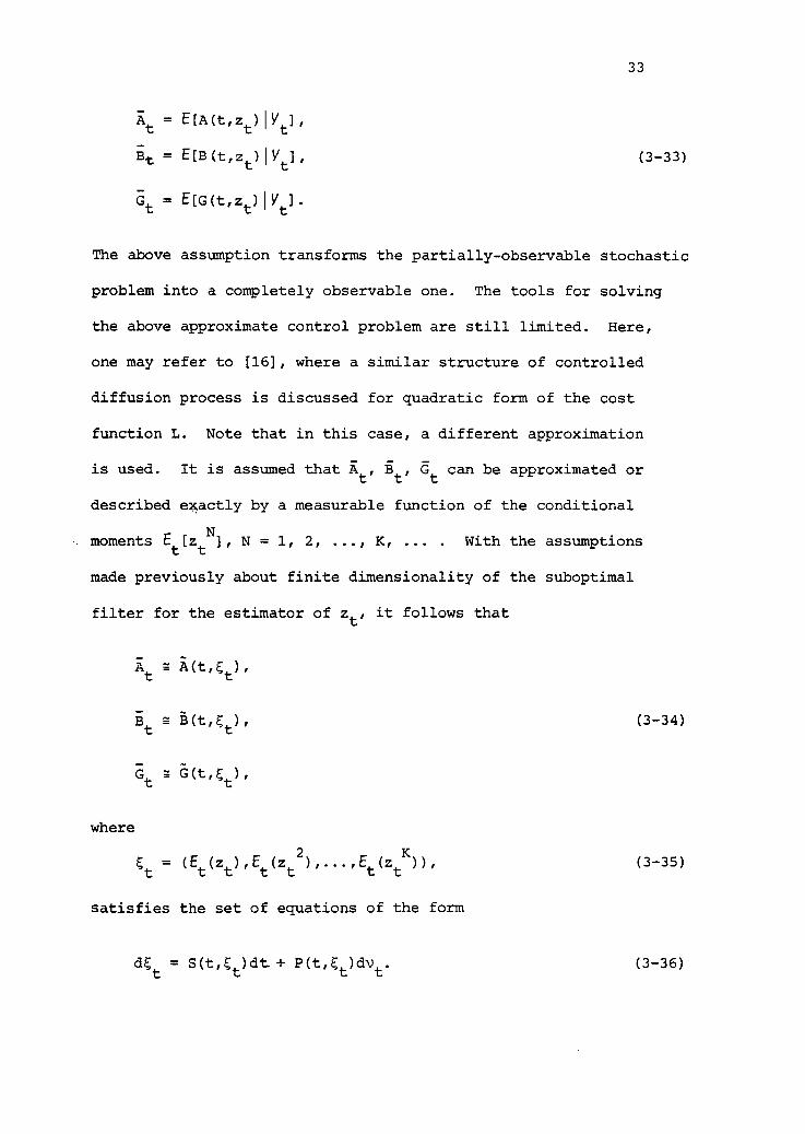
The above assumption transforms the partially-observable stochastic

problem into a completely observable one. The tools for solving

the above approximate control problem are still limited. Here,

one may refer to [16], where a similar structure of controlled

diffusion process is discussed for quadratic form of the cost

function L. Note that in this case, a different approximation

is used. It is assumed that At, Bt, Gt can be approximated or

described exactly by a measurable function of the conditional

moments Et[ztN], N = 1, 2, ..., K, . . With the assumptions

made previously about finite dimensionality of the suboptimal

filter for the estimator of zt

, it follows that

where

_ -

At

A(t,Et),

t t),

at

= a(t,Et ),

Et= (E

t(zt),E

t(zt

2),...,E

t(zt

K)),

satisfies the set of equations of the form

(3-34)

(3-35)

dE = S(t,Et)dt+ P(t,E

t)dy

t(3-36)

34

Now, the approximate, completely observable version of (3-25),

(3-26), (3-27) takes the form of

dxt = ii(t,Et)xtdt + i(t,Et)u

tdt + a(t,E

t)dw

t1,

dEt = S(t,Et)dt + P(t,Et)dvt,

(3-37)

where vtis a Wiener process independent of w

t

1because of the

independence of wt1and wt

2.

If the cost function J(u) in (3-28) is of a quadratic form,

T

J(u) Effo(xtQ(t)x

tutR(t)u

t)dt + xT M xT

The following results apply (29].

Let the following assumptions be satisfied for all t E [0,T],

n E R

1) II i(t,n)I1 + Il B(t,n)II + 11 G(t,n)II < k < co,

where k is a finite positive contant;

2) S(t,n), P(t,n) are such that a unique strong solution

of (3-46) exists andT

Prob. (j"

011 Etll 2dt< co ) = 1;

(3-38)

3) Q(t) and M are non-negative definite, and R(t) is uni-

formly positive definite (i.e., its inverse is uniformly

bounded), and

4) ut

satisfies

I0

E(Ilut2bdt <

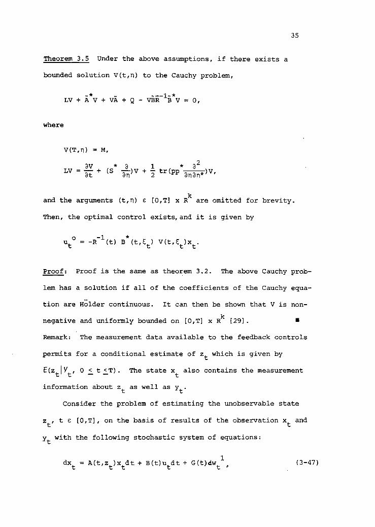
Theorem 3.5 Under the above assumptions, if there exists a

bounded solution V(t,n) to the Cauchy problem,

where

_z- 1-LV + A V + VA + Q - VBR B

*V = 0,

V(T,n) =

at*

an )VLV = + (S -37)V + -2- tr(pp anan*)v,

35

and the arguments (t,n) e [0,T] x Rk

are omitted for brevity.

Then, the optimal control exists, and it is given by

ut

o= -R (t) B

*(t,E

t) V(t,E

t t

Proof: Proof is the same as theorem 3.2. The above Cauchy prob-

lem has a solution if all of the coefficients of the Cauchy equa-

tion are Holder continuous. It can then be shown that V is non-

negative and uniformly bounded on [0,T] x Rk

[29].

Remark: The measurement data available to the feedback controls

permits for a conditional estimate of ztwhich is given by

E(ztIYt

, 0 < t <T). The state x also contains the measurement

information about zt as well as yt.

Consider the problem of estimating the unobservable state

zt, t e [0,T], on the basis of results of the observation xt and

ytwith the following stochastic system of equations:

dxt= A(t,z )x dt + B(t)u

tdt + G(t)dw

t t t

1(3-47)

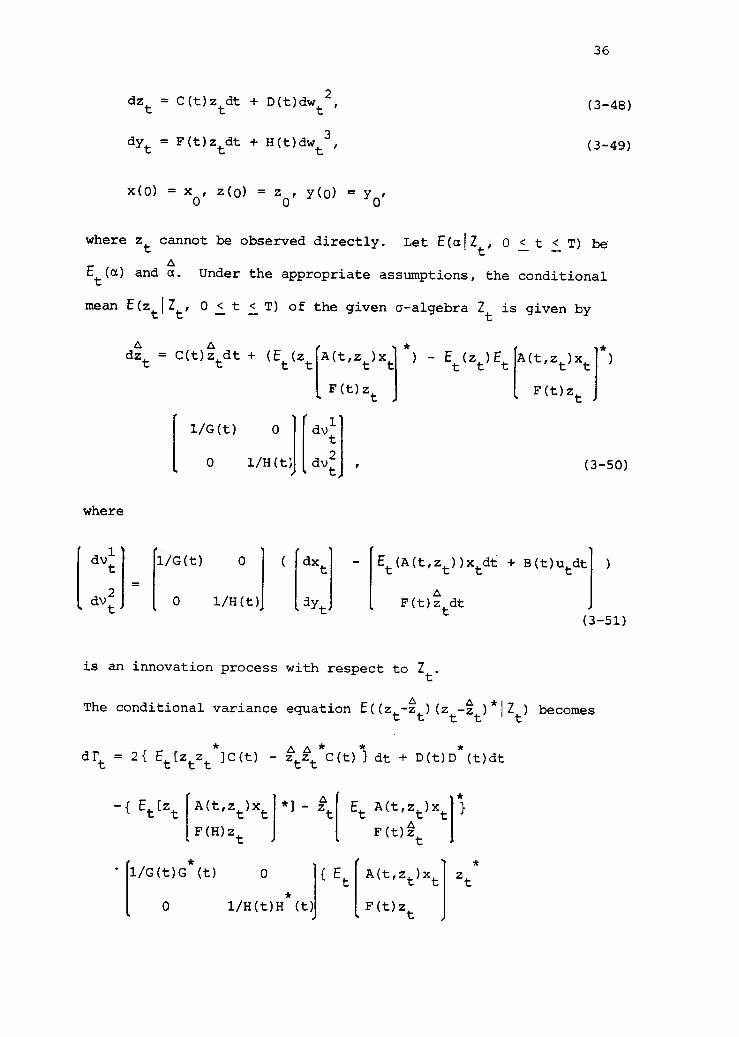
dzt= C(t)z dt + D(t)dw

t

2,

3dyt= F(t)z

tdt + H(t)dw

t '

x(o) = xo

z(0) = zo

Y(0) = Yo

36

(3-48)

(3-49)

where zt cannot be observed directly. Let E(alZt, 0 < t < T) be

Et(a) and a

A. Under the appropriate assumptions, the conditional

mean E(ztlZt, 0 < t < T) of the given a-algebra Zt is given by

a Adz

t= C(t)z

tdt + (E

t(ztA(t,zt)xt ) - E

t(zt)E

t t)xt

*)

F(t)zt

F(t)zt

11/G(t) 0 lid%)

t2

0 1/H(t) dvt

, (3-50)

where

1 /G(t) 0 ( dxt - Et(A(t

'

zt))x

tdt + B(t)utdti )

=

t0 1/H(t) dy

tF (t) Z

A

tdt(3-51)

is an innovation process with respect to Z.

The conditional variance equation E((zt4t)(zt4t)*IZt) becomes

A Aar 2{ E [z

tzt

]C(t) - ztzt*C(t)} dt + D(t)D (t)dt

-{ Et[zt [A(t,zt)xt1 *] - Et

F(H)zt

F(t)zAt

1/G(t)G*(t) 0 { Et

A(t,zt)xt zt

0 1/H(t)H (t) F(t)zt

*

37

fEt A(t,zt)x

tA

A,zt

*Idt + {E

tztzt IA(t,z

t)xtI]

F(t)zt

F(t)zt

Et

[ztzt

] Et A(t,zt)xt

°ztEt[zt* A(t,zt)x

t]

F(t)zt

F(t)zt

A * A A *- z

tEt

[zt

A(t,zt)x

t] + 2 z

tzt

Et(A(t,z

t)x

t}

1/G(t)

[

F(t)z

0

t

dvt

1

F(t)zt

0 1 /H(t) [dvt21 . (3-52)

The conditional mean and variance given observations fx , y ,

s s

s e (0,T]} have infinite dimension in (3-50) and (3-52), respectively.

If there exist E(ztlZt, 0 < t < T) and E((zt-zt)2IZt,

0 < t<T),

the state xtis the solution of the following stochastic equation:

dxt

= Et(A(t,z

t))x

tdt + B(t)u

tdt + G(t)dv

t1

'

(3-53)

where d vt

1is the same as in (3-51). If there exists the con-

Aditional density function p(t,z

t'zt,r

t) corresponding to (3-50) and

(3-52), then, (3-53) may be replaced by the following stochastic

equation,

where

dx = A(t,z ,r )x dt + B(t)u dt + G(t)dvt

1

t ttt (3-54)

A AA(t,zert) = I A(t,zt)p(t,zezert)dzt = E[A(t,zt)IZt]. (3-55)

Consequently the equation (3-54) has been reformulated by ob-

servable processes (3-51) and (3-52).

38

Comment: The conditional estimate E[xtIZ o < t < T] is the

same as xtbecause x

tis Z

tmeasurable.

The innovation process in (3-50) depends on the control vari-

able ut, and thus, the separation principle could not be applied

to verify the optimal control in (3-54). If applied to the sto-

chastic linear controller, this will show that a lower cost can-

not be obtained with nonlinear controls. The optimal control

cannot be found using any well-known methods. For practical

applications the most important results desired are the necessary

conditions of optimality that can be used for synthesis of opti-

mal feedback control laws. The answer to this question is yet

to be resolved.

39

4. SIMULATION OF THE STOCHASTIC CONTROL PROCESSESWITH RANDOM COEFFICIENTS

In previous chapters the problem of optimal control of

stochastic control processes with random coefficients has been

presented. To evaluate the performance of the optimal control

for each stochastic model, it is necessary to synthesize the con-

trol law, the state equation and the solution of a nonlinear par-

tial differential equation. A discretization technique is used

to calculate the state, the Wiener process and the optimal con-

trol for simulation.

A pseudo-Wiener process is used for the generation of the

Wiener process; the first method is introduced by a Bernoulli

time series [70] using pseudo-uniform random numbers between

0 and 1; the second uses pseudo-Gaussian random numbers N (0,1).

The solution of the nonlinear partial differential equation

to the Cauchy problem of equation (2-18) uses a semi-discrete

system of nonlinear ordinary differential equations. The semi-

discrete system equations can be solved by integration of the

ordinary differential equations [71,72,73].

A simple one-dimensional stochastic system has been presented

by the state and optimal control to the value function V(t,xt,zt) =

xt

A1(t,z

t)xt

+ A2(t,z

t). A practical application of the theoretical

extension in Chapters 2 and 3 is presented here by the landing

problem of the longitudinal motion of an aircraft in a gusty wind.

A landing aircraft may be described approximately by a second-

order differential equation with random parameters [44]. Certain

40

information data are derived by conditional estimation using the

given observations. On the basis of observations, the con-

ditional estimate is applied to derive the appropriate sto-

chastic models. This aircraft-landing model is used to illustrate

the design procedure of optimal control under the worst weather

situation. The random parameter is assumed to be the result of

a gusty wind. The models of wind, based on the Dryden model for

turbulence and its aerodynamic effects, are used in conjunction

with optimal-control design.

If the system is subject to both parameter uncertainty and

noise disturbances, control of the dynamic system is treated by

stochastic control theory. The problem of controlling a longitud-

inal motion of an aircraft in wind gust is very similar to the

above problem [34]. The statistical properties of uncertain

quantities, which are Lebesque-measurable functions whose values

may range with proper boundaries, are assumed to be known, and the

stochastic model of longitudinal motion of aircraft in wind gust

is approximated by the second-order stochastic differential equa-

tion. It is also found that the simulation results of the motion

of aircraft in wind gusts give a reasonable degree of approximation.

Using the theoretical results of Chapter 2 and 3, the angle of

attack, the orientation rate of aircraft, the active elevator con-

trol angle, and the active aileron control angle in a gusty wind

are determined.

41

4.1 The Generation of Wiener Process

Let (0,F-,P') be a probability space, Wt, t > 0, be a

Wiener process, and F't be a nondecreasing family of sub-a-algebra

of F'. Then, the Wiener process has the following properties:

i) E(Wt-W

s sIF ) = 0, E((W

t-W

s s)2IF') = t-s, t > s;

ii) Wt2 t

- W and Wt4

- Wt3

are independent for nonover-1

lapping intervals [t2,t

1] and [t4 -t3];

iii) the trajectories Wt

are continuous with probability

1;

iv) w(0) = w0

= 0.

The construction of the Wiener process is most useful to

study the stochastic model. For convenience, the Wiener process

is approximated with the digital computer by a pseudo-Wiener pro-

cess according to the properties of the Wiener process. A contin-

uous stochastic integral for computation can be approximated by

the following discrete Wiener process:

t n-1

og(t)dWt = E g(t.)(W

.

-Wt.

),t

i=0 1+1 1

(4-1)

where g(t) is some suitable function. The discrete representation

of (4-1) should be kept in an infinite sequence of independent

Gaussian variables on Sr.

Consider first, the construction by which a Bernoulli time

series can be made to approximate the Wiener process as follows:

with fixed A > 0, A e [0,T], and the interpolation of certain

random sums,

Wt(A)=h(A)Ez1. , i < t/A, 0 <'t < T,

where z. is the Bernoulli variable which has a mean 0 and a1

magnitude 1. Wt(A) converges to the Wiener process under proper

choiceofthescalarh(A)[53].1f{z.} is a sequence of indepen-

42

(4-2)

dent random variables such that

P[zi=1] = P[zi = -1] =1

(4-3)

and the graph of Wt(A) is a scalar random walk. The scalar h(A)

in (4-2) is selected so that regardless of the value A, the vari-

ance of Wt(A) = t. Thus determine h(A) as follows:

Var[Wt(A)] = t = h(A)

2

i <t/A 1Var[z.],

= [h(A)]2[integer part of (t/A)],

[h(A)]2

A

Therefore h(A) = and Laplace's theorem states

n n -+ co

AT ( I z.) N(0,t).i=1 1

If n is t/A, then h(A) = 1/.711. and letting A .4- 0,

n n

Wt(A) = h(A) E z1. = E. . 11=1 1=1

(4-4)

(4-5)

(4-6)

Since z. are independent, for t1 < t2< ...< to = T, W

tl

, Wt

- wt

,

2 1

Wt

- Wt

are statistically independent and the stochasticn n-1

43

process Wt(A) converges, as A 0, to the Wiener process W.

If there exist independent uniform random variables ri,r2...,

rnxm

between

z.1

=S

0 and 1, define the following random variables as

1

0 < r. < 0.51

t-1 0.5 < ri < 1.0, i = 1,2,..., n x m.

Hence, p(xi=1) and p(xi=-1) are 1/2. The approximate Wiener

process is given by

1

(4-7)ti nxmW=---2(Ez.), j = 1,2,...,m, i = 1,2,...,n x m,t. man 1

3 i=1

wherenxm=t./A is total number of random variables z.1between

t.and0,andAisthesmalltimeintervalt.-ti-l. Equation

(4-7) is equivalent to

n(m-1)W = 1 / 2 7 ( E z

1) . * W

t.J i=1 3-1

(4-8)

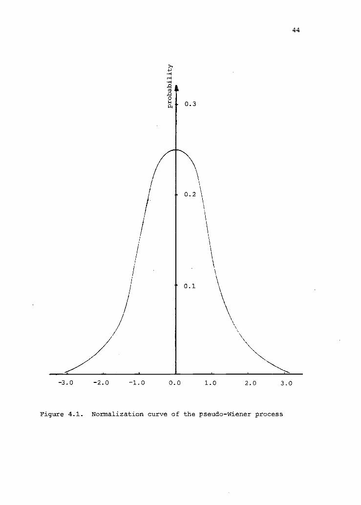
Figure 4.1 shows the normalization curve of (4-8) for t 6 [0,1],

o = 0.001, n = 1000, m = 10. 10,000 total uniform pseudo-random

variables are used to generate 1,000 discrete Wiener processes.

Let W. be a normal random sequence. In this case, (Wt.

- Wt

has the mean 0 and variance ). Hence, the standard

Brownian motion is always calculated by simply taking the linear

function oft t.

has the distribu-. , 33 3-1 3

tj-1

tion N(0,t.-t. )), W" = W /(t.-t. ) has the distribution N(0,1).J J-1

W. /(t. -t.3 3-1

Table 4-1 shows the distribution of lAr for 1000 normal random vari-J

ables in the range of -3.5 < < 3.5 with the distribution of loIr

being

44

-3. 0 -2.0 -1.0 0.0 1.0 2.0 3.0

Figure 4.1. Normalization curve of the pseudo-Wiener process

45

TABLE 4.1 THE DISTRIBUTION OF THE NORMALIZED PSEUDO-WIENERPROCESS FOR 1000 RANDOM NUMBERS

Range Numbers Probability of Each Range

- 3.5 < W: < -3.0

-3.0 < W: < -2.5

- 2.5 < W. < -2.0

- 2.0 < < -1.5

- 1.5 < W. < -1.0

- 1.0 < W: < -0.5J

- 0.5 < W: < 0

W:= 0J

0.0 < W. < 0.5

0.5 < W. < 1.0

1.0 < W: < 1.5

1.5 < W. < 2.0

2.0 < W: < 2.5

2.5 < W: < 3.0

3.0 < W: < 3.53

1

10

0

41

102

204

0

251

0

217

126

37

0

10

1

0.001

0.010

0.000

0.041

0.102

0.204

0.000

0.251

0.000

0.217

0.126

0.037

0.000

0.010

0.001

46

P( -3 < < 3) = 0.998 :4 1.0.

As illustrated by Figure 4.1 the density and the results of Table 4.1,

it is a good approximation for 1000 discrete Wiener process.

These random variables are checked for the student t-distri-

bution which (n-1) degree of freedom. The normalized Wiener

increments IC: in Table 4.2 is given by the t-test. All t values

in Table 4.2 are less than the critical values, and therefore,

the results satisfy the t-distribution. Hence, the pseudo-Wiener

process is assumed to be equivalent to the Wiener process.

TABLE 4.2 THE RESULTS OF THE STUDENT t-DISTRIBUTION

Numbers of NormalRandom Variables Used Critical Values The Given t Value

100 3.389 1.3493

200 3.389 1.5315

500 3.310 1.7067

1,000 3.291 1.8862

Apply the above Wiener-process simulation results to the sim-

ple first-order stochastic system

dxt = A(t)xtdt + G(t)dW , (4-9)

where the mean mtand variance S

tof x

tare

mt

= A(t)mt

m(0) = m0

St

= 2A(t)St

+ G(t)2

, S(0) = S.

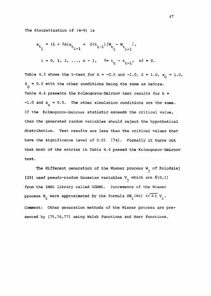
47

The discretization of (4-9) is

. 101

Wt ]'.

+ G[txt

= (1 + 6A)xt 1-1

)(t, .

1-1

i = 0, 1, 2, ..., n - 1, (5= tt

- tt-1

, n6 = T.

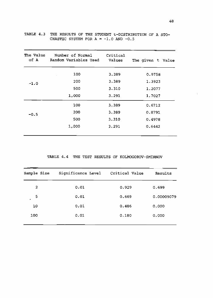
Table 4.3 shows the t-test for A = -0.5 and -1.0, G = 1.0, x0

= 1.0,

S0= 0.0 with the other conditions being the same as before.

Table 4.4 presents the Kolmogorou-Smirnov test results for A =

-1.0 and xo

= 0.5. The other simulation conditions are the same.

If the Kolmogorov-Smirnov statistic exceeds the critical value,

then the generated random variables should reject the hypothetical

distribution. Test results are less than the critical values that

have the significance level of 0.01 [74]. Formally it turns out

that most of the entries in Table 4.4 passed the Kolmogorov-Smirnov

test.

The different generation of the Wiener process W. of Kolodziej

[29] 11secipseudo-randorriGaussiarivariablesNLwhich are N(0,1)

from the IMSL library called GGNML. Increments of the Wiener

process Wtwere approximated by the formula dW.(At) -( Vi.

Comment: Other generation methods of the Wiener process are pre-

sented by [75,76,77] using Walsh functions and Harr functions.

48

TABLE 4.3 THE RESULTS OF THE STUDENT t-DISTRIBUTION OF A STO-CHASTIC SYSTEM FOR A = -1.0 AND -0.5

The Valueof A

Number of NormalRandom Variables Used

CriticalValues The given t Value

100 3.389 0.9758

-1.0200 3.389 1.3923

500 3.310 1.2077

1,000 3.291 1.7027

100 3.389 0.6712

-0.5200 3.389 0.8791

500 3.310 0.4978

1,000 3.291 0.6442

TABLE 4.4 THE TEST RESULTS OF KOLMOGOROV-SMIRNOV

Sample Size Significance Level Critical Value Results

2 0.01 0.929 0.699

5 0.01 0.669 0.00009079

10 0.01 0.486 0.000

100 0.01 0.180 0.000

49

4.2 Numerical Solutions of NonlinearPartial Differential Equations

The problem of solving (2-13) for given Al(T,zT), and

A2(T,z

T) is called the Cauchy problem. The solution is understood

to be continuous in Rnx [0,T] and to have continuous derivatives

aA1

DA2

3A1

ant a2A1

a2A2 n

atI

atI in R x [0,T]. The solutionI

aE,

to problems in (2-13) may be transformed to initial-boundary value

problems for t replaced by T-s, t,s e [0,T]. Then, (2-13) becomes

the classical Cauchy problem with the initial conditions instead

of the terminal conditions.

Let

ank DA

1aA

2aANP

atfk (t,E,A1,A2,...,ANp, , , ,

a2A1 a2A2a2 ANP

aEaE*' aEaE*' aEaE*" (4-10)

k = 1, 2, ..., NP,

denote the coupled systems of partial differential equations with

the initial conditions

(4-11)A1

1

s=0= k

1, A

21

s=0= k

2, . . , A

NP1

s=0= k

NP,

where k. is some constant. Kolodziej [29] proved that the partial

differential equation (4-10) with (4-11) has a bounded unique solu-

tion.

The numerical solution of the nonlinear partial differential

equation is complicated and is a highly problem-dependent process.

The semi-discrete system of nonlinear ordinary differential

50

equations is solved using one of the recently developed ordinary

differential equations integrator [71,72]. The numerical method

of lines [42] will be used for equation (4-10). Describe the

finite difference approximations used by the computer simulation.

Assume that a user has specified a time-independent spatial mesh

which consists of a sequence of NS(?3) points in [a,b] such that

= b. Define the mesh spacing as A. =a El < E2 < ...< ENS

g1

-i +1

E., for i = 1,2,...,NS-1. Associate with this mesh the1

functions A. .(s), j = 1,2,...,NP where j is the number of the3,1

partial differential equations, and i = 1,2,...,NS. The value

of the function A. (t) at any time t is meant to approximate

the true solution value A.(s, .). To obtain an ordinary differ-E3

entialequationwhichwilldetermineA..(s), evaluate the jth3,1

partial differential equation (4-10) at E=Ei where 1 < i < NS.

For numerical solution, evaluation of A, AE, and

an7 N

9 E,, j= 1,2, ... , NP,

is necessary. Let the approximations A. . (s) denote A. ..7,1 7,1

For E=E. in the jth partial differential equation, approximate1

A.(s,E) 1' A..,J 31

3A.(s,) A. -A. .

, 3(1+1) 3 (1-1)

3E A Aj i-1

3A.3 (s,E) 1 (4-12)=

3E( )

3E(Ci+14-Ei)/2 (Ei-14-Ei" 2

(

A A.. A..

Aj(1+1) 31

31 3(i-1)), j=1,2,..., NP.1 i-1

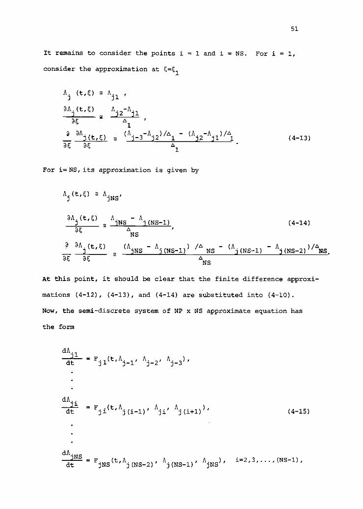
51

It remains to consider the points i = 1 and i = NS. For i = 1,

consider the approximation at E=E1

A. (t,E) ,1 A.1

an. t,E) A Aj2 jl

aE of '

a an. (Aj-3Aj2)/A1 (Ai2-Ail)/Li

aE aE of

For i= NS, its approximation is given by

A.(t,E) AjNS

,

(4-13)

an_ (t,E) A. - A3 DNS j(NS-1) (4-14)aE A ,

NS

a aA . - A.iet,E) (A - A

jNS 3(NS-1)) /6,

NS ( Aj(NS-1) 3(NS-2)) / ANS.

aE 3E aNS

At this point, it should be clear that the finite difference approxi-

mations (4-12), (4-13), and (4-14) are substituted into (4-10).

Now, the semi-discrete system of NP x NS approximate equation has

the form

dA.

=F. (t,A A. , A),dt jl j-1' 3-2 . j -3

dA.,

-IL F..(t,A A. , A. ),dt 31 j(i-1)' 3i 3(i+1)

dA.

iNS F.dt 3NS 7

AA (NS-2) 3 (NS-1)

AjNS ),

(4-15)

i=2,3,..., (NS-1),

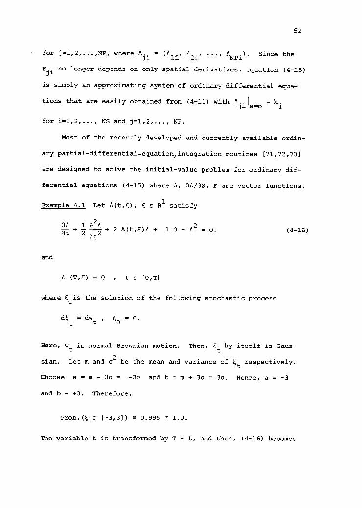
52

for j=1,2,...,NP, where A.. = (A, A2i, ..., A ). Since the31 NPi

F.. no longer depends on only spatial derivatives, equation (4-15)31

is simply an approximating system of ordinary differential equa-

tions that are easily obtained from (4-11) with A..' = k.31 s=o

for i=1,2,..., NS and j=1,2,..., NP.

Most of the recently developed and currently available ordin-

ary partial - differential - equation, integration routines [71,72,73]

are designed to solve the initial-value problem for ordinary dif-

ferential equations (4-15) where A, 3A/9S, F are vector functions.

Example 4.1 Let A(t,E), E e R1satisfy

and

3A 1 3 A2

+ + 2 A(t,E)A + 1.0 - A2 = 0,aE

A (T,E) = 0 , t e [0,T]

where Et is the solution of the following stochastic process

dEt = dwt

, E0

= 0.

(4-16)

Here, wt

is normal Brownian motion. Then, Etby itself is Gaus-

sian. Let m and a2 be the mean and variance of Et

respectively.

Choose a = m 3a = -3a and b = m + 3a = 3a. Hence, a = -3

and b = +3. Therefore,

Prob.(E e [-3,3]) '=" 0.995 z 1.0.

The variable t is transformed by T - t, and then, (4-16) becomes

Let

2A- + 2A(t,E)A - 1.0 + A2.

= 0.1, i = 1,2,..., 61,

At

= 0.001, t c [0,1],

rA = Ao + Al tan

-1(c),

53

Ao

= 3.75,

Al = 1.50.

Figure 4.2 shows the numerical solution of (4-16) for the five

different values: a) Ao= 3.75, and Al = 1.50, b) A

o= 3.2, and

Al = 1.2, c) Ao = 2.5, and Al = 1.0, d) Ao = 2.0, and Al = 0.75,

e) Ao= 1.5, and Al = 0.5. The solution A is similar to the

following Riccati equation:

9A'- 2A0A"- 1.0 +A-2.

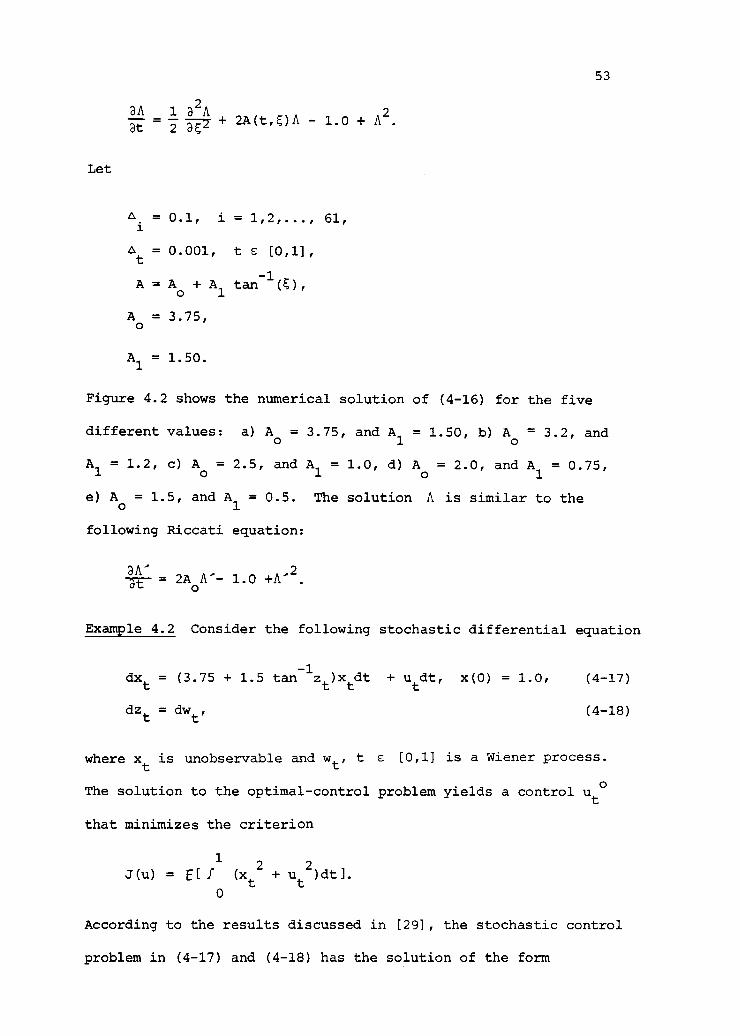
Example 4.2 Consider the following stochastic differential equation

dxt= (3.75 + 1.5 tan

-1zt)x

tdt + u dt, x(0) = 1.0, (4-17)

dzt = dwt, (4-18)

where xt is unobservable and wt, t e [0,1] is a Wiener process.

The solution to the optimal-control problem yields a control ut°

that minimizes the criterion

1

J(u) = (xt

2+ u

2)dt].

0

According to the results discussed in [29], the stochastic control

problem in (4-17) and (4-18) has the solution of the form

a)

SI.4)

0.2

0.4

0.6

0.8

1.0

54

Figure 4.2 Solutions of the Riccati equation for (a) Ao = 3.75,

(b) Ao = 3.2, Al = 1.20, (c) Ao = 2.5, Al = 1.0,

(d) Ao= 2.0, Al = 0.75, (e) A

o= 1.5, Al = 0.5

where

55

ut

o= - V(t,z

t)mt

,

dmt = (3.75 + 1.5 tan-lzt

V(t,zt));

tdt, m

0= x0,

and V(t,E), E e R satisfies

32

at1 V

+ -37 + 2-(3.75 + 1.5 tan-lzt)V + 1.0 - V2 = 0,

V(1,E) = 0, t e [0,1].

Using the simulation results in example 4.2, Figure 4.3 shows that

optimal control and suboptimal control obtained for (4.17) with

(3.75 + 1.5 tan1zt

) replaced by E[3.75 + 1.5 tan-1

zt]. Figure 4.4

shows the sample paths according to optimal control and suboptimal

control in (4-17).

4.3 Application to an Aircraft Landing Problem

Landing aircraft may be described approximately by a second-

order differential equation with random coefficients [44].

d2h(t)

= r(a, v, dl, 62

, s3. d4, 65)u

t,

dt2

(4-19)

where h(t) is the altitude; ut

is the altitude control signal;

r is a coefficient depending on air density a, the flight velocity

v, and aerodynamic coefficients 81, 82, 83, 84, 85. At the begin-

ning of the landing process, the initial conditions are given by

h(0) and h(0). The flight velocity v is assumed to be constant

throughout the landing process with finite inverval of landing

time T. The coefficient r, which characterizes the objective of

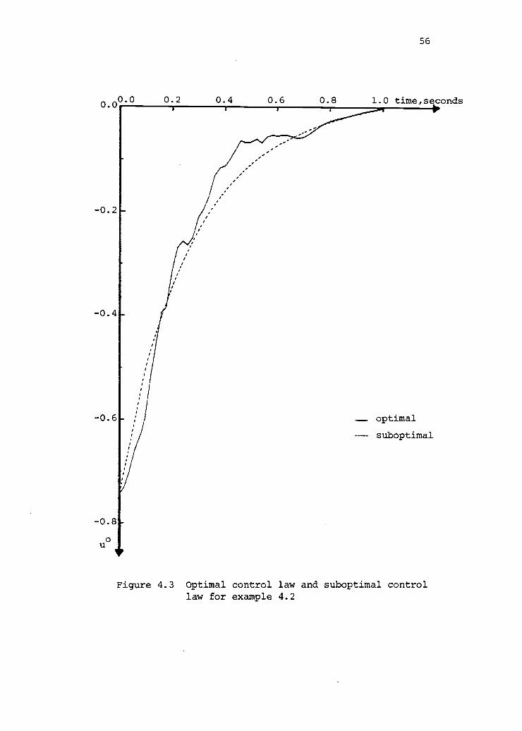
56

0.2 0.4 0.6 0.8 1.0 time,seconds

optimal

-- suboptimal

Figure 4.3 Optimal control law and suboptimal controllaw for example 4.2

FOR OPTXMAL

tFOR SUBOPTZMAL

exeRaLizationampie 4.2

of xt under optima/ and for

57

58

control, depends on many factors that can vary randomly at any

moment in time. If the altitude has an additive noise process,

then (4-19) may be modified as follows:

2d h(t)TOT = r(t,zt)ut + Nt, (4-20)

where Nt is a white noise process. Letting the state variable

xtrepresent the descent rate h(t), the stochastic model in the

sense of Ito differential form may be described by

dxt= r(t,z

t)u

tdt + g(t)dw

t

1, x(0) = x0, xt R1. (4-21)

the equation (4-21) is meaningful insofar as it's an integral equation

[55]. It is assumed here that the random parameter r is dependent

on a certain unobservable stochastic process,

dzt = C(t,zt)dt + D(t)dwt

2, z(0) = z0, zt a R1,

and yt is an observable process satisfying

dyt= F(t,z

t)dt + H(t)dw

t

3.

Here wtl , wt2 , wt3 are mutually independent Wiener processes.

The cost fuction, which depends on the rate of descent of the

aircraft during the landing interval and the control system ut, is

given in the quadratic form

J(u) = E[0

ut2dt + Mx T2]. (4-22)

The above control system has the structure discussed in Chapter 3,

and the corresponding results can be applied here. Assuming that

59

the first two conditional moments of ztsatisfactorily estimate

zt, the following approximation of (4-20) can be used:

dxt= r(t,z

t,rt)utdt + g(t)dw

t

1,

-

t

21where zt

is E[ztlyt

] and rt

= E[(zt-z ) 1 Y ).

t

One of the possible models for the wind gust velocity is

suggested by Balakrishnan [11,42] such that

(4-23)

t= - az

t+ an

t, a > 0, a > 0, (4-24)

and ntis a white Gaussian noise with unit spectral density.

Hence ztis Gaussian, asymptotically stationary, with the spectral

density function given by

P(w) -2

472w2+a

2(4-25)

where P(w) is called the spectral distribution of zt

. Equation

(4-24) has its stochastic differential form as

dzt

= -aztdt + adw

t

2,

and the observation process is assumed to be of the form

dyt

= fztdt + dw

t

3.

(4-26)

(4-27)

Here wtl, wt2, wt3 are assumed to be mutually independent Wiener

processes. Now the suboptimal filter for ztreduces to the Kalman

filter, and the conditional density with respect to Yt is Gaussian.

It follows that

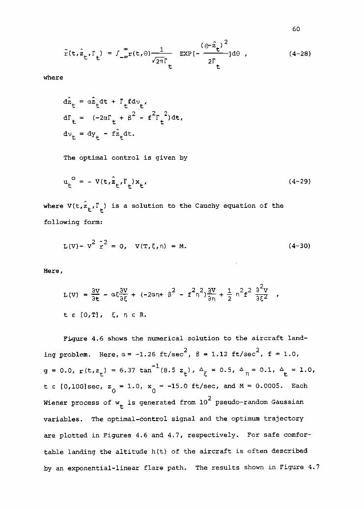
where

1

)2

r(t,zt,Ft

) = 1 EXP[-...r(t,O) ]d0 ,

/Tr-Ft

2rt

dzt

= aztdt + r

tfdv

t,

drt

= ( -tart + 82 - f2rt2 )dt,

dut

= dyt

- fztdt.

The optimal control is given by

ut

o= - V(t,z ,r

t)xt

,

where V(t,zt,rt

) is a solution to the Cauchy equation of the

following form:

Here,

-L(V)- V

2r2

= 0, V(T,,n) = M.

3V ,2 2 2 3V 1 2 2 32V

L(V) = - + (-2an+o-fn) +3t DE n 2

t e [0,T], E, n E R.

60

(4-28)

(4-29)

(4-30)

Figure 4.6 shows the numerical solution to the aircraft land-

ing problem. Here, a = -1.26 ft/sec2

, S = 1.12 ft/sec2

, f = 1.0,

g = 0.0, r(t,zt

) = 6.37 tan-1

(8.5 zt), A

E= 0.5, A = 0.1, A

t= 1.0,

t e [0,100)sec, z0= 1.0, x

0= -15.0 ft/sec, and M = 0.0005. Each

Wiener process of wt

is generated from 102pseudo-random Gaussian

variables. The optimal-control signal and the optimum trajectory

are plotted in Figures 4.6 and 4.7, respectively. For safe comfor-

table landing the altitude h(t) of the aircraft is often described

by an exponential-linear flare path. The results shown in Figure 4.7

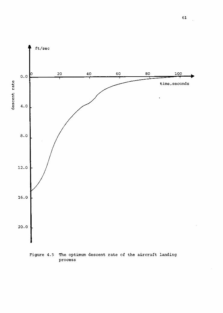
0.0

4.0

8.0

12.0

16.0

20.0

ft/sec

0 20 40 60 80 100

61

time, seconds

Figure 4.5 The optimum descent rate of the aircraft landingprocess

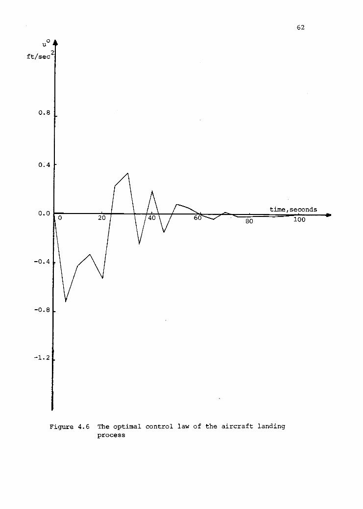
62

time,seconds40 60

80

Figure 4.6 The optimal control law of the aircraft landingprocess

100

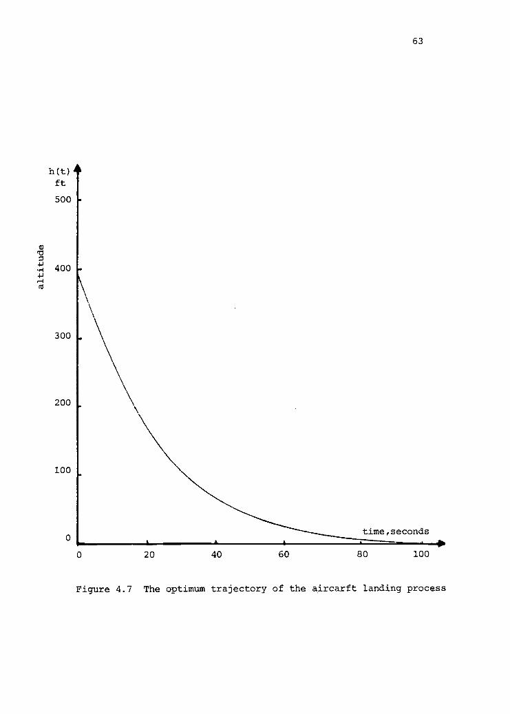
h(t)

ft

500

ro

400

300

200

100

0

63

time,seconds

0 20 40 60 80 100

Figure 4.7 The optimum trajectory of the aircarft landing process

64

is almost the same as the expoential-linear flare path so popular

in landing systems.

4.4 The Control Problem of LongitudinalMotion of an Aircraft in Wind Gust

The control of dynamical systems which contain uncertain ele-

ments and are subject to uncertain inputs may be treated by sto-

chastic control theory. Leitmann [32,33] presented studies of un-

certain dynamical systems which have an unstable mode, and he treat-

ed the estimated state-feedback control to assure ultimate bounded-

ness of given states for a Lyapunov function. The purpose of this

section is to develop systematic techniques for the design of an

optimal-control law which will minimize the effect of the wind

disturbances and noises to an aircraft in a gusty wind. The con-

trol of dynamical systems which include unknown parameters and are

dependent on uncertain quantities are estimated by an appropriate

filtering algorithm. Even with a stochastic model of the wind gusts,

there still remains the nontrivial work of computing the statistical

response of an aircraft flying through such a wind-gust field. In

virtually all analyses of aircraft wind-gust response, which this

author has found, the incremental aerodynamic force at each point

on the aircraft are assumed to depend lineraly upon the wind-gust

velocity. While such assumption may be somewhat questionable in

general, its use in the Dryden model for turbulence yields a reason-

ably accurate description of the wind gust effects.

Consider the control problem of longitudinal motion of an

aircraft in wind gust [34]. Let

x1= angle of attack

= orientation of aircraft

x2= 0

u1= active elevator - control angle

u2= active aileron control angle

wt= Wiener process

For such system, a stochastic dynamic equation of the motion of

the aircraft is given by

dxt = A(t,zt)xtdt + B(t,zt)utdt + G(t)dwt,

x(0) = x0, xte R2

,

where A(t,zt

) and B(t,zt

) are uncertain parameters, and wtmodels

the fact that the angle of attack xl and orientation of aircraft

0 are difficult to measure. Let the presence of the stochastic

process ztmodel wind gust, where z

tsatisfies

dzt = C(t)ztdt + D(t)dwt1

, z(0) = z0, Zt E R1

65

(4-31)

with observation

dyt

= F(t)ztdt + H(t)dw

t

2, y(0) = 0, yt e R1 ,

(4-32)

(4-33)

where C(t), p(t), F(t), H(t) have appropriate dimensions and wt,

wt1, wt

2are independent Wiener processes.

An approximate description of (4-31) may be given by the

following stochastic differential equation:

dxt

1.= A(t,zt, yt)xtdt + B(t,zt,Yt)utdt + G(t)dw

t, (4-34)

where xt= [x

1,x

21, u

t= [u1,u2], and z is E[z

tIYt

] and y is

!

-

E[(zt-z

t*

)21Yt]. Here, A(t,z

t,y

t), and B(t,z

t,y

t) are given by

66

i(t,;t t

) = I -oA.(t 'E) 1 EXP (E-;t)2Yt-1)dE

iT7t-

co, ,

B(t,zt,y

t) =I

-co

1B(t,E) EXP

1

t)

2Yt

-1,. (4-35)

12-717-t-

The conditional expectation ztand the conditional covariance y

t

are given by the following equations:

di = C(t)i dt + ytF(t)(H(t)

2) (ay

tF(t)z

tdt),

dyt

= (D(t)2

- y(t)2F(t)

2(H(t)

2)

-1+ 2C(t)yt)dt, (4-36)

zo= E(z

0) , y

0= Cov(z

o).

If the state xt

= [x1,x

2] is observable, the minimization

of the following cost function J(u) can be made:

*J(u) = tp (xt

Qxt+ u

t

*Ru

t]dt .

Then the optimal control ut° satisfies

(4-37)

-*ut

-1B(t,ztt= -R ) (A

1(t,z

t,yt)xt

1+ A

2(t,z

t,Yt)), (4-38)

2

where A1(t,z

t,y

t) and A

2(t,z

t,yt

) are solutions to the following

nonlinear partial differential equations:

111 = -A*A1

- A1A + Q A

1BRleA

1- (FE) -2-

Al

1 2 2 a2

- -2- (T1 F -5-a-e1) - (D2-n F

2(H

2)

-1 + 2Cn)a A1,

-1* 1 . 2_2

3E2A2= -A

2i - A

2BR B A

1- (FE)

aEA1 2

- 01 F ----3E

A2

)

(D22 2 2

- (D - n F (H )

-1)A .an 2

Here, the arguments (t,E,n) are omitted for brevity, and

(4-39)

67

A1(T,E,T1) = 0, A

2(T,E,n) = 0, E E R1, n e R

1.

For the case when the state xt = [x1,x

2] is unobservable,

the control problem has been solved for a linear system with quad-

ratic criterion having random coefficients [29]. Consider the

following observation equations:

= 0 xl dt + 0 dwt2

dy2 0 a2

x2

0 e2

dwt3

'

(4-40)

where wt2

and wt3

, t e [0,T], are Wiener processes and are independent

of

P[

t e

where

wt and

Let

xi(o)

x (0)

[0,T],

dmt

drt

dvt

m0

r0

vt

wt

1)

=

=

=

=

is

1

to

<

are

i(t,;

(Ar

dy

E[x

E [(x

a

,

kl

k2

t

2

0

Wiener

respectively.

3)

2

unique,

t,Y

+

1[Y

-m0

in

r

a

Y

0

Chapter

y1(o)

y2 (o)

continuous,

t) m

tdt

*

tA +

2m2dt

1(0)1

2(0)

(x -m0

process,

]is

+

GG

,

]

) I

0

2 be satisfied

p-a.s. Gaussian.

Yt-measurable

t,y

t

*- r a (cc

y1(0)1 )

y2(0)

and a =

tdt +

*) art

al 0

0 a2

and also

Then

solutions

r a*(ee*)-1d

)dt,

, e =

assume

mt

and

v

el 0

0 e2

that

rt

,

to

,

(4-41)

.

68

Here, the equation (4-41) stems from the equations (4-34) and

(4-40).

There is a parameter of particular significance to aircraft

and missiles, namely the angle of attack defined by the following

relation:

a = tan-1 (

w),

where w and uare velocities of X and Z directions, respectively.

This is the angle between the relative wind and the longitudinal

axis resolved into the XZ-plane. A frequently accepted alteration

facilitating the mathematics is the approximation of constant

forward speed. Certainly aircraft are capable of flight over a

very wide speed range but the dynamic motions that are most de-

sirable for analysis occur in a relatively short period of time

on the order of a few seconds - during which no appreciable speed

change takes place. In face axial accelerations of the order of

which aircraft are usually subjected do not significantly affect

their dynamic motion. Under this assumption, the angle of attack

is

-1a = tan (

constant)

Aerodynamic forces and moments are strictly speaking functions of

certain state variables. Consider for example variable angle of

attack a(t), -7 < a(t)< 1r, on wing with velocity w(t) and u(t).

Using aerodynamic derivatives or stability derivates [78] with re-

spect to the longitudinal-motion variables, expressions of

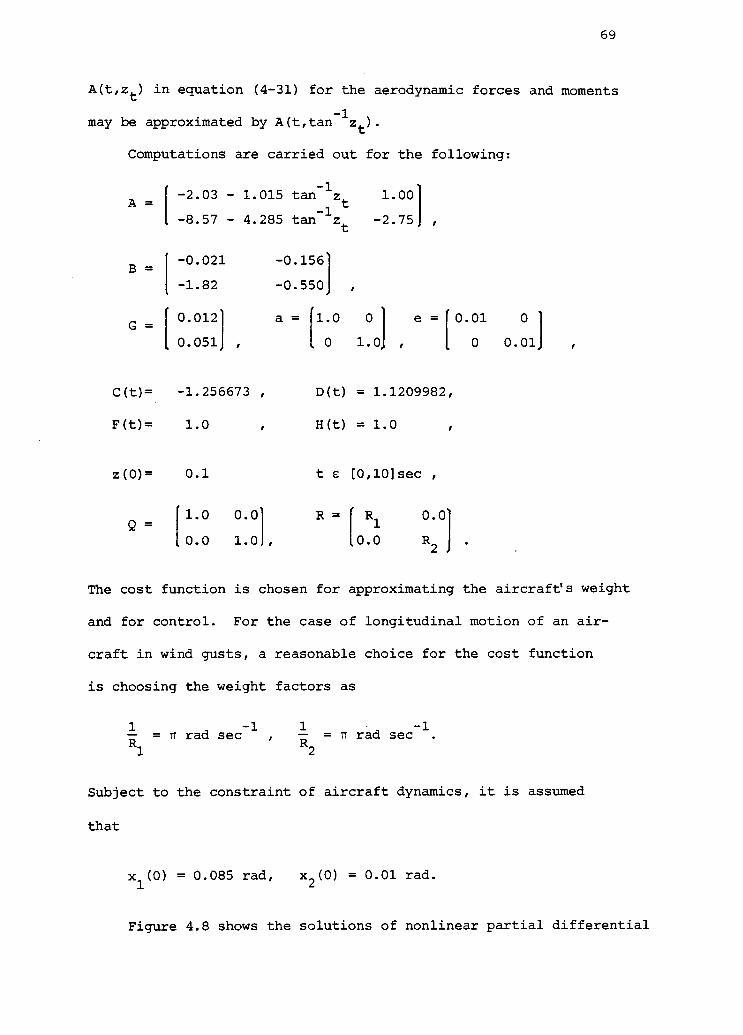
69

A(t,zt) in equation (4-31) for the aerodynamic forces and moments

,

may be approximated by A(t,tan-1

zt).

Computations are carried out for the following:

B =

1-2.03 - 1.015 tan-1

-8.57 - 4.285 tan-1

-0.021 -0.156

-1.82 -0.550

zt

zt

G =0.012 a = [1.0

0.051 , 0

C(t)= -1.256673 , D(t)

F(t)= 1.0 H(t)

z(0)= 0.1 t e

1.0 0.0 R =Q =

0.0 1.01,

1.00

-2.75 ,

0 I e =[ 0.01 0

1.0 , 0 0.01] ,

= 1.1209982,

= 1.0

[0,10]sec ,

Ri 0.0

I .0.0 R2

The cost function is chosen for approximating the aircraft's weight

and for control. For the case of longitudinal motion of an air-

craft in wind gusts, a reasonable choice for the cost function

is choosing the weight factors as

1 = Tr rad sec-11R = Tr rad sec-1.

R12

Subject to the constraint of aircraft dynamics, it is assumed

that

x1(0) = 0.085 rad, x

2(0) = 0.01 rad.

Figure 4.8 shows the solutions of nonlinear partial differential

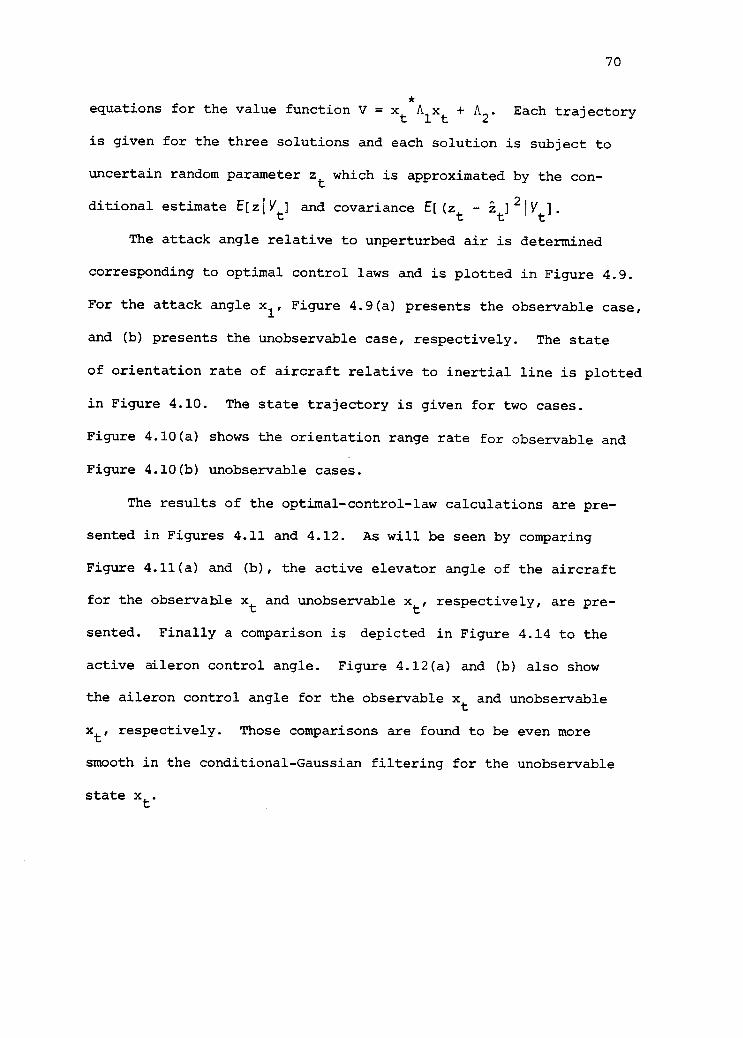
70

equations for the value function V = xt Alxt + A2. Each trajectory

is given for the three solutions and each solution is subject to

uncertain random parameter zt which is approximated by the con-

ditional estimate E[zIYt

] and covariance El(zt

- zt

]

21Yt1.

The attack angle relative to unperturbed air is determined

corresponding to optimal control laws and is plotted in Figure 4.9.

For the attack angle x1,

Figure 4.9(a) presents the observable case,

and (b) presents the unobservable case, respectively. The state

of orientation rate of aircraft relative to inertial line is plotted

in Figure 4.10. The state trajectory is given for two cases.

Figure 4.10(a) shows the orientation range rate for observable and

Figure 4.10(b) unobservable cases.

The results of the optimal-control-law calculations are pre-

sented in Figures 4.11 and 4.12. As will be seen by comparing

Figure 4.11(a) and (b), the active elevator angle of the aircraft

for the observable xt and unobservable xt, respectively, are pre-

sented. Finally a comparison is depicted in Figure 4.14 to the

active aileron control angle. Figure 4.12(a) and (b) also show

the aileron control angle for the observable xt

and unobservable

xt, respectively. Those comparisons are found to be even more

smooth in the conditional-Gaussian filtering for the unobservable

state xt.

A ,A11 22'

A12 0.8

0.6

A11

st,

0.4

0.2A22

Pr

5.0It 10.00.0

Itime,seconds

A-0.2 12

-0.4

0.6

Figure 4.8 Solutions of Riccati-like-equation for the control oflongitudinal motion of an aircraft

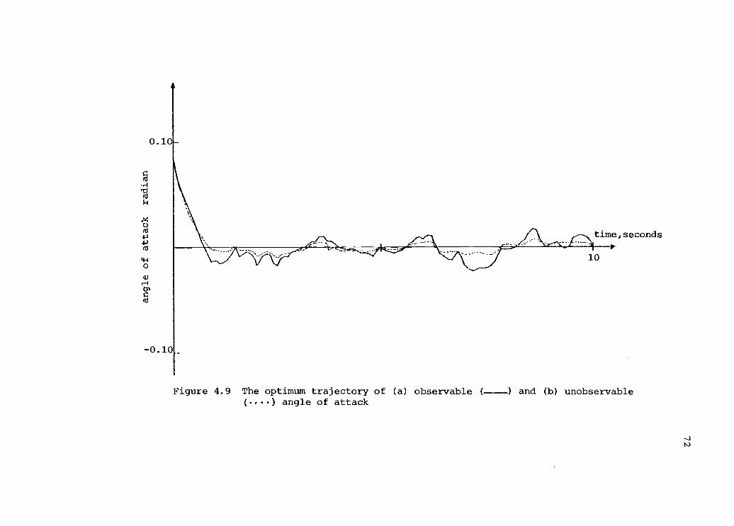
time, seconds

10

Figure 4.9 The optimum trajectory of (a) observable ( ) and (b) unobservable(.) angle of attack

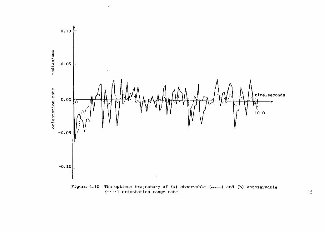
0.10

0.05

0.00

0.05

- 0.10

time,seconds

Figure 4.10 The optimum trajectory of (a) observable ( ) and (b) unobservable() orientation range rate

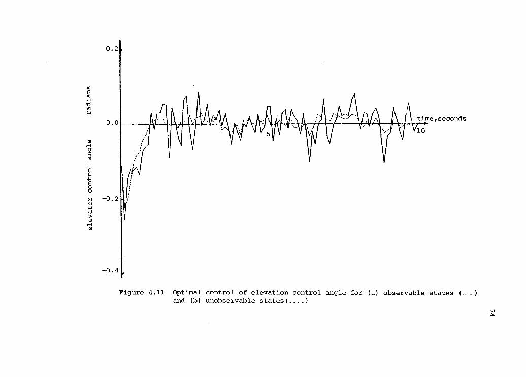
U)

r1

0.2

0.0

0.2

0.4

1\

time, seconds

V10

Figure 4.11 Optimal control of elevation control angle for (a) observable statesand (b) unobservable states(....)

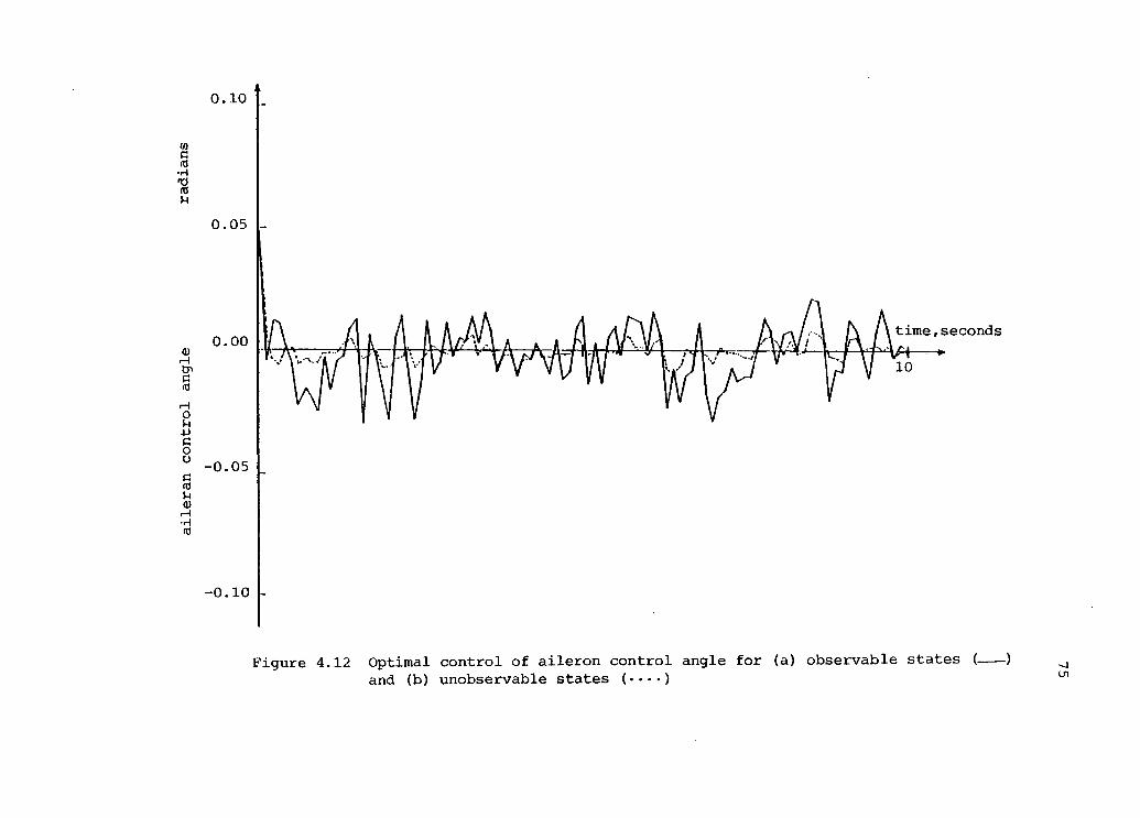
0.10

0.05

0.00

-0.05

-0.10

time, seconds

Figure 4.12 Optimal control of aileron control angle for (a) observable states (..___)and (b) unobservable states ()

76

5. ON NONLINEAR FILTERING AND TRACKING OF TARGET

Among anti-submarine target-motion analysis algorithms for

mobile platforms, one convenient mathematical tracking model con-

sists of describing the target dynamics by a set of state-variable

equations that are driven by a Wiener process. Dynamic motion of

the moving target is generally nonlinear and unobservable; in

passive bearings-only-tracking problems the observations us-

ually appear in the argument of an arc-tangent function. The ex-

tended Kalman filter is a popular method for treating such non-

linear estimation problems [47,48,51,52,55]. However, if non-

linearities are sufficiently important, the estimation error can

be significantly reduced through use of a higher-order estimation

technique.

It is the purpose of this chapter to compare performance

between an extended Kalman filter and a truncated second-order

nonlinear filter as applied to bearings-only-target tracking using

simulation studies. An approach to tracking a maneuvering target

is also considered.

5.1 Modeling in Two-dimensional Space

A two-dimentionsl version of the bearings-only-tracking prob-

lem is considered. A target 0 is moving in relation to an ob-

server in a viscous fluid as shown in Figure 5.1. The control

UT

and UT2

are thrusts in the X and Y direction, respectively.1

Assume that the magnitude of drag force is a [velocity of 0]2

[53,54] where a is a drag coefficient; the direction is opposite

X

77

Velocity

Figure 5.1 Geometrical definition of vector tracking

to the instantaneous velocity vector. Under the assumptions of

A Aplanar motion and constant mass, define x

1= X, x

2= X, x

3= Y.

x4= Y, the state equations of the target motion may be approximated

byx (t) = x

2(t),

1

x2 (t) = -ax2(t) /x22

(t)+x42(t)

+ uT1

,

x3(t) = x

4(t),

x4 (t) = -a x4(t)I

x22(t)+x4

2(t)

+ uT

,

2

with an observed process y(t) of the form

Y(t) = tan-1

x3(t)

x1(t)

(5-1)

(5-2)

Consider from (5-1) and (5-2), the following stochastic dif-

ferential equation:

dx(t) = f(x(t),t)dt + B(t)u(t)dt + G(t)dwt, (5-3)

and an observed stochastic process, y(t) such that

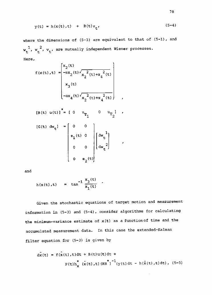
78

y(t) = h(x(t),t) + R(t)vt, (5-4)

where the dimensions of (5-3) are equivalent to that of (5-1), and

wt1, wt

2, vt, are mutually independent Wiener processes.

Here,

and

f(x(t),t) =

x2(t)

-ax2MI/ 2

(t)+x42(t)

x3 (t)

-ax4(t)

2

2(t)+x

4

2(t)

[B(t) u(t)) = 0 0 uTT

1

[G(t) dwt] = O 0

e1(t) 0

O 0

O e2(t)

h(x(t),t) = tan-1

x3(t)

x 1(t)

lwt11dw

t2

2

Given the stochastic equations of target motion and measurement

information in (5-3) and (5-4), consider algorithms for calculating

the minimum-variance estimate of x(t) as a function of time and the

accumulated measurement data. In this case the extended-Kalman

filter equation for (5-3) is given by

dx(t) = f(x(t),t)dt + B(t)u(t)dt +

* ^ * -1P(t)hx (x(t),t)(RR ) (y(t)dt - h(X(t),t)dt), (5-5)

* ^

P(t) = fx(x(t),t)P(t) + P(t)f

x(x(t),t) + G(t)G(t)

* *-P(t)hx (x(t),t)(RR ) hx(x(t),t)P(t),

x(0) = E[x(0)] = x0, P(0) = Cov[x0x0

],

79

(5-6)

Df(where, for any integrable random process x(t), fx

(0)c*

-)= and denote

E[x(t)1Y(s), 0 < s < t] by R(t) or Et[x(t)] and P(t) is the error

covariance matrix. The extended Kalman filter is a useful method

for considering nonlinear estimation problems. If nonlinearities

are important, the unobservable state-estimation error can be re-

duced through use of higher-order estimation methods. Simulation

experiments with the truncated,second-order,nonlinear, filter [55,

79,80] clearly show that it may improve the estimates compared to

the extended Kalman filter.

In general, the conditional-mean estimate Et[x(t)] satisfies

the stochastic equation

dEt[x(t)] = E

t[f(x(t),t)]dt + B(t)u(t)dt

+ fEt[x(t)h (x(t),t)]

E t[x (t) ]E t[h* (x (t) , t) 1 }(RR*

)

-1dvt,

where the innovations process corresponding to (5-7) is.

(5-7)

= y(t) - Et[h(x(t),t)]. (5-8)

The high-order estimation equation for (5-7) can be approximately

obtained as follows. The truncated second-order nonlinear filter

was developed by Bass, et al., [79], and independently Jazwinski

[55]. This filter carries to second order, whereas third and

higher order central moments are neglected. Recently Henriksen [80]

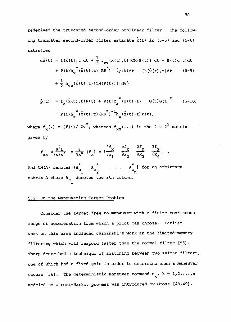
80

rederived the truncated second-order nonlinear filter. The follow-

ing truncated second-order filter estimate x(t) in (5-5) and (5-6)

satisfies

dx(t) = f(x(t),t)dt +1

fxx

(x(t),t)(CM(P(t))]dt + B(t)u(t)dt

+ P(t)hx

*

(x(t),t)(RR*

)

-1{y(t)dt - [h(X(t),t)dt (5-9)

+1hxx(x(t),t)[CM(P(t))]]dt}

I5(t) = fx((t),t)P(t) + P(t)f

x*(x(t),t) + G(t)G(t)* (5-10)

P(t)hx*(x(t),t)(RR

*)

-1hx(x(t),t)P(t),

where fx() = af()/ ax

*, whereas f

xx(.,.) is the 2 x 2

2matrix

given by

32f

afx

afx

afx

afx

f =a

(f x) [

xixx axax ax x 3 bc2

ax3

ax4

'

* * *

And CM(A) denotes [Ac

Ac

. . . Ac

] for an arbitrary1 2 n

matrix A where Ac.

denotes the ith column.1

5.2 On the Maneuvering Target Problem

Consider the target free to maneuver with a finite continuous

range of acceleration from which a pilot can choose. Earlier

work on this area included Jazwinski's work on the limited-memory

filtering which will respond faster than the normal filter [55].

Thorp described a technique of switching between two Kalman filters,

one of which had a fixed gain in order to determine when a maneuver

occurs [56]. The deterministic maneuver command uk, k = 1,2,...,n

modeled as a semi-Markov process was introduced by Moose [48,49].

81

The work of Sworder, et al., [57,58] is aimed primarily at the

development of an adaptive control system for linear systems

in which parameters may jump abruptly. Friedland introduced

properties of the separate-bias estimation technique including

the interpretation of the result as the estimation of a constant

embedded in white noise [59]. This method of separating the esti-

mation of the bias variables that are unknown constants from

the linear dynamic variable was presented. Another useful ap-

proach was presented by Mehra, et al., [60], Wilsky, et al., [61],

and Chan, et al., [62] using evaluation of the properties of the

residual sequence (innovations process).

Suppose this target is maneuvering; then one can examine the

possibility of the target for velocity change and course change

during the certain small time interval At. Since the maneuvering

is unknown, it makes sense, from a knowledge of the performance

capabilities and operating patterns of target, to analyze the

measurement information for observations given assumptions and cur-

rent estimate of all relevant quantities. If the target is maneu-

vering at an average speed in a certain direction, the acceleration

forces u(t) must be equal to drag forces to each direction, or

uTl

(t) = a Et(x

2(t))/ 'x 2

(t)+xt2(t)

a x2(t)iiX 2 (t)+; 2 (t) '

2 2 4

uT2

2

(t) = a Et(x

4(t) x 1'1,c2

(t)+x2(t)

]-1. a x4

(t) 'i.12(t)+X2 (t)

4 2 4

The filter performs well if there are no modeling errors; then

the computed error covariance P(t) becomes small, and the filter

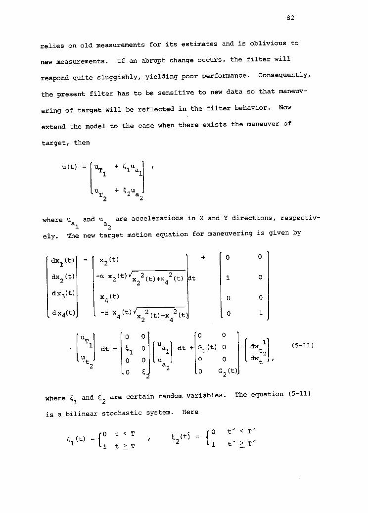
82

relies on old measurements for its estimates and is oblivious to

new measurements. If an abrupt change occurs, the filter will

respond quite sluggishly, yielding poor performance. Consequently,

the present filter has to be sensitive to new data so that maneuv-

ering of target will be reflected in the filter behavior. Now

extend the model to the case when there exists the maneuver of

target, then

u(t) = um +l11

[ uT2+

1 a1

2ua2

where u and ua2

are accelerations in X and Y directions, respectiv-a1

ely. The new target motion equation for maneuvering is given by

dx (t)

dx2(t)

dx3(t)

dx4(t)

T1

ut2

x2 (t)

-a x2(t)

x4(t)

, -a x4

dt +

dt

+

0

G1(t)

0

0 G2

1

0

0

0

(t),

1

1dw

t2

dwt

(5-11)

,

2

2(t)+x

4

2(t)

(t)V 2

0 0

10

0 0

0 E4

(t)+x

al

ua2

4

2(t)

dt

where E1

and E2are certain random variables. The equation (5-11)

is a bilinear stochastic system. Here

(t)t < T

(t0 t' < T

E1 2

5 =

1 t > T 1 t" T"

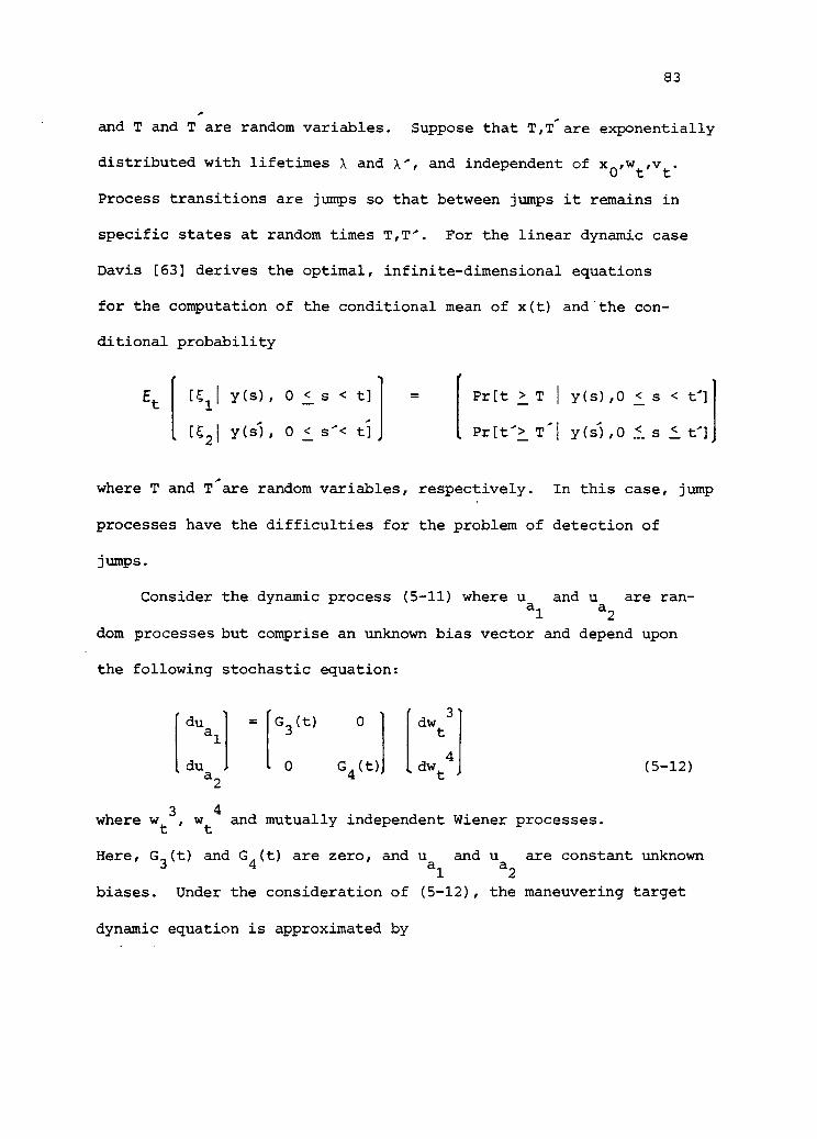
83

and T and T are random variables. Suppose that T,T are exponentially

distributed with lifetimes A and A", and independent of xo,wt,vt.

Process transitions are jumps so that between jumps it remains in

specific states at random times T,T'. For the linear dynamic case

Davis [63] derives the optimal, infinite-dimensional equations

for the computation of the conditional mean of x(t) and the con-

ditional probability

[

Et

[

11y(s), 0 < s < t] = Pr[t > T

1 Y(s),0 < s < tl

H21 Y(i5, 0 < s"< t] Pr[t"> T-1 y(s),0 < s < tl

where T and Tare random variables, respectively. In this case, jump

processes have the difficulties for the problem of detection of

jumps.

Consider the dynamic process (5-11) where u and u are ran-al a2

dom processes but comprise an unknown bias vector and depend upon

the following stochastic equation:

= 0 1 idwt3all

dua

0 G4(t) dwt

4

2

where wt3, wt4 and mutually independent Wiener processes.

(5-12)

Here, G3(t) and G

4(t) are zero, and u

aand u

aare constant unknown

l 2

biases. Under the consideration of (5-12), the maneuvering target

dynamic equation is approximated by

dx1(t)

dx2 (t)

dx3 (t)

dx4(t)

dual

(t)

dua(t)2

x2(t)

- a x2 (t) 1/x

2

2(t)+x

2(t)+u

a(t)

41

x4(t)

- a x4(t) Yx 2

(t)+x2(t)+u (t)

2 4 a1

0

0

0

1

1

dt

uT1

uT2

dt

84

0

G1 (t)

0

0

0

0

0

0

0

G2(t)

0

0

0

0

0

0

G3(t)

0

0

0

0

0

0

G4(t)

1dw

t

dwt

2

dwt

3

4dw

t

(5-13)

And observation is given by

y(t) = h(x(t) ,t) + Rvt

Here, also assumed wt1, wt2 , wt

3, wt li

4, are mutually independent.

Let (5-13) denote

(5-14)

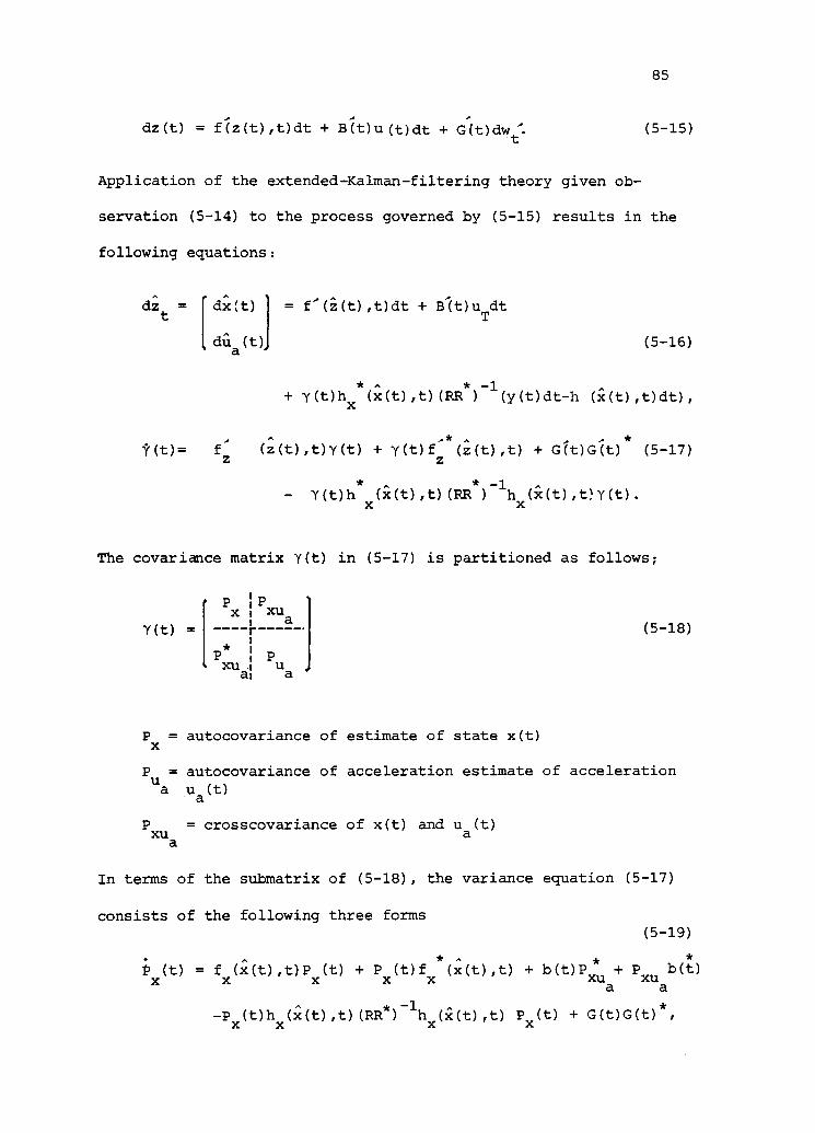
dz(t) = f(z(t),t)dt + 13(t)u(t)dt + G(t)dw;.

85

(5-15)

Application of the extended-Kalman-filtering theory given ob-

servation (5-14) to the process governed by (5-15) results in the

following equations:

dZt

= dx(t) = f-(2(t),t)dt + B(t)u dt

daa(t) (5-16)

+ y(t)hx

*(x(t),t)(RR

*)

-1(y(t)dt-h (X(t),t)dt),

. . ,.

/(t)= fz

(z(t),t)Y(t) + Y(t)f*

z(z(t),t) + Gt)G(t)

*(5-17)

- Y(t)h*

x(x(t),t)(RR

*)

-1hx(x(t),t)Y(t).

The covariance matrix Y(t) in (5-17) is partitioned as follows;

Y

px Pxua

(t) =*

xu ua a

Px= autocovariance of estimate of state x(t)

(5-18)

Pu= autocovariance of acceleration estimate of acceleration

a ua(t)

P = crosscovariance of x(t) and ua(t)

xua

In terms of the submatrix of (5-18), the variance equation (5-17)

consists of the following three forms(5-19)

*

x(t) = f

x(x(t),t)P

x(t) + P (t) f (x(t),t) + b(t)P

xua+ P

xuab(t)

x x

-Px(t)h

x(x(t),t)(RR*)-1h

x(ii(t),t) P

x(t) + G(t)G(t)*,

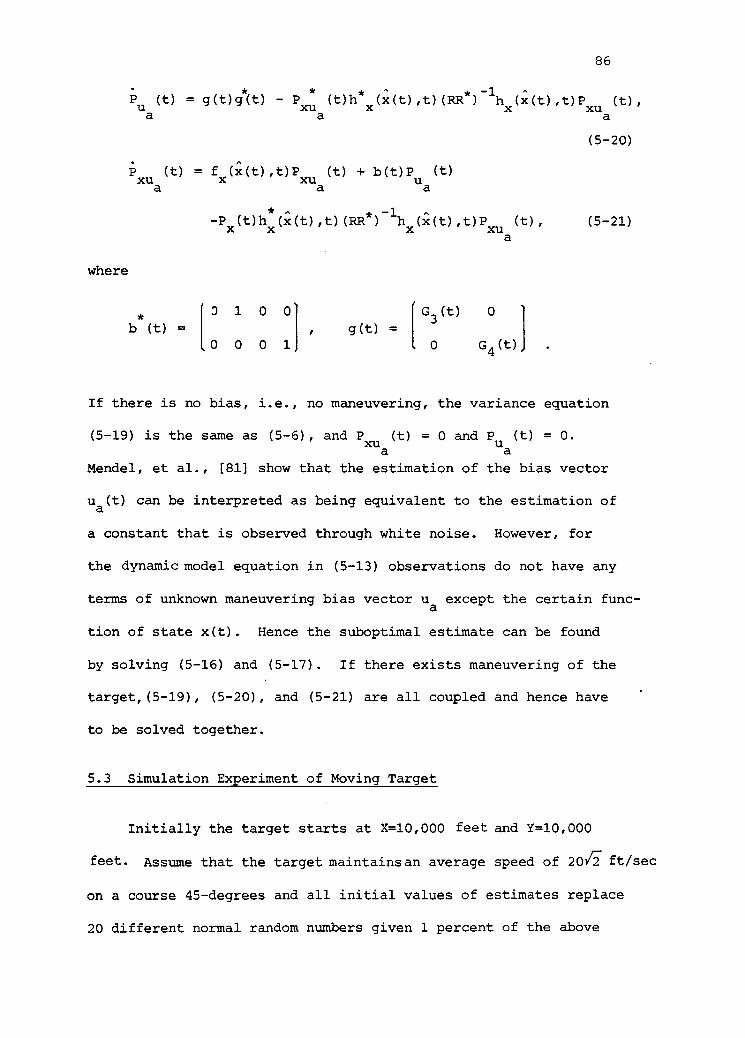
where

86

Pua

(t) = g(t)g(t) - Pxu

(t)h*x(x(t),t)(RR

* -1) h

x(x(t),t)P

xu(t) ,

a a

(5-20)

Pxu

(t) = fx(X(t),t)P

xu(t) + b(t)P

ua(t)

a a

* --P

x(t)h

x(x(t),t)(RR

*)

-1hx(x(t),t)P

xu(t), (5-21)

a

1 0 0 G3 (t) 0

b (t) = , g(t) =0 0 0 1 0 G4 (t) .

If there is no bias, i.e., no maneuvering, the variance equation

(5-19) is the same as (5-6), and Pxu (t) = 0 and Pu (t) = 0.a a

Mendel, et al., [81] show that the estimation of the bias vector

ua(t) can be interpreted as being equivalent to the estimation of

a constant that is observed through white noise. However, for

the dynamic model equation in (5-13) observations do not have any

terms of unknown maneuvering bias vector uaexcept the certain func-

tion of state x(t). Hence the suboptimal estimate can be found

by solving (5-16) and (5-17). If there exists maneuvering of the

target,(5-19), (5-20), and (5-21) are all coupled and hence have

to be solved together.

5.3 Simulation Experiment of Moving Target

Initially the target starts at X=10,000 feet and Y=10,000

feet. Assume that the target maintains an average speed of 20 ii ft/sec

on a course 45-degrees and all initial values of estimates replace

20 different normal random numbers given 1 percent of the above

87

specified values. All the computer runs are made with 20 different

runs to obtain the root-mean-square-error statistics associated

with each geometry. The results present for root-mean-square

velocity and position to the extended Kalman filter and the trun-

cated second-order filter, respectively. The results of the esti-

mation processes are presented by Figure 5.2, 5.3, 5.4. In the

weighting of the observation data it is assumed that the noise

level on the bearing information is 0.05 radians on the bearing

observations. The dynamical noise levels are 1 percent of velocity.

The simulation results presented here demonstrate that the extended

Kalman filter and truncated second-order filter are stable esti-

mation algorithms forbearing only target motion analysis. Further-

more, Figure 5.4 reveals that the truncated second-order filter

is much better than the extended Kalman filter for the time duration

of the first 15 seconds. After 15 seconds the extended Kalman

filter performs better than the truncated second-order filter be-

cause the higher nonlinearity in (5.3) disappears. It means that the

target motion has reached steady state after about 15 seconds.

The second simulation example is similar to the first, the

target maintains an average speed of 20/i ft/sec. Here if it is

assumed that all system parameters are given constants, the starting

time for turns and general maneuvering can be detected from the inno-

vations process. All conditions are the same as the first, and

assume x5(0) = 0, x6(0) = 0 ft/sec

2in equation (5-13).

According to equation (5-13) and (5-14), all cases are tested

with the extended Kalman filter and the truncated second-order

88

filter. The results of a fast 90-degree right turn and the maneu-

vering target for the new average speed 301/ ft/sec after about

50 seconds are presented in Figures 5.5, 5.6, 5.7. In this plot,

the exact target track, and the estimated track using the extended

Kalman filter and the truncated second-order filter, respectively

are shown as the estimate X, Y ranges of each direction, and the

estimated range of the target. The presence of target-estimation

delay to compare with the exact target track is visible. The simu-

lation results show that with abrupt changes in bearing and velocity

of a target, the results of the extended Kalman filter according

to equation (5-13) and (5-14) indicate the effectiveness of the

new technique which promises improved tracking for maneuvering tar-

get.

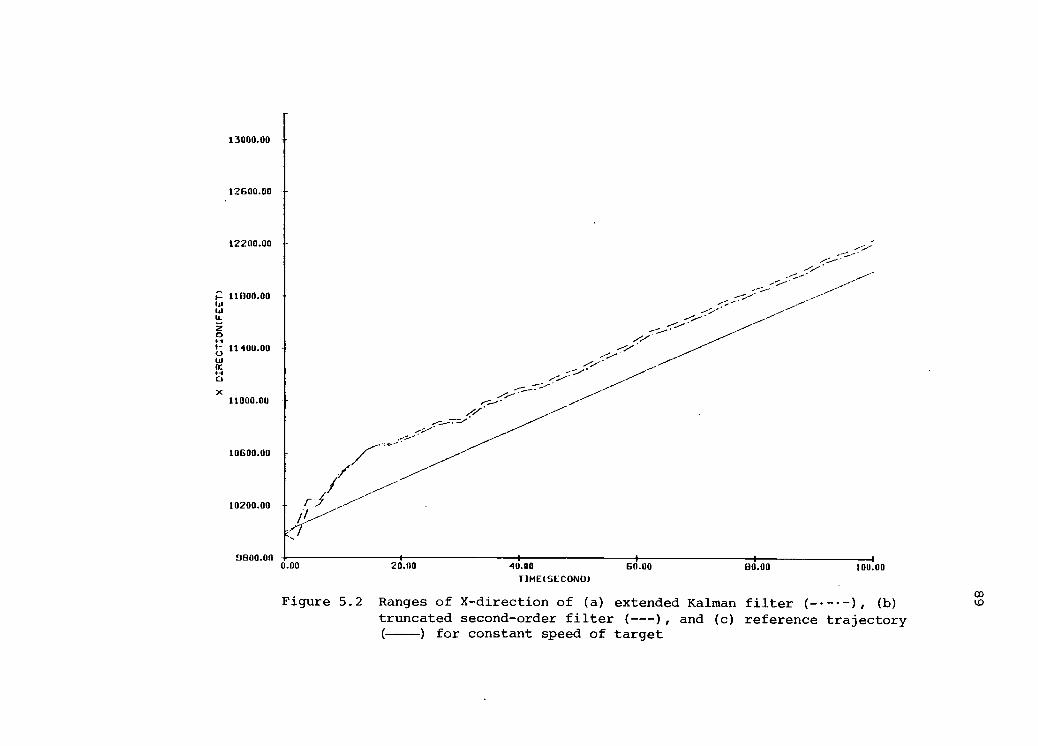
13000.00

12600.00 -

12200.00

11000.00

11400.00

11000.00 !--4/

10600.00

10200.00

0E100.000.00 20.00 40.00 60.00

TIME(SECONE)00.00 100.00

Figure 5.2 Ranges of X-direction of (a) extended Kalman filter (--- -), (b)

truncated second-order filter (---), and (c) reference trajectory) for constant speed of target

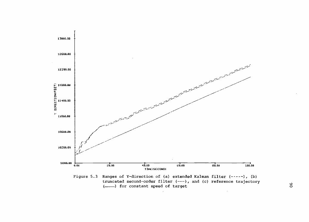
13000.00

12600.00

12200.00.-----"'.----

--.-2-...---

--,...----

111100.00 -.------- ---------

../.:--' ------:%-* ---

--7- -------

----/-...--------

11400.00 -!-----////---L.,

------ ..----

%--- ,----,------ ...---

11000.00..----------.......-

10600.00

10200.00

11E100.000.01)

lJ

20.00 40.001-1146t SECOND)

60.00 110.00 100.00

Figure 5.3 Ranges of Y-direction of (a) extended Kalman filter (- --), (b)truncated second-order filter (---), and (c) reference trajectory

) for constant speed of target

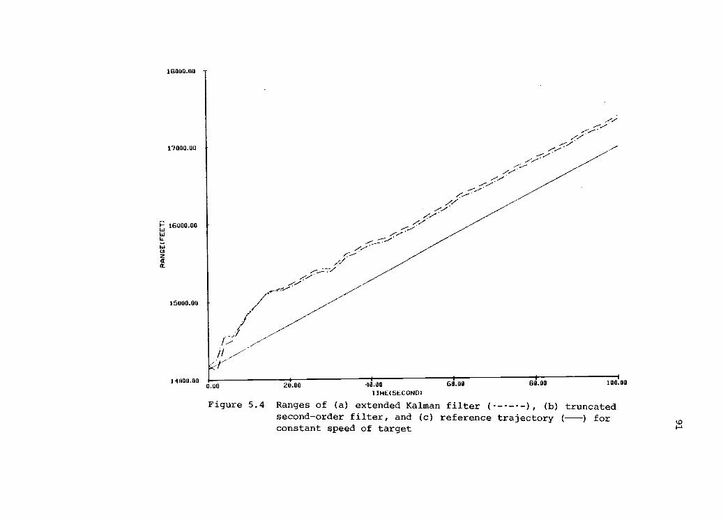
18000.00

17000.00

15000.00

11000.000.00 20.00 10.00 60.00 80.00 100.00

11ME(SECONO)

Figure 5.4 Ranges of (a) extended Kalman filter (- - -), (b) truncatedsecond-order filter, and (c) reference trajectory (---) forconstant speed of target

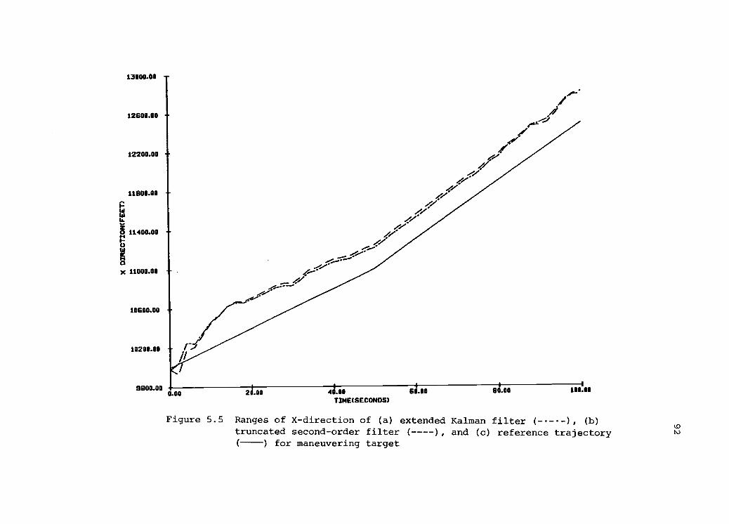
13000.00

12600.00

12200.00

11800.00

g 11400.00

gw

x 11000.00

10600.00

10200.00

8800.00

40'

ii

ii

e/

0.00 20.09 4 .00 60.00TIMEISECONDS)

80.00 100.00

Figure 5.5 Ranges of X-direction of (a) extended Kalman filter (-----), (b)

truncated second-order filter (----), and (c) reference trajectory(----) for maneuvering target

12400.00

12000.00

11600.00

.1%.:......./!---'11200.00 ././ N..-...---

w ,.1,......:1--.

1 10800.00 -!--"' \NI-

,e:''.

N.)- 10400.00

10 000.00

9600.00

9200.000.00 2 .00 40.00 6 .00

TIME(SECONDS)80.00 100.00

Figure 5.6 Ranges of Y-direction of (a) extended Kalman filter (--- -),(b) truncated second-order filter (---), and (c) reference tra-jectory ( ) for maneuvering target

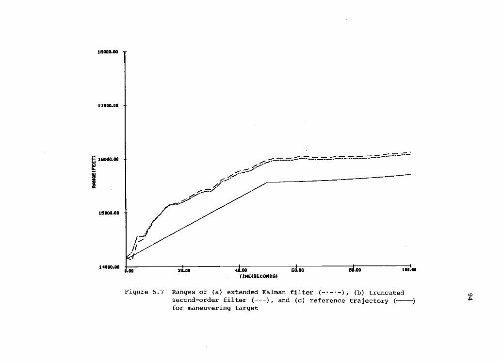
16000.00 -

17000.00

15000.80

14000.00

'7' = --"--- --- ---../,.../

:--*"..01/**

":7*--""

4y.....:-..n/

./.**

.1.---"...--

0.00

...........,.....

20.00 41.00 611.00

TIME(SECONDS)SE CONDS)

100.00

Figure 5.7 Ranges of (a) extended Kalman filter (-----), (b) truncatedsecond-order filter (---), and (c) reference trajectory ( )

for maneuvering target

95

6. CONCLUSIONS

The contribution of this dissertation is in the presentation

of the optimal and the suboptimal control for certain linear sto-

chastic systems with known and unknown random coefficients in the

Bellman-Hamilton-Jacobi equation and related algorithms.

To analyze the optimal control for a linear system with com-

pletely observable random coefficients, the proofs of existence

of optimal control are based on the stochastic version of Bellman's

principle of optimality and Kolodziej's results [29]. The sub-

optimal control for the class of certain stochastic control sys-

tems with unknown coefficients belongs to the coupled bilinear sto-

chastic system is also studied here. The main assumption made is

that a finite-dimensional filter, which is independent of the con-

trol and which gives a good estimate of the unobservable coefficients,

can be found. Structure of this filter is used to construct the

suboptimal control in equation (3-1). For the quadratic cost

function, the explicit formulae describing the control law is de-

rived. The gain of the linear-in-state feedback is a solution to

certain nonlinear partial differential equations.

It is expected that the class of stochastic models, which

satisfy the assumptions made here, includes many of these models

for which there is no existing technique leading to strictly opti-

mal results. The approximate stochastic model investigated with

the stated assumptions produces a close optimal result. The

measurement information about uncertain quantities use E[ztlZt,

0 < t < T], but this conditional estimate could not be used for

96

the exact stochastic model in equation (3-1) since its innovation

process depends upon the feedback control law.

The numerical examples are provided to illustrate the previous

results. The generation of the Wiener process is used for the

random-walk theory with the pseudo-uniform random numbers and the

pseudo-Gaussian random number N(0,1). It turns out that the pseudo-

Wiener process satisfies the general properties of the Wiener pro-

cess and passes some proper random testing methods.

Numerical solution of the Riccati-like equation to the Cauchy

problem suggests the need for more precise numerical methods to

be simulated by digital computer. In general, simulation results

of this type of nonlinear partial differential equation use ex-

cessive computer time.

For bad weather conditions of an aircraft landing system in

wind gusts, the theoretical results of Chapter 3 illustrate the

design procedure of the optimal control. It is found that the sub-

optimal control-design technique to the stochastic-parameter linear

system provides an effective method for choosing the appropriate

stochastic models. Moreover, the simulation results of altitude

of aircraft is almost the same as the exponential, linear -flare

path for safe comfortable landing. The above method can also be

applied to the control problems of longitudinal motion of an air-

craft in gusty wind containing a dynamical feedback controller. It

makes it possible to ensure the proper trajectories of the angle

of attack and the orientation rate for optimal control law of the

elevator control angle and the aileron control angle given a

97

reasonable cost function. The method proposed here can also be

applied to unobservable stochastic systems if there exist the

conditional Gaussian filter and simultaneous solution of certain

nonlinear partial differential equations corresponding to given

stochastic models.

To approximate stochastic models, the suboptimal control in

equation (3-1) is a fruitful area for developing improved control

policies. The suboptimal control has considerable complexity be-

cause of a linear function of observable states and a nonlinear

function of uncertain random parameters. However, this author

believes that suboptimal feedback control presents the most useful

optimization result in stochastic control theory.

It describes the nonlinear target model for an optimal de-

cision algorithm to decide between maneuvering and nonmaneuvering

targets. The extended Kalman filter and the truncated second-

order filter for implementation in anti-submarine warfare, target-

motion analysis are developed and presented in Chapter 5. The

target-motion equation for maneuvering given by (5-12) is modeled

in the form of a bilinear stochastic system when the unknown ac-

celerations are generated from the equation (5-12). The optimal

estimate can produce the solution of (5-16) and (5-17) which have

to be solved together. It may be possible to estimate adaptively

the covariance Y(t), which is dependent on the original states

and a target maneuver. Preliminary work using realistic computer

simulation for no maneuvering indicates that the extended Kalman

filter and the truncated second-order filter accuracies agree to

98

within about 3 percent. Results shown in Figure 5.4 show that the

truncated second-order filter is much better than the extended Kal-

man filter for the time duration of the first 15 seconds. After

15 seconds the extended Kalman filter performs better than the

truncated second-order filter because the nonlinearities (5.3) de-

crease in significance.

This section discusses some special problems that have yet to

be proven in the area of optimal control. For practical appli-

cations of known results in the area of optimal control, it is

necessary to develop efficient numerical technique for solving

nonlinear partial differential equations in (2-18) and (3-19)

which have multi-dimensions.

It would be also interesting to study the problem of optimal

control for stochastic dynamic systems with discrete random coef-

ficients like Markov jump processes. For example if the target

maneuvers, a detector has to estimate the unknown input accelerations

of target motion. The maneuvering characteristic of the target

may be described by the stochastic model provided. Also the

finite-state, continuous-time, Markov process with weak interaction

may be modeled as a singularly perturbed system, such as by queueing

network models of computer systems which accentuates the need for

reduced-order approximations of large-scale Markov chains. The

theoretical results which are provided here may be applied to

the singularly perturbed form to simplify the treatment of cost

equations and decentralized algorithms in optimization problems.

The most important results desired are with respect to more

99

adequate mathematical models that can be used for synthesis of

optimal control laws. The estimate E[zt lYt] is suboptimal in

a sense that the state variable xtalso includes information about

uncertain quantities. However, the contruction of the conditional

estimate is not available with respect to the c- algebra Zt because

of dependence on the feedback control law.

Also, it would be useful to develop conditions of stability

for bilinear stochastic systems governed by nonlinear Ito dif-

ferential equations equipped with random coefficients which have

incomplete state information but to make it available for appropri-

ate feedback control.

100

REFERENCES

1. Fleming, W. H., "Optimal Control of Partially ObservableDiffusions," SIAM J. Control 6, (1968). pp. 194-213.

2. Fleming, W. H., "The Cauchy Problem for Degenerate Para-bolic Equations," J. Math. Mech. 13, (1964), pp. 987-

1008.

3. Fleming, W. H., "Optimal Continuous-Parameter StochasticControl," SIAM Review 11, (1969), pp. 470-509.

4. Fleming, W. H., and Rishel, R. W., Deterministic and Sto-

chastic Optimal Control, (1975), Springer-Verlag,

New York.

5. Kushner, H. J., "On the Dynamical Equations of Conditional

Density Functions with Application to Optimal Stochastic

Control Theory," J. Math Anal. Appl. 8, (1964),

pp. 332-344.

6. Kushner, H. J., "On the Existence of Optimal Stochastic

Controls," SIAM J. Control 3, (1966), pp. 463-474.

7. Wonham, W. M., "On the Separation Theorem of Stochastic

Control," SIAM J. Control 6, (1968), pp. 312-316.

8. Wonham, W. M., "Optimal Stationary Control of Linear Systems

with Dependent Noise," SIAM J. Control 5, (1967),

pp. 486-500.

9. Wonham, W. M., "Random Differential Equation in Control

Theory," in Probabilistic Methods in Applied Mathematics,

Vol. II, (1970)ed. by Bharucha-Reid, New York Academic

Press, pp. 131-242.

10. Balakrishnan, A. V., "Stochastic Control: A Function Space

Approach," SIAM J. Control 10, (1972), pp. 285-297.

11. Balakrishnan, A. V., "Modeling and Identification: A Flight

Control Application," in Theory and Applications of Vari-

able Structure Systems, (1972), ed. by Mohler, R. R. and

Ruberti, A., Academic Press New York, pp. 1-24.

12. Benes, V. E., "Existence of Optimal Stochastic Control Laws,"

SIAM J. Control 9, (1972), pp. 446-472.

13. Belles, V. E., "Existence of Optimal Strategies Based on

Specified Information for a Class of Stochastic Decision

Problems," SIAM J. Control 8, (1970), pp. 179-188.

101

14. Rishel, R. W., "Necessary and Sufficient Dynamic ProgrammingConditions for Continuous Time Stochastic Optimal Con-trol," SIAM J. Control 8, (1970), pp. 559-571.

15. Rishel, R. W., "Optimality of Controls for System with JumpMarkov Disturbances," SIAM J. Control 13, (1975),pp. 338-171.

16. Bismut, J. M., "Linear Quadratic Optimal Stochastic Equationswith Random Coefficients," SIAM J. Control and Optimi-zation 14, (1976) pp. 419-444.

17. Bismut, J. M., "On Optimal Control of Linear StochasticEquations with Linear Quadratic Criterion," SIAM J. Con-trol and Optimization 15, (1977), pp. 1-4.

18. Bismut, J. M., "An Introductory Approach to Duality in Opti-mal Stochastic Control,"SIAM Review 20, (1978), pp. 62-78.

19. Davis, M. H. A., and Varaiya, "Dynamic Programming Conditionsfor Partially Observable Stochastic Systems," SIAM J.Control 11, (1973), pp. 226-261.

20. Davis, M. H. A., "On the Existence of Optimal Policies inStochastic Control," SIAM J. Control 11, (1973), pp. 587-594.

21. Davis, M. H. A., "The Separation Principles in Stochastic Con-trol via Girsanov Solutions," SIAM J. Control and Opti-mization 14, (1976), pp. 176-188.

22. Davis, M. H. A., "The Separation Theorem for Linear Systemswith Quadratic Cost Functions," Publication 72/36 (Lecturenotes), (1972), Departement of Computing and Control,Imperial College, London SW7 2BT.

23. Davis, M. H. A., "Martingale Methods in Stochastic Control,"in Stochastic Control Theory and Stochastic DifferentialSystems, (1979), ed. by Kohlmann, K. and Vogel, W.,Spring-Verlag, New York, pp. 85-117.

24. Eliott, R. J., "The Optimal Control of a Stochastic ControlSystems," SIAM J. Control and OPtimization 15, (1977),pp. 756-778.

25. Eliott, R. J., "A Sufficient Condition for the Optimal Con-trol of a Partially Observed Stochastic System," inAnalysis and Optimzation of Stochastic Systems, (1979)ed. by Jacobs, D. L. R., Academic Press, New York, London.

102

26. Haussmann, U., "On the Existence of Moments of Stationary Lin-ear Systems with Multiplicative Noise," SIAM J. Control12, (1974), pp. 99-105.

27. Haussmann, U., "Optimal Stationary Control with State andControl Dependent Noise," SIAM J. Control 9, (1971),pp. 184-198.

28. Variya, P., "Optimal Control of a Partially Observed Sto-chastic System," Proc. Symp. Appl. Math., (1972), NewYork pp. 173-187.

29. Kolodziej, W. J., "Conditionally Gaussian Process in StochasticControl Theory," (1980), Ph.D. Dissertation, OregonState University, Corvallis, Oregon.

30. Mohler, R. R. and Kolodziej, W. J., "Optimal Control of a Classof Nonlinear Stochastic Systems," IEEE Trans. Auto. Cont.Vol. AC-26, (1981), No. 5, pp. 1048-1054.

31. Mohler, R. R. and Kolodziej, W. J., "An Overview of StochasticBilinear Control Processes," IEEE Trans. Systems, Man andCybernetics, Vol. SMC-10, (1980), No. 12, pp. 913-918.

32. Leitmann, G., "Guaranteed Ultimate Boundness for a Class ofUncertain Linear Dynamic Systems," IEEE, Trans. Auto.Cont., Vol. AC-23, (1978), pp. 1109-1110.

33. Leitmann, G., "On the Efficacy of Nonlinear Control in Uncer-tain Linear Systems," ASME J. Dynamic System, Measurement& Control, Vol. 102, (1981), pp. 95-102.

34. Leitmann, G., "Stabilization of Dynamical Systems under BoundedInput Disturbances and Parameter Uncertainty," inDifferential Games and Control Theory II, (1977), ed. byRoxin, E. O., et al., Marcel Decker, Inc., pp. 47-64.

35. Ahmed, N. U., "Stochastic Control on Hilbert Space for LineaEvolution Equations with Random Operator-Valued Coefficients,"SIAM J. Control and Optimzation 19, (1981), No. 3,pp. 401-430.

36. Athans, M., Ku, R., and Gershwin, S. B., "The UncertaintyThreshold Principle: Some Fundamental Limitations ofOptimal Decision Making under Dynamic Uncertainty,"IEEE Trans. Auto. Contr., Vol. AC-22, (1977), pp. 491-495.

37. Ku, R. and Athans, M., "Further Results on the UncertaintyThreshold Principle," IEEE Trans. Auto. Contr., Vol.AC-22, (1977), pp. 866-868.

103

38. Bensoussan, A. and Viot, B., "Optimal Control of StochasticLinear Distributed Parameter Systems," SIAM J. Control13, (1975), pp. 904-906.

39. McLane, P., "Optimal Stochastic Control of Linear Systemswith State-and Control Dependent Disturbances," IEEETrans. Auto. Contr., Vol. AC-16, (1971), pp. 793-798.

40. McLane, P., "Linear OPtimal Stochastic Control using Instane-ous Output Feedback," Int. J. Control, Vol. 13, (1971),pp. 383-396.

41. Bruni, C., Dipillo, G., and Koch, G., "Bilinear Systems: AnAppealing Class of "Nearly Linear" System in Theoryand Applications," IEEE Trans. Auto. Contr., Vol. AC-19(1974), pp. 334-348.

42. Sincovec, R. F., and Madsen, N. K., "Solution for NonlinearPartial Differential Equations," ACM Trans. on Math.Software, (1975), pp. 232-260.

43. Balakrishnan, A. V., Stochastic Filtering and Control, Opti-mization, (1981), Software, Inc., Los Angeles.

44. Grishin, V. P., "On a Calculation Method Related to a Processof Automatic Adaptation," Automatic Remote Control, (1963),No. 12, pp. 1502-1509.

45. Holley, W. E., and Bryson, A. E., "Wind Modeling and LateralControl for Automatic Landing," AIAA J. Spacecraft andRockets, (1977), Vol. 14, No. 2, pp. 65-72.

46. Dryden, H. L., "Turbulence Investiation at the National Bureauof Standards," Proc. 5th International Congress of Ap-plied Mechanics, 1938, p. 365.

47. Singer, R. A., "Estimating Optimal Tracking Filter Performancefor Manned Maneuvering Targets," IEEE Trans. Aerosp.Electron. Syst., Vol. AES-6, (1970), pp. 473-483.

48. Moose, R. L., Vanlandingham, H. F., and McCabe, D. H., "Model-ing and Estimation for Tracking Maneuvering Targets,"IEEE Trans. Aerosp. Electron. Syst., Vol. AES-15, (1979),pp. 448-456.

49. Gholson, N. H., and Moose R. L., "Maneuvering Target TrackingUsing Adaptive State Estimation," IEEE Trans. Aerosp.Electron. Syst., Vol. AES-13, (1977), pp. 310-319.

50. Chan, Y. T., Hu, A. G. C., and Plant, J. B., "A Kalman FilterBased Tracking Scheme with Input Estimation," IEEE Trans.Aerosp. Electron. Syst., Vol. AES-15, (1979), pp. 237-244.

104

51. Chou, S. I., "Some Drawbacks of Extended Kalman Filtering inASW Passive Angle Tracking," in Advanced in Passive Tar-get Tracking. Moneterey, CA, (1977): Naval Post Gradu-ate School, pp. 76-113.

52. Aidala, V. J., "Behavior of the Kalman Filter Applied toBearings-Only Target Motion Tracking," ibid. as 51,pp. 1-30.

53. Kerr, K. P., "Determing Hydrodynamic Coefficients by Meansof Slender Body Theory," Lockheed Missiles and SpaceCompany, (1959), IAD/790.

54. Hess, J. L., "Calculation of Potential Flow about Bodies ofRevolution Having Axes Perpendicular to the Free StreamDirection," Douglas Aircraft Company, Report No. ES 29812,(1960).

55. Jazwinski, A. H., Stochastic Processes and Filtering Theory,Academic Press, (1970), New York.

56. Thorp, J. S., "Optimal Tracking of Maneuvering Targets,"IEEE Trans. Aerosp. Electron. Syst., Vol. AES-9, (1973),pp. 512-519.

57. Sworder, D. D., "Bayes' Controller with Memory for a LinearSystem with Jump Parameters," IEEE Trans. Auto. Contr.,Vol. AC-17, (1972), pp. 119-112.

58. Sworder, D. D. and Robinson, V. G., "Feedback Regulators forJump Parameter System with State and Control DependentTransition Rates," IEEE Trans. Auto. Contr., Vol. AC-18,1973, pp. 355-360.

59. Friedland, B., "Notes on Separate-Bias Estimation," IEEE TransAuto. Contr., Vol. AC-23, (1978), pp. 735-738.

60. Mehra, R. K. and Peschon, J., "An Innovations Approach toFault Detection and Diagnosis in Dynamic Systems,"Automatica, Vol. 7, (1971), pp. 637-640.

61. Willsky, A. S. and Jones, H. L., "A Generalized LikelihoodRatio Approach to the Detection and Estimation of Jumpsin Linear SYstems," IEEE Trans. Auto. Contr., Vol.AC-21, (1976), pp. 108-112.

62. Chan, Y. T., Plant, J. B. and Bottomley, J. R. T., "A KalmanTracker with a Simple Input Estimator," IEEE Trans.Aerosp. Electron. Syst., Vol. AES-18, (1980), 235-240.

105

63. Davis M, H. A., "The Application of Nonlinear Filtering toFault Detection in Linear Systems," IEEE Trans. Auto.Contr., Vol. AC-20, (1975), pp. 257-259.

64. Liptser, R. S., and Shiryayev, A. N., Statistics of RandomProcesses I: General Theory, (1977), Springer-Verlag,New York.

65. Liptser, R. S., and Shiryayev, A. N., Statistics of RandomProcesses II: Applications, (1978), Springer-Verlag,

New York.

66. Mohler, R. R., Bilinear Control Processes, (1973), AcademicPress, New York.

67. Mohler, R. R., Barton, C. F., and Hsu, C. S., "T and B CellModels in the Immune System,"in Theoretical Immunology,ed. by Bell, G., et al., (1978), Marcel Dekker,New York.

68. Mohler, R. R., and Frick, P. A., "Bilinear Demographic Con-trol Process," Int. J. Policy Anal. Inform. Syst.,Vol. 2, (1979), pp. 57 -70.

69. Kallianpur, G., Stochastic Filtering Theory, (1980), Springer-Verlag, New York.

70. Feller, W., An Introduction to Probability Theory and itsApplication, 3rd ed., (1968) Vol. 1, John Wiley & Sons,

Inc., New York.

71. Gear, C. W., Numerical Initial Value Problems in OrdinaryDifferential Equations, (1971), Prentice Hall, EnglewoodCliffs, N.J..

72. Hindmarsh, A. C., "Gear b: Solution of Ordinary DifferentialEquation Having Bounded Jacobian," Rep. UCID-30059,(1972), Lawrence Livermore Lab., Livermore, CA.

73. Hindmarsh, A. C., "Gear: Ordinary Differential EquationSolver," Rep. UCID-30001, (1972), Lawrence LivermoreLab., Livermore, CA.

74. Massey, F. J. Jr., "The Kolmogorov-Smirnov Test for Goodnessof Fit," J. Amer. Stat. Assn., (1951), 46, pp. 68-78.

75. Frick, P. A., "On Walsh Noise: Its Properties and Use inDynamic Stochastic Systems," IEEE Trans. on Sys., Man,and Cyber., Vol. SMC-9, (1979), No. 8, pp. 411-419.

76. Davis, M. H. A., Linear Estimation and Stochastic Control,John Wiley & Sons, Inc., (1977), New York.

106

77. Taylor, H. M., A First Course in Stochastic Process, (1975),Academic Press.

78. Etkin, B., Dynamics of Atmospheric Flight, (1972), JohnWiley and Sons, Inc., New York, pp. 158-195.

79. Bass, R. D., Norum, V. D., and Swartz, L.,channel Nonlinear Filtering," J. Math.16, (1966), pp. 152-164.

80. Henriksen, R., "The Truncated Second-OrderRevisited," IEEE Trans. Auto. Contr.,pp. 247-251.

"Optimal Multi-Anal. Appl., Vol.

Nonlinear FilterVol. AC-27, (1982),

81. Mendel, J. M., and Washburn, H. D., "Multistage Estimationof Bias States," in Proc. (1976) IEEE Conf. on Decisionand Control, pp. 629-630.