Optimization of soil-adjusted vegetation indices

ELSEVIER

Optimization of Soil-Adjusted Vegetation Indices

Genevibve Rondeaux,* Michael Steven,* and Fr6d6ric Baret t

T h e sensitivity of the normalized difference vegetation index (NDVI) to soil background and atmospheric effects has generated an increasing interest in the development of new indices, such as the soil-adjusted vegetation index (SA VI), transformed soil-adjusted vegetation index (TSA VI), atmospherically resistant vegetation index (AR VI), global environment monitoring index (GEMI), modified soil-adjusted vegetation index (MSA VI), which are less sensitive to these external influences. These indices are theoretically more reliable than ND VI, although they are not yet widely used with satellite data. This article focuses on testing and comparing the sensitivity of NDVI, SAVI, TSAVI, MSA VI and GEMI to soil background effects. Indices are simulated with the SAIL model for a large range of soil reflectances, including sand, clay, and dark peat, with additional variations induced by moisture and roughness. The general formulation of the SA VI family of indices with the forvn VI = (NIR - R) / (NIR + R + X) is also reexamined. The value of the parameter X is critical in the minimization of soil effects. A value of X = 0.16 is found as the optimized value. Index performances are compared by means of an analysis of variance.

I N T R O D U C T I O N

During the last decade, vegetation indices based on simple combinations of visible and near-infrared reflectances, such as the normalized difference vegetation index (NDVI) and simple ratio (SR), have been widely used by the remote sensing community to monitor vegetation from space, both on regional and global scales. These indices correlate well with foliage density, but

*Geography Department, University of Nottingham, Notting- ham, UK

tlNRA, Station de Bioclimatologie, Montfavet, France

Address correspondence to Dr. Genevieve Rondeaux, Geography Department, University of Nottingham, Nottingham NG7 2RD, U.K.

Received 2 August 1994; revised 27July 1995.

REMOTE SENS. ENVIRON. 55:95-107 (1996) ©Elsevier Science Inc., 1996 655 Avenue of the Americas, New York, NY 10010

are also sensitive to three main external factors: solar and viewing geometry, soil background, and atmospheric effects. Responses to all three factors are complex, intricately coupled, and dependent on surface characteristics (Qi et al., 1993). Several new indices, such as SAVI (soil-adjusted vegetation index; Huete, 1988) and ARVI (atmospherically resistant vegetation index; Kaufman and Tanr~, 1992) or combinations of both (SARVI; Kaufman and Tanr6, 1992), have been developed in an attempt to minimize these influences. The biophysical explanation of the relations between vegetation indices and observable vegetation phenom- ena is still subject to much discussion, however (Baret and Guyot, 1991, Sellers et al., 1992, Clevers and Ver- hoef, 1993). Although these indices appear to be more reliable and less noisy than the NDVI, they are not widely used except in theoretical studies. The NDVI seems still to be the leading index in remote sensing applications. The reason for this may be either the other indices' more complex formulation or the fact that they have not been convincingly demonstrated to improve on the NDVI in the assessment of vegetation parameters. This article focuses on testing and comparing the sensitivity of the different indices to soil background effects.

The spectral reflectance of a plant canopy is a combination of the reflectance spectra of plant and soil components, governed by the optical properties of these elements and photon exchanges within the canopy. As the vegetation grows, the soil contribution progressively decreases but may still remain significant, depending on plant density, row effects, canopy geometry, wind effects, and so on. In this article soil reflectance properties and variations are summarized and the range of current vegetation indices are briefly reviewed. Values of the various vegetation indices are then simulated for the growth of a typical healthy green canopy, using several soil backgrounds incorporating a wide range of soil reflectances.

0034-4257 / 96 / $15.00 SSDI 0034-4257(95)00186-5

96 Rondeaux et al.

SOIL COLOR AND SOIL REFLECTANCE SPECTRA

The wide variety of soils encountered on the Earth's surface, subject to continuous environmental and temporal variations, has never led to an easy classification of the different soils. The color of the soil, which is closely related to important soil properties, such as soil composition and soil moisture, has appeared to be a more practical way of soil identification. Color classification is often done by means of the U.S. "Munsell Soil Color Charts" atlas (Soil Survey Staff, 1975), which is based on visual observation. This concept of color is described by the colorimetric system, which character- izes every color as a combination of the three primary colors: red, green, and blue. These three coordinates may then be rearranged in the three-dimensional (3D) color space as intensity (or brightness), hue, and saturation (Escadafal, 1993). The development of new instru- ments and remote sensing techniques has added a new dimension by providing soil spectra not only in the visible wavelengths but also in the near- and middle- infrared regions, thus obtaining complementary information about the soil properties (Stone et al., 1980). Thus, the use of remote sensing has undeniably given a new perspective to soil surveys, but has also created a need to be precise when using the term "color."

In general, soil reflectance is relatively low (<10%) in the blue channel, but increases monotonically with wavelength through the visible and near-infrared regions. These optical properties vary with each soil and its complex composition, however. The major soil components are inorganic solids (minerals); organic matter (humus, roots, decaying plant residue, living soil organ- isms); air, and water. Mineral soils by definition contain less than 20% organic matter and cover over 95% of the world land surface (Irons et al., 1989). They may be classed on a textural basis according to the propor- tions of sand, silt, and clay. Organic matter can strongly influence soil reflectance. Humus compounds especially give a dark coloration (Curran et al., 1990), resulting in a general tendency to decrease reflectance throughout the spectrum. The form or decomposition stage of organic material is critical, however, in that less-decomposed organic materials have a much higher reflectance in the near-infrared region than highly decomposed materials (Stoner et al., 1980). Water is also a very important factor, and an increase of the moisture content results in a general decrease of the reflectance. In the visible and near-infrared regions the fraction of reflected radiation changes when air-particle interfaces are replaced by air-water-particle interfaces, whereas in the middle- infrared region the reflectance is controled by water absorption bands.

For remote sensing purposes, soil components are generally grouped into three characteristics: color, roughness, and water content. Roughness also has the

effect of decreasing reflectance because of an increase of multiple scattering and shadowing. Understanding the interactions of solar radiation with soil has led to mathematical models to predict the bidirectional reflectance over bare soils (Irons et al., 1989, Curran et al., 1990, Cierniewski and Courault, 1993). Models ade- quately describe the multiple scattering according to the size and characteristics of soil particles (assuming simple geometric shapes), but more difficulty occurs when introducing soil moisture and organic content. A more realistic approach to soil reflectance is at present only possible by introducing semi-empirical parameters into the models (e.g., SOILSPECT; Jacquemoud et al., 1992).

Analysis and experimental studies indicate that for a given type of soil variability, the soil reflectance (p) at one wavelength is often functionally related to the reflectance in another wavelength (Jasinki and Eagleson, 1989). In many cases, the relation can be approximated by a simple linear expression:

p(22) = ap(2~) + b (1)

where the slope a and intercept b are coefficients dependent on both the wavelengths (21, 3.2) and the type of variability. Thus, variation of any one soil parameter can lead to a representative "line" in a two-dimensional scattergram (3.1 versus 3,2). For red-infrared scattergrams this line is called the "soil line," and is used as a base or reference line in studies of vegetated areas (Huete, 1988; Jasinki and Eagleson, 1989; Baret and Guyot, 1991). The problem is that real soil surfaces are heterogeneous and contain a composite of several types of variability, which may be due to soil type, moisture content, roughness, and also to view-illumination geometry. Jasinki and Eagleson (1989) showed three hypo- thetical visible-infrared scattergrams in which only one soil parameter is allowed to vary at a time, resulting in three lines: a soil mineral line, a soil moisture line, and a soil shadow line (from roughness). When varying all three parameters together, the composite soil line is generally linear in the mean although considerable scatter can exist. A unique soil line will exist only if either one type of soil variability dominates, or the scatter due to the different types of soil variability act in the same direction (Jasinki and Eagleson, 1989).

Vegetation Indices Spectral vegetation indices (VIs) use the well-known characteristic shape of the green vegetation speetrmn by combining the low reflectance in the visible part of the spectrum with the high reflectance in the near- infrared. The combination may be in the form of a ratio, a slope, or some other formulation. Indices may be broadly separated into three categories: 1) intrinsic indices (such as the simple ratio and the NDVI), which do

Soil-Adjusted Vegetable Indices 97

not involve any external factor other than the measured spectral reflectances; 2) soil-line related indices, which include soil-line parameters, such as the perpendicular vegetation index (PVI), the weighted difference vegetation index (WDVI, Clevers and Verhoef, 1993), the soil-adjusted vegetation index or SAVI (Huete, 1988), the transformed SAVI (TSAVI; Baret and Guyot, 1991), and the modified SAVI (MSAVI; Qi et al., 1994); and 3) atmospheric-corrected indices such as ARVI (Kauf- man and Tanr6, 1992) and GEMI (Pinty and Verstraete, 1992). The characteristics and use of each group of indices are described below.

Intrinsic Indices

The simple ratio (SR) = NIR / R, and the normalized difference vegetation index, NDVI = (NIR - R) / (NIR + R), in which NIR and R are, respectively, the reflectances in the near-infrared and red channels, were developed from channels 5 and 7 of the Landsat MSS (MultiSpec- tral Scanner). Their use was rapidly extended to other satellite visible-infrared sensors (Landsat TM, NOAA- AVHRR, SPOT HRV) and also to airborne sensors and high spectral resolution radiometers.

Their popularity comes from their ability to monitor global changes in vegetated areas. These indices are very well related to vegetation amount until saturation at full canopy cover and are therefore also related to the biophysical properties of plant canopies, such as the absorbed photosynthetically active radiation, efficien- cies, and productivity. It has also been shown on experimental data (Steven et al., 1992) that any combination of two thematic mapper bands in an NDVI formulation shows a qualitatively similar relationship to the amount of vegetation, with only a subtle difference between the color sensitivity in the indices; therefore this concept can be extended beyond the two spectral bands normally used.

The intrinsic indices, however, such as NDVI, are extremely sensitive to soil optical properties, and are difficult to interpret with low vegetation cover when the soil is unknown.

Indices Us ing the Soil Line

The relationship between near-infrared and visible reflectances from bare soils is generally linear, and several vegetation indices have been developed using the coefficients of this relationship. Such indices attempt to reduce the influence of the soil by assuming that most soil spectra follow the same soil line. The PVI (or its successor the WDVI) expresses the distance between canopy R and NIR reflectances and the soil line. Al- though bet ter than NDVI at low vegetation densities, PVI is still significantly affected by the soil. Significant improvements are found with the soil-adjusted vegetation index (Huete, 1988), defined as:

SAVI = (1 + L)*(NIR - R) / (NIR + R + L) with L = 0.5 (2)

where the constant L = 0.5 has been adjusted to account for first-order soil background variation. A further development of this concept is the transformed SAVI (TSAVI) (Baret and Guyot, 1991), defined as:

TSAVI = a(NIR - aR - b) / [R + a(NIR - b) + 0.08(1 + a2)] (3)

where a and b are, respectively, the slope and the intercept of the soil line (NIRsoil = aRs~l + b); and the coefficient value 0.08 has been adjusted to minimize soil effects. More recently the modified SAVI (MSAVI) has been defined as:

MSAVI = (1 + L)*(NIR - R) / (NIR + R + L) with L = 1 - 2a*NDVI*WDVI (4)

(Qi et al., 1994) where WDVI = NIR-aR is the weighted difference vegetation index (Clevers and Verhoef, 1993), and a is the slope of the soil line.

The most recent index of this type is a two-axis vegetation index or TWVI (Xia, 1994), defined as:

TWVI = (1 + L)*(NIR - R - A)/(NIR + R + L)

with A = ~/2*exp( - K*LAI)*D, (5)

where K is an extinction coefficient (defined below), D = (NIRsoil- aRsoil- b)/(1 + a2) 1/2, and L is a soil-adjustment factor with a value between 0 and 1. According to the author, this index certainly diminishes most soil background influences. The TWVI requires preliminary knowledge of the studied area however, (such as the leaf area index (LAI) and the soil reflectances).

These indices considerably reduce the soil influence, especially for agricultural crops or homogeneous plant canopies, but because the soil line is not as universal as we would wish, a case-to-case study is always necessary, as described in the next section.

Atmospherical ly Corrected Indices

In order to reduce the dependence of the NDVI on the atmospheric properties, Kaufman and Tanr6 (1992) proposed a modification in the formulation of the index, introducing the atmospheric information contained in the blue channel, defining:

ARVI = (NIR - RB) / (NIR + RB), (6)

where RB is a combination of the reflectances in the blue (B) and in the red (R) channels:

RB = n - y(B - R), (7)

and y depends on the aerosol type (a good value is 7 = 1 when the aerosol model is not available). The authors emphasize the fact that this concept can be applied to other indices. For example, the SAVI can be upgraded to the resultant SARVI (soil-adjusted and atmospherically resistant vegetation index), by changing R to RB in the

98 Rondeaux et al.

formulation of the index; and in the same way TSAVI becomes TSARVI. Myneni and Asrar (1994) have shown, however, that although SAVI and ARVI minimize the soil and atmospheric effects independently, they fail to correct for their combined effects when applied simulta- neously.

In a separate approach, Pinty and Verstraete (1992) proposed a new index designed specifically to reduce both the soil and the atmospheric effects on satellite data. This is a nonlinear index, called GEMI (global environment monitoring index), defined as:

GEMI = r/(1 - 0.25q) - (R - 0.125) / (1 - R) where r/= [2(NIR 2 - R 2) + 1.5NIR + 0.5R] /

(NIR + R + 0.5). (8)

This index represents plant biological information as least as well as the NDVI, but is transparent to the atmosphere. The problem of such an index is its complex formulation, which makes it difficult to use and interpret.

General SAVI Formulation Most of the soil-line related indices are, in fact, variants of the same general formulation, which is:

General SAVI = (1 + L)*(NIR- R)/(NIR + R + L) (9)

where L is an adjusting factor. The SAVI (Huete, 1988) has a value of L = 0.5, which was found in his experi- ments to be the optimal adjustment factor in reducing soil noise over the full range of canopy covers. The multiplication factor (1 +L) in front of the index is needed only to maintain the dynamic range of the index. Huete (1988) indicated that L becomes smaller in value as the vegetation becomes more dense, however, and that for more precise studies, three adjustment factors are preferable: L = 1 for analyzing very low vegetation densities; L = 0.5 for intermediate vegetation densities, and L = 0.25 for higher densities. Bausch (1993) found that the optimal L for a corn canopy is not linearly correlated with LAI and proposed the following values: L = 0 . 6 for LAI~<I; L = 0 . 4 for l<LAI~<2.5 ; and L = 0.15 for LAI > 2.5. The problem with optimizing L for SAVI is that LAI must be known prior to computing the SAVI.

Qi et al. (1994) to try to account for another, but then L from 0 to 1 for very

The value of L minimizing the soil pares the responses

proposed L = 1 - 2*NDVI*WDVI the variation of L from one soil to also varies with the canopy cover dense to very sparse canopy. appears to be very significant in

noise. The following section tom- of the NDVI, SAVI, TSAVI, and

MSAVI to different soil backgrounds. It also further explores the adjustment of the L factor in order to optimize the normalization of soil influence over a wide range of cover situations. The index GEMI, although not of the SAVI family, has also been included in the comparison.

INTERCOMPARISON OF VEGETATION INDICES VERSUS SOIL EFFECTS

Soil Data, Models, and Simulations Canopy reflectance is the result of several intricately coupled physical processes and it is therefore difficult to estimate the influence of a single parameter from experimental data. Only mathematical models allow the variation of a single parameter individually. The problem of the soil can thus be isolated by inputting different soil optical properties in a vegetation bidirectional reflectance model and examining the sensitivity of the different indices to soil. The effects of a large range of soil reflectances have thus been studied. Soil reflectances were graciously provided by Jacquemoud et al. (1992) and Baret et al. (1993), who measured the spectral reflectances of a total of 26 soil samples. Their samples consisted of five basic soil types: fine sand, clay, and peat (each with three levels of moisture and two or three levels of roughness), plus pozzolana, and pebbles. This set of soils encompasses a very large range of soil refleetances, varying from about 2% to more than 60% in the visible and near-infrared wavelengths (Table 1). The radiative transfer model SOILSPECT (Jacque- moud et al., 1992) was tested by the authors on the 26 soil samples, and was fitted to provide the bidirectional reflectance of these soils. The model was used to gener- alize the data and interpolate them for different spectral bands and view/illumination geometries.

The bidirectional reflectance of vegetation canopies is relatively well known and modeled, as a result of nearly half a century of canopy light-microclimate research. In this study, we used the SAIL model (Verhoef, 1984) enhanced by the hot-spot effect (Kuusk, 1991). These relatively simple models have been widely used by other authors and their characteristics are well known. The main vegetation parameters required are: the leaf optical properties (reflectance and transmit- tance), which are affected by different factors such as plant type, leaf age, leaf water content, mineral defi- ciencies or disease; the leaf" area index, defined as the total leaf area per unit ground area; and the canopy architecture expressed as a leaf angle distribution, which can play a significant role in directional effects.

For a green healthy canopy, the most significant parameters are the LAI and the leaf angle distribution. In order to combine these parameters, we will use as the defining vegetation characteristic the "foliage cover" defined as the fraction of the ground surface covered by leaves. This may be calculated as:

1 - exp( - K*LAI) (10)

where K is an extinction coefficient related to the leaf angle distribution. Vegetation indices are more linearly and consequently more usefully related to foliage cover than to LAI, especially at high values of LAI when the index values tend to approach an asymptote. Foliage


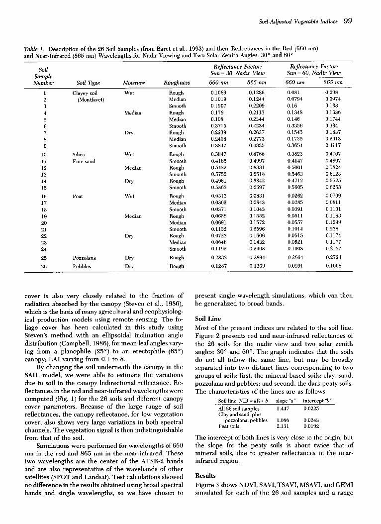
Table 1. Description of the 26 Soil Samples (from Baret et al., 1993) and their Reflectances in the Red (660 nm) and Near-Infrared (865 nm) Wavelengths for Nadir Viewing and Two Solar Zenith Angles: 30 ° and 60 °

Soil Reflectance Factor: Reflectance Factor: Sample Sun = 30, Nadir View Sun = 60, Nadir View

Number Soil Type Moisture Roughness 660 nm 865 nm 660 nm 865 nm

1 Clayey soil Wet Rough 0.1069 0.1286 0.081 0.098 2 (Montfavet) Median 0.1019 0.1244 0.0794 0.0974 3 Smooth 0.1907 0.2209 0.16 0.188 4 Median Rough 0.176 0.2113 0.1348 0.1636 5 Median 0.198 0.2344 0.146 0.1744 6 Smooth 0.3715 0.4234 0.3356 0.384 7 Dry Rough 0.2239 0.2637 0.1545 0.1837 8 Median 0.2408 0.2773 0.1735 0.2013 9 Smooth 0.3847 0.4335 0.3654 0.4117

10 Silica Wet Rough 0.3847 0.4766 0.3823 0.4707 11 Fine sand Smooth 0.4185 0.4997 0.4147 0.4897 12 Median Rough 0.5422 0.6331 0.5001 0.5824 13 Smooth 0.5752 0.6518 0.5463 0.6123 14 Dry Rough 0.4961 0.5842 0.4712 0.5525 15 Smooth 0.5863 0.6597 0.5605 0.6263

16 Peat Wet Rough 0.0313 0.0831 0.0262 0.0709 17 Median 0.0302 0.0843 0.0285 0.0811 18 Smooth 0.0371 0.1043 0.0391 0.1101 19 Median Rough 0.0686 0.1552 0.0511 0.1183 20 Median 0.0691 0.1572 0.0557 0.1299 21 Smooth 0.1132 0.2596 0.1014 0.238 22 Dry Rough 0.0723 0.1606 0.0515 0.1174 23 Median 0.0646 0.1432 0.0521 0.1177 24 Smooth 0.1192 0.2468 0.1008 0.2167

25 Pozzolana Dry Rough 0.2832 0.2894 0.2664 0.2724

26 Pebbles Dry Rough 0.1287 0.1309 0.0991 0.1008

cover is also very closely related to the fraction of radiation absorbed by the canopy (Steven et al., 1986), which is the basis of many agricultural and ecophysiolog- ical p roduc t ion models using remote sensing. The foliage cover has been calculated in this study using Steven's me thod with an ellipsoidal inclination angle distribution (Campbell, 1986), for mean leaf angles varying from a planophile (25 °) to an erectophi le (65 °) canopy; LAI varying f rom 0.1 to 8.

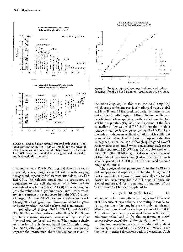
By changing the soil undernea th the canopy in the SAIL model , we were able to est imate the variations due to soil in the canopy bidirectional reflectance. Re- flectances in the red and near-infrared wavelengths were c o m p u t e d (Fig. 1) for the 26 soils and different canopy cover parameters . Because of the large range of soil reflectances, the canopy reflectance, for low vegetat ion cover, also shows very large variations in both spectral channels. The vegetat ion signal is then indistinguishable from that of the soil.

Simulations were per formed for wavelengths of 660 nm in the red and 865 nm in the near-infrared. These two wavelengths are the cen te r of the ATSR-2 bands and are also representat ive of the wavebands of other satellites (SPOT and Landsat). Test calculations showed no difference in the results obtained using broad spectral bands and single wavelengths, so we have chosen to

present single wavelength simulations, which can then be general ized to broad bands.

Soil Line Most of the present indices are related to the soil line. Figure 2 presents red and near-infrared reflectances of the 26 soils for the nadir view and two solar zenith angles: 30 ° and 60 ° . The graph indicates that the soils do not all follow the same line, but may be broadly separated into two distinct lines cor responding to two groups of soils: first, the mineral-based soils: clay, sand, pozzolana and pebbles; and second, the dark peaty soils. The characteristics of the lines are as follows:

Soil line: NIR = aR + b slope "a" intercept "b" All 26 soil samples 1.447 0.0225 Clay and sand, plus

pozzolona, pebbles 1.086 0.0243 Peat soils 2.131 0.0192

The intercept of both lines is very close to the origin, but the slope for the peaty soils is about twice that of mineral soils, due to greater reflectances in the near- infrared region.

Results Figure 3 shows NDVI, SAVI, TSAVI, MSAVI, and GEMI simulated for each of the 26 soil samples and a range

1 0 0 Rondeaux et al.

0506 I L A ¢ T M . .

0 4

0 3 e~

" - -

01

0 I

0 I

0 8 LAI= 0.1

0 7

0 6 I l l l

0 5

0 4

~ o 3

0 2

O I

0 I I l l

R e d R e f l e c t a n c e s (660 n m ) ; 26 s o i l s

S o l a r z e n i t h a n g l e = 30 ° ; V i e w = 0 °

Ellip~oidal leaf angle distribution

LAI= 0.5

65 ° Leaf Angle(°)

J 55 ° • [q 45 ° LAI= 1

- L~ 35° o / • - D 25 o

• • 55 ° • ½ 4 5 ° \ ~ , . o

I I I I I

O2 03 04 05 0 6

cover

LAI=2

L A I = 4 & 8

{I 7 0 g 0 9 l

N e a r - I n f r a r e d R e f l e c t a n c e s (865 n m ) ; 26 s o i l s

S o l a r z e n i t h a n g l e = 3 0 ° ; V i e w = 0 °

LAI= 4 & 8 LAI = 0.5 LAI= I LAI= 2

65° Leaf Angle (°)

I I I I I I I I I

O2 0 3 0 4 1) 5 I) 6 0 7 O8 O9 I

cover

Figure 1. Red and near-infrared spectral reflectances simulated with the SAIL + SOILSPECT model for the range of 26 soil samples, as a function of foliage cover (0 = bare soil; 1 = 100% cover) represented by a range of leaf area index and leaf angle distributions.

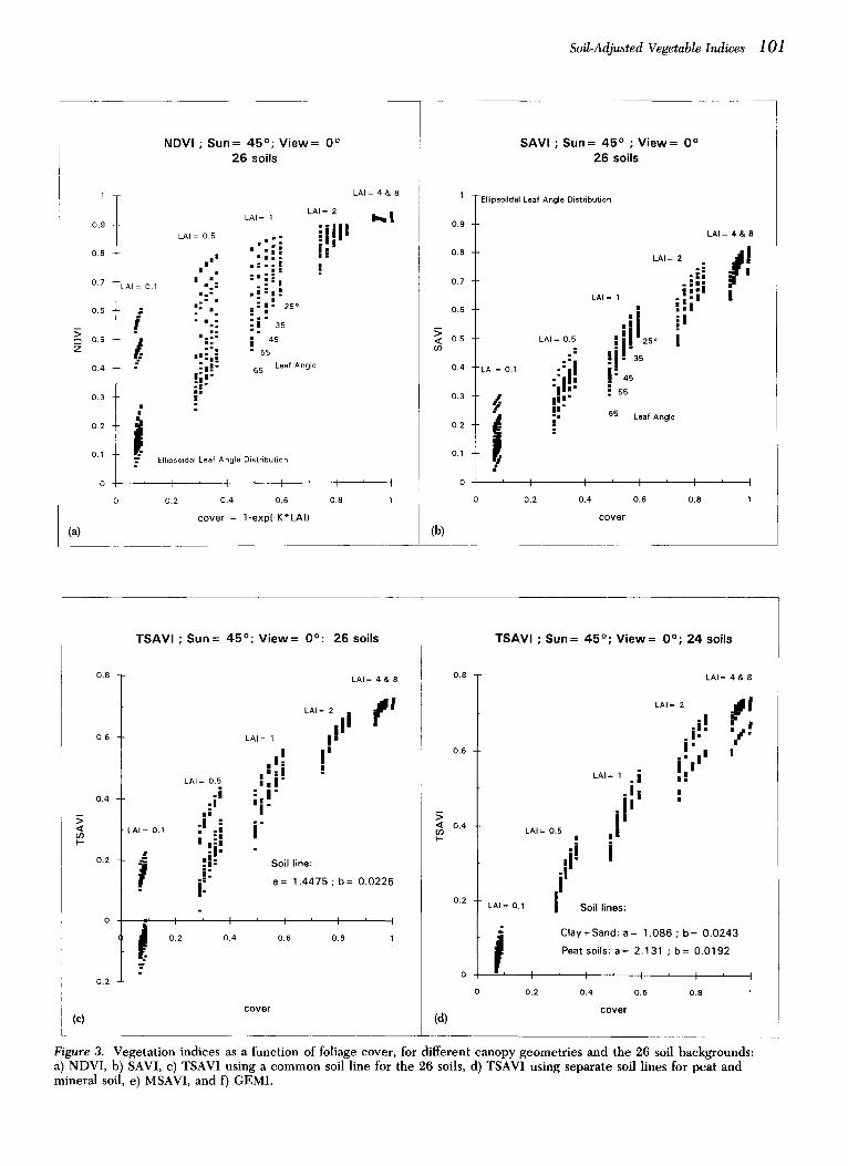
of canopy covers. The NDVI (Fig. 3a) demonstrates, as expected, a very large range of values with varying background, especially for low vegetation densities. For LAI~< 0.1, the reflected signal may be considered as equivalent to the soil signature. With intermediate amounts of vegetation (0.5 < LAI < 3) the wide range of possible values could produce very large errors when trying to retrieve the plant cover from the NDVI values. At large LAI, the NDVI reaches a saturation level. Clearly NDVI will give poor information about a vegetation canopy when the soil background is unknown.

Soil-adjusted indices, SAVI, TSAVI, and MSAVI (Fig. 3b, 3c, and 3e), perform better than NDVI. Some problems remain, however, because of the use of a universal soil line for all soil types. When using a single soil line for all soils (averaging all the 26 single lines), the TSAVI, although better than NDVI, does not greatly improve the information about the vegetation given by

Soi l Ref l ec tances of 26 soi l samples : N a d i r v i ew ; S u n zen i th ang les= 30 & 60 °

05

O4

03

o 2

/

/

/ /

I I o I o 2

f / '

f

/

/

/

[ I O3 O4

Red Reflectance

t , !

t~ Qa}

• Sand

• Peat

Pozzolona

Pebbles

Soil line

Soil iinc peat

I [

Figure 2. Relationships between near-infrared and red reflectances for the 26 soil samples, resulting in two soil lines.

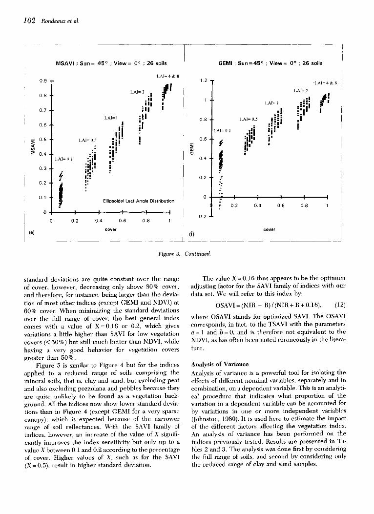
the index (Fig. 3c). In this case, the SAVI (Fig. 3b), which uses coefficients previously adjusted from a global soil line (Huete, 1988), produces a slightly better result, but still with quite large variations. Better results may be obtained when applying coefficients from the two soil lines separately (Fig. 3d): the dispersion of the data is smaller at low values of LAI, but here the problem reappears at the larger cover values (LAI >2) where the index produces an artificial variation, with a different value of saturation level for each group of soils. This divergence is not realistic, although quite good overall performance is obtained when considering each group of soils separately. MSAVI (Fig. 3e) is quite similar to SAVI (Fig. 3b). GEMI (Fig. 3f) displays a wide spread of the data at very low cover (LAI = 0.1), then a much smaller spread for LAI >i 0.5, but also a reduced dynamic range of the index.

The choice of the parameter L in the SAVI-type indices appears to be quite critical in minimizing the soil background effect. Figure 4 shows normalized standard deviations, accounting for the full range of soils, for several indices and for the general formulation of the "SAVI family" of indices, simplified to:

VI = (NIR - R) / (NIR + R + X) (11)

where we prefer to note the adjusting factor "X" instead of"L" because of its variability. The multiplication factor (1 + L) has been left out, because it only significantly affects the index at relatively large values of L (> 0.4). All indices have been normalized between 0 (for the minimum value) and 1 (for the maximum at 100% cover) before calculation of the standard deviation.

For low vegetation cover, if no information about the soil type is available, then SAVI and MSAVI have the lowest standard deviations with soil variation. Their


1

0.9

0.8

0.7

0.6

tm 0.5 Z

0 .4

0.3

0.2

0.1

0

LAI = 0.1

i /.

t

N D V I ; S u n = 4 5 ° ; V i e w = 0 ° 2 6 s o i l s

LAI= I

LAI = 05

":i • g l i

I II Ill- m==.. =

I , .==."

I • : a iD= I

• : - • ,= =! . " : . . . . : : ' 250

:: :!" 3~ i . . • 45

l = I

==m = 55 , , : , : . I Leaf Angle

| =

LAI = 2

j!ll' LAI = 4 & 8

Ellipsoidal Leaf Angle Distribution

I I ' I I ' I

0.2 0 .4 0.6 0.8 1

c o v e r = 1 - e x p ( - K * L A I )

S A V I ; S u n = 4 5 ° ; V i e w = 0 ° 2 6 s o i l s

1

0.9

0.8

0.7 -

0.6 -

0.5 -

0.4 - LAI = 0.1

0.3 - .ff~

0.2 - ~

0.1 - I #

0

-Ellipsoildal Leaf Angle Distribution

LAI = 1

LAI = 0.5

. :

.;iJ! | ! "

| | "

i"

LAI = 2

'ii!2 ° ! i - I ' • 45

: 55

LAI = 4 & 8

! . i : a

. ii i , | = l

i I I

65 Leaf Angle

I I ' I I I

0.2 0 .4 0.6 0.8 1

c o v e r

(a) (b)

m

(c)

T S A V I ; S u n = 4 5 ° ; V i e w = 0 ° : 2 6 s o i l s

0.8

0 .6

0 .4

0.2

-0.2

LAI = 0.5

.i .! | I

_AI = o.1 ;= |

i ,:. l

i-

LAI = I

I = 1 1,1"

~i! I

LAI = 4 & 8

LA;,,, r i I

!

So i l l i ne :

a = 1 . 4 4 7 5 ; b = 0 . 0 2 2 5

-' l I ' I ' I ' I

t ! 0.2 0 .4 0.6 0.8 1

c o v e r

0.8

0.6

0.4

(d)

0.2

T S A V I ; S u n = 4 5 ° ; V i e w = 0 ° ; 2 4 s o i l s

L A I = 0.5

L A I = 0.1

L A I = 4 & 8

L A I = 1 . i

,i i',' !

.li! i ,I | Soil lines:

LAI = 2

. i ! !

!i;" I I

Clay+Sand: a= 1 .086 ; b= 0 .0243

Peat soils: a = 2 . 1 3 1 ; b = 0 .0192

I I I I I

0.2 0.4 0.6 0 .8 1

cover

Figure 3. Vegetation indices as a function of foliage cover, for different canopy geometries and the 26 soil backgrounds: a) NDVI, b) SAVI, c) TSAVI using a common soil line for the 26 soils, d) TSAVI using separate soil lines for peat and mineral soil, e) MSAVI, and f) GEMI.

1 0 2 Rondeaux et al.

0.9

0.8

0.7

0.6

.~ 0.5 <

0.4

0.3

0.2

0.1

0

(e)

M S A V I ; S u n = 4 5 ° ; V i e w = 0 ° ; 2 6 soi ls

LAI= 0.5

LAI= Ol "::|i!

.,. ..;!i'. - n;;

Nan "

I I 0.2 0.4

LAI=, !

!! ! i o i

LAI=4&8

LA,:2. t I n i l m

i l l n

:iN !u ! ,

Ellipsoidal Leaf Angle Distribution

I I I

0.6 0.8 1

c o v e r

1.2

0.8

0.6

L9 0.4

0.2

0

-0.2 t

(f)

GENI I ; S u n = 4 5 ° ; V i e w = 0 ° ; 2 6 soi ls

LAI= 0. l

t ::

°

I • 0.2

LAI= 1

| ; m LAI =0.5 !|.roll'" "

"" :i"'

1 '

"LAI= 4 & 8

LAI= 2

I ! I I 0.4 0.6 0.8 1

c o v e r

Figure 3. Continued.

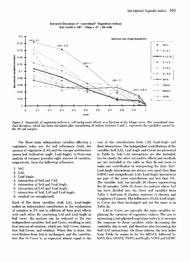
standard deviations are quite constant over the range of cover, however, decreasing only above 80% cover, and therefore, for instance, being larger than the deviation of most other indices (except GEMI and NDVI) at 60% cover. When minimizing the standard deviations over the full range of cover, the best general index comes with a value of X=0 .16 or 0.2, which gives variations a little higher than SAVI for low vegetation covers (< 50%) but still much better than NDVI, while having a very good behavior for vegetation covers greater than 50%.

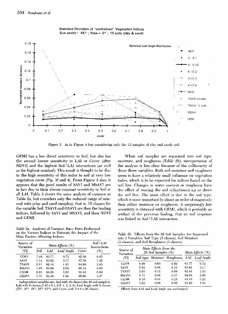
Figure 5 is similar to Figure 4 but for the indices applied to a reduced range of soils comprising the mineral soils, that is, clay and sand, but excluding peat and also excluding pozzolana and pebbles because they are quite unlikely to be found as a vegetation background. All the indices now show lower standard deviations than in Figure 4 (except GEMI for a very sparse canopy), which is expected because of the narrower range of soil reflectances. With the SAVI family of indices, however, an increase of the value of X significantly improves the index sensitivity but only up to a value X between 0.1 and 0.2 according to the percentage of cover. Higher values of X, such as for the SAVI (X = 0.5), result in higher standard deviation.

The value X = 0.16 thus appears to be the optimum adjusting factor for the SAVI family of indices with our data set. We will refer to this index by:

OSAVI = (NIR - R) / (NIR+ R+0.16), (12)

where OSAVI stands for optimized SAVI. The OSAVI corresponds, in fact, to the TSAVI with the parameters a = 1 and b = 0, and is therefore not equivalent to the NDVI, as has often been noted erroneously in the litera- ture.

A n a l y s i s o f V a r i a n c e

Analysis of variance is a powerful tool for isolating the effects of different nominal variables, separately and in combination, on a dependent variable. This is an analyti- cal procedure that indicates what proportion of the variation in a dependent variable can be accounted for by variations in one or more independent variables (Johnston, 1980). It is used here to estimate the impact of the different factors affecting the vegetation index. An analysis of variance has been performed on the indices previously tested. Results are presented in Ta- bles 2 and 3. The analysis was done first by considering the full range of soils, and second by considering only the reduced range of clay and sand samples.

Soil-Adjusted Vegetable Indices 1 0 3

S t a n d a r d D e v i a t i o n o f " n o r m a l i z e d " V e g e t a t i o n I n d i c e s

S u n z e n i t h = 4 5 ° ; V i e w = 0 ° ; 2 6 soi ls

0.2

0 .18

0 .16

o 0 . 1 4

"o 0 .12

~ 0.1

0 .08

E 0 .06

z

0 .04

0.02

LAI = 0.1 Spherical Leaf Angle Distribution

~ LAI= 0.5

0 x " ' ' -

" ~ ' - ~ " - " -x " ' ' ' - " ~ ~ ">~q~ - - - - - -

, , , , , , , ,- 0.1 0.2 0 .3 0.4 0.5 0 .6 0.7 0.8 0,9 1

cover

- A - - X = 0 . 2

- - × - - X = 0 . 3

- - x - - - X = O . 4

• SAVI

- e - - TSAVI

- - + MSAVI

-<3- - GEMI

Figure 4. Sensitivity of vegetation indices to soil background effects, as a function of the foliage cover. The normalized standard deviation, which has been calculated after normalizing all indices between 0 and 1, represents the variability caused by the 26 soil samples.

The three main independent variables affecting a vegetation index are: the soil reflectance (Soil), the amount of vegetation (LAI) and the canopy architecture (mean leaf inclination angle: Leaf-Angle). A three-way analysis of variance provides eight sources of variation, respectively, from the following influences:

1. Soil, 2. LAI, 3. Leaf-Angle, 4. interaction of Soil and LAI, 5. interaction of Soil and Leaf-Angle, 6. interaction of LAI and Leaf-Angle, 7. interaction of Soil, LAI and Leaf-Angle, 8. residual (or unexplained).

Each of the three variables (Soil, LAI, Leaf-Angle) makes an independent contribution to the explanation of variation in VI, and in addition all have joint effects with each other. By combining LAI and Leaf-Angle as leaf cover, the analysis can be reduced to the two independent variables: Soil and Cover, resulting in only four sources of variation, which are: Soil, Cover, interaction Soil-Cover, and residual. When this is done, the contribution from Soil is unchanged, and the contribution due to Cover is, as expected, almost equal to the

sum of the contributions from LAI, Leaf-Angle and their interactions. The independent contributions of the variables Soil, LAI, Leaf-Angle and Cover are presented in Table 2a. Soil/LAI interactions are also included, but for clarity the other interactive effects and residuals are not included in the table as they do not seem to make any contribution to interpreting the data: Soil/ Leaf-Angle interactions are always very small (less than 0.05%) and unsignificant; LAI / Leaf-Angle interactions are part of the cover contribution and less than 1%. The variable, Soil, has initially 26 classes representing the 26 samples. Table 2b shows the analysis where Soil has been divided into the three soil variables from Table 1: Soil-type (5 classes), moisture (3 classes), and roughness (3 classes). The influences of LAI, Leaf-Angle, or Cover are then unchanged and are the same as in Table 2a.

LAI or Cover are naturally the main variables ex- plaining the variation of vegetation indices. The aim in optimizing a soil-adjusted vegetation index is to increase the response to these variables while decreasing the variability due to soil, and therefore also decreasing the Soil/LAI interactions. On these criteria, the best index from Table 2a seems to be the MSAVI, followed by SAVI, then OSAVI, TSAVI and finally NDVI and GEMI.

104 Rondeaux et al.

S t a n d a r d Devia t ion of "normal ized" V e g e t a t i o n Indices Sun z e n i t h = 4 5 ° ; V i e w = 0 ° ; 15 soils (c lay & sand)

o =

g$

E

Z

0 .18

0 .16

0 .14

0.12

0.1

0 .08

0 .06

0.04

0.02

0

Spherical Leaf Angle Distribution

\

\ \\\

\ \\\

\\\

' \

I I I I I ) I I I "~ ,h ~ 0.1 0.2 0.3 0.4 0,5 0.6 0.7 0.8 0.9 1

cover

41 NDVI

*- X - 0 . 1

• X = 0 . 1 6

• X - 0 . 2

- - x X = 0 . 3

- ~( X = 0 . 4

• SAVI

o TSAVI all soils

- <> TSAVI 15 soils

• MSAVI

• GEMI i

Figure 5. As in Figure 4 but considering only the 15 samples of clay and sandy soil.

GEMI has a low direct sensitivity to Soil, but also has the second lowest sensitivity to LAI or Cover (after NDVI) and the highest Soil/LAI interactions (as well as the highest residual). This result is thought to be due to the high sensitivity of this index to soil at very low vegetation cover (Fig. 3f and 4). From Figure 4 also, it appears that the good results of SAVI and MSAVI are in fact due to their almost constant sensitivity to Soil at all LAI. Table 3 shows the same analysis of variance as Table 2a, but considers only the reduced range of mineral soils (clay and sand samples), that is, 15 classes for the variable Soil. TSAVI and OSAVI are then the leading indices, followed by SAVI and MSAVI, and then NDVI and GEMI.

Table 2a. Analyses of Variance Have Been Performed on the Various Indices to Estimate the Impact of the Main Factors Affecting Indices

Source of Soil/LAI Variation Main Effects (%) Interactions

(VI) Soil LAI Leaf Angle Cover (%)

NDVI 7.49 83.77 0.73 85.36 6.93 SAVI 1.14 93.92 3.17 97.59 1.22 TSAVI 2.11 92.44 1.83 94.90 2.93 MSAVI 1.05 94.68 2.60 98.18 0.69 CEMI 0.93 88.28 3.22 91.94 6.99 OSAVI 1.71 93.40 1.94 95.98 2.27

Independent variables are: Soil with 26 classes (the 26 soil samples), LAI with 6 classes (LAI = 0.1, 0.5, 1, 2, 4, 8), Leaf Angle with 5 classes (25 °, 35 °, 45 °, 55 °, 65°), and Cover with 5 x 6 = 30 classes.

When soil samples are separated into soil type, moisture, and roughness (Table 2b), interpretation of the analysis is less clear because of the collinearity of these three variables. Both soil moisture and roughness seem to have a relatively small influence on vegetation index, which is to be expected for indices based on the soil line. Changes in water content or roughness have the effect of moving the soil reflectances up or down the soil line. The main effect is due to the soil type, which is more important by about an order of magnitude then either moisture or roughness. A surprisingly low sensitivity is obtained with GEMI, which is probably an artifact of the previous finding, that its soil response was linked to Soil/LAI interaction.

Table 2b. Effects from the 26 Soil Samples Are Separated into 3 Variables: Soil Type (5 classes), Soil Moisture (3 classes), and Soil Roughness (3 classes)

Source of Variation

Wt)

Main Effects front the 26 Soil Samples (%) Main Effects (%)

Soil type Moisture Roughness LAI Leaf Angle

NDVI 6.89 0.60 0.59 83.77 0.73 SAVI 0.83 0.08 0.35 93.92 3.17 TSAVI 2.03 0.12 0.09 92.44 1.83 MSAVI 0.71 0.08 0.37 94.68 2.60 GEM1 0.10 0.04 0.19 88.28 3.22 OSAVI 1.63 0.09 0.08 93.40 1.94

Effects from LAI and Leaf Angle are unchanged.


Table 3. Same as Table 2a, But Considering only 15 Classes for the Variable Soil: 15 Clay and Sand Samples

Source of Main Effects (%) Soil/LAI Variation Interactions

(VI) Soil LAI Leaf Angle Cover (%)

NDVI 0.97 96.33 0.89 98.19 0.78 SAVI 0.99 95.37 2.79 98.62 0.34 TSAVI 0.10 97.31 1.79 99.76 0.10 MSAVI 1.04 95.54 2.23 98.57 0.31 GEMI 0.57 89.66 2.57 92.52 6.78 OSAVI 0.06 97.37 1.74 99.76 0.15

DISCUSSION

The soil background is a major surface component con- trolling the spectral behavior of vegetation canopies, and on which the retrieval of biophysical characteristics of the canopy depends. The sensitivity of different vegetation indices to soil color has been investigated. Al- though vegetation indices, such as the soil-adjusted vegetation indices, considerably reduce these soils effects, estimation of the vegetation characteristics from the indices still suffers from some imprecision, especially at relatively low cover, if no information about the target is known.

The first problem was the use of the soil line, which cannot be generalized because of its variability. Even though the 26 soil samples from Table 1 represent a very large range of spectral values, a question still re- mains about their' representativity. The anomalous soil line encountered with the peaty soil has been investigated further. The peat soil used for the simulation was taken from a bag of commercial peat compost (Baret, personal communication) and is assumed to have a high organic-matter content. A small experiment was conducted to test the differentiation between peat and mineral soil lines seen in Figure 2. Spectral signatures of an independent set of soil samples were measured with a high resolution spectroradiometer (Rondeaux, 1995). Soil samples were collected in agricultural fields in East Anglia, UK, including light-brown soils and soils designated as peat on British Soil Survey maps. An organic potting soil from a commercial bag was also tested. The results are shown in Figure 6, where all soils taken from fields, including the peaty soils, follow the same line with a slope of 1.35, whereas the bagged soil shows a line with a much higher slope of about 3.5. Although the absolute values of these slopes are somewhat greater than those in Figure 2, this result seems to confirm the assumption that the second soil line observed in Figures 2 and 6 is due to the high organic content of the soil (Stoner et al., 1980, NcNairn and Protz, 1993). The peat (as in Table 1) or highly organic composts from commercial bags, are not very representative of peat soils found in the real world,

60

50

4O

m-

-~ 30 =

2O

10

dry peaty soils

• we t peaty soi ls

• we t soi ls

dry soi ls

soi l l ine

po t t ing soil I

2nd soi l l ine

z

"' I I I 5 10 15

Red Reflectance

I 2O

Figure 6. Relationships between near-infrared and red reflectances of different soil samples measured with the Sin- gle-FOV-IRIS spectroradiometer (Rondeaux, 1995).

although they are a good addition to a data set to test and validate models.

In the general formulation of the "SAVI family" of indices, the minimization of the soil effect is done by adjustment of the parameter X. In this study, the value of X has been reexamined to optimize the index sensitivity with our soil data set. The value X=0.16 is found to give satisfactory reduction of soil noise, both at low and high vegetation cover. The resulting index, OSAVI, is attractive because of its simple formulation: It is a simplified version of the TSAVI, which does not require any preliminary knowledge of the soil line parameters. This index is currently being applied semi-operationally for sugar beet yield prediction and management in the UK (Xu and Steven, 1995).

The main objectives of vegetation remote sensing are to analyze, interpret, and monitor temporal vegetation changes on seasonal or annual time scales, The optimal choice of a vegetation index is still very much related to the purpose of study and the type of vegetation considered as well as to the amount of prior information available. In agricultural studies over a single soil type there is a little to choose between the indices studied here, but for the generalization and intercomparison of results from different places, it is desirable to standard- ize on a single, soil-invariant index. No generalization can easily be made, however. Simulations have been done here by means of the SAIL model, which charac- terizes homogeneous canopies such as grass and agricultural crops at mid-latitudes. TSAVI or OSAVI seem to

106 Rondeaux et al.

offer the best results for this kind of canopy. In arid climates where the vegetation cover is generally less than 25%, MSAVI may be bet ter (Fig. 5), whereas both SAVI and MSAVI, which have a slightly higher but more constant sensitivity over the full range of cover, could also be quite useful for general-purpose vegetation classification. To make progress, we suggest, for the reasons outlined above, that OSAVI should be adopted for agricultural applications, whereas MSAVI is r ecommended for more general purposes. Standardization of vegetation indices is important at this stage of progress of the science and further empirical evaluation of indices is required to establish confidence in any standards to be adopted.

This work is part of a research project on "Biophysical Indices, from ATSR-2 ~ supported by a grant from the UK Natural Environment Research Council (NERC). The authors gratefully acknowledge the anonymous referees for their helpful comments.

REFERENCES

Baret, F., and Guyot, G. (1991), Potentials and limits of vegetation indices for LAI and PAR assessment, Remote Sens. Environ. 35:161-173.

Baret, F., Jacquemoud, S., and Hanocq, J. F. (1993), The soil line concept in remote sensing, Remote Sens. Rev. 7:65- 82.

Bausch, W. C. (1993), Soil background effects on reflectance- based crop coefficients for corn, Remote Sens. Environ. 46: 213-222.

Campbell, G. S. (1986), Extinction coefficients for radiation in plant canopies calculated using an ellipsoidal inclination angle distribution. Agric. For. Meteorol. 36:317-321.

Cierniewski, J., and Courault, D. (1993), Bidirectional reflectance of bare soil surfaces in the visible and near-infrared range, Remote Sens. Rev. 7:321-339.

Clevers, J. G. P. W., and Verhoef, W. (1993), LAI estimation by means of the WDVI: A sensitivity analysis with a combined PROSPECT-SAIL model, Remote Sens. Environ. 7:43-64.

Curran, P. J., Foody, G. M., and Kondratyev, K. Ya., Kozod- erov, V. V., and Fedchenko, P. P. (1990), Remote Sensing of Soils and Vegetation in the USSR, Taylor & Francis.

Escadafal, R. (1993), Remote sensing of soil colour: Principles and applications. Remote Sens. Rev. 7:261-279.

Escadafal, R., and Huete A. (1991), Etude des propr6t6s spectrales des sols arides appliqude h l'am61ioration des indices de vdg6tation obtenus par t616ddtection, C. R. Acad. Sci. Paris, 312:1385-1391.

Huete, A. R. (1988), A soil-adjusted vegetation index (SAVI), Remote Sens. Environ. 25:295-309.

Irons, J. R., Weismiller, R. A., and Petersen, G. W. (1989), Soil reflectance, in Theory and Application of Optical Remote Sensing, (G. Asrar, Ed.), Wiley Interscience, New York, pp. 66-106.

Jacquemoud, S., Baret, F., and Hanocqu, J. F. (1992), Model- ling spectral and bidirectional soil reflectance, Remote Sens. Environ. 41:123-132.

Jasinki, M. F., and Eagleson, P. S. (1989), The structure of red-infrared scattergrams of semivegetated landscapes, IEEE Trans. Geosci. Remote Sens. 27:441-451-.

Johnston, R. J. (1980), Multivariate Statistical Analysis in Geog- raphy, Longman Scientific & Technical, in press.

Kaufman, Y. J., and Tanr6 D. (1992), Atmospherically resistant vegetation index (ARVI) for EOS-MODIs, IEEE Trans. Geosci. Remote Sens. 30 (2):261-270.

Kuusk, A. (1991), The hot-spot effect in plant canopy reflectance, in Photon-Vegetation Interactions, Application in Op- tical Remote Sensing and Plant Ecology. (Myneni and Ross, Eds.), Springer Velag, New York, pp. 139-159.

McNairn, H., and Protz R. (1993), Mapping corn residue cover on agricultural fields in Oxford county, Ontario, using Thematic Mapper, Can. Remote Sens. 19:152-159.

Malthus, T. J. (1989), Anglo-French Collaborative Reflectance Experiment. Experiement 1, Brooms Barn Station, July 1989. Internal report, University of Nottingham.

Myneni, R. B., and Asrar G. (1994), Atmospheric effects and spectral vegetation indices, Remote Sens. Environ. 47:390- 402.

Pinty, B., and Verstraete, M. M. (1992), GEMI: A non-linear index to monitor global vegetation from satellites, Vegeta- tion 101:15-20.

Qi, J., Huete, A. R., Moran, M. S., Chehbouni, A., and Jackson, R. D. (1993), Interpretation of vegetation indices derived from multi-temporal SPOT images, Remote Sens. Environ. 44:89-101.

Qi, J., Chehbouni, AI., Huete, A. R., Kerr, Y. H., and Soroos- hian, S. (1994), A modified soil adjusted vegetation index (MSAVI) Remote Sens. Environ. 48:119-126.

Rondeaux, G. (1995), Analysis of Soil Spectral Properties with the GER Single Field-of-View IRIS, Internal report, Geog- raphy Department, University of Nottingham, Nottingham, UK.

Sellers, P. J., Berry, J. A., Collatz, G. J., Field, C. B., and Hall, F. G. (1992), Canopy reflectance, photosynthesis and transpiration III. A reanalysis using improved leaf models and a new canopy integration scheme, Remote Sens. Envi- ron. 42:187-216.

Soil Survey Staff (1975), Soil taxonomy: A Basic System of Soil Classification for Making and Interpreting Soil Survey, Soil Conservation Office. U.S. Dept. of Agric. Handbook, no. 436. Washington, D.C.

Steven, M. D., Biscoe, P. V., Jaggard, K. W., and Paruntu J. (1986), Foliage cover and radiation interception, Field Crops Res. 13:75-87.

Steven, M. D., Malthus, T. J., Danson, F. M., Jaggard, K. W., and Andrieu, B. (1992), Monitoring Response of Vegetation to Stress, in Proceedings Remote Sensing Society Annual Conference, Dundee, UK. Remote Sensing from Research to Operation, pp. 369-377.

Steven, M. D., Malthus, T. J., and Baret, F. (1994), Intercali- bration of vegetation indices from different sensor systems, In 6th International Symposium Physical Measurements and Signatures in Remote Sensing. Val D'Isere, France, January 94 (In press).

Stoner, E. R., Baumgardner, M. F., Biehl, L. L., Robinson, B. F. (1980), Atlas of soil reflectance properties. Research Bulletin 962, Laboratory for Application of Remote Sensing, Purdue University, West Lafayette, Indiana, 75 pp.


Verhoef, W. (1984), Light scattering by leaf layers with application to canopy reflectance modelling: the SAIL model, Remote Sens. Environ. 16:125-141.

Xia, Li. (1994), A two-axis vegetation index (TWVI), Int. J. Remote Sens. 15:1447-1458.

Xu, H., and Steven, M. D. (1995), Intercalibration of airborne and satellite optical systems. Sugar beet prediction and management. Technical note no. SBP-UN-TN-008. Univer- sity of Nottingham and Logica UK.

Optimization of soil-adjusted vegetation indices

Documents