Optimization of redundant degree of freedom in robot milling ...

Optimization of redundant degree of freedom inrobot milling considering chatter stabilityYu Liu  ( [email protected] )

Northeastern UniversityLinwei Wang 

Northeastern UniversityYe Yu 

Northeastern UniversityJinyu Zhang 

Northeastern UniversityBin Shu 

Northeastern University

Research Article

Keywords: robotic milling, redundant degree of freedom, optimization method , chatter stability

Posted Date: February 17th, 2022

DOI: https://doi.org/10.21203/rs.3.rs-1360661/v1

License: This work is licensed under a Creative Commons Attribution 4.0 International License.  Read Full License

Manuscript Title

Optimization of redundant degree of freedom in robot milling considering

chatter stability

Author names:

Linwei Wang, Yu Liu *, Ye Yu , Jinyu Zhang, Bin Shu

Author email addresses:

Linwei Wang, E-mail: [email protected];

Corresponding author: Yu Liu, E-mail: [email protected], Tel: 0086-13072498580;

Ye Yu, E-mail: [email protected];

Jinyu Zhang ,E-mail:[email protected]

Bin Shu , E-mail:[email protected]

Affiliation address:

School of Mechanical Engineering & Automation, Northeastern University, Shenyang 110819, China;

Abstract：

Aiming at the redundant degree of freedom problem of six axis industrial robot performing five axis milling task, a

new optimization method of robot milling redundant degrees of freedom considering chatter stability was proposed.

Taking the limit cutting depth of robot milling regenerative chatter as the optimization objective, and combined

with the constraints of robot motion performance (avoiding joint limit, singular pose and collision), a redundant

degree of freedom optimization model considering chatter stability was established. The milling experimental

results showed that the new optimization method of robot milling redundant degrees of freedom considering

chatter stability proposed in this paper can effectively avoid robot milling regenerative chatter and improve

machining quality and efficiency.

Keywords: robotic milling, redundant degree of freedom, optimization method , chatter stability

Acknowledgements

Funding: This research was supported by National Natural Science Foundation of China (No. 51875094).

Conflicts of interest/Competing interests: The authors declare that there is no conflict of interest

regarding the content of this article.

Ethics approval (Not applicable)

Consent to participate (Consent)

Consent for publication (Consent)

Availability of data and material :All data generated or analysed during this study are included in

this published article.

Code availability (Not applicable)

Authors' contributions: Linwei Wang: Conceptualization, Methodology, Software, Validation,

Formal analysis, Investigation, Data curation, Writing original draft, Visualization. Yu Liu:

Resources, Supervision, Funding acquisition. Ye Yu , Jinyu Zhang , and Bin Shu: Software,

Investigation, Writing - review & editing

Highlights:

1. A new optimization method of redundant degrees of freedom in robotic milling considering chatter stability is

proposed to determine the optimal redundant degrees of freedom when a six axis industrial robot performs a five

axis milling task.

2. Experiments verify the feasibility of this method to avoid robotic milling regenerative chatter and improve

machining quality and efficiency, It provides a theoretical basis for the setting of redundant degrees of freedom in

robotic machining CAM system.

3. The optimal redundancy degree of freedom significantly improves the chatter stability of robot high-speed

milling.

Optimization of redundant degree of freedom in robot milling considering

chatter stability

Linwei Wang, Yu Liu *, Ye Yu

(School of Mechanical Engineering & Automation, Northeastern University, Shenyang 110819, China. Corresponding author: Yu Liu, E-mail: [email protected])

Abstract：

Aiming at the redundant degree of freedom problem of six axis industrial robot performing five axis milling task, a

new optimization method of robot milling redundant degrees of freedom considering chatter stability was proposed.

Taking the limit cutting depth of robot milling regenerative chatter as the optimization objective, and combined

with the constraints of robot motion performance (avoiding joint limit, singular pose and collision), a redundant

degree of freedom optimization model considering chatter stability was established. The milling experimental

results showed that the new optimization method of robot milling redundant degrees of freedom considering

chatter stability proposed in this paper can effectively avoid robot milling regenerative chatter and improve

machining quality and efficiency.

Keywords: robotic milling, redundant degree of freedom, optimization method , chatter stability

1 Introduction

With the advantages of large working space, high flexibility and low cost, industrial robots have been

gradually applied in the field of milling, such as the processing of automobile inspection tools, ship hulls and large

aircraft parts [1]. However, the development of CAM systems for robot machining is far behind that for machine

tool machining.

In recent years, some mainstream commercial off-line programming software such as RobotStudio and

KUKA-Sim have successively launched robot machining modules, which can convert the G code generated by

five-axis milling modules in CAD/CAM software into robot program, realizing automatic programming of

complex parts machining[2]. Series industrial robots used for milling usually have 6 degrees of freedom, while the

tool point pose information in G code only contains position X, Y, Z and orientation A and B. Therefore, the

six-axis industrial robot performing five-axis milling tasks will lead to one redundant degree of freedom, namely

the degree of freedom rotating around the axis of the tool[3]. At present, the commercial off-line programming

software needs to be manually set by users to complete the transformation of robot program. However, there is a

lack of theoretical basis for setting and optimizing the redundant degrees of freedom.

The optimization of redundant degrees of freedom in robot machining has become an important research

content in recent years. Scholars have put forward different optimization objectives, such as joint limit, flexibility,

Cartesian stiffness and so on. Zhu et al.[4]proposed the joint limit performance index and took it as the

optimization objective to make each joint axis of the robot away from the joint limit angle through the optimal

selection of redundant degrees of freedom. Zargarbashi et al.[5]took Jacobian condition number as the

optimization objective of flexibility, aiming to make better use of redundant degrees of freedom to avoid robot

singularity. In order to improve the robot milling accuracy, Chen et al.[6] took the normal stiffness as the

optimization objective and the joint limit as the constraint condition to optimize the redundant degrees of freedom

and feed direction. In order to improve the production efficiency of robot milling, Xiong et al.[7] took the feed

direction stiffness as the optimization objective and the joint limit and singularity as the constraints to optimize the

redundant degrees of freedom of the five axis milling industrial robot. Lu et al.[8] proposed a joint motion

planning algorithm based on redundant degree of freedom optimization to realize smooth and collision free

machining. Xiao [9]established a multi-objective optimization model of joint limit, flexibility and collision to

determine the redundant degrees of freedom of a six-axis industrial robot in five-axis milling applications.

Aiming at the optimization of redundant degrees of freedom in robot machining, the optimization objectives

proposed in the existing literature mainly focus on improving the kinematics of the robot, avoiding collision and

improving the Cartesian stiffness of the robot end effector, ignoring the chatter stability of robot machining.

However, some researchers[10-12] found through experimental research that regenerative chatter is the main

reason for the instability of robot high-speed milling process. Chatter will not only affect the machining quality,

reduce the tool life, and even damage the robot. Celikag et al.[13] also confirmed the view that regenerative chatter

plays a dominant role in robot milling from two aspects of theoretical analysis and experimental research. Mejri et

al.[14]found through experimental modal analysis that the change of robot pose will cause the dynamic change of

tool tip, and then affect the stability of machining process. On this basis, Mousavi et al.[15-18] studied the

influence of redundant degrees of freedom on milling stability based on the robot dynamics model. The results

show that the transition from unstable zone to stable zone can be realized by controlling redundant degrees of

freedom without modifying cutting parameters. Therefore, it is very necessary to consider the chatter stability

when setting the redundant degrees of freedom in the robot machining CAM system. However, the optimization of

redundant degrees of freedom with the ultimate cutting depth of robot milling regenerative chatter as the

optimization objective has not been published.

Taking the limit cutting depth of regenerative chatter in robot milling as the optimization objective and the

motion performance of the robot as the constraint condition, this paper establishes an optimization model of

redundant degrees of freedom in robot milling considering chatter stability, which provides a theoretical basis for

the setting of redundant degrees of freedom in robot machining cam system. The feasibility and effectiveness of

the model are verified by milling experiments.

2 Problem description of redundant degrees of freedom in robot milling

A serial robot has redundant degrees of freedom when the operational space dimension (n) is larger than the

degree t of the task performed(t). The redundant degrees of freedom(rn) is determined as follows

nr n t (1)

geometric modeling

tool path planning

coordinate transformation

G code(x,y,z,A,B)

(x,y,z,α,β) remove redundancy

code conversion

reverse the Euler angle

(x,y,z,α,β,γ)

Robot program

Machining simulation

Milling robot

CAD/CAM

CAM Converter

User-Setγ

CL(x,y,z,i,j,k)

Optimized robot program

Off-line programming simulation platform

Optimization process

Regenerative Chatter limit cut depth

Joint limit

flexibilityNo

collision

objective

constraint conditions

(a)traditional method (b)new method

geometric modeling

tool path planning

coordinate transformation

G code(x,y,z,A,B)

(x,y,z,α,β) remove redundancy

code conversion

reverse the Euler angle

(x,y,z,α,β,γ)

Robot program

Machining simulation

Milling robot

CAD/CAM

CL(x,y,z,i,j,k)

Optimized robot program

γ

Joint limit

flexibility

stiffness

Fig.1 Comparison of pose optimization methods

Fig.1(a) shows the process of G code conversion robot program in the robot machining module of commercial

off-line programming software.

First, generate G code: use CAD/CAM software for geometric modeling, tool path planning and generate G

code.

Then, reverse the Euler angle: the cutter location CL(x, y, z, i, j, k) data described in the workpiece coordinate

system can be obtained from the G code, where (x, y, z) is the coordinate of the tool tip point and (i, j, k) is the unit

vector of the tool axis direction. The pose of the robot tool coordinate system T relative to the workpiece

coordinate system W is represented by a six-dimensional vector (x, y, z, α, β, γ), where(α, β, γ) is a Z-Y-Z Euler

angle.The homogeneous transformation matrix of the tool coordinate system relative to the workpiece coordinate

system is

= ( , , ) ( , ) ( , ) ( , )W

Tx y z z y z T trans rot rot rot (2)

Where, trans and rot are translation matrix and rotation matrix respectively.

Therefore, when the robot executes the robot program converted by G code for milling, the tool position data

and matrix must meet the following requirements: Therefore, when executing the robot program converted by G

code for milling, the cutter location data and matrix W

TT have to satisfy :

0 0

0 0

1 0

0 1 0 1

W

T

i z

j y

k x

T (3)

It can be deduced from equation (3) that

T Tcos sin sin sin cosi j k (4)

From equation (4), it can be seen that for a given CL(x, y, z, i, j, k), only the former five components of the

six-dimensional vector (x, y, z, α, β, γ)can be determined, while the Euler angle γ is arbitrary. Therefore, when a

six-axis industrial robot performs a five-axis milling task, a redundant degree of freedom will be generated, which

is quantified by the Euler angle γ.

Thirdly, remove redundancy: the Euler angle γ needs to be set when solving the robot inverse kinematics, that

is, the process of removing redundancy. This value should be given by the optimization process.

Finally, conversion code: the transformed robot program is processed and simulated, and the executable

optimized robot program is output.

3 Redundant degree of freedom optimization model considering chatter stability

As shown in Fig.1, the traditional method takes joint limit, flexibility and Cartesian stiffness as the

optimization objectives to determine the redundant degrees of freedom γ， However, the chatter stability of robotic

machining has not been considered. Therefore, a new redundant degree of freedom optimization method

considering chatter stability is proposed in this paper.

The optimal redundant degree of freedom γ is determined by maximizing the limit cutting depth aplim(γ) of

the regenerative chatter in the robotic milling to avoid the occurrence of regenerative chatter. In addition, it is

necessary to avoid the joint angles of the robot from approaching the limit position, being in singular pose and

collision. The redundant degree of freedom optimization model considering chatter stability was established

plim

1min max

( )

( )

, 1

max

. . | |

,( ) ,, 2 ,6j

a b

j

K J

a

s t T L r

j

r

f

L

＞

(5)

Where aplim(γ) is the regeneration chatter limit cutting depth; K(J) is the reciprocal of the conditional number of the

normalized Jacobian matrix of the robot; η is a user-defined flexibility value. T is the distance between two

bounding boxes; L is the detection axis; ra and rb are the projections of radius of bounding boxes A and B on the

detection axis; θi is the joint angle of the robot; f -1() represents inverse kinematics; and θmin and θmax are joint

limits.

4 Solution of redundant degree of freedom optimization model

4.1 The limit cutting depth of the regenerative chatter in the robotic milling

4.1.1 Dynamic model of robot milling system

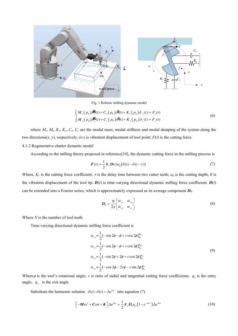
As shown in Fig.2, the dynamic model of the robot milling system can be simplified into a 2-DOF vibration

system in the x-axis and y-axis directions. For a given configuration p0 in Cartesian space, the dynamic model of

the tool tip can be expressed by equation (6):

workspace

X

Z

Kx x

yz

Ky

x

y

Fr

Cy

Kx

Ky

n

Ft

f

Cx

F

Y

Fig. 1 Robotic milling dynamic model

0 0 0

0 0 0

( ) ( ) ( ) ( )

( ) ( ) ( ) ( )

x x x x y x

y y y y y y

M p t C p t K p t F t

M p t C p t K p t F t

&& &

&& &

(6)

where Mx, My, Kx, Ky, Cx, Cy are the modal mass, modal stiffness and modal damping of the system along the

two directions(x, y), respectively. ( )t is vibration displacement of tool point; F(t) is the cutting force.

4.1.2 Regenerative chatter dynamic model

According to the milling theory proposed in reference[19], the dynamic cutting force in the milling process is

p

1( ) ( ) [ ( ) ( )]

2ct K t a t t F D (7)

Where, Kc is the cutting force coefficient; 𝜏 is the delay time between two cutter teeth; ap is the cutting depth; 𝛿 is

the vibration displacement of the tool tip. D(t) is time-varying directional dynamic milling force coefficient. D(t)

can be extended into a Fourier series, which is approximately expressed as its average component D0.

0

2

xx xy

yx yy

N

D (8)

Where N is the number of tool teeth.

Time-varying directional dynamic milling force coefficient is

1= [ sin 2 cos 2 ]

2

1= [ sin 2 cos 2 ]

2

1= [ sin 2 2 cos 2 ]

2

1= [ cos 2 2 sin 2 ]

2

ex

st

ex

st

ex

st

ex

st

yx

yx

xy

xx

r

r

r

r r

(9)

Where is the tool’s rotational angle; r is ratio of radial and tangential cutting force coefficients; st is the entry

angle; ex is the exit angle.

Substitute the harmonic solution ( ) : ( ) Δ i tt t e

into equation (7)

20 p

1Δ a 1 Δ2

i t i i t

ci e K e e

M C K D (10)

4.1.3 The limit cutting depth of the regenerative chatter

The frequency response function of the tool tip is

12( ) i

H M C K (11)

By substituting the frequency response function into equation (10)

0 p

1a 1 ( ) Δ 0

2i

cK e

I D H (12)

If the determinant below is zero, then equation (12) has a nontrivial solution.

0 p

1det a 1 ( ) 0

2i

cK e

I D H (13)

Since the frequency response function is complex, the characteristic equation (13) has real and imaginary

parts, and the eigenvalue at chatter frequency is given by

p= 14

+ a ci

cR

Nei K

(14)

It can be obtained by solving equation (14)

cos sinci

c ce i (15)

p

Λ 1 cos Λ sin Λ 1 cos Λ sin2

1 cos 1 cos

R c I c I c R c

c c c

a iNK

(16)

Where the imaginary part of ap must be equal to zero because ap is a real number.

The real part of a p gives the limit cutting depth (aplim) in chatter frequency (ωc), which separates the stable

and instable zone. If κ is defined as

sinΛΛ 1 cos

cI

R c

(17)

Therefore, limit cutting depth of the regenerative chatter (aplim) can be written as

2plim

t

2 Λ1Ra

NK

(18)

4.1.4 The influence of redundant degree of freedom γ on the limit cutting depth aplim(γ)

As shown in Fig.3, it is a block diagram of the regenerative chatter in the robotic milling. It can be seen from

the figure that the change of the robot's pose will cause the dynamic changes of the tool tip point, which will affect

the stability of the processing. Therefore, for each robot pose with the same cutting parameters, the limit cutting

depth aplim(γ) is determined according to equation (18), aplim(γ) is a function of the redundant degree of freedom

γ.

4.2 The robotic flexibility index

The condition number of the normalized Jacobian matrix of the robot is used to measure the closeness of the

robot to the singularity[20], which is expressed as

-1( )=cond( )=C J J J J (19)

Where J is Jacobian matrix, ( ) [1, )C J .

The robotic flexibility index is expressed as

( )=1/ ( )K CJ J (19)

The closer the K(J) value is to 1, the better the flexibility. The K(J) value is close to 0, indicating that the joint

angle of the robot at this time is close to the singularity position.

Kcap H(ω)=[-M(pi)ω2+iC(pi)ω+K(pi)]

-1

delay time:τ

+ +

-+

h(t) F(t)

inner modulation:δ(t)

outer modulation:δ(t-τ)

h0(t)

Redundancy γi

Joint angle θj=f -1(γi)

M(pi) C(pi) K(pi)

inverse kinematics-Joint angle θj

forward kinematics-pose pi

Fig.3 Regenerative chatter block diagram in robotic machining

4.3 Robot collision free condition

A B

OAOB

L

L ra rb

T

Fig. 4 OBB bounding box detection pump

The OBB bounding box intersection detection is used to determine whether there is a collision between the

detected robot link and the detected object[21]. To test whether the bounding boxes intersect, it is necessary to

project the center and radius of the bounding boxes onto the detection axis L. If the distance between the centers of

the bounding boxes on the axis is greater than the sum of the radius, the bounding boxes are separated. T is the

distance between two bounding boxes, L is the detection axis which is one of the 15 separation axes, ai and bi are

half the side lengths of bounding boxes A and B, respectively, and Ai and Bi as the side direction vectors of

bounding boxes A and B, ra and rb are the projections of radius of bounding boxes A and B on the detection axis,as

shown in Figure 4.

The detection axis and the projections of the radius of the bounding box on the detection axis are respectively

1,2,3

1,2,3

1,2,3 1,2,3

i

j

i j

A i

L B j

A B i j

(21)

11

3 3,

ji

a i i b j jr a A L r b B L

(22)

The projection distance between the center points of the boxes is |T·L|, so the condition that the bounding

boxes do not intersect is if and only if

| |a b

T L r r (23)

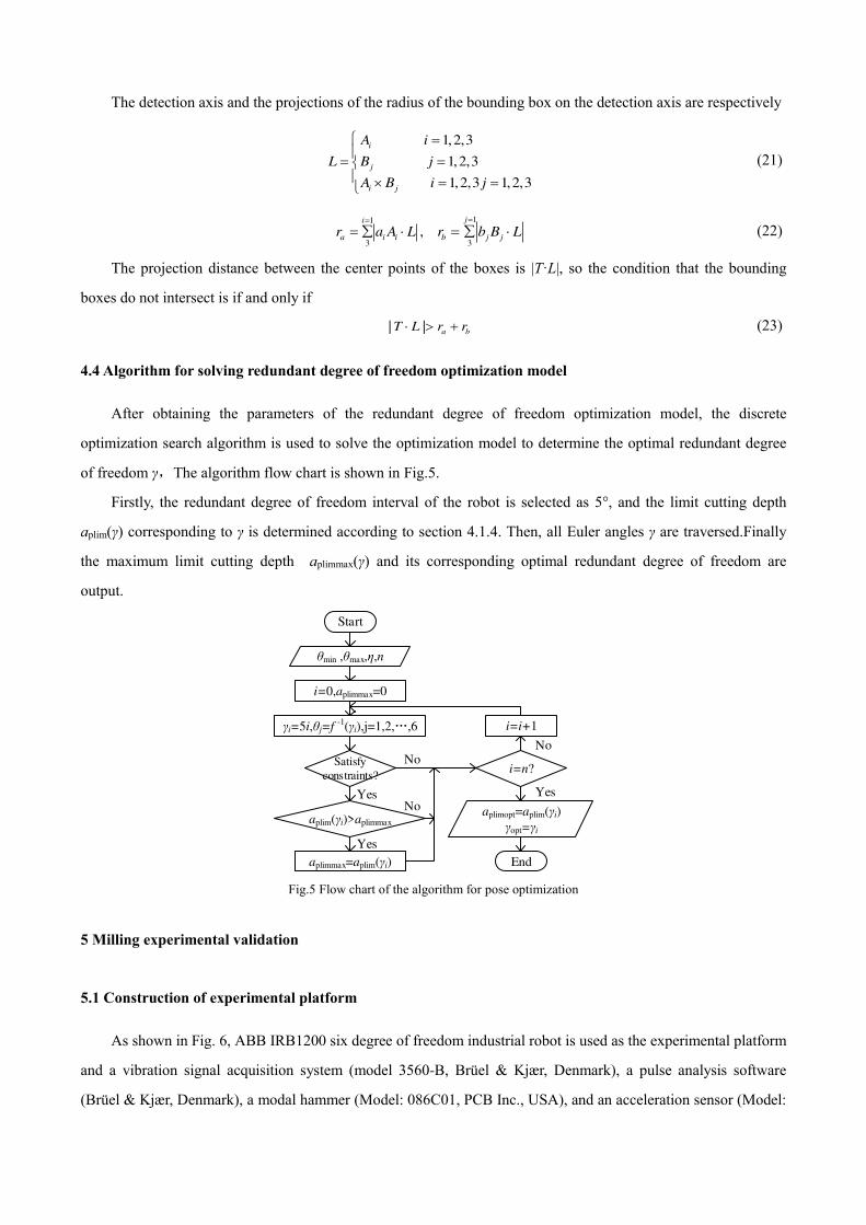
4.4 Algorithm for solving redundant degree of freedom optimization model

After obtaining the parameters of the redundant degree of freedom optimization model, the discrete

optimization search algorithm is used to solve the optimization model to determine the optimal redundant degree

of freedom γ，The algorithm flow chart is shown in Fig.5.

Firstly, the redundant degree of freedom interval of the robot is selected as 5°, and the limit cutting depth

aplim(γ) corresponding to γ is determined according to section 4.1.4. Then, all Euler angles γ are traversed.Finally

the maximum limit cutting depth aplimmax(γ) and its corresponding optimal redundant degree of freedom are

output.

Start

θmin ,θmax,η,n

i=0,aplimmax=0

γi=5i,θj=f -1(γi),j=1,2, ,6

Satisfy constraints?

aplim(γi)>aplimmax

aplimmax=aplim(γi)

i=n?

i=i+1

aplimopt=aplim(γi)γopt=γi

End

No

Yes

Yes

Yes

No

No

Fig.5 Flow chart of the algorithm for pose optimization

5 Milling experimental validation

5.1 Construction of experimental platform

As shown in Fig. 6, ABB IRB1200 six degree of freedom industrial robot is used as the experimental platform

and a vibration signal acquisition system (model 3560-B, Brüel & Kjær, Denmark), a pulse analysis software

(Brüel & Kjær, Denmark), a modal hammer (Model: 086C01, PCB Inc., USA), and an acceleration sensor (Model:

356A24, PCB Inc., USA) were used for data collection from the milling system.

Pulse

3560B

356A24

ABB IRB1200

086C01

Fig.6 the experimental platform for robotic milling

5.2 Construction of simulation platform RobotYY

Robotyy is an off-line programming simulation software for six axis industrial robot milling developed by the

author on python, QT and OpenGL platforms.It mainly has modules such as off-line programming post-processing,

machining simulation and collision detection. The software interface is shown in Fig.7.

Fig.7 Software interface

The post-processor interface is shown in Fig.8. G code (NC format) is converted into robot program through

post-processing algorithms such as motion instruction conversion, coordinate calculation and posture calculation.

In addition, the post-processing module can also predict FRF of other estimated pose according to the imported

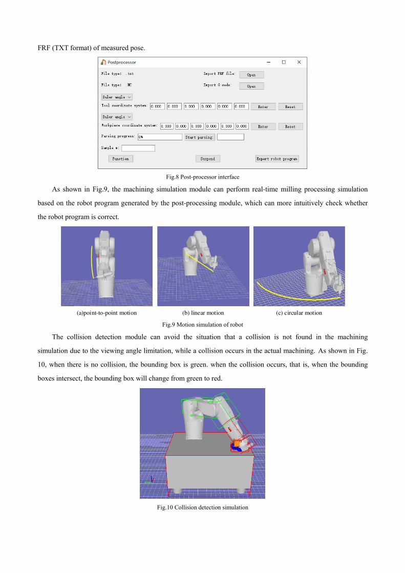
FRF (TXT format) of measured pose.

Fig.8 Post-processor interface

As shown in Fig.9, the machining simulation module can perform real-time milling processing simulation

based on the robot program generated by the post-processing module, which can more intuitively check whether

the robot program is correct.

(a)point-to-point motion (b) linear motion (c) circular motion

Fig.9 Motion simulation of robot

The collision detection module can avoid the situation that a collision is not found in the machining

simulation due to the viewing angle limitation, while a collision occurs in the actual machining. As shown in Fig.

10, when there is no collision, the bounding box is green. when the collision occurs, that is, when the bounding

boxes intersect, the bounding box will change from green to red.

Fig.10 Collision detection simulation

5.3 Experimental verification of redundant degrees of freedom optimization

5.3.1 Prediction of frequency response function

In recent years, two methods have been used to predict the frequency response function of the tool tip of the

robot: (1)Data modeling based on experiment[22-24]; (2)Theoretical modeling based on finite element method[17].

Due to the complexity of the robot structure, material properties, transmission system layout, etc., it is difficult to

establish an accurate and reliable theoretical model to describe the dynamic characteristics of the robot tool tip. In

practical applications, the modal hammering experiment is usually used to obtain the frequency response function

of the robot tool tip, and the experimental results are more reliable. Note that there are an infinite number of robot

poses in the robot workspace. It is very time-consuming to obtain the frequency response function of the tool tip

point in each robot pose through experiments. Therefore, this paper uses the frequency response function of the

measured poses to accurately and efficiently predict the frequency response function of other estimated poses,

based on the inverse distance weighting method. This method is simple and efficient, and has good interpolation

effect for uniformly distributed sample points[24].

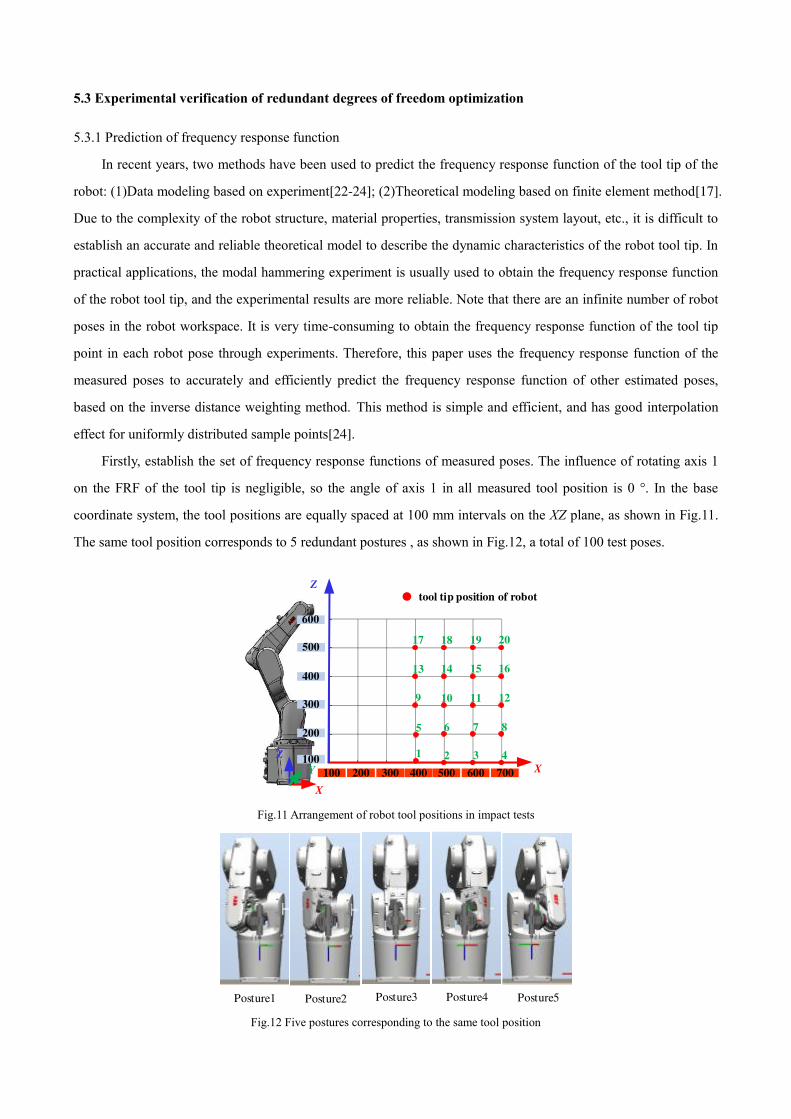
Firstly, establish the set of frequency response functions of measured poses. The influence of rotating axis 1

on the FRF of the tool tip is negligible, so the angle of axis 1 in all measured tool position is 0 °. In the base

coordinate system, the tool positions are equally spaced at 100 mm intervals on the XZ plane, as shown in Fig.11.

The same tool position corresponds to 5 redundant postures , as shown in Fig.12, a total of 100 test poses.

100

500

400

300

200

100

200 300 700600500400

tool tip position of robot

X

Z

17

13

9

18

14

10

6

2

19

15

11

7

3

20

16

12

8

4Z

X

Y

1

5

600

Fig.11 Arrangement of robot tool positions in impact tests

Posture1 Posture2 Posture3 Posture4 Posture5

Fig.12 Five postures corresponding to the same tool position

Then, determine the number of samples m. Since the influence of the measured pose FRF on the estimated

pose decreases with the increase of distance di, the measured pose is sorted according to distance di, and the

frequency response function of the nearest m measured poses is selected to predict the frequency response function

of the estimated pose. In this paper, M is determined as 10.

2 2 21 1 2 2 6 6= ( ) ( ) ( )

i j i j i j id q q q q q q L (24)

Where di is the Euclidean distance between the estimated pose(qj) and the measured pose(qi) in the joint space.

After that, the weight λi of each test point is calculated. The weight λi is a function of the reciprocal of the

distance, and satisfies the following relationship:

1

=1m

i

i (25)

1

1

1i

i m

i i

d

d

(26)

Finally, predict the frequency response function. The frequency response function Hj(ω) of any estimated

pose in the robot workspace can be predicted based on the frequency response function Hi(ω) of the m measured

poses, which is determined by

1

( ) ( )m

j i i

i

H H (27)

150 200 250 300 350 400frequency (Hz)

-4

-2

0

2

4

10-6

measured

identified

150 200 250 300 350 400

-6

-4

-2

0

10-6

150 200 250 300 350 400-1

-0.5

0

0.5

1

10-5

150 200 250 300 350 400-1.5

-1

-0.5

0

10-5

(a)x direction (b)y direction

Rea

l(m

/N)

Rea

l(m

/N)

Imag(m

/N)

Imag

(m/N

)

measured

identified

measured

identified

measured

identified

frequency (Hz)

frequency (Hz) frequency (Hz)

Fig.13 Frequency response function of robot tool tip

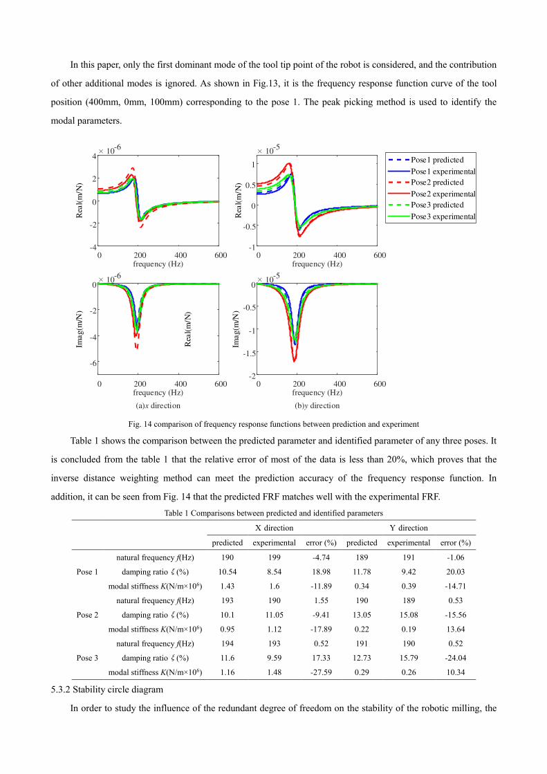
In this paper, only the first dominant mode of the tool tip point of the robot is considered, and the contribution

of other additional modes is ignored. As shown in Fig.13, it is the frequency response function curve of the tool

position (400mm, 0mm, 100mm) corresponding to the pose 1. The peak picking method is used to identify the

modal parameters.

0 200 400 600-4

-2

0

2

4

10-6

0 200 400 600

-6

-4

-2

0

10-6

0 200 400 600-1

-0.5

0

0.5

1

10-5

0 200 400 600-2

-1.5

-1

-0.5

0

10-5

Rea

l(m

/N)

Rea

l(m

/N)

Rea

l(m

/N)

Imag

(m/N

)

Imag

(m/N

)

frequency (Hz)

frequency (Hz)

frequency (Hz)

frequency (Hz)

(a)x direction (b)y direction

Pose1 predicted

Pose1 experimental

Pose2 predicted

Pose2 experimental

Pose3 predicted

Pose3 experimental

Fig. 14 comparison of frequency response functions between prediction and experiment

Table 1 shows the comparison between the predicted parameter and identified parameter of any three poses. It

is concluded from the table 1 that the relative error of most of the data is less than 20%, which proves that the

inverse distance weighting method can meet the prediction accuracy of the frequency response function. In

addition, it can be seen from Fig. 14 that the predicted FRF matches well with the experimental FRF. Table 1 Comparisons between predicted and identified parameters

X direction Y direction

predicted experimental error (%) predicted experimental error (%)

Pose 1

natural frequency f(Hz) 190 199 -4.74 189 191 -1.06

damping ratioξ(%) 10.54 8.54 18.98 11.78 9.42 20.03

modal stiffness K(N/m×106) 1.43 1.6 -11.89 0.34 0.39 -14.71

Pose 2

natural frequency f(Hz) 193 190 1.55 190 189 0.53

damping ratioξ(%) 10.1 11.05 -9.41 13.05 15.08 -15.56

modal stiffness K(N/m×106) 0.95 1.12 -17.89 0.22 0.19 13.64

Pose 3

natural frequency f(Hz) 194 193 0.52 191 190 0.52

damping ratioξ(%) 11.6 9.59 17.33 12.73 15.79 -24.04

modal stiffness K(N/m×106) 1.16 1.48 -27.59 0.29 0.26 10.34

5.3.2 Stability circle diagram

In order to study the influence of the redundant degree of freedom on the stability of the robotic milling, the

position of the tool tip point remains unchanged, and the redundant degree of freedom γ is changed, that is, it

rotates around the z-axis of the tool coordinate system. At each change of 5°, the frequency response function of

tool point was predicted, and a total of 38 groups of frequency response curves were predicted. The peak picking

method was used to identify modal parameters, drawing the stability lobe diagram, as shown in Fig.15.

2000

1504000

6000 1008000

10000 50

2

12000014000

4

6

aplim

(mm

)

Fig.15 Stable lobe diagram

In Fig.15, the limit cutting depth of the same spindle speed (12000 RPM as an example) and its corresponding

redundant degrees of freedom were taken to draw the circle diagram aplim(γ), as shown in Fig.16.The radius of the

circle represents the limit cutting depth , and the radian of the circle represents the redundant degree of freedom.

The discrete optimization search algorithm in Section 4.4 is used to solve the redundant degree of freedom

optimization model equation (5) to determine the optimal redundant degree of freedom γopt=115°, and the

maximum limit cutting depth aplimmax=1.345mm.

0.5

1

1.5

30

210

60

240

90

270

120

300

150

330

180 0

0.5

1

γ/(°)

instable zone

stable zone

unreachable zone

max

(115，1.345)

min

(0，0.579)

Fig.16 Stability circle diagram

5.3.3 Experimental verification

In order to verify the influence of redundant degrees of freedom on the milling stability of the robot, the

6061-T6 aluminum alloy machining experiment is carried out with ABB IRB1200 robot under the optimal

redundant degrees of freedom of 115° and redundant degrees of freedom of 0 °, as shown in Fig.17. The Cutting

parameters in experimental machining are shown in Table 2.

(a)γ=115° (b)γ=0° Fig.17 Experiment machining of robot milling

Table 2 Cutting parameters in experimental machining

redundancy Spindle speed Feed rate Depth of cut predicted experimental

115° 12000rpm 1mm / s 1mm stable stable

0° 12000rpm 1mm / s 1mm instable instable

Fig. 18(a) shows the acceleration signal spectrum at the optimal redundant degree of freedom of 115 °, and

the frequencies 201 Hz and 402 Hz are the rotating frequency and cutter tooth passing frequency respectively. In

Fig. 18 (b), in addition to the rotating frequency and cutter tooth passing frequency, there is also a peak value of

341 Hz, which is not the cutter tooth passing frequency or its harmonic, but the regenerative chatter frequency. The

experimental results are consistent with the predicted results, as shown in Table 2.

5

10

20

0

15

0 100 200 300 400 500

rotating frequency 201Hz

frequency/Hz

acce

lera

tion

/(m

/s2 )

Tooth passing frequency 402Hz

20

15

10

5

25

30

0 100 200 300 400 500

rotating frequency201Hz

Chatter frequency 341Hz

frequency/Hz

acce

lera

tion/

(m/s

2 )

Tooth passing frequency 402Hz

0

(a)γ=115° (b)γ=0°

Fig. 18 Spectrum diagram of acceleration signal

Another indicator to measure the stability of robot milling is the surface quality of the machining parts. When chatter occurs, obvious chatter marks will be left on the surface of parts. As shown in Fig.19, the surface quality of the optimal redundant degree of freedom of 115° (Ra=2.5μm)is significantly better than that of the redundant degree of freedom of 0°(Ra=9.2μm), which also shows that the stability of the optimal redundant degree of freedom 115 ° is significantly better than that of the redundant degree of freedom 0 °.

γ=0°(Ra=9.2μm)

γ=115°(Ra=2.5μm)

Fig.19 Surface comparison of parts machined

6. Conclusions

(1) A new optimization method of redundant degrees of freedom in robotic milling considering chatter

stability is proposed to determine the optimal redundant degrees of freedom when a six axis industrial robot

performs a five axis milling task. Experiments verify the feasibility of this method to avoid robotic milling

regenerative chatter and improve machining quality and efficiency, It provides a theoretical basis for the setting of

redundant degrees of freedom in robotic machining CAM system.

(2) The maximum limit cutting depth of 1.345mm corresponding to the optimal redundancy degree of

freedom (115°) is 1.323 times higher than the minimum limit cutting depth of 0.579mm corresponding to the

redundancy degree of freedom (0°), which significantly improves the chatter stability of robot high-speed milling.

Acknowledgements

This research was supported by National Natural Science Foundation of China (No. 51875094).

References:

[1]Zhu Z , Tang X , Chen C et al(2021) High precision and efficiency robotic milling of complex parts:

Challenges, approaches and trends. Chinese Journal of Aeronautics (5).https://doi.org/10.1016/j.cja.2020.12.030

[2]Pan Z , J Polden, N Larkin, et al(2012) Recent progress on programming methods for industrial robots. Robot

Comput Integrat Manufact 28(2)87-94. https://doi.org/10.1016/j.rcim.2011.08.004

[3]Xiong G , Ding Y , Zhu L M (2019) Stiffness-based pose optimization of an industrial robot for five-axis

milling. Robot Comput Integrat Manufact 55 19-28. https://doi.org/10.1016/j.rcim.2018.07.001

[4]W.Zhu, et al., An off-line programming system for robotic drilling in aerospace manufacturing. Int J Adv

Manufact Technol 68(9-12) (2013) 2535-2545. DOI:10.1007/s00170-013-4873-5

[5]Zargarbashi S , Khan W , Angeles J (2012)The Jacobian condition number as a dexterity index in 6R

machining robots. Robot Comput Integrat Manufact 28(6) :694-699.

https://doi.org/10.1016/j.rcim.2012.04.004

[6]Chen C , Peng F , Yan R et al (2019)Stiffness performance index based posture and feed orientation

optimization in robotic milling process.Robot Comput Integrated Manufact 55: 29–40.

https://doi.org/10.1016/j.rcim.2018.07.003

[7] Xiong G , Ding Y , Zhu L M et al(2017) A Feed-Direction Stiffness Based Trajectory Optimization Method

for a Milling Robot. International Conference on Intelligent Robotics and Applications (C).

DOI:10.1007/978-3-319-65292-4_17

[8] Lu Y A , Tang K , Wang C Y (2021)Collision-free and smooth joint motion planning for six-axis industrial

robots by redundancy optimization. Robot Comput Integrated Manufact 68:102091.

https://doi.org/10.1016/j.rcim.2020.102091

[9]Xiao W , Huan J (2012)Redundancy and optimization of a 6R robot for five-axis milling applications:

singularity, joint limits and collision. Production Engineering 6(3): 287-296.

DOI:10.1007/s11740-012-0362-1

[10]Hao D , Wang W , Liu Z et al(2020)Experimental study of stability prediction for high-speed robotic milling

of aluminum. Journal of Vibration and Control 26(7-8) :387-398.DOI:10.1177/1077546319880376

[11]Cordes M , Hintze W , Altintas Y (2019) Chatter stability in robotic milling.Robot Comput Integrat Manufact

55 : 11–18. https://doi.org/10.1016/j.rcim.2018.07.004

[12]LIU Y and Feng-xia H(2019) Research on the Influencing Factors of Robot Milling Stability. Journal of

Northeastern University(Natural Science) 40(07):991-996. [in Chinese]

DOI:10.12068/j.issn.1005-3026.2019.07.015

[13]Celikag H , Ozturk E , Sims N D (2021) Can mode coupling chatter happen in milling? Int J Mach Tools

Manuf 165: 103738. https://doi.org/10.1016/j.ijmachtools.2021.103738

[14]Mejri S ,Gagnol V,et al (2016)Dynamic characterization of machining robot and stability analysis. Int J Adv

Manufact Technol82 (1-4) :351–359.

DOI:10.1007/s00170-015-7336-3

[15]Mousavi S G , Gagnol V , Bouzgarrou B C et al(2018) Stability optimization in robotic milling through the

control of functional redundancies. Robot Comput Integrated Manufact 50 (Supplement C):181–192.

https://doi.org/10.1016/j.rcim.2017.09.004

[16]Mousavi S G , Gagnol V , Bouzgarrou B C et al(2017)Control of a Multi Degrees Functional Redundancies

Robotic Cell for Optimization of the Machining Stability. Procedia CIRP 58 :269-274.

https://doi.org/10.1016/j.procir.2017.04.004

[17]Mousavi S G , Gagnol V , Bouzgarrou B C et al(2017) Dynamic modeling and stability prediction in robotic

machining, Int. J. Adv Manufact Technol88 (9):3053–3065.

[18]Mousavi S G , Gagnol V , Bouzgarrou B C et al(2013)Dynamic Behavior Model Of A Machining

Robot and Stability Prediction. ECCOMAS, Zagreb.

[19]Altinta Y , Budak E(1995) Analytical Prediction of Stability Lobes in Milling. CIRP Annals 44(1) :357-362.

https://doi.org/10.1016/S0007-8506(07)62342-7

[20]Khan W A , Angeles J (2006) The Kinetostatic Optimization of Robotic Manipulators: The Inverse and the

Direct Problems. Journal of Mechanical Design 128(1): 168-178.DOI:10.1115/1.2120808

[21]Fan Q , Gong Z , Tao B , et al (2021) Base position optimization of mobile manipulators for machining large

complex components. Robot Comput Integrated Manufact 70(5-8) :102138.

https://doi.org/10.1016/j.rcim.2021.102138

[22]Nguyen V , Melkote S(2021)Hybrid statistical modelling of the frequency response function of industrial

robots. Robot Comput Integrated Manufact 70:102134.

https://doi.org/10.1016/j.rcim.2021.102134

[23]Nguyen V , Cvitanic T , Melkote S Melkote(2019)Data-driven modeling of the modal properties of a 6-dof

industrial robot and its application to robotic milling. Journal of Manufacturing Science and Engineering

141(12):1-24.

DOI:10.1115/1.4045175

[24]Chen C , Peng F , Yan R et al (2018) Posture-dependent stability prediction of a milling industrial robot based

on inverse distance weighted method. Proc Manuf 17: 993–1000.

https://doi.org/10.1016/j.promfg.2018.10.104