NATIONAL UNIVERSITY OF SINGAPORE Department of Physics Optimization of Practical Covert Communication Author: Ignatius William Primaatmaja Supervisor: Prof. Valerio Scarani Mentor: Dr. Juan Miguel Arrazola A thesis submitted in partial fulfillment of the requirements for the degree of Bachelor of Science (Hons) April 2017

Welcome message from author
This document is posted to help you gain knowledge. Please leave a comment to let me know what you think about it! Share it to your friends and learn new things together.
Transcript

NATIONAL UNIVERSITY OF SINGAPORE
Department of Physics
Optimization of Practical Covert
Communication
Author:
Ignatius William
Primaatmaja
Supervisor:
Prof. Valerio Scarani
Mentor:
Dr. Juan Miguel Arrazola
A thesis submitted in partial fulfillment of the requirements for the degree of
Bachelor of Science (Hons)
April 2017


Abstract
Covert communication allows two parties to communicate with low probability of
detection by the adversaries. As a trade-off, it usually takes a long time to send
a message covertly. In this report, we consider the covert communication scheme
proposed in Ref. [2] and perform an optimization over protocol parameters in order
to significantly reduce the number of channel uses and the time required to transmit
a classical message of fixed length. We propose a model in which the noise in one
channel is due to the leakage from another neighboring channel, in which open
communication is happening using bright signals. We also consider variations of the
implementation and encoding of the protocol.
i

Acknowledgements
I would like to take this opportunity to express my gratitude to my project super-
visor, Valerio, for his guidance and encouragement and also the invaluable advices.
Working with him has not only nurtured me as a scientist, but also helped me to
grow as a person. I could not express how fortunate I am to have the opportunity
to work and form friendships with wonderful people in his group.
Next, I would also like to thank my mentor, Juan Miguel, who has patiently
helped me throughout this journey, explaining many notions that I was not familiar
with and also clearing any misconceptions that I might have. I cannot thank him
enough for the many feedbacks that he has given me, be it in pointing out any
calculation mistakes or any advices in communicating the results of this work.
I would also like to appreciate our collaborators from USTC, who have provided
us with the details of the experimental parameters. I would also like to thank them
for performing the practical demonstration of covert communication.
I am also grateful for the support from my friends and family, especially my
parents. Their words of encouragement have helped me to persevere in completing
this project. I would like to thank them for lifting me up when I felt depressed due
to certain difficulties that I faced during this project.
Last, but not least, I would like to thank God for His Providence, without which,
I couldn’t finish this project.
ii

Contents
1 Introduction 1
2 Preliminaries 3
2.1 The density operator . . . . . . . . . . . . . . . . . . . . . . . . . . . 3
2.2 Functions of the density operator . . . . . . . . . . . . . . . . . . . . 4
2.3 The quantum relative entropy . . . . . . . . . . . . . . . . . . . . . . 5
2.4 Some states of light . . . . . . . . . . . . . . . . . . . . . . . . . . . . 9
2.4.1 The Fock state . . . . . . . . . . . . . . . . . . . . . . . . . . 9
2.4.2 Thermal states . . . . . . . . . . . . . . . . . . . . . . . . . . 9
2.4.3 Coherent states . . . . . . . . . . . . . . . . . . . . . . . . . . 10
3 Quantum Covert Communication 11
3.1 A model of noisy channel . . . . . . . . . . . . . . . . . . . . . . . . . 11
3.2 Detection bias . . . . . . . . . . . . . . . . . . . . . . . . . . . . . . . 12
3.3 Covert communication using coherent states . . . . . . . . . . . . . . 13
3.3.1 Coherent state encoding . . . . . . . . . . . . . . . . . . . . . 14
3.3.2 Approximating the relative entropy . . . . . . . . . . . . . . . 14
3.4 The upper bound on detection bias . . . . . . . . . . . . . . . . . . . 15
4 Practical Covert Communication 17
4.1 Another model of noisy optical channel . . . . . . . . . . . . . . . . . 18
4.2 Error correction . . . . . . . . . . . . . . . . . . . . . . . . . . . . . . 19
4.3 Experimental implementation . . . . . . . . . . . . . . . . . . . . . . 21
4.3.1 Loss and detector inefficiency . . . . . . . . . . . . . . . . . . 22
4.3.2 Noise level . . . . . . . . . . . . . . . . . . . . . . . . . . . . . 22
4.3.3 Extinction ratio . . . . . . . . . . . . . . . . . . . . . . . . . . 23
4.4 Optimization of parameters . . . . . . . . . . . . . . . . . . . . . . . 23
4.4.1 Number of time-bins as objective function . . . . . . . . . . . 24
4.4.2 Time as objective function . . . . . . . . . . . . . . . . . . . . 24
iii

CONTENTS
5 Other Attempts to Improve Covert Communication Protocols 29
5.1 Block implementation of covert communication . . . . . . . . . . . . 29
5.2 Sending multiple bits per photon . . . . . . . . . . . . . . . . . . . . 30
5.2.1 Eve’s states and detection bias . . . . . . . . . . . . . . . . . . 31
5.2.2 Decoding error probability . . . . . . . . . . . . . . . . . . . . 31
5.2.3 Numerical results . . . . . . . . . . . . . . . . . . . . . . . . . 32
5.3 Switching-off the noise . . . . . . . . . . . . . . . . . . . . . . . . . . 33
5.3.1 Single bit per photon . . . . . . . . . . . . . . . . . . . . . . . 34
5.3.2 Multiple bits per photon . . . . . . . . . . . . . . . . . . . . . 35
5.3.3 Evaluation of the protocol . . . . . . . . . . . . . . . . . . . . 35
5.4 Multiplexing . . . . . . . . . . . . . . . . . . . . . . . . . . . . . . . . 36
6 Conclusion 41
6.1 Summary . . . . . . . . . . . . . . . . . . . . . . . . . . . . . . . . . 41
6.2 Future directions . . . . . . . . . . . . . . . . . . . . . . . . . . . . . 42
A Calculation of the Signal State A
iv

Chapter 1
Introduction
Cryptography is the science of sending secure message in the presence of an adver-
sary. This is usually done by encrypting the message such that the adversary cannot
retrieve the message from the ciphertext in a short time. Using one-time pad, this
can be done even if the adversary’s power is only limited by the laws of physics.
Furthermore, the discovery of quantum key distribution (QKD) enables exchange
of secret key that is required for the information-theoretic secure encryption [7]. In
most cases, encryption based cryptography is sufficient.
However, there are situations where the sole fact that two parties are commu-
nicating can be incriminating to them. For example, suppose that Alice is a secret
agent who is working as an undercover spy. Even if the content of the communica-
tion is encrypted, if anyone detects that she is communicating with her spy agency
can be problematic for her mission. In this case, she requires a method for covert
communication, which is undetectable by any potential adversaries.
Covert communication has been practiced using different schemes in the past. In
Ref. [6], it was shown that secure steganography could be performed by hiding in-
formation in the quantum shot-noise of digital photographs. It has also been shown
that it is possible to communicate covertly via noisy optical channels [4], with a
square-root law stating that O(√N) bits of message can be transmitted given N
channel uses. Such communication can even be kept covert against quantum adver-
saries [3]. More recently, covert communication has been extended into the quantum
realm [2], where it was shown that qubits can also be transmitted covertly over noisy
channels, while providing a protocol for covert QKD. In the light of these recent de-
velopments, it becomes increasingly important to optimize the performance of covert
communication protocols in order to bring them closer to practical demonstrations.
1
In this report, we consider the simple protocols for covert communication of
Ref. [2] and perform an optimization over protocol parameters in order to signif-
icantly reduce the number of channel uses and the time required to transmit a
classical message of fixed length. We consider the situation in which the noise in the
channel is due to the leakage from a neighboring channel, in which open communi-
cation is happening using bright signals. This permits a control of the noise level
in the covert channel by adjusting the brightness of the signals, which leads to the
possibility of attaining optimal values for the noise level.
The key parameter in the security proof of covert communication is the detection
bias. It is challenging to bound the detection bias analytically, thus we performed
a numerical optimization of protocol parameters. Furthermore, due to the nature
of covert communication, a significant decoding error is expected. We consider a
simple repetition code, which is straightforward to implement in the protocol.
In Chapter 2, we will introduce some notions that will be used extensively
throughout this report. In Chapter 3, we will described the protocol that was
proposed in Ref. [2]. In Chapter 4, we will optimize the protocol to minimize the
number of channel uses and time taken to transmit classical messages. Finally, in
Chapter 5, we will consider different variations in the encoding or implementations
of the protocol.
2
Chapter 2
Preliminaries
In this chapter, we introduced some important notions which will be used extensively
in the following chapters.
2.1 The density operator
In quantum mechanics, we can represent the state of a quantum system using the
density operator ρ which has the following properties [8]:
1. It is positive semi-definite, that is if {p1, p2, ..., pN} are the eigenvalues of ρ,
then ∀i, pi ≥ 0.
2. Tr ρ = 1.
Given some pure states |ψi〉, and some real numbers pi ≥ 0, the density matrix ρ
can be written as
ρ =∑i
pi |ψi〉〈ψi| (2.1)
The real number pi gives the probability of finding the system in state |ψi〉. ρ is a
pure state if and only if there exists i such that pi = 1.
Now, suppose if the system that ρ describes have two subsystems, described by
ρA and ρB, the state ρ can be written in terms of the tensor product of the states
of its subsystems
ρ = ρA ⊗ ρB (2.2)
3

2.2. FUNCTIONS OF THE DENSITY OPERATOR
In particular, if we are interested in M modes of a system, we can decompose
its state into
ρ =M⊗i=1
ρi (2.3)
where ρi is the state of the i-th mode.
2.2 Functions of the density operator
Some quantities in quantum information theory are functions of the density operator.
To evaluate this function, first, we have to find the eigenvalues and eigenvectors of
the density operator. Suppose that we have done that, we can perform the spectral
decomposition of the density operator ρ such that
ρ =∑i
pi |ϕi〉〈ϕi| (2.4)
where the eigenvectors are orthogonal, i.e. 〈ϕi|ϕj〉 = δij. Then a function f of the
density operator ρ is given by
f(ρ) =∑i
f(pi) |ϕi〉〈ϕi| (2.5)
In particular, when the density matrix is diagonal
ρ =
p1
p2
...
pD
(2.6)
then
f(ρ) =
f(p1)
f(p2)
...
f(pD)
(2.7)
Sometimes, we are also interested in a function of tensor products of states.
For example, we consider the log function which is used frequently in quantum
4
CHAPTER 2. PRELIMINARIES
information theory.
Theorem 2.2.1. Let ρA ∈ L(HA) and ρB ∈ L(HB) be density operators, then
log(ρA ⊗ ρB) = 1A ⊗ log(ρB) + log(ρA)⊗ 1B (2.8)
Proof. We express ρA and ρB in terms of their spectral decompositions
ρA =∑i
pi |ψi〉〈ψi|
ρB =∑j
qj |ϕj〉〈ϕj|
Then
log(ρA)⊗ 1B + 1A ⊗ log(ρB) =
(∑i
log pi |ψi〉〈ψi|
)⊗
(∑j
|ϕj〉〈ϕj|
)
+
(∑i
|ψi〉〈ψi|
)⊗
(∑j
log qj |ϕj〉〈ϕj|
)=∑i,j
log pi |ψiϕj〉〈ψiϕj|+∑i,j
log qj |ψiϕj〉〈ψiϕj|
=∑i,j
(log pi + log qj) |ψiϕj〉〈ψiϕj|
=∑i,j
log(piqj) |ψiϕj〉〈ψiϕj|
= log
(∑i
pi |ψi〉〈ψi| ⊗∑j
qj |ϕj〉〈ϕj|
)= log(ρA ⊗ ρB)
This completes the proof of Theorem 2.2.1.
2.3 The quantum relative entropy
The quantum relative entropy (also known as Kullback-Leibler divergence) is a func-
tion of two density operators that measures the difference between them. As we shall
see later, the quantum relative entropy will determine the detection bias of our proto-
col, which is an important parameter in the security proof of covert communication.
Given two density matrices ρ and σ, the relative entropy is defined as
D(ρ||σ) = Tr [ρ(log ρ− log σ)] (2.9)
5
2.3. THE QUANTUM RELATIVE ENTROPY
Although the relative entropy quantifies how ’far’ is one density operator from the
other, it is not a distance measure in the mathematical sense since it does not satisfy
the triangle inequality neither is it symmetric in its arguments, i.e. in general
D(ρ||σ) 6= D(σ||ρ) (2.10)
The relative entropy is rather difficult to calculate since we have to diagonalize
the state ρ and σ first. However, there is a special case in which the relative entropy
can be calculated easily. This case corresponds to the situation when both density
operators are diagonal in a given basis which we will use frequently in this report,
as many states that we consider are diagonal in the Fock basis.
Theorem 2.3.1 (Relative entropy of diagonal density matrices). When the
density operators ρ and σ are both diagonal in the same basis, then the quantum
relative entropy reduces to the classical relative entropy
D(ρ||σ) =∑n
ρ(n) log
(ρ(n)
σ(n)
)(2.11)
where ρ(n) and σ(n) are classical probability distributions.
Proof. We let ρ and σ be diagonal in certain basis
ρ =∑n
ρ(n) |n〉〈n|
σ =∑n
σ(n) |n〉〈n|
Then the relative entropy is given by
D(ρ||σ) = Tr
[∑n
ρ(n) log
(ρ(n)
σ(n)
)|n〉〈n|
]
=∑n′
〈n′|
[∑n
ρ(n) log
(ρ(n)
σ(n)
)|n〉〈n|
]|n′〉
=∑n′,n
ρ(n) log
(ρ(n)
σ(n)
)〈n|n′〉 δnn′
=∑n
ρ(n) log
(ρ(n)
σ(n)
)
6
CHAPTER 2. PRELIMINARIES
Furthermore, the quantum relative entropy has the additivity property that will
be used extensively in this report
Theorem 2.3.2 (Additivity of quantum relative entropy). Given the states
ρ1, ρ2, σ1, σ2, the quantum relative entropy is additive in this sense
D(ρ1 ⊗ ρ2||σ1 ⊗ σ2) = D(ρ1||σ1) +D(ρ2||σ2) (2.12)
Proof.
D(ρ1 ⊗ ρ2||σ1 ⊗ σ2) = Tr
[(ρ1 ⊗ ρ2)
(log(ρ1 ⊗ ρ2)− log(σ1 ⊗ σ2)
)]applying Theorem 2.2.1
= Tr
[(ρ1 ⊗ ρ2)
(11 ⊗ log ρ2 + log ρ1 ⊗ 12
− 11 ⊗ log σ2 − log σ1 ⊗ 12
)]= Tr
[(ρ1 ⊗ ρ2)
(11 ⊗ (log ρ2 − log σ2) + log(ρ1 − log σ1)⊗ 12
)]= Tr[ρ1 ⊗ ρ2(log ρ2 − log σ2) + ρ1(log ρ1 − log σ1)⊗ ρ2]
= Tr[ρ1(log ρ1 − log σ1)] Tr ρ2 + Tr ρ1 Tr[ρ2(log ρ2 − log σ2)]
= D(ρ1||σ1) +D(ρ2||σ2)
Since Tr ρ1 = 1 = Tr ρ2.
We can deduce a simple corollary by repetitive applications of Theorem 2.3.2.
Given the states ρ and σ and an integer N , we have
D(ρ⊗N ||σ⊗N) = ND(ρ||σ) (2.13)
This corollary is important since when both states are independent and identically
distributed (i.i.d.), to calculate the relative entropy between the two states, it is
sufficient to consider only two states which have much smaller dimension.
Next, we will give two theorems that we will also use in this report. But before
that, we will give a definition of a convex function.
Definition (Convex function). A function f(x) is convex over (a, b) if for all
x1, x2 ∈ (a, b) and 0 ≤ λ ≤ 1,
f(λx1 + (1− λ)x2) ≤ λf(x1) + (1− λ)f(x2) (2.14)
7

2.3. THE QUANTUM RELATIVE ENTROPY
Theorem 2.3.3 (Joint convexity of quantum relative entropy). Let pX(x) be
a probability distribution over finite alphabet X . Let ρx and σx be density matrices
for all x ∈ X . Set ρ =∑
x pX(x)ρx and σ =∑
x pX(x)σx. The quantum relative
entropy is jointly convex in its arguments.∑x
pX(x)D(ρx||σx) ≥ D(ρ||σ) (2.15)
In particular, when X = {1, 2} and pX(x) = {p, 1− p}, then
pD(ρ1||σ1) + (1− p)D(ρ2||σ2) ≥ D(pρ1 + (1− p)ρ2||pσ1 + (1− p)σ2) (2.16)
The second theorem is the Pinsker’s inequality which relate the relative entropy
with a distance measure called the trace distance.
Definition (Trace distance). Given two operators ρ, σ, the trace distance T (ρ, σ)
is as follows
T (ρ, σ) =1
2‖ρ− σ‖ =
1
2Tr√
(ρ− σ)†(ρ− σ) (2.17)
Unlike the relative entropy, the trace distance is symmetric in its arguments
and it satisfies the triangle inequality. It is also non-negative. Thus, it has the
metric property. The quantity ‖ρ− σ‖ is sometimes referred as the trace norm.
The trace distance is an important parameter in quantum state discrimination since
the minimum probability of error in distinguishing state ρ from state σ is given
by [5]
Pmin error =1
2
[1− T (ρ, σ)
](2.18)
Theorem 2.3.4 (Pinsker’s inequality). Let ρ and σ be density operators, then
D(ρ||σ) ≥ 1
2 ln 2‖ρ− σ‖2 (2.19)
As such, the Pinsker’s inequality provides the bound on the probability of error
in distinguishing ρ from σ in terms of relative entropy. This method is also used
when we bound the detection bias in covert communication.
The proofs for Theorem 2.3.3 and 2.3.4 are given in Section 11.9 of Ref. [10]
8
CHAPTER 2. PRELIMINARIES
2.4 Some states of light
There will be some states of light which will be used in this report, they are Fock
states, thermal states, coherent states.
2.4.1 The Fock state
The Fock state |n〉 is the state of well defined photon number n. It is the eigenstate
of the number operator N with eigenvalue n
N =∑i
a†iai (2.20)
where ai is the annihilation operator corresponding to the i-th mode. Since N is
Hermitian, then for any n′ and n, we have
〈n′|n〉 = δnn′ (2.21)
The state |0〉i is the ground state the i-th mode. Any state |n〉i can be expressed
in terms of the ground state
|n〉i =1√n!
(a†i
)n|0〉i (2.22)
A state that we use quite often in this report is the vacuum state |vac〉, which
is what we have if every mode is in the ground state
|vac〉 = ...⊗ |0〉 ⊗ |0〉 ⊗ |0〉 ⊗ ... (2.23)
2.4.2 Thermal states
The thermal state can be expressed in terms of the Fock basis as
ρn =∞∑n=0
nn
(1 + n)n+1|n〉〈n| (2.24)
where n is the mean photon number of the state.
9

2.4. SOME STATES OF LIGHT
The thermal state is significant in the study of covert communication because
it describes the photon number distribution of the blackbody radiation which is
naturally present. In fact, the mean photon number n is related to the temperature
T of the system by
n =1
exp(~ω/kBT )− 1(2.25)
where ω is the angular frequency of the mode, ~ is the Planck constant and kB is
the Boltzmann constant. Unfortunately, in room temperature, the mean photon
number of the thermal state is too low for practical covert communication.
2.4.3 Coherent states
The coherent state |α〉 is the eigenstate of the annihilation operator a with eigenvalue
α
a |α〉 = α |α〉 (2.26)
where α is a complex number.
In the Fock basis, it can be written as
|α〉 = e−|α|2/2
∞∑n=0
αn√n!|n〉 (2.27)
and when the phase of the coherent state is randomized, we obtain a mixed state
ρ =∞∑n=0
e−µµn
n!|n〉〈n| (2.28)
which corresponds to the Poisson distribution of Fock states. The mean of the Pois-
son distribution µ corresponds |α|2.
The coherent state is significant because many experiments use lasers which are
approximately coherent state sources. In this work, we will use mainly coherent
states with phase randomization for both signal and the noise.
10

Chapter 3
Quantum Covert Communication
In this chapter, we outline the covert communication scheme proposed by Arrazola
and Scarani in Ref. [2]. This scheme allows covert transmission of qubits using
single photon or coherent state encoding. We shall focus on the security proof of
the protocol, however, the notions that are introduced in this chapter will be used
extensively in the following chapters.
3.1 A model of noisy channel
Consider the setup illustrated in Fig. 3.1. In this model, Alice and Bob are connected
by a noisy optical channel, which is modeled as a beam splitter of transmittivity η.
The noise is originated from Alice’s lab (represented by the red box). Eve has no
control over the noise level coming into the channel.
BobAlice Eve
signals
noise
Alice’s Lab
Figure 3.1: A model of the optical channel where the noise comes from Alice’s lab
11
3.2. DETECTION BIAS
For concreteness, let Alice encodes her qubit states into the polarization degree
of freedom of single photons. Suppose further that Alice and Bob have access to N
time-bins, each of which may be used to send a qubit signal, and let the noise be
thermal (the formalism does not rely on these assumptions and can be applied to
other methods of implementation). The beam splitter reflects some of the noise into
the channel such that Eve’s two-mode state when Alice is not sending any signal to
Bob is given by
ρE = ρn′ ⊗ ρn′ (3.1)
where n′ = (1− η)n is the mean photon number of the thermal state.
When a signal is sent, let the two-mode state after the beam splitter be ρS.
When there is communication in the channel, for each time-bin, Alice will decide
with constant probability q � 1, whether or not she will send a signal to Bob.
Therefore, Eve’s two-mode state when there is a communication in the channelis
given by
σE = qρS + (1− q)ρE (3.2)
Now, since Alice and Bob have access to N time-bins, Eve’s 2N -mode states are
simply the tensor products of the two-mode states
ρ = (ρE)⊗N (3.3)
σ = (σE)⊗N (3.4)
where ρ is the state when there is no communication and σ is the state when Alice
and Bob are trying to communicate covertly.
3.2 Detection bias
Eve might still attempt to detect whether or not there is any communication be-
tween Alice and Bob. To prove the security of the protocol, we consider Eve’s
detection error, which is her probability of incorrectly guessing whether there is a
communication in the channel. This probability is given by
Pe =1
2− ε (3.5)
where we want ε > 0 to be small (we do not want Eve to perform much better than
a random guess). We refer ε as the detection bias.
12

CHAPTER 3. QUANTUM COVERT COMMUNICATION
Now, we want to get a bound on the detection bias. Eve’s attempt to determine
whether or not there is a communication in the channel is equivalent to quantum
state discrimination between ρ and σ. The probability of error in achieving this task
is given by [5]
Pe ≥1
2− 1
4‖ρ− σ‖ (3.6)
where ‖ρ− σ‖ is the trace norm
Comparing (3.5) and (3.6), the bound on the detection bias is given by
ε ≤ 1
4‖ρ− σ‖ (3.7)
and using Pinsker’s inequality from Theorem 2.3.4
‖ρ− σ‖ ≤√
2 ln 2√D(ρ||σ) (3.8)
and we can obtain the bound on the detection bias in terms of the relative entropy
ε ≤ 1
4‖ρ− σ‖
using Pinsker’s inequality
≤√
ln 2
8D(ρ||σ)
since ln 2 < 1
≤√
1
8D(ρ||σ)
and by additivity
=
√N
8D(ρE||σE) (3.9)
which, given ρE and σE, can be computed directly.
3.3 Covert communication using coherent states
In the beginning of this chapter, we briefly mentioned that Alice can encode her
qubit into the polarization of a single photon. However, the formalism does not
rely on this assumption. It is still valid for other implementations of the protocol
and there are cases where we want to encode our qubit differently. In particular,
it is more practical to use coherent state signals rather than single photon. In this
section, we are going introduce the coherent state mapping [1], a set of rules to map
protocols that use single photon qubit into its coherent state encoding counterpart.
13
3.3. COVERT COMMUNICATION USING COHERENT STATES
After that, we will consider the upper bound on detection bias for a particular case
where we want to send covert signals using coherent state source in the presence of
thermal noise.
3.3.1 Coherent state encoding
In general, the state |ψ〉 of a qubit, defined by the polarization a single photon, can
be written as
|ψ〉 = λ1 |H〉+ λ2 |V 〉 (3.10)
where |H〉 and |V 〉 corresponds to a single photon in horizontal and vertical polar-
ization modes respectively. We can map this single photon state into the coherent
state
|α, ψ〉 = |αλ1〉H ⊗ |αλ2〉V (3.11)
where the value of α is a free parameter of the mapping and can be chosen freely to
suit the requirements of the protocol. |α|2 = µ is the mean photon number of the
coherent state and the states |αλ1〉H and |αλ2〉V are coherent states with parameters
αλ1 and αλ2 in their own respective polarization modes. Intuitively, we map the
original Hilbert space of the qubit protocol with canonical basis {|H〉 , |V 〉} into
orthogonal optical modes with corresponding annihilation operators {aH , aV } that
corresponds to each polarization mode.
3.3.2 Approximating the relative entropy
In this project, we will consider coherent states with phase-randomization which
correspond to Poisson distribution of Fock states. For such coherent state with
mean photon number µ, the density matrix is given by
ρµ =∞∑n=0
e−µµn
n!|n〉〈n| (3.12)
where |n〉 is the Fock state that corresponds to n photons.
The state for the signal can be calculated by considering the different numbers
of photons that come from the ’Alice’ and the ’noise’ input modes and then taking
partial trace. The state is given by
ρS =∞∑k=0
∞∑l=0
p(k, l)σkl (3.13)
14
CHAPTER 3. QUANTUM COVERT COMMUNICATION
where σkl is the state when there is k photons coming from the ’noise’ input mode
and l photons coming from the ’Alice’ input mode and p(k, l) is the probability of
that occurring. The calculation of σkl is given in Appendix A whereas p(k, l) is given
by
p(k, l) =nk
(1 + n)k+1
e−µµl
l!(3.14)
since we assume independence between the number of photons coming from the
’noise’ input mode and the number of photons coming from the ’Alice’ input mode.
Now, calculating ρS using (3.13) directly would be impossible to do because there
are infinite terms to compute. However, we can assume that the protocol utilizes
coherent state with low mean photon number µ� 1 but is still much greater than
the noise level µ� n such that we can approximate the state for the signal as
ρS ≈1∑
k=0
2∑l=0
nk
(1 + n)k+1
e−µµl
l!σkl (3.15)
because p(k, l) ≈ 0 for higher order terms and therefore it suffices to consider just
the first few terms.
The quantum relative entropy when both the noise and signal is diagonal in the
Fock basis reduces to classical relative entropy (Theorem 2.3.1)
D(ρE||σE) =∞∑n=0
ρE(n) [log ρE(n)− log σE(n)] (3.16)
In the scenario that we considered (i.e. when n � µ � 1), for n > 0, we have
[log ρE(n)− log σE(n)] < 0 and therefore, to consider the upper bound of D(ρE||σE),
it also suffices to only consider the first few terms.
3.4 The upper bound on detection bias
Due to the complicated expression of the relative entropy as well as σE, the analyt-
ical calculation of the detection bias is rather difficult to do. Nevertheless, we can
give the numerical bound on the detection bias by considering a few photons (since
the terms with higher photon numbers contribute negatively to the relative entropy,
as discussed in the previous section).
We consider the case where Alice sends 20 photons covertly to Bob, using a
15

3.4. THE UPPER BOUND ON DETECTION BIAS
coherent state source with mean photon number of µ = 10−3 in the presence of
thermal noise with mean photon number n = 10−5. The plot of the upper bound of
detection bias against the number of time-bins is given in Fig. 3.2.
104
105
106
107
108
109
1010
10−2
10−1
100
Number of time−bins
Upp
er b
ound
on
dete
ctio
n bi
as
Figure 3.2: Log-log plot of the upper bound of detection bias ε as a function of thenumber of time-bins N . We set η = 0.5, µ = 10−3 and n = 10−5. This plot of minereproduces the plot in Fig. 2 of Ref. [2]
From Fig. 3.2, we can see that the square root law from Ref. [4] also applies
to coherent state encoding implementation of covert communication. To reduce
the upper bound on detection by one order of magnitude, it takes an increase of
approximately two order of magnitude in the number of time bins.
16
Chapter 4
Practical Covert Communication
Due to the enormous amount of classical post-processing that quantum key distribu-
tion (QKD) requires, demonstrating covert QKD with current level of technology is
very challenging. In the light of this difficulty, we decided to do practical demonstra-
tion of classical covert communication instead. That being said, there are also some
challenges in performing classical covert communication that we have to address.
These challenges are:
1. The thermal noise in room temperature and in the frequency range that is
feasible for practical communication is rather low. To communicate covertly
within reasonable duration, we need higher noise level.
2. The low signal-to-noise ratio that is demanded by the nature of covert com-
munication induces high probability of decoding error. As such, we need to
do an error correction which in general is detrimental to the security of the
protocol. Therefore, we need to find the optimal parameters that achieve both
acceptable decoding reliability and detection bias.
To address these challenges, we will consider a protocol where Alice uses Poisson
distribution of Fock states for both the signal and the noise, with mean photon
number µ and n respectively. These states correspond to coherent states with phases-
randomization. Alice has full control of both µ and n so she can tune them such
that she can minimize the ”cost” of covert communication. In this chapter, we will
consider two different resources as the ”cost”: the number of time-bins (the number
of channel uses) N and the actual time t that Alice and Bob need to spend in the
experiment.
17

4.1. ANOTHER MODEL OF NOISY OPTICAL CHANNEL
4.1 Another model of noisy optical channel
We consider the case where each coherent state source produces photons in two
different modes. Suppose that the modes are centered around 1550 and 1560 nm
and there are some overlap between the two modes as illustrated by the intensity
profiles in Fig. 4.1. The noise in the channel is induced by the overlap.
1530 1540 1550 1560 1570 1580
Wavelength
nm
Intensity
Figure 4.1: The plot of intensity against wavelength of two signals that have dif-ferent frequency modes, the overlap between the two modes induces a noise in thechannel between Alice and Bob which can be used to hide the signal for covertcommunication.
In Fig. 4.2, we make an adjustment to the model to suit our implementation
that uses the induced noise to communicate covertly in the frequency range of the
overlap region. In this model, the two modes in Fig. 4.1 correspond to two different
communication channels. In the first channel, Alice is communicating non-covertly
with Charlie by sending bright signals. Her communication with Charlie induces a
background noise in the second channel which connects her to Bob. This background
noise allows her to communicate covertly with Bob.
18
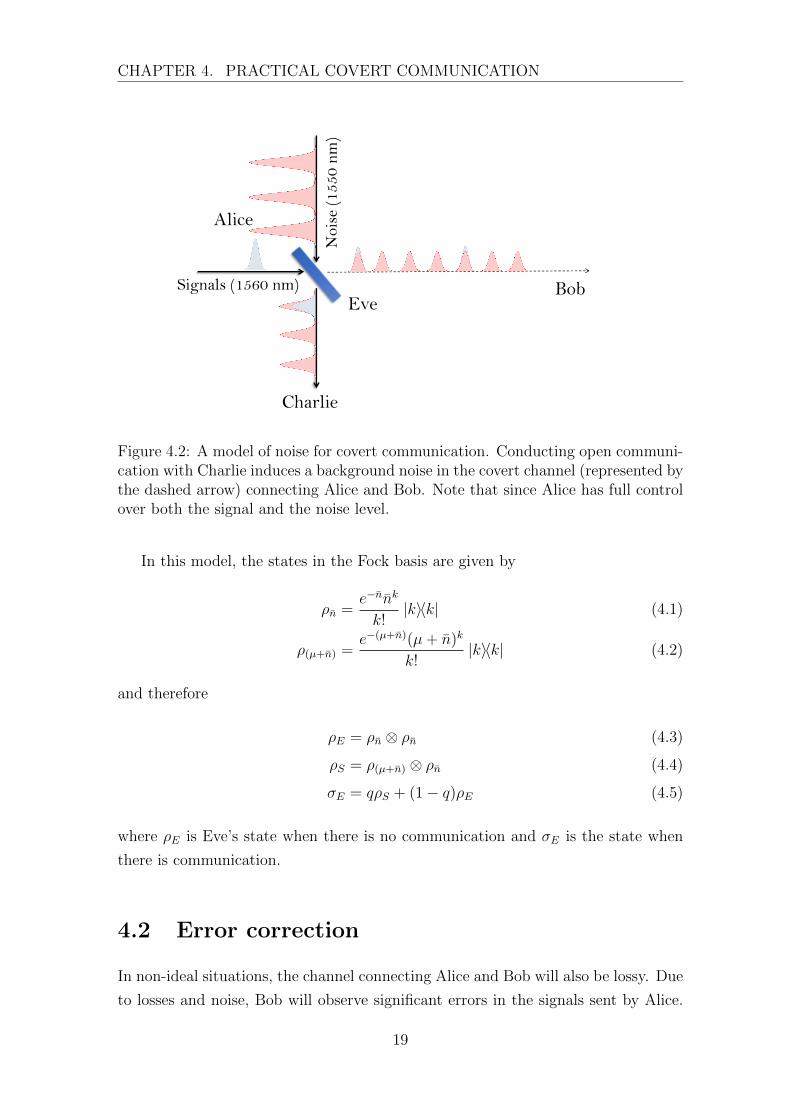
CHAPTER 4. PRACTICAL COVERT COMMUNICATION
Bob
Alice
EveSignals (1560 nm)
Nois
e (1
55
0 n
m)
Charlie
Figure 4.2: A model of noise for covert communication. Conducting open communi-cation with Charlie induces a background noise in the covert channel (represented bythe dashed arrow) connecting Alice and Bob. Note that since Alice has full controlover both the signal and the noise level.
In this model, the states in the Fock basis are given by
ρn =e−nnk
k!|k〉〈k| (4.1)
ρ(µ+n) =e−(µ+n)(µ+ n)k
k!|k〉〈k| (4.2)
and therefore
ρE = ρn ⊗ ρn (4.3)
ρS = ρ(µ+n) ⊗ ρn (4.4)
σE = qρS + (1− q)ρE (4.5)
where ρE is Eve’s state when there is no communication and σE is the state when
there is communication.
4.2 Error correction
In non-ideal situations, the channel connecting Alice and Bob will also be lossy. Due
to losses and noise, Bob will observe significant errors in the signals sent by Alice.
19
4.2. ERROR CORRECTION
To quantify Bob’s ability to decode Alice’s message correctly, we let Bob’s decoding
error probability be E . We want this probability to be reasonably low. Suppose
that Alice sends a message of length b bits, then Bob’s bit error probability δ can
be expressed in terms of E and b
δ = 1− (1− E)1/b (4.6)
Since for each of the N time-bins, Alice decides with equal probability q whether
or not she is going to send a signal, the expected number of signals d is given by
d = Nq (4.7)
In addition to the loss in the fiber, Bob’s detector will also have certain ineffi-
ciency. This will result in not all of the photons that Alice sends will be detected.
To model this loss, we consider a lossless channel, a perfect detector and a beam
splitter with transmitivity τ between them.
The probability pC that Bob detects a click in the correct mode is
pC = 1− Pr[no click in the correct mode]
= 1− exp[−τ(µ+ n)] (4.8)
while the probability pW that Bob detects a click in the wrong mode is
pW = 1− Pr[no click in the wrong mode]
= 1− exp(−τ n) (4.9)
Ignoring the probability of having clicks in both modes, the probability of having a
click is approximately (pC + pW ). Then, we get the probability that a click is in the
correct mode, given that there is a click is given by
pg =pC
pC + pW(4.10)
where pC and pW is given by (4.8) and (4.9) respectively.
Now, to correct these errors, we use the repetition code with majority vote
decoding scheme. Repetition code Rk repeats every bit k times such that
d = bk (4.11)
20
CHAPTER 4. PRACTICAL COVERT COMMUNICATION
For example, suppose Alice wants to send the bit ’0’. Instead of sending one ’0’ bit,
she will send the string′00...00...00′︸ ︷︷ ︸
k times
Next, Bob will look at the string he receives. Bob will decode the bit as ’0’ if he
receives more ’0’ bits than ’1’s, otherwise he will decode it as ’1’. We then obtain
an expression for δ
δ =k∑i=0
Pr[i clicks] Pr[correct clicks are not majority]
=k∑i=0
Pr[i clicks]
bi/2c∑j=0
Pr[j correct cliks |i clicks] (4.12)
The number of clicks C is binomially distributed with probability (pC +pW ) and
number of trials k. Now, since k is large and the probability of registering a click is
small, C is also approximately Poisson distributed. We let µC and σC be the mean
and standard deviation of the number of clikcs C respectively. It suffices to consider
the range of 5 standard deviations σC from the mean µC in the first summation in
equation (4.12). We get the equation
δ ≈µC+5σC∑i=µC−5σC
(k
i
)(pC + pW )i(1− pC − pW )k−i
bi/2c∑j=0
(i
j
)(pg)
j(1− pg)i−j (4.13)
≈µC+5σC∑i=µC−5σC
(µC)ie−µC
i!︸ ︷︷ ︸Poisson
bi/2c∑j=0
(i
j
)(pg)
j(1− pg)i−j︸ ︷︷ ︸Binomial
(4.14)
where for Poisson distribution, µC and σC are given by
µC = k × (pC + pW )
σC =√k × (pC + pW )
Using the above equations and (4.14), we can find the codeword length k that will
achieve the desired bit error probability δ.
4.3 Experimental implementation
In this section, we will describe some of the experimental considerations and con-
straints. To provide an overview of the experiment, we can refer to Fig. 4.3 for
21

4.3. EXPERIMENTAL IMPLEMENTATION
the experiment. We use the 1550 nm laser as the source for the noise and the 1560
nm laser for the signal. Note that while the experiment uses time-bin encoding, our
calculation assumes polarization encoding. However, we do not expect significant
differences.
Figure 4.3: Illustration of the experimental setup provided by our collaborators. Inthis experiment, Alice uses time-bin encoding. We use a sync laser and time-to-digital converter (TDC) to synchronize Alice’s and Bob’s clock. Both the signal andthe noise are passed through a beam splitter and go into the optical fiber. Bob usesthe superconducting single-photon detector (SSPD) to detect the photon. Then hedecodes the signal by measuring the time of arrival of the photon.
4.3.1 Loss and detector inefficiency
Due the losses in the fiber and detector inefficiency, some of the photons will not be
detected. To model this, we consider that there is no loss in the channel and the
detector is 100% efficient. However, we will add a beam splitter with transmittivity
τ across the channel. Based on the loss and the detector inefficiency, we approximate
the channel transmittivity to be τ ≈ 0.1.
4.3.2 Noise level
The noise level in the channel is fixed at 106 photons/s. However, we can adjust the
pulse width such that for each time-bin, we get the noise level that we desire. Thus,
22
CHAPTER 4. PRACTICAL COVERT COMMUNICATION
the mean photon number for the noise n is given by
n = 106w (4.15)
where w is the pulse width. We also note that the smallest pulse width that we can
achieve is wmin = 1 ns.
4.3.3 Extinction ratio
The extinction ratio re is given by
re =µon
µoff
(4.16)
where µon is the number of photons when the laser is on and µoff is the number of
photons when the laser is off.
For our experiment, the extinction ratio is 1000 : 1. This will affect our expression
for ρE. When we take into account the extinction ratio, it is given by
ρE =∑k
e−n′n′k
k!|k〉〈k| (4.17)
where n′ = n+ 0.001µ and |k〉 is the Fock state with photon number k.
4.4 Optimization of parameters
Now, we have all the necessary tools to perform our optimization. Since the upper
bound on the detection bias is a function of a number of parameters, namely the
mean photon number of the signal (µ) and the noise (n), as well as the probability
of sending a signal q. The probability of sending a signal, in turn, depends on the
number of of time-bins that are available (N), the length of the message b, and the
length of the repetition code (k), which depends on our tolerance on the decoding
error. Hence, in principle, optimizing the protocol is an optimization problem over
several number of parameters. Since it is challenging to do analytical optimization,
we will perform a numerical optimization over all the parameters (µ, n, q).
23

4.4. OPTIMIZATION OF PARAMETERS
4.4.1 Number of time-bins as objective function
To find the optimal performance of the protocol, we set a tolerance level for Eve’s
detection bias and Bob’s decoding error. Next, we fix the number of bits that Alice
is going to send and search for the values of µ and n that will achieve the desired
performance using the least number of time-bins. To do so, we have created a nu-
merical routine that outputs optimal values of µ and n for any protocol.
We aim to achieve the following performance:
• Number of bits in the message that Alice sends b = 35 bits (7 letters).
• Bob’s decoding error probability E = 0.01
• Eve’s detection bias ε = 0.1
Interestingly, when we have high signal-to-noise ratio, i.e. µ � n, Bob’s decod-
ing error is very small, hence Alice can send a smaller number of signals. However,
at the same time, high signal-to-noise ratio is also detrimental to the security of the
protocol because Eve can easily distinguish the bright signals from the noise. The
optimal region actually, lies in the low signal-to-noise ratio, where Eve has difficulty
distinguishing signals and noise, but Bob can still, through a large enough code
length, retrieve the messages reliably.
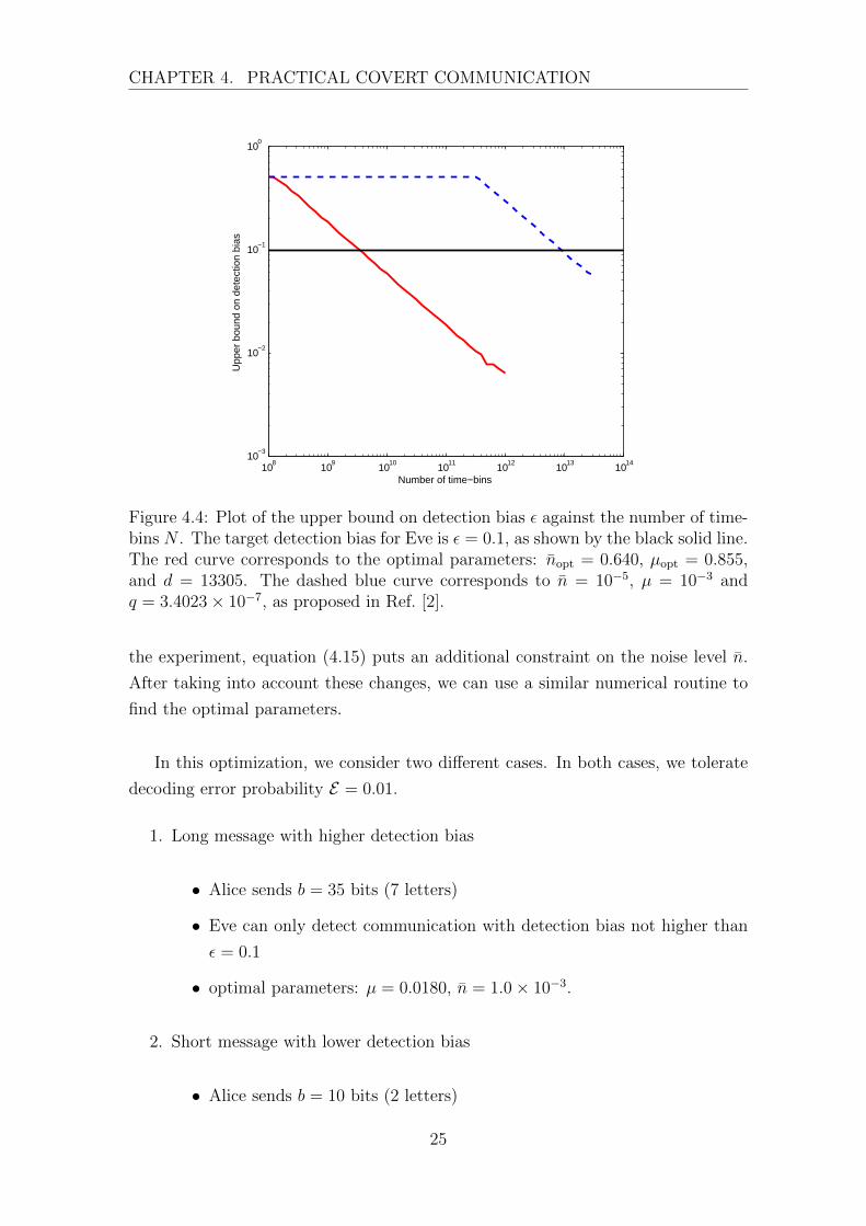
A plot of the protocol performance with optimal parameters is shown in Fig. 4.4.
As it can be clearly seen, compared to the values suggested in Ref. [2], which rely
on thermal background noise at infrared frequencies, our protocol offers a reduction
in the number of time-bins of several orders of magnitude.
4.4.2 Time as objective function
In most practical situations, the important resource is time. As such, it may be
more important to minimize the duration of the protocol rather than minimizing
the number of time-bins (number of channel uses). For a given pulse width w, the
total time needed to execute the protocol t is related to the total number of time-bins
N by
t = Nw (4.18)
We also have to keep in mind that w is determined uniquely by equation (4.15).
Therefore, in finding the optimal parameters that will minimize the running time of
24
CHAPTER 4. PRACTICAL COVERT COMMUNICATION
108
109
1010
1011
1012
1013
1014
10−3
10−2
10−1
100
Number of time−bins
Upp
er b
ound
on
dete
ctio
n bi
as
Figure 4.4: Plot of the upper bound on detection bias ε against the number of time-bins N . The target detection bias for Eve is ε = 0.1, as shown by the black solid line.The red curve corresponds to the optimal parameters: nopt = 0.640, µopt = 0.855,and d = 13305. The dashed blue curve corresponds to n = 10−5, µ = 10−3 andq = 3.4023× 10⁻⁷, as proposed in Ref. [2].
the experiment, equation (4.15) puts an additional constraint on the noise level n.
After taking into account these changes, we can use a similar numerical routine to
find the optimal parameters.
In this optimization, we consider two different cases. In both cases, we tolerate
decoding error probability E = 0.01.
1. Long message with higher detection bias
• Alice sends b = 35 bits (7 letters)
• Eve can only detect communication with detection bias not higher than
ε = 0.1
• optimal parameters: µ = 0.0180, n = 1.0× 10⁻³.
2. Short message with lower detection bias
• Alice sends b = 10 bits (2 letters)
25
4.4. OPTIMIZATION OF PARAMETERS
• Eve can only detect communication with detection bias not higher than
ε = 0.01
In both cases, we obtain the optimal noise level n = 0.001 as this corresponds
to the smallest pulse width that we can achieve w = 1 ns. In this optimization, the
optimal signal-to-noise ratio is not very low. Due to the physical constraints that
force us to operate at much lower n and µ (unlike in our first optimization where
both nopt and µopt are relatively high), means that we need higher mean photon
numbers for the signal to accommodate the losses in the channel.
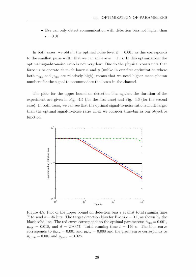
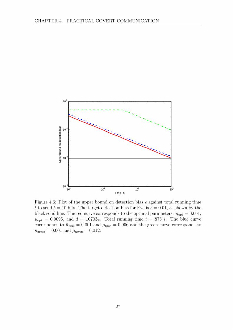
The plots for the upper bound on detection bias against the duration of the
experiment are given in Fig. 4.5 (for the first case) and Fig. 4.6 (for the second
case). In both cases, we can see that the optimal signal-to-noise ratio is much larger
than the optimal signal-to-noise ratio when we consider time-bin as our objective
function.
100
101
102
103
10−2
10−1
100
Time / s
Upp
er b
ound
on
dete
ctio
n bi
as
Figure 4.5: Plot of the upper bound on detection bias ε against total running timeT to send b = 35 bits. The target detection bias for Eve is ε = 0.1, as shown by theblack solid line. The red curve corresponds to the optimal parameters: nopt = 0.001,µopt = 0.018, and d = 208357. Total running time t = 146 s. The blue curvecorresponds to nblue = 0.001 and µblue = 0.008 and the green curve corresponds tongreen = 0.001 and µgreen = 0.028.
26
CHAPTER 4. PRACTICAL COVERT COMMUNICATION
100
101
102
103
10−3
10−2
10−1
100
Time / s
Upp
er b
ound
on
dete
ctio
n bi
as
Figure 4.6: Plot of the upper bound on detection bias ε against total running timet to send b = 10 bits. The target detection bias for Eve is ε = 0.01, as shown by theblack solid line. The red curve corresponds to the optimal parameters: nopt = 0.001,µopt = 0.0095, and d = 107034. Total running time t = 875 s. The blue curvecorresponds to nblue = 0.001 and µblue = 0.006 and the green curve corresponds tongreen = 0.001 and µgreen = 0.012.
27

4.4. OPTIMIZATION OF PARAMETERS
28
Chapter 5
Other Attempts to Improve
Covert Communication Protocols
In the previous chapter, we optimized the protocol by only considering the experi-
mental parameters. In this chapter, we consider other strategies that Alice can use.
In other words, we want to consider some modifications to our basic protocol. Here,
we consider the case where the number of channel uses is the objective function.
5.1 Block implementation of covert communica-
tion
Now, consider the protocol where access to N channel uses corresponds to an access
to N time-bins. Suppose Alice and Bob have K blocks, each containing N time-
bins. For each block, Alice independently decides with probability p whether she
will perform the basic protocol and with probability (1− p), she will do nothing in
that block of N time-bins. For each block, let
ρ = (ρE)⊗N
σ = (σE)⊗N
where ρE and σE is the same as before. Now let σ∗ be
σ∗ = pσ + (1− p)ρ (5.1)
29
5.2. SENDING MULTIPLE BITS PER PHOTON
Thus, Eve’s 2KN -mode state is given by
ρ′ = ρ⊗K (5.2)
σ′ = (σ∗)⊗K = (pσ + (1− p)ρ)⊗K (5.3)
The detection bias ε for the block protocol is bounded by
ε ≤√
1
8D(ρ′||σ′) =
√K
8D(ρ||σ∗)
=
√K
8D(ρ||(pσ + (1− p)ρ))
≤√K
8pD(ρ||σ) =
√NK
8pD(ρE||σE) (5.4)
where we used the joint convexity of relative entropy, that is for states ρ1, ρ2, σ1, σ2
and for all 0 ≤ p ≤ 1, we have from Theorem 2.3.3
D(pρ1 + (1− p)ρ2||pσ1 + (1− p)σ2) ≤ pD(ρ1||σ1) + (1− p)D(ρ2||σ2) (5.5)
and by setting
ρ1 = ρ2 = σ2 = ρ
σ1 = σ
the second term in (5.5) vanishes and we get the inequality that we want.
If we want the expected number of signals d to be the same, we need p = 1/K
and thus we get back the bound that we had in the original protocol and there is
no improvement.
5.2 Sending multiple bits per photon
Alice can also consider encoding multiple bits into a single photon. She can do this
by exploring other degrees of freedom of the photon (for example we can consider
both polarization and time of arrival of the photon). By encoding more bits into
a photon, she hopes that it would be harder for Eve to detect the communication
since Alice can send less number of photons to send the same number of bits.
30

CHAPTER 5. OTHER ATTEMPTS TO IMPROVE COVERTCOMMUNICATION PROTOCOLS
5.2.1 Eve’s states and detection bias
For fair comparison, we assume that Alice and Bob still have access to 2N modes.
Suppose Alice encodes M bits into one photon. Now, for each channel use, the state
when there is no communication
ρ′E = ρ⊗2M
n (5.6)
and the signal state is given by
ρ′S = ρ(µ+n) ⊗ ρ⊗(2M−1)n (5.7)
where ρ(µ+n) is the same as in (4.2). Eve’s state when there is communication is
therefore given by
σ′E = q′ρ′S + (1− q′)ρ′E (5.8)
where q′ is given by
q′ =bk/M
2N/2M=
2M−1
Mq (5.9)
Eve’s 2N -mode states are given by
ρ = (ρ′E)⊗N/2M−1
(5.10)
σ = (σ′E)⊗N/2M−1
(5.11)
Therefore the upper bound on detection bias is given by
ε ≤ 1√2M−1
√N
8D(ρ′E||σ′E) (5.12)
We can check that we obtain the formulae in Chapter 4 when M = 1. The factor
of 1/√
2M−1 is favourable for covert communication. However, we can easily check
that q′ > q for M > 2. This will increase the relative entropy and therefore the
detection bias. Additionally, we have not taken into account any effect on Bob’s
reliability in decoding the message.
5.2.2 Decoding error probability
Since we operate at multiple modes, Bob’s error probability will be different from
our basic scheme’s. The probability pC that the detector detects a photon in the
31
5.2. SENDING MULTIPLE BITS PER PHOTON
correct mode is still the same
pC = 1− Pr[no click in the correct mode]
= 1− exp[−τ(µ+ n)] (5.13)
while the probability pW that the detector detects a photon in one of the wrong
modes is given by
pW = 1− Pr[no click in any of the wrong modes]
= 1− exp(−τ n)(2M−1) (5.14)
For any M > 1, pW in (5.14) is larger than pW in (4.9). It follows that the proba-
bility pg that a click is in the right mode, given that there is a click, is smaller.
Meanwhile, the relationship between decoding error probability E and δ will be
δ = 1− (1− E)M/b (5.15)
Note that δ no longer of the interpretation as bit error probability since each signal
now contains M bits of information.
For error correction, if we use repetition code of length k, to guarantee correct
decoding, we demand that there should be at least (bk/2c+ 1) clicks in the correct
mode. Typically, a smaller number is sufficient to achieve majority, however, in the
worst case scenario (where all the errors are contributed by the same mode), we
need at least that number of clicks. Therefore, the expression for δ in (4.14) is still
valid in this protocol.
Since pW is larger in this protocol, we need longer codeword to correct the errors.
Consequently, we will need more time-bins if we want to keep the probability of
sending a signal q unchanged.
5.2.3 Numerical results
Since it is inconclusive from our analysis whether there will be an improvement to
the protocol, we will do numerical optimization of the new scheme. We will con-
sider the case where M = 2 and M = 3 (as q′ increases with M , we do not expect
improvement in higher values of M) and compare it to the basic protocol (M = 1).
32

CHAPTER 5. OTHER ATTEMPTS TO IMPROVE COVERTCOMMUNICATION PROTOCOLS
Unfortunately, it turns out that the modification does not improve the efficiency
of the protocol even after the optimization of the parameters. We observes that
increasing the number of bits encoded in one photon actually worsens the perfor-
mance of the protocol as shown in Fig. 5.1. We learn that it is not enough to
increase the length of the repetition code to compromise the increase in pW . Alice
needs to increase her signal-to-noise ratio, which leads to higher detection bias.
107
108
109
1010
1011
1012
10−3
10−2
10−1
100
Number of time−bins
Upp
er b
ound
on
dete
ctio
n bi
as
M = 1M = 2M = 3
ε = 0.1
Figure 5.1: The plot of the upper bound on detection bias ε against the number oftime-bins N to send a message of length b = 35 bits. We set the decoding errorprobability E = 0.01. The red curve corresponds to our basic protocol where we sendone bit per photon. The mean photon numbers are µred = 0.855 and nred = 0.640for the signal and the noise respectively. The blue dotted curve corresponds to thecase when we encode two bits into per photon with µblue = 0.170 and nblue = 0.021.The green dashed curve corresponds to the case when we encode three bits into perphoton with µgreen = 0.160 and ngreen = 0.007. The horizontal black line is thetarget detection bias ε = 0.1.
5.3 Switching-off the noise
In situations when Alice has full control over both the signal and the noise level,
like the one discussed in Chapter 4, one could think of turning-off the noise when a
signal is sent. In implementation like ours (Fig. 4.1), this may be problematic since
the modes are different: by sitting at 1550 nm, Eve could notice that there is no
33

5.3. SWITCHING-OFF THE NOISE
light when a covert signal is sent. By assuming implementations where the modes
are equal, like the one in Chapter 3, does this actually help? Here, we prove that it
doesn’t.
In this implementation of the protocol, when a signal is sent, Bob will no longer
get a click from the noise. However, as the noise does not contribute to the error,
now we need to take into account the error coming from the alignment of Bob’s
polarizing beam splitter (PBS). Suppose Alice sends a photon with horizontal po-
larization, when Bob’s PBS is not perfectly aligned, the PBS sees some vertical
component in the photon’s polarization. There is a non-zero probability that the
photon’s polarization is measured as vertical. In this section, we will consider im-
perfect alignment as the main source of error, which is insignificant in our original
scheme.
On the other hand, now Eve can also distinguish the noise level when there is a
communication and when there is no communication. Intuitively, this will increase
her detection bias. Thus, we need to perform optimization of this protocol and see
whether the overall effect will lead to an improvement.
This modification can be applied to both the original protocol and the proto-
col where Alice encodes multiple bits into one photon. As the main drawback of
the multiple bits per photon scheme is the increase in error, this modification can
eliminate the problem.
5.3.1 Single bit per photon
When Alice encodes one bit per photon, the expression for signal state is replaced
by
ρS = ρµ ⊗ |0〉〈0| (5.16)
where ρµ is the coherent state with mean photon number µ and phase-randomization
and |0〉 is the vacuum state.
The state when there is communication in the channel is given by
σE = q(ρµ ⊗ |0〉〈0|) + (1− q)(ρn ⊗ ρn) (5.17)
34

CHAPTER 5. OTHER ATTEMPTS TO IMPROVE COVERTCOMMUNICATION PROTOCOLS
To calculate Bob’s bit error probability, we model the imperfect alignment as a
beam splitter that sometimes reflects a photon to the wrong mode. Let v be the
transmittivity of Bob’s beam splitter. Then the probability pC that Bob detects a
photon in the correct mode
pC = 1− exp(−τµv) (5.18)
while the probability pW that Bob get a click in the wrong mode is
pW = 1− exp(−τµ(1− v)) (5.19)
5.3.2 Multiple bits per photon
When Alice encodes M bits into one photon, the expression for the signal state is
ρS = ρµ ⊗ |0〉〈0|⊗(2M−1) (5.20)
The probability of sending a photon is given by (5.9).
To compute δ (here, we use the expression of δ in (5.15)), we use the same model
for the alignment of Bob’s PBS. The expression for the probability of having click in
the correct mode (pC) is the same as (5.18) while to calculate pW we also consider
the following sources of error:
1. Imperfect alignment of the PBS.
2. Dark count of Bob’s detector. We let the detector to have a dark count at
constant rate of PD = 10−6.
Therefore, the probability of Bob having a click in the wrong mode is given by
pW = 1− exp(−τµ(1− v))︸ ︷︷ ︸alignment
(1− PD)2M−2︸ ︷︷ ︸dark count
(5.21)
5.3.3 Evaluation of the protocol
Taking into account the extinction ratio, we change the vacuum state |0〉〈0| to the
coherent state ρn′ with mean photon number n′ = n/re = 0.001n. However, after
optimization, the overall performance of both protocols (single bits per photon and
multiple bits per photon) is still significantly below the basic protocol. We conclude
35
5.4. MULTIPLEXING
that the effect of switching-off the noise on the detection bias is more significant
than its effect on the decoding error. Thus, this modification fails to improve the
efficiency of covert communication.
5.4 Multiplexing
Multiplexing is a method by which the multiple signals are combined into one sig-
nal over shared medium. A common technique of multiplexing is the frequency-
division multiplexing (or sometimes called the wavelength-division multiplexing).
Frequency-division multiplexing (FDM) allows a number of signals to be modulated
onto different carrier frequencies and then carried simultaneously. It is used widely
in our day-to-day communication technologies, such as radio and television set. To
perform frequency-division multiplexing, the bandwidth of the medium must exceed
the bandwidth of the signals. Secondly, the carrier frequencies must be well sepa-
rated such that the bandwidth of the signals do not overlap [9]. In this section, we
are looking of the possibility of implementing frequency-division multiplexing of the
noise in covert communication to shorten the duration of the experiment.
The noise level in the channel connecting Alice and Bob depends on the profile of
the intensity of the source as a function of wavelength by which they communicate.
For concreteness, we assume that Alice and Bob communicates in two different
carrier wavelengths λ1 and λ2 and the noise level in these two wavelength is given
by
n1 ≡ n(λ1) (5.22)
n2 ≡ n(λ2) (5.23)
Similarly, for the mean photon number of the signal
µ1 ≡ µ(λ1) (5.24)
µ2 ≡ µ(λ2) (5.25)
We define the effective number of channel uses T
T ≡ t
w(5.26)
where t is the duration of the experiment and w is the pulse width.
36
CHAPTER 5. OTHER ATTEMPTS TO IMPROVE COVERTCOMMUNICATION PROTOCOLS
Now if T0 is the effective number of channel uses when we do not use FDM, then
T0 = N (5.27)
where N is the total number of channel uses. Therefore, when we use FDM, we get
T =N
2(5.28)
since for every pulse, we use the channel twice (we use both the λ1 and λ2 channel).
In general, Alice does not need to send equal number of signals in the two
frequencies. In other words, suppose Alice is sending b bits to Bob, she can send ηb
bits in λ1 and (1−η)b bits in λ2 where 0 ≤ η ≤ 1. Furthermore, for error correction,
the length of the codewords sent in λ1 would be different from the length of the
codewords sent in λ2. Thus, the number of signals sent in each wavelength is given
by
d1 = ηbk1 (5.29)
d2 = (1− η)bk2 (5.30)
where d1 and d2 are the number of signals sent in λ1 and λ2 with k1 and k2 as
the length of the codewords in the respective wavelength. Then, the probability of
sending a signal in each wavelength is given by
q1 =d1
N/2(5.31)
q2 =d2
N/2(5.32)
Now, let
ρ1 = ρn1 ⊗ ρn1 (5.33)
ρS1 = ρ(µ1+n1) ⊗ ρn1 (5.34)
ρ2 = ρn2 ⊗ ρn2 (5.35)
ρS2 = ρ(µ2+n2) ⊗ ρn2 (5.36)
where ρniand ρ(µi+ni) are coherent states with mean photon number ni and (µi+ ni)
37

5.4. MULTIPLEXING
respectively and i = 1, 2. We also let
σ1 = q1ρS1 + (1− q1)ρ1 (5.37)
σ2 = q2ρS2 + (1− q2)ρ2 (5.38)
Then, we can compute Eve’s states
ρ = ρ⊗N/21 ⊗ ρ⊗N/22 (5.39)
σ = σ⊗N/21 ⊗ σ⊗N/22 (5.40)
Thus, the detection bias is bounded by
ε ≤
√1
8
N
2
(D(ρ1||σ1) +D(ρ2||σ2)
)(5.41)
By the same token, we can further generalize the protocol to allow communica-
tion in X wavelengths by setting
di = ηibki (5.42)
qi =di
N/X(5.43)
ε ≤
√√√√1
8
N
X
X∑i=1
D(ρi||σi) (5.44)
T =N
X(5.45)
where i = 1, 2, ..., X and∑
i ηi = 1. However, considering the number of parame-
ters that are involved, we will not optimize the protocol for the most general case.
Instead, we will optimize the protocol in which Alice and Bob communicate in two
wavelengths simultaneously. In this case, the parameters that we need to consider
are η, n1, n2, µ1, µ2.
For optimal performance of the protocol, we demand that
n1 = nopt (5.46)
µ1 = µopt (5.47)
where nopt and µopt are the optimal mean photon number of the noise and the signal
in the basic protocol.
38

CHAPTER 5. OTHER ATTEMPTS TO IMPROVE COVERTCOMMUNICATION PROTOCOLS
Furthermore, since λ1 is the more efficient wavelength for the communication,
we want to send more bits in λ1 than in λ2. We can set
η ≥ 1− η
⇒ η ≥ 1
2(5.48)
In general, whether multiplexing leads to an improvement in the protocol de-
pends on how the noise level depends on the wavelengths in which the communi-
cation take place. In this report, we do not consider a particular function which
governs the relationship of the noise level with the wavelength associated to the
channel. Instead, we consider how different noise level and evaluate what is the
range of noise level, in which multiplexing is suitable.
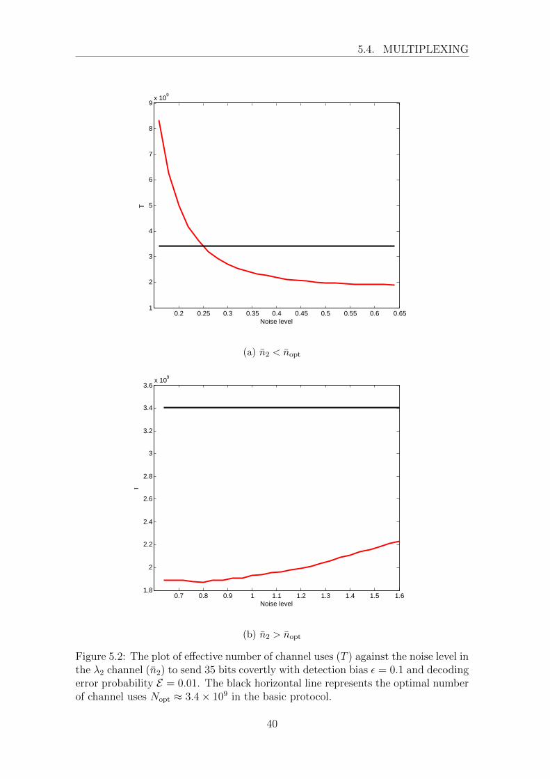
Again, we consider the case where Alice sends b = 35 bits covertly, with Eve’s
detection bias of ε = 0.1 and Bob’s decoding error probability E = 0.01. As some
may have expected, the optimal case is when n2 = nopt and µ2 = µopt as well with
η = 0.5. In this case, we have
T = 1.8951× 10⁹ ≈ Nopt
2(5.49)
where Nopt is the optimal number of channel uses in the original protocol.
We may also be interested to know whether we still get an improvement when
the n2 differs from the optimal noise level. Suppose we can achieve µ2 = µopt and
setting η = 0.5, we want to know how much deviation from optimal noise level can
we tolerate while still having an improvement from multiplexing. In Fig. 5.2, we
plot the graph of the effective number of channel uses (T ) against the noise level in
λ2 channel (n2).
We can see that multiplexing can lead to improvement in relatively large range
of noise level (from less than half of the optimal noise level to more than twice
of the optimal noise level). Although this result may sound promising, whether
multiplexing is practically feasible also depends on the relationship of the noise level
and the wavelength in which the communication take place.
39
5.4. MULTIPLEXING
0.2 0.25 0.3 0.35 0.4 0.45 0.5 0.55 0.6 0.651
2
3
4
5
6
7
8
9x 10
9
Noise level
T
(a) n2 < nopt
0.7 0.8 0.9 1 1.1 1.2 1.3 1.4 1.5 1.61.8
2
2.2
2.4
2.6
2.8
3
3.2
3.4
3.6x 10
9
Noise level
T
(b) n2 > nopt
Figure 5.2: The plot of effective number of channel uses (T ) against the noise level inthe λ2 channel (n2) to send 35 bits covertly with detection bias ε = 0.1 and decodingerror probability E = 0.01. The black horizontal line represents the optimal numberof channel uses Nopt ≈ 3.4× 10⁹ in the basic protocol.
40

Chapter 6
Conclusion
6.1 Summary
The recent developments in covert communication has made it very important to
optimize the performance of covert communication protocols in order to bring them
closer to practical demonstrations. To do that, we propose a model where the noise
in Alice-Bob channel arises from the leakage in Alice-Charlie channel where an open
communication is taking place. Using this model, we minimize the number of chan-
nel uses and the time taken to send a classical message covertly.
Our method of optimization is as follows. First, we set a target for detection bias
and tolerance on Bob’s decoding error probability. Next, we perform a numerical
routine to find the experimental parameters that will minimize the number of time-
bins or the time taken to perform the experiment. We discovered that the optimal
signal-to-noise ratio that will minimize the number of channel uses is relatively low.
This causes difficulty for Eve to distinguish the signal-to-noise ratio, but Bob can
still decode the message reliably through sufficiently large code length. On the other
hand, the optimal mean photon number of both the signal and the noise is relatively
small when we want to minimize the duration of the protocol. This is because the
lower noise level corresponds to smaller pulse width, which is an important factor
which affects the duration of the experiment. To compromise the loss in the fiber,
we need a sufficiently high mean photon number for the signal. Thus, we have a
slightly higher signal-to-noise ratio compared to the case where we want to minimize
the number of channel uses.
Finally, we considered variations on the encoding or implementations of the pro-
tocol but, other than multiplexing, none of those provide any advantage over the
41
6.2. FUTURE DIRECTIONS
basic scheme.
6.2 Future directions
In this project, we consider the implementation of covert communication in blocks
where Alice decides in i.i.d. manner whether she will perform the protocol in that
block. This scheme is easy to analyze, however Alice can, in principle, use a different
strategy in which she randomly choose only one block where she will perform the
covert communication protocol. Although it would be more difficult to analyze the
performance of such protocol, since the state will not be of tensor products struc-
ture, it is interesting to know whether this modification will lead to an improvement.
In our model, we consider noise that is induced by communication using bright
signals in the neighbouring channel. Although this gives Alice the ability of con-
trolling the noise level in the channel, such source of noise is rather artificial. The
fact that Alice and Bob is connected by an optical fiber may also be incriminating
to them. We can consider a covert communication protocol that is performed in
free space subjected to the noise naturally present in daylight. The difficulty in this
protocol is in modeling the state for daylight as well as the usual challenges in free
space communication.
So far, we only considered the covert transmission of classical information. It
would also be interesting to perform an optimization of quantum covert communi-
cation protocol. For example, one could look at the signals as encoding a qubit and
perform state tomography to reconstruct its state.
42
Appendix A
Calculation of the Signal State
In this appendix, we present the explicit calculation of the signal state ρS. The
signal state ρS can be computed directly by considering Eve’s state when there is k
photons coming from the noise and l photons coming from the signal. We denote
that state by σkl. As discussed in section 3.3.2, it is sufficient to consider only few
number of photons, so we will only consider k ≤ 1 and l ≤ 2.
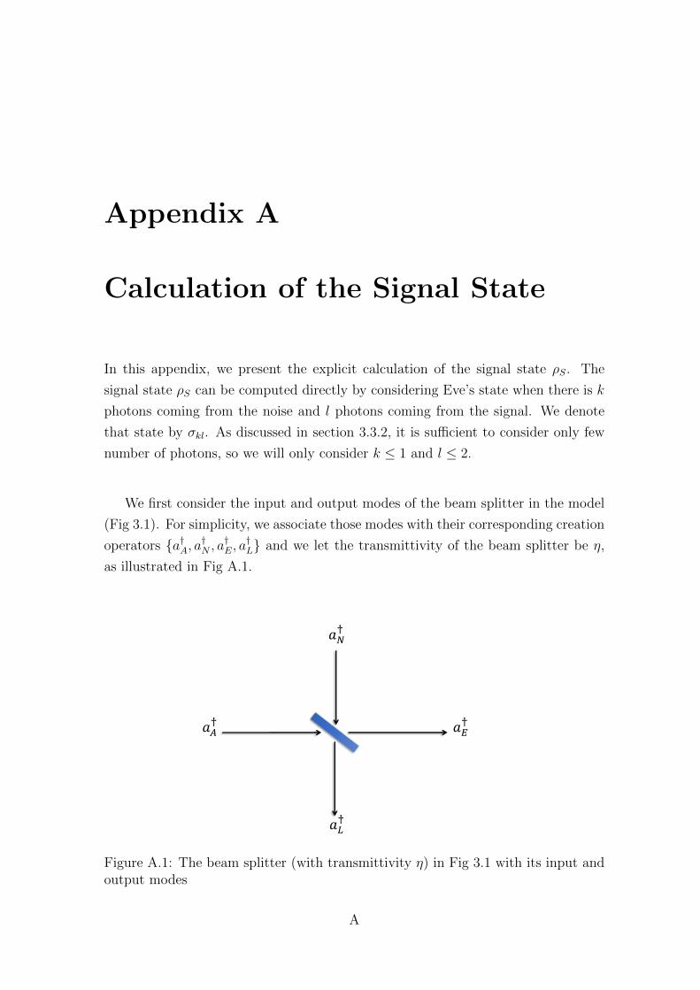
We first consider the input and output modes of the beam splitter in the model
(Fig 3.1). For simplicity, we associate those modes with their corresponding creation
operators {a†A, a†N , a
†E, a
†L} and we let the transmittivity of the beam splitter be η,
as illustrated in Fig A.1.
𝑎𝐴† 𝑎𝐸
†
𝑎𝑁†
𝑎𝐿†
Figure A.1: The beam splitter (with transmittivity η) in Fig 3.1 with its input andoutput modes
A

The transformation of the beam splitter can be written as
a†A →√ηa†E + i
√1− ηa†L
a†N →√ηa†L + i
√1− ηa†E
Using this transformation rule, we will compute the σkl’s. In this appendix, we will
adopt the convention of |nEnL〉 for the Fock state describing nE photons in the E
mode and nL photons in the L mode.
Computing σ00 is trivial. Since we have vacuum in both input modes A and N ,
we will also have vacuum in both output modes E and L. Thus
σ00 = |0〉〈0|
For σ01, we have
a†A |vac〉〈vac| aA → (√ηa†E + i
√1− ηa†L) |vac〉〈vac| (√ηaE − i
√1− ηaL)
= η |10〉〈10|+ (1− η) |01〉〈01|+ i√η(1− η) |10〉〈01|
− i√η(1− η) |01〉〈10|
≡ σ′01
To obtain σ01, we take the partial trace of σ′01 with respect to L.
σ01 = TrL(σ′01)
= (1E ⊗ 〈0|L)σ′01(1E ⊗ |0〉L) + (1E ⊗ 〈1|L)σ′01(1E ⊗ |1〉L)
= (1− η) |0〉〈0|+ η |1〉〈1|
Therefore, we can see that the effect of taking partial trace is removing the off-
diagonal terms of the E-L system, and then only keeping nE in the remaining
|nEnL〉〈nEnL|’s. As such, we will skip the details of the partial trace step for rest of
the σkl’s.
For σ02:
σ02 = TrL
[1√2
(√ηa†E + i
√1− ηa†L)2 |vac〉〈vac| (√ηaE − i
√1− ηaL)
1√2
]=
1
2TrL
[(η(a†E)2 + 2i
√η(1− η)a†Ea
†L − (1− η)2(a†L)2
)|vac〉
〈vac|(ηa2
E − 2i√η(1− η)aEaL − (1− η)2a2
L
)]B

APPENDIX A. CALCULATION OF THE SIGNAL STATE
σ02 = (1− η)2 |0〉〈0|+ 2η(1− η) |1〉〈1|+ η2 |2〉〈2|
For σ10:
σ10 = TrL
[(√ηa†L + i
√1− ηa†E) |vac〉〈vac| (√ηaL − i
√1− ηaE)
]= η |0〉〈0|+ (1− η) |1〉〈1|
For σ11:
σ11 = TrL
[(√ηa†E + i
√1− ηa†L)(
√ηa†L + i
√1− ηa†E) |vac〉
〈vac| (√ηaE − i√
1− ηaL)(√ηaL − i
√1− ηaE)
]= TrL
[((2η − 1)a†Ea
†L + i
√η(1− η)(a†L)2 + i
√η(1− η)(a†E)2
)|vac〉
〈vac|(
(2η − 1)aEaL − i√η(1− η)a2
L − i√η(1− η)a2
E
)]= 2η(1− η) |0〉〈0|+ (1− 2η)2 |1〉〈1|+ 2η(1− η) |2〉〈2|
For σ12:
σ12 = TrL
[1√2
(√ηa†E + i
√1− ηa†L)2(
√ηa†L + i
√1− ηa†E) |vac〉
〈vac| (√ηaL − i√
1− ηaE)(√ηaE − i
√1− ηaL)2 1√
2
]=
1
2TrL
[(iη√
(1− η)(a†E)3 + (3η − 2)√η(a†E)2a†L + i(3η − 1)
√1− ηa†E(a†L)2
− (1− η)√η(a†L)3
)|vac〉〈vac|
(− iη
√(1− η)a3
E + (3η − 2)√ηa2
EaL
− i(3η − 1)√
1− ηaEa2L − (1− η)
√ηa3
L
)]= 3η(1− η)2 |0〉〈0|+ (1− η)(1− 3η)2 |1〉〈1|+ η(2− 3η)2 |2〉〈2|+ 3η2(1− η) |3〉〈3|
In summary, these are the six σkl’s that we compute
σ00 = |0〉〈0| (A.1)
σ01 = (1− η) |0〉〈0|+ η |1〉〈1| (A.2)
σ02 = (1− η)2 |0〉〈0|+ 2η(1− η) |1〉〈1|+ η2 |2〉〈2| (A.3)
σ10 = η |0〉〈0|+ (1− η) |1〉〈1| (A.4)
σ11 = 2η(1− η) |0〉〈0|+ (1− 2η)2 |1〉〈1|+ 2η(1− η) |2〉〈2| (A.5)
C

σ12 = 3η(1− η)2 |0〉〈0|+ (1− η)(1− 3η)2 |1〉〈1|
+ η(2− 3η)2 |2〉〈2|+ 3η2(1− η) |3〉〈3| (A.6)
Using those six states, we can calculate the signal state ρS using
ρS ≈1∑
k=0
2∑l=0
nk
(1 + n)k+1
e−µµl
l!σkl
D
Bibliography
[1] Arrazola, J. M., and Lutkenhaus, N. Quantum communication with
coherent states and linear optics. Phys. Rev. A 90 (Oct 2014), 042335.
[2] Arrazola, J. M., and Scarani, V. Covert quantum communication. Phys.
Rev. Lett. 117 (Dec 2016), 250503.
[3] Bash, B. A., Gheorghe, A. H., Patel, M., Habif, J. L., Goeckel,
D., Towsley, D., and Guha, S. Quantum-secure covert communication on
bosonic channels. Nature communications 6 (2015).
[4] Bash, B. A., Goeckel, D., and Towsley, D. Limits of reliable commu-
nication with low probability of detection on awgn channels. IEEE Journal on
Selected Areas in Communications 31, 9 (2013), 1921–1930.
[5] Helstrom, C. W. Quantum Detection and Estimation Theory. Academic
Press New York, 1976.
[6] Sanguinetti, B., Traverso, G., Lavoie, J., Martin, A., and Zbinden,
H. Perfectly secure steganography: Hiding information in the quantum noise
of a photograph. Phys. Rev. A 93 (Jan 2016), 012336.
[7] Scarani, V., Bechmann-Pasquinucci, H., Cerf, N. J., Dusek, M.,
Lutkenhaus, N., and Peev, M. The security of practical quantum key
distribution. Rev. Mod. Phys. 81 (Sep 2009), 1301–1350.
[8] Shankar, R. Principles of Quantum Mechanics. Springer Science & Business
Media, 2012.
[9] Stallings, W. Data and Computer Communications, 4 ed. Maxwell Macmil-
lan International, 1994.
[10] Wilde, M. M. Quantum Information Theory. Cambridge University Press,
2013.
E
Related Documents