Optimization of Parameters of Asymptotically Stable Systems

Hindawi Publishing CorporationMathematical Problems in EngineeringVolume 2011, Article ID 526167, 19 pagesdoi:10.1155/2011/526167

Research ArticleOptimization of Parameters of AsymptoticallyStable Systems

Anna Guerman,1 Ana Seabra,2 and Georgi Smirnov3

1 Department of Electromechanical Engineering, Centre for Aerospace Science and Technologies, UBI,University of Beira Interior, Calcada Fonte do Lameiro, 6201-001 Covilha, Portugal

2 Scientific Area of Mathematics, ESTGV, Polytechnic Institute of Viseu, Campus Politecnico,3504-510 Viseu, Portugal

3 Department of Mathematics and Applications, School of Sciences, Centre of Physics, University of Minho,Campus de Gualtar, 4710-057 Braga, Portugal

Correspondence should be addressed to Ana Seabra, [email protected]

Received 29 June 2010; Revised 14 November 2010; Accepted 26 January 2011

Academic Editor: Oded Gottlieb

Copyright q 2011 Anna Guerman et al. This is an open access article distributed under theCreative Commons Attribution License, which permits unrestricted use, distribution, andreproduction in any medium, provided the original work is properly cited.

This work deals with numerical methods of parameter optimization for asymptotically stablesystems. We formulate a special mathematical programming problem that allows us to determineoptimal parameters of a stabilizer. This problem involves solutions to a differential equation. Weshow how to chose the mesh in order to obtain discrete problem guaranteeing the necessaryaccuracy. The developed methodology is illustrated by an example concerning optimization ofparameters for a satellite stabilization system.

1. Introduction

Consider differential equation

x = f(x, u), x ∈ Rn, t ≥ 0, (1.1)

that describes a system equipped with a stabilizer. Here, u ∈ U ⊂ Rk is a parameter. It isassumed that 0 = f(0, u) for all u ∈ U and the zero equilibrium position of system (1.1)is asymptotically stable whenever u ∈ U. The parameter u should be chosen to optimize,in some sense, the behaviour of the trajectories. The choice of this parameter can be basedon various criteria; obviously, it is impossible to construct a stabilizer optimal in all aspects.For example, for a linear controllable system, the pole assignment theorem guarantees the

2 Mathematical Problems in Engineering

existence of a linear feedback yielding a linear differential equation with any given set ofeigenvalues. One can choose a stabilizer with a very high damping speed. However, such astabilizer is practically useless because of the so called pick-effect (see [1, 2]). Namely, thereexists a large deviation of the solutions from the equilibrium position at the beginning of thestabilization process, whenever the module of the eigenvalues is big.

The aim of this paper is to develop an effective numerical tool oriented to optimizationof stabilizer parameters according to different criteria that appear in the engineeringpractice.

Throughout this paper, we denote the set of real numbers by R and the usual n-dimensional space of vectors with components inR byRn. The space of absolutely continuousfunctions defined in [0, T]with values inRn is denoted by AC([0, T], Rn). We denote by 〈a, b〉the usual scalar product in Rn and by | · | the Euclidean norm. By B, we denote the closed unitball, that is, the set of vectors x ∈ Rn satisfying |x| ≤ 1. The transpose of a matrixA is denotedbyA∗. We use the matrix norm |A| = max|x|=1|Ax|. If P andQ are two subsets in Rn and λ ∈ R,we use the following notations: λP = {λp | p ∈ P}, P +Q = {p + q | p ∈ P, q ∈ Q}.

2. Statement of the Problem

Denote by x(t, x0, u) the solution to the Cauchy problem

x = f(x, u), x ∈ Rn, t ∈ [0, T],

x(0) = x0,

(2.1)

where u is a parameter from a compact setU ⊂ Rk. Let f(0, u) = 0 for all u ∈ U. Consider thefunctions

ϕi(u) = maxt∈Δi

maxx0∈Bi

|x(t, x0, u)|i, i = 0, m. (2.2)

Here, Δi ⊆ [0, T] are compact sets, and | · |i are norms in Rn, and Bi = {x ∈ Rn | |x|i ≤ bi}.Consider the following mathematical programming problem:

ϕ0(u) −→ min,

ϕi(u) ≤ ϕi, i = 1, m,

u ∈ U.

(2.3)

Many problems of stabilization systems’ parameters optimization can be written in thisform.

Mathematical Problems in Engineering 3

Minimization of the Final Deviation

The problem is to determine the optimal values of the system parameters that guaranteeminimal deviation of the system state from the zero equilibrium position at the final momentof time. This problem can be formalized as follows:

maxx0∈B

|x(T, x0, u)| −→ min,

u ∈ U.

(2.4)

For linear systems x = A(u)x with T � 1, this problem is an approximation for the max-imization of the degree of stability [3].

Minimization of the Maximal Deviation

This problem consists of determination of parameters that correspond to minimization of themaximum deviation of trajectories and satisfy certain restrictions at the final moment of time.This problem can be formalized as follows:

maxt∈ [0,T]

max|x0|=1

|x(t, x0, u)| −→ min,

max|x0|=1

|x(T, x0, u)| ≤ δ,

u ∈ U.

(2.5)

The above problems are of interest for stabilization theory; they both have form(2.3). Problem (2.3) has some special features, and its solution can be useful for parameteroptimization of stabilization systems; however, its study can hardly be performed analyticallyfor more or less complex systems. For this reason, we focus on the numerical aspects of thisproblem.

3. Numerical Methods

Let ε > 0 be small enough. We approximate problem (2.3) by the following problem

ϕ0 −→ min,∣∣∣x(

tik, xij , u

)∣∣∣i≤ ϕi + ε, i = 0, m,

u ∈ U,

(3.1)

where ti0 = 0, tik ∈ Δi, xij ∈ Bi, j = 1, J, and

x(

tik+1, xij , u

)

= x(

tik, xij , u

)

+ τf(

x(

tik, xij , u

)

, u)

, τ = tik+1 − tik, k = 0,N (3.2)

4 Mathematical Problems in Engineering

is the Euler approximation for the solution x(·, xij , u). Problem (2.3) can be approximated by

problems (3.1) with any given accuracy.Assume that

f(x, u) = A(u)x + g(x, u), (3.3)

where matrix A(u) = ∇xf(0, u) has eigenvalues with negative real part and the functiong(·, u) satisfies g(0, u) = 0 and the Lipschitz condition

∣∣g(x1, u) − g(x2, u)

∣∣ ≤ Lu

g max{|x1|, |x2|}|x1 − x2|, (3.4)

with Lug > 0 for all x1 and x2 in a neighbourhood of the zero equilibrium position. Consider

functions ϕi(·) defined by (2.2), assuming that the balls Bi are contained in a sufficiently smallneighbourhood of the origin. Consider δ > 0. Let Ki(δ) and Ji(δ) be sets of indices such thatthe points ti

k∈ Δi, k ∈ Ki(δ), and xi

j ∈ Bi, j ∈ Ji(δ) form a δ-net in Δi and Bi, i = 1, m,respectively. Define the functions

ϕδi (u) = max

k∈Ki(δ)maxj∈Ji(δ)

∣∣∣x(

tik, xij , u

)∣∣∣, i = 0, m. (3.5)

Problem (3.1) can be written as

ϕδ0(u) −→ min,

ϕδi (u) ≤ ϕi + ε, i = 1, m, u ∈ U.

(3.6)

Denote by u and uδ the optimal parameters for problems (2.3) and (3.6), respectively.

Theorem 3.1. For any ε > 0, there exists δ > 0 such that uδ is an admissible solution to the followingproblem:

ϕ0(u) −→ min,

ϕi(u) ≤ ϕi + 2ε, i = 1, m, u ∈ U,

ϕ0

(

uδ)

≤ ϕ0(u) + 2ε.

(3.7)

This theorem allows one to choose the parameters of discretization in order to obtainoptimal stabilizer parameters with a necessary precision. A rigorous formulation of this claimis the following. Denote by V (σ) the value of the problem

ϕ0(u) −→ min,

ϕi(u) ≤ ϕi + σ, i = 1, m, u ∈ U.

(3.8)

Mathematical Problems in Engineering 5

Assume that problem (2.3) is calm in Clarke’s sense (see [4]). Then, there exists a constantK > 0 satisfying the inequality

V (2ε) − V (0)2ε

> −K, (3.9)

for all ε > 0 sufficiently small. It follows from Theorem 3.1 that

∣∣∣V − V (0)

∣∣∣ ≤ Mε, (3.10)

where V = ϕ0(u), u is the solution of problem (3.1), andM = 2max{1, K}.The exact formulas for δ = δ(ε) leading to the proof of Theorem 3.1 are presented in the

Appendix. The main tool used to obtain them is the following version of Filippov-Gronwallinequality [5].

Theorem 3.2. Let P = {p ∈ Rn | 〈p, Vp〉 ≤ 1}, where V is a symmetric positive definite matrix.Consider the functions y(·) ∈ AC([0, T], Rn) and ξ(·) ∈ AC([0, T], R), ξ(t) ≥ 0 satisfying thefollowing condition

max〈p,Vp〉=1

(⟨

y(t), V p⟩ − ⟨

f(

y(t) − ξ(t)p)

, V p⟩) ≤ ξ(t), (3.11)

for almost all t ∈ [0, T]. Then, x(t) ∈ y(t) + ξ(t)P for all t ∈ [0, T], whenever x0 ∈ y(0) + ξ(0)P ,where x(t) is the solution to the Cauchy problem x = f(x), x(0) = x0.

Note that the use of this theorem allows us to obtain more precise estimates forthe number of points in the meshes needed to achieve a given discretization accuracy.The estimates based on the usual Gronwall inequality can be significantly improved forasymptotically stable systems if we take into account the behaviour of the trajectories forlarge values of time. Theorem 3.2 is a natural tool for this analysis. For example, accordingto the classical estimates, the number of points in the mesh in t, needed to ensure a givenprecision, grows exponentially with the length of the time interval. Meanwhile, the estimatesobtained from Theorem 3.2 for asymptotically stable systems (see Theorems A.2 and A.6)give a linear growth of the number of points in the mesh. This result is of practical importance.Optimization problem (3.6) is a hard nonsmooth problem. Our computational experienceshows that the usage of the Nelder-Mead method is the most adequate approach to solve it.The numerical solution of this problem significantly depends on the structure of the involvedfunctions. The problem of optimal choice of parameters is solved only once, at the stage of thecontrol system’s development, so one could afford to dedicate more resources to its solution.However, if the mesh is constructed using the classical precision estimates, the requiredcomputational effort can be extremely high, making it impossible to solve the problem in areasonable time. Our estimates for the number of points of discretization allow us to constructan adequate mesh and to significantly reduce the CPU time.

6 Mathematical Problems in Engineering

4. Example: Optimal Parameters for Satellite-Stabilizer System

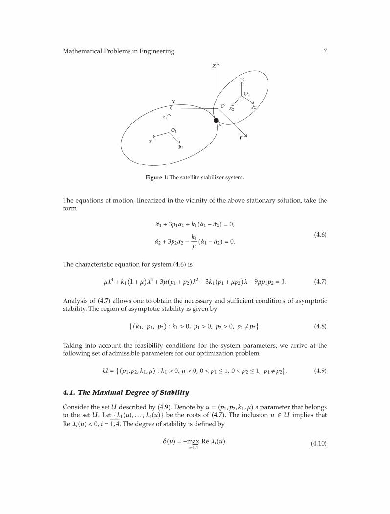
Consider motion of a connected two-body system in a circular orbit around the Earth. Body1 is a satellite with the center of mass O1, and body 2 is a stabilizer with the center of massO2 . These two bodies are linked to each other at the point P through a dissipative hingemechanism (Figure 1). LetO be the center of mass of the system.

We use three reference frames: OXYZ is the orbital coordinate frame, its axis OZis directed along the radius vector of the point O with respect to the center of the Earth,OX is directed along the velocity of the point O, and OY is normal to the orbit plane. Theaxes of referential frames O1x1y1z1 and O2x2y2z2 are the central principal axes of inertiafor bodies 1 and 2, respectively. Consider motion of the system in the orbit plane supposingthat the bodies are connected in their centres of mass; that is, the points O1, O2, O, and Pcoincide. Let α1 and α2 be the angles between the axis OX and the axes O1x1 and O2x2,respectively. Denote by α′

i, i = 1, 2 the derivative of αi with respect to time. The equations ofmotion for this system can be written as [6]

B1α′′1 + 3ω2

0(A1 − C1) sin α1 cosα1 + k1(

α′1 − α′

2)

= 0,

B2α′′2 + 3ω2

0(A2 − C2) sin α2 cosα2 − k1(

α′1 − α′

2)

= 0.(4.1)

Here, A1, B1, C1 and A2, B2, C2 are the principal moments of inertia of the bodies, k1 is thedamping coefficient of the system, and ω0 is the constant angular velocity of the orbitalmotion of the system’s center of mass. Introducing a new independent variable τ = ω0t andthe dimensionless parameters

p1 =A1 −C1

B1, p2 =

A2 − C2

B2, μ =

B2

B1, k1 =

k1

ω0B1, (4.2)

the equations of motion can be written as

α1 + 3p1 sinα1 cos α1 + k1(α1 − α2) = 0,

α2 + 3p2 sinα2 cosα2 − k1μ(α1 − α2) = 0.

(4.3)

Here, the dot denotes the derivative with respect to τ . The parameters (p1, p2, k1, μ) satisfythe following conditions:

−1 ≤ p1 ≤ 1, −1 ≤ p2 ≤ 1, μ > 0, k1 > 0. (4.4)

We study small oscillations of system (4.3) in the vicinity of the equilibrium position

α10 = 0, α20 = 0. (4.5)

Mathematical Problems in Engineering 7

X

Y

Z

x1

x2

y1

y2

z1

z2

O

PO1

O2

Figure 1: The satellite stabilizer system.

The equations of motion, linearized in the vicinity of the above stationary solution, take theform

α1 + 3p1α1 + k1(α1 − α2) = 0,

α2 + 3p2α2 − k1μ(α1 − α2) = 0.

(4.6)

The characteristic equation for system (4.6) is

μλ4 + k1(

1 + μ)

λ3 + 3μ(

p1 + p2)

λ2 + 3k1(

p1 + μp2)

λ + 9μp1p2 = 0. (4.7)

Analysis of (4.7) allows one to obtain the necessary and sufficient conditions of asymptoticstability. The region of asymptotic stability is given by

{(

k1, p1, p2)

: k1 > 0, p1 > 0, p2 > 0, p1 /= p2}

. (4.8)

Taking into account the feasibility conditions for the system parameters, we arrive at thefollowing set of admissible parameters for our optimization problem:

U ={(

p1, p2, k1, μ)

: k1 > 0, μ > 0, 0 < p1 ≤ 1, 0 < p2 ≤ 1, p1 /= p2}

. (4.9)

4.1. The Maximal Degree of Stability

Consider the set U described by (4.9). Denote by u = (p1, p2, k1, μ) a parameter that belongsto the set U. Let {λ1(u), . . . , λ4(u)} be the roots of (4.7). The inclusion u ∈ U implies thatRe λi(u) < 0, i = 1, 4. The degree of stability is defined by

δ(u) = −maxi=1,4

Re λi(u). (4.10)

8 Mathematical Problems in Engineering

Consider the following problem

δ(u) −→ max,

u ∈ U.(4.11)

In [7, 8], it is proved that the maximal degree of stability is achieved when all the roots of thecharacteristic equations are real and equal. This situation becomes possible only when theconditions

k1 = 4δ(u)μ

1 + μ,

p1 + p2 = 2δ2(u),

3(

p1 + μp2)

=(

1 + μ)

δ2(u),

9p1p2 = δ4(u)

(4.12)

are satisfied. The above system has two sets of solutions

p1 =(

3 − 2√2)2

� 0.0294,

p2 = 1,

k1 =√6(

3 − 2√2)

� 0.4203,

μ = 3 − 2√2 � 0.1716,

(4.13)

p1 = 1,

p2 =(

3 − 2√2)2 � 0.0294,

k1 =√6 � 2.4495,

μ = 3 + 2√2 � 5.8284.

(4.14)

4.2. Numerical Optimization

Denote by x(·, x0, p1, p2, k1, μ) the solution of linear system (4.6) with x(0) = x0, defined inthe interval [0, T]. The parameters (p1, p2, k1, μ)belong to asymptotic stability region defined

Mathematical Problems in Engineering 9

in (4.9). Consider the following problem:

max|x0|=1

∣∣x(

T, x0, p1, p2, k1, μ)∣∣ −→ min, k1 > 0, μ > 0, 0 < p1 ≤ 1, 0 < p2 ≤ 1. (4.15)

Problem (4.15) can be reduced to an optimization problemwithout constrains using quadraticpenalty functions; see [9]. If T is big enough, this problem approximates problem (4.11),where the concept of degree of stability is used. The parameters given by (4.13) and (4.14)are close to optimal solutions of problem (4.15) only when T � 1. Put T = 10π . The results ofsimulations show that the value of problem (4.15) is about 10−6–10−7, independently on thevalues of admissible parameters (p1, p2, k1, μ). For example, the following values

p1 = 0.0779, p2 = 0.8574, k1 = 0.5540, μ1 = 0.3337 (4.16)

are optimal parameters for problem (4.15). The corresponding minimal value is 7.2 × 10−7.Parameters (4.13) and (4.14) give the values 1.0 × 10−6 and 5.9 × 10−7, respectively.

In practice, it is important to consider smaller time intervals [0, T]. Solve problem(4.15) with T = 3π . In this case, we see that the value of problem really depends on thechoice of parameters. Let us estimate the global minimum in this problem. To this end, wesolve problem (4.15) using all combinations of the following values:

p1 = 0.25, 0.5, 0.75,

p2 = 0.25, 0.5, 0.75,

k1 = 1, 2, 3,

μ = 2, 4, 6,

(4.17)

as initial guesses for numerical optimization. We obtain the following two sets of parameterswith the best value of the problem:

p1 = 0.06928, p2 = 1.00757, k1 = 0.59209, μ = 0.33161, (4.18)

p1 = 1.00521, p2 = 0.06920, k1 = 1.78178, μ = 3.01152. (4.19)

The estimate for the global minimum m is

m = 0.00378. (4.20)

Meanwhile, the value corresponding to parameters (4.13) and (4.14) is 0.4660. Thus, we seethat the methodology based on resolution of problem (2.3) can be more adequate in thepractice than that one using the concept of degree of stability.

Since we are studying the behaviour of a nonlinear system in a vicinity of itsequilibrium position, it is also important to estimate the deviation of the linearized systemtrajectories from zero. The stabilizer constructed for the linearized systemmakes sense only ifits trajectories belong to a small vicinity of the equilibrium position; otherwise, the influence

10 Mathematical Problems in Engineering

of the nonlinearity can destabilize the system even in a very small neighbourhood of theequilibrium.

Consider the following problem:

maxt∈[0,3π]

max|x0|=1

∣∣x(

t, x0, p1, p2, k1, μ)∣∣ −→ min,

max| x0|=1

∣∣x(

3π, x0, p1, p2, k1, μ)∣∣ ≤ 0.005,

k1 > 0,

μ > 0,

0 < p1 ≤ 1,

0 < p2 ≤ 1.

(4.21)

In this problem, the solutions of system (4.6) at the moment T = 3π are constrained to be ina neighbourhood of the equilibrium position with the radius 0.005. The obtained optimalsolutions (p1, p2, k1, μ)minimize the maximum norm of the damping process of linear system(4.6) in the interval [0, 3π]. After numerical optimization, we get the following optimalparameters:

p1 = 0.07140, p2 = 1.01643, k1 = 0.60004, μ = 0.33887, (4.22)

p1 = 1.01642, p2 = 0.07140, k1 = 1.77067, μ = 2.95097. (4.23)

The corresponding value of problem (4.21) is P = 1.58685. We can see that the couple ofparameters in (4.22) and (4.23) are slightly different from (4.18) and (4.19). Moreover,

maxt∈[0,3π]

max|x0|=1

∣∣∣x(

t, x0, p1, p2, k1, μ)∣∣∣ � 1.5974 � P. (4.24)

Taking the optimal parameters (p1, p2, k1, μ) of problem (4.11), we get

maxt∈[0,3π]

max|x0|=1

∣∣∣x(

t, x0, p1, p2, k1, μ)∣∣∣ � 1.9169. (4.25)

Thus, the stabilizer with the parameters corresponding to the maximal degree of stabilityyields more significant deviation of the trajectories from the equilibrium position than thestabilizer with the parameters obtained solving problem (4.21).

Our aim is to find optimal parameters for system (4.3). To this end, we solve problem(4.15), with T = 3π , but now, x(·, x0, p1, p2, k1, μ) stands for the solution of system (4.3) withx(0) = x0. We get the following two sets of optimal parameters:

p1 = 0.23350, p2 = 1.08235, k1 = 0.62791, μ = 0.62137, (4.26)

p1 = 1.07743, p2 = 0.23171, k1 = 1.02413, μ = 1.63140. (4.27)

Mathematical Problems in Engineering 11

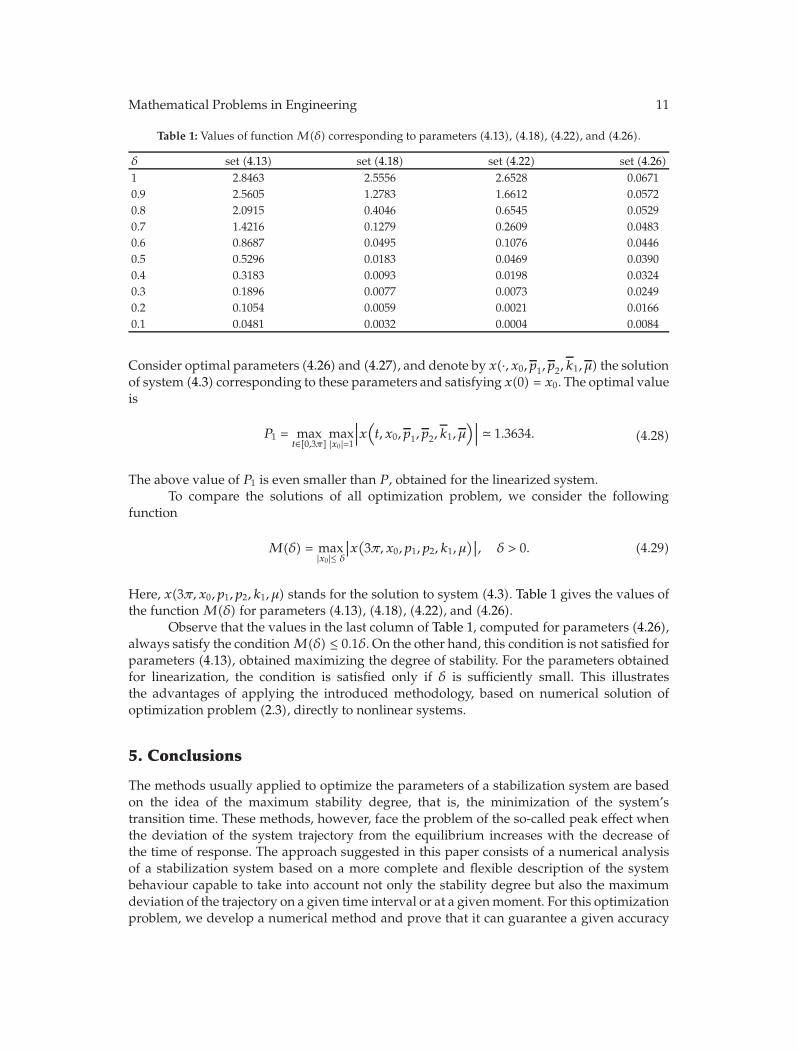
Table 1: Values of function M(δ) corresponding to parameters (4.13), (4.18), (4.22), and (4.26).

δ set (4.13) set (4.18) set (4.22) set (4.26)1 2.8463 2.5556 2.6528 0.06710.9 2.5605 1.2783 1.6612 0.05720.8 2.0915 0.4046 0.6545 0.05290.7 1.4216 0.1279 0.2609 0.04830.6 0.8687 0.0495 0.1076 0.04460.5 0.5296 0.0183 0.0469 0.03900.4 0.3183 0.0093 0.0198 0.03240.3 0.1896 0.0077 0.0073 0.02490.2 0.1054 0.0059 0.0021 0.01660.1 0.0481 0.0032 0.0004 0.0084

Consider optimal parameters (4.26) and (4.27), and denote by x(·, x0, p1, p2, k1, μ) the solutionof system (4.3) corresponding to these parameters and satisfying x(0) = x0. The optimal valueis

P1 = maxt∈[0,3π]

max|x0|=1

∣∣∣x(

t, x0, p1, p2, k1, μ)∣∣∣ � 1.3634. (4.28)

The above value of P1 is even smaller than P , obtained for the linearized system.To compare the solutions of all optimization problem, we consider the following

function

M(δ) = max|x0|≤ δ

∣∣x(

3π, x0, p1, p2, k1, μ)∣∣, δ > 0. (4.29)

Here, x(3π, x0, p1, p2, k1, μ) stands for the solution to system (4.3). Table 1 gives the values ofthe function M(δ) for parameters (4.13), (4.18), (4.22), and (4.26).

Observe that the values in the last column of Table 1, computed for parameters (4.26),always satisfy the conditionM(δ) ≤ 0.1δ. On the other hand, this condition is not satisfied forparameters (4.13), obtained maximizing the degree of stability. For the parameters obtainedfor linearization, the condition is satisfied only if δ is sufficiently small. This illustratesthe advantages of applying the introduced methodology, based on numerical solution ofoptimization problem (2.3), directly to nonlinear systems.

5. Conclusions

The methods usually applied to optimize the parameters of a stabilization system are basedon the idea of the maximum stability degree, that is, the minimization of the system’stransition time. These methods, however, face the problem of the so-called peak effect whenthe deviation of the system trajectory from the equilibrium increases with the decrease ofthe time of response. The approach suggested in this paper consists of a numerical analysisof a stabilization system based on a more complete and flexible description of the systembehaviour capable to take into account not only the stability degree but also the maximumdeviation of the trajectory on a given time interval or at a givenmoment. For this optimizationproblem, we develop a numerical method and prove that it can guarantee a given accuracy

12 Mathematical Problems in Engineering

for the problem solution. We obtained more precise estimates for the number of points inthe meshes needed to achieve a given discretization accuracy than the estimates based onthe usual Gronwall inequality. This method is applied to optimization of a stabilizationsystem for a satellite with a gravitational stabilizer. The obtained results show that the aboveapproach can offer solutions more adequate for practical implementation than those given byoptimization of the stability degree.

Appendix

A. The Mathematical Basis

In this Appendix, we present a series of theorems, with schematic proofs, containing explicitestimates for the fineness of discretization needed to obtain the necessary precision ofapproximations and to prove Theorem 3.1.

A.1. Linear Systems

Consider a linear system

x = Ax, x ∈ Rn, t ≥ 0, (A.1)

where A is a matrix. Assume that all its eigenvalues have negative real part. Let V be asymmetric positive definite matrix satisfying the Lyapunov equation [10]

A∗V + VA = −I. (A.2)

Set

P ={

p ∈ Rn | ⟨p, Vp⟩ ≤ 1

}

. (A.3)

The quadratic form V (p) = 〈p, Vp〉 is the Lyapunov function for system (A.1). Denote by η1

and η2 the minimal and maximal eigenvalues of V , respectively. Let τ be a positive constant.Consider the Euler approximation for system (A.1),

yk+1 = yk + τAyk, k = 0, 1, . . . . (A.4)

The following theorem provides an explicit estimate for the constant τ guaranteeing theequality limk→∞yk = 0.

Theorem A.1. Let b > 0. Consider y0 ∈ bP . If

0 < τ <η1

η22|A|2 , (A.5)

Mathematical Problems in Engineering 13

then the following inequalities hold:

⟨

yk, Vyk

⟩ ≤ βk⟨

y0, V y0⟩

, k = 1, 2, . . . , (A.6)

where

β = 1 − τ

η2+ τ2η2

η1|A|2. (A.7)

It is easy to see that 0 < β < 1. The proof of this theorem uses the induction and the inequality

η1∣∣p∣∣2 ≤ 〈p, Vp〉 ≤ η2

∣∣ p

∣∣2. (A.8)

Assume that constant τ satisfies condition (A.5). Consider the polygonal Euler approx-imation to solution of system (A.1)

y(t) = yk + (t − tk)Ayk, t ∈ [tk, tk+1],tk = kτ, k = 0, 1, . . . .

(A.9)

Let b > 0. Set

γ = − min〈p,Vp〉=1〈y,Vy〉≤ b2

〈A2y, Vp〉,(A.10)

ξμ(t) = ξ0e−μt, ξ0 > 0, (A.11)

x(t) = eAtx(0). (A.12)

Theorem A.2. Let y0 ∈ bP be given. Assume that condition 0 ≤ μ < 1/2η2 is satisfied. If

τγ ≤(

12η2

− μ

)

ξμ(t), t ≥ 0, (A.13)

then the inequality |y(t)− x(t)| ≤ ξμ(t)/√η1 holds for all t ∈ [0, T], whenever |y0 −x(0)| ≤ ξ0/

√η2.

This theorem is a consequence of the inequality

max〈p,Vp〉=1

⟨

Ap, Vp⟩ ≤ − 1

2η2, (A.14)

of the inclusion

1√η2

B ⊂ P ⊂ 1√η1

B, (A.15)

and of Theorem 3.2 with function y(·) defined by (A.9) and function ξ(·) defined by (A.11).The following theorem is also a consequence of Theorem 3.2.

14 Mathematical Problems in Engineering

TheoremA.3. Let x(t) = eAtx0 and z(t) = eAtz0 be solutions to system (A.1). Assume that x0, z0 ∈P . If

0 ≤ μ ≤ 12η2

, (A.16)

then the inequality |z(t) − x(t)| ≤ ξμ(t)/√η1, t ∈ [0, T] holds whenever |z0 − x0| ≤ ξ0/

√η2.

Consider now t ∈ Δ ⊂ [0, T], where Δ is a closed interval. Let x(t, x0) be the solutionof system (A.1), with

x0 ∈ S = {x ∈ Rn : |x| = 1}. (A.17)

Let δ > 0. Assume that parameters of function ξμ(·) defined by (A.11) satisfy the followingconditions,

ξ0 =√η2δ, 0 ≤ μ <

12η2

. (A.18)

Assume that {xj}, j = 1, J is a finite set of points uniformly distributed on S. If

J ≥ 2([

1δ

]

+ 1)n−1

, (A.19)

then we have

J⋃

j=1

(

xj + δB) ⊃ S. (A.20)

Let |Δ| be the length of the interval Δ. Consider a finite set {tk} ⊂ Δ, k = 0,N, such that thedifference

tk+1 − tk = τ =δ

2γ√η2(A.21)

is a constant. If

N =[2γ√η2

δ|Δ|

]

+ 1, (A.22)

then the set

N⋃

k=0

[

tk − δ

4γ√η2, tk +

δ

4γ√η2

]

(A.23)

Mathematical Problems in Engineering 15

contains Δ. Consider the Euler approximation of solution x(t, x0)

x(

tk+1, xj

)

= x(

tk, xj

)

+ τAx(

tk, xj

)

, k = 0,N. (A.24)

Theorem A.4. Let ε > 0. If

δ =4γ√η1

8γ√η2 + |A|ε, (A.25)

then the following inequality holds:

∣∣∣∣∣maxk=0,N

maxj=1,J

∣∣ x

(

tk, xj

)∣∣ −max

t∈Δmaxx0∈S

|x(t, x0)|∣∣∣∣∣≤ ε. (A.26)

The proof of this theorem uses the results of Theorems A.1, A.2, and A.3.

A.2. Nonlinear Systems

Assume that g : Rn → Rn is a twice continuously differentiable function satisfying g(0) = 0.Consider the function f(x) = Ax + g(x), whereA is a matrix. Assume that the eigenvalues ofthe matrix A have negative real parts. Consider the system

x = f(x), t ≥ 0. (A.27)

Since g is twice continuously differentiable, there exists a constant Lg > 0 such that functiong(·) satisfies the following Lipschitz condition:

∣∣g(x1) − g(x2)

∣∣ ≤ Lg max{|x1|, |x2|}|x1 − x2|, (A.28)

for all x1 and x2 in a small neighbourhood of the equilibrium position x = 0. Consider the setP defined by (A.3) and constants η1, η2 as before. Define the Euler approximation for system(A.27),

yk+1 = yk + τf(

yk

)

, k = 0, 1, . . . , (A.29)

where τ is a positive constant.

Theorem A.5. Assume that b is a constant satisfying

0 < b <

√η1

4Lgη2. (A.30)

16 Mathematical Problems in Engineering

Let y0 ∈ bP . If

0 < τ <8η2

1

η2(

4|A|η2 + 1)2 , (A.31)

then the following inequalities hold:

⟨

yk, Vyk

⟩ ≤ βk⟨

y0, V y0⟩

, k = 1, 2 . . . , (A.32)

where

β = 1 − τ

2η2+ τ2

(

4|A|η2 + 1)2

16η21

. (A.33)

The proof of this theorem uses the Lipschitz condition (A.28) in the form

∣∣g(

yk

)∣∣ ≤ Lg

∣∣yk

∣∣2, (A.34)

and the mathematical induction method. It is easy to see that 0 < β < 1.Assume that the constant τ satisfies condition (A.31) and consider the function

y(t) = yk + (t − tk)f(

yk

)

, t ∈ [tk, tk+1], tk = kτ, k = 0, 1, . . . . (A.35)

Put

γ1 = γ +8η2|A| + 1

64η22√η1Lg

, (A.36)

where γ is defined by (A.10). Denote by x(t) the solution to system (A.27) with the initialcondition x(0) = x0.

Theorem A.6. Assume that b is a constant satisfying

ξ0 ≤ b ≤√η1

4Lgη2, (A.37)

and let y0 ∈ bP . If 0 ≤ μ < 1/4η2 and

τγ1 ≤(

14η2

− μ

)

ξμ(t), t ≥ 0, (A.38)

then the inequality |y(t)− x(t)| ≤ ξμ(t)/√η1 holds for all t ∈ [0, T], whenever |y0 −x(0)| ≤ ξ0/

√η2.

Mathematical Problems in Engineering 17

This theorem is a consequence of Theorem 3.2 with function y(·) defined by (A.35)and function ξ(·) defined by (A.11).

Consider now the Cauchy problems

x = f(x),

x(0) = x0,

z = f(z),

z(0) = z0.

(A.39)

Denote by x(·) and z(·) the respective solutions. The following theorem is also aconsequence of Theorem 3.2.

Theorem A.7. Let b be a constant satisfying

ξ0 ≤ b ≤√η1

4Lgη2. (A.40)

Assume that the trajectories x(·) and z(·) belong to the set bP . If

0 ≤ μ ≤ 14η2

, (A.41)

then we have |z(t) − x(t)| ≤ ξμ(t)/√η1 for all t ∈ [0, T], whenever |z0 − x0| ≤ ξ0/

√η2.

Let δ > 0. Assume that the parameters of function ξμ(·) defined by (A.11) satisfy thefollowing conditions:

ξ0 =√η2δ, 0 ≤ μ ≤ 1

4η2. (A.42)

Consider the balls

Bbi =

{

x ∈ Rn : |x| ≤ bi√η2

}

⊂ biP, i = 0, m, (A.43)

where the constants bi satisfy the following conditions:

ξ0 ≤ bi ≤√η1

4Lgη2, i = 0, m. (A.44)

18 Mathematical Problems in Engineering

For each index i, take a finite set {xij} of points, j = 1, Ji, uniformly distributed in the ball Bbi .

If

Ji ≥([

bi√η2δ

]

+ 1

)n

, (A.45)

then we have

Ji⋃

j=1

(

xij + δB

)

⊃ Bbi. (A.46)

Let Δi ⊂ [0, T], i = 0, m, be closed intervals with length |Δi|. Consider a finite set of points{ti

k}, k = 0,Ni, in each interval Δi. It is assumed that the difference τ = ti

k+1 − tikis a constant.

Let

τ =δ

4γ1√η2

. (A.47)

Define the sets

ΔNi =Ni⋃

k=0

[

tik −δ

8γ1√η2

, tik +δ

8γ1√η2

]

, i = 0, m. (A.48)

If

Ni =[4γ1

√η2

δ|Δi|

]

+ 1, (A.49)

then we have ΔNi ⊃ Δi. Let x0 ∈ Bbi . Denote by x(t, x0) the solution to the Cauchy problem

x = Ax + g(x), x ∈ Rn, t ∈ Δi,

x(0) = x0.(A.50)

Consider the Euler approximation of the solution x(t, x0)

x(

tik+1, xij

)

= x(

tik, xij

)

+ τ[

Ax(

tik, xij

)

+ g(

x(

tik, xij

))]

, k = 0,Ni, (A.51)

with τ satisfying condition (A.47).

Theorem A.8. Let ε > 0 be given. If

δ =27Lgγ1η

22√η1η2

28Lgγ1η32 + 4η2

√η1|A| +√

η1ε, (A.52)

Mathematical Problems in Engineering 19

then the following inequalities:

∣∣∣∣∣maxk=0,Ni

maxj=1,Ji

∣∣∣x(

tik, xij

)∣∣∣ −max

t∈Δi

maxx0∈Bbi

|x(t, x0)|∣∣∣∣∣≤ ε, i = 0, m, (A.53)

hold.

The proof of this theorem follows from Theorems A.5, A.6, and A.7.

Acknowledgments

The authors are grateful to the reviewers for their valuable suggestions. This research issupported by the Portuguese Foundation for Science and Technologies (FCT), the PortugueseOperational Programme for Competitiveness Factors (COMPETE), the Portuguese StrategicReference Framework (QREN), and the European Regional Development Fund (FEDER).

References

[1] R. N. Ismailov, “The peack effect in stationary linear systems with scalar inputs and outputs,”Automation and Remote Control, vol. 48, no. 8, part 1, pp. 1018–1024, 1987.

[2] H. J. Sussmann and P. V. Kokotovic, “The peaking phenomenon and the global stabilization ofnonlinear systems,” IEEE Transactions on Automatic Control, vol. 36, no. 4, pp. 424–440, 1991.

[3] Ya. Z. Cypkin and P. V. Bromberg, “On the degree of stability of linear systems,” USSR Academy ofSciences, Branch of Technical Sciences, vol. 1945, no. 12, pp. 1163–1168, 1945.

[4] F. H. Clarke, Optimization and Nonsmooth Analysis, Canadian Mathematical Society Series ofMonographs and Advanced Texts, John Wiley & Sons, New York, NY, USA, 1983.

[5] G. Smirnov and F. Miranda, “Filippov-Gronwall inequality for discontinuous differential inclusions,”International Journal of Mathematics and Statistics, vol. 5, no. A09, pp. 110–120, 2009.

[6] V. A. Sarychev, “Investigation of the dynamics of a gravitational stabilization system,” in XIIIthInternational Astronautical Congress, pp. 658–690, Varna, Bulgaria, 1964.

[7] R. L. Borrelli and I. P. Leliakov, “An optimization technique for the transient response of passivelystable satellites,” Journal of Optimization Theory and Applications, vol. 10, pp. 344–361, 1972.

[8] V. A. Sarychev and V. V. Sazonov, “Optimal parameters of passive systems for satellite orientation,”Cosmic Research, vol. 14, no. 2, pp. 183–193, 1976.

[9] R. Fletcher, Practical Methods of Optimization, John Wiley & Sons, Chichester, UK, 2nd edition, 1987.[10] A. M. Liapunov, Stability of Motion, Academic Press, New York, NY, USA, 1966.