Optimization of Offshore Wind Farm Installation Procedure With a Targeted Finish Date Vigney Kumar Delft University of Technology

Welcome message from author
This document is posted to help you gain knowledge. Please leave a comment to let me know what you think about it! Share it to your friends and learn new things together.
Transcript
Optimization of Offshore WindFarm Installation ProcedureWith a Targeted Finish Date
Vigney Kumar
DelftUniversityofTechnology


Optimization of Offshore Wind FarmInstallation Procedure With a Targeted Finish
Date
by
Vigney Kumar
in partial fulfillment of the requirements for the degree of
Master of Science
in Sustainable Energy Technology
at the Delft University of Technology,
to be defended publicly on Friday November 24, 2017.
Thesis committee: Prof. dr. S. J. Watson, TU Delft, Chair of the thesis committeeDr. ir. M. B. Zaayer, TU Delft, Supervisorir. Ashish Dewan , ECN, SupervisorDr. ir. O. M. Napoles, TU Delft, External
An electronic version of this thesis is available at http://repository.tudelft.nl/.


Abstract
Offshore Wind Farm (OWF) installation procedure is a complicated phase requiring excellent manage-ment of resources for timely completion of tasks. As installation cost is an important aspect of thebuilding phase of the OWF, the graduation project looks into the optimization of offshore wind farminstallation procedure with a targeted completion date as a priority. In this thesis, an optimizationapproach is built around an ECN in-house software, specially developed for simulating various OWFinstallation strategies. Ultimately, the result of the dissertation is to have a method that providesadded flexibility to simulate different OWF installation planning, yet obtaining optimal installation cost.A concise literature review describes the significance of the current research and the potential thatmetaheuristic approaches bring to solve installation scheduling problems. Within the metaheuristicapproach, the genetic algorithm is chosen as the optimization procedure to use in current work. Theobjective of the optimization procedure throughout the research is minimizing the total installationcost. The target end date in this study is implemented in the form of a constraint to steer the opti-mizer solution within the specified limit. A new methodology is proposed to generate an automatedplanning for the different installation procedures to facilitate the link between the optimizer and ECNtool. The project also considers uncertainty introduced due to weather and describes the considera-tions made to account for the same. The different case-studies illustrate the potential of introducinga metaheuristic optimizer in solving OWF installation scheduling problems. While, the new procedureleads to obtaining reduced installation costs for a given planning, analyzing with real OWF projects willfurther substantiate the chosen approach.
iii


Acknowledgement
I wish to thank some important people who helped me bring this thesis work to a good end. Firstly, Iwould like to express thanks to Prof. Michiel Zaaijer for helping me find a topic that suited my curiosity.I consider myself fortunate to have you as my supervisor, without your attention, enthusiasm andguidance, my work would not have been productive.
To Georgios Katsouris and Ashish Dewan, I am grateful for allowing me to work on a challengingand relevant topic as an intern at ECN. A special appreciation for Ashish for his selfless support andassistance during the complete project period. I am very thankful to Clym Stock-Williams for hissupport and assistance with helping me understand and implementing the optimization procedure.Furthermore, I am grateful to Piet Warnaar from ECN for his valuable inputs and suggestions duringthe modeling process of the project. Moreover, a big thanks to all my friends and colleagues at ECNfor making my stay even more special.
I am thankful towards the complete examination committee for the time spent on evaluating thisdocument. Last but not least, I would like to thank my family and friends for supporting me in this laststage of my study.
Vigney KumarDelft, November 2017
v


Contents
List of Figures ix
List of Tables xi
1 Introduction 11.1 Research Motivation . . . . . . . . . . . . . . . . . . . . . . . . . . . . . . . . . . . . . 21.2 Objective . . . . . . . . . . . . . . . . . . . . . . . . . . . . . . . . . . . . . . . . . . . . 41.3 Report Outline . . . . . . . . . . . . . . . . . . . . . . . . . . . . . . . . . . . . . . . . 4
2 Offshore Installation Scheduling Problem 52.1 Offshore Wind Installation Challenges . . . . . . . . . . . . . . . . . . . . . . . . . . 5
2.1.1 Foundations. . . . . . . . . . . . . . . . . . . . . . . . . . . . . . . . . . . . . . 52.1.2 Wind Turbines . . . . . . . . . . . . . . . . . . . . . . . . . . . . . . . . . . . . 62.1.3 Cables . . . . . . . . . . . . . . . . . . . . . . . . . . . . . . . . . . . . . . . . . 62.1.4 Conclusion . . . . . . . . . . . . . . . . . . . . . . . . . . . . . . . . . . . . . . 6
2.2 ECN Install . . . . . . . . . . . . . . . . . . . . . . . . . . . . . . . . . . . . . . . . . . 72.3 Optimization of Installation Planning . . . . . . . . . . . . . . . . . . . . . . . . . . . 7
2.3.1 Need for Optimization . . . . . . . . . . . . . . . . . . . . . . . . . . . . . . . . 82.3.2 Existing Studies on OWF Installation and Planning . . . . . . . . . . . . . . 82.3.3 Optimization Choices . . . . . . . . . . . . . . . . . . . . . . . . . . . . . . . . 9
2.4 Optimizer Addition to ECN Install . . . . . . . . . . . . . . . . . . . . . . . . . . . . . 10
3 Automated Planning 133.1 Automated Planning Requirement. . . . . . . . . . . . . . . . . . . . . . . . . . . . . 133.2 Automated Planning Blocks . . . . . . . . . . . . . . . . . . . . . . . . . . . . . . . . 133.3 AP Block Inputs. . . . . . . . . . . . . . . . . . . . . . . . . . . . . . . . . . . . . . . . 14
3.3.1 Vessel Type Library . . . . . . . . . . . . . . . . . . . . . . . . . . . . . . . . . 153.3.2 Harbor Library . . . . . . . . . . . . . . . . . . . . . . . . . . . . . . . . . . . . 163.3.3 Equipment Library . . . . . . . . . . . . . . . . . . . . . . . . . . . . . . . . . . 173.3.4 Default Database Template . . . . . . . . . . . . . . . . . . . . . . . . . . . . . 17
3.4 AP block implementation . . . . . . . . . . . . . . . . . . . . . . . . . . . . . . . . . . 173.5 Interdependency between Sequences . . . . . . . . . . . . . . . . . . . . . . . . . . . 213.6 Automated Planning Integration with Optimizer . . . . . . . . . . . . . . . . . . . . 233.7 AP Block Verification. . . . . . . . . . . . . . . . . . . . . . . . . . . . . . . . . . . . . 24
4 Optimizer Modelling 274.1 Optimization Model Setup . . . . . . . . . . . . . . . . . . . . . . . . . . . . . . . . . 27
4.1.1 Installation Problem Design Variables . . . . . . . . . . . . . . . . . . . . . . 284.1.2 Objective Function . . . . . . . . . . . . . . . . . . . . . . . . . . . . . . . . . . 284.1.3 Constraints . . . . . . . . . . . . . . . . . . . . . . . . . . . . . . . . . . . . . . 29
4.2 Uncertainty Consideration . . . . . . . . . . . . . . . . . . . . . . . . . . . . . . . . . 304.2.1 Weather Simulation Requirements . . . . . . . . . . . . . . . . . . . . . . . . 304.2.2 ECN Install Output Analysis . . . . . . . . . . . . . . . . . . . . . . . . . . . . 31
4.3 Genetic Algorithm . . . . . . . . . . . . . . . . . . . . . . . . . . . . . . . . . . . . . . 324.3.1 Genetic Algorithm Terminology . . . . . . . . . . . . . . . . . . . . . . . . . . 324.3.2 Genetic Algorithm Operation . . . . . . . . . . . . . . . . . . . . . . . . . . . . 344.3.3 MATLAB GA Integer Solver . . . . . . . . . . . . . . . . . . . . . . . . . . . . . 36
4.4 GA Parameter Tuning . . . . . . . . . . . . . . . . . . . . . . . . . . . . . . . . . . . . 374.4.1 Abstract Problem . . . . . . . . . . . . . . . . . . . . . . . . . . . . . . . . . . . 374.4.2 Control Parameter Testing . . . . . . . . . . . . . . . . . . . . . . . . . . . . . 394.4.3 Conclusion . . . . . . . . . . . . . . . . . . . . . . . . . . . . . . . . . . . . . . 40
vii

viii Contents
5 Case Study 435.1 OWF location . . . . . . . . . . . . . . . . . . . . . . . . . . . . . . . . . . . . . . . . . 435.2 Market Overview . . . . . . . . . . . . . . . . . . . . . . . . . . . . . . . . . . . . . . . 445.3 Case Study 1 . . . . . . . . . . . . . . . . . . . . . . . . . . . . . . . . . . . . . . . . . 44
5.3.1 Description . . . . . . . . . . . . . . . . . . . . . . . . . . . . . . . . . . . . . . 445.3.2 CASE 1A . . . . . . . . . . . . . . . . . . . . . . . . . . . . . . . . . . . . . . . . 455.3.3 CASE 1B . . . . . . . . . . . . . . . . . . . . . . . . . . . . . . . . . . . . . . . . 465.3.4 CASE 1C . . . . . . . . . . . . . . . . . . . . . . . . . . . . . . . . . . . . . . . . 475.3.5 Discussion. . . . . . . . . . . . . . . . . . . . . . . . . . . . . . . . . . . . . . . 49
5.4 Case Study 2 . . . . . . . . . . . . . . . . . . . . . . . . . . . . . . . . . . . . . . . . . 495.4.1 Description . . . . . . . . . . . . . . . . . . . . . . . . . . . . . . . . . . . . . . 495.4.2 Discussion. . . . . . . . . . . . . . . . . . . . . . . . . . . . . . . . . . . . . . . 53
6 Conclusions and Future Work 556.1 Conclusions . . . . . . . . . . . . . . . . . . . . . . . . . . . . . . . . . . . . . . . . . . 556.2 Future work . . . . . . . . . . . . . . . . . . . . . . . . . . . . . . . . . . . . . . . . . . 56
A Appendix A 59A.1 Wind Turbine components and Resources . . . . . . . . . . . . . . . . . . . . . . . . 59
A.1.1 Substructure . . . . . . . . . . . . . . . . . . . . . . . . . . . . . . . . . . . . . 59A.1.2 Wind Turbine Components . . . . . . . . . . . . . . . . . . . . . . . . . . . . . 60A.1.3 Electrical Infrastructure. . . . . . . . . . . . . . . . . . . . . . . . . . . . . . . 61A.1.4 Substation . . . . . . . . . . . . . . . . . . . . . . . . . . . . . . . . . . . . . . . 61A.1.5 Vessels . . . . . . . . . . . . . . . . . . . . . . . . . . . . . . . . . . . . . . . . . 62A.1.6 Equipment. . . . . . . . . . . . . . . . . . . . . . . . . . . . . . . . . . . . . . . 62A.1.7 Port . . . . . . . . . . . . . . . . . . . . . . . . . . . . . . . . . . . . . . . . . . . 64A.1.8 Working Technicians. . . . . . . . . . . . . . . . . . . . . . . . . . . . . . . . . 64
B Appendix B 65B.0.1 Inputs and Planning . . . . . . . . . . . . . . . . . . . . . . . . . . . . . . . . . 65B.0.2 Pre-Processor . . . . . . . . . . . . . . . . . . . . . . . . . . . . . . . . . . . . . 66B.0.3 Simulator . . . . . . . . . . . . . . . . . . . . . . . . . . . . . . . . . . . . . . . 66B.0.4 Post-Processor . . . . . . . . . . . . . . . . . . . . . . . . . . . . . . . . . . . . 67B.0.5 Install Model . . . . . . . . . . . . . . . . . . . . . . . . . . . . . . . . . . . . . 67
C Appendix C 69C.1 Data handling in ECN INSTALL . . . . . . . . . . . . . . . . . . . . . . . . . . . . . . 69C.2 Simulation settings for ECN Install . . . . . . . . . . . . . . . . . . . . . . . . . . . . 70
Bibliography 73
List of Figures
1.1 Offshore wind Energy Statistics [1] . . . . . . . . . . . . . . . . . . . . . . . . . . . . . 11.2 ECN Install User Interface . . . . . . . . . . . . . . . . . . . . . . . . . . . . . . . . . . 21.3 Capital cost breakup of an offshore wind turbine [2] . . . . . . . . . . . . . . . . . . . 3
2.1 ECN Install tool architecture . . . . . . . . . . . . . . . . . . . . . . . . . . . . . . . . 82.2 New project architecture . . . . . . . . . . . . . . . . . . . . . . . . . . . . . . . . . . 11
3.1 Automated planning flow diagram . . . . . . . . . . . . . . . . . . . . . . . . . . . . . 143.2 Sequence limitations . . . . . . . . . . . . . . . . . . . . . . . . . . . . . . . . . . . . 153.3 Vessel Library . . . . . . . . . . . . . . . . . . . . . . . . . . . . . . . . . . . . . . . . 163.4 Foundation transport methods . . . . . . . . . . . . . . . . . . . . . . . . . . . . . . . 183.5 Pre-assembly combinations [3] . . . . . . . . . . . . . . . . . . . . . . . . . . . . . . . 203.6 Pre-assembly Concepts applied in the industry . . . . . . . . . . . . . . . . . . . . . . 223.7 Interdependency between different sequences . . . . . . . . . . . . . . . . . . . . . . 233.8 Interdependency with multiple vessels . . . . . . . . . . . . . . . . . . . . . . . . . . . 233.9 AP block in Project architecture . . . . . . . . . . . . . . . . . . . . . . . . . . . . . . . 243.10 Installation planning simulated in ECN Install old (v2.1) . . . . . . . . . . . . . . . . . 253.11 Automated planning testing blocks . . . . . . . . . . . . . . . . . . . . . . . . . . . . . 25
4.1 Different end date exceeding penalty functions . . . . . . . . . . . . . . . . . . . . . . 294.2 ECN Install output uncertainty handling . . . . . . . . . . . . . . . . . . . . . . . . . . 314.3 GA terminology . . . . . . . . . . . . . . . . . . . . . . . . . . . . . . . . . . . . . . . 324.4 single point crossover operation . . . . . . . . . . . . . . . . . . . . . . . . . . . . . . 334.5 Mutation operation . . . . . . . . . . . . . . . . . . . . . . . . . . . . . . . . . . . . . 344.6 Different offspring for new population [4] . . . . . . . . . . . . . . . . . . . . . . . . . 344.7 GA work flow diagram . . . . . . . . . . . . . . . . . . . . . . . . . . . . . . . . . . . . 354.8 Design variable (DV) representation in GA population . . . . . . . . . . . . . . . . . . . 364.9 Knapsack problem representation in GA . . . . . . . . . . . . . . . . . . . . . . . . . . 384.10 Influence of crossover fraction . . . . . . . . . . . . . . . . . . . . . . . . . . . . . . . 404.11 Influence of elite count . . . . . . . . . . . . . . . . . . . . . . . . . . . . . . . . . . . 41
5.1 Borssele wind farm zone [5] . . . . . . . . . . . . . . . . . . . . . . . . . . . . . . . . 435.2 start date vs total installation cost . . . . . . . . . . . . . . . . . . . . . . . . . . . . . 465.3 Vessel types vs total installation cost . . . . . . . . . . . . . . . . . . . . . . . . . . . . 465.4 start date vs total installation cost . . . . . . . . . . . . . . . . . . . . . . . . . . . . . 475.5 Target end date comparison . . . . . . . . . . . . . . . . . . . . . . . . . . . . . . . . 485.6 Division 1 vs Division 2 Jack-up vessels . . . . . . . . . . . . . . . . . . . . . . . . . . 485.7 GA convergence plot . . . . . . . . . . . . . . . . . . . . . . . . . . . . . . . . . . . . 495.8 Sequence of installation activities . . . . . . . . . . . . . . . . . . . . . . . . . . . . . . 505.9 Sub-case start date ranges vs Installation costs . . . . . . . . . . . . . . . . . . . . . . 54
A.1 Types of substructures [3] . . . . . . . . . . . . . . . . . . . . . . . . . . . . . . . . . 59A.2 Wind turbine components:(a) Nacelle & Hub, (b) Blades, (c) Tower, (d) Tower section . 61A.3 Electrical infrastructure . . . . . . . . . . . . . . . . . . . . . . . . . . . . . . . . . . . 62A.4 Offshore substation . . . . . . . . . . . . . . . . . . . . . . . . . . . . . . . . . . . . . 62A.5 (a) Rock dumping vessel,(b) Heavy lift vessel,(c) Multi-purpose vessel,(d) Cable lay vessel 63A.6 (a) ROV ,(b) Pile hammer,(c) Crane . . . . . . . . . . . . . . . . . . . . . . . . . . . . 63A.7 Harbour use for OWWF installation . . . . . . . . . . . . . . . . . . . . . . . . . . . . . 64
B.1 Foundations installation planning . . . . . . . . . . . . . . . . . . . . . . . . . . . . . . 66
ix

x List of Figures
B.2 Pre-Processor planning gantt chart . . . . . . . . . . . . . . . . . . . . . . . . . . . . . 66B.3 Post-Process gantt chart . . . . . . . . . . . . . . . . . . . . . . . . . . . . . . . . . . 67B.4 Average delays breakdown per step and delay type. . . . . . . . . . . . . . . . . . . . 67
C.1 Database template structure . . . . . . . . . . . . . . . . . . . . . . . . . . . . . . . . 69C.2 Activity levels defined in ECN Install . . . . . . . . . . . . . . . . . . . . . . . . . . . . 70C.3 Planning data flow diagram to ECN Install . . . . . . . . . . . . . . . . . . . . . . . . . 70C.4 Settings file in ECN Install . . . . . . . . . . . . . . . . . . . . . . . . . . . . . . . . . . 71

List of Tables
3.1 Project inputs . . . . . . . . . . . . . . . . . . . . . . . . . . . . . . . . . . . . . . . . 153.2 Vessel Library . . . . . . . . . . . . . . . . . . . . . . . . . . . . . . . . . . . . . . . . 163.3 Verification sequence inputs . . . . . . . . . . . . . . . . . . . . . . . . . . . . . . . . 243.4 ECN Install old (v2.1) vs ECN Install (2.2) results . . . . . . . . . . . . . . . . . . . . . 263.5 Final verification . . . . . . . . . . . . . . . . . . . . . . . . . . . . . . . . . . . . . . . 26
4.1 Design variable bounds . . . . . . . . . . . . . . . . . . . . . . . . . . . . . . . . . . . 284.2 Optimization time vs Number of weather simulations . . . . . . . . . . . . . . . . . . . 314.3 Tuning parameters for GA . . . . . . . . . . . . . . . . . . . . . . . . . . . . . . . . . . 374.4 Problem similarity . . . . . . . . . . . . . . . . . . . . . . . . . . . . . . . . . . . . . . 394.5 Parameter tuning results . . . . . . . . . . . . . . . . . . . . . . . . . . . . . . . . . . 39
5.1 New projects in Europe region [6] . . . . . . . . . . . . . . . . . . . . . . . . . . . . . 445.2 Sub-cases for foundation installation . . . . . . . . . . . . . . . . . . . . . . . . . . . . 455.3 Optimization parameter specifications . . . . . . . . . . . . . . . . . . . . . . . . . . . 455.4 Optimal solution for sub-case 1A . . . . . . . . . . . . . . . . . . . . . . . . . . . . . . 455.5 Optimal solution for sub-case 1B . . . . . . . . . . . . . . . . . . . . . . . . . . . . . . 465.6 Optimal solution for sub-case 1C . . . . . . . . . . . . . . . . . . . . . . . . . . . . . . 495.7 Optimization parameters . . . . . . . . . . . . . . . . . . . . . . . . . . . . . . . . . . 505.8 Number of vessels and Pre-assembly combination design variable study . . . . . . . . . 515.9 Number of foundation vessel evaluation . . . . . . . . . . . . . . . . . . . . . . . . . . 515.10 Wind turbine preassembly combination evaluation . . . . . . . . . . . . . . . . . . . . 52
B.1 ECN Install Input parameters . . . . . . . . . . . . . . . . . . . . . . . . . . . . . . . . 65
xi


Nomenclature
Latin Symbols
𝐶 Total installation cost (€)
𝑐 Cost (€)
𝑑 Installation duration (days)
𝑓 Finish date
𝑗 Number of object types
𝑘 Object type
𝑛𝑠𝑖𝑚 Total number of weather realizations
𝑛𝑣𝑎𝑟𝑠 Number of variables
𝑂 Example objective function
𝑝() Penalty function
𝑣 Option cost per object (€)
𝑊 Knapsack weight limit
𝑤 Option weight per object (kg)
𝑥 Design variable
𝑦 Mean installation cost (€)
𝑦 Knapsack objective value
𝑌 Objective value (€)
Abbreviations
𝐴𝐵𝐶 Artificial Bee Colony
𝐴𝑃 Automated Planning
𝐵𝑊𝐹𝑍 Borssele Wind Farm Zone
𝐶𝐴𝑃𝐸𝑋 Capital Expenditure
𝐶𝐸 Constraint Evaluation
𝐷𝐸𝑆 Discrete Event Simulation
𝐸𝐶𝑁 Energy Research Centre of the Netherlands
𝐸𝐸𝑍 Exclusive Economic Zone
xiii

xiv List of Tables
𝐸𝑆 Evolutionary Strategy
𝐺𝐴 Genetic Algorithm
𝐺𝑈𝐼 Graphical User Interface
𝐼𝑃 Initial Planning
𝑀𝐼𝐿𝑃 Mixed Integer Linear Programming
𝑂 Optimizer
𝑂𝐻𝑉𝑆 Offshore High Voltage Station
𝑂𝑊𝐹 Offshore Wind Farm
𝑃𝑆𝑂 Particle Swarm Optimization
𝑅𝑂𝑉 Remotely Operated Underwater Vehicle
𝑆𝐴 Simulated Annealing
𝑆𝐷 Start Date
𝑇𝐸𝐷 Target End Date
𝑇𝑆𝑂 Transmission System Operator
𝑈𝐶 Uncertainty Consideration
𝑊𝑇 Wind Turbine
1Introduction
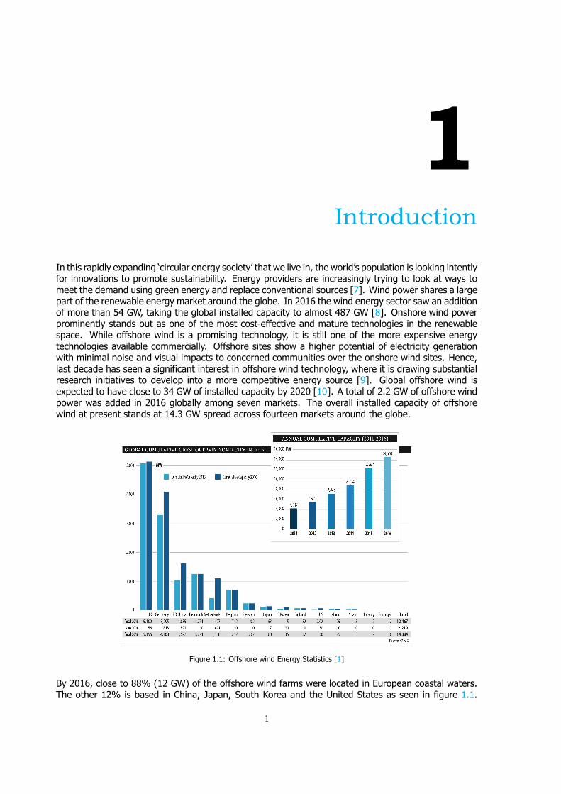
In this rapidly expanding ‘circular energy society’ that we live in, the world’s population is looking intentlyfor innovations to promote sustainability. Energy providers are increasingly trying to look at ways tomeet the demand using green energy and replace conventional sources [7]. Wind power shares a largepart of the renewable energy market around the globe. In 2016 the wind energy sector saw an additionof more than 54 GW, taking the global installed capacity to almost 487 GW [8]. Onshore wind powerprominently stands out as one of the most cost-effective and mature technologies in the renewablespace. While offshore wind is a promising technology, it is still one of the more expensive energytechnologies available commercially. Offshore sites show a higher potential of electricity generationwith minimal noise and visual impacts to concerned communities over the onshore wind sites. Hence,last decade has seen a significant interest in offshore wind technology, where it is drawing substantialresearch initiatives to develop into a more competitive energy source [9]. Global offshore wind isexpected to have close to 34 GW of installed capacity by 2020 [10]. A total of 2.2 GW of offshore windpower was added in 2016 globally among seven markets. The overall installed capacity of offshorewind at present stands at 14.3 GW spread across fourteen markets around the globe.
Figure 1.1: Offshore wind Energy Statistics [1]
By 2016, close to 88% (12 GW) of the offshore wind farms were located in European coastal waters.The other 12% is based in China, Japan, South Korea and the United States as seen in figure 1.1.
1
2 1. Introduction
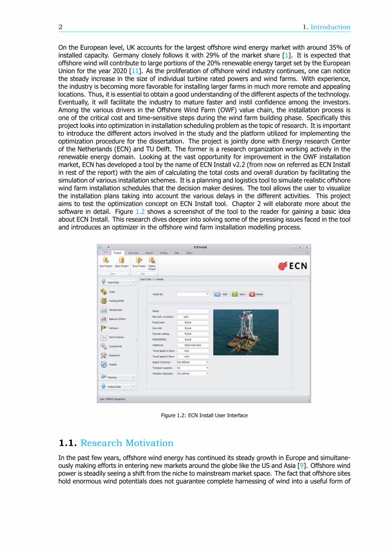
On the European level, UK accounts for the largest offshore wind energy market with around 35% ofinstalled capacity. Germany closely follows it with 29% of the market share [1]. It is expected thatoffshore wind will contribute to large portions of the 20% renewable energy target set by the EuropeanUnion for the year 2020 [11]. As the proliferation of offshore wind industry continues, one can noticethe steady increase in the size of individual turbine rated powers and wind farms. With experience,the industry is becoming more favorable for installing larger farms in much more remote and appealinglocations. Thus, it is essential to obtain a good understanding of the different aspects of the technology.Eventually, it will facilitate the industry to mature faster and instil confidence among the investors.Among the various drivers in the Offshore Wind Farm (OWF) value chain, the installation process isone of the critical cost and time-sensitive steps during the wind farm building phase. Specifically thisproject looks into optimization in installation scheduling problem as the topic of research. It is importantto introduce the different actors involved in the study and the platform utilized for implementing theoptimization procedure for the dissertation. The project is jointly done with Energy research Centerof the Netherlands (ECN) and TU Delft. The former is a research organization working actively in therenewable energy domain. Looking at the vast opportunity for improvement in the OWF installationmarket, ECN has developed a tool by the name of ECN Install v2.2 (from now on referred as ECN Installin rest of the report) with the aim of calculating the total costs and overall duration by facilitating thesimulation of various installation schemes. It is a planning and logistics tool to simulate realistic offshorewind farm installation schedules that the decision maker desires. The tool allows the user to visualizethe installation plans taking into account the various delays in the different activities. This projectaims to test the optimization concept on ECN Install tool. Chapter 2 will elaborate more about thesoftware in detail. Figure 1.2 shows a screenshot of the tool to the reader for gaining a basic ideaabout ECN Install. This research dives deeper into solving some of the pressing issues faced in the tooland introduces an optimizer in the offshore wind farm installation modelling process.
Figure 1.2: ECN Install User Interface
1.1. Research MotivationIn the past few years, offshore wind energy has continued its steady growth in Europe and simultane-ously making efforts in entering new markets around the globe like the US and Asia [9]. Offshore windpower is steadily seeing a shift from the niche to mainstream market space. The fact that offshore siteshold enormous wind potentials does not guarantee complete harnessing of wind into a useful form of
1.1. Research Motivation 3
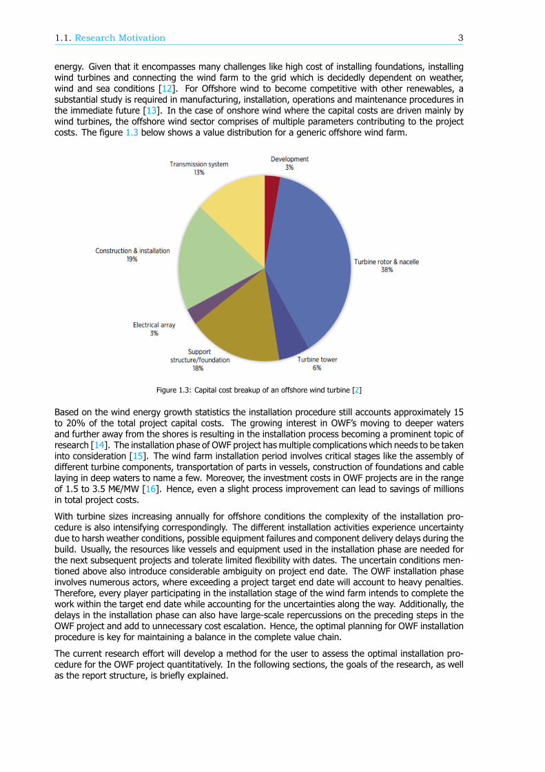
energy. Given that it encompasses many challenges like high cost of installing foundations, installingwind turbines and connecting the wind farm to the grid which is decidedly dependent on weather,wind and sea conditions [12]. For Offshore wind to become competitive with other renewables, asubstantial study is required in manufacturing, installation, operations and maintenance procedures inthe immediate future [13]. In the case of onshore wind where the capital costs are driven mainly bywind turbines, the offshore wind sector comprises of multiple parameters contributing to the projectcosts. The figure 1.3 below shows a value distribution for a generic offshore wind farm.
Figure 1.3: Capital cost breakup of an offshore wind turbine [2]
Based on the wind energy growth statistics the installation procedure still accounts approximately 15to 20% of the total project capital costs. The growing interest in OWF’s moving to deeper watersand further away from the shores is resulting in the installation process becoming a prominent topic ofresearch [14]. The installation phase of OWF project has multiple complications which needs to be takeninto consideration [15]. The wind farm installation period involves critical stages like the assembly ofdifferent turbine components, transportation of parts in vessels, construction of foundations and cablelaying in deep waters to name a few. Moreover, the investment costs in OWF projects are in the rangeof 1.5 to 3.5 M€/MW [16]. Hence, even a slight process improvement can lead to savings of millionsin total project costs.
With turbine sizes increasing annually for offshore conditions the complexity of the installation pro-cedure is also intensifying correspondingly. The different installation activities experience uncertaintydue to harsh weather conditions, possible equipment failures and component delivery delays during thebuild. Usually, the resources like vessels and equipment used in the installation phase are needed forthe next subsequent projects and tolerate limited flexibility with dates. The uncertain conditions men-tioned above also introduce considerable ambiguity on project end date. The OWF installation phaseinvolves numerous actors, where exceeding a project target end date will account to heavy penalties.Therefore, every player participating in the installation stage of the wind farm intends to complete thework within the target end date while accounting for the uncertainties along the way. Additionally, thedelays in the installation phase can also have large-scale repercussions on the preceding steps in theOWF project and add to unnecessary cost escalation. Hence, the optimal planning for OWF installationprocedure is key for maintaining a balance in the complete value chain.
The current research effort will develop a method for the user to assess the optimal installation pro-cedure for the OWF project quantitatively. In the following sections, the goals of the research, as wellas the report structure, is briefly explained.
4 1. Introduction
1.2. ObjectiveThe objective of the thesis study is outlined as:
“To have an approach supporting the decision maker to obtain minimized costs for OWF installationprocedure with a targeted completion date as a priority.”
Ultimately, the result of the project is to have a method that provides added flexibility to OWF instal-lation planning and estimates the most optimal solution in reasonable time frames. The points belowsummarize the different steps required to achieve the goal as mentioned above:
• Identify the key challenges to address in the ECN tool.
• Formulate the design problem and prepare installation tool for optimization analysis.
• Selection of suitable optimization model for the project.
• Provide flexibility to house a range of installation situations.
• Validate the necessary modules for the new approach.
• Run cases studies to reflect on the new approach towards solving installation scheduling problem.
1.3. Report OutlineChapter 1 through 2 provide introductory information with some background idea about the installa-tion planning problem. In Chapter 2 the different installation challenges are outlined, and the OWFinstallation problem is formulated. This chapter also includes existing literature work done in installa-tion scheduling problems. Chapter 3 introduces the automated planning approach to the reader anddescribes the methodology proposed for integrating the optimizer with the ECN Install. Chapter 4zooms into the optimizer and covers the topic of uncertainty quantification method implemented in theproject. Chapter 5 includes the various validations and verification done in the project. This chap-ter also contains the optimizer parameter tuning results. Later, Chapter 6 presents the case studiesdone in the project. Finally, Chapter 7 includes the conclusion of the thesis work and includes therecommendations for future research.

2Offshore Installation Scheduling
Problem
Installation scheduling is one of the critical steps demanding a high level of planning for the timelycompletion of a wind farm to go operational. The challenges with OWF logistics and installation processare associated with several factors. Distinguishing the issues relating to the installation procedure is ademanding activity, but on the other hand highly essential to identify the means to improve the existinginstallation process. The reader who is not familiar with OWF field is suggested to refer the Appendix Asection to get a basic understanding of the different resources and components used in the installationprocess. In the first section, the various challenges faced during the offshore wind farm installationprocedure are given. This is followed by a section dedicated to defining the optimization problem forOWF installation procedure. Finally, the chapter concludes with the proposed method to integrate theoptimization approach with ECN Install.
2.1. Offshore Wind Installation ChallengesOffshore wind farm installation is not a straightforward procedure and has many uncertainties to over-come. As explained in the introductory chapter the basis of optimizing installation process of OWF’sis linked to understanding the different challenges associated with it. Any installation phase is strictlybound by time, and total cost sustained during the building process. The various resources used duringthe installation period are expensive and have substantial contributions in the CAPEX of the project.The different vessels and labor chartering costs are the largest influencers for escalating the total ex-penses in a project. The subsections below recapitulates the key challenges encountered in the OWFinstallation industry depending on the activity under consideration.
2.1.1. FoundationsThe options for different foundation types are numerous with each one impacting the installation timeand cost differently. When comparing jackets and tripods with monopiles, the latter takes less timeto install as they are lighter, less complex structures and require fewer pile driving operations percomponent. Next, the water depth and soil type are critical parameters deciding the component outlayand installation period. The addition of scour protection increases the different vessel requirementsand add to the expenditure and duration of the project.
The installation vessels are the most important variable accounting for the maximum installation ex-penses. Thus, the selection of the right vessel for the installation activity is an essential task. Importantparameters like the vessel workability, crane specifications, speed and deck space determine not onlythe per foundation installation time but also impact on the total build time. Similarly, the choice ofthe port has significant repercussions on the project expenses and time duration. The harbor loca-
5
6 2. Offshore Installation Scheduling Problem
tion determines the fluidity of onshore logistics and the distance to farm. The offshore site distanceregulates vessel travel time and eventually effects the project CAPEX. When considering the weatherrestrictions for the foundation activities, they are less susceptible to wind conditions when comparingwith the turbine installation procedure. Nonetheless, weather delays can be expected due to severeweather conditions; again stressing the point about precise resource selection and planning.
2.1.2. Wind Turbines
The wind turbine installation activities over and above the reasons listed in section 2.1.1 are influencedby the total number of turbines to install, vessel selection, technicians experience and installation con-cept adopted for the project [3]. Unlike the foundations, the weather plays a central role while planningthe installation steps. This is due to the height of lift activities undertaken during turbine installation.These high lifts for crane mandate greater workability restrictions hence reducing the available weatherwindows for operation. Importantly, the turbine size and level of onshore assembly influence the totalinstallation time and eventually the cost sustained during the project. Finally, the sensitive dimensionsof wind turbine components augment the challenges in the wind turbine installation process.
2.1.3. Cables
The offshore wind farm consists of two different cable installation activities (Inter-array cables andexport cables). The bottlenecks in the installation are also dependent on the complexity of the project.To begin with, the cost and time for installing infield array cables are dependent on the number ofturbines, the layout of the farm, soil type, burial depth, scour protection requirements and so forth.While considering export cable installation the soil type, burial depth and location of the onshorestation are some of the critical parameters controlling the installation time. In both types of activities,the weight and length of the cables have a large impact on the total costs involved in the project.The dimensions of the cables influence the vessel selection and eventually the installation time ofthe activities. The cable laying installation ultimately is a trade-off between the vessel and the burialmethod implemented in the project.
2.1.4. Conclusion
There are other difficulties like the limited availability of purpose-built vessels for OWF installation mar-ket. Likewise, setting up the best possible loading sets on the vessels based on the weather windows isa big challenge. The possibility of component or equipment damage during the installation activity canseverely impact the project expenditures. Hence, it is important for a contractor or project developerto consider numerous uncertainties in a project and design the most optimal installation strategy tominimize the overall cost and duration. This study will look into some important factors affecting theOWF installation procedure and propose suitable solutions. It is an apt moment to define the scope ofthe thesis work to the reader. Although the optimization study in OWF installation scheduling is a largedomain, this thesis assumes the decision maker already knows the turbine, foundation type and the ca-ble specifications utilized in the wind farm. Similarly, the study does not look into the onshore logisticsand availability of resources during a project. It is assumed there are no delays in the onshore valuechain and all the required vessels or equipment are available during the installation planning stage.The scope of work is restricted towards optimizing the offshore installation scheduling problem with thecontinued availability of resources predefined by the user. Before we dive deeper into the optimizationproblem, it is essential to introduce the ECN Install tool for the reader to understand the key aspectsto address in the new approach. The optimization topic is introduced in section 2.3 subsequently afterthe reader gets an overview about ECN Install in section 2.2.
2.2. ECN Install 7
2.2. ECN InstallThis section takes forward the different wind farm components and resources and demonstrates themodeling approach followed in the software space. Chapter 1 gave a small introduction to the tool.This segment further covers the incentive for building ECN Install,with an outline of the user interfaceand the logic followed in the modeling.The Install package is based on MATLAB platform to supportthe back-end code and C program for the front end GUI (Graphical User Interface). The significance ofinstallation activity in the offshore wind industry is already outlined in section 1.1. Hence, a robust OWFinstallation planning tool can benefit multiple users like installation contractors, wind farm developers,institutions, etc. The tool aims to provide precise time and cost indications for various installationprocedures. It highlights the barriers during the installation activities and supports in eliminating projectrisks. ECN Install is designed to test various conceptual installation strategies for accelerating theknowledge transfer between different actors involved. It leads towards efficient resource managementto minimize the possible delays and overall costs for simulated schedules. The ECN Install simulationtool is in existence from early 2014, where over the years it has seen systematic improvements and gotassigned a particular version at every point. The final commercial tool is based on version 2.1 (startingnow referred to as ECN Install old). On the other hand, there are additions made in the back-endcode and an internal version is provided for this research study. The distinct differences between theversions will be highlighted when obligated in the report. In the version of the tool utilized for thisproject, a general simulation of the complete value chain of the OWF installation procedure can berepresented. ECN tool is a time driven simulation software which primarily facilitates in estimating atentative project completion time and the various costs involved during the installation procedure. Thetool provides excellent flexibility in the hands of the user to model the desired planning and export thecost and time outputs for any project. Due to the high reliance on the user-defined inputs, the outputsare profoundly dependent on the quality of input data. The following section breaks the ECN installinto blocks and explains the installation scheduling approach followed in the software.
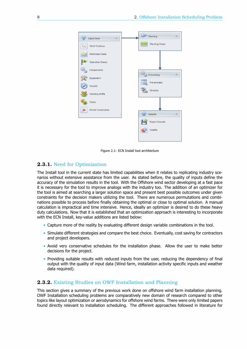
Tool Architecture
This section covers the modeling logic applied in the ECN Install tool. It should be clear to the readerfrom the figure 2.1 that the tool houses four key modules (Input Data, Planning, Processing, andResults). Starting with the input block which stockpiles all the parameters required for the followingblocks to run the simulation. This includes library of resources (Vessel, equipment, technicians, com-ponents), wind farm specifications (Wind turbine data, weather data, port) and other relevant costparameters required for the planning process. The Planning block shown in the figure below is wherethe user prepares the actual schedule for the installation activities to evaluate in the tool. The planningcomprises of a group of ‘Steps’ which further results in a collection of ‘Sequences’ (Refer figure B.1in Appendix B). The Processing module holds two blocks called the Pre-processor and the Simulatorrespectively. Pre-Processor tab aids to process the planning and inputs by the user without consideringthe various types of delays. The Simulator block as the name suggests simulates the planning basedon the weather data and outputs the new planning accounting for effects of delay. Lastly, the Results(Post-Processor) module contains the tabs to post-process the simulation solutions in a presentablemanner to facilitate decoding of the planning created initially. Each of the modules introduced aboveis explained more elaborately for more insight into the tool in appendix B. The reader is recommendedto refer to appendix B for better understanding about the working of ECN Install.
2.3. Optimization of Installation PlanningIn the field of technical analysis, optimization is the process of adjusting an existing procedure to makeit more efficient. These adjustments include selecting certain design variables and trying differentcombinations to move towards an optimal solution while eliminating the bad results along the way.Installation planning problems being very dynamic and difficulty in forecasting specific weather realiza-tions pose extra challenges in finding effective solutions. This section will justify the need for optimizerwith the ECN Install tool and the advantages which follow this decision.
8 2. Offshore Installation Scheduling Problem
Figure 2.1: ECN Install tool architecture
2.3.1. Need for OptimizationThe Install tool in the current state has limited capabilities when it relates to replicating industry sce-narios without extensive assistance from the user. As stated before, the quality of inputs define theaccuracy of the simulation results in the tool. With the Offshore wind sector developing at a fast paceit is necessary for the tool to improve analogs with the industry too. The addition of an optimizer forthe tool is aimed at searching a larger solution space and present best possible outcomes under givenconstraints for the decision makers utilizing the tool. There are numerous permutations and combi-nations possible to process before finally obtaining the optimal or close to optimal solution. A manualcalculation is impractical and time intensive. Hence, ideally an optimizer is desired to do these heavyduty calculations. Now that it is established that an optimization approach is interesting to incorporatewith the ECN Install, key-value additions are listed below:
• Capture more of the reality by evaluating different design variable combinations in the tool.
• Simulate different strategies and compare the best choice. Eventually, cost saving for contractorsand project developers.
• Avoid very conservative schedules for the installation phase. Allow the user to make betterdecisions for the project.
• Providing suitable results with reduced inputs from the user, reducing the dependency of finaloutput with the quality of input data (Wind farm, installation activity specific inputs and weatherdata required).
2.3.2. Existing Studies on OWF Installation and PlanningThis section gives a summary of the previous work done on offshore wind farm installation planning.OWF Installation scheduling problems are comparatively new domain of research compared to othertopics like layout optimization or aerodynamics for offshore wind farms. There were only limited papersfound directly relevant to installation scheduling. The different approaches followed in literature for
2.3. Optimization of Installation Planning 9
OWF installation procedure are highlighted here.
Scholz-Reiter et al.[17] introduce a mathematical model making use of mixed integer linear program-ming (MILP) with the goal of minimizing the total time for building the wind farm. Their model studiedthree different scenarios and examined the vessel requirements. The model calculated optimized load-ing sets, resource demands and optimal installation sequence for the different cases. A major drawbackof the model was its ability to run only for short time horizons. To overcome these limitations, Scholz-Reiter et al. [12] proposed a heuristic approach to solve a similar installation planning problem. Thenew approach was able to solve for longer time horizons with more complexity in installation activitiesfor varying weather states.
Next, Lutjen and Karimi [18] proposed a simulation approach for port inventory control system. Theyalso followed a heuristic approach based on the one developed in [12] to simulate the installationplanning process. They finally present the two-level approach of scheduling and inventory management(material restock) for offshore wind farms.
Ait-Alla et al. [19] introduce a model to deal with aggregated installation planning problem. The paperconsiders operational constraints like weather and vessel availability. Weather windows are split intocategories from good to bad conditions in the problem. The model generates an estimated mediumplanning horizon schedule which minimizes the total costs of the given project. The model takes intoconsideration the costs and weather restrictions per vessel type selected for installation.
Y.T. Muhabie et al. [20] shows a new approach to tackle the offshore wind farm installation problem.The help of Discrete Event Simulation (DES) is applied to model weather, vessel characteristics andturbine assembly scenarios. The simulation is carried out with both historical weather realizationsand probabilistic approach. In the probabilistic approach, various distributions are prepared in thesimulation depending on the weather window required and the resource weather restrictions. The DESmethod considers only points in time (events) and instances in between are not of interest. It is apopular approach used in transportation management, flow management and management of failures.The findings provide a new framework to address risks and uncertainties in OWF installations.
The C .A. Irawan et al. [21] work addresses the optimization work in the offshore wind farm installationplanning. A bi-objective optimization for minimizing the costs and completion period of the installationscheduling problem is presented. The authors suggest two different approaches to solve the multi-objective problem. One using compromise programming with the exact method and the other withmetaheuristic techniques. The paper makes an interesting conclusion on the different approaches,where the exact method attains optimality for all cases. However, the increase in the size of theproblem resulted in an exponential growth in computation time for the exact method when comparedto metaheuristic approach. The metaheuristic approach ran much faster and produced well overall.
Therefore, based on the learning from the existing literature work the next section will focus on selectingan appropriate optimizer and integrating it with ECN Install tool.
2.3.3. Optimization ChoicesEvery problem has certain select optimization compatibility based on the problem setup. The optimalsolution for a problem can be found either by exhaustive search or using an optimal finding algorithmfor any planning problem. A big drawback of the exhaustive search is the time taken to obtain anoptimal solution. On the other hand, algorithms dedicated to finding local or global optimum solutionsare much faster at converging to the desired solution.
When the optimization choice for ECN Install is under consideration, it is important to evaluate theproblem setup and the possible design space for the optimizer. Any optimizer linked to the Install toolwill need to input a combination of design variables and allow the ECN tool to work as a black boxto evaluate the combination and deliver the results. These results would be later passed through theoptimizer to select the most optimal solution. Thus, it is essential to pick a derivative-free optimizationalgorithm to satisfy the needs as mentioned earlier. This project includes a large design space for theoptimizer to look for an optimal solution and hence to avoid any sub-optimal solutions a global searchoptimizer is preferred.
10 2. Offshore Installation Scheduling Problem
Due to the high complexity of optimization problems under uncertainty, time and again traditional ap-proaches which assure optimal solutions tend to be reasonable only for small problem sizes. Theyrequire a great deal of computational power to function for large instances. Stochastic optimizationis the general class of techniques which use some degree of randomness to find good (or sometimesoptimal) solutions to hard problems [22]. Metaheuristics are the most general of these kinds of al-gorithms and are applied to an extensive range of problems [23]. There are different metaheuristicapproaches, but this report only considers search algorithms. It is mainly due to their popularity andflexibility to adapt to different problems easily.
By listing the above requirements, a global search and gradient free algorithm are desired for thisproject. It is preferred to develop a custom-made algorithm for the design problem, nonetheless is avery time-consuming and complex proposition. Considering the effort required for development andtime limitations for the project the MATLAB optimization toolbox is chosen for carrying out the studywith ECN Install tool. MATLAB platform provides three global search algorithms in the toolkit. TheGenetic algorithm (GA), Particle swarm optimization (PSO) and Simulated annealing (SA) [4]. Theproblem representation differs for every algorithm mentioned above and testing each one is not apragmatic approach. It is later found that the problem representation of GA and PSO methods aremore comparable [24][25]. The GA is selected for the project as it is a very popular algorithm withlarge literature base for assistance. The GA toolbox is easy to adapt to different design challenges,and the problem representation could be altered for PSO method in future with little effort if necessary.Moreover, it is the only algorithm providing a ready option for evaluating integer constrained designvariables. The GA is a population-based approach which means it would evaluate multiple parametercombinations in one iteration. This feature would be beneficial while dealing with large installationproblems with a high count of design variable evaluations. Lastly, the toolbox also provides the multi-objective capabilities which could be used in the future. Ultimately, it should be clarified that the specificoptimizer selected for the project is one of the ways to solve the installation problem and not the onlychoice suggested by the author.
2.4. Optimizer Addition to ECN InstallThe introduction of optimizer calls for certain modifications to the existing architecture of ECN Install.The block diagram below shows the methodology to integrate the Genetic algorithm optimizer with ECNInstall together. The introduction of an optimizer with the ECN Install tool requires the development ofsupporting blocks for the optimization approach to function appropriately. Referring to the figure 2.2,starting with the first block in black which has the primary purpose of collecting all the wind farm andproject data for any installation planning in study. The existing blocks from the old architecture of ECNInstall are highlighted in grey shades. These comprise of the weather simulator introduced in B.0.5 andthe ECN Install tool itself. The two primary additions are the automated planning (in chapter 3) andoptimizer blocks (covered in chapter 4). The initial planning block as the name suggests works on thesame principals of the automated planning block, although its functionality is restricted to initializing theproject before proceeding into optimization phase. In this project weather is the only uncertain variableconsidered throughout the study. Based on the overview given about the new weather simulator, theuncertainty consideration for the results from ECN Install is carried out in the UC block (in chapter 4).Reviewing the objective defined in section 1.2, there is a requirement to evaluate the project end datein this study which is achieved in CV block (in chapter 4).The optimization analysis with ECN Installis a repetitive process where different design variable combinations are tried till the optimal result isachieved. Once the best combination is obtained, this is represented by the optimal solution block ingreen. To indicate the repetitive process of the optimizer the loop is highlighted with a dashed blockand red arrows for the reader.
The block diagram above represents the problem approach adopted for this research work. The fol-lowing chapters will elaborate the various blocks in detail and provide more insight to the reader aboutthe integration process with ECN Install.

2.4. Optimizer Addition to ECN Install 11
Figure 2.2: New project architecture

3Automated Planning
This chapter covers the methodology applied for generating the Automated Planning (AP) based onthe initial inputs for the project. The following sections explain the primary requirement of this blockin the project. This is followed by a summary of the limitations and benefits of using this approachand the various assumptions made in the modeling process. Next, a section is dedicated for a deeperunderstanding into the course of translating the inputs from the user into installation planning for ECNInstall tool. Finally, the last part explains how the automated planning is integrated into the optimizerloop as shown in figure 2.2 (chapter 2).
3.1. Automated Planning RequirementThe current commercial version of ECN Install requests the user to create the complete time andresource planning for any project. This approach was sufficient as all the resources remained fixed andthe ECN Install accounted for uncertainty due to weather and translated the delays in the form of costsand time values. The addition of an optimizer with ECN Install software entails certain changes to theold architecture as introduced in section 2.4. Unlike the old approach where fixed user inputs are usedfor simulations the new method iterates various combination of different resources to find the optimalsolution. Hence, there is a need to automate the planning processes to allow the optimizer to make suchchanges dynamically during the GA optimization. In the new methodology, the user provides certainfixed parameters for the project that do not alter during the complete installation schedule evaluation.The rest of the process is automated based on the particular choice of resource in the planning (doneby the optimizer). While the requirement of AP block is unavoidable it brings certain advantages andsome limitations to take into consideration. The new approach reduces the project planning time tofew minutes compared to hour or more depending on the complexity of schedule. Additionally, the useris no longer required to calculate the precise number of repetitions of activities which was previouslymandatory. On the contrary, AP block approach operates with pre-defined templates for differentinstallation procedures. Hence, limiting the flexibility to make changes in the sequence of installationactivities. The different inputs and logic behind the planning process will be explained in the sectionsto follow.
3.2. Automated Planning BlocksAutomated planning in the software platform is created using a standardized approach for differentinstallation components. The specific blocks vary based on the installation activity, but the logic behindthe building process remains the same. The block diagram below shows the basic approach used in theplanning process. The block diagram explains the process during the initialization process where theuser inputs are stored first. Installation Type block is where the scope of the project is decided (refertable 3.1). The Selection and Build block constructs the planning based on the inputs from the previous
13

14 3. Automated Planning
blocks. This block retrieves the required information from the different libraries explained in the nextsection. The planning and the inputs are stored in the mandatory Database format to simulate theplanning in ECN Install software. The installation sequence module shows a typical sequence createdin the automated planning block. The specific steps change based on the installation activity, but thelogic behind the formulation of the planning is very similar. Three types of blocks namely Loading,Traveling and Installation are used as the backbone structure for any installation sequence planning.The section 3.4 of this chapter explains the use of these three blocks in different installation scenarios.
Installation Type
Selection & Build
Installation Steps
Travel to New Turbine
Location
Installation Sequence
Input
ECN Install DATABASE Template
Equipment Library
Vessel Type Library
Harbor Library
Travel
Travel
Loading / Mobilization
Figure 3.1: Automated planning flow diagram
3.3. AP Block InputsThe inputs from the user need to be passed in a predefined format that is accepted by ECN Install.As the automated planning is finally aimed to feed the schedule into ECN simulator, the same formatis required to be followed for the automated planning to work with ECN Install. The data handlingprocess in the ECN Install is explained in appendix C for interested readers.
The following section explains the various inputs given by the user to generate the automated planningfor each installation process.First, the necessary resources involved in the OWF installation schedulingproblem are identified. The engineering choice of resources like the vessel, equipment, and port isfound to be most important to look into [26] in the current work. Once this aspect is established theresource classification is necessary for the software implementation. Specific resource Libraries arecreated inside AP module to access common information for every planning. The following subsectionswill look into the classifications and cover the reasons behind creating the classifications inside eachlibrary. The library serves as a common point for the AP block to select a suitable resource for theplanning. The next subsections explain the different libraries in more detail.
Building on the introduction from section 3.1, the automated planning block still requires specified inputsfrom the user to create the necessary planning. Table 3.1 summarizes the general inputs needed forsimulating a typical project in ECN Install running with automated planning approach. The specificinputs for installation activities like foundations and wind turbines are covered in section 3.4 with moredetails.
3.3. AP Block Inputs 15
Input Parameter Remarks
Project complexity
1.Only foundation installation
2.Foundations + wind turbines installation
3.Foundations + wind turbines+ infield cable installation
Note: Scour protection option available for all 3 options
Wind farm location GPS coordinates of the OWF location (In degrees)
Wind farm
1.Total number of wind turbines
2.Number of turbines, wind turbine power curve(optional) and hub height.
3.Number of turbines, wind turbine power curve(optional) and hub height.
Weather data Wind and wave height data for wind farm location and ports (optional)
Fixed costs (optional) Miscellaneous fixed costs and project management costs
Table 3.1: Project inputs
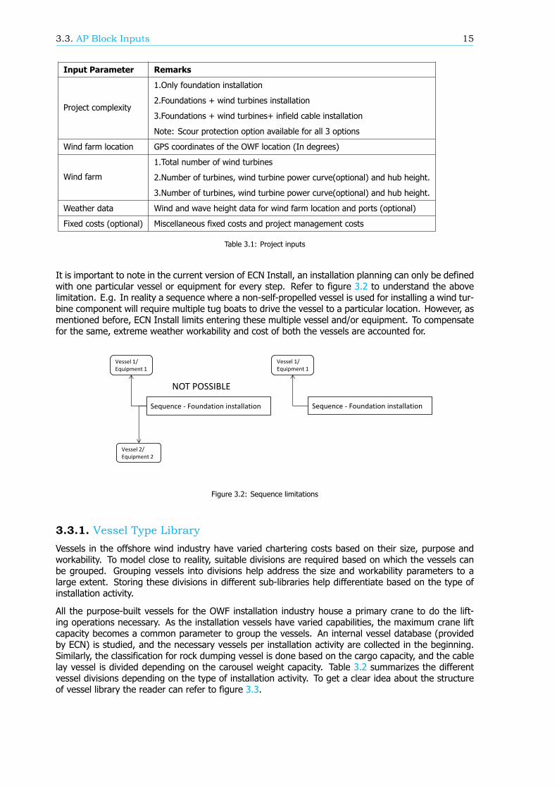
It is important to note in the current version of ECN Install, an installation planning can only be definedwith one particular vessel or equipment for every step. Refer to figure 3.2 to understand the abovelimitation. E.g. In reality a sequence where a non-self-propelled vessel is used for installing a wind tur-bine component will require multiple tug boats to drive the vessel to a particular location. However, asmentioned before, ECN Install limits entering these multiple vessel and/or equipment. To compensatefor the same, extreme weather workability and cost of both the vessels are accounted for.
Figure 3.2: Sequence limitations
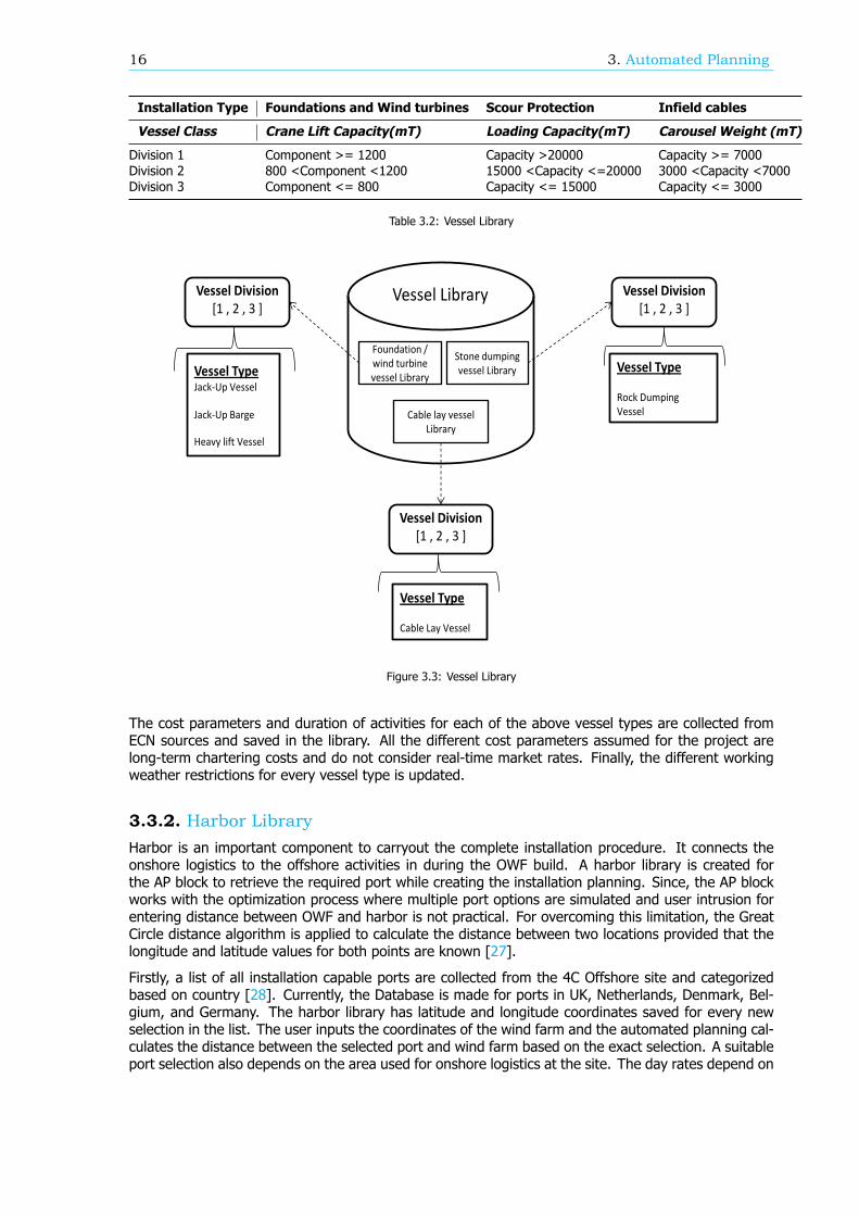
3.3.1. Vessel Type LibraryVessels in the offshore wind industry have varied chartering costs based on their size, purpose andworkability. To model close to reality, suitable divisions are required based on which the vessels canbe grouped. Grouping vessels into divisions help address the size and workability parameters to alarge extent. Storing these divisions in different sub-libraries help differentiate based on the type ofinstallation activity.
All the purpose-built vessels for the OWF installation industry house a primary crane to do the lift-ing operations necessary. As the installation vessels have varied capabilities, the maximum crane liftcapacity becomes a common parameter to group the vessels. An internal vessel database (providedby ECN) is studied, and the necessary vessels per installation activity are collected in the beginning.Similarly, the classification for rock dumping vessel is done based on the cargo capacity, and the cablelay vessel is divided depending on the carousel weight capacity. Table 3.2 summarizes the differentvessel divisions depending on the type of installation activity. To get a clear idea about the structureof vessel library the reader can refer to figure 3.3.
16 3. Automated Planning
Installation Type Foundations and Wind turbines Scour Protection Infield cables
Vessel Class Crane Lift Capacity(mT) Loading Capacity(mT) Carousel Weight (mT)
Division 1 Component >= 1200 Capacity >20000 Capacity >= 7000Division 2 800 <Component <1200 15000 <Capacity <=20000 3000 <Capacity <7000Division 3 Component <= 800 Capacity <= 15000 Capacity <= 3000
Table 3.2: Vessel Library
Figure 3.3: Vessel Library
The cost parameters and duration of activities for each of the above vessel types are collected fromECN sources and saved in the library. All the different cost parameters assumed for the project arelong-term chartering costs and do not consider real-time market rates. Finally, the different workingweather restrictions for every vessel type is updated.
3.3.2. Harbor LibraryHarbor is an important component to carryout the complete installation procedure. It connects theonshore logistics to the offshore activities in during the OWF build. A harbor library is created forthe AP block to retrieve the required port while creating the installation planning. Since, the AP blockworks with the optimization process where multiple port options are simulated and user intrusion forentering distance between OWF and harbor is not practical. For overcoming this limitation, the GreatCircle distance algorithm is applied to calculate the distance between two locations provided that thelongitude and latitude values for both points are known [27].
Firstly, a list of all installation capable ports are collected from the 4C Offshore site and categorizedbased on country [28]. Currently, the Database is made for ports in UK, Netherlands, Denmark, Bel-gium, and Germany. The harbor library has latitude and longitude coordinates saved for every newselection in the list. The user inputs the coordinates of the wind farm and the automated planning cal-culates the distance between the selected port and wind farm based on the exact selection. A suitableport selection also depends on the area used for onshore logistics at the site. The day rates depend on
3.4. AP block implementation 17
the actual area utilized and as this falls under the onshore resource optimization domain it is excludedfrom current work. For simplicity a fixed day rate value is assumed for all the harbor locations in library.
3.3.3. Equipment LibraryThe Equipment Library is created based on the type of installation type selected. Currently, the equip-ment used is relatively standardized with limited choices. It is created for the AP block to choose therelevant equipment based on the installation activity and also planning for future situations if morenumber of options would be available to install the same resource.
3.3.4. Default Database TemplateAs explained in section 3.3, the MATLAB code of ECN Install accepts the user inputs and planninginformation in a specified manner. This requirement is adhered to and all the inputs and automatedplanning is reproduced in the same required format for the tool. There is a Default template file usedas a starting point for storing the data in the desired format. The template block can be seen in figure3.1 after the Selection & build module.
3.4. AP block implementationThis sections initially lists the different assumptions taken into consideration while modeling the AP blockapproach. This is followed by the description about the procedure followed in implementing automatedplanning for different installation procedures. As stated before, the automated planning prepares aninstallation planning based on a user selected installation strategy. The specific assumptions consideredfor the AP block modeling approach are listed below:
• The Wind turbine type and farm size for installation planning are fixed. Thus, the decision makeris required to know the number of turbines, turbine class (MW rating), and power curve(optional)before running the AP procedure.
• The installation activity templates are pre-defined. This saves considerable amount of time foruser during input stage but on the contrary limits the flexibility in installation schedules.
• Number of technicians per type of activity are fixed. The required number of technicians aredecided based on old wind farm projects. The user is still given the option to overwrite thedefault values with the ones required for the specific simulation.
• All the planning is created following a 24/7 working period (mostly followed in offshore windindustry).
• Component cost1 is not considered in the automated planning process. I.e. only installation costis the main parameter of study from the CAPEX2.This data is set to zero in the AP block.
• The different vessels and equipment are classified per type. The specifications of the resources(Vessels/equipment) under the same category are alike.
• The duration of installation activities (Step level) are fixed per type of resource. There is provisionto change the values in MATLAB code if the user desires.
• Multiple vessel concepts are not modelled within particular sequence of activities.(explained insection 3.3)
• Fixed activity duration is assumed in automated planning block. The activity duration is fixed todefault value which does not change during the complete simulation.
Section 3.3 gives an overview of the automated planning approach modelled in this study. The followingparts describe the method followed for different installation activities.
1Cost of manufacturing foundations, wind turbine components and transmission cables etc.2Capital expenditure (CAPEX) are the expenses incurred in building the complete value chain of the OWF. It accounts for varioustypes of expenditures as shown in figure 1.3.
18 3. Automated Planning
Scour Protection
Scour is a type of erosion of soil around the structure in the seabed. This is especially significant inlocations with tidal currents around the structure [29]. In such cases, it becomes beneficial to preparea rock bed around the structure to avoid the above scenario. Scour protection is applied to foundationswhich are secured to the seabed. The rock dumping is performed in phases where first the small rocksare precisely dropped around the substructure location. The next step of the rock dumping is doneafter the foundations are installed where large stones are placed to secure the scour protection fromeroding away over time [3].
Software Implementation
The installation procedure for scour protection case is included in the automated planning process. Itis provided as an option to the user to select for the project. The scour protection follows the samebuilding processes as seen in figure 3.1. During the installation step if the user does not input theamount of rock dumping per foundation location a default value of 2300 tons is fixed in the simulation[30]. Using the pre-defined template for scour protection installation the AP block builds the loadingand traveling process for completing the sequence planning.
Wind turbine Foundations
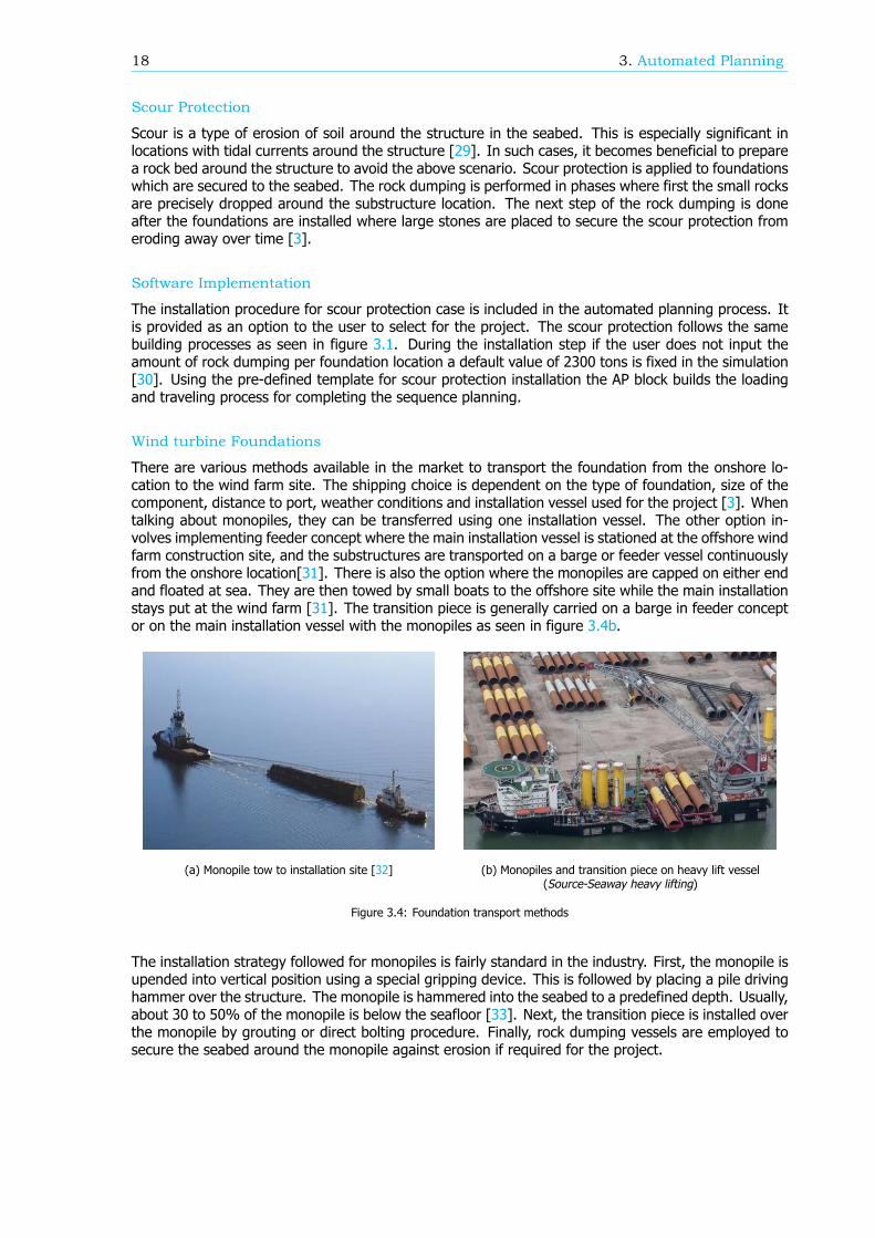
There are various methods available in the market to transport the foundation from the onshore lo-cation to the wind farm site. The shipping choice is dependent on the type of foundation, size of thecomponent, distance to port, weather conditions and installation vessel used for the project [3]. Whentalking about monopiles, they can be transferred using one installation vessel. The other option in-volves implementing feeder concept where the main installation vessel is stationed at the offshore windfarm construction site, and the substructures are transported on a barge or feeder vessel continuouslyfrom the onshore location[31]. There is also the option where the monopiles are capped on either endand floated at sea. They are then towed by small boats to the offshore site while the main installationstays put at the wind farm [31]. The transition piece is generally carried on a barge in feeder conceptor on the main installation vessel with the monopiles as seen in figure 3.4b.
(a) Monopile tow to installation site [32] (b) Monopiles and transition piece on heavy lift vessel(Source-Seaway heavy lifting)
Figure 3.4: Foundation transport methods
The installation strategy followed for monopiles is fairly standard in the industry. First, the monopile isupended into vertical position using a special gripping device. This is followed by placing a pile drivinghammer over the structure. The monopile is hammered into the seabed to a predefined depth. Usually,about 30 to 50% of the monopile is below the seafloor [33]. Next, the transition piece is installed overthe monopile by grouting or direct bolting procedure. Finally, rock dumping vessels are employed tosecure the seabed around the monopile against erosion if required for the project.

3.4. AP block implementation 19
Software Implementation
The automated planning approach models the foundation transport with a single vessel concept. Thesteps are split into four categories. The Loading step, Traveling step, installation step and finally theTraveling step again to conclude the iteration. The loading step is where the foundation componentsare stacked onto the vessel to be sailed to wind farm location. Next, the traveling step is executedwhere the vessel sails from the harbor to the wind farm site. The installation step contains the specificinstallation operations like the one mentioned above. Once the installation work is complete the vesselsails inside the wind farm to a new location, repeating the installation activity until all components arein place. Finally, the empty vessel travels back to the harbor which is represented by the traveling stepto repeat the above process up until the necessary installations are completed.
Infield Cabling
The array cable installation process is essential in connecting the different wind turbines in the farmto the grid. A few popular offshore cable installation methods are explained in this section. After thecables are laid on the seabed they also need to be buried a few meters below the ocean floor for safety[34]. There are two popular methods relevant for the wind industry.
Cable lay and bury: In this approach, the specific section of the sea floor is unearthed using a purpose-built dredging vessel. Once the process is completed, the cable is laid inside the furrow using a cablelaying vessel. The furrow is later covered using a dredge. This method is utilized for both infield andexport cables laying procedure.
Simultaneous lay and bury: The cable laying vessel has a large turntable with the cable to be installed.These vessels are equipped with a plow or supported by a different vessel to create a trench forlaying the cable in the seabed. High-pressure water jets are popularly used to diffuse the seabed andsimultaneously bury the cables. The other method in the same class employs a Remotely OperatedUnderwater Vehicle (ROV) in place of a plow. This method is popularly used in infield array cableinstallations where the ROV buries the cables under the seabed [30].
At the outset, the vessel positions itself close to the foundation for starting the cable lay process. Everyfoundation installed offshore is preserved with a messenger wire close to the cable entry point on thefoundation. This messenger wire is recovered and connected with the actual array cable on board thevessel. Next, the pull-in operation is carried out, and the array cable is secured to the foundation.The vessel starts the laying process on the seabed until it reaches the next foundation site. The samepull-in operation is done at the new foundation site, and the iterative approach continues until thecompletion of cable laying procedure [35]. Once the cable is laid, a different vessel is deployed tobury the cable for safety reasons. A working class ROV is used to complete the cable installationactivity. This project considers only inter/infield cable installation in the OWF planning and excludesthe OHVS (Offshore High Voltage Station) and export cable works. It is observed that Transmissionsystem operators (TSO) in countries like Netherlands, Germany, and Denmark are given responsibilityto build offshore grid network to facilitate the linking of multiple wind farms in the North Sea [36].Hence, this section only covers the installation strategy applied in the wind farm cable network.
Software Implementation
The array cable installation is split into two sequences of activities. One responsible for the cable layprocess and the other for the cable bury phase. The required length of the infield cables is loaded ontothe cable lay carousel. The vessel thereafter travels to the wind farm location to begin the installationactivity. The simultaneous lay and bury approach explained in the above subsection is modeled forinstalling the cables. Once the installation is complete, the vessel returns to port and prepares for newload out, if necessary. To make the process automated for the user the cable weight per meter (40kg/m) [37] and the distance between the turbines (7 times rotor Diameter) are preset [38]. The useris given the option to change these parameters depending on the project specifications. The aboveassumptions allow the AP block to generate the array cable sequence with limited inputs from the user.
20 3. Automated Planning
Wind turbines
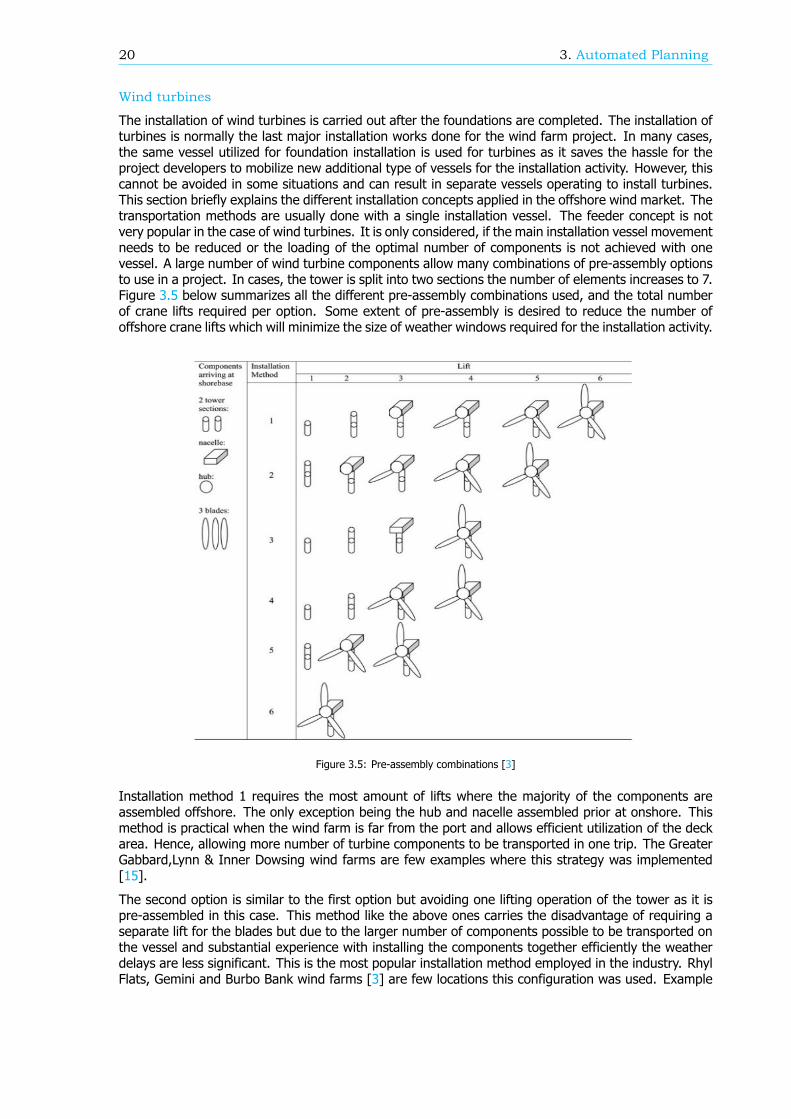
The installation of wind turbines is carried out after the foundations are completed. The installation ofturbines is normally the last major installation works done for the wind farm project. In many cases,the same vessel utilized for foundation installation is used for turbines as it saves the hassle for theproject developers to mobilize new additional type of vessels for the installation activity. However, thiscannot be avoided in some situations and can result in separate vessels operating to install turbines.This section briefly explains the different installation concepts applied in the offshore wind market. Thetransportation methods are usually done with a single installation vessel. The feeder concept is notvery popular in the case of wind turbines. It is only considered, if the main installation vessel movementneeds to be reduced or the loading of the optimal number of components is not achieved with onevessel. A large number of wind turbine components allow many combinations of pre-assembly optionsto use in a project. In cases, the tower is split into two sections the number of elements increases to 7.Figure 3.5 below summarizes all the different pre-assembly combinations used, and the total numberof crane lifts required per option. Some extent of pre-assembly is desired to reduce the number ofoffshore crane lifts which will minimize the size of weather windows required for the installation activity.
Figure 3.5: Pre-assembly combinations [3]
Installation method 1 requires the most amount of lifts where the majority of the components areassembled offshore. The only exception being the hub and nacelle assembled prior at onshore. Thismethod is practical when the wind farm is far from the port and allows efficient utilization of the deckarea. Hence, allowing more number of turbine components to be transported in one trip. The GreaterGabbard,Lynn & Inner Dowsing wind farms are few examples where this strategy was implemented[15].
The second option is similar to the first option but avoiding one lifting operation of the tower as it ispre-assembled in this case. This method like the above ones carries the disadvantage of requiring aseparate lift for the blades but due to the larger number of components possible to be transported onthe vessel and substantial experience with installing the components together efficiently the weatherdelays are less significant. This is the most popular installation method employed in the industry. RhylFlats, Gemini and Burbo Bank wind farms [3] are few locations this configuration was used. Example
3.5. Interdependency between Sequences 21
of the installation steps are shown in figure 3.6a , 3.6b , 3.6c.
In the third method, the rotor and three blades are assembled onshore, and the tower is transported in2 parts with the nacelle separately. Initially, the two sections of the tower are installed. It is followedby the installation of nacelle section. This method eliminates the lifts for the blades and requires justone lift to install the entire rotor(refer figure 3.6e). As a trade-off, the number of components carriedon the vessel is reduced compared to the above options. The Horns Rev 2 and Nysted wind farms usedthis configuration [15].
The fourth and fifth option employ what is called the “bunny ear” configuration. In this method, therotor and two blades are assembled in a bunny ear setup. Finally, one blade is installed separately atthe offshore site. The only minor difference lies in the pre-assembly of the tower in the fifth methodwhich is missing in option four. This configuration also demands different cranes to install the bunnyear configuration and is not a popular choice in the installation market shown in figure 3.6f. This optionwas implemented in North Hoyle, Barrow and Scroby Sands wind farms to name a few [15].
The final concept suggests the complete assembly of the turbine onshore. The assembled turbine iscarried on a barge or installation vessel and installed on the foundation. This method requires a heavylift crane vessel to carry out the installation activity. This option is not actively used in the industry yetdue to the complexities of lifting a delicate turbine assembly in offshore conditions. This method wastested in the Hywind pilot park offshore project seen in figure 3.6d [39].
Software Implementation
Wind turbine installation modeling can be done in many combinations. However, to simplify the process,the three widely used methods are identified and translated into planning templates. The option 2,3and 5 from figure 3.5 are the selected choices to implement in the software [3]. The wind turbineinstallation follows the same sequence as shown in figure 3.1. At first installation vessels usuallyundertake a mobilization process where they are fitted with a purpose built equipment to aid duringthe building phase. Based on the vessel type and pre-assembly configuration the AP block decidesthe loadout count for the components. Next, the travel and the installation steps are executed for thedesired planning. Wind turbine installation activities demand high elevation crane lift hence the toolextrapolates the wind speeds at those heights to improve modeling accuracy.
3.5. Interdependency between SequencesIn the current version of ECN Install while simulating multiple sequences of installation activities, forexample, foundation work, array cable installation or wind turbine installation; the user can define aparticular start date for every sequence exclusively. Unfortunately, while simulating a multi-sequencecase in optimization analysis, the objective function demands to minimize the total project cost whichis not possible until the sequences are linked together. To overcome the above limitation a basicsequence-sequence interdependency is implemented. Figure 3.7 below gives a better understanding.
In essence, the end of a step inside the first sequence provides the start date for the next sequence.The exact point of the link in the first sequence is for the decision maker to choose. The user alsocan decide a fixed number of days delay after the completion of the first sequence. To differentiatebetween the different interdependency, every sequence is represented with a unique number basedon its installation activity. For instance, the foundation installation activity is given a number 1, andthe wind turbine installation sequence is specified a number 2. The user is free to fix the exact gapbetween both the sequences depending on the reference numbers. The unique reference approach isespecially advantageous when two different vessels are installing the same component (foundationsor turbines). In such cases, the sequences will have the same number, and the automated planningprocedure spits the installation activity between the sequences and assigns the same start date to bothsequences. This is illustrated in figure 3.8.
As an illustration, two vessels are selected by the optimizer as a combination to install 100 foundationsin total. The automated planning will generate two unique sequences for each vessel for installing thefoundations. In cases the sequence numbers are the same, each vessel is assigned 50 foundations

22 3. Automated Planning
(a) Tower section installation (source-Offshoretechnology)
(b) Single blade installation(source-EDF Energy)
(c) Nacelle installation (source-Jack-up barge) (d) Complete turbine lift (source-Hywind)
(e) Full rotor lift (Source-Brave Tern) (f) Bunny ear assemblyinstallation (Source- Seajacks)
Figure 3.6: Pre-assembly Concepts applied in the industry

3.6. Automated Planning Integration with Optimizer 23
Figure 3.7: Interdependency between different sequences
Figure 3.8: Interdependency with multiple vessels
to install separately and are allocated with the same start date for both sequences. In the currentresearch, a simple sequence level interdependency is presented which works efficiently with the op-timization approach to account for the total costs and time for the simulated schedules. If complexinterdependency between different step level activities are included in later ECN Install releases, theautomated planning block will require major modification to adapt to real-time changes in the order ofactivities.
3.6. Automated Planning Integration with Optimizer
The primary automated block is split into two sub-blocks. One of these blocks is dedicated to initializingthe planning file called as the IP block (refer to figure 3.9). At this point, the fixed parameters for theinstallation scheduling case are saved. The fixed database template is subsequently passed insidethe optimization loop (marked in red). There is a separate planning block named as AP to handlethe changes in the optimization process. AP block automatically creates the planning based on thechanges in design variables. The different design variables for the project and the related optimizationparameters are discussed in next chapter in more detail. Zooming into the AP block shows the planningmodule containing two important sub-blocks. The Design variable processing block is developed totranslate the optimizer choices into solution space variables of ECN Install tool. The following blockcreates the new planning based on the optimizer variable changes. Finally, before passing the datainto ECN install a feasibility check of design variables is done to filter infeasible choices. For example,a jack-up barge has a 850 tonne crane lift capacity while a heavy lift vessel in the same division hasa 1000 tonne crane lift capacity. Assuming the component to install is 900 tonnes the jack-up bargeis not possible to use for installation and is filtered out before running in ECN Install. This block isintroduced to avoid running additional runs in ECN install and save overall optimization analysis time.Now that the reader has got a grasp on the ancillary blocks for study, the next chapter will dive intothe optimizer block.

24 3. Automated Planning
Weather
Simulator Initial planning (IP)
User Input
(OWF Installation data)
Constraint Evaluation (CV)
Optimal
solution
ECN Install
Uncertainty Consideration (UC)
Automated
planning (AP)
Optimizer (O)
New planning
Design variable
processing
Solution feasibility
AP Block
Figure 3.9: AP block in Project architecture
3.7. AP Block VerificationPrevious sections of the chapter describe the need and the procedure behind working of the AP blockin this study. To ensure proper functioning of the AP block for building correct planning, a specific testcase is prepared to verify the automated planning implementation in this research. Verification is thetask of establishing if the model execution is done appropriately. The verification is done by comparingduration and cost of an installation sequence that is build with AP block and later simulated in ECNInstall old (v2.1).
Without this step, there is no guarantee about the quality of results obtained from the optimizationprocedure. A part of an existing wind farm installation project is recreated in ECN Install old for the ver-ification process. Since ECN Install does not allow interdependency between different sequences, theverification process is carried out for a single installation sequence only. The table below summarizesthe AP block inputs:
Parameter Remarks
Weather data 5 years of wind [m/s] and significant wave height [m]Foundation type Monopile & Transition pieceNumber of foundations 90Vessel type Jack-up vesselStart date June, 2015Harbor Eemshaven,NL
Table 3.3: Verification sequence inputs
A two step process is followed for the verification procedure.The steps are listed below;
1. Comparison of ECN Install v2.1 and v2.2
2. Comparison of ECN Install v2.2 and AP block method
As explained, a similar planning is created in ECN Install old (v2.1) with necessary inputs. Figure3.10 shows the planning created in ECN Install old. It is ensured that the cost parameters of thevessel, equipment, and port are the same for both cases. Even though the AP blocks work inside the
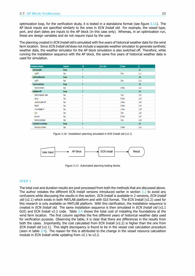
3.7. AP Block Verification 25
optimization loop, for the verification study, it is tested in a standalone format (see figure 3.11). TheAP block inputs are specified similarly to the ones in ECN Install old. For example, the vessel type,port, and start dates are inputs to the AP block (in this case only). Whereas, in an optimization run,these are design variables and do not require input by the user.
The planning created in ECN Install old is simulated with five years of historical weather data for the windfarm location. Since ECN Install old does not include a separate weather simulator to generate syntheticweather data, the weather simulator for the AP block simulation is also switched off. Therefore, whilerunning the installation sequence with the AP block, the same five years of historical weather data isused for simulation.
Figure 3.10: Installation planning simulated in ECN Install old (v2.1)
Figure 3.11: Automated planning testing blocks
STEP 1
The total cost and duration results are post-processed from both the methods that are discussed above.The author restates the different ECN install versions introduced earlier in section 2.2 to avoid anyconfusions while discussing the results in this section. ECN Install is available in 2 versions, ECN Installold (v2.1) which exists in both MATLAB platform and with GUI format. The ECN Install (v2.2) used forthis research is only available on MATLAB platform. With this clarification, the installation sequence iscreated in ECN Install old. The same installation sequence is then simulated in ECN Install old (v2.1GUI) and ECN Install v2.2 code. Table 3.4 shows the total cost of installing the foundations at thewind farm location. The first column signifies the five different years of historical weather data usedfor verification purpose. Observing the table, it is clear that there are differences in the results fromboth the cases. Importantly, the cost calculated from ECN Install (v2.2) is higher than the one fromECN Install old (v2.1). This slight discrepancy is found to be in the vessel cost calculation procedure(seen in table 3.4). The reason for this is attributed to the change in the vessel resource calculationmodule in ECN Install while updating from v2.1 to v2.2.

26 3. Automated Planning
Simulationyear
ECN Install total cost(K€)[v2.1 GUI]
ECN Install total cost(K€)[MATLAB v2.2]
Differencein results (K€)
1 30,884 30,934 502 30,809 30,909 1003 30,670 30,770 1004 31,425 31,425 05 29,461 29,511 50
Simulationyear
Vessel total cost(K€)[v2.1]
Vessel total cost(K€)(v2.2)
Differencein results(K€)
1 25,050 25,100 502 25,000 25,100 1003 25,000 25,100 1004 25,600 25,600 05 23,900 23,950 50
Table 3.4: ECN Install old (v2.1) vs ECN Install (2.2) results
STEP 2
As stated before, the second step followed in the comparison of v2.2 and AP block method. This isdone by running the ECN Install v2.1 installation planning file in ECN Install v2.2 MATLAB code andcomparing with the AP block results. Table 3.5 below shows the total project cost and duration for allthe different weather realizations.The above verification process proves that the AP block is functioningas desired and can be integrated into the optimization study for this dissertation.
Simulationyear
ECN Install total cost(K€)[v2.2]
AP total cost(K€)[MATLAB v2.2]
ECN Installduration v.2.2(days)
AP methodduration (days)
1 30,934 30,934 95.4 95.42 30,909 30,909 94.5 94.53 30,770 30,770 94.5 94.54 31,425 31,425 96.5 96.55 29,511 29,511 88.9 88.9
Table 3.5: Final verification

4Optimizer Modelling
This chapter covers the optimization analysis for the research where the genetic algorithm (GA) selectedin section 2.3.3 is studied more extensively.The chapter begins by explaining the problem which will besubject to optimization.The sub-section discusses uncertainty considerations in installation schedulingstudy. The chapter concludes by giving an overview of GAs and how they are implemented using theMATLAB optimization toolbox.
4.1. Optimization Model SetupThe previous chapters provide the basis for defining the installation problem in the optimizer. Beforelooking into the GA optimization solver, it is vital to define the exact problem to study. First, let usintroduce some basic terms related to optimization study. Typically, any optimization procedure willhave an objective function,a set of design variables, and constraints bounding the solution space. Theformulation of an optimization problem in a metaheuristic framework entails the variation of selectdesign variables for any solution which is then evaluated in the objective function. The objectivefunction values different combinations of the design variables and the optimizer strives to provide thebest solution. A general example is drawn on to differentiate the terms introduced above.
Assuming 𝑥 , 𝑥 , 𝑥 are design variables;Typical objective function is represented as:
𝑂𝑏𝑗𝑒𝑐𝑡𝑖𝑣𝑒 𝐹𝑢𝑛𝑐𝑡𝑖𝑜𝑛(𝑂 ) = 𝑀𝑖𝑛𝑖𝑚𝑢𝑚(𝑥 , 𝑥 , 𝑥 ) (4.1)
𝑆𝑢𝑏𝑗𝑒𝑐𝑡 𝑡𝑜 𝐶𝑜𝑛𝑠𝑡𝑟𝑎𝑖𝑛𝑡𝑠 ∶ [𝑔(𝑥) <= 𝑉𝑎𝑙𝑢𝑒], [ℎ(𝑥) >= 𝑉𝑎𝑙𝑢𝑒] (4.2)
𝑊ℎ𝑒𝑟𝑒 (𝑥 < 𝑥 <= 𝑥 ), (𝑥 <= 𝑥 < 𝑥 ), (𝑥 <= 𝑥 <= 𝑥 ) (4.3)
Constrained optimization problems can either have hard constraints which require design variables tosatisfy the set conditions, or as soft constraintswhich penalize specific variables in the objective functiondepending on the extent of exceeding the fixed conditions. Optimizer constraints can be expressedin different forms based on the problem under consideration. Referring to above example the designvariables 𝑋 have fixed bounds which influence the solution space domain for the optimizer. A feasiblesolution is one which satisfies all the constraints and falls inside the solution bound space. Whereas,an optimal solution is the best choice for the optimization problem, which is reached when designvariables meet all the constraints and attain a maximum or minimum objective value depending onthe final goal. Based on this synopsis we can learn some terms used to describe genetic algorithm inthe MATLAB toolbox to follow in section 4.3. Before moving to that this section describes the designvariables, objective function, and constraints for the installation scheduling problem.
27

28 4. Optimizer Modelling
4.1.1. Installation Problem Design Variables
Design variables like the ones discussed in section 4.1 are parameters which will be varied by theoptimizer to reach an optimal solution for installation scheduling problem. Firstly, the design variablesto evaluate in the installation optimization study are listed below:
• Project start date
• Vessel Division
• Vessel type (per vessel division)
• Number of vessels
• Harbor
• Wind turbine (WT) transport pre-assembly combination
Section 1.1 highlights an essential fact about the need for finishing the installation activities within thefixed time limit. Hence, it is imperative to know about the best starting time for the project. With thisreasoning, the project start date is fixed as a design variable to study. The importance of the installationvessel is already reported in section 3.3. Thus, the vessel division, vessel type and the number of vesselsare added as design variable choices for study. Additionally, since the port capabilities, port weather,and distance makes a considerable difference in project duration, it is interesting to analyze this fact inthe optimization procedure (3.3). Finally, based on the explanation in section 3.4, the different onshorepre-assembly options result in different vessel types, installation duration and eventually translate intovarying project costs. Thus, this completes the final category of design variables for this dissertation.The above list puts together the different categories of optimizer variables, where there is one startdate variable and the other variables are duplicated depending on the installation activity studied. Thetable 4.1 reiterates the bounds for the design variables discussed above.
Design Parameter Lower bound Upper bound Remarks
Start Date 1 35Limited to 35 options due tocomputation time limitations
Vessel Division 1 3 Refer section 3.3.1
Vessel Type 1 2 or 3Depends on installation activity ,Refer section 3.3.1
Number of vessels 1 2Limited to maximum 2 vesselsbased on industry feedback
Harbor 1 [2 to 15]Dependson the users choice for different ports
WT transport pre-assembly 1 3Separate components, full rotor assembly,bunny ear setup
Table 4.1: Design variable bounds
4.1.2. Objective FunctionOnce the design variables are selected, the next logical step requires defining the objective functionof the optimizer to evaluate for every individual combination. The total cost incurred during any OWFinstallation work is one of the most critical parameters to investigate. It is also a key driver for decisionstaken during wind farm installation phase [12]. Ultimately, the contractors or project developers intendto minimize the installation costs and maximize resource utilization in a project. Therefore, the opti-mization procedure is built to minimize the mean installation cost (𝑦) for given combination of designvariables x, as shown in equation 4.4. The terms 𝑖 and 𝑛𝑠𝑖𝑚 are related to unique weather realizationswhich are explained in section 4.2.
𝑌 = argmin(𝑦) (4.4)
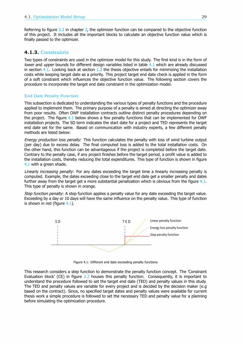
4.1. Optimization Model Setup 29
Referring to figure 2.2 in chapter 2, the optimizer function can be compared to the objective functionof this project. It includes all the important blocks to calculate an objective function value which isfinally passed to the optimizer.
4.1.3. ConstraintsTwo types of constraints are used in the optimizer model for this study. The first kind is in the form oflower and upper bounds for different design variables listed in table 4.1 which are already discussedin section 4.1. Looking back at section 1.2 the thesis objective entails for minimizing the installationcosts while keeping target date as a priority. This project target end date check is applied in the formof a soft constraint which influences the objective function value. The following section covers theprocedure to incorporate the target end date constraint in the optimization model.
End Date Penalty Function
This subsection is dedicated to understanding the various types of penalty functions and the procedureapplied to implement them. The primary purpose of a penalty is aimed at directing the optimizer awayfrom poor results. Often OWF installation contracts outline distinct penalty procedures depending onthe project. The figure 4.1 below shows a few penalty functions that can be implemented for OWFinstallation projects. The SD term indicates the start date for a project and TED represents the targetend date set for the same. Based on communication with industry experts, a few different penaltymethods are listed below:
Energy production loss penalty: This function calculates the penalty with loss of wind turbine output(per day) due to excess delay. The final computed loss is added to the total installation costs. Onthe other hand, this function can be advantageous if the project is completed before the target date.Contrary to the penalty case, if any project finishes before the target period, a profit value is added tothe installation costs, thereby reducing the total expenditures. This type of function is shown in figure4.1 with a green shade.
Linearly increasing penalty: For any dates exceeding the target time a linearly increasing penalty iscomputed. Example, the dates exceeding close to the target end date get a smaller penalty and datesfurther away from the target get a more substantial penalization which is obvious from the figure 4.1.This type of penalty is shown in orange.
Step function penalty: A step function applies a penalty value for any date exceeding the target value.Exceeding by a day or 10 days will have the same influence on the penalty value. This type of functionis shown in red (figure 4.1).
Figure 4.1: Different end date exceeding penalty functions
This research considers a step function to demonstrate the penalty function concept. The ’ConstraintEvaluation block’ (CE) in figure 2.2 houses this penalty function. Consequently, it is important tounderstand the procedure followed to set the target end date (TED) and penalty values in this study.The TED and penalty values are variable for every project and is decided by the decision maker (e.gbased on the contract). Since, no specified target dates and penalty values were available for currentthesis work a simple procedure is followed to set the necessary TED and penalty value for a planningbefore simulating the optimization procedure.
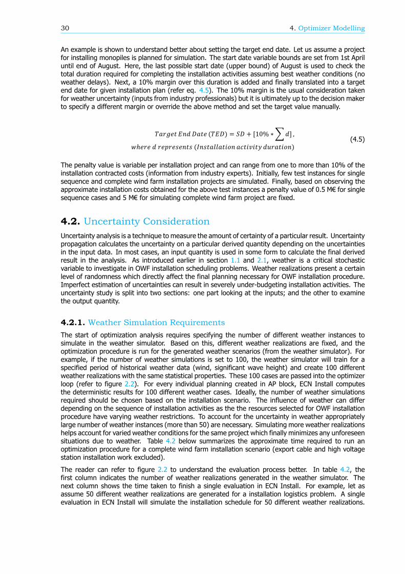
30 4. Optimizer Modelling
An example is shown to understand better about setting the target end date. Let us assume a projectfor installing monopiles is planned for simulation. The start date variable bounds are set from 1st Apriluntil end of August. Here, the last possible start date (upper bound) of August is used to check thetotal duration required for completing the installation activities assuming best weather conditions (noweather delays). Next, a 10% margin over this duration is added and finally translated into a targetend date for given installation plan (refer eq. 4.5). The 10% margin is the usual consideration takenfor weather uncertainty (inputs from industry professionals) but it is ultimately up to the decision makerto specify a different margin or override the above method and set the target value manually.
𝑇𝑎𝑟𝑔𝑒𝑡 𝐸𝑛𝑑 𝐷𝑎𝑡𝑒 (𝑇𝐸𝐷) = 𝑆𝐷 + [10% ∗∑𝑑] ,𝑤ℎ𝑒𝑟𝑒 𝑑 𝑟𝑒𝑝𝑟𝑒𝑠𝑒𝑛𝑡𝑠 (𝐼𝑛𝑠𝑡𝑎𝑙𝑙𝑎𝑡𝑖𝑜𝑛 𝑎𝑐𝑡𝑖𝑣𝑖𝑡𝑦 𝑑𝑢𝑟𝑎𝑡𝑖𝑜𝑛)
(4.5)
The penalty value is variable per installation project and can range from one to more than 10% of theinstallation contracted costs (information from industry experts). Initially, few test instances for singlesequence and complete wind farm installation projects are simulated. Finally, based on observing theapproximate installation costs obtained for the above test instances a penalty value of 0.5 M€ for singlesequence cases and 5 M€ for simulating complete wind farm project are fixed.
4.2. Uncertainty ConsiderationUncertainty analysis is a technique to measure the amount of certainty of a particular result. Uncertaintypropagation calculates the uncertainty on a particular derived quantity depending on the uncertaintiesin the input data. In most cases, an input quantity is used in some form to calculate the final derivedresult in the analysis. As introduced earlier in section 1.1 and 2.1, weather is a critical stochasticvariable to investigate in OWF installation scheduling problems. Weather realizations present a certainlevel of randomness which directly affect the final planning necessary for OWF installation procedure.Imperfect estimation of uncertainties can result in severely under-budgeting installation activities. Theuncertainty study is split into two sections: one part looking at the inputs; and the other to examinethe output quantity.
4.2.1. Weather Simulation RequirementsThe start of optimization analysis requires specifying the number of different weather instances tosimulate in the weather simulator. Based on this, different weather realizations are fixed, and theoptimization procedure is run for the generated weather scenarios (from the weather simulator). Forexample, if the number of weather simulations is set to 100, the weather simulator will train for aspecified period of historical weather data (wind, significant wave height) and create 100 differentweather realizations with the same statistical properties. These 100 cases are passed into the optimizerloop (refer to figure 2.2). For every individual planning created in AP block, ECN Install computesthe deterministic results for 100 different weather cases. Ideally, the number of weather simulationsrequired should be chosen based on the installation scenario. The influence of weather can differdepending on the sequence of installation activities as the the resources selected for OWF installationprocedure have varying weather restrictions. To account for the uncertainty in weather appropriatelylarge number of weather instances (more than 50) are necessary. Simulating more weather realizationshelps account for varied weather conditions for the same project which finally minimizes any unforeseensituations due to weather. Table 4.2 below summarizes the approximate time required to run anoptimization procedure for a complete wind farm installation scenario (export cable and high voltagestation installation work excluded).
The reader can refer to figure 2.2 to understand the evaluation process better. In table 4.2, thefirst column indicates the number of weather realizations generated in the weather simulator. Thenext column shows the time taken to finish a single evaluation in ECN Install. For example, let asassume 50 different weather realizations are generated for a installation logistics problem. A singleevaluation in ECN Install will simulate the installation schedule for 50 different weather realizations.

4.2. Uncertainty Consideration 31
No. of weathersimulations
Single ECN Installevaluation (s)
Total uniqueevaluations Total time (hr)
200 916 1500 34.8150 747 1500 28.8100 490 1500 20.170 335 1500 14.650 233 1500 11.1
Table 4.2: Optimization time vs Number of weather simulations
The time taken to simulate these 50 weather scenarios in ECN Install is 233 seconds (See table). Thisnumber increases linearly with increasing number of weather simulations, as installation results needto be calculated for more weather realizations. In the new architecture ECN Install is integrated withan optimization procedure. Hence, every individual combination of design variables translate to newinstallation schedule which is evaluated in ECN Install (one unique evaluation). Test runs reveal thatthe total number of unique evaluations of ECN Install inside the optimization process never exceed1500 counts. Hence, this value is taken as a benchmark for calculating the total optimization analysistime. The last column finally displays the total optimization time in hours assuming all optimizationcomputations are done with 12 parallel cores on ECN cluster. In this research, the weather simulationsare capped at 100 different realizations due to limited availability of ECN cluster. The next section givesa run through of the process followed for uncertainty consideration at ECN Install output.
4.2.2. ECN Install Output AnalysisThe previous section elucidates on an exact number of weather realizations run in ECN Install. Lookingback at figure 2.2, the uncertainty consideration block indicated in the figure is covered here. Figure4.2 below shows the process flow of output from ECN Install to the optimizer.
Figure 4.2: ECN Install output uncertainty handling
𝐶 = [𝑐 + 𝑝(𝑓)] (4.6)
𝑦 = 1𝑛𝑠𝑖𝑚 ∑ 𝐶 (4.7)
Based on the reasoning from previous section, we see that ECN Install provides results for 100 differentweather realizations. This number of weather realizations is represented by nsim term in the objectivefunction (equation 4.4). Let us understand the final value calculation process with the help of equations4.6 and 4.7. The subscript i in the above equations represent the unique weather simulation number.First, the results for total installation costs and end dates required for the study are extracted from ECNInstall output file. Next, the end dates f are passed through a function p() to evaluate the end dateexceedance (see section 4.1.3). Once this is complete, a total cost C is obtained for all the individual
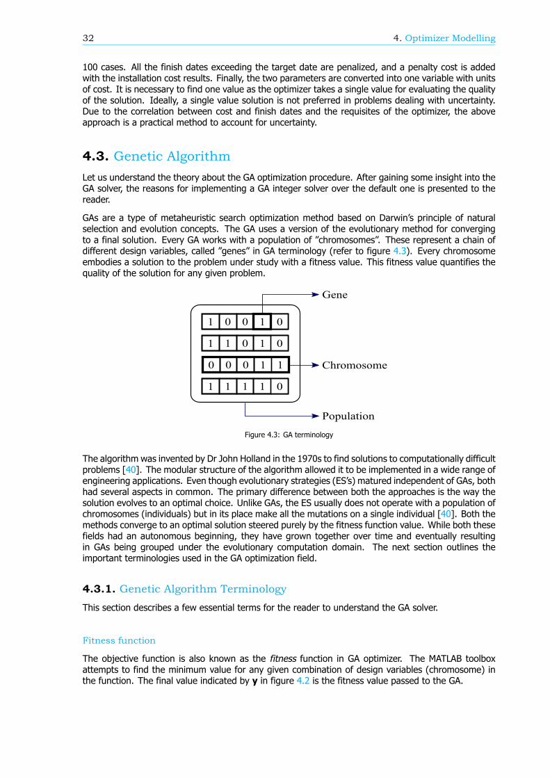
32 4. Optimizer Modelling
100 cases. All the finish dates exceeding the target date are penalized, and a penalty cost is addedwith the installation cost results. Finally, the two parameters are converted into one variable with unitsof cost. It is necessary to find one value as the optimizer takes a single value for evaluating the qualityof the solution. Ideally, a single value solution is not preferred in problems dealing with uncertainty.Due to the correlation between cost and finish dates and the requisites of the optimizer, the aboveapproach is a practical method to account for uncertainty.
4.3. Genetic AlgorithmLet us understand the theory about the GA optimization procedure. After gaining some insight into theGA solver, the reasons for implementing a GA integer solver over the default one is presented to thereader.
GAs are a type of metaheuristic search optimization method based on Darwin’s principle of naturalselection and evolution concepts. The GA uses a version of the evolutionary method for convergingto a final solution. Every GA works with a population of ”chromosomes”. These represent a chain ofdifferent design variables, called ”genes” in GA terminology (refer to figure 4.3). Every chromosomeembodies a solution to the problem under study with a fitness value. This fitness value quantifies thequality of the solution for any given problem.
1 1 0 1 0
1 0 0 1 0
0 0 0 1 1
1 1 1 1 0
Gene
Chromosome
Population
Figure 4.3: GA terminology
The algorithm was invented by Dr John Holland in the 1970s to find solutions to computationally difficultproblems [40]. The modular structure of the algorithm allowed it to be implemented in a wide range ofengineering applications. Even though evolutionary strategies (ES’s) matured independent of GAs, bothhad several aspects in common. The primary difference between both the approaches is the way thesolution evolves to an optimal choice. Unlike GAs, the ES usually does not operate with a population ofchromosomes (individuals) but in its place make all the mutations on a single individual [40]. Both themethods converge to an optimal solution steered purely by the fitness function value. While both thesefields had an autonomous beginning, they have grown together over time and eventually resultingin GAs being grouped under the evolutionary computation domain. The next section outlines theimportant terminologies used in the GA optimization field.
4.3.1. Genetic Algorithm Terminology
This section describes a few essential terms for the reader to understand the GA solver.
Fitness function
The objective function is also known as the fitness function in GA optimizer. The MATLAB toolboxattempts to find the minimum value for any given combination of design variables (chromosome) inthe function. The final value indicated by y in figure 4.2 is the fitness value passed to the GA.
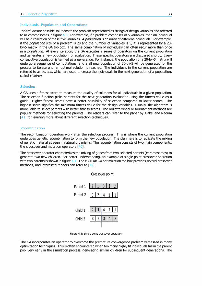
4.3. Genetic Algorithm 33
Individuals, Population and Generations
Individuals are possible solutions to the problem represented as strings of design variables and referredto as chromosomes in figure 4.3. For example, if a problem comprises of 5 variables, then an individualwill be a collection of these five variables. A population is an array of different individuals. For example,if the population size of a problem is 20 and the number of variables is 5, it is represented by a 20-by-5 matrix in the GA toolbox. The same combination of individuals can often recur more than oncein a population. At every iteration, the GA executes a series of operators on the current populationand generates a new population for evaluation. These specific operators are discussed shortly. Everyconsecutive population is termed as a generation. For instance, the population of a 20-by-5 matrix willundergo a sequence of computations, and a all new population of 20-by-5 will be generated for theprocess to iterate until an optimal solution is reached. The individuals in the current population arereferred to as parents which are used to create the individuals in the next generation of a population,called children.
Selection
A GA uses a fitness score to measure the quality of solutions for all individuals in a given population.The selection function picks parents for the next generation evaluation using the fitness value as aguide. Higher fitness scores have a better possibility of selection compared to lower scores. Thehighest score signifies the minimum fitness value for the design variables. Usually, the algorithm ismore liable to select parents with better fitness scores. The roulette wheel or tournament methods arepopular methods for selecting the parents. The readers can refer to the paper by Alabsi and Naoum[41] for learning more about different selection techniques.
Recombination
The recombination operators work after the selection process. This is where the current populationundergoes genetic recombination to form the new population. The plan here is to replicate the mixingof genetic material as seen in natural organisms. The recombination consists of two main components,the crossover and mutation operators [40].
The crossover operator characterizes the mixing of genes from two selected parents (chromosomes) togenerate two new children. For better understanding, an example of single point crossover operationwith two parents is shown in figure 4.4. The MATLAB GA optimization toolbox provides several crossovermethods, and interested readers can refer to [42].
Figure 4.4: single point crossover operation
The GA incorporates an operator to overcome the premature convergence problem witnessed in manyoptimization techniques. This is often encountered when too many highly fit individuals fall in the parentpool very early in the simulation process, generating similar children for subsequent generations. The
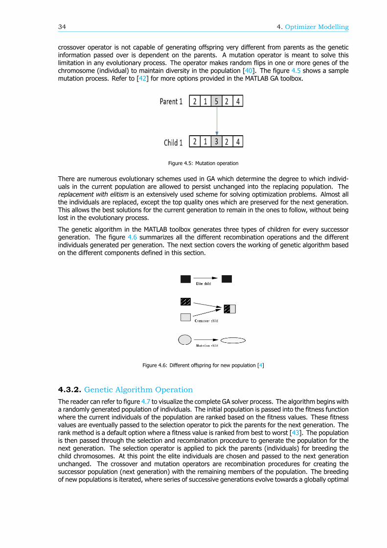
34 4. Optimizer Modelling
crossover operator is not capable of generating offspring very different from parents as the geneticinformation passed over is dependent on the parents. A mutation operator is meant to solve thislimitation in any evolutionary process. The operator makes random flips in one or more genes of thechromosome (individual) to maintain diversity in the population [40]. The figure 4.5 shows a samplemutation process. Refer to [42] for more options provided in the MATLAB GA toolbox.
Figure 4.5: Mutation operation
There are numerous evolutionary schemes used in GA which determine the degree to which individ-uals in the current population are allowed to persist unchanged into the replacing population. Thereplacement with elitism is an extensively used scheme for solving optimization problems. Almost allthe individuals are replaced, except the top quality ones which are preserved for the next generation.This allows the best solutions for the current generation to remain in the ones to follow, without beinglost in the evolutionary process.
The genetic algorithm in the MATLAB toolbox generates three types of children for every successorgeneration. The figure 4.6 summarizes all the different recombination operations and the differentindividuals generated per generation. The next section covers the working of genetic algorithm basedon the different components defined in this section.
Figure 4.6: Different offspring for new population [4]
4.3.2. Genetic Algorithm OperationThe reader can refer to figure 4.7 to visualize the complete GA solver process. The algorithm begins witha randomly generated population of individuals. The initial population is passed into the fitness functionwhere the current individuals of the population are ranked based on the fitness values. These fitnessvalues are eventually passed to the selection operator to pick the parents for the next generation. Therank method is a default option where a fitness value is ranked from best to worst [43]. The populationis then passed through the selection and recombination procedure to generate the population for thenext generation. The selection operator is applied to pick the parents (individuals) for breeding thechild chromosomes. At this point the elite individuals are chosen and passed to the next generationunchanged. The crossover and mutation operators are recombination procedures for creating thesuccessor population (next generation) with the remaining members of the population. The breedingof new populations is iterated, where series of successive generations evolve towards a globally optimal
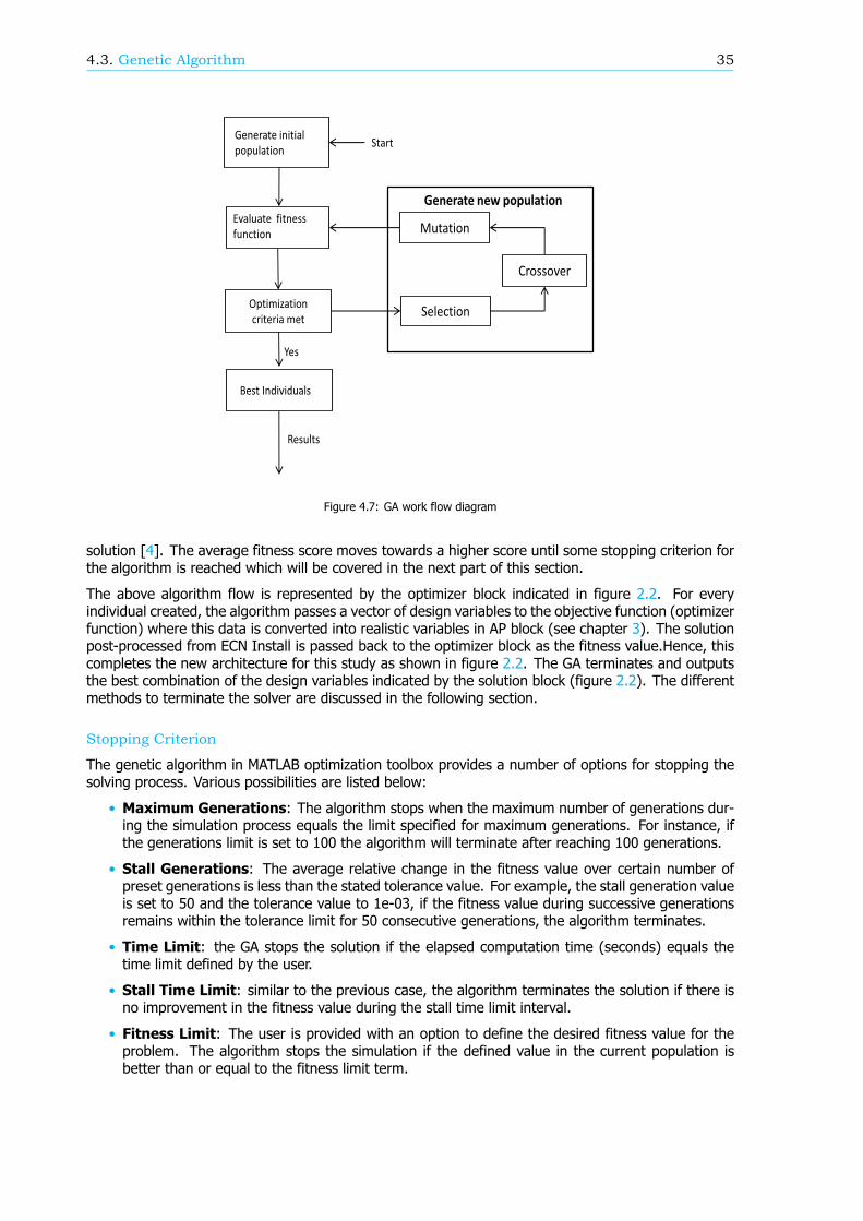
4.3. Genetic Algorithm 35
Figure 4.7: GA work flow diagram
solution [4]. The average fitness score moves towards a higher score until some stopping criterion forthe algorithm is reached which will be covered in the next part of this section.
The above algorithm flow is represented by the optimizer block indicated in figure 2.2. For everyindividual created, the algorithm passes a vector of design variables to the objective function (optimizerfunction) where this data is converted into realistic variables in AP block (see chapter 3). The solutionpost-processed from ECN Install is passed back to the optimizer block as the fitness value.Hence, thiscompletes the new architecture for this study as shown in figure 2.2. The GA terminates and outputsthe best combination of the design variables indicated by the solution block (figure 2.2). The differentmethods to terminate the solver are discussed in the following section.
Stopping Criterion
The genetic algorithm in MATLAB optimization toolbox provides a number of options for stopping thesolving process. Various possibilities are listed below:
• Maximum Generations: The algorithm stops when the maximum number of generations dur-ing the simulation process equals the limit specified for maximum generations. For instance, ifthe generations limit is set to 100 the algorithm will terminate after reaching 100 generations.
• Stall Generations: The average relative change in the fitness value over certain number ofpreset generations is less than the stated tolerance value. For example, the stall generation valueis set to 50 and the tolerance value to 1e-03, if the fitness value during successive generationsremains within the tolerance limit for 50 consecutive generations, the algorithm terminates.
• Time Limit: the GA stops the solution if the elapsed computation time (seconds) equals thetime limit defined by the user.
• Stall Time Limit: similar to the previous case, the algorithm terminates the solution if there isno improvement in the fitness value during the stall time limit interval.
• Fitness Limit: The user is provided with an option to define the desired fitness value for theproblem. The algorithm stops the simulation if the defined value in the current population isbetter than or equal to the fitness limit term.

36 4. Optimizer Modelling
The algorithm discontinues the simulation if any one of the above defined conditions are met. The usercan define specific stopping criteria based on the problem type and instruct the optimizer to ignore thedefault limits.
4.3.3. MATLAB GA Integer Solver
The default MATLAB GA solver utilizes a continuous variable range for the optimization process. Sadly,the design variables for our problem cannot be implemented in the optimization solver in its defaultsetup. Section 4.1 covers the different design variables used in the research work to confirm theabove point. Notably, all the design variables in this study are discrete. This requires the optimizerto evaluate only integer choices and exclude all other cases. Fortunately, the GA solver provides theoption of integer solver for such design variables. This part encapsulates the modifications in the GAinteger solver over the default toolbox algorithm.
• Double(natural numbers) vector population type as referred in MATLAB toolbox is used over thedefault bit string(binary numbers) option. The difference between double vector representationand bit string representation is shown in figure 4.8. The optimizer solves faster with this restric-tion as the integer bounds are managed with ease when the individuals in population are alsorepresented in similar format.
• The solver utilizes the binary tournament choice as the option in the selection operator step. Inthis method two parents are selected randomly from the current generation and the one withsuperior score is picked as the parent.
• To enforce variables to be integers the algorithm uses a distinctive creation, crossover and mu-tation function. For more details about the functions refer to Deep et al [44].
• Unlike the default case, where the fitness value is used as a guide for finding the best option, apenalty function is used as reference within the integer solver. The penalty function is developedto restrict the optimizer to select only integer variable solutions in the algorithm. It is combinedwith the binary tournament selection function to pick individuals for later generations. If theindividual is feasible, the penalty value is used as the fitness value. Else the member is rankedlast among the in-feasible individuals in the population and discarded.
Figure 4.8: Design variable (DV) representation in GA population
Even though the integer GA solver demands using fixed selection and recombination operators theadvantages outweigh the limitations. The manual implementation of integer constraining the variablesis time-consuming and susceptible to random modeling error. Hence, it makes a logical argument touse the in-built solver provided in MATLAB toolbox.
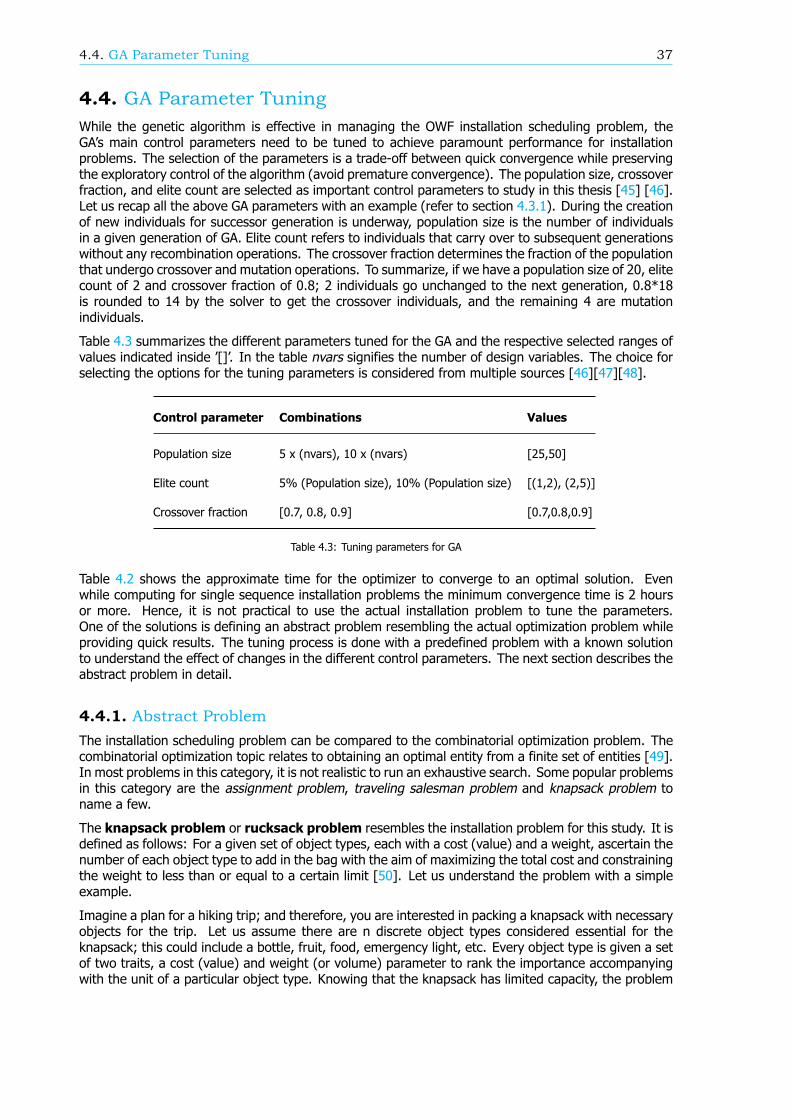
4.4. GA Parameter Tuning 37
4.4. GA Parameter TuningWhile the genetic algorithm is effective in managing the OWF installation scheduling problem, theGA’s main control parameters need to be tuned to achieve paramount performance for installationproblems. The selection of the parameters is a trade-off between quick convergence while preservingthe exploratory control of the algorithm (avoid premature convergence). The population size, crossoverfraction, and elite count are selected as important control parameters to study in this thesis [45] [46].Let us recap all the above GA parameters with an example (refer to section 4.3.1). During the creationof new individuals for successor generation is underway, population size is the number of individualsin a given generation of GA. Elite count refers to individuals that carry over to subsequent generationswithout any recombination operations. The crossover fraction determines the fraction of the populationthat undergo crossover and mutation operations. To summarize, if we have a population size of 20, elitecount of 2 and crossover fraction of 0.8; 2 individuals go unchanged to the next generation, 0.8*18is rounded to 14 by the solver to get the crossover individuals, and the remaining 4 are mutationindividuals.
Table 4.3 summarizes the different parameters tuned for the GA and the respective selected ranges ofvalues indicated inside ’[]’. In the table nvars signifies the number of design variables. The choice forselecting the options for the tuning parameters is considered from multiple sources [46][47][48].
Control parameter Combinations Values
Population size 5 x (nvars), 10 x (nvars) [25,50]
Elite count 5% (Population size), 10% (Population size) [(1,2), (2,5)]
Crossover fraction [0.7, 0.8, 0.9] [0.7,0.8,0.9]
Table 4.3: Tuning parameters for GA
Table 4.2 shows the approximate time for the optimizer to converge to an optimal solution. Evenwhile computing for single sequence installation problems the minimum convergence time is 2 hoursor more. Hence, it is not practical to use the actual installation problem to tune the parameters.One of the solutions is defining an abstract problem resembling the actual optimization problem whileproviding quick results. The tuning process is done with a predefined problem with a known solutionto understand the effect of changes in the different control parameters. The next section describes theabstract problem in detail.
4.4.1. Abstract ProblemThe installation scheduling problem can be compared to the combinatorial optimization problem. Thecombinatorial optimization topic relates to obtaining an optimal entity from a finite set of entities [49].In most problems in this category, it is not realistic to run an exhaustive search. Some popular problemsin this category are the assignment problem, traveling salesman problem and knapsack problem toname a few.
The knapsack problem or rucksack problem resembles the installation problem for this study. It isdefined as follows: For a given set of object types, each with a cost (value) and a weight, ascertain thenumber of each object type to add in the bag with the aim of maximizing the total cost and constrainingthe weight to less than or equal to a certain limit [50]. Let us understand the problem with a simpleexample.
Imagine a plan for a hiking trip; and therefore, you are interested in packing a knapsack with necessaryobjects for the trip. Let us assume there are n discrete object types considered essential for theknapsack; this could include a bottle, fruit, food, emergency light, etc. Every object type is given a setof two traits, a cost (value) and weight (or volume) parameter to rank the importance accompanyingwith the unit of a particular object type. Knowing that the knapsack has limited capacity, the problem

38 4. Optimizer Modelling
requires filling the sack with the optimal combination of specific object types which maximizes the costvalue. The above example describes the simple knapsack problem case, let us see how this can bemodified to represent the problem in this dissertation.
The 0/1 knapsack problem is a subset of the knapsack problem category. It differentiates from theusual knapsack problem regarding the number of objects selected per type. In the 0/1 knapsackproblem case the number of object types are restricted to 1 or 0. The 0/1 knapsack problem is slightlycustomized for building the abstract problem for tuning the optimizer parameters. The customizationis done for two aspects. First, in the default 0/1 knapsack problem one or nil option is selected perobject type, whereas, in our problem one option per object type must be always picked. So, lookingback at the above example, the default 0/1 knapsack problem may or may not include a bottle fromthe bottle type object for the hiking trip. But, for our problem it is a must that one bottle is picked forthe trip. Secondly, the cost maximization problem for the default 0/1 knapsack problem is changed toa minimization problem for our case.
Let us assume set of 𝑘 object types, with a weight 𝑤 and cost value 𝑣 , constrained by maximumweight capacity 𝑊 for the knapsack problem. 𝑗 represents the data for every unique object per type.Refer to figure 4.9 to visualize the problem representation in GA showing the different design variables.
𝑦 = 𝑀𝑖𝑛𝑖𝑚𝑖𝑧𝑒 ∑𝑣 (4.8)
𝑆𝑢𝑏𝑗𝑒𝑐𝑡 𝑡𝑜 ∶ ∑𝑤 <= 𝑊 (4.9)
Figure 4.9: Knapsack problem representation in GA
The equations 4.8 and 4.9 constitute the objective and constraint for the knapsack problem. Thefollowing steps describe the problem implementation in GA solver:
Step 1: A knapsack of fixed capacity considered for the abstract problem. Represent the design vari-ables of a single sequence installation activity as objects in the abstract problem.
Step 2: Next the number of object types for the knapsack is fixed. A Single sequence installationproblem at max incorporates five design variables in this study. Hence, in GA double (naturalnumbers) string type with five variables is created for the abstract problem.
Step 3: Next, a list of options for the different object types are created. The options per object typecan be visualized in figure 4.9.
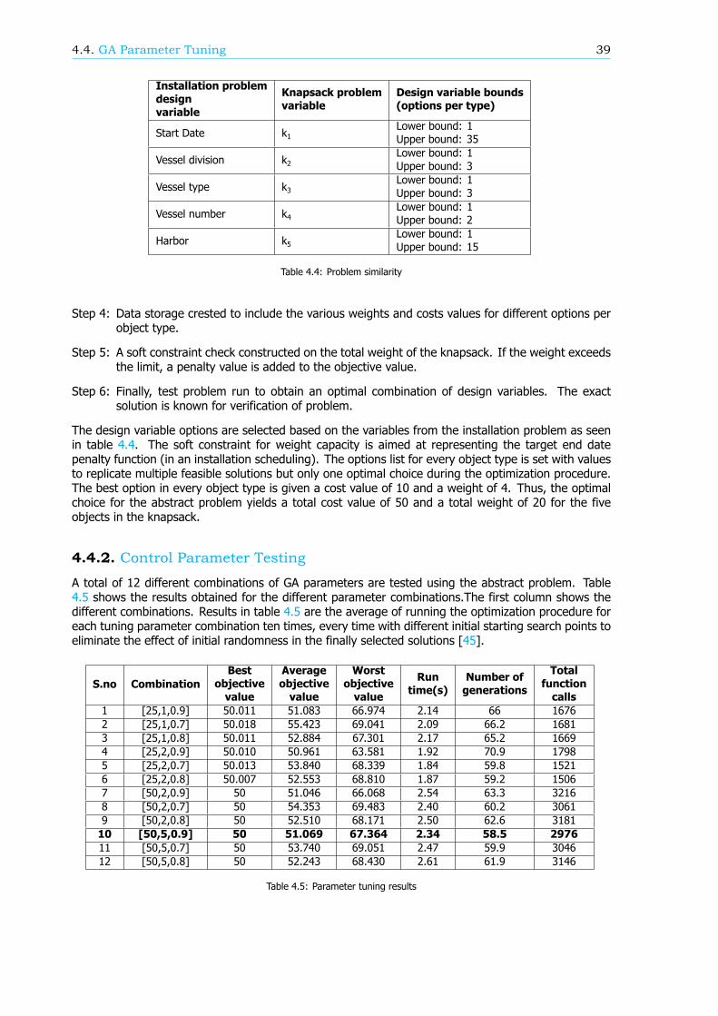
4.4. GA Parameter Tuning 39
Installation problemdesignvariable
Knapsack problemvariable
Design variable bounds(options per type)
Start Date k1Lower bound: 1Upper bound: 35
Vessel division k2Lower bound: 1Upper bound: 3
Vessel type k3Lower bound: 1Upper bound: 3
Vessel number k4Lower bound: 1Upper bound: 2
Harbor k5Lower bound: 1Upper bound: 15
Table 4.4: Problem similarity
Step 4: Data storage crested to include the various weights and costs values for different options perobject type.
Step 5: A soft constraint check constructed on the total weight of the knapsack. If the weight exceedsthe limit, a penalty value is added to the objective value.
Step 6: Finally, test problem run to obtain an optimal combination of design variables. The exactsolution is known for verification of problem.
The design variable options are selected based on the variables from the installation problem as seenin table 4.4. The soft constraint for weight capacity is aimed at representing the target end datepenalty function (in an installation scheduling). The options list for every object type is set with valuesto replicate multiple feasible solutions but only one optimal choice during the optimization procedure.The best option in every object type is given a cost value of 10 and a weight of 4. Thus, the optimalchoice for the abstract problem yields a total cost value of 50 and a total weight of 20 for the fiveobjects in the knapsack.
4.4.2. Control Parameter Testing
A total of 12 different combinations of GA parameters are tested using the abstract problem. Table4.5 shows the results obtained for the different parameter combinations.The first column shows thedifferent combinations. Results in table 4.5 are the average of running the optimization procedure foreach tuning parameter combination ten times, every time with different initial starting search points toeliminate the effect of initial randomness in the finally selected solutions [45].
S.no CombinationBest
objectivevalue
Averageobjectivevalue
Worstobjectivevalue
Runtime(s)
Number ofgenerations
Totalfunctioncalls
1 [25,1,0.9] 50.011 51.083 66.974 2.14 66 16762 [25,1,0.7] 50.018 55.423 69.041 2.09 66.2 16813 [25,1,0.8] 50.011 52.884 67.301 2.17 65.2 16694 [25,2,0.9] 50.010 50.961 63.581 1.92 70.9 17985 [25,2,0.7] 50.013 53.840 68.339 1.84 59.8 15216 [25,2,0.8] 50.007 52.553 68.810 1.87 59.2 15067 [50,2,0.9] 50 51.046 66.068 2.54 63.3 32168 [50,2,0.7] 50 54.353 69.483 2.40 60.2 30619 [50,2,0.8] 50 52.510 68.171 2.50 62.6 318110 [50,5,0.9] 50 51.069 67.364 2.34 58.5 297611 [50,5,0.7] 50 53.740 69.051 2.47 59.9 304612 [50,5,0.8] 50 52.243 68.430 2.61 61.9 3146
Table 4.5: Parameter tuning results
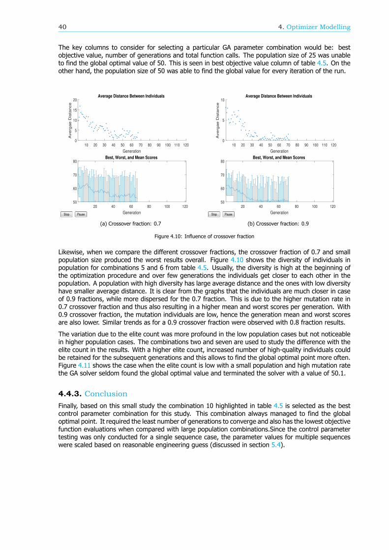
40 4. Optimizer Modelling
The key columns to consider for selecting a particular GA parameter combination would be: bestobjective value, number of generations and total function calls. The population size of 25 was unableto find the global optimal value of 50. This is seen in best objective value column of table 4.5. On theother hand, the population size of 50 was able to find the global value for every iteration of the run.
10 20 30 40 50 60 70 80 90 100 110 120
Generation
0
5
10
15
20
Ave
rga
e D
ista
nce
Average Distance Between Individuals
20 40 60 80 100 120
Generation
50
60
70
80Best, Worst, and Mean Scores
PauseStop
(a) Crossover fraction: 0.7
10 20 30 40 50 60 70 80 90 100 110 120
Generation
0
5
10
Ave
rga
e D
ista
nce
Average Distance Between Individuals
20 40 60 80 100 120
Generation
50
60
70
80Best, Worst, and Mean Scores
PauseStop
(b) Crossover fraction: 0.9
Figure 4.10: Influence of crossover fraction
Likewise, when we compare the different crossover fractions, the crossover fraction of 0.7 and smallpopulation size produced the worst results overall. Figure 4.10 shows the diversity of individuals inpopulation for combinations 5 and 6 from table 4.5. Usually, the diversity is high at the beginning ofthe optimization procedure and over few generations the individuals get closer to each other in thepopulation. A population with high diversity has large average distance and the ones with low diversityhave smaller average distance. It is clear from the graphs that the individuals are much closer in caseof 0.9 fractions, while more dispersed for the 0.7 fraction. This is due to the higher mutation rate in0.7 crossover fraction and thus also resulting in a higher mean and worst scores per generation. With0.9 crossover fraction, the mutation individuals are low, hence the generation mean and worst scoresare also lower. Similar trends as for a 0.9 crossover fraction were observed with 0.8 fraction results.
The variation due to the elite count was more profound in the low population cases but not noticeablein higher population cases. The combinations two and seven are used to study the difference with theelite count in the results. With a higher elite count, increased number of high-quality individuals couldbe retained for the subsequent generations and this allows to find the global optimal point more often.Figure 4.11 shows the case when the elite count is low with a small population and high mutation ratethe GA solver seldom found the global optimal value and terminated the solver with a value of 50.1.
4.4.3. ConclusionFinally, based on this small study the combination 10 highlighted in table 4.5 is selected as the bestcontrol parameter combination for this study. This combination always managed to find the globaloptimal point. It required the least number of generations to converge and also has the lowest objectivefunction evaluations when compared with large population combinations.Since the control parametertesting was only conducted for a single sequence case, the parameter values for multiple sequenceswere scaled based on reasonable engineering guess (discussed in section 5.4).
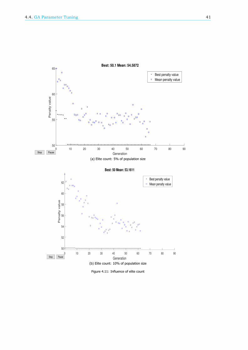
4.4. GA Parameter Tuning 41
0 10 20 30 40 50 60 70 80 90
Generation
50
55
60
65
Pe
na
lty v
alu
e
Best: 50.1 Mean: 54.5872
Best penalty value
Mean penalty value
PauseStop
(a) Elite count: 5% of population size
0 10 20 30 40 50 60 70 80 90
Generation
50
52
54
56
58
60
62
Penalty v
alu
e
Best: 50 Mean: 53.1611
Best penalty value
Mean penalty value
PauseStop
(b) Elite count: 10% of population size
Figure 4.11: Influence of elite count


5Case Study
This chapter describes the case studies that were performed with the installation optimization set-uptowards answering the thesis objective defined in section 1.2. The first section introduces the locationused for simulating the case studies. A brief overview of the OWF market of Europe is given to thereader. This later allows formulating the various cases for this study. A set of 2 case studies are runto investigate the working of the optimizer with ECN Install in solving installation scheduling problems.The first case examines the optimizer choices based on variable input scenarios. This case comprises of3 sets of single sequence activities to understand the different design variable choices and significanceof target end date in the projects. The second case is extended for a more complex problem, where acomplete wind farm installation is studied. It covers multiple sequence activities and its influence onthe optimizer decisions.
5.1. OWF locationThe case studies for this thesis study are investigated for the Borssele Wind Farm Zone (BWFZ) [5]. Itis located in the southern part of the Dutch Exclusive Economic Zone (EEZ), shown in figure 5.1 below.
Figure 5.1: Borssele wind farm zone [5]
20 years of historical wind and wave data for the wind farm zone is collected and utilized as a fixed inputfor all the case studies. BWFZ is split into four wind farms which will account for a total capacity of 1400MW. This location is used for constructing hypothetical wind farm installation scenarios to highlight theoptimizer working with ECN Install. The location coordinates for wind farm zone I and II are acquiredand set for all case studies in this chapter [51].
43
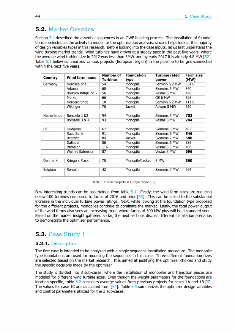
44 5. Case Study
5.2. Market OverviewSection 3.4 described the essential sequences in an OWF building process. The installation of founda-tions is selected as the activity to model for the optimization analysis, since it helps look at the majorityof design variables types in this research. Before looking into the case inputs, let us first understand thewind turbine market trends. Wind turbines have grown at a steady pace in the past five years, wherethe average wind turbine size in 2012 was less than 3MW, and by early 2017 it is already 4.8 MW [52].Table 5.1 below summarizes various projects (European region) in the pipeline to be grid-connectedwithin the next five years.
Country Wind farm nameNumber ofTurbines
Foundationtype
Turbine ratedpower
Farm size(MW)
Germany Nordsee one 54 Monopile Senvion 6.2 MW 334.8Arkona 60 Monopile Siemens 6 MW 360Borkum Riffgrund 2 56 Monopile Vestas 8 MW 448Merkur 66 Monopile GE 6 MW 396Nordergrunde 18 Monopile Senvion 6.2 MW 111.6Wikinger 70 Jacket Adwen 5 MW 350
Netherlands Borssele 1 &2 94 Monopile Siemens 8 MW 752Borssele 3 & 4 93 Monopile Vestas 8 MW 744
UK Dudgeon 67 Monopile Siemens 6 MW 402Race Bank 91 Monopile Siemens 6 MW 546Beatrice 84 Jacket Siemens 7 MW 588Galloper 56 Monopile Siemens 6 MW 336Rampion 116 Monopile Vestas 3.5 MW 406Walney Extension 87 Monopile Vestas 8 MW 696
Denmark Kriegers Flack 70 Monopile/Jacket 8 MW 560
Belgium Rentel 42 Monopile Siemens 7 MW 294
Table 5.1: New projects in Europe region [6]
Few interesting trends can be ascertained from table 5.1. Firstly, the wind farm sizes are reducingbelow 100 turbines compared to farms of 2016 and prior [53]. This can be linked to the substantialincrease in the individual turbine power ratings. Next, while looking at the foundation type proposedfor the different projects, monopiles continue to dominate the market. Lastly, the total power outputof the wind farms also sees an increasing trend where farms of 500 MW plus will be a standard soon.Based on the market insight gathered so far, the next sections discuss different installation scenariosto demonstrate the optimizer performance.
5.3. Case Study 15.3.1. DescriptionThe first case is intended to be analyzed with a single sequence installation procedure. The monopiletype foundations are used for modeling the sequences in this case. Three different foundation sizesare selected based on the market research. It is aimed at justifying the optimizer choices and studythe specific decisions made by the optimizer.
The study is divided into 3 sub-cases, where the installation of monopiles and transition pieces aremodeled for different wind turbine sizes. Even though the weight parameters for the foundations arelocation specific, table 5.2 considers average values from previous projects for cases 1A and 1B [6].The values for case 1C are calculated from [54]. Table 5.3 summarizes the optimizer design variablesand control parameters utilized for the 3 sub-cases.
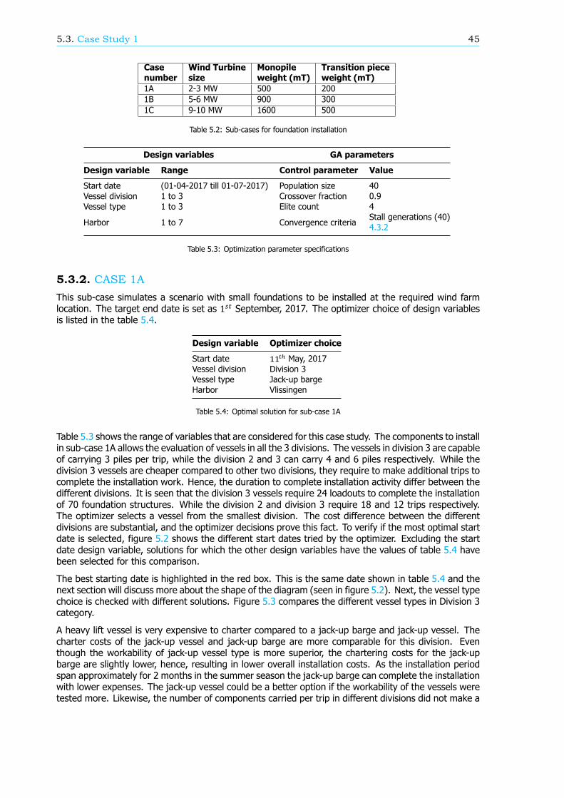
5.3. Case Study 1 45
Casenumber
Wind Turbinesize
Monopileweight (mT)
Transition pieceweight (mT)
1A 2-3 MW 500 2001B 5-6 MW 900 3001C 9-10 MW 1600 500
Table 5.2: Sub-cases for foundation installation
Design variables GA parameters
Design variable Range Control parameter Value
Start date (01-04-2017 till 01-07-2017) Population size 40Vessel division 1 to 3 Crossover fraction 0.9Vessel type 1 to 3 Elite count 4
Harbor 1 to 7 Convergence criteriaStall generations (40)4.3.2
Table 5.3: Optimization parameter specifications
5.3.2. CASE 1AThis sub-case simulates a scenario with small foundations to be installed at the required wind farmlocation. The target end date is set as 1 September, 2017. The optimizer choice of design variablesis listed in the table 5.4.
Design variable Optimizer choice
Start date May, 2017Vessel division Division 3Vessel type Jack-up bargeHarbor Vlissingen
Table 5.4: Optimal solution for sub-case 1A
Table 5.3 shows the range of variables that are considered for this case study. The components to installin sub-case 1A allows the evaluation of vessels in all the 3 divisions. The vessels in division 3 are capableof carrying 3 piles per trip, while the division 2 and 3 can carry 4 and 6 piles respectively. While thedivision 3 vessels are cheaper compared to other two divisions, they require to make additional trips tocomplete the installation work. Hence, the duration to complete installation activity differ between thedifferent divisions. It is seen that the division 3 vessels require 24 loadouts to complete the installationof 70 foundation structures. While the division 2 and division 3 require 18 and 12 trips respectively.The optimizer selects a vessel from the smallest division. The cost difference between the differentdivisions are substantial, and the optimizer decisions prove this fact. To verify if the most optimal startdate is selected, figure 5.2 shows the different start dates tried by the optimizer. Excluding the startdate design variable, solutions for which the other design variables have the values of table 5.4 havebeen selected for this comparison.
The best starting date is highlighted in the red box. This is the same date shown in table 5.4 and thenext section will discuss more about the shape of the diagram (seen in figure 5.2). Next, the vessel typechoice is checked with different solutions. Figure 5.3 compares the different vessel types in Division 3category.
A heavy lift vessel is very expensive to charter compared to a jack-up barge and jack-up vessel. Thecharter costs of the jack-up vessel and jack-up barge are more comparable for this division. Eventhough the workability of jack-up vessel type is more superior, the chartering costs for the jack-upbarge are slightly lower, hence, resulting in lower overall installation costs. As the installation periodspan approximately for 2 months in the summer season the jack-up barge can complete the installationwith lower expenses. The jack-up vessel could be a better option if the workability of the vessels weretested more. Likewise, the number of components carried per trip in different divisions did not make a
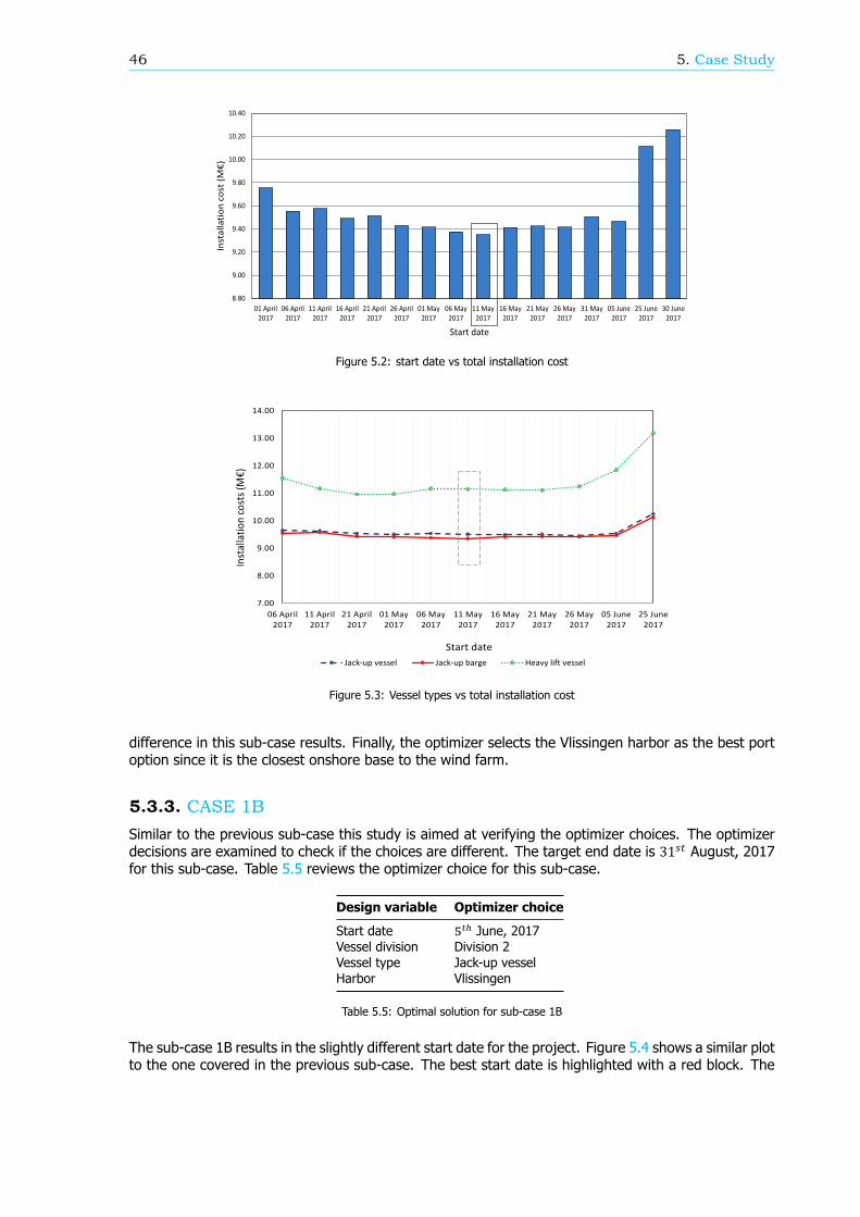
46 5. Case Study
Figure 5.2: start date vs total installation cost
Figure 5.3: Vessel types vs total installation cost
difference in this sub-case results. Finally, the optimizer selects the Vlissingen harbor as the best portoption since it is the closest onshore base to the wind farm.
5.3.3. CASE 1BSimilar to the previous sub-case this study is aimed at verifying the optimizer choices. The optimizerdecisions are examined to check if the choices are different. The target end date is 31 August, 2017for this sub-case. Table 5.5 reviews the optimizer choice for this sub-case.
Design variable Optimizer choice
Start date June, 2017Vessel division Division 2Vessel type Jack-up vesselHarbor Vlissingen
Table 5.5: Optimal solution for sub-case 1B
The sub-case 1B results in the slightly different start date for the project. Figure 5.4 shows a similar plotto the one covered in the previous sub-case. The best start date is highlighted with a red block. The
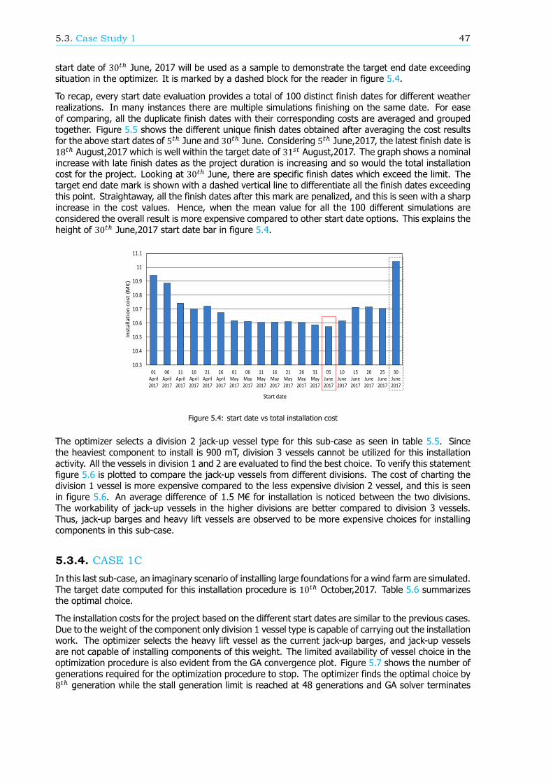
5.3. Case Study 1 47
start date of 30 June, 2017 will be used as a sample to demonstrate the target end date exceedingsituation in the optimizer. It is marked by a dashed block for the reader in figure 5.4.
To recap, every start date evaluation provides a total of 100 distinct finish dates for different weatherrealizations. In many instances there are multiple simulations finishing on the same date. For easeof comparing, all the duplicate finish dates with their corresponding costs are averaged and groupedtogether. Figure 5.5 shows the different unique finish dates obtained after averaging the cost resultsfor the above start dates of 5 June and 30 June. Considering 5 June,2017, the latest finish date is18 August,2017 which is well within the target date of 31 August,2017. The graph shows a nominalincrease with late finish dates as the project duration is increasing and so would the total installationcost for the project. Looking at 30 June, there are specific finish dates which exceed the limit. Thetarget end date mark is shown with a dashed vertical line to differentiate all the finish dates exceedingthis point. Straightaway, all the finish dates after this mark are penalized, and this is seen with a sharpincrease in the cost values. Hence, when the mean value for all the 100 different simulations areconsidered the overall result is more expensive compared to other start date options. This explains theheight of 30 June,2017 start date bar in figure 5.4.
Figure 5.4: start date vs total installation cost
The optimizer selects a division 2 jack-up vessel type for this sub-case as seen in table 5.5. Sincethe heaviest component to install is 900 mT, division 3 vessels cannot be utilized for this installationactivity. All the vessels in division 1 and 2 are evaluated to find the best choice. To verify this statementfigure 5.6 is plotted to compare the jack-up vessels from different divisions. The cost of charting thedivision 1 vessel is more expensive compared to the less expensive division 2 vessel, and this is seenin figure 5.6. An average difference of 1.5 M€ for installation is noticed between the two divisions.The workability of jack-up vessels in the higher divisions are better compared to division 3 vessels.Thus, jack-up barges and heavy lift vessels are observed to be more expensive choices for installingcomponents in this sub-case.
5.3.4. CASE 1CIn this last sub-case, an imaginary scenario of installing large foundations for a wind farm are simulated.The target date computed for this installation procedure is 10 October,2017. Table 5.6 summarizesthe optimal choice.
The installation costs for the project based on the different start dates are similar to the previous cases.Due to the weight of the component only division 1 vessel type is capable of carrying out the installationwork. The optimizer selects the heavy lift vessel as the current jack-up barges, and jack-up vesselsare not capable of installing components of this weight. The limited availability of vessel choice in theoptimization procedure is also evident from the GA convergence plot. Figure 5.7 shows the number ofgenerations required for the optimization procedure to stop. The optimizer finds the optimal choice by8 generation while the stall generation limit is reached at 48 generations and GA solver terminates

48 5. Case Study
(a) 05 June 2017 start date solution
(b) 30 June 2017 start date solution
Figure 5.5: Target end date comparison
Figure 5.6: Division 1 vs Division 2 Jack-up vessels
the solution. The convergence is faster compared to the other sub-cases where GA solver took 51generations for sub-case 1B and 60 for sub-case 1A.
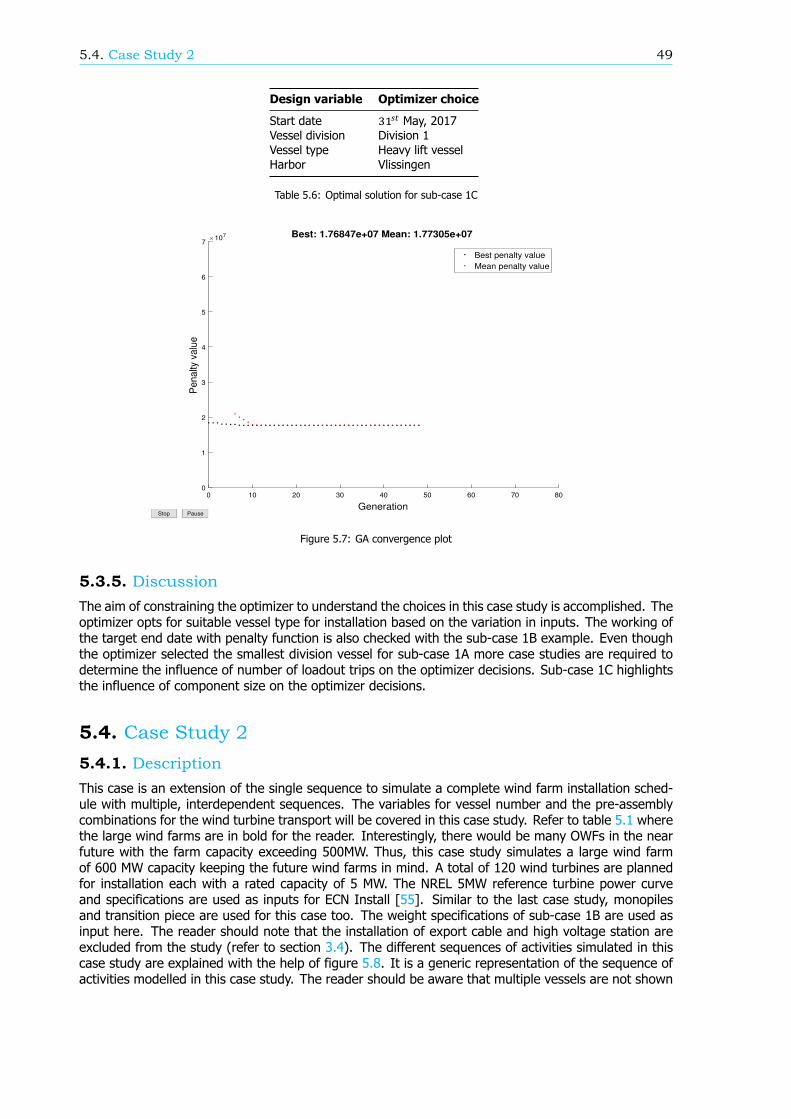
5.4. Case Study 2 49
Design variable Optimizer choice
Start date May, 2017Vessel division Division 1Vessel type Heavy lift vesselHarbor Vlissingen
Table 5.6: Optimal solution for sub-case 1C
0 10 20 30 40 50 60 70 80
Generation
0
1
2
3
4
5
6
7
Penalty
valu
e
107 Best: 1.76847e+07 Mean: 1.77305e+07
Best penalty value
Mean penalty value
PauseStop
Figure 5.7: GA convergence plot
5.3.5. DiscussionThe aim of constraining the optimizer to understand the choices in this case study is accomplished. Theoptimizer opts for suitable vessel type for installation based on the variation in inputs. The working ofthe target end date with penalty function is also checked with the sub-case 1B example. Even thoughthe optimizer selected the smallest division vessel for sub-case 1A more case studies are required todetermine the influence of number of loadout trips on the optimizer decisions. Sub-case 1C highlightsthe influence of component size on the optimizer decisions.
5.4. Case Study 25.4.1. DescriptionThis case is an extension of the single sequence to simulate a complete wind farm installation sched-ule with multiple, interdependent sequences. The variables for vessel number and the pre-assemblycombinations for the wind turbine transport will be covered in this case study. Refer to table 5.1 wherethe large wind farms are in bold for the reader. Interestingly, there would be many OWFs in the nearfuture with the farm capacity exceeding 500MW. Thus, this case study simulates a large wind farmof 600 MW capacity keeping the future wind farms in mind. A total of 120 wind turbines are plannedfor installation each with a rated capacity of 5 MW. The NREL 5MW reference turbine power curveand specifications are used as inputs for ECN Install [55]. Similar to the last case study, monopilesand transition piece are used for this case too. The weight specifications of sub-case 1B are used asinput here. The reader should note that the installation of export cable and high voltage station areexcluded from the study (refer to section 3.4). The different sequences of activities simulated in thiscase study are explained with the help of figure 5.8. It is a generic representation of the sequence ofactivities modelled in this case study. The reader should be aware that multiple vessels are not shown
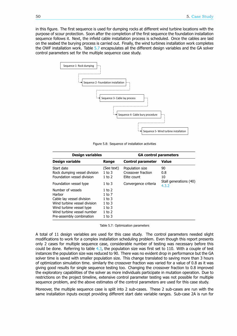
50 5. Case Study
in this figure. The first sequence is used for dumping rocks at different wind turbine locations with thepurpose of scour protection. Soon after the completion of the first sequence the foundation installationsequence follows it. Next, the infield cable installation process is scheduled. Once the cables are laidon the seabed the burying process is carried out. Finally, the wind turbines installation work completesthe OWF installation work. Table 5.7 encapsulates all the different design variables and the GA solvercontrol parameters set for the multiple sequence case study.
Figure 5.8: Sequence of installation activities
Design variables GA control parameters
Design variable Range Control parameter Value
Start date (See text) Population size 90Rock dumping vessel division 1 to 3 Crossover fraction 0.8Foundation vessel division 1 to 2 Elite count 10
Foundation vessel type 1 to 3 Convergence criteriaStall generations (40)4.3.2
Number of vessels 1 to 2Harbor 1 to 7Cable lay vessel division 1 to 3Wind turbine vessel division 1 to 3Wind turbine vessel type 1 to 3Wind turbine vessel number 1 to 2Pre-assembly combination 1 to 3
Table 5.7: Optimization parameters
A total of 11 design variables are used for this case study. The control parameters needed slightmodifications to work for a complex installation scheduling problem. Even though this report presentsonly 2 cases for multiple sequence case, considerable number of testing was necessary before thiscould be done. Referring to table 4.3, the population size was first set to 110. With a couple of testinstances the population size was reduced to 90. There was no evident drop in performance but the GAsolver time is saved with smaller population size. This change translated to saving more than 3 hoursof optimization simulation time. similarly the crossover fraction was varied for a value of 0.8 as it wasgiving good results for single sequence testing too. Changing the crossover fraction to 0.8 improvedthe exploratory capabilities of the solver as more individuals participate in mutation operation. Due torestrictions on the project timeline, extensive control parameter testing was not possible for multiplesequence problem, and the above estimates of the control parameters are used for this case study.
Moreover, the multiple sequence case is split into 2 sub-cases. These 2 sub-cases are run with thesame installation inputs except providing different start date variable ranges. Sub-case 2A is run for
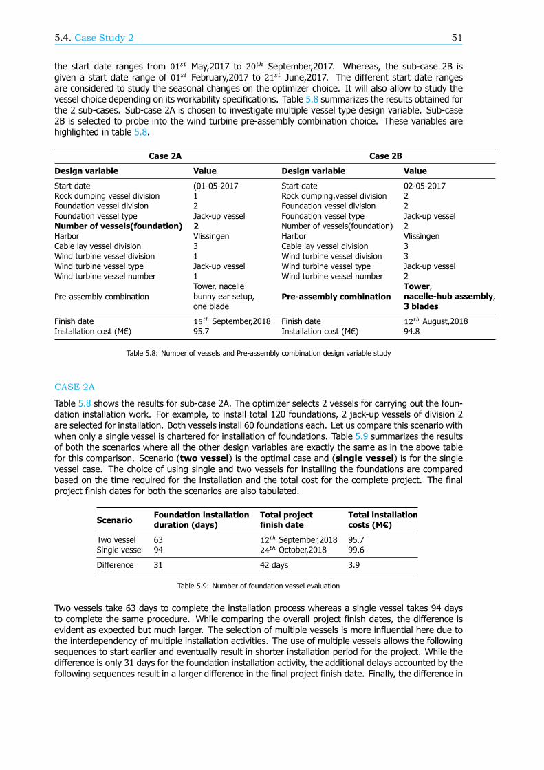
5.4. Case Study 2 51
the start date ranges from 01 May,2017 to 20 September,2017. Whereas, the sub-case 2B isgiven a start date range of 01 February,2017 to 21 June,2017. The different start date rangesare considered to study the seasonal changes on the optimizer choice. It will also allow to study thevessel choice depending on its workability specifications. Table 5.8 summarizes the results obtained forthe 2 sub-cases. Sub-case 2A is chosen to investigate multiple vessel type design variable. Sub-case2B is selected to probe into the wind turbine pre-assembly combination choice. These variables arehighlighted in table 5.8.
Case 2A Case 2B
Design variable Value Design variable Value
Start date (01-05-2017 Start date 02-05-2017Rock dumping vessel division 1 Rock dumping,vessel division 2Foundation vessel division 2 Foundation vessel division 2Foundation vessel type Jack-up vessel Foundation vessel type Jack-up vesselNumber of vessels(foundation) 2 Number of vessels(foundation) 2Harbor Vlissingen Harbor VlissingenCable lay vessel division 3 Cable lay vessel division 3Wind turbine vessel division 1 Wind turbine vessel division 3Wind turbine vessel type Jack-up vessel Wind turbine vessel type Jack-up vesselWind turbine vessel number 1 Wind turbine vessel number 2
Pre-assembly combinationTower, nacellebunny ear setup,one blade
Pre-assembly combinationTower,nacelle-hub assembly,3 blades
Finish date September,2018 Finish date August,2018Installation cost (M€) 95.7 Installation cost (M€) 94.8
Table 5.8: Number of vessels and Pre-assembly combination design variable study
CASE 2A
Table 5.8 shows the results for sub-case 2A. The optimizer selects 2 vessels for carrying out the foun-dation installation work. For example, to install total 120 foundations, 2 jack-up vessels of division 2are selected for installation. Both vessels install 60 foundations each. Let us compare this scenario withwhen only a single vessel is chartered for installation of foundations. Table 5.9 summarizes the resultsof both the scenarios where all the other design variables are exactly the same as in the above tablefor this comparison. Scenario (two vessel) is the optimal case and (single vessel) is for the singlevessel case. The choice of using single and two vessels for installing the foundations are comparedbased on the time required for the installation and the total cost for the complete project. The finalproject finish dates for both the scenarios are also tabulated.
ScenarioFoundation installationduration (days)
Total projectfinish date
Total installationcosts (M€)
Two vessel 63 September,2018 95.7Single vessel 94 October,2018 99.6
Difference 31 42 days 3.9
Table 5.9: Number of foundation vessel evaluation
Two vessels take 63 days to complete the installation process whereas a single vessel takes 94 daysto complete the same procedure. While comparing the overall project finish dates, the difference isevident as expected but much larger. The selection of multiple vessels is more influential here due tothe interdependency of multiple installation activities. The use of multiple vessels allows the followingsequences to start earlier and eventually result in shorter installation period for the project. While thedifference is only 31 days for the foundation installation activity, the additional delays accounted by thefollowing sequences result in a larger difference in the final project finish date. Finally, the difference in
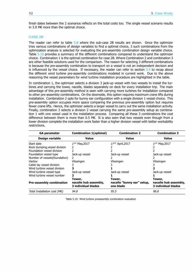
52 5. Case Study
finish dates between the 2 scenarios reflects on the total costs too. The single vessel scenario resultsin 3.9 M€ more than the optimal choice.
CASE 2B
The reader can refer to table 5.8 where the sub-case 2B results are shown. Since the optimizertries various combinations of design variables to find a optimal choice, 3 such combinations from theoptimization analysis is selected for evaluating the pre-assembly combination design variable choice.Table 5.10 provides a summary of the different combinations compared to understand the optimizerchoice. Combination 1 is the optimal combination for case 2B. Where Combination 2 and combination 3are other feasible solutions used for the comparison. The reason for selecting 3 different combinationsis because the pre-assembly combination to transport on a vessel is not an independent decision andis influenced by the vessel choice. If necessary, the reader can refer to section 3.4 to recap aboutthe different wind turbine pre-assembly combinations modeled in current work. Due to the abovereasoning the vessel parameters for wind turbine installation procedure are highlighted in the table.
In combination 1, the optimizer selects a division 3 jack-up vessel with two vessels to install the tur-bines and carrying the tower, nacelle, blades separately on deck for every installation trip. The mainadvantage of this pre-assembly method is seen with carrying more turbines for installation comparedto other pre-assembly combinations. On the downside, this option requires maximum crane lifts duringinstallation. Combination 2 opts for bunny ear configuration with a single division 1 vessel choice. Thispre-assembly option occupies more space comparing the previous pre-assembly option but requiresfewer crane lifts. Hence, the optimizer selects a larger vessel to carry out the same installation activity.Finally, combination 3 selects a division 2 vessel carrying the same pre-assembly setup as combina-tion 1 with one vessel used in the installation process. Comparing all these 3 combinations the costdifference between them is more than 0.5 M€. It is also seen that two vessels even though from alower division complete the installation work faster than a higher division vessel with better workabilityrestrictions.
GA parameter Combination 1(optimal) Combination 2 Combination 3
Design variable Value Value Value
Start date May,2017 April,2017 May,2017Rock dumping,vessel division 2 2 2Foundation vessel division 2 2 2Foundation vessel type Jack-up vessel Jack-up vessel Jack-up vesselNumber of vessels(foundation) 2 2 2Harbor Vlissingen Vlissingen VlissingenCable lay vessel division 3 3 3Wind turbine vessel division 3 1 2Wind turbine vessel type Jack-up vessel Jack-up vessel Jack-up vesselWind turbine vessel number 2 1 1
Pre-assembly combinationTower,nacelle hub assembly,3 individual blades
Tower,nacelle ”bunny ear” setup,one blade
Tower,nacelle hub assembly,3 individual blades
Total Installation cost (M€) 94.8 95.5 96.8
Table 5.10: Wind turbine preassembly combination evaluation

5.4. Case Study 2 53
5.4.2. DiscussionAs seen in table 5.8, 2 sub-cases were run for different start date ranges. The sub-cases presentdifferent design variable combinations and varying installation costs. Sub-case 2A incurs a total of 95.7M€ as project installation expenditure. While sub-case 2B results in a lower cost of 94.8 M€. Theoptimizer chooses the division 3 cable lay vessel for both sub-cases. This is accounted due to the lowchartering cost for the vessel in this division. As a drawback, the division 3 cable vessel needs 2 trips torefill with new cable and finish the laying procedure. Even if a larger division vessel is used for layingprocess, the installation cost is at least 0.3 M€ higher compared to the optimal choice of division 3vessel. Similarly, case study 2 highlights an interesting aspect about the choice of vessel type for theinstallation of foundations and wind turbines. For both the case 2A and case 2B Jack-up vessel typeare the best choice for the installation work. It authenticates the popularity of jack-up vessel typesin the OWF installation industry due to their purpose built functionality and superior workability whencompared to jack-up barges and heavy lift vessel types in current study.
Referring to table 5.9 the different start dates design variable tried by the optimizer while all the othervariables remaining same from the table. Figure 5.9 represents the trend observed with installationcosts incurred for different start dates. The installation costs are average of 100 different realizationsfor every start date variable choice. It is seen that when the start date range is set from Februaryto July (sub-case 2B) the optimal choice for the start date is in May. The plot shows the reduction incost as it moves closer to May and then increases again. When the start date range is set from Mayto September (sub-case 2A) the optimizer again selects the best start date in May. With a delayedstart in the sub-case 2A, the project cost continues with an increasing trend. The trends seen in boththe cases are slightly different. In case 2A, all the start dates before 20 August have a increasinginstallation cost due to weather influencing the delays in the project. The start dates after 20 Augustare a combination of the weather affecting the project costs with the penalty value also added due toexceeding the set target date for the project. In case 2B, the start dates in February and July resultin high installation cost only due to the weather delays and not because of penalty function. Thereader should note that while the optimizer finds similar start dates for both the sub-cases, the optimalcombination of the design variables and weather realizations are different in both sub-cases. Thus, thetotal installation costs obtained are also different for the sub-case 2A and 2B.
Let us refer to the figure 5.8 where the different sequences for this case study with their interdepen-dencies are shown. Starting in the month of may for both the cases 2A and 2B result in the cableburying process falling in the winter season of 2017 to 2018. The burying process uses a ROV anda multi-purpose vessel for the installation procedure (refer to section 3.4). The hiring cost for theseresources are relatively cheap when compared to other installation vessels in the project. Even thoughthe delays encountered during cable burying process is high, the total influence on the project instal-lation cost is acceptable. Hence, it results in the least installation costs when starting in May. Thisdiscussion also highlights the influence interdependancy can have on multiple sequence projects. Thestart date plot (fig. 5.9) emphasizes the importance of start date variable and its influence on all otherdesign variables in the study.
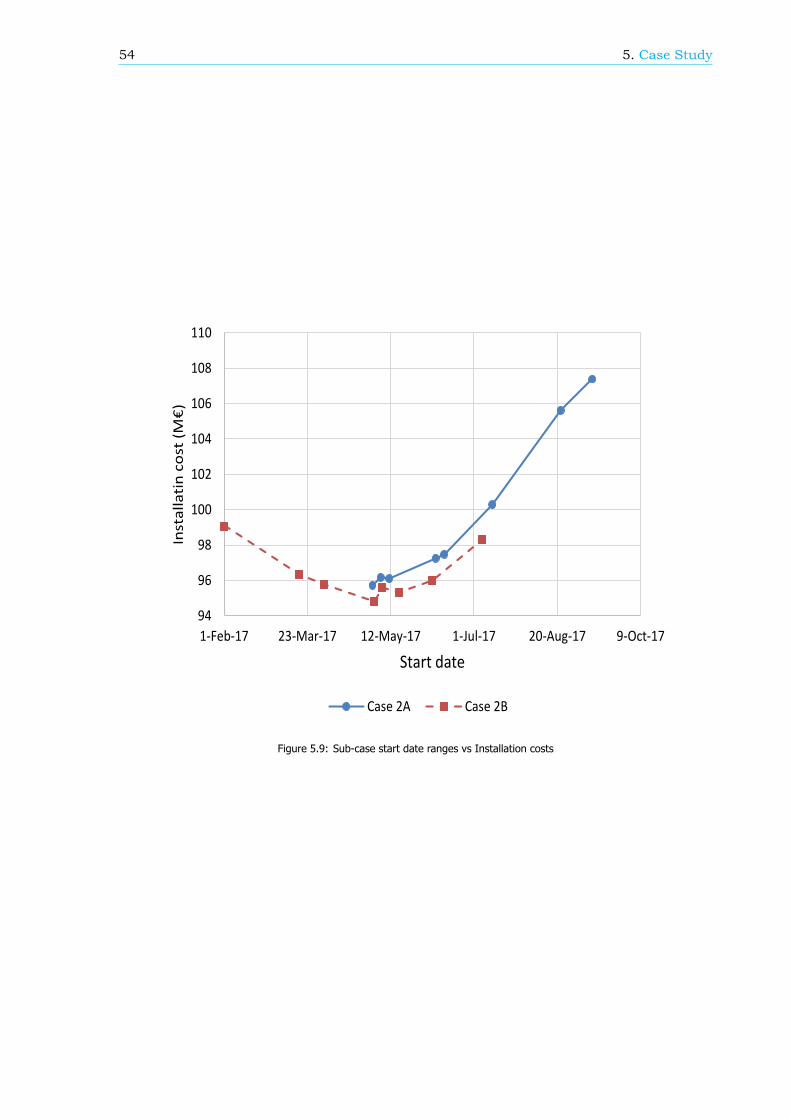
54 5. Case Study
Figure 5.9: Sub-case start date ranges vs Installation costs
6Conclusions and Future Work
This chapter summarizes the learnings from this thesis study and gives some recommendations forfuture work.
6.1. ConclusionsThe objective of the study was the development of an approach to obtain minimized cost for OWFinstallation procedure while having a target end date of significance. Consequently, the primary focusof the project was to provide flexibility in modeling OWF installation schedules and delivering optimalsolutions in affordable computation times. The new approach developed with ECN shows promisingresults for optimizing OWF installation logistics with a target date set by the decision maker.
A concise literature review demonstrated the significance of the current research and the potential thatmetaheuristic approaches bring to solve installation scheduling problems. The genetic algorithm waschosen as the optimization procedure to use for this study. The objective of the optimization processall throughout this research was the minimization of installation costs. The target end date for anygiven project is implemented in the form of a constraint to steer the solution within the specified limit.The installation of wind turbines offshore in harsh weather conditions inexorably introduces a certainlevel of uncertainty in the project schedule. To better account for this uncertainty due to weather, asynthetic weather data simulator was provided by ECN for this research. The modular structure of GAin MATLAB toolbox allowed efficient customization to create the new architecture with ECN Install. Thedecision to use the Integer GA solver was favorable for the current study, which is supported by thecase study results.
Furthermore, a significant part of the current work involved the building of a new architecture forrunning the optimization analysis with ECN Install. The novel approach required the addition of newblocks for Automated Planning (AP), Uncertainty Consideration (UC), and Constraint Evaluation (CE) tointegrate the optimizer with ECN Install efficiently (refer to figure 2.2). The new approach obligated theneed for blocks mentioned above in accomplishing the thesis objective. The AP block was constructedto prepare the installation planning based on the design variable combinations fed by the optimizerand eventually run this planning in ECN Install. Efforts were made to provide the possibility of housinga range of installation sequences, but, the limitation of working with pre-defined planning templateswas inevitable. Nonetheless, profound care was taken while building these templates for differentinstallation activities, since mistakes in the template would result in wrong optimization choices. Thus,all the templates were created based on research about the actual installation procedures employedin the offshore wind industry. Overlooking the limitations of the AP block, the approach worked wellwith GA optimization procedure to generate new planning for every individual combination of decisionvariables in quick times (few seconds). The AP block approach has shown promising results for futuredevelopments.
55
56 6. Conclusions and Future Work
A UC block is provided to account for the variability in weather while interpreting the total installationcosts. A compact investigation on studying the uncertainty due to weather in a project allowed tofix the final choice of simulating 100 different weather instances for every new planning generatedduring the optimization process. The choice of running a large number of weather realizations wasreasonable to determine a more accurate mean for installation costs. However, the 100 unique resultsshow a considerable number of simulations having installation costs higher than the mean value usedfor the optimization procedure. Though initially planned to incorporate the uncertainty variable in theform of a probabilistic constraint was not successful in this study with the GA solver, it is suggested toexplore this approach for better quantifying the uncertainty in OWF installation projects.
The CE block is modeled to accommodate the target end date exceedance check. The CE block functionswith the UC block to penalize any project scenario exceeding the target date set by the user. To thebest of authors knowledge, there is no research in the literature on optimization of OWF installationlogistics with a target end date requirement. The case studies reflect the importance of setting anappropriate target date and the influence of the penalty value on the total installation costs.
Furthermore, the current versions of ECN Install were only able to simulate installation planning withmultiple sequences independent of each other. For this reason, a new method is developed to in-corporate interdependency between the various installation sequences for the installation schedulingproblem. This allowed a realistic evaluation of multiple sequence project in the new optimization pro-cedure where the end date of the first installation sequence would impact the start of the followingsequence. With the support of literature, the main control parameters affecting the performance ofthe GA were identified. These parameters include population size, elite count, and crossover fraction.A pragmatic approach is followed towards modeling an abstract problem for the GA control param-eter tuning process. This was mainly preferred, as the abstract problem allowed quick evaluationsand provided the possibility to study the parameter variations more extensively. This study shows therequirement for tuning the control parameters specific to the problem studied with the GA solver andrecommends carrying out the testing with simple problems to obtain quick solutions. Consequently,the knapsack problem results pinpointed the same reality in this thesis.
Different categories of design variables were employed in this study. These include the start date, vesseldivision, vessel type, vessel number, harbor and pre-assembly combinations of the wind turbine duringload-out. When evaluating all the different design variables, the start date was the most influentialin this study. The variation in start date resulted in different combinations of other remaining designvariables. In the current analysis of the installation logistics, the choice of the port was not a usefuldesign variable, since in the optimization procedure it always resulted in the nearest selection. Thechoice of port might become less straightforward, and therefore a more interesting to study as a designvariable when onshore logistics parameters are also included in the optimization procedure.
To summarize, the key result of this research to provide an approach to obtain the minimized costs fora given OWF installation strategy with a target date is efficiently achieved. Furthermore, the differentcase study results show the prospects of incorporating optimization procedure in OWF installationscheduling problems. Finally, even though the study focused on the optimization procedure, specificwind farm inputs could help evaluate the optimizer performance better and improve the model further.
6.2. Future workThe use of a metaheuristic optimization method in this project was unavoidable with the high levelof complexity in installation scheduling problems. Even though the GA performed adequately for thecurrent study, the overall analysis times are long and would increase with the addition of new designvariables. It could be interesting to explore other metaheuristic methods like the PSO or ABC algorithmsfor solving OWF installation strategies.
This study focuses on a single objective to minimize the total installation cost for a project. It would beworthwhile to scale the problem to a multi-objective case where both cost and duration are optimized.Additionally, a significant improvement area is seen with the AP block implementation procedure. Whilethe method is sufficient to function with the current versions of ECN Install, with more complex se-quence interdependencies introduced in the future versions the AP block implementation will need

6.2. Future work 57
improvements. Also, the AP block work with pre-defined templates for constructing different instal-lation sequences. This limitation can be removed by making more standardized activity blocks liketravel, loading and installation blocks based on the type of installation. This can add more flexibilitywhile creating schedules with AP block.
Likewise, the optimization approach implemented in this study assumes 100% availability of a particularvessel type, port or equipment while running the simulation. Populating the different vessel, port,and equipment libraries with actual resource data with availability information could result in diversesolutions. Also, the implementation of penalty function for the target end date can be explored moreextensively to understand its influence on the optimizer choices.
Moreover, an area which could be further researched is the uncertainty quantification of weather foroptimization study in installation logistics. Hence, a complete distribution of results could be used tofind the optimal choice of design variables. Finally, extensive GA control parameter tuning could not beconducted for multiple sequence projects in this dissertation and it will certainly be beneficial to find theoptimal values for interdependent sequences to obtain the best performance with genetic algorithm.

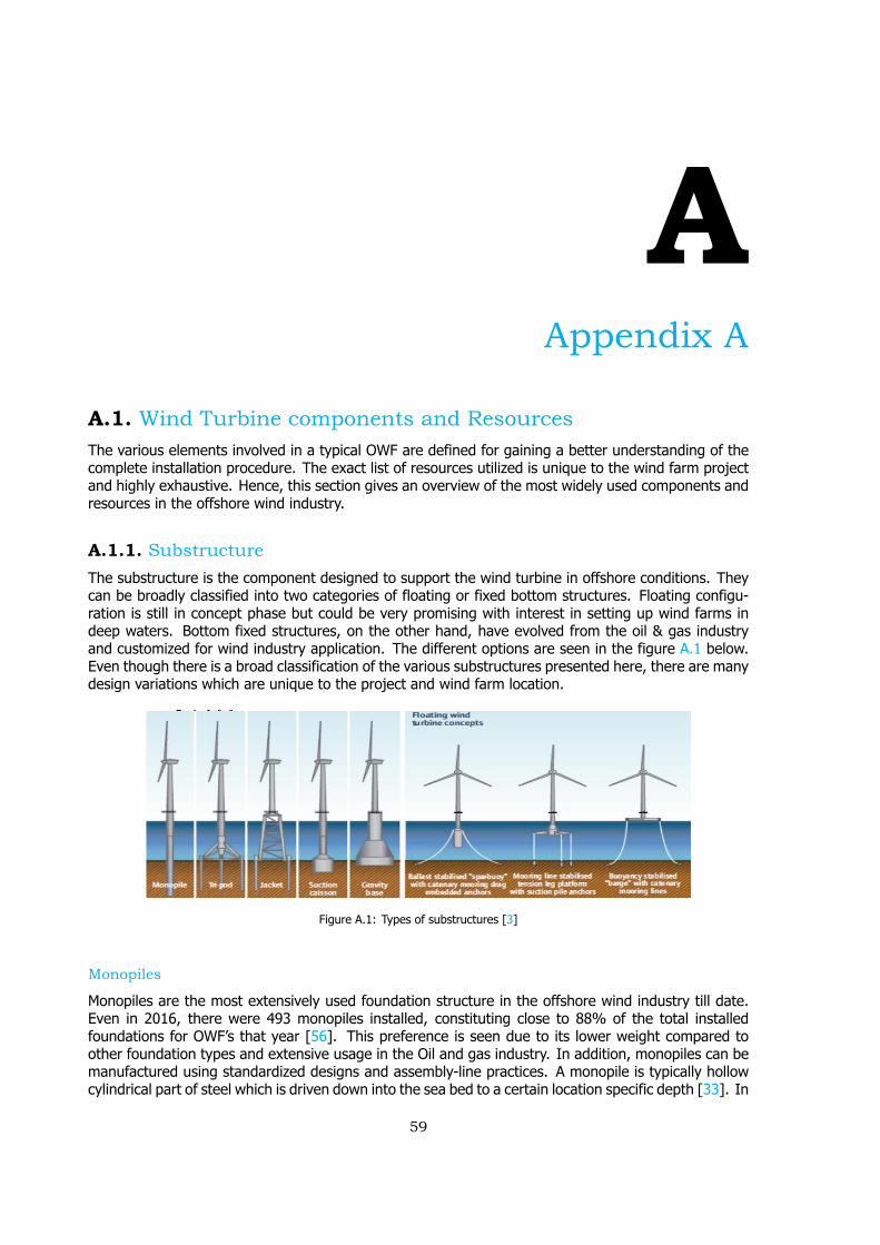
AAppendix A
A.1. Wind Turbine components and ResourcesThe various elements involved in a typical OWF are defined for gaining a better understanding of thecomplete installation procedure. The exact list of resources utilized is unique to the wind farm projectand highly exhaustive. Hence, this section gives an overview of the most widely used components andresources in the offshore wind industry.
A.1.1. SubstructureThe substructure is the component designed to support the wind turbine in offshore conditions. Theycan be broadly classified into two categories of floating or fixed bottom structures. Floating configu-ration is still in concept phase but could be very promising with interest in setting up wind farms indeep waters. Bottom fixed structures, on the other hand, have evolved from the oil & gas industryand customized for wind industry application. The different options are seen in the figure A.1 below.Even though there is a broad classification of the various substructures presented here, there are manydesign variations which are unique to the project and wind farm location.
Figure A.1: Types of substructures [3]
Monopiles
Monopiles are the most extensively used foundation structure in the offshore wind industry till date.Even in 2016, there were 493 monopiles installed, constituting close to 88% of the total installedfoundations for OWF’s that year [56]. This preference is seen due to its lower weight compared toother foundation types and extensive usage in the Oil and gas industry. In addition, monopiles can bemanufactured using standardized designs and assembly-line practices. A monopile is typically hollowcylindrical part of steel which is driven down into the sea bed to a certain location specific depth [33]. In
59

60 A. Appendix A
most cases, there is an additional element used to link the turbine tower with the monopile structure.This component is called the transition piece. It also acts as a landing base for the technicians toaccess the turbine. To ensure the verticality of the wind turbine and account for the slight degreeof inclination after pile driving operation, there is a special cement called Grout applied between themonopile and the transition piece[57]. While grout connections are considered as industry regular,number of connections have failed, preceding to slippage and improper stresses in structures. Thus,new methods like bolting and slip joints are becoming popular with new installations[58].
Scour Protection
Scour is a type of erosion of soil around the structure in the sea bed. This is especially significant inlocations with tidal currents around the structure. Based on experience, it is stated that the scour holecan reach around 1.5 times the pile diameter [29]. In such cases, it becomes beneficial to prepare arock bed around the structure to avoid the above scenario. Scour protection is applied to foundationswhich are secured to the sea bed, seen in the figureA.1.
Jackets
These type of structures are increasingly becoming popular for deep waters where monopiles are noteconomical. Jackets are massive steel lattice tower with triangulated structures providing strength andrequired stability. Jackets are installed by fixing them to the sea bed with three or four pin-piles whichare similar to smaller versions of monopiles. The steel needed to build jackets is less compared tomonopiles in most cases; hence there is some material cost saving. The major drawback is seen to bethe precise welding required for such large structures to resist long term wind and wave loads[59].
Gravity Based Structure
Gravity based structures are concrete conical shape foundations with a flat base to place on the seabed. They are typically secured with ballast to prevent against scour protection. They are a popularchoice of foundation for shallow waters or tough sea beds where pilling is hard [60].
Floating Structures
These structures are a viable option when the water depths are more than 40m. Typically the turbineis secured on a floating mass in the sea which could be a single cylindrical buoy or a semi-submersibleplatform. A significant advantage is seen in the installation phase where a complete turbine can beassembled onshore and installed in no time at the farm location saving both time and costs. On thecontrary, the floating structure needs to remain straight at all times and withstand the harsh wind andwave conditions. There is substantial research being invested into floating structures which might havewide spread effects in the complete value chain [61].
A.1.2. Wind Turbine Components
The offshore wind turbines are very similar to the onshore machines used in the industry, with certainmodifications to design to handle the offshore conditions. Size and noise regulations do not limit theoffshore turbines compared to onshore turbines; hence much larger turbines are preferred to reducethe overall project costs. The average capacity of offshore turbines ranges around 5 MW where it isjust about 2 MW for onshore application. Currently, 10 MW turbines are under testing for offshoreapplication [62]. A typical horizontal axis wind turbine consists of various separate components whichrequire being assembled before going into operation. The figure below shows these components forbetter understanding. There are multiple installation procedure followed in the industry are discussedin chapter 3.
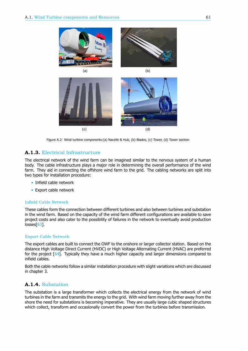
A.1. Wind Turbine components and Resources 61
Figure A.2: Wind turbine components:(a) Nacelle & Hub, (b) Blades, (c) Tower, (d) Tower section
A.1.3. Electrical InfrastructureThe electrical network of the wind farm can be imagined similar to the nervous system of a humanbody. The cable infrastructure plays a major role in determining the overall performance of the windfarm. They aid in connecting the offshore wind farm to the grid. The cabling networks are split intotwo types for installation procedure:
• Infield cable network
• Export cable network
Infield Cable Network
These cables form the connection between different turbines and also between turbines and substationin the wind farm. Based on the capacity of the wind farm different configurations are available to saveproject costs and also cater to the possibility of failures in the network to eventually avoid productionlosses[63].
Export Cable Network
The export cables are built to connect the OWF to the onshore or larger collector station. Based on thedistance High Voltage Direct Current (HVDC) or High Voltage Alternating Current (HVAC) are preferredfor the project [64]. Typically they have a much higher capacity and larger dimensions compared toinfield cables.
Both the cable networks follow a similar installation procedure with slight variations which are discussedin chapter 3.
A.1.4. SubstationThe substation is a large transformer which collects the electrical energy from the network of windturbines in the farm and transmits the energy to the grid. With wind farm moving further away from theshore the need for substations is becoming imperative. They are usually large cubic shaped structureswhich collect, transform and occasionally convert the power from the turbines before transmission.

62 A. Appendix A
Figure A.3: Electrical infrastructure
Figure A.4: Offshore substation
A.1.5. VesselsVessels are the most cost incurring component in the wind farm installation procedure. Over the pasttwo decades of learning in the offshore wind industry the vessels have come a long way and have beenpurpose built for the required operations. Most vessels involved in the installation phase are expensiveto charter and demand efficient planning to keep the overall installation costs in check. Some popularvessels used in the OWF installation process are shown below.
The most popular installation vessels used for foundations and turbines are the jack-up vessel cate-gories. Next, closely followed by the heavy lift and Floating Sheerleg Crane types. The figureA.6(c)shows a Floating sheerleg crane installing a jacket at sea. Similarly, pictures of jack-up vessels areshown in figureA.7(b). The differences between the different vessels are discussed in chapter 3 basedon the type of installation applied during the project build.
A.1.6. Equipment
The installation of large components requires purpose built equipment to assist in the assembly process.Most equipment used have been adopted from different industries to aid the installation of Wind Tur-bines offshore. The following sections summarize some of the most popularly used types of equipmentduring the installation phase.
Cranes
Cranes are essential equipment part of the installation vessels in the market. They are used to lift theheavy and large wind farm components required to be installed. Few important parameters like liftcapacity, radius and boom length play a major role in deciding the vessel capability for the necessaryinstallation activity [15].
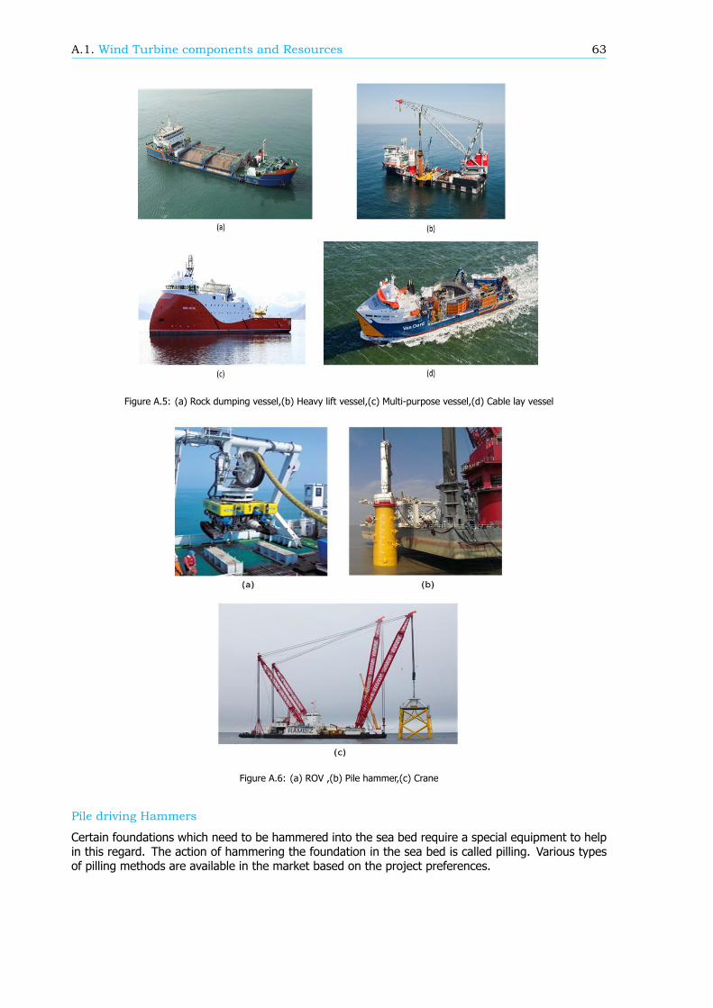
A.1. Wind Turbine components and Resources 63
Figure A.5: (a) Rock dumping vessel,(b) Heavy lift vessel,(c) Multi-purpose vessel,(d) Cable lay vessel
Figure A.6: (a) ROV ,(b) Pile hammer,(c) Crane
Pile driving Hammers
Certain foundations which need to be hammered into the sea bed require a special equipment to helpin this regard. The action of hammering the foundation in the sea bed is called pilling. Various typesof pilling methods are available in the market based on the project preferences.
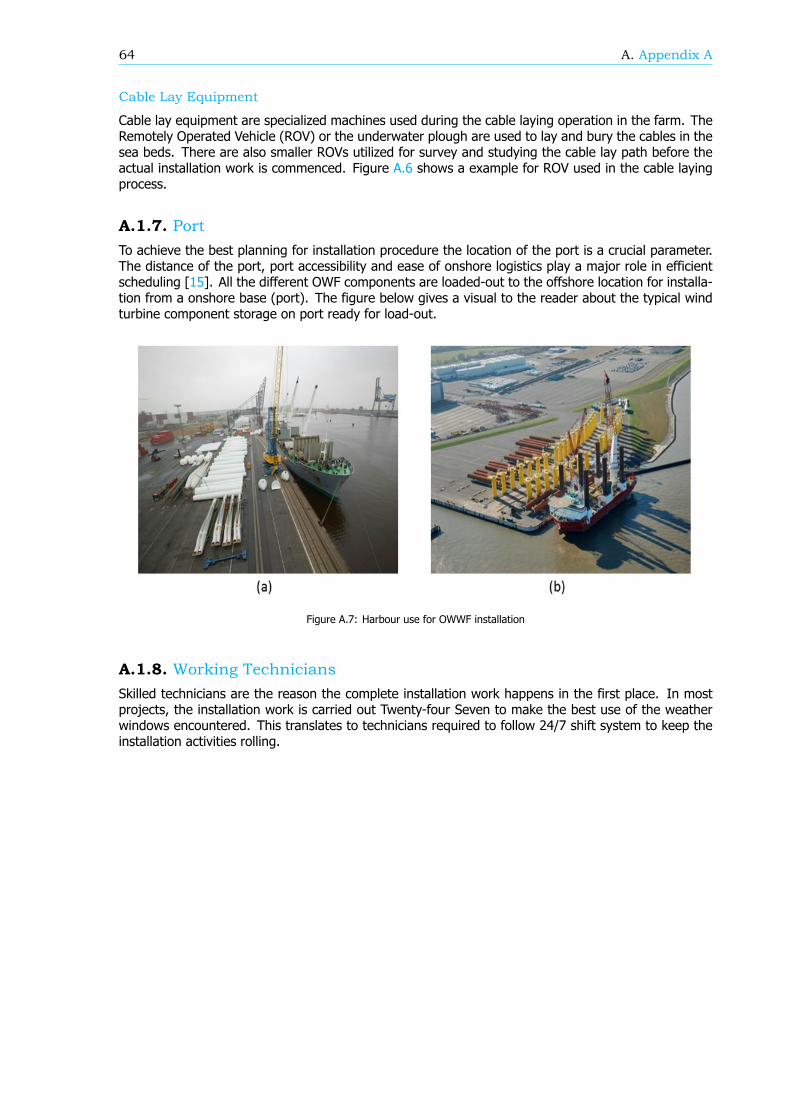
64 A. Appendix A
Cable Lay Equipment
Cable lay equipment are specialized machines used during the cable laying operation in the farm. TheRemotely Operated Vehicle (ROV) or the underwater plough are used to lay and bury the cables in thesea beds. There are also smaller ROVs utilized for survey and studying the cable lay path before theactual installation work is commenced. Figure A.6 shows a example for ROV used in the cable layingprocess.
A.1.7. PortTo achieve the best planning for installation procedure the location of the port is a crucial parameter.The distance of the port, port accessibility and ease of onshore logistics play a major role in efficientscheduling [15]. All the different OWF components are loaded-out to the offshore location for installa-tion from a onshore base (port). The figure below gives a visual to the reader about the typical windturbine component storage on port ready for load-out.
Figure A.7: Harbour use for OWWF installation
A.1.8. Working TechniciansSkilled technicians are the reason the complete installation work happens in the first place. In mostprojects, the installation work is carried out Twenty-four Seven to make the best use of the weatherwindows encountered. This translates to technicians required to follow 24/7 shift system to keep theinstallation activities rolling.

BAppendix B
B.0.1. Inputs and Planning
Inputs and planning module is primarily a setup block for the installation schedule. The basic parame-ters necessary for the complete planning process are stored in this section. The table below summarizesthe inputs taken by ECN INSTALL tool.
Sub-module Parameter
Wind Turbine Turbine type, Rater power, Hub height, Number of turbines, Power curve
MetOcean Data Weather data file, Resolution
Operational Bases Port name, Distance to farm, Cost information
Components Component names, Weight specifications
Equipment Equipment cost and duration data
Vessels Specific vessel cost and duration details
Working shifts Different shift split-up details
Costs Project management and fixed project costs
Table B.1: ECN Install Input parameters
The complexity and accuracy of the planning depend on the inputs provided as shown in the tableabove. This module is necessary for generating a planning for the desired installation procedure.Before moving to next section, this is a good time to define few relevant terms which will frequentlybe used in the report. The offshore wind farm installation procedure in highly repetitive and allows foriterating the repeating activities once they are defined initially. The planning process in the INSTALLtool is classified under STEP, GROUP and SEQUENCE levels to represent the same. The Sequenceis the first level in the installation planning. This level defines the significant installation activities tobe carried out multiple times in a wind farm. For example, the installation of support structures orcable installation for OWF is classified under sequence level. Next is the Group level which is housedinside the larger Sequence levels. It encapsulates the sub-activities that take place in a Sequence. Anexample of this level is the loading of sub-structures on a particular vessel selected for installation inSequence. Installation of cable between two turbine locations is another example. Finally, the smallestblock of the planning is the Step level. These levels store the actual operation taking place in thegroup levels. The piling of a monopile is an example of Step level activity. The different levels can bevisualized by referring to the figure B.1.
65
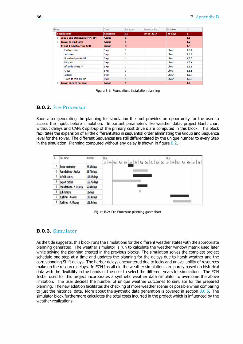
66 B. Appendix B
Figure B.1: Foundations installation planning
B.0.2. Pre-Processor
Soon after generating the planning for simulation the tool provides an opportunity for the user toaccess the inputs before simulation. Important parameters like weather data, project Gantt chartwithout delays and CAPEX split-up of the primary cost drivers are computed in this block. This blockfacilitates the expansion of all the different step in sequential order eliminating the Group and Sequencelevel for the solver. The different Sequences are still differentiated by the unique number to every Stepin the simulation. Planning computed without any delay is shown in figure B.2.
Figure B.2: Pre-Processor planning gantt chart
B.0.3. Simulator
As the title suggests, this block runs the simulations for the different weather states with the appropriateplanning generated. The weather simulator is run to calculate the weather window matrix used laterwhile solving the planning created in the previous blocks. The simulation solves the complete projectschedule one step at a time and updates the planning for the delays due to harsh weather and thecorresponding Shift delays. The harbor delays encountered due to locks and unavailability of resourcesmake up the resource delays. In ECN Install old the weather simulations are purely based on historicaldata with the flexibility in the hands of the user to select the different years for simulations. The ECNInstall used for this project incorporates a synthetic weather data simulator to overcome the abovelimitation. The user decides the number of unique weather outcomes to simulate for the preparedplanning. The new addition facilitates the checking of more weather scenarios possible when comparingto just the historical data. More about the synthetic data generation is covered in section B.0.5. Thesimulator block furthermore calculates the total costs incurred in the project which is influenced by theweather realizations.

67
B.0.4. Post-ProcessorOnce the simulations are completed, the different results are post-processed and output to a readableformat for the user is generated. The tool provides the option of exporting all the results to MS Excel,final planning to MS Project Gantt chart and saves various graphs to better visualize the results. Thefigure B.3 B.4 shows an example gantt chart post simulation and a pie chart for delays.
Figure B.3: Post-Process gantt chart
Figure B.4: Average delays breakdown per step and delay type.
B.0.5. Install ModelA short description of how the installation modeling is carried out in the tool is vital for the reader to getfamiliar with the calculation logic applied in the backend code. This forms the footing to understandthe integration of optimization approach for the tool in the later chapters. Soon after the planning iscreated all the installation activities are expanded into steps for the simulation to proceed. Currently, themeteorological parameters for wind speed (Ws) and significant wave height (Hs) are taken into accountin the tool. In numerous situations, a step could have various restrictions based on the resources underconsideration. In the end, one specific weather restriction for each step is assigned from evaluatingthe minimum restrictions of all the resources in play. By applying the above condition for every step,all the particular restrictions are valued.
Usually, the weather window selected for installation activity is slightly larger than the step duration toaccount for uncertainty. The model makes sure the required weather window is available before thestep is executed. The different delays are accounted at each step and added to the predefined stepduration.
It is important to mention that the Steps are categorized into three types. The Loading step wherethe specific component is loaded onto the vessel at the port. Next, the traveling step for any transit

68 B. Appendix B
of vessel between the harbor and wind farm. Finally, the Installation step which describes all theinstallation activities that take place in the project using the vessel and equipment. Depending on theuser selection for every step specific options are enabled. Likewise, the model also demands the inputinformation about the shifts used in the project. Where the loading and installation step types areclassified as a shift-splittable category, which means that one technician’s shift can start the step anda different one could complete it. Whereas in the case of traveling step type the shift is considered asnon-splittable. It implies that if the step duration is more than the maximum shift duration the step isnot performed, and an error is displayed. The above process is carried out starting from the first stepto the last one for the planning created by the user.
While the ECN Install old, worked with only historical weather data the ECN Install used for this thesisincorporates a synthetic weather data generator. It is important to understand more about the weathersimulator as it plays a significant role in the optimization process. As mentioned in the introductionchapter installation activities for OWFs involve uncertainty due to weather conditions. Meaning, windand wave conditions are stochastic events and inherently random. Historical data is capable of capturingonly part of this irregularity in the time series. Hence, if an only small number of weather data areused for the evaluations, it would result in the creation of prejudice in the output results. To overcomethe limitations, a new stochastic weather simulator is developed in-house to run a large number ofindependent time-domain simulations for any project the decision maker intends to evaluate. Thereader can acquire more details about the actual procedure followed to create this weather simulatorby referring to report by C.F.W. Stock-Williams [65]. To conclude, the weather simulator integrated withECN Install trains on the time series data provided by the user and generates the synthetic weatherrealizations stating from the project start year till five years ahead of the start year.
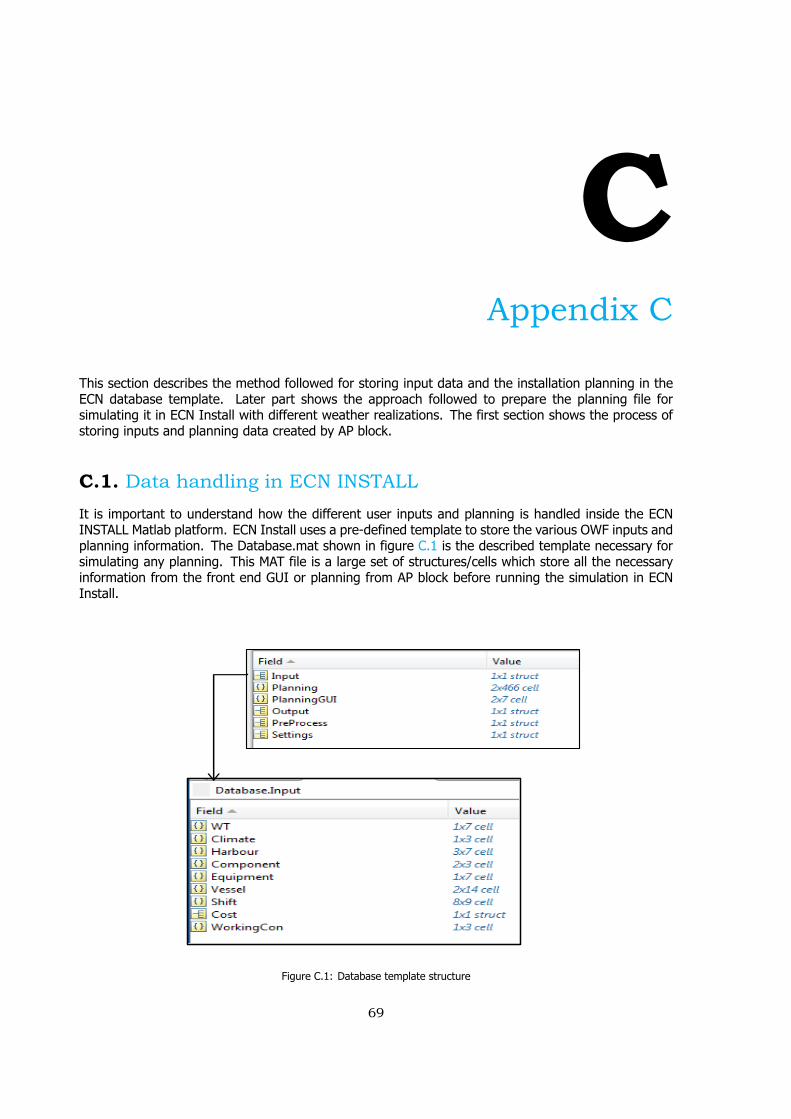
CAppendix C
This section describes the method followed for storing input data and the installation planning in theECN database template. Later part shows the approach followed to prepare the planning file forsimulating it in ECN Install with different weather realizations. The first section shows the process ofstoring inputs and planning data created by AP block.
C.1. Data handling in ECN INSTALLIt is important to understand how the different user inputs and planning is handled inside the ECNINSTALL Matlab platform. ECN Install uses a pre-defined template to store the various OWF inputs andplanning information. The Database.mat shown in figure C.1 is the described template necessary forsimulating any planning. This MAT file is a large set of structures/cells which store all the necessaryinformation from the front end GUI or planning from AP block before running the simulation in ECNInstall.
Figure C.1: Database template structure
69
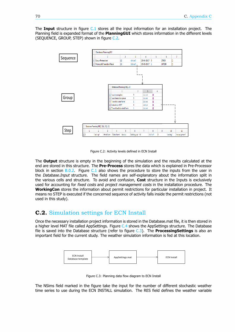
70 C. Appendix C
The Input structure in figure C.1 stores all the input information for an installation project. ThePlanning field is expanded format of the PlanningGUI which stores information in the different levels(SEQUENCE, GROUP, STEP) shown in figure C.2.
Figure C.2: Activity levels defined in ECN Install
The Output structure is empty in the beginning of the simulation and the results calculated at theend are stored in this structure. The Pre-Process stores the data which is explained in Pre-Processorblock in section B.0.2. Figure C.1 also shows the procedure to store the inputs from the user inthe Database.Input structure. The field names are self-explanatory about the information split inthe various cells and structure. To avoid and confusion, Cost structure in the Inputs is exclusivelyused for accounting for fixed costs and project management costs in the installation procedure. TheWorkingCon stores the information about permit restrictions for particular installation in project. Itmeans no STEP is executed if the concerned sequence of activity falls inside the permit restrictions (notused in this study).
C.2. Simulation settings for ECN InstallOnce the necessary installation project information is stored in the Database.mat file, it is then stored ina higher level MAT file called AppSettings. Figure C.4 shows the AppSettings structure. The Databasefile is saved into the Database structure (refer to figure C.3). The ProcessingSettings is also animportant field for the current study. The weather simulation information is fed at this location.
Figure C.3: Planning data flow diagram to ECN Install
The NSims field marked in the figure take the input for the number of different stochastic weathertime series to use during the ECN INSTALL simulation. The RES field defines the weather variable
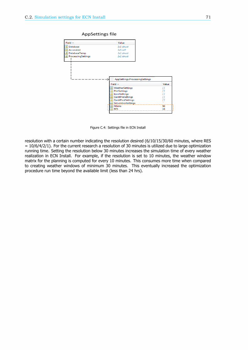
C.2. Simulation settings for ECN Install 71
Figure C.4: Settings file in ECN Install
resolution with a certain number indicating the resolution desired (6/10/15/30/60 minutes, where RES= 10/6/4/2/1). For the current research a resolution of 30 minutes is utilized due to large optimizationrunning time. Setting the resolution below 30 minutes increases the simulation time of every weatherrealization in ECN Install. For example, if the resolution is set to 10 minutes, the weather windowmatrix for the planning is computed for every 10 minutes. This consumes more time when comparedto creating weather windows of minimum 30 minutes. This eventually increased the optimizationprocedure run time beyond the available limit (less than 24 hrs).

Bibliography
[1] Global wind energy council, (), accessed: 2017-08-20.
[2] The Power to Change: Solar and Wind Cost Reduction Potential to 2025, Tech. Rep. (InternationalRenewable Energy Agency(IRENA), 2016).
[3] M. J. Kaiser and B. Snyder, Offshore wind energy cost modeling: installation and decommissioning,Vol. 85 (Springer Science & Business Media, 2012).
[4] MATLAB, Global Optimization Toolbox, Tech. Rep. (MathWorks,Inc, 2017).
[5] Borssele Wind Farm Zone, project and site description, Tech. Rep. (Netherlands EnterpriseAgency(RVO.nl), August 2015).
[6] Offshore wind farm database, Accessed: 2017-10-12.
[7] Paris climate change agreement, Accessed: 2017-04-10.
[8] Global wind energy council, (), accessed: 2017-06-25.
[9] Offshore wind - Global wind 2015 report, Tech. Rep. (Global wind energy council, 2016).
[10] Global offshore wind installation by 2020, Accessed: 2017-09-28.
[11] European commission, climate action, Accessed: 2017-04-15.
[12] B. Scholz-Reiter, H. Karimi, M. Lütjen, J. Heger, and A. Schweizer, Towards a heuristic for schedul-ing offshore installation processes, in Proceedings of the 24th International Congress on ConditionMonitoring (COMADEM) (2011) pp. 999–1008.
[13] Roland berger sees europe offshore wind at 40 gw by 2020, Accessed: 2017-08-16.
[14] Flow cost model, (2017).
[15] E. Uraz, Offshore Wind Turbine Transportation and Installation Analyses, M.eng. thesis, GotlandUniversity (2011).
[16] E. Rosenauer, Investment costs of offshore wind turbines, Tech. Rep. CSS14-27 (Center for Sus-tainable Systems, 2014).
[17] B. Scholz-Reiter, J. Heger, M. Lütjen, and A. Schweizer, Amilp for installation scheduling of offshorewind farms, International Journal Of Mathematical Models And Methods In Applied Sciences 5,371 (2010).
[18] M. Lütjen, H. R. Karimi, et al., Approach of a port inventory control system for the offshoreinstallation of wind turbines, in The Twenty-second International Offshore and Polar EngineeringConference (International Society of Offshore and Polar Engineers, 2012).
[19] A. Ait-Alla, M. Quandt, and M. Lutjen, Aggregate installation planning of offshore wind farms, inProceedings of the 7th international conference on communications and information technology(CIT 13). Cambridge (US) (2013) pp. 130–35.
[20] Y. T. Muhabie, J.-D. Caprace, C. Petcu, and P. Rigo, Improving the installation of offshore windfarms by the use of discrete event simulation, Improving the Installation of Offshore Wind Farmsby the use of Discrete Event Simulation (2015).
[21] C. A. Irawan, D. Jones, and D. Ouelhadj, Bi-objective optimisation model for installation schedul-ing in offshore wind farms, Computers & Operations Research 78, 393 (2017).
73
74 Bibliography
[22] P. Collet and J.-P. Rennard, Stochastic optimization algorithms, arXiv preprint arXiv:0704.3780(2007).
[23] S. Luke, Essentials of metaheuristics, Vol. 113 (Lulu Raleigh, 2009).
[24] Particle swarm optimization, Accessed: 2017-07-14.
[25] Genetic algorithm optimization, Accessed: 2017-07-14.
[26] I. F. Vis and E. Ursavas, Assessment approaches to logistics for offshore wind energy installation,Sustainable energy technologies and assessments 14, 80 (2016).
[27] Great circle distance, (), accessed: 2017-06-15.
[28] 4c offshore port database, (), accessed: 2017-06-14.
[29] M. Zaaijer and J. Van der Tempel, Scour protection: a necessity or a waste of money, in Proceed-ings of the 43 IEA Topixal Expert Meeting (2004) pp. 43–51.
[30] Gemini windpark installation animation, Accessed: 2017-08-10.
[31] M. Conconi and G. Corbetta, WP Framework/ Industry Challenges Report- supply chain and logis-tics, Tech. Rep. (EWEA,GDG,A2SEA, 2014).
[32] Floating monopiles to owf location, Accessed: 2017-08-10.
[33] Monopiles support structures, Accessed: 2017-08-14.
[34] Cable Burial Risk Assessment Methodology: Guidance for the Preparation of Cable Burial Depthof Lowering Specification, Tech. Rep. (The Carbon Trust, 2015).
[35] Cable lay by siem offshore contractors, Accessed: 2017-08-10.
[36] 4c offshore artificial island agreement, Accessed: 2017-09-21.
[37] MATLAB, 66 kV Systems for Offshore Wind Farms(Tennet, NL Offshore Wind Farm TransmissionSystems), Tech. Rep. Report No. 113799-UKBR-R02, Rev. 2 (DNV GL Energy,NL, 2017).
[38] N. J. Choi, S. H. Nam, J. H. Jeong, and K. C. Kim, Cfd study on aerodynamic power outputchanges with inter-turbine spacing variation for a 6 mw offshore wind farm, Energies 7, 7483(2014).
[39] Hywind pilot park, Accessed: 2017-09-06.
[40] J. McCall, Genetic algorithms for modelling and optimisation, Journal of Computational and AppliedMathematics 184, 205 (2005).
[41] F. Alabsi and R. Naoum, Comparison of selection methods and crossover operations using steadystate genetic based intrusion detection system, Journal of Emerging Trends in Computing andInformation Sciences 3, 1053 (2012).
[42] Crossover and mutation options in matlab ga toolbox, (), accessed: 2017-07-08.
[43] Fitness scaling, (), accessed: 2017-09-08.
[44] K. Deep, K. P. Singh, M. L. Kansal, and C. Mohan, A real coded genetic algorithm for solvinginteger and mixed integer optimization problems, Applied Mathematics and Computation 212,505 (2009).
[45] A. Alajmi and J. Wright, Selecting the most efficient genetic algorithm sets in solving uncon-strained building optimization problem, International Journal of Sustainable Built Environment 3,18 (2014).
[46] S. D. Dao, K. Abhary, and R. Marian, Maximising performance of genetic algorithm solver inmatlab. Engineering Letters 24 (2016).

Bibliography 75
[47] J. Wright and A. Alajmi, Efficient genetic algorithm sets for optimizing constrained building designproblem, International Journal of Sustainable Built Environment 5, 123 (2016).
[48] Ga options list and respective default values, Accessed: 2017-09-14.
[49] Combinatorial optimization, Accessed: 2017-10-14.
[50] D. Pisinger, Algorithms for knapsack problems, (1995).
[51] Borssele wind farm, Accessed: 2017-10-15.
[52] I. P. et al., The european offshore wind industry - key trends and statistics 2016, (January 2017).
[53] List of offshore wind farms, Accessed: 2017-10-10.
[54] K. Hermans and J. Peeringa, Future xl monopile foundation design for a 10 mw wind turbine indeep water, (2016).
[55] J. Jonkman, S. Butterfield, W. Musial, and G. Scott, Definition of a 5MW reference wind turbinefor offshore system development, Tech. Rep. (National Renewable Energy Laboratory (NREL),Golden, CO., 2009).
[56] The European offshore wind industry, Key trends and statistics 2016, Tech. Rep. (Wind Europe,2016).
[57] Transition piece, Accessed: 2017-08-15.
[58] B. van Gelder and D. Pulles, Kci’s double slip joint,smart alternative for grouted and bolted con-nections, Magazine for THE OFFSHORE WIND INDUSTRY Vol VI,no 02 (2015).
[59] G. Michels, Mass production of offshore-wind-jackets requires new industrial solutions, salzgitterag, (2014).
[60] M. Esteban, B. Couñago, J. López-Gutiérrez, V. Negro, and F. Vellisco, Gravity based supportstructures for offshore wind turbine generators: Review of the installation process, Ocean Engi-neering 110, 281 (2015).
[61] IRENA, Floating Foundations: a Game Changer for Offshore Wind Power, International, Tech. Rep.(Renewable Energy Agency, Abu Dhabi, 2016).
[62] L. Kitzing and P. E. Morthorst, Trends in offshore wind economics – the past and the future, inProceedings - 14th Wind Integration Workshop (2015).
[63] R. T.-O. L. F. AG Endegnanew, HG Svendsen, Design procedure for inter-array electric design,Tech. Rep. (EERA-DTOC consortium, 2013-01-29).
[64] K. Meah and S. Ula, Comparative evaluation of hvdc and hvac transmission systems, in Conference:Power Engineering Society General Meeting,IEEE (2007).
[65] C. Stock-Williams, Development of a Stochastic Weather Simulation Capability, Tech. Rep. (ECN,Netherlands, December 2016).
Related Documents