OPTIMIZATION OF HORIZONTAL WELL COMPLETIONS USING AN UNCONVENTIONAL COMPLEX FRACTURE MODEL by Bryan Kendall Forbes A thesis submitted to the faculty of The University of Utah in partial fulfillment of the requirements for the degree of Master of Science in Petroleum Engineering Department of Chemical Engineering The University of Utah December 2016

Welcome message from author
This document is posted to help you gain knowledge. Please leave a comment to let me know what you think about it! Share it to your friends and learn new things together.
Transcript

OPTIMIZATION OF HORIZONTAL WELL COMPLETIONS
USING AN UNCONVENTIONAL COMPLEX
FRACTURE MODEL
by
Bryan Kendall Forbes
A thesis submitted to the faculty of The University of Utah
in partial fulfillment of the requirements for the degree of
Master of Science
in
Petroleum Engineering
Department of Chemical Engineering
The University of Utah
December 2016

Copyright © Bryan Kendall Forbes 2016
All Rights Reserved

T h e U n i v e r s i t y o f U t a h G r a d u a t e S c h o o l
STATEMENT OF THESIS APPROVAL
The thesis of Bryan Kendall Forbes
has been approved by the following supervisory committee members:
John McLennan , Chair July 14, 2016
Date Approved
Ian Walton , Member July 14, 2016
Date Approved
Arnis Judzis , Member July 14, 2016
Date Approved
and by Milind Deo , Chair/Dean of
the Department/College/School of Chemical Engineering
and by David B. Kieda, Dean of The Graduate School.

ABSTRACT
Drilling and completion designs have advanced drastically over the last two
decades, leading to improved hydraulic stimulation and well production. However,
engineers still encounter difficulties addressing the effects of complex natural fractures
during hydraulic fracture propagation. Natural fractures can cause unanticipated stress
shadowing effects, complex fluid and proppant transport paths, and interactions with
hydraulically induced fractures. Proof of concept simulations in this thesis demonstrate that
a combination of commercial discrete fracture network (DFN) simulators can be used to
qualitatively and quantitatively evaluate stage and cluster placement and improve well
design in typical naturally fractured plays. This was possible by 1) analyzing well logging
data to develop a discrete fracture network model, 2) simulating fracture network variations
resulting from specific design conditions using DFN software packages in tandem, and 3)
verifying stimulation and completion design by matching pressure treatment history and
evaluating production data acquired from test wells.
Three horizontal test wells were used to analyze the effects of different stimulation
and completion strategies on accessing pre-existing natural fractures. Formation
microimager (FMI) data acquired from one of the wells were used to represent conductive
natural fractures intersected by each lateral. The control well contained a four cluster 120
shot per foot (spf) design. The new cluster design consisted of 10 clusters and 10 spf per
stage. Following hydraulic fracturing, pressure treatment history matching using as-

iv
pumped pumping schedules were used to simulate the effectiveness of various completion
and stimulation designs. Simulations for a revised cluster design showed a 15% increase
in propped fracture area using the same pump schedule.
Simulations results were verified by comparing production data between the three
wells over a three-month period. The cumulative BOE production of the limited entry
well was similar to the standard wells, but produced 20% less water. Results suggest the
new cluster design in this geologic setting has value. The study performed has (1) served
as a benchmark for developing an improved understanding of the effects of cluster design
complex natural fracture systems and (2) empirically verified that complex fracture
modeling simulations can be used in fracture effectiveness for a proposed well.

TABLE OF CONTENTS
ABSTRACT ....................................................................................................................... iii LIST OF FIGURES ......................................................................................................... viii LIST OF TABLES ............................................................................................................. ix Chapters 1. INTRODUCTION. ......................................................................................................1
1.1. Standard drilling and completions design ..........................................................2 1.2. Limited entry and its success .............................................................................3 1.3. Stochastic representation of diversion ...............................................................3 1.4. Purpose of using an unconventional fracture model ..........................................4 1.5. Thesis overview .................................................................................................6
2. UNCONVENTIONAL FRACTURE MODEL METHODOLOGY ...........................9
2.1. Governing equations ........................................................................................10 2.2. Stacked height growth model...........................................................................13 2.3. Hydraulic and natural fracture interaction .......................................................17 2.4. Stress shadowing effects ..................................................................................20 2.5. Proppant transport ............................................................................................21
3. STOCHASTIC MODEL ASSEMBLY .....................................................................29
3.1. Well construction .............................................................................................30 3.2. Well logging overview .....................................................................................30 3.3. Stratigraphy ......................................................................................................33 3.4. Rock properties ................................................................................................34 3.5. Complex natural fracture sets ..........................................................................39 3.6. Completions and treatment design ...................................................................40
4. SIMULATION RESULTS AND ANALYSIS ..........................................................52
4.1. Cluster and perforation design ........................................................................52 4.2. Diverter results .................................................................................................54

vi
4.3. Well production comparison ............................................................................54
5. CONCLUSIONS AND FUTURE RECOMMENDATIONS ....................................61
5.1. Cluster and diverter analysis conclusions ........................................................61 5.2. Future well design ............................................................................................63 5.3. Thesis contributions to the scientific community.............................................64
Appendices A: STACKED HEIGHT GROWTH EQUATION WIDTH SOLUTION. ........................65 B: STACKED HEIGHT GROWTH EQUATION HEIGHT SOLUTION. ......................68 REFERENCES ..................................................................................................................71

LIST OF FIGURES
1.1. Production data of four horizontal gas wells ...........................................................7
1.2. Microseismic event overlaying a minimum stress log .............................................8
2.1. Ideal versus actual hydraulic fracture behavior .....................................................24
2.2. Perforation examples in a lower and higher stress zone ........................................25
2.3. Stacked height growth model example illustration ................................................26
2.4. Possible hydraulic fracture and natural fracture interactive pathing .....................27
2.5. Hydraulic and natural fracture stresses and angles of interaction ..........................28
2.6. Natural and hydraulic fracture crossing criteria .....................................................28
3.1. Topographic and side well schematics view for the test wells ..............................41
3.2. Magnified topographic well schematic view for the test wells ..............................42
3.3. FracMan well plan .................................................................................................43
3.4. Topographic mapping of the test wells and the near field wells............................44
3.5. Gamma ray and resistivity log matching to the test well payzone ........................45
3.6. Mangrove side view describing test well layer inputs ...........................................46
3.7. Test well #2 stereographic and rose plot................................................................47
3.8. Test well Poisson’s ratio ........................................................................................48
3.9. Test well Young’s modulus ...................................................................................49
3.10. Test well minimum horizontal stress .....................................................................50
4.1. Cluster design post fracture area results ................................................................55

viii
4.2. Test well three-month daily and cumulative gas production .................................56
4.3. Test well three-month daily and cumulative oil production ..................................57
4.4. Test well three-month daily and cumulative water production .............................58
4.5. Test well three-month daily and cumulative BOE .................................................59

LIST OF TABLES
1.1. List of common diverting agents and drawbacks ....................................................8
3.1. Listing of well depths of interest ...........................................................................51
3.2. Pump schedule sequence and diverting groupings ................................................51
4.1. Completions design rate parameters ......................................................................60
4.2. Final job fracture area results .................................................................................60
4.3. Diverter concentration inputs .................................................................................60
4.4. Fracture area growth from diverter concentrations ................................................60

CHAPTER 1
INTRODUCTION
In the hydrocarbon extraction industry, wellbore and completion designs are
chosen, based on specific reservoir properties, to optimize drainage and field development
[1, 2]. Considerations for horizontal well completion design include proppant size and
volume, diverter placement, treatment fluid schedule, number of stages, amount of
perforations, and location of clusters of perforations along the stage. Additionally, discrete
fracture models have advanced the capabilities of modeling existing complex natural
fracture systems surrounding a well [3, 4]. Such design choices have a significant influence
on the economics of a well, ranging from initial material costs and time required to
complete the well to the expected ultimate recovery. Unfortunately, there are challenges
when accounting for the effects of natural fractures during hydraulic fracture stimulation.
Natural fractures can cause unanticipated stress shadowing effects, complex fluid and
proppant transport paths, and interactions with hydraulically induced fractures that are
currently difficult to predict. In order to address these challenges, empirically proven
discrete fracture simulator packages are developed to include complex natural fracture
systems [5, 6].
2
1.1 Standard drilling and completions design
New completion standards commonly implement uniformly spaced perforation
clusters in each stage along the lateral of a well. This is normally refined using a trial-and-
error method. The highest producing well is selected as the best model and becomes a
template for future operations. This approach is commonly used when limited data are
available to strategically place perforation clusters in a nonuniform optimized pattern.
Furthermore, comparing the effectiveness of production data to completion design is
difficult owing to the lack of viable analysis tools.
Studies have shown that a limited amount of the perforations in a uniform cluster
approach account for the majority of production [7]. Figure 1.1 provides proof of this
problem in four horizontal gas wells [8]. Inhibited productivity has been attributed to stress
shadowing effects, improper targeting of natural fractures during stimulation, and lateral
variability in rock properties in the well [9, 10]. A cluster located in a lower stress zone
will take more fluid and invoke fracture initiation because it is the path of least resistance.
This behavior is seen in Figure 1.2 by overlaying microseismic events over a minimum
stress log [11]. In Figure 1.2, red represents low minimum horizontal stress and blue depicts
high horizontal stress. Note that the microseismic color is the same as the simulated stage
in each of the four cases. Consequently, fractures are only induced in regions where the
perforations are placed in the lowest stress zone. As a result, poor fracture coverage and
distributions are generated and leads to underutilized perforations that account for little to
no production.

3
1.2 Limited entry and its success
Another approach that is an improvement over the trial-and-error/uniform
geometry method is the so-called engineered method for selection of stages and cluster
spacing/geometry. This technique analyzes well logs to determine the optimum location
for the clusters of perforations. The number of inefficient perforations is reduced by
targeting uniform hydraulic and natural fracture initiation and decreasing treatment
pressure [11, 12]. The most common design approach for the engineered method is
described by Cipolla et al. (2011). The technique relies on placing perforations in regions
of the payzone where rock properties are similar. This is advocated to create the optimum
amount of fracture area in a lateral well. Rock properties considered (but not limited to)
are the in-situ stresses, Young’s modulus, Poisson’s ratio, and rock compressibility
The engineered method can be more difficult to use in heterogeneous rock with
high variations in stress. Typically, limited entry calculations determine the perforation
locations that will generate an equal fluid distribution per perforation. This design approach
is possible by fixing the cluster spacing and increasing the number of stages or fixing the
stages and varying the cluster spacing. Generally, the number of stages are held constant
and the clusters are placed in locations where the rock stresses will be similar. In this
scenario, global breakdown occurs, fluid distribution will be even, and thus ultimately leads
to an increase in production.
1.3 Stochastic representation of diversion
Substantial variations in the minimum principal stress (which needs to be overcome
for fracture propagation) are not uncommon along a lateral. Limited entry designs attempt

4
to optimize perforation placement to achieve equal fluid distribution. Cluster frequency
alone cannot overcome the challenges associated with stress variation and anisotropy.
One of the solutions to overcome stress variability is the implementation of near-
wellbore diversion techniques. The goal of diversion is simple: block the perforations with
the currently preferred fluid path and redirect flow. However, certain pumping and material
design choices must be considered for diversion optimization. A material must be large
enough and shaped properly to isolate the perforation over a specific time to properly divert
a well. Typical commercial diverting agents consist of ball sealers, benzoic acid flakes,
gilsonite, rock salt, wax beads, and various other water soluble and oil soluble products.
Table 1.1 provides some design considerations when selecting a diverting agent [13].
Incorporating commercial diverting agents into completion designs has shown
varying success. The effectiveness of diverter materials on multistage horizontal wells have
been a particular area of interest [13]. However, empirically validated evidence on the
efficiency of diverting agents based on horizontal well production is still limited. This
problem is further confirmed by Allison et al. (2011) who proposed a need for further study
[14].
1.4 Purpose of using an unconventional fracture model
Microseismic events have shown that complex hydraulic network profiles in shale
and carbonate formations are common occurrences [15, 16, 17]. This behavior invalidates
the feasibility of using a bi-wing hydraulic fracture simulator for modeling unconventional
reservoirs. Wire mesh models have been developed to counter challenges associated with
natural fractures [17, 18]. A rudimentary wire mesh simulator includes two orthogonal sets

5
of parallel and uniformly spaced sets to account for the natural fractures. They are able to
account for the general storage area, surface area, and interactions with the hydraulic
fracture network. However, the model is unable to properly account for proppant placement
and perform accurate posttreatment analysis. Furthermore, the symmetrical natural fracture
sets are not accurate representations of the natural fracture network along the wellbore.
These limitations suggest a need for a more rigorous hydraulic fracture simulator.
Schlumberger has observed similar problems with available fracture software
packages. An unconventional fracture model (UFM) has been developed and integrated
into Mangrove, a Petrel add-on [19]. The UFM is capable of simulating propagation,
deformation, and fluid flow in hydraulic and natural fractures. Also, postfracture reports
allow the user to evaluate the effect of cluster spacing and diversion based on how much
fracture area was generated due to hydraulic and natural fractures.
Mangrove is considered a leading industry fracture modeling tool. It was used for
the majority of simulations in this study. However, it contains user limitations when
manipulating and generating natural fracture sets specific to a well. Also, for the purposes
of this study, diverter is accounted for by stopping a simulation at specific points in a pump
schedule, identifying the fractures where the majority of diverter exists, exporting the
fracture set and eliminating the fractures holding the majority of proppant, re-fracking the
data set, and analyzing new diverter and fracture paths. The final surface area and the
surface area of the eliminated fractures are accounted for at the end of the simulation. A
software package capable of aiding Mangrove in the mentioned process is FracMan, a
discrete fracture network (DFN) modeling package developed by Golder Associates Inc.
Both FracMan and Mangrove are commonly preferred industry choices for fracture
6
analysis. Yet, both tools have limitations. Individually, the software suites cannot evaluate
the design considerations in this study. Therefore, both packages are used in tandem to
build a complex fracture dataset that can be manipulated, simulate fracture propagation
using an unconventional fracture model, and progressively re-fracture datasets while
stopping the pump schedule at key points to account for the effects of diversion and cluster
design.
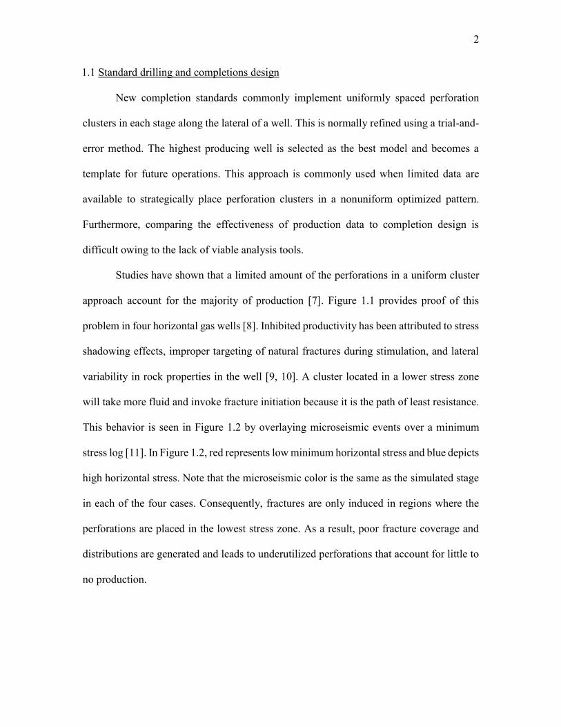
1.5 Thesis overview
This thesis presents the results of simulations of a number of horizontal multistage
well designs in an oil reservoir. The simulations are original in that they used a combination
of discrete fracture modeling software packages. The chapters in this thesis are as follows:
Chapter 2 begins with the theory used in the unconventional fracture model (UFM),
accounting for hydraulic and natural fracture interaction, stress shadowing effects, and the
governing equations for hydraulic fracture propagation.
Chapter 3 includes the workflow progress with input parameters pertaining to the wellbore
design, stochastic natural fracture set generation and validation, rock properties based on
logging and core data, and the pump schedule.
Chapter 4 presents the UFM simulation results and also compares six-month production
data of three nearby horizontal wells with differing completions designs.
Chapter 5 concludes the thesis project and provides suggestions for future studies.

7
Figure 1.1. Production data of four horizontal gas wells. Results indicate that multiple perforation clusters are producing little to no gas due to poor spacing design.

8
Figure 1.2. Microseismic event overlaying a minimum stress log. Regions of red indicate low stress and blue represents high stress.
Table 1.1: List of common diverting agents and their drawbacks
Diverting Agent Drawbacks
Ball Sealers
Cannot be used for open hole wells Requires constant pressure for balls to remain seated Inefficient when perforations erode Degradation time must be accurate or efficiency severely drops
Benzoic acid flakes Very brittle and can break during pumping Gilsonite Mesh sizes are typically too high to bridge wellbore widths
Rock Salt Dissolution rate is highly dependent on formation salinity Requires saturated brine as a pump fluid Requires special surface storage tanks
Wax beads Applicable only in low temperature wells (<180⁰ F)

CHAPTER 2
UNCONVENTIONAL FRACTURE MODEL
METHODOLOGY
Satisfying the objectives of this study requires the construction of a geomechanical
model using commercial software that can infer the extent of in-situ natural fracturing,
comprehend production changes based on cluster perforation design, and assess the
effectiveness of diversion in fracture stimulation. No one numerical simulator can currently
fulfill these needs without manipulating the model. The model is altered by utilizing the
capabilities of two complex fracture simulators in tandem. FracMan — developed by
Golder Associates — is used for building and validating the framework of the model. It is
one of the more efficient platforms for stochastically representing natural fractures.
FracMan’s well and natural fracture sets were imported into Mangrove, and populated with
the necessary parameters to simulate the effects of a complex natural fracture system.
Mangrove’s unconventional fracture model (UFM) simulates fracture stimulation,
deformation, fluid flow, and proppant transport within a natural fracture system. The
interactions between hydraulic and natural fractures considered by implementing a
crossing algorithm developed from experimental work by Renshaw and Pollard [20]. The
solutions to fluid flow and elastic deformation are similar to the governing equation of a
pseudo-3D discrete fracture model. The major difference of the UFM is solving the

10
problems with multiple fractures. Figure. 2.1 illustrates the difference between a planar
fracture and complex fracture simulation. Accounting for the behavioral effects of natural
fractures in the UFM require modifications to existing fracture modeling equations used in
traditional simulators and the inclusion of new solutions. The remaining sections in Chapter
2 focus on the new and modified solutions used to construct UFM.
2.1 Governing equations
The governing equations account for the physical processes affecting fracture
propagation. This includes fracture deformation mechanics, fluid flow behavior, and
fracture propagation criterion. The horizontal wells assessed contain mainly vertical natural
fractures (discussed further in the FMI analysis chapters) and are within reason when
applied to the UFM. The basic governing equations consist of seven equations listed as
follows:
Fracture power-law fluid flow
1'
1'201
n
flfln H
q
H
q
ws
p (2.1)
'
'0 '2'4
)'('2 n
n n
n
n
K
; dzw
zw
Hn
n
n
Hfl
fl
'1'2
)(1)'(
The Poiseulle equation determines fluid flow in each fracture element. It is not limited to
power-law behavior. Newtonian fluid behavior, slickwater for example, may be considered
for the case of n’=K’=1. Fluid characteristics are discussed further in section 3.4.

11
p ......................................................................................................... Fluid pressure
q ...................................................................................................... Local flow rate,
Hfl ...................................................................... Height of the fluid in the fracture,
w ..................................................................................................... Average width,
n' .................................................................................................. Power-law index,
K ................................................................................................ Consistency index,
s ..................................................................................... Distance along the fracture
Local mass balance
0)(
L
flq
t
wH
s
q
(2.2)
0)(
L
flq
t
wH
s
q
The local mass balance accounts for every fracture. Based on poststimulation reports and
diagnostic fracture injection tests (DFIT), the efficiencies were high and the leakoff
coefficient was negligible. Sections 3.2 and 3.4 will elaborate more on this observation.
CL ............................................................................................. Leakoff coefficient,
hL ............................................................................................ Leakoff zone height,
τ0(s) ......................................Time when each fracture element is exposed to fluid
Global volume balance
t tL
H
tL t
lL
L
dtdsdhqdswHdttQ0
)(
0
)(
0 0
)( (2.3)
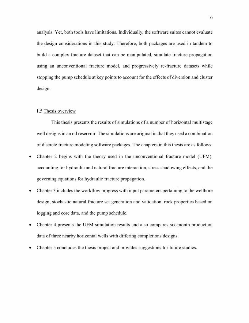
12
Q(t) ................................................................................................ Total pump rate,
L(t) ...................................................... Summation of all fracture lengths at time t,
H(s,t) .............................................. Fracture height at a point in a fracture at time t
Sum local flow rate
i
perfi NitQtq ,..1),()( (2.4)
q(t) .......................................................... Local injection rate into each perforation
Fracture width
),),,((),,( zHyxpwzyxw (2.5)
A 2D plane strain solution for fracture widths is used, and performs similar to a
cell-based pseudo-3D model, for the sake of computational efficiency. Vertical and
horizontal fracture growth for a pseudo-3D case is considered separately and calculated
from a local pressure and vertical stress profile. However, this approach requires fracture
initiation and propagation to remain in the lowest stress zone. In this study, some of the
cluster perforations of the proposed wells lie in higher stress layers and will eventually
break into lower stress regions. This causes inaccurate accounting of fracture height growth
and requires a more feasible approach. Consequently, a “Stacked Height Growth” model
is integrated into the UFM a discussed further in section 2.2.
13
2D PKN width
'2)(
E
pHw n (2.6)
E’ .............................................................................. Plane strain Young’s modulus
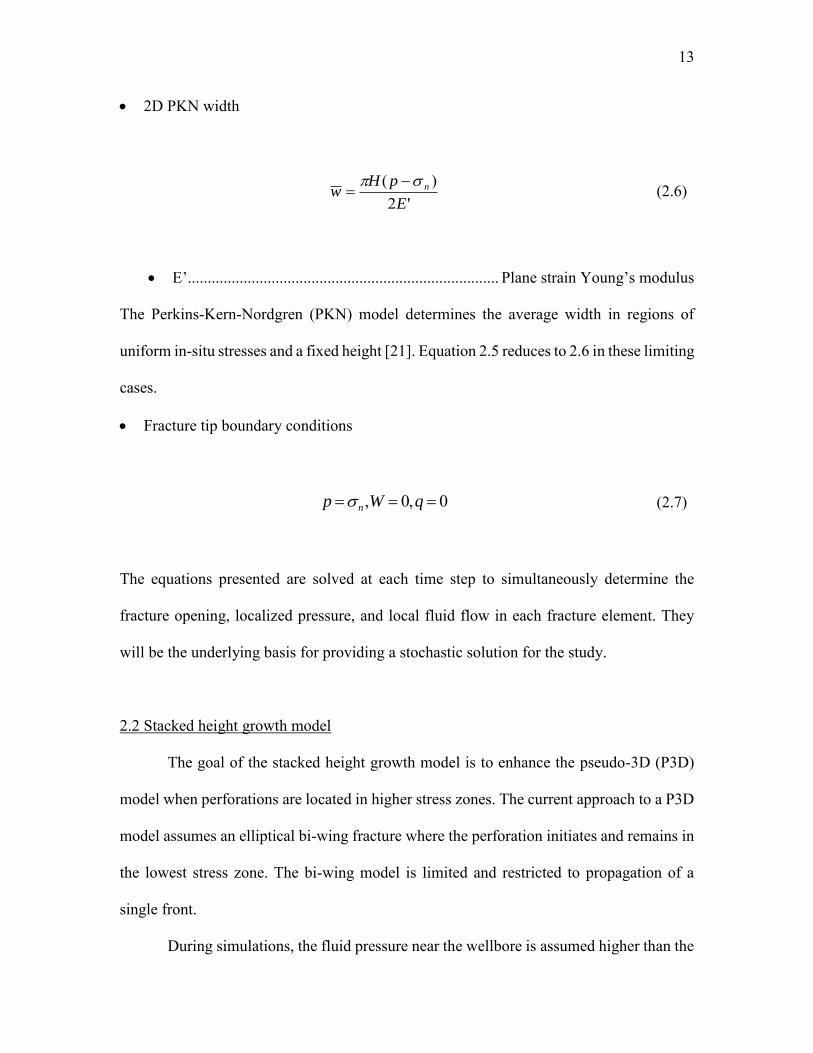
The Perkins-Kern-Nordgren (PKN) model determines the average width in regions of
uniform in-situ stresses and a fixed height [21]. Equation 2.5 reduces to 2.6 in these limiting
cases.
Fracture tip boundary conditions
0,0, qWp n (2.7)
The equations presented are solved at each time step to simultaneously determine the
fracture opening, localized pressure, and local fluid flow in each fracture element. They
will be the underlying basis for providing a stochastic solution for the study.
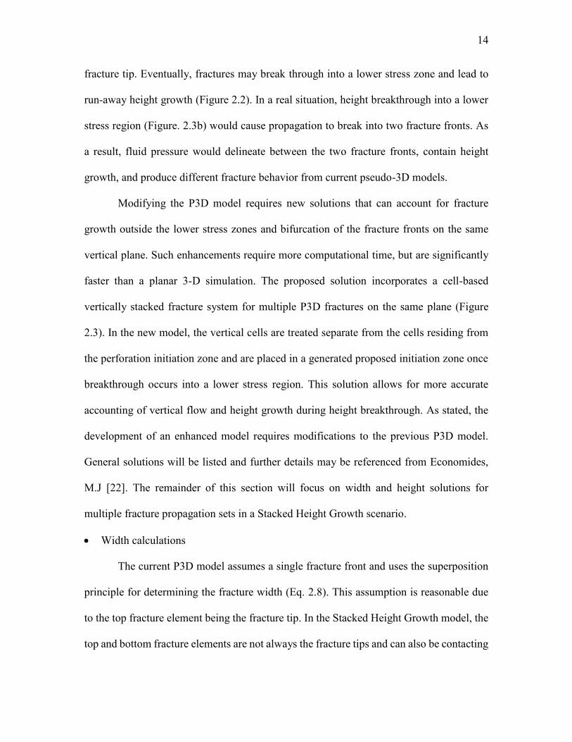
2.2 Stacked height growth model
The goal of the stacked height growth model is to enhance the pseudo-3D (P3D)
model when perforations are located in higher stress zones. The current approach to a P3D
model assumes an elliptical bi-wing fracture where the perforation initiates and remains in
the lowest stress zone. The bi-wing model is limited and restricted to propagation of a
single front.
During simulations, the fluid pressure near the wellbore is assumed higher than the
14
fracture tip. Eventually, fractures may break through into a lower stress zone and lead to
run-away height growth (Figure 2.2). In a real situation, height breakthrough into a lower
stress region (Figure. 2.3b) would cause propagation to break into two fracture fronts. As
a result, fluid pressure would delineate between the two fracture fronts, contain height
growth, and produce different fracture behavior from current pseudo-3D models.
Modifying the P3D model requires new solutions that can account for fracture
growth outside the lower stress zones and bifurcation of the fracture fronts on the same
vertical plane. Such enhancements require more computational time, but are significantly
faster than a planar 3-D simulation. The proposed solution incorporates a cell-based
vertically stacked fracture system for multiple P3D fractures on the same plane (Figure
2.3). In the new model, the vertical cells are treated separate from the cells residing from
the perforation initiation zone and are placed in a generated proposed initiation zone once
breakthrough occurs into a lower stress region. This solution allows for more accurate
accounting of vertical flow and height growth during height breakthrough. As stated, the
development of an enhanced model requires modifications to the previous P3D model.
General solutions will be listed and further details may be referenced from Economides,
M.J [22]. The remainder of this section will focus on width and height solutions for
multiple fracture propagation sets in a Stacked Height Growth scenario.
Width calculations
The current P3D model assumes a single fracture front and uses the superposition
principle for determining the fracture width (Eq. 2.8). This assumption is reasonable due
to the top fracture element being the fracture tip. In the Stacked Height Growth model, the
top and bottom fracture elements are not always the fracture tips and can also be contacting

15
other elements. Therefore, Eq. 2.8 is modified into the form of Eq. 2.9. Detailed solutions
of Eq. 2.9 can be referenced in Appendix A.
1
1
1
1
2cos)(
2
cosh)()(
'4)()(
'4)(
n
i
i
i
i
i
iicpfncp
h
hharzhz
hz
hh
hhz
zh
Ezhzzhgp
Ezw
(2.8)
Nstack
j
H
H
jcpjfjcp
j
j
daaz
ah
ahz
aahgPE
zhw1
1,,,
1||
2
cosh)()(4),(
(2.9)
w(h,y) ........................ Width profile at given depth and distance from perforation,
j ...................................................................................... Reference element integer,
hcp,j .............................................................................................. Reference depth,
σ(a) ....................................................................................... Element in-situ stress,
Pcp ............................................ Pressure in the fracture at a reference depth hcp,j,
𝜌cp,j .......................................................... Fluid density at a reference depth hcp,j,
g .................................................................................................................. Gravity,
h ...................................................................................................... Fracture height,
H .............................................................................. Height of the stacked element,
a ...................................................................... Element height as a function of Hj,
z ....................................................................................................................... Depth

16
Height growth
Height growth is calculated based on the top and bottom intensity factor of a
fracture. Eq. 2.10a and 2.10b define intensity solutions in Mangrove.
1
1!
)(
2arccos22)
43(2 n
i
ii
i
iincpcpIup
hhh
h
hhh
hhhgP
hK
f
(2.10a)
1
1!
)(
2arccos22)
4(2 n
i
ii
i
iincpcpIup
hhh
h
hhh
h
hhgP
hK
f
(2.10b)
Similar to the width equations, the stress intensity factors are calculated based on the local
pressure and stress along the entire fracture cross section. The stacked height growth model
makes adjustments by calculating the stress intensity for each stacked element in the cross
section (Eq 2.11a and 2.11b). Detailed solutions of the new stress intensity equations are
listed in Appendix B.
Nstack
j
H
H
jcpjfjcpIup
j
j
daah
aaahgP
hK
1,,,
1
)()(2
(2.11a)
Nstack
j
H
H
jcpjfjcpIdown
j
j
daah
aaahgP
hK
1,,,
1
)()(2
(2.11b)

17
The stacked height growth equations are an improvement compared to the
limitations observed in a P3D model. Fracture prediction is less accurate than a planar 3D
model, but requires less computation time and simulates fracture behavior within reason.
For this study, the stacked height growth option will be used within Schlumberger’s
Mangrove software package and predict accurate fracture propagation when perforations
are located in higher stress layers.
2.3 Hydraulic and natural fracture interaction
The main draw to using Mangrove’s unconventional fracture model is the ability to
solve fracture propagation problems related to a complex natural fracture system.
Furthermore, the tool accounts for the interactive behavior when a hydraulic fracture
approaches a natural fracture. This is an important consideration with the existence of
naturally fractured reservoirs.
The behavior between hydraulic and complex fractures is a very complex process
and one of the core reasons for the creation of a complex fracture system. A stress field
exists at the tip of a hydraulic fracture. Several propagation events may occur based on the
magnitude of the stress field and geomechanical properties of existing natural fractures.
Figure 2.4 illustrates possible event paths [23]. Three possible propagation cases exist:
1) Fracture tip pressure is not high enough to overcome the minimum in-situ stresses and
slips, causing dilation in the natural fracture (2.4d)
2) The hydraulic fracture crosses the natural fracture and remains planar (2.4e)
3) Fluid pressure is high enough for crossing and slippage (2.4f)
Each of the three behaviors may change due to fluid pressure variation during pumping. A

18
crossing criterion considering the cases listed has been developed by Gu and Weng based
of experimental work by Renshaw and Pollard [20, 23]. This criterion considers rock
characteristics, rheological properties, leakoff 18ffects, and the angles of interaction.
Crossing criterion
The natural fractures are considered interfaces when addressing mechanical
interactions with hydraulic fractures. The angle of intersection between a hydraulic fracture
and natural fracture is β (Figure 2.5). The stress field of the in-situ and shear stresses σh,
σH, and τxy is defined by the following:
23sin
2sin1
2cos
21
r
KHx
(2.12)
23sin
2sin1
2cos
21
r
Khy
23sin
2cos
2sin
21
r
Kxy
K1 ......................................................................................... Stress intensity factor,
r ........................................................................................................... Polar length,
θ ............................................................................................................ Polar angle
Crossing the natural fracture interface requires the maximum principal stress σ1 to be equal
to the rock tensile strength:
19
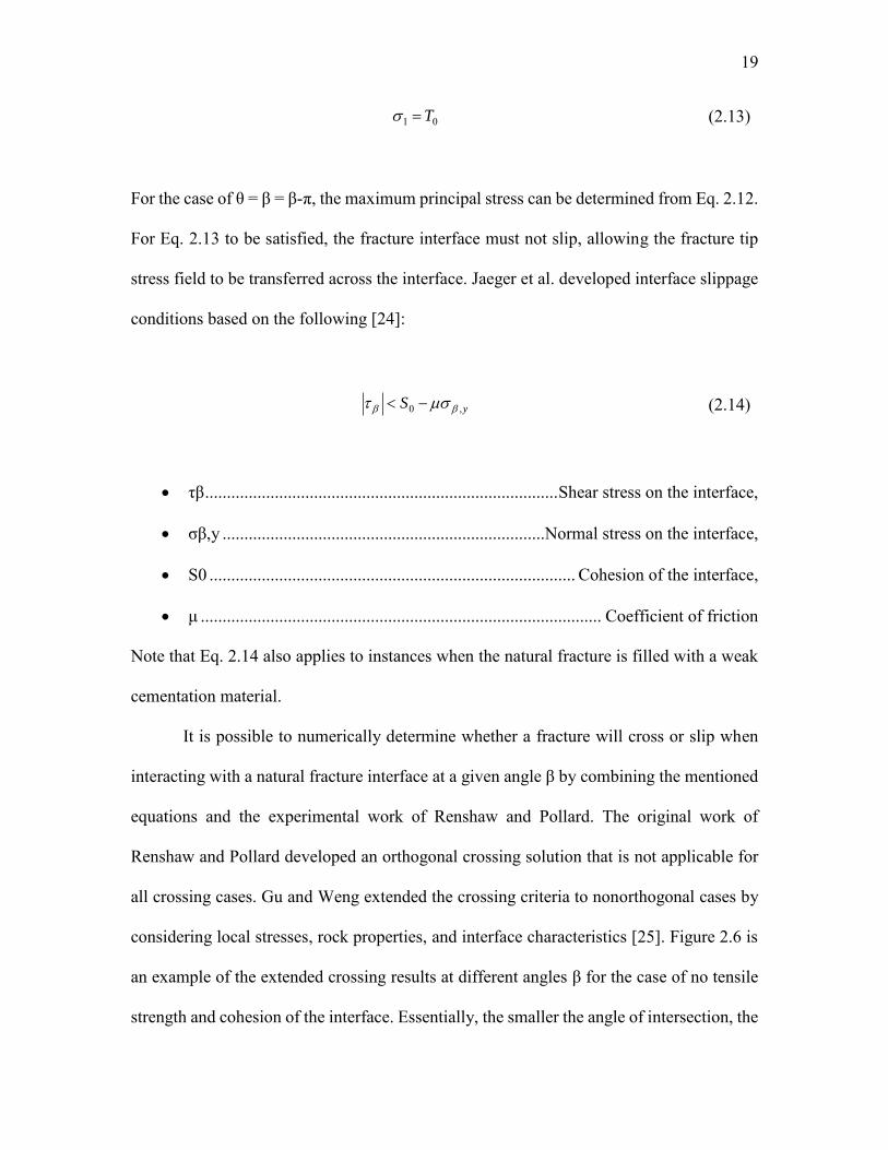
01 T (2.13)
For the case of θ = β = β-π, the maximum principal stress can be determined from Eq. 2.12.
For Eq. 2.13 to be satisfied, the fracture interface must not slip, allowing the fracture tip
stress field to be transferred across the interface. Jaeger et al. developed interface slippage
conditions based on the following [24]:
yS ,0 (2.14)
τβ ................................................................................. Shear stress on the interface,
σβ,y ..........................................................................Normal stress on the interface,
S0 .................................................................................... Cohesion of the interface,
μ ............................................................................................ Coefficient of friction
Note that Eq. 2.14 also applies to instances when the natural fracture is filled with a weak
cementation material.
It is possible to numerically determine whether a fracture will cross or slip when
interacting with a natural fracture interface at a given angle β by combining the mentioned
equations and the experimental work of Renshaw and Pollard. The original work of
Renshaw and Pollard developed an orthogonal crossing solution that is not applicable for
all crossing cases. Gu and Weng extended the crossing criteria to nonorthogonal cases by
considering local stresses, rock properties, and interface characteristics [25]. Figure 2.6 is
an example of the extended crossing results at different angles β for the case of no tensile
strength and cohesion of the interface. Essentially, the smaller the angle of intersection, the

20
more difficult it becomes for crossing to occur. Additionally, the angle of intersection is a
very sensitive parameter in determining the crossing criteria.
The extending nonorthogonal criterion presented has been validated by
experimental work and quantitatively accounts for whether crossing or slippage will occur
[20, 23, 25]. The criterion requires the use of a numerical simulator that accounts for each
of the mentioned parameter inputs. Mangrove’s UFM implements the crossing behavior
defined and accounts for natural fracture effects during hydraulic fracture stimulation.
2.4 Stress shadowing effects
Fracture propagation is highly dependent on the mechanical interactions between
nearby hydraulic and natural. Interaction consider nearby fracture stress fields generated
by each fracture being displaced due to opening or shearing. For the case of a 3D, plane-
strain, displacement discontinuity solution, Olson et al. (2004) improved on the solution
provided by Crouch and Starfield describing the normal and shear stresses acting on a
fracture element due to opening and shearing of other nearby elements (Eq. 2.15) [26, 27].
N
j
jn
ijnn
ijN
j
js
ijns
ijin DCGDCG
11 (2.15)
N
j
jn
ijsn
ijN
j
js
ijss
ijis DCGDCG
11
ijnsC ....................... Normal stress at i from a shear displacement discontinuity at j,
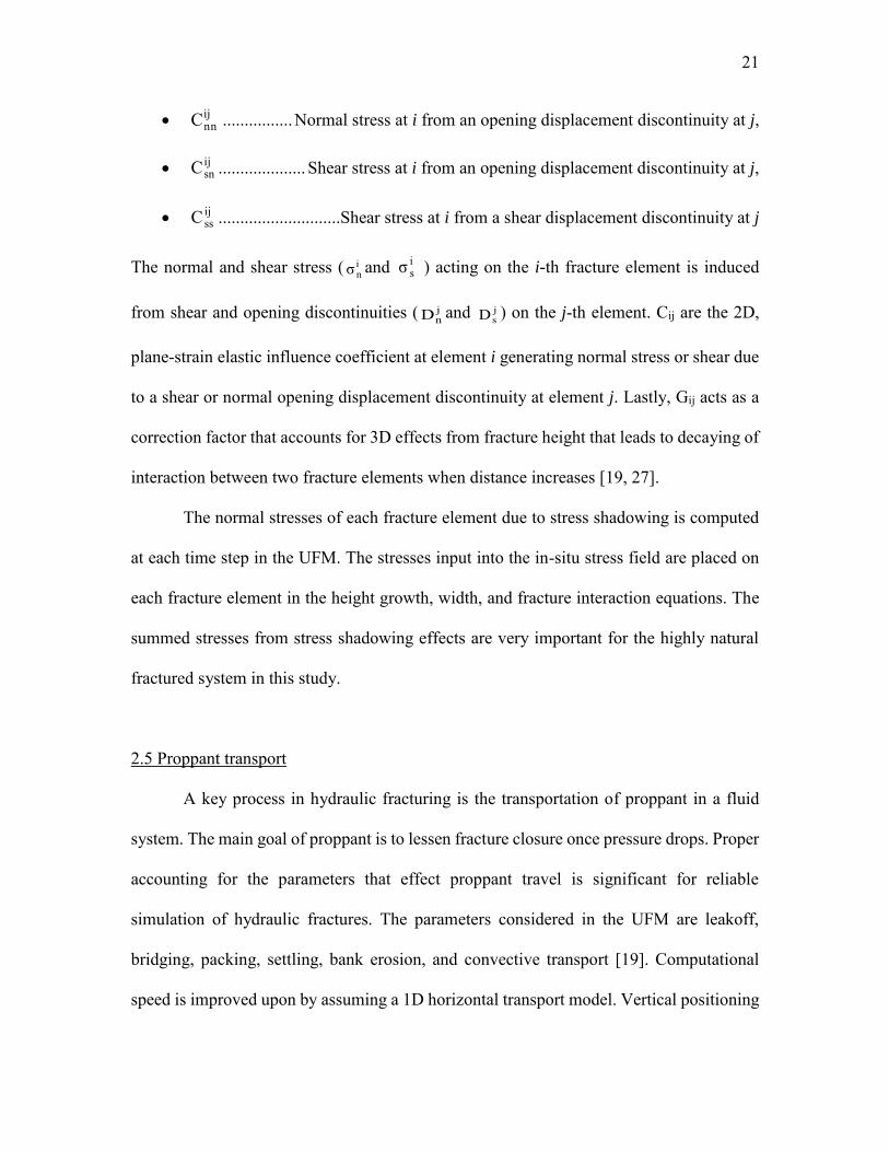
21
ijnnC ................ Normal stress at i from an opening displacement discontinuity at j,
ijsnC .................... Shear stress at i from an opening displacement discontinuity at j,
ijssC ............................Shear stress at i from a shear displacement discontinuity at j
The normal and shear stress ( inσ and i
sσ ) acting on the i-th fracture element is induced
from shear and opening discontinuities ( jnD and j
sD ) on the j-th element. Cij are the 2D,
plane-strain elastic influence coefficient at element i generating normal stress or shear due
to a shear or normal opening displacement discontinuity at element j. Lastly, Gij acts as a
correction factor that accounts for 3D effects from fracture height that leads to decaying of
interaction between two fracture elements when distance increases [19, 27].
The normal stresses of each fracture element due to stress shadowing is computed
at each time step in the UFM. The stresses input into the in-situ stress field are placed on
each fracture element in the height growth, width, and fracture interaction equations. The
summed stresses from stress shadowing effects are very important for the highly natural
fractured system in this study.
2.5 Proppant transport
A key process in hydraulic fracturing is the transportation of proppant in a fluid
system. The main goal of proppant is to lessen fracture closure once pressure drops. Proper
accounting for the parameters that effect proppant travel is significant for reliable
simulation of hydraulic fractures. The parameters considered in the UFM are leakoff,
bridging, packing, settling, bank erosion, and convective transport [19]. Computational
speed is improved upon by assuming a 1D horizontal transport model. Vertical positioning

22
of the proppant bank, slurry, and clean fluid are computed in each fracture element.
The numerical implementation of fluid and proppant transport in the UFM
determines the material locations within each fracture element at explicit time steps.
Proppant transport are determined from volumetric concentration of the fluid and proppant
components averaged over the element volume above the proppant bank (Eq. 2.16)
H
H
w
w
xx
xx
k
bank
k
bank
c
c
dzdydxzyxXHHwx
c2
2
2
2
'
''
''
''),','()(
1 (2.16)
Xk ............................... Volume fraction of fluid or proppant identified by index k,
Δx’ .................................................................... The length of the fracture element,
xc ........................................................................ Fracture element reference length,
H ............................................................................. Height of the fracture element,
Hbank ......................................................................... Height of the proppant bank,
ck .............................. Concentration of the fluid of proppant identified by index k,
w ................................................................. Average width of the fracture element
Being able to account for the volumetric concentration proppant within each fracture
element is essential. Diverter will be simulated as “proppant” and be used to determine the
fractures containing the majority of proppant during certain stages of a pump schedule. The
process of modeling diversion will be elaborated on more in section 3.4.
The settling velocity for solids is determined by the Stoke’s law solution for power
law fluids presented by Daneshy [24]:

23
'1
1',1', '183
1 nnk
flkprop
nkset gDK
v
(2.17)
vset,k ........................................................... Settling velocity for proppant index k,
'n ............................................................................ Averaged flow behavior index,
'K ...................................................................... Averaged flow consistency index,
g .................................................................................................................. Gravity,
𝜌prop,k ..................................................... Proppant density identified by index k,
Dk ............................................................. Proppant diameter identified by index k
fl ............................................................... Settling velocity for proppant index k
Multiple proppant materials are available in Mangrove’s database. Also, custom fluid and
proppant types can be added if the K’, n’, diameter, and density values are known
24
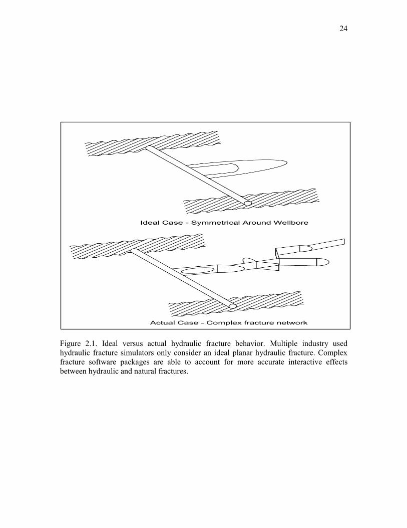
Figure 2.1. Ideal versus actual hydraulic fracture behavior. Multiple industry used hydraulic fracture simulators only consider an ideal planar hydraulic fracture. Complex fracture software packages are able to account for more accurate interactive effects between hydraulic and natural fractures.

25
Figure 2.2. Perforation examples in a lower (a) and higher (b) stress zone. Perforations are located outside the lowest stress zone in both instances. The P3D model commonly leads to two common growth occurrences: 1) runaway height growth and 2) uncorrected height growth. The fracture is more likely to be contained or split into more than one propagation front in realistic occurrences (proven from planar 3D simulations).

26
Figure 2.3. Stacked height growth model example illustration. The original injected perforation and eliminated and two new injection points are generated in locations containing the lowest stress zone. It is possible for splitting to occur again if the new injection zones have height growth into other lower stress zone.

27
Figure 2.4. Possible hydraulic fracture and natural fracture interactive pathing (modified from Gu, H. et al. (2011) [23]).
28
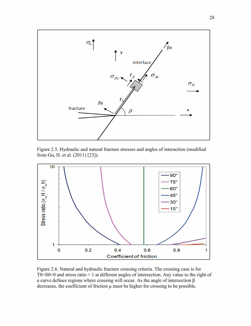
Figure 2.5. Hydraulic and natural fracture stresses and angles of interaction (modified from Gu, H. et al. (2011) [23]).
Figure 2.6. Natural and hydraulic fracture crossing criteria. The crossing case is for T0=S0=0 and stress ratio > 1 at different angles of intersection. Any value to the right of a curve defines regions where crossing will occur. As the angle of intersection β decreases, the coefficient of friction μ must be higher for crossing to be possible.

CHAPTER 3
STOCHASTIC MODEL ASSEMBLY
Understanding the subsurface geology is vital in constructing an accurate discrete
fracture network (DFN) model. The model will act as the core testing component when
analyzing parameter variations in pump schedules and completions designs. It is important
that field data provide adequate information to build a model similar to actual geologic
structures and their associated mechanical properties.
The first six to eight months of the project focused on data collection and analysis.
Subsurface data consisted of:
Well logs
Lateral FMI logs
Diagnostic fracture injection tests
Drilling completion reports
Geosteering reports
Core tests
The information originated from three near-field wells and the three test wells. The near-
field wells produce from the same reservoir as the test wells. However, depositional shifts
in the lithology is present and will require calibration to the test wells.
Chapter 3 focuses on the approach to building a stochastic model by processing
30
available field data. Other important components relating to the drilling and completions
planning process are not addressed in this document. However, they are still important
operational challenges to consider outside the scope of this project. Additional publications
can be found in published literature [29-31].
3.1 Well construction
The initial workflow process in FracMan and Mangrove require the construction of
a subsurface well. Geosteering and survey reports were available for one wellhead
containing three lateral sections. For proprietary purposes, the wells designations are test
well 1, 2, and 3 and contain the following design:
Test Well 1 – Limited entry design
Test Well 2 – Standard completions design
Test Well 3 – Standard completions design
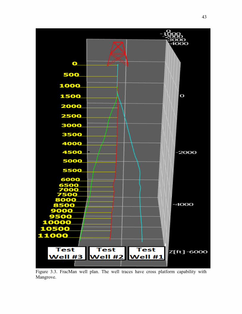
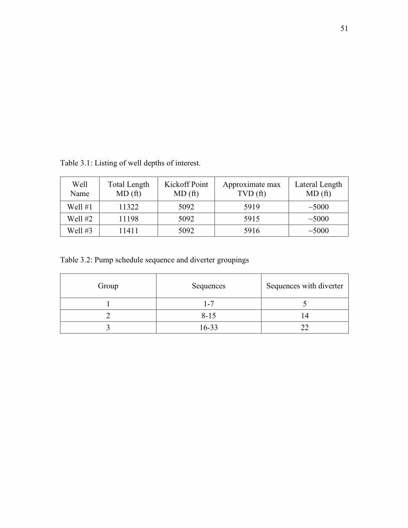
Figure 3.1 and 3.2 provided Schematics of the wells. Table 3.1 lists approximate depths,
kick-off points, and lengths of the laterals. A well model has been built from referenced
geosteering coordinates and tested cross platform between the two fracture simulator
packages (Figure. 3.3). Wellhead locations and depths are exact and remain fixed for the
entirety of the simulation process.
3.2 Well logging overview
Well placement is highly dependent on petrophysics. It may not be something a
drilling and completions engineer is directly involved in. However, it is key to understand
how well logging data leads to preplanning designs and corrections during drilling.
31
Wireline instruments were run down the hole on an electric cable to perform well
logging after drilling the well. Open-hole (casing and cement not yet placed) logging was
conducted on the test well. The remaining sections provide a general summary of the types
of well logs issued and how they affected design choices for the stochastic model.
Gamma ray
Rocks contain natural occurring radioactive material mostly consisting of
potassium, uranium, and thorium. Gamma ray tools measure the amount of natural gamma
rays emitted by the rock surrounding the tool. The unit of measurement is API or GAPI, a
unit based off the radiation of a concrete block that is nearly twice the radioactivity of any
shale rock. It is probably the most commonly used tool for determining changes in
lithologic zones. Generally, the gamma ray value is said to be proportional to the amount
of shale in the rock. As a rule of thumb, a higher gamma ray means more shale. A spectral
gamma ray was also available. The composite results showed nearly the same output as the
basic gamma ray, meaning no radioactive discrepancies were present in the logged
formations.
Density log
Density logging also utilizes gamma rays by sending a gamma ray into a formation
and recording the amount scattered back. The average electron density in a formation
dictates the amount of gamma rays scattered back to the tool. The electron density strongly
correlates to the bulk density of the material. A correlation can be made between the
scattered gamma ray and bulk density of the nearby rock formation. The unit of
measurement for bulk density is in g/cc. Density logging was also used to calculate the
density rock porosity.

32
Resistivity log
Resistivity logging measures the electrical resistivity of a rock by recording how
much a material opposes the flow of electrical current. Resistivity uses multiple pads to
eliminate the resistance of the contact leads. The unit of measurement is in Ohms.
Hydrocarbons increase resistivity more compared to water. The following provides a
general rule:
High resistivity high porosity –Likely hydrocarbon
Low resistivity high porosity – Likely shale or water
Neutron log
The neutron-porosity logging is a simple tool. It uses an isotopic source and two
neutron detectors similar to density logging. The tool measures the size of the neutron cloud
by characterizing the falloff of neutrons between the two detectors. The log targets the
average hydrogen density of the material logged. The hydrogen index will track the
porosity if all the hydrogen in the formation is in the form of porosity-filling liquid (in
particular water or oil).
The density and neutron porosity logs are overlaid on the same track. The key areas
of interpretation are regions where the neutron and density porosity logs cross over.
Hydrocarbons exist in the zone where the resistivity is high and the porosity logs cross
over.
Sonic log
Sonic logs measure the interval transit time of a formation. The transit time
describes a formation’s capacity to transmit seismic waves. Seismic wave travel speeds
will vary with lithology and rock textures. Travel time is typically faster as rock density

33
increases. A shear and compressional travel time value was measure and provided. With
these data and density logs, geomechanical properties such as Young’s modulus, Poisson’s
ratio, and the in-situ stresses can be solved.
Logging gives valuable information on every formation logged. This information
aids in preplanning and optimization during drilling. Logging provides the information
necessary for the following:
Identify subsurface formations and their thicknesses
Estimate regions with gas and oil in place
Determine geomechanical rock properties
Choose proper casing placement
3.3 Stratigraphy
Subsurface model layers were built based on user selected interval changes from
the gamma ray. Vertical openhole logs were not run in the test wells. Consequently,
available vertical well data were given from three nearby wells designated as near-field 1,
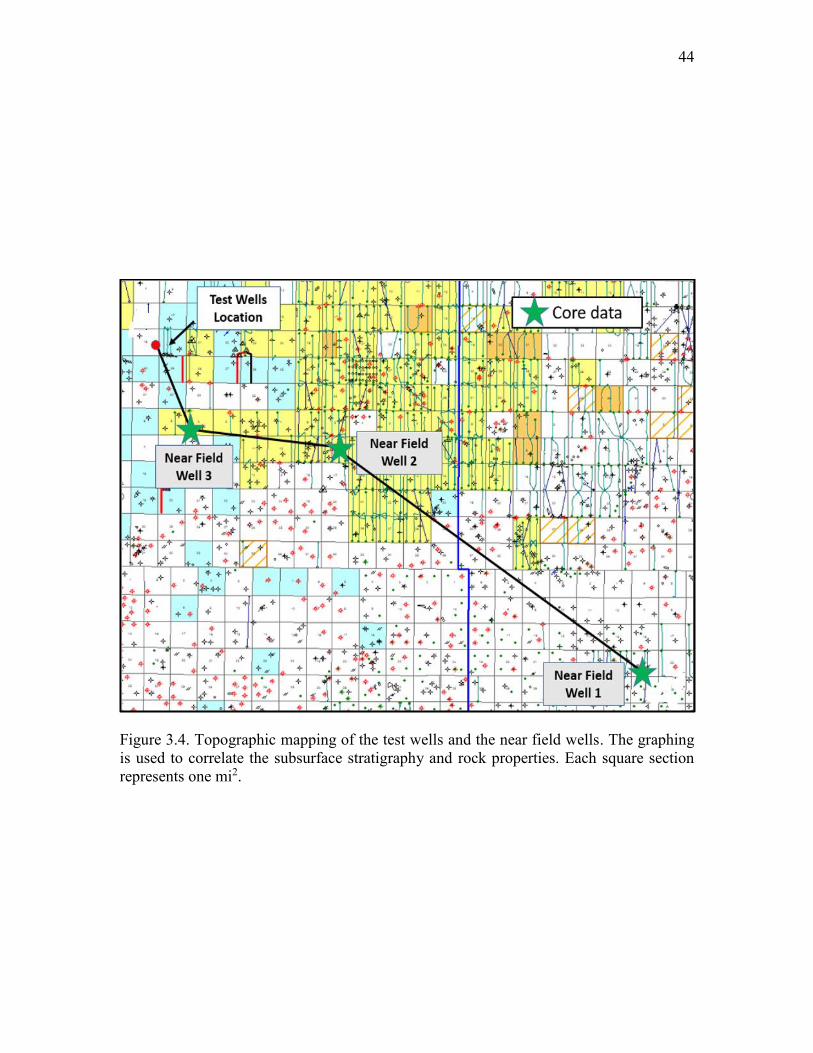
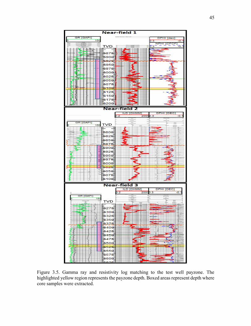
2, and 3. Figure 3.4 provides a map of the location of the wellheads. Gamma ray
correlations of the near-field wells are illustrated in Figure 3.5. The yellow line represents
the known payzone depth that is used as the matching region between logs. The boxed
regions are where core samples were extracted. The objective consisted of matching the
gamma rays of the near-field wells to the test well mud log, verifying that the gamma ray
patterns are similar between wells, and picking stratigraphic changes as a function of depth.
Mangrove and FracMan require the user to input the TVD and the thickness of each
formation. The operator engineers and geologists suggested a simple lithological model

34
100 ft. above and below the payzone. The decision was based on fracture height growths
from previous stimulation jobs not escalating above 50 ft and below 20 ft. The hindrance
in height growth is possibly be due to lamination effects. It requires a high amount of
energy to vertically fracture through additional beddings. Multiple interbedded formations
were observed from the gamma ray logs. Thirty layers were identified ranging from 5-20
ft in bedding thickness within the 200 ft interval. Figure 3.6 illustrates a side view of the
vertical stratigraphy matched to the test wells. The next step requires populating the layers
with geomechanical properties.
3.4 Rock properties
Goemechanics is a fundamental building block in drilling and completions, yet not
fully utilized in drilling and completions. This may be due to limited availability in well
logs necessary to perform petrophysical analysis. Understanding the mechanical behavior
of a rock allows an engineer to make reasonable influential choices during phases of
completion, stimulation, and production.
Rock characteristics were loaded into the layers surrounding the lateral. As a result,
the containing layer rock property data are used in the equations defined in Chapter 2
during each time step of the simulation. The properties input into stratigraphic zones were:
Minimum horizontal stress(σ3)
Maximum horizontal stress(σ2)
Overburden stress (σ1)
(σ1) Trend/plunge
(σ3) trend/plunge

35
Young’s Modulus
Poisson’s ratio
The methods to calculating each value are listed in the following sections. Petrophysical
analysis techniques are referenced from Crain’s Petrophysical Handbook [32].
Poisson’s ratio
1
15.0
2
2
DTC
DTS
DTC
DTS
v (3.1)
ν......................................................................................................... Poisson’s ratio
DTS ................................................................ Compressional travel time (μsec/ft),
DTC ................................................................................ Shear travel time (μsec/ft)
Shear modulus
2400,13
DTS
RHOBG (3.2)
G .................................................................................... Shear modulus (x106 psi),
RHOB ......................................................................... Formation density log (g/cc)

36
Young’s modulus
12GE (3.3)
E .................................................................................. Young’s modulus (x106 psi)
Bulk modulus with porosity
22
1431*400,13
DTSDTCRHOBKb (3.4)
Kb ................................................................. Bulk density with porosity (x106 psi)
Bulk modulus with no porosity
PHIT
DENSWPHITRHOBDENSMA
1*
(3.5a)
PHIT
DTWPHITDTCDTCMA
1*
(3.5b)
PHIT
DTSDTSMA
1
(3.5c)
22
1431*400,13
DTSMADTCMADENSMAKm
(3.5d)

37
Km ..........................................................Bulk density without porosity (x106 psi),
PHIT ................................................................................. Total porosity (fraction),
DENSW ............................................. Density of the fluid in the rock pores (g/cc),
DTW ................................ Travel time through the fluid in the rock pores (μsec/ft)
Biot’s constant
m
b
K
KB 1 (3.6)
B ........................................................................................Biot’s constant (unitless)
Overburden pressure gradient
DEPTH
INCRRHOBSUM iv
)*(*0605.0 (3.7)
σv ................................................................. Overburden pressure gradient (psi/ft),
RHOBi ................................. Formation density log reading at i-th data point(g/cc)
INCR .................................................................. Digital log data incriment (psi/ft),
,DEPTH ..................................................................................... Logging depth (ft)
Pore pressure gradient
DEPTH
DENSWpore (3.8)

38
σpore ........................................................................ Pore pressure gradient (psi/ft),
RHOBi ................................. Formation density log reading at i-th data point(g/cc)
Minimum stress gradient
poreporev BB
**
1min
(3.9)
σmin .................................................... Minimum horizontal stress gradient (psi/ft)
Maximum stress gradient
Correction*minmax (3.10)
σmax ................................................... Maximum horizontal stress gradient (psi/ft)
Rock properties were calculated from near-field well 3 and correlated to the test wells.
Figures 3.8, 3.9, and 3.10 provide values for the Poisson’s ratio, Young’s modulus, and
minimum horizontal stress. Regions with no data or outliers are locations where logging
stopped. Instances with no data required referencing from the core samples and DFIT
reports. The most important region, the payzone, was one of these cases. However, rock
core samples were extracted at the payzone depths and tested (red region Figure 3.10).
The geomechanical properties were within reason compared to the logging calculations.
Final rock values were integrated into the layer properties used for later simulations.

39
3.5 Complex natural fracture sets
Halliburton provided the fracture count and orientation data processed from the
FMI logs from test well 2. Approximately 1800 conductive fractures (fractures of interest)
exist in the lateral. No noticeable faults were identified in this area of the field. The fracture
orientations fall into two major groups: NW and SE groupings (conjugate fracture
systems). The fracture set data were uploaded into FracMan and verified using a stereonet
plot and Rose plot comparison between the raw Halliburton data and statistically generated
fractures (Figure. 3.7). Then, the fracture set mean pole/trend was approximated. The
accuracy of the mean pole/trend calculated from the data was validated by running an
internal FracMan routine. The algorithm is a probabilistic pattern recognition algorithm
that defines fracture sets from field data.
The actual fracture data are not used for simulations in FracMan. The software
requires a theoretical fracture set to be statistically generated from user-defined input. The
fracture sets required inputs for the fracture intensity (P10) and mean pole/trend. Two
fracture sets were produced using the data input from the Halliburton FMI evaluations.
The fracture sets are generated in a bounded region. In this instance, the selected
region surrounded the lateral section of the well. The statistical routine in FracMan
generated approximately 100,000 – 250,000 fractures. The region was filtered to only
include fractures that directly connected to the well. The filtered connected fracture set
count and location was nearly identical to the conductive fractures input from the FMI data,
as would be expected. Essentially, a realistic set of natural fractures was generated along
the length of the wellbore. Figure 3.8 shows a 2-dimensional visualization of the fractures
that were generated along the length of the wellbore and imported Mangrove.

40
3.6 Completions and treatment design
The baseline treatment design was copied from postfracture reports for well 1, 2,
and 3. To avoid confusion, each isolated and perforated well section that is treated
individually will be called a stage. Steps in the treatment schedule where there is a change
in rate, fluid, additives, or solids added is classified as a sequence. The treatment schedule
consisted of 33 sequences including HCl, slickwater, and HCl-gelled acids, diverter, and
perforation plugging materials. Sequences were placed into three groupings (Table 3.2).
The fracture design used Ranch House medium rock salt as diverting agent.
Diverter was pumped in sequences 5, 14, and 22 (Table 3.2). Diversion is not specifically
represented in this or other multiple fracture simulators and required some creative (but
rational) simulations. Diversion was numerically modeled by pumping proppant with
similar size and density of the rock salt. The simulation is temporarily terminated and
properties are recorded in fractures taking fluid and proppant once fluid is finished
pumping through a grouping. Fractures that took proppant were eliminated (i.e., no further
injection will occur into those because they have been assumed to have been blocked by
diverter). The modified fracture set is loaded back into the simulation and reinitialized at
the beginning of the next assigned grouping in the pump schedule. After completion, the
final report results are compiled along with the properties of the fractures removed.

41
Figure 3.1. Topographic and side well schematics view for the test wells. Test well #1 and #3 will be the new limited entry design and test well #2 remains the standard design.

42
Figure 3.2. Magnified topographic well schematic view for the test wells.
43
Figure 3.3. FracMan well plan. The well traces have cross platform capability with Mangrove.
44
Figure 3.4. Topographic mapping of the test wells and the near field wells. The graphing is used to correlate the subsurface stratigraphy and rock properties. Each square section represents one mi2.
45
Figure 3.5. Gamma ray and resistivity log matching to the test well payzone. The highlighted yellow region represents the payzone depth. Boxed areas represent depth where core samples were extracted.

46
Figure 3.6. Mangrove side view describing test well layer inputs. Thirty layers were selected within a 200 ft. vertical interval. Layer thicknesses ranged from 5-25 ft.

47
Figure 3.7. Test well #2 stereographic and rose plot. Blue dots represent the generated fracture set and the purple describe the actual FMI fractures. The red region is the rose plot describing the strike and dip of existing natural fractures.

48
Figure 3.8. Test well Poisson’s ratio.

49
Figure 3.9. Test well Young’s modulus.

50
Figure 3.10. Test well minimum horizontal stress. Logging data were not available in the payzone. However, core was taken at the payzone depths. The geomechanical properties were within reason compared to the logging calculations.
51
Table 3.1: Listing of well depths of interest.
Well Name
Total Length MD (ft)
Kickoff Point MD (ft)
Approximate max TVD (ft)
Lateral Length MD (ft)
Well #1 11322 5092 5919 ~5000 Well #2 11198 5092 5915 ~5000 Well #3 11411 5092 5916 ~5000
Table 3.2: Pump schedule sequence and diverter groupings
Group Sequences Sequences with diverter
1 1-7 5 2 8-15 14 3 16-33 22

CHAPTER 4
SIMULATION RESULTS AND ANALYSIS
The final tasks before running the numerical model are calibration and test
comparisons. Focus was placed on one fracture stage of test well 2 located approximately
at the lateral midpoint. The optimized stage will act as a template for simulating other
regions of the lateral and eventually the remaining test wells. Chapter 4 includes model
stress tests performed on the well, their results, and three-month production data from the
three test wells for model validation.
4.1 Cluster and perforation design
As mentioned, the company of interest wanted to test the feasibility of a limited
entry design. This engineered method strategically places the perforations in locations
where the well is believed to achieve the most fracture growth, reduce unnecessary
treatment pressure, and ultimately minimize inefficient perforations.
Simulations were run on two completion cases: a limited entry design and the
standard design. The standard approach has 120 perforations and 4 clusters per fracture
stage (300 ft. interval in the stage being assessed). The new limited entry design in the
same interval has 10 clusters and 40 perforations. The success of the completions choice
was based on the amount of fracture area produced at a given treatment rate. The actual

53
postfracture report rates during the slickwater and diverter sequences averaged around 100
barrels per minute (BPM) and served as the baseline comparison. Additional variations
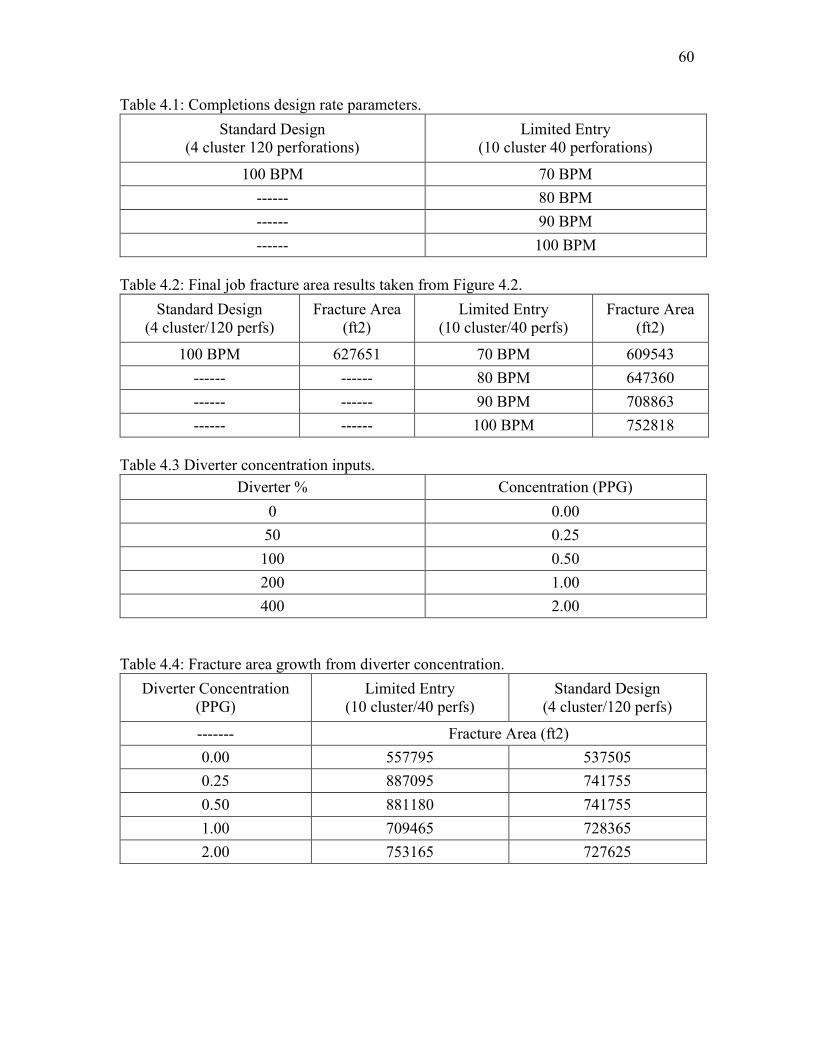
around the 100BPM rates were run (Table 4.1).
Each simulation was separately ran using the same fracture model. Figure 4.1 posts
graphical results of each injection rate. Table 4.2 lists the final job fracture areas from
Figure 4.2. The comparison between the 100 BPM limited entry and standard pump
schedule is noticeable. There is approximate a 17% increase in fracture growth with the
new design. The standard plan is achieving the same output as a ~75 BPM limited entry
design.
4.2 Diverter results
Limited entry results showed an improvement to fracture area growth. However,
simulations were performed without stopping and reinitiating the process. The workflow
plan is to understand rate affects before varying diversion.
The same pump schedule from the completions comparison is used. Rates were
fixed at 100 BPM. The diverter (proppant input in the simulator) ranged from 8-14 mesh
size. Diverter inputs were varied based on concentration percentage. Table 4.3 outlines the
percentages and corresponding concentrations. A 100% concentration correlates to the
real-time fracture job.
Fracture area growth based on diversion requires manipulation by the user. Hence,
graphical reports are not possible due to constantly terminating and resuming simulations.
However, numerical values were saved from the eliminate fractures and were summarized
with the final output of the simulation. Table 4.4 lists the results between the limited entry

54
and standard design at 100BPM based on diverter concentration variations.
A diverter concentration of 0% represents a clean fluid injection. Results indicate
that diverter is having an adverse effect on fracture area growth. However, increasing
diverter is not inflicting more fracture growth. Results between both completions cases
suggest an optimized volume of diverter to fracture area growth relation.
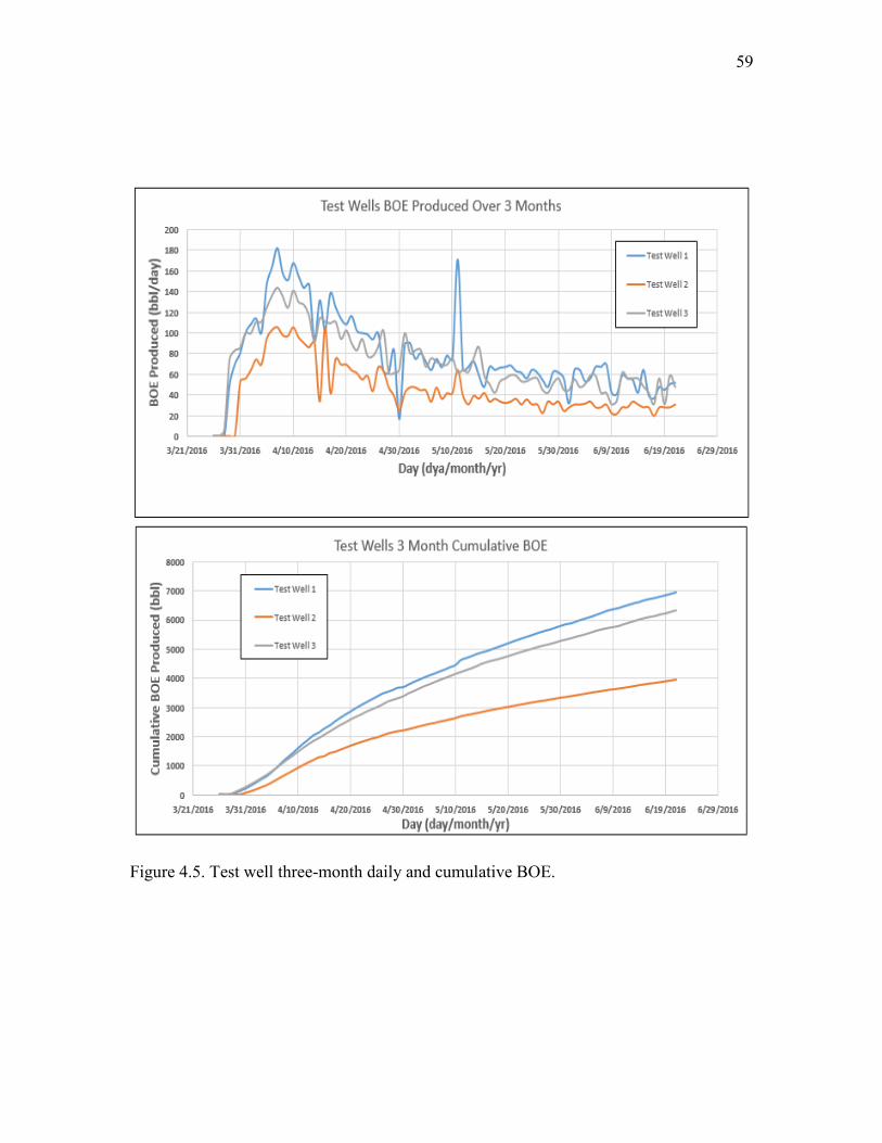
4.3 Well production comparison
Final model validations focus on well production data. Production has been online
for three months and been provided by the operator. Figures 4.2-4.5 show the daily and
cumulative gas, oil, water, and barrels of equivalent oil (BOE). For reference, the test well
completions are as follows:
Test Well 1 – Limited entry design
Test Well 2 – Standard completions design
Test Well 3 – Standard completions design
The overall pay thicknesses of each well is in the following:
Test Well 1 – 1919ft
Test Well 2 – 205ft
Test Well 3 – 1545ft
Test well 1 and 3 had the closest payzone thicknesses and were used for completions
comparisons. The limited entry well shows similar three-month cumulative production
results compared to the standard design. A noted difference is test well 1 produced
approximately 20% less water over the three-month period.

55
Figure 4.1 Cluster design post fracture area results. The green line represents the standard design treatment results used in the real fracture job.

56
Figure 4.2. Test well three-month daily and cumulative gas production.

57
Figure 4.3. Test well three-month daily and cumulative oil production.

58
Figure 4.4. Test well three-month daily and cumulative water production.
59
Figure 4.5. Test well three-month daily and cumulative BOE.
60
Table 4.1: Completions design rate parameters. Standard Design
(4 cluster 120 perforations) Limited Entry
(10 cluster 40 perforations)
100 BPM 70 BPM ------ 80 BPM ------ 90 BPM ------ 100 BPM
Table 4.2: Final job fracture area results taken from Figure 4.2.
Standard Design (4 cluster/120 perfs)
Fracture Area (ft2)
Limited Entry (10 cluster/40 perfs)
Fracture Area (ft2)
100 BPM 627651 70 BPM 609543 ------ ------ 80 BPM 647360 ------ ------ 90 BPM 708863 ------ ------ 100 BPM 752818
Table 4.3 Diverter concentration inputs.
Diverter % Concentration (PPG) 0 0.00 50 0.25 100 0.50 200 1.00 400 2.00
Table 4.4: Fracture area growth from diverter concentration. Diverter Concentration
(PPG) Limited Entry
(10 cluster/40 perfs) Standard Design
(4 cluster/120 perfs)
------- Fracture Area (ft2) 0.00 557795 537505 0.25 887095 741755 0.50 881180 741755 1.00 709465 728365 2.00 753165 727625

CHAPTER 5
CONCLUSIONS AND FUTURE RECOMMENDATIONS
There are multiple factors that dictate well performance. Each choice has a
significant influence on a well ranging from initial material costs and time required to
complete the well to the expected ultimate recovery. There are many challenges towards
accounting for the effects of natural fractures during hydraulic fracture stimulation. Natural
fractures can cause unanticipated stress shadowing affects, complex fluid and proppant
transport paths, and tortuous fracture paths. The demand for drilling in unconventional
formations containing complex fracture systems is increasing. Potential solutions, such as
limited entry design and diversion techniques, exist, but require optimization. It is
important that accurate numerical solutions pertaining to diverter and completions design
be incorporated into complex fracture modeling platforms that can accurately predict the
outputs of real-time treatment plans.
5.1 Cluster and diverter analysis conclusions
It is concluded that the limited entry completions design for the test wells is
feasible. The location of the clusters and perforations are strategically placed in stress zones
that will cause higher fracture area growth and production. The limited entry test wells
reported a 17% increase in fracture area. This area increase is likely due to reducing the

62
amount of inefficient perforations.
The use of diverter is common. However, no industry numerical modeling tool
simulates the effects of diverter placement propagated natural fractures. User manipulation
of the fracture sets, along with the combined use of Mangrove and FracMan, was required
in developing a valid diversion solution. Simulations in this study analyzed the effects of
various diverter concentrations. Final fracture area results yielded a 58% increase in
fracture area growth between the clean concentration (0 PPG) and actual pump schedule
concentration (0.5 PPG). There was no observable gain when increasing the concentration
past a certain extent.
The key to validating the effects of diversion and limited entry is the production
results. The three-month cumulative production from the limited entry well had similar
BOE results compared to the standard completions design. No clear increase in
performance can be due to multiple factors:
Porosity in this reservoir is difficult to define. It is dictated by drilling penetration
rate, torque on the mud motor (standpipe pressure), cuttings (percentage
limestone), gas shows, and fluorescence. These are all subjectively integrated to
establish pay and non-pay intervals in the lateral.
Porosity in this reservoir is laterally very discontinuous. That is to say that even
though the lateral may not encounter porosity at the same location, oil filled porosity
looming 10’ away from the well bore that can be reached with a completion.
There exist multiple degrees of freedom in the system. Each parameter affects
reservoir quality and their impacts can vary greatly between each well.

63
However, the limited entry design still shows value. Water production from the
limited entry well was 20% less over three months. These results were achieved by
reducing the perforation density by two-thirds. performance may be due to the fracture
network generated. Large half-length hydraulic fractures are produced when one
perforation receives majority of fluid. Large half-length hydraulic fractures not only
invade the drainage radius of nearby wells, but also fail to utilize the localized natural
fracture network near the wellbore. Consequently, single large hydraulic fractures create
three problems: the 1) production is limited and originates from limited amount of
perforations, 2) water volumes are decreased in poor payzones and lead to poor natural
fracture propagation, and 3) nearby wells are drained faster.
5.2 Future well design recommendations
It is recommended that perspective operating company of the test wells consider
incorporating a process that accurately solves for geomechanical properties of a future
planned well. The completions design of the well has a heavy impact on production
performance best on the cases studied. Furthermore, a diversion modeling approach has
been developed by manipulating the capabilities of FracMan and Mangrove. It is
recommended that collaboration be conducted with the two parties for developing and
integrating a standard diverter analysis option. The parameters simulated can be used by
drilling and completions engineers to further improve field production and possibly reduce
the capital costs of a well by evaluating the possibilities of: 1) using ultra high mesh diverter
to access smaller width fractures, 2) strategically placing the clusters and perforations into
the ideal stress zones, and 3) simulating future wells with FMI data to further calibrate the

64
limited entry and diverter model. More simulations under similar design criteria will
ultimately help engineers select design criteria that will optimize the performance of newly
drilled wells.
5.3 Thesis contributions to the scientific community
The material provided in this thesis has shown that it is possible to use Mangrove
and FracMan to develop a reasonable discrete fracture network model that can simulate
fracture changes under specific completions and diverter conditions. These numerical
packages allow a representative rendition of in-situ natural fractures and provide a basic
method for simulating injection. The modeling of the test wells serves as a benchmark for
simulating more complex problems, such as fracture effects on nearby wells, lithology
changes, and faults. It is important to note that variations in any of the spatially-local input
values used could have led to changes in the modeled system. This project has succeeded
in providing a proof-of-concept that FracMan and Mangrove can be used as a platform for
understanding injection into natural fractures. It can serve as 1) a staging point towards
developing other model simulations with an eventual increase in complexity, 2) a bridge
in solving completions and diversion questions associated with the natural fractures and
hydraulic fracture systems, and 3) be used for accurate production forecasting.

APPENDIX A
STACKED HEIGHT GROWTH EQUATION WIDTH SOLUTION
Nstack
j
H
H
jcpjfjcp
j
j
daaz
ah
ahz
aahgPE
zhw1
1,,,
1||
2
cosh)()(4),(
(2.9)
3214
IIIE
Nstack
j
H
H
jcpjfjcp
j
j
daaz
ah
ahz
aahgPI1
1,,,1
1||
2
cosh)()( (i)
2,11,11 III
(ii)
Nstack
j
H
H
jcpjfjcp
j
j
daaz
ah
ahz
hgPI1
1,,,1,1
1||
2
cosh)( (iii)
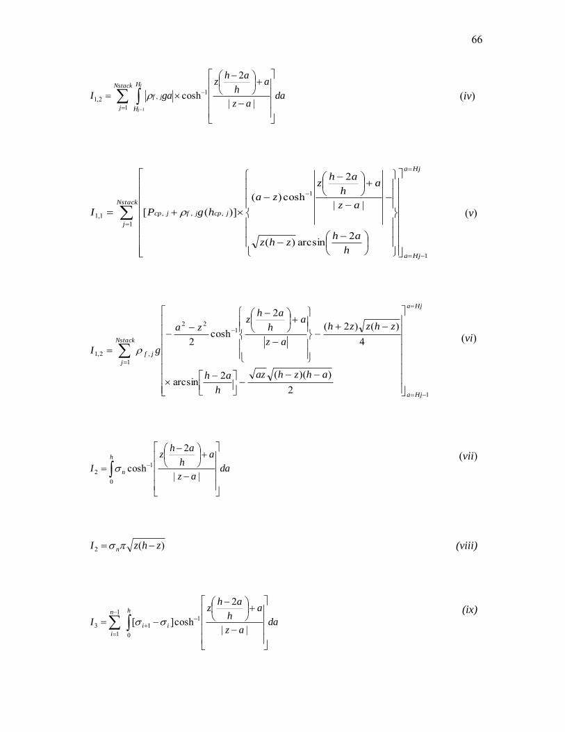
66
Nstack
j
H
H
jf
j
j
daaz
ah
ahz
gaI1
1,2,1
1||
2
cosh (iv)
Hja
Hja
Nstack
j
jcpjfjcp
h
ahzhz
az
ah
ahz
za
hgPI
1
1
1
,,,1,1
2arcsin)(
||
2
cosh)()]([ (v)
Hja
Hja
Nstack
j
jf
ahzhaz
h
ah
zhzzh
az
ah
ahz
za
gI
1
1
122
,2,1
2))((2arcsin
4)()2(
2
cosh2
(vi)
h
n daaz
ah
ahz
I
0
12 ||
2
cosh (vii)
)(2 zhzI n (viii)
h
ii
n
i
daaz
ah
ahz
I
0
11
1
13 ||
2
cosh][ (ix)

67
h
hharzhz
az
ah
ahz
I in
i
ii
2cos)(||
2
cosh][1
1
113
(x)
σn ........................................................... In-situ stress at the top of the fracture tip,
σi ................................................................................. In-situ stress at the i-th layer

APPENDIX B
STACKED HEIGHT GROWTH EQUATION HEIGHT SOLUTION
2.9a. Stress Intensity factor above the fracture
Nstack
j
H
H
jcpjfjcpIup
j
j
daah
aaahgP
hK
1
,,,
1
)()(2
(2.11a)
}{23
121 III
h
Nstack
j
2,11,11 III (a.i)
Nstack
j
H
H
jcpjfjcp
j
j
daah
aghPI
1
,,,1,11
(a.ii)
Nstack
j
H
H
jf
j
j
daah
agaI
1
,2,11
(a.iii)

69
Hja
Hja
Nstack
j
H
H
jcpjfjcp
ah
ahahaghPI
j
j
11
,,,1,1 arctan)(1
(a.iv)
Hja
Hja
Nstack
j
H
H
jf
j
jh
ahhaha
hagI
11
2
,2,11
2arcsin8
3)(4
32
(a.v)
h
n daah
aI
02 (a.vi)
22h
I n
(a.vii)
1
1 013
n
i
h
ii daah
aI
i (a.viii)
iii
n
i
ii hhhh
hhar
hI
i(2cos
2
1
113 (a.ix)
2.9b. Stress Intensity factor below the fracture
Nstack
j
H
H
jcpjfjcpIdown
j
j
daah
aaahgP
hK
1
,,,
1
)()(2
(2.11b)
2,11,11 III (b.i)
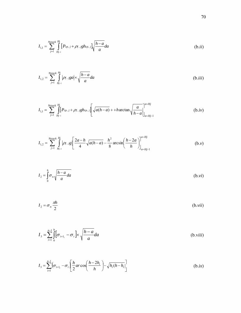
70
Nstack
j
H
H
jcpjfjcp
j
j
daa
ahghPI
1
,,,1,11
(b.ii)
Nstack
j
H
H
jf
j
j
daa
ahgaI
1
,2,11
(b.iii)
Hja
Hja
Nstack
j
H
H
jcpjfjcp
ah
ahahaghPI
j
j
11
,,,1,1 arctan)(1
(b.iv)
Hja
Hja
Nstack
j
H
H
jf
j
jh
ahhaha
hagI
11
2
,2,11
2arcsin8
)(4
2 (b.v)
h
n daa
ahI
02 (b.vi)
22h
I n
(b.vii)
1
1 013
n
i
h
ii daa
ahI
i (b.viii)
iii
n
i
ii hhhh
hhar
hI
i(2cos
2
1
113
(b.ix)
REFERENCES
[1] Barree, R. D. Economic Optimization of Horizontal-Well Completions in Unconventional Reservoirs. Society of Petroleum Engineers SPE 168612, 2015. [2] Wan, Jihn. Coupled Well and Reservoir Simulation Models to Optimize Completions Design and Operations for Subsurface Control. Society of Petroleum Engineers SPE 113635, 9 June 2008. [3] Cohen, Charles E. Parametric Study on Completion Design in Shale Reservoirs Based on Fracturing-to-Production Simulations. International Petroleum Technology Conference IPTC 17462, 2014. [4] Weng, Xiaowei. Modeling of Hydraulic-Fracture-Network Propagation in a Naturally Fractured Formation. Society of Petroleum Engineers SPE 140253, Nov. 2011. [5] Kreese, O., C. Cohen, and X. Weng. Numerical Modeling of Hydraulic Fracturing in Naturally Fractured Formations. American Rock Mechanics Association 11-363, 2011. [6] Cravero, M., and S. Ponti. D Simulation and Aggregation of Fracture Network. American Rock Mechanics Association 07-019, May 2007. [7] Mullen, J., Lowry, J.C., and Nwabuoku, K.C. 2010. Lessons Learned Developing the Eagle Ford Shale. Paper SPE 138446 presented at the SPE Tight Gas Conference, San Antonio, Texas, 2‒3 November. http://dx.doi.org/10.2118/138446-MS. [8] Cipolla, C., Mack, M., and Maxwell, S. 2010b. Reducing Exploration and Appraisal Risk in Low Permeability Reservoirs Using Microseismic Fracture Mapping - Part 2. SPE 138103 presented at the SPE Latin American & Caribbean Petroleum Engineering Conference held in Lima, Peru, 1–3 December 2010 [9] Shin, D. and Sharma, M. 2014. Factors Controlling the Simultaneous Propagation of Multiple Competing Fractures in a Horizontal Well. Paper SPE 168599 presented at the SPE Hydraulic Fracturing Technology Conference, The Woodlands, Texas, 4‒6 February. http://dx.doi.org/10.2118/168599-MS. [10] Cheng, Y. 2012. Mechanical Interaction of Multiple Fractures—Exploring Impacts of the Selection of the Spacing/Number of Perforation Clusters on Horizontal Shale Gas Wells. SPE J. 17 (4): 992‒1001. Paper SPE 125769-PA.
72
[11] Walker K., Wutherich K. and Terry J. Engineered Perforation design improves Fracture Placement and Productivity in Horizontal Shale Gas Wells. Paper SPE 154582 presented at the SPE Americas Unconventional Resources Conference, 5-7 June 2012, Pittsburg, Pennsylvania, USA [12] Cipolla C., Weng X, Malpani, R., and Luo, F. 2010 Shale Gas Production Decline Trend Over Time and Basins. Paper SPE 135555 presented at SPE Annual Technical Conference and Exhibition, Florence, Italy, 19-22 September. [13] Ahmed, M., and Andrea Nino-Penaloza. Engineering Solid Particulate Diverter to Control Fracture Complexity: Experimental Study. Society of Petroleum Engineers SPE 179144-MS, May 2016. [14]. Allison, D., Curry, S., and Todd, B. 2011. Restimulation of Wells using Biodegradable Particulates as Temporary Diverting Agents. Paper CSUG/SPE 149221 presented at the Canadian Unconventional Resources Converence, Calgary, Alberta, Canada, 15-17 November. Dio: 10.2118/149221-MS [15] Fisher, M.L., B.M. Davidson, A.K. Goodwin, E.O. Fielder, W.S. Buckler, and N.P. Steinberger. 2002. Integrating Fracture Mapping Technologies to Optimize Stimulations in the Barnett Shale. Paper SPE 77441 presented at the 2002 SPE Annual Technical Conference and Exhibition, San Antonio, Texas, USA, September 29-October 2. [16] Daniels, J., G. Walters, J. Le Calvez, J. Lassek, and D. Bentley. 2007. Contacting More of the Barnett Shale Through an Integration of Real-Time Microseismic Monitoring, Petrophysics, and Hydraulic Fracture Design. Paper SPE 110562 presented at the 2007 SPE Annual Technical Conference and Exhibition, Anaheim, California, USA, October 12-14. [17] Xu, W., J.L. Calvez, and M. Thiercelin. 2009. Characterization of Hydraulically-Induced Fracture Network Using Treatment and Microseismic Data in a Tight-Gas Formation: A Goemechanical Approach, Paper SPE 125237 presented at the 2009 SPE Tight Gas Completions Conference, San Antonio, Texas, USA, 15-17 June. [18] Meyer, B.R. and L.W. Bazan. 2011. A Discrete Fracture Network Model for Hydraulically-Induced Fractures: Theory, Parametric and Case Studies, Paper SPE 140514 presented at the SPE Hydraulic Fracturing Conference and Exhibition, Woodlands, Texas, January 24-26. [19]Kresse, O., C. Cohen, and X. Weng. Numerical Modeling of Hydraulic Fracturing in Naturally Fractured Formations. American Rock Mechanics Association ARMA 11-363, 26-29 June 2011. [20] Renshaw, C.E. and D.D. Pollard. 1995. An Experimentally Verified Criterion for Propagation Across Unbounded Frictional Interfaces in Brittle, Linear Elastic Materials. Int. J. Rock Mech. Min. Sci. & Geomech. Abstre., 32: 237-249
73
[21] Perkins, T.K. and Kern, L.R. 1961. Widths of Hydraulic Fractures. J Pet Technol 13 (9): 937–949. SPE-89-PA. http://dx.doi.org/10.2118/89-PA. [22]. Mack, M.G. and N.R. Warpinski. 2000. Mechanics of Hydraulic Fracturing. Chapter 6, Reservori Stimulation, 3rd Ed. Eds. Economides, M.J. and Nolte, K.G. John Wiley & Sons. [23]. Gu, H., and X. Weng. Hydraulic Fracture Crossing Natural Fracture at Non-Orthogonal Angles, A Criterion, Its Validation and Applications. Society of Petroleum Engineers SPE 139984, 24 Jan. 2011. [24]. Jaeger, J.C., Cook, N.G.W., and Zimmerman, R.w. (2007) Fundamentals of Rock Mechanics, 4th ed., Blackwell Publishing, Malden, MA, U.S.A. [25]. Weng, X., Kresse, O., Cohen, C., and Wu, R., and Gu, H. (2011) Modeling of Hydraulic Fracture Network Propagation in a Naturally Fractured Formation, paper SPE 140253, to be presented at the SPE Hydraulic Fracturing Technology Conference, The Woodlands, Texas, Jan. 24-26. [26]. Crouch, S.L. and A.<. Starfield. 1983. Boundary Element Methods in Solif Mechanics, George Allen & Unwin Ltd, London. [27]. Olson, J.E. 2004. Predicting Fracture Swarms – the Influence of Subcritical Crack Growth and the Crack-Tip Process Zone on Joint Spacing in Rock. In The initiation, Propagation, and Arrest of Joints and Other Fractures, Geological Society of London Special Publication 231, eds. J.W. Cosgrove and T. Engelder:73-87. [28]. Daneshy, A. 1978. Numerical Solution of Sand Transport in Hydraulic Fracturing. J. Pet. Tech., January 1978 (SPE 5636): 132-140. [29]. Hossain, M. E., and A. A. Al-Mejed. Fundamentals of Sustainable Drilling E ngineering. Vol. 1. Hoboken: John Wiley & Sons, 2015. [30]. J. McLennan, R. Carden, D. Curry, and C. Stone. Underbalanced Drilling Manual. Chicago: Gas Research Institute, n.d. Print. GRI Reference No. GRI-97/0236. [31]. Economides, M., and K. Nolte. Reservoir Stimulation. Hoboken: John Wiley & Sons, 2000. [32]. Crain, E. R. Elastic Constants/Mechanical Properties. Crain’s Petrophysical Handbook, 1978-2016.
Related Documents