UNIVERSIDAD DE CANTABRIA E.T.S. DE INGENIEROS DE CAMINOS, CANALES Y PUERTOS Departamento de Ciencias y Técnicas del Agua y del Medio Ambiente TESIS DOCTORAL OPTIMIZACIÓN EXPERIMENTAL Y NUMÉRICA DE VERTIDOS HIPERSALINOS EN EL MEDIO MARINO Presentada por: PILAR PALOMAR HERRERO Dirigida por: ÍÑIGO J. LOSADA RODRÍGUEZ JAVIER LÓPEZ LARA Santander, Abril 2014

Welcome message from author
This document is posted to help you gain knowledge. Please leave a comment to let me know what you think about it! Share it to your friends and learn new things together.
Transcript
UNIVERSIDAD DE CANTABRIA
E.T.S. DE INGENIEROS DE CAMINOS, CANALES Y PUERTOS
Departamento de Ciencias y Técnicas del Agua y del Medio Ambiente
TESIS DOCTORAL
OPTIMIZACIÓN EXPERIMENTAL Y
NUMÉRICA DE VERTIDOS HIPERSALINOS
EN EL MEDIO MARINO
Presentada por: PILAR PALOMAR HERRERO Dirigida por: ÍÑIGO J. LOSADA RODRÍGUEZ
JAVIER LÓPEZ LARA
Santander, Abril 2014


Te repito que no hace el plan a la vida, sino que ésta se lo traza a sí misma,
viviendo. ¿Fijarse un camino? El espacio que recorrerás será tu camino; no te
hagas, como planeta en su órbita, siervo de una trayectoria… (Unamuno).


Agradecimientos

Agradecimientos (II)
Queremos agradecer al Ministerio de Alimentación, Agricultura y Medio Ambiente su
confianza por la adjudicación de los proyectos de Investigación del Plan Nacional de
I+D+i:
◦ MEDVSA (045/RN08/03.3): “Desarrollo e implementación de una
metodología para la reducción del impacto ambiental de los vertidos de
salmuera procedentes de desaladoras”.
◦ SALTY (BIA2011-29031-C02-01): “Análisis de los procesos físicos en
campo cercano y lejano para la optimización de vertidos hiperdensos de
salmuera”.
Gracias a la financiación recibida en estos proyectos ha sido posible el desarrollo de
esta Tesis.
Agradecemos también a los técnicos de la Subdirección de Evaluación de Impacto
Ambiental y a ACUAMED. S.A su interés y apoyo en las reuniones de presentación
de resultados realizadas en el marco del proyecto MEDVSA.

RESUMEN DE LA TESIS CONTENIDO INTRODUCCIÓN Y MOTIVACIÓN .................................................................................................................... I
OBJETIVO Y METODOLOGÍA ......................................................................................................................... V
ANÁLISIS Y VALIDACIÓN DE LOS MODELOS COMERCIALES ........................................................................ VII
APLICACIÓN DE TÉCNICAS DE ANEMOMETRÍA LÁSER AL ESTUDIO EXPERIMENTAL DE VERTIDOS DE SALMUERA ................................................................................................................................................. XV
CARACTERIZACIÓN DEL COMPORTAMIENTO DEL CHORRO EN BASE AL ANÁLISIS DE DATOS EXPERIMENTALES ................................................................................................................................... XXVI
CARACTERIZACIÓN DE LA CAPA DE ESPARCIMIENTO LATERAL EN BASE AL ANÁLISIS DE LOS DATOS EXPERIMENTALES .................................................................................................................................. XXXV
NUEVOS MODELOS “BRIHNE” PARA LA SIMULACIÓN DE VERTIDOS DE SALMUERA ................................ XLI
DESARROLLO DE UNA GUÍA METODOLÓGICA PARA EL DISEÑO DE LOS VERTIDOS DE SALMUERA ....... XLVI
CONCLUSIONES Y CONTRIBUCIONES ......................................................................................................... LII
FUTURAS LÍNEAS DE INVESTIGACIÓN ........................................................................................................ LIV
Lista de Tablas ............................................................................................................................................ LV
Lista de Figuras .......................................................................................................................................... LVI

RESUMEN DE LA TESIS I
INTRODUCCIÓN Y MOTIVACIÓN
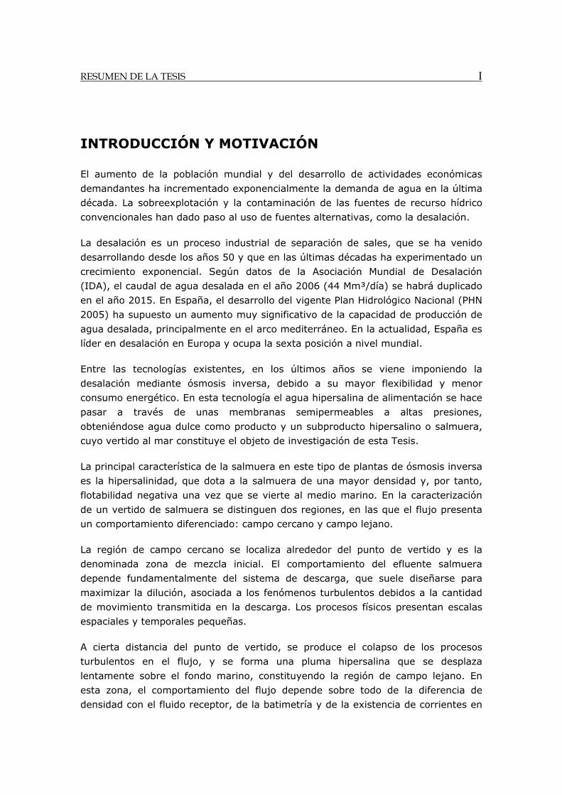
El aumento de la población mundial y del desarrollo de actividades económicas
demandantes ha incrementado exponencialmente la demanda de agua en la última
década. La sobreexplotación y la contaminación de las fuentes de recurso hídrico
convencionales han dado paso al uso de fuentes alternativas, como la desalación.
La desalación es un proceso industrial de separación de sales, que se ha venido
desarrollando desde los años 50 y que en las últimas décadas ha experimentado un
crecimiento exponencial. Según datos de la Asociación Mundial de Desalación
(IDA), el caudal de agua desalada en el año 2006 (44 Mm³/día) se habrá duplicado
en el año 2015. En España, el desarrollo del vigente Plan Hidrológico Nacional (PHN
2005) ha supuesto un aumento muy significativo de la capacidad de producción de
agua desalada, principalmente en el arco mediterráneo. En la actualidad, España es
líder en desalación en Europa y ocupa la sexta posición a nivel mundial.
Entre las tecnologías existentes, en los últimos años se viene imponiendo la
desalación mediante ósmosis inversa, debido a su mayor flexibilidad y menor
consumo energético. En esta tecnología el agua hipersalina de alimentación se hace
pasar a través de unas membranas semipermeables a altas presiones,
obteniéndose agua dulce como producto y un subproducto hipersalino o salmuera,
cuyo vertido al mar constituye el objeto de investigación de esta Tesis.
La principal característica de la salmuera en este tipo de plantas de ósmosis inversa
es la hipersalinidad, que dota a la salmuera de una mayor densidad y, por tanto,
flotabilidad negativa una vez que se vierte al medio marino. En la caracterización
de un vertido de salmuera se distinguen dos regiones, en las que el flujo presenta
un comportamiento diferenciado: campo cercano y campo lejano.
La región de campo cercano se localiza alrededor del punto de vertido y es la
denominada zona de mezcla inicial. El comportamiento del efluente salmuera
depende fundamentalmente del sistema de descarga, que suele diseñarse para
maximizar la dilución, asociada a los fenómenos turbulentos debidos a la cantidad
de movimiento transmitida en la descarga. Los procesos físicos presentan escalas
espaciales y temporales pequeñas.
A cierta distancia del punto de vertido, se produce el colapso de los procesos
turbulentos en el flujo, y se forma una pluma hipersalina que se desplaza
lentamente sobre el fondo marino, constituyendo la región de campo lejano. En
esta zona, el comportamiento del flujo depende sobre todo de la diferencia de
densidad con el fluido receptor, de la batimetría y de la existencia de corrientes en
II RESUMEN DE LA TESIS
el fondo marino. Los procesos físicos se producen a escalas más grandes, por lo
que la pluma puede desplazarse largas distancias sin apena dilución.
Respecto a los sistemas de vertido al mar de la salmuera, existen configuraciones
muy variadas, que se venían utilizando principalmente antes de que este tipo de
vertidos constituyesen una preocupación medioambiental. Algunos ejemplos son:
vertido directo superficial, vertido desde acantilado, sobre estructuras porosas, etc.
Sin embargo, en la actualidad, por su mayor eficacia en cuanto a dilución, se
imponen los vertidos mediante emisarios submarinos de chorros sumergidos.
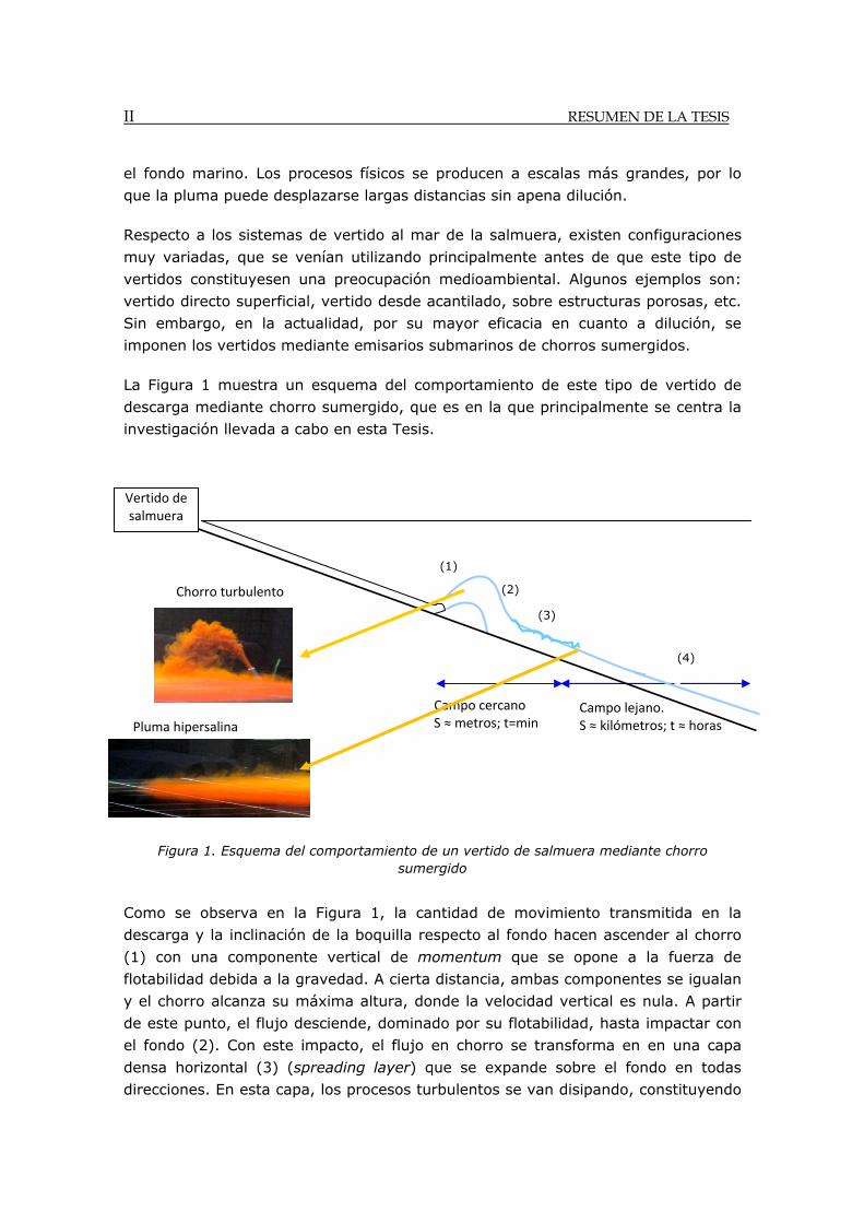
La Figura 1 muestra un esquema del comportamiento de este tipo de vertido de
descarga mediante chorro sumergido, que es en la que principalmente se centra la
investigación llevada a cabo en esta Tesis.
Figura 1. Esquema del comportamiento de un vertido de salmuera mediante chorro sumergido
Como se observa en la Figura 1, la cantidad de movimiento transmitida en la
descarga y la inclinación de la boquilla respecto al fondo hacen ascender al chorro
(1) con una componente vertical de momentum que se opone a la fuerza de
flotabilidad debida a la gravedad. A cierta distancia, ambas componentes se igualan
y el chorro alcanza su máxima altura, donde la velocidad vertical es nula. A partir
de este punto, el flujo desciende, dominado por su flotabilidad, hasta impactar con
el fondo (2). Con este impacto, el flujo en chorro se transforma en en una capa
densa horizontal (3) (spreading layer) que se expande sobre el fondo en todas
direcciones. En esta capa, los procesos turbulentos se van disipando, constituyendo
Pluma hipersalina
Chorro turbulento
(1)
(2)
(3)
Campo cercanoS ≈ metros; t=min
Campo lejano. S ≈ kilómetros; t ≈ horas
Vertido de salmuera
(4)
RESUMEN DE LA TESIS III
la transición desde el campo cercano al campo lejano, donde finalmente el flujo
forma una pluma hipersalina (4), que se desplaza lentamente sobre el fondo
marino.
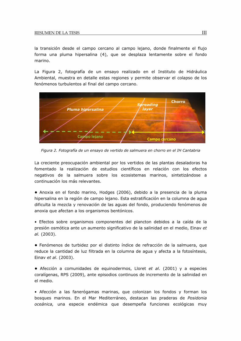
La Figura 2, fotografía de un ensayo realizado en el Instituto de Hidráulica
Ambiental, muestra en detalle estas regiones y permite observar el colapso de los
fenómenos turbulentos al final del campo cercano.
Figura 2. Fotografía de un ensayo de vertido de salmuera en chorro en el IH Cantabria
La creciente preocupación ambiental por los vertidos de las plantas desaladoras ha
fomentado la realización de estudios científicos en relación con los efectos
negativos de la salmuera sobre los ecosistemas marinos, sintetizándose a
continuación los más relevantes.
• Anoxia en el fondo marino, Hodges (2006), debido a la presencia de la pluma
hipersalina en la región de campo lejano. Esta estratificación en la columna de agua
dificulta la mezcla y renovación de las aguas del fondo, produciendo fenómenos de
anoxia que afectan a los organismos bentónicos.
• Efectos sobre organismos componentes del plancton debidos a la caída de la
presión osmótica ante un aumento significativo de la salinidad en el medio, Einav et
al. (2003).
• Fenómenos de turbidez por el distinto índice de refracción de la salmuera, que
reduce la cantidad de luz filtrada en la columna de agua y afecta a la fotosíntesis,
Einav et al. (2003).
• Afección a comunidades de equinodermos, Lloret et al. (2001) y a especies
coralígenas, RPS (2009), ante episodios continuos de incremento de la salinidad en
el medio.
• Afección a las fanerógamas marinas, que colonizan los fondos y forman los
bosques marinos. En el Mar Mediterráneo, destacan las praderas de Posidonia
oceánica, una especie endémica que desempeña funciones ecológicas muy
Campo cercano Campo lejano
Chorro Spreading
layer Pluma hipersalina
IV RESUMEN DE LA TESIS
importantes y que presenta un crecimiento muy lento y una alta sensibilidad a
modificaciones en las condiciones de su hábitat. La Posidonia oceanica está
protegida por la Directiva 92/43/CEE como hábitat de interés comunitario
prioritario. Para valorar el potencial efecto de los vertidos de salmuera sobre esta
especie, se llevó a cabo una investigación en España, Sanchez-Lizaso et al. (2008),
mediante ensayos en laboratorio y campo. Ante incrementos continuados del nivel
de salinidad, se observó la aparición de necrosis, caída de hojas y un aumento de la
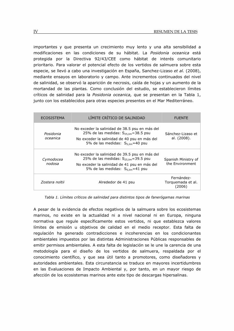
mortandad de las plantas. Como conclusión del estudio, se establecieron límites
críticos de salinidad para la Posidonia oceanica, que se presentan en la Tabla 1,
junto con los establecidos para otras especies presentes en el Mar Mediterráneo.
Tabla 1. Límites críticos de salinidad para distintos tipos de fanerógamas marinas
A pesar de la evidencia de efectos negativos de la salmuera sobre los ecosistemas
marinos, no existe en la actualidad ni a nivel nacional ni en Europa, ninguna
normativa que regule específicamente estos vertidos, ni que establezca valores
límites de emisión u objetivos de calidad en el medio receptor. Esta falta de
regulación ha generado contradicciones e incoherencias en los condicionantes
ambientales impuestos por las distintas Administraciones Públicas responsables de
emitir permisos ambientales. A esta falta de legislación se le une la carencia de una
metodología para el diseño de los vertidos de salmuera, respaldada por el
conocimiento científico, y que sea útil tanto a promotores, como diseñadores y
autoridades ambientales. Esta circunstancia se traduce en mayores incertidumbres
en las Evaluaciones de Impacto Ambiental y, por tanto, en un mayor riesgo de
afección de los ecosistemas marinos ante este tipo de descargas hipersalinas.
ECOSISTEMA LÍMITE CRÍTICO DE SALINIDAD FUENTE
Posidonia oceanica
No exceder la salinidad de 38.5 psu en más del 25% de las medidas: S25,lim=38.5 psu
No exceder la salinidad de 40 psu en más del 5% de las medidas: S5,lim=40 psu
Sánchez-Lizaso et al. (2008).
Cymodocea nodosa
No exceder la salinidad de 39.5 psu en más del 25% de las medidas: S25,lim=39.5 psu
No exceder la salinidad de 41 psu en más del 5% de las medidas: S5,lim=41 psu
Spanish Ministry of the Environment
Zostera noltii Alrededor de 41 psu Fernández-
Torquemada et al. (2006)
RESUMEN DE LA TESIS V
OBJETIVO Y METODOLOGÍA
Frente a esta situación, se ha planteado como principal objetivo de esta Tesis el
desarrollo de una metodología para el diseño de los vertidos al mar de salmuera,
bajo la perspectiva de minimizar su potencial impacto sobre el medio marino. Para
ello, el primer paso ha sido realizar una exhaustiva revisión del estado del arte de
todos aquellos aspectos que deben ser considerados en dicha metodología
(tecnologías de desalación, sistema de descarga, propiedades y comportamiento de
la salmuera, simulación del vertido, normativa, caracterización del clima,
ecosistemas sensibles, etc.). Durante esta revisión, han ido identificándose vacíos
de conocimiento científico en cada uno de estos temas, que requieren de nuevas
investigaciones.
Entre los vacíos identificados, se han seleccionado aquellos relacionados con el
comportamiento de este tipo de vertidos de flotabilidad negativa y con su
predicción mediante modelos numéricos. Seleccionados estos vacíos, se han
planteado los siguientes objetivos parciales que, junto con el desarrollo de la Guía
metodológica, conforman la meta planteada en la esta Tesis.
Analizar desde una perspectiva crítica y validar con datos experimentales las
herramientas comerciales más utilizadas para simular el comportamiento de los
vertidos al mar de salmuera. Determinar su grado de fiabilidad.
Estudiar el comportamiento de este tipo de flujos, profundizando en los procesos
hidrodinámicos y de mezcla y contrastando las hipótesis simplificativas asumidas en
las aproximaciones numéricas.
Generar una base de datos experimentales de suficiente calidad y resolución para
calibrar y validar modelos numéricos.
Desarrollar herramientas de modelado de vertidos de salmuera alternativas a las
comerciales, superando sus limitaciones y con un mejor ajuste a los datos
experimentales.
Centrándonos principalmente en plantas desaladoras de osmosis inversa y
descargas mediante chorros sumergidos, se presenta a continuación un esquema
de la metodología de trabajo llevada a cabo en la Tesis. Esta metodología
constituye una secuencia ordenada de los pasos para alcanzar los objetivos
planteados.
VI RESUMEN DE LA TESIS
1. Revisión de Estudios de Impacto Ambiental (EsIA), Declaraciones de Impacto
Ambiental (DIAs) y Autorizaciones de Vertido (AAVV) de vertidos de plantas
desaladoras. Identificación de carencias generales a nivel nacional. Objetivo
de desarrollar una metodología de diseño para minimizar impactos.
2. Establecimiento de los pasos metodológicos básicos para el diseño ambiental
del vertido de salmuera, determinando todos los aspectos a considerar.
3. Revisión del estado del arte en cada aspecto a considerar, identificación de
vacíos de conocimiento científico. Selección de “vacíos” relacionados con el
comportamiento del vertido de salmuera y su predicción numérica, para
realizar una investigación en el marco de la Tesis. En base a esta selección,
se establecen objetivos parciales, complementarios al desarrollo de la
metodología de diseño.
4. Para el análisis y validación de los modelos comerciales, se han estudiado en
detalle sus manuales y se han ejecutado numerosos casos utilizando todas
las opciones disponibles y comparando resultados con datos experimentales.
5. Para estudiar el comportamiento de estos vertidos, se han diseñado y
ejecutado ensayos experimentales en el laboratorio del IH Cantabria. Para el
análisis de los datos, se han programado códigos específicos.
6. Para generar una base de datos experimentales de suficiente de calidad para
calibrar y validar modelos numéricos, se han utilizado técnicas ópticas
avanzadas de anemometría láser y alta resolución, para la ejecución de los
ensayos experimentales en el IH Cantabria.
7. Para desarrollar nuevas herramientas de modelado (“brIHne”), se han
analizado y seleccionado aproximaciones numéricas de publicaciones
científicas, se han recalibrado con datos experimentales, se han programado
códigos en Matlab y se han trasladado a un portal web de acceso a usuarios.
8. Para la elaboración de la Guía Metodológica, se analizaron proyectos de
plantas desaladoras y datos de plantas en funcionamiento.
RESUMEN DE LA TESIS VII
ANÁLISIS Y VALIDACIÓN DE LOS MODELOS COMERCIALES
De la revisión de Estudios de Impacto Ambiental y proyectos, se han identificado
los software CORMIX, Doneker et al. (2001), VISUAL PLUMES, Frick (2004) y
VISJET como los más utilizados para simular el comportamiento de vertidos al mar
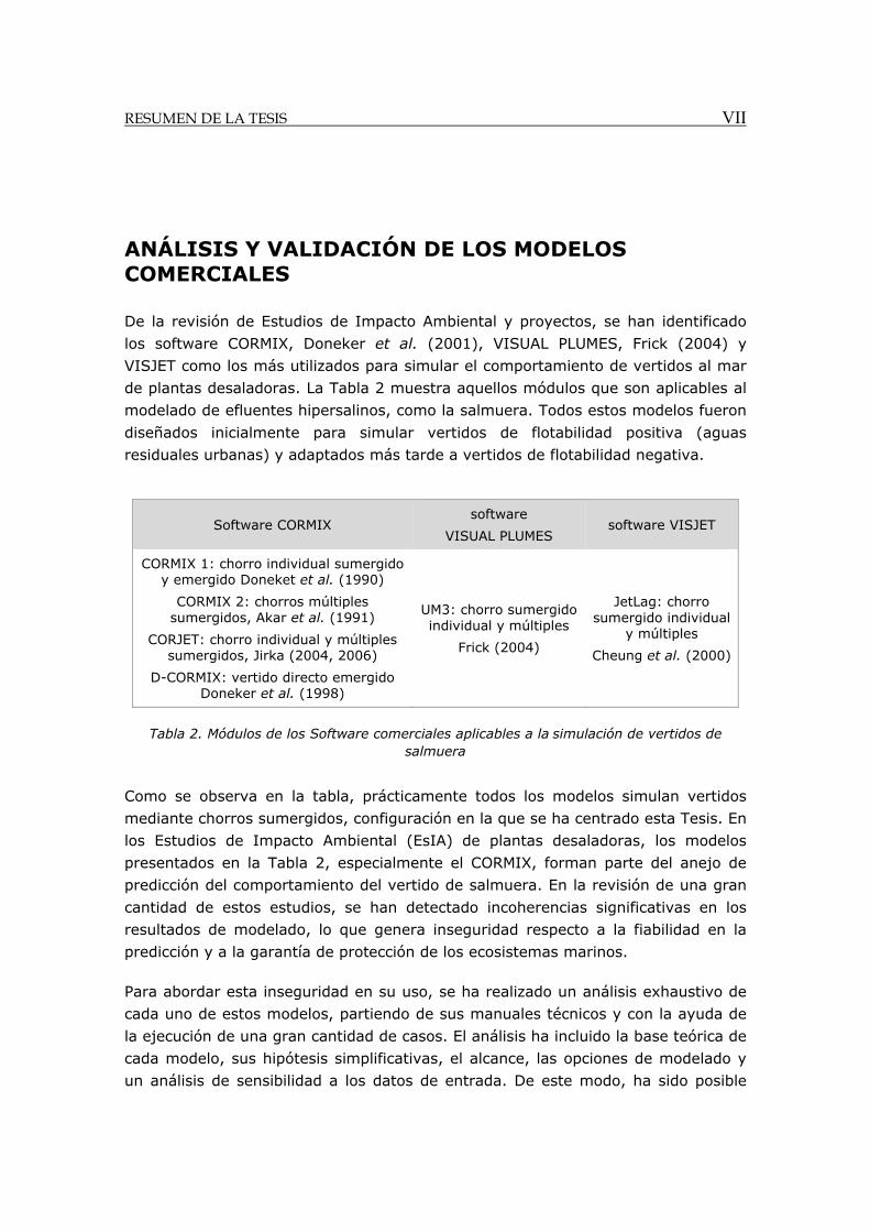
de plantas desaladoras. La Tabla 2 muestra aquellos módulos que son aplicables al
modelado de efluentes hipersalinos, como la salmuera. Todos estos modelos fueron
diseñados inicialmente para simular vertidos de flotabilidad positiva (aguas
residuales urbanas) y adaptados más tarde a vertidos de flotabilidad negativa.
Tabla 2. Módulos de los Software comerciales aplicables a la simulación de vertidos de salmuera
Como se observa en la tabla, prácticamente todos los modelos simulan vertidos
mediante chorros sumergidos, configuración en la que se ha centrado esta Tesis. En
los Estudios de Impacto Ambiental (EsIA) de plantas desaladoras, los modelos
presentados en la Tabla 2, especialmente el CORMIX, forman parte del anejo de
predicción del comportamiento del vertido de salmuera. En la revisión de una gran
cantidad de estos estudios, se han detectado incoherencias significativas en los
resultados de modelado, lo que genera inseguridad respecto a la fiabilidad en la
predicción y a la garantía de protección de los ecosistemas marinos.
Para abordar esta inseguridad en su uso, se ha realizado un análisis exhaustivo de
cada uno de estos modelos, partiendo de sus manuales técnicos y con la ayuda de
la ejecución de una gran cantidad de casos. El análisis ha incluido la base teórica de
cada modelo, sus hipótesis simplificativas, el alcance, las opciones de modelado y
un análisis de sensibilidad a los datos de entrada. De este modo, ha sido posible
Software CORMIX software
VISUAL PLUMES software VISJET
CORMIX 1: chorro individual sumergido y emergido Doneket et al. (1990)
CORMIX 2: chorros múltiples sumergidos, Akar et al. (1991)
CORJET: chorro individual y múltiples sumergidos, Jirka (2004, 2006)
D-CORMIX: vertido directo emergido Doneker et al. (1998)
UM3: chorro sumergido individual y múltiples
Frick (2004)
JetLag: chorro sumergido individual
y múltiples
Cheung et al. (2000)
VIII RESUMEN DE LA TESIS
identificar las capacidades y limitaciones reales de los modelos en contraste con las
teóricas establecidas en sus manuales, así como comprender las ventajas e
inconvenientes de cada tipo de aproximación numérica para este tipo de flujos.
Dado que una carencia común a todos estos modelos es la falta de datos de
validación de sus autores para descargas de efluentes de flotabilidad negativa, se
ha decidido llevar a cabo una validación de dichos modelos, comparando sus
resultados con datos experimentales publicados. La mayor parte de los estudios
experimentales disponibles para vertidos de chorros densos se centran en
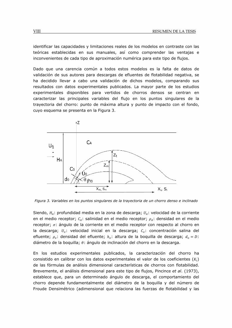
caracterizar las principales variables del flujo en los puntos singulares de la
trayectoria del chorro: punto de máxima altura y punto de impacto con el fondo,
cuyo esquema se presenta en la Figura 3.
Figura 3. Variables en los puntos singulares de la trayectoria de un chorro denso e inclinado
Siendo, : profundidad media en la zona de descarga; : velocidad de la corriente
en el medio receptor; : salinidad en el medio receptor; : densidad en el medio
receptor; : ángulo de la corriente en el medio receptor con respecto al chorro en
la descarga; : velocidad inicial en la descarga; : concentración salina del
efluente; : densidad del efluente; : altura de la boquilla de descarga; :
diámetro de la boquilla; : ángulo de inclinación del chorro en la descarga.
En los estudios experimentales publicados, la caracterización del chorro ha
consistido en calibrar con los datos experimentales el valor de los coeficientes ( )
de las fórmulas de análisis dimensional características de chorros con flotabilidad.
Brevemente, el análisis dimensional para este tipo de flujos, Pincince et al. (1973),
establece que, para un determinado ángulo de descarga, el comportamiento del
chorro depende fundamentalmente del diámetro de la boquilla y del número de
Froude Densimétrico (adimensional que relaciona las fuerzas de flotabilidad y las
Xi, Si Xm, Sm
Zt
Zm
RESUMEN DE LA TESIS IX
fuerzas de inercia en el flujo). La relación de dependencia es una constante. ,
para cada variable y punto de la trayectoria, que se calibra mediante datos
experimentales. A modo de ejemplo, se presentan las fórmulas de análisis
dimensional para algunas variables del chorro en un medio receptor en reposo.
; ; ; ; ; , . 1
Donde:
: máxima altura del borde superior del chorro.
: máxima altura del eje del chorro.
: posición horizontal del chorro en el punto de máxima altura.
: dilución en el eje en el punto de máxima altura.
: posición horizontal del chorro en el punto de impacto con el fondo.
: dilución en el eje en el punto de impacto con el fondo.
: coeficientes de análisis dimensional a obtener experimentalmente.
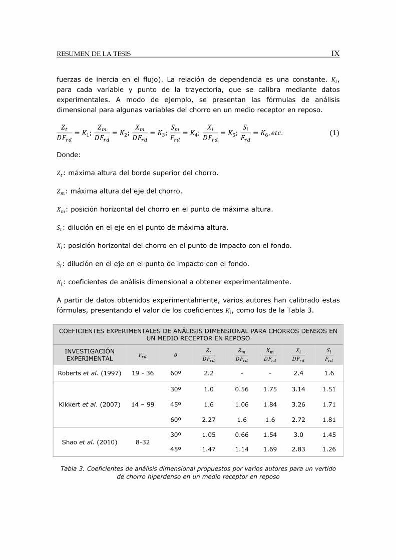
A partir de datos obtenidos experimentalmente, varios autores han calibrado estas
fórmulas, presentando el valor de los coeficientes , como los de la Tabla 3.
Tabla 3. Coeficientes de análisis dimensional propuestos por varios autores para un vertido de chorro hiperdenso en un medio receptor en reposo
COEFICIENTES EXPERIMENTALES DE ANÁLISIS DIMENSIONAL PARA CHORROS DENSOS EN UN MEDIO RECEPTOR EN REPOSO
INVESTIGACIÓN EXPERIMENTAL
Roberts et al. (1997) 19 - 36 60º 2.2 - - 2.4 1.6
Kikkert et al. (2007) 14 – 99
30º 1.0 0.56 1.75 3.14 1.51
45º 1.6 1.06 1.84 3.26 1.71
60º 2.27 1.6 1.6 2.72 1.81
Shao et al. (2010) 8-32 30º 1.05 0.66 1.54 3.0 1.45
45º 1.47 1.14 1.69 2.83 1.26
X RESUMEN DE LA TESIS
Recopilados los coeficientes experimentales publicados por diversos autores, la
validación de los modelos comerciales se ha realizado comparando estos
coeficientes con los equivalentes obtenidos de la simulación numérica con cada
modelo.
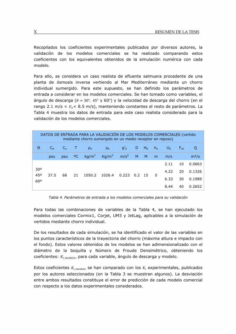
Para ello, se considera un caso realista de efluente salmuera procedente de una
planta de ósmosis inversa vertiendo al Mar Mediterráneo mediante un chorro
individual sumergido. Para este supuesto, se han definido los parámetros de
entrada a considerar en los modelos comerciales. Se han tomado como variables, el
ángulo de descarga ( 30°, 45° y 60°) y la velocidad de descarga del chorro (en el
rango 2.1 m/s < < 8.5 m/s), manteniendo constantes el resto de parámetros. La
Tabla 4 muestra los datos de entrada para este caso realista considerado para la
validación de los modelos comerciales.
Tabla 4. Parámetros de entrada a los modelos comerciales para su validación
Para todas las combinaciones de variables de la Tabla 4, se han ejecutado los
modelos comerciales Cormix1, Corjet, UM3 y JetLag, aplicables a la simulación de
vertidos mediante chorro individual.
De los resultados de cada simulación, se ha identificado el valor de las variables en
los puntos característicos de la trayectoria del chorro (máxima altura e impacto con
el fondo). Estos valores obtenidos de los modelos se han adimensionalizado con el
diámetro de la boquilla y Número de Froude Densimétrico, obteniendo los
coeficientes: _ , para cada variable, ángulo de descarga y modelo.
Estos coeficientes _ se han comparado con los experimentales, publicados
por los autores seleccionados (en la Tabla 3 se muestran algunos). La desviación
entre ambos resultados constituye el error de predicción de cada modelo comercial
con respecto a los datos experimentales considerados.
DATOS DE ENTRADA PARA LA VALIDACIÓN DE LOS MODELOS COMERCIALES (vertido mediante chorro sumergido en un medio receptor en reposo)
Θ CA Co T ρ0 ρA g’0 D HA ho U0 Frd Q
psu psu ºC kg/m3 Kg/m3 m/s2 M M m m/s m³/s
30º
45º
60º
37.5 68 21 1050.2 1026.4 0.223 0.2 15 0
2.11 10 0.0663
4.22 20 0.1326
6.33 30 0.1989
8.44 40 0.2652
RESUMEN DE LA TESIS XI
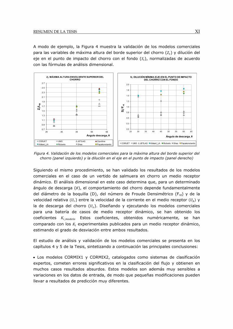
A modo de ejemplo, la Figura 4 muestra la validación de los modelos comerciales
para las variables de máxima altura del borde superior del chorro ( ) y dilución del
eje en el punto de impacto del chorro con el fondo ( ), normalizadas de acuerdo
con las fórmulas de análisis dimensional.
Figura 4. Validación de los modelos comerciales para la máxima altura del borde superior del chorro (panel izquierdo) y la dilución en el eje en el punto de impacto (panel derecho)
Siguiendo el mismo procedimiento, se han validado los resultados de los modelos
comerciales en el caso de un vertido de salmuera en chorro un medio receptor
dinámico. El análisis dimensional en este caso determina que, para un determinado
ángulo de descarga ( ), el comportamiento del chorro depende fundamentalmente
del diámetro de la boquilla (D), del número de Froude Densimétrico (Frd) y de la
velocidad relativa ) entre la velocidad de la corriente en el medio receptor y
la de descarga del chorro ( ). Diseñando y ejecutando los modelos comerciales
para una batería de casos de medio receptor dinámico, se han obtenido los
coeficientes _ Estos coeficientes, obtenidos numéricamente, se han
comparado con los experimentales publicados para un medio receptor dinámico,
estimando el grado de desviación entre ambos resultados.
El estudio de análisis y validación de los modelos comerciales se presenta en los
capítulos 4 y 5 de la Tesis, sintetizando a continuación las principales conclusiones:
Los modelos CORMIX1 y CORMIX2, catalogados como sistemas de clasificación
expertos, cometen errores significativos en la clasificación del flujo y obtienen en
muchos casos resultados absurdos. Estos modelos son además muy sensibles a
variaciones en los datos de entrada, de modo que pequeñas modificaciones pueden
llevar a resultados de predicción muy diferentes.
0.7
0.9
1.1
1.3
1.5
1.7
1.9
2.1
2.3
2.5
2.7
25 35 45 55 65
Zt/L
M
Ángulo descarga, θ
Zt: MÁXIMA ALTURA ENVOLVENTE SUPERIOR DEL CHORRO
CORJET UM3 JETLAG Cipollina
Kikkert_LA Roberts Shao Papakonstantis
0.0
0.3
0.5
0.8
1.0
1.3
1.5
1.8
2.0
25 30 35 40 45 50 55 60 65
Si/
Frd
Ángulo de descarga, θ
Si: DILUCIÓN MÍNIMA (EJE) EN EL PUNTO DE IMPACTO DEL CHORRO CON EL FONDO
CORJET UM3 JETLAG Kikkert_LA Roberts Shao Papakonstantis
XII RESUMEN DE LA TESIS
A pesar de que CORMIX2 en teoría simula diferentes configuraciones de tramo
difusor, todas al final se reducen a un difusor unidireccional y bidireccional con
boquillas perpendiculares al mismo. Además, para el caso de difusor bidireccional,
asume la simplificación de un vertido equivalente mediante chorro único vertical;
hipótesis que, si bien es aceptable en vertidos hipodensos, es del todo incorrecta en
vertidos hiperdensos, como la salmuera.
Los modelos CORJET, UM3 y JetLag, basados en la integración de las ecuaciones
diferenciales, son para este caso más fiables. Sin embargo, al asumir un medio
receptor ilimitado, su dominio de cálculo se reduce a la trayectoria del chorro antes
de impactar con el fondo. Sus hipótesis, que derivan tradicionalmente de estudios
con chorro neutros, requieren ser contrastadas para chorros de flotabilidad
negativa.
Por no simular efectos de re-intrusión o adherencia del flujo, se recomienda
limitar el uso de los modelos CORJET, UM3 y JETLAG al rango de inclinaciones: 15º 75º.
A pesar de la evidencia experimental, Roberts et al. (1987), de la influencia en la
dilución del efluente, del ángulo entre la corriente ambiental y el chorro, los
resultados de CORJET, UM3 y JETLAG son prácticamente insensibles a este
parámetro.
En la simulación de vertidos mediante tramo difusor de múltiples boquillas
unidireccionales con UM3 y CORJET, se asumen diferentes hipótesis para modelar la
interacción entre chorros contiguos. Sin embargo, ambos modelos se muestran
insensibles a la separación entre boquillas en el caso de chorros que interaccionan,
obteniendo los mismos resultados independientemente del valor de dicha
separación.
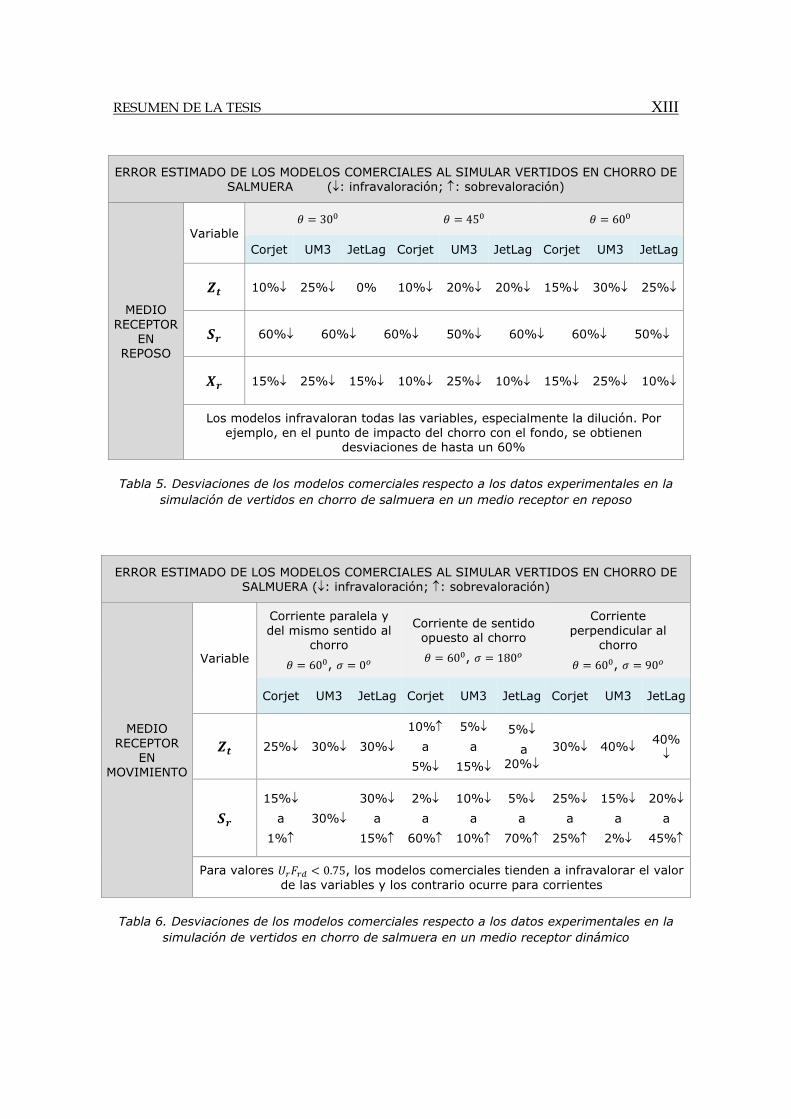
Como síntesis de la validación de los modelos comerciales, la Tabla 5 muestra las
desviaciones obtenidas entre los resultados numéricos y los datos experimentales
publicados para el caso de vertido en chorro de salmuera en un medio receptor en
reposo. La Tabla 6 presenta estas desviaciones para el vertido en un medio
receptor dinámico (con presencia de una corriente).
RESUMEN DE LA TESIS XIII
Tabla 5. Desviaciones de los modelos comerciales respecto a los datos experimentales en la simulación de vertidos en chorro de salmuera en un medio receptor en reposo
Tabla 6. Desviaciones de los modelos comerciales respecto a los datos experimentales en la simulación de vertidos en chorro de salmuera en un medio receptor dinámico
ERROR ESTIMADO DE LOS MODELOS COMERCIALES AL SIMULAR VERTIDOS EN CHORRO DE SALMUERA (: infravaloración; : sobrevaloración)
MEDIO RECEPTOR
EN REPOSO
Variable 30 45 60
Corjet UM3 JetLag Corjet UM3 JetLag Corjet UM3 JetLag
10% 25% 0% 10% 20% 20% 15% 30% 25%
60% 60% 60% 50% 60% 60% 50%
15% 25% 15% 10% 25% 10% 15% 25% 10%
Los modelos infravaloran todas las variables, especialmente la dilución. Por ejemplo, en el punto de impacto del chorro con el fondo, se obtienen
desviaciones de hasta un 60%
ERROR ESTIMADO DE LOS MODELOS COMERCIALES AL SIMULAR VERTIDOS EN CHORRO DE SALMUERA (: infravaloración; : sobrevaloración)
MEDIO RECEPTOR
EN MOVIMIENTO
Variable
Corriente paralela y del mismo sentido al
chorro
60 , 0
Corriente de sentido opuesto al chorro
60 , 180
Corriente perpendicular al
chorro
60 , 90
Corjet UM3 JetLag Corjet UM3 JetLag Corjet UM3 JetLag
25% 30% 30%
10%
a
5%
5%
a
15%
5%
a 20%
30% 40% 40%
15%
a
1%
30%
30%
a
15%
2%
a
60%
10%
a
10%
5%
a
70%
25%
a
25%
15%
a
2%
20%
a
45%
Para valores 0.75, los modelos comerciales tienden a infravalorar el valor de las variables y los contrario ocurre para corrientes
XIV RESUMEN DE LA TESIS
A la vista de los resultados de las Tablas 5 y 6, se establecen las siguientes
conclusiones:
CORJET, UM3 y JetLag infravaloran ligeramente las dimensiones y
significativamente el ratio de dilución del chorro para todos los casos de vertido en
un medio receptor en reposo.
Para un medio receptor en movimiento, los modelos comerciales siguen la
tendencia de aumentar la dilución con la velocidad de la corriente en el medio
receptor. Sin embargo, presentan desviaciones importantes respecto a los datos
experimentales en la simulación del efecto de la orientación de la corriente con
respecto al chorro. En particular:
CORJET y JetLag obtienen prácticamente los mismos valores de dilución
independientemente de la dirección de la corriente. Estos modelos presentan
para la dilución en el punto de impacto un buen ajuste con los datos
experimentales en el caso de corrientes con la misma dirección y sentido que
el chorro (coflowing). Sin embargo, cuando las corrientes son significativa
( 0.25), sobreestiman significativamente este parámetro en el caso de
corrientes perpendiculares (transverse) y de dirección opuesta al chorro
(counterflowing).
UM3 infraestima el valor de la dilución en el punto de impacto del chorro con
el fondo en el caso de corrientes de la misma dirección y sentido que el chorro
(coflowing). Sin embargo, presenta un buen ajuste en el caso de corrientes
perpendiculares (transverse) y de sentido opuesto (counterflowing) al chorro.
Como complemento al análisis y validación de los modelos comerciales, y en base a
la experiencia, se ha propuesto en la tesis una tabla de valores realistas y
recomendados para los parámetros de entrada del modelado. Esta tabla propone
valores óptimos en cuando al diseño del dispositivo de vertido de salmuera en
chorro (con el objetivo de maximizar la dilución del efluente), considerando
descargas al Mar Mediterráneo.
RESUMEN DE LA TESIS XV
APLICACIÓN DE TÉCNICAS DE ANEMOMETRÍA LÁSER AL ESTUDIO EXPERIMENTAL DE VERTIDOS DE SALMUERA
Introducción y configuración de los ensayos
El deficiente grado de ajuste de los resultados de los modelos comerciales a los
datos experimentales deja entrever que este tipo de chorros inclinados y con
flotabilidad negativa presentan un comportamiento complejo, que no puede ser
simulado correctamente con las aproximaciones numéricas clásicas de chorros
neutros. Por otra parte, los estudios disponibles en la bibliografía en relación con
este tipo de flujos no describen en detalle su comportamiento sino que se centran
en calibrar las fórmulas de análisis dimensional en los puntos característicos de la
trayectoria del chorro.
Para poner remedio a este desconocimiento, profundizar en los procesos
hidrodinámicos y de mezcla en el flujo, contrastar las hipótesis simplificativas
asumidas en las aproximaciones numéricas y generar una base de datos para la
calibración y validación de modelos numéricos, se ha realizado un estudio
experimental del campo cercano de vertidos en chorro de salmuera.
Los ensayos experimentales se han diseñado y ejecutado en el laboratorio del
Instituto de Hidráulica Ambiental, utilizando técnicas ópticas láser: PIV (Particle
Image Velocymetry) y PLIF (Planar Laser Induced Fluorescence). Frente a las
técnicas convencionales, la anemometría láser presenta las ventajas de ser no-
intrusiva y de medir simultáneamente los campos de velocidad (con PIV) y de
concentración (con PLIF) en el flujo, con una alta resolución espacial y temporal, lo
que permite una caracterización de detalle. Entre sus desventajas, está su
complejidad en la selección de los parámetros de ensayo y en su ejecución, la
sensibilidad de los equipos y la dificultad en el post-procesado, gestión y análisis de
los datos experimentales.
El estudio experimental se ha centrado en chorros de salmuera sumergidos vertidos
en un medio receptor en reposo. Como variables de diseño, se han considerado el
ángulo de descarga (15° 75°) y el número de Froude Densimétrico (10
35), estudiando su influencia en el comportamiento del vertido.
XVI RESUMEN DE LA TESIS
Tomando como prototipo un vertido de salmuera procedente de una planta de
ósmosis inversa, con tasa de conversión del 50%, descargando al Mar
Mediterráneo, las variables geométricas y cinemáticas se han escalado a 1:40
(escala adecuada teniendo en cuenta parámetros de modelado y la contaminación
del tanque). Para garantizar la semejanza dinámica, se ha mantenido, asumiendo
flujo turbulento completamente desarrollado, el valor del número de Froude
Densimétrico entre prototipo y ensayo.
Se han llevado a cabo dos grupos de experimentos. El primero, con un total de 15
ensayos, se ha enfocado a caracterizar el comportamiento en la región del chorro
de salmuera, mientras que con el segundo, de 9 ensayos, se ha caracterizado la
capa de esparcimiento lateral (spreading layer), que se forma tras el impacto del
chorro con el fondo. Esto ha hecho posible describir de forma pionera el
comportamiento de del flujo en toda la región de campo cercano.
Dado que no existen en la bibliografía descripciones detalladas sobre la aplicación
de técnicas ópticas a este tipo de vertidos en chorro hipersalinos, ha sido necesario
invertir un tiempo considerable en el aprendizaje de la técnica y su adaptación al
estudio experimental de este tipo de flujos.
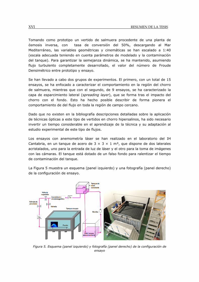
Los ensayos con anemometría láser se han realizado en el laboratorio del IH
Cantabria, en un tanque de acero de 3 × 3 × 1 m³, que dispone de dos laterales
acristalados, uno para la entrada de luz de láser y el otro para la toma de imágenes
con las cámaras. El tanque está dotado de un falso fondo para ralentizar el tiempo
de contaminación del tanque.
La Figura 5 muestra un esquema (panel izquierdo) y una fotografía (panel derecho)
de la configuración de ensayo.
Figura 5. Esquema (panel izquierdo) y fotografía (panel derecho) de la configuración de ensayo
RESUMEN DE LA TESIS XVII
El efluente, simulando la salmuera, se almacena en un tanque de plástico de 1000
litros, que se encuentra conectado y en continua recirculación con un depósito de
acero de 100 litros, situado a unos 4.5 m sobre el suelo. Desde este depósito, que
se mantiene a nivel constante, parte un tubo de plástico desde donde el efluente se
vierte por gravedad hacia el tanque de ensayo. En este último, se conecta con un
tubo de acero, que representa la boquilla de vertido. El caudal se controla de forma
continua con un caudalímetro electromagnético.
El tanque de ensayo se rellena de agua dulce, simulando el fluido receptor. El
efluente salmuera en el ensayo es una mezcla de agua dulce y sal común (NaCl), a
la que se añade un trazador fluorescente y pequeñas partículas de poliamida, para
las medidas de concentración y velocidad en el flujo, respectivamente.
Para la iluminación del flujo, se ha utilizado un láser Q-switched doble pulso Nd-
Yag, con una longitud de onda del haz de luz de 532 nm. El láser está dotado de un
brazo telescópico para desplazar el plano láser bidimensional con distinta
orientación con respecto al fondo del tanque. En los ensayos realizados, el brazo se
ha ajustado para crear un haz láser vertical que pase por el centro de la boquilla de
vertido.
Para la toma de imágenes PIV y PLIF, se han utilizado cámaras de tipo CCD
ImagerProX 4M LaVision, con resolución de 2048 × 2048 pixels, colocadas en
paralelo, perpendiculares al plano láser y a la misma distancia al objeto de
medición. Las imágenes captadas se transmiten a dos ordenadores para el
almacenamiento y post-procesado de los datos, proceso que ha limitado la
frecuencia de adquisición a 5 Hz en estos ensayos.
Aplicación de la Técnica PIV: medida de los campos de velocidades
La técnica PIV consiste en determinar simultáneamente dos componentes de la
velocidad instantánea en varios puntos de una sección bidimensional del flujo. Para
un tiempo , un plano del flujo sembrado de pequeñas partículas es iluminado por
el haz láser y la imagen de las manchas de difusión de las partículas se graba sobre
una cámara CCD. Para un tiempo ∆ , se obtiene una segunda imagen de
grabación. Mediante un algoritmo de tratamiento de la imagen, se realiza una
correlación espacial de las manchas de partículas, estimando su desplazamiento en
píxel ∆ , , más probable entre las dos grabaciones sucesivas y espaciadas
un tiempo ∆ .
XVIII RESUMEN DE LA TESIS
Conocido el intervalo de tiempo: ∆t. que separa los dos grabaciones y el
desplazamiento en píxel ∆ , , de los grupos de partículas, la velocidad de
desplazamiento , , expresada en píxel/s, se calcula mediante la siguiente
fórmula:
, , ∆ , , ,
∆∆ , , ,
∆ 2
Con el algoritmo inter-correlación utilizado para establecer la correspondencia entre
los grupos de partículas, las imágenes sucesivas grabadas en los instantes t y t+∆t
son divididas en áreas de análisis de tamaño M x N. El área de análisis de la
primera imagen se llama área de interrogación mientras que el de la segunda
imagen se denomina área de búsqueda. El algoritmo de intercorrelación permite
determinar el pico de desplazamiento más probable, obteniendo a partir de él el
vector velocidad en el área de interrogación.
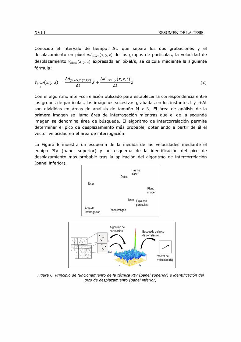
La Figura 6 muestra un esquema de la medida de las velocidades mediante el
equipo PIV (panel superior) y un esquema de la identificación del pico de
desplazamiento más probable tras la aplicación del algoritmo de intercorrelación
(panel inferior).
Figura 6. Principio de funcionamiento de la técnica PIV (panel superior) e identificación del pico de desplazamiento (panel inferior)
Área de interrogación
láser
Plano imagen
Plano imagen
Haz luz láser
Flujo con partículas
lente
Óptica
Búsqueda del pico de correlación
Vector de velocidad (U)
Algoritmo de correlación
RESUMEN DE LA TESIS XIX
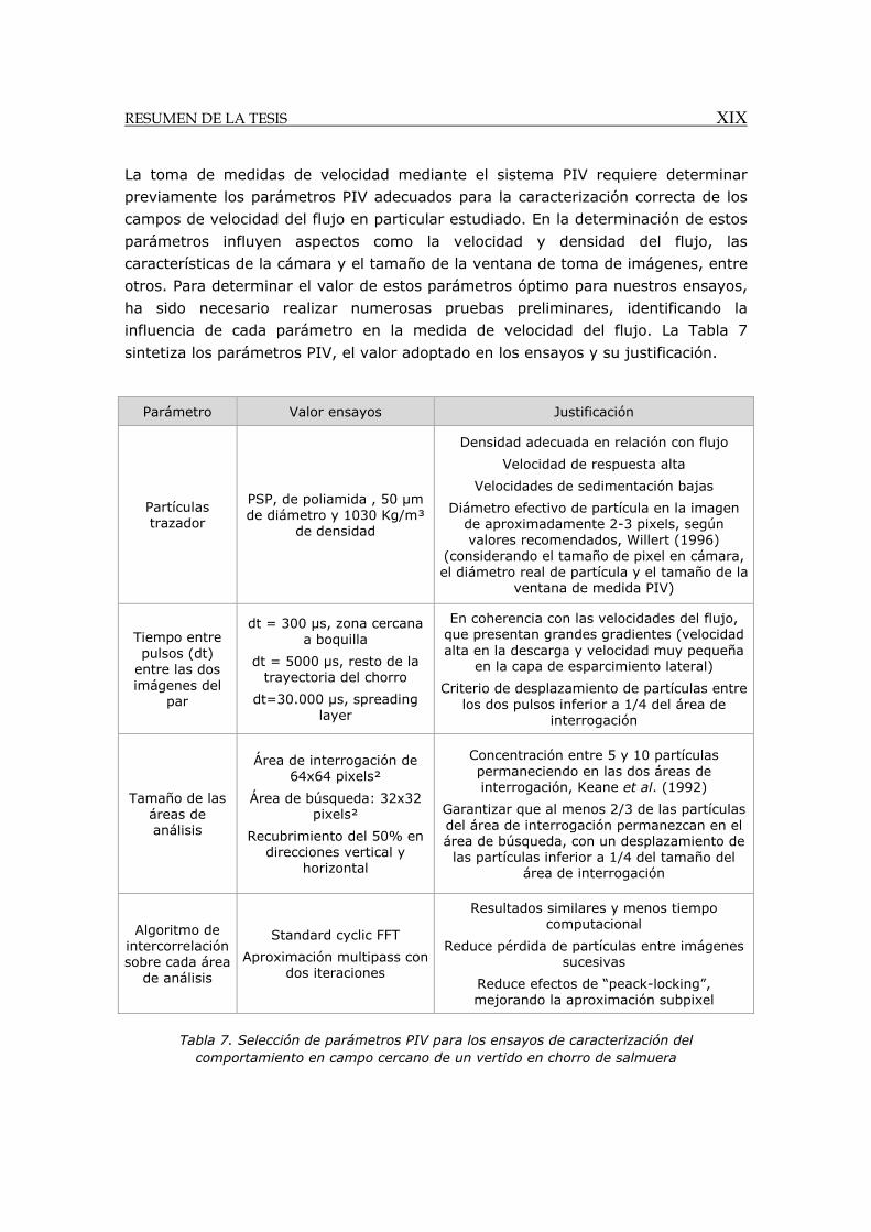
La toma de medidas de velocidad mediante el sistema PIV requiere determinar
previamente los parámetros PIV adecuados para la caracterización correcta de los
campos de velocidad del flujo en particular estudiado. En la determinación de estos
parámetros influyen aspectos como la velocidad y densidad del flujo, las
características de la cámara y el tamaño de la ventana de toma de imágenes, entre
otros. Para determinar el valor de estos parámetros óptimo para nuestros ensayos,
ha sido necesario realizar numerosas pruebas preliminares, identificando la
influencia de cada parámetro en la medida de velocidad del flujo. La Tabla 7
sintetiza los parámetros PIV, el valor adoptado en los ensayos y su justificación.
Tabla 7. Selección de parámetros PIV para los ensayos de caracterización del comportamiento en campo cercano de un vertido en chorro de salmuera
Parámetro Valor ensayos Justificación
Partículas trazador
PSP, de poliamida , 50 µm de diámetro y 1030 Kg/m³
de densidad
Densidad adecuada en relación con flujo
Velocidad de respuesta alta
Velocidades de sedimentación bajas
Diámetro efectivo de partícula en la imagen de aproximadamente 2-3 pixels, según valores recomendados, Willert (1996)
(considerando el tamaño de pixel en cámara, el diámetro real de partícula y el tamaño de la
ventana de medida PIV)
Tiempo entre pulsos (dt)
entre las dos imágenes del
par
dt = 300 µs, zona cercana a boquilla
dt = 5000 μs, resto de la trayectoria del chorro
dt=30.000 µs, spreading layer
En coherencia con las velocidades del flujo, que presentan grandes gradientes (velocidad alta en la descarga y velocidad muy pequeña
en la capa de esparcimiento lateral)
Criterio de desplazamiento de partículas entre los dos pulsos inferior a 1/4 del área de
interrogación
Tamaño de las áreas de análisis
Área de interrogación de 64x64 pixels²
Área de búsqueda: 32x32 pixels²
Recubrimiento del 50% en direcciones vertical y
horizontal
Concentración entre 5 y 10 partículas permaneciendo en las dos áreas de interrogación, Keane et al. (1992)
Garantizar que al menos 2/3 de las partículas del área de interrogación permanezcan en el área de búsqueda, con un desplazamiento de
las partículas inferior a 1/4 del tamaño del área de interrogación
Algoritmo de intercorrelación sobre cada área
de análisis
Standard cyclic FFT
Aproximación multipass con dos iteraciones
Resultados similares y menos tiempo computacional
Reduce pérdida de partículas entre imágenes sucesivas
Reduce efectos de “peack-locking”, mejorando la aproximación subpixel
XX RESUMEN DE LA TESIS
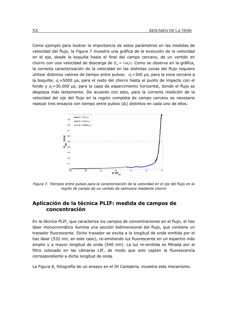
Como ejemplo para ilustrar la importancia de estos parámetros en las medidas de
velocidad del flujo, la Figura 7 muestra una gráfica de la evolución de la velocidad
en el eje, desde la boquilla hasta el final del campo cercano, de un vertido en
chorro con una velocidad de descarga de 1 / . Como se observa en la gráfica,
la correcta caracterización de la velocidad en las distintas zonas del flujo requiere
utilizar distintos valores de tiempo entre pulsos: =300 µs, para la zona cercana a
la boquilla; =5000 µs, para el resto del chorro hasta el punto de impacto con el
fondo y =30.000 µs, para la capa de esparcimiento horizontal, donde el flujo se
desplaza más lentamente. De acuerdo con esto, para la correcta medición de la
velocidad del eje del flujo en la región completa de campo cercano es necesario
realizar tres ensayos con tiempo entre pulsos (dt) distintos en cada uno de ellos.
Figura 7. Tiempos entre pulsos para la caracterización de la velocidad en el eje del flujo en la región de campo de un vertido de salmuera mediante chorro
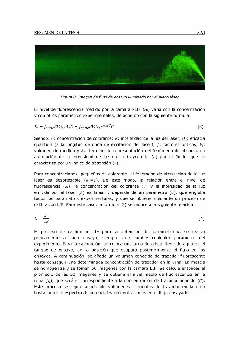
Aplicación de la técnica PLIF: medida de campos de concentración
En la técnica PLIF, que caracteriza los campos de concentraciones en el flujo, el haz
láser monocromático ilumina una sección bidimensional del flujo, que contiene un
trazador fluorescente. Dicho trazador se excita a la longitud de onda emitida por el
haz láser (532 nm, en este caso), re-emitiendo luz fluorescente en un espectro más
amplio y a mayor longitud de onda (540 nm). La luz re-emitida es filtrada por el
filtro colocado en las cámaras LIF, de modo que solo captan la fluorescencia
correspondiente a dicha longitud de onda.
La Figura 8, fotografía de un ensayo en el IH Cantabria, muestra este mecanismo.
RESUMEN DE LA TESIS XXI
Figura 8. Imagen de flujo de ensayo iluminado por el plano láser
El nivel de fluorescencia medido por la cámara PLIF (Sl) varía con la concentración
y con otros parámetros experimentales, de acuerdo con la siguiente fórmula:
3
Siendo: : concentración de colorante; : intensidad de la luz del láser; : eficacia
quantum (a la longitud de onda de excitación del láser); : factores ópticos; :
volumen de medida y : término de representación del fenómeno de absorción o
atenuación de la intensidad de luz en su trayectoria ( ) por el fluido, que se
caracteriza por un índice de absorción ( ).
Para concentraciones pequeñas de colorante, el fenómeno de atenuación de la luz
láser es despreciable ( =1). De este modo, la relación entre el nivel de
fluorescencia ( ), la concentración del colorante ( ) y la intensidad de la luz
emitida por el láser ( ) es linear y depende de un parámetro ( ), que engloba
todos los parámetros experimentales, y que se obtiene mediante un proceso de
calibración LIF. Para este caso, la fórmula (3) se reduce a la siguiente relación:
4
El proceso de calibración LIF para la obtención del parámetro , se realiza
previamente a cada ensayo, siempre que cambie cualquier parámetro del
experimento. Para la calibración, se coloca una urna de cristal llena de agua en el
tanque de ensayo, en la posición que ocupará posteriormente el flujo en los
ensayos. A continuación, se añade un volumen conocido de trazador fluorescente
hasta conseguir una determinada concentración de trazador en la urna. La mezcla
se homogeniza y se toman 50 imágenes con la cámara LIF. Se calcula entonces el
promedio de las 50 imágenes y se obtiene el nivel medio de fluorescencia en la
urna ( ), que será el correspondiente a la concentración de trazador añadido ( ).
Este proceso se repite añadiendo volúmenes crecientes de trazador en la urna
hasta cubrir el espectro de potenciales concentraciones en el flujo ensayado.
XXII RESUMEN DE LA TESIS
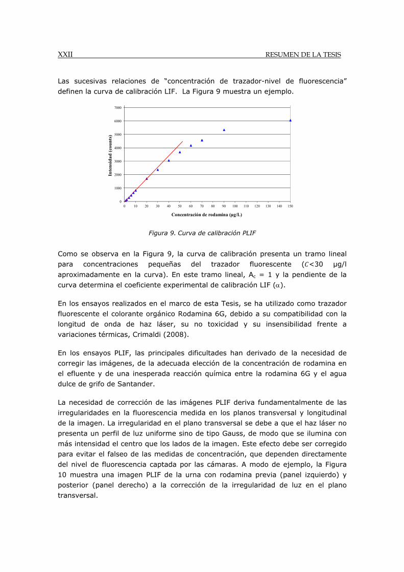
Las sucesivas relaciones de “concentración de trazador-nivel de fluorescencia”
definen la curva de calibración LIF. La Figura 9 muestra un ejemplo.
Figura 9. Curva de calibración PLIF
Como se observa en la Figura 9, la curva de calibración presenta un tramo lineal
para concentraciones pequeñas del trazador fluorescente ( <30 μg/l
aproximadamente en la curva). En este tramo lineal, Ac = 1 y la pendiente de la
curva determina el coeficiente experimental de calibración LIF ().
En los ensayos realizados en el marco de esta Tesis, se ha utilizado como trazador
fluorescente el colorante orgánico Rodamina 6G, debido a su compatibilidad con la
longitud de onda de haz láser, su no toxicidad y su insensibilidad frente a
variaciones térmicas, Crimaldi (2008).
En los ensayos PLIF, las principales dificultades han derivado de la necesidad de
corregir las imágenes, de la adecuada elección de la concentración de rodamina en
el efluente y de una inesperada reacción química entre la rodamina 6G y el agua
dulce de grifo de Santander.
La necesidad de corrección de las imágenes PLIF deriva fundamentalmente de las
irregularidades en la fluorescencia medida en los planos transversal y longitudinal
de la imagen. La irregularidad en el plano transversal se debe a que el haz láser no
presenta un perfil de luz uniforme sino de tipo Gauss, de modo que se ilumina con
más intensidad el centro que los lados de la imagen. Este efecto debe ser corregido
para evitar el falseo de las medidas de concentración, que dependen directamente
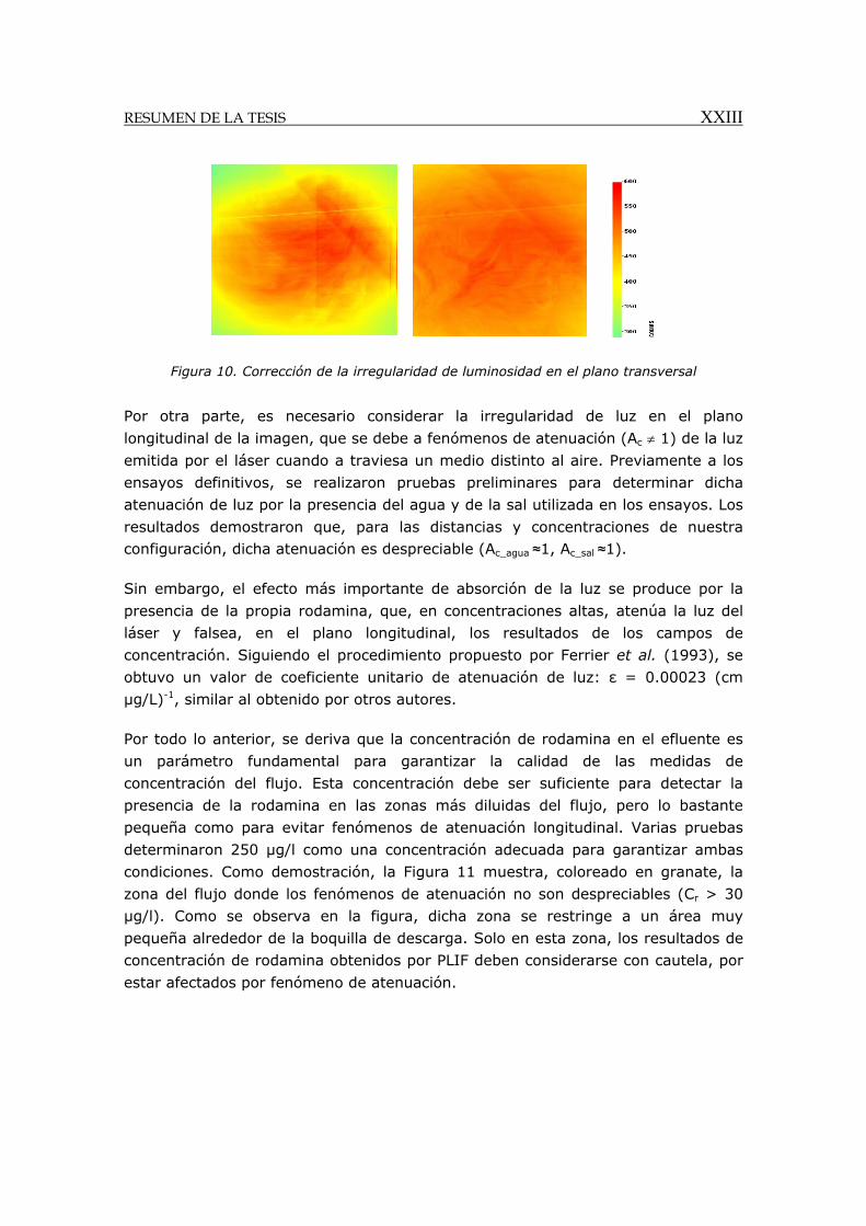
del nivel de fluorescencia captada por las cámaras. A modo de ejemplo, la Figura
10 muestra una imagen PLIF de la urna con rodamina previa (panel izquierdo) y
posterior (panel derecho) a la corrección de la irregularidad de luz en el plano
transversal.
0
1000
2000
3000
4000
5000
6000
7000
0 10 20 30 40 50 60 70 80 90 100 110 120 130 140 150
Inte
nsi
da
d (
cou
nts
)
Concentración de rodamina (µg/L)
RESUMEN DE LA TESIS XXIII
Figura 10. Corrección de la irregularidad de luminosidad en el plano transversal
Por otra parte, es necesario considerar la irregularidad de luz en el plano
longitudinal de la imagen, que se debe a fenómenos de atenuación (Ac 1) de la luz
emitida por el láser cuando a traviesa un medio distinto al aire. Previamente a los
ensayos definitivos, se realizaron pruebas preliminares para determinar dicha
atenuación de luz por la presencia del agua y de la sal utilizada en los ensayos. Los
resultados demostraron que, para las distancias y concentraciones de nuestra configuración, dicha atenuación es despreciable (Ac_agua ≈1, Ac_sal ≈1).
Sin embargo, el efecto más importante de absorción de la luz se produce por la
presencia de la propia rodamina, que, en concentraciones altas, atenúa la luz del
láser y falsea, en el plano longitudinal, los resultados de los campos de
concentración. Siguiendo el procedimiento propuesto por Ferrier et al. (1993), se
obtuvo un valor de coeficiente unitario de atenuación de luz: ε = 0.00023 (cm
µg/L)-1, similar al obtenido por otros autores.
Por todo lo anterior, se deriva que la concentración de rodamina en el efluente es
un parámetro fundamental para garantizar la calidad de las medidas de
concentración del flujo. Esta concentración debe ser suficiente para detectar la
presencia de la rodamina en las zonas más diluidas del flujo, pero lo bastante
pequeña como para evitar fenómenos de atenuación longitudinal. Varias pruebas
determinaron 250 µg/l como una concentración adecuada para garantizar ambas
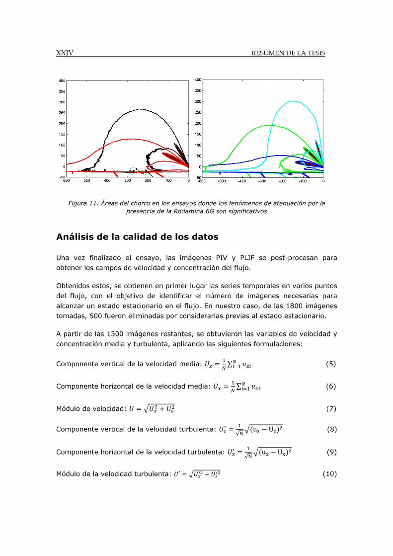
condiciones. Como demostración, la Figura 11 muestra, coloreado en granate, la
zona del flujo donde los fenómenos de atenuación no son despreciables (Cr > 30
µg/l). Como se observa en la figura, dicha zona se restringe a un área muy
pequeña alrededor de la boquilla de descarga. Solo en esta zona, los resultados de
concentración de rodamina obtenidos por PLIF deben considerarse con cautela, por
estar afectados por fenómeno de atenuación.
XXIV RESUMEN DE LA TESIS
Figura 11. Áreas del chorro en los ensayos donde los fenómenos de atenuación por la presencia de la Rodamina 6G son significativos
Análisis de la calidad de los datos
Una vez finalizado el ensayo, las imágenes PIV y PLIF se post-procesan para
obtener los campos de velocidad y concentración del flujo.
Obtenidos estos, se obtienen en primer lugar las series temporales en varios puntos
del flujo, con el objetivo de identificar el número de imágenes necesarias para
alcanzar un estado estacionario en el flujo. En nuestro caso, de las 1800 imágenes
tomadas, 500 fueron eliminadas por considerarlas previas al estado estacionario.
A partir de las 1300 imágenes restantes, se obtuvieron las variables de velocidad y
concentración media y turbulenta, aplicando las siguientes formulaciones:
Componente vertical de la velocidad media: ∑ (5)
Componente horizontal de la velocidad media: ∑ (6)
Módulo de velocidad: (7)
Componente vertical de la velocidad turbulenta: √N
u U (8)
Componente horizontal de la velocidad turbulenta: √N
u U (9)
Módulo de la velocidad turbulenta: (10)
RESUMEN DE LA TESIS XXV
Concentración media: ∑ (11)
Concentración turbulenta (fluctuaciones de concentración): C√N
c C (12)
Vorticidad en el plano x-z: (13)
Dilución neta: (14)
Siendo: , : valores instantaneous de velocidad horizontal y vertical; : valores
instantáneos de concentración; : número de imágenes y : concentración inicial
del efluente.
Considerando estos valores, se ha realizado a continuación un análisis de la
convergencia de los estadísticos, con el fin de determinar si las 1300 imágenes
finales son suficientes para garantizar la convergencia de los estadísticos, de modo
que puedan considerarse representativas del comportamiento real del flujo.
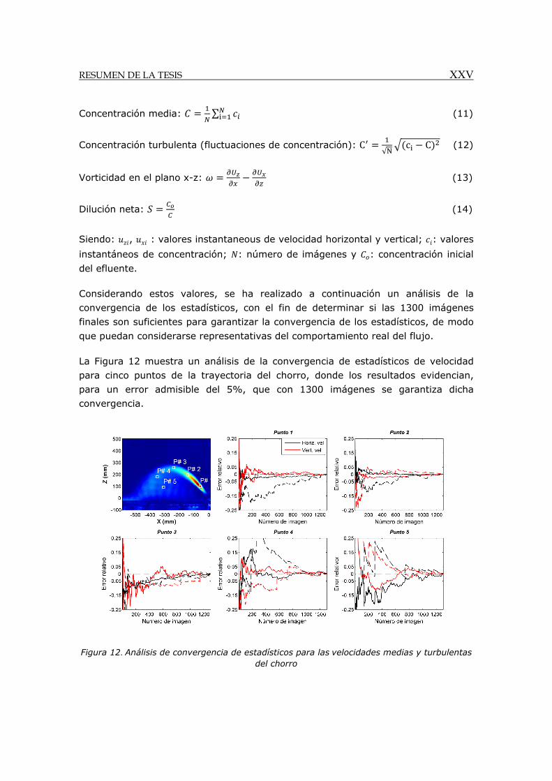
La Figura 12 muestra un análisis de la convergencia de estadísticos de velocidad
para cinco puntos de la trayectoria del chorro, donde los resultados evidencian,
para un error admisible del 5%, que con 1300 imágenes se garantiza dicha
convergencia.
Figura 12. Análisis de convergencia de estadísticos para las velocidades medias y turbulentas del chorro
XXVI RESUMEN DE LA TESIS
CARACTERIZACIÓN DEL COMPORTAMIENTO DEL CHORRO EN BASE AL ANÁLISIS DE DATOS EXPERIMENTALES
Para la caracterización del chorro se realizaron un total de 15 ensayos, escalando a
1:40 un prototipo de vertido de salmuera en el Mar Mediterráneo, mediante un
emisario submarino con chorro sumergido e inclinado. Como parámetros variables,
se consideran el ángulo de descarga ( ) y el Número de Froude Densimétrico ( )
Para asumir flujo turbulento completamente desarrollado y poder garantizar la
semejanza dinámica mediante la igualdad en el Número de Froude Densimétrico, se
ha deducido mediante ensayos previos la necesidad de Números de Reynolds en el
flujo superiores a 2000. Por otra parte, para aplicar análisis dimensional
despreciando el flujo de caudal en la fuente, se ha obtenido que el Número de
Froude Densimétrico del chorro ha de ser mayor que 15 en nuestros ensayos. Para
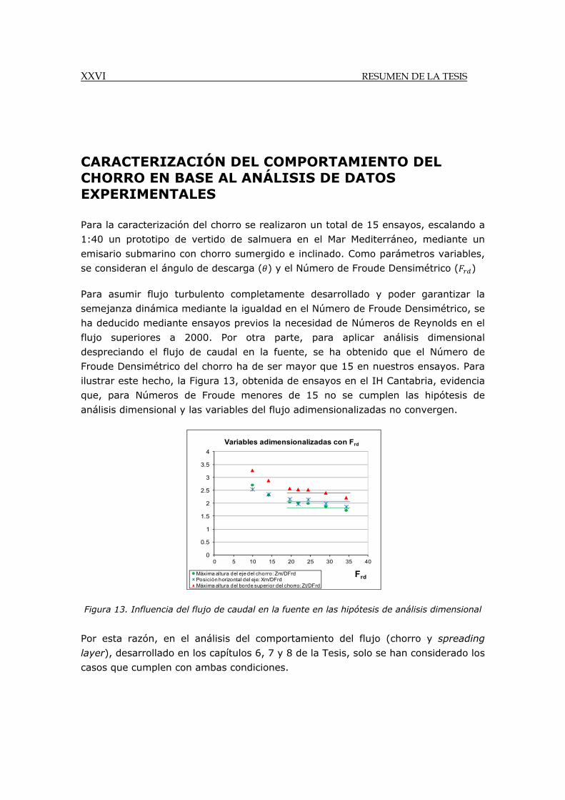
ilustrar este hecho, la Figura 13, obtenida de ensayos en el IH Cantabria, evidencia
que, para Números de Froude menores de 15 no se cumplen las hipótesis de
análisis dimensional y las variables del flujo adimensionalizadas no convergen.
Figura 13. Influencia del flujo de caudal en la fuente en las hipótesis de análisis dimensional
Por esta razón, en el análisis del comportamiento del flujo (chorro y spreading
layer), desarrollado en los capítulos 6, 7 y 8 de la Tesis, solo se han considerado los
casos que cumplen con ambas condiciones.
0
0.5
1
1.5
2
2.5
3
3.5
4
0 5 10 15 20 25 30 35 40
Frd
Variables adimensionalizadas con Frd
Máxima altura del eje del chorro: Zm/DFrdPosición horizontal del eje: Xm/DFrdMáxima altura del borde superior del chorro: Zt/DFrd
RESUMEN DE LA TESIS XXVII
Evolución de las variables en los ejes. Análisis dimensional
Como primer paso del análisis se han obtenido mediante un proceso iterativo los
ejes de velocidad y concentración del chorro, que corresponden a las líneas que
unen los puntos de máxima velocidad y concentración en las secciones
transversales del flujo.
Los resultados muestran la convergencia entre ambos ejes a lo largo de la
trayectoria ascendente del chorro, mientras que a partir de cierta posición de su
trayectoria descendente, divergen. El eje de concentraciones presenta siempre una
mayor pendiente en la trayectoria de descenso y tras impactar con el fondo, se
impone la condición de contorno de no-flujo, que provoca la acumulación del flujo y
la posición del eje del concentración justo pegado al fondo.
Definidos los ejes, se ha obtenido la evolución de las variables a lo largo de los
mismos para chorros con distintas inclinaciones. Para comparar los distintos casos,
se han aplicado fórmulas de análisis dimensional, normalizando las variables
mediante el diámetro de la boquilla ( ), el Número de Froude Densimétrico
( ) y la velocidad en la descarga ( ).
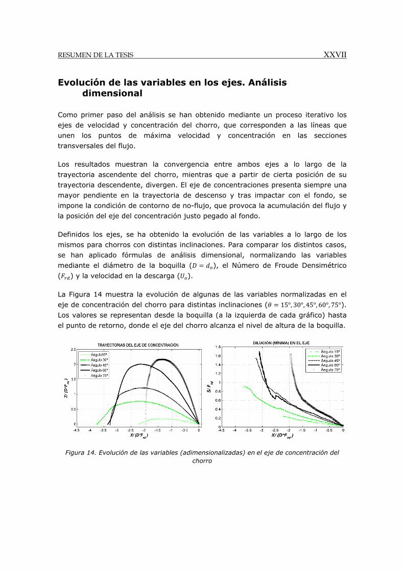
La Figura 14 muestra la evolución de algunas de las variables normalizadas en el
eje de concentración del chorro para distintas inclinaciones ( 15°, 30°, 45°, 60°, 75°).
Los valores se representan desde la boquilla (a la izquierda de cada gráfico) hasta
el punto de retorno, donde el eje del chorro alcanza el nivel de altura de la boquilla.
Figura 14. Evolución de las variables (adimensionalizadas) en el eje de concentración del chorro
XXVIII RESUMEN DE LA TESIS
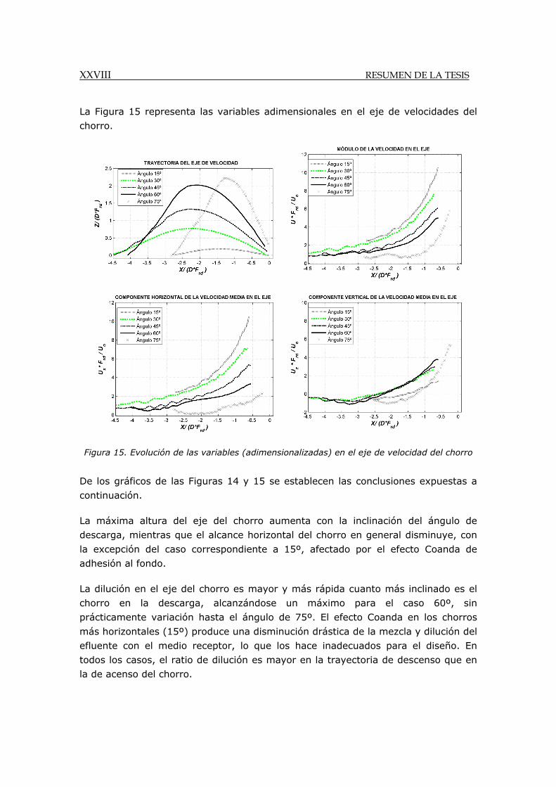
La Figura 15 representa las variables adimensionales en el eje de velocidades del
chorro.
Figura 15. Evolución de las variables (adimensionalizadas) en el eje de velocidad del chorro
De los gráficos de las Figuras 14 y 15 se establecen las conclusiones expuestas a
continuación.
La máxima altura del eje del chorro aumenta con la inclinación del ángulo de
descarga, mientras que el alcance horizontal del chorro en general disminuye, con
la excepción del caso correspondiente a 15º, afectado por el efecto Coanda de
adhesión al fondo.
La dilución en el eje del chorro es mayor y más rápida cuanto más inclinado es el
chorro en la descarga, alcanzándose un máximo para el caso 60º, sin
prácticamente variación hasta el ángulo de 75º. El efecto Coanda en los chorros
más horizontales (15º) produce una disminución drástica de la mezcla y dilución del
efluente con el medio receptor, lo que los hace inadecuados para el diseño. En
todos los casos, el ratio de dilución es mayor en la trayectoria de descenso que en
la de acenso del chorro.
RESUMEN DE LA TESIS XXIX
Se observa (aunque no se presentan los gráficos en este resumen) que la dilución
en el punto de retorno es mayor en el punto de retorno que en punto de impacto
del chorro con el fondo, debido a que en esta zona se forma una acumulación del
flujo por la presencia del fondo.
En relación con las variables hidrodinámicas, la componente horizontal de
momentum decrece continuamente desde la boquilla hasta el punto de retorno,
debido al rozamiento del flujo con el fluido receptor en reposo. La componente
vertical de momentum decrece rápidamente desde la boquilla por efecto combinado
del rozamiento y de la gravedad. Cuando el momentum y la flotabilidad se igualan,
la velocidad vertical se anula y el chorro alcanza su máxima altura. A partir de ese
punto, comienza su trayectoria de descenso, aumentando, aunque con signo
contrario, el valor de la velocidad por efecto de la gravedad.
Considerando las variables en global, se puede concluir que la dilución parece
depender fundamentalmente de la longitud de la trayectoria del chorro ( ) y de la
componente vertical de la velocidad ( ), siendo la dilución mayor cuanto mayor es
el valor de estas dos variables.
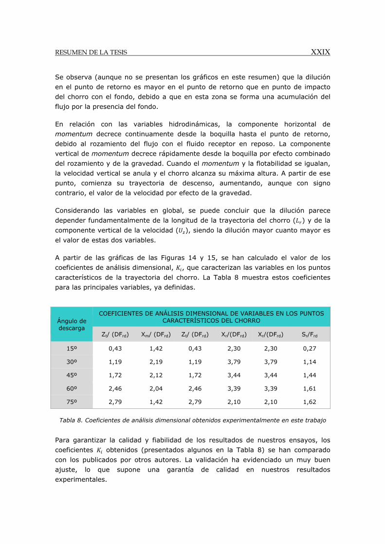
A partir de las gráficas de las Figuras 14 y 15, se han calculado el valor de los
coeficientes de análisis dimensional, , que caracterizan las variables en los puntos
característicos de la trayectoria del chorro. La Tabla 8 muestra estos coeficientes
para las principales variables, ya definidas.
Tabla 8. Coeficientes de análisis dimensional obtenidos experimentalmente en este trabajo
Para garantizar la calidad y fiabilidad de los resultados de nuestros ensayos, los
coeficientes obtenidos (presentados algunos en la Tabla 8) se han comparado
con los publicados por otros autores. La validación ha evidenciado un muy buen
ajuste, lo que supone una garantía de calidad en nuestros resultados
experimentales.
Ángulo de descarga
COEFICIENTES DE ANÁLISIS DIMENSIONAL DE VARIABLES EN LOS PUNTOS CARACTERÍSTICOS DEL CHORRO
Zt/ (DFrd) Xm/ (DFrd) Zt/ (DFrd) Xr/(DFrd) Xr/(DFrd) Sr/Frd
15º 0,43 1,42 0,43 2,30 2,30 0,27
30º 1,19 2,19 1,19 3,79 3,79 1,14
45º 1,72 2,12 1,72 3,44 3,44 1,44
60º 2,46 2,04 2,46 3,39 3,39 1,61
75º 2,79 1,42 2,79 2,10 2,10 1,62
XXX RESUMEN DE LA TESIS
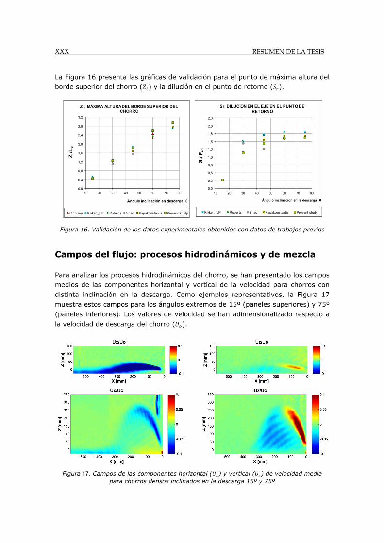
La Figura 16 presenta las gráficas de validación para el punto de máxima altura del
borde superior del chorro ( ) y la dilución en el punto de retorno ( ).
Figura 16. Validación de los datos experimentales obtenidos con datos de trabajos previos
Campos del flujo: procesos hidrodinámicos y de mezcla
Para analizar los procesos hidrodinámicos del chorro, se han presentado los campos
medios de las componentes horizontal y vertical de la velocidad para chorros con
distinta inclinación en la descarga. Como ejemplos representativos, la Figura 17
muestra estos campos para los ángulos extremos de 15º (paneles superiores) y 75º
(paneles inferiores). Los valores de velocidad se han adimensionalizado respecto a
la velocidad de descarga del chorro ( ).
Figura 17. Campos de las componentes horizontal ( ) y vertical ( ) de velocidad media para chorros densos inclinados en la descarga 15º y 75º
0,0
0,4
0,8
1,2
1,6
2,0
2,4
2,8
3,2
10 20 30 40 50 60 70 80
Zt /
LM
Angulo inclinación en descarga, θ
Zt: MÁXIMA ALTURA DEL BORDE SUPERIOR DEL CHORRO
Cipollina Kikkert_LIF Roberts Shao Papakonstantis Present study
0,0
0,3
0,5
0,8
1,0
1,3
1,5
1,8
2,0
2,3
10 20 30 40 50 60 70 80
Sr/ F
rdÁngulo inclinación en la descarga, θ
Sr: DILUCION EN EL EJE EN EL PUNTO DE RETORNO
Kikkert_LIF Roberts Shao Papakonstantis Present study
RESUMEN DE LA TESIS XXXI
Como se observa en la Figura 17, la componente horizontal de momentum
disminuye a lo largo de la trayectoria del chorro, debido al rozamiento con el fluido
receptor en reposo. Cuando el chorro impacto el fondo, el momentum total se
transforma en momentum horizontal, formándose una capa densa (spreading layer)
que se expande sobre el fondo. Los campos de componente horizontal de velocidad
muestran además la presencia de estructuras coherentes ocupando la sección
transversal del flujo, cuya forma pasa de ser elíptica, en las secciones cercanas a la
boquilla, a prácticamente circular, cerca del punto de impacto.
La componente vertical de momentum disminuye rápidamente desde la boquilla
hasta el punto de máxima altura, debido al efecto combinado de la gravedad y del
rozamiento. En dicho punto, la velocidad vertical es nula y a partir de entonces
cambia de dirección (valores negativos), aumentando su valor por valor por efecto
de la gravedad, pero en menor grado, dado que flotabilidad y fricción tienen efectos
contrarios sobre el chorro.
En todos los casos, especialmente en chorros con inclinaciones altas en la descarga,
se observa en los campos de momentum vertical, un flujo de caída disperso en la
rama descendente de la trayectoria, aproximándose más a un comportamiento tipo
pluma que tipo chorro. Se observa además en estas zonas, la existencia de
estructuras coherentes que muestran caminos preferenciales en la caída del flujo.
Para profundizar en los procesos hidrodinámicos de estos chorros de flotabilidad
negativa y comparar su comportamiento respecto al de chorros neutros, se han
obtenido los campos de vorticidad plana del flujo, que permiten caracterizar los
movimientos rotacionales del flujo.
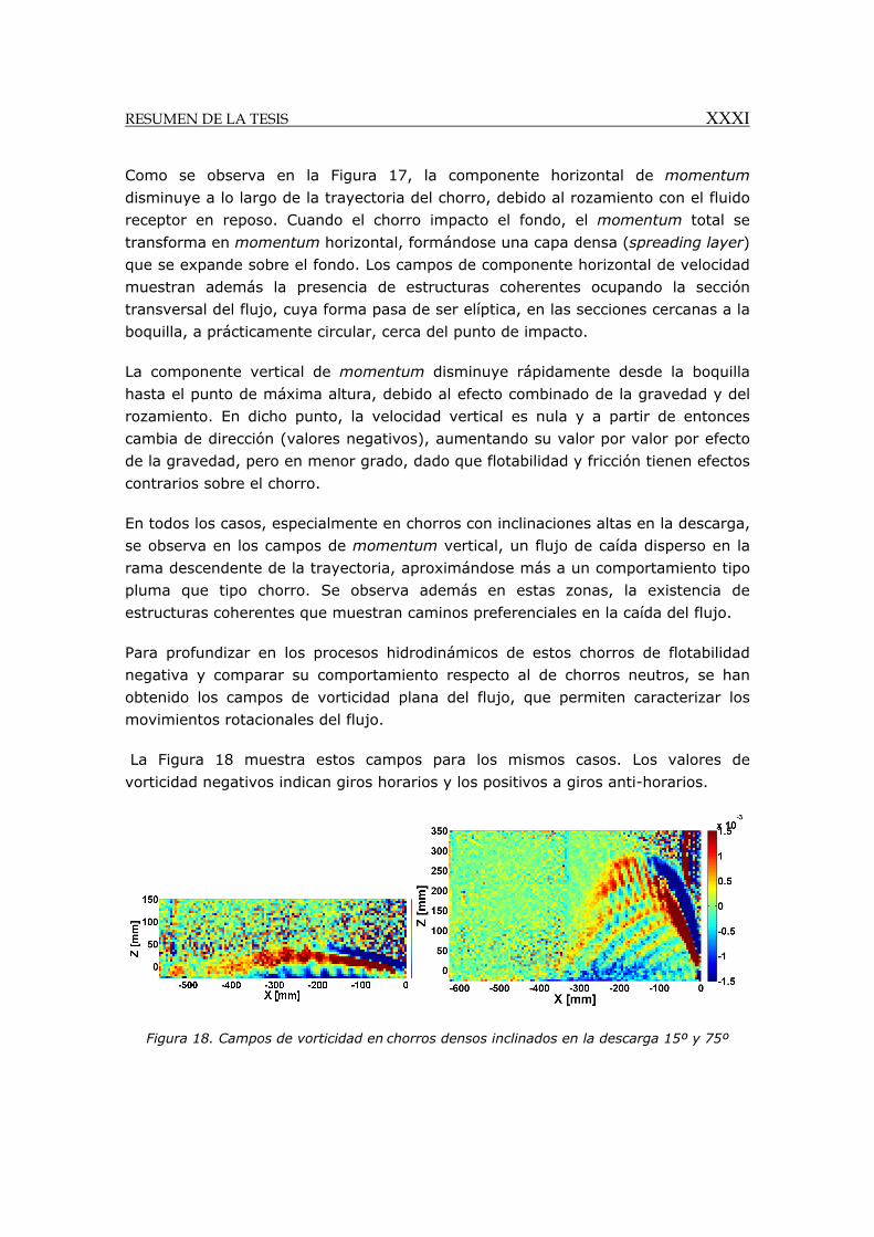
La Figura 18 muestra estos campos para los mismos casos. Los valores de
vorticidad negativos indican giros horarios y los positivos a giros anti-horarios.
Figura 18. Campos de vorticidad en chorros densos inclinados en la descarga 15º y 75º
XXXII RESUMEN DE LA TESIS
En un chorro neutro, los campos de vorticidad revelan un flujo girando en sentido
horario en la mitad superior del chorro y en sentido anti-horario en la mitad
inferior, separados ambos flujos por eje del chorro, donde la vorticidad es nula.
Observando los campos de vorticidad para chorros inclinados y de flotabilidad
negativa, este patrón de comportamiento se observa solamente en la rama
ascendente del chorro. En la rama descendente, este comportamiento desaparece,
observándose un flujo más disperso. En particular, se aprecia la existencia de
pequeños vórtices que, girando en sentido anti-horario, se desprenden desde el
borde inferior del flujo y caen casi hacia el fondo por efecto de la gravedad. Estos
vórtices son inestabilidades asociadas a la flotabilidad y se traducen en una cascada
de flujo disperso, que aleja a este tipo de chorros inclinados y con flotabilidad
negativa del comportamiento clásico de chorros neutros.
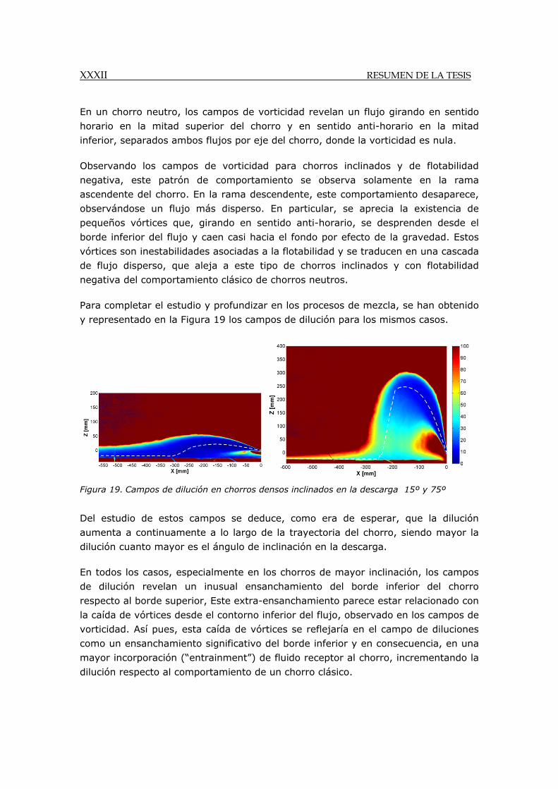
Para completar el estudio y profundizar en los procesos de mezcla, se han obtenido
y representado en la Figura 19 los campos de dilución para los mismos casos.
Figura 19. Campos de dilución en chorros densos inclinados en la descarga 15º y 75º
Del estudio de estos campos se deduce, como era de esperar, que la dilución
aumenta a continuamente a lo largo de la trayectoria del chorro, siendo mayor la
dilución cuanto mayor es el ángulo de inclinación en la descarga.
En todos los casos, especialmente en los chorros de mayor inclinación, los campos
de dilución revelan un inusual ensanchamiento del borde inferior del chorro
respecto al borde superior, Este extra-ensanchamiento parece estar relacionado con
la caída de vórtices desde el contorno inferior del flujo, observado en los campos de
vorticidad. Así pues, esta caída de vórtices se reflejaría en el campo de diluciones
como un ensanchamiento significativo del borde inferior y en consecuencia, en una
mayor incorporación (“entrainment”) de fluido receptor al chorro, incrementando la
dilución respecto al comportamiento de un chorro clásico.
RESUMEN DE LA TESIS XXXIII
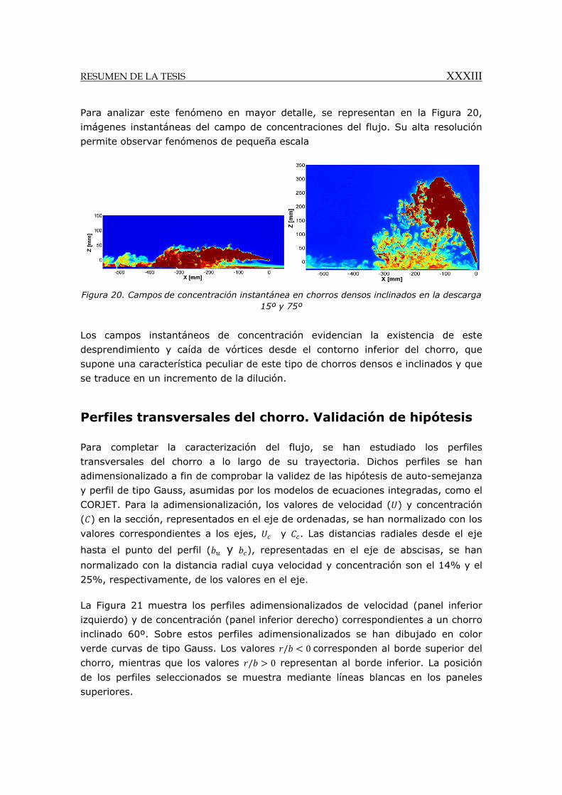
Para analizar este fenómeno en mayor detalle, se representan en la Figura 20,
imágenes instantáneas del campo de concentraciones del flujo. Su alta resolución
permite observar fenómenos de pequeña escala
Figura 20. Campos de concentración instantánea en chorros densos inclinados en la descarga 15º y 75º
Los campos instantáneos de concentración evidencian la existencia de este
desprendimiento y caída de vórtices desde el contorno inferior del chorro, que
supone una característica peculiar de este tipo de chorros densos e inclinados y que
se traduce en un incremento de la dilución.
Perfiles transversales del chorro. Validación de hipótesis
Para completar la caracterización del flujo, se han estudiado los perfiles
transversales del chorro a lo largo de su trayectoria. Dichos perfiles se han
adimensionalizado a fin de comprobar la validez de las hipótesis de auto-semejanza
y perfil de tipo Gauss, asumidas por los modelos de ecuaciones integradas, como el
CORJET. Para la adimensionalización, los valores de velocidad ( ) y concentración
( ) en la sección, representados en el eje de ordenadas, se han normalizado con los
valores correspondientes a los ejes, y . Las distancias radiales desde el eje
hasta el punto del perfil ( y ), representadas en el eje de abscisas, se han
normalizado con la distancia radial cuya velocidad y concentración son el 14% y el
25%, respectivamente, de los valores en el eje.
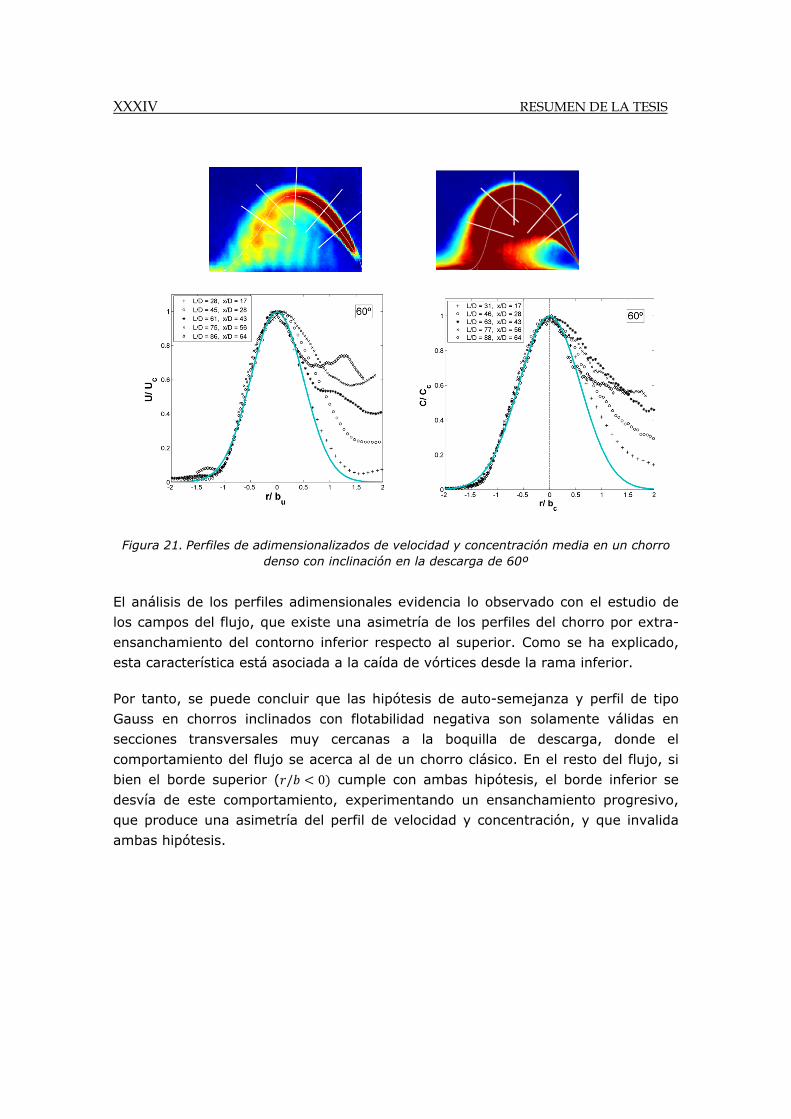
La Figura 21 muestra los perfiles adimensionalizados de velocidad (panel inferior
izquierdo) y de concentración (panel inferior derecho) correspondientes a un chorro
inclinado 60º. Sobre estos perfiles adimensionalizados se han dibujado en color
verde curvas de tipo Gauss. Los valores / 0 corresponden al borde superior del
chorro, mientras que los valores / 0 representan al borde inferior. La posición
de los perfiles seleccionados se muestra mediante líneas blancas en los paneles
superiores.
XXXIV RESUMEN DE LA TESIS
Figura 21. Perfiles de adimensionalizados de velocidad y concentración media en un chorro denso con inclinación en la descarga de 60º
El análisis de los perfiles adimensionales evidencia lo observado con el estudio de
los campos del flujo, que existe una asimetría de los perfiles del chorro por extra-
ensanchamiento del contorno inferior respecto al superior. Como se ha explicado,
esta característica está asociada a la caída de vórtices desde la rama inferior.
Por tanto, se puede concluir que las hipótesis de auto-semejanza y perfil de tipo
Gauss en chorros inclinados con flotabilidad negativa son solamente válidas en
secciones transversales muy cercanas a la boquilla de descarga, donde el
comportamiento del flujo se acerca al de un chorro clásico. En el resto del flujo, si
bien el borde superior ( / 0 cumple con ambas hipótesis, el borde inferior se
desvía de este comportamiento, experimentando un ensanchamiento progresivo,
que produce una asimetría del perfil de velocidad y concentración, y que invalida
ambas hipótesis.
RESUMEN DE LA TESIS XXXV
CARACTERIZACIÓN DE LA CAPA DE ESPARCIMIENTO LATERAL EN BASE AL ANÁLISIS DE LOS DATOS EXPERIMENTALES
Para completar el estudio del comportamiento en campo cercano de un vertido de
salmuera mediante chorro sumergido, se ha realizado un segundo grupo de
ensayos a fin de caracterizar la capa de esparcimiento lateral (spreading layer) que
se forma tras el impacto del chorro con el fondo. Esta capa densa define el tramo
final del campo cercano y la transición al campo lejano, donde el flujo forma una
pluma hipersalina que se desplaza lentamente sobre el fondo.
Existen en la literatura escasos estudios experimentales de caracterización de esta
capa de esparcimiento en el caso de chorros de flotabilidad negativa. De los
existentes, la mayor parte describe la evolución de su expansión horizontal sobre el
fondo, Papakonstantis et al. (2010), entre otros. En relación con la aplicación de
técnicas ópticas al estudio de esta capa, solamente se ha encontrado la publicación
de Roberts et al. (1997), que calibra fórmulas de análisis dimensional para sus
principales características, pero sin profundizar en su comportamiento.
Siguiendo el mismo esquema que en el estudio del chorro, se han analizado los
campos medios y turbulentos del flujo, se han adimensionalizado las variables a lo
largo de los ejes y se han obtenido los perfiles transversales de la spreading layer,
sintetizando a continuación los resultados.
Campos de flujo. Procesos hidrodinámicos y de mezcla
Para comprender los procesos hidrodinámicos y de mezcla, se han obtenido los
campos más representativos de estos procesos en capas de esparcimiento
derivadas de chorros de flotabilidad negativa con distinto ángulo de descarga.
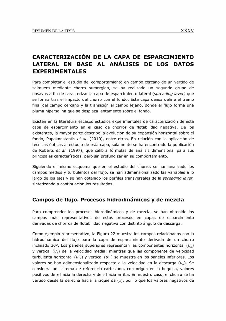
Como ejemplo representativo, la Figura 22 muestra los campos relacionados con la
hidrodinámica del flujo para la capa de esparcimiento derivada de un chorro
inclinado 30º. Los paneles superiores representan las componentes horizontal ( )
y vertical ( ) de la velocidad media; mientras que las componente de velocidad
turbulenta horizontal ( ) y vertical ( ) se muestra en los paneles inferiores. Los
valores se han adimensionalizado respecto a la velocidad en la descarga ( ). Se
considera un sistema de referencia cartesiano, con origen en la boquilla, valores
positivos de hacia la derecha y de hacia arriba. En nuestro caso, el chorro se ha
vertido desde la derecha hacia la izquierda ( , por lo que los valores negativos de
XXXVI RESUMEN DE LA TESIS
abscisas coinciden con la dirección de la descarga. La posición del eje de
velocidades se representa mediante una línea blanca discontinua.
Figura 22. Campos hidrodinámicos de la capa de esparcimiento lateral derivada de un chorro densos con inclinación en la descarga de 30º
De los campos de velocidades medias ( , ), se deduce que el momentum en la
capa de esparcimiento es totalmente horizontal, siendo la componente vertical de la
velocidad despreciable en todos los casos estudiados.
Como se observa en la Figura 22, la velocidad horizontal media disminuye
progresivamente, lo que es debido al rozamiento con el fondo y a la incorporación
(“entrainment”) de fluido receptor a la capa densa. Comparando los campos de
velocidad en capas derivadas de chorros con distinto ángulo de descarga, se
observan mayor velocidad horizontal a menor ángulo.
Las componentes de velocidad turbulenta ( , ) en la spreading presentan
valores similares entre sí. En todos los casos, su valor es elevado tras el punto de
impacto del chorro con el fondo y se va reduciendo a lo largo de la capa de
esparcimiento. Este hecho revela la continua disipación de los procesos turbulentos
en el flujo a lo largo de esta capa. A cierta distancia del punto de vertido, las
fluctuaciones de velocidad son despreciables, revelando el final del campo cercano
y el comienzo del campo lejano.
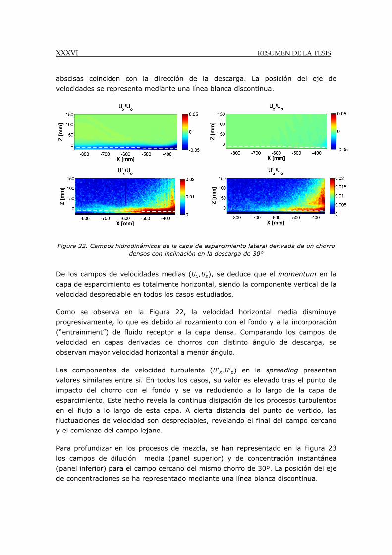
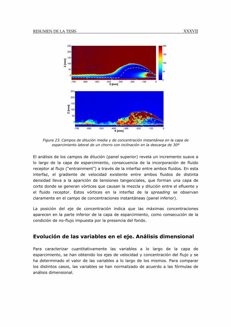
Para profundizar en los procesos de mezcla, se han representado en la Figura 23
los campos de dilución media (panel superior) y de concentración instantánea
(panel inferior) para el campo cercano del mismo chorro de 30º. La posición del eje
de concentraciones se ha representado mediante una línea blanca discontinua.
RESUMEN DE LA TESIS XXXVII
Figura 23. Campos de dilución media y de concentración instantánea en la capa de esparcimiento lateral de un chorro con inclinación en la descarga de 30º
El análisis de los campos de dilución (panel superior) revela un incremento suave a
lo largo de la capa de esparcimiento, consecuencia de la incorporación de fluido
receptor al flujo (“entrainment”) a través de la interfaz entre ambos fluidos. En esta
interfaz, el gradiente de velocidad existente entre ambos fluidos de distinta
densidad lleva a la aparición de tensiones tangenciales, que forman una capa de
corte donde se generan vórtices que causan la mezcla y dilución entre el efluente y
el fluido receptor. Estos vórtices en la interfaz de la spreading se observan
claramente en el campo de concentraciones instantáneas (panel inferior).
La posición del eje de concentración indica que las máximas concentraciones
aparecen en la parte inferior de la capa de esparcimiento, como consecución de la
condición de no-flujo impuesta por la presencia del fondo.
Evolución de las variables en el eje. Análisis dimensional
Para caracterizar cuantitativamente las variables a lo largo de la capa de
esparcimiento, se han obtenido los ejes de velocidad y concentración del flujo y se
ha determinado el valor de las variables a lo largo de los mismos. Para comparar
los distintos casos, las variables se han normalizado de acuerdo a las fórmulas de
análisis dimensional.
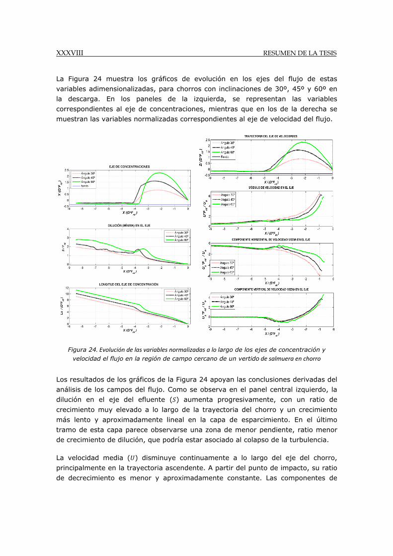
XXXVIII RESUMEN DE LA TESIS
La Figura 24 muestra los gráficos de evolución en los ejes del flujo de estas
variables adimensionalizadas, para chorros con inclinaciones de 30º, 45º y 60º en
la descarga. En los paneles de la izquierda, se representan las variables
correspondientes al eje de concentraciones, mientras que en los de la derecha se
muestran las variables normalizadas correspondientes al eje de velocidad del flujo.
Figura 24. Evolución de las variables normalizadas a lo largo de los ejes de concentración y velocidad el flujo en la región de campo cercano de un vertido de salmuera en chorro
Los resultados de los gráficos de la Figura 24 apoyan las conclusiones derivadas del
análisis de los campos del flujo. Como se observa en el panel central izquierdo, la
dilución en el eje del efluente ( ) aumenta progresivamente, con un ratio de
crecimiento muy elevado a lo largo de la trayectoria del chorro y un crecimiento
más lento y aproximadamente lineal en la capa de esparcimiento. En el último
tramo de esta capa parece observarse una zona de menor pendiente, ratio menor
de crecimiento de dilución, que podría estar asociado al colapso de la turbulencia.
La velocidad media ( ) disminuye continuamente a lo largo del eje del chorro,
principalmente en la trayectoria ascendente. A partir del punto de impacto, su ratio
de decrecimiento es menor y aproximadamente constante. Las componentes de
RESUMEN DE LA TESIS XXXIX
velocidad revelan un movimiento claramente horizontal en la spreading layer,
siendo nula la componente vertical.
Como punto característico del comportamiento de la capa de esparcimiento, se ha
considerado el final del campo cercano. Para esta localización, se han obtenido los
coeficientes de análisis dimensional de las principales variables de la spreading
layer (alcance, espesor, dilución, etc.) para los ángulos de descarga estudiados. Al
comparar estos coeficientes con los disponibles en la literatura, Roberts et al.
(1997), se ha obtenido un muy buen ajuste, lo que implica una garantía de la
coherencia y calidad de nuestros datos experimentales en la spreading layer.
Perfiles transversales
Para finalizar con la caracterización de la capa de esparcimiento lateral, se han
obtenido y analizado los perfiles transversales de velocidad y concentración en
cinco posiciones equidistantes.
Los perfiles se han adimensionalizado para analizar la auto-semejanza entre
secciones y la forma del perfil. Los valores de velocidad y concentración ( , , , ),
representados en el eje de abscisas, se han normalizado mediante los valores
correspondientes al eje del flujo ( , , , ). En el eje de ordenadas, siguiendo lo
propuesto por Mingyu Liu et al. (2003), la distancia vertical respecto al fondo ( se
ha adimensionalizado con el valor de la distancia desde el fondo hasta el punto
donde la velocidad y concentración son la mitad de los valores en los ejes ( / ,
/ , / , / ).
La Figura 25 muestra estos perfiles para la spreading layer de un chorro con
inclinación en la descarga de 60º.
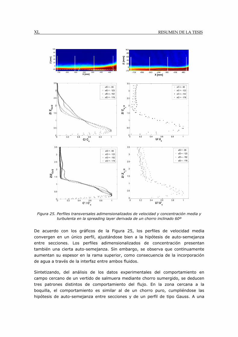
XL RESUMEN DE LA TESIS
Figura 25. Perfiles transversales adimensionalizados de velocidad y concentración media y turbulenta en la spreading layer derivada de un chorro inclinado 60º
De acuerdo con los gráficos de la Figura 25, los perfiles de velocidad media
convergen en un único perfil, ajustándose bien a la hipótesis de auto-semejanza
entre secciones. Los perfiles adimensionalizados de concentración presentan
también una cierta auto-semejanza. Sin embargo, se observa que continuamente
aumentan su espesor en la rama superior, como consecuencia de la incorporación
de agua a través de la interfaz entre ambos fluidos.
Sintetizando, del análisis de los datos experimentales del comportamiento en
campo cercano de un vertido de salmuera mediante chorro sumergido, se deducen
tres patrones distintos de comportamiento del flujo. En la zona cercana a la
boquilla, el comportamiento es similar al de un chorro puro, cumpliéndose las
hipótesis de auto-semejanza entre secciones y de un perfil de tipo Gauss. A una
RESUMEN DE LA TESIS XLI
distancia pequeña desde la boquilla, aparecen inestabilidades en el flujo por efecto
de la flotabilidad negativa, desprendiéndose desde la rama inferior vórtices que
caen en forma de cascada. Este hecho genera asimetría en los perfiles,
incrementando la dilución e invalidando las mencionadas hipótesis. Finalmente, tras
el impacto del chorro con el fondo, el flujo se transforma en una capa densa
horizontal que se expande en todas direcciones, reduciéndose continuamente el
valor de las fluctuaciones hasta su colapso, zona donde se considera el final del
comportamiento en campo cercano y el comienzo del campo lejano.
NUEVOS MODELOS “BRIHNE” PARA LA SIMULACIÓN DE VERTIDOS DE SALMUERA
Las limitaciones de los modelos de simulación comerciales y su deficiente ajuste a
los datos experimentales generan incertidumbres significativas en la predicción del
comportamiento del vertido de salmuera, y, por tanto, en la garantía de protección
del medio marino. Estas razones, junto con la imposibilidad de acceder a sus
códigos para mejorarlos y re-calibrarlos, ha llevado a plantear el diseño de nuevas
herramientas de modelado.
Este objetivo se ha materializado en el desarrollo de las herramientas “brIHne”,
enfocadas en la simulación de vertidos al mar de salmuera, y que predicen su
comportamiento bajo diferentes configuraciones de descarga y con distintos
ámbitos de aplicación, incluyendo campo cercano y campo lejano.
Los modelos “BriHne” se basan en las aproximaciones numéricas de análisis
dimensional y de ecuaciones integradas, habiendo seleccionado las formulaciones
más adecuadas entre las disponibles en publicaciones científicas. Programadas en
Matlab, una ventaja importante de las herramientas “brIHne” frente a las
comerciales es su re-calibración con los datos experimentales obtenidos mediante
técnicas ópticas PIV-PLIF en el IH Cantabria. Además, la disponibilidad de los
códigos permite su mejora continua, incorporando nuevas opciones a medida que
se disponga de datos experimentales para la calibración. En la misma línea que el
resto de los trabajos de la Tesis, los modelos “brIHne” desarrollados hasta el
momento se centran en salmuera procedente de plantas desaladoras de ósmosis
inversa y en descargas mediante chorros sumergidos en un medio receptor en
reposo y dinámico.
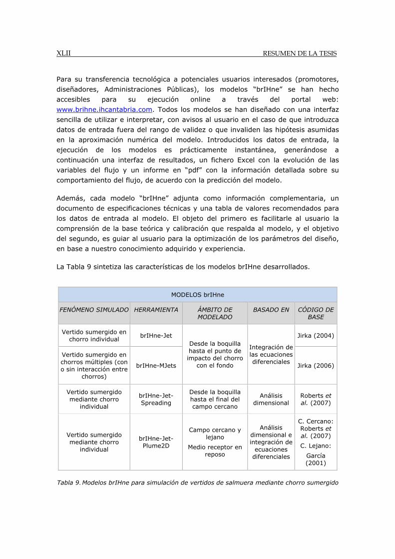
XLII RESUMEN DE LA TESIS
Para su transferencia tecnológica a potenciales usuarios interesados (promotores,
diseñadores, Administraciones Públicas), los modelos “brIHne” se han hecho
accesibles para su ejecución online a través del portal web:
www.brihne.ihcantabria.com. Todos los modelos se han diseñado con una interfaz
sencilla de utilizar e interpretar, con avisos al usuario en el caso de que introduzca
datos de entrada fuera del rango de validez o que invaliden las hipótesis asumidas
en la aproximación numérica del modelo. Introducidos los datos de entrada, la
ejecución de los modelos es prácticamente instantánea, generándose a
continuación una interfaz de resultados, un fichero Excel con la evolución de las
variables del flujo y un informe en “pdf” con la información detallada sobre su
comportamiento del flujo, de acuerdo con la predicción del modelo.
Además, cada modelo “brIHne” adjunta como información complementaria, un
documento de especificaciones técnicas y una tabla de valores recomendados para
los datos de entrada al modelo. El objeto del primero es facilitarle al usuario la
comprensión de la base teórica y calibración que respalda al modelo, y el objetivo
del segundo, es guiar al usuario para la optimización de los parámetros del diseño,
en base a nuestro conocimiento adquirido y experiencia.
La Tabla 9 sintetiza las características de los modelos brIHne desarrollados.
Tabla 9. Modelos brIHne para simulación de vertidos de salmuera mediante chorro sumergido
MODELOS brIHne
FENÓMENO SIMULADO HERRAMIENTA ÁMBITO DE MODELADO
BASADO EN CÓDIGO DE BASE
Vertido sumergido en chorro individual
brIHne-Jet Desde la boquilla hasta el punto de impacto del chorro
con el fondo
Integración de las ecuaciones diferenciales
Jirka (2004)
Vertido sumergido en chorros múltiples (con o sin interacción entre
chorros)
brIHne-MJets Jirka (2006)
Vertido sumergido mediante chorro
individual
brIHne-Jet-Spreading
Desde la boquilla hasta el final del campo cercano
Análisis dimensional
Roberts et al. (2007)
Vertido sumergido mediante chorro
individual
brIHne-Jet-Plume2D
Campo cercano y lejano
Medio receptor en reposo
Análisis dimensional e integración de
ecuaciones diferenciales
C. Cercano: Roberts et al. (2007)
C. Lejano:
García (2001)
RESUMEN DE LA TESIS XLIII
La descripción de la Tesis se ha centrado en los siguientes modelos “brIHne”, que
predicen el comportamiento de un chorro individual, en diversos ámbitos y en base
a distintas aproximaciones numéricas: BrIHne-Jet, BrIHne-Jet-Spreading y BrIHne-
Jet-Plume2D.
La herramienta brIHne-Jet es un modelo que simula el comportamiento de un
chorro sumergido e inclinado, considerando las características del flujo
(concentración, salina, densidad, caudal), el diseño del dispositivo de descarga
(diámetro y altura de la boquilla, inclinación en la descarga con respecto al fondo) y
las condiciones del medio receptor (salinidad, densidad, intensidad y dirección de
las corrientes con respecto al chorro). Se basa en la aproximación numérica
propuesta por Jirka (2004), que integra en la sección transversal del chorro las
ecuaciones de movimiento y transporte del flujo, análogamente al modelo CORJET
de CORMIX. Al asumir esta aproximación, su ámbito de aplicación se limita a la
simulación del comportamiento de la trayectoria del chorro, desde la boquilla hasta
justo antes del impacto del chorro con el fondo, y siempre que no exista previa
interacción con otros contornos. Como resultado de la resolución de las ecuaciones
diferenciales, se obtiene la evolución de las variables (trayectoria, dilución,
velocidad, etc.) a lo largo del eje del chorro. Para definir completamente el flujo, se
asume auto-semejanza entre secciones y un perfil de tipo Gauss, en coherencia con
las hipótesis consideradas para chorros clásicos. Sin embargo, según se ha
demostrado con la investigación experimental de la presente Tesis, los vertidos
mediante chorros inclinados de flotabilidad negativa presentan anomalías muy
notables respecto a este comportamiento. En particular, la asimetría del perfil
transversal del chorro, como consecuencia de inestabilidades en el borde inferior
(desprendimiento de vórtices) asociadas a su flotabilidad negativa. Esta asimetría,
no contemplada en la aproximación propuesta por Jirka (2004), se materializa en
un aumento de la dilución a lo largo de la trayectoria del flujo, que, al no ser
considerada, hace que con la aproximación original se infravalore la dilución del
efluente. Para solventar esta limitación del modelo, brIHne-Jet está siendo re-
calibrado mediante los datos experimentales con técnicas de anemometría láser,
presentados en anteriores capítulos de la Tesis, mediante una parametrización del
extra-ensanchamiento del borde inferior del chorro.
Para ofrecer una herramienta capaz de simular el comportamiento en toda la región
de campo cercano de un vertido de salmuera mediante chorro sumergido, se ha
desarrollado el modelo brIHne-Jet-Spreading. Este modelo se basa en la
aproximación de análisis dimensional para predecir el comportamiento del flujo en
el chorro y en la capa de esparcimiento lateral (spreading layer) hasta el final de
campo cercano. Las fórmulas semi-empíricas de análisis dimensional se han
calibrado para toda la trayectoria del flujo en el caso de chorros con inclinaciones
en la descarga de 15º, 30º, 45º, 60 º y 75º, que abarca el rango de valores
XLIV RESUMEN DE LA TESIS
aplicados en diseños reales. Para la calibración, se han utilizado los datos
experimentales obtenidos con técnicas ópticas en esta Tesis, considerando todas las
variables que derivan del análisis de los campos hidrodinámicos y de mezcla del
flujo. Por tanto, introduciendo datos de entrada de las características del efluente,
del medio receptor y del dispositivo de descarga, se obtiene en alto grado de
detalle la evolución del flujo (trayectoria, velocidad, concentración, densidad, radio
del chorro, espesor de la spreading layer, etc.) hasta el final de campo cercano.
Una ventaja importante es que, al haber sido calibrado con los datos de ensayos
específicos de este tipo de vertidos, el modelo sí considera las particularidades del
comportamiento de chorros y capas de esparcimiento lateral con flotabilidad
negativa. Por este hecho, el modelo presenta un muy buen ajuste con los datos
experimentales de otros autores, siendo esperable una alta fiabilidad en la
predicción del comportamiento de vertidos de plantas desaladoras reales. Otra
ventaja significativa es que la herramienta brIHne-Jet-Spreading obtiene como
resultados los perfiles de velocidad y concentración al final de campo cercano, que
pueden ser utilizados como condiciones de acoplamiento con un modelo
hidrodinámico para simular el comportamiento de la pluma hipersalina en la región
de campo lejano.
Finalmente, para prolongar el ámbito de aplicación de los dos modelos “brIHne”
presentados, de modo que se obtenga una aproximación simplificada del
comportamiento también en la región de campo lejano, se ha desarrollado el
modelo brIHne-Jet-Plume2D. Esta herramienta acopla la aproximación del modelo
brIHne-Jet-Spreading, para campo cercano, con las ecuaciones de corriente de
gravedad bidimensional propuestas en Garcia (2001). Por tanto, considerando la
pendiente y rugosidad del fondo junto con los ya citados datos de entrada, brIHne-
Jet-Plume2D predice la evolución del flujo desde la boquilla de vertido hasta la
distancia elegida por el usuario, ofreciendo como resultados todas las
características del chorro, de la capa de esparcimiento lateral y de la pluma
hipersalina.
Los modelos “brIHne” se han diseñado con vocación de mejora continua, según se
avance en la investigación de la comunidad científica y se obtengan sugerencias por
parte de los usuarios. A medida que se realicen nuevos ensayos experimentales con
técnicas ópticas en el IH Cantabria, se irán desarrollando nuevas herramientas
“brIHne”, incluyendo condiciones adicionales y distintos dispositivos de descarga.

RESUMEN DE LA TESIS XLV
A modo de ejemplo, la Figura 26, muestra la interfaz del modelo brIHne-Jet-
Spreading, a la que se accede a través del portal web. www.brihne.ihcantabria.es,
incluyendo los documentos adjuntos que el usuario puede descargar.
Figura 26. Ejemplo de interfaz de datos de entrada del modelo brIHne-Jet-Spreading
Cargar datos de entrada
Ejecución de modelo
Guardar datos de entrada
Valores recomendados datos de entrada.
Documento de Especificaciones Técnicas
Fichero “Warning”
XLVI RESUMEN DE LA TESIS
DESARROLLO DE UNA GUÍA METODOLÓGICA PARA EL DISEÑO DE LOS VERTIDOS DE SALMUERA
Integrando el conocimiento, conclusiones y herramientas generadas en el desarrollo
de los objetivos parciales de la Tesis, se ha elaborado la metodología para el diseño
de los vertidos al mar de las plantas desaladoras. La metodología desarrollada
pretende integrar el conocimiento científico en el diseño y Evaluación Ambiental de
los vertidos de salmuera, con el fin de minimizar su potencial impacto sobre el
medio y aumentar la garantía de protección de los ecosistemas marinos.
La metodología incluye una serie de pasos secuenciales para considerar
ordenadamente todos los aspectos que deben tenerse en cuenta en el diseño del
vertido: las características del efluente, la caracterización del medio receptor, el
diseño y predicción del comportamiento, la valoración de potenciales impactos y el
establecimiento de un programa de vigilancia ambiental.
En coherencia con el resto del trabajo en la Tesis, la guía se ha enfocado a plantas
desalinizadoras de ósmosis inversa, centrándose en vertidos de de salmuera al Mar
Mediterráneo, como receptor del mayor caudal de salmuera en España. Sin
embargo, ésta puede ser adaptada a vertidos de salmuera en cualquier otra región.
Para su difusión a usuarios interesados, se ha elaborado una Guía Metodológica y
puesto a disposición del público a través del portal web: www.medvsa.es.
La Figura 27 muestra el esquema metodológico planteado en la Guía
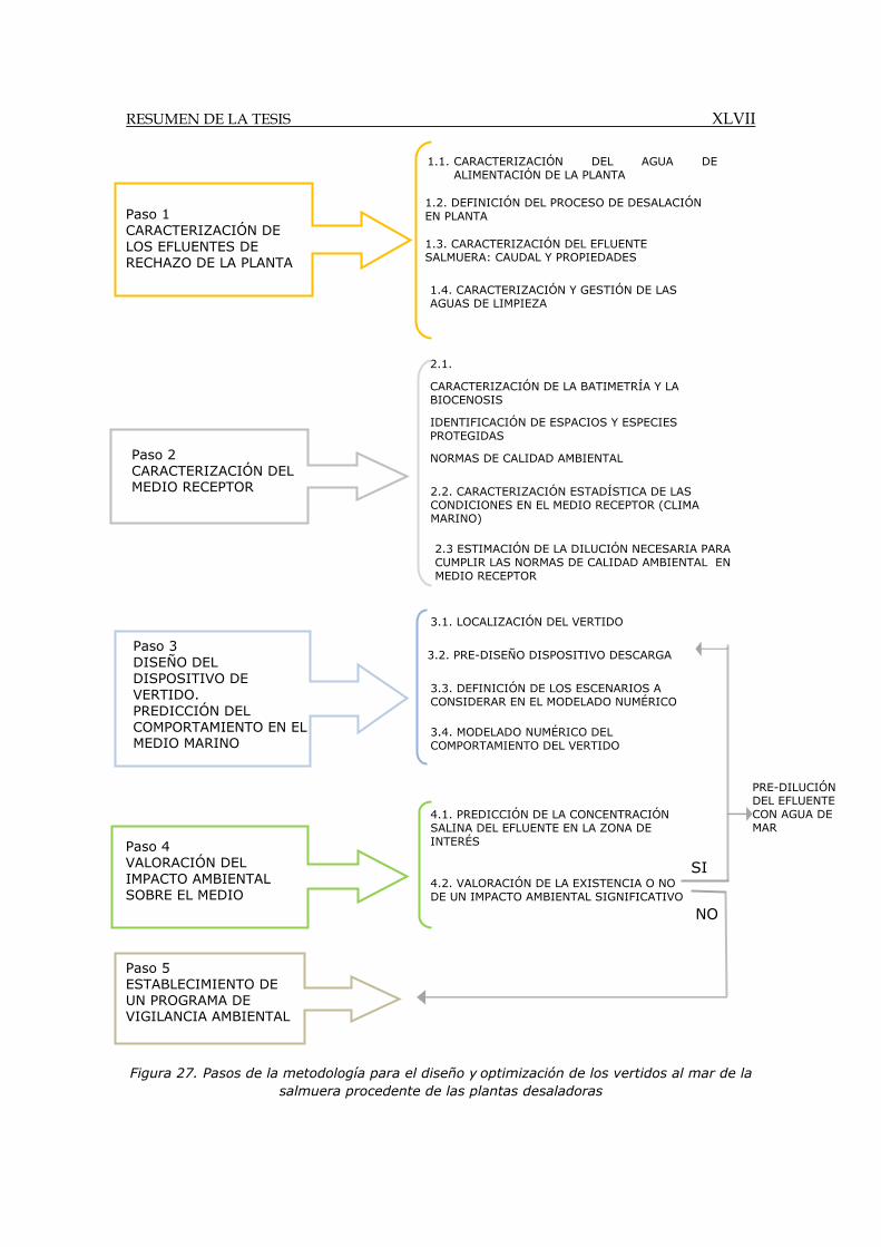
RESUMEN DE LA TESIS XLVII
Figura 27. Pasos de la metodología para el diseño y optimización de los vertidos al mar de la salmuera procedente de las plantas desaladoras
NO
2.3 ESTIMACIÓN DE LA DILUCIÓN NECESARIA PARA CUMPLIR LAS NORMAS DE CALIDAD AMBIENTAL EN MEDIO RECEPTOR
4.1. PREDICCIÓN DE LA CONCENTRACIÓN SALINA DEL EFLUENTE EN LA ZONA DE INTERÉS
4.2. VALORACIÓN DE LA EXISTENCIA O NO DE UN IMPACTO AMBIENTAL SIGNIFICATIVO
PRE-DILUCIÓN DEL EFLUENTE CON AGUA DE MAR
Paso 5 ESTABLECIMIENTO DE UN PROGRAMA DE VIGILANCIA AMBIENTAL
3.4. MODELADO NUMÉRICO DEL COMPORTAMIENTO DEL VERTIDO
2.1.
CARACTERIZACIÓN DE LA BATIMETRÍA Y LA BIOCENOSIS
IDENTIFICACIÓN DE ESPACIOS Y ESPECIES PROTEGIDAS
NORMAS DE CALIDAD AMBIENTAL Paso 2 CARACTERIZACIÓN DEL MEDIO RECEPTOR 2.2. CARACTERIZACIÓN ESTADÍSTICA DE LAS
CONDICIONES EN EL MEDIO RECEPTOR (CLIMA MARINO)
1.1. CARACTERIZACIÓN DEL AGUA DE ALIMENTACIÓN DE LA PLANTA
1.3. CARACTERIZACIÓN DEL EFLUENTE SALMUERA: CAUDAL Y PROPIEDADES
1.4. CARACTERIZACIÓN Y GESTIÓN DE LAS AGUAS DE LIMPIEZA
3.1. LOCALIZACIÓN DEL VERTIDO
Paso 3 DISEÑO DEL DISPOSITIVO DE VERTIDO. PREDICCIÓN DEL COMPORTAMIENTO EN EL MEDIO MARINO
3.3. DEFINICIÓN DE LOS ESCENARIOS A CONSIDERAR EN EL MODELADO NUMÉRICO
1.2. DEFINICIÓN DEL PROCESO DE DESALACIÓN EN PLANTA
3.2. PRE-DISEÑO DISPOSITIVO DESCARGA
Paso 1 CARACTERIZACIÓN DE LOS EFLUENTES DE RECHAZO DE LA PLANTA
Paso 4 VALORACIÓN DEL IMPACTO AMBIENTAL SOBRE EL MEDIO
SI

XLVIII RESUMEN DE LA TESIS
Paso 1. Caracterización de los efluentes de rechazo de la desalación
El primer paso se centra en caracterizar el caudal y propiedades del principal
efluente subproducto de la desalación, la salmuera, si bien también debe
considerarse también en la gestión las aguas procedentes de operaciones de
limpieza en planta. A continuación se describen los subpasos para caracterizar la
salmuera.
Paso 1.1. Caracterizar el agua de alimentación de la planta
Las propiedades de la salmuera dependen del agua de alimentación, de la
tecnología de desalación, de la tasa de conversión de la planta y de los aditivos
químicos del pre-tratamiento.
En primer lugar es necesario determinar la temperatura ( , salinidad ( y
densidad ( ) del agua de alimentación a una escala suficientemente representativa
(mensual, quincenal, etc.) y coherente con los patrones de comportamiento de
dichas variables climáticas. Se recomienda obtener dichas propiedades a partir del
análisis estadístico de series temporales de datos suficientemente larga en la zona
donde se localiza la obra de toma.
La composición y concentración de sólidos y otras sustancias en el agua de
alimentación determina el tipo y dosis de aditivos químicos a utilizar en el pre-
tratamiento.
Paso 1.2. Definir el proceso de desalación
Se define el régimen de caudales de producción en la planta ( ), el tipo de
tecnología de separación de sales y la tasa de conversión del proceso ( : ratio
entre el caudal de producción de agua desalinizada, , y el caudal de agua de
alimentación, ó ).
Paso 1.3. Caracterizar el efluente salmuera
El caudal de salmuera ( ) se obtiene a partir del caudal de producción ( ) y de la
tasa de conversión de la planta ( .
1 ó1
La concentración salina de la salmuera ( ), y la del resto de compuestos presentes
en el agua de alimentación, se calcula de manera similar.
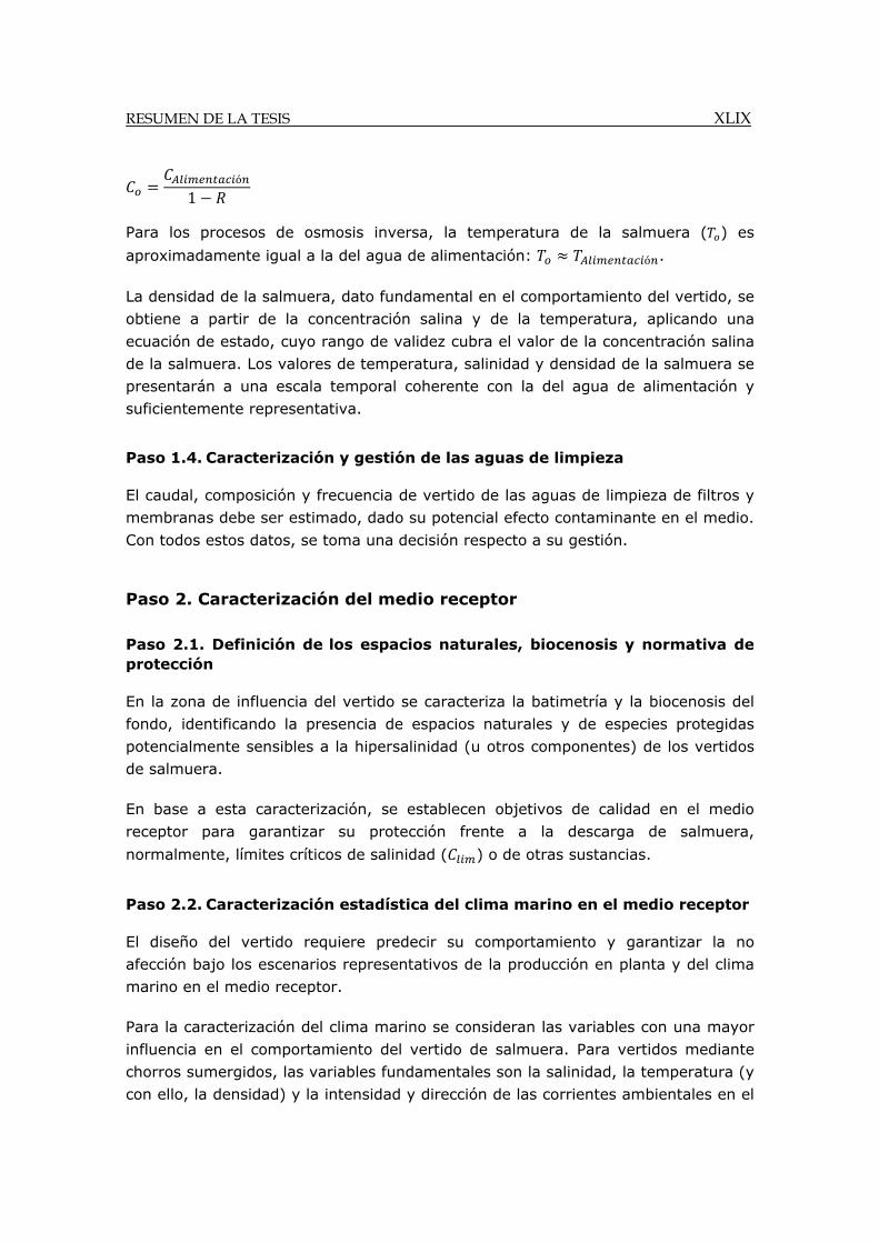
RESUMEN DE LA TESIS XLIX
ó
1
Para los procesos de osmosis inversa, la temperatura de la salmuera ( ) es
aproximadamente igual a la del agua de alimentación: ó .
La densidad de la salmuera, dato fundamental en el comportamiento del vertido, se
obtiene a partir de la concentración salina y de la temperatura, aplicando una
ecuación de estado, cuyo rango de validez cubra el valor de la concentración salina
de la salmuera. Los valores de temperatura, salinidad y densidad de la salmuera se
presentarán a una escala temporal coherente con la del agua de alimentación y
suficientemente representativa.
Paso 1.4. Caracterización y gestión de las aguas de limpieza
El caudal, composición y frecuencia de vertido de las aguas de limpieza de filtros y
membranas debe ser estimado, dado su potencial efecto contaminante en el medio.
Con todos estos datos, se toma una decisión respecto a su gestión.
Paso 2. Caracterización del medio receptor
Paso 2.1. Definición de los espacios naturales, biocenosis y normativa de protección
En la zona de influencia del vertido se caracteriza la batimetría y la biocenosis del
fondo, identificando la presencia de espacios naturales y de especies protegidas
potencialmente sensibles a la hipersalinidad (u otros componentes) de los vertidos
de salmuera.
En base a esta caracterización, se establecen objetivos de calidad en el medio
receptor para garantizar su protección frente a la descarga de salmuera,
normalmente, límites críticos de salinidad ( ) o de otras sustancias.
Paso 2.2. Caracterización estadística del clima marino en el medio receptor
El diseño del vertido requiere predecir su comportamiento y garantizar la no
afección bajo los escenarios representativos de la producción en planta y del clima
marino en el medio receptor.
Para la caracterización del clima marino se consideran las variables con una mayor
influencia en el comportamiento del vertido de salmuera. Para vertidos mediante
chorros sumergidos, las variables fundamentales son la salinidad, la temperatura (y
con ello, la densidad) y la intensidad y dirección de las corrientes ambientales en el
L RESUMEN DE LA TESIS
medio receptor. Del mismo modo que para el agua de alimentación, estas variables
se deben caracterizar a una escala adecuada para garantizar la representatividad
de las condiciones en el medio receptor. Además, debe ser coherente (y considerar
persistencias, en caso necesario) con el establecimiento de las normas de calidad o
de los límites críticos de salinidad (p.e. no superar un umbral de salinidad durante
un determinado tiempo).
Paso 2.3. Estimación de la dilución necesaria para garantizar el cumplimiento de los objetivos de calidad en el medio receptor
La dilución necesaria ( ) para no sobrepasar los límites críticos de salinidad
establecidos en el medio receptor ( ), se calcula a partir de la concentración
salina del efluente ( ), la salinidad en el medio receptor del vertido (o en la zona a
proteger) y el citado umbral crítico ( ), mediante la fórmula: .
Paso 3. Diseño del dispositivo de vertido. Predicción del comportamiento
Paso 3.1. Localización y dispositivo de vertido. Prediseño
Siempre que sea posible, la descarga de salmuera debe situarse lo más alejada
posible de espacios protegidos o zonas que albergan especies sensibles, además de
localizarse suficientemente lejos de la obra de toma. Zonas con elevada
hidrodinámica son recomendables porque incrementan la dilución del efluente.
El sistema de descarga determina el comportamiento del vertido en la región de
campo cercano. Su elección depende de diversos factores. Para caudales grandes o
vertidos en zonas sensibles siempre se recomienda utilizar emisarios submarinos
con tramo difusor de chorros múltiples.
Los parámetros de prediseño del sistema de descarga en general se establecen de
modo que se maximice la dilución La Tesis ofrece recomendaciones específicas
(ángulo de descarga entre 45º y 60º, altura mínima de la boquilla respecto al fondo
de 1 m, velocidades de descarga mayores a 4 m/s, etc.).
Paso 3.3. Definir los escenarios a considerar en el modelado del vertido
Considerando el régimen de funcionamiento de la planta desaladora y las
condiciones climáticas representativas del medio receptor, se definen los escenarios
a considerar en el modelado de predicción del comportamiento del vertido de
salmuera.
RESUMEN DE LA TESIS LI
Paso 3.4. Modelado numérico de predicción del comportamiento del vertido
El modelado numérico tiene como objetivo predecir el comportamiento del efluente
salmuera, para el sistema de descarga elegido y los escenarios representativos
seleccionados.
El primer paso en el modelado es identificar las herramientas disponibles para la
simulación y seleccionar la más adecuada para el estudio. Como alternativa a los
modelos comerciales, cuyas limitaciones ya se han descrito, se proponen las
herramientas “brIHne”. También existe la posibilidad, en caso de configuraciones
complejas, de utilizar un modelo CFD o ensayos experimentales específicos.
Seleccionado el modelo, éste se ejecuta para simular el comportamiento del vertido
bajo todos los escenarios seleccionados, obteniendo la evolución de la trayectoria y
dilución del flujo de salmuera.
Paso 4. Valoración del impacto ambiental
Para valorar el potencial impacto del vertido sobre el medio, se compara, para
todos los escenarios considerados, la dilución obtenida numéricamente de la
simulación ( ó ) con la dilución requerida para cumplir con los objetivos de
calidad establecidos para garantizar la protección del medio receptor ( ).
Si ó es previsible un impacto significativo.
Si para alguno de los escenarios se prevé la existencia de impacto significativo, se
debe modificar la localización de la descarga o los parámetros de diseño del vertido
o bien realizar una pre-dilución con agua de mar previamente a la descarga.
Paso 5. Medidas preventivas y Plan de Vigilancia Ambiental
La principal medida preventiva es diseñar el dispositivo de descarga para conseguir
los objetivos de calidad establecidos, en todos los escenarios representativos de las
condiciones en planta y de de clima marino en el medio receptor. Para garantizar la
protección del medio en la fase de explotación de la planta desaladora, se establece
un Plan de Vigilancia Ambiental y un protocolo de actuación.
En la Tesis, la metodología propuesta se aplica a un caso realista de vertido de
planta desaladora de ósmosis inversa en el Mar Mediterráneo.
LII RESUMEN DE LA TESIS
CONCLUSIONES Y CONTRIBUCIONES
La revisión de Estudios de Impacto Ambiental y de proyectos de plantas
desaladoras ha revelado carencias metodológicas y de criterios respecto a las
descargas de salmuera.
Para solventar estas carencias, en la presente Tesis se ha planteado como primer
objetivo desarrollar una metodología para el diseño de los vertidos de salmuera,
bajo la perspectiva de minimizar su potencial impacto sobre el medio marino.
Seleccionados todos los aspectos a considerar, se ha realizado una revisión de su
estado del arte, identificando los vacíos de conocimiento específicos más
relevantes. Entre éstos, se han seleccionado los relacionados con el
comportamiento del vertido y con su predicción mediante modelos numéricos, como
objeto de investigación en el marco de esta Tesis. La investigación se ha centrado
en descargas de salmuera mediante chorros sumergidos, por ser el dispositivo más
utilizado en la actualidad. De la selección de estos vacíos de conocimiento, han
nacido objetivos específicos, complementarios al desarrollo de la metodología.
El primer objetivo se ha centrado en el análisis crítico y la validación con datos
experimentales de las herramientas comerciales más utilizadas y aceptadas para
simular el comportamiento de los vertidos al mar de la salmuera (CORMIX, VISUAL
PLUMES y VISJET). El desarrollo de este objetivo se presenta en los capítulos 3 y 4
de la Tesis. La investigación ha revelado importantes limitaciones de estos modelos
y desviaciones significativas en sus resultados con respecto a datos experimentales
publicados en la literatura, especialmente en relación con la dilución del efluente,
parámetro fundamental en el diseño.
Estas desviaciones de los resultados numéricos de los modelos comerciales hacen
pensar que las hipótesis asumidas por sus aproximaciones numéricas no se ajustan
correctamente al comportamiento real del flujo simulado (en este caso, chorros
inclinados y con flotabilidad negativa). Esta suposición, unida a la escasez de
estudios publicados donde se profundice en el comportamiento de este tipo de
flujos, nos ha llevado a plantear como segundo objetivo, llevar a cabo un estudio
experimental para ahondar en los procesos que rigen el comportamiento de este
tipo de vertidos. Para la medición en los ensayos, se han utilizado técnicas ópticas
avanzadas de anemometría láser PIV (Particle Image Velocimetry) y PLIF (Planar
laser Induced Fluorescence), abarcando la región de campo cercano (chorro y capa
de esparcimiento lateral). Los ensayos experimentales llevados a cabo se describen
en el Capítulo 6 de la Tesis.
RESUMEN DE LA TESIS LIII
El análisis de los datos experimentales ha permitido describir en detalle el
comportamiento del flujo en vertidos de salmuera mediante chorros, valorando la
influencia del Número de Froude Densimétrico y del ángulo en la descarga,
parámetros fundamentales según el análisis dimensional. El estudio ha revelado
interesantes particularidades en los chorros inclinados y con flotabilidad negativa
que los alejan del comportamiento clásico de chorros neutros, invalidando algunas
de las hipótesis tradicionalmente asumidas en el modelado numérico. Un ejemplo
es la asimetría de la sección transversal del chorro denso debida a la caída de
vórtices desde el borde inferior (inestabilidad asociada a la flotabilidad negativa).
Esta asimetría hace no asumibles las hipótesis de auto-semejanza entre secciones y
perfil de tipo Gauss. El estudio del comportamiento del chorro en base al análisis de
los datos experimentales se desarrolla en los Capítulos 6 y 7 de la Tesis, mientras
que la caracterización de la spreading layer, en el Capítulo 8.
Las limitaciones y errores de predicción de los modelos comerciales, junto con la
imposibilidad de acceder a sus códigos, ha llevado a plantear el objetivo de
desarrollar nuevos modelos de simulación para vertidos de salmuera, que se ha
materializado en las herramientas “brIHne”. Estas herramientas se centran por el
momento en vertidos mediante chorros individuales y múltiples, con distinto
dominio de cálculo (campo cercano y lejano) y basadas en distintas aproximaciones
numéricas. Una ventaja de los modelos “brIhne” es su calibración con los datos
experimentales obtenidos mediante técnicas ópticas en el marco de esta Tesis, lo
que supone una mejora de su grado de ajuste a los datos experimentales y, por
tanto, de su fiabilidad en la predicción de vertidos de plantas desaladoras reales.
Estos modelos se han hecho accesibles a potenciales usuarios a través del portal
web www.brihne.ihcantabria.com. La descripción de las herramientas “brIHne” se
desarrolla en el capítulo 9 de la Tesis.
El conocimiento, recomendaciones y herramientas desarrolladas en estos objetivos
se han integrado en la metodología elaborada para el diseño de los vertidos al mar
de salmuera y la valoración de potenciales impactos sobre el medio marino. Dicha
metodología incluye los pasos secuenciales a llevar a cabo, considerando los
aspectos de influencia en el comportamiento del vertido y en su interacción con el
medio. La metodología se muestra en el Capítulo 10 de la Tesis, y se ha hecho
accesible a través del portal web: www.medvsa.es.
LIV RESUMEN DE LA TESIS
FUTURAS LÍNEAS DE INVESTIGACIÓN
Considerando los aspectos contemplados en la Guía Metodológica, las líneas de
investigación que se pueden proponer son muy diversas. A continuación se
sintetizan las más relevantes:
• Establecer objetivos de calidad en el medio receptor para especies sensibles y de
valor ecológico presentes en áreas objeto de vertidos de plantas desaladoras.
• Desarrollar una metodología para la selección de escenarios de clima marino para
vertidos de salmuera, considerando las variables más influyentes en su
comportamiento y umbrales de persistencia acordes con el establecimiento de los
límites críticos de salinidad.
• Ampliar la investigación experimental mediante técnicas ópticas a otras
configuraciones de descarga. En particular, vertidos mediante tramo difusor de
chorros múltiples y vertidos directos superficiales. Incluir condiciones de medio
receptor estático y dinámico.
• Ampliar la investigación experimental al comportamiento en la región de campo
lejano, profundizando en el comportamiento del flujo y generando una base de
datos para calibrar y validar modelos numéricos.
• Profundizar, gracias al análisis de los datos experimentales, en las ecuaciones de
gobierno para este tipo de flujo, valorando el peso de los distintos términos y
mejorando las aproximaciones para tener en cuenta comportamientos específicos,
como es el extra-ensanchamiento del borde inferior del chorro.
• Desarrollar nuevas herramientas “brIHne” para nuevas configuraciones de
descarga y condiciones del medio receptor, calibradas con datos experimentales.
• Implementar modelos avanzados, CFD, al modelado del campo cercano de
vertidos de salmuera, y modelos hidrodinámicos, para simular el comportamiento
de la pluma hipersalina característica del comportamiento en la región de campo
lejano.
• Extender las condiciones de acoplamiento campo cercano-lejano del vertido en
chorro a un caso tridimensional. Investigar estas condiciones para diferentes
configuraciones de vertido.
RESUMEN DE LA TESIS LV
Lista de Tablas
Tabla 1. Límites críticos de salinidad para distintos tipos de fanerógamas marinas.
Tabla 2. Módulos de los Software comerciales aplicables a la simulación de vertidos
de salmuera.
Tabla 3. Coeficientes de análisis dimensional propuestos por varios autores para un
vertido de chorro hiperdenso en un medio receptor en reposo.
Tabla 4. Parámetros de entrada a los modelos comerciales para su validación.
Tabla 5. Desviaciones de los modelos comerciales respecto a los datos
experimentales en la simulación de vertidos en chorro de salmuera en un medio
receptor en reposo.
Tabla 6. Desviaciones de los modelos comerciales respecto a los datos
experimentales en la simulación de vertidos en chorro de salmuera en un medio
receptor dinámico.
Tabla 7. Selección de parámetros PIV para los ensayos de caracterización del
comportamiento en campo cercano de un vertido en chorro de salmuera.
Tabla 8. Coeficientes de análisis dimensional obtenidos experimentalmente en este
trabajo.
Tabla 9. Modelos brIHne para simulación de vertidos de salmuera mediante chorro
sumergido.
LVI RESUMEN DE LA TESIS
Lista de Figuras
Figura 1. Esquema del comportamiento de un vertido de salmuera mediante chorro
sumergido.
Figura 2. Fotografía de un ensayo de vertido de salmuera en chorro en el IH
Cantabria.
Figura 3. Variables en los puntos singulares de la trayectoria de un chorro denso e
inclinado.
Figura 4. Validación de los modelos comerciales para la máxima altura del borde
superior del chorro (panel izquierdo) y la dilución en el eje en el punto de impacto
(panel derecho).
Figura 5. Esquema (panel izquierdo) y fotografía (panel derecho) de la
configuración de ensayo.
Figura 6. Principio de funcionamiento de la técnica PIV (panel superior) e
identificación del pico de desplazamiento (panel inferior).
Figura 7. Tiempos entre pulsos para la caracterización de la velocidad en el eje del
flujo en la región de campo de un vertido de salmuera mediante chorro.
Figura 8. Imagen de flujo de ensayo iluminado por el plano láser.
Figura 9. Curva de calibración PLIF.
Figura 10. Corrección de la irregularidad de luminosidad en el plano transversal.
Figura 11. Áreas del chorro en los ensayos donde los fenómenos de atenuación por
la presencia de la Rodamina 6G son significativos.
Figura 12. Análisis de convergencia de estadísticos para las velocidades medias y
turbulentas del chorro.
Figura 13. Influencia del flujo de caudal en la fuente en las hipótesis de análisis
dimensional.
RESUMEN DE LA TESIS LVII
Figura 14. Evolución de las variables (adimensionalizadas) en el eje de
concentración del chorro.
Figura 15. Evolución de las variables (adimensionalizadas) en el eje de velocidad
del chorro.
Figura 16. Validación de los datos experimentales obtenidos con datos de trabajos
previos.
Figura 17. Campos de las componentes horizontal ( ) y vertical ( ) de velocidad
media para chorros densos inclinados en la descarga 15º y 75º.
Figura 18. Campos de vorticidad en chorros densos inclinados en la descarga 15º y
75º.
Figura 19. Campos de dilución en chorros densos inclinados en la descarga 15º y
75º.
Figura 20. Campos de concentración instantánea en chorros densos inclinados 15º
y 75º.
Figura 21. Perfiles de adimensionalizados de velocidad y concentración media en un
chorro denso con inclinación en la descarga de 60º.
Figura 22. Campos hidrodinámicos de la capa de esparcimiento lateral derivada de
un chorro densos con inclinación en la descarga de 30º.
Figura 23. Campos de dilución media y de concentración instantánea en la capa de
esparcimiento lateral de un chorro con inclinación en la descarga de 30º.
Figura 24. Evolución de las variables normalizadas a lo largo de los ejes de los ejes
de concentración y velocidad el flujo en la región de campo cercano de un vertido
de salmuera en chorro.
Figura 25. Perfiles transversales adimensionalizados de velocidad y concentración
media y turbulenta en la spreading layer derivada de un chorro inclinado 30º.
Figura 26. Ejemplo de interfaz de datos de entrada del modelo brIHne-Jet-
Spreading.
Figura 27. Pasos de la metodología para el diseño y optimización de los vertidos al
mar de la salmuera procedente de las plantas desaladoras.

UNIVERSIDAD DE CANTABRIA
E.T.S. DE INGENIEROS DE CAMINOS, CANALES Y PUERTOS
Departamento de Ciencias y Técnicas del Agua y del Medio Ambiente
TESIS DOCTORAL
EXPERIMENTAL AND NUMERICAL
OPTIMIZATION OF BRINE DISCHARGES IN
THE MARINE ENVIRONMENT
Presentada por: PILAR PALOMAR HERRERO Dirigida por: ÍÑIGO J. LOSADA RODRÍGUEZ
JAVIER LÓPEZ LARA
Santander, Abril 2014


OUTLINE
Notation ............................................................................................................................................................... 1
Preface ............................................................................................................................................................... 7
Chapter 1. INTRODUCTION AND MOTIVATION ..................................................................................... 9
Summary ....................................................................................................................... 9 1.1. The need for water resources. Desalination worldwide .................................. 10 1.2. Reverse osmosis desalination technology ....................................................... 12 1.3. Desalination in Spain ....................................................................................... 14 1.4. Brine and other desalination sub-products ..................................................... 14 1.5. Behavior of brine discharges into seawaters .................................................. 16
1.5.1. Near and far field regions ................................................................................................... 16
1.5.2. Discharge configurations and efficiency ............................................................................. 16
1.5.3. Brine discharge systems in Spanish desalination plants ..................................................... 19
1.5.4. Brine discharge through submerged jets ........................................................................... 21
1.6. Impacts of brine on the marine environment ................................................. 23 1.7. Environmental impact assessment and regulation of brine discharges .......... 27 1.8. Conclusions ...................................................................................................... 28
Chapter 2. OBJECTIVES AND METHODOLOGY ..................................................................................... 31
2.1. Objectives. ....................................................................................................... 31 2.2. Methodology. ................................................................................................... 34
Chapter 3. ANALYSIS OF COMMERCIAL MODELS FOR BRINE DISCHARGES ......................... 37
Summary ..................................................................................................................... 37 3.1. Introduction .................................................................................................... 38 3.2. Modelling as a predictive tool .......................................................................... 40
3.2.1. Models based on the dimensional analysis of the relevant processes ............................... 40
3.2.2. Models based on the integration of differential equations ............................................... 42
3.2.3. Computational Fluid Dynamics (CFDs) models ................................................................... 43
3.3. Critical assessment of CORMIX, VISUAL PLUMES and VISJET softwares for brine discharge modelling ........................................................................................... 43
3.3.1. Software general description ............................................................................................. 43
3.3.2. CORMIX1 and CORMIX2: Commercial models based on dimensional analysis .................. 47
3.3.3. CORJET, UM3 and JETLAG: Commercial models based on the integration of differential equations .......................................................................................................................................... 56
3.4. Range of actual and recommended values for input data ............................... 60 3.5. Conclusions ...................................................................................................... 63
Chapter 4. VALIDATION OF COMMERCIAL TOOLS FOR BRINE DISCHARGES ....................... 67
Summary ..................................................................................................................... 67 4.1. Introduction .................................................................................................... 68 4.2. Experimental data selected for commercial models validation....................... 68
4.2.1. Experimental data for an inclined dense jet discharged into a stagnant environment ..... 69
4.2.2. Experimental data for an inclined dense jet discharged into a dynamic environment ...... 73
4.3. CORMIX, VISUAL PLUMES and VISJET software validation ............................ 76 4.3.1. Validation for an inclined dense jet into a stagnant environment ..................................... 77
4.3.2. Validation for an inclined dense jet into a dynamic environment ..................................... 87
4.4. Conclusions ...................................................................................................... 95
Chapter 5. EXPERIMENTAL STUDY OF BRINE JET DISCHARGES USING LASER ANEMOMETRY ............................................................................................................................................................ 99
Summary ..................................................................................................................... 99 5.1. Introduction .................................................................................................. 100 5.2. Experimental setup ........................................................................................ 101 5.3. Instrumentation ............................................................................................ 105 5.4. Velocity measurement by PIV ....................................................................... 108
5.4.1. Brief PIV technique description ........................................................................................ 108
5.4.2. Selection of the seeding tracer PIV particles and density within the flow ....................... 110
5.4.3. Selection of separation between pulses ........................................................................... 112
5.4.4. Size of interrogation windows .......................................................................................... 116
5.4.5. Cross‐correlation function ................................................................................................ 117
5.4.6. Summary of PIV parameter .............................................................................................. 118
5.5. Concentration measurement by PLIF ............................................................ 119 5.5.1. PLIF technique brief description ....................................................................................... 119
5.5.2. Dye tracer type selection and photobleaching ................................................................. 120
5.5.3. PLIF image corrections. Attenuation coefficients ............................................................. 124
5.5.4. Dye tracer concentration .................................................................................................. 130
5.5.5. PLIF calibration ................................................................................................................. 131
5.5.6. Summary of PLIF parameter ............................................................................................. 134
5.6. Timing of the combined PIV-PLIF system ..................................................... 134 5.7. Quality control. Number of PLIF and PIV images .......................................... 135
5.7.1. Flow stationary state ........................................................................................................ 135
5.7.2. Convergence of statistics .................................................................................................. 137
5.8. Conclusions .................................................................................................... 141
Chapter 6. BRINE JET DIMENSIONAL ANALYSIS AND LONGITUDINAL PROFILE BASED ON THE EXPERIMENTAL DATA ANALYSIS ................................................................................... 145
Summary ................................................................................................................... 145 6.1. Introduction .................................................................................................. 146 6.2. Experimental test description ....................................................................... 147
6.2.1. Tests and prototype similarities ....................................................................................... 147

6.2.2. Design of the experiments ................................................................................................ 149
6.2.3. Case study ......................................................................................................................... 150
6.3. Jet centerline and dimensional analysis ........................................................ 152 6.3.1. Velocity and concentration centerlines ............................................................................ 152
6.3.2. Jet path variables .............................................................................................................. 154
6.3.3. Influence of the Densimetric Froude number on the jet behavior .................................. 156
6.3.4. Dimensional analysis formulas for negatively buoyant jets ............................................. 159
6.4. Jet longitudinal profiles ................................................................................. 160 6.4.1. Evolution of variables along the jet concentration centerline ......................................... 160
6.4.2. Evolution of hydrodynamic variables along the jet velocity centerline ........................... 162
6.4.3. Experimental coefficients at singular points .................................................................... 164
6.5. Validation with data from other authors ....................................................... 168 6.6. Conclusions .................................................................................................... 174
Chapter 7. BRINE JET FLOW FIEDS AND TRANSVERSE PROFILES BASED ON THE EXPERIMENTAL DATA ANALYSIS .................................................................................................................... 177
Summary ................................................................................................................... 177 7.1. Introduction .................................................................................................. 178
7.1.1. Case study ......................................................................................................................... 179
7.2. Description of the flow-fields ........................................................................ 180 7.2.1. Time averaged horizontal and vertical velocity fields and vorticity ................................. 180
7.2.2. Dilution fields .................................................................................................................... 189
7.3. Cross-section analysis ................................................................................... 192 7.3.1. Velocity and concentration profile evolution along the jet path ..................................... 193
7.3.2. Nondimensional transverse profiles. Assessment of the self similarity and Gaussian profile hypothesis ....................................................................................................................................... 198
7.3.3. Turbulent variables profiles .............................................................................................. 207
7.4. Conclusions .................................................................................................... 210
Chapter 8. BRINE SPREADING LAYER CHARACTERIZATION BASED ON THE ANALYSIS OF EXPERIMENTAL DATA ............................................................................................................. 213
Summary ................................................................................................................... 213 8.1. Introduction .................................................................................................. 214
8.1.1. General behavior of an inclined dense jet discharge in the near field region .................. 216
8.2. Experimental test .......................................................................................... 217 8.2.1. Particular features of PIV and PLIF tests for the spreading layer ..................................... 217
8.2.2. Design of the experiments. ............................................................................................... 218
8.2.3. Case study ......................................................................................................................... 220
8.3. Flow-fields ..................................................................................................... 220 8.3.1. Averaged and turbulent velocity fields ............................................................................. 221
8.3.2. Dilution fields .................................................................................................................... 224
8.3.3. Variable fluctuation relative to average value ................................................................. 227
8.4. Dimensional analysis of spreading layer variables........................................ 229
8.4.1. Defining variables and formulas ....................................................................................... 229
8.4.2. Velocity and concentration centerlines of the spreading layer ........................................ 230
8.4.3. Evolution of variables along the spreading layer centerline. Longitudinal profile ........... 232
8.4.4. Dimensional analysis coefficients ..................................................................................... 236
8.5. Cross-section analysis ................................................................................... 238 8.5.1. Velocity and concentration cross‐section evolution along the spreading layer ............... 238
8.5.2. Nondimensional transverse profiles. Self similarity ......................................................... 242
8.6. Validation of PIV-PLIF results with other experimental data ....................... 244 8.7. Conclusions .................................................................................................... 245
Chapter 9. NEW “BRIHNE” NUMERICAL TOOLS TO SIMULATE BRINE DISCHARGES ...... 249
Summary ................................................................................................................... 249 9.1. Introduction .................................................................................................. 250
9.1.1. Governing equations ........................................................................................................ 250
9.1.2. Model types according to the mathematical approach ................................................... 252
9.2. BrIHne SIMULATION TOOLS ......................................................................... 253 9.2.1. Description and types ....................................................................................................... 253
9.3. BrIHne-Jet ..................................................................................................... 256 9.3.1. Simulation scheme and scope .......................................................................................... 256
9.3.2. Governing equations approach ........................................................................................ 257
9.3.3. Technical Specifications .................................................................................................... 262
9.3.4. Input data ......................................................................................................................... 264
9.3.5. Model results .................................................................................................................... 264
9.4. BrIHne-Jet-Spreading ................................................................................... 265 9.4.1. Simulation scheme and scope .......................................................................................... 265
9.4.2. Governing equations approach ........................................................................................ 266
9.4.3. Transverse profiles ........................................................................................................... 268
9.4.4. Coupling conditions for a far field model ......................................................................... 273
9.4.5. Technical specifications .................................................................................................... 274
9.4.6. Input data ......................................................................................................................... 277
9.4.7. Model results .................................................................................................................... 277
9.4.8. Calibration ........................................................................................................................ 278
9.4.9. Validation with experimental data from various authors ................................................ 280
9.5. BrIHne-Jet-Plume2D ..................................................................................... 283 9.5.1. Simulation scheme and scope .......................................................................................... 283
9.5.2. Governing equations approach ........................................................................................ 284
9.5.3. Technical specifications .................................................................................................... 289
9.5.4. Input data ......................................................................................................................... 292
9.5.5. Results .............................................................................................................................. 292
9.6. A web based application for end-users ......................................................... 293 9.7. Conclusions .................................................................................................... 295

Chapter 10. DEVELOPMENT OF A METHODOLOGY TO DESIGN BRINE DISCHARGES ........ 297
Summary ................................................................................................................... 297 10.1. Introduction .................................................................................................. 298 10.2. Methodology steps ........................................................................................ 299
10.2.1. Characterization of brine and other desalination sub‐products ...................................... 302
10.2.2. Characterization of the marine environment and climate ............................................... 303
10.2.3. Design of brine discharge. Modeling and prediction of the brine behavior under different scenarios ......................................................................................................................................... 305
10.2.4. Environmental impact assessment ................................................................................... 308
10.3. Numerical tools to simulate brine discharges behavior ................................ 309 10.3.1. Commercial models .......................................................................................................... 309
10.3.2. BrIHne online simulation tools ......................................................................................... 310
10.4. Mediterranean marine climate atlas for brine discharges ............................. 311 10.5. Application of the methodology to a real case .............................................. 316
10.5.1. Characterization of brine and other sub‐products ........................................................... 317
10.5.2. Characterization of the environment and the marine climate ......................................... 319
10.5.3. Design of the brine discharge. Modeling and prediction of the brine behavior under different scenarios .......................................................................................................................... 324
10.5.4. Marine environmental impact assessment ...................................................................... 331
10.6. Conclusions .................................................................................................... 331
Chapter 11. CONCLUSIONS AND FUTURE RESEARCH ...................................................................... 333
11.1 Conclusions .................................................................................................... 333 11.2 Future Research ............................................................................................ 336
REFERENCES .......................................................................................................................................................... 339
LIST OF TABLES ....................................................................................................................................................... 353
LIST OF FIGURES ...................................................................................................................................................... 357

NOTATION 1
Notation
NOTATION
: Jet radius (radial distance for which concentration is 50% and velocity is 37% of
those of the centerline).
: Plume width.
: Density fraction term.
: Radial distance from the centerline corresponding to 25% of centerline
concentration.
: Radial distance from the centerline corresponding to 14% of centerline velocity.
: Jet radius the centerline peak point (corresponding to the jet upper boundary).
: Jet radius at the return point (corresponding to the jet upper boundary).
: Instantaneous concentration value.
: Ensemble averaged concentration.
: Turbulent concentration (fluctuation).
: Ambient salinity.
: Effluent salinity concentration.
: Centerline concentration (cross-section maximum concentration).
: Coefficient of drag.
: Rhodamine concentration in the experimental test.
: Port diameter.
: Entrainment term.

2 NOTATION
: Densimetric Froude number.
: Initial Densimetric Froude number.
: Drag Force.
: Reduced gravity.
: Average depth at discharge point.
: Port height.
: Kinematic buoyancy flux.
: Initial kinematic buoyancy flux.
: Diffuser length.
: Axis length from the nozzle to the centerline peak point.
:Axis length from the nozzle to the return point.
: Centerline length from the nozzle to the end of the spreading layer.
: Momentum-Buoyancy length scale.
: Flux-momentum length scale.
: Bottom slope.
: Kinematic momentum flux.
: Initial kinematic momentum flux.
: Number of PIV and PLIF images considered for the analysis.
: Number of ports.
: Brine effluent flow rate. Kinematic mass flux.
: Kinematic mass flux.
: Kinematic flux of contaminant mass.

NOTATION 3
: Jet radius (radial distance for which concentration is 25% and velocity is 7% of
those of the centerline. √2 ).
: Jet radius (radial distance for which concentration is 6% and velocity is 2% of
those of the centerline. 2 ).
: Reynolds Number.
: Richardson Number.
: Centerline length from the nozzle to the point of interest.
: Dilution rate.
: Fluorescence level measured by the PLIF camera.
: Centerline dilution.
: Critical salinity limit or threshold.
: Minimum centerline dilution at the centerline peak point.
: Centerline dilution at the impact point.
: Centerline dilution at the return point.
: Centerline (minimum) dilution at the end of the spreading layer.
: Spacing between ports or nozzle spacing.
: Ambient fluid temperature.
: Brine effluent temperature.
: Instantaneous horizontal velocity value.
: Instantaneous vertical velocity value.
: Ambient velocity.
: Initial discharge velocity.
: Ensemble averaged velocity.
: Turbulent component of velocity (fluctuation).

4 NOTATION
: Centerline velocity (cross-section maximum velocity).
: Horizontal ensemble averaged velocity.
: Horizontal turbulent velocity (fluctuation).
: Vertical ensemble averaged velocity.
: Vertical turbulent velocity (fluctuation).
: Ambient crossflow velocity ( ) relative to the jet discharge velocity ( ), ⁄ .
: Centerline velocity at the end of the spreading layer.
: Ensemble averaged planar vorticity.
: Horizontal location of the centerline peak.
: Horizontal location of the impact point.
: Horizontal location of the return point.
: Horizontal location of the end of the spreading layer (horizontal distance from
the nozzle to the end of the spreading layer).
: Plume thickness.
: Height of the centerline from the bottom at the end of the spreading layer.
: Spreading layer thickness at the end of the spreading layer.
: Vertical location of the centerline peak.
: Maximum rise height (jet upper edge).
/ : Vertical coordinate (Z) value at which velocity decreases from the centerline
(maximum) value to half this maximum value (i.e. height from the bottom where
velocity is 50% of that at the centerline).
: Jet discharge angle (vertical angle with respect to the bottom).
: Horizontal angle between jet and current.
: Angle of crossflow to the vertical plane containing the nozzle axis, 180° .

NOTATION 5
: Dispersion ratio.
, , , : Empirical coefficients of the jet flow asymptotic states.
: Pure jet coefficient.
: Pure plume coefficient.
: Pure wake coefficient.
: Advected plume coefficient.
: Horizontal angle between the jet centerline and the diffuser.
: Angle between diffuser line and ambient current.
: Eddy viscosity.
: Fluid dynamic viscosity of the fluid.
: Turbulent diffusion coefficient.
“c” suscript refers to variables at the centerline.

6 NOTATION

PREFACE 7
Preface
PREFACE The study of the current situation of brine discharges and the assessment of its
potential impact on the marine environment have required the review of the State
of the Art of various and very different disciplines related to technical aspects of
desalination processes, environmental regulation, biological effects on marine
ecosystems, brine discharge modeling, marine climate affecting brine discharges,
etc. The summary of this review carried out as the first step to establish the goals
of the present work is shown in Chapter 1.
Moreover, the thesis objectives cover a wide range of different themes, such as
critical review and validation of commercial simulation models, model scale
experiments, fluid mechanics to analyze the brine flow behavior and methodological
guidelines. Due to this diversity of subjects, it has been considered that a general
State of the Art does not make much sense in this Thesis, being preferable to
elaborate a specific and detailed State of the Art for each of these issues, which are
presented in each chapter of the present document.
The chapters are self-contained, corresponding to independent scientific articles
that have been already published or are currently in preparation. The notation and
references from all chapters have been compiled and displayed at the beginning
and at the end of the Thesis, respectively.

8 PREFACE
CHAPTER 1: INTRODUCTION AND MOTIVATION 9
Chapter 1. INTRODUCTION AND MOTIVATION
Chapter 1 INTRODUCTION AND MOTIVATION
Summary
This chapter describes the background and present situation of brine discharges
from desalination plants, which have motivated the development of this Thesis,
according to the main needs detected.
Desalination, as a fundamental alternative to conventional water sources in some
regions, has exponentially increased in the last decades. In Spain, this increase
stands out in the Mediterranean region, where the high water demand for irrigation
and tourist areas cannot be supplied by conventional water sources.
The rising of desalinated water production implies an increase of the volume of
brine (main desalination sub-product) discharged into the sea. In seawater reverse
osmosis plants, brine is a hypersaline effluent, having a higher density than
seawaters. Consequently, it has negative buoyancy when discharged into the sea.
Previous works have evidenced the existence of negative effects of brine on some
marine ecosystems. In the Mediterranean Sea, the endemic seagrass Posidonia
oceanica, with high ecological value and protected by European regulation, is an
example of brine-sensitive species, which must be protected against desalination
plant discharges.
Despite this evidence of potential negative impacts, currently there is no legislation
in place in Europe or Spain regulating brine discharges, establishing emission
thresholds or water quality standards related to this effluent. Furthermore, the

10 CHAPTER 1: INTRODUCTION AND MOTIVATION
Environmental Assessment of the largest and most recent Spanish desalination
plants, together with the review of Environmental Impact Studies (EIS) of older
desalination plants, have revealed important knowledge and criteria shortcomings
and a lack of methodologies related to the design of brine discharges and the
prediction of its behavior into the sea. This leads to significant uncertainties in the
environmental evaluation of this type of discharges.
Considering these statements, the present Thesis arises with the goal of improving
the design of brine discharges in order to minimize the environmental impacts on
the marine environment. However, the review of the State of the Art of the main
aspects to consider in the design brine discharges has evidenced the existence of
scientific knowledge gaps and the need for specific tools required for a rigorous
application of the methodology. Therefore, various additional objectives have been
set out in the present Thesis as will be shown later.
1.1. The need for water resources. Desalination worldwide
The global water demand is increasing exponentially due to the development of
demanding populations and economic activities, such as agriculture, industry or
tourism.
An effective water policy must consider appropriate demand management
strategies, as well as the recovery of costs for water services, education for water
saving practices and full implementation and enforcement of environmental
legislation, in combination with research and investment in new alternative supply
options. Alternative water sources such as water recycling, water reuse and
desalination are very important tools in the future water balance between water
supply and demand, and therefore in guaranteeing an extended availability of this
resource.
Forty-one percent of the world population (2.300 million inhabitants) lives in areas
with a marked water deficit and it is expected that by the year 2025 this amount
will reach 3.500 million. Considering that almost one quarter of the world's
population lives less than 25 km from the coast, seawater could become one of the
main sources of freshwater in the near future. Consequently, seawater desalination
has gained importance in coastal countries where conventional water sources are
insufficient or over-exploited.
Desalination is any of the several processes involved in removing dissolved
minerals (especially salt) from seawater, brackish water, or treated wastewater. It

CHAPTER 1: INTRODUCTION AND MOTIVATION 11
is a rainfall independent inexhaustible source of water, which generates a high
quality product and guarantees demand supply.
According to the 20th International Desalination Association (IDA) Worldwide
Desalting Plant Inventory, the production capacity of all desalination plants
worldwide was around 44 million cubic meters per day (Mm³/day) by the end of
2006, and is expected to more than double by 2015, Lattemann et al. (2010).
Regarding location, 6% of the plants are in the Asian Pacific region, 7% in America,
10% in Europe and 77% in the Middle East and North Africa. The six countries with
the highest production capacity of desalinated water are: Saudi Arabia (11
Mm³/day), United Arab Emirates (8.2 Mm³/day), United States (8 Mm³/day), Spain
(5.2 Mm³/day), Kuwait (2.8 Mm³/day) and Algeria (2.6 Mm³/day). Currently, the
largest desalination plant in the world is in Ashkelon (Israel), with a 330.000
m³/day production capacity, supplying water to 1.200.000 people. The second
largest one is Torrevieja (Spain) desalination plant, with a production capacity of
240.000 m³/day.
To illustrate that issue, Figure 1.1 shows a map with the highest desalination
production in the world.
Figure 1.1. Major desalted water producing countries in the world (source: Lattemann et al. 2010)
12 CHAPTER 1: INTRODUCTION AND MOTIVATION
1.2. Reverse osmosis desalination technology
Several technologies have been implemented for salt separation, being the most
important thermal processes and membrane technologies.
In thermal processes water is heated until it evaporates, and salts are separated.
Subsequently, water is condensed to produce potable water. The most used of
these techniques is the Multi-Stage Flash evaporation (MSF).
In membrane desalination, salt water passes through special membranes, which
retain the hypersaline effluent and produce freshwater. There are two main types:
Electrodialysis Membranes (ED), in which water supplies are kept under pressure to
retain the salts by applying an electrical potential and Reverse Osmosis (RO)
Membranes.
Thermal processes have significantly higher energy consumption, what justifies that
most of the MSF plants operate in oil-producing countries. RO is more common
worldwide, due to its lower energy consumption and its higher flexibility with
respect to distillation technologies.
Currently, RO represents 59% of the desalinated water production worldwide faced
to 27% obtained by Multi -Stage Flash distillation plants (MSF), which is the second
most used technology, DesalData (2010).
SWRO (seawater reverse osmosis) is nowadays and is expected to be also in the
future the most important desalination technology worldwide. Moreover, almost the
whole desalinated water flow rate in Spain comes from Reverse Osmosis plants. For
these reasons, the present Thesis focuses on this technique, in particular on the
management of the brine sub-products generated, as explained in the following
sections.
Reverse osmosis is a process in which seawater passes through permeable
membranes under high pressure. The natural osmosis process is reversed and while
the semi-permeable membranes retain the salts, they allow the water molecules to
pass through, obtaining freshwater and a brine effluent waste product.
Feed seawater in reverse osmosis is pre-treated to remove particles (sand, shells or
seaweed), which otherwise would clog the membranes, including screening,
sedimentation, filtering and the addition of chemical additives to seawater. After
pre-treatment, the operational process includes: seawater intake and inlet; pre-
treatment; high pressure pumping system; reverse osmosis membranes; outlet for
discharge; desalinated water post-treatment and distribution system.
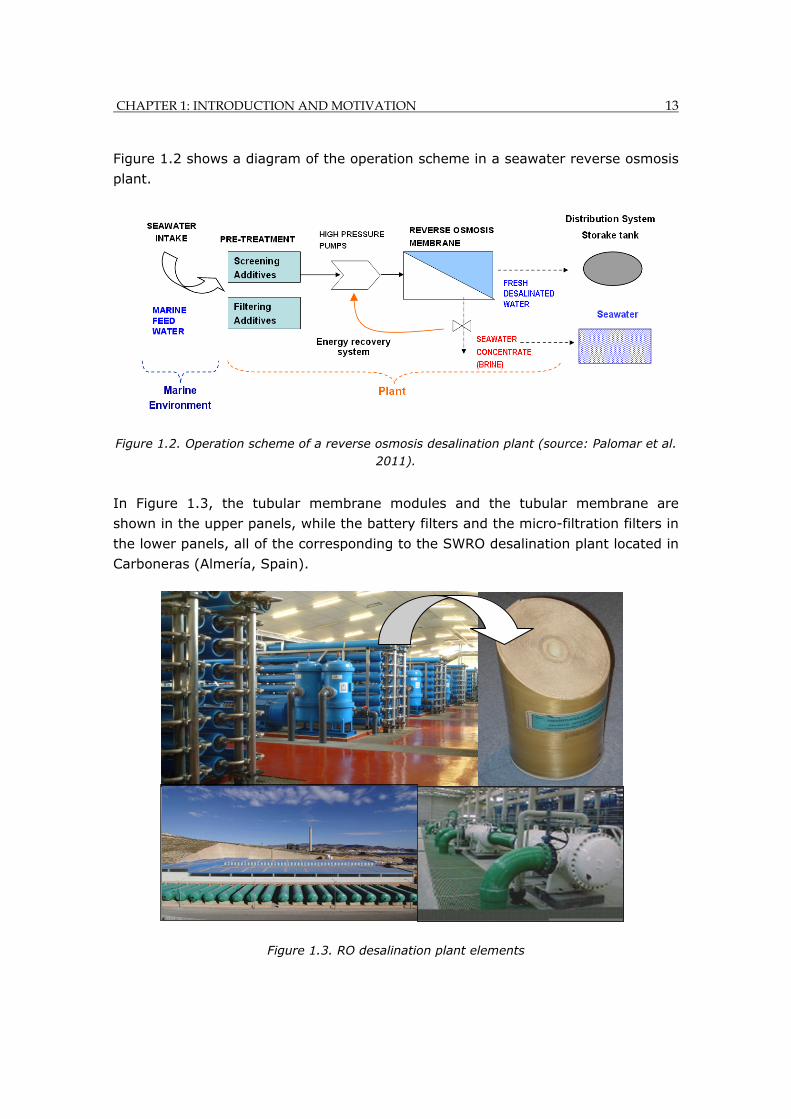
CHAPTER 1: INTRODUCTION AND MOTIVATION 13
Figure 1.2 shows a diagram of the operation scheme in a seawater reverse osmosis
plant.
Figure 1.2. Operation scheme of a reverse osmosis desalination plant (source: Palomar et al. 2011).
In Figure 1.3, the tubular membrane modules and the tubular membrane are
shown in the upper panels, while the battery filters and the micro-filtration filters in
the lower panels, all of the corresponding to the SWRO desalination plant located in
Carboneras (Almería, Spain).
Figure 1.3. RO desalination plant elements
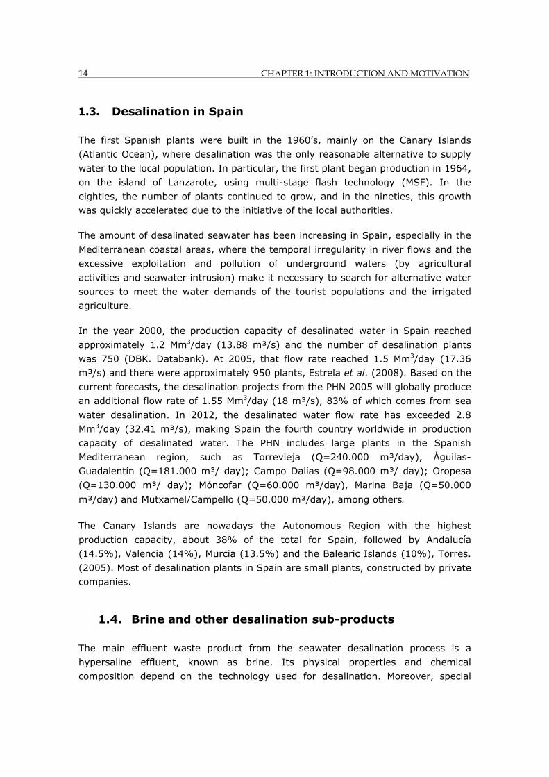
14 CHAPTER 1: INTRODUCTION AND MOTIVATION
1.3. Desalination in Spain
The first Spanish plants were built in the 1960’s, mainly on the Canary Islands
(Atlantic Ocean), where desalination was the only reasonable alternative to supply
water to the local population. In particular, the first plant began production in 1964,
on the island of Lanzarote, using multi-stage flash technology (MSF). In the
eighties, the number of plants continued to grow, and in the nineties, this growth
was quickly accelerated due to the initiative of the local authorities.
The amount of desalinated seawater has been increasing in Spain, especially in the
Mediterranean coastal areas, where the temporal irregularity in river flows and the
excessive exploitation and pollution of underground waters (by agricultural
activities and seawater intrusion) make it necessary to search for alternative water
sources to meet the water demands of the tourist populations and the irrigated
agriculture.
In the year 2000, the production capacity of desalinated water in Spain reached
approximately 1.2 Mm3/day (13.88 m³/s) and the number of desalination plants
was 750 (DBK. Databank). At 2005, that flow rate reached 1.5 Mm3/day (17.36
m³/s) and there were approximately 950 plants, Estrela et al. (2008). Based on the
current forecasts, the desalination projects from the PHN 2005 will globally produce
an additional flow rate of 1.55 Mm3/day (18 m³/s), 83% of which comes from sea
water desalination. In 2012, the desalinated water flow rate has exceeded 2.8
Mm3/day (32.41 m³/s), making Spain the fourth country worldwide in production
capacity of desalinated water. The PHN includes large plants in the Spanish
Mediterranean region, such as Torrevieja (Q=240.000 m³/day), Águilas-
Guadalentín (Q=181.000 m³/ day); Campo Dalías (Q=98.000 m³/ day); Oropesa
(Q=130.000 m³/ day); Móncofar (Q=60.000 m³/day), Marina Baja (Q=50.000
m³/day) and Mutxamel/Campello (Q=50.000 m³/day), among others.
The Canary Islands are nowadays the Autonomous Region with the highest
production capacity, about 38% of the total for Spain, followed by Andalucía
(14.5%), Valencia (14%), Murcia (13.5%) and the Balearic Islands (10%), Torres.
(2005). Most of desalination plants in Spain are small plants, constructed by private
companies.
1.4. Brine and other desalination sub-products
The main effluent waste product from the seawater desalination process is a
hypersaline effluent, known as brine. Its physical properties and chemical
composition depend on the technology used for desalination. Moreover, special
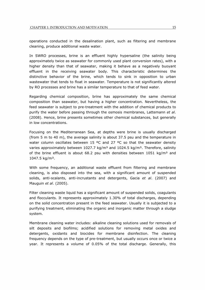
CHAPTER 1: INTRODUCTION AND MOTIVATION 15
operations conducted in the desalination plant, such as filtering and membrane
cleaning, produce additional waste water.
In SWRO processes, brine is an effluent highly hypersaline (the salinity being
approximately twice as seawater for commonly used plant conversion rates), with a
higher density than that of seawater, making it behave as a negatively buoyant
effluent in the receiving seawater body. This characteristic determines the
distinctive behavior of the brine, which tends to sink in opposition to urban
wastewater that tends to float in seawater. Temperature is not significantly altered
by RO processes and brine has a similar temperature to that of feed water.
Regarding chemical composition, brine has approximately the same chemical
composition than seawater, but having a higher concentration. Nevertheless, the
feed seawater is subject to pre-treatment with the addition of chemical products to
purify the water before passing through the osmosis membranes, Lattemann et al.
(2008). Hence, brine presents sometimes other chemical substances, but generally
in low concentrations.
Focusing on the Mediterranean Sea, at depths were brine is usually discharged
(from 5 m to 40 m), the average salinity is about 37.5 psu and the temperature in
water column oscillates between 15 ºC and 27 ºC so that the seawater density
varies approximately between 1027.7 kg/m³ and 1024.5 kg/m³. Therefore, salinity
of the brine effluent is about 68.2 psu with densities between 1051 kg/m³ and
1047.5 kg/m³.
With some frequency, an additional waste effluent from filtering and membrane
cleaning, is also disposed into the sea, with a significant amount of suspended
solids, anti-scalants, anti-incrustants and detergents, Gacia et al. (2007) and
Mauguin et al. (2005).
Filter cleaning waste liquid has a significant amount of suspended solids, coagulants
and flocculants. It represents approximately 1.30% of total discharges, depending
on the solid concentration present in the feed seawater. Usually it is subjected to a
purifying treatment, eliminating the organic and inorganic matter through a sludge
system.
Membrane cleaning water includes: alkaline cleaning solutions used for removals of
silt deposits and biofilms; acidified solutions for removing metal oxides and
detergents, oxidants and biocides for membrane disinfection. The cleaning
frequency depends on the type of pre-treatment, but usually occurs once or twice a
year. It represents a volume of 0.05% of the total discharge. Generally, this
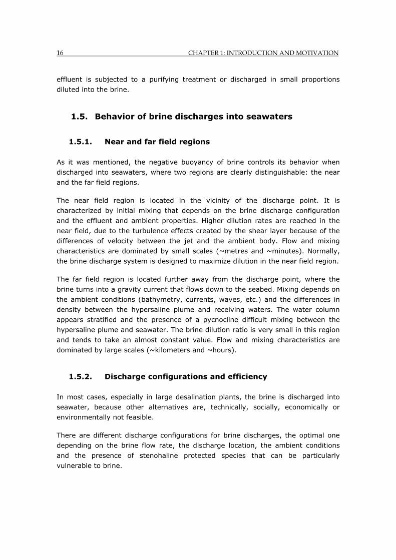
16 CHAPTER 1: INTRODUCTION AND MOTIVATION
effluent is subjected to a purifying treatment or discharged in small proportions
diluted into the brine.
1.5. Behavior of brine discharges into seawaters
1.5.1. Near and far field regions
As it was mentioned, the negative buoyancy of brine controls its behavior when
discharged into seawaters, where two regions are clearly distinguishable: the near
and the far field regions.
The near field region is located in the vicinity of the discharge point. It is
characterized by initial mixing that depends on the brine discharge configuration
and the effluent and ambient properties. Higher dilution rates are reached in the
near field, due to the turbulence effects created by the shear layer because of the
differences of velocity between the jet and the ambient body. Flow and mixing
characteristics are dominated by small scales (~metres and ~minutes). Normally,
the brine discharge system is designed to maximize dilution in the near field region.
The far field region is located further away from the discharge point, where the
brine turns into a gravity current that flows down to the seabed. Mixing depends on
the ambient conditions (bathymetry, currents, waves, etc.) and the differences in
density between the hypersaline plume and receiving waters. The water column
appears stratified and the presence of a pycnocline difficult mixing between the
hypersaline plume and seawater. The brine dilution ratio is very small in this region
and tends to take an almost constant value. Flow and mixing characteristics are
dominated by large scales (~kilometers and ~hours).
1.5.2. Discharge configurations and efficiency
In most cases, especially in large desalination plants, the brine is discharged into
seawater, because other alternatives are, technically, socially, economically or
environmentally not feasible.
There are different discharge configurations for brine discharges, the optimal one
depending on the brine flow rate, the discharge location, the ambient conditions
and the presence of stenohaline protected species that can be particularly
vulnerable to brine.
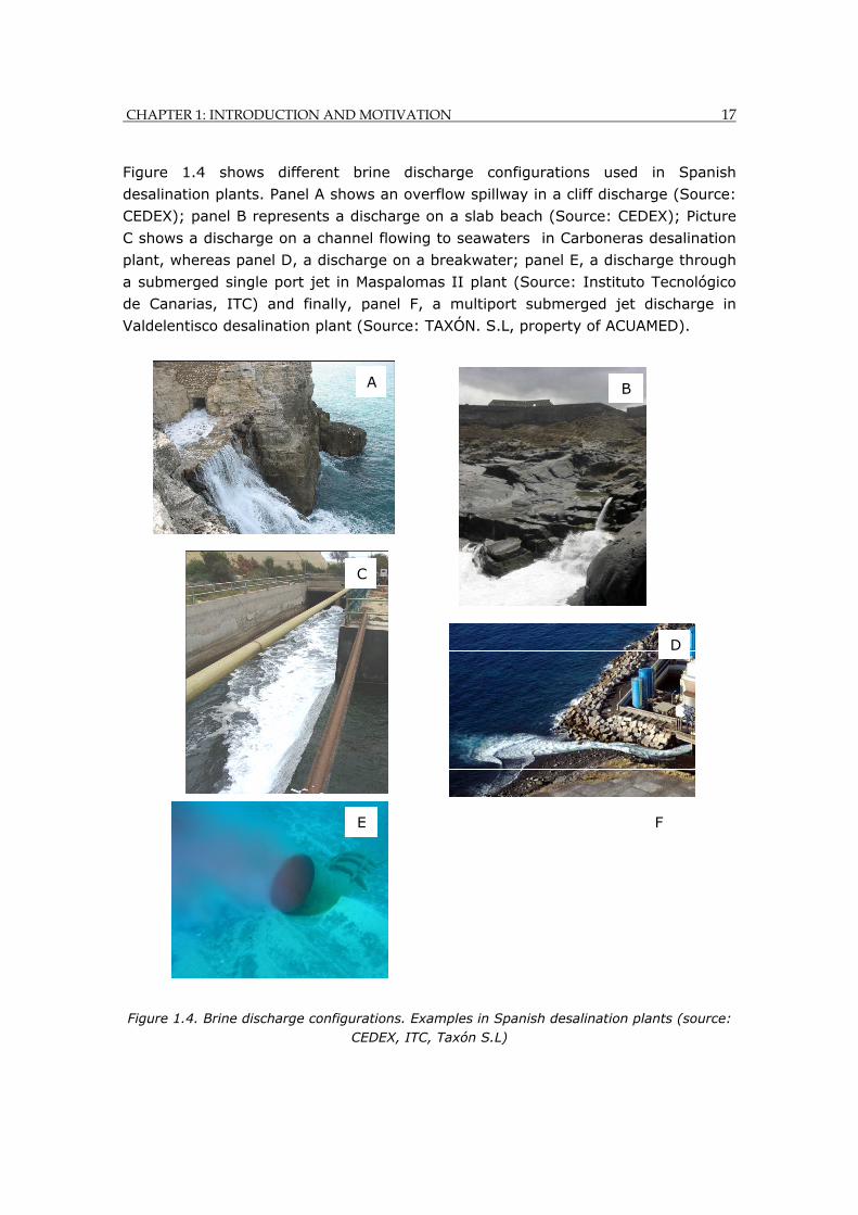
CHAPTER 1: INTRODUCTION AND MOTIVATION 17
Figure 1.4 shows different brine discharge configurations used in Spanish
desalination plants. Panel A shows an overflow spillway in a cliff discharge (Source:
CEDEX); panel B represents a discharge on a slab beach (Source: CEDEX); Picture
C shows a discharge on a channel flowing to seawaters in Carboneras desalination
plant, whereas panel D, a discharge on a breakwater; panel E, a discharge through
a submerged single port jet in Maspalomas II plant (Source: Instituto Tecnológico
de Canarias, ITC) and finally, panel F, a multiport submerged jet discharge in
Valdelentisco desalination plant (Source: TAXÓN. S.L, property of ACUAMED).
Figure 1.4. Brine discharge configurations. Examples in Spanish desalination plants (source: CEDEX, ITC, Taxón S.L)
A B
C
D
E F
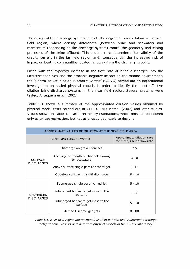
18 CHAPTER 1: INTRODUCTION AND MOTIVATION
The design of the discharge system controls the degree of brine dilution in the near
field region, where density differences (between brine and seawater) and
momentum (depending on the discharge system) control the geometry and mixing
processes of the brine effluent. This dilution rate determines the salinity of the
gravity current in the far field region and, consequently, the increasing risk of
impact on benthic communities located far away from the discharging point.
Faced with the expected increase in the flow rate of brine discharged into the
Mediterranean Sea and the probable negative impact on the marine environment,
the “Centro de Estudios de Puertos y Costas” (CEPYC) carried out an experimental
investigation on scaled physical models in order to identify the most effective
dilution brine discharge systems in the near field region. Several systems were
tested, Antequera et al. (2001).
Table 1.1 shows a summary of the approximated dilution values obtained by
physical model tests carried out at CEDEX, Ruiz-Mateo. (2007) and later studies.
Values shown in Table 1.2. are preliminary estimations, which must be considered
only as an approximation, but not as directly applicable to designs.
Table 1.1. Near field region approximated dilution of brine under different discharge configurations. Results obtained from physical models in the CEDEX laboratory
APPROXIMATE VALUES OF DILUTION AT THE NEAR FIELD AREA
BRINE DISCHARGE SYSTEM Approximate dilution rate for 1 m³/s brine flow rate
SURFACE DISCHARGES
Discharge on gravel beaches 2.5
Discharge on mouth of channels flowing to seawaters
3 - 8
Above surface single port horizontal jet 3 -10
Overflow spillway in a cliff discharge 5 - 10
SUBMERGED DISCHARGES
Submerged single port inclined jet 5 - 10
Submerged horizontal jet close to the bottom. 3 – 8
Submerged horizontal jet close to the surface
5 - 10
Multiport submerged jets 8 - 80
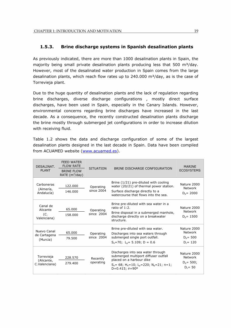
CHAPTER 1: INTRODUCTION AND MOTIVATION 19
1.5.3. Brine discharge systems in Spanish desalination plants
As previously indicated, there are more than 1000 desalination plants in Spain, the
majority being small private desalination plants producing less that 500 m³/day.
However, most of the desalinated water production in Spain comes from the large
desalination plants, which reach flow rates up to 240.000 m³/day, as is the case of
Torrevieja plant.
Due to the huge quantity of desalination plants and the lack of regulation regarding
brine discharges, diverse discharge configurations , mostly direct surface
discharges, have been used in Spain, especially in the Canary Islands. However,
environmental concerns regarding brine discharges have increased in the last
decade. As a consequence, the recently constructed desalination plants discharge
the brine mostly through submerged jet configurations in order to increase dilution
with receiving fluid.
Table 1.2 shows the data and discharge configuration of some of the largest
desalination plants designed in the last decade in Spain. Data have been compiled
from ACUAMED website (www.acuamed.es).
DESALINAT. PLANT
FEED WATER FLOW RATE
BRINE FLOW RATE (m3/day)
SITUATION BRINE DISCHARGE CONFIGURATION MARINE
ECOSYSTEMS
Carboneras (Almería, Andalucía)
122.000
146.000
Operating since 2004
Brine (1/21) pre-diluted with cooling water (20/21) of thermal power station.
Surface discharge directly to a watercourse that flows into the sea.
Nature 2000 Network
Dp= 2000
Canal de Alicante
(C. Valenciana)
65.000
158.000
Operating since 2004
Brine pre-diluted with sea water in a ratio of 1:2.
Brine disposal in a submerged manhole, discharge directly on a breakwater structure.
Nature 2000 Network
Dp= 1500
Nuevo Canal de Cartagena
(Murcia)
65.000
79.500
Operating since 2004
Brine pre-diluted with sea water.
Discharges into sea waters through submerged single port outfall.
So=70; Lp= 5.109; D = 0.6
Nature 2000 Network
Dp= 500
Dc= 120
Torrevieja (Alicante,
C.Valenciana)
228.570
279.400
Recently operating
Discharges into sea water through submerged multiport diffuser outfall placed on a harbour dike
So= 68; HA=10; Lp=220; Np=21; n=1; D=0.415; =90º
Nature 2000 Network
Dp= 500;
Dc= 50
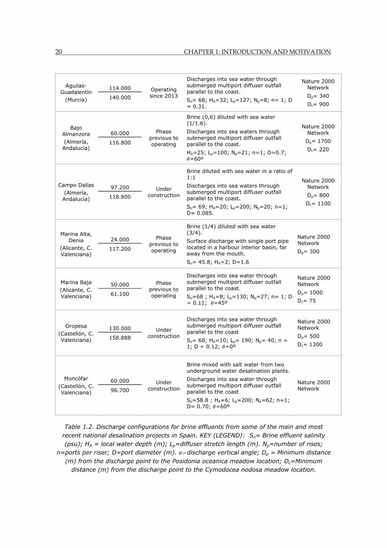
20 CHAPTER 1: INTRODUCTION AND MOTIVATION
Aguilas-Guadalentín
(Murcia)
114.000
140.000
Operating since 2013
Discharges into sea water through submerged multiport diffuser outfall parallel to the coast.
So= 68; HA=32; Lp=127; Np=8; n= 1; D = 0.31.
Nature 2000 Network
Dp= 340
Dc= 900
Bajo Almanzora (Almería, Andalucía)
60.000
116.800
Phase previous to operating
Brine (0,6) diluted with sea water (1/1.6).
Discharges into sea waters through submerged multiport diffuser outfall parallel to the coast.
HA=25; Lp=100; Np=21; n=1; D=0.7; =60º
Nature 2000 Network
Dp= 1700
Dc= 220
Campo Dalías (Almería, Andalucía)
97.200
118.800
Under construction
Brine diluted with sea water in a ratio of 1:1
Discharges into sea waters through submerged multiport diffuser outfall parallel to the coast.
So= 69; HA=20; Lp=200; Np=20; n=1; D= 0.085.
Nature 2000 Network
Dp= 800
Dc= 1100
Marina Alta, Denia
(Alicante, C. Valenciana)
24.000
117.200
Phase previous to operating
Brine (1/4) diluted with sea water (3/4).
Surface discharge with single port pipe located in a harbour interior basin, far away from the mouth.
So= 45.8; HA=2; D=1.6
Nature 2000 Network
Dp= 300
Marina Baja (Alicante, C. Valenciana)
50.000
61.100
Phase previous to operating
Discharges into sea water through submerged multiport diffuser outfall parallel to the coast.
So=68 ; HA=8; Lp=130; Np=27; n= 1; D = 0.11; =45º
Nature 2000 Network
Dp= 1000
Dc= 75
Oropesa (Castellón, C. Valenciana)
130.000
158.888
Under construction
Discharges into sea water through submerged multiport diffuser outfall parallel to the coast
So= 68; HA=10; Lp= 190; Np= 40; n = 1; D = 0.12; =0º
Nature 2000 Network
Dp= 500
Dc= 1300
Moncófar (Castellón, C. Valenciana)
60.000
96.700
Under construction
Brine mixed with salt water from two underground water desalination plants.
Discharges into sea water through submerged multiport diffuser outfall parallel to the coast
So=58.8 ; HA=6; Lp=200; Np=62; n=1; D= 0.70; =60º
Nature 2000 Network
Table 1.2. Discharge configurations for brine effluents from some of the main and most recent national desalination projects in Spain. KEY (LEGEND): So= Brine effluent salinity (psu); HA = local water depth (m); Lp=diffuser stretch length (m). Np=number of rises;
n=ports per riser; D=port diameter (m). discharge vertical angle; Dp = Minimum distance (m) from the discharge point to the Posidonia oceanica meadow location; Dc=Minimum
distance (m) from the discharge point to the Cymodocea nodosa meadow location.
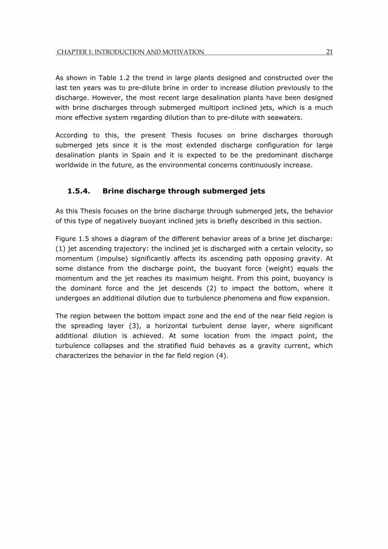
CHAPTER 1: INTRODUCTION AND MOTIVATION 21
As shown in Table 1.2 the trend in large plants designed and constructed over the
last ten years was to pre-dilute brine in order to increase dilution previously to the
discharge. However, the most recent large desalination plants have been designed
with brine discharges through submerged multiport inclined jets, which is a much
more effective system regarding dilution than to pre-dilute with seawaters.
According to this, the present Thesis focuses on brine discharges thorough
submerged jets since it is the most extended discharge configuration for large
desalination plants in Spain and it is expected to be the predominant discharge
worldwide in the future, as the environmental concerns continuously increase.
1.5.4. Brine discharge through submerged jets
As this Thesis focuses on the brine discharge through submerged jets, the behavior
of this type of negatively buoyant inclined jets is briefly described in this section.
Figure 1.5 shows a diagram of the different behavior areas of a brine jet discharge:
(1) jet ascending trajectory: the inclined jet is discharged with a certain velocity, so
momentum (impulse) significantly affects its ascending path opposing gravity. At
some distance from the discharge point, the buoyant force (weight) equals the
momentum and the jet reaches its maximum height. From this point, buoyancy is
the dominant force and the jet descends (2) to impact the bottom, where it
undergoes an additional dilution due to turbulence phenomena and flow expansion.
The region between the bottom impact zone and the end of the near field region is
the spreading layer (3), a horizontal turbulent dense layer, where significant
additional dilution is achieved. At some location from the impact point, the
turbulence collapses and the stratified fluid behaves as a gravity current, which
characterizes the behavior in the far field region (4).
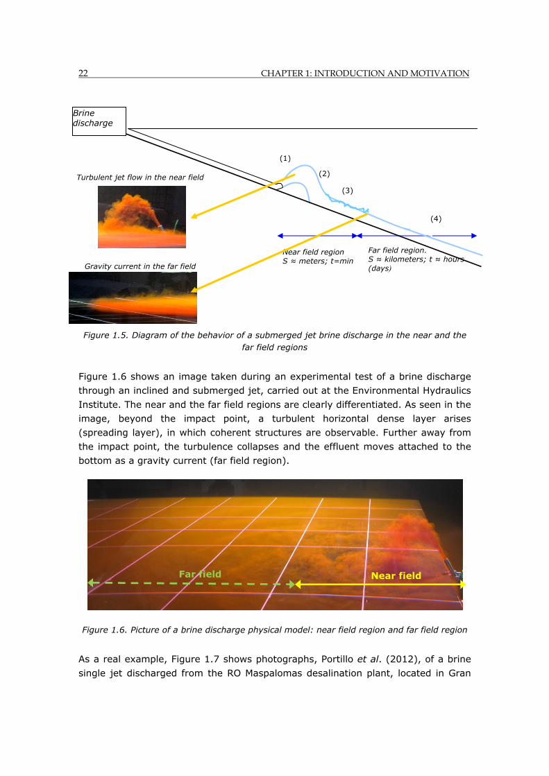
22 CHAPTER 1: INTRODUCTION AND MOTIVATION
Figure 1.5. Diagram of the behavior of a submerged jet brine discharge in the near and the far field regions
Figure 1.6 shows an image taken during an experimental test of a brine discharge
through an inclined and submerged jet, carried out at the Environmental Hydraulics
Institute. The near and the far field regions are clearly differentiated. As seen in the
image, beyond the impact point, a turbulent horizontal dense layer arises
(spreading layer), in which coherent structures are observable. Further away from
the impact point, the turbulence collapses and the effluent moves attached to the
bottom as a gravity current (far field region).
Figure 1.6. Picture of a brine discharge physical model: near field region and far field region
As a real example, Figure 1.7 shows photographs, Portillo et al. (2012), of a brine
single jet discharged from the RO Maspalomas desalination plant, located in Gran
Gravity current in the far field
Turbulent jet flow in the near field
(1)
(2)
(3)
Near field region S ≈ meters; t=min
Far field region. S ≈ kilometers; t ≈ hours (days)
Brine discharge
(4)
Near field Far field

CHAPTER 1: INTRODUCTION AND MOTIVATION 23
Canaria Island (Spain). Brine is coloured with rhodamine in order to study ad hoc
the behavior of the effluent discharged, in the near region (profile view in panel “A”
and plan view in panel “B”) and in the far field region (panel “C”).
Figure 1.7. Pictures from an ad hoc brine jet discharge of coloured brine in Maspalomas beach. Near field region (panels A and B) and far field region (panel C). Source: ITC
1.6. Impacts of brine on the marine environment
The main environmental impacts of desalination projects are associated with the
construction of marine structures, the wastewater disposal and the energy
consumption. The importance of these impacts depends on the type of technology
used in salt separation.
RO plants have a high energy consumption, although it is much lower than in MSF
plants, Afgan et al. (1998). The waste effluent or brine has no chemical or thermal
pollution, but the salt concentration is very high, making it denser than seawater
and thus increasing the risk of negative effects on stenohaline benthic ecosystems.
RO plants do not include combustion processes, resulting in no air pollution. Its
visual impact is less because the plants are usually compact. However, an
additional solid waste is generated by RO, derived from the filters and membranes
cleaning operations, Hoepner. (1990).
A B
C
24 CHAPTER 1: INTRODUCTION AND MOTIVATION
In the last decades, different studies have been carried out to determine the effects
of brine on the marine environment. A summary of the most adverse effects
identified is presented next:
◦ Anoxia at the bottom. In the far field region, brine is a hypersaline plume, which
flows down the seabed, Gacia et al. (2007). The water column appears stratified,
with a pycnocline separating the different layers. The pycnocline hinders the
mixture of layers and reduces the rate of water renewal in the bottom layer,
causing anoxia at the seabed and affecting benthic ecosystems, Hodges (2006).
◦ Turbidity, especially in the brine discharge area, generates a foggy ambient due
to the different light refraction in effluents with a different density, Pérez-Talavera
et al. (2001). Turbidity affects seagrasses by reducing the percentage of light
filtered through the water column that reaches the seabed, thus affecting
photosynthetic benthic organisms, such as seagrasses, Einav et al. (2003). This
impact is more significant in discharges through jets.
◦ Impact on plankton by causing a drop in osmotic pressure (breaking the osmotic
equilibrium between plankton organisms and seawater) and hence causing negative
effects in primary production. Invertebrates have a different sensitivity depending
on their morphology.
◦ Negative effects on equinoderms, for which the exposure to a continuous brine
discharge increases the risk of disappearance of the original communities and their
replacement by opportunist and more resistant species, such as serpulid
polychaetes, etc., Chester (1978). These effects have also been detected, Lloret et
al. (2001) using sea urchin (Paracentrotrus lividus) and mysids (Leptomysis
posidoniae) as bioindicators.
◦ Coral reefs, RPS (2010), are very sensitive to changes in environmental
conditions (chemical pollution, hydrodynamic alterations, temperature, salinity,
etc.), and thus, brine disposal may have significant negative effects.
◦ Impacts on seagrass, mainly due to turbidity and excess of salinity associated to
brine disposal. Seagrasses are aquatic plants, with flowers and fruits, which
colonize seabeds and form huge marine forests in seas and oceans.
The excess of salinity of the brine effluent can negatively affect seagrasses
depending on the sensitivity of the species. Studies on marine angiosperms have
detected a low tolerance to salinity and temperature changes in the conditions of
the receiving environment. In the Mediterranean Sea there are ecologically
CHAPTER 1: INTRODUCTION AND MOTIVATION 25
important angiosperms, Fernández-Torquemada et al. (2005) as is the case of
Posidonia oceanica, Cymodocea nodosa, Zostera noltii, etc.
Posidonia oceanica is an endemic angiosperm of the Mediterranean Sea, designated
as a priority habitat type to be protected in Special Areas of Conservation SACs
“Posidonia beds”, by the EU Directive 92/43/EEC. This habitat is considered a
marine climax community, constituting huge forests that cover the sandy bottoms
at local water depths below 40 meters, where filtered light is sufficient to carry out
photosynthesis. This seagrass performs several important ecological functions:
fixing sand sediment on the seabed; creating a refuge and nourishment zone for
reproduction and growth of diverse species; supporting epiphytes in its leaves;
generating oxygen and organic matter; consuming carbon dioxide and also
protecting the coast against the swell waves, Sánchez-Lizaso et al. (2008).
Posidonia oceanica is adapted to calm seawater and stable physical and chemical
characteristics of the Mediterranean Sea, and it is very sensitive to changes. In
particular, Posidonia is a stenohaline species, as it tolerates only slight variations in
salt concentration. It is also affected negatively by the turbidity and contaminant
substances, Gacia et al. (2007). Due to its ecological importance and fragility, the
Posidonia oceanica is considered one of the main habitats requiring protection in
the Mediterranean Sea.
Cymodocea nodosa is another important seagrass in the Mediterranean, Einav et al.
(2003), Terrados et al. (1992). It grows at lower depths than Posidonia and is more
resistant to energetic hydrodynamics, variations in salinity or pollutant
concentration. It usually covers a type of seabed that is also protected, catalogued
as a SAC, by the EU Directive 92/43/EEC. Other important benthic communities in
the Mediterranean Sea are the Zostera noltii meadows.
Several studies on angiosperms and algae have detected a decrease in growth,
tissue necrosis, leaf loss and an increment of the mortality rate when exposed to
increasing salinities. One of the most important research on the topic was carried
out in Spain with the purpose of establishing critical salinity limits to guarantee the
conservation of Posidonia oceanica meadows. Both laboratory model tests and field
control campaigns on Posidonia meadows exposed to brine disposals over fifteen
day periods were carried out, Sánchez-Lizaso et al. (2008). Based on the results
and conclusions obtained, critical salinity limits were established as quality criteria.
These thresholds (in psu: practical salinity units), together with those established
for other species in the Mediterranean Sea, as shown in Table 1.3.
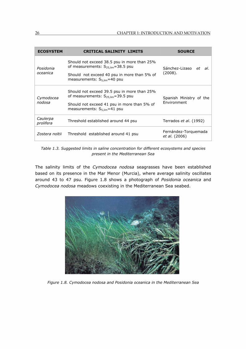
26 CHAPTER 1: INTRODUCTION AND MOTIVATION
ECOSYSTEM CRITICAL SALINITY LIMITS SOURCE
Posidonia oceanica
Should not exceed 38.5 psu in more than 25% of measurements: S25,lim=38.5 psu
Should not exceed 40 psu in more than 5% of measurements: S5,lim=40 psu
Sánchez-Lizaso et al. (2008).
Cymodocea nodosa
Should not exceed 39.5 psu in more than 25% of measurements: S25,lim=39.5 psu
Should not exceed 41 psu in more than 5% of measurements: S5,lim=41 psu
Spanish Ministry of the Environment
Caulerpa prolifera
Threshold established around 44 psu Terrados et al. (1992)
Zostera noltii Threshold established around 41 psu Fernández-Torquemada et al. (2006)
Table 1.3. Suggested limits in saline concentration for different ecosystems and species present in the Mediterranean Sea
The salinity limits of the Cymodocea nodosa seagrasses have been established
based on its presence in the Mar Menor (Murcia), where average salinity oscillates
around 43 to 47 psu. Figure 1.8 shows a photograph of Posidonia oceanica and
Cymodocea nodosa meadows coexisting in the Mediterranean Sea seabed.
Figure 1.8. Cymodocea nodosa and Posidonia oceanica in the Mediterranean Sea

CHAPTER 1: INTRODUCTION AND MOTIVATION 27
1.7. Environmental impact assessment and regulation of brine discharges
Despite the increasing desalination production and the evidence of negative effects
on the marine environment, at the moment there is no Spanish or European
legislation in place regulating brine discharges into seawaters. In particular, brine
properties emission limits or water quality standards to protect the receiving waters
have not been established and neither criteria to design brine discharges, to predict
its behavior or to environmental evaluate its potential impact.
The Water Quality EU Directives do not set critical limits on the discharged brine or
water quality standards on receiving water bodies in order to guarantee the marine
environment protection against brine discharges. Directives related to discharges or
water quality, such as Directive 2006/11/EC on pollution caused by certain
dangerous substances discharged into the aquatic environment of the European
Union does not include the chemical additives usually present in brine or the excess
of salinity. The 91/271/EEC Directive concerning urban wastewater treatment
(modified by the 98/15/EC) neither includes any reference to brine. Furthermore,
Council Directive 76/160/EEC concerning the quality of bathing water or Directive
2006/113/EC on the quality required of shellfish waters establish critical thresholds
of some substances within the water environment, but do not include those relative
to brine.
The Water Framework Directive (Directive 2000/60/EC) includes salinity as a
physical and chemical indicator. However, there are no limits for this parameter. In
Spain, the regulation in force: “Instrucción para el proyecto de conducciones de
vertido desde tierra el mar” (O. M. 13 de Julio de 1993), developed for sewage
discharges, includes some specifications which can be also applied to outfalls of
brine discharges. However, these specifications cover a very small number of the
aspects that must be considered, and they are mainly related to the structure
preservation during the operation phase.
Moreover, the assessment of the Environmental Impact Studies (EIS) of the largest
Spanish desalination plants carried out in this work, have revealed important lacks
of knowledge, criteria and methodologies in many aspects to consider in the brine
discharges. These gaps lead to significant uncertainties in the environmental
evaluation of this type of discharges, increasing the risk of significant impacts on
marine species.
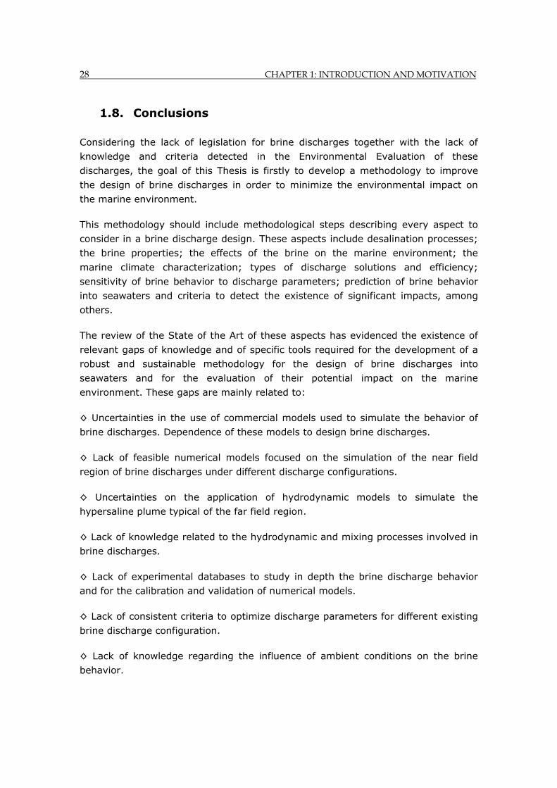
28 CHAPTER 1: INTRODUCTION AND MOTIVATION
1.8. Conclusions
Considering the lack of legislation for brine discharges together with the lack of
knowledge and criteria detected in the Environmental Evaluation of these
discharges, the goal of this Thesis is firstly to develop a methodology to improve
the design of brine discharges in order to minimize the environmental impact on
the marine environment.
This methodology should include methodological steps describing every aspect to
consider in a brine discharge design. These aspects include desalination processes;
the brine properties; the effects of the brine on the marine environment; the
marine climate characterization; types of discharge solutions and efficiency;
sensitivity of brine behavior to discharge parameters; prediction of brine behavior
into seawaters and criteria to detect the existence of significant impacts, among
others.
The review of the State of the Art of these aspects has evidenced the existence of
relevant gaps of knowledge and of specific tools required for the development of a
robust and sustainable methodology for the design of brine discharges into
seawaters and for the evaluation of their potential impact on the marine
environment. These gaps are mainly related to:
◊ Uncertainties in the use of commercial models used to simulate the behavior of
brine discharges. Dependence of these models to design brine discharges.
◊ Lack of feasible numerical models focused on the simulation of the near field
region of brine discharges under different discharge configurations.
◊ Uncertainties on the application of hydrodynamic models to simulate the
hypersaline plume typical of the far field region.
◊ Lack of knowledge related to the hydrodynamic and mixing processes involved in
brine discharges.
◊ Lack of experimental databases to study in depth the brine discharge behavior
and for the calibration and validation of numerical models.
◊ Lack of consistent criteria to optimize discharge parameters for different existing
brine discharge configuration.
◊ Lack of knowledge regarding the influence of ambient conditions on the brine
behavior.

CHAPTER 1: INTRODUCTION AND MOTIVATION 29
◊ Lack of databases and methodologies to characterize and consider climate
variables that significantly affect the brine behavior.
◊ Lack of a methodology to define the statistical scenarios representative of the
desalination plant operational conditions and the marine ambient conditions.
◊ Lack of critical salinity limits for brine-sensitive and with ecological value. These
thresholds have to be defined based on fieldwork and experimental work in the
laboratory.
Faced with these statements, various additional objectives have been set out in the
present Thesis in order to improve some of the gaps detected as described in the
following Chapter.

30 CHAPTER 1: INTRODUCTION AND MOTIVATION
CHAPTER 2. OBJECTIVES AND METHODOLOGY 31
Chapter 2. OBJECTIVES AND METHODOLOGY
Chapter 2 OBJECTIVES AND METHODOLOGY
2.1. Objectives.
According to that explained in Chapter 1, the current situation of desalination in
Spain and the uncertainties in the brine management motivate the main objective
of this Thesis, namely of developing a methodology to improve the design of brine
discharges into seawaters in order to minimize the negative effects on the marine
environment.
As a summary of Chapter 1, Figure 2.1 shows a flowchart with the main aspects
and steps to consider in the design of brine discharges from an environmental point
of view to guarantee the accomplishment of the water quality standards (in
particular, salinity), established to protect the marine sensitive species. For this
environmental assessment, the brine behavior requires to be predicted using
numerical or experimental models and ambient scenarios representative of the real
conditions have to be defined. For the brine behavior predictions, the effluent
characteristics, the marine climate and the discharge configuration have to be
defined.
The present work focuses on brine from seawater reverse osmosis desalination
plants, as the most promising technology of the future. Among the configurations
existing, the present work deals with discharges through submerged jets since it is
the most effective solution to achieve high dilutions and therefore the most used in
large desalination plants and sensitive marine areas.
In the flowchart displayed below, the main aspects to consider in the design of a
brine discharge are included, highlighting with red circles, the main knowledge gaps
identified in Section 1.8.
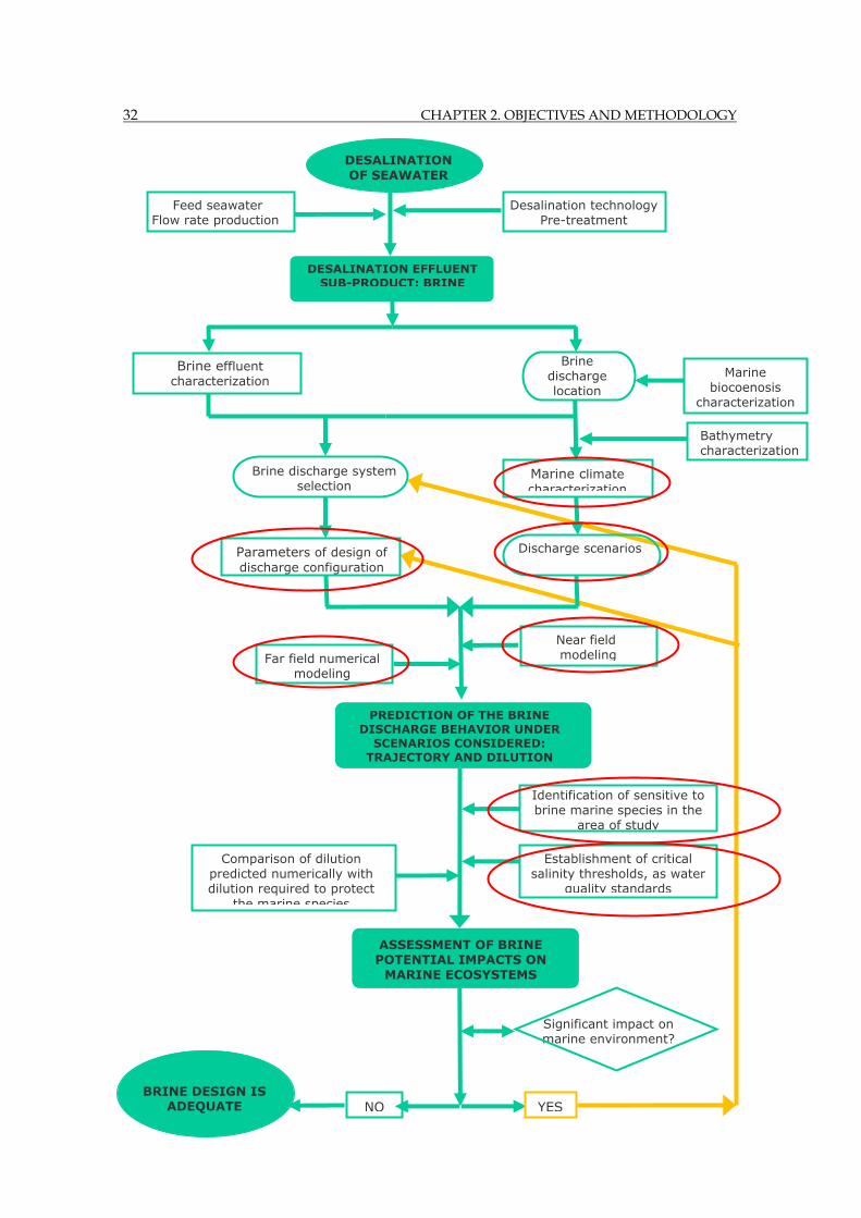
32 CHAPTER 2. OBJECTIVES AND METHODOLOGY
PREDICTION OF THE BRINE DISCHARGE BEHAVIOR UNDER
SCENARIOS CONSIDERED: TRAJECTORY AND DILUTION
NO
Significant impact on marine environment?
DESALINATION OF SEAWATER
DESALINATION EFFLUENT SUB-PRODUCT: BRINE
Desalination technology Pre-treatment
Brine discharge system selection
Brine discharge location
Near field modeling
Marine climate characterization
Parameters of design of discharge configuration
ASSESSMENT OF BRINE POTENTIAL IMPACTS ON
MARINE ECOSYSTEMS
Identification of sensitive to brine marine species in the
area of study
Establishment of critical salinity thresholds, as water
quality standards
Feed seawater Flow rate production
Brine effluent characterization
Discharge scenarios
Marine biocoenosis
characterization
Far field numerical modeling
Bathymetry characterization
Comparison of dilution predicted numerically with dilution required to protect
the marine species
YES
BRINE DESIGN IS
ADEQUATE

CHAPTER 2. OBJECTIVES AND METHODOLOGY 33
This Thesis is devoted to four of these gaps, which will be explored in depth. With
the aim of developing a methodology to design brine discharges, these gaps lead to
the following four additional partial objectives that need to be addressed in the
present work:
Regarding experimental modeling:
● To analyze experimentally the behavior of brine discharges, implementing, to our
knowledge, for the first time in Spain, non-intrusive laser anemometry techniques to study this type of flow. For this task, a set of experimental tests has been carried out in the Environmental Hydraulics Institute, generating an experimental database with a high quality and a large spatial and time resolution, adequate to deepen in the flow processes and to calibrate and validate numerical models. This task is described in Chapter 5.
Regarding numerical modeling:
● To analyze the existing and most used commercial models to simulate the near
field region of brine discharges and to validate them with experimental data, assessing their reliability and feasibility degree. The final goal is to provide useful information to users and to provide recommendations for an adequate application of these models. This task is presented in Chapters 3 and 4.
● To go in depth in the study and characterization of the hydrodynamic and mixing
processes governing the behavior of negatively buoyant effluents, such as brine.
Moreover, to validate the simplified hypothesis commonly assumed by numerical
models simulating this type of flow. This task has been carried out by analyzing the
experimental data obtained from the test carried out in this work and is presented
in Chapters 6, 7 and 8.
● Face to commercial model limitations, to develop new simulation tools for brine
discharges, calibrating them with experimental data to get a better fit to the real
behavior of this type of flow. “brIHne” have arisen with this objective, as explained
in Chapter 9.
The conclusions, recommendations and tools developed by meeting the said four
objectives have been included as part of the methodological guidelines to design
brine discharges, which are described in Chapter 10, with improve of scientific
foundations.
34 CHAPTER 2. OBJECTIVES AND METHODOLOGY
2.2. Methodology.
The starting point of the present work has been the direct involvement in the
Environmental Assessment of the desalination plants of the Spanish National
Hydrological Plan (NHP, 2005) and the review of a huge quantity of Environmental
Impact Studies of older desalination plants, State Environmental Impact
Statements and local Discharge Authorizations.
At this first stage, carried out working for the Spanish Ministry of the Environment,
the main aspects to be considered in the Environmental Assessment of a brine
discharge have been defined. Furthermore, the main gaps, uncertainties, errors and
knowledge needs related to the brine discharge behavior and its potential impact on
the environment have been identified.
An exhaustive review of the State of the Art of each of these main aspects has been
carried out next, including very diverse topics, such as desalination processes,
biological aspects and experimental and numerical modeling, among others. This
review allows solving some of the uncertainties identified in the Spanish
Environmental Impact Studies of desalination plants and at the same time detecting
the lack of scientific knowledge or tools necessary to develop a rigorous
methodology for the design of brine discharges and assess their impacts on the
environment. This review of the State of the Art and identification of the topics
requiring a further investigation was the base of the present Thesis.
Next, the sequence of steps followed in developing this Thesis is presented in the
list below:
1. Setting up the goals of the Thesis, according to the gaps and needs
detected in the previous study: to develop a methodology for the
improvement of the design of brine discharges, and to explore in depth
some of the topics for which the lack of scientific knowledge makes further
research necessary.
2. To carry out the analysis and validation of the most used commercial
models to simulate brine discharges, determining the degree of reliability
and setting up recommendations.
3. To develop the methodology for characterizing brine discharges through
anemometry laser experimental techniques. To carry out experimental tests

CHAPTER 2. OBJECTIVES AND METHODOLOGY 35
in the IH Cantabria laboratory, obtaining an experimental database
regarding brine discharges, with high quality and time and spatial
resolution.
4. Characterization of the brine behavior and study of the hydrodynamic
and mixing processes of the brine flow through the analysis of the
experimental data. Assessment of the reliability degree regarding the
simplifying hypothesis assumed by the mathematical approaches of this
type of flow.
5. Development of new modeling tools (“brIHne” tools) focused on brine
discharges, based on the most adequate mathematical approaches, and
calibrated with the experimental data obtained from the present work.
6. Defining the methodological steps in the design of brine discharges to
minimize the potential negative impact on the marine environment.
Integration of the conclusions, recommendations and tools developed in the
present work.
7. Application of the methodology to a case study.
8. Application for end users.

36 CHAPTER 2. OBJECTIVES AND METHODOLOGY

CHAPTER 3. ANALYSIS OF COMMERCIAL MODELS 37
Chapter 3. ANALYSIS OF COMMERCIAL MODELS FOR BRINE DISCHARGES
Chapter 3 ANALYSIS OF COMMERCIAL MODELS FOR BRINE DISCHARGES
Summary
Regarding brine discharges, CORMIX, VISUAL PLUMES and VISJET software are the
most used by designers to predict the behavior of this type of negatively buoyant
effluents. However, uncertainties detected in old and recent Environmental Impact
Studies and Environmental Authorizations makes it necessary to carry out an
exhaustive analysis of these commercial models when simulating brine discharges.
With this goal, this chapter presents an exhaustive analysis of these commercial
models, including the theoretical base, major assumptions, capabilities, limitations,
sensitivity analysis and an assessment of the reliability degree of these models in
the simulation of brine discharges. Based on this analysis, conclusions and
recommendations have arisen.
The analysis presented in this chapter is completed in Chapter 4, carrying out a
validation of the results obtained from these commercial tools against experimental
data found in the literature, focusing on discharges through jets into stagnant and
dynamic environments.
These two chapters represent a global research of the degree of reliability of
existing commercial tools and provide useful information for the technical and
scientific communities. The conclusions outlined in this work intend to improve the
quality of environmental impact assessments of desalination projects, reducing the
uncertainty associated with the use of commercial models.
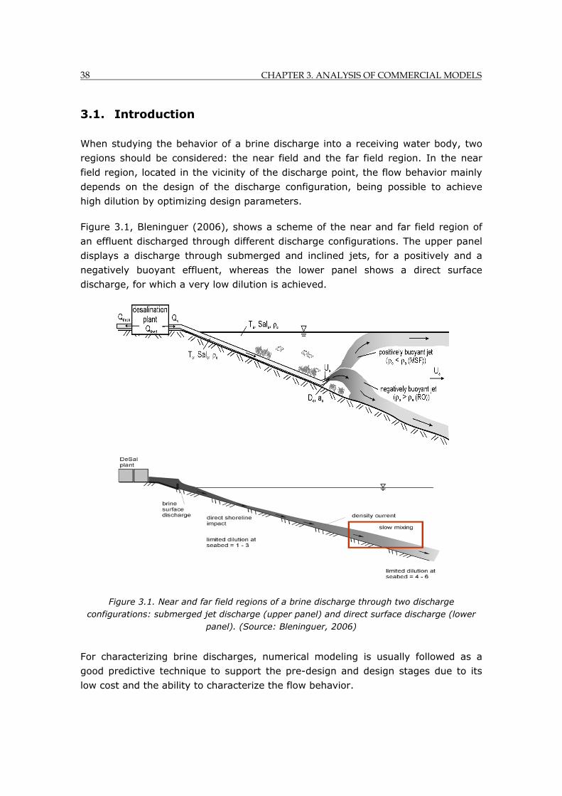
38 CHAPTER 3. ANALYSIS OF COMMERCIAL MODELS
3.1. Introduction
When studying the behavior of a brine discharge into a receiving water body, two
regions should be considered: the near field and the far field region. In the near
field region, located in the vicinity of the discharge point, the flow behavior mainly
depends on the design of the discharge configuration, being possible to achieve
high dilution by optimizing design parameters.
Figure 3.1, Bleninguer (2006), shows a scheme of the near and far field region of
an effluent discharged through different discharge configurations. The upper panel
displays a discharge through submerged and inclined jets, for a positively and a
negatively buoyant effluent, whereas the lower panel shows a direct surface
discharge, for which a very low dilution is achieved.
Figure 3.1. Near and far field regions of a brine discharge through two discharge configurations: submerged jet discharge (upper panel) and direct surface discharge (lower
panel). (Source: Bleninguer, 2006)
For characterizing brine discharges, numerical modeling is usually followed as a
good predictive technique to support the pre-design and design stages due to its
low cost and the ability to characterize the flow behavior.
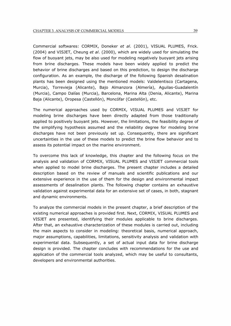
CHAPTER 3. ANALYSIS OF COMMERCIAL MODELS 39
Commercial softwares: CORMIX, Doneker et al. (2001), VISUAL PLUMES, Frick.
(2004) and VISJET, Cheung et al. (2000), which are widely used for simulating the
flow of buoyant jets, may be also used for modeling negatively buoyant jets arising
from brine discharges. These models have been widely applied to predict the
behavior of brine discharges and based on this prediction, to design the discharge
configuration. As an example, the discharge of the following Spanish desalination
plants has been designed using the mentioned models: Valdelentisco (Cartagena,
Murcia), Torrevieja (Alicante), Bajo Almanzora (Almería), Aguilas-Guadalentín
(Murcia), Campo Dalías (Murcia), Barcelona, Marina Alta (Denia, Alicante), Marina
Baja (Alicante), Oropesa (Castellón), Moncófar (Castellón), etc.
The numerical approaches used by CORMIX, VISUAL PLUMES and VISJET for
modeling brine discharges have been directly adapted from those traditionally
applied to positively buoyant jets. However, the limitations, the feasibility degree of
the simplifying hypothesis assumed and the reliability degree for modeling brine
discharges have not been previously set up. Consequently, there are significant
uncertainties in the use of these models to predict the brine flow behavior and to
assess its potential impact on the marine environment.
To overcome this lack of knowledge, this chapter and the following focus on the
analysis and validation of CORMIX, VISUAL PLUMES and VISJET commercial tools
when applied to model brine discharges. The present chapter includes a detailed
description based on the review of manuals and scientific publications and our
extensive experience in the use of them for the design and environmental impact
assessments of desalination plants. The following chapter contains an exhaustive
validation against experimental data for an extensive set of cases, in both, stagnant
and dynamic environments.
To analyze the commercial models in the present chapter, a brief description of the
existing numerical approaches is provided first. Next, CORMIX, VISUAL PLUMES and
VISJET are presented, identifying their modules applicable to brine discharges.
After that, an exhaustive characterization of these modules is carried out, including
the main aspects to consider in modeling: theoretical basis, numerical approach,
major assumptions, capabilities, limitations, sensitivity analysis and validation with
experimental data. Subsequently, a set of actual input data for brine discharge
design is provided. The chapter concludes with recommendations for the use and
application of the commercial tools analyzed, which may be useful to consultants,
developers and environmental authorities.

40 CHAPTER 3. ANALYSIS OF COMMERCIAL MODELS
3.2. Modelling as a predictive tool
Water quality modeling applied to brine discharges solves the hydrodynamic and
transport equations adapted to a negatively buoyant effluent, which can be set up
using a Lagrangian or Eulerian approach.
In most models, the following simplifying assumptions are considered:
incompressible flow, Reynolds decomposition (mean and turbulent components);
Boussinesq approximation (density differences are negligible with the exception of
the terms of the buoyancy force); molecular diffusion is neglected and the turbulent
diffusion closure model is generally based on Boussinesq eddy viscosity theory.
Closure models, such as entrainment formulas, and other experimental parameters
need to be calibrated with experimental data obtained by physical models.
To solve the governing equations, three different approaches are applied, namely
by using dimensional analysis, by integration of ordinary differential equations, and
numerically, with less assumptions, thanks to CFD models. Below, these
approaches are briefly described.
3.2.1. Models based on the dimensional analysis of the relevant processes
Dimensional analysis is the simplest approach and is used to formulate reasonable
hypotheses about complex physical situations that can be tested experimentally. In
dimensional analysis, variables with greater influence on the processes are
considered, with the values of those with less influence held constant, reducing the
number of independent variables under consideration. Selected independent
variables are related through "flux" magnitudes, which represent the major forces
controlling the effluent behavior.
The main fluxes in the discharge process are, Pincince et al. (1973), Fisher et al.
(1979):
▪ Kinematic mass flux ( ): represents the effluent flow discharged into the
receiving environment.
4 4.1
▪ Kinematic momentum flux ( ): represents the energy transported during the
discharge of the effluent.
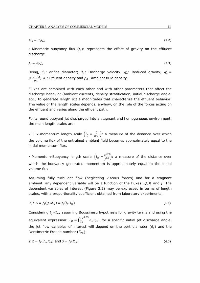
CHAPTER 3. ANALYSIS OF COMMERCIAL MODELS 41
4.2
▪ Kinematic buoyancy flux ( ): represents the effect of gravity on the effluent
discharge.
4.3
Being, : orifice diameter; : Discharge velocity; : Reduced gravity;
; : Effluent density and : Ambient fluid density.
Fluxes are combined with each other and with other parameters that affect the
discharge behavior (ambient currents, density stratification, initial discharge angle,
etc.) to generate length scale magnitudes that characterize the effluent behavior.
The value of the length scales depends, anyhow, on the role of the forces acting on
the effluent and varies along the effluent path.
For a round buoyant jet discharged into a stagnant and homogeneous environment,
the main length scales are:
▪ Flux-momentum length scale / : a measure of the distance over which
the volume flux of the entrained ambient fluid becomes approximately equal to the
initial momentum flux.
▪ Momentum-Buoyancy length scale 3/4
1/2 : a measure of the distance over
which the buoyancy generated momentum is approximately equal to the initial
volume flux.
Assuming fully turbulent flow (neglecting viscous forces) and for a stagnant
ambient, any dependent variable will be a function of the fluxes: , and . The
dependent variables of interest (Figure 3.2) may be expressed in terms of length
scales, with a proportionality coefficient obtained from laboratory experiments.
, , , , , 4.4
Considering , assuming Boussinesq hypothesis for gravity terms and using the
equivalent expression: .
, for a specific initial jet discharge angle,
the jet flow variables of interest will depend on the port diameter ( ) and the
Densimetric Froude number ( ):
, , and 4.5
42 CHAPTER 3. ANALYSIS OF COMMERCIAL MODELS
Where:
: Vertical location. : Horizontal location.
: Dilution rate.
: Densimetric Froude number ( ), being : Jet radius of the round jet.
Formulas based on dimensional analysis have been calibrated by different authors,
thanks to experimental data acquired with conventional or optical measurement
techniques, Roberts et al. (1997), Kikkert et al. (2007), Shao et al. (2010), etc.
These formulas, based on experimental investigation, have been used to validate
the commercial models in the following chapter.
3.2.2. Models based on the integration of differential equations
Integral models are usually applied to simulate the flow of jets or gravity currents.
Governing equations of the flow are in this case integrated over the flow cross
section, transforming them into simple ordinary differential equations, which are
easily solved by numerical methods. Integration of the equations requires assuming
an unlimited receiving water body and consequently boundary effects cannot be
modeled. In the case of jet modeling, even if these models provide detailed
descriptions of the jet behavior, results are only valid along the effluent trajectory
prior to the impact of the jet on the bottom, and if and only if the effluent does not
previously reach the surface or impact with obstacles or lateral boundaries. Hence,
they are limited to the near field region.
Since the results of the integrated equations refer to magnitudes in the jet axis,
calculations of these values in cross-sections require assuming a distribution
function, generally Gaussian or Top-Hat, and experimentally assessing the basic
parameters. Effluent diffusion is controlled in these models by simple “entrainment”
formulas, based mainly on the eddy viscosity concept, with coefficients obtained
experimentally.
Integral models for hyperdense jets have also been presented in several studies,
such as Kikkert et al. (2007) and Cipollina et al. (2009). Entrainment formulas used
to characterize mixing in brine jet discharges in integral models, are analyzed in
Kaminski et al. (2005) and Papanicolau et al. (2008).
CHAPTER 3. ANALYSIS OF COMMERCIAL MODELS 43
3.2.3. Computational Fluid Dynamics (CFDs) models
CFDs are the most rigorous models as they assume fewer simplifying hypotheses.
Due to the high Reynolds number of the studied jets and the high computational
cost, DNS (Direct Numerical Simulation) is not affordable nowadays. However,
hydrodynamics and transport equations can be solved using complex turbulence
closure models of either time (Reynolds equations), or spatially averaged Large
Eddy Simulation (LES). Although very refined information can be extracted from the
simulations, these models are still very time-consuming compared to the integral
model approach.
There are few examples in the literature of CFD commercial models applied to brine
discharge simulations. Plum (2008) applies the CFD FLUENT software to a
submerged single port jet, comparing different turbulence models and validating
them with experimental data in a stagnant and homogeneous environment. Oliver
et al. (2008) studies the influence of the turbulence closure model used for a single
port jet discharge in a stagnant ambient.
At present, these models are not completely developed for brine discharge
modeling and calibration and validation of the turbulence and transport models is
needed for real applications.
3.3. Critical assessment of CORMIX, VISUAL PLUMES and VISJET softwares for brine discharge modelling
3.3.1. Software general description
As previously mentioned, CORMIX, VISUAL PLUMES and VISJET are the most widely
used commercial models to simulate brine discharges. They include different
models for simulating flows with neutral, positive and negative buoyancy,
considering the brine effluent properties, the discharge configuration and the
ambient conditions.
CORMIX (Cornell Mixing Zone Expert System) software, Doneker et al. (2001) was
developed in the 1980s at Cornell University (USA) as a project subsidized by the
Environmental Protection Agency (EPA). Supported by the EPA, it has become one
of the most popular programs for discharge modeling.
It includes three subsystems CORMIX1, 2 and 3, based on dimensional analysis of
the processes, which predict the flow behavior in the near and far field regions.
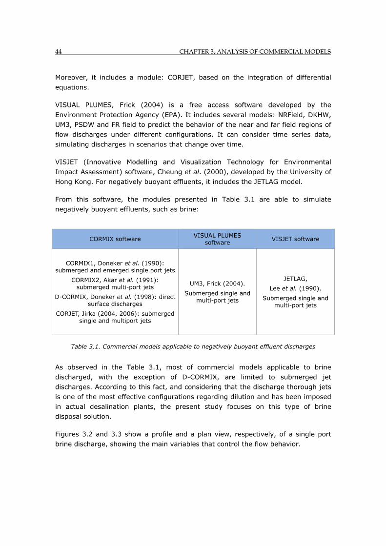
44 CHAPTER 3. ANALYSIS OF COMMERCIAL MODELS
Moreover, it includes a module: CORJET, based on the integration of differential
equations.
VISUAL PLUMES, Frick (2004) is a free access software developed by the
Environment Protection Agency (EPA). It includes several models: NRField, DKHW,
UM3, PSDW and FR field to predict the behavior of the near and far field regions of
flow discharges under different configurations. It can consider time series data,
simulating discharges in scenarios that change over time.
VISJET (Innovative Modelling and Visualization Technology for Environmental
Impact Assessment) software, Cheung et al. (2000), developed by the University of
Hong Kong. For negatively buoyant effluents, it includes the JETLAG model.
From this software, the modules presented in Table 3.1 are able to simulate
negatively buoyant effluents, such as brine:
Table 3.1. Commercial models applicable to negatively buoyant effluent discharges
As observed in the Table 3.1, most of commercial models applicable to brine
discharged, with the exception of D-CORMIX, are limited to submerged jet
discharges. According to this fact, and considering that the discharge thorough jets
is one of the most effective configurations regarding dilution and has been imposed
in actual desalination plants, the present study focuses on this type of brine
disposal solution.
Figures 3.2 and 3.3 show a profile and a plan view, respectively, of a single port
brine discharge, showing the main variables that control the flow behavior.
CORMIX software VISUAL PLUMES
software VISJET software
CORMIX1, Doneker et al. (1990): submerged and emerged single port jets
CORMIX2, Akar et al. (1991): submerged multi-port jets
D-CORMIX, Doneker et al. (1998): direct surface discharges
CORJET, Jirka (2004, 2006): submerged single and multiport jets
UM3, Frick (2004).
Submerged single and multi-port jets
JETLAG,
Lee et al. (1990).
Submerged single and multi-port jets
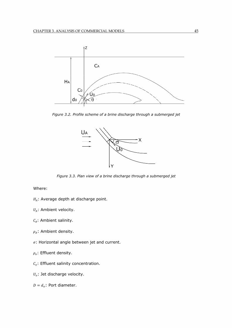
CHAPTER 3. ANALYSIS OF COMMERCIAL MODELS 45
Figure 3.2. Profile scheme of a brine discharge through a submerged jet
Figure 3.3. Plan view of a brine discharge through a submerged jet
Where:
: Average depth at discharge point.
: Ambient velocity.
: Ambient salinity.
: Ambient density.
: Horizontal angle between jet and current.
: Effluent density.
: Effluent salinity concentration.
: Jet discharge velocity.
: Port diameter.

46 CHAPTER 3. ANALYSIS OF COMMERCIAL MODELS
: Port height.
: Jet discharge angle (vertical angle with respect to the bottom).
As a summary of the analysis carried out for each of the commercial models
applicable brine discharged simulations, a set of tables is presented in the next
sections, including the following information:
Application: Type of effluents and discharge configurations simulated.
Modeling approach: Method used for solving governing equations.
Main assumptions: Simplifying hypotheses considered.
Capabilities: Potentials/possibilities/options.
Limitations: Restrictions in modeling.
Sensitivity analysis: conclusions from the sensitivity analysis carried out, varying
the value of the most relevant input data over an actual range of values.
Validation by software authors: Validation studies carried out and published by
the model authors.
Recommendations: Suggestions to users for the most rigorous application and use
of the models.
This information has been gathered from a combination of the material provided
with the software, a literature search and an extensive use of these models in
simulating brine discharges from Spanish desalination plants and from actual cases.
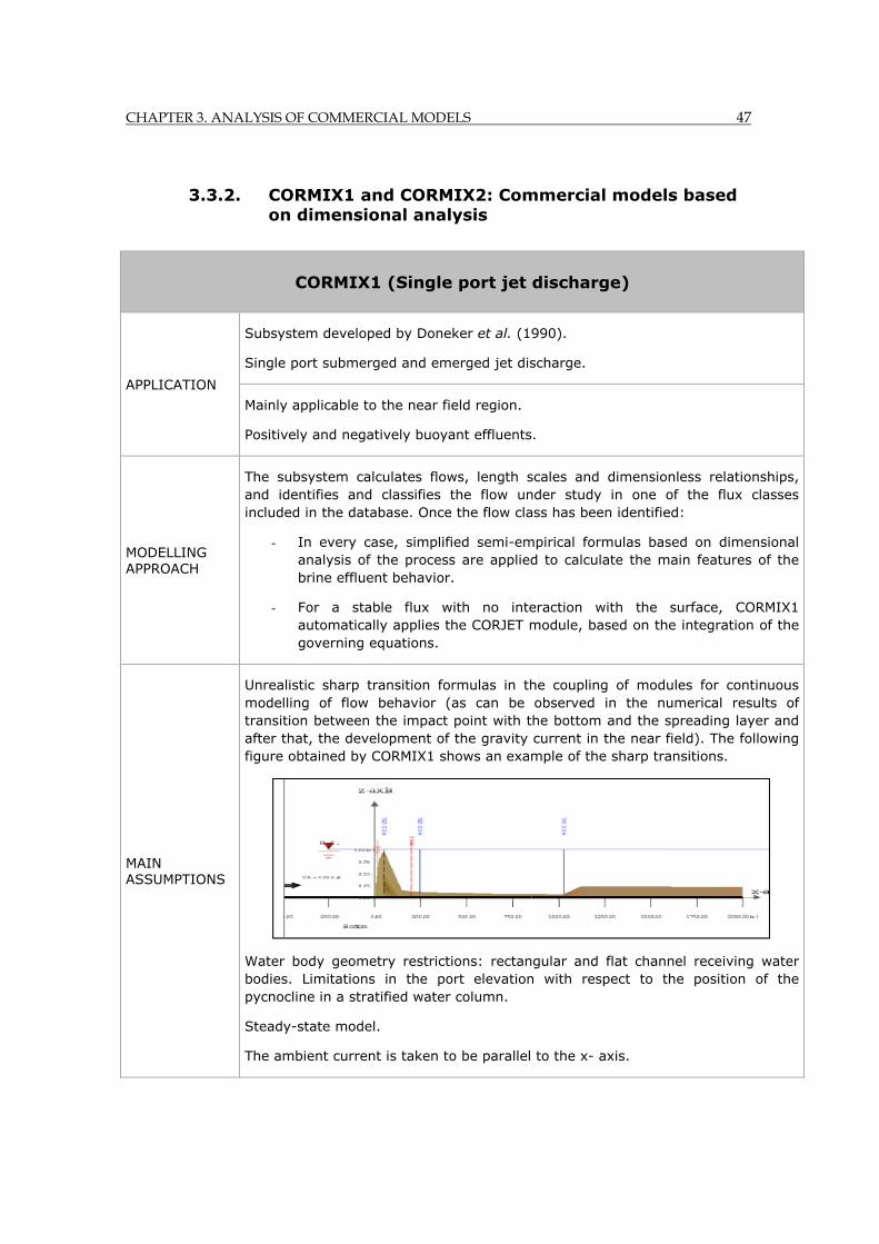
CHAPTER 3. ANALYSIS OF COMMERCIAL MODELS 47
3.3.2. CORMIX1 and CORMIX2: Commercial models based on dimensional analysis
CORMIX1 (Single port jet discharge)
APPLICATION
Subsystem developed by Doneker et al. (1990).
Single port submerged and emerged jet discharge.
Mainly applicable to the near field region.
Positively and negatively buoyant effluents.
MODELLING APPROACH
The subsystem calculates flows, length scales and dimensionless relationships, and identifies and classifies the flow under study in one of the flux classes included in the database. Once the flow class has been identified:
- In every case, simplified semi-empirical formulas based on dimensional analysis of the process are applied to calculate the main features of the brine effluent behavior.
- For a stable flux with no interaction with the surface, CORMIX1 automatically applies the CORJET module, based on the integration of the governing equations.
MAIN ASSUMPTIONS
Unrealistic sharp transition formulas in the coupling of modules for continuous modelling of flow behavior (as can be observed in the numerical results of transition between the impact point with the bottom and the spreading layer and after that, the development of the gravity current in the near field). The following figure obtained by CORMIX1 shows an example of the sharp transitions.
Water body geometry restrictions: rectangular and flat channel receiving water bodies. Limitations in the port elevation with respect to the position of the pycnocline in a stratified water column.
Steady-state model.
The ambient current is taken to be parallel to the x- axis.

48 CHAPTER 3. ANALYSIS OF COMMERCIAL MODELS
CAPABILITIES
The subsystem yields a rough approximation of the spreading layer and the far field region by coupling modules.
The brine properties, the discharge configuration design and the ambient conditions (currents and salinity/temperature stratification) are considered.
Multiple types of flow classification.
Unlimited and confined environments can theoretically be modelled.
LIMITATIONS
Some of the calculations are based on formulas obtained with a control volume approach not properly described in the manuals, where the theoretical basis or experimental evidence of these formulas cannot be found within this work search.
Time series are not considered. Each run corresponds to a single discharge scenario.
Although the model makes an approximation of the spreading layer and far field region, validation data are not presented by the authors for hyperdense effluents.
Although a confined environment can be theoretically modelled, if the flow interacts with the surface, significant simplifications are assumed (i.e. homogenization of effluent within the water column), leading in some cases to significant errors.
When the CORJET module is not applied, CORMIX results are limited to some specific points and they do not calculate the evolution of the flux.
The ambient current is constant within the water column, which cannot be discretized into layers.
Density stratification in the water column is limited to only three types of density stratification profiles.
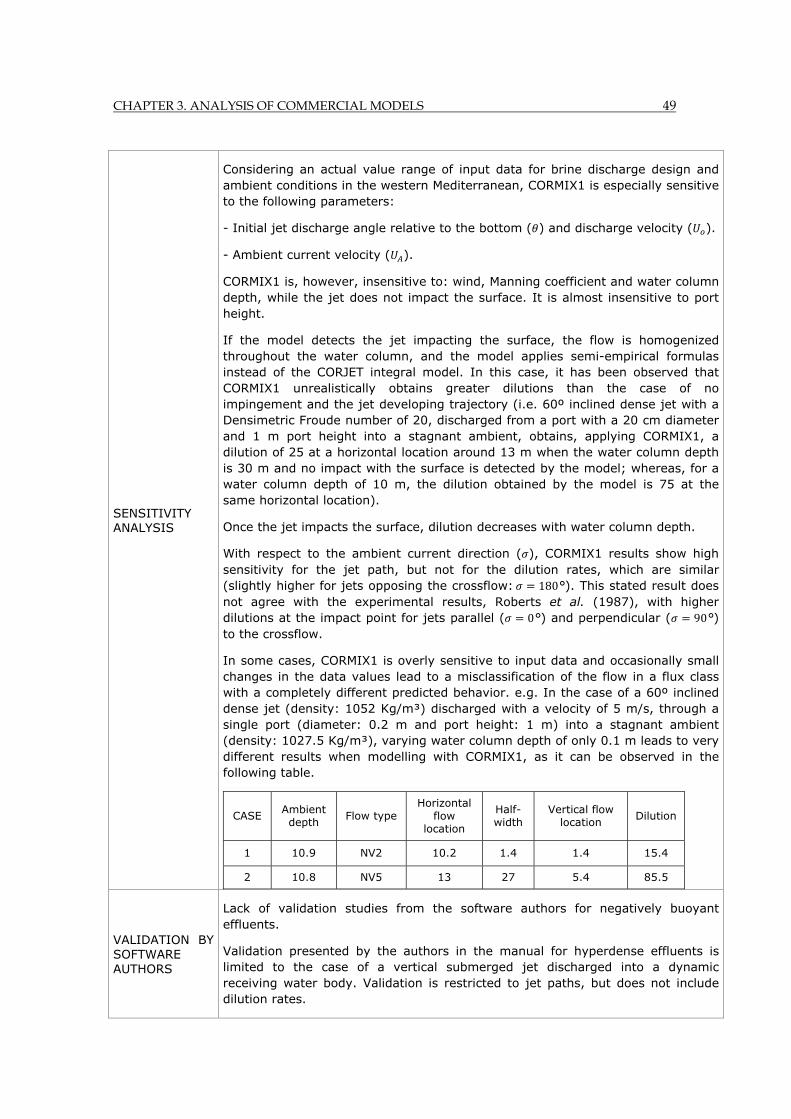
CHAPTER 3. ANALYSIS OF COMMERCIAL MODELS 49
SENSITIVITY ANALYSIS
Considering an actual value range of input data for brine discharge design and ambient conditions in the western Mediterranean, CORMIX1 is especially sensitive to the following parameters:
- Initial jet discharge angle relative to the bottom ( ) and discharge velocity ( ).
- Ambient current velocity ( ).
CORMIX1 is, however, insensitive to: wind, Manning coefficient and water column depth, while the jet does not impact the surface. It is almost insensitive to port height.
If the model detects the jet impacting the surface, the flow is homogenized throughout the water column, and the model applies semi-empirical formulas instead of the CORJET integral model. In this case, it has been observed that CORMIX1 unrealistically obtains greater dilutions than the case of no impingement and the jet developing trajectory (i.e. 60º inclined dense jet with a Densimetric Froude number of 20, discharged from a port with a 20 cm diameter and 1 m port height into a stagnant ambient, obtains, applying CORMIX1, a dilution of 25 at a horizontal location around 13 m when the water column depth is 30 m and no impact with the surface is detected by the model; whereas, for a water column depth of 10 m, the dilution obtained by the model is 75 at the same horizontal location).
Once the jet impacts the surface, dilution decreases with water column depth.
With respect to the ambient current direction ( ), CORMIX1 results show high sensitivity for the jet path, but not for the dilution rates, which are similar (slightly higher for jets opposing the crossflow: 180°). This stated result does not agree with the experimental results, Roberts et al. (1987), with higher dilutions at the impact point for jets parallel ( 0°) and perpendicular ( 90°) to the crossflow.
In some cases, CORMIX1 is overly sensitive to input data and occasionally small changes in the data values lead to a misclassification of the flow in a flux class with a completely different predicted behavior. e.g. In the case of a 60º inclined dense jet (density: 1052 Kg/m³) discharged with a velocity of 5 m/s, through a single port (diameter: 0.2 m and port height: 1 m) into a stagnant ambient (density: 1027.5 Kg/m³), varying water column depth of only 0.1 m leads to very different results when modelling with CORMIX1, as it can be observed in the following table.
CASE Ambient depth
Flow type Horizontal
flow location
Half-width
Vertical flow location
Dilution
1 10.9 NV2 10.2 1.4 1.4 15.4
2 10.8 NV5 13 27 5.4 85.5
VALIDATION BY SOFTWARE AUTHORS
Lack of validation studies from the software authors for negatively buoyant effluents.
Validation presented by the authors in the manual for hyperdense effluents is limited to the case of a vertical submerged jet discharged into a dynamic receiving water body. Validation is restricted to jet paths, but does not include dilution rates.
50 CHAPTER 3. ANALYSIS OF COMMERCIAL MODELS
Table 3.2. Main CORMIX1 features related to brine discharge modeling
MODEL RESULTS RELIABILITY
Reliability depends on the model's ability to reproduce the experimental results used for calibration.
In many cases the type class into which the subsystem classifies the flow does not match those observed experimentally. It has been detected that, in some cases, CORMIX1 predicts the jet impacting the surface, while experiments do not show it. e.g. In the case of a 30º inclined jet, with a Densimetric Froude number of 40, discharged, from a port with a 20 cm diameter and 1 m port height, into a 15 m water column into a stagnant ambient, CORMIX1 considers an unstable flow classified as NH5, homogenized into the entire water column, whereas experimental results and also CORJET, VISJET and JETLAG models model a jet with a maximum rise height around 7 - 9 m.
RECOMMENDATION
When the jets do not impact the surface, it is recommended to directly apply the CORJET module, or both, the CORMIX1 and the CORJET module, comparing the results.
Because the model is in some cases very sensitive to changes in input data, it is recommended to run a set of cases using a range of actual design values.
Since jet behavior simulated by CORMIX1 is very sensitive to ambient current velocity, but almost insensitive to ambient current direction (contradicting experimental results), it is recommended to be cautious about the reliability of the results.
Considering the severe simplifications imposed and the lack of validation data, it is recommended to avoid the use of the CORMIX1 subsystem for far field modelling and for modelling jets impacting the surface.

CHAPTER 3. ANALYSIS OF COMMERCIAL MODELS 51
CAPABILITIES
Same as CORMIX1 and the following:
- A large variety of diffuser multi-port configurations: “single port per riser: unidirectional or alternating”; “two nozzles per riser: less than 60º or about 180º (opposing)”, and “several nozzles per riser” (net momentum flux zero or not zero”) can be chosen by the user.
- Merging between jets and its influence on the trajectory and dilution are simulated.
LIMITATIONS
Same as CORMIX1 and the following:
- Regarding the nozzles in the diffuser: the ports must be of the same diameter, initial discharge angle, port height, velocity, etc., and with the same number of ports per riser, which must be equally spaced.
- Important assumptions are made in diffuser configuration designs, resulting in only two types: 1) a unidirectional diffuser with inclined jets
CORMIX2 (multi-port jet discharge)
APPLICATION
Subsystem developed by Akar et al. (1991).
Multi-port submerged jet discharge.
Mainly applicable to the near field region, but may provide a rough approximation of the spreading layer and the far field region by coupling modules.
Positively and negatively buoyant effluents.
MODELLING APPROACH
The same as CORMIX1 modelling approach
MAIN ASSUMPTIONS
Same as CORMIX1 and the following:
If CORMIX2 does not detect merging between jets, the same length scales and semi-empirical formulas as for CORMIX1 are applied.
If merging between contiguous jets is detected, different assumptions are considered:
- For simple merging processes (the case of unidirectional diffusers), the hypothesis of an equivalent slot diffuser is applied, in which the discharge from the diffuser of equally spaced ports is assumed to be the same as a line slot discharge with the same length conserving the flow fluxes.
- For complex merging processes (in the case of “staged” or “alternating” diffusers) experimental merging formulas are applied.
- For the different types of diffuser configuration, CORMIX2 applies simplifying hypotheses as shown in the “limitations” section.
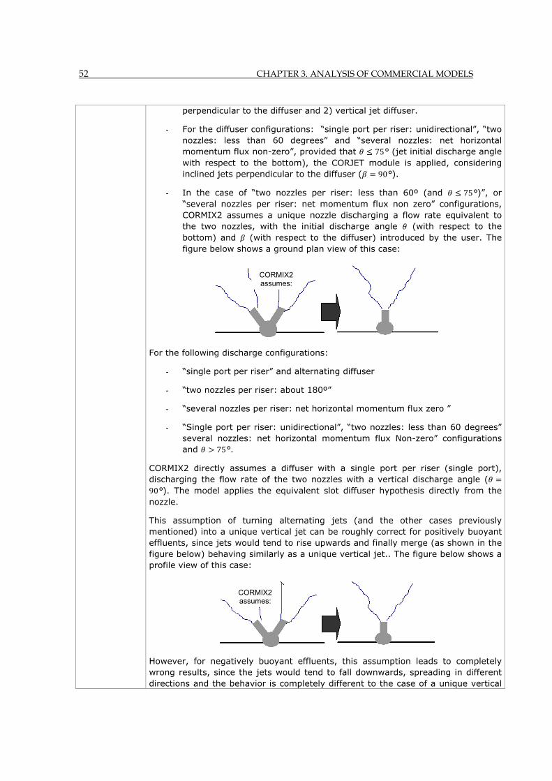
52 CHAPTER 3. ANALYSIS OF COMMERCIAL MODELS
perpendicular to the diffuser and 2) vertical jet diffuser.
- For the diffuser configurations: “single port per riser: unidirectional”, “two nozzles: less than 60 degrees” and “several nozzles: net horizontal momentum flux non-zero”, provided that 75° (jet initial discharge angle with respect to the bottom), the CORJET module is applied, considering inclined jets perpendicular to the diffuser ( 90°).
- In the case of “two nozzles per riser: less than 60º (and 75°)”, or “several nozzles per riser: net momentum flux non zero” configurations, CORMIX2 assumes a unique nozzle discharging a flow rate equivalent to the two nozzles, with the initial discharge angle (with respect to the bottom) and (with respect to the diffuser) introduced by the user. The figure below shows a ground plan view of this case:
For the following discharge configurations:
- “single port per riser” and alternating diffuser
- “two nozzles per riser: about 180º”
- “several nozzles per riser: net horizontal momentum flux zero ”
- “Single port per riser: unidirectional”, “two nozzles: less than 60 degrees” several nozzles: net horizontal momentum flux Non-zero” configurations and 75°.
CORMIX2 directly assumes a diffuser with a single port per riser (single port), discharging the flow rate of the two nozzles with a vertical discharge angle (90°). The model applies the equivalent slot diffuser hypothesis directly from the nozzle.
This assumption of turning alternating jets (and the other cases previously mentioned) into a unique vertical jet can be roughly correct for positively buoyant effluents, since jets would tend to rise upwards and finally merge (as shown in the figure below) behaving similarly as a unique vertical jet.. The figure below shows a profile view of this case:
However, for negatively buoyant effluents, this assumption leads to completely wrong results, since the jets would tend to fall downwards, spreading in different directions and the behavior is completely different to the case of a unique vertical
CORMIX2 assumes:
CORMIX2 assumes:
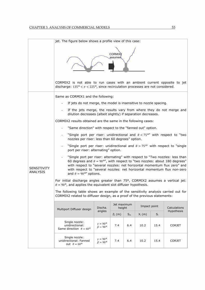
CHAPTER 3. ANALYSIS OF COMMERCIAL MODELS 53
jet. The figure below shows a profile view of this case:
CORMIX2 is not able to run cases with an ambient current opposite to jet discharge: 135° 225°, since recirculation processes are not considered.
SENSITIVITY ANALYSIS
Same as CORMIX1 and the following:
- If jets do not merge, the model is insensitive to nozzle spacing.
- If the jets merge, the results vary from where they do not merge and dilution decreases (albeit slightly) if separation decreases.
CORMIX2 results obtained are the same in the following cases:
- "Same direction" with respect to the “fanned out" option.
- “Single port per riser: unidirectional and 75°” with respect to “two nozzles per riser: less than 60 degrees” option.
- “Single port per riser: unidirectional and 75°" with respect to “single port per riser: alternating” option.
- “Single port per riser: alternating” with respect to “Two nozzles: less than 60 degrees and 90°”, with respect to “two nozzles: about 180 degrees” with respect to “several nozzles: net horizontal momentum flux zero” and with respect to “several nozzles: net horizontal momentum flux non-zero and 90°” options.
For initial discharge angles greater than 75º, CORMIX2 assumes a vertical jet: 90°, and applies the equivalent slot diffuser hypothesis.
The following table shows an example of the sensitivity analysis carried out for CORMIX2 related to diffuser design, as a proof of the previous statements:
Multiport Diffuser design Discha. angles
Jet maximum height
Impact point Calculations Hypothesis
Zt (m) Sm Xi (m) Si
Single nozzle: unidirectional:
Same direction 60°
90° 90° 7.4 6.4 10.2 15.4 CORJET
Single nozzle: unidirectional: Fanned
out 60°
90° 90° 7.4 6.4 10.2 15.4 CORJET
CORMIX2 assumes:

54 CHAPTER 3. ANALYSIS OF COMMERCIAL MODELS
In the case of interaction between jets, the results are less sensitive to the initial jet discharge angle, since the following simplification is made: if 45° 0°; and if 45° 90°).
Two nozzles: less than 60º
Same direction/ fanned out
90° 90° 7.4 6.4 10.2 15.4 CORJET
X (m) S BH BV
Single nozzle: unidirectional
Same direction/ fanned out
90° 1.5 9.7 75.5 0.45 Equivalent
slot diffuser.
Single nozzle: unidirectional
Same direction/ fanned out
90 1.5 9.7 75.5 0.45 Equivalent slot diffuser
Single nozzle: alternating Same direction/ fanned
out - 1.5 9.7 75.5 0.45
Equivalent slot diffuser
Two nozzles: less than 60º Same
direction/fanned out 90 1.87 7.7 75.5 0.6
Equivalent slot diffuser
Two nozzles: about 180º Same direction/ fanned
out - 1.87 7.7 75.5 0.6
Equivalent slot diffuser
Several nozzles: net horizontal momentum
flux zero (3ports) Same direction// fanned
out
- 2.1 6.7 75.5 0.65 Equivalent slot diffuser
VALIDATION BY SOFTWARE AUTHORS
Significant lack of validation studies from the software authors for negatively buoyant effluents.
Validation is limited to the case of a unilateral diffuser with vertical jets in a homogeneous and dynamic water receiving body. Validation is restricted to jet paths, but not dilution rates.
No validation is offered for the slot equivalent diffuser and other assumptions.
MODEL RESULTS RELIABILITY
Same as CORMIX1 and the following:
Considering the severe simplifications in the diffuser design, CORMIX2 does not provide a reliable modelling of the following cases: “single port per riser: unidirectional and 75°” “one single port per riser: alternating”, “two ports per riser: about 180º or less than 60º and 90°”, several nozzles: net horizontal momentum flux non-zero and 90°” and “several nozzles: net horizontal momentum flux zero”
CHAPTER 3. ANALYSIS OF COMMERCIAL MODELS 55
Table 3.3. Main CORMIX2 features related to brine discharge modeling
RECOMMENDATIONS
Same as CORMIX1 and the following:
- For the modelling of a “diffuser with one nozzle per riser and alternating jets”, or “two nozzles per riser forming 180”, it is recommended to model each diffuser side independently, as “one nozzle per riser: unidirectional” diffuser. This recommendation would avoid CORMIX2, applying the simplification of a single vertical jet, which is not correct for negatively buoyant jets.
- Since there is no validation for the slot equivalent diffuser hypothesis in the case of dense jets and merging decreases dilution, it is recommended to design the nozzles sufficiently separated to avoid interaction between jets.
With respect to the diffuser design:
- For the design of a diffuser parallel to the coast (and to the ambient current), the “single nozzles per riser: unidirectional: same direction” option is recommended with the following input data: 90°;
270° (or 90° if it is discharged towards the coast), 0° and 45° 60°. In this case the distance from the coast to the diffuser
nearest point (YB1) is equal to the distance from the coast to the farthest away point (YB2): YB1=YB2.
- For the design of a diffuser perpendicular to the coast (and to the ambient current), the “single nozzles per riser: unidirectional: same direction” option is recommended with the following input data:
90°, 0°, 90° and 45° 60°. In this case the distance to the nearest and farthest away point are related with the formula: YB1=Ld+YB2, Ld being the diffuser length.

56 CHAPTER 3. ANALYSIS OF COMMERCIAL MODELS
3.3.3. CORJET, UM3 and JETLAG: Commercial models based on the integration of differential equations
CORJET
(CORMIX) UM3
(VISUAL PLUMES) JETLAG (VISJET)
ACCESS Commercial model Free access model.
EPA web site. Commercial model
APPLICATION
Positively and negatively buoyant effluents.
Single and multiport submerged jet discharges.
Near field models.
MODELLING APPROACH
Eulerian approach.
Models based on the integration of the motion and transport differential equations through the cross section, transforming them into an ordinary equation system, which is solved using a simple numerical method (Runge-Kutta 4th order).
Lagragian approach.
The mathematical governing equations are not strictly solved, but an approximation of the physical processes, considering entrainment is made.
MAIN ASSUMPTIONS
Unlimited environment.
Self-similarity cross-sectional profiles. Round section for jets.
Stationary state.
Simple entrainment models based on the eddy viscosity concept.
Gaussian profiles. The results are referred to the jet centerline.
“Entrainment” model based on the Priestly et al. (1955) formula for round vertical jets. A term for inclination effects is included: sin .
For merging between jets, the hypothesis of an equivalent slot diffuser is applied while conserving the fluxes.
Origin (xo, yo): at the jet nozzle (centerline), and (zo): at the bottom.
CORJET is strictly valid only for the five asymptotic self similar regimes. In, other cases, it uses an approximation.
Top Hat (uniform) jet profiles.
The results refer to the average values of the cross section.
The generalized 3D Projected-area-entrainment (PAE) hypothesis, quantifying the mass incorporated into the plume in the presence of a current including the effect of a cross current.
Dilution from diffusers oriented parallel to the current is estimated by limiting the effective spacing to correspond to a cross-diffuser flow angle of 20º.
The “entrainment” is based on the Projected-area-entrainment (PAE) hypothesis and includes terms for the effect of the jet excess of velocity and the presence of a cross (transverse) ambient current, Roberts et al. (1987).
Origin (xo,yo,zo) at the jet nozzle (centerline).
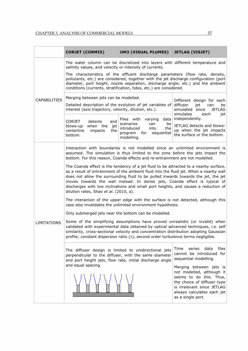
CHAPTER 3. ANALYSIS OF COMMERCIAL MODELS 57
CORJET (CORMIX) UM3 (VISUAL PLUMES) JETLAG (VISJET)
CAPABILITIES
The water column can be discretized into layers with different temperature and salinity values, and velocity or intensity of currents.
The characteristics of the effluent discharge parameters (flow rate, density, pollutants, etc.) are considered, together with the jet discharge configuration (port diameter, port height, nozzle separation, discharge angle, etc.) and the ambient conditions (currents, stratification, tides, etc.) are considered.
Merging between jets can be modelled.
Detailed description of the evolution of jet variables of interest (axis trajectory, velocity, dilution, etc.).
Different design for each diffuser jet can be simulated since JETLAG simulates each jet independently.
JETLAG detects and blows-up when the jet impacts the surface or the bottom.
CORJET detects and blows-up when the jet centerline impacts the bottom.
Files with varying data scenarios can be introduced into the program for sequential modelling.
LIMITATIONS
Interaction with boundaries is not modelled since an unlimited environment is assumed. The simulation is thus limited to the zone before the jets impact the bottom. For this reason, Coanda effects and re-entrainment are not modelled.
The Coanda effect is the tendency of a jet fluid to be attracted to a nearby surface, as a result of entrainment of the ambient fluid into the fluid jet. When a nearby wall does not allow the surrounding fluid to be pulled inwards towards the jet, the jet moves towards the wall instead. In dense jets, Coanda effect is typical of discharges with low inclinations and small port heights, and causes a reduction of dilution rates, Shao et al. (2010, a).
The interaction of the upper edge with the surface is not detected, although this case also invalidates the unlimited environment hypothesis.
Only submerged jets near the bottom can be modelled.
Some of the simplifying assumptions have proved unrealistic (or invalid) when validated with experimental data obtained by optical advanced techniques, i.e. self similarity, cross-sectional velocity and concentration distribution adopting Gaussian profile; constant dispersion ratio ( ), second order turbulence terms negligible.
The diffuser design is limited to unidirectional jets perpendicular to the diffuser, with the same diameter and port height jets, flow rate, initial discharge angle and equal spacing.
Time series data files cannot be introduced for sequential modelling.
Merging between jets is not modelled, although it seems to do this. Thus, the choice of diffuser type is irrelevant since JETLAG always calculates each jet as a single port.

58 CHAPTER 3. ANALYSIS OF COMMERCIAL MODELS
CORJET (CORMIX) UM3 (VISUAL PLUMES) JETLAG (VISJET)
SENSITIVITY ANALYSIS
Considering the range of real data on ambient conditions in the Western Mediterranean and the range of actual values for brine discharge design, the results from these models are especially sensitive to these variables:
- Initial Discharge angle with respect to the bottom ( ) and discharge velocity.
- Ambient current intensity: faster, greater dilution.
Results in all three models are insensitive to the water column depth if the jets do not impact the surface, and insensitive to the separation between jets if there is no merging.
Maximum dilutions at the impact point for initial discharge angles between 45º-60º.
Not very sensitive to port height.
With respect to the ambient current direction, CORJET dilution results are almost insensitive to this parameter.
If merging occurs, sensitivity to the separation between nozzles remains very low.
Maximum dilution at the impact point for a 60º initial discharge angle.
Insensitive to port height.
Low sensitivity to ambient current directions with respect to the jet. Slightly higher dilutions are obtained for cross (transverse) currents.
If merging occurs, sensitivity to the separation between nozzles remains very low.
Maximum dilution at the impact point for an initial discharge angle of 60º.
Insensitive to port height.
With respect to the ambient current direction, higher dilution is obtained for transverse currents and lower dilution rates for counter-flowing (opposing) and co-flowing (parallel) currents.
Insensitive to the separation between ports, since each jet is modelled independently.
VALIDATION BY SOFTWARE AUTHORS
Lack of validation studies presented by the software authors for negatively buoyant jets.
Hypotheses formulated for the merging process have not been validated for inclined dense jets.
Validation limited to the jet path and solely in the case of vertical jets discharging into a dynamic and homogeneous environment.
Validation limited to a stagnant and homogeneous environment. Validation limited to the jet path, with very limited data for dilution rates, Jirka (2008).
No validation data have been found for negatively buoyant effluents.
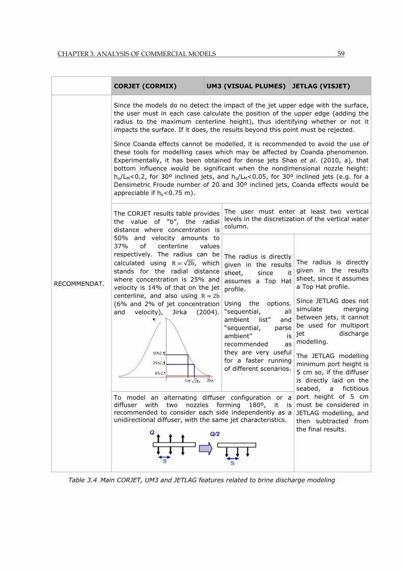
CHAPTER 3. ANALYSIS OF COMMERCIAL MODELS 59
Table 3.4. Main CORJET, UM3 and JETLAG features related to brine discharge modeling
CORJET (CORMIX) UM3 (VISUAL PLUMES) JETLAG (VISJET)
RECOMMENDAT.
Since the models do no detect the impact of the jet upper edge with the surface, the user must in each case calculate the position of the upper edge (adding the radius to the maximum centerline height), thus identifying whether or not it impacts the surface. If it does, the results beyond this point must be rejected.
Since Coanda effects cannot be modelled, it is recommended to avoid the use of these tools for modelling cases which may be affected by Coanda phenomenon. Experimentally, it has been obtained for dense jets Shao et al. (2010, a), that bottom influence would be significant when the nondimensional nozzle height: ho/LM<0.2, for 30º inclined jets, and ho/LM<0.05, for 30º inclined jets (e.g. for a Densimetric Froude number of 20 and 30º inclined jets, Coanda effects would be appreciable if ho<0.75 m).
The CORJET results table provides the value of “b”, the radial distance where concentration is 50% and velocity amounts to 37% of centerline values respectively. The radius can be calculated using R √2b, which stands for the radial distance where concentration is 25% and velocity is 14% of that on the jet centerline, and also using R 2b (6% and 2% of jet concentration and velocity), Jirka (2004).
The user must enter at least two vertical levels in the discretization of the vertical water column.
The radius is directly given in the results sheet, since it assumes a Top Hat profile.
Using the options. “sequential, all ambient list” and “sequential, parse ambient” is recommended as they are very useful for a faster running of different scenarios.
The radius is directly given in the results sheet, since it assumes a Top Hat profile.
Since JETLAG does not simulate merging between jets, it cannot be used for multiport jet discharge modelling.
The JETLAG modelling minimum port height is 5 cm so, if the diffuser is directly laid on the seabed, a fictitious port height of 5 cm must be considered in JETLAG modelling, and then subtracted from the final results.
To model an alternating diffuser configuration or a diffuser with two nozzles forming 180º, it is recommended to consider each side independently as a unidirectional diffuser, with the same jet characteristics.
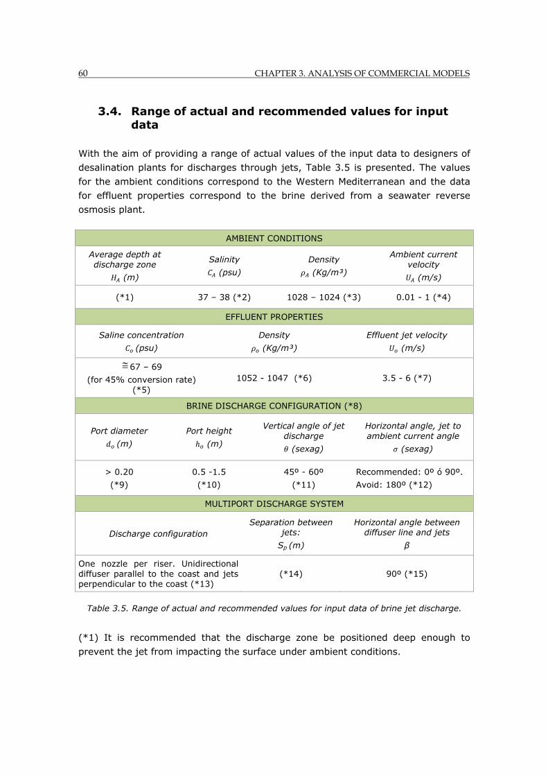
60 CHAPTER 3. ANALYSIS OF COMMERCIAL MODELS
3.4. Range of actual and recommended values for input data
With the aim of providing a range of actual values of the input data to designers of
desalination plants for discharges through jets, Table 3.5 is presented. The values
for the ambient conditions correspond to the Western Mediterranean and the data
for effluent properties correspond to the brine derived from a seawater reverse
osmosis plant.
Table 3.5. Range of actual and recommended values for input data of brine jet discharge.
(*1) It is recommended that the discharge zone be positioned deep enough to
prevent the jet from impacting the surface under ambient conditions.
AMBIENT CONDITIONS
Average depth at discharge zone
(m)
Salinity
(psu)
Density
(Kg/m³)
Ambient current velocity
(m/s)
(*1) 37 – 38 (*2) 1028 – 1024 (*3) 0.01 - 1 (*4)
EFFLUENT PROPERTIES
Saline concentration
(psu)
Density
(Kg/m³)
Effluent jet velocity
(m/s)
67 – 69
(for 45% conversion rate) (*5)
1052 - 1047 (*6) 3.5 - 6 (*7)
BRINE DISCHARGE CONFIGURATION (*8)
Port diameter
(m)
Port height
(m)
Vertical angle of jet discharge
(sexag)
Horizontal angle, jet to ambient current angle
(sexag)
> 0.20
(*9)
0.5 -1.5
(*10)
45º - 60º
(*11)
Recommended: 0º ó 90º.
Avoid: 180º (*12)
MULTIPORT DISCHARGE SYSTEM
Discharge configuration Separation between
jets:
Sp (m)
Horizontal angle between diffuser line and jets
β
One nozzle per riser. Unidirectional diffuser parallel to the coast and jets perpendicular to the coast (*13)
(*14) 90º (*15)
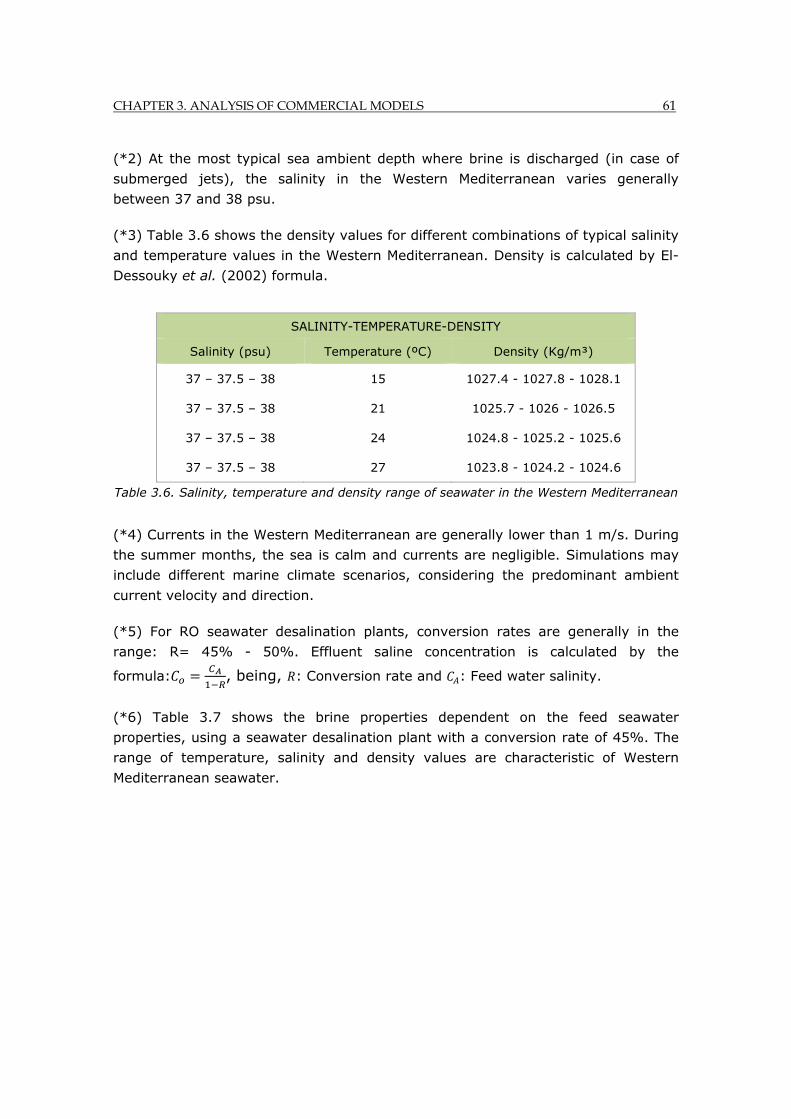
CHAPTER 3. ANALYSIS OF COMMERCIAL MODELS 61
(*2) At the most typical sea ambient depth where brine is discharged (in case of
submerged jets), the salinity in the Western Mediterranean varies generally
between 37 and 38 psu.
(*3) Table 3.6 shows the density values for different combinations of typical salinity
and temperature values in the Western Mediterranean. Density is calculated by El-
Dessouky et al. (2002) formula.
Table 3.6. Salinity, temperature and density range of seawater in the Western Mediterranean
(*4) Currents in the Western Mediterranean are generally lower than 1 m/s. During
the summer months, the sea is calm and currents are negligible. Simulations may
include different marine climate scenarios, considering the predominant ambient
current velocity and direction.
(*5) For RO seawater desalination plants, conversion rates are generally in the
range: R= 45% - 50%. Effluent saline concentration is calculated by the
formula: , being, : Conversion rate and : Feed water salinity.
(*6) Table 3.7 shows the brine properties dependent on the feed seawater
properties, using a seawater desalination plant with a conversion rate of 45%. The
range of temperature, salinity and density values are characteristic of Western
Mediterranean seawater.
SALINITY-TEMPERATURE-DENSITY
Salinity (psu) Temperature (ºC) Density (Kg/m³)
37 – 37.5 – 38 15 1027.4 - 1027.8 - 1028.1
37 – 37.5 – 38 21 1025.7 - 1026 - 1026.5
37 – 37.5 – 38 24 1024.8 - 1025.2 - 1025.6
37 – 37.5 – 38 27 1023.8 - 1024.2 - 1024.6
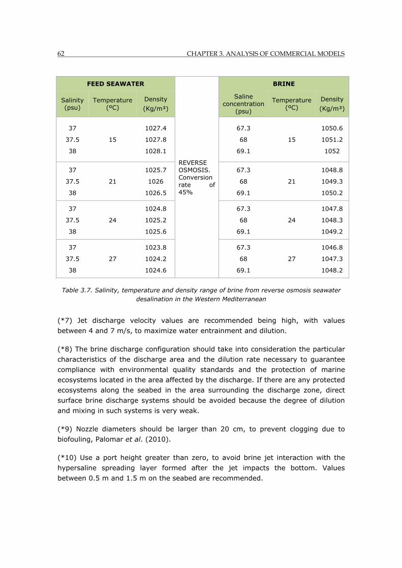
62 CHAPTER 3. ANALYSIS OF COMMERCIAL MODELS
Table 3.7. Salinity, temperature and density range of brine from reverse osmosis seawater desalination in the Western Mediterranean
(*7) Jet discharge velocity values are recommended being high, with values
between 4 and 7 m/s, to maximize water entrainment and dilution.
(*8) The brine discharge configuration should take into consideration the particular
characteristics of the discharge area and the dilution rate necessary to guarantee
compliance with environmental quality standards and the protection of marine
ecosystems located in the area affected by the discharge. If there are any protected
ecosystems along the seabed in the area surrounding the discharge zone, direct
surface brine discharge systems should be avoided because the degree of dilution
and mixing in such systems is very weak.
(*9) Nozzle diameters should be larger than 20 cm, to prevent clogging due to
biofouling, Palomar et al. (2010).
(*10) Use a port height greater than zero, to avoid brine jet interaction with the
hypersaline spreading layer formed after the jet impacts the bottom. Values
between 0.5 m and 1.5 m on the seabed are recommended.
FEED SEAWATER
REVERSE OSMOSIS. Conversion rate of 45%
BRINE
Salinity (psu)
Temperature (ºC)
Density
(Kg/m³)
Saline concentration
(psu)
Temperature (ºC)
Density
(Kg/m³)
37
37.5
38
15
1027.4
1027.8
1028.1
67.3
68
69.1
15
1050.6
1051.2
1052
37
37.5
38
21
1025.7
1026
1026.5
67.3
68
69.1
21
1048.8
1049.3
1050.2
37
37.5
38
24
1024.8
1025.2
1025.6
67.3
68
69.1
24
1047.8
1048.3
1049.2
37
37.5
38
27
1023.8
1024.2
1024.6
67.3
68
69.1
27
1046.8
1047.3
1048.2
CHAPTER 3. ANALYSIS OF COMMERCIAL MODELS 63
(*11) Use an initial discharge angle between 45º and 60º in a predominantly
stagnant and homogeneous environment, as these have been experimentally
proven to be the most effective angles with respect to dilution. In the case of
significant currents with different directions, vertical jets (90º) achieve higher
dilution rates, Roberts et al. (1987).
(*12) Experimental investigations, Roberts et al. (1987) have revealed that co-
flowing and transverse currents increase brine discharge dilution, while counter-
flowing currents reduce dilution.
(*13) Avoid designs with several jets in a rosette and alternating diffusers since the
extensive spreading layer beyond the impact point tends to overflow the diffusers.
(*14) Use riser spacing large enough to avoid merging between contiguous jets
along the trajectory since this interaction reduces the dilution obtained in the near
field region. Furthermore, the commercial modeling tools have not been validated
for the merging of negatively buoyant inclined jets and consequently, present
uncertainties in these predictions.
(*15) Position jets perpendicular to the diffuser line.
3.5. Conclusions
As a predictive tool of the flow behavior, numerical modeling is a fundamental tool
in environmental impact assessment of brine discharges.
CORMIX, VISUAL PLUMES and VISJET software have been identified as the most
used commercial models to simulate brine discharges. They have been widely used
in the design of discharge configurations in Spanish and worldwide desalination
plants. However, these models have not been submitted to a critical analysis when
simulating this type of negatively buoyant effluents, presenting significant
uncertainties that required to be contrasted.
To overcome this knowledge gap and to obtain a better knowledge of the
theoretical basis and the application of these models to brine discharge, an
exhaustive analysis has been carried out in the present chapter. The analysis has
included the following information: modeling approach, simplifying assumptions,
capabilities, limitations, sensitivity analysis and validation by model authors.
Specific recommendations for each model have been provided in section 3.3,
regarding their use and application.
64 CHAPTER 3. ANALYSIS OF COMMERCIAL MODELS
From this work, the following conclusions and recommendations for the use of
commercial tools for brine discharge modeling can be formulated:
- For single port jet discharges, the use of integral models, such as CORJET, UM3 and JETLAG is recommended rather than the CORMIX1 and CORMIX2 subsystems, as they (CORMIX1 and CORMIX2) use very simplified formulas and have not been validated for negatively buoyant discharges. Some significant errors have been detected in their flow classification. An alternative is the use of the length scales formulas calibrated and validated in the literature, with experimental data for hyperdense inclined jets, but these formulas only characterize geometry and dilution at specific control points.
- Models based on the integration of differential equations are not recommended for initial discharge angles (relative to the bottom) under 30º and over 75º, since Coanda and re-entrainment respectively are not taken into account.
- When using CORJET, UM3 or JETLAG, the user must check in every case if the jet upper edge impacts the surface since the models do not detect such impacts.
- Significant errors have been detected in the sensitivity analysis carried out, related to the influence of ambient current direction. Commercial models seem not to follow the trend of experimental results published by Roberts et al. (1987). Some of the models are almost insensitive to ambient current direction.
- Regarding the reliability of the commercial models for multiport jet discharges:
o Users must take into account that the JETLAG model does not consider the interaction between jets and always calculates them independently, as single port jets. CORJET and UM3 take merging into account, but no validation studies of merging hypotheses have been found in the literature for inclined hyperdense effluents.
o Although CORMIX2 offers multiple possibilities for multiport diffuser configuration, important assumptions are made which invalidate its results for dense jets. A detailed description of this problem is made in the “limitations” and “recommendations” of CORMIX2 analysis (section 3.3.1).

CHAPTER 3. ANALYSIS OF COMMERCIAL MODELS 65
- Numerical tools need to be developed for modelling other discharge configurations which may be suitable in some cases, such as direct surface discharge, over-spill in a cliff, etc. Experimental data are necessary to calibrate, test and validate these tools.
- A common shortcoming of the commercial models analyzed is the lack of validation studies for negatively buoyant jets, such as those typical of brine discharges. To investigate and determine the degree of agreement of commercial tools for near field brine discharge modelling, next chapter presents a detailed validation of their numerical results with experimental data, including stagnant and dynamic environments.

66 CHAPTER 3. ANALYSIS OF COMMERCIAL MODELS
CHAPTER 4. VALIDATION OF COMMERCIAL MODELS 67
Chapter 4. VALIDATION OF COMMERCIAL TOOLS FOR BRINE DISCHARGES
Chapter 4 VALIDATION OF COMMERCIAL MODELS FOR BRINE DISCHARGES
Summary
Chapter 3 has presented a detailed analysis of the commercial models CORMIX,
VISUAL PLUMES and VISJET software, widely used for modeling brine discharges.
This chapter completes the analysis, including an exhaustive validation of these
commercial tools, using published experimental data from various authors.
According to the previous analysis, the validation focuses on submerged negatively
buoyant jets discharged into both, stagnant and dynamic environments. An
estimation of the discrepancies between these model results and experimental data
for different discharge designs is also included.
Conclusions and recommendations are provided describing the reliability and
accuracy of the commercial models in simulation of brine discharges. This intends
to be useful for reducing the uncertainty regarding the use of commercial models
for the simulation of brine discharges.
68 CHAPTER 4. VALIDATION OF COMMERCIAL MODELS
4.1. Introduction
According to the analysis carried out in Chapter 3, a common shortcoming of
commercial models is the lack of validation studies provided by the software
developers for negatively buoyant effluents, such as brine.
In particular, no validation studies for this type of effluent have been provided for
CORMIX1 and CORMIX2 subsystems, while CORJET module validation is limited to
the case of an inclined jet discharged into a stagnant and homogeneous
environment, and mainly for jet geometry, with very little data on dilution rates,
Jirka (2008). Regarding the UM3 model of VISUAL PLUMES, to our knowledge, no
validation data have been published by the developers for hyperdense jets. With
respect to the JETLAG model, included as a part of the VISJET software, the
validation provided by the developers is limited to the jet path, and only for the
case of a vertical jet discharged into a dynamic and homogeneous environment,
Lee et al. (1990).
With the aim of remedying these shortcomings and reducing the uncertainty in the
use of these models for simulating brine discharges, a validation with experimental
data has been carried out and is presented in this chapter. The validation focuses
on a single port submerged brine jet discharges into stagnant and dynamic
environments. Numerical results obtained by CORMIX1, CORJET, UM3 and JETLAG
models have been compared with the experimental data found in literature,
including the geometry, dilution and velocity of brine jet discharges.
The present chapter is organized as follows: A selection and description of the most
important experimental data found in the literature for inclined dense jets
discharged into a stagnant and dynamic environment is first outlined. Next, the
validation of the commercial models with experimental data, including graphs, and
a qualitative and quantitative analysis are presented. Finally, conclusions relating to
the accuracy and reliability of the commercial models for near field brine modeling
are drawn, and future research lines are postulated.
4.2. Experimental data selected for commercial models validation
Experimental physical modeling consists of small-scale experiments run in the
laboratory under controlled conditions. The model and the prototype maintain their
relative proportions and they are scaled in terms of both geometry and forces.
Geometric and kinematic similarities are guaranteed by scaling magnitudes in the
CHAPTER 4. VALIDATION OF COMMERCIAL MODELS 69
model and the prototype, and dynamic similarity is considered achieved when the
Densimetric Froude number (a nondimensional parameter measuring the ratio of
the inertial force to the gravitational force) remains the same in both the prototype
and the model. A high Reynolds number (Re> 2000), Jirka (2004), is required to
ensure a fully turbulent flow in single round jets.
Experimental data are needed to validate numerical models. Traditionally,
laboratory measurements have been carried out with intrusive techniques, which
can alter the flow characteristics. More recently, sophisticated optical techniques
have been incorporated in brine discharge studies, such as Laser Induced
Fluorescence (LIF) and Particle Image Velocimetry (PIV), which characterize the
concentration and velocity fields in time and space with a high degree of detail.
The following sections describe the experimental studies available in the literature
carried out to characterize negatively buoyant jets.
4.2.1. Experimental data for an inclined dense jet discharged into a stagnant environment
Regarding the case of a single port dense jet discharged into an unlimited,
homogeneous and stagnant environment, various experimental studies have been
developed in recent years.
In most cases, experimental results have been used by authors for calibrating
dimensional analysis formulas, which characterize the brine behavior in specific
points of the jet path. The dimensional analysis for round jets into a stagnant and
homogeneous ambient, assuming a full turbulent flow and Boussinesq hypothesis
for gravity terms, concludes that, for a specific initial discharge angle ( ), the jet
geometric features ( , ) and dilution rates ( ) mainly depend on the port
diameter ( ) and the Densimetric Froude number ( ), Fisher (1979).
Geometric features and dilution = , , 4.1
For a single port dense negatively buoyant jet, the following nondimensional
parameters are commonly calibrated (obtaining for each specific discharge angle,
) to characterize the flow at some specific points (i.e. maximum rise height and
impact with the bottom point):
; ; ; ; ; ; ; , . 4.2

70 CHAPTER 4. VALIDATION OF COMMERCIAL MODELS
Where:
: Maximum rise height (maximum height of the upper edge of the jet).
: Vertical location of the centerline peak.
: Horizontal location of the centerline peak.
: Centerline dilution at the centerline peak point.
: Horizontal location of the return point (location where the jet axis reaches the
port height level in the jet descending path).
: Centerline dilution at the return point.
: Horizontal location of the impact point (location where the jet axis impacts the
bottom).
: Centerline dilution at the impact point.
: Dimensional analysis coefficients experimentally obtained.
The origin of the coordinate system is taken to be the center of the nozzle. All
variables are referred to the jet during the steady state operation.
To illustrate these variables characterizing brine jet discharges, Figures 4.1 and 4.2
show a scheme of an inclined dense jet.
Figure 4.1. Variables at the singular points of an inclined dense jet. Profile view
X
Xi, Si Xm
Xr, Sr
Zt
Zm
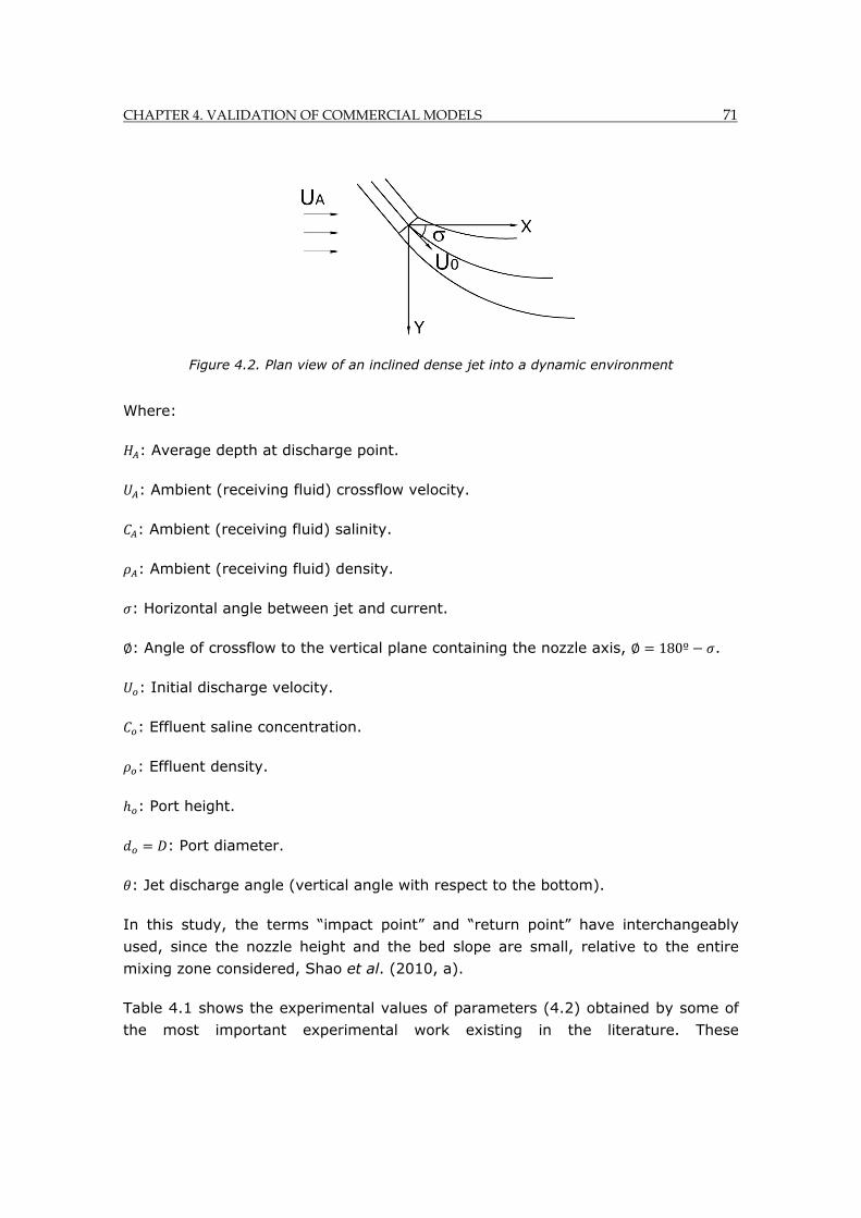
CHAPTER 4. VALIDATION OF COMMERCIAL MODELS 71
Figure 4.2. Plan view of an inclined dense jet into a dynamic environment
Where:
: Average depth at discharge point.
: Ambient (receiving fluid) crossflow velocity.
: Ambient (receiving fluid) salinity.
: Ambient (receiving fluid) density.
: Horizontal angle between jet and current.
: Angle of crossflow to the vertical plane containing the nozzle axis, 180º .
: Initial discharge velocity.
: Effluent saline concentration.
: Effluent density.
: Port height.
: Port diameter.
: Jet discharge angle (vertical angle with respect to the bottom).
In this study, the terms “impact point” and “return point” have interchangeably
used, since the nozzle height and the bed slope are small, relative to the entire
mixing zone considered, Shao et al. (2010, a).
Table 4.1 shows the experimental values of parameters (4.2) obtained by some of
the most important experimental work existing in the literature. These
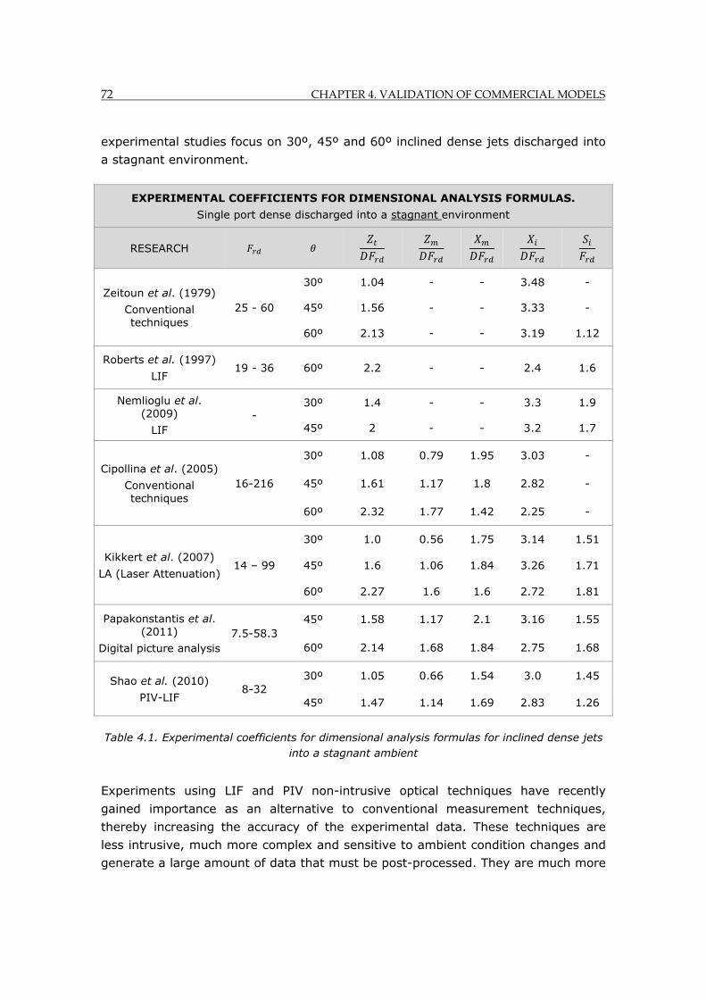
72 CHAPTER 4. VALIDATION OF COMMERCIAL MODELS
experimental studies focus on 30º, 45º and 60º inclined dense jets discharged into
a stagnant environment.
Table 4.1. Experimental coefficients for dimensional analysis formulas for inclined dense jets into a stagnant ambient
Experiments using LIF and PIV non-intrusive optical techniques have recently
gained importance as an alternative to conventional measurement techniques,
thereby increasing the accuracy of the experimental data. These techniques are
less intrusive, much more complex and sensitive to ambient condition changes and
generate a large amount of data that must be post-processed. They are much more
EXPERIMENTAL COEFFICIENTS FOR DIMENSIONAL ANALYSIS FORMULAS.
Single port dense discharged into a stagnant environment
RESEARCH
Zeitoun et al. (1979)
Conventional techniques
25 - 60
30º 1.04 - - 3.48 -
45º 1.56 - - 3.33 -
60º 2.13 - - 3.19 1.12
Roberts et al. (1997)
LIF 19 - 36 60º 2.2 - - 2.4 1.6
Nemlioglu et al. (2009)
LIF -
30º 1.4 - - 3.3 1.9
45º 2 - - 3.2 1.7
Cipollina et al. (2005)
Conventional techniques
16-216
30º 1.08 0.79 1.95 3.03 -
45º 1.61 1.17 1.8 2.82 -
60º 2.32 1.77 1.42 2.25 -
Kikkert et al. (2007)
LA (Laser Attenuation) 14 – 99
30º 1.0 0.56 1.75 3.14 1.51
45º 1.6 1.06 1.84 3.26 1.71
60º 2.27 1.6 1.6 2.72 1.81
Papakonstantis et al. (2011)
Digital picture analysis 7.5-58.3
45º 1.58 1.17 2.1 3.16 1.55
60º 2.14 1.68 1.84 2.75 1.68
Shao et al. (2010)
PIV-LIF 8-32
30º 1.05 0.66 1.54 3.0 1.45
45º 1.47 1.14 1.69 2.83 1.26
CHAPTER 4. VALIDATION OF COMMERCIAL MODELS 73
reliable for turbulent flows, as they measure the evolution of spatial and temporal
variables and are able to capture small scale motions that greatly affect flow driven
processes, such as entrainment and momentum damping. These features taken
together make optical techniques preferable for quantitative descriptions of the flow
and for numerical model calibration.
The calibrated formulas from the studies of: Roberts et al. (1997), Kikkert et al.
(1997), Shao et al. (2010) and Papakonstantis et al. (2011, a, b) have been
selected in the present work to validate the numerical results from commercial
tools.
4.2.2. Experimental data for an inclined dense jet discharged into a dynamic environment
Very few experimental investigations have been found in the literature for a single
port dense jet discharged into a dynamic environment. In this type of environment,
the jet behavior also depends on the ambient current velocity and direction relative
to the jet. Coflowing current expression refers to ambient crossflow parallel to the
jet at the discharge, whereas counter-flowing refers to ambient currents with the
same direction, but opposing to the jet at the discharge. Finally, transverse
currents are perpendicular to the jet at the discharge.
The dimensional analysis for negatively buoyant round jets into a dynamic
environment concludes that, for a specific initial discharge angle ( ), the jet
geometric features and dilution rates mainly depend on the port diameter ( ), the
Densimetric Froude number ( ), the ambient crossflow velocity ( ), the discharge
velocity ( ) and the horizontal angle of the jet with respect to the ambient current
( ):
Geometric features and dilution = , , , , , where . (4.3)
Dimensional analysis requires assuming a fully turbulent flow and the Boussinesq
hypothesis for gravity terms.
Regarding the experimental research available, Pincince et al. (1973) tested a 60º
inclined dense jet in a coflowing current ( 0°, 180°); Chu et al. (1975)
provided some laws for vertical dense jets ( 90°) discharged into a crossflow and
Tong et al. (1979) carried out experiments with 45º and 60º inclined jets
perpendicular to the crossflow.
74 CHAPTER 4. VALIDATION OF COMMERCIAL MODELS
Roberts et al. (1987) carried out important research for 90º and 60º inclined jets
discharged into a uniform crossflow of various speeds ( ) and directions ( ). The
test range was limited to 0< <1.87 and 12< <26 values. They measured the
following geometrical features and dilution rates: terminal rise height ( ;
minimum dilution at the terminal rise height ( ) and minimum dilution at the
impact point ( ).
Gungor et al. (2009) designed a new experiment for vertical jets in a crossflow,
using optical techniques, with tests limited to the 0.21< <0.91 range. The
same variables used by Roberts et al. (1987) were re-calibrated along with the
variable (horizontal location of the impact point) for the case of vertical jets.
Different laws, obtained by fitting experimental data, have been provided by the
previously mentioned authors. Among the experimental studies listed above,
Roberts et al. (1987) and Gungor et al. (2009) have been selected in this work for
the validation of the commercial models since the first includes a large quantity of
experiments and the second uses advanced LIF optical techniques. The laws
proposed by these authors have the following expressions:
0.2 0.8 4.4
0.8 4.5
/ 4.6
/ 4.7
where , , are the experimental coefficients obtained by fitting experimental
data.
Gungor et al. (2009) also includes an expression for the horizontal location of the
impact point:
4.8
Although Roberts et al. (1987) only published formulas for 90º and 60º inclined jets
perpendicular to the crossflow ( 90°), their experiments were carried out for a
huge variety of crossflow directions, including: 180°, 150°, 120°, 90°, 60°, 30°, 0°. With
the aim of making the most of Roberts et al.´s experiments, all their data have
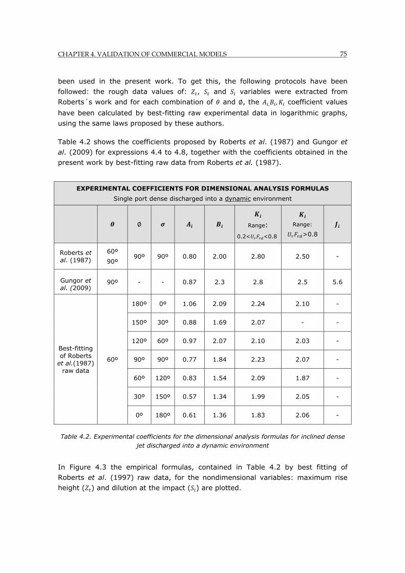
CHAPTER 4. VALIDATION OF COMMERCIAL MODELS 75
been used in the present work. To get this, the following protocols have been
followed: the rough data values of: , and variables were extracted from
Roberts´s work and for each combination of and , the , , coefficient values
have been calculated by best-fitting raw experimental data in logarithmic graphs,
using the same laws proposed by these authors.
Table 4.2 shows the coefficients proposed by Roberts et al. (1987) and Gungor et
al. (2009) for expressions 4.4 to 4.8, together with the coefficients obtained in the
present work by best-fitting raw data from Roberts et al. (1987).
Table 4.2. Experimental coefficients for the dimensional analysis formulas for inclined dense jet discharged into a dynamic environment
In Figure 4.3 the empirical formulas, contained in Table 4.2 by best fitting of
Roberts et al. (1997) raw data, for the nondimensional variables: maximum rise
height ( ) and dilution at the impact ( ) are plotted.
EXPERIMENTAL COEFFICIENTS FOR DIMENSIONAL ANALYSIS FORMULAS
Single port dense discharged into a dynamic environment
Range:
0.2< <0.8
Range:
>0.8
Roberts et al. (1987)
60º
90º 90º 90º 0.80 2.00 2.80 2.50 -
Gungor et al. (2009)
90º - - 0.87 2.3 2.8 2.5 5.6
Best-fitting of Roberts
et al.(1987) raw data
60º
180º 0º 1.06 2.09 2.24 2.10 -
150º 30º 0.88 1.69 2.07 - -
120º 60º 0.97 2.07 2.10 2.03 -
90º 90º 0.77 1.84 2.23 2.07 -
60º 120º 0.83 1.54 2.09 1.87 -
30º 150º 0.57 1.34 1.99 2.05 -
0º 180º 0.61 1.36 1.83 2.06 -
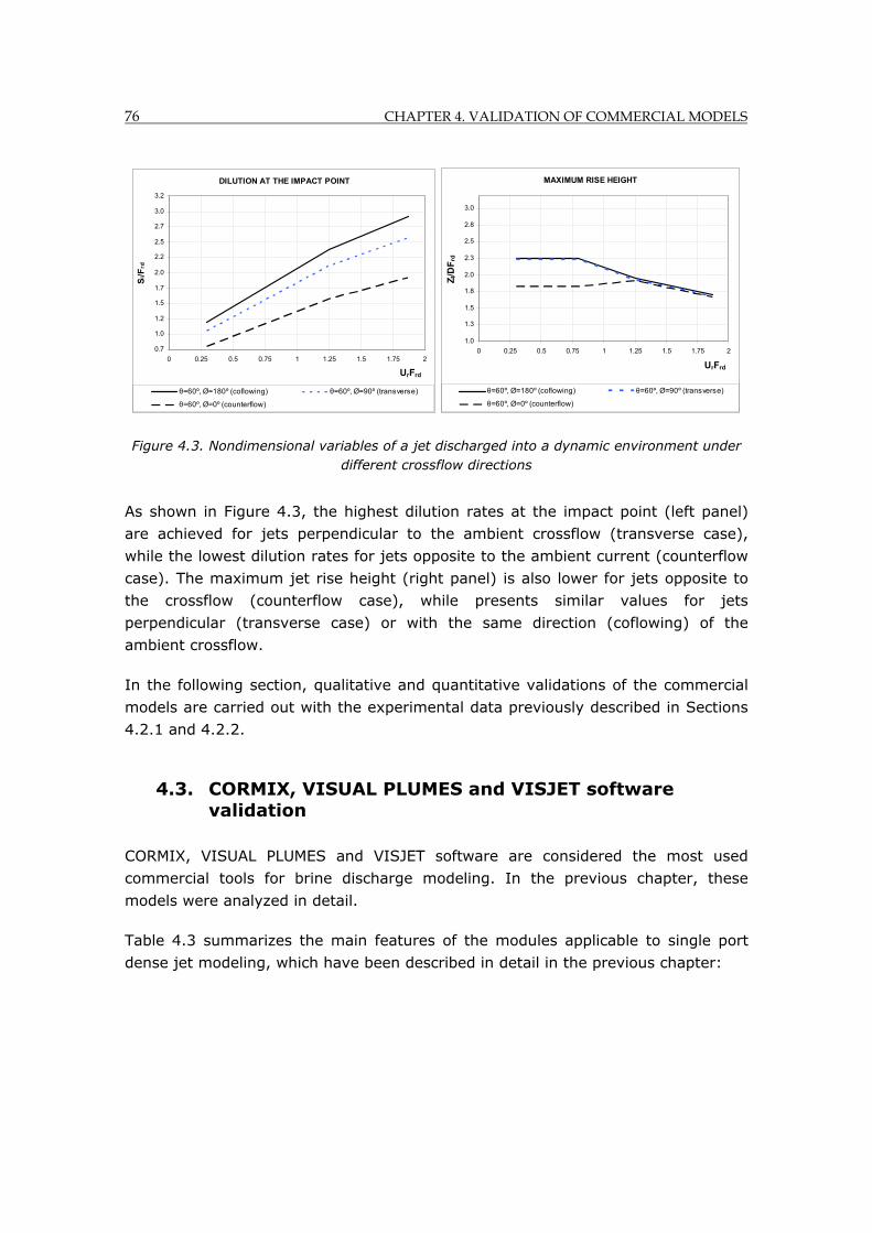
76 CHAPTER 4. VALIDATION OF COMMERCIAL MODELS
Figure 4.3. Nondimensional variables of a jet discharged into a dynamic environment under different crossflow directions
As shown in Figure 4.3, the highest dilution rates at the impact point (left panel)
are achieved for jets perpendicular to the ambient crossflow (transverse case),
while the lowest dilution rates for jets opposite to the ambient current (counterflow
case). The maximum jet rise height (right panel) is also lower for jets opposite to
the crossflow (counterflow case), while presents similar values for jets
perpendicular (transverse case) or with the same direction (coflowing) of the
ambient crossflow.
In the following section, qualitative and quantitative validations of the commercial
models are carried out with the experimental data previously described in Sections
4.2.1 and 4.2.2.
4.3. CORMIX, VISUAL PLUMES and VISJET software validation
CORMIX, VISUAL PLUMES and VISJET software are considered the most used
commercial tools for brine discharge modeling. In the previous chapter, these
models were analyzed in detail.
Table 4.3 summarizes the main features of the modules applicable to single port
dense jet modeling, which have been described in detail in the previous chapter:
DILUTION AT THE IMPACT POINT
0.7
1.0
1.2
1.5
1.7
2.0
2.2
2.5
2.7
3.0
3.2
0 0.25 0.5 0.75 1 1.25 1.5 1.75 2
UrFrd
Si/F
rd
θ=60º, Ø=180º (coflowing) θ=60º, Ø=90º (transverse)
θ=60º, Ø=0º (counterflow)
MAXIMUM RISE HEIGHT
1.0
1.3
1.5
1.8
2.0
2.3
2.5
2.8
3.0
0 0.25 0.5 0.75 1 1.25 1.5 1.75 2
UrFrd
Z t/D
Frd
θ=60º, Ø=180º (coflowing) θ=60º, Ø=90º (transverse)
θ=60º, Ø=0º (counterflow)
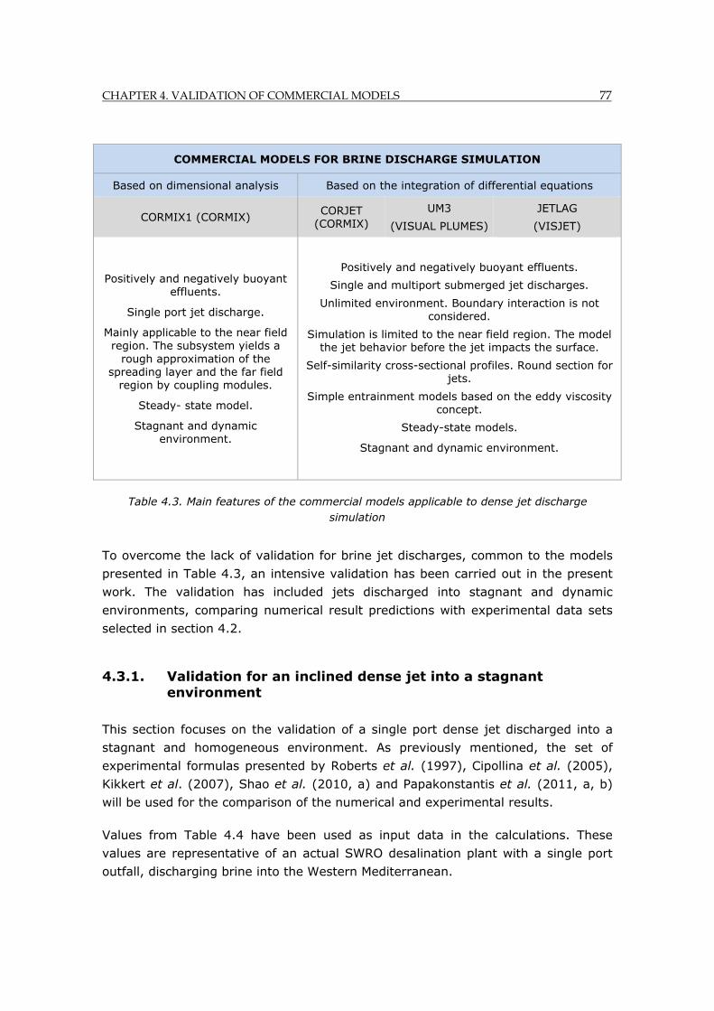
CHAPTER 4. VALIDATION OF COMMERCIAL MODELS 77
Table 4.3. Main features of the commercial models applicable to dense jet discharge simulation
To overcome the lack of validation for brine jet discharges, common to the models
presented in Table 4.3, an intensive validation has been carried out in the present
work. The validation has included jets discharged into stagnant and dynamic
environments, comparing numerical result predictions with experimental data sets
selected in section 4.2.
4.3.1. Validation for an inclined dense jet into a stagnant environment
This section focuses on the validation of a single port dense jet discharged into a
stagnant and homogeneous environment. As previously mentioned, the set of
experimental formulas presented by Roberts et al. (1997), Cipollina et al. (2005),
Kikkert et al. (2007), Shao et al. (2010, a) and Papakonstantis et al. (2011, a, b)
will be used for the comparison of the numerical and experimental results.
Values from Table 4.4 have been used as input data in the calculations. These
values are representative of an actual SWRO desalination plant with a single port
outfall, discharging brine into the Western Mediterranean.
COMMERCIAL MODELS FOR BRINE DISCHARGE SIMULATION
Based on dimensional analysis Based on the integration of differential equations
CORMIX1 (CORMIX) CORJET
(CORMIX) UM3
(VISUAL PLUMES)
JETLAG
(VISJET)
Positively and negatively buoyant effluents.
Single port jet discharge.
Mainly applicable to the near field region. The subsystem yields a
rough approximation of the spreading layer and the far field
region by coupling modules.
Steady- state model.
Stagnant and dynamic environment.
Positively and negatively buoyant effluents.
Single and multiport submerged jet discharges.
Unlimited environment. Boundary interaction is not considered.
Simulation is limited to the near field region. The model the jet behavior before the jet impacts the surface.
Self-similarity cross-sectional profiles. Round section for jets.
Simple entrainment models based on the eddy viscosity concept.
Steady-state models.
Stagnant and dynamic environment.
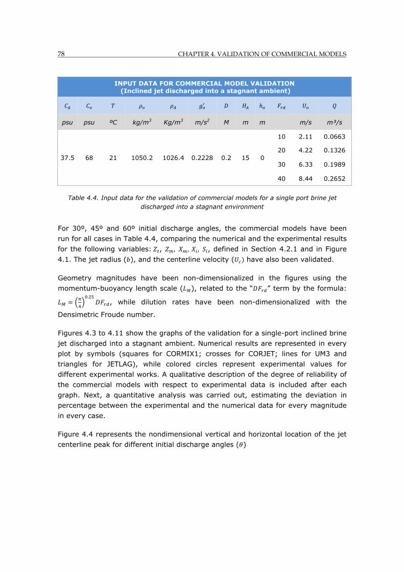
78 CHAPTER 4. VALIDATION OF COMMERCIAL MODELS
INPUT DATA FOR COMMERCIAL MODEL VALIDATION (Inclined jet discharged into a stagnant ambient)
psu psu ºC kg/m3 Kg/m3 m/s2 M m m m/s m³/s
37.5 68 21 1050.2 1026.4 0.2228 0.2 15 0
10 2.11 0.0663
20 4.22 0.1326
30 6.33 0.1989
40 8.44 0.2652
Table 4.4. Input data for the validation of commercial models for a single port brine jet discharged into a stagnant environment
For 30º, 45º and 60º initial discharge angles, the commercial models have been
run for all cases in Table 4.4, comparing the numerical and the experimental results
for the following variables: , , , , , defined in Section 4.2.1 and in Figure
4.1. The jet radius ( ), and the centerline velocity ( have also been validated.
Geometry magnitudes have been non-dimensionalized in the figures using the
momentum-buoyancy length scale ( ), related to the “ ” term by the formula: .
, while dilution rates have been non-dimensionalized with the
Densimetric Froude number.
Figures 4.3 to 4.11 show the graphs of the validation for a single-port inclined brine
jet discharged into a stagnant ambient. Numerical results are represented in every
plot by symbols (squares for CORMIX1; crosses for CORJET; lines for UM3 and
triangles for JETLAG), while colored circles represent experimental values for
different experimental works. A qualitative description of the degree of reliability of
the commercial models with respect to experimental data is included after each
graph. Next, a quantitative analysis was carried out, estimating the deviation in
percentage between the experimental and the numerical data for every magnitude
in every case.
Figure 4.4 represents the nondimensional vertical and horizontal location of the jet
centerline peak for different initial discharge angles ( )
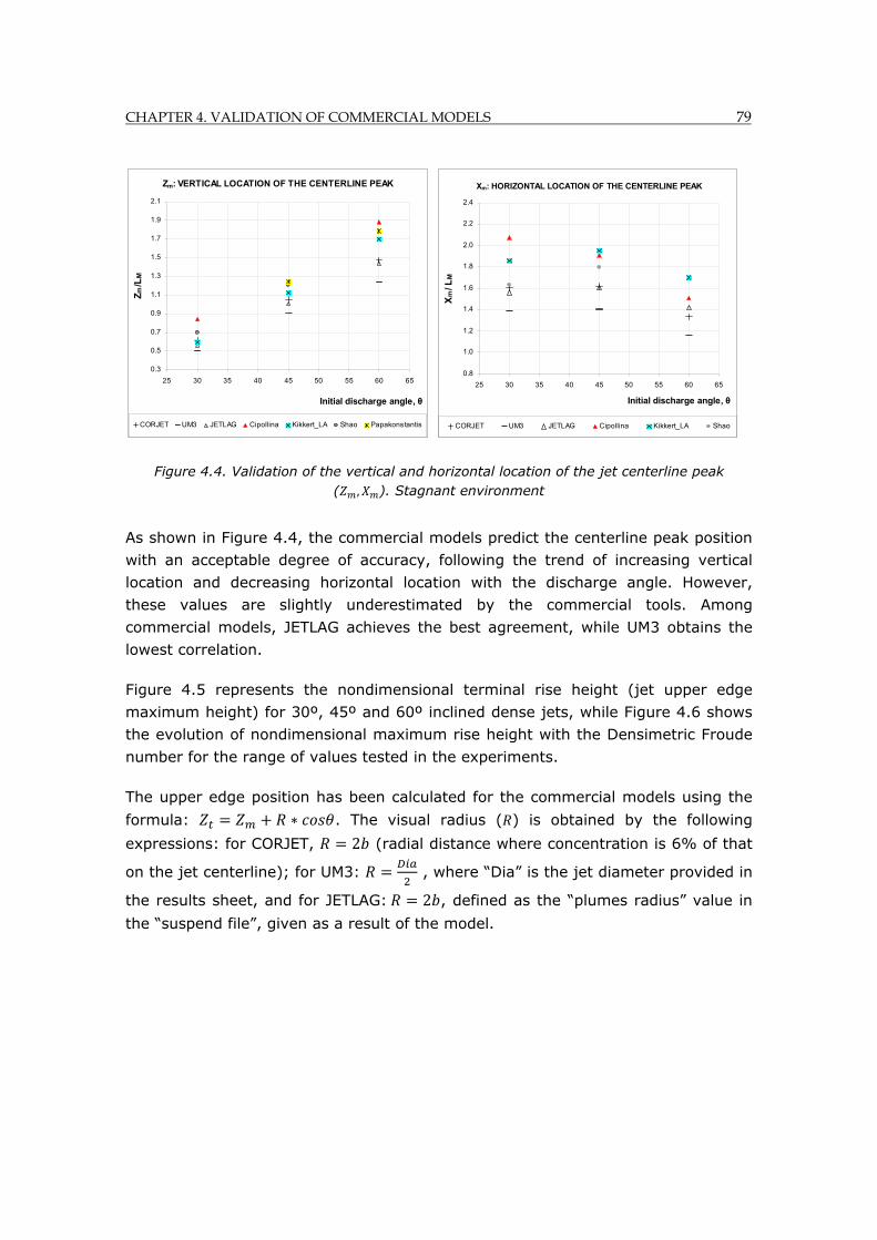
CHAPTER 4. VALIDATION OF COMMERCIAL MODELS 79
Figure 4.4. Validation of the vertical and horizontal location of the jet centerline peak ( , ). Stagnant environment
As shown in Figure 4.4, the commercial models predict the centerline peak position
with an acceptable degree of accuracy, following the trend of increasing vertical
location and decreasing horizontal location with the discharge angle. However,
these values are slightly underestimated by the commercial tools. Among
commercial models, JETLAG achieves the best agreement, while UM3 obtains the
lowest correlation.
Figure 4.5 represents the nondimensional terminal rise height (jet upper edge
maximum height) for 30º, 45º and 60º inclined dense jets, while Figure 4.6 shows
the evolution of nondimensional maximum rise height with the Densimetric Froude
number for the range of values tested in the experiments.
The upper edge position has been calculated for the commercial models using the
formula: . The visual radius ( ) is obtained by the following
expressions: for CORJET, 2 (radial distance where concentration is 6% of that
on the jet centerline); for UM3: , where “Dia” is the jet diameter provided in
the results sheet, and for JETLAG: 2 , defined as the “plumes radius” value in
the “suspend file”, given as a result of the model.
Zm: VERTICAL LOCATION OF THE CENTERLINE PEAK
0.3
0.5
0.7
0.9
1.1
1.3
1.5
1.7
1.9
2.1
25 30 35 40 45 50 55 60 65
Initial discharge angle, θ
Zm
/LM
CORJET UM3 JETLAG Cipollina Kikkert_LA Shao Papakonstantis
Xm: HORIZONTAL LOCATION OF THE CENTERLINE PEAK
0.8
1.0
1.2
1.4
1.6
1.8
2.0
2.2
2.4
25 30 35 40 45 50 55 60 65
Initial discharge angle, θ
Xm
/ LM
CORJET UM3 JETLAG Cipollina Kikkert_LA Shao
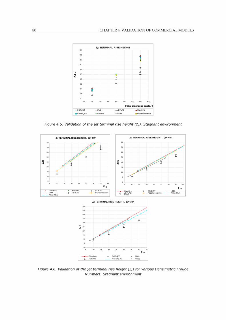
80 CHAPTER 4. VALIDATION OF COMMERCIAL MODELS
Figure 4.5. Validation of the jet terminal rise height ( ). Stagnant environment
Figure 4.6. Validation of the jet terminal rise height ( ) for various Densimetric Froude Numbers. Stagnant environment
Zt: TERMINAL RISE HEIGHT
0.7
0.9
1.1
1.3
1.5
1.7
1.9
2.1
2.3
2.5
2.7
25 30 35 40 45 50 55 60 65
Initial discharge angle, θ
Zt/L
M
CORJET UM3 JETLAG Cipollina
Kikkert_LA Roberts Shao Papakonstantis
Zt: TERMINAL RISE HEIGHT. (θ= 60º)
0
10
20
30
40
50
60
70
80
5 10 15 20 25 30 35 40 45
Frd
Z t/D
Cipollina Roberts CORJETUM3 JETLAG PapakonstantisKikkert(LA)
Zt: TERMINAL RISE HEIGHT. (θ= 45º)
0
10
20
30
40
50
60
70
80
5 10 15 20 25 30 35 40 45
Frd
Z t/ D
Cipollina CORJET UM3JETLAG Papakonstantis Kikkert(LA)Shao
Zt: TERMINAL RISE HEIGHT. (θ= 30º)
0
5
10
15
20
25
30
35
40
45
50
5 10 15 20 25 30 35 40 45
Frd
Z t/ D
Cipollina CORJET UM3
JETLAG Kikkert(LA) Shao
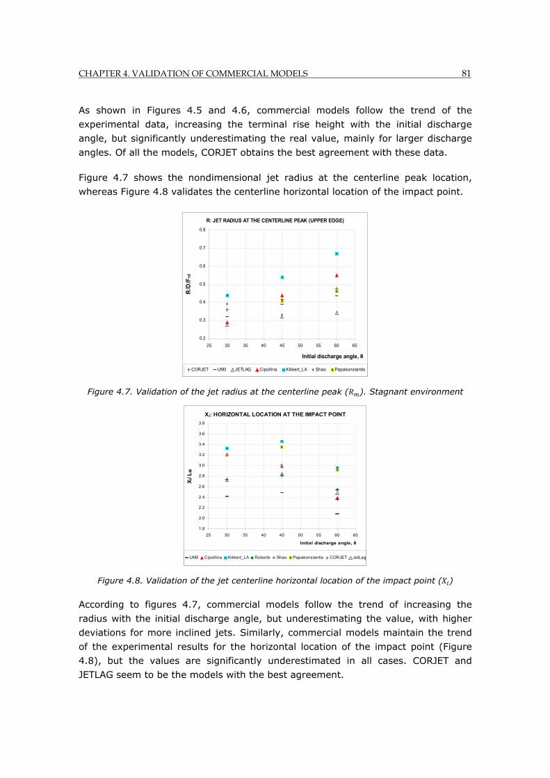
CHAPTER 4. VALIDATION OF COMMERCIAL MODELS 81
As shown in Figures 4.5 and 4.6, commercial models follow the trend of the
experimental data, increasing the terminal rise height with the initial discharge
angle, but significantly underestimating the real value, mainly for larger discharge
angles. Of all the models, CORJET obtains the best agreement with these data.
Figure 4.7 shows the nondimensional jet radius at the centerline peak location,
whereas Figure 4.8 validates the centerline horizontal location of the impact point.
Figure 4.7. Validation of the jet radius at the centerline peak ( ). Stagnant environment
Figure 4.8. Validation of the jet centerline horizontal location of the impact point ( )
According to figures 4.7, commercial models follow the trend of increasing the
radius with the initial discharge angle, but underestimating the value, with higher
deviations for more inclined jets. Similarly, commercial models maintain the trend
of the experimental results for the horizontal location of the impact point (Figure
4.8), but the values are significantly underestimated in all cases. CORJET and
JETLAG seem to be the models with the best agreement.
R: JET RADIUS AT THE CENTERLINE PEAK (UPPER EDGE)
0.2
0.3
0.4
0.5
0.6
0.7
0.8
25 30 35 40 45 50 55 60 65
Initial discharge angle, θ
R/D
/Frd
CORJET UM3 JETLAG Cipollina Kikkert_LA Shao Papakonstantis
Xi: HORIZONTAL LOCATION AT THE IMPACT POINT
1.8
2.0
2.2
2.4
2.6
2.8
3.0
3.2
3.4
3.6
3.8
25 30 35 40 45 50 55 60 65
Initial discharge angle, θ
Xi/
LM
UM3 Cipollina Kikkert_LA Roberts Shao Papakonstantis CORJET JetLag
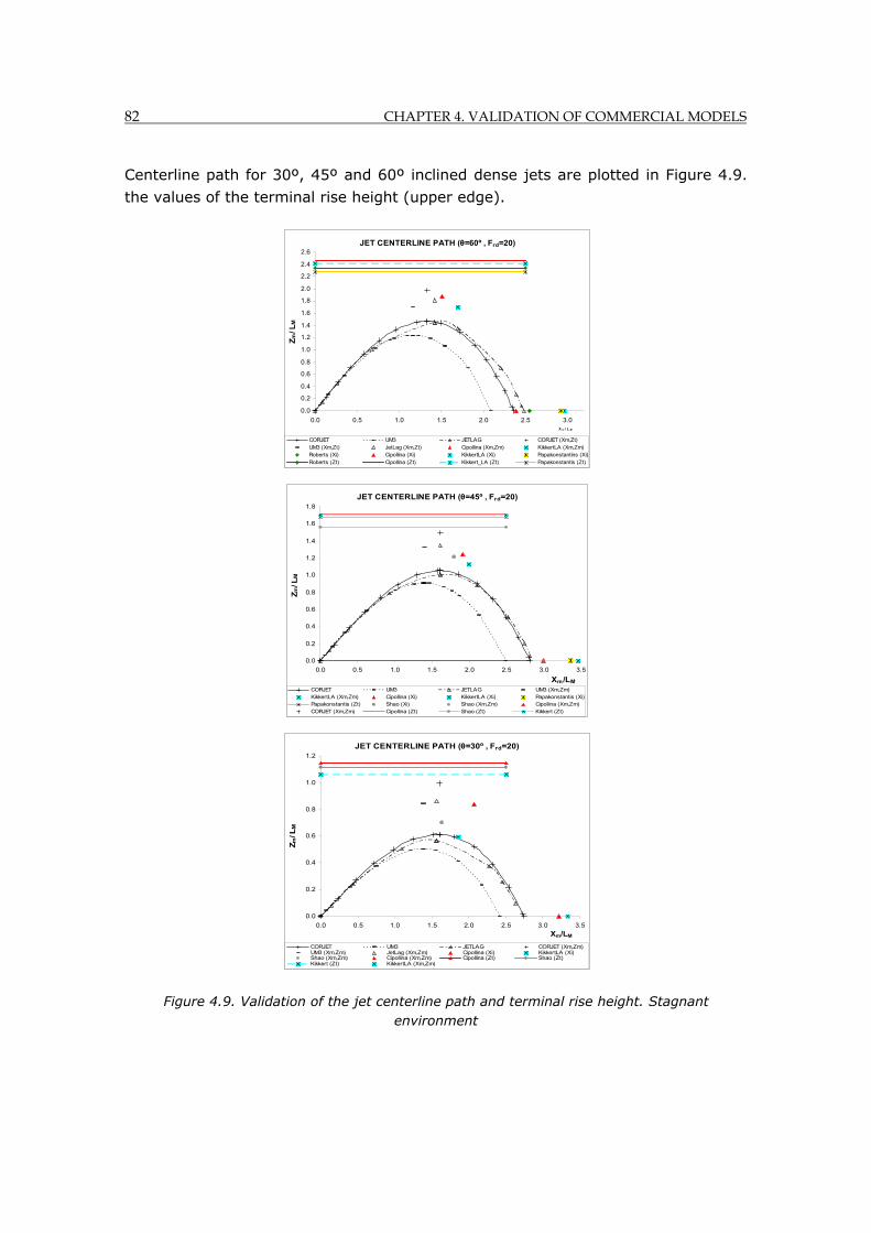
82 CHAPTER 4. VALIDATION OF COMMERCIAL MODELS
Centerline path for 30º, 45º and 60º inclined dense jets are plotted in Figure 4.9.
the values of the terminal rise height (upper edge).
Figure 4.9. Validation of the jet centerline path and terminal rise height. Stagnant environment
JET CENTERLINE PATH (θ=60º , Frd=20)
0.0
0.2
0.4
0.6
0.8
1.0
1.2
1.4
1.6
1.8
2.0
2.2
2.4
2.6
0.0 0.5 1.0 1.5 2.0 2.5 3.0X m / L M
Z m/ L
M
CORJET UM3 JETLAG CORJET (Xm,Zt)UM3 (Xm,Zt) JetLag (Xm,Zt) Cipollina (Xm,Zm) KikkertLA (Xm,Zm)Roberts (Xi) Cipollina (Xi) KikkertLA (Xi) Papakonstantins (Xi)Roberts (Zt) Cipollina (Zt) Kikkert_LA (Zt) Papakonstantis (Zt)
JET CENTERLINE PATH (θ=45º , Frd=20)
0.0
0.2
0.4
0.6
0.8
1.0
1.2
1.4
1.6
1.8
0.0 0.5 1.0 1.5 2.0 2.5 3.0 3.5
Xm/LM
Zm
/ LM
CORJET UM3 JETLAG UM3 (Xm,Zm)KikkertLA (Xm,Zm) Cipollina (Xi) KikkertLA (Xi) Papakonstantis (Xi)Papakonstantis (Zt) Shao (Xi) Shao (Xm,Zm) Cipollina (Xm,Zm)CORJET (Xm,Zm) Cipollina (Zt) Shao (Zt) Kikkert (Zt)
JET CENTERLINE PATH (θ=30º , Frd=20)
0.0
0.2
0.4
0.6
0.8
1.0
1.2
0.0 0.5 1.0 1.5 2.0 2.5 3.0 3.5
Xm/LM
Zm
/ LM
CORJET UM3 JETLAG CORJET (Xm,Zm)UM3 (Xm,Zm) JetLag (Xm,Zm) Cipollina (Xi) KikkertLA (Xi)Shao (Xm,Zm) Cipollina (Xm,Zm) Cipollina (Zt) Shao (Zt)Kikkert (Zt) KikkertLA (Xm,Zm)
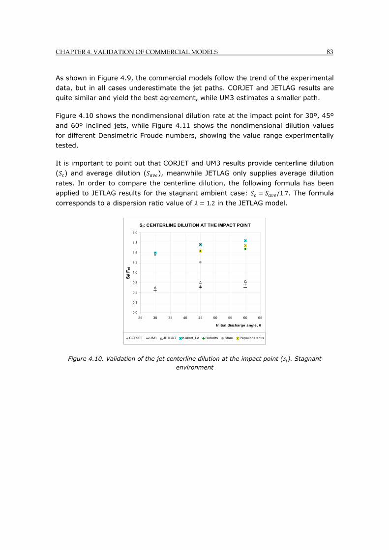
CHAPTER 4. VALIDATION OF COMMERCIAL MODELS 83
As shown in Figure 4.9, the commercial models follow the trend of the experimental
data, but in all cases underestimate the jet paths. CORJET and JETLAG results are
quite similar and yield the best agreement, while UM3 estimates a smaller path.
Figure 4.10 shows the nondimensional dilution rate at the impact point for 30º, 45º
and 60º inclined jets, while Figure 4.11 shows the nondimensional dilution values
for different Densimetric Froude numbers, showing the value range experimentally
tested.
It is important to point out that CORJET and UM3 results provide centerline dilution
( ) and average dilution ( ), meanwhile JETLAG only supplies average dilution
rates. In order to compare the centerline dilution, the following formula has been
applied to JETLAG results for the stagnant ambient case: /1.7. The formula
corresponds to a dispersion ratio value of 1.2 in the JETLAG model.
Figure 4.10. Validation of the jet centerline dilution at the impact point ( ). Stagnant environment
Si: CENTERLINE DILUTION AT THE IMPACT POINT
0.0
0.3
0.5
0.8
1.0
1.3
1.5
1.8
2.0
25 30 35 40 45 50 55 60 65
Initial discharge angle, θ
Si/
Frd
CORJET UM3 JETLAG Kikkert_LA Roberts Shao Papakonstantis
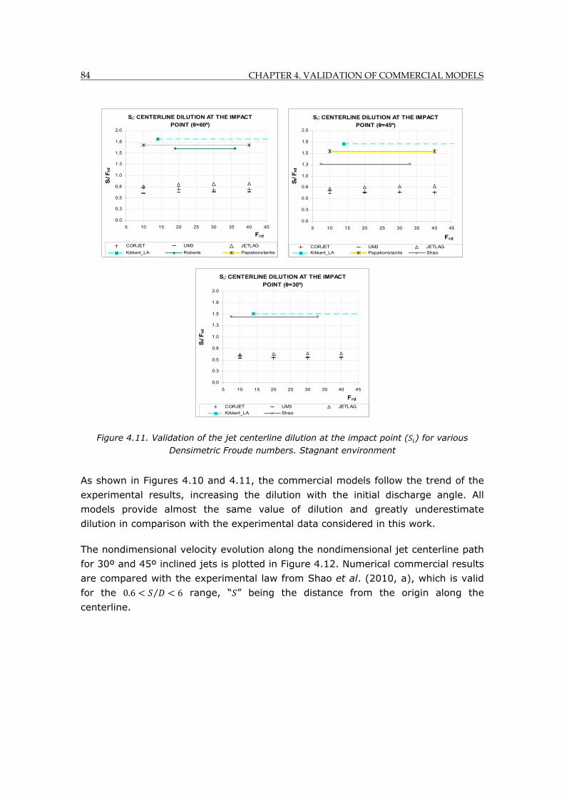
84 CHAPTER 4. VALIDATION OF COMMERCIAL MODELS
Figure 4.11. Validation of the jet centerline dilution at the impact point ( ) for various Densimetric Froude numbers. Stagnant environment
As shown in Figures 4.10 and 4.11, the commercial models follow the trend of the
experimental results, increasing the dilution with the initial discharge angle. All
models provide almost the same value of dilution and greatly underestimate
dilution in comparison with the experimental data considered in this work.
The nondimensional velocity evolution along the nondimensional jet centerline path
for 30º and 45º inclined jets is plotted in Figure 4.12. Numerical commercial results
are compared with the experimental law from Shao et al. (2010, a), which is valid
for the 0.6 ⁄ 6 range, “ ” being the distance from the origin along the
centerline.
Si: CENTERLINE DILUTION AT THE IMPACT
POINT (θ=60º)
0.0
0.3
0.5
0.8
1.0
1.3
1.5
1.8
2.0
5 10 15 20 25 30 35 40 45
Frd
Si/
Frd
CORJET UM3 JETLAG
Kikkert_LA Roberts Papakonstantis
Si: CENTERLINE DILUTION AT THE IMPACT
POINT (θ=45º)
0.0
0.3
0.5
0.8
1.0
1.3
1.5
1.8
2.0
5 10 15 20 25 30 35 40 45
Frd
Si/
Frd
CORJET UM3 JETLAGKikkert_LA Papakonstantis Shao
Si: CENTERLINE DILUTION AT THE IMPACT
POINT (θ=30º)
0.0
0.3
0.5
0.8
1.0
1.3
1.5
1.8
2.0
5 10 15 20 25 30 35 40 45
Frd
Si/
Frd
CORJET UM3 JETLAG
Kikkert_LA Shao
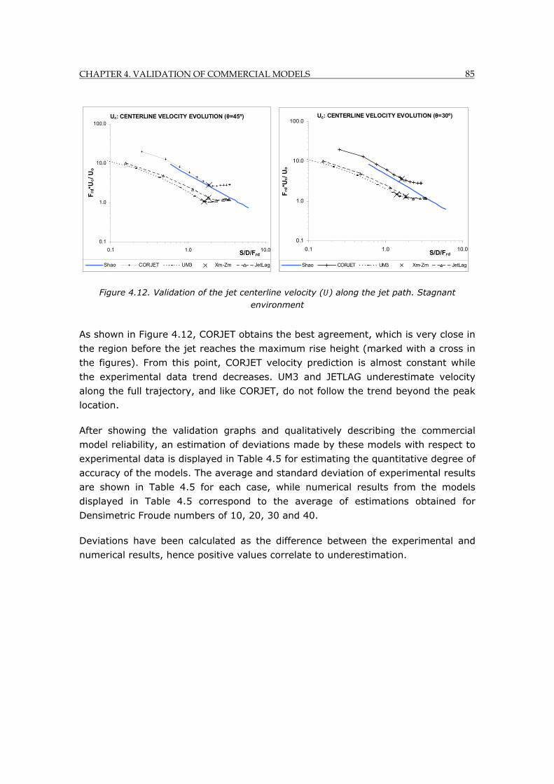
CHAPTER 4. VALIDATION OF COMMERCIAL MODELS 85
Figure 4.12. Validation of the jet centerline velocity ( ) along the jet path. Stagnant environment
As shown in Figure 4.12, CORJET obtains the best agreement, which is very close in
the region before the jet reaches the maximum rise height (marked with a cross in
the figures). From this point, CORJET velocity prediction is almost constant while
the experimental data trend decreases. UM3 and JETLAG underestimate velocity
along the full trajectory, and like CORJET, do not follow the trend beyond the peak
location.
After showing the validation graphs and qualitatively describing the commercial
model reliability, an estimation of deviations made by these models with respect to
experimental data is displayed in Table 4.5 for estimating the quantitative degree of
accuracy of the models. The average and standard deviation of experimental results
are shown in Table 4.5 for each case, while numerical results from the models
displayed in Table 4.5 correspond to the average of estimations obtained for
Densimetric Froude numbers of 10, 20, 30 and 40.
Deviations have been calculated as the difference between the experimental and
numerical results, hence positive values correlate to underestimation.
Uc: CENTERLINE VELOCITY EVOLUTION (θ=45º)
0.1
1.0
10.0
100.0
0.1 1.0 10.0S/D/Frd
Frd
*Uc/ U
o
Shao CORJET UM3 Xm-Zm JetLag
Uc: CENTERLINE VELOCITY EVOLUTION (θ=30º)
0.1
1.0
10.0
100.0
0.1 1.0 10.0S/D/Frd
Frd
*Uc/
Uo
Shao CORJET UM3 Xm-Zm JetLag
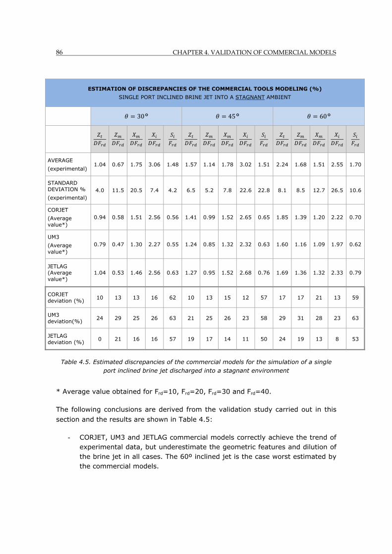
86 CHAPTER 4. VALIDATION OF COMMERCIAL MODELS
Table 4.5. Estimated discrepancies of the commercial models for the simulation of a single port inclined brine jet discharged into a stagnant environment
* Average value obtained for Frd=10, Frd=20, Frd=30 and Frd=40.
The following conclusions are derived from the validation study carried out in this
section and the results are shown in Table 4.5:
- CORJET, UM3 and JETLAG commercial models correctly achieve the trend of experimental data, but underestimate the geometric features and dilution of the brine jet in all cases. The 60º inclined jet is the case worst estimated by the commercial models.
ESTIMATION OF DISCREPANCIES OF THE COMMERCIAL TOOLS MODELING (%)
SINGLE PORT INCLINED BRINE JET INTO A STAGNANT AMBIENT
30° 45° 60°
AVERAGE
(experimental) 1.04 0.67 1.75 3.06 1.48 1.57 1.14 1.78 3.02 1.51 2.24 1.68 1.51 2.55 1.70
STANDARD DEVIATION %
(experimental) 4.0 11.5 20.5 7.4 4.2 6.5 5.2 7.8 22.6 22.8 8.1 8.5 12.7 26.5 10.6
CORJET
(Average value*)
0.94 0.58 1.51 2.56 0.56 1.41 0.99 1.52 2.65 0.65 1.85 1.39 1.20 2.22 0.70
UM3
(Average value*)
0.79 0.47 1.30 2.27 0.55 1.24 0.85 1.32 2.32 0.63 1.60 1.16 1.09 1.97 0.62
JETLAG (Average value*)
1.04 0.53 1.46 2.56 0.63 1.27 0.95 1.52 2.68 0.76 1.69 1.36 1.32 2.33 0.79
CORJET deviation (%)
10 13 13 16 62 10 13 15 12 57 17 17 21 13 59
UM3 deviation(%)
24 29 25 26 63 21 25 26 23 58 29 31 28 23 63
JETLAG deviation (%)
0 21 16 16 57 19 17 14 11 50 24 19 13 8 53
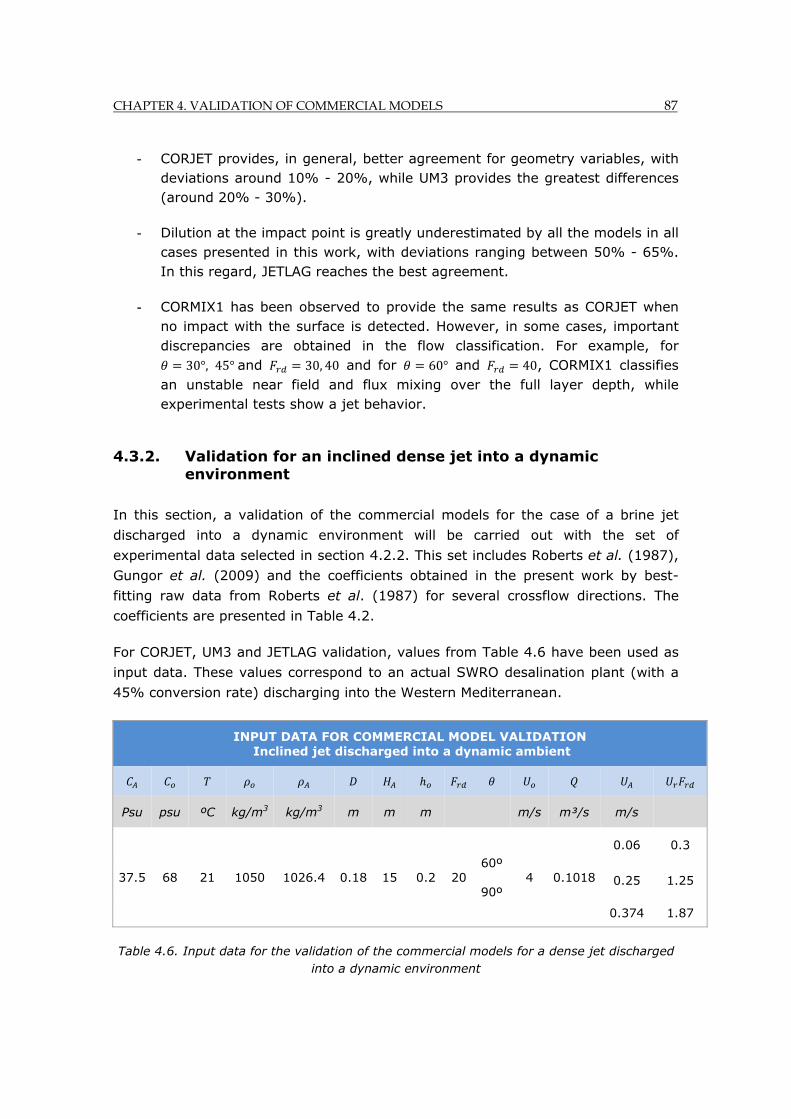
CHAPTER 4. VALIDATION OF COMMERCIAL MODELS 87
- CORJET provides, in general, better agreement for geometry variables, with deviations around 10% - 20%, while UM3 provides the greatest differences (around 20% - 30%).
- Dilution at the impact point is greatly underestimated by all the models in all cases presented in this work, with deviations ranging between 50% - 65%. In this regard, JETLAG reaches the best agreement.
- CORMIX1 has been observed to provide the same results as CORJET when no impact with the surface is detected. However, in some cases, important discrepancies are obtained in the flow classification. For example, for
30°, 45° and 30, 40 and for 60° and 40, CORMIX1 classifies an unstable near field and flux mixing over the full layer depth, while experimental tests show a jet behavior.
4.3.2. Validation for an inclined dense jet into a dynamic environment
In this section, a validation of the commercial models for the case of a brine jet
discharged into a dynamic environment will be carried out with the set of
experimental data selected in section 4.2.2. This set includes Roberts et al. (1987),
Gungor et al. (2009) and the coefficients obtained in the present work by best-
fitting raw data from Roberts et al. (1987) for several crossflow directions. The
coefficients are presented in Table 4.2.
For CORJET, UM3 and JETLAG validation, values from Table 4.6 have been used as
input data. These values correspond to an actual SWRO desalination plant (with a
45% conversion rate) discharging into the Western Mediterranean.
INPUT DATA FOR COMMERCIAL MODEL VALIDATION Inclined jet discharged into a dynamic ambient
Psu psu ºC kg/m3 kg/m3 m m m m/s m³/s m/s
37.5 68 21 1050 1026.4 0.18 15 0.2 20 60º
90º
4 0.1018
0.06 0.3
0.25 1.25
0.374 1.87
Table 4.6. Input data for the validation of the commercial models for a dense jet discharged into a dynamic environment

88 CHAPTER 4. VALIDATION OF COMMERCIAL MODELS
For the input data shown in Table 4.6 and the crossflow directions ( 180°, 150°,
120°, 90°, 60°, 30°, 0°), CORJET, UM3 and JETLAG models have been run to obtain
the numerical estimation of the variables of interest: , , and and these
values have been compared with experimental values shown in Table 4.2.
Figures 4.13 to 4.16 show some of the validation graphs for the previous variables.
The vertical axis represents the nondimensional magnitudes, while the horizontal
axis represents values. variable refers to the ambient velocity ( ) relative
to the jet discharge velocity ( ), ⁄ . Each figure corresponds to a
different value combination of the initial discharge angle with respect to the bottom
( ) and angle of crossflow relative to the horizontal plane containing the jet axis ( )
or relative to the vertical plane containing the nozzle axis ( ), being 90°.
Commercial model results are represented by the same symbols used for the
stagnant ambient validation (crosses for CORJET; lines for UM3 and triangles for
JETLAG results). Roberts et al. (1987) and Gungor et al. (2009) formula results are
represented by a dotted line. Results obtained from the formulas calculated in the
present work by best-fitting raw data from Roberts et al. (1987) are highlighted by
a solid line. A qualitative description of the validation is included below each figure.
Figure 4.13 shows the validation for the terminal rise height ( ) for different
values.
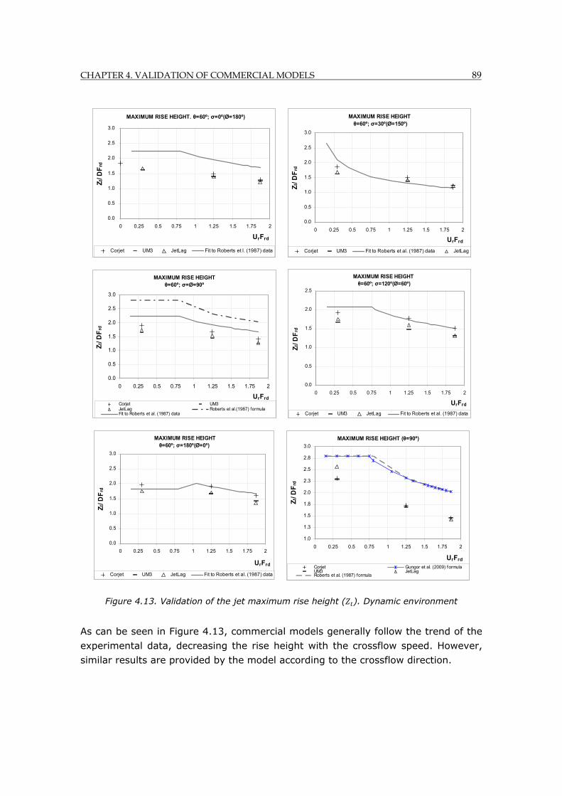
CHAPTER 4. VALIDATION OF COMMERCIAL MODELS 89
Figure 4.13. Validation of the jet maximum rise height ( ). Dynamic environment
As can be seen in Figure 4.13, commercial models generally follow the trend of the
experimental data, decreasing the rise height with the crossflow speed. However,
similar results are provided by the model according to the crossflow direction.
MAXIMUM RISE HEIGHT. θ=60º; σ=0º(Ø=180º)
0.0
0.5
1.0
1.5
2.0
2.5
3.0
0 0.25 0.5 0.75 1 1.25 1.5 1.75 2
UrFrd
Zt/
DF
rd
Corjet UM3 JetLag Fit to Roberts et l. (1987) data
MAXIMUM RISE HEIGHT θ=60º; σ=30º(Ø=150º)
0.0
0.5
1.0
1.5
2.0
2.5
3.0
0 0.25 0.5 0.75 1 1.25 1.5 1.75 2
UrFrd
Zt/
DF
rd
Corjet UM3 Fit to Roberts et al. (1987) data JetLag
MAXIMUM RISE HEIGHT θ=60º; σ=Ø=90º
0.0
0.5
1.0
1.5
2.0
2.5
3.0
0 0.25 0.5 0.75 1 1.25 1.5 1.75 2
UrFrd
Zt/
DF
rd
Corjet UM3JetLag Roberts et al.(1987) formulaFit to Roberts et al. (1987) data
MAXIMUM RISE HEIGHT θ=60º; σ=120º(Ø=60º)
0.0
0.5
1.0
1.5
2.0
2.5
0 0.25 0.5 0.75 1 1.25 1.5 1.75 2
UrFrd
Zt/
DF
rd
Corjet UM3 JetLag Fit to Roberts et al. (1987) data
MAXIMUM RISE HEIGHT θ=60º; σ=180º(Ø=0º)
0.0
0.5
1.0
1.5
2.0
2.5
3.0
0 0.25 0.5 0.75 1 1.25 1.5 1.75 2
UrFrd
Zt/
DF
rd
Corjet UM3 JetLag Fit to Roberts et al. (1987) data
MAXIMUM RISE HEIGHT (θ=90º)
1.0
1.3
1.5
1.8
2.0
2.3
2.5
2.8
3.0
0 0.25 0.5 0.75 1 1.25 1.5 1.75 2
UrFrd
Zt/
DF
rd
Corjet Gungor et al. (2009) formulaUM3 JetLagRoberts et al. (1987) formula
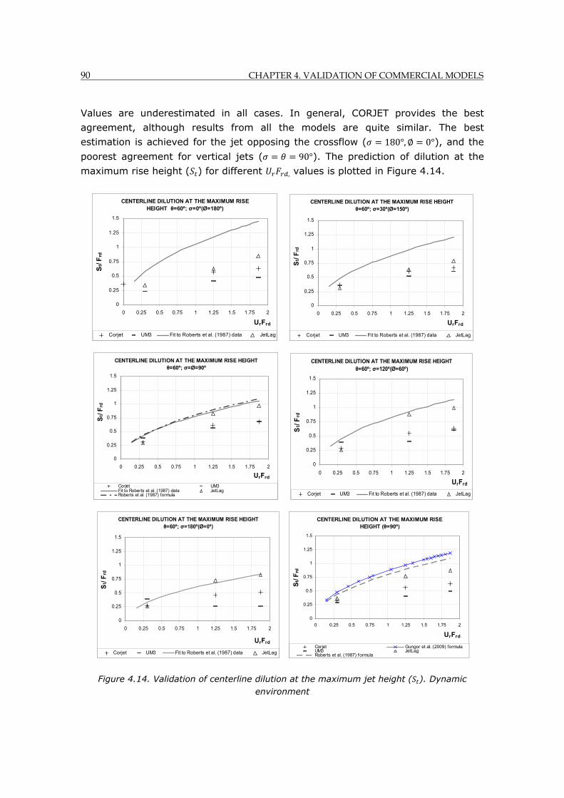
90 CHAPTER 4. VALIDATION OF COMMERCIAL MODELS
Values are underestimated in all cases. In general, CORJET provides the best
agreement, although results from all the models are quite similar. The best
estimation is achieved for the jet opposing the crossflow ( 180°, 0°), and the
poorest agreement for vertical jets ( 90°). The prediction of dilution at the
maximum rise height ( ) for different , values is plotted in Figure 4.14.
Figure 4.14. Validation of centerline dilution at the maximum jet height ( ). Dynamic environment
CENTERLINE DILUTION AT THE MAXIMUM RISE HEIGHT θ=60º; σ=0º(Ø=180º)
0
0.25
0.5
0.75
1
1.25
1.5
0 0.25 0.5 0.75 1 1.25 1.5 1.75 2
UrFrd
St/
Frd
Corjet UM3 Fit to Roberts et al. (1987) data JetLag
CENTERLINE DILUTION AT THE MAXIMUM RISE HEIGHT θ=60º; σ=30º(Ø=150º)
0
0.25
0.5
0.75
1
1.25
1.5
0 0.25 0.5 0.75 1 1.25 1.5 1.75 2
UrFrd
St/
Frd
Corjet UM3 Fit to Roberts et al. (1987) data JetLag
CENTERLINE DILUTION AT THE MAXIMUM RISE HEIGHT θ=60º; σ=Ø=90º
0
0.25
0.5
0.75
1
1.25
1.5
0 0.25 0.5 0.75 1 1.25 1.5 1.75 2
UrFrd
St/
Frd
Corjet UM3Fit to Roberts et al. (1987) data JetLagRoberts et al. (1987) formula
CENTERLINE DILUTION AT THE MAXIMUM RISE HEIGHT θ=60º; σ=120º(Ø=60º)
0
0.25
0.5
0.75
1
1.25
1.5
0 0.25 0.5 0.75 1 1.25 1.5 1.75 2
UrFrd
St/
Frd
Corjet UM3 Fit to Roberts et al. (1987) data JetLag
CENTERLINE DILUTION AT THE MAXIMUM RISE HEIGHT θ=60º; σ=180º(Ø=0º)
0
0.25
0.5
0.75
1
1.25
1.5
0 0.25 0.5 0.75 1 1.25 1.5 1.75 2
UrFrd
St/
Frd
Corjet UM3 Fit to Roberts et al. (1987) data JetLag
CENTERLINE DILUTION AT THE MAXIMUM RISE HEIGHT (θ=90º)
0
0.25
0.5
0.75
1
1.25
1.5
0 0.25 0.5 0.75 1 1.25 1.5 1.75 2
UrFrd
St/
Frd
Corjet Gungor et al. (2009) formulaUM3 JetLagRoberts et al. (1987) formula
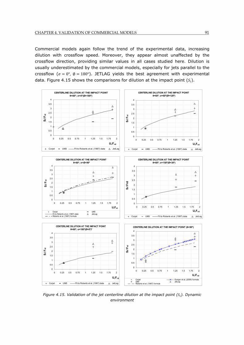
CHAPTER 4. VALIDATION OF COMMERCIAL MODELS 91
Commercial models again follow the trend of the experimental data, increasing
dilution with crossflow speed. Moreover, they appear almost unaffected by the
crossflow direction, providing similar values in all cases studied here. Dilution is
usually underestimated by the commercial models, especially for jets parallel to the
crossflow ( 0°, 180°). JETLAG yields the best agreement with experimental
data. Figure 4.15 shows the comparisons for dilution at the impact point ( ).
Figure 4.15. Validation of the jet centerline dilution at the impact point ( ). Dynamic environment
CENTERLINE DILUTION AT THE IMPACT POINT θ=60º; σ=0º(Ø=180º)
0
0.5
1
1.5
2
2.5
3
3.5
4
0 0.25 0.5 0.75 1 1.25 1.5 1.75 2
UrFrd
Si/
Frd
Corjet UM3 Fit to Roberts et al. (1987) data JetLag
CENTERLINE DILUTION AT THE IMPACT POINT θ=60º; σ=60º(Ø=120º)
0
0.5
1
1.5
2
2.5
3
3.5
4
0 0.25 0.5 0.75 1 1.25 1.5 1.75 2
UrFrd
Si/
Frd
Corjet UM3 Fit to Roberts et al. (1987) data JetLag
CENTERLINE DILUTION AT THE IMPACT POINT θ=60º; σ=Ø=90º
0
0.5
1
1.5
2
2.5
3
3.5
4
0 0.25 0.5 0.75 1 1.25 1.5 1.75 2
UrFrd
Si/
Frd
Corjet UM3Fit to Roberts et al. (1987) data JetLagRoberts et al. (1987) formula
CENTERLINE DILUTION AT THE IMPACT POINT θ=60º; σ=150º(Ø=30º)
0
0.5
1
1.5
2
2.5
3
3.5
4
0 0.25 0.5 0.75 1 1.25 1.5 1.75 2
UrFrd
Si/
Frd
Corjet UM3 Fit to Roberts et al. (1987) data JetLag
CENTERLINE DILUTION AT THE IMPACT POINT θ=60º; σ=180º(Ø=0º)º
0
0.5
1
1.5
2
2.5
3
3.5
4
0 0.25 0.5 0.75 1 1.25 1.5 1.75 2
UrFrd
Si/
Frd
Corjet UM3 Fit to Roberts et al. (1987) data JetLag
CENTERLINE DILUTION AT THE IMPACT POINT (θ=90º)
0
0.5
1
1.5
2
2.5
3
3.5
4
0 0.25 0.5 0.75 1 1.25 1.5 1.75 2
UrFrd
Si/
Frd
Corjet Gungor et al. (2009) formulaUM3 JetLagRoberts et al. (1987) formula
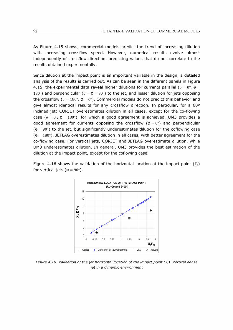
92 CHAPTER 4. VALIDATION OF COMMERCIAL MODELS
As Figure 4.15 shows, commercial models predict the trend of increasing dilution
with increasing crossflow speed. However, numerical results evolve almost
independently of crossflow direction, predicting values that do not correlate to the
results obtained experimentally.
Since dilution at the impact point is an important variable in the design, a detailed
analysis of the results is carried out. As can be seen in the different panels in Figure
4.15, the experimental data reveal higher dilutions for currents parallel ( 0°,
180°) and perpendicular ( 90°) to the jet, and lesser dilution for jets opposing
the crossflow ( 180°, 0°). Commercial models do not predict this behavior and
give almost identical results for any crossflow direction. In particular, for a 60º
inclined jet: CORJET overestimates dilution in all cases, except for the co-flowing
case ( 0°, 180°), for which a good agreement is achieved. UM3 provides a
good agreement for currents opposing the crossflow ( 0°) and perpendicular
( 90°) to the jet, but significantly underestimates dilution for the coflowing case
( 180°). JETLAG overestimates dilution in all cases, with better agreement for the
co-flowing case. For vertical jets, CORJET and JETLAG overestimate dilution, while
UM3 underestimates dilution. In general, UM3 provides the best estimation of the
dilution at the impact point, except for the coflowing case.
Figure 4.16 shows the validation of the horizontal location at the impact point ( )
for vertical jets ( 90°).
Figure 4.16. Validation of the jet horizontal location of the impact point ( ). Vertical dense jet in a dynamic environment
HORIZONTAL LOCATION OF THE IMPACT POINT (Frd=20 and θ=90º)
0
2
4
6
8
10
12
0 0.25 0.5 0.75 1 1.25 1.5 1.75 2
UrFrd
Xi/
DF
rd
Corjet Gungor et al. (2009) formula UM3 JetLag

CHAPTER 4. VALIDATION OF COMMERCIAL MODELS 93
As shown in Figure 4.16, commercial models are able to predict the trend observed
in the experiments, increasing the distance with the crossflow speed, but this
magnitude is significantly underestimated.
As a summary of the validations, an estimation of deviations of numerical results
with respect to the experimental data is shown in Table 4.7 and Table 4.8, for the
cases: 0.3, 1.25 and 1.87. Deviations, shown as percentage values, have
been calculated as the difference between the experimental and the numerical
results, hence positive values mean underestimation.
Table 4.7. Estimated deviations for a single-port dense jet discharged into a dynamic environment. Coflowing and counterflowing cases
ESTIMATION OF DEVIATIONS OF MODELING RESULTS (%) SINGLE PORT BRINE DENSE JET INTO A DYNAMIC ENVIRONMENT
Discrepancies of the commercial models with respect to the
formulas obtained by best fitting raw data from Roberts et al.
(1987)
Case: 60°, 180° Coflowing: jet parallel to
crossflow
Discrepancies of the commercial models with respect to the
formulas obtained by best fitting raw data from Roberts et al.
(1987).
Case: 60°, 0° Counterflowing: jet opposing
crossflow
MODELS
values
Variables Variables
CORJET
0.30 38 15 18 18 2 -9
1.25 52 -6 24 33 -63 -1
1.87 56 -1 24 39 -56 4
UM3
0.30 61 40 28 -16 10 5
1.25 65 34 28 62 21 13
1.87 68 34 26 69 -6 15
JETLAG
0.30 41 27 26 23 3 4
1.25 47 -15 28 -7 -86 11
1.87 41 -15 28 2 -70 19
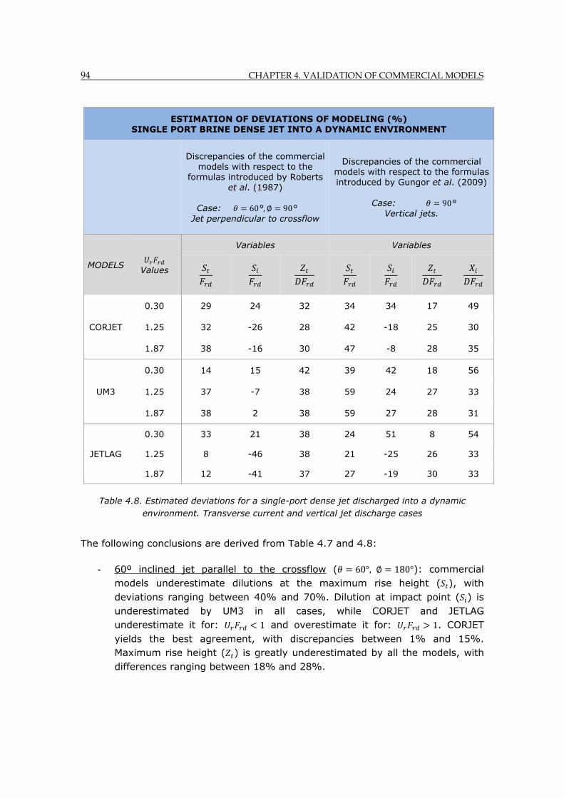
94 CHAPTER 4. VALIDATION OF COMMERCIAL MODELS
Table 4.8. Estimated deviations for a single-port dense jet discharged into a dynamic environment. Transverse current and vertical jet discharge cases
The following conclusions are derived from Table 4.7 and 4.8:
- 60º inclined jet parallel to the crossflow ( 60°, 180°): commercial models underestimate dilutions at the maximum rise height ( ), with deviations ranging between 40% and 70%. Dilution at impact point ( ) is underestimated by UM3 in all cases, while CORJET and JETLAG underestimate it for: 1 and overestimate it for: 1. CORJET yields the best agreement, with discrepancies between 1% and 15%. Maximum rise height ( ) is greatly underestimated by all the models, with differences ranging between 18% and 28%.
ESTIMATION OF DEVIATIONS OF MODELING (%) SINGLE PORT BRINE DENSE JET INTO A DYNAMIC ENVIRONMENT
Discrepancies of the commercial models with respect to the
formulas introduced by Roberts et al. (1987)
Case: 60°, 90°
Jet perpendicular to crossflow
Discrepancies of the commercial models with respect to the formulas introduced by Gungor et al. (2009)
Case: 90°
Vertical jets.
MODELS
Values
Variables Variables
CORJET
0.30 29 24 32 34 34 17 49
1.25 32 -26 28 42 -18 25 30
1.87 38 -16 30 47 -8 28 35
UM3
0.30 14 15 42 39 42 18 56
1.25 37 -7 38 59 24 27 33
1.87 38 2 38 59 27 28 31
JETLAG
0.30 33 21 38 24 51 8 54
1.25 8 -46 38 21 -25 26 33
1.87 12 -41 37 27 -19 30 33
CHAPTER 4. VALIDATION OF COMMERCIAL MODELS 95
- 60º inclined jet opposing the crossflow ( 60°, 0°): dilution at the impact point ( ) is significantly overestimated by CORJET (deviations around 60%) and also by JETLAG (deviations between 70% and 85%) for 1. UM3 provides the best estimation for this magnitude, with discrepancies between 5% and 20%. Terminal rise height ( ) is quite well predicted by all models, with a maximum deviation of 20%.
- 60º inclined jet perpendicular to the crossflow ( 60°, 90°): dilution at the impact point ( ) is overestimated and underestimated depending on the case and model. UM3 provides the best agreement for this magnitude (errors between 2% and 15%), while JETLAG and CORJET underestimate dilution for lower and overestimate it for higher (deviations between 25% and 50%). Maximum rise height ( ) is underestimated in all cases (deviations between 30% and 40%).
- Vertical jets ( 90°). Dilution at the maximum rise height ( ) is underestimated by the commercial models, with the best agreement given by JETLAG (discrepancies around 20% - 30%) and the poorest by UM3. Dilution at the impact point ( ) is underestimated by UM3 (deviations between 25% and 40%), while CORJET and JETLAG overestimate it for:
0.75. The best estimation of is provided by CORJET (differences between 10% and 30%). Maximum rise height ( ) is underestimated by all the commercial models (deviations between 30% and 50%). Horizontal location of the impact point ( ) is also underestimated (discrepancies between 30% and 60%).
4.4. Conclusions
This work focuses on the validation of commercial models used for brine discharge
modeling by comparing numerical results with experimental data available. A high
number of varied cases have been included (more than fifty cases of validation run
with the four models; in total more than 200 cases).
The following conclusions and recommendations can be drawn for the use of
commercial tools for modeling brine dense jets, based on comparisons with selected
experimental data:
- Regarding the reliability of commercial models: tools based on the integration of differential equations, such as CORJET, UM3 and JETLAG, are a good alternative for dense jet modeling in cases of unlimited environments. Regarding the CORMIX1 subsystem, based on the dimensional analysis, important errors have been detected in flux
96 CHAPTER 4. VALIDATION OF COMMERCIAL MODELS
classification in some cases, especially for high Densimetric Froude numbers (see Section 4.4.2).
- Regarding CORJET, UM3 and JETLAG degree of accuracy for dense jets discharged into a stagnant ambient, validation reveals that these models underestimate jet dimensions in all cases. Terminal rise height ( ) deviations are between 10% and 30% and increase with the initial discharge angle. CORJET yields the best agreement, with deviations around 10% - 17%. With respect to dilution at the impact point ( ), all models significantly underestimate the values, with deviations ranging between 50% and 65%. These commercial models are therefore very conservative when estimating the dilution rate.
- Regarding CORJET, UM3 and JETLAG degree of accuracy for dense jets discharged into a dynamic environment, validation reveals that these models, following the trend of the experimental data, increase dilution while decreasing maximum rise height when increasing current speed. Important discrepancies, nevertheless, are made by the commercial models when predicting the influence of crossflow direction on jet behavior, since they are almost insensitive to this parameter. Analyzing each variable:
o Maximum rise height ( ): for a 60º inclined jet, the experimental data of Gungor et al. (2009) obtained higher values for a jet opposing ( 0°) and perpendicular ( 90°) to the current, while the commercial models provide similar results regardless of crossflow direction. Terminal rise height ( ) is in general underestimated by the commercial models, especially for vertical jets and 60º inclined jets parallel to the crossflow ( 180°), (deviations between 30% and 40%).
o Dilution at the impact point ( ): for a 60º inclined jet, experimental data of Gungor et al. (2009) obtained the highest dilutions for a jet perpendicular ( 90°) and overall parallel ( 180°) to the crossflow, while the lowest values of are obtained for a jet opposing the crossflow ( 0°). CORJET and JETLAG models, however, provide almost the same value of dilution independent of crossflow direction, with slightly higher values for transverse currents ( 90°). UM3 better follows the trend of the experimental data and gives higher dilution for jets perpendicular ( 90°) to the crossflow, but dilution rates obtained for jets parallel and opposing are still quite similar. With respect to the errors: for the cases of an inclined jet parallel, opposing and perpendicular to the crossflow, the commercial
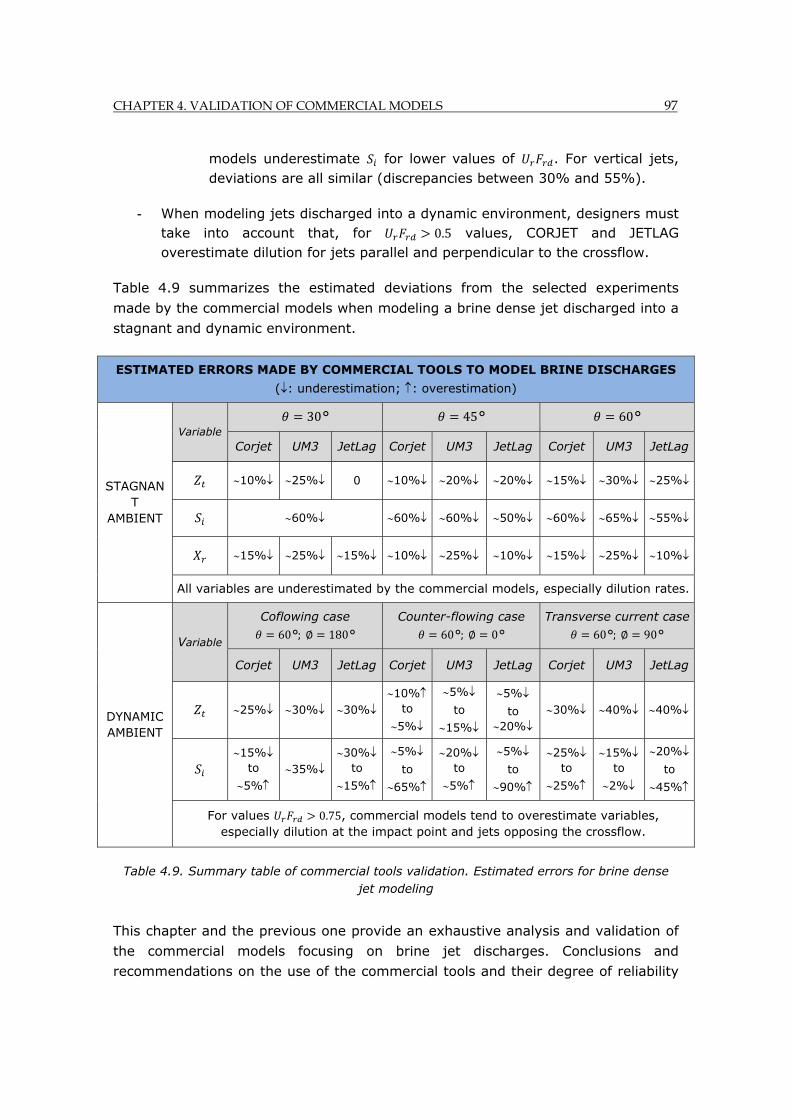
CHAPTER 4. VALIDATION OF COMMERCIAL MODELS 97
models underestimate for lower values of . For vertical jets, deviations are all similar (discrepancies between 30% and 55%).
- When modeling jets discharged into a dynamic environment, designers must take into account that, for 0.5 values, CORJET and JETLAG overestimate dilution for jets parallel and perpendicular to the crossflow.
Table 4.9 summarizes the estimated deviations from the selected experiments
made by the commercial models when modeling a brine dense jet discharged into a
stagnant and dynamic environment.
ESTIMATED ERRORS MADE BY COMMERCIAL TOOLS TO MODEL BRINE DISCHARGES
(: underestimation; : overestimation)
STAGNANT
AMBIENT
Variable 30° 45° 60°
Corjet UM3 JetLag Corjet UM3 JetLag Corjet UM3 JetLag
10% 25% 0 10% 20% 20% 15% 30% 25%
60% 60% 60% 50% 60% 65% 55%
15% 25% 15% 10% 25% 10% 15% 25% 10%
All variables are underestimated by the commercial models, especially dilution rates.
DYNAMIC AMBIENT
Variable
Coflowing case 60°; 180°
Counter-flowing case 60°; 0°
Transverse current case 60°; 90°
Corjet UM3 JetLag Corjet UM3 JetLag Corjet UM3 JetLag
25% 30% 30% 10%
to
5%
5%
to
15%
5%
to 20%
30% 40% 40%
15%
to
5% 35%
30% to
15%
5%
to
65%
20% to
5%
5%
to
90%
25% to
25%
15% to
2%
20%
to
45%
For values 0.75, commercial models tend to overestimate variables, especially dilution at the impact point and jets opposing the crossflow.
Table 4.9. Summary table of commercial tools validation. Estimated errors for brine dense jet modeling
This chapter and the previous one provide an exhaustive analysis and validation of
the commercial models focusing on brine jet discharges. Conclusions and
recommendations on the use of the commercial tools and their degree of reliability

98 CHAPTER 4. VALIDATION OF COMMERCIAL MODELS
aim to help developers, designers and environmental authorities in the discharge
design and environmental impact assessments of desalination projects.
According to the results, significant discrepancies have been found overall between
the commercial model results and the experimental data, in the estimation of
dilution rates. These discrepancies reveal the need for further review regarding the
simplified hypothesis and closure models assumed by commercial models. This
review is carried out in Chapters 5 and 6. Moreover, new alternative simulation
tools for brine discharges, calibrated with high quality experimental data, are also
required to ensure a high reliability in the prediction of brine discharge behavior.
The new tools developed in this Thesis, namely “BrIHne” tools, are presented in
Chapter 9.
CHAPTER 5. EXPERIMENTAL STUDY OF BRINE DISCHARGES 99
Chapter 5. EXPERIMENTAL STUDY OF BRINE JET DISCHARGES USING LASER ANEMOMETRY
Chapter 5 EXPERIMENTAL STUDY OF BRINE JET DISCHARGES USING LASER ANEMOMETRY
Summary
In the last two decades, experiments using non-intrusive optical techniques have
gained importance as an alternative to conventional measurements. However, at
the moment, there are few studies applying these techniques to the
characterization of brine discharges behavior. Moreover, those existing do not
provide detailed information regarding the experimental procedure and the flow
processes.
These gaps, together with the need for a high quality and large resolution
experimental database to calibrate and validate numerical models, justify the
carrying on of new experiments in IH Cantabria. PIV (Particle Image Velocimetry)
and PLIF (Planar Laser Induced Fluorescence) optical techniques have been used to
characterize the velocity and concentration flow fields, respectively.
Experiments focus on discharges through submerged and inclined jets and
homogeneous and stagnant environments. The whole near field region, including
the jet path and the spreading layer, has been experimentally characterized.
This chapter describes the setup and the procedure developed to apply these
techniques to the characterization of the near field region of brine jet discharges.
Moreover, the chapter explains the criteria adopted to select the PIV and PLIF
experimental parameters, which are crucial to correctly measure velocities and
concentrations within the flow. Chapters 6, 7 and 8 are devoted to the analysis of
the PIV and PLIF experimental data and the interpretation of the results.
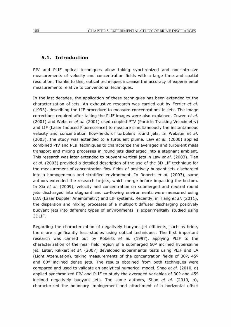
100 CHAPTER 5. EXPERIMENTAL STUDY OF BRINE DISCHARGES
5.1. Introduction
PIV and PLIF optical techniques allow taking synchronized and non-intrusive
measurements of velocity and concentration fields with a large time and spatial
resolution. Thanks to this, optical techniques increase the accuracy of experimental
measurements relative to conventional techniques.
In the last decades, the application of these techniques has been extended to the
characterization of jets. An exhaustive research was carried out by Ferrier et al.
(1993), describing the LIF procedure to measure concentrations in jets. The image
corrections required after taking the PLIF images were also explained. Cowen et al.
(2001) and Webster et al. (2001) used coupled PTV (Particle Tracking Velocimetry)
and LIF (Laser Induced Fluorescence) to measure simultaneously the instantaneous
velocity and concentration flow-fields of turbulent round jets. In Webster et al.
(2003), the study was extended to a turbulent plume. Law et al. (2000) applied
combined PIV and PLIF techniques to characterize the averaged and turbulent mass
transport and mixing processes in round jets discharged into a stagnant ambient.
This research was later extended to buoyant vertical jets in Law et al. (2003). Tian
et al. (2003) provided a detailed description of the use of the 3D LIF technique for
the measurement of concentration flow-fields of positively buoyant jets discharged
into a homogeneous and stratified environment. In Roberts et al. (2003), same
authors extended the research to jets, which merge before impacting the bottom.
In Xia et al. (2009), velocity and concentration on submerged and neutral round
jets discharged into stagnant and co-flowing environments were measured using
LDA (Laser Doppler Anemometry) and LIF systems. Recently, in Tiang et al. (2011),
the dispersion and mixing processes of a multiport diffuser discharging positively
buoyant jets into different types of environments is experimentally studied using
3DLIF.
Regarding the characterization of negatively buoyant jet effluents, such as brine,
there are significantly less studies using optical techniques. The first important
research was carried out by Roberts et al. (1997), applying PLIF to the
characterization of the near field region of a submerged 60º inclined hypersaline
jet. Later, Kikkert et al. (2007) developed experimental tests using PLIF and LA
(Light Attenuation), taking measurements of the concentration fields of 30º, 45º
and 60º inclined dense jets. The results obtained from both techniques were
compared and used to validate an analytical numerical model. Shao et al. (2010, a)
applied synchronized PIV and PLIF to study the averaged variables of 30º and 45º
inclined negatively buoyant jets. The same authors, Shao et al. (2010, b),
characterized the boundary impingement and attachment of a horizontal offset
CHAPTER 5. EXPERIMENTAL STUDY OF BRINE DISCHARGES 101
dense jet. An in-depth analysis of turbulent mass and momentum transport
processes was presented in Shao et al. (2009). Gungor et al. (2009) investigated
through 3D LIF, the behavior of a vertical negatively buoyant jet discharged into
dynamic environments.
However, these studies related to negatively buoyant jets give very few details of
the experimental methodology and criteria assumed to select the PLIF and PIV
parameters for the tests. Therefore, there is no published research describing the
procedure to apply these complex techniques to the characterization of brine jet
discharges. This type of flow presents special features that must be considered for
an accurate characterization.
To overcome this gap, the present chapter provides an exhaustive description of
the experimental procedure for using PIV and PLIF techniques to the study of this
type of flow, focusing on the main aspects to be considered for a good
accomplishment of the experiments. The test configuration, the instrumentation
and the PLIF and PIV techniques are briefly described first. Regarding PIV, the
criteria considered to select the seeding tracer particles and their density in flow
images are exposed. After that, it has been analyzed the relevance of the time
between pulses and the cross-correlation function to obtain reliable velocity
measurements. Concerning PLIF, the aspects taken into account to select the dye
tracer and concentration are firstly described. Next, the required image correction
and the estimation of the attenuation coefficients are described. After that, the
calibration procedure to transform fluorescence measurements into concentration
values is shown.
To finish, time series are displayed for various points within the flow trajectory,
determining the number of images before reaching the stationary state. Once the
images corresponding to this state are neglected, the convergence of statistics is
analyzed to ensure that the remainder number of images is enough for a statistical
representative characterization of the flow processes.
5.2. Experimental setup
The experiments were carried out in the Environmental Hydraulics Institute
(University of Cantabria, Spain). The experimental setup consisted of a 3×3×1 m3
test tank, simulating the receiving body, and a 1000 l plastic storage tank and a
100 l steel constant head tank, containing both the brine effluent.
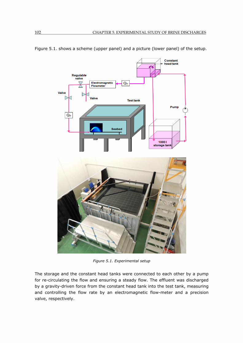
102 CHAPTER 5. EXPERIMENTAL STUDY OF BRINE DISCHARGES
Figure 5.1. shows a scheme (upper panel) and a picture (lower panel) of the setup.
Figure 5.1. Experimental setup
The storage and the constant head tanks were connected to each other by a pump
for re-circulating the flow and ensuring a steady flow. The effluent was discharged
by a gravity-driven force from the constant head tank into the test tank, measuring
and controlling the flow rate by an electromagnetic flow-meter and a precision
valve, respectively.
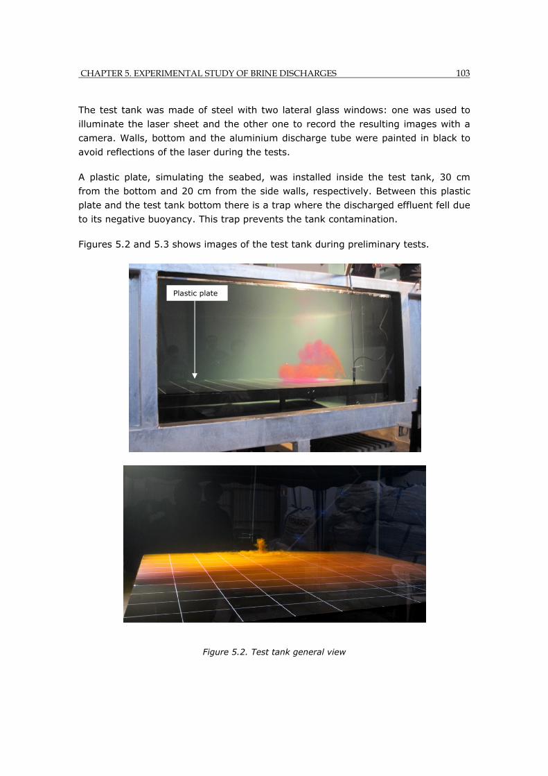
CHAPTER 5. EXPERIMENTAL STUDY OF BRINE DISCHARGES 103
The test tank was made of steel with two lateral glass windows: one was used to
illuminate the laser sheet and the other one to record the resulting images with a
camera. Walls, bottom and the aluminium discharge tube were painted in black to
avoid reflections of the laser during the tests.
A plastic plate, simulating the seabed, was installed inside the test tank, 30 cm
from the bottom and 20 cm from the side walls, respectively. Between this plastic
plate and the test tank bottom there is a trap where the discharged effluent fell due
to its negative buoyancy. This trap prevents the tank contamination.
Figures 5.2 and 5.3 shows images of the test tank during preliminary tests.
Figure 5.2. Test tank general view
Plastic plate
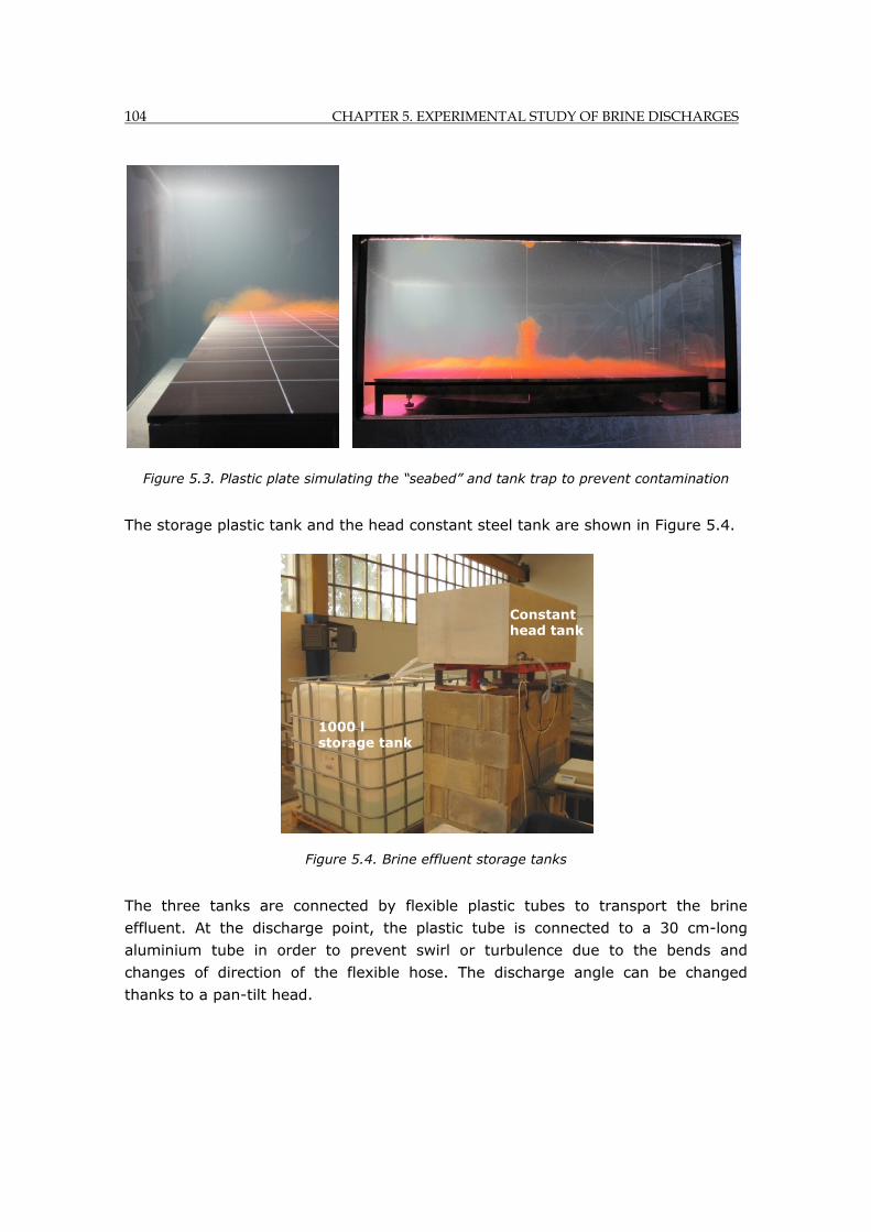
104 CHAPTER 5. EXPERIMENTAL STUDY OF BRINE DISCHARGES
Figure 5.3. Plastic plate simulating the “seabed” and tank trap to prevent contamination
The storage plastic tank and the head constant steel tank are shown in Figure 5.4.
Figure 5.4. Brine effluent storage tanks
The three tanks are connected by flexible plastic tubes to transport the brine
effluent. At the discharge point, the plastic tube is connected to a 30 cm-long
aluminium tube in order to prevent swirl or turbulence due to the bends and
changes of direction of the flexible hose. The discharge angle can be changed
thanks to a pan-tilt head.
Constant head tank
1000 l storage tank
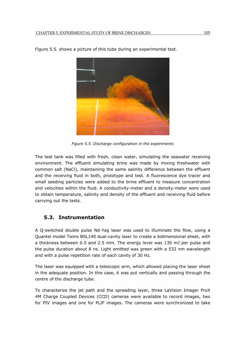
CHAPTER 5. EXPERIMENTAL STUDY OF BRINE DISCHARGES 105
Figure 5.5. shows a picture of this tube during an experimental test.
Figure 5.5. Discharge configuration in the experiments
The test tank was filled with fresh, clean water, simulating the seawater receiving
environment. The effluent simulating brine was made by mixing freshwater with
common salt (NaCl), maintaining the same salinity difference between the effluent
and the receiving fluid in both, prototype and test. A fluorescence dye tracer and
small seeding particles were added to the brine effluent to measure concentration
and velocities within the fluid. A conductivity-meter and a density-meter were used
to obtain temperature, salinity and density of the effluent and receiving fluid before
carrying out the tests.
5.3. Instrumentation
A Q-switched double pulse Nd-Yag laser was used to illuminate the flow, using a
Quantel model Twins BSL140 dual-cavity laser to create a bidimensional sheet, with
a thickness between 0.5 and 2.5 mm. The energy level was 130 mJ per pulse and
the pulse duration about 8 ns. Light emitted was green with a 532 nm wavelength
and with a pulse repetition rate of each cavity of 30 Hz.
The laser was equipped with a telescopic arm, which allowed placing the laser sheet
in the adequate position. In this case, it was put vertically and passing through the
centre of the discharge tube.
To characterize the jet path and the spreading layer, three LaVision Imager ProX
4M Charge Coupled Devices (CCD) cameras were available to record images, two
for PIV images and one for PLIF images. The cameras were synchronized to take
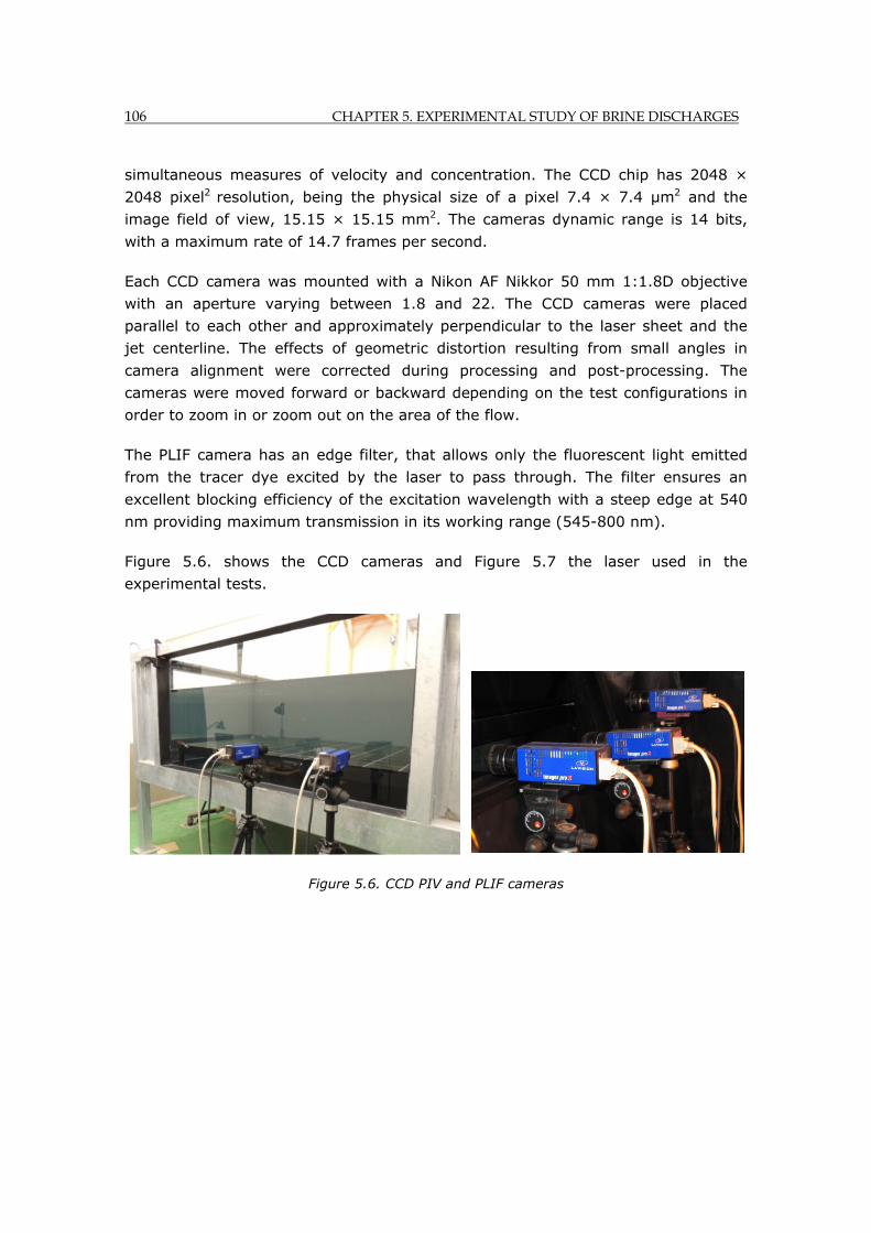
106 CHAPTER 5. EXPERIMENTAL STUDY OF BRINE DISCHARGES
simultaneous measures of velocity and concentration. The CCD chip has 2048 ×
2048 pixel2 resolution, being the physical size of a pixel 7.4 × 7.4 µm2 and the
image field of view, 15.15 × 15.15 mm2. The cameras dynamic range is 14 bits,
with a maximum rate of 14.7 frames per second.
Each CCD camera was mounted with a Nikon AF Nikkor 50 mm 1:1.8D objective
with an aperture varying between 1.8 and 22. The CCD cameras were placed
parallel to each other and approximately perpendicular to the laser sheet and the
jet centerline. The effects of geometric distortion resulting from small angles in
camera alignment were corrected during processing and post-processing. The
cameras were moved forward or backward depending on the test configurations in
order to zoom in or zoom out on the area of the flow.
The PLIF camera has an edge filter, that allows only the fluorescent light emitted
from the tracer dye excited by the laser to pass through. The filter ensures an
excellent blocking efficiency of the excitation wavelength with a steep edge at 540
nm providing maximum transmission in its working range (545-800 nm).
Figure 5.6. shows the CCD cameras and Figure 5.7 the laser used in the
experimental tests.
Figure 5.6. CCD PIV and PLIF cameras
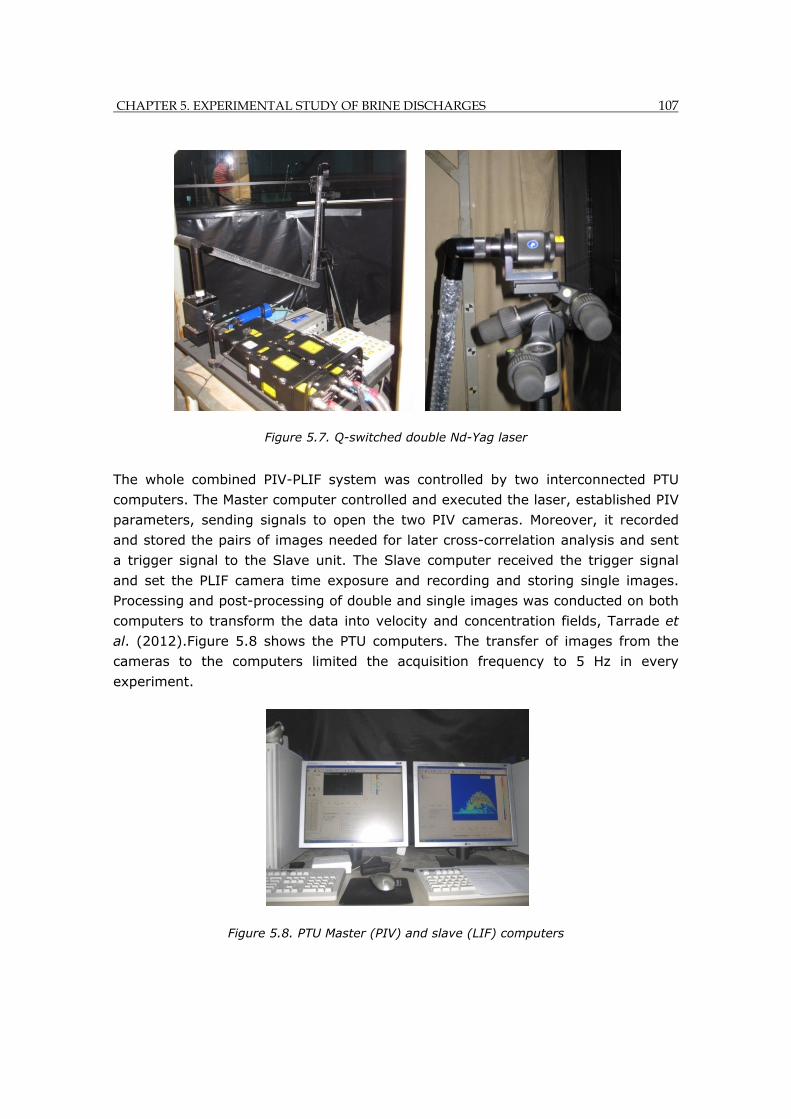
CHAPTER 5. EXPERIMENTAL STUDY OF BRINE DISCHARGES 107
Figure 5.7. Q-switched double Nd-Yag laser
The whole combined PIV-PLIF system was controlled by two interconnected PTU
computers. The Master computer controlled and executed the laser, established PIV
parameters, sending signals to open the two PIV cameras. Moreover, it recorded
and stored the pairs of images needed for later cross-correlation analysis and sent
a trigger signal to the Slave unit. The Slave computer received the trigger signal
and set the PLIF camera time exposure and recording and storing single images.
Processing and post-processing of double and single images was conducted on both
computers to transform the data into velocity and concentration fields, Tarrade et
al. (2012).Figure 5.8 shows the PTU computers. The transfer of images from the
cameras to the computers limited the acquisition frequency to 5 Hz in every
experiment.
Figure 5.8. PTU Master (PIV) and slave (LIF) computers
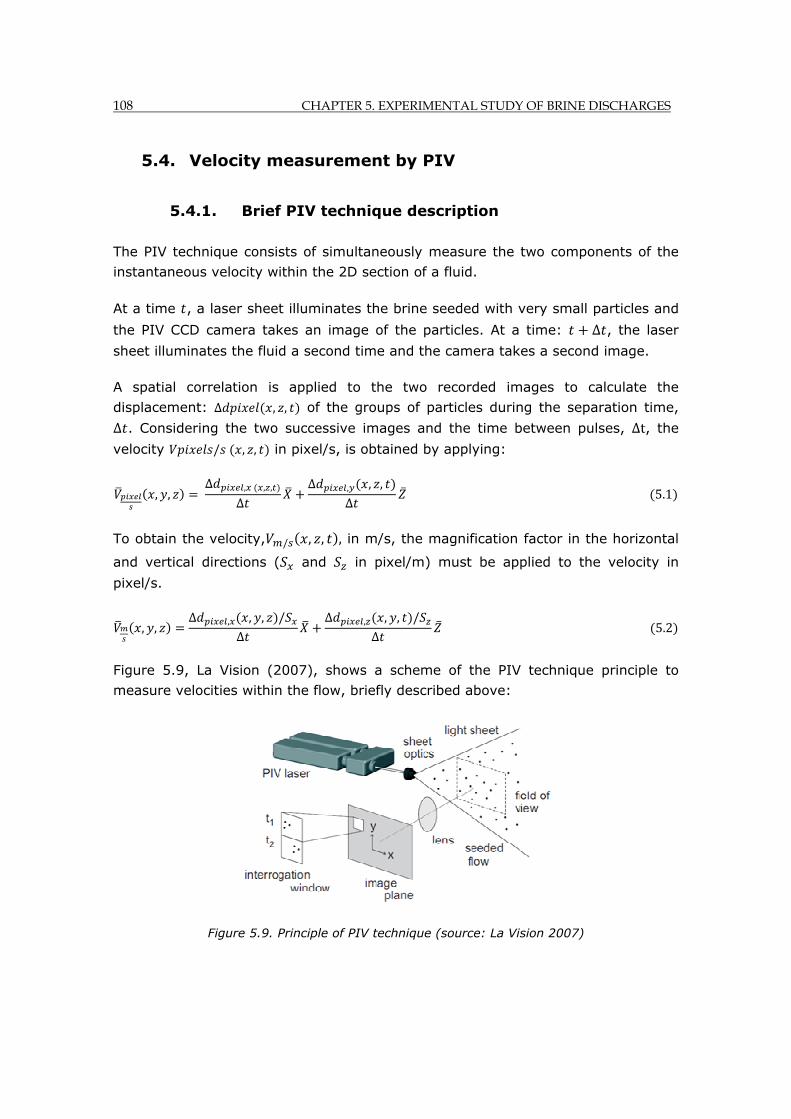
108 CHAPTER 5. EXPERIMENTAL STUDY OF BRINE DISCHARGES
5.4. Velocity measurement by PIV
5.4.1. Brief PIV technique description
The PIV technique consists of simultaneously measure the two components of the
instantaneous velocity within the 2D section of a fluid.
At a time , a laser sheet illuminates the brine seeded with very small particles and
the PIV CCD camera takes an image of the particles. At a time: ∆ , the laser
sheet illuminates the fluid a second time and the camera takes a second image.
A spatial correlation is applied to the two recorded images to calculate the
displacement: ∆ , , of the groups of particles during the separation time,
∆ . Considering the two successive images and the time between pulses, ∆t, the
velocity / , , in pixel/s, is obtained by applying:
, , ∆ , , ,
∆∆ , , ,
∆ 5.1
To obtain the velocity, / , , , in m/s, the magnification factor in the horizontal
and vertical directions ( and in pixel/m) must be applied to the velocity in
pixel/s.
, ,∆ , , , /
∆∆ , , , /
∆ 5.2
Figure 5.9, La Vision (2007), shows a scheme of the PIV technique principle to
measure velocities within the flow, briefly described above:
Figure 5.9. Principle of PIV technique (source: La Vision 2007)
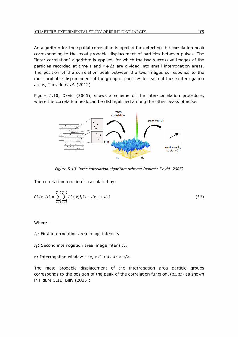
CHAPTER 5. EXPERIMENTAL STUDY OF BRINE DISCHARGES 109
An algorithm for the spatial correlation is applied for detecting the correlation peak
corresponding to the most probable displacement of particles between pulses. The
“inter-correlation” algorithm is applied, for which the two successive images of the
particles recorded at time and ∆ are divided into small interrogation areas.
The position of the correlation peak between the two images corresponds to the
most probable displacement of the group of particles for each of these interrogation
areas, Tarrade et al. (2012).
Figure 5.10, David (2005), shows a scheme of the inter-correlation procedure,
where the correlation peak can be distinguished among the other peaks of noise.
Figure 5.10. Inter-correlation algorithm scheme (source: David, 2005)
The correlation function is calculated by:
, , , 5.3
Where:
: First interrogation area image intensity.
: Second interrogation area image intensity.
: Interrogation window size, /2 , /2.
The most probable displacement of the interrogation area particle groups
corresponds to the position of the peak of the correlation function , , as shown
in Figure 5.11, Billy (2005):
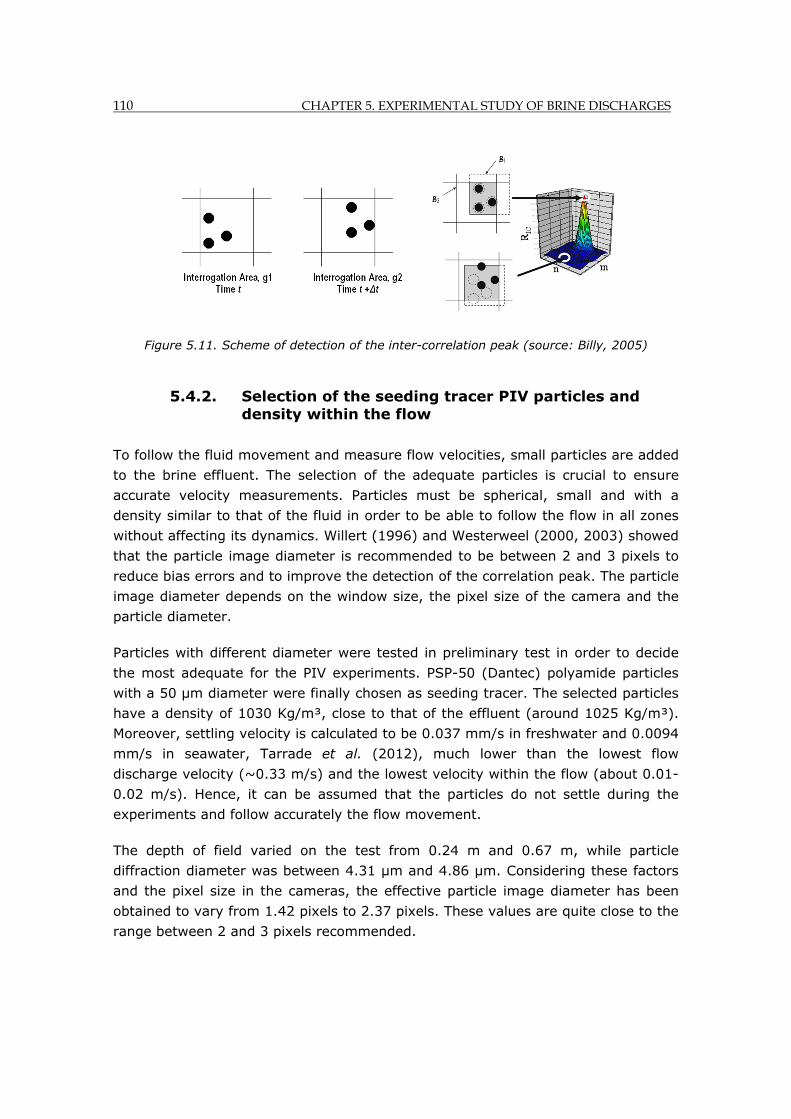
110 CHAPTER 5. EXPERIMENTAL STUDY OF BRINE DISCHARGES
Figure 5.11. Scheme of detection of the inter-correlation peak (source: Billy, 2005)
5.4.2. Selection of the seeding tracer PIV particles and density within the flow
To follow the fluid movement and measure flow velocities, small particles are added
to the brine effluent. The selection of the adequate particles is crucial to ensure
accurate velocity measurements. Particles must be spherical, small and with a
density similar to that of the fluid in order to be able to follow the flow in all zones
without affecting its dynamics. Willert (1996) and Westerweel (2000, 2003) showed
that the particle image diameter is recommended to be between 2 and 3 pixels to
reduce bias errors and to improve the detection of the correlation peak. The particle
image diameter depends on the window size, the pixel size of the camera and the
particle diameter.
Particles with different diameter were tested in preliminary test in order to decide
the most adequate for the PIV experiments. PSP-50 (Dantec) polyamide particles
with a 50 μm diameter were finally chosen as seeding tracer. The selected particles
have a density of 1030 Kg/m³, close to that of the effluent (around 1025 Kg/m³).
Moreover, settling velocity is calculated to be 0.037 mm/s in freshwater and 0.0094
mm/s in seawater, Tarrade et al. (2012), much lower than the lowest flow
discharge velocity (~0.33 m/s) and the lowest velocity within the flow (about 0.01-
0.02 m/s). Hence, it can be assumed that the particles do not settle during the
experiments and follow accurately the flow movement.
The depth of field varied on the test from 0.24 m and 0.67 m, while particle
diffraction diameter was between 4.31 μm and 4.86 μm. Considering these factors
and the pixel size in the cameras, the effective particle image diameter has been
obtained to vary from 1.42 pixels to 2.37 pixels. These values are quite close to the
range between 2 and 3 pixels recommended.
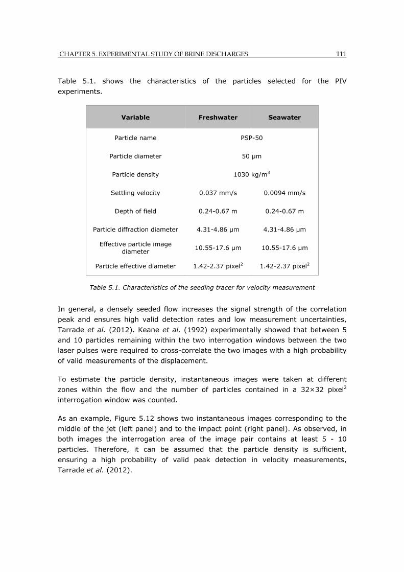
CHAPTER 5. EXPERIMENTAL STUDY OF BRINE DISCHARGES 111
Table 5.1. shows the characteristics of the particles selected for the PIV
experiments.
Variable Freshwater Seawater
Particle name PSP-50
Particle diameter 50 µm
Particle density 1030 kg/m3
Settling velocity 0.037 mm/s 0.0094 mm/s
Depth of field 0.24-0.67 m 0.24-0.67 m
Particle diffraction diameter 4.31-4.86 µm 4.31-4.86 µm
Effective particle image diameter
10.55-17.6 µm 10.55-17.6 µm
Particle effective diameter 1.42-2.37 pixel2 1.42-2.37 pixel2
Table 5.1. Characteristics of the seeding tracer for velocity measurement
In general, a densely seeded flow increases the signal strength of the correlation
peak and ensures high valid detection rates and low measurement uncertainties,
Tarrade et al. (2012). Keane et al. (1992) experimentally showed that between 5
and 10 particles remaining within the two interrogation windows between the two
laser pulses were required to cross-correlate the two images with a high probability
of valid measurements of the displacement.
To estimate the particle density, instantaneous images were taken at different
zones within the flow and the number of particles contained in a 32×32 pixel2
interrogation window was counted.
As an example, Figure 5.12 shows two instantaneous images corresponding to the
middle of the jet (left panel) and to the impact point (right panel). As observed, in
both images the interrogation area of the image pair contains at least 5 - 10
particles. Therefore, it can be assumed that the particle density is sufficient,
ensuring a high probability of valid peak detection in velocity measurements,
Tarrade et al. (2012).
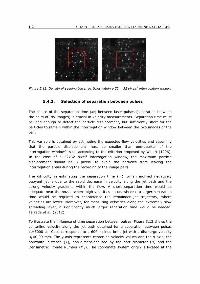
112 CHAPTER 5. EXPERIMENTAL STUDY OF BRINE DISCHARGES
Figure 5.12. Density of seeding tracer particles within a 32 × 32 pixels2 interrogation window
5.4.3. Selection of separation between pulses
The choice of the separation time ( ) between laser pulses (separation between
the pairs of PIV images) is crucial in velocity measurements. Separation time must
be long enough to detect the particle displacement, but sufficiently short for the
particles to remain within the interrogation window between the two images of the
pair.
This variable is obtained by estimating the expected flow velocities and assuming
that the particle displacement must be smaller than one-quarter of the
interrogation window’s size, according to the criterion proposed by Willert (1996).
In the case of a 32x32 pixel2 interrogation window, the maximum particle
displacement should be 8 pixels, to avoid the particles from leaving the
interrogation areas during the recording of the image pairs.
The difficulty in estimating the separation time ( ) for an inclined negatively
buoyant jet is due to the rapid decrease in velocity along the jet path and the
strong velocity gradients within the flow. A short separation time would be
adequate near the nozzle where high velocities occur, whereas a larger separation
time would be required to characterize the remainder jet trajectory, where
velocities are lower. Moreover, for measuring velocities along the extremely slow
spreading layer, a significantly much larger separation time would be needed,
Tarrade et al. (2012).
To illustrate the influence of time separation between pulses, Figure 5.13 shows the
centerline velocity along the jet path obtained for a separation between pulses
=5000 µs. Case corresponds to a 60º inclined brine jet with a discharge velocity
Uo=0.99 m/s. The y-axis represents centerline velocity values and the x-axis, the
horizontal distance ( ), non-dimensionalized by the port diameter ( ) and the
Densimetric Froude Number ( ). The coordinate system origin is located at the
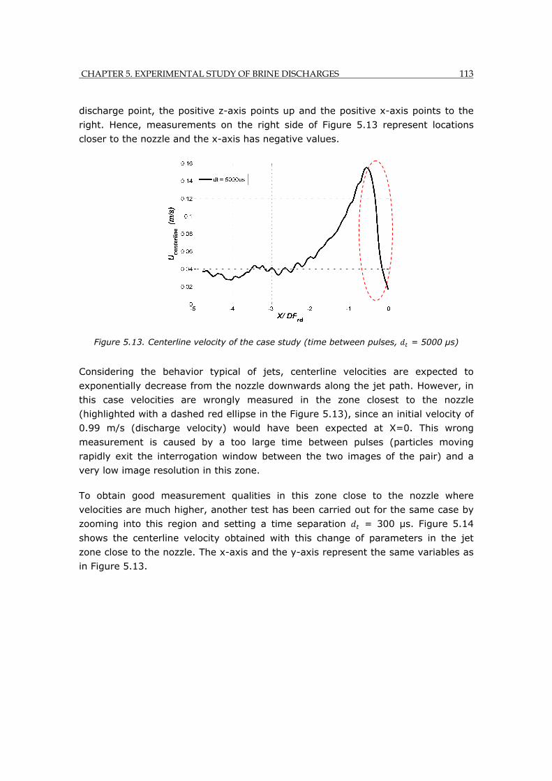
CHAPTER 5. EXPERIMENTAL STUDY OF BRINE DISCHARGES 113
discharge point, the positive z-axis points up and the positive x-axis points to the
right. Hence, measurements on the right side of Figure 5.13 represent locations
closer to the nozzle and the x-axis has negative values.
Figure 5.13. Centerline velocity of the case study (time between pulses, = 5000 µs)
Considering the behavior typical of jets, centerline velocities are expected to
exponentially decrease from the nozzle downwards along the jet path. However, in
this case velocities are wrongly measured in the zone closest to the nozzle
(highlighted with a dashed red ellipse in the Figure 5.13), since an initial velocity of
0.99 m/s (discharge velocity) would have been expected at X=0. This wrong
measurement is caused by a too large time between pulses (particles moving
rapidly exit the interrogation window between the two images of the pair) and a
very low image resolution in this zone.
To obtain good measurement qualities in this zone close to the nozzle where
velocities are much higher, another test has been carried out for the same case by
zooming into this region and setting a time separation = 300 µs. Figure 5.14
shows the centerline velocity obtained with this change of parameters in the jet
zone close to the nozzle. The x-axis and the y-axis represent the same variables as
in Figure 5.13.
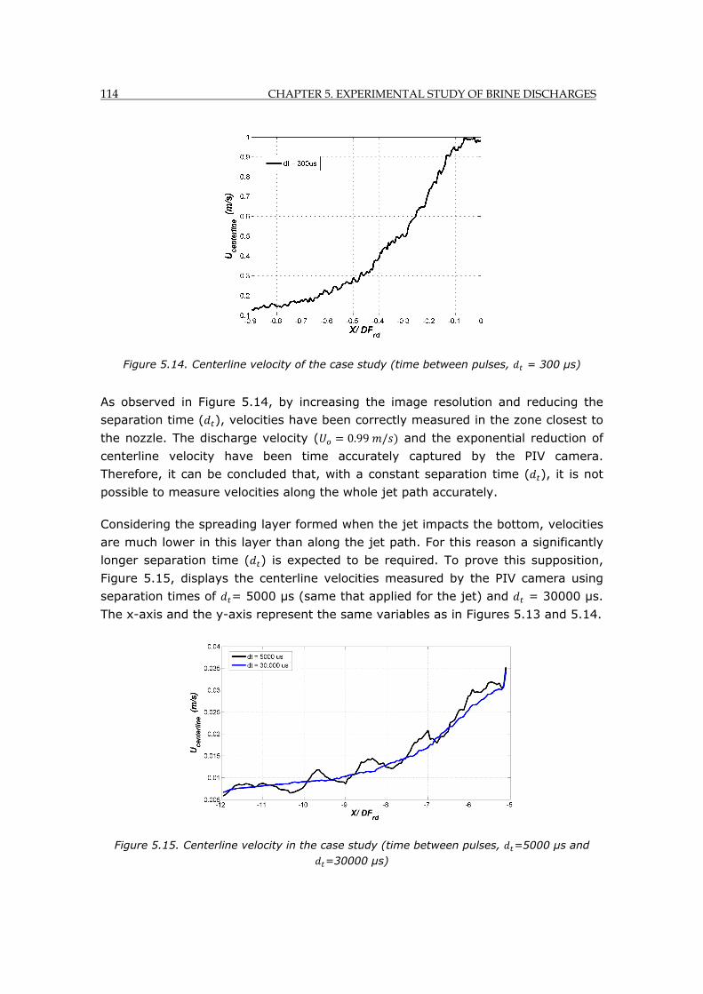
114 CHAPTER 5. EXPERIMENTAL STUDY OF BRINE DISCHARGES
Figure 5.14. Centerline velocity of the case study (time between pulses, = 300 µs)
As observed in Figure 5.14, by increasing the image resolution and reducing the
separation time ( ), velocities have been correctly measured in the zone closest to
the nozzle. The discharge velocity ( 0.99 / and the exponential reduction of
centerline velocity have been time accurately captured by the PIV camera.
Therefore, it can be concluded that, with a constant separation time ( ), it is not
possible to measure velocities along the whole jet path accurately.
Considering the spreading layer formed when the jet impacts the bottom, velocities
are much lower in this layer than along the jet path. For this reason a significantly
longer separation time ( ) is expected to be required. To prove this supposition,
Figure 5.15, displays the centerline velocities measured by the PIV camera using
separation times of = 5000 µs (same that applied for the jet) and = 30000 µs.
The x-axis and the y-axis represent the same variables as in Figures 5.13 and 5.14.
Figure 5.15. Centerline velocity in the case study (time between pulses, =5000 µs and =30000 µs)
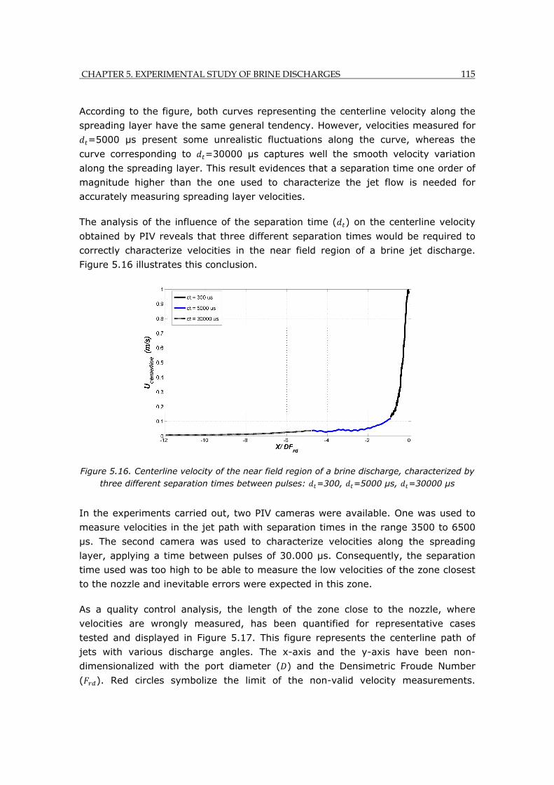
CHAPTER 5. EXPERIMENTAL STUDY OF BRINE DISCHARGES 115
According to the figure, both curves representing the centerline velocity along the
spreading layer have the same general tendency. However, velocities measured for
=5000 µs present some unrealistic fluctuations along the curve, whereas the
curve corresponding to =30000 µs captures well the smooth velocity variation
along the spreading layer. This result evidences that a separation time one order of
magnitude higher than the one used to characterize the jet flow is needed for
accurately measuring spreading layer velocities.
The analysis of the influence of the separation time ( ) on the centerline velocity
obtained by PIV reveals that three different separation times would be required to
correctly characterize velocities in the near field region of a brine jet discharge.
Figure 5.16 illustrates this conclusion.
Figure 5.16. Centerline velocity of the near field region of a brine discharge, characterized by three different separation times between pulses: =300, =5000 µs, =30000 µs
In the experiments carried out, two PIV cameras were available. One was used to
measure velocities in the jet path with separation times in the range 3500 to 6500
µs. The second camera was used to characterize velocities along the spreading
layer, applying a time between pulses of 30.000 µs. Consequently, the separation
time used was too high to be able to measure the low velocities of the zone closest
to the nozzle and inevitable errors were expected in this zone.
As a quality control analysis, the length of the zone close to the nozzle, where
velocities are wrongly measured, has been quantified for representative cases
tested and displayed in Figure 5.17. This figure represents the centerline path of
jets with various discharge angles. The x-axis and the y-axis have been non-
dimensionalized with the port diameter ( ) and the Densimetric Froude Number
( ). Red circles symbolize the limit of the non-valid velocity measurements.
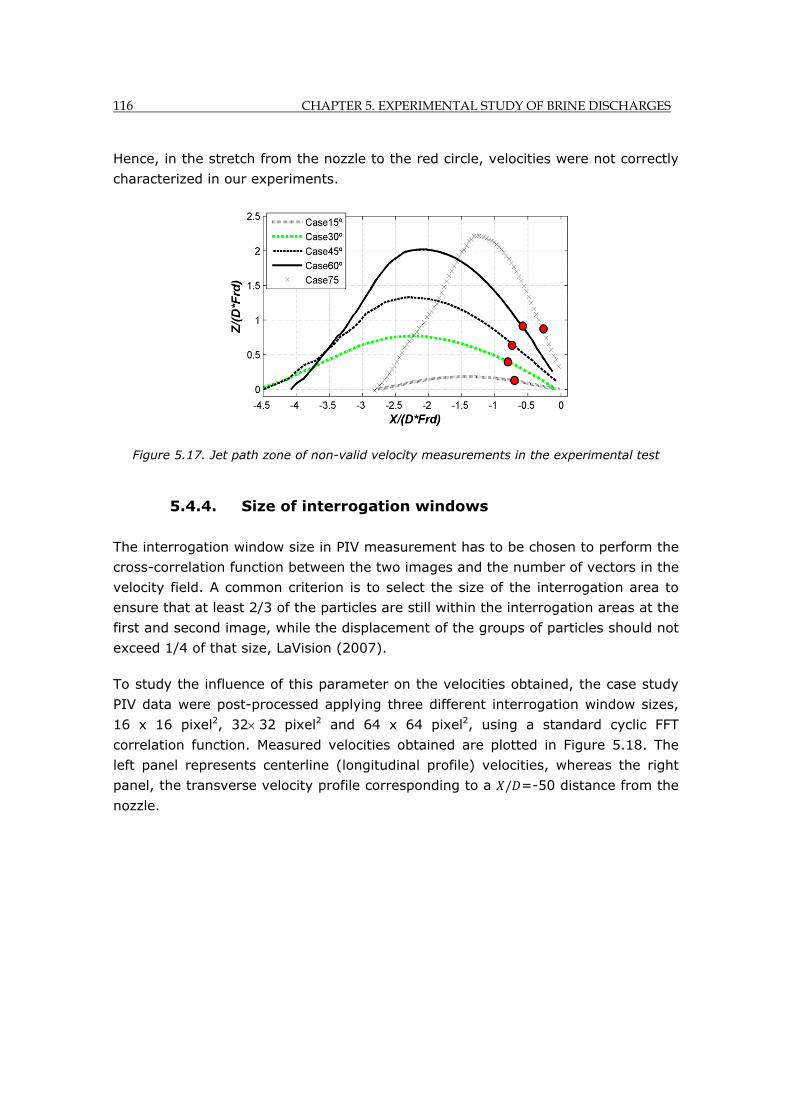
116 CHAPTER 5. EXPERIMENTAL STUDY OF BRINE DISCHARGES
Hence, in the stretch from the nozzle to the red circle, velocities were not correctly
characterized in our experiments.
Figure 5.17. Jet path zone of non-valid velocity measurements in the experimental test
5.4.4. Size of interrogation windows
The interrogation window size in PIV measurement has to be chosen to perform the
cross-correlation function between the two images and the number of vectors in the
velocity field. A common criterion is to select the size of the interrogation area to
ensure that at least 2/3 of the particles are still within the interrogation areas at the
first and second image, while the displacement of the groups of particles should not
exceed 1/4 of that size, LaVision (2007).
To study the influence of this parameter on the velocities obtained, the case study
PIV data were post-processed applying three different interrogation window sizes,
16 x 16 pixel2, 3232 pixel2 and 64 x 64 pixel2, using a standard cyclic FFT
correlation function. Measured velocities obtained are plotted in Figure 5.18. The
left panel represents centerline (longitudinal profile) velocities, whereas the right
panel, the transverse velocity profile corresponding to a / =-50 distance from the
nozzle.
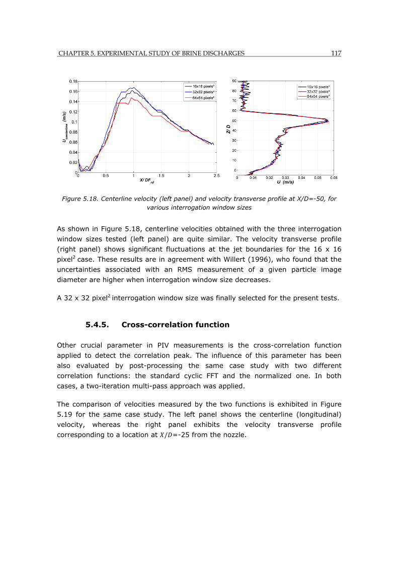
CHAPTER 5. EXPERIMENTAL STUDY OF BRINE DISCHARGES 117
Figure 5.18. Centerline velocity (left panel) and velocity transverse profile at X/D=-50, for various interrogation window sizes
As shown in Figure 5.18, centerline velocities obtained with the three interrogation
window sizes tested (left panel) are quite similar. The velocity transverse profile
(right panel) shows significant fluctuations at the jet boundaries for the 16 x 16
pixel2 case. These results are in agreement with Willert (1996), who found that the
uncertainties associated with an RMS measurement of a given particle image
diameter are higher when interrogation window size decreases.
A 32 x 32 pixel2 interrogation window size was finally selected for the present tests.
5.4.5. Cross-correlation function
Other crucial parameter in PIV measurements is the cross-correlation function
applied to detect the correlation peak. The influence of this parameter has been
also evaluated by post-processing the same case study with two different
correlation functions: the standard cyclic FFT and the normalized one. In both
cases, a two-iteration multi-pass approach was applied.
The comparison of velocities measured by the two functions is exhibited in Figure
5.19 for the same case study. The left panel shows the centerline (longitudinal)
velocity, whereas the right panel exhibits the velocity transverse profile
corresponding to a location at / =-25 from the nozzle.
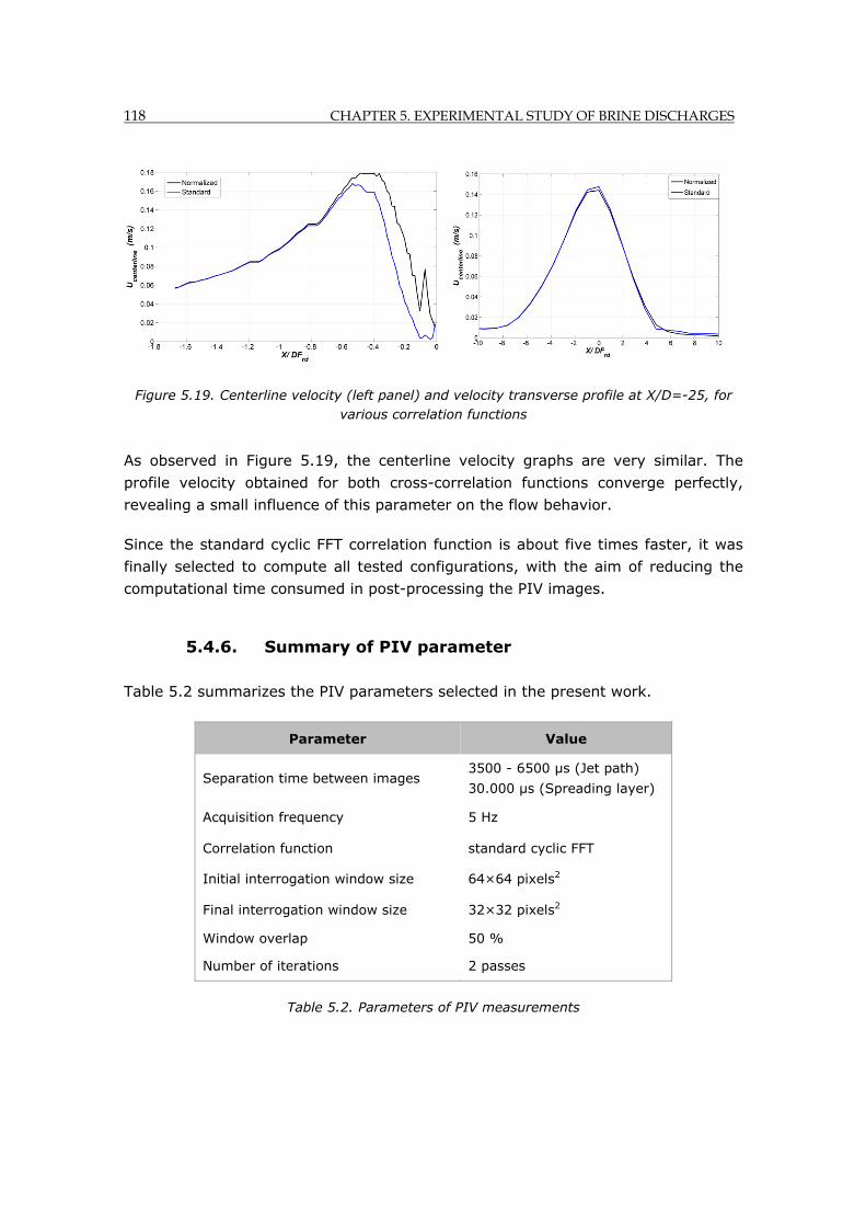
118 CHAPTER 5. EXPERIMENTAL STUDY OF BRINE DISCHARGES
Figure 5.19. Centerline velocity (left panel) and velocity transverse profile at X/D=-25, for various correlation functions
As observed in Figure 5.19, the centerline velocity graphs are very similar. The
profile velocity obtained for both cross-correlation functions converge perfectly,
revealing a small influence of this parameter on the flow behavior.
Since the standard cyclic FFT correlation function is about five times faster, it was
finally selected to compute all tested configurations, with the aim of reducing the
computational time consumed in post-processing the PIV images.
5.4.6. Summary of PIV parameter
Table 5.2 summarizes the PIV parameters selected in the present work.
Parameter Value
Separation time between images 3500 - 6500 µs (Jet path)
30.000 µs (Spreading layer)
Acquisition frequency 5 Hz
Correlation function standard cyclic FFT
Initial interrogation window size 64×64 pixels2
Final interrogation window size 32×32 pixels2
Window overlap 50 %
Number of iterations 2 passes
Table 5.2. Parameters of PIV measurements
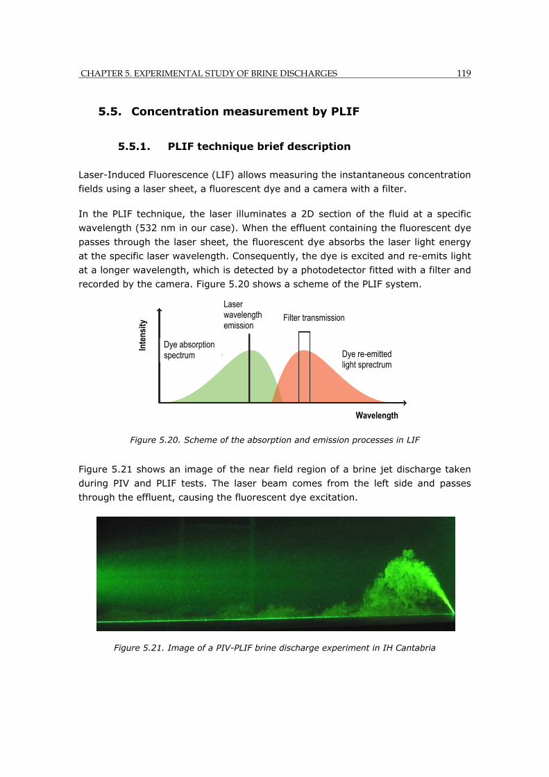
CHAPTER 5. EXPERIMENTAL STUDY OF BRINE DISCHARGES 119
5.5. Concentration measurement by PLIF
5.5.1. PLIF technique brief description
Laser-Induced Fluorescence (LIF) allows measuring the instantaneous concentration
fields using a laser sheet, a fluorescent dye and a camera with a filter.
In the PLIF technique, the laser illuminates a 2D section of the fluid at a specific
wavelength (532 nm in our case). When the effluent containing the fluorescent dye
passes through the laser sheet, the fluorescent dye absorbs the laser light energy
at the specific laser wavelength. Consequently, the dye is excited and re-emits light
at a longer wavelength, which is detected by a photodetector fitted with a filter and
recorded by the camera. Figure 5.20 shows a scheme of the PLIF system.
Figure 5.20. Scheme of the absorption and emission processes in LIF
Figure 5.21 shows an image of the near field region of a brine jet discharge taken
during PIV and PLIF tests. The laser beam comes from the left side and passes
through the effluent, causing the fluorescent dye excitation.
Figure 5.21. Image of a PIV-PLIF brine discharge experiment in IH Cantabria
Laser wavelength emission
Filter transmission
Dye re-emitted light sprectrum
Dye absorption spectrum
Wavelength
Inte
nsity
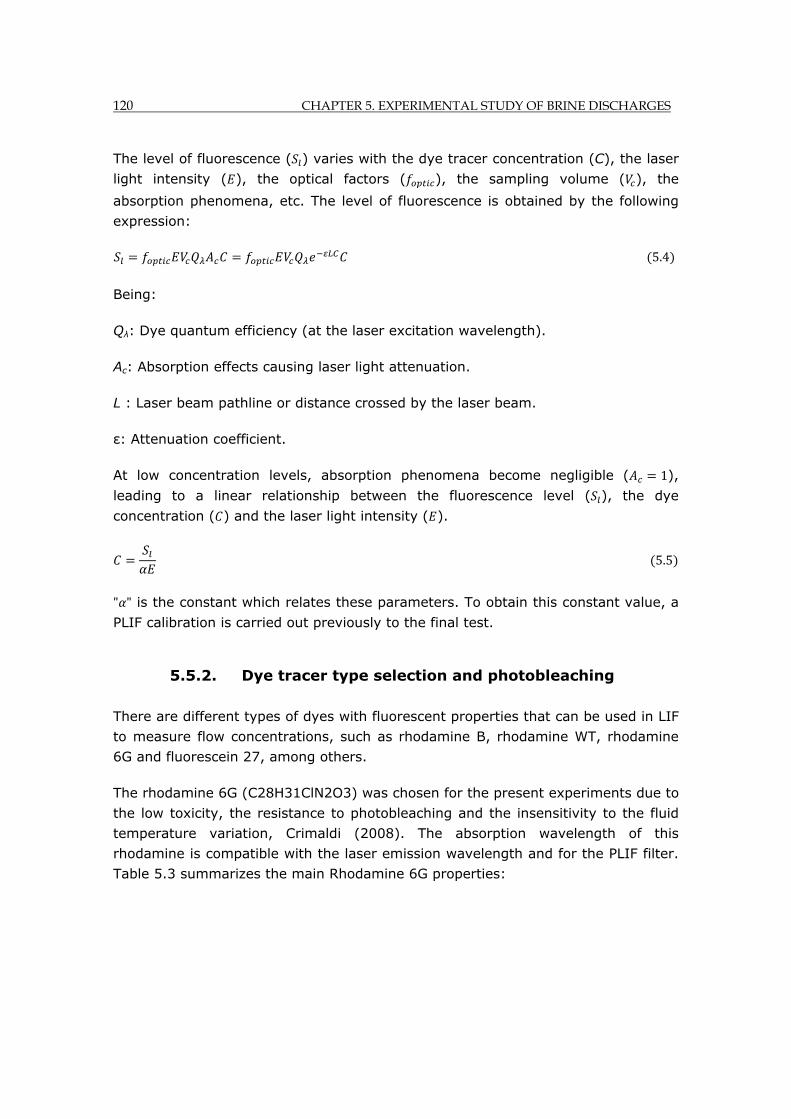
120 CHAPTER 5. EXPERIMENTAL STUDY OF BRINE DISCHARGES
The level of fluorescence ( ) varies with the dye tracer concentration (C), the laser
light intensity ( ), the optical factors ( ), the sampling volume ( ), the
absorption phenomena, etc. The level of fluorescence is obtained by the following
expression:
5.4
Being:
Qλ: Dye quantum efficiency (at the laser excitation wavelength).
Ac: Absorption effects causing laser light attenuation.
L : Laser beam pathline or distance crossed by the laser beam.
ε: Attenuation coefficient.
At low concentration levels, absorption phenomena become negligible ( 1),
leading to a linear relationship between the fluorescence level ( ), the dye
concentration ( ) and the laser light intensity ( ).
5.5
" " is the constant which relates these parameters. To obtain this constant value, a
PLIF calibration is carried out previously to the final test.
5.5.2. Dye tracer type selection and photobleaching
There are different types of dyes with fluorescent properties that can be used in LIF
to measure flow concentrations, such as rhodamine B, rhodamine WT, rhodamine
6G and fluorescein 27, among others.
The rhodamine 6G (C28H31ClN2O3) was chosen for the present experiments due to
the low toxicity, the resistance to photobleaching and the insensitivity to the fluid
temperature variation, Crimaldi (2008). The absorption wavelength of this
rhodamine is compatible with the laser emission wavelength and for the PLIF filter.
Table 5.3 summarizes the main Rhodamine 6G properties:
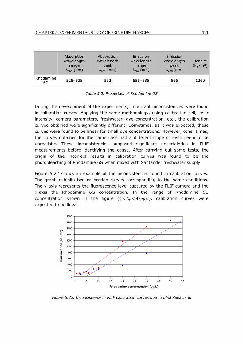
CHAPTER 5. EXPERIMENTAL STUDY OF BRINE DISCHARGES 121
Table 5.3. Properties of Rhodamine 6G
During the development of the experiments, important inconsistencies were found
in calibration curves. Applying the same methodology, using calibration cell, laser
intensity, camera parameters, freshwater, dye concentration, etc., the calibration
curved obtained were significantly different. Sometimes, as it was expected, these
curves were found to be linear for small dye concentrations. However, other times,
the curves obtained for the same case had a different slope or even seem to be
unrealistic. These inconsistencies supposed significant uncertainties in PLIF
measurements before identifying the cause. After carrying out some tests, the
origin of the incorrect results in calibration curves was found to be the
photobleaching of Rhodamine 6G when mixed with Santander freshwater supply.
Figure 5.22 shows an example of the inconsistencies found in calibration curves.
The graph exhibits two calibration curves corresponding to the same conditions.
The y-axis represents the fluorescence level captured by the PLIF camera and the
x-axis the Rhodamine 6G concentration. In the range of Rhodamine 6G
concentration shown in the figure (0 45 / ), calibration curves were
expected to be linear.
Figure 5.22. Inconsistency in PLIF calibration curves due to photobleaching
0
200
400
600
800
1000
1200
1400
1600
1800
2000
0 5 10 15 20 25 30 35 40 45
Flu
ore
sc
en
ce
(co
un
ts)
Rhodamine concentration (µg/L)
Absorption wavelength
range λabs (nm)
Absorption wavelength
peak λabs (nm)
Emission wavelength
range λemi (nm)
Emission wavelength
peak λemi (nm)
Density (kg/m³)
Rhodamine 6G
525–535 532 555–585 566 1260
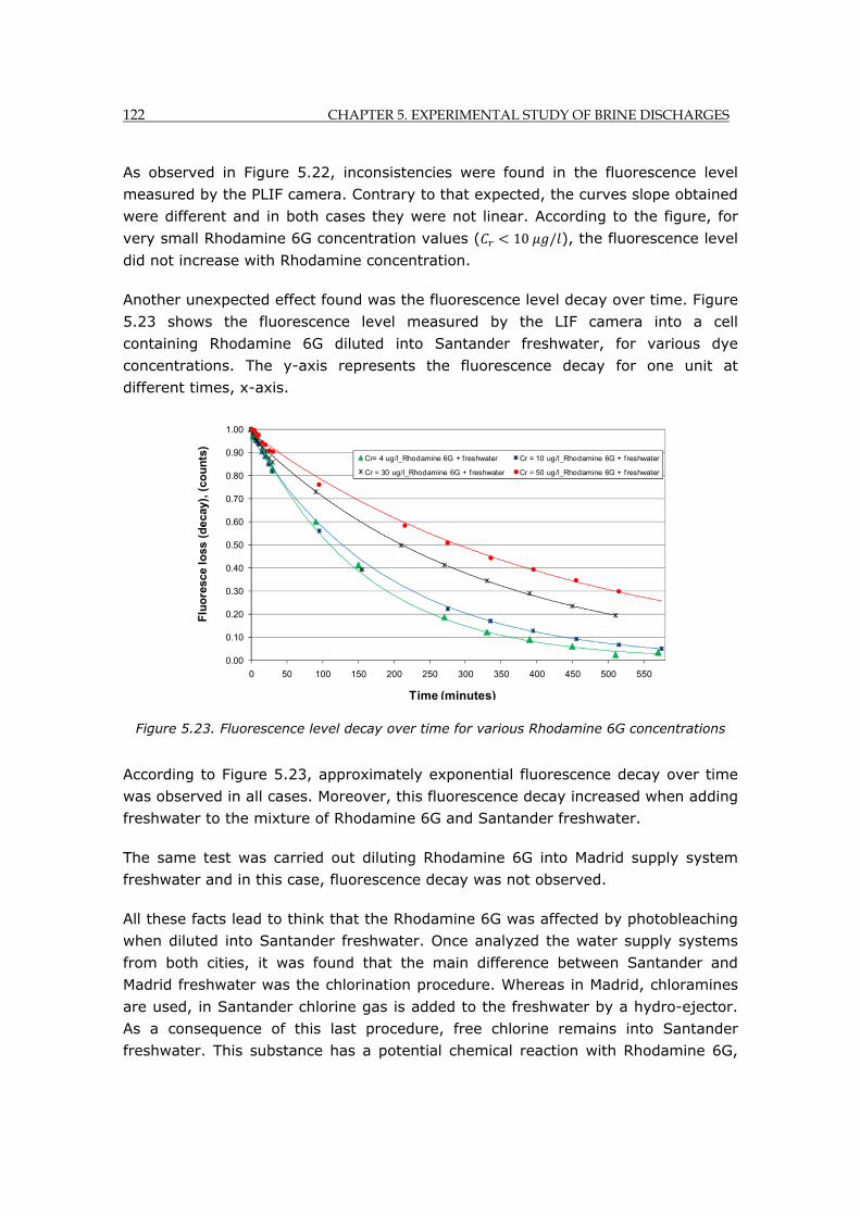
122 CHAPTER 5. EXPERIMENTAL STUDY OF BRINE DISCHARGES
As observed in Figure 5.22, inconsistencies were found in the fluorescence level
measured by the PLIF camera. Contrary to that expected, the curves slope obtained
were different and in both cases they were not linear. According to the figure, for
very small Rhodamine 6G concentration values ( 10 / ), the fluorescence level
did not increase with Rhodamine concentration.
Another unexpected effect found was the fluorescence level decay over time. Figure
5.23 shows the fluorescence level measured by the LIF camera into a cell
containing Rhodamine 6G diluted into Santander freshwater, for various dye
concentrations. The y-axis represents the fluorescence decay for one unit at
different times, x-axis.
Figure 5.23. Fluorescence level decay over time for various Rhodamine 6G concentrations
According to Figure 5.23, approximately exponential fluorescence decay over time
was observed in all cases. Moreover, this fluorescence decay increased when adding
freshwater to the mixture of Rhodamine 6G and Santander freshwater.
The same test was carried out diluting Rhodamine 6G into Madrid supply system
freshwater and in this case, fluorescence decay was not observed.
All these facts lead to think that the Rhodamine 6G was affected by photobleaching
when diluted into Santander freshwater. Once analyzed the water supply systems
from both cities, it was found that the main difference between Santander and
Madrid freshwater was the chlorination procedure. Whereas in Madrid, chloramines
are used, in Santander chlorine gas is added to the freshwater by a hydro-ejector.
As a consequence of this last procedure, free chlorine remains into Santander
freshwater. This substance has a potential chemical reaction with Rhodamine 6G,
0.00
0.10
0.20
0.30
0.40
0.50
0.60
0.70
0.80
0.90
1.00
0 50 100 150 200 250 300 350 400 450 500 550
Flu
ore
sce
loss
(d
ecay
), (
cou
nts
)
Time (minutes)
Cr= 4 ug/l_Rhodamine 6G + f reshwater Cr = 10 ug/l_Rhodamine 6G + f reshwater
Cr = 30 ug/l_Rhodamine 6G + f reshwater Cr = 50 ug/l_Rhodamine 6G + f reshwater
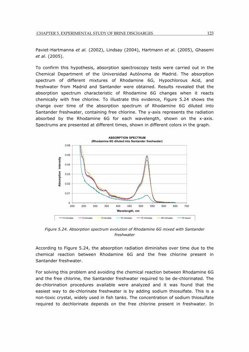
CHAPTER 5. EXPERIMENTAL STUDY OF BRINE DISCHARGES 123
Paviet-Hartmanna et al. (2002), Lindsay (2004), Hartmann et al. (2005), Ghasemi
et al. (2005).
To confirm this hypothesis, absorption spectroscopy tests were carried out in the
Chemical Department of the Universidad Autónoma de Madrid. The absorption
spectrum of different mixtures of Rhodamine 6G, Hypochlorous Acid, and
freshwater from Madrid and Santander were obtained. Results revealed that the
absorption spectrum characteristic of Rhodamine 6G changes when it reacts
chemically with free chlorine. To illustrate this evidence, Figure 5.24 shows the
change over time of the absorption spectrum of Rhodamine 6G diluted into
Santander freshwater, containing free chlorine. The y-axis represents the radiation
absorbed by the Rhodamine 6G for each wavelength, shown on the x-axis.
Spectrums are presented at different times, shown in different colors in the graph.
Figure 5.24. Absorption spectrum evolution of Rhodamine 6G mixed with Santander freshwater
According to Figure 5.24, the absorption radiation diminishes over time due to the
chemical reaction between Rhodamine 6G and the free chlorine present in
Santander freshwater.
For solving this problem and avoiding the chemical reaction between Rhodamine 6G
and the free chlorine, the Santander freshwater required to be de-chlorinated. The
de-chlorination procedures available were analyzed and it was found that the
easiest way to de-chlorinate freshwater is by adding sodium thiosulfate. This is a
non-toxic crystal, widely used in fish tanks. The concentration of sodium thiosulfate
required to dechlorinate depends on the free chlorine present in freshwater. In
0
0.01
0.02
0.03
0.04
0.05
0.06
200 250 300 350 400 450 500 550 600 650 700
Ab
so
rpti
on
in
ten
sit
y
Wavelength, nm
ABSORPTION SPECTRUM (Rhodamine 6G diluted into Santander freshwater)
0 minutes 2 minutes 5 minutes 10 minutes 15 minutes 40 minutes 15 hours
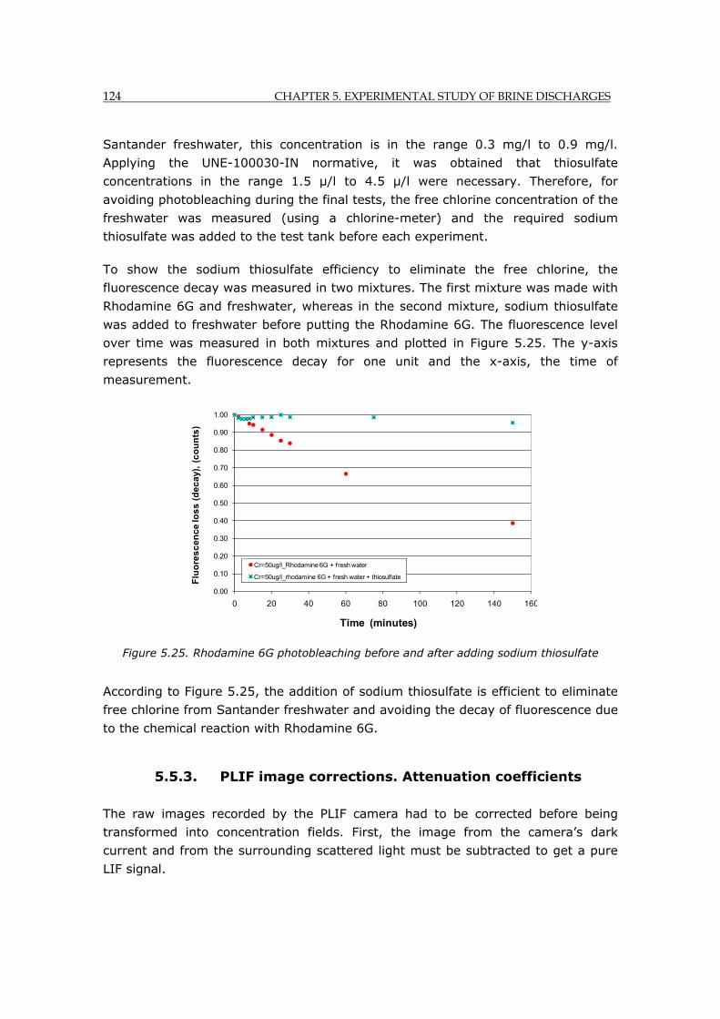
124 CHAPTER 5. EXPERIMENTAL STUDY OF BRINE DISCHARGES
Santander freshwater, this concentration is in the range 0.3 mg/l to 0.9 mg/l.
Applying the UNE-100030-IN normative, it was obtained that thiosulfate
concentrations in the range 1.5 μ/l to 4.5 μ/l were necessary. Therefore, for
avoiding photobleaching during the final tests, the free chlorine concentration of the
freshwater was measured (using a chlorine-meter) and the required sodium
thiosulfate was added to the test tank before each experiment.
To show the sodium thiosulfate efficiency to eliminate the free chlorine, the
fluorescence decay was measured in two mixtures. The first mixture was made with
Rhodamine 6G and freshwater, whereas in the second mixture, sodium thiosulfate
was added to freshwater before putting the Rhodamine 6G. The fluorescence level
over time was measured in both mixtures and plotted in Figure 5.25. The y-axis
represents the fluorescence decay for one unit and the x-axis, the time of
measurement.
Figure 5.25. Rhodamine 6G photobleaching before and after adding sodium thiosulfate
According to Figure 5.25, the addition of sodium thiosulfate is efficient to eliminate
free chlorine from Santander freshwater and avoiding the decay of fluorescence due
to the chemical reaction with Rhodamine 6G.
5.5.3. PLIF image corrections. Attenuation coefficients
The raw images recorded by the PLIF camera had to be corrected before being
transformed into concentration fields. First, the image from the camera’s dark
current and from the surrounding scattered light must be subtracted to get a pure
LIF signal.
0.00
0.10
0.20
0.30
0.40
0.50
0.60
0.70
0.80
0.90
1.00
0 20 40 60 80 100 120 140 160
Flu
ore
sc
en
ce
los
s (
de
ca
y),
(co
un
ts)
Time (minutes)
Cr=50ug/l_Rhodamine 6G + fresh water
Cr=50ug/l_rhodamine 6G + fresh water + thiosulfate
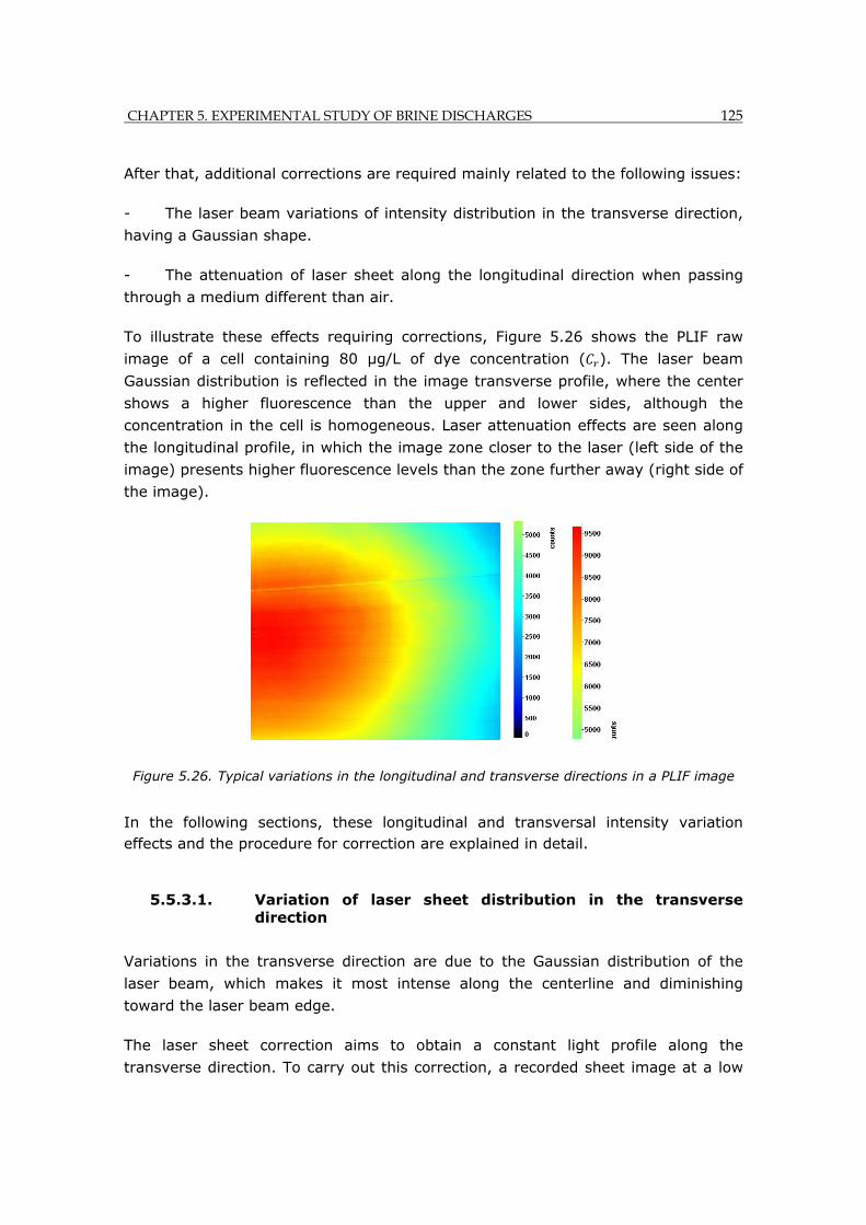
CHAPTER 5. EXPERIMENTAL STUDY OF BRINE DISCHARGES 125
After that, additional corrections are required mainly related to the following issues:
- The laser beam variations of intensity distribution in the transverse direction,
having a Gaussian shape.
- The attenuation of laser sheet along the longitudinal direction when passing
through a medium different than air.
To illustrate these effects requiring corrections, Figure 5.26 shows the PLIF raw
image of a cell containing 80 µg/L of dye concentration ( ). The laser beam
Gaussian distribution is reflected in the image transverse profile, where the center
shows a higher fluorescence than the upper and lower sides, although the
concentration in the cell is homogeneous. Laser attenuation effects are seen along
the longitudinal profile, in which the image zone closer to the laser (left side of the
image) presents higher fluorescence levels than the zone further away (right side of
the image).
Figure 5.26. Typical variations in the longitudinal and transverse directions in a PLIF image
In the following sections, these longitudinal and transversal intensity variation effects and the procedure for correction are explained in detail.
5.5.3.1. Variation of laser sheet distribution in the transverse direction
Variations in the transverse direction are due to the Gaussian distribution of the
laser beam, which makes it most intense along the centerline and diminishing
toward the laser beam edge.
The laser sheet correction aims to obtain a constant light profile along the
transverse direction. To carry out this correction, a recorded sheet image at a low
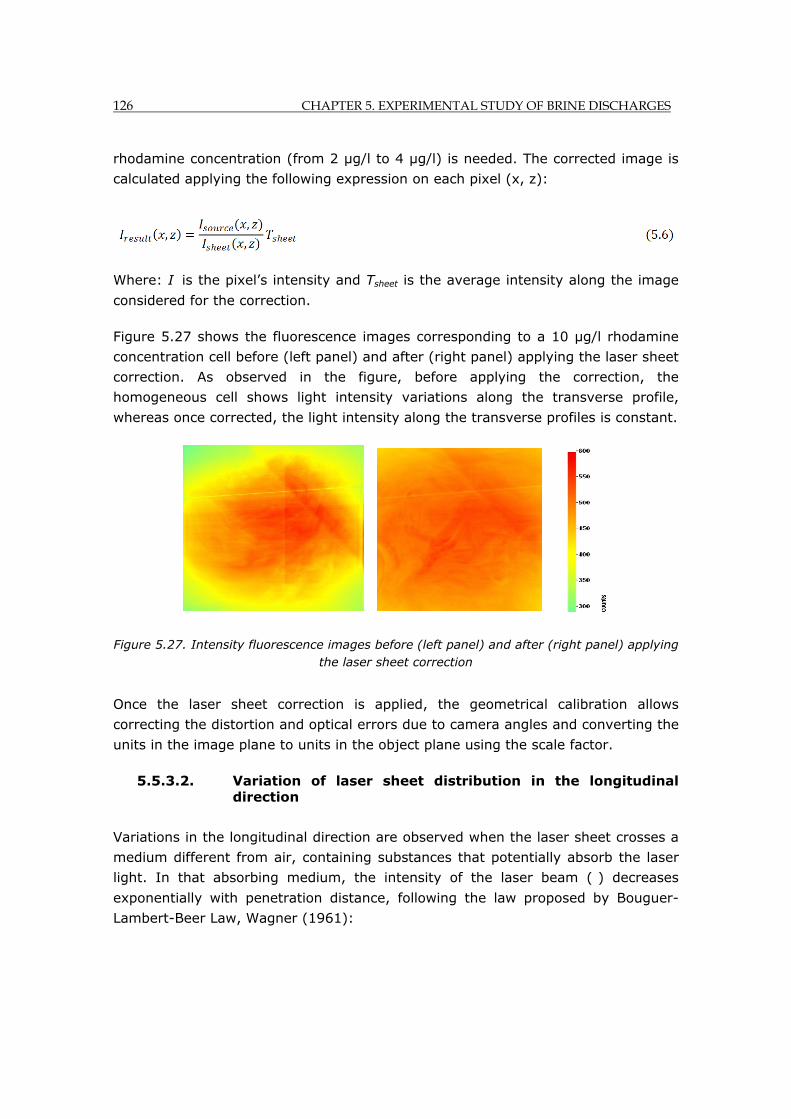
126 CHAPTER 5. EXPERIMENTAL STUDY OF BRINE DISCHARGES
rhodamine concentration (from 2 µg/l to 4 µg/l) is needed. The corrected image is
calculated applying the following expression on each pixel (x, z):
Where: I is the pixel’s intensity and Tsheet is the average intensity along the image
considered for the correction.
Figure 5.27 shows the fluorescence images corresponding to a 10 µg/l rhodamine
concentration cell before (left panel) and after (right panel) applying the laser sheet
correction. As observed in the figure, before applying the correction, the
homogeneous cell shows light intensity variations along the transverse profile,
whereas once corrected, the light intensity along the transverse profiles is constant.
Figure 5.27. Intensity fluorescence images before (left panel) and after (right panel) applying the laser sheet correction
Once the laser sheet correction is applied, the geometrical calibration allows
correcting the distortion and optical errors due to camera angles and converting the
units in the image plane to units in the object plane using the scale factor.
5.5.3.2. Variation of laser sheet distribution in the longitudinal direction
Variations in the longitudinal direction are observed when the laser sheet crosses a
medium different from air, containing substances that potentially absorb the laser
light. In that absorbing medium, the intensity of the laser beam ( ) decreases
exponentially with penetration distance, following the law proposed by Bouguer-
Lambert-Beer Law, Wagner (1961):
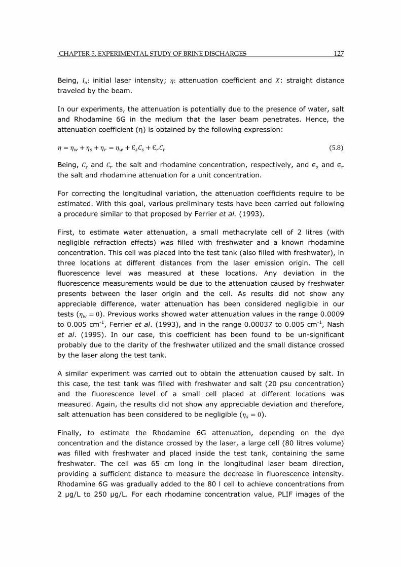
CHAPTER 5. EXPERIMENTAL STUDY OF BRINE DISCHARGES 127
Being, : initial laser intensity; : attenuation coefficient and : straight distance
traveled by the beam.
In our experiments, the attenuation is potentially due to the presence of water, salt
and Rhodamine 6G in the medium that the laser beam penetrates. Hence, the
attenuation coefficient (η) is obtained by the following expression:
Є Є 5.8
Being, and the salt and rhodamine concentration, respectively, and and
the salt and rhodamine attenuation for a unit concentration.
For correcting the longitudinal variation, the attenuation coefficients require to be
estimated. With this goal, various preliminary tests have been carried out following
a procedure similar to that proposed by Ferrier et al. (1993).
First, to estimate water attenuation, a small methacrylate cell of 2 litres (with
negligible refraction effects) was filled with freshwater and a known rhodamine
concentration. This cell was placed into the test tank (also filled with freshwater), in
three locations at different distances from the laser emission origin. The cell
fluorescence level was measured at these locations. Any deviation in the
fluorescence measurements would be due to the attenuation caused by freshwater
presents between the laser origin and the cell. As results did not show any
appreciable difference, water attenuation has been considered negligible in our
tests ( 0). Previous works showed water attenuation values in the range 0.0009
to 0.005 cm-1, Ferrier et al. (1993), and in the range 0.00037 to 0.005 cm-1, Nash
et al. (1995). In our case, this coefficient has been found to be un-significant
probably due to the clarity of the freshwater utilized and the small distance crossed
by the laser along the test tank.
A similar experiment was carried out to obtain the attenuation caused by salt. In
this case, the test tank was filled with freshwater and salt (20 psu concentration)
and the fluorescence level of a small cell placed at different locations was
measured. Again, the results did not show any appreciable deviation and therefore,
salt attenuation has been considered to be negligible ( 0).
Finally, to estimate the Rhodamine 6G attenuation, depending on the dye
concentration and the distance crossed by the laser, a large cell (80 litres volume)
was filled with freshwater and placed inside the test tank, containing the same
freshwater. The cell was 65 cm long in the longitudinal laser beam direction,
providing a sufficient distance to measure the decrease in fluorescence intensity.
Rhodamine 6G was gradually added to the 80 l cell to achieve concentrations from
2 µg/L to 250 µg/L. For each rhodamine concentration value, PLIF images of the
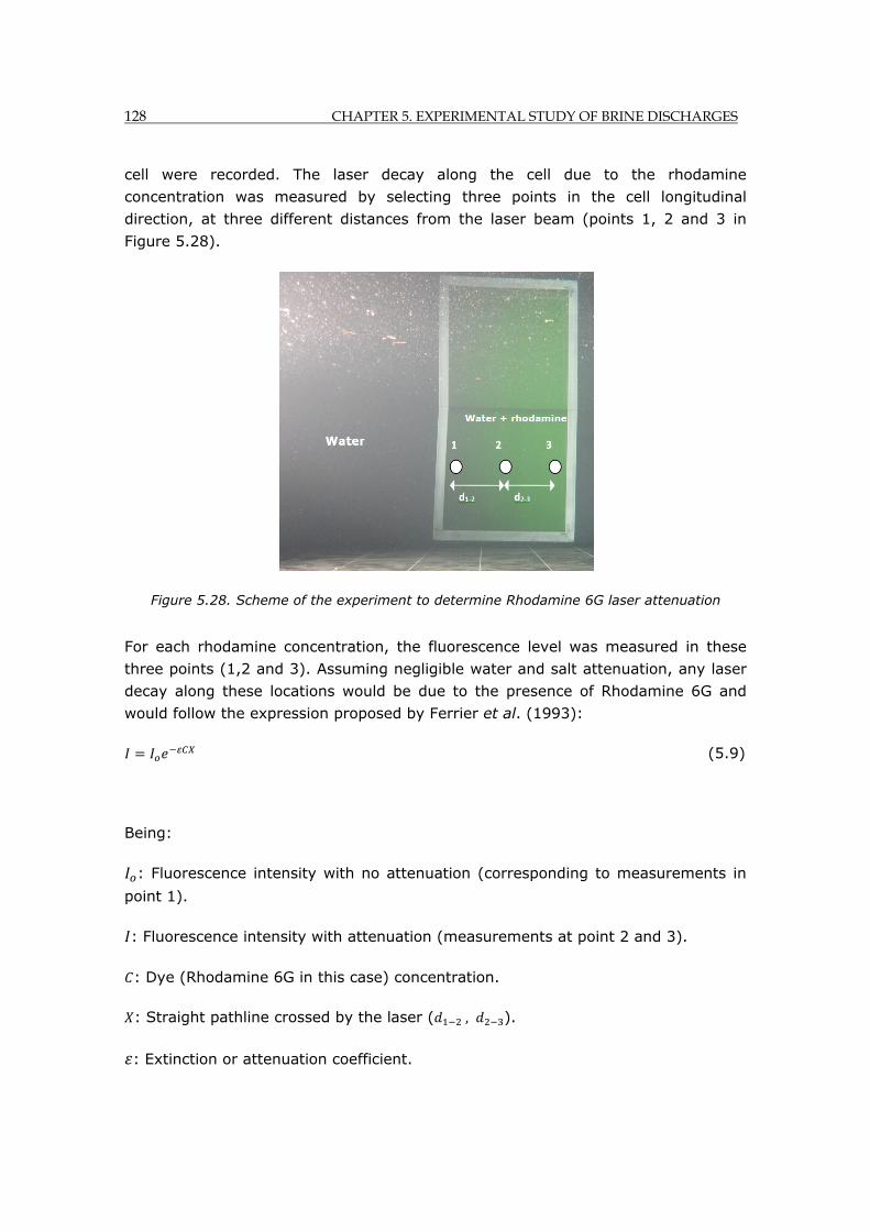
128 CHAPTER 5. EXPERIMENTAL STUDY OF BRINE DISCHARGES
cell were recorded. The laser decay along the cell due to the rhodamine
concentration was measured by selecting three points in the cell longitudinal
direction, at three different distances from the laser beam (points 1, 2 and 3 in
Figure 5.28).
Figure 5.28. Scheme of the experiment to determine Rhodamine 6G laser attenuation
For each rhodamine concentration, the fluorescence level was measured in these
three points (1,2 and 3). Assuming negligible water and salt attenuation, any laser
decay along these locations would be due to the presence of Rhodamine 6G and
would follow the expression proposed by Ferrier et al. (1993):
(5.9)
Being:
: Fluorescence intensity with no attenuation (corresponding to measurements in
point 1).
: Fluorescence intensity with attenuation (measurements at point 2 and 3).
: Dye (Rhodamine 6G in this case) concentration.
: Straight pathline crossed by the laser ( , ).
: Extinction or attenuation coefficient.
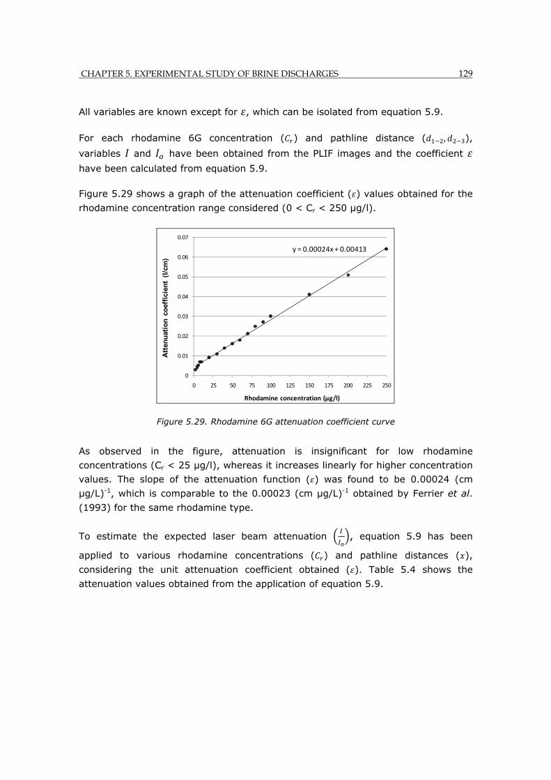
CHAPTER 5. EXPERIMENTAL STUDY OF BRINE DISCHARGES 129
All variables are known except for , which can be isolated from equation 5.9.
For each rhodamine 6G concentration ( ) and pathline distance ( , ),
variables and have been obtained from the PLIF images and the coefficient have been calculated from equation 5.9.
Figure 5.29 shows a graph of the attenuation coefficient ( ) values obtained for the
rhodamine concentration range considered (0 < Cr < 250 µg/l).
Figure 5.29. Rhodamine 6G attenuation coefficient curve
As observed in the figure, attenuation is insignificant for low rhodamine
concentrations (Cr < 25 µg/l), whereas it increases linearly for higher concentration
values. The slope of the attenuation function ( ) was found to be 0.00024 (cm
µg/L)-1, which is comparable to the 0.00023 (cm µg/L)-1 obtained by Ferrier et al.
(1993) for the same rhodamine type.
To estimate the expected laser beam attenuation , equation 5.9 has been
applied to various rhodamine concentrations ( ) and pathline distances ( ),
considering the unit attenuation coefficient obtained ( ). Table 5.4 shows the
attenuation values obtained from the application of equation 5.9.
y = 0.00024x + 0.00413
0
0.01
0.02
0.03
0.04
0.05
0.06
0.07
0 25 50 75 100 125 150 175 200 225 250
Att
enu
atio
n c
oef
fici
ent
(I/c
m)
Rhodamine concentration (µg/l)
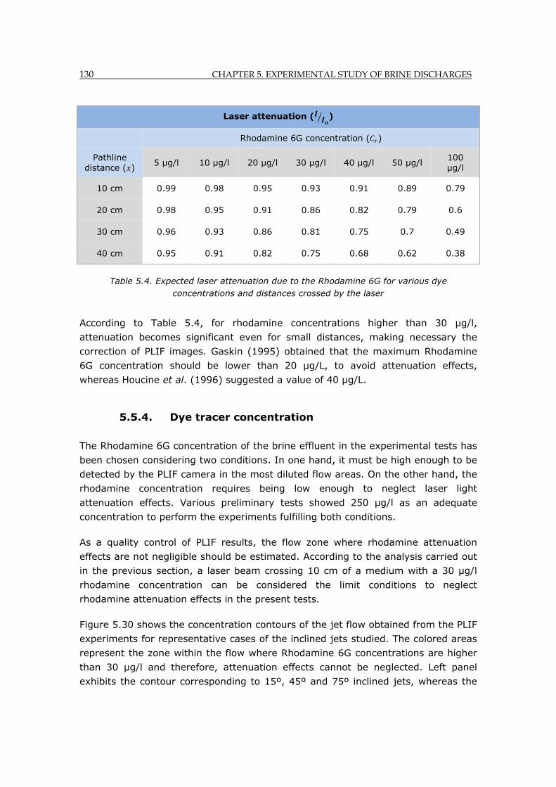
130 CHAPTER 5. EXPERIMENTAL STUDY OF BRINE DISCHARGES
Laser attenuation ( )
Rhodamine 6G concentration ( )
Pathline distance ( ) 5 µg/l 10 µg/l 20 µg/l 30 µg/l 40 µg/l 50 µg/l
100 µg/l
10 cm 0.99 0.98 0.95 0.93 0.91 0.89 0.79
20 cm 0.98 0.95 0.91 0.86 0.82 0.79 0.6
30 cm 0.96 0.93 0.86 0.81 0.75 0.7 0.49
40 cm 0.95 0.91 0.82 0.75 0.68 0.62 0.38
Table 5.4. Expected laser attenuation due to the Rhodamine 6G for various dye concentrations and distances crossed by the laser
According to Table 5.4, for rhodamine concentrations higher than 30 µg/l,
attenuation becomes significant even for small distances, making necessary the
correction of PLIF images. Gaskin (1995) obtained that the maximum Rhodamine
6G concentration should be lower than 20 µg/L, to avoid attenuation effects,
whereas Houcine et al. (1996) suggested a value of 40 µg/L.
5.5.4. Dye tracer concentration
The Rhodamine 6G concentration of the brine effluent in the experimental tests has
been chosen considering two conditions. In one hand, it must be high enough to be
detected by the PLIF camera in the most diluted flow areas. On the other hand, the
rhodamine concentration requires being low enough to neglect laser light
attenuation effects. Various preliminary tests showed 250 µg/l as an adequate
concentration to perform the experiments fulfilling both conditions.
As a quality control of PLIF results, the flow zone where rhodamine attenuation
effects are not negligible should be estimated. According to the analysis carried out
in the previous section, a laser beam crossing 10 cm of a medium with a 30 µg/l
rhodamine concentration can be considered the limit conditions to neglect
rhodamine attenuation effects in the present tests.
Figure 5.30 shows the concentration contours of the jet flow obtained from the PLIF
experiments for representative cases of the inclined jets studied. The colored areas
represent the zone within the flow where Rhodamine 6G concentrations are higher
than 30 µg/l and therefore, attenuation effects cannot be neglected. Left panel
exhibits the contour corresponding to 15º, 45º and 75º inclined jets, whereas the
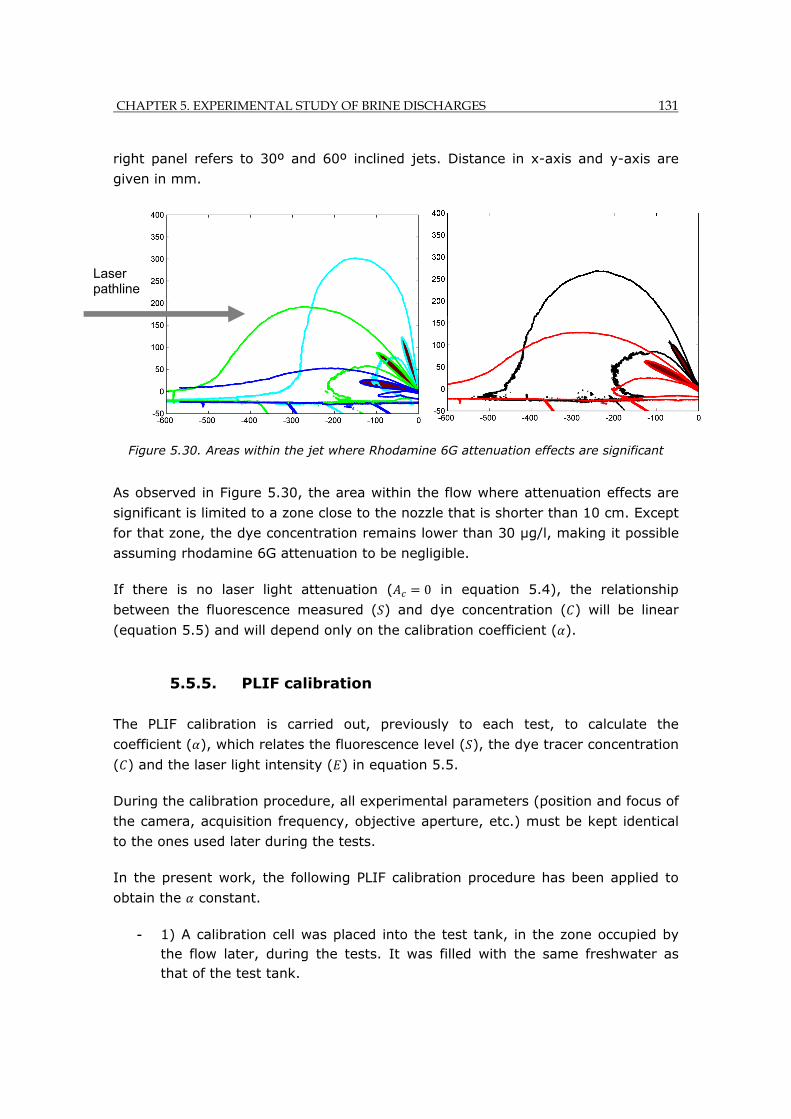
CHAPTER 5. EXPERIMENTAL STUDY OF BRINE DISCHARGES 131
right panel refers to 30º and 60º inclined jets. Distance in x-axis and y-axis are
given in mm.
Figure 5.30. Areas within the jet where Rhodamine 6G attenuation effects are significant
As observed in Figure 5.30, the area within the flow where attenuation effects are
significant is limited to a zone close to the nozzle that is shorter than 10 cm. Except
for that zone, the dye concentration remains lower than 30 µg/l, making it possible
assuming rhodamine 6G attenuation to be negligible.
If there is no laser light attenuation ( 0 in equation 5.4), the relationship
between the fluorescence measured ( ) and dye concentration ( ) will be linear
(equation 5.5) and will depend only on the calibration coefficient ( ).
5.5.5. PLIF calibration
The PLIF calibration is carried out, previously to each test, to calculate the
coefficient ( ), which relates the fluorescence level ( ), the dye tracer concentration
( ) and the laser light intensity ( ) in equation 5.5.
During the calibration procedure, all experimental parameters (position and focus of
the camera, acquisition frequency, objective aperture, etc.) must be kept identical
to the ones used later during the tests.
In the present work, the following PLIF calibration procedure has been applied to
obtain the constant.
- 1) A calibration cell was placed into the test tank, in the zone occupied by the flow later, during the tests. It was filled with the same freshwater as that of the test tank.
Laser pathline
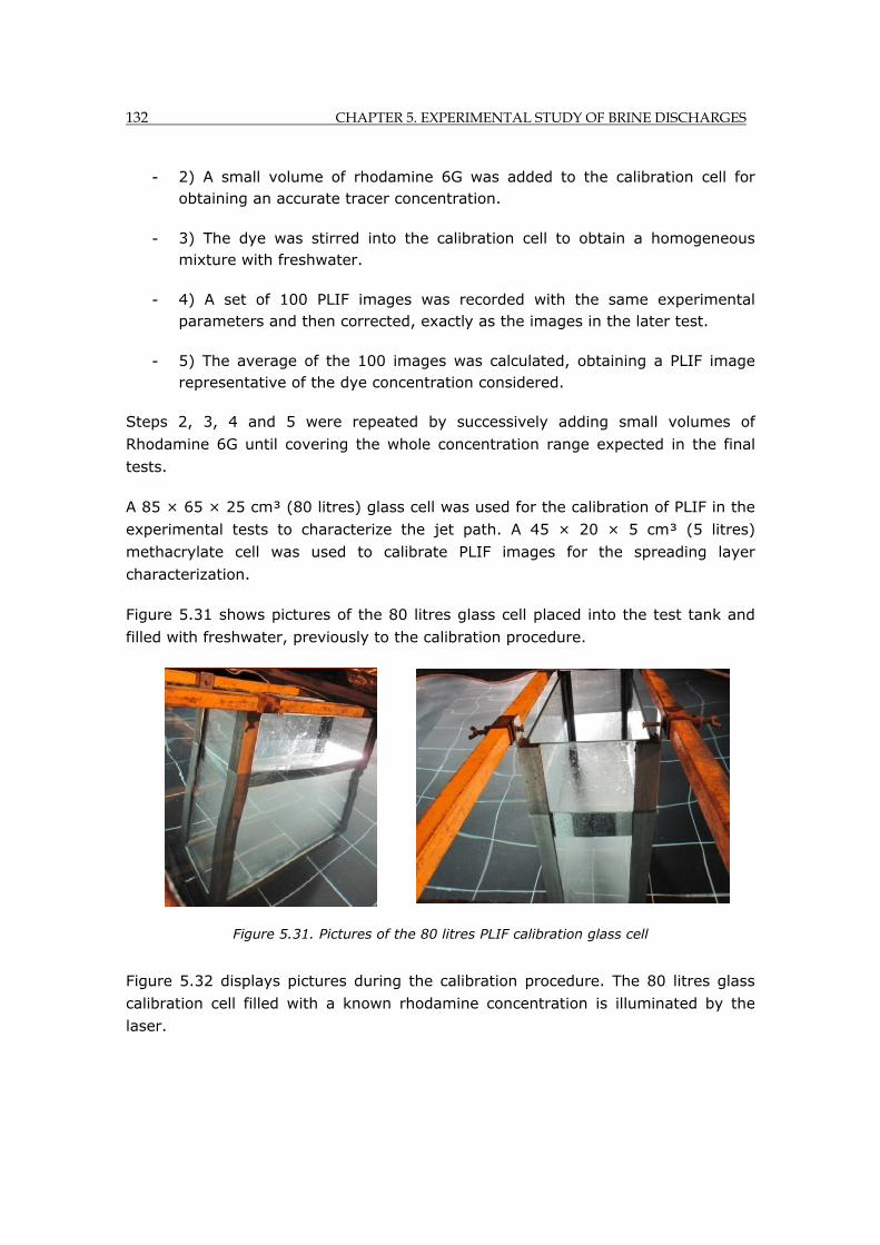
132 CHAPTER 5. EXPERIMENTAL STUDY OF BRINE DISCHARGES
- 2) A small volume of rhodamine 6G was added to the calibration cell for obtaining an accurate tracer concentration.
- 3) The dye was stirred into the calibration cell to obtain a homogeneous mixture with freshwater.
- 4) A set of 100 PLIF images was recorded with the same experimental parameters and then corrected, exactly as the images in the later test.
- 5) The average of the 100 images was calculated, obtaining a PLIF image representative of the dye concentration considered.
Steps 2, 3, 4 and 5 were repeated by successively adding small volumes of
Rhodamine 6G until covering the whole concentration range expected in the final
tests.
A 85 × 65 × 25 cm³ (80 litres) glass cell was used for the calibration of PLIF in the
experimental tests to characterize the jet path. A 45 × 20 × 5 cm³ (5 litres)
methacrylate cell was used to calibrate PLIF images for the spreading layer
characterization.
Figure 5.31 shows pictures of the 80 litres glass cell placed into the test tank and
filled with freshwater, previously to the calibration procedure.
Figure 5.31. Pictures of the 80 litres PLIF calibration glass cell
Figure 5.32 displays pictures during the calibration procedure. The 80 litres glass
calibration cell filled with a known rhodamine concentration is illuminated by the
laser.
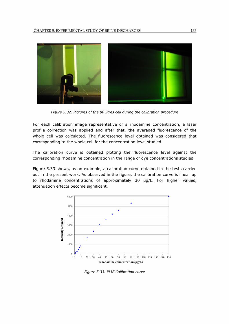
CHAPTER 5. EXPERIMENTAL STUDY OF BRINE DISCHARGES 133
Figure 5.32. Pictures of the 80 litres cell during the calibration procedure
For each calibration image representative of a rhodamine concentration, a laser
profile correction was applied and after that, the averaged fluorescence of the
whole cell was calculated. The fluorescence level obtained was considered that
corresponding to the whole cell for the concentration level studied.
The calibration curve is obtained plotting the fluorescence level against the
corresponding rhodamine concentration in the range of dye concentrations studied.
Figure 5.33 shows, as an example, a calibration curve obtained in the tests carried
out in the present work. As observed in the figure, the calibration curve is linear up
to rhodamine concentrations of approximately 30 µg/L. For higher values,
attenuation effects become significant.
Figure 5.33. PLIF Calibration curve
0
1000
2000
3000
4000
5000
6000
0 10 20 30 40 50 60 70 80 90 100 110 120 130 140 150
Inte
nsit
y (c
ount
s)
Rhodamine concentration (µg/L)
134 CHAPTER 5. EXPERIMENTAL STUDY OF BRINE DISCHARGES
In the present tests, the calibration curve corresponding to a Rhodamine 6G
concentration range from 0 µg/l to 30 µg/l has been considered to carry out the
transformation of PLIF images into concentration fields. In this range, the
calibration curve is linear, according to that observed in Figure 5.34.
Since dye tracer and salt (both contained into the brine effluent in the test) are
assumed to dilute simultaneously in the receiving water body, it is then possible to
calculate the dilution fields from the dye concentration fields.
5.5.6. Summary of PLIF parameter
Table 5.5 summarizes the PLIF parameters used in the present experiments.
Parameter Value
Fluorescent dye Rhodamine 6G
Dye concentration 250 µg/l
Images correction Geometrical correction
Laser sheet
Table 5.5. Parameters of PLIF measurements
5.6. Timing of the combined PIV-PLIF system
The timing scheme for a combined PIV-PLIF system is very important as it
coordinates the exposure time, the synchronization of the PIV and PLIF cameras
and the separation time between the laser pulses, which is crucial to obtain high
quality measurements.
Figure 5.34 shows the timing scheme for laser shooting and the exposure
procedure of the combined PIV and PLIF cameras:
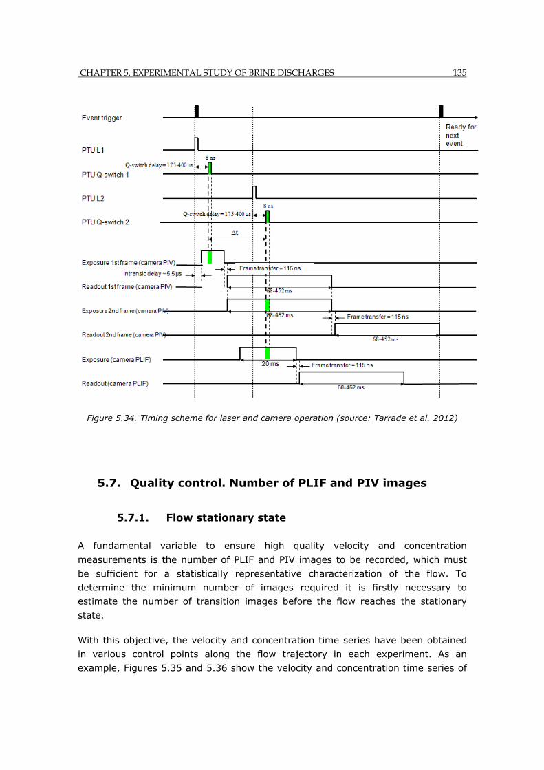
CHAPTER 5. EXPERIMENTAL STUDY OF BRINE DISCHARGES 135
Figure 5.34. Timing scheme for laser and camera operation (source: Tarrade et al. 2012)
5.7. Quality control. Number of PLIF and PIV images
5.7.1. Flow stationary state
A fundamental variable to ensure high quality velocity and concentration
measurements is the number of PLIF and PIV images to be recorded, which must
be sufficient for a statistically representative characterization of the flow. To
determine the minimum number of images required it is firstly necessary to
estimate the number of transition images before the flow reaches the stationary
state.
With this objective, the velocity and concentration time series have been obtained
in various control points along the flow trajectory in each experiment. As an
example, Figures 5.35 and 5.36 show the velocity and concentration time series of
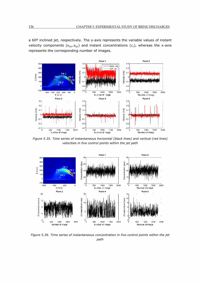
136 CHAPTER 5. EXPERIMENTAL STUDY OF BRINE DISCHARGES
a 60º inclined jet, respectively. The y-axis represents the variable values of instant
velocity components ( , ) and instant concentrations ( ), whereas the x-axis
represents the corresponding number of images.
Figure 5.35. Time series of instantaneous horizontal (black lines) and vertical (red lines) velocities in five control points within the jet path
Figure 5.36. Time series of instantaneous concentration in five control points within the jet path
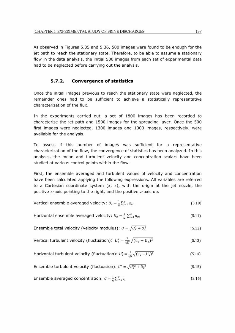
CHAPTER 5. EXPERIMENTAL STUDY OF BRINE DISCHARGES 137
As observed in Figures 5.35 and 5.36, 500 images were found to be enough for the
jet path to reach the stationary state. Therefore, to be able to assume a stationary
flow in the data analysis, the initial 500 images from each set of experimental data
had to be neglected before carrying out the analysis.
5.7.2. Convergence of statistics
Once the initial images previous to reach the stationary state were neglected, the
remainder ones had to be sufficient to achieve a statistically representative
characterization of the flux.
In the experiments carried out, a set of 1800 images has been recorded to
characterize the jet path and 1500 images for the spreading layer. Once the 500
first images were neglected, 1300 images and 1000 images, respectively, were
available for the analysis.
To assess if this number of images was sufficient for a representative
characterization of the flow, the convergence of statistics has been analyzed. In this
analysis, the mean and turbulent velocity and concentration scalars have been
studied at various control points within the flow.
First, the ensemble averaged and turbulent values of velocity and concentration
have been calculated applying the following expressions. All variables are referred
to a Cartesian coordinate system (x, z), with the origin at the jet nozzle, the
positive x-axis pointing to the right, and the positive z-axis up.
Vertical ensemble averaged velocity: ∑ (5.10)
Horizontal ensemble averaged velocity: ∑ (5.11)
Ensemble total velocity (velocity modulus): (5.12)
Vertical turbulent velocity (fluctuation): √N
u U (5.13)
Horizontal turbulent velocity (fluctuation): √N
u U (5.14)
Ensemble turbulent velocity (fluctuation): (5.15)
Ensemble averaged concentration: ∑ (5.16)
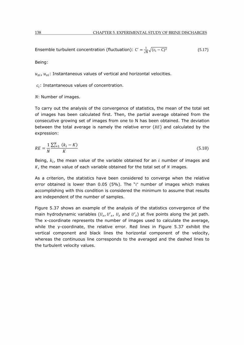
138 CHAPTER 5. EXPERIMENTAL STUDY OF BRINE DISCHARGES
Ensemble turbulent concentration (fluctuation): C√N
c C (5.17)
Being:
, : Instantaneous values of vertical and horizontal velocities.
: Instantaneous values of concentration.
: Number of images.
To carry out the analysis of the convergence of statistics, the mean of the total set
of images has been calculated first. Then, the partial average obtained from the
consecutive growing set of images from one to N has been obtained. The deviation
between the total average is namely the relative error ( ) and calculated by the
expression:
1 ∑ 5.18
Being, , the mean value of the variable obtained for an number of images and
, the mean value of each variable obtained for the total set of images.
As a criterion, the statistics have been considered to converge when the relative
error obtained is lower than 0.05 (5%). The “ " number of images which makes
accomplishing with this condition is considered the minimum to assume that results
are independent of the number of samples.
Figure 5.37 shows an example of the analysis of the statistics convergence of the
main hydrodynamic variables ( , , and ) at five points along the jet path.
The x-coordinate represents the number of images used to calculate the average,
while the y-coordinate, the relative error. Red lines in Figure 5.37 exhibit the
vertical component and black lines the horizontal component of the velocity,
whereas the continuous line corresponds to the averaged and the dashed lines to
the turbulent velocity values.
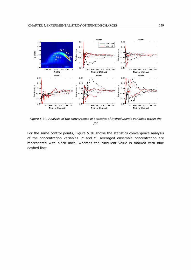
CHAPTER 5. EXPERIMENTAL STUDY OF BRINE DISCHARGES 139
Figure 5.37. Analysis of the convergence of statistics of hydrodynamic variables within the jet
For the same control points, Figure 5.38 shows the statistics convergence analysis
of the concentration variables: and . Averaged ensemble concentration are
represented with black lines, whereas the turbulent value is marked with blue
dashed lines.
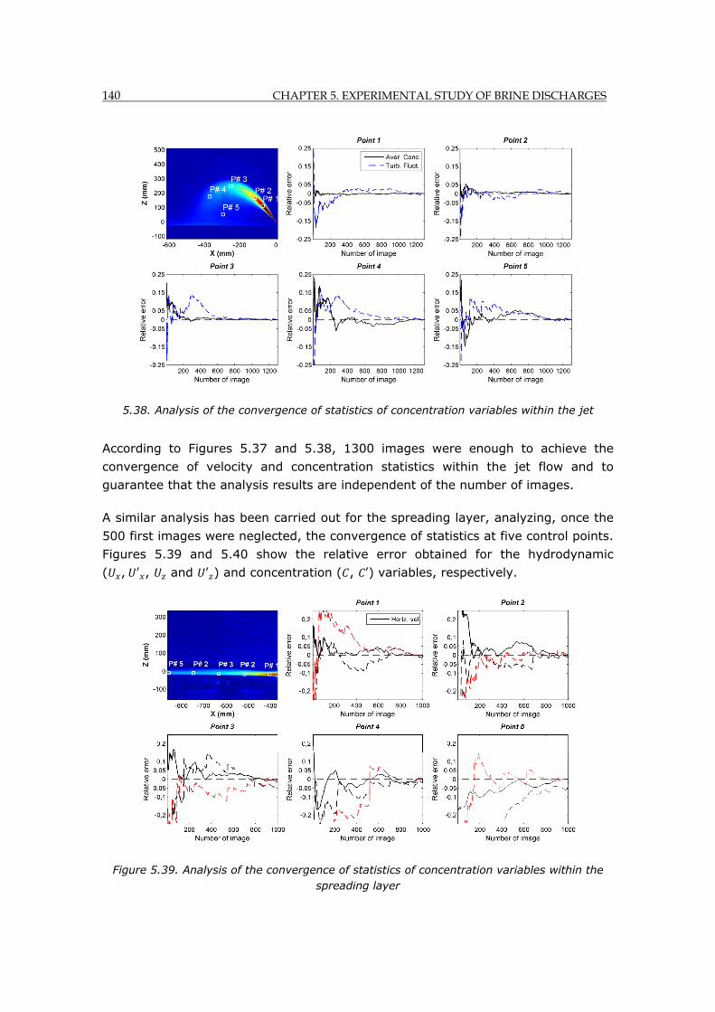
140 CHAPTER 5. EXPERIMENTAL STUDY OF BRINE DISCHARGES
5.38. Analysis of the convergence of statistics of concentration variables within the jet
According to Figures 5.37 and 5.38, 1300 images were enough to achieve the
convergence of velocity and concentration statistics within the jet flow and to
guarantee that the analysis results are independent of the number of images.
A similar analysis has been carried out for the spreading layer, analyzing, once the
500 first images were neglected, the convergence of statistics at five control points.
Figures 5.39 and 5.40 show the relative error obtained for the hydrodynamic
( , , and ) and concentration ( , ) variables, respectively.
Figure 5.39. Analysis of the convergence of statistics of concentration variables within the spreading layer
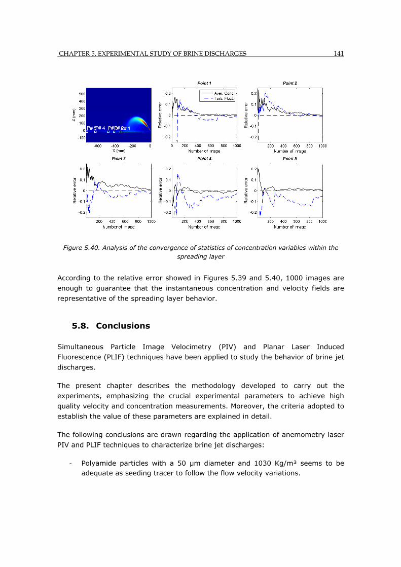
CHAPTER 5. EXPERIMENTAL STUDY OF BRINE DISCHARGES 141
Figure 5.40. Analysis of the convergence of statistics of concentration variables within the spreading layer
According to the relative error showed in Figures 5.39 and 5.40, 1000 images are
enough to guarantee that the instantaneous concentration and velocity fields are
representative of the spreading layer behavior.
5.8. Conclusions
Simultaneous Particle Image Velocimetry (PIV) and Planar Laser Induced
Fluorescence (PLIF) techniques have been applied to study the behavior of brine jet
discharges.
The present chapter describes the methodology developed to carry out the
experiments, emphasizing the crucial experimental parameters to achieve high
quality velocity and concentration measurements. Moreover, the criteria adopted to
establish the value of these parameters are explained in detail.
The following conclusions are drawn regarding the application of anemometry laser
PIV and PLIF techniques to characterize brine jet discharges:
- Polyamide particles with a 50 µm diameter and 1030 Kg/m³ seems to be adequate as seeding tracer to follow the flow velocity variations.
142 CHAPTER 5. EXPERIMENTAL STUDY OF BRINE DISCHARGES
- Due to the significant velocity gradients existing in inclined dense jets, three different separation times between the pairs of PIV images ( ) are required
to correctly characterize the velocity flow-fields. For velocities along the spreading layer, the adequate separation time ( ~30.000 ) is one order of magnitude higher than that required for velocities along the jet path ( ~5.000 ). To measure velocities at the jet zone closest to the nozzle, the separation time required ( ~300 ) is one order of magnitude lower than that needed to measure velocities along the remainder jet path ( ~5.000 ). Since only two PIV cameras were available, velocities in the zone closest to the nozzle have not been correctly measured in the present experimental tests.
- An interrogation size of 32 x 32 pixel2 was found to be satisfactory in the present tests, giving good quality velocity measurements along the jet path and the spreading layer.
- The correlation method used in the PIV images post-processing was found not to be relevant in velocity results in the present tests. Velocity results obtained applying normalized and standard cyclic FT correlation functions were quite similar. For this reason, the last one has been used in the present experiments since it is significantly less time-consuming.
- 250 µg/l was chosen as an adequate Rhodamine 6G concentration in the experiments, considering two conditions: to correctly measure concentrations in the flow zones with highest dilution and to avoid any significant laser attenuation caused by the presence of the Rhodamine 6G.
- Since free chlorine was present in Santander fresh water, sodium thiosulfate was added to the test tank freshwater to avoid any chemical reaction (photobleaching) with the Rhodamine 6G used as fluorescence tracer.
- Attenuation effects due to the water and salt have been found to be negligible in the present tests.
- For Rhodamine 6G concentrations lower than approximately 25 - 30 µg/l, attenuation effects were found to be negligible, considering the distance crossed by the laser light in the final experiments.
- For 250 µg/l brine concentration, the mixing between the effluent and the receiving fluid makes most of the flow to have a rhodamine concentration lower than 30 µg/l in the final experiments. Consequently, rhodamine attenuation can be assumed negligible, being linear the relationship between the fluorescence level and the dye concentration.

CHAPTER 5. EXPERIMENTAL STUDY OF BRINE DISCHARGES 143
- 500 images were enough for all tests to reach the stationary state. Once these images were neglected, the remaining 1300 images were found to be sufficient for achieving the convergence of hydrodynamic and concentration statistics values within the jet. Regarding the spreading layer, 1000 images were enough for a statistically representative characterization.

144 CHAPTER 5. EXPERIMENTAL STUDY OF BRINE DISCHARGES
CHAPTER 6. BRINE JET DIMENSIONAL ANALYSIS AND LONGITUDINAL PROFILE 145
Chapter 6. BRINE JET DIMENSIONAL ANALYSIS AND LONGITUDINAL PROFILE BASED ON THE EXPERIMENTAL DATA ANALYSIS
Chapter 6 BRINE JET DIMENSIONAL ANALYSIS AND LONGITUDINAL PROFILE BASED ON THE EXPERIMENTAL DATA ANALYSIS
Summary
In the previous chapter, the procedure developed to implement PIV and PLIF
techniques to the characterization of brine jet discharges is described in detail.
Once the PIV and PLIF tests were carried out, the experimental data obtained are
analyzed in the present and the following chapters in order to characterize the brine
discharge behavior in the near field region.
Various Densimetric Froude numbers (10< <40) and initial discharge angles
(15º< <75º) in the range of actual desalination plant discharges have been
considered to study their influence on the jet path behavior.
This chapter focuses on explaining the tests similarities between prototype and
tests, showing a case study and describing the criteria adopted to guarantee a fully
developed flow and a source of volume flux being negligible. The velocity and
concentration longitudinal profiles along the jet path are also characterized by the
analysis of the evolution of the main variables along these axes. Values
corresponding to different discharge angles are also compared. Applying
dimensional analysis, the empirical coefficients for the main flow variables have
been provided at singular points of the jet path. These coefficients have been
validated with experimental data found in the literature in order to assess the
reliability degree of the experimental results obtained.
146 CHAPTER 6. BRINE JET DIMENSIONAL ANALYSIS AND LONGITUDINAL PROFILE
6.1. Introduction
Experimental modeling using non-intrusive optical laser techniques PIV (Particle
Image Velocimetry) and LIF (Laser Induced Fluorescence) have been implemented
in the study of jet flows over the last two decades, especially in aeronautics, but
mainly focused on neutral or positively buoyant flows.
Research related to the characterization of negatively buoyant jets has increased
only in the last years. In Roberts et al. (1997) the near field region of a single port
60º inclined dense jet was studied using PLIF, calibrating dimensional analysis
formulas in specific points of the jet near field region. In Kikkert et al. (2007), 30º,
45º and 60º inclined dense jets were studied using PLIF and LA (Laser
Anemometry), comparing experimental results with those obtained from an
analytical numerical model. A 3DLIF system was used in Gungor et al. (2009) to
describe experimentally the behavior of vertical dense jets discharged into dynamic
environments.
More recently, an experimental research using synchronized PIV and PLIF was
carried out in Shao et al. (2010, a) to study 30º and 45º inclined dense jets. In
Shao et al. (2010, b), the same authors characterized a horizontal dense jet,
analyzing the Coanda effect and going in depth into the turbulent processes in Shao
et al. (2009). The most recent research, Oliver et al. (2013) applied PLIF to
characterize the concentration features of an inclined negatively buoyant jet, but
eliminating the influence of the bottom boundary.
In all these works, the analysis of the experimental data has focused on the
calibration of dimensional analysis formulas at specific points on the jet path.
However, the hydrodynamic and mixing processes that characterize the flow
behavior have not been deeply analyzed. The simplifying hypothesis generally
assumed by commercial models have not been evaluated either. Moreover, these
studies have been limited to jets with 30º, 45º and 60º discharge angles.
These limitations found in the literature, together with the need for a high quality
experimental database to calibrate and validate numerical models, has justified the
development of new tests. The aim of these tests being the analysis in depth of the
brine flow behavior and the understanding of the hydrodynamic and mixing
processes.
With this aim in mind, an experimental research has been carried out in the
Environmental Hydraulics Institute, covering the full range of realistic design
parameters and taking synchronized velocity and concentration measurements
along the whole near field region, including the jet path and the spreading layer.
CHAPTER 6. BRINE JET DIMENSIONAL ANALYSIS AND LONGITUDINAL PROFILE 147
The present and the following chapters focus on the analysis of the jet zone,
including the characterization of variables along longitudinal profiles and calibrating
dimensional analysis formulas of variables of interest at singular points along the
jet path, such as the maximum height, the return point and the impact point.
Variables of high interest in the discharge design, such as the jet width or
differences in the dilution ratio between the return and the impact point, not
previously reported, have been quantified and provided in the present chapter. To
assess the feasibility degree of the experimental data obtained, they have been
compared to previous works published.
6.2. Experimental test description
6.2.1. Tests and prototype similarities
Experimental modeling consists of performing laboratory test using scale physical
models, which are a model of the real case being tested, i.e.: the prototype, but
normally at a smaller scale. The model and the prototype maintain the relative
proportions (the scale factor) and they are scaled in terms of both geometry and
forces.
To guarantee the correspondence between the model and the prototype behavior,
the following conditions must be achieved:
1.) Geometric similarity exists between model and prototype if the ratio of all
corresponding dimensions in the model and prototype is equal. Dimension scales
are defined by the formulas:
For length:
6.1
For areas:
6.2
2.) Kinematic similarity refers to time and geometry. It exists between model and
prototype if the paths of moving particles are geometrically similar and if the ratio
of the particle velocities is similar. Scales include the following kinematic variables.
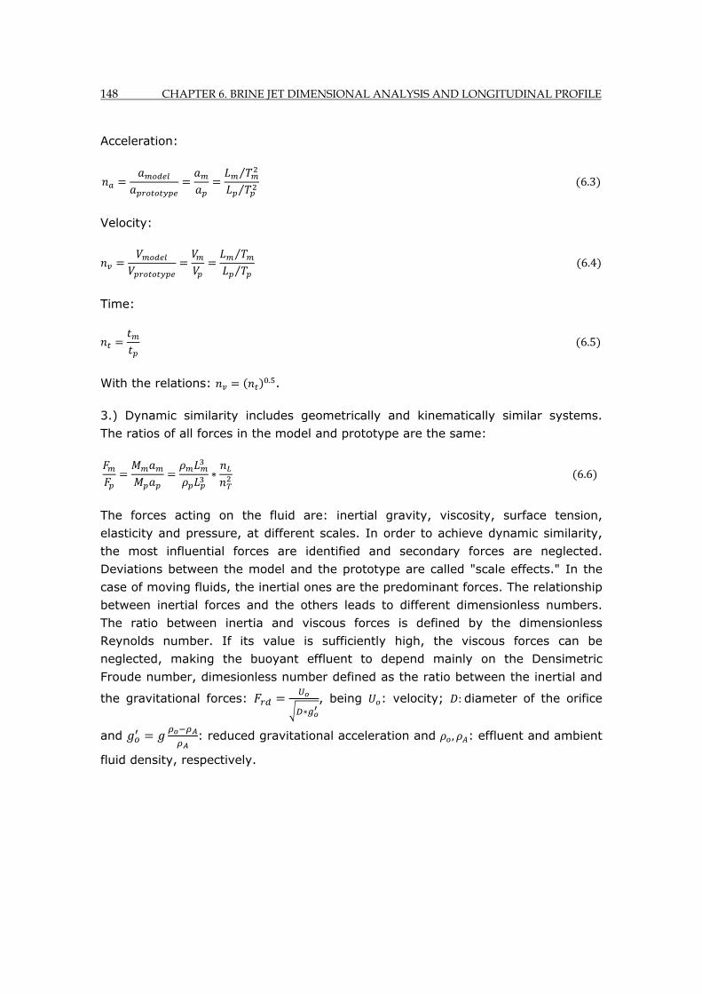
148 CHAPTER 6. BRINE JET DIMENSIONAL ANALYSIS AND LONGITUDINAL PROFILE
Acceleration:
⁄⁄
6.3
Velocity:
⁄⁄
6.4
Time:
6.5
With the relations: . .
3.) Dynamic similarity includes geometrically and kinematically similar systems.
The ratios of all forces in the model and prototype are the same:
6.6
The forces acting on the fluid are: inertial gravity, viscosity, surface tension,
elasticity and pressure, at different scales. In order to achieve dynamic similarity,
the most influential forces are identified and secondary forces are neglected.
Deviations between the model and the prototype are called "scale effects." In the
case of moving fluids, the inertial ones are the predominant forces. The relationship
between inertial forces and the others leads to different dimensionless numbers.
The ratio between inertia and viscous forces is defined by the dimensionless
Reynolds number. If its value is sufficiently high, the viscous forces can be
neglected, making the buoyant effluent to depend mainly on the Densimetric
Froude number, dimesionless number defined as the ratio between the inertial and
the gravitational forces: , being : velocity; : diameter of the orifice
and : reduced gravitational acceleration and , : effluent and ambient
fluid density, respectively.
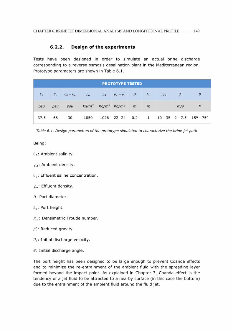
CHAPTER 6. BRINE JET DIMENSIONAL ANALYSIS AND LONGITUDINAL PROFILE 149
6.2.2. Design of the experiments
Tests have been designed in order to simulate an actual brine discharge
corresponding to a reverse osmosis desalination plant in the Mediterranean region.
Prototype parameters are shown in Table 6.1.
PROTOTYPE TESTED
psu psu psu kg/m3 Kg/m3 Kg/m³ m m m/s º
37.5 68 30 1050 1026 22- 24 0.2 1 10 - 35 2 - 7.5 15º - 75º
Table 6.1. Design parameters of the prototype simulated to characterize the brine jet path
Being:
CA: Ambient salinity.
: Ambient density.
C : Effluent saline concentration.
: Effluent density.
: Port diameter.
: Port height.
: Densimetric Froude number.
: Reduced gravity.
: Initial discharge velocity.
: Initial discharge angle.
The port height has been designed to be large enough to prevent Coanda effects and to minimize the re-entrainment of the ambient fluid with the spreading layer formed beyond the impact point. As explained in Chapter 3, Coanda effect is the tendency of a jet fluid to be attracted to a nearby surface (in this case the bottom) due to the entrainment of the ambient fluid around the fluid jet.
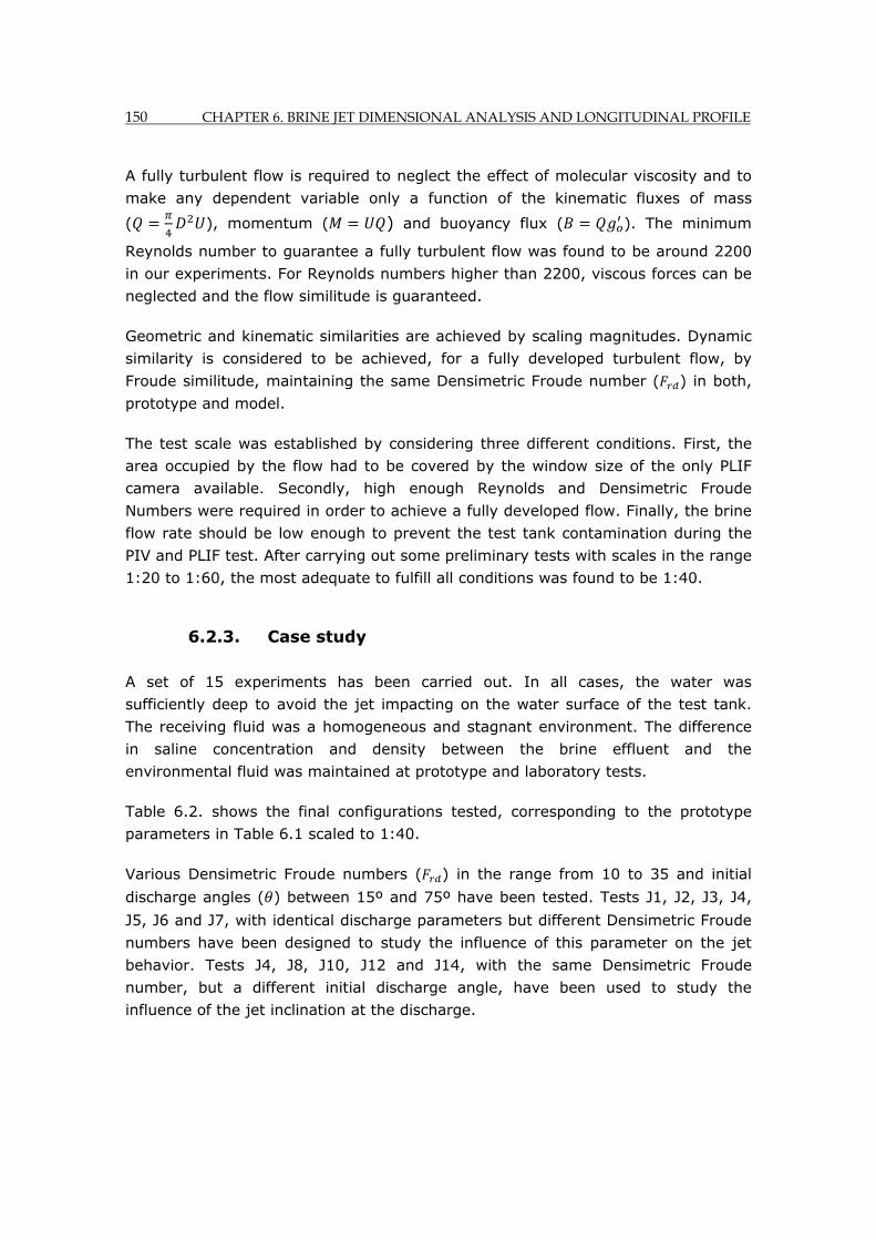
150 CHAPTER 6. BRINE JET DIMENSIONAL ANALYSIS AND LONGITUDINAL PROFILE
A fully turbulent flow is required to neglect the effect of molecular viscosity and to
make any dependent variable only a function of the kinematic fluxes of mass
( ), momentum ( ) and buoyancy flux ( ). The minimum
Reynolds number to guarantee a fully turbulent flow was found to be around 2200
in our experiments. For Reynolds numbers higher than 2200, viscous forces can be
neglected and the flow similitude is guaranteed.
Geometric and kinematic similarities are achieved by scaling magnitudes. Dynamic
similarity is considered to be achieved, for a fully developed turbulent flow, by
Froude similitude, maintaining the same Densimetric Froude number ( ) in both,
prototype and model.
The test scale was established by considering three different conditions. First, the
area occupied by the flow had to be covered by the window size of the only PLIF
camera available. Secondly, high enough Reynolds and Densimetric Froude
Numbers were required in order to achieve a fully developed flow. Finally, the brine
flow rate should be low enough to prevent the test tank contamination during the
PIV and PLIF test. After carrying out some preliminary tests with scales in the range
1:20 to 1:60, the most adequate to fulfill all conditions was found to be 1:40.
6.2.3. Case study
A set of 15 experiments has been carried out. In all cases, the water was
sufficiently deep to avoid the jet impacting on the water surface of the test tank.
The receiving fluid was a homogeneous and stagnant environment. The difference
in saline concentration and density between the brine effluent and the
environmental fluid was maintained at prototype and laboratory tests.
Table 6.2. shows the final configurations tested, corresponding to the prototype
parameters in Table 6.1 scaled to 1:40.
Various Densimetric Froude numbers ( ) in the range from 10 to 35 and initial
discharge angles ( ) between 15º and 75º have been tested. Tests J1, J2, J3, J4,
J5, J6 and J7, with identical discharge parameters but different Densimetric Froude
numbers have been designed to study the influence of this parameter on the jet
behavior. Tests J4, J8, J10, J12 and J14, with the same Densimetric Froude
number, but a different initial discharge angle, have been used to study the
influence of the jet inclination at the discharge.
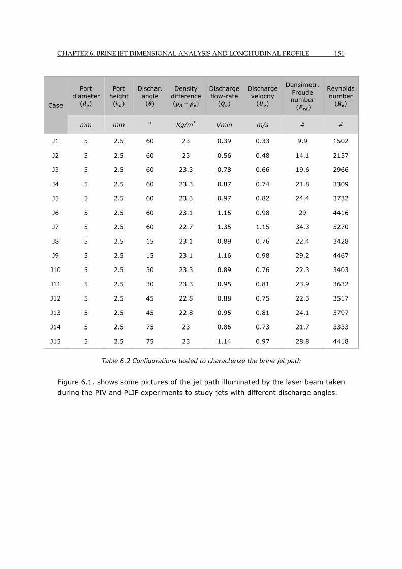
CHAPTER 6. BRINE JET DIMENSIONAL ANALYSIS AND LONGITUDINAL PROFILE 151
Case
Port diameter
( )
Port height ( )
Dischar. angle (
Density difference (
Discharge flow-rate
( )
Discharge velocity
( )
Densimetr. Froude number ( )
Reynolds number
( )
mm mm ° Kg/m3 l/min m/s # #
J1 5 2.5 60 23 0.39 0.33 9.9 1502
J2 5 2.5 60 23 0.56 0.48 14.1 2157
J3 5 2.5 60 23.3 0.78 0.66 19.6 2966
J4 5 2.5 60 23.3 0.87 0.74 21.8 3309
J5 5 2.5 60 23.3 0.97 0.82 24.4 3732
J6 5 2.5 60 23.1 1.15 0.98 29 4416
J7 5 2.5 60 22.7 1.35 1.15 34.3 5270
J8 5 2.5 15 23.1 0.89 0.76 22.4 3428
J9 5 2.5 15 23.1 1.16 0.98 29.2 4467
J10 5 2.5 30 23.3 0.89 0.76 22.3 3403
J11 5 2.5 30 23.3 0.95 0.81 23.9 3632
J12 5 2.5 45 22.8 0.88 0.75 22.3 3517
J13 5 2.5 45 22.8 0.95 0.81 24.1 3797
J14 5 2.5 75 23 0.86 0.73 21.7 3333
J15 5 2.5 75 23 1.14 0.97 28.8 4418
Table 6.2 Configurations tested to characterize the brine jet path
Figure 6.1. shows some pictures of the jet path illuminated by the laser beam taken
during the PIV and PLIF experiments to study jets with different discharge angles.
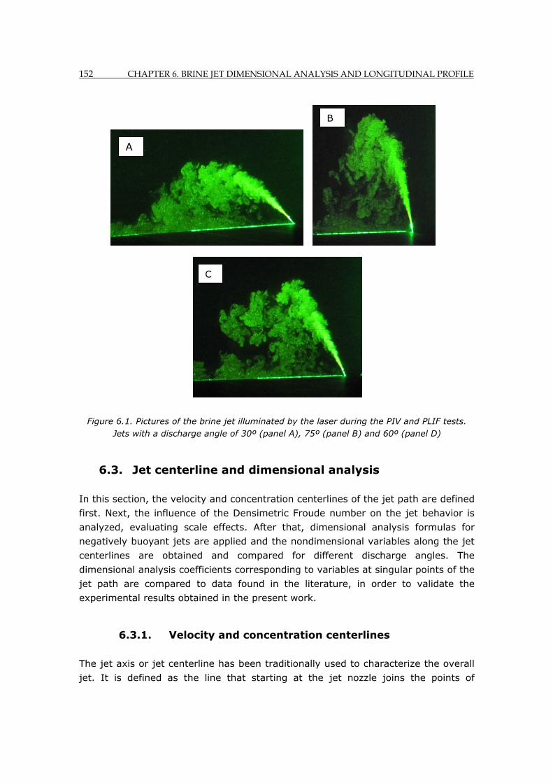
152 CHAPTER 6. BRINE JET DIMENSIONAL ANALYSIS AND LONGITUDINAL PROFILE
Figure 6.1. Pictures of the brine jet illuminated by the laser during the PIV and PLIF tests. Jets with a discharge angle of 30º (panel A), 75º (panel B) and 60º (panel D)
6.3. Jet centerline and dimensional analysis
In this section, the velocity and concentration centerlines of the jet path are defined
first. Next, the influence of the Densimetric Froude number on the jet behavior is
analyzed, evaluating scale effects. After that, dimensional analysis formulas for
negatively buoyant jets are applied and the nondimensional variables along the jet
centerlines are obtained and compared for different discharge angles. The
dimensional analysis coefficients corresponding to variables at singular points of the
jet path are compared to data found in the literature, in order to validate the
experimental results obtained in the present work.
6.3.1. Velocity and concentration centerlines
The jet axis or jet centerline has been traditionally used to characterize the overall
jet. It is defined as the line that starting at the jet nozzle joins the points of
A
C
B
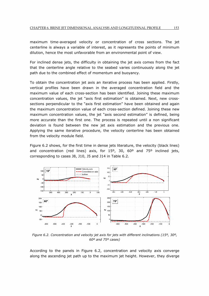
CHAPTER 6. BRINE JET DIMENSIONAL ANALYSIS AND LONGITUDINAL PROFILE 153
maximum time-averaged velocity or concentration of cross sections. The jet
centerline is always a variable of interest, as it represents the points of minimum
dilution, hence the most unfavorable from an environmental point of view.
For inclined dense jets, the difficulty in obtaining the jet axis comes from the fact
that the centerline angle relative to the seabed varies continuously along the jet
path due to the combined effect of momentum and buoyancy.
To obtain the concentration jet axis an iterative process has been applied. Firstly,
vertical profiles have been drawn in the averaged concentration field and the
maximum value of each cross-section has been identified. Joining these maximum
concentration values, the jet “axis first estimation” is obtained. Next, new cross-
sections perpendicular to the “axis first estimation” have been obtained and again
the maximum concentration value of each cross-section defined. Joining these new
maximum concentration values, the jet “axis second estimation” is defined, being
more accurate than the first one. The process is repeated until a non significant
deviation is found between the new jet axis estimation and the previous one.
Applying the same iterative procedure, the velocity centerline has been obtained
from the velocity module field.
Figure 6.2 shows, for the first time in dense jets literature, the velocity (black lines)
and concentration (red lines) axis, for 15º, 30, 60º and 75º inclined jets,
corresponding to cases J8, J10, J5 and J14 in Table 6.2.
Figure 6.2. Concentration and velocity jet axis for jets with different inclinations (15º, 30º, 60º and 75º cases)
According to the panels in Figure 6.2, concentration and velocity axis converge
along the ascending jet path up to the maximum jet height. However, they diverge
154 CHAPTER 6. BRINE JET DIMENSIONAL ANALYSIS AND LONGITUDINAL PROFILE
from some point on the descending path, and separate towards the downstream
direction. As observed in Figure 6.2, the concentration axis has always a shorter
length and it impacts the bottom sooner and with a steeper trajectory than the
velocity axis. The velocity centerline presents in all cases a smoother decay in the
downwards trajectory and at the impingement onto the bottom location maintains a
certain distance from the bottom. Similar results were found in Shao et al. (2010,
a) for 30º and 45º inclined jets.
The divergence between axis is caused by the boundary conditions for
concentrations, in which the presence of the bottom imposes a no-flux condition,
with zero vertical gradients, which leads to a flow accumulation above this
boundary, Shao et al. (2010, a). Secondly, the divergence is motivated by the
buoyancy-induced instabilities explained in detail in the following chapter. The
gravitational instabilities at the jet lower edge make the concentration axis to
descend rapidly in the downward motion, while velocity axis descends slower due to
the inertia associated to the horizontal component of momentum.
6.3.2. Jet path variables
Figure 6.3 shows a scheme of the profile view of an inclined dense jet, showing the
main variables at singular points of the jet trajectory: maximum height point (" "
subscript), return point (" " subscript), and impact point (" " subscript).
“Return” point refers to the location where the jet reaches the port height level in
its descending trajectory, whereas “impact” point corresponds to the location where
the jet centerline impacts the bottom.
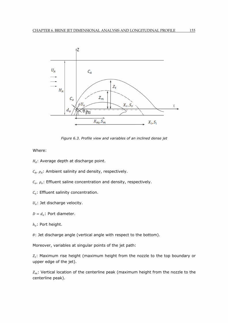
CHAPTER 6. BRINE JET DIMENSIONAL ANALYSIS AND LONGITUDINAL PROFILE 155
Figure 6.3. Profile view and variables of an inclined dense jet
Where:
: Average depth at discharge point.
, : Ambient salinity and density, respectively.
, : Effluent saline concentration and density, respectively.
: Effluent salinity concentration.
: Jet discharge velocity.
: Port diameter.
: Port height.
: Jet discharge angle (vertical angle with respect to the bottom).
Moreover, variables at singular points of the jet path:
: Maximum rise height (maximum height from the nozzle to the top boundary or
upper edge of the jet).
: Vertical location of the centerline peak (maximum height from the nozzle to the
centerline peak).

156 CHAPTER 6. BRINE JET DIMENSIONAL ANALYSIS AND LONGITUDINAL PROFILE
: Horizontal location of the centerline peak (horizontal distance reached by the
jet from the nozzle to the centerline peak location).
: Dilution at the centerline peak.
: Jet radius at the centerline peak.
: Centerline length from the nozzle to the centerline peak point.
: Horizontal location of the return point (horizontal distance reached by the jet
from the nozzle to the return point location).
: Minimum centerline dilution at the return point.
: Jet radius at the return point, defining the jet radius here as the radial distance
where concentration is 6% of concentration centerline jet.
: Centerline length from the nozzle to the return point.
: Horizontal location of the impact point (horizontal distance reached by the jet
from the nozzle to the impact point location).
: Minimum centerline dilution at the impact point.
: Densimetric Froude number, , being: : initial discharge velocity,
: reduced gravity; ; , : effluent and ambient density.
6.3.3. Influence of the Densimetric Froude number on the jet behavior
Densimetric Froude number is a dimensionless parameter, which measures the
ratio between the inertial and the gravitational force.
The effect of the Densimetric Froude number ( ) on the jet behavior is analyzed in
this section in order to study the scale effects and to determine the minimum value
of this parameter required to neglect the effect of the source volume flux.
Cases J1, J2, J3, J4, J5, J6 and J7 in Table 6.2 have been considered since they
have identical design parameters, but different Densimetric Froude numbers,
varying in the range from 10 to 35.
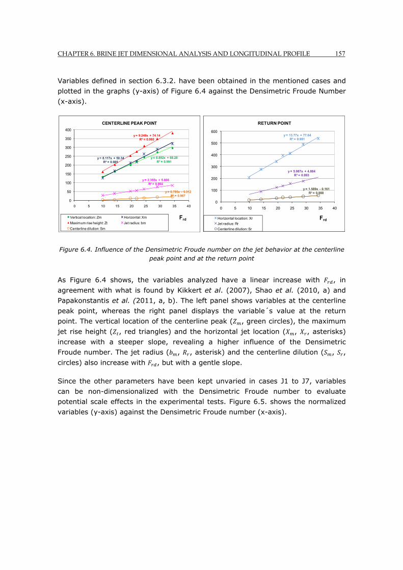
CHAPTER 6. BRINE JET DIMENSIONAL ANALYSIS AND LONGITUDINAL PROFILE 157
Variables defined in section 6.3.2. have been obtained in the mentioned cases and
plotted in the graphs (y-axis) of Figure 6.4 against the Densimetric Froude Number
(x-axis).
Figure 6.4. Influence of the Densimetric Froude number on the jet behavior at the centerline peak point and at the return point
As Figure 6.4 shows, the variables analyzed have a linear increase with , in
agreement with what is found by Kikkert et al. (2007), Shao et al. (2010, a) and
Papakonstantis et al. (2011, a, b). The left panel shows variables at the centerline
peak point, whereas the right panel displays the variable´s value at the return
point. The vertical location of the centerline peak ( , green circles), the maximum
jet rise height ( , red triangles) and the horizontal jet location ( , , asterisks)
increase with a steeper slope, revealing a higher influence of the Densimetric
Froude number. The jet radius ( , , asterisk) and the centerline dilution ( , ,
circles) also increase with , but with a gentle slope.
Since the other parameters have been kept unvaried in cases J1 to J7, variables
can be non-dimensionalized with the Densimetric Froude number to evaluate
potential scale effects in the experimental tests. Figure 6.5. shows the normalized
variables (y-axis) against the Densimetric Froude number (x-axis).
y = 6.892x + 68.28R² = 0.991
y = 8.117x + 50.34R² = 0.985
y = 9.248x + 74.14R² = 0.993
y = 2.355x + 5.866R² = 0.992
y = 0.785x - 5.312R² = 0.967
0
50
100
150
200
250
300
350
400
0 5 10 15 20 25 30 35 40
Frd
CENTERLINE PEAK POINT
Vertical location: Zm Horizontal: Xm
Maximum rise height: Zt Jet radius: bm
Centerline dilution: Sm
y = 13.77x + 77.64R² = 0.991
y = 5.987x + 4.884R² = 0.993
y = 1.589x - 0.161R² = 0.988
0
100
200
300
400
500
600
0 5 10 15 20 25 30 35 40
Frd
RETURN POINT
Horizontal location: Xr
Jet radius: Rr
Centerline dilution: Sr
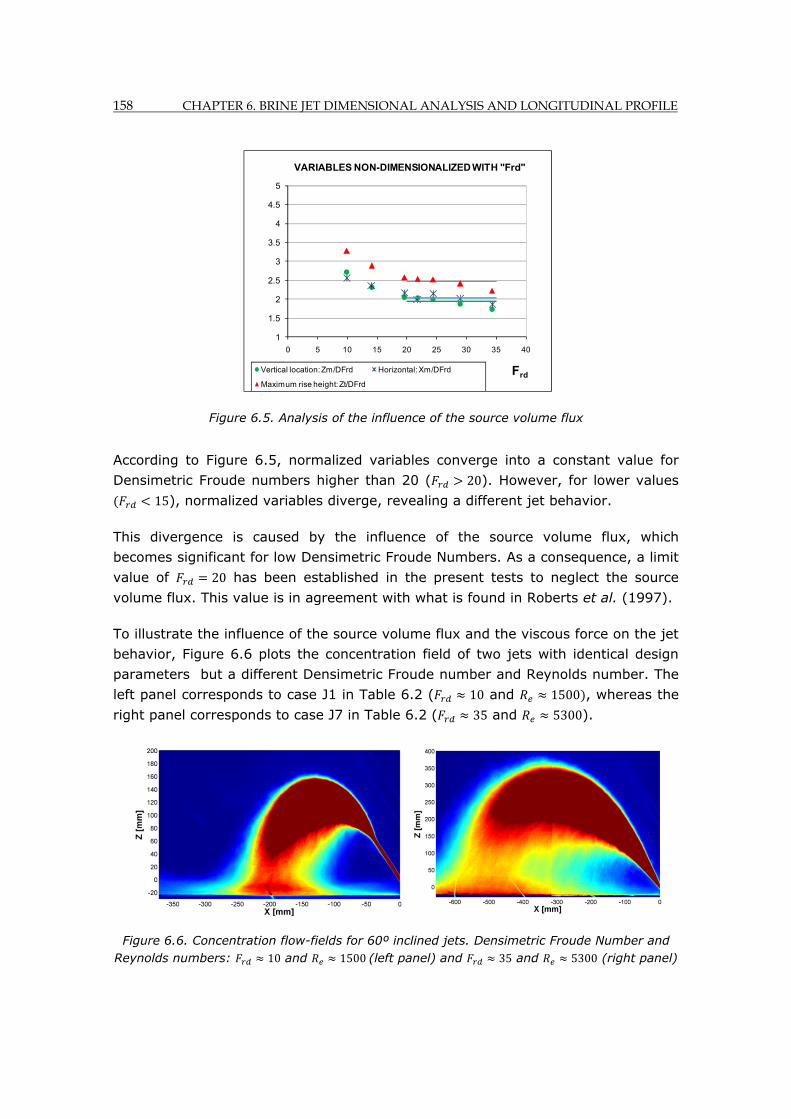
158 CHAPTER 6. BRINE JET DIMENSIONAL ANALYSIS AND LONGITUDINAL PROFILE
Figure 6.5. Analysis of the influence of the source volume flux
According to Figure 6.5, normalized variables converge into a constant value for
Densimetric Froude numbers higher than 20 ( 20). However, for lower values
15), normalized variables diverge, revealing a different jet behavior.
This divergence is caused by the influence of the source volume flux, which
becomes significant for low Densimetric Froude Numbers. As a consequence, a limit
value of 20 has been established in the present tests to neglect the source
volume flux. This value is in agreement with what is found in Roberts et al. (1997).
To illustrate the influence of the source volume flux and the viscous force on the jet
behavior, Figure 6.6 plots the concentration field of two jets with identical design
parameters but a different Densimetric Froude number and Reynolds number. The
left panel corresponds to case J1 in Table 6.2 ( 10 and 1500 , whereas the
right panel corresponds to case J7 in Table 6.2 ( 35 and 5300).
Figure 6.6. Concentration flow-fields for 60º inclined jets. Densimetric Froude Number and Reynolds numbers: 10 and 1500 (left panel) and 35 and 5300 (right panel)
1
1.5
2
2.5
3
3.5
4
4.5
5
0 5 10 15 20 25 30 35 40
Frd
VARIABLES NON-DIMENSIONALIZED WITH "Frd"
Vertical location: Zm/DFrd Horizontal: Xm/DFrd
Maximum rise height: Zt/DFrd
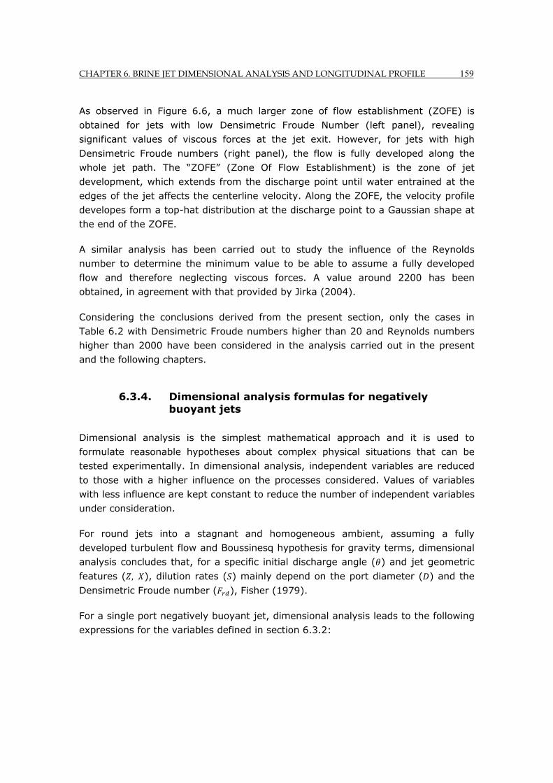
CHAPTER 6. BRINE JET DIMENSIONAL ANALYSIS AND LONGITUDINAL PROFILE 159
As observed in Figure 6.6, a much larger zone of flow establishment (ZOFE) is
obtained for jets with low Densimetric Froude Number (left panel), revealing
significant values of viscous forces at the jet exit. However, for jets with high
Densimetric Froude numbers (right panel), the flow is fully developed along the
whole jet path. The “ZOFE” (Zone Of Flow Establishment) is the zone of jet
development, which extends from the discharge point until water entrained at the
edges of the jet affects the centerline velocity. Along the ZOFE, the velocity profile
developes form a top-hat distribution at the discharge point to a Gaussian shape at
the end of the ZOFE.
A similar analysis has been carried out to study the influence of the Reynolds
number to determine the minimum value to be able to assume a fully developed
flow and therefore neglecting viscous forces. A value around 2200 has been
obtained, in agreement with that provided by Jirka (2004).
Considering the conclusions derived from the present section, only the cases in
Table 6.2 with Densimetric Froude numbers higher than 20 and Reynolds numbers
higher than 2000 have been considered in the analysis carried out in the present
and the following chapters.
6.3.4. Dimensional analysis formulas for negatively buoyant jets
Dimensional analysis is the simplest mathematical approach and it is used to
formulate reasonable hypotheses about complex physical situations that can be
tested experimentally. In dimensional analysis, independent variables are reduced
to those with a higher influence on the processes considered. Values of variables
with less influence are kept constant to reduce the number of independent variables
under consideration.
For round jets into a stagnant and homogeneous ambient, assuming a fully
developed turbulent flow and Boussinesq hypothesis for gravity terms, dimensional
analysis concludes that, for a specific initial discharge angle ( ) and jet geometric
features ( , ), dilution rates ( ) mainly depend on the port diameter ( ) and the
Densimetric Froude number ( ), Fisher (1979).
For a single port negatively buoyant jet, dimensional analysis leads to the following
expressions for the variables defined in section 6.3.2:
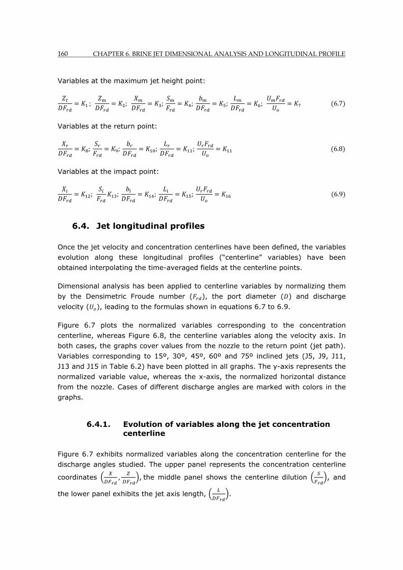
160 CHAPTER 6. BRINE JET DIMENSIONAL ANALYSIS AND LONGITUDINAL PROFILE
Variables at the maximum jet height point:
; ; ; ; ; ; 6.7
Variables at the return point:
; ; ; ; 6.8
Variables at the impact point:
; ; ; ; 6.9
6.4. Jet longitudinal profiles
Once the jet velocity and concentration centerlines have been defined, the variables
evolution along these longitudinal profiles (“centerline” variables) have been
obtained interpolating the time-averaged fields at the centerline points.
Dimensional analysis has been applied to centerline variables by normalizing them
by the Densimetric Froude number ( ), the port diameter ( ) and discharge
velocity ( ), leading to the formulas shown in equations 6.7 to 6.9.
Figure 6.7 plots the normalized variables corresponding to the concentration
centerline, whereas Figure 6.8, the centerline variables along the velocity axis. In
both cases, the graphs cover values from the nozzle to the return point (jet path).
Variables corresponding to 15º, 30º, 45º, 60º and 75º inclined jets (J5, J9, J11,
J13 and J15 in Table 6.2) have been plotted in all graphs. The y-axis represents the
normalized variable value, whereas the x-axis, the normalized horizontal distance
from the nozzle. Cases of different discharge angles are marked with colors in the
graphs.
6.4.1. Evolution of variables along the jet concentration centerline
Figure 6.7 exhibits normalized variables along the concentration centerline for the
discharge angles studied. The upper panel represents the concentration centerline
coordinates ,
, the middle panel shows the centerline dilution , and
the lower panel exhibits the jet axis length, .
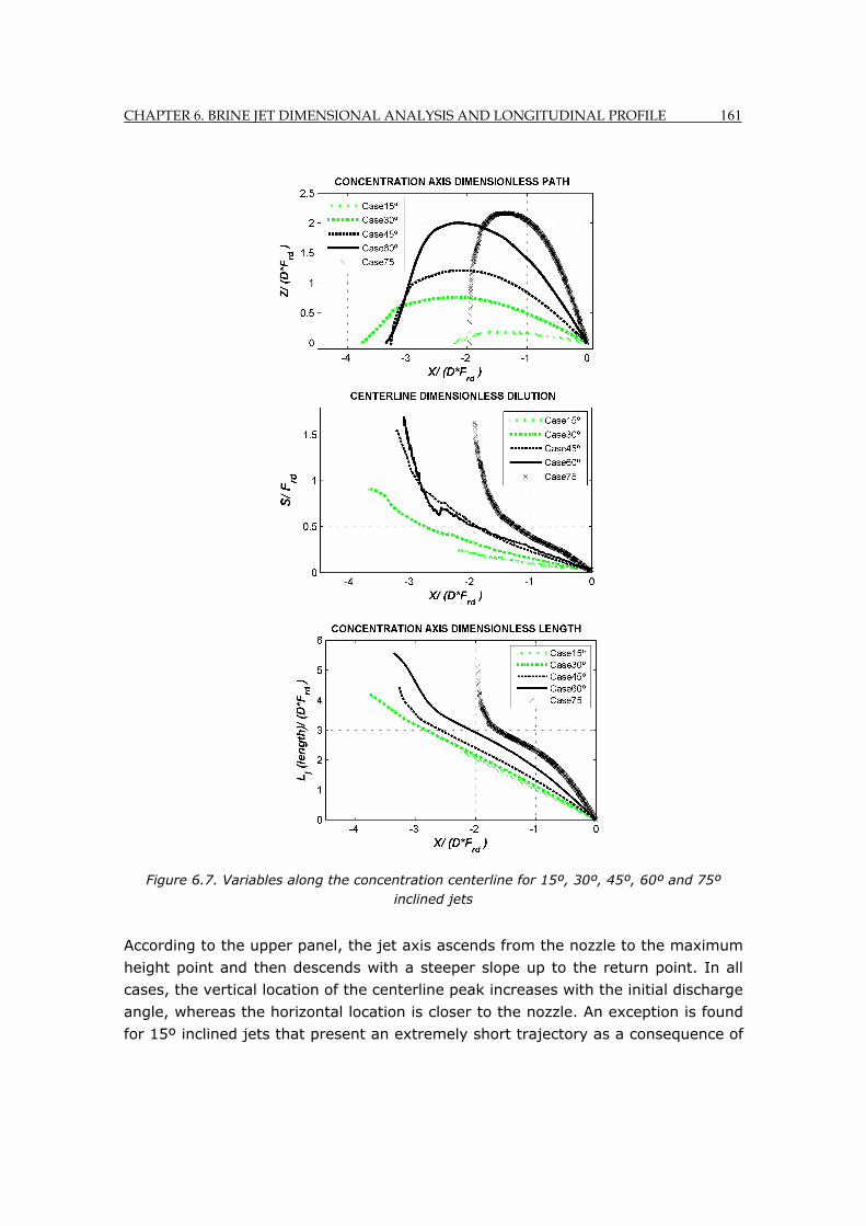
CHAPTER 6. BRINE JET DIMENSIONAL ANALYSIS AND LONGITUDINAL PROFILE 161
Figure 6.7. Variables along the concentration centerline for 15º, 30º, 45º, 60º and 75º inclined jets
According to the upper panel, the jet axis ascends from the nozzle to the maximum
height point and then descends with a steeper slope up to the return point. In all
cases, the vertical location of the centerline peak increases with the initial discharge
angle, whereas the horizontal location is closer to the nozzle. An exception is found
for 15º inclined jets that present an extremely short trajectory as a consequence of
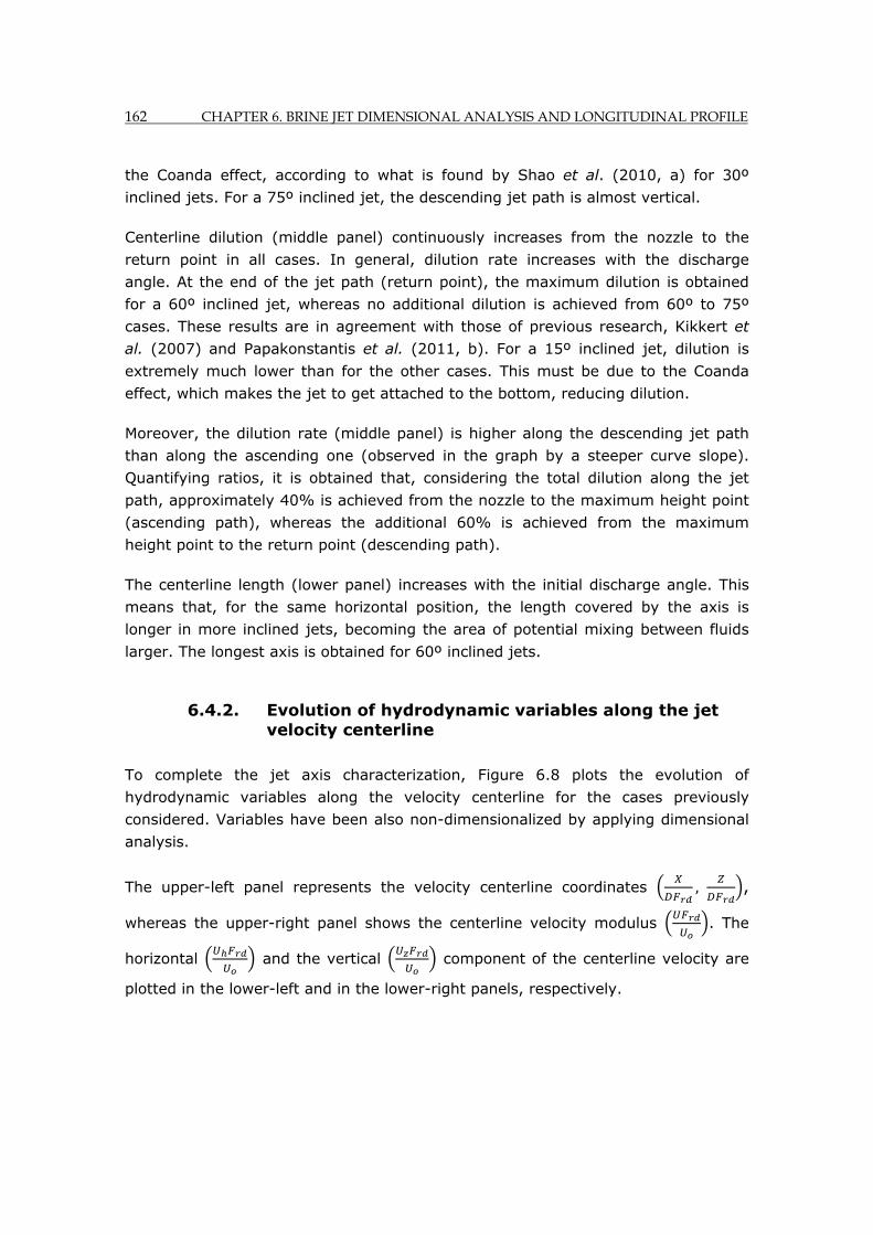
162 CHAPTER 6. BRINE JET DIMENSIONAL ANALYSIS AND LONGITUDINAL PROFILE
the Coanda effect, according to what is found by Shao et al. (2010, a) for 30º
inclined jets. For a 75º inclined jet, the descending jet path is almost vertical.
Centerline dilution (middle panel) continuously increases from the nozzle to the
return point in all cases. In general, dilution rate increases with the discharge
angle. At the end of the jet path (return point), the maximum dilution is obtained
for a 60º inclined jet, whereas no additional dilution is achieved from 60º to 75º
cases. These results are in agreement with those of previous research, Kikkert et
al. (2007) and Papakonstantis et al. (2011, b). For a 15º inclined jet, dilution is
extremely much lower than for the other cases. This must be due to the Coanda
effect, which makes the jet to get attached to the bottom, reducing dilution.
Moreover, the dilution rate (middle panel) is higher along the descending jet path
than along the ascending one (observed in the graph by a steeper curve slope).
Quantifying ratios, it is obtained that, considering the total dilution along the jet
path, approximately 40% is achieved from the nozzle to the maximum height point
(ascending path), whereas the additional 60% is achieved from the maximum
height point to the return point (descending path).
The centerline length (lower panel) increases with the initial discharge angle. This
means that, for the same horizontal position, the length covered by the axis is
longer in more inclined jets, becoming the area of potential mixing between fluids
larger. The longest axis is obtained for 60º inclined jets.
6.4.2. Evolution of hydrodynamic variables along the jet velocity centerline
To complete the jet axis characterization, Figure 6.8 plots the evolution of
hydrodynamic variables along the velocity centerline for the cases previously
considered. Variables have been also non-dimensionalized by applying dimensional
analysis.
The upper-left panel represents the velocity centerline coordinates , ,
whereas the upper-right panel shows the centerline velocity modulus . The
horizontal and the vertical component of the centerline velocity are
plotted in the lower-left and in the lower-right panels, respectively.
CHAPTER 6. BRINE JET DIMENSIONAL ANALYSIS AND LONGITUDINAL PROFILE 163
Figure 6.8. Hydrodynamic variables along the velocity centerline for 15º, 30º, 45º, 60º and 75º inclined jets
The velocity centerline (upper-left panel) presents a similar trajectory to that of the
concentration axis. Again, the vertical location of the centerline peak increases with
the initial discharge angle, while the horizontal location decreases. Contrary to the
concentration centerline, the velocity axis descends smoothly.
Centerline velocity modulus (upper-right panel) continuously decreases from the
nozzle to the return point. In the present tests, velocities have not been correctly
measured in the zone close to the nozzle, since a much lower time between pulses
( ) would have been required (section 5.4.4). For this reason, velocity values at
this zone have been removed from the graph.
The horizontal component of the centerline velocity (lower-left panel) diminishes
along the jet path, being the momentum damping more rapid during the ascending
path. For highly inclined jets (75º case), the horizontal velocity at the downward
path is close to zero, evidencing an almost vertical descending path. The velocity
modulus (upper-right panel) and its horizontal component (lower-left panel) show
wiggles at the end of the jet path, which must be caused by the presence of large
stable structures that will be described in the following chapter.
164 CHAPTER 6. BRINE JET DIMENSIONAL ANALYSIS AND LONGITUDINAL PROFILE
The vertical component of velocity (lower-right panel) is observed to decrease from
the nozzle to the maximum centerline peak due to the combined action of friction
and gravity. At the centerline peak, the vertical velocity is zero in all cases, as
shown on the panel. Beyond this point, the jet descends (negative values of the
vertical component of velocity) due to the gravitational force.
Comparing the hydrodynamic centerline variables from cases with different
discharge angles, it is observed that flow is predominantly horizontal for 15º, 30º
and 45º inclined jets, whereas it is predominantly vertical for 60º and 75º
inclinations.
Relating concentration and velocity centerline variables, it seems that dilution
depends on the jet centerline length and on the vertical component of the velocity.
For cases with the largest centerline length and the highest vertical component, the
maximum dilution rate is achieved. The centerline length represents the available
distance for the effluent to mix with the surrounding fluid. Furthermore, the vertical
component of velocity seems to be related to effective mixing processes between
the jet flow and the receiving fluid. According to this, 60º and 75º inclined jets,
having the largest trajectory length and the highest vertical velocity, achieve the
highest dilution rates along the jet path.
6.4.3. Experimental coefficients at singular points
From the nondimensional velocity and concentration centerline variables for each
case in Table 6.2, the calibration coefficients ( , in equations 6.7, 6.8 and 6.9)
have been obtained. These coefficients characterize the jet at singular points of its
trajectory.
Figure 6.9 plots these calibration coefficients obtained for all cases in Table 6.2,
except for J1 and J2, which have not been considered since they have very low
values of the Densimetric Froude Number. The left panel displays the coefficients
for the maximum rise height and the horizontal location of the return point,
obtained from the concentration centerline. The right panel shows the coefficients
for dilution formulas at the centerline peak and at the return point. The y-axis
represents the nondimensional value, whereas the x-axis, the corresponding
discharge angle.
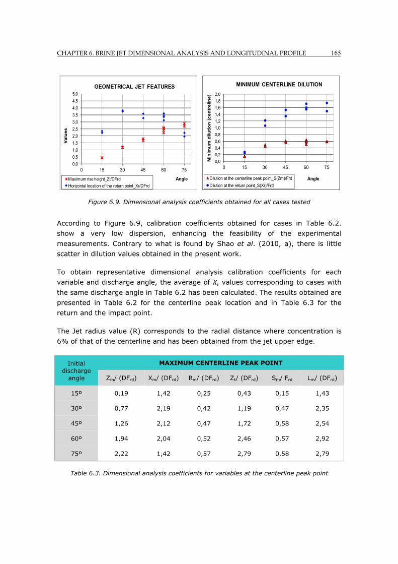
CHAPTER 6. BRINE JET DIMENSIONAL ANALYSIS AND LONGITUDINAL PROFILE 165
Figure 6.9. Dimensional analysis coefficients obtained for all cases tested
According to Figure 6.9, calibration coefficients obtained for cases in Table 6.2.
show a very low dispersion, enhancing the feasibility of the experimental
measurements. Contrary to what is found by Shao et al. (2010, a), there is little
scatter in dilution values obtained in the present work.
To obtain representative dimensional analysis calibration coefficients for each
variable and discharge angle, the average of values corresponding to cases with
the same discharge angle in Table 6.2 has been calculated. The results obtained are
presented in Table 6.2 for the centerline peak location and in Table 6.3 for the
return and the impact point.
The Jet radius value (R) corresponds to the radial distance where concentration is
6% of that of the centerline and has been obtained from the jet upper edge.
Initial discharge
angle
MAXIMUM CENTERLINE PEAK POINT
Zm/ (DFrd) Xm/ (DFrd) Rm/ (DFrd) Zt/ (DFrd) Sm/ Frd Lm/ (DFrd)
15º 0,19 1,42 0,25 0,43 0,15 1,43
30º 0,77 2,19 0,42 1,19 0,47 2,35
45º 1,26 2,12 0,47 1,72 0,58 2,54
60º 1,94 2,04 0,52 2,46 0,57 2,92
75º 2,22 1,42 0,57 2,79 0,58 2,79
Table 6.3. Dimensional analysis coefficients for variables at the centerline peak point
0,0
0,5
1,0
1,5
2,0
2,5
3,0
3,5
4,0
4,5
5,0
0 15 30 45 60 75
Va
lue
s
Angle
GEOMETRICAL JET FEATURES
Maximum rise height_Zt/DFrd
Horizontal location of the return point_Xr/DFrd
0,0
0,2
0,4
0,6
0,8
1,0
1,2
1,4
1,6
1,8
2,0
0 15 30 45 60 75
Min
imu
m d
iluti
on
(c
en
tre
lin
e)
Angle
MINIMUM CENTERLINE DILUTION
Dilution at the centerline peak point_S(Zm)/Frd
Dilution at the return point_S(Xr)/Frd
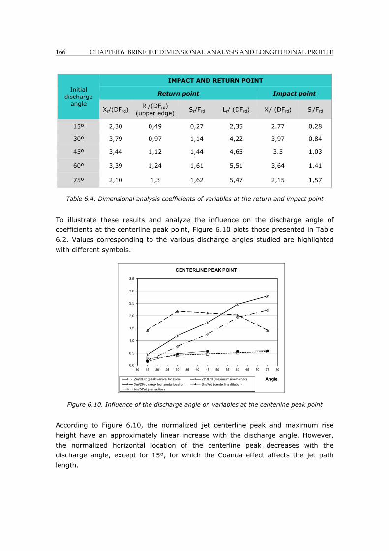
166 CHAPTER 6. BRINE JET DIMENSIONAL ANALYSIS AND LONGITUDINAL PROFILE
Initial discharge
angle
IMPACT AND RETURN POINT
Return point Impact point
Xr/(DFrd) Rr/(DFrd)
(upper edge) Sr/Frd Lr/ (DFrd) Xi/ (DFrd) Si/Frd
15º 2,30 0,49 0,27 2,35 2.77 0,28
30º 3,79 0,97 1,14 4,22 3,97 0,84
45º 3,44 1,12 1,44 4,65 3.5 1,03
60º 3,39 1,24 1,61 5,51 3,64 1.41
75º 2,10 1,3 1,62 5,47 2,15 1,57
Table 6.4. Dimensional analysis coefficients of variables at the return and impact point
To illustrate these results and analyze the influence on the discharge angle of
coefficients at the centerline peak point, Figure 6.10 plots those presented in Table
6.2. Values corresponding to the various discharge angles studied are highlighted
with different symbols.
Figure 6.10. Influence of the discharge angle on variables at the centerline peak point
According to Figure 6.10, the normalized jet centerline peak and maximum rise
height have an approximately linear increase with the discharge angle. However,
the normalized horizontal location of the centerline peak decreases with the
discharge angle, except for 15º, for which the Coanda effect affects the jet path
length.
0,0
0,5
1,0
1,5
2,0
2,5
3,0
3,5
10 15 20 25 30 35 40 45 50 55 60 65 70 75 80
Angle
CENTERLINE PEAK POINT
Zm/DFrd(peak vertical location) Zt/DFrd (maximum rise height)
Xm/DFrd (peak horizontal location) Sm/Frd (centerline dilution)
bm/DFrd (Jet radius)
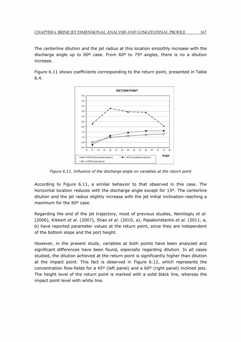
CHAPTER 6. BRINE JET DIMENSIONAL ANALYSIS AND LONGITUDINAL PROFILE 167
The centerline dilution and the jet radius at this location smoothly increase with the
discharge angle up to 60º case. From 60º to 75º angles, there is no a dilution
increase.
Figure 6.11 shows coefficients corresponding to the return point, presented in Table
6.4.
Figure 6.11. Influence of the discharge angle on variables at the return point
According to Figure 6.11, a similar behavior to that observed in this case. The
horizontal location reduces with the discharge angle except for 15º. The centerline
dilution and the jet radius slightly increase with the jet initial inclination reaching a
maximum for the 60º case.
Regarding the end of the jet trajectory, most of previous studies, Nemlioglu et al.
(2006), Kikkert et al. (2007), Shao et al. (2010, a), Papakonstantis et al. (2011, a,
b) have reported parameter values at the return point, since they are independent
of the bottom slope and the port height.
However, in the present study, variables at both points have been analyzed and
significant differences have been found, especially regarding dilution. In all cases
studied, the dilution achieved at the return point is significantly higher than dilution
at the impact point. This fact is observed in Figure 6.12, which represents the
concentration flow-fields for a 45º (left panel) and a 60º (right panel) inclined jets.
The height level of the return point is marked with a solid black line, whereas the
impact point level with white line.
0,0
0,5
1,0
1,5
2,0
2,5
3,0
3,5
4,0
4,5
5,0
10 15 20 25 30 35 40 45 50 55 60 65 70 75 80
Angle
RETURN POINT
Xr/DFrd (horizontal location) Sr/Frd (centerline dilution)
br/DFrd (Jet radius)
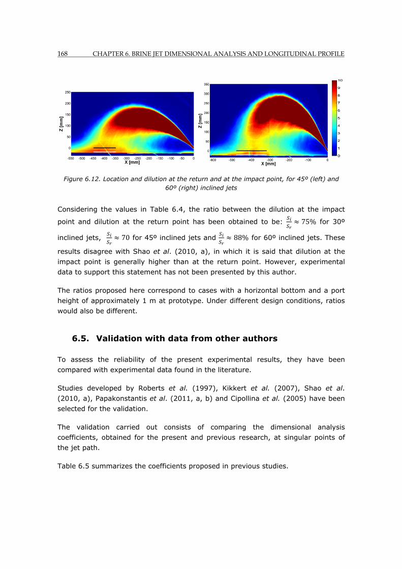
168 CHAPTER 6. BRINE JET DIMENSIONAL ANALYSIS AND LONGITUDINAL PROFILE
Figure 6.12. Location and dilution at the return and at the impact point, for 45º (left) and 60º (right) inclined jets
Considering the values in Table 6.4, the ratio between the dilution at the impact
point and dilution at the return point has been obtained to be: 75% for 30º
inclined jets, 70 for 45º inclined jets and 88% for 60º inclined jets. These
results disagree with Shao et al. (2010, a), in which it is said that dilution at the
impact point is generally higher than at the return point. However, experimental
data to support this statement has not been presented by this author.
The ratios proposed here correspond to cases with a horizontal bottom and a port
height of approximately 1 m at prototype. Under different design conditions, ratios
would also be different.
6.5. Validation with data from other authors
To assess the reliability of the present experimental results, they have been
compared with experimental data found in the literature.
Studies developed by Roberts et al. (1997), Kikkert et al. (2007), Shao et al.
(2010, a), Papakonstantis et al. (2011, a, b) and Cipollina et al. (2005) have been
selected for the validation.
The validation carried out consists of comparing the dimensional analysis
coefficients, obtained for the present and previous research, at singular points of
the jet path.
Table 6.5 summarizes the coefficients proposed in previous studies.
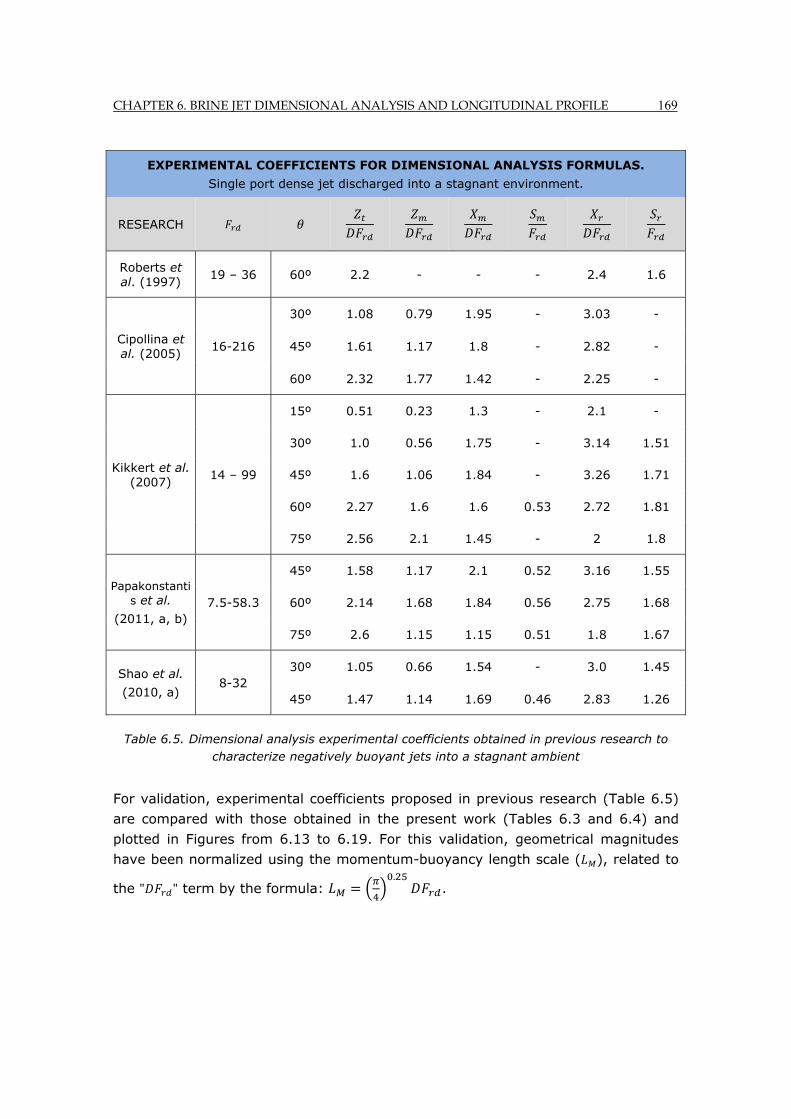
CHAPTER 6. BRINE JET DIMENSIONAL ANALYSIS AND LONGITUDINAL PROFILE 169
Table 6.5. Dimensional analysis experimental coefficients obtained in previous research to characterize negatively buoyant jets into a stagnant ambient
For validation, experimental coefficients proposed in previous research (Table 6.5)
are compared with those obtained in the present work (Tables 6.3 and 6.4) and
plotted in Figures from 6.13 to 6.19. For this validation, geometrical magnitudes
have been normalized using the momentum-buoyancy length scale ( ), related to
the " " term by the formula: .
.
EXPERIMENTAL COEFFICIENTS FOR DIMENSIONAL ANALYSIS FORMULAS.
Single port dense jet discharged into a stagnant environment.
RESEARCH
Roberts et al. (1997)
19 – 36 60º 2.2 - - - 2.4 1.6
Cipollina et al. (2005)
16-216
30º 1.08 0.79 1.95 - 3.03 -
45º 1.61 1.17 1.8 - 2.82 -
60º 2.32 1.77 1.42 - 2.25 -
Kikkert et al. (2007)
14 – 99
15º 0.51 0.23 1.3 - 2.1 -
30º 1.0 0.56 1.75 - 3.14 1.51
45º 1.6 1.06 1.84 - 3.26 1.71
60º 2.27 1.6 1.6 0.53 2.72 1.81
75º 2.56 2.1 1.45 - 2 1.8
Papakonstantis et al.
(2011, a, b) 7.5-58.3
45º 1.58 1.17 2.1 0.52 3.16 1.55
60º 2.14 1.68 1.84 0.56 2.75 1.68
75º 2.6 1.15 1.15 0.51 1.8 1.67
Shao et al.
(2010, a) 8-32
30º 1.05 0.66 1.54 - 3.0 1.45
45º 1.47 1.14 1.69 0.46 2.83 1.26
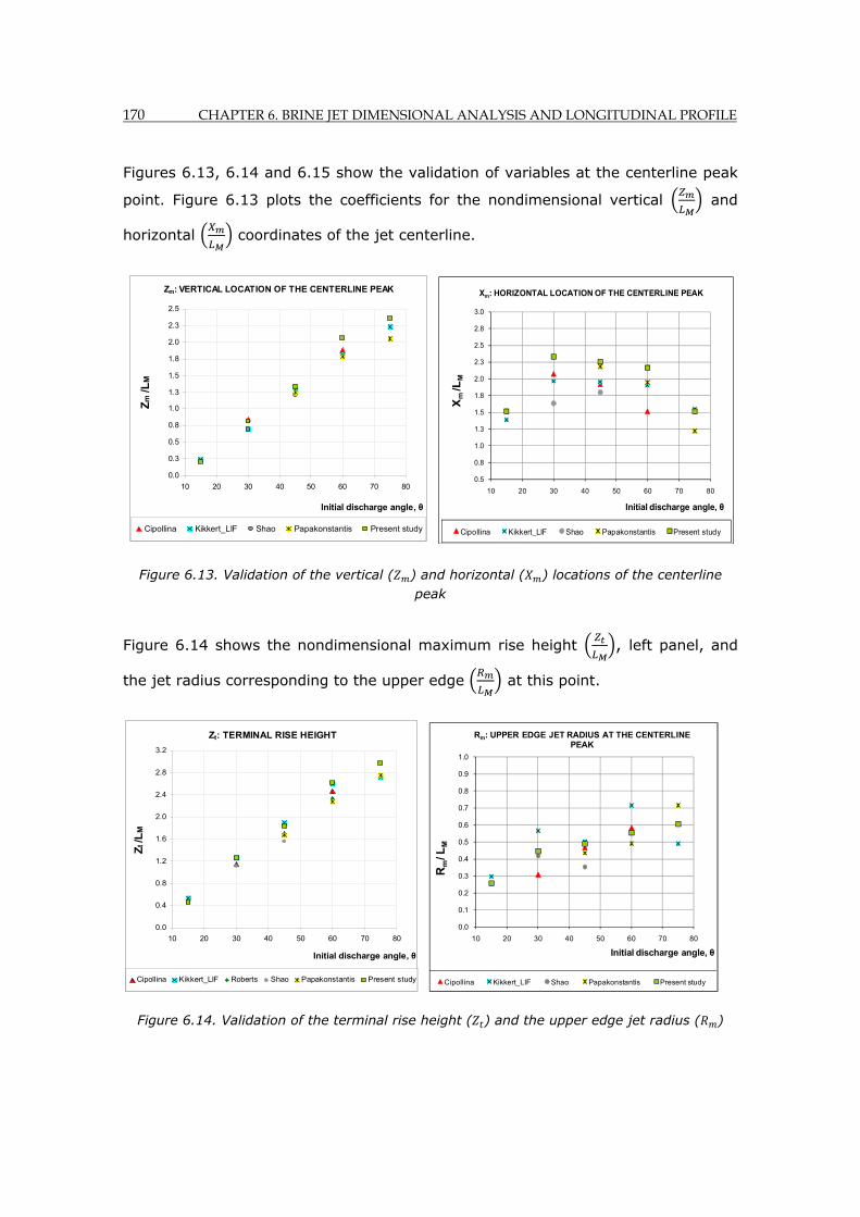
170 CHAPTER 6. BRINE JET DIMENSIONAL ANALYSIS AND LONGITUDINAL PROFILE
Figures 6.13, 6.14 and 6.15 show the validation of variables at the centerline peak
point. Figure 6.13 plots the coefficients for the nondimensional vertical and
horizontal coordinates of the jet centerline.
Figure 6.13. Validation of the vertical ( ) and horizontal ( ) locations of the centerline peak
Figure 6.14 shows the nondimensional maximum rise height , left panel, and
the jet radius corresponding to the upper edge at this point.
Figure 6.14. Validation of the terminal rise height ( ) and the upper edge jet radius ( )
Zm: VERTICAL LOCATION OF THE CENTERLINE PEAK
0.0
0.3
0.5
0.8
1.0
1.3
1.5
1.8
2.0
2.3
2.5
10 20 30 40 50 60 70 80
Initial discharge angle, θ
Zm
/LM
Cipollina Kikkert_LIF Shao Papakonstantis Present study
0.5
0.8
1.0
1.3
1.5
1.8
2.0
2.3
2.5
2.8
3.0
10 20 30 40 50 60 70 80
Xm
/LM
Initial discharge angle, θ
Xm: HORIZONTAL LOCATION OF THE CENTERLINE PEAK
Cipollina Kikkert_LIF Shao Papakonstantis Present study
Zt: TERMINAL RISE HEIGHT
0.0
0.4
0.8
1.2
1.6
2.0
2.4
2.8
3.2
10 20 30 40 50 60 70 80
Initial discharge angle, θ
Zt /L
M
Cipollina Kikkert_LIF Roberts Shao Papakonstantis Present study
0.0
0.1
0.2
0.3
0.4
0.5
0.6
0.7
0.8
0.9
1.0
10 20 30 40 50 60 70 80
Rm
/ LM
Initial discharge angle, θ
Rm: UPPER EDGE JET RADIUS AT THE CENTERLINE PEAK
Cipollina Kikkert_LIF Shao Papakonstantis Present study
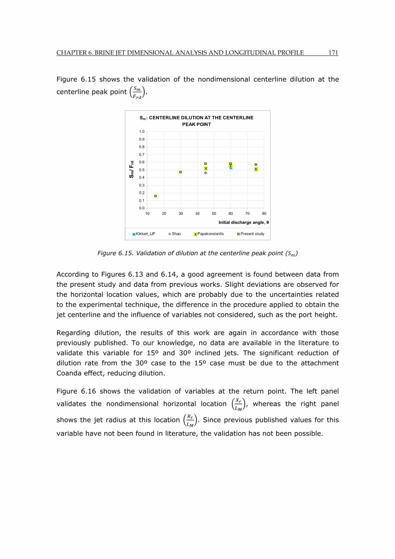
CHAPTER 6. BRINE JET DIMENSIONAL ANALYSIS AND LONGITUDINAL PROFILE 171
Figure 6.15 shows the validation of the nondimensional centerline dilution at the
centerline peak point .
Figure 6.15. Validation of dilution at the centerline peak point ( )
According to Figures 6.13 and 6.14, a good agreement is found between data from
the present study and data from previous works. Slight deviations are observed for
the horizontal location values, which are probably due to the uncertainties related
to the experimental technique, the difference in the procedure applied to obtain the
jet centerline and the influence of variables not considered, such as the port height.
Regarding dilution, the results of this work are again in accordance with those
previously published. To our knowledge, no data are available in the literature to
validate this variable for 15º and 30º inclined jets. The significant reduction of
dilution rate from the 30º case to the 15º case must be due to the attachment
Coanda effect, reducing dilution.
Figure 6.16 shows the validation of variables at the return point. The left panel
validates the nondimensional horizontal location , whereas the right panel
shows the jet radius at this location . Since previous published values for this
variable have not been found in literature, the validation has not been possible.
Sm: CENTERLINE DILUTION AT THE CENTERLINE
PEAK POINT
0.0
0.1
0.2
0.3
0.4
0.5
0.6
0.7
0.8
0.9
1.0
10 20 30 40 50 60 70 80
Initial discharge angle, θ
Sm
/ Frd
Kikkert_LIF Shao Papakonstantis Present study
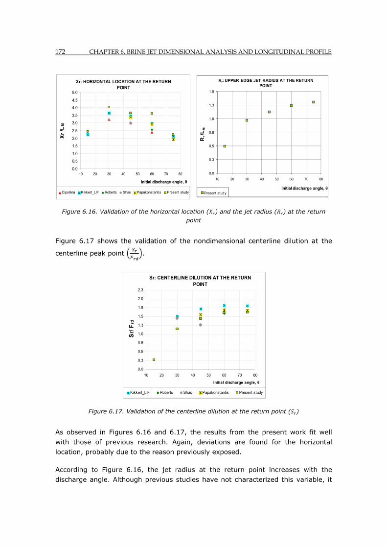
172 CHAPTER 6. BRINE JET DIMENSIONAL ANALYSIS AND LONGITUDINAL PROFILE
Figure 6.16. Validation of the horizontal location ( ) and the jet radius ( ) at the return point
Figure 6.17 shows the validation of the nondimensional centerline dilution at the
centerline peak point .
Figure 6.17. Validation of the centerline dilution at the return point ( )
As observed in Figures 6.16 and 6.17, the results from the present work fit well
with those of previous research. Again, deviations are found for the horizontal
location, probably due to the reason previously exposed.
According to Figure 6.16, the jet radius at the return point increases with the
discharge angle. Although previous studies have not characterized this variable, it
Xr: HORIZONTAL LOCATION AT THE RETURN POINT
0.0
0.5
1.0
1.5
2.0
2.5
3.0
3.5
4.0
4.5
5.0
10 20 30 40 50 60 70 80
Initial discharge angle, θ
Xr
/LM
Cipollina Kikkert_LIF Roberts Shao Papakonstantis Present study
Sr: CENTERLINE DILUTION AT THE RETURN POINT
0.0
0.3
0.5
0.8
1.0
1.3
1.5
1.8
2.0
2.3
10 20 30 40 50 60 70 80
Initial discharge angle, θ
Sr/
Frd
Kikkert_LIF Roberts Shao Papakonstantis Present study
0.0
0.3
0.5
0.8
1.0
1.3
1.5
10 20 30 40 50 60 70 80
Rr /L
M
Initial discharge angle, θ
Rr: UPPER EDGE JET RADIUS AT THE RETURN POINT
Present study
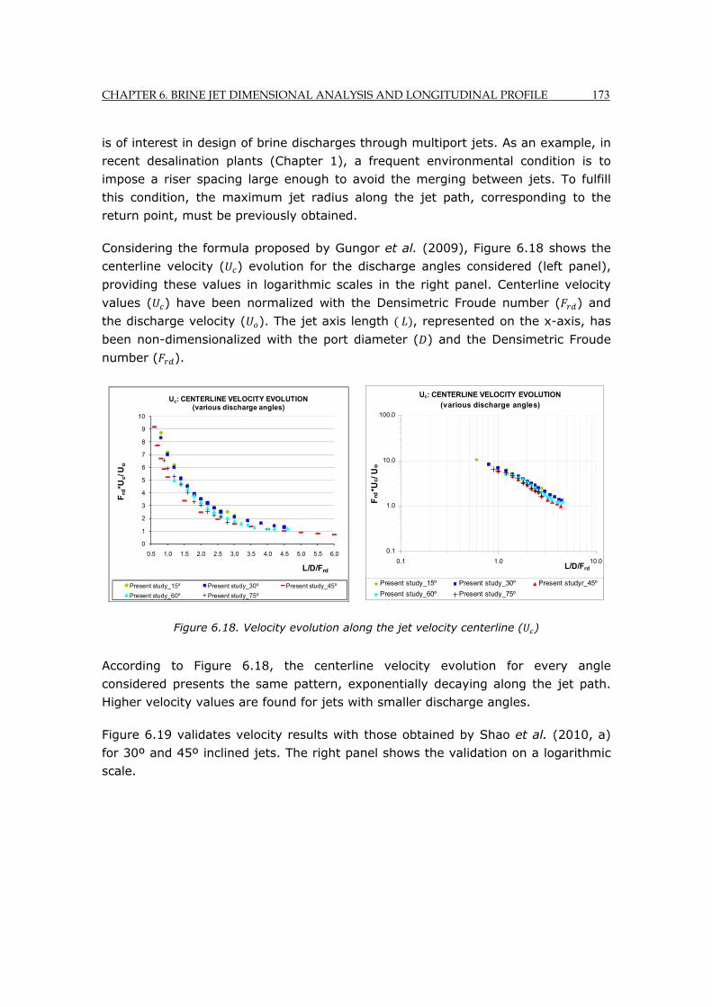
CHAPTER 6. BRINE JET DIMENSIONAL ANALYSIS AND LONGITUDINAL PROFILE 173
is of interest in design of brine discharges through multiport jets. As an example, in
recent desalination plants (Chapter 1), a frequent environmental condition is to
impose a riser spacing large enough to avoid the merging between jets. To fulfill
this condition, the maximum jet radius along the jet path, corresponding to the
return point, must be previously obtained.
Considering the formula proposed by Gungor et al. (2009), Figure 6.18 shows the
centerline velocity ( ) evolution for the discharge angles considered (left panel),
providing these values in logarithmic scales in the right panel. Centerline velocity
values ( ) have been normalized with the Densimetric Froude number ( ) and
the discharge velocity ( ). The jet axis length , represented on the x-axis, has
been non-dimensionalized with the port diameter ( ) and the Densimetric Froude
number ( ).
Figure 6.18. Velocity evolution along the jet velocity centerline ( )
According to Figure 6.18, the centerline velocity evolution for every angle
considered presents the same pattern, exponentially decaying along the jet path.
Higher velocity values are found for jets with smaller discharge angles.
Figure 6.19 validates velocity results with those obtained by Shao et al. (2010, a)
for 30º and 45º inclined jets. The right panel shows the validation on a logarithmic
scale.
0
1
2
3
4
5
6
7
8
9
10
0.5 1.0 1.5 2.0 2.5 3.0 3.5 4.0 4.5 5.0 5.5 6.0
Frd
*Uc/ U
o
L/D/Frd
Uc: CENTERLINE VELOCITY EVOLUTION (various discharge angles)
Present study_15º Present study_30º Present study_45º
Present study_60º Present study_75º
Uc: CENTERLINE VELOCITY EVOLUTION (various discharge angles)
0.1
1.0
10.0
100.0
0.1 1.0 10.0L/D/Frd
Frd
*Uc/
Uo
Present study_15º Present study_30º Present studyr_45º
Present study_60º Present study_75º
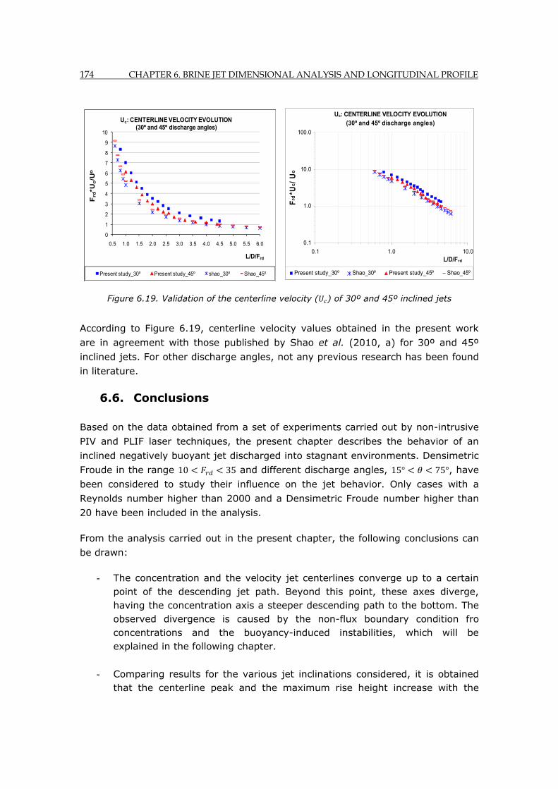
174 CHAPTER 6. BRINE JET DIMENSIONAL ANALYSIS AND LONGITUDINAL PROFILE
Figure 6.19. Validation of the centerline velocity ( ) of 30º and 45º inclined jets
According to Figure 6.19, centerline velocity values obtained in the present work
are in agreement with those published by Shao et al. (2010, a) for 30º and 45º
inclined jets. For other discharge angles, not any previous research has been found
in literature.
6.6. Conclusions
Based on the data obtained from a set of experiments carried out by non-intrusive
PIV and PLIF laser techniques, the present chapter describes the behavior of an
inclined negatively buoyant jet discharged into stagnant environments. Densimetric
Froude in the range 10 35 and different discharge angles, 15° 75°, have
been considered to study their influence on the jet behavior. Only cases with a
Reynolds number higher than 2000 and a Densimetric Froude number higher than
20 have been included in the analysis.
From the analysis carried out in the present chapter, the following conclusions can
be drawn:
- The concentration and the velocity jet centerlines converge up to a certain point of the descending jet path. Beyond this point, these axes diverge, having the concentration axis a steeper descending path to the bottom. The observed divergence is caused by the non-flux boundary condition fro concentrations and the buoyancy-induced instabilities, which will be explained in the following chapter.
- Comparing results for the various jet inclinations considered, it is obtained that the centerline peak and the maximum rise height increase with the
0
1
2
3
4
5
6
7
8
9
10
0.5 1.0 1.5 2.0 2.5 3.0 3.5 4.0 4.5 5.0 5.5 6.0
Frd
*Uc/U
o
L/D/Frd
Uc: CENTERLINE VELOCITY EVOLUTION (30º and 45º discharge angles)
Present study_30º Present study_45º shao_30º Shao_45º
Uc: CENTERLINE VELOCITY EVOLUTION (30º and 45º discharge angles)
0.1
1.0
10.0
100.0
0.1 1.0 10.0L/D/Frd
Frd
*Uc /
Uo
Present study_30º Shao_30º Present study_45º Shao_45º
CHAPTER 6. BRINE JET DIMENSIONAL ANALYSIS AND LONGITUDINAL PROFILE 175
initial discharge angle. However, the horizontal location of the centerline peak and the return point diminishes with this angle. The 15º inclined jet is an exception to this statement since the Coanda effect causes the attachment of the jet to the bottom, reducing the jet length path and dilution radically.
- For the testing angles, centerline dilution increases with the discharge angle up to a maximum obtained for 60º discharge angle. From 60º to 75º, no any additional dilution is achieved. Dilution for a 15º inclined jet is observed to be extremely low, as a consequence of the Coanda effect.
- The dilution rate achieved along the descending path has been found to be significantly higher than that achieved along the upward trajectory in all cases. Furthermore, dilution at the return point is observed to be appreciably higher than dilution at the impact point. This statement, which has not been previously reported, requires to be considered in discharge design in order to consider the most unfavourable conditions.
- Regarding the hydrodynamic variables, the horizontal component of the centerline velocity decreases from the nozzle up to the impact point in all cases. For the same horizontal location (x), the horizontal velocity is always higher for jets with lower inclinations. For highly inclined jets (60º and 75º cases), the horizontal velocity is close to zero in the downward jet motion since the descending jet trajectory is almost vertical.
- Comparing both components of centerline velocity, the vertical velocity is observed to decrease more rapidly than the horizontal counterpart.
- Considering the variables along the velocity and concentration centerline together, it seems that the centerline dilution depends on the vertical component of velocity and on the jet axis length. According to the analysis carried out, the dilution rate increases with both variables, which present maximum values for 60º and 75º inclined jets. Therefore, the dilution achieved is maximum for these cases.
- The dimensional analysis formulas proposed in the present work allow a preliminary prediction of the jet behavior for real cases, which can be used in brine discharge designs. Crucial values for discharge designs, not previously reported, has been provided in the present study, such as the jet width or differences in centerline dilution achieved a the return and at the impact point.

176 CHAPTER 6. BRINE JET DIMENSIONAL ANALYSIS AND LONGITUDINAL PROFILE
- The validation carried out with available data found in the literature shows a good agreement between the results of the present research and those found in previous works.
For the first time in literature, simultaneous PIV and PLIF techniques have been used to describe the behavior of negatively buoyant jets, such as those of brine. An extensive range of design parameters has been considered to characterize the velocity and concentration centerline variables.
CHAPTER 7. BRINE JET FLOW FIELDS AND TRANSVERSE PROFILES 177
Chapter 7. BRINE JET FLOW FIEDS AND TRANSVERSE PROFILES BASED ON THE EXPERIMENTAL DATA ANALYSIS
Chapter 7 BRINE JET FLOW FIELDS AND TRANSVERSE PROFILES BASED ON THE ANALYSIS OF EXPERIMENTAL DATA
Summary
The present chapter continues with the analysis of the PIV and PLIF experimental
data obtained in the present work to characterize the behavior of a submerged and
inclined brine jet discharge.
The previous chapter has focused on the analysis of variables along the jet
centerlines and has provided experimental coefficients for dimensional analysis
formulas at specific points of the jet path. The present chapter aims to deepen into
the hydrodynamic and mixing processes that control the jet behavior and the
differences from a typical neutral jet.
The average and turbulent flow-fields of the jet path are analyzed first, including
velocity components, vorticity, dilution rate and snapshot images of the flow, in
order to go deeper into the processes involved in the brine jet behavior. Next,
cross-sections are obtained, studying their evolution along the jet path.
Nondimensional profiles, self-similarity properties and profile shapes are studied to
assess the reliability of the hypothesis generally assumed by numerical integral
models. The results reveal significant divergence relative to the classical behavior of
a round jet without curvature.
178 CHAPTER 7. BRINE JET FLOW FIELDS AND TRANSVERSE PROFILES
7.1. Introduction
This chapter is the second part of the analysis of the PLIF and PIV experimental
data obtained to characterize the jet path in the present work. While Chapter 7
focused on the characterization of variables along the jet axes and the calibration of
dimensional analysis formulas, this chapter goes in depth into the flow
hydrodynamic and mixing processes.
There are very few preliminary works characterizing negatively buoyant jets from
the point of view of the present chapter, which deepens in the flow processes to
understand the special features of this type of jets. In Kikkert et al. (2007), 30º,
45º and 60º inclined dense jets were studied using PLIF and the averaged
concentration cross-sections were characterized. A more extensive experimental
research using PIV and PLIF was carried out in Shao et al. (2010, a), analyzing the
concentration and velocity transverse profiles of 30º and 45º dense inclined jets.
However, the profiles characterized were limited to locations close to the nozzle,
where the behavior is similar to that of neutral jets. An in-depth analysis of flow
processes was presented in Shao et al. (2009), analyzing the turbulent variables
and momentum transport, but the study was limited to circular offset horizontal
dense jets. An exhaustive study of the processes involved in the behavior of
negatively buoyant jets was carried out by Wang et al. (2002). The flow integral
governing equations were improved by including additional second order terms for
a better fit to experimental data. However, the study focused on vertical jets only.
According to this, there is still a need for characterizing the processes governing
inclined negatively buoyant jets, such as those of brine, covering the range of
discharge angles generally used in actual desalination plants. Furthermore, the
special features of this type of dense inclined jets require to be characterized in
order to assess the simplifying hypothesis generally assumed by numerical
approaches. This study will contribute to our understanding of why commercial
models do not correctly simulate brine discharges, providing useful information to
re-calibrate numerical models.
The analysis presented here bases on the case study of the previous chapter,
covering dense jets with discharge angles in the range: 15° 75° and
Densimetric Froude number in the range: 10 35. The study begins with the
analysis of the flow-fields related to the hydrodynamic and mixing processes within
the flow. The analysis considers the velocity modulus and components, the
vorticity, the dilution, snapshots images, etc., comparing the jet behavior for
different discharge angles. Concentration and velocity transverse profiles along the
jet path are next characterized, including the averaged and turbulent components
of variables. Non-dimensionalized profiles, self-similarity and Gaussian shape
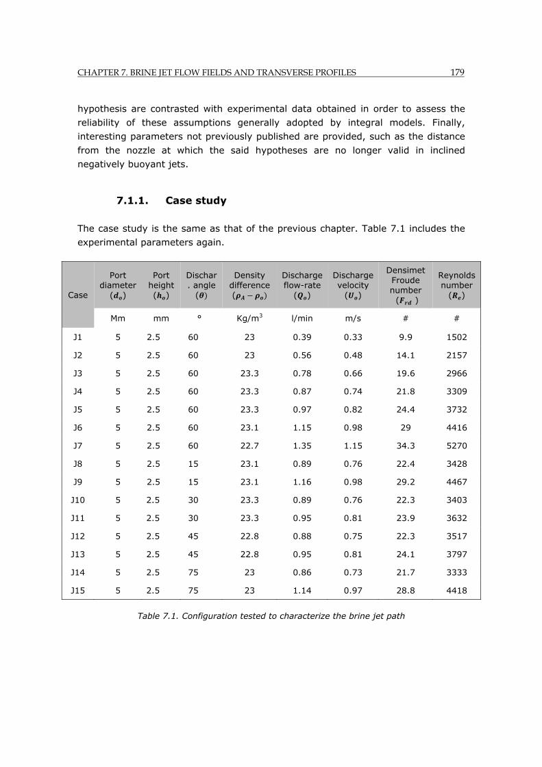
CHAPTER 7. BRINE JET FLOW FIELDS AND TRANSVERSE PROFILES 179
hypothesis are contrasted with experimental data obtained in order to assess the
reliability of these assumptions generally adopted by integral models. Finally,
interesting parameters not previously published are provided, such as the distance
from the nozzle at which the said hypotheses are no longer valid in inclined
negatively buoyant jets.
7.1.1. Case study
The case study is the same as that of the previous chapter. Table 7.1 includes the
experimental parameters again.
Case
Port diameter
( )
Port height ( )
Dischar. angle
(
Density difference (
Discharge flow-rate
( )
Discharge velocity
( )
Densimet Froude number ( )
Reynolds number
( )
Mm mm ° Kg/m3 l/min m/s # #
J1 5 2.5 60 23 0.39 0.33 9.9 1502
J2 5 2.5 60 23 0.56 0.48 14.1 2157
J3 5 2.5 60 23.3 0.78 0.66 19.6 2966
J4 5 2.5 60 23.3 0.87 0.74 21.8 3309
J5 5 2.5 60 23.3 0.97 0.82 24.4 3732
J6 5 2.5 60 23.1 1.15 0.98 29 4416
J7 5 2.5 60 22.7 1.35 1.15 34.3 5270
J8 5 2.5 15 23.1 0.89 0.76 22.4 3428
J9 5 2.5 15 23.1 1.16 0.98 29.2 4467
J10 5 2.5 30 23.3 0.89 0.76 22.3 3403
J11 5 2.5 30 23.3 0.95 0.81 23.9 3632
J12 5 2.5 45 22.8 0.88 0.75 22.3 3517
J13 5 2.5 45 22.8 0.95 0.81 24.1 3797
J14 5 2.5 75 23 0.86 0.73 21.7 3333
J15 5 2.5 75 23 1.14 0.97 28.8 4418
Table 7.1. Configuration tested to characterize the brine jet path
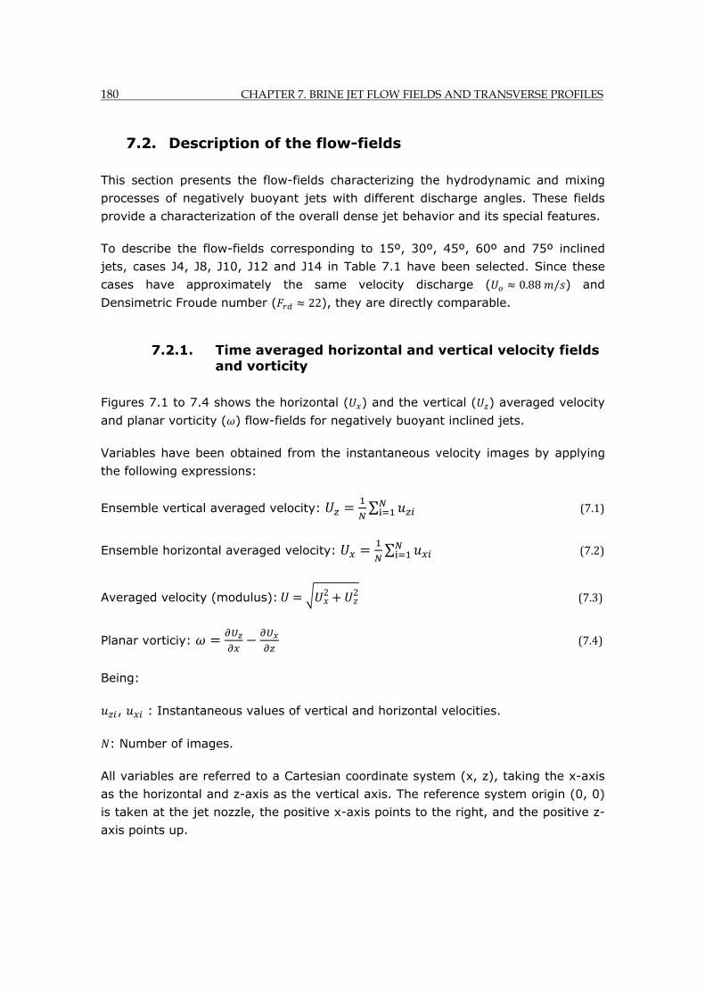
180 CHAPTER 7. BRINE JET FLOW FIELDS AND TRANSVERSE PROFILES
7.2. Description of the flow-fields
This section presents the flow-fields characterizing the hydrodynamic and mixing
processes of negatively buoyant jets with different discharge angles. These fields
provide a characterization of the overall dense jet behavior and its special features.
To describe the flow-fields corresponding to 15º, 30º, 45º, 60º and 75º inclined
jets, cases J4, J8, J10, J12 and J14 in Table 7.1 have been selected. Since these
cases have approximately the same velocity discharge ( 0.88 / ) and
Densimetric Froude number ( 22), they are directly comparable.
7.2.1. Time averaged horizontal and vertical velocity fields and vorticity
Figures 7.1 to 7.4 shows the horizontal ( ) and the vertical ( ) averaged velocity
and planar vorticity ( ) flow-fields for negatively buoyant inclined jets.
Variables have been obtained from the instantaneous velocity images by applying
the following expressions:
Ensemble vertical averaged velocity: ∑ (7.1)
Ensemble horizontal averaged velocity: ∑ (7.2)
Averaged velocity (modulus): 2 2 (7.3)
Planar vorticiy: (7.4)
Being:
, : Instantaneous values of vertical and horizontal velocities.
: Number of images.
All variables are referred to a Cartesian coordinate system (x, z), taking the x-axis
as the horizontal and z-axis as the vertical axis. The reference system origin (0, 0)
is taken at the jet nozzle, the positive x-axis points to the right, and the positive z-
axis points up.
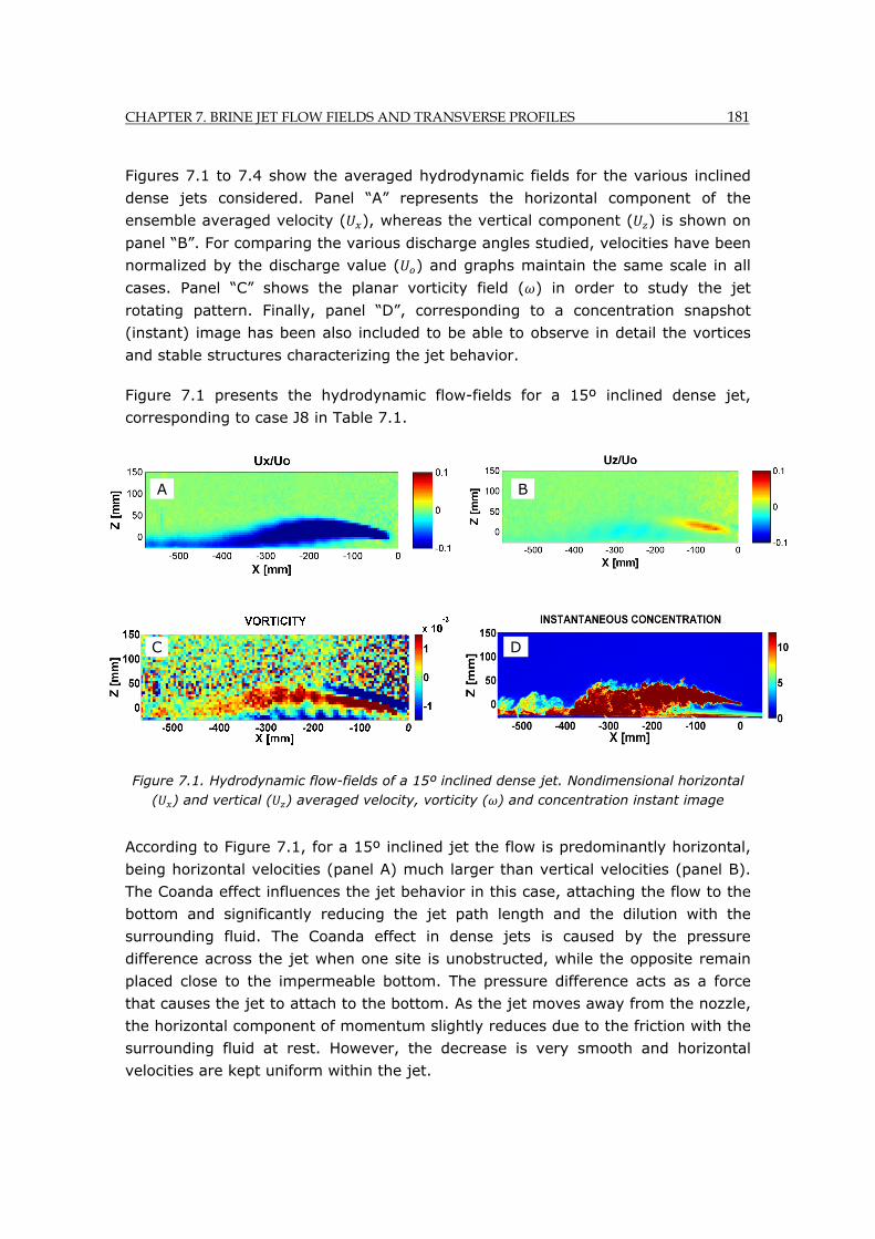
CHAPTER 7. BRINE JET FLOW FIELDS AND TRANSVERSE PROFILES 181
Figures 7.1 to 7.4 show the averaged hydrodynamic fields for the various inclined
dense jets considered. Panel “A” represents the horizontal component of the
ensemble averaged velocity ( ), whereas the vertical component ( ) is shown on
panel “B”. For comparing the various discharge angles studied, velocities have been
normalized by the discharge value ( ) and graphs maintain the same scale in all
cases. Panel “C” shows the planar vorticity field ( ) in order to study the jet
rotating pattern. Finally, panel “D”, corresponding to a concentration snapshot
(instant) image has been also included to be able to observe in detail the vortices
and stable structures characterizing the jet behavior.
Figure 7.1 presents the hydrodynamic flow-fields for a 15º inclined dense jet,
corresponding to case J8 in Table 7.1.
Figure 7.1. Hydrodynamic flow-fields of a 15º inclined dense jet. Nondimensional horizontal ( ) and vertical ( ) averaged velocity, vorticity ( ) and concentration instant image
According to Figure 7.1, for a 15º inclined jet the flow is predominantly horizontal,
being horizontal velocities (panel A) much larger than vertical velocities (panel B).
The Coanda effect influences the jet behavior in this case, attaching the flow to the
bottom and significantly reducing the jet path length and the dilution with the
surrounding fluid. The Coanda effect in dense jets is caused by the pressure
difference across the jet when one site is unobstructed, while the opposite remain
placed close to the impermeable bottom. The pressure difference acts as a force
that causes the jet to attach to the bottom. As the jet moves away from the nozzle,
the horizontal component of momentum slightly reduces due to the friction with the
surrounding fluid at rest. However, the decrease is very smooth and horizontal
velocities are kept uniform within the jet.
B A
C D
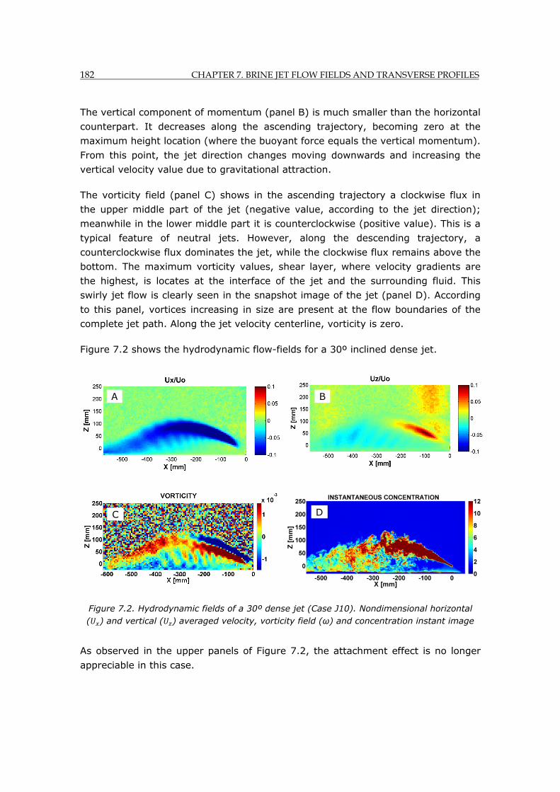
182 CHAPTER 7. BRINE JET FLOW FIELDS AND TRANSVERSE PROFILES
The vertical component of momentum (panel B) is much smaller than the horizontal
counterpart. It decreases along the ascending trajectory, becoming zero at the
maximum height location (where the buoyant force equals the vertical momentum).
From this point, the jet direction changes moving downwards and increasing the
vertical velocity value due to gravitational attraction.
The vorticity field (panel C) shows in the ascending trajectory a clockwise flux in
the upper middle part of the jet (negative value, according to the jet direction);
meanwhile in the lower middle part it is counterclockwise (positive value). This is a
typical feature of neutral jets. However, along the descending trajectory, a
counterclockwise flux dominates the jet, while the clockwise flux remains above the
bottom. The maximum vorticity values, shear layer, where velocity gradients are
the highest, is locates at the interface of the jet and the surrounding fluid. This
swirly jet flow is clearly seen in the snapshot image of the jet (panel D). According
to this panel, vortices increasing in size are present at the flow boundaries of the
complete jet path. Along the jet velocity centerline, vorticity is zero.
Figure 7.2 shows the hydrodynamic flow-fields for a 30º inclined dense jet.
Figure 7.2. Hydrodynamic fields of a 30º dense jet (Case J10). Nondimensional horizontal ( ) and vertical ( ) averaged velocity, vorticity field (ω) and concentration instant image
As observed in the upper panels of Figure 7.2, the attachment effect is no longer
appreciable in this case.
A B
C D
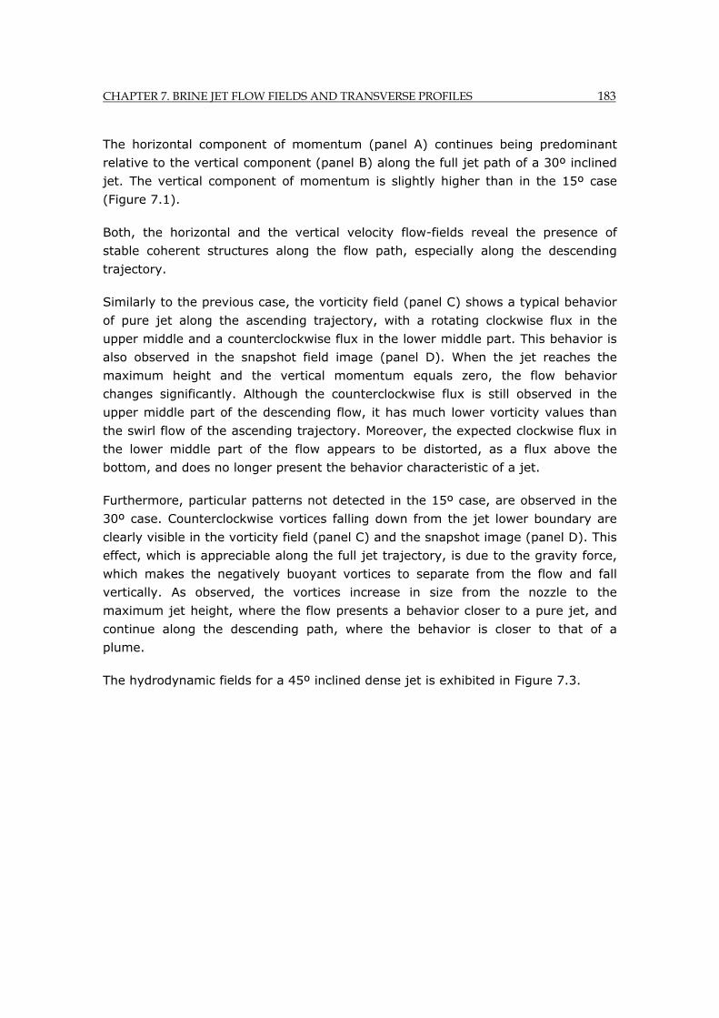
CHAPTER 7. BRINE JET FLOW FIELDS AND TRANSVERSE PROFILES 183
The horizontal component of momentum (panel A) continues being predominant
relative to the vertical component (panel B) along the full jet path of a 30º inclined
jet. The vertical component of momentum is slightly higher than in the 15º case
(Figure 7.1).
Both, the horizontal and the vertical velocity flow-fields reveal the presence of
stable coherent structures along the flow path, especially along the descending
trajectory.
Similarly to the previous case, the vorticity field (panel C) shows a typical behavior
of pure jet along the ascending trajectory, with a rotating clockwise flux in the
upper middle and a counterclockwise flux in the lower middle part. This behavior is
also observed in the snapshot field image (panel D). When the jet reaches the
maximum height and the vertical momentum equals zero, the flow behavior
changes significantly. Although the counterclockwise flux is still observed in the
upper middle part of the descending flow, it has much lower vorticity values than
the swirl flow of the ascending trajectory. Moreover, the expected clockwise flux in
the lower middle part of the flow appears to be distorted, as a flux above the
bottom, and does no longer present the behavior characteristic of a jet.
Furthermore, particular patterns not detected in the 15º case, are observed in the
30º case. Counterclockwise vortices falling down from the jet lower boundary are
clearly visible in the vorticity field (panel C) and the snapshot image (panel D). This
effect, which is appreciable along the full jet trajectory, is due to the gravity force,
which makes the negatively buoyant vortices to separate from the flow and fall
vertically. As observed, the vortices increase in size from the nozzle to the
maximum jet height, where the flow presents a behavior closer to a pure jet, and
continue along the descending path, where the behavior is closer to that of a
plume.
The hydrodynamic fields for a 45º inclined dense jet is exhibited in Figure 7.3.
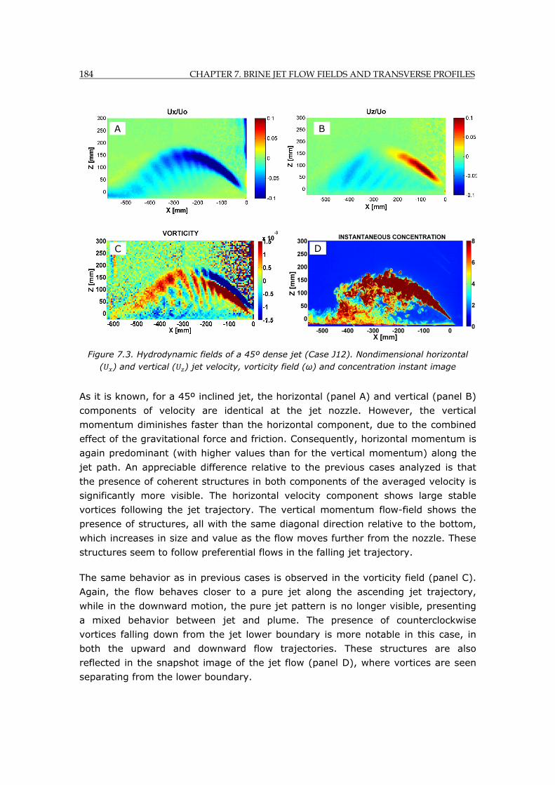
184 CHAPTER 7. BRINE JET FLOW FIELDS AND TRANSVERSE PROFILES
Figure 7.3. Hydrodynamic fields of a 45º dense jet (Case J12). Nondimensional horizontal ( ) and vertical ( ) jet velocity, vorticity field (ω) and concentration instant image
As it is known, for a 45º inclined jet, the horizontal (panel A) and vertical (panel B)
components of velocity are identical at the jet nozzle. However, the vertical
momentum diminishes faster than the horizontal component, due to the combined
effect of the gravitational force and friction. Consequently, horizontal momentum is
again predominant (with higher values than for the vertical momentum) along the
jet path. An appreciable difference relative to the previous cases analyzed is that
the presence of coherent structures in both components of the averaged velocity is
significantly more visible. The horizontal velocity component shows large stable
vortices following the jet trajectory. The vertical momentum flow-field shows the
presence of structures, all with the same diagonal direction relative to the bottom,
which increases in size and value as the flow moves further from the nozzle. These
structures seem to follow preferential flows in the falling jet trajectory.
The same behavior as in previous cases is observed in the vorticity field (panel C).
Again, the flow behaves closer to a pure jet along the ascending jet trajectory,
while in the downward motion, the pure jet pattern is no longer visible, presenting
a mixed behavior between jet and plume. The presence of counterclockwise
vortices falling down from the jet lower boundary is more notable in this case, in
both the upward and downward flow trajectories. These structures are also
reflected in the snapshot image of the jet flow (panel D), where vortices are seen
separating from the lower boundary.
A B
C D
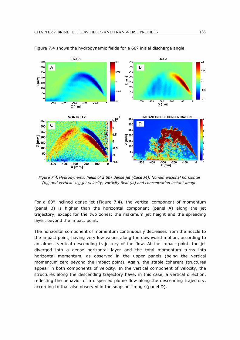
CHAPTER 7. BRINE JET FLOW FIELDS AND TRANSVERSE PROFILES 185
Figure 7.4 shows the hydrodynamic fields for a 60º initial discharge angle.
For a 60º inclined dense jet (Figure 7.4), the vertical component of momentum
(panel B) is higher than the horizontal component (panel A) along the jet
trajectory, except for the two zones: the maximum jet height and the spreading
layer, beyond the impact point.
The horizontal component of momentum continuously decreases from the nozzle to
the impact point, having very low values along the downward motion, according to
an almost vertical descending trajectory of the flow. At the impact point, the jet
diverged into a dense horizontal layer and the total momentum turns into
horizontal momentum, as observed in the upper panels (being the vertical
momentum zero beyond the impact point). Again, the stable coherent structures
appear in both components of velocity. In the vertical component of velocity, the
structures along the descending trajectory have, in this case, a vertical direction,
reflecting the behavior of a dispersed plume flow along the descending trajectory,
according to that also observed in the snapshot image (panel D).
A
C D
B
Figure 7 4. Hydrodynamic fields of a 60º dense jet (Case J4). Nondimensional horizontal ( ) and vertical ( ) jet velocity, vorticity field (ω) and concentration instant image
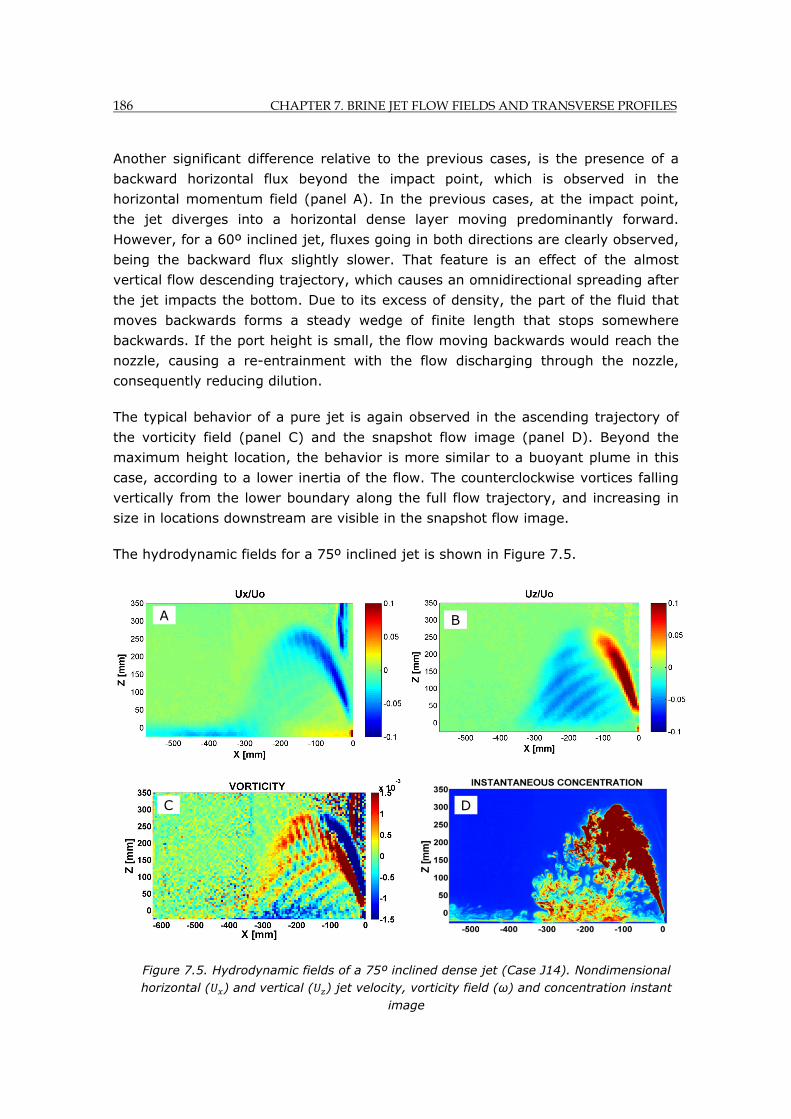
186 CHAPTER 7. BRINE JET FLOW FIELDS AND TRANSVERSE PROFILES
Another significant difference relative to the previous cases, is the presence of a
backward horizontal flux beyond the impact point, which is observed in the
horizontal momentum field (panel A). In the previous cases, at the impact point,
the jet diverges into a horizontal dense layer moving predominantly forward.
However, for a 60º inclined jet, fluxes going in both directions are clearly observed,
being the backward flux slightly slower. That feature is an effect of the almost
vertical flow descending trajectory, which causes an omnidirectional spreading after
the jet impacts the bottom. Due to its excess of density, the part of the fluid that
moves backwards forms a steady wedge of finite length that stops somewhere
backwards. If the port height is small, the flow moving backwards would reach the
nozzle, causing a re-entrainment with the flow discharging through the nozzle,
consequently reducing dilution.
The typical behavior of a pure jet is again observed in the ascending trajectory of
the vorticity field (panel C) and the snapshot flow image (panel D). Beyond the
maximum height location, the behavior is more similar to a buoyant plume in this
case, according to a lower inertia of the flow. The counterclockwise vortices falling
vertically from the lower boundary along the full flow trajectory, and increasing in
size in locations downstream are visible in the snapshot flow image.
The hydrodynamic fields for a 75º inclined jet is shown in Figure 7.5.
A
B
C
A
Figure 7.5. Hydrodynamic fields of a 75º inclined dense jet (Case J14). Nondimensional horizontal ( ) and vertical ( ) jet velocity, vorticity field (ω) and concentration instant
image
D
CHAPTER 7. BRINE JET FLOW FIELDS AND TRANSVERSE PROFILES 187
As observed in Figure 7.5, the vertical momentum (panel B) is clearly higher than
the horizontal momentum (panel A) along the full jet path up to the impact point of
a 75º inclined jet.
The vertical component of momentum (panel B) has a similar behavior to that of a
60º case. Large coherent structures are observed along the descending path,
characterizing a dispersed flow typical of plumes, with preferential flows. In this
case, as the horizontal momentum is lower, the flow inertia is lower, being
approximately zero at the descending path, implying an almost pure plume
behavior in this zone.
As in previous cases, the horizontal component of momentum gradually decreases
from the nozzle to the impact point. At this point, the jet diverges into a horizontal
dense layer, appearing forward and backward fluxes of the same value moving
above the bottom, in a round radial shape from the stagnation point. This
omnidirectional spreading is related to the almost vertical jet trajectory at the
impact point in this case. The coherent structures are more visible than in the
previous cases in the vertical velocity field (panel B), being smoother and less
evident in the horizontal velocity field (panel A).
Regarding the planar vorticity (panel C), again the ascending path presents the
pattern typical of a pure jet. The counterclockwise hyperdense vortices separating
from the flow and falling down from the lower jet boundary are more visible in this
case, beginning practically at the jet nozzle. Along the descending trajectory, the
flow does no longer behave as a jet, being the inertia almost zero, while the
buoyancy completely dominates the flow, which is characterized by a cascade of
swirl flow falling with both vorticity directions, as observed in the vorticity field and
the snapshot image (panel D).
According to the analysis carried out, the following conclusions can be drawn:
- Horizontal momentum (panels A) smoothly decreases from the nozzle to the impact point in all cases. At the impact point, the total momentum turns into horizontal momentum and the jet diverges into a horizontal dense layer. For jets with low inclinations (15º and 30º), this layer moves overall forward, in the jet discharge direction. However, for highly inclined jets (60º and 75º), the spreading layer expands in all directions (as a consequence of a vertical impingement jet trajectory) and fluxes moving forwards and backwards from the stagnation point can be observed in the horizontal momentum field. Large stable vortices following the jet path are also observed in this field.
- Vertical momentum (panels B) decreases along the ascending trajectory more rapidly than the horizontal counterpart, due to the combined effect of
188 CHAPTER 7. BRINE JET FLOW FIELDS AND TRANSVERSE PROFILES
the gravity force and friction. Along the downwards trajectory, the vertical momentum is characterized by a dispersed flow with increasing velocity values due to the gravity acceleration. Coherent structures are also relevant, increasing in size along the downstream direction and showing preferential flows along the descending path.
- Vorticity fields (panels C) show common patterns to all cases. The ascending trajectory has a behavior close to a pure jet, with counterclockwise vortices in the upper middle part and a clockwise flux in the lower counterpart. Beyond the maximum centerline peal point, the flow does no longer present the pure jet patterns and behaves as a transition flow between jet and plume. While a flux rotating counterclockwise is observed along the upper boundary of the descending trajectory, the lower boundary appears to be distorted due to the fall of counterclockwise vortices from the lower edge, generating instabilities within this zone. This feature, which is more notable in highly inclined jets, occurs along the full jet path and it is caused by the gravitational force. This force makes the hyperdense vortices to separate from the flow and descends almost vertically.
- The swirl flow shown in the vorticity field is also visible in the snapshot images of the flow (panels D), where the jet and plume behavior along the jet path and the vortices falling from the lower edge can be clearly observed. This last feature is expected to be an additional dilution process, as the vortices separating from the flow increase the entrainment and the potential area of mixing between both fluids. This particular behavior of inclined negatively buoyant jets was also observed by Papakonstantis et al. (2011, a, b), which mentioned that, beyond the maximum jet height zone, parcels of fluid were observed to separate from the main flow and descend almost vertically to the bottom. In Kikkert et al. (2007) and Shao et al. (2010, a), this flow feature along the inner edge was defined as buoyancy-induced instabilities. The present work goes deeper into the description and physical justification of this process, which must have a significant influence on the inclined dense jets behavior and the dilution rates.
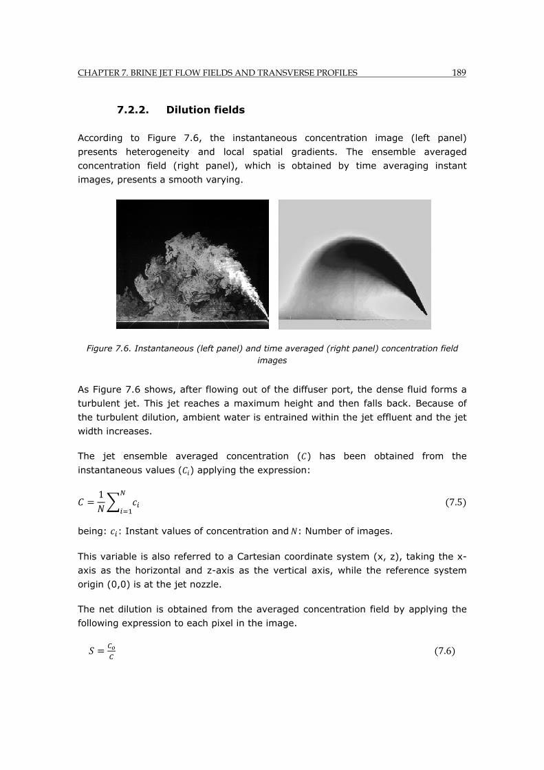
CHAPTER 7. BRINE JET FLOW FIELDS AND TRANSVERSE PROFILES 189
7.2.2. Dilution fields
According to Figure 7.6, the instantaneous concentration image (left panel)
presents heterogeneity and local spatial gradients. The ensemble averaged
concentration field (right panel), which is obtained by time averaging instant
images, presents a smooth varying.
Figure 7.6. Instantaneous (left panel) and time averaged (right panel) concentration field images
As Figure 7.6 shows, after flowing out of the diffuser port, the dense fluid forms a
turbulent jet. This jet reaches a maximum height and then falls back. Because of
the turbulent dilution, ambient water is entrained within the jet effluent and the jet
width increases.
The jet ensemble averaged concentration ( ) has been obtained from the
instantaneous values ( ) applying the expression:
1 7.5
being: : Instant values of concentration and : Number of images.
This variable is also referred to a Cartesian coordinate system (x, z), taking the x-
axis as the horizontal and z-axis as the vertical axis, while the reference system
origin (0,0) is at the jet nozzle.
The net dilution is obtained from the averaged concentration field by applying the
following expression to each pixel in the image.
7.6
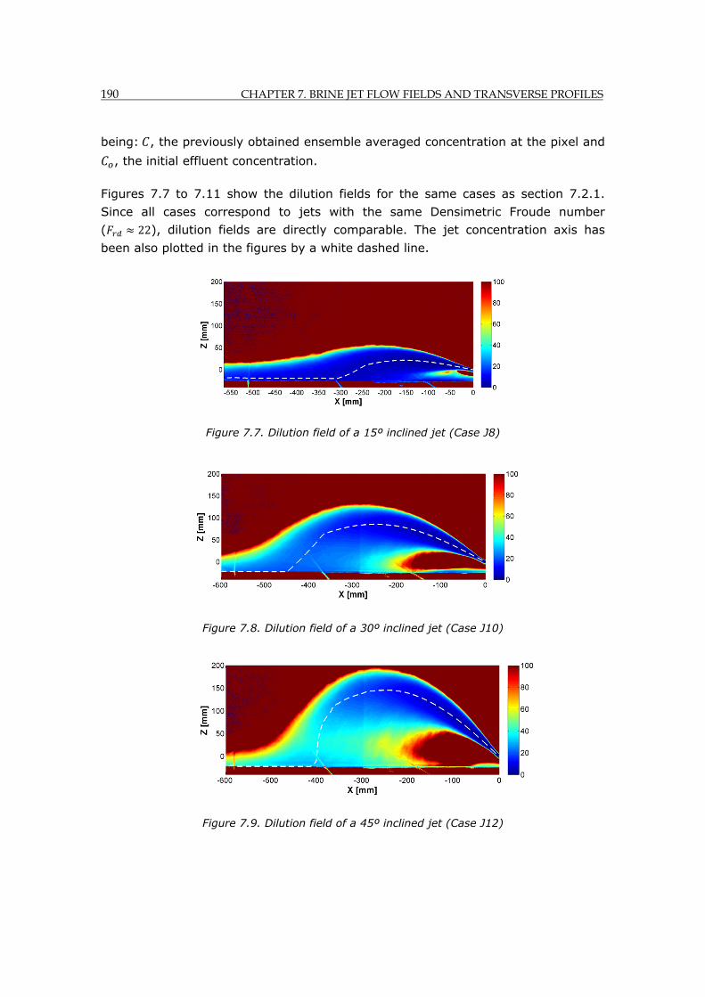
190 CHAPTER 7. BRINE JET FLOW FIELDS AND TRANSVERSE PROFILES
being: , the previously obtained ensemble averaged concentration at the pixel and
, the initial effluent concentration.
Figures 7.7 to 7.11 show the dilution fields for the same cases as section 7.2.1.
Since all cases correspond to jets with the same Densimetric Froude number
( 22), dilution fields are directly comparable. The jet concentration axis has
been also plotted in the figures by a white dashed line.
Figure 7.7. Dilution field of a 15º inclined jet (Case J8)
Figure 7.8. Dilution field of a 30º inclined jet (Case J10)
Figure 7.9. Dilution field of a 45º inclined jet (Case J12)
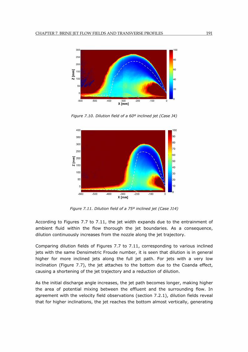
CHAPTER 7. BRINE JET FLOW FIELDS AND TRANSVERSE PROFILES 191
Figure 7.10. Dilution field of a 60º inclined jet (Case J4)
Figure 7.11. Dilution field of a 75º inclined jet (Case J14)
According to Figures 7.7 to 7.11, the jet width expands due to the entrainment of
ambient fluid within the flow thorough the jet boundaries. As a consequence,
dilution continuously increases from the nozzle along the jet trajectory.
Comparing dilution fields of Figures 7.7 to 7.11, corresponding to various inclined
jets with the same Densimetric Froude number, it is seen that dilution is in general
higher for more inclined jets along the full jet path. For jets with a very low
inclination (Figure 7.7), the jet attaches to the bottom due to the Coanda effect,
causing a shortening of the jet trajectory and a reduction of dilution.
As the initial discharge angle increases, the jet path becomes longer, making higher
the area of potential mixing between the effluent and the surrounding flow. In
agreement with the velocity field observations (section 7.2.1), dilution fields reveal
that for higher inclinations, the jet reaches the bottom almost vertically, generating
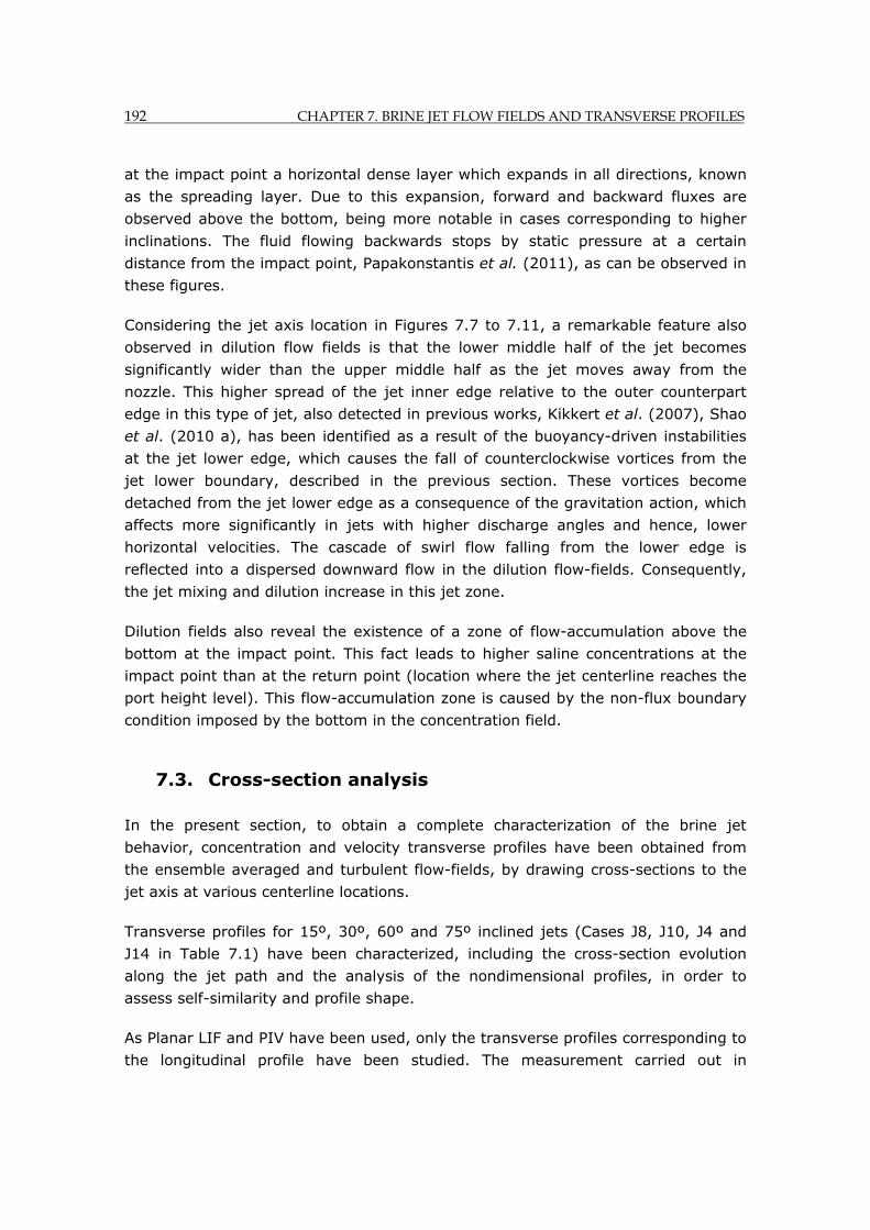
192 CHAPTER 7. BRINE JET FLOW FIELDS AND TRANSVERSE PROFILES
at the impact point a horizontal dense layer which expands in all directions, known
as the spreading layer. Due to this expansion, forward and backward fluxes are
observed above the bottom, being more notable in cases corresponding to higher
inclinations. The fluid flowing backwards stops by static pressure at a certain
distance from the impact point, Papakonstantis et al. (2011), as can be observed in
these figures.
Considering the jet axis location in Figures 7.7 to 7.11, a remarkable feature also
observed in dilution flow fields is that the lower middle half of the jet becomes
significantly wider than the upper middle half as the jet moves away from the
nozzle. This higher spread of the jet inner edge relative to the outer counterpart
edge in this type of jet, also detected in previous works, Kikkert et al. (2007), Shao
et al. (2010 a), has been identified as a result of the buoyancy-driven instabilities
at the jet lower edge, which causes the fall of counterclockwise vortices from the
jet lower boundary, described in the previous section. These vortices become
detached from the jet lower edge as a consequence of the gravitation action, which
affects more significantly in jets with higher discharge angles and hence, lower
horizontal velocities. The cascade of swirl flow falling from the lower edge is
reflected into a dispersed downward flow in the dilution flow-fields. Consequently,
the jet mixing and dilution increase in this jet zone.
Dilution fields also reveal the existence of a zone of flow-accumulation above the
bottom at the impact point. This fact leads to higher saline concentrations at the
impact point than at the return point (location where the jet centerline reaches the
port height level). This flow-accumulation zone is caused by the non-flux boundary
condition imposed by the bottom in the concentration field.
7.3. Cross-section analysis
In the present section, to obtain a complete characterization of the brine jet
behavior, concentration and velocity transverse profiles have been obtained from
the ensemble averaged and turbulent flow-fields, by drawing cross-sections to the
jet axis at various centerline locations.
Transverse profiles for 15º, 30º, 60º and 75º inclined jets (Cases J8, J10, J4 and
J14 in Table 7.1) have been characterized, including the cross-section evolution
along the jet path and the analysis of the nondimensional profiles, in order to
assess self-similarity and profile shape.
As Planar LIF and PIV have been used, only the transverse profiles corresponding to
the longitudinal profile have been studied. The measurement carried out in
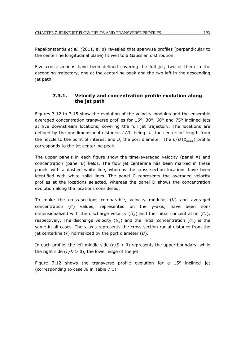
CHAPTER 7. BRINE JET FLOW FIELDS AND TRANSVERSE PROFILES 193
Papakonstantis et al. (2011, a, b) revealed that spanwise profiles (perpendicular to
the centerline longitudinal plane) fit well to a Gaussian distribution.
Five cross-sections have been defined covering the full jet, two of them in the
ascending trajectory, one at the centerline peak and the two left in the descending
jet path.
7.3.1. Velocity and concentration profile evolution along the jet path
Figures 7.12 to 7.15 show the evolution of the velocity modulus and the ensemble
averaged concentration transverse profiles for 15º, 30º, 60º and 75º inclined jets
at five downstream locations, covering the full jet trajectory. The locations are
defined by the nondimensional distance: ⁄ , being: , the centerline length from
the nozzle to the point of interest and , the port diameter. The ⁄ profile
corresponds to the jet centerline peak.
The upper panels in each figure show the time-averaged velocity (panel A) and
concentration (panel B) fields. The flow jet centerline has been marked in these
panels with a dashed white line, whereas the cross-section locations have been
identified with white solid lines. The panel C represents the averaged velocity
profiles at the locations selected, whereas the panel D shows the concentration
evolution along the locations considered.
To make the cross-sections comparable, velocity modulus ( ) and averaged
concentration ( ) values, represented on the y-axis, have been non-
dimensionalized with the discharge velocity ( ) and the initial concentration ( ),
respectively. The discharge velocity ( ) and the initial concentration ( ) is the
same in all cases. The x-axis represents the cross-section radial distance from the
jet centerline ( ) normalized by the port diameter ( ).
In each profile, the left middle side ( / 0) represents the upper boundary, while
the right side ( / 0), the lower edge of the jet.
Figure 7.12 shows the transverse profile evolution for a 15º inclined jet
(corresponding to case J8 in Table 7.1).
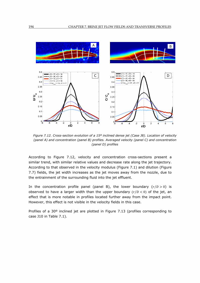
194 CHAPTER 7. BRINE JET FLOW FIELDS AND TRANSVERSE PROFILES
According to Figure 7.12, velocity and concentration cross-sections present a
similar trend, with similar relative values and decrease rate along the jet trajectory.
According to that observed in the velocity modulus (Figure 7.1) and dilution (Figure
7.7) fields, the jet width increases as the jet moves away from the nozzle, due to
the entrainment of the surrounding fluid into the jet effluent.
In the concentration profile panel (panel B), the lower boundary ( ⁄ 0) is
observed to have a larger width than the upper boundary ⁄ 0 of the jet, an
effect that is more notable in profiles located further away from the impact point.
However, this effect is not visible in the velocity fields in this case.
Profiles of a 30º inclined jet are plotted in Figure 7.13 (profiles corresponding to
case J10 in Table 7.1).
A B
C D
Figure 7.12. Cross-section evolution of a 15º inclined dense jet (Case J8). Location of velocity (panel A) and concentration (panel B) profiles. Averaged velocity (panel C) and concentration
(panel D) profiles
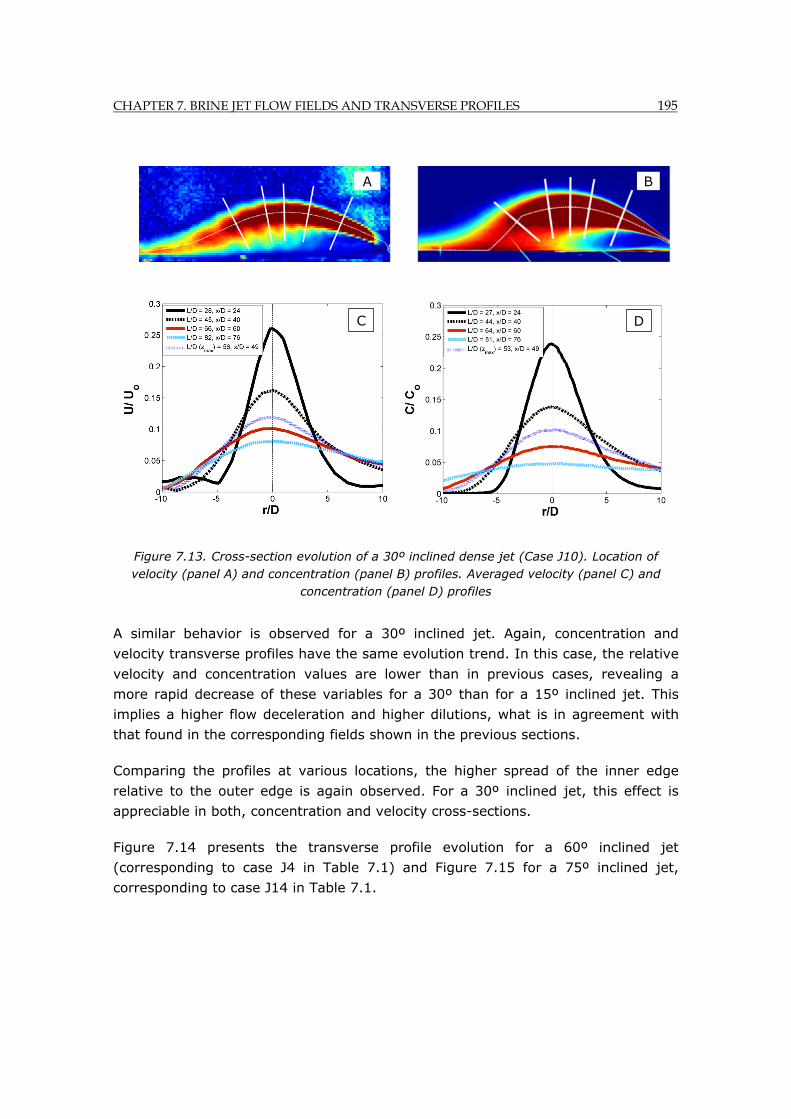
CHAPTER 7. BRINE JET FLOW FIELDS AND TRANSVERSE PROFILES 195
Figure 7.13. Cross-section evolution of a 30º inclined dense jet (Case J10). Location of velocity (panel A) and concentration (panel B) profiles. Averaged velocity (panel C) and
concentration (panel D) profiles
A similar behavior is observed for a 30º inclined jet. Again, concentration and
velocity transverse profiles have the same evolution trend. In this case, the relative
velocity and concentration values are lower than in previous cases, revealing a
more rapid decrease of these variables for a 30º than for a 15º inclined jet. This
implies a higher flow deceleration and higher dilutions, what is in agreement with
that found in the corresponding fields shown in the previous sections.
Comparing the profiles at various locations, the higher spread of the inner edge
relative to the outer edge is again observed. For a 30º inclined jet, this effect is
appreciable in both, concentration and velocity cross-sections.
Figure 7.14 presents the transverse profile evolution for a 60º inclined jet
(corresponding to case J4 in Table 7.1) and Figure 7.15 for a 75º inclined jet,
corresponding to case J14 in Table 7.1.
A B
C D
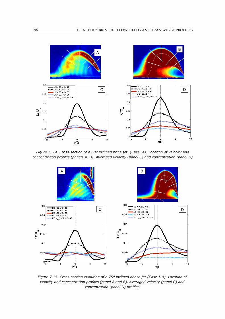
196 CHAPTER 7. BRINE JET FLOW FIELDS AND TRANSVERSE PROFILES
Figure 7. 14. Cross-section of a 60º inclined brine jet. (Case J4). Location of velocity and concentration profiles (panels A, B). Averaged velocity (panel C) and concentration (panel D)
A B
C D
A B
D C
Figure 7.15. Cross-section evolution of a 75º inclined dense jet (Case J14). Location of velocity and concentration profiles (panel A and B). Averaged velocity (panel C) and
concentration (panel D) profiles
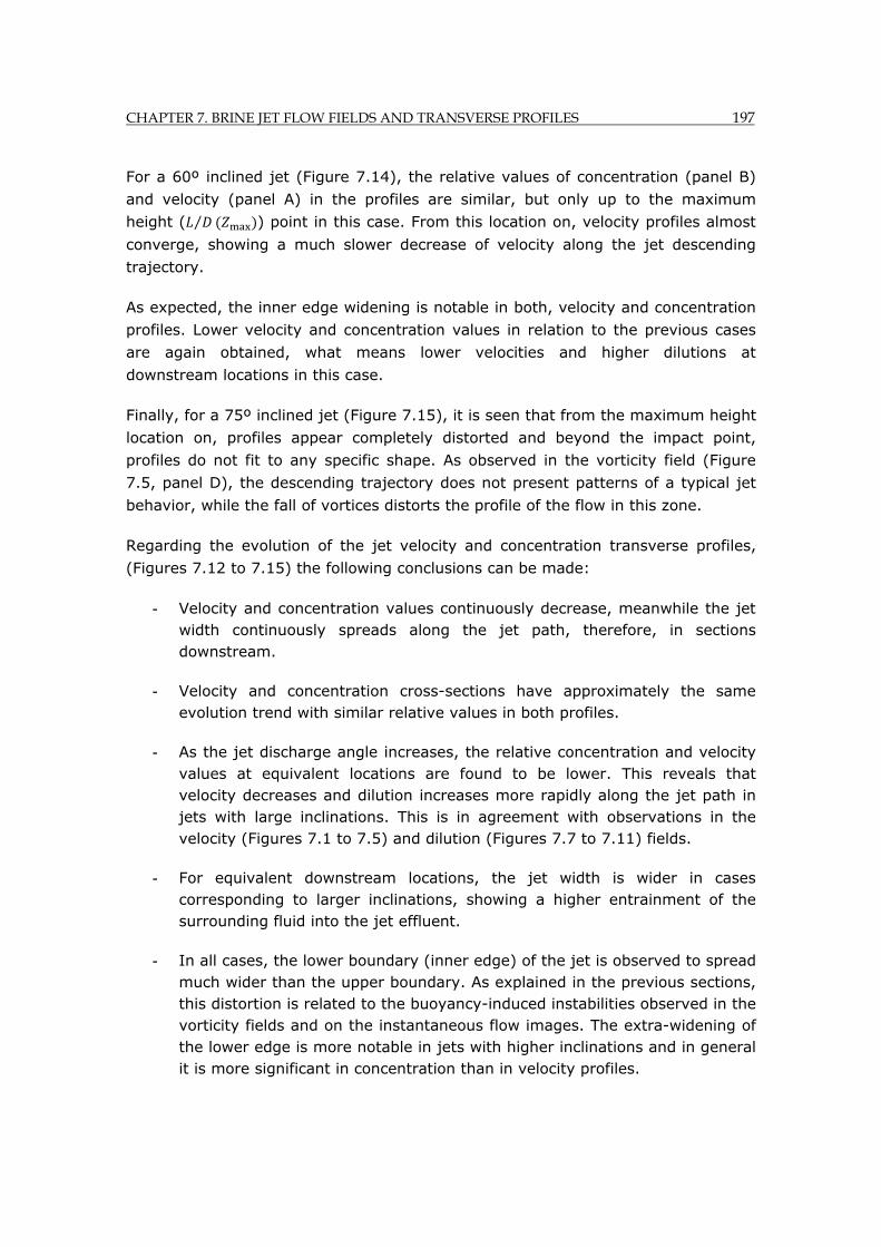
CHAPTER 7. BRINE JET FLOW FIELDS AND TRANSVERSE PROFILES 197
For a 60º inclined jet (Figure 7.14), the relative values of concentration (panel B)
and velocity (panel A) in the profiles are similar, but only up to the maximum
height ( ⁄ ) point in this case. From this location on, velocity profiles almost
converge, showing a much slower decrease of velocity along the jet descending
trajectory.
As expected, the inner edge widening is notable in both, velocity and concentration
profiles. Lower velocity and concentration values in relation to the previous cases
are again obtained, what means lower velocities and higher dilutions at
downstream locations in this case.
Finally, for a 75º inclined jet (Figure 7.15), it is seen that from the maximum height
location on, profiles appear completely distorted and beyond the impact point,
profiles do not fit to any specific shape. As observed in the vorticity field (Figure
7.5, panel D), the descending trajectory does not present patterns of a typical jet
behavior, while the fall of vortices distorts the profile of the flow in this zone.
Regarding the evolution of the jet velocity and concentration transverse profiles,
(Figures 7.12 to 7.15) the following conclusions can be made:
- Velocity and concentration values continuously decrease, meanwhile the jet width continuously spreads along the jet path, therefore, in sections downstream.
- Velocity and concentration cross-sections have approximately the same evolution trend with similar relative values in both profiles.
- As the jet discharge angle increases, the relative concentration and velocity values at equivalent locations are found to be lower. This reveals that velocity decreases and dilution increases more rapidly along the jet path in jets with large inclinations. This is in agreement with observations in the velocity (Figures 7.1 to 7.5) and dilution (Figures 7.7 to 7.11) fields.
- For equivalent downstream locations, the jet width is wider in cases corresponding to larger inclinations, showing a higher entrainment of the surrounding fluid into the jet effluent.
- In all cases, the lower boundary (inner edge) of the jet is observed to spread much wider than the upper boundary. As explained in the previous sections, this distortion is related to the buoyancy-induced instabilities observed in the vorticity fields and on the instantaneous flow images. The extra-widening of the lower edge is more notable in jets with higher inclinations and in general it is more significant in concentration than in velocity profiles.
198 CHAPTER 7. BRINE JET FLOW FIELDS AND TRANSVERSE PROFILES
- For 75º inclined jets, velocity profiles appear totally distorted beyond the maximum height location.
To our knowledge, the cross-section analysis presented here is the first published which covers the full range of actual jet discharge angles and the characterization of the velocity and concentration transverse profiles along the full jet trajectory for all cases.
7.3.2. Nondimensional transverse profiles. Assessment of the self similarity and Gaussian profile hypothesis
In order to study the cross-section self-similarity assumption reliability, the jet
transverse profiles have been non-dimensionalized and plotted in Figures 7.16 to
7.19. The Velocity modulus ( ) and the corresponding horizontal ( ) and vertical
( ) components have been non-dimensionalized with the centerline velocity ( ),
whereas the averaged concentration profiles ( ) with the centerline concentration
( ).
Furthermore, to contrast the Gaussian profile hypothesis, generally assumed by jet
integral models, Gaussian curves corresponding to the following expressions,
Jirka (2004), have been obtained and plotted in the velocity and concentration
profile graphs:
⁄ 7.7
⁄ 7.8
Being 1.2, the dispersion rate for a pure jet or plume.
The profiles presented in Figures 7.16 to 7.19 correspond to the same locations
selected in the previous sections, again marked with white lines in the upper panels
(panels A and B) of the figures. The middle panels show the velocity modulus
(panel C) and the averaged concentration (panel D) profiles. Finally, the lower
panels show the horizontal (panel E) and the vertical (panel F) components of the
averaged velocity.
Locations are indicated in each profile by ⁄ and ⁄ distances from the nozzle.
Radial distances in profiles, , have been non-dimensionalized with the jet radii,
and . These values correspond to the radial distances from the centerline for
which velocity is 37% and concentration is 50% of centerline values, respectively.
The left middle side in profiles ( / 0) represents the jet upper boundary, while
the right side ( / 0), the lower edge. The x-axis shows radial distances at both
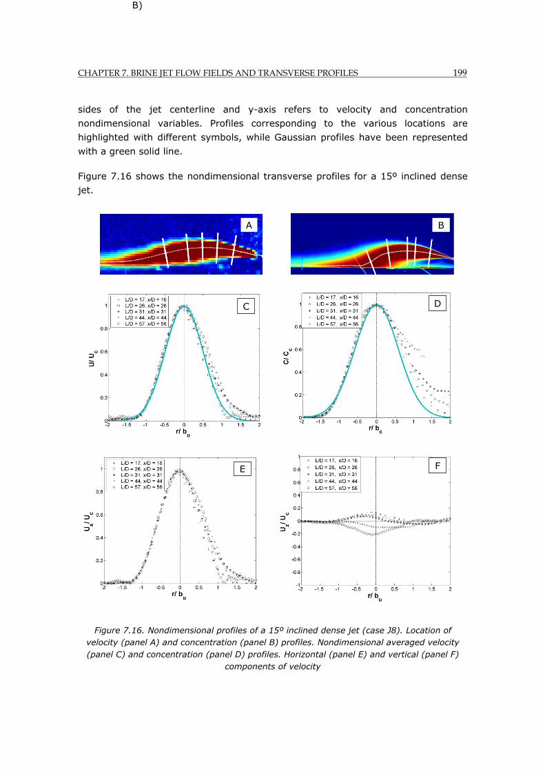
CHAPTER 7. BRINE JET FLOW FIELDS AND TRANSVERSE PROFILES 199
sides of the jet centerline and y-axis refers to velocity and concentration
nondimensional variables. Profiles corresponding to the various locations are
highlighted with different symbols, while Gaussian profiles have been represented
with a green solid line.
Figure 7.16 shows the nondimensional transverse profiles for a 15º inclined dense
jet.
Figure 7.16. Nondimensional profiles of a 15º inclined dense jet (case J8). Location of velocity (panel A) and concentration (panel B) profiles. Nondimensional averaged velocity (panel C) and concentration (panel D) profiles. Horizontal (panel E) and vertical (panel F)
components of velocity
B)
C D
F E
A B
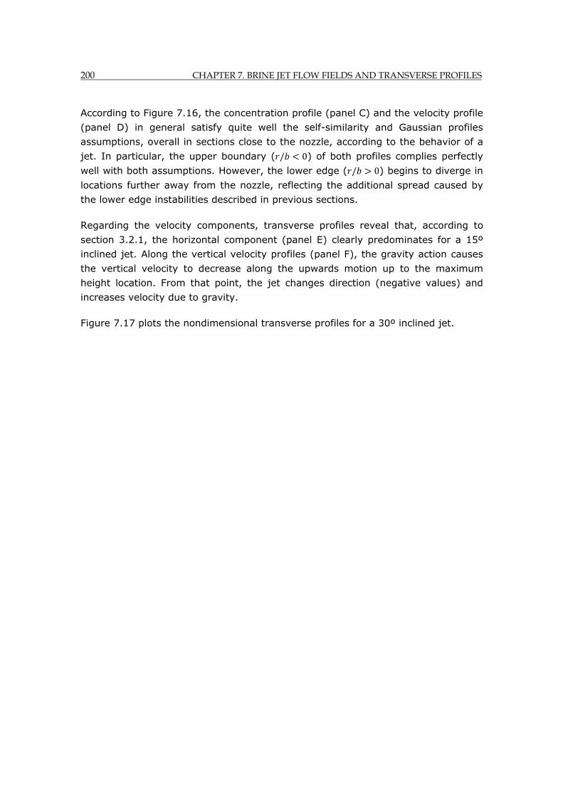
200 CHAPTER 7. BRINE JET FLOW FIELDS AND TRANSVERSE PROFILES
According to Figure 7.16, the concentration profile (panel C) and the velocity profile
(panel D) in general satisfy quite well the self-similarity and Gaussian profiles
assumptions, overall in sections close to the nozzle, according to the behavior of a
jet. In particular, the upper boundary ( / 0) of both profiles complies perfectly
well with both assumptions. However, the lower edge ( / 0) begins to diverge in
locations further away from the nozzle, reflecting the additional spread caused by
the lower edge instabilities described in previous sections.
Regarding the velocity components, transverse profiles reveal that, according to
section 3.2.1, the horizontal component (panel E) clearly predominates for a 15º
inclined jet. Along the vertical velocity profiles (panel F), the gravity action causes
the vertical velocity to decrease along the upwards motion up to the maximum
height location. From that point, the jet changes direction (negative values) and
increases velocity due to gravity.
Figure 7.17 plots the nondimensional transverse profiles for a 30º inclined jet.
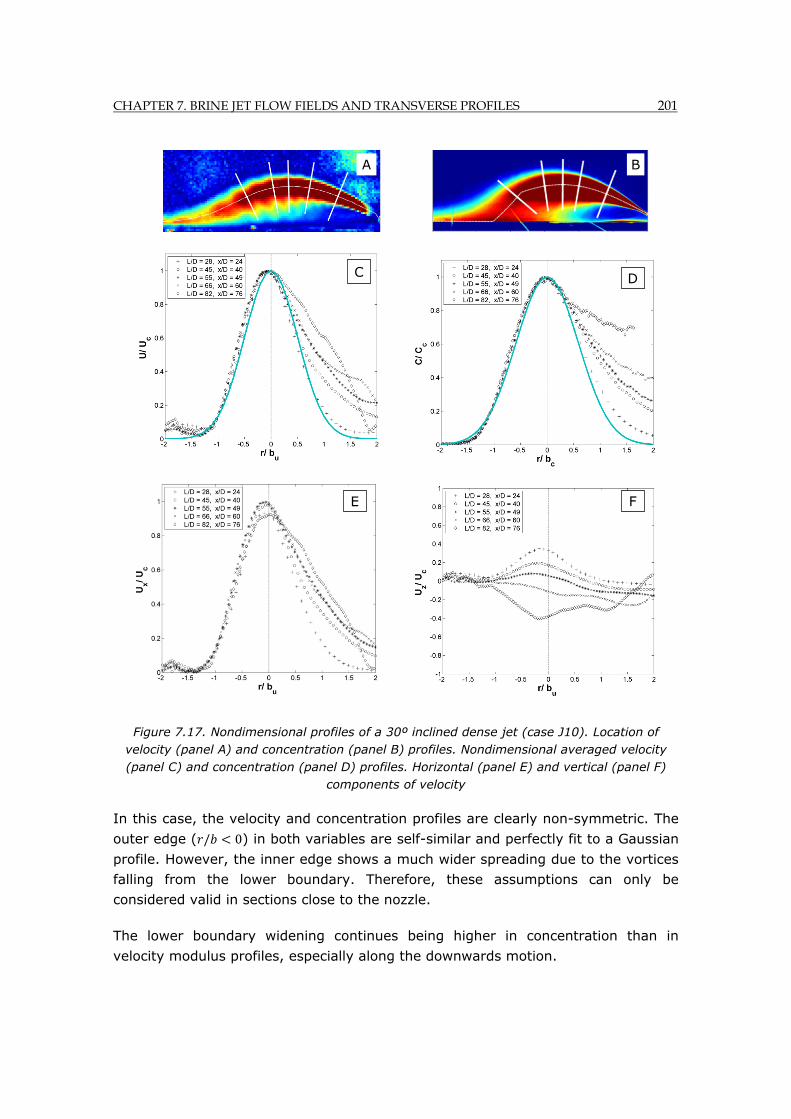
CHAPTER 7. BRINE JET FLOW FIELDS AND TRANSVERSE PROFILES 201
Figure 7.17. Nondimensional profiles of a 30º inclined dense jet (case J10). Location of velocity (panel A) and concentration (panel B) profiles. Nondimensional averaged velocity (panel C) and concentration (panel D) profiles. Horizontal (panel E) and vertical (panel F)
components of velocity
In this case, the velocity and concentration profiles are clearly non-symmetric. The
outer edge ( / 0) in both variables are self-similar and perfectly fit to a Gaussian
profile. However, the inner edge shows a much wider spreading due to the vortices
falling from the lower boundary. Therefore, these assumptions can only be
considered valid in sections close to the nozzle.
The lower boundary widening continues being higher in concentration than in
velocity modulus profiles, especially along the downwards motion.
A B
C
E
D
F
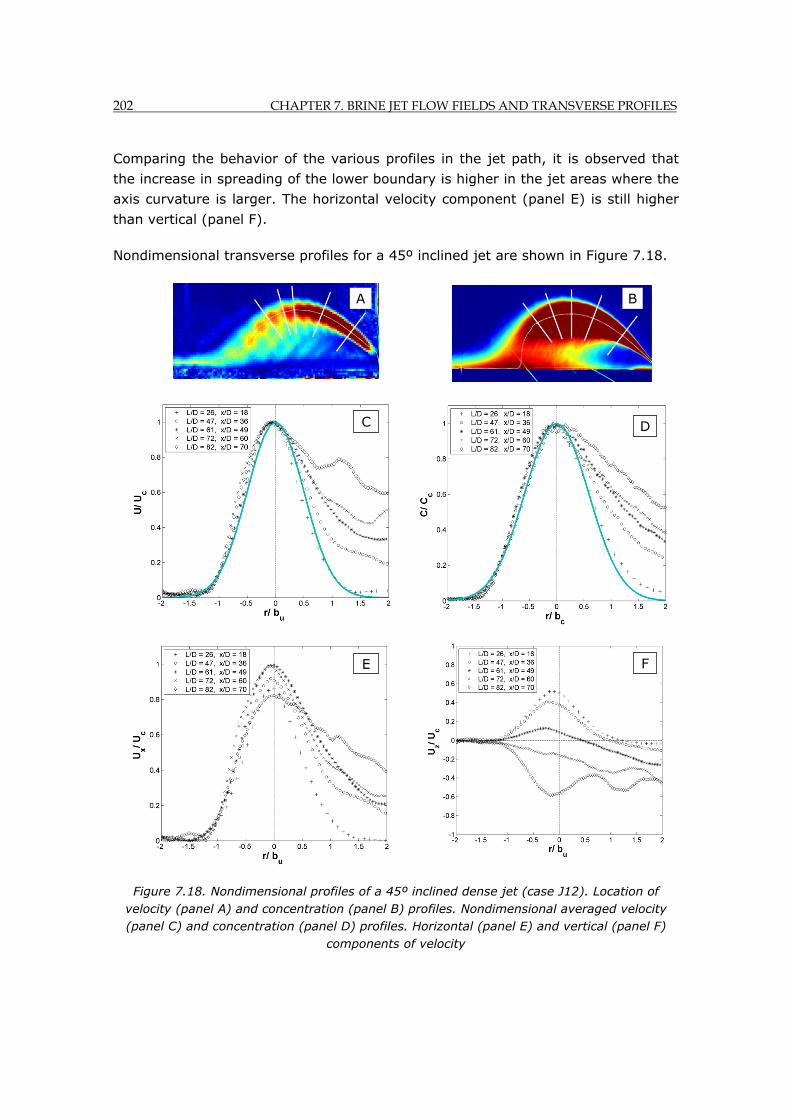
202 CHAPTER 7. BRINE JET FLOW FIELDS AND TRANSVERSE PROFILES
Comparing the behavior of the various profiles in the jet path, it is observed that
the increase in spreading of the lower boundary is higher in the jet areas where the
axis curvature is larger. The horizontal velocity component (panel E) is still higher
than vertical (panel F).
Nondimensional transverse profiles for a 45º inclined jet are shown in Figure 7.18.
Figure 7.18. Nondimensional profiles of a 45º inclined dense jet (case J12). Location of velocity (panel A) and concentration (panel B) profiles. Nondimensional averaged velocity (panel C) and concentration (panel D) profiles. Horizontal (panel E) and vertical (panel F)
components of velocity
A
C
E F
B
D

CHAPTER 7. BRINE JET FLOW FIELDS AND TRANSVERSE PROFILES 203
As has been shown, self-similarity and Gaussian profiles assumptions are only
reliable in the jet upper boundary, whereas the lower boundary diverges from these
assumptions. The inner edge spreading is observed to be more notable in sections
located in zones with a higher flow curvature, as in previous cases.
Although the vertical (panel F) and the horizontal (panel E) components of the
averaged velocity are identical at the jet nozzle, the vertical velocity decreases
more rapidly due to the combined effect of friction and gravity. As a consequence,
horizontal velocity is still higher in all sections. The transverse profile corresponding
to the locations furthest away from the nozzle, appears to be distorted in all
velocity panels. This deformation seems to be caused by the stable, coherent
structures observed in the velocity fields (Figure 7.3, panel A in Figure 7.18).
Figure 7.19 plots the nondimensional transverse profiles for a 75º inclined jet.
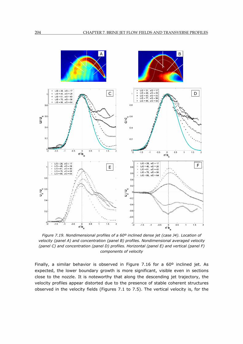
204 CHAPTER 7. BRINE JET FLOW FIELDS AND TRANSVERSE PROFILES
Figure 7.19. Nondimensional profiles of a 60º inclined dense jet (case J4). Location of velocity (panel A) and concentration (panel B) profiles. Nondimensional averaged velocity (panel C) and concentration (panel D) profiles. Horizontal (panel E) and vertical (panel F)
components of velocity
Finally, a similar behavior is observed in Figure 7.16 for a 60º inclined jet. As
expected, the lower boundary growth is more significant, visible even in sections
close to the nozzle. It is noteworthy that along the descending jet trajectory, the
velocity profiles appear distorted due to the presence of stable coherent structures
observed in the velocity fields (Figures 7.1 to 7.5). The vertical velocity is, for the
A
C
F
B
D
E

CHAPTER 7. BRINE JET FLOW FIELDS AND TRANSVERSE PROFILES 205
first time in the jets considered, predominant in the whole flow trajectory, except
for the maximum height zone.
For 75º inclined jets (not shown here), the large stable vortices, observed in
velocity fields, characterizing the descending jet trajectory make the adjustment of
profiles to any specific shape impossible.
In Kikkert et al. (2007) the averaged concentration profiles for a 30º, 45º and 60º
are presented and similar results are obtained. In that work, it is said that the
lower edge distortion increases with distance until the maximum height and beyond
that location, the profiles tend to collapse. However, in the present work, this trend
has not been found and the lower edge widening has been observed to continuously
increase along the full jet path. A particular feature found is that in profiles located
in the zones of the jet with a smaller curvature (particularly the zone of maximum
height), the distortion increases in a significantly lower rate, making the profiles at
these zones to almost converge.
The following conclusions can be made from the analysis carried out in this section:
- The upper jet boundary fits well with the self-similarity and Gaussian profile assumptions in concentration and velocity profile for all the angles considered, showing a behavior typical of jets in that boundary. For jets with a very large inclination (75º), where profiles appear distorted beyond the maximum centerline peak point and do not converge to any specific shape.
- From a certain distance from the nozzle, velocity and concentration profiles become non-symmetric, with a larger expansion of the lower boundary relative to the upper boundary. As a consequence, self-similarity and Gaussian profiles assumptions can only be considered well-preserved for cross-sections close to the jet nozzle, being non-valid in most of the jet trajectory. This profiles distortion is more evident and appears closer to the nozzle in dense jets with higher discharge angles.
- The lower edge extra-widening causing jet transverse profiles asymmetry is caused by buoyancy-driven instabilities, which are reflected in counterclockwise vortices falling down vertically from the jet lower edge, as clearly observed in the vorticity flow-fields and the snapshot flow images (Figures 7.1 to 7.5). This special feature is expected to increase the mixing and dilution of the surrounding fluid into the brine effluent.
- The brine jet profile distortion invalidated the self-similarity and Gaussian profile hypotheses generally assumed by integral models for this type of flow (i.e. CorJet of Cormix models or UM3 of Visual Plumes model). The
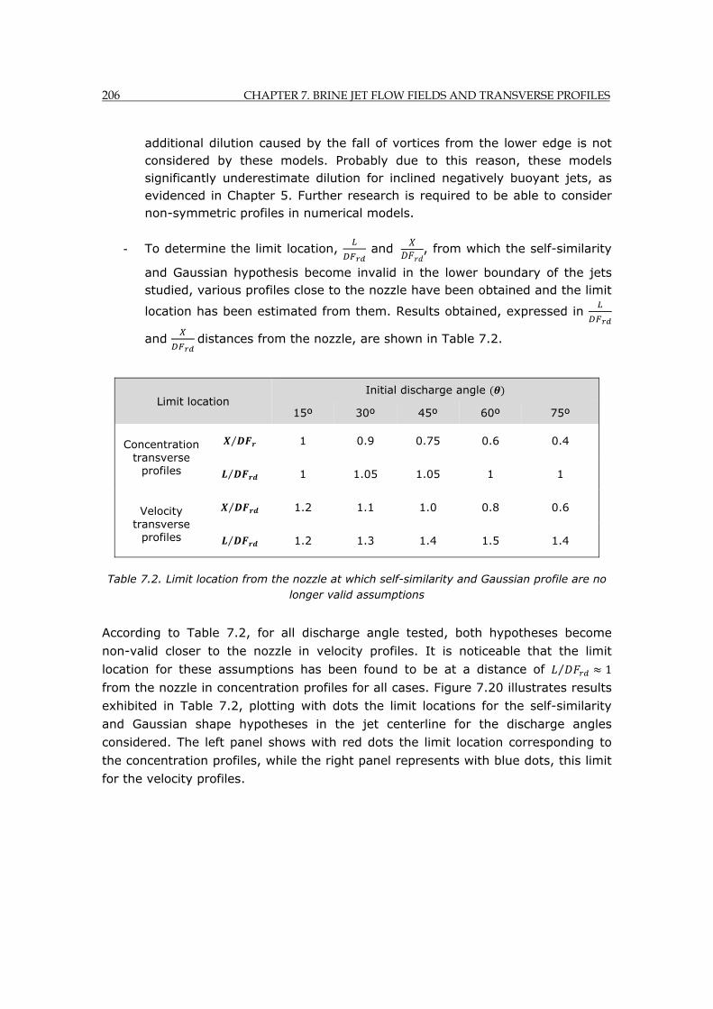
206 CHAPTER 7. BRINE JET FLOW FIELDS AND TRANSVERSE PROFILES
additional dilution caused by the fall of vortices from the lower edge is not considered by these models. Probably due to this reason, these models significantly underestimate dilution for inclined negatively buoyant jets, as evidenced in Chapter 5. Further research is required to be able to consider non-symmetric profiles in numerical models.
- To determine the limit location, and , from which the self-similarity
and Gaussian hypothesis become invalid in the lower boundary of the jets studied, various profiles close to the nozzle have been obtained and the limit
location has been estimated from them. Results obtained, expressed in
and distances from the nozzle, are shown in Table 7.2.
Table 7.2. Limit location from the nozzle at which self-similarity and Gaussian profile are no longer valid assumptions
According to Table 7.2, for all discharge angle tested, both hypotheses become
non-valid closer to the nozzle in velocity profiles. It is noticeable that the limit
location for these assumptions has been found to be at a distance of 1⁄
from the nozzle in concentration profiles for all cases. Figure 7.20 illustrates results
exhibited in Table 7.2, plotting with dots the limit locations for the self-similarity
and Gaussian shape hypotheses in the jet centerline for the discharge angles
considered. The left panel shows with red dots the limit location corresponding to
the concentration profiles, while the right panel represents with blue dots, this limit
for the velocity profiles.
Limit location Initial discharge angle
15º 30º 45º 60º 75º
Concentration transverse
profiles
⁄ 1 0.9 0.75 0.6 0.4
⁄ 1 1.05 1.05 1 1
Velocity transverse
profiles
⁄ 1.2 1.1 1.0 0.8 0.6
⁄ 1.2 1.3 1.4 1.5 1.4
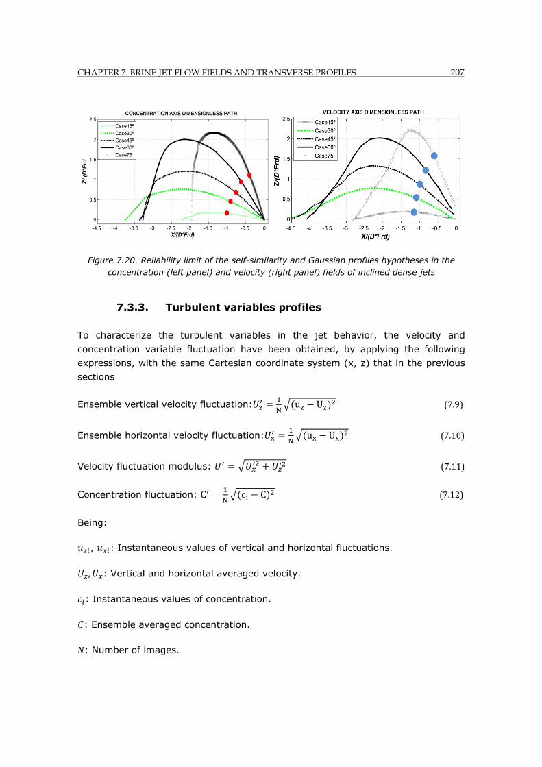
CHAPTER 7. BRINE JET FLOW FIELDS AND TRANSVERSE PROFILES 207
Figure 7.20. Reliability limit of the self-similarity and Gaussian profiles hypotheses in the concentration (left panel) and velocity (right panel) fields of inclined dense jets
7.3.3. Turbulent variables profiles
To characterize the turbulent variables in the jet behavior, the velocity and
concentration variable fluctuation have been obtained, by applying the following
expressions, with the same Cartesian coordinate system (x, z) that in the previous
sections
Ensemble vertical velocity fluctuation:N
u U (7.9)
Ensemble horizontal velocity fluctuation:N
u U (7.10)
Velocity fluctuation modulus: (7.11)
Concentration fluctuation: CN
c C (7.12)
Being:
, : Instantaneous values of vertical and horizontal fluctuations.
, : Vertical and horizontal averaged velocity.
: Instantaneous values of concentration.
: Ensemble averaged concentration.
: Number of images.
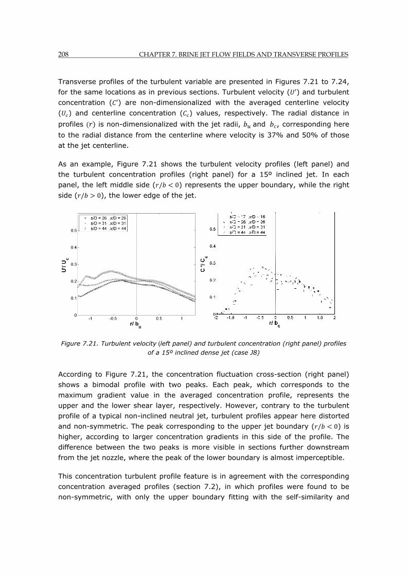
208 CHAPTER 7. BRINE JET FLOW FIELDS AND TRANSVERSE PROFILES
Transverse profiles of the turbulent variable are presented in Figures 7.21 to 7.24,
for the same locations as in previous sections. Turbulent velocity ( ) and turbulent
concentration ( ) are non-dimensionalized with the averaged centerline velocity
( ) and centerline concentration ( ) values, respectively. The radial distance in
profiles is non-dimensionalized with the jet radii, and , corresponding here
to the radial distance from the centerline where velocity is 37% and 50% of those
at the jet centerline.
As an example, Figure 7.21 shows the turbulent velocity profiles (left panel) and
the turbulent concentration profiles (right panel) for a 15º inclined jet. In each
panel, the left middle side ( / 0) represents the upper boundary, while the right
side ( / 0), the lower edge of the jet.
Figure 7.21. Turbulent velocity (left panel) and turbulent concentration (right panel) profiles of a 15º inclined dense jet (case J8)
According to Figure 7.21, the concentration fluctuation cross-section (right panel)
shows a bimodal profile with two peaks. Each peak, which corresponds to the
maximum gradient value in the averaged concentration profile, represents the
upper and the lower shear layer, respectively. However, contrary to the turbulent
profile of a typical non-inclined neutral jet, turbulent profiles appear here distorted
and non-symmetric. The peak corresponding to the upper jet boundary ( / 0) is
higher, according to larger concentration gradients in this side of the profile. The
difference between the two peaks is more visible in sections further downstream
from the jet nozzle, where the peak of the lower boundary is almost imperceptible.
This concentration turbulent profile feature is in agreement with the corresponding
concentration averaged profiles (section 7.2), in which profiles were found to be
non-symmetric, with only the upper boundary fitting with the self-similarity and
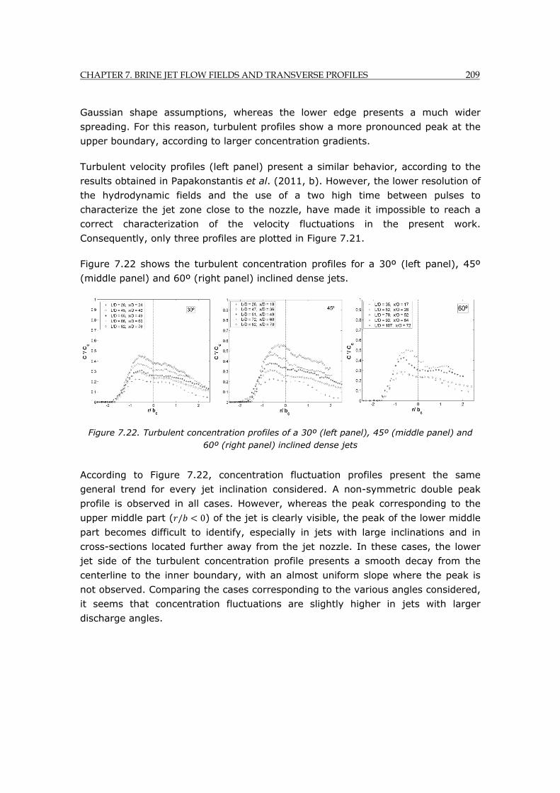
CHAPTER 7. BRINE JET FLOW FIELDS AND TRANSVERSE PROFILES 209
Gaussian shape assumptions, whereas the lower edge presents a much wider
spreading. For this reason, turbulent profiles show a more pronounced peak at the
upper boundary, according to larger concentration gradients.
Turbulent velocity profiles (left panel) present a similar behavior, according to the
results obtained in Papakonstantis et al. (2011, b). However, the lower resolution of
the hydrodynamic fields and the use of a two high time between pulses to
characterize the jet zone close to the nozzle, have made it impossible to reach a
correct characterization of the velocity fluctuations in the present work.
Consequently, only three profiles are plotted in Figure 7.21.
Figure 7.22 shows the turbulent concentration profiles for a 30º (left panel), 45º
(middle panel) and 60º (right panel) inclined dense jets.
Figure 7.22. Turbulent concentration profiles of a 30º (left panel), 45º (middle panel) and 60º (right panel) inclined dense jets
According to Figure 7.22, concentration fluctuation profiles present the same
general trend for every jet inclination considered. A non-symmetric double peak
profile is observed in all cases. However, whereas the peak corresponding to the
upper middle part ( / 0) of the jet is clearly visible, the peak of the lower middle
part becomes difficult to identify, especially in jets with large inclinations and in
cross-sections located further away from the jet nozzle. In these cases, the lower
jet side of the turbulent concentration profile presents a smooth decay from the
centerline to the inner boundary, with an almost uniform slope where the peak is
not observed. Comparing the cases corresponding to the various angles considered,
it seems that concentration fluctuations are slightly higher in jets with larger
discharge angles.
210 CHAPTER 7. BRINE JET FLOW FIELDS AND TRANSVERSE PROFILES
7.4. Conclusions
Based on the data obtained from a set of experiments carried out by non-intrusive
PIV and PLIF optical techniques, the present chapter and its companion (Chapter 7)
describe in detail the behavior of inclined hypersaline jets discharged into stagnant
environments.
In this chapter, the main flow-field characterizing the hydrodynamic and mixing
processes within the brine jet flow are characterized for different discharge angles.
Moreover, the averaged concentration and velocity nondimensional transverse
profiles have been analyzed, assessing the reliability degree of hypothesis assumed
by integral models, such as self-similarity and Gaussian shape cross-section. The
objective of the research is to go one-step further in the understanding of the
fundamental hydrodynamic and mixing processes of this type of inclined negatively
buoyant jets typical of brine discharges.
The following conclusions can be made from the study carried out:
- Hydrodynamic fields confirm that the horizontal momentum dominates the whole brine jet flow for 15º, 30º and 45º inclined jets, whereas the opposite happens for 60º and 75º inclined jets.
- In all cases, the horizontal momentum decreases smoothly from the nozzle to the impact point due to friction with the stagnant surrounding fluid. When the jet impacts the bottom, the total momentum turns into horizontal momentum and a dense horizontal layer (spreading layer) is formed. For 15º and 30º inclined jets, this dense layer moves overall forwards. However, for 60º and 75º inclined jets, the horizontal layer expands in all directions and, as a consequence, forward and backwards fluxes above the bottom are observed in the horizontal momentum fields. These fields also reveal the presence of coherent structures along the jet trajectory.
- The vertical component of momentum decreases from the nozzle to the maximum height location. In that point, it becomes zero and then it changes direction and the jet descends, increasing the vertical momentum due to gravitational acceleration. The vertical momentum has been observed to decrease always more rapidly than the horizontal counterpart along the ascending path, due to the combined effect of friction and the gravity force.
- In all cases, and especially in jets with a large inclination, the vertical momentum field shows a dispersed flow falling along the descending path, revealing a behavior closer to a buoyant plume than to a jet. Coherent
CHAPTER 7. BRINE JET FLOW FIELDS AND TRANSVERSE PROFILES 211
structures, increasing in size in locations further away from the nozzle, are observed in the vertical velocity fields, showing preferential channels within the flow. For 60º and 75º inclined jets, the downward trajectory and the preferential channels are observed to be almost vertical.
- The planar vorticity field reveals a behavior close to that of a pure jet along the ascending jet path in all cases. Indeed, a rotating clockwise flux is observed in the upper middle of the jet and a counterclockwise flux in the lower middle part, with zero vorticity equal to zero at the jet axis. However, along the descending brine jet path, this behavior typical of pure jets changes and while a counterclockwise flow is observed along the upper boundary, the lower boundary appears to be distorted, behaving closer to a plume flow. An interesting output from the vorticity field is the existence of counterclockwise vortices falling from the lower boundary along the full jet path. These vortices o buoyancy instabilities, especially notable in jets with a high discharge angle, are caused by the gravitational force, which makes the vortices to separate and fall vertically from the inclined dense jet lower edge. As a consequence, a swirl flow cascade and a dispersed flow typical of plumes, is observed in the snapshots images presented in this paper.
- Dilution continuously increases along the jet path, due to the entrainment of the surrounding fluid into the brine effluent trough the flow boundaries. As expected, the dilution rate is higher in jets with larger inclinations, whereas for jet with a very small discharge angle, such as 15º, the Coanda effect makes the jet to attach the bottom, significantly reducing dilution. In all cases, the dilution flow-fields reveal an unusual widening of the lower jet boundary, which spreads with a higher rate than the upper jet edge. This extra-widening is directly related to the fall of counterclockwise vortices previously explained and leads to higher dilutions along the jet lower boundary, which cannot be predicted by classic integral models.
- The analysis of nondimensional velocity and concentration cross-sections along the jet path reveals that the self-similarity and Gaussian profile assumptions in negatively buoyant inclined jets are only well satisfied in sections close to the jet nozzle. The limit location to assume these hypotheses has been found to be at a distance L⁄D≈1 from the jet nozzle in concentration profiles, and at a distance L⁄ D≈1.2~1.5 in velocity profiles.
- In cross-sections further away from the nozzle, whereas the upper boundary of the flow is in agreement with these assumptions, the lower middle part appears distorted due to the buoyancy-induced instabilities (fall of counterclockwise vortices from the lower edge) previously explained. As a

212 CHAPTER 7. BRINE JET FLOW FIELDS AND TRANSVERSE PROFILES
consequence non-symmetric concentration and velocity profiles are found for inclined brine jets, being higher this effect in jets with larger inclinations.
- The asymmetry detected in velocity and concentration profiles invalidated the self-similarity and Gaussian profile hypotheses in inclined negatively buoyant jets, such as those typical of brine jet discharges. Since this asymmetry notably affects flow behavior and dilution, significant errors are expected in numerical models assuming those hypotheses. That is the case of typical integral models, such as CORJET, UM3 and JETLAG, for which the dilution rate is significantly underestimated for this type of flow, as shown in Chapter 5.
- The analysis of cross-sections of turbulent variables shows a bimodal profile, with two peaks coinciding with the highest gradients in averaged variables (shear layer location). However, for inclined jets with a negative buoyancy this bimodal profile, contrary to profiles of pure jets, is non-symmetric, with a more pronounced peak in the upper middle than in the lower middle part of the brine jet. This feature is in agreement with the distorted averaged concentration and velocity profiles.
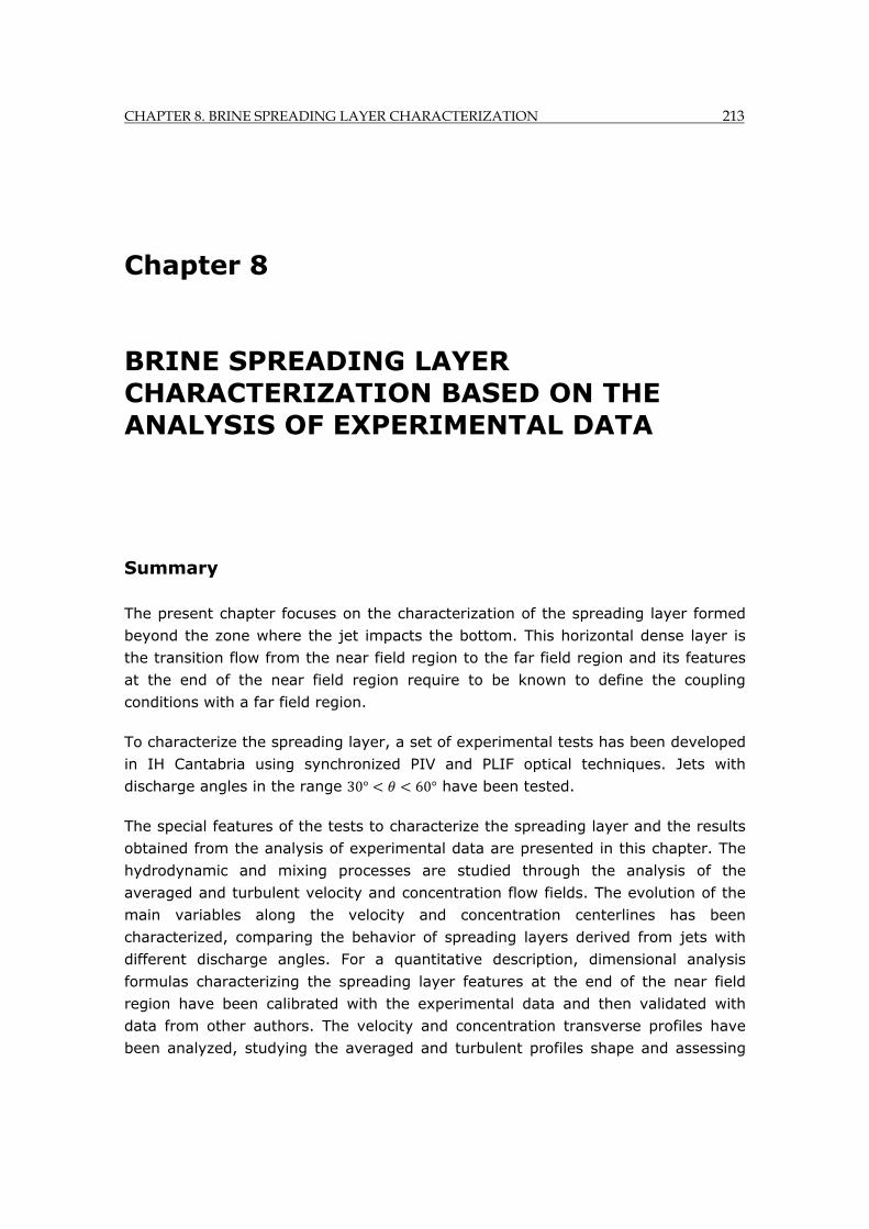
CHAPTER 8. BRINE SPREADING LAYER CHARACTERIZATION 213
Chapter 8. BRINE SPREADING LAYER CHARACTERIZATION BASED ON THE ANALYSIS OF EXPERIMENTAL DATA
Chapter 8 BRINE SPREADING LAYER CHARACTERIZATION BASED ON THE ANALYSIS OF EXPERIMENTAL DATA
Summary
The present chapter focuses on the characterization of the spreading layer formed
beyond the zone where the jet impacts the bottom. This horizontal dense layer is
the transition flow from the near field region to the far field region and its features
at the end of the near field region require to be known to define the coupling
conditions with a far field region.
To characterize the spreading layer, a set of experimental tests has been developed
in IH Cantabria using synchronized PIV and PLIF optical techniques. Jets with
discharge angles in the range 30° 60° have been tested.
The special features of the tests to characterize the spreading layer and the results
obtained from the analysis of experimental data are presented in this chapter. The
hydrodynamic and mixing processes are studied through the analysis of the
averaged and turbulent velocity and concentration flow fields. The evolution of the
main variables along the velocity and concentration centerlines has been
characterized, comparing the behavior of spreading layers derived from jets with
different discharge angles. For a quantitative description, dimensional analysis
formulas characterizing the spreading layer features at the end of the near field
region have been calibrated with the experimental data and then validated with
data from other authors. The velocity and concentration transverse profiles have
been analyzed, studying the averaged and turbulent profiles shape and assessing
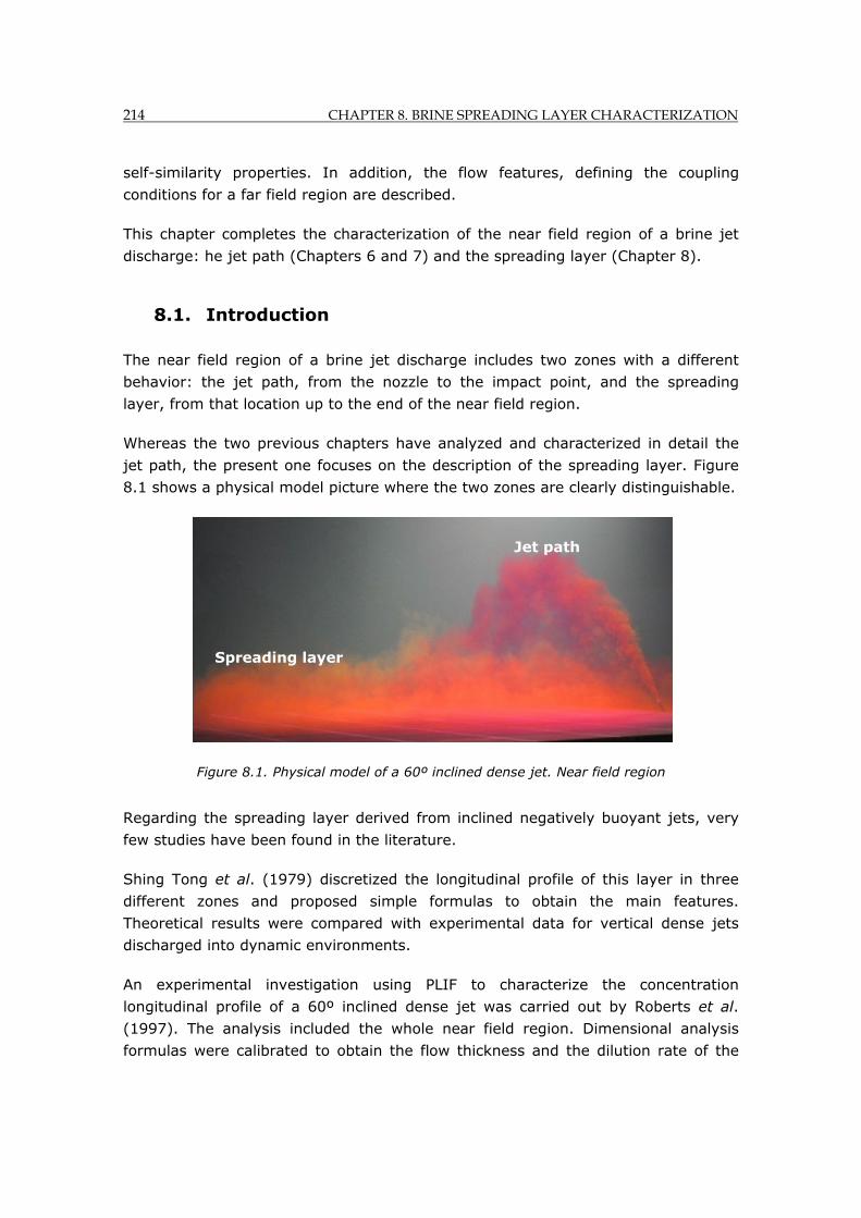
214 CHAPTER 8. BRINE SPREADING LAYER CHARACTERIZATION
self-similarity properties. In addition, the flow features, defining the coupling
conditions for a far field region are described.
This chapter completes the characterization of the near field region of a brine jet
discharge: he jet path (Chapters 6 and 7) and the spreading layer (Chapter 8).
8.1. Introduction
The near field region of a brine jet discharge includes two zones with a different
behavior: the jet path, from the nozzle to the impact point, and the spreading
layer, from that location up to the end of the near field region.
Whereas the two previous chapters have analyzed and characterized in detail the
jet path, the present one focuses on the description of the spreading layer. Figure
8.1 shows a physical model picture where the two zones are clearly distinguishable.
Figure 8.1. Physical model of a 60º inclined dense jet. Near field region
Regarding the spreading layer derived from inclined negatively buoyant jets, very
few studies have been found in the literature.
Shing Tong et al. (1979) discretized the longitudinal profile of this layer in three
different zones and proposed simple formulas to obtain the main features.
Theoretical results were compared with experimental data for vertical dense jets
discharged into dynamic environments.
An experimental investigation using PLIF to characterize the concentration
longitudinal profile of a 60º inclined dense jet was carried out by Roberts et al.
(1997). The analysis included the whole near field region. Dimensional analysis
formulas were calibrated to obtain the flow thickness and the dilution rate of the
Spreading layer
Jet path
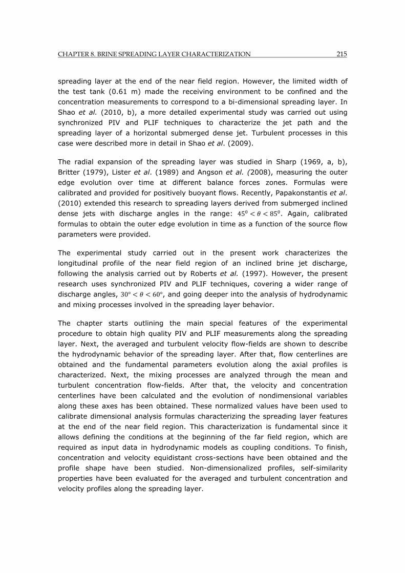
CHAPTER 8. BRINE SPREADING LAYER CHARACTERIZATION 215
spreading layer at the end of the near field region. However, the limited width of
the test tank (0.61 m) made the receiving environment to be confined and the
concentration measurements to correspond to a bi-dimensional spreading layer. In
Shao et al. (2010, b), a more detailed experimental study was carried out using
synchronized PIV and PLIF techniques to characterize the jet path and the
spreading layer of a horizontal submerged dense jet. Turbulent processes in this
case were described more in detail in Shao et al. (2009).
The radial expansion of the spreading layer was studied in Sharp (1969, a, b),
Britter (1979), Lister et al. (1989) and Angson et al. (2008), measuring the outer
edge evolution over time at different balance forces zones. Formulas were
calibrated and provided for positively buoyant flows. Recently, Papakonstantis et al.
(2010) extended this research to spreading layers derived from submerged inclined
dense jets with discharge angles in the range: 45 85 . Again, calibrated
formulas to obtain the outer edge evolution in time as a function of the source flow
parameters were provided.
The experimental study carried out in the present work characterizes the
longitudinal profile of the near field region of an inclined brine jet discharge,
following the analysis carried out by Roberts et al. (1997). However, the present
research uses synchronized PIV and PLIF techniques, covering a wider range of
discharge angles, 30° 60°, and going deeper into the analysis of hydrodynamic
and mixing processes involved in the spreading layer behavior.
The chapter starts outlining the main special features of the experimental
procedure to obtain high quality PIV and PLIF measurements along the spreading
layer. Next, the averaged and turbulent velocity flow-fields are shown to describe
the hydrodynamic behavior of the spreading layer. After that, flow centerlines are
obtained and the fundamental parameters evolution along the axial profiles is
characterized. Next, the mixing processes are analyzed through the mean and
turbulent concentration flow-fields. After that, the velocity and concentration
centerlines have been calculated and the evolution of nondimensional variables
along these axes has been obtained. These normalized values have been used to
calibrate dimensional analysis formulas characterizing the spreading layer features
at the end of the near field region. This characterization is fundamental since it
allows defining the conditions at the beginning of the far field region, which are
required as input data in hydrodynamic models as coupling conditions. To finish,
concentration and velocity equidistant cross-sections have been obtained and the
profile shape have been studied. Non-dimensionalized profiles, self-similarity
properties have been evaluated for the averaged and turbulent concentration and
velocity profiles along the spreading layer.
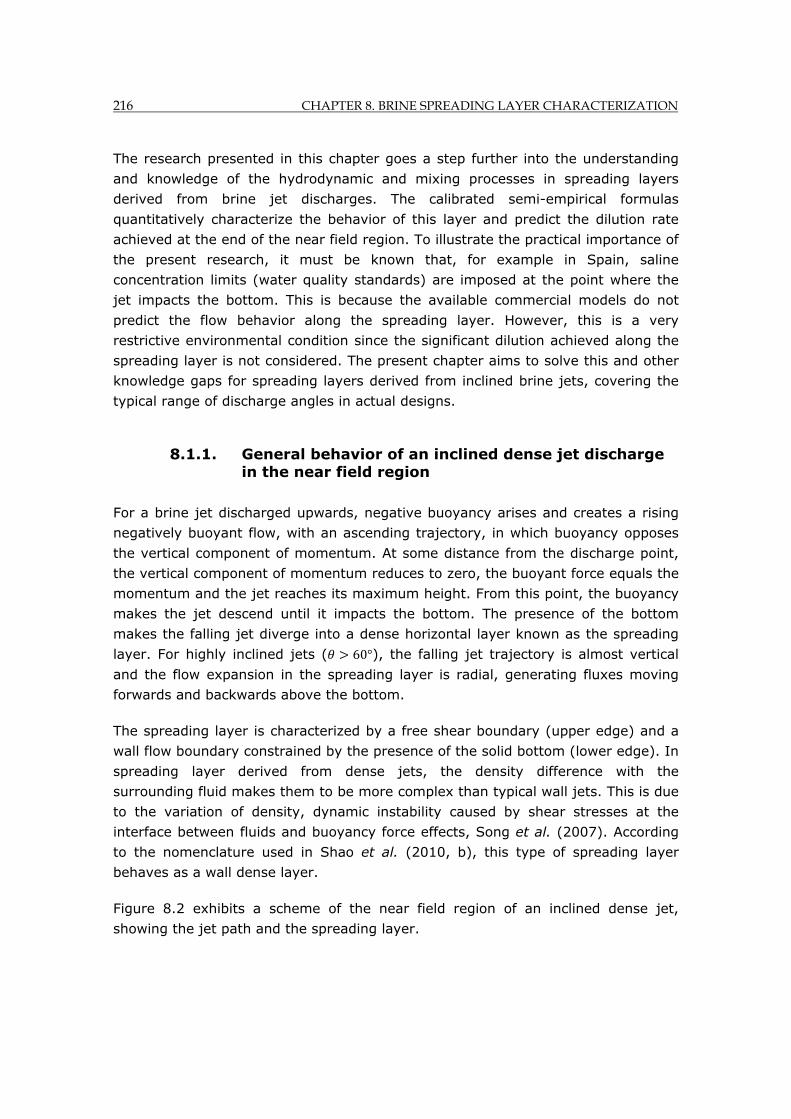
216 CHAPTER 8. BRINE SPREADING LAYER CHARACTERIZATION
The research presented in this chapter goes a step further into the understanding
and knowledge of the hydrodynamic and mixing processes in spreading layers
derived from brine jet discharges. The calibrated semi-empirical formulas
quantitatively characterize the behavior of this layer and predict the dilution rate
achieved at the end of the near field region. To illustrate the practical importance of
the present research, it must be known that, for example in Spain, saline
concentration limits (water quality standards) are imposed at the point where the
jet impacts the bottom. This is because the available commercial models do not
predict the flow behavior along the spreading layer. However, this is a very
restrictive environmental condition since the significant dilution achieved along the
spreading layer is not considered. The present chapter aims to solve this and other
knowledge gaps for spreading layers derived from inclined brine jets, covering the
typical range of discharge angles in actual designs.
8.1.1. General behavior of an inclined dense jet discharge in the near field region
For a brine jet discharged upwards, negative buoyancy arises and creates a rising
negatively buoyant flow, with an ascending trajectory, in which buoyancy opposes
the vertical component of momentum. At some distance from the discharge point,
the vertical component of momentum reduces to zero, the buoyant force equals the
momentum and the jet reaches its maximum height. From this point, the buoyancy
makes the jet descend until it impacts the bottom. The presence of the bottom
makes the falling jet diverge into a dense horizontal layer known as the spreading
layer. For highly inclined jets ( 60°), the falling jet trajectory is almost vertical
and the flow expansion in the spreading layer is radial, generating fluxes moving
forwards and backwards above the bottom.
The spreading layer is characterized by a free shear boundary (upper edge) and a
wall flow boundary constrained by the presence of the solid bottom (lower edge). In
spreading layer derived from dense jets, the density difference with the
surrounding fluid makes them to be more complex than typical wall jets. This is due
to the variation of density, dynamic instability caused by shear stresses at the
interface between fluids and buoyancy force effects, Song et al. (2007). According
to the nomenclature used in Shao et al. (2010, b), this type of spreading layer
behaves as a wall dense layer.
Figure 8.2 exhibits a scheme of the near field region of an inclined dense jet,
showing the jet path and the spreading layer.
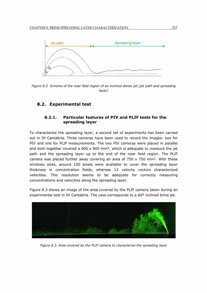
CHAPTER 8. BRINE SPREADING LAYER CHARACTERIZATION 217
Figure 8.2. Scheme of the near field region of an inclined dense jet (jet path and spreading layer)
8.2. Experimental test
8.2.1. Particular features of PIV and PLIF tests for the spreading layer
To characterize the spreading layer, a second set of experiments has been carried
out in IH Cantabria. Three cameras have been used to record the images: two for
PIV and one for PLIF measurements. The two PIV cameras were placed in parallel
and both together covered a 900 x 900 mm², which is adequate to measure the jet
path and the spreading layer up to the end of the near field region. The PLIF
camera was placed further away covering an area of 750 x 750 mm². With these
windows sizes, around 150 pixels were available to cover the spreading layer
thickness in concentration fields, whereas 12 velocity vectors characterized
velocities. This resolution seems to be adequate for correctly measuring
concentrations and velocities along the spreading layer.
Figure 8.3 shows an image of the area covered by the PLIF camera taken during an
experimental test in IH Cantabria. The case corresponds to a 60º inclined brine jet.
Figure 8.3. Area covered by the PLIF camera to characterize the spreading layer
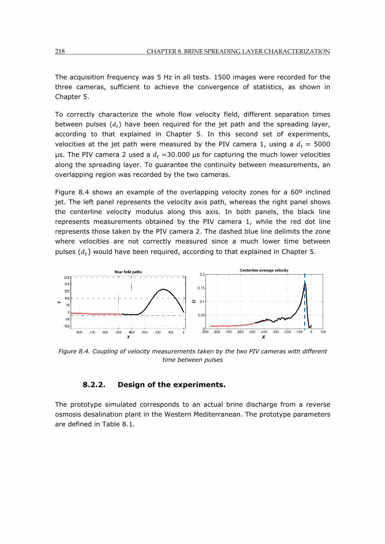
218 CHAPTER 8. BRINE SPREADING LAYER CHARACTERIZATION
The acquisition frequency was 5 Hz in all tests. 1500 images were recorded for the
three cameras, sufficient to achieve the convergence of statistics, as shown in
Chapter 5.
To correctly characterize the whole flow velocity field, different separation times
between pulses ( ) have been required for the jet path and the spreading layer,
according to that explained in Chapter 5. In this second set of experiments,
velocities at the jet path were measured by the PIV camera 1, using a 5000
µs. The PIV camera 2 used a 30.000 µs for capturing the much lower velocities
along the spreading layer. To guarantee the continuity between measurements, an
overlapping region was recorded by the two cameras.
Figure 8.4 shows an example of the overlapping velocity zones for a 60º inclined
jet. The left panel represents the velocity axis path, whereas the right panel shows
the centerline velocity modulus along this axis. In both panels, the black line
represents measurements obtained by the PIV camera 1, while the red dot line
represents those taken by the PIV camera 2. The dashed blue line delimits the zone
where velocities are not correctly measured since a much lower time between
pulses ( ) would have been required, according to that explained in Chapter 5.
Figure 8.4. Coupling of velocity measurements taken by the two PIV cameras with different time between pulses
8.2.2. Design of the experiments.
The prototype simulated corresponds to an actual brine discharge from a reverse
osmosis desalination plant in the Western Mediterranean. The prototype parameters
are defined in Table 8.1.

CHAPTER 8. BRINE SPREADING LAYER CHARACTERIZATION 219
PROTOTYPE SIMULATED
psu Psu Psu kg/m3 Kg/m3 Kg/m³ m m m/s º
37.5 68 30 1050 1026 22- 24 0.15 1 20 4 - 6 30º - 60º
Table 8.1. Design parameters of the prototype simulated to study the spreading layer
Being:
: Ambient salinity.
: Effluent saline concentration.
: Effluent density.
: Ambient density.
: Port diameter.
: Port height.
: Densimetric Froude number.
: Reduced gravity.
: Initial discharge velocity.
: Initial discharge angle.
Geometric and kinematic similarities are guaranteed by scaling magnitudes. The
scale was 1:50 in these experiments. The flow tested has a Reynolds number
higher than 2000, to ensure a fully developed turbulent jet flow. According to the
previous chapter, dynamic similarity is considered to be achieved, for a fully
developed turbulent flow, maintaining the same Densimetric Froude number at
prototype and model.
The saline concentration difference and the density difference between the effluent
and the receiving water fluid has been maintained at prototype and model test.
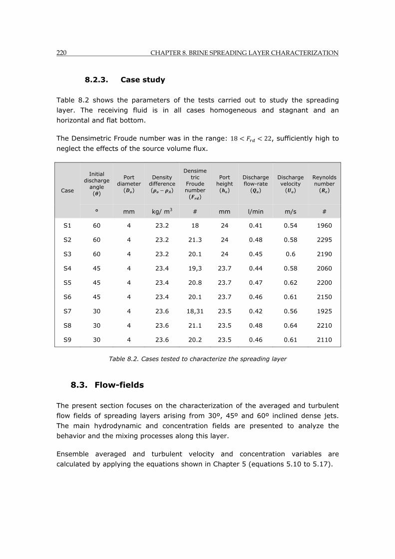
220 CHAPTER 8. BRINE SPREADING LAYER CHARACTERIZATION
8.2.3. Case study
Table 8.2 shows the parameters of the tests carried out to study the spreading
layer. The receiving fluid is in all cases homogeneous and stagnant and an
horizontal and flat bottom.
The Densimetric Froude number was in the range: 18 22, sufficiently high to
neglect the effects of the source volume flux.
Case
Initial discharge
angle ( )
Port diameter
( )
Density difference ( )
Densimetric
Froude number
( )
Port height ( )
Discharge flow-rate
( )
Discharge velocity
( )
Reynolds number
( )
° mm kg/ m3 # mm l/min m/s #
S1 60 4 23.2 18 24 0.41 0.54 1960
S2 60 4 23.2 21.3 24 0.48 0.58 2295
S3 60 4 23.2 20.1 24 0.45 0.6 2190
S4 45 4 23.4 19,3 23.7 0.44 0.58 2060
S5 45 4 23.4 20.8 23.7 0.47 0.62 2200
S6 45 4 23.4 20.1 23.7 0.46 0.61 2150
S7 30 4 23.6 18,31 23.5 0.42 0.56 1925
S8 30 4 23.6 21.1 23.5 0.48 0.64 2210
S9 30 4 23.6 20.2 23.5 0.46 0.61 2110
Table 8.2. Cases tested to characterize the spreading layer
8.3. Flow-fields
The present section focuses on the characterization of the averaged and turbulent
flow fields of spreading layers arising from 30º, 45º and 60º inclined dense jets.
The main hydrodynamic and concentration fields are presented to analyze the
behavior and the mixing processes along this layer.
Ensemble averaged and turbulent velocity and concentration variables are
calculated by applying the equations shown in Chapter 5 (equations 5.10 to 5.17).
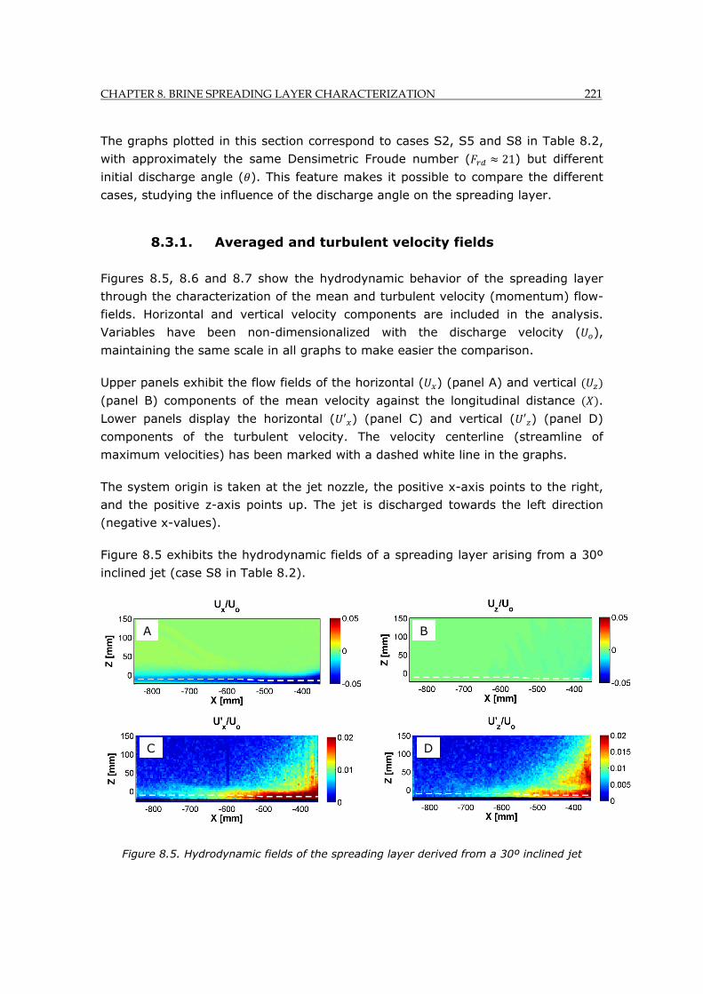
CHAPTER 8. BRINE SPREADING LAYER CHARACTERIZATION 221
The graphs plotted in this section correspond to cases S2, S5 and S8 in Table 8.2,
with approximately the same Densimetric Froude number ( 21) but different
initial discharge angle ( ). This feature makes it possible to compare the different
cases, studying the influence of the discharge angle on the spreading layer.
8.3.1. Averaged and turbulent velocity fields
Figures 8.5, 8.6 and 8.7 show the hydrodynamic behavior of the spreading layer
through the characterization of the mean and turbulent velocity (momentum) flow-
fields. Horizontal and vertical velocity components are included in the analysis.
Variables have been non-dimensionalized with the discharge velocity ( ),
maintaining the same scale in all graphs to make easier the comparison.
Upper panels exhibit the flow fields of the horizontal ( ) (panel A) and vertical
(panel B) components of the mean velocity against the longitudinal distance .
Lower panels display the horizontal ( ) (panel C) and vertical ( ) (panel D)
components of the turbulent velocity. The velocity centerline (streamline of
maximum velocities) has been marked with a dashed white line in the graphs.
The system origin is taken at the jet nozzle, the positive x-axis points to the right,
and the positive z-axis points up. The jet is discharged towards the left direction
(negative x-values).
Figure 8.5 exhibits the hydrodynamic fields of a spreading layer arising from a 30º
inclined jet (case S8 in Table 8.2).
Figure 8.5. Hydrodynamic fields of the spreading layer derived from a 30º inclined jet
A B
C D

222 CHAPTER 8. BRINE SPREADING LAYER CHARACTERIZATION
According to graphs of Figure 8.5, the horizontal averaged momentum (panel A) is
absolutely predominant along the spreading layer, being the value of the vertical
component (panel B) various orders of magnitude lower and hence, negligible.
As the spreading layer moves away from the impact point, the horizontal
momentum (panel A) diminishes due to bottom friction and the entrainment of the
surrounding fluid into the dense layer.
The bottom presence generates a boundary layer (wall-adjacent sub-layer), as
observed in panel A. The thickness of this boundary layer increases along the
spreading layer, causing a continuous upward displacement of the velocity axis.
The horizontal component of turbulent velocities (panel C) presents high values at
the first stretch of the spreading layer, of the same order of magnitude as the
corresponding horizontal averaged counterpart. As observed in this panel, velocity
fluctuations diminish along the spreading layer, revealing the collapse of turbulence
at the end of the near field region, where fluctuations are very low. According to
Song et al. (2007), the presence of the rigid boundary (bottom) reduces the length
scale of the fluctuations and increases the dissipation rate.
The vertical component of turbulent velocities (panel D) presents slightly lower
values and decreases more rapidly than the horizontal component (panel C). At the
end of the spreading layer, vertical turbulent velocities are close to zero.
Figure 8.6 shows the hydrodynamic fields of the spreading layer derived from a 45º
inclined dense jet (case S5 in Table 8.2).
Figure 8.6. Hydrodynamic fields of the spreading layer derived from a 45º inclined jet.
A B
C D
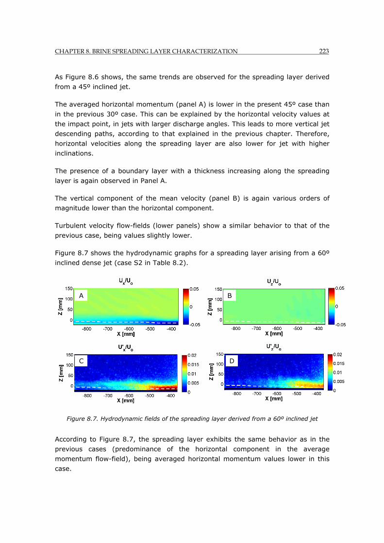
CHAPTER 8. BRINE SPREADING LAYER CHARACTERIZATION 223
As Figure 8.6 shows, the same trends are observed for the spreading layer derived
from a 45º inclined jet.
The averaged horizontal momentum (panel A) is lower in the present 45º case than
in the previous 30º case. This can be explained by the horizontal velocity values at
the impact point, in jets with larger discharge angles. This leads to more vertical jet
descending paths, according to that explained in the previous chapter. Therefore,
horizontal velocities along the spreading layer are also lower for jet with higher
inclinations.
The presence of a boundary layer with a thickness increasing along the spreading
layer is again observed in Panel A.
The vertical component of the mean velocity (panel B) is again various orders of
magnitude lower than the horizontal component.
Turbulent velocity flow-fields (lower panels) show a similar behavior to that of the
previous case, being values slightly lower.
Figure 8.7 shows the hydrodynamic graphs for a spreading layer arising from a 60º
inclined dense jet (case S2 in Table 8.2).
Figure 8.7. Hydrodynamic fields of the spreading layer derived from a 60º inclined jet
According to Figure 8.7, the spreading layer exhibits the same behavior as in the
previous cases (predominance of the horizontal component in the average
momentum flow-field), being averaged horizontal momentum values lower in this
case.
A B
C D
224 CHAPTER 8. BRINE SPREADING LAYER CHARACTERIZATION
Turbulent velocity (lower panels) presents lower values in this case as well. The
collapse of turbulence is evident at the end of the spreading layer in both, the
horizontal (panel C) and the vertical (panel D) components.
The following conclusions can be drawn from the analysis carried out in this
section:
- Momentum in the spreading layer is predominantly horizontal for all discharge angles studied, being vertical averaged velocities various orders of magnitude lower in all cases.
- The horizontal momentum diminishes along the spreading layer, due to bottom friction bottom and entrainment with the surrounding fluid.
- A boundary layer (wall adjacent sub-layer) above the bottom is observed in the averaged horizontal momentum. This layer is caused by the presence of the bottom. The layer thickness increases along the spreading layer, making the centerline velocity to slightly move upwards.
- Turbulent velocity values are higher in the zone close to the impact point, with values of the same order of magnitude as the averaged horizontal velocities. At locations downstream, fluctuations radically diminish, revealing the collapse of turbulence. At the end of the spreading layer, horizontal fluctuations are very low and vertical fluctuations are zero.
- Averaged horizontal velocities are observed to be higher in spreading layers derived from jets with lower discharge angles. This can be explained by lower horizontal velocities at the impact points in more inclined jets, which present more vertical descending jet trajectories.
8.3.2. Dilution fields
Figures 8.8, 8.9 and 8.10 show the flow-fields of net dilution and concentration
instantaneous images for brine discharges with various inclinations. These fields
have been analyzed for a better understanding of the mixing processes within the
flow, with special attention to the spreading layer.
The net dilution is obtained from the averaged concentration field by applying the
following expression to each pixel of the image.
C CAC CA
8.1
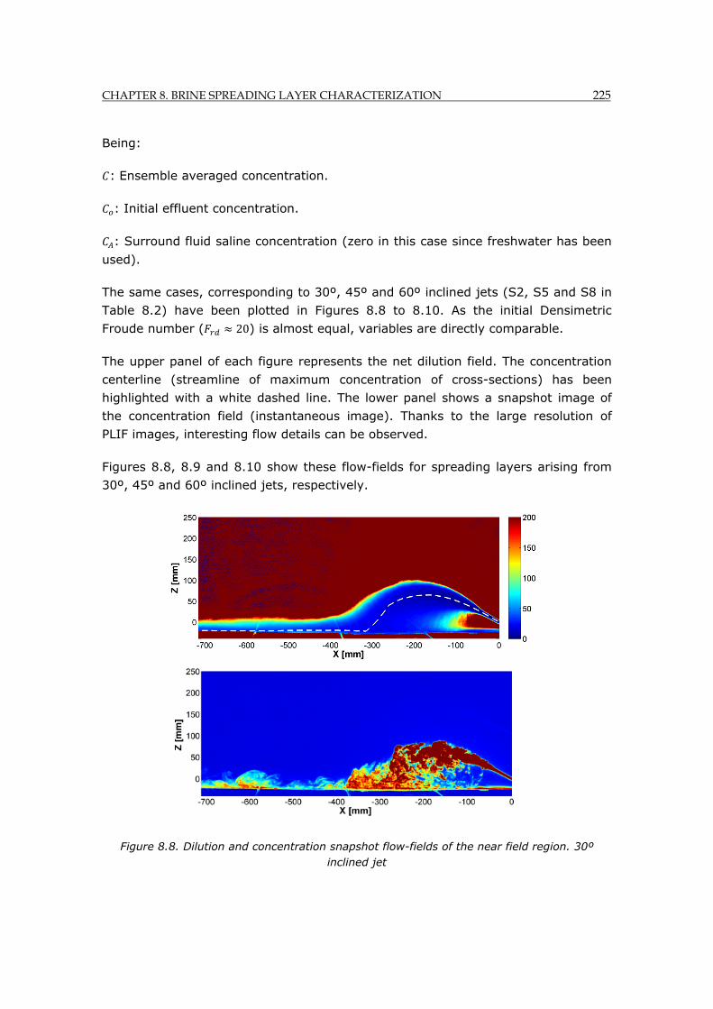
CHAPTER 8. BRINE SPREADING LAYER CHARACTERIZATION 225
Being:
: Ensemble averaged concentration.
: Initial effluent concentration.
: Surround fluid saline concentration (zero in this case since freshwater has been
used).
The same cases, corresponding to 30º, 45º and 60º inclined jets (S2, S5 and S8 in
Table 8.2) have been plotted in Figures 8.8 to 8.10. As the initial Densimetric
Froude number ( 20) is almost equal, variables are directly comparable.
The upper panel of each figure represents the net dilution field. The concentration
centerline (streamline of maximum concentration of cross-sections) has been
highlighted with a white dashed line. The lower panel shows a snapshot image of
the concentration field (instantaneous image). Thanks to the large resolution of
PLIF images, interesting flow details can be observed.
Figures 8.8, 8.9 and 8.10 show these flow-fields for spreading layers arising from
30º, 45º and 60º inclined jets, respectively.
Figure 8.8. Dilution and concentration snapshot flow-fields of the near field region. 30º inclined jet
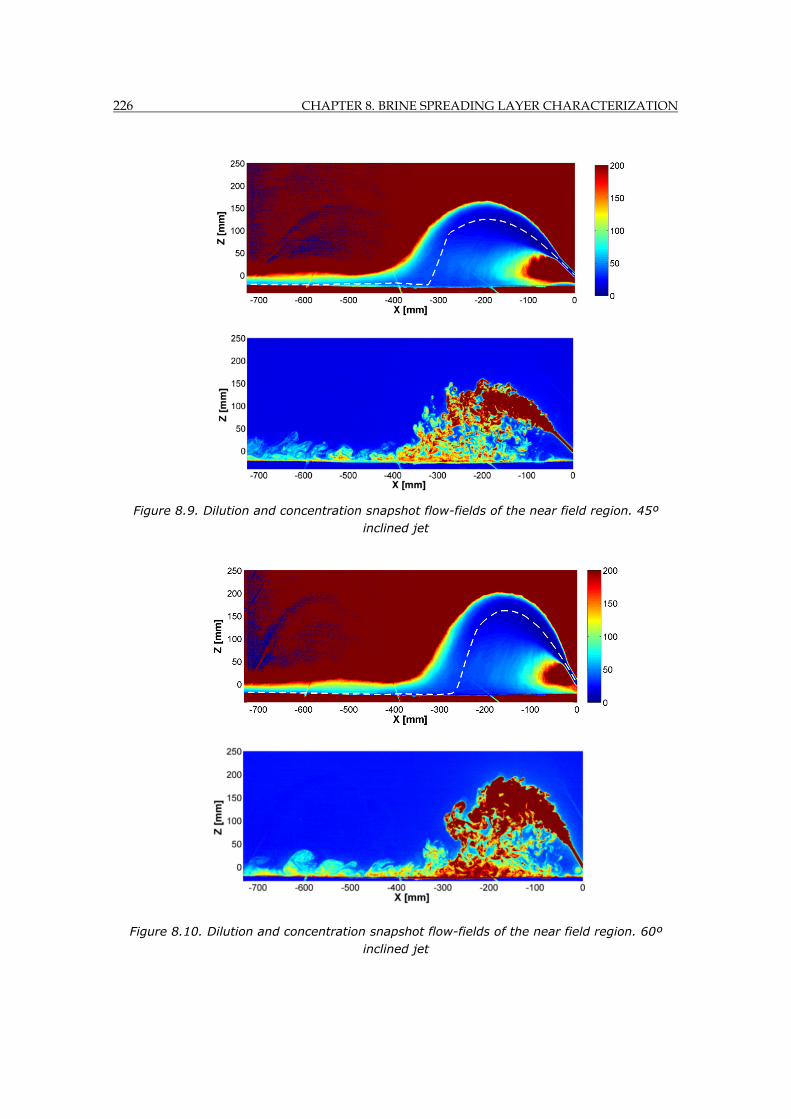
226 CHAPTER 8. BRINE SPREADING LAYER CHARACTERIZATION
Figure 8.9. Dilution and concentration snapshot flow-fields of the near field region. 45º inclined jet
Figure 8.10. Dilution and concentration snapshot flow-fields of the near field region. 60º inclined jet
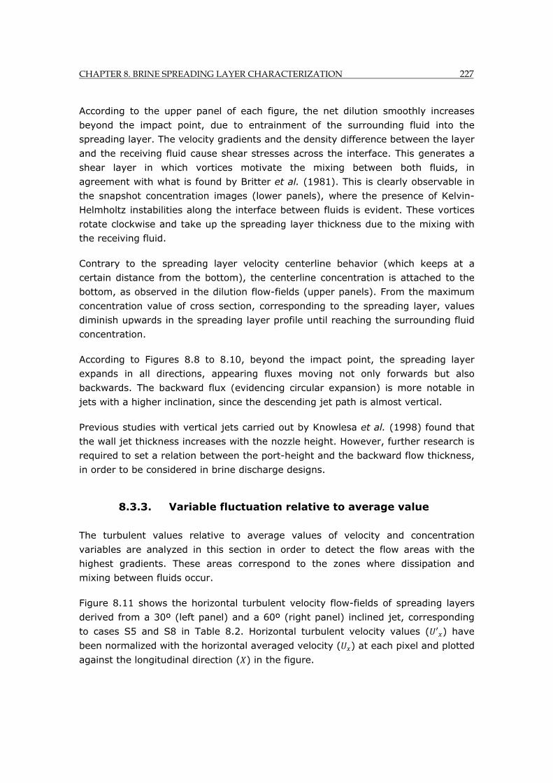
CHAPTER 8. BRINE SPREADING LAYER CHARACTERIZATION 227
According to the upper panel of each figure, the net dilution smoothly increases
beyond the impact point, due to entrainment of the surrounding fluid into the
spreading layer. The velocity gradients and the density difference between the layer
and the receiving fluid cause shear stresses across the interface. This generates a
shear layer in which vortices motivate the mixing between both fluids, in
agreement with what is found by Britter et al. (1981). This is clearly observable in
the snapshot concentration images (lower panels), where the presence of Kelvin-
Helmholtz instabilities along the interface between fluids is evident. These vortices
rotate clockwise and take up the spreading layer thickness due to the mixing with
the receiving fluid.
Contrary to the spreading layer velocity centerline behavior (which keeps at a
certain distance from the bottom), the centerline concentration is attached to the
bottom, as observed in the dilution flow-fields (upper panels). From the maximum
concentration value of cross section, corresponding to the spreading layer, values
diminish upwards in the spreading layer profile until reaching the surrounding fluid
concentration.
According to Figures 8.8 to 8.10, beyond the impact point, the spreading layer
expands in all directions, appearing fluxes moving not only forwards but also
backwards. The backward flux (evidencing circular expansion) is more notable in
jets with a higher inclination, since the descending jet path is almost vertical.
Previous studies with vertical jets carried out by Knowlesa et al. (1998) found that
the wall jet thickness increases with the nozzle height. However, further research is
required to set a relation between the port-height and the backward flow thickness,
in order to be considered in brine discharge designs.
8.3.3. Variable fluctuation relative to average value
The turbulent values relative to average values of velocity and concentration
variables are analyzed in this section in order to detect the flow areas with the
highest gradients. These areas correspond to the zones where dissipation and
mixing between fluids occur.
Figure 8.11 shows the horizontal turbulent velocity flow-fields of spreading layers
derived from a 30º (left panel) and a 60º (right panel) inclined jet, corresponding
to cases S5 and S8 in Table 8.2. Horizontal turbulent velocity values ( ) have
been normalized with the horizontal averaged velocity ( ) at each pixel and plotted
against the longitudinal direction ( ) in the figure.
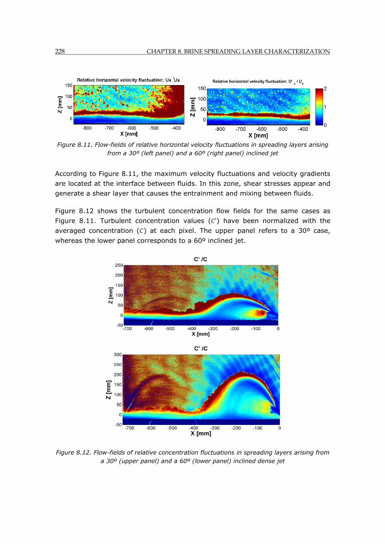
228 CHAPTER 8. BRINE SPREADING LAYER CHARACTERIZATION
Figure 8.11. Flow-fields of relative horizontal velocity fluctuations in spreading layers arising from a 30º (left panel) and a 60º (right panel) inclined jet
According to Figure 8.11, the maximum velocity fluctuations and velocity gradients
are located at the interface between fluids. In this zone, shear stresses appear and
generate a shear layer that causes the entrainment and mixing between fluids.
Figure 8.12 shows the turbulent concentration flow fields for the same cases as
Figure 8.11. Turbulent concentration values ( ) have been normalized with the
averaged concentration ( ) at each pixel. The upper panel refers to a 30º case,
whereas the lower panel corresponds to a 60º inclined jet.
Figure 8.12. Flow-fields of relative concentration fluctuations in spreading layers arising from a 30º (upper panel) and a 60º (lower panel) inclined dense jet
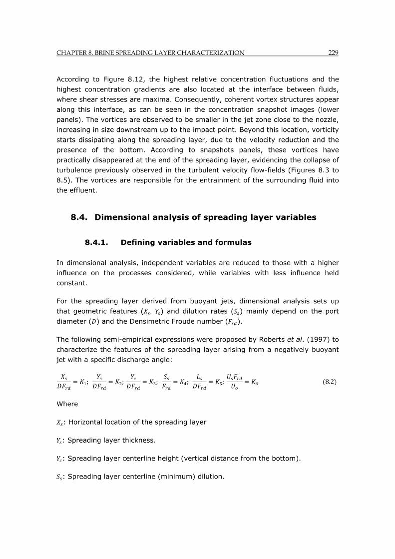
CHAPTER 8. BRINE SPREADING LAYER CHARACTERIZATION 229
According to Figure 8.12, the highest relative concentration fluctuations and the
highest concentration gradients are also located at the interface between fluids,
where shear stresses are maxima. Consequently, coherent vortex structures appear
along this interface, as can be seen in the concentration snapshot images (lower
panels). The vortices are observed to be smaller in the jet zone close to the nozzle,
increasing in size downstream up to the impact point. Beyond this location, vorticity
starts dissipating along the spreading layer, due to the velocity reduction and the
presence of the bottom. According to snapshots panels, these vortices have
practically disappeared at the end of the spreading layer, evidencing the collapse of
turbulence previously observed in the turbulent velocity flow-fields (Figures 8.3 to
8.5). The vortices are responsible for the entrainment of the surrounding fluid into
the effluent.
8.4. Dimensional analysis of spreading layer variables
8.4.1. Defining variables and formulas
In dimensional analysis, independent variables are reduced to those with a higher
influence on the processes considered, while variables with less influence held
constant.
For the spreading layer derived from buoyant jets, dimensional analysis sets up
that geometric features ( , ) and dilution rates ( ) mainly depend on the port
diameter ( ) and the Densimetric Froude number ( ).
The following semi-empirical expressions were proposed by Roberts et al. (1997) to
characterize the features of the spreading layer arising from a negatively buoyant
jet with a specific discharge angle:
; ; ; ; ; 8.2
Where
: Horizontal location of the spreading layer
: Spreading layer thickness.
: Spreading layer centerline height (vertical distance from the bottom).
: Spreading layer centerline (minimum) dilution.
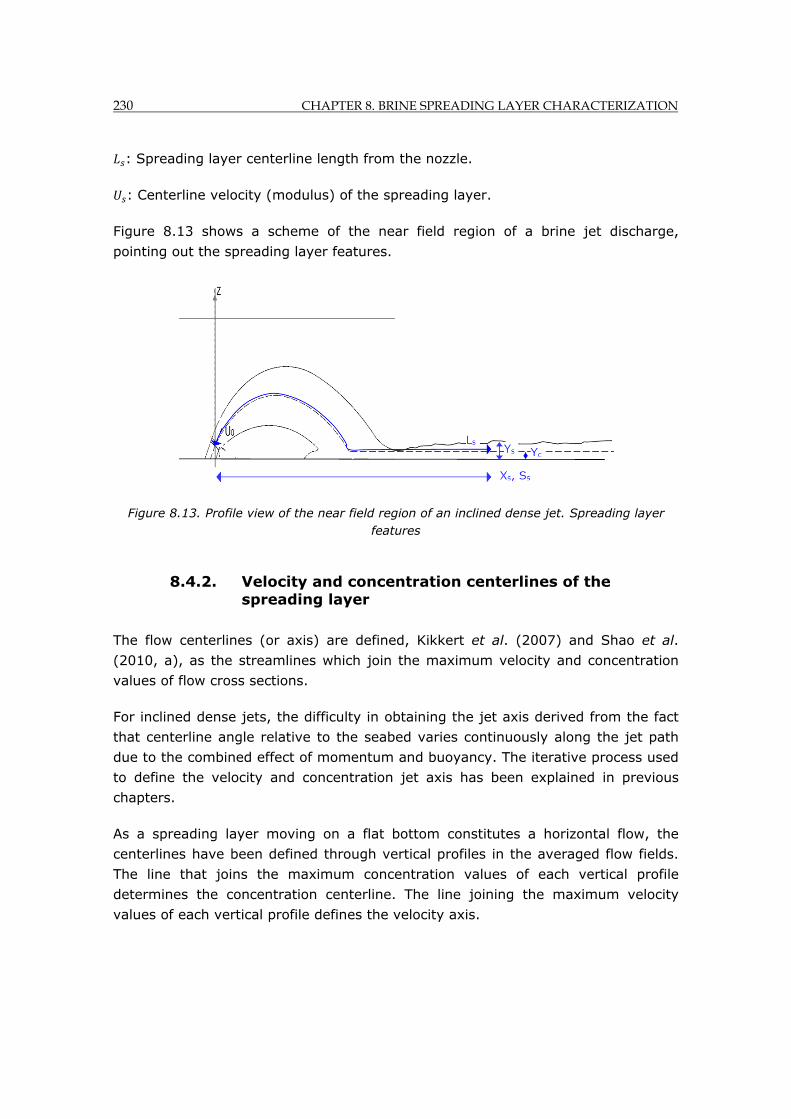
230 CHAPTER 8. BRINE SPREADING LAYER CHARACTERIZATION
: Spreading layer centerline length from the nozzle.
: Centerline velocity (modulus) of the spreading layer.
Figure 8.13 shows a scheme of the near field region of a brine jet discharge,
pointing out the spreading layer features.
Figure 8.13. Profile view of the near field region of an inclined dense jet. Spreading layer features
8.4.2. Velocity and concentration centerlines of the spreading layer
The flow centerlines (or axis) are defined, Kikkert et al. (2007) and Shao et al.
(2010, a), as the streamlines which join the maximum velocity and concentration
values of flow cross sections.
For inclined dense jets, the difficulty in obtaining the jet axis derived from the fact
that centerline angle relative to the seabed varies continuously along the jet path
due to the combined effect of momentum and buoyancy. The iterative process used
to define the velocity and concentration jet axis has been explained in previous
chapters.
As a spreading layer moving on a flat bottom constitutes a horizontal flow, the
centerlines have been defined through vertical profiles in the averaged flow fields.
The line that joins the maximum concentration values of each vertical profile
determines the concentration centerline. The line joining the maximum velocity
values of each vertical profile defines the velocity axis.
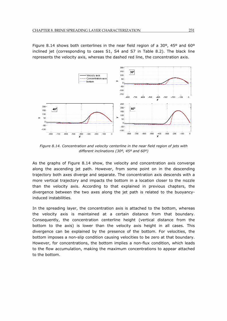
CHAPTER 8. BRINE SPREADING LAYER CHARACTERIZATION 231
Figure 8.14 shows both centerlines in the near field region of a 30º, 45º and 60º
inclined jet (corresponding to cases S1, S4 and S7 in Table 8.2). The black line
represents the velocity axis, whereas the dashed red line, the concentration axis.
Figure 8.14. Concentration and velocity centerline in the near field region of jets with different inclinations (30º, 45º and 60º)
As the graphs of Figure 8.14 show, the velocity and concentration axis converge
along the ascending jet path. However, from some point on in the descending
trajectory both axes diverge and separate. The concentration axis descends with a
more vertical trajectory and impacts the bottom in a location closer to the nozzle
than the velocity axis. According to that explained in previous chapters, the
divergence between the two axes along the jet path is related to the buoyancy-
induced instabilities.
In the spreading layer, the concentration axis is attached to the bottom, whereas
the velocity axis is maintained at a certain distance from that boundary.
Consequently, the concentration centerline height (vertical distance from the
bottom to the axis) is lower than the velocity axis height in all cases. This
divergence can be explained by the presence of the bottom. For velocities, the
bottom imposes a non-slip condition causing velocities to be zero at that boundary.
However, for concentrations, the bottom implies a non-flux condition, which leads
to the flow accumulation, making the maximum concentrations to appear attached
to the bottom.

232 CHAPTER 8. BRINE SPREADING LAYER CHARACTERIZATION
8.4.3. Evolution of variables along the spreading layer centerline. Longitudinal profile
Once the concentration and velocity centerlines have been defined, the variables
evolution along these longitudinal axes have been obtained interpolating the time-
averaged fields at the axis points. The study covers spreading layer derived from
30º, 45º and 60º inclined jets. To make cases comparable, variables have been
non-dimensionalized applying the dimensional analysis formulas exposed in section
8.4.1 (equations 8.2). Dimensional analysis coefficients for each formula have been
calculated as an average of the coefficients corresponding to cases with the same
discharge angle in Table 8.2. The resulting averaged coefficients are considered
representative of that angle case.
Figures 8.15 shows the plots of variables obtained from the concentration fields,
whereas Figure 8.16 exhibits variables obtained from the velocity fields.
The system origin is taken at the jet nozzle, the positive x-axis points to the right,
and the positive z-axis points up. Variables have been defined up to the end of the
near field region. According to the criterion proposed by Roberts et al. (1997) for a
60º inclined jet, the end of the near field region is located in the spreading layer at
a horizontal distance of: 9 from the jet nozzle. This criterion has been
adopted in the present study for all discharge angles considered.
Figure 8.15 displays the variables evolution along the concentration axis. The upper
panel shows the centerline trajectory ( , ), whereas the middle panel represents
the centerline dilution ( ) and the lower panel exhibits the axis length ( .
According to dimensional analysis, variables have been non-dimensionalized with
the Densimetric Froude number ( ) and the port diameter ( ), as shown in the
graph.
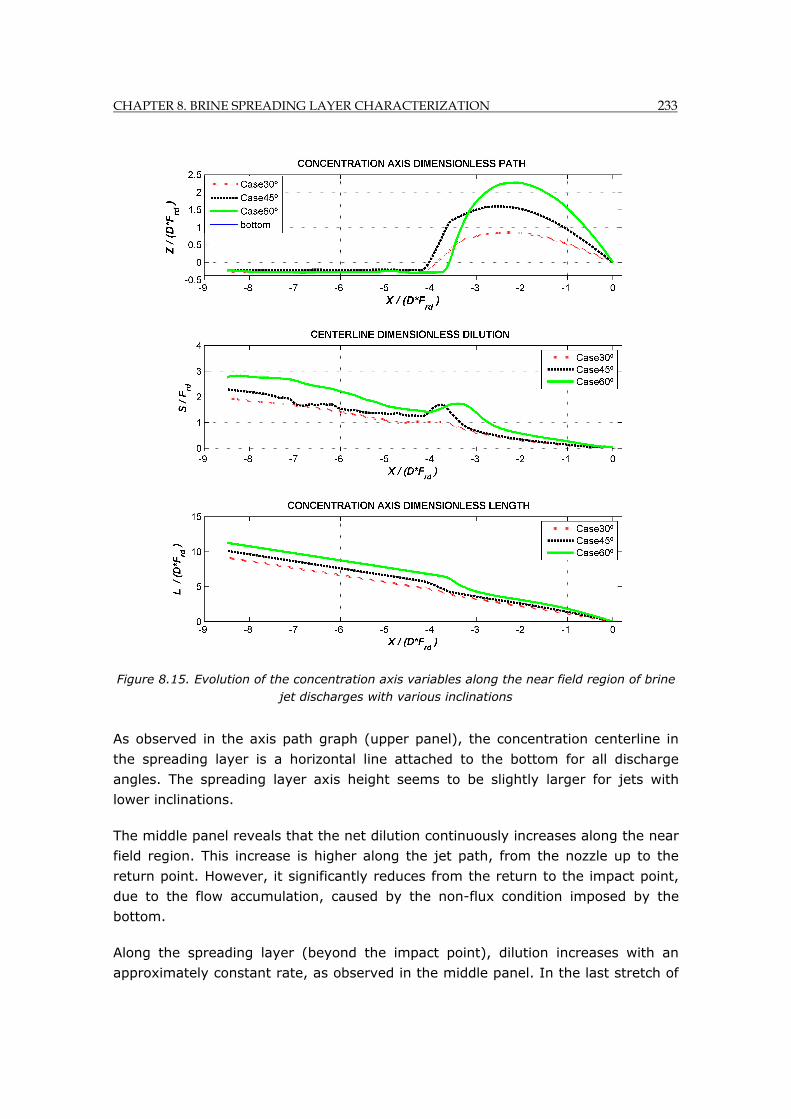
CHAPTER 8. BRINE SPREADING LAYER CHARACTERIZATION 233
Figure 8.15. Evolution of the concentration axis variables along the near field region of brine jet discharges with various inclinations
As observed in the axis path graph (upper panel), the concentration centerline in
the spreading layer is a horizontal line attached to the bottom for all discharge
angles. The spreading layer axis height seems to be slightly larger for jets with
lower inclinations.
The middle panel reveals that the net dilution continuously increases along the near
field region. This increase is higher along the jet path, from the nozzle up to the
return point. However, it significantly reduces from the return to the impact point,
due to the flow accumulation, caused by the non-flux condition imposed by the
bottom.
Along the spreading layer (beyond the impact point), dilution increases with an
approximately constant rate, as observed in the middle panel. In the last stretch of
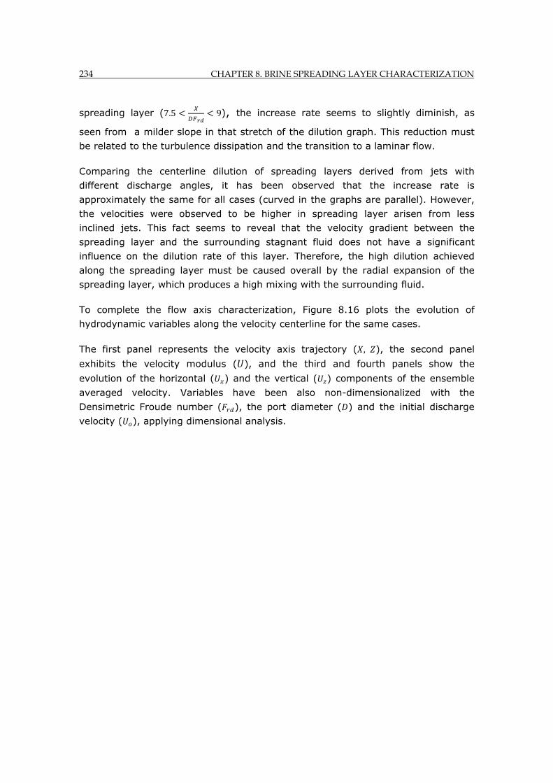
234 CHAPTER 8. BRINE SPREADING LAYER CHARACTERIZATION
spreading layer (7.5 9), the increase rate seems to slightly diminish, as
seen from a milder slope in that stretch of the dilution graph. This reduction must
be related to the turbulence dissipation and the transition to a laminar flow.
Comparing the centerline dilution of spreading layers derived from jets with
different discharge angles, it has been observed that the increase rate is
approximately the same for all cases (curved in the graphs are parallel). However,
the velocities were observed to be higher in spreading layer arisen from less
inclined jets. This fact seems to reveal that the velocity gradient between the
spreading layer and the surrounding stagnant fluid does not have a significant
influence on the dilution rate of this layer. Therefore, the high dilution achieved
along the spreading layer must be caused overall by the radial expansion of the
spreading layer, which produces a high mixing with the surrounding fluid.
To complete the flow axis characterization, Figure 8.16 plots the evolution of
hydrodynamic variables along the velocity centerline for the same cases.
The first panel represents the velocity axis trajectory ( , ), the second panel
exhibits the velocity modulus ( ), and the third and fourth panels show the
evolution of the horizontal ( ) and the vertical ( ) components of the ensemble
averaged velocity. Variables have been also non-dimensionalized with the
Densimetric Froude number ( ), the port diameter ( ) and the initial discharge
velocity ( ), applying dimensional analysis.
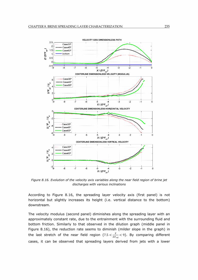
CHAPTER 8. BRINE SPREADING LAYER CHARACTERIZATION 235
Figure 8.16. Evolution of the velocity axis variables along the near field region of brine jet discharges with various inclinations
According to Figure 8.16, the spreading layer velocity axis (first panel) is not
horizontal but slightly increases its height (i.e. vertical distance to the bottom)
downstream.
The velocity modulus (second panel) diminishes along the spreading layer with an
approximately constant rate, due to the entrainment with the surrounding fluid and
bottom friction. Similarly to that observed in the dilution graph (middle panel in
Figure 8.16), the reduction rate seems to diminish (milder slope in the graph) in
the last stretch of the near field region (7.5 9). By comparing different
cases, it can be observed that spreading layers derived from jets with a lower
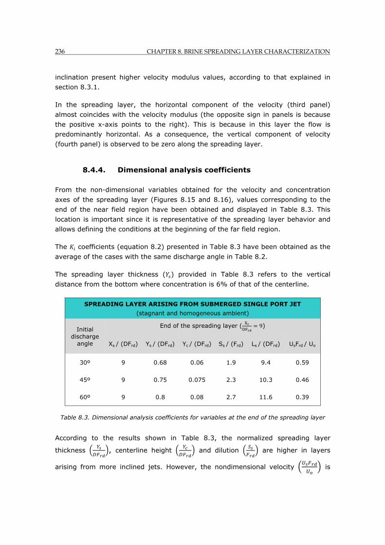
236 CHAPTER 8. BRINE SPREADING LAYER CHARACTERIZATION
inclination present higher velocity modulus values, according to that explained in
section 8.3.1.
In the spreading layer, the horizontal component of the velocity (third panel)
almost coincides with the velocity modulus (the opposite sign in panels is because
the positive x-axis points to the right). This is because in this layer the flow is
predominantly horizontal. As a consequence, the vertical component of velocity
(fourth panel) is observed to be zero along the spreading layer.
8.4.4. Dimensional analysis coefficients
From the non-dimensional variables obtained for the velocity and concentration
axes of the spreading layer (Figures 8.15 and 8.16), values corresponding to the
end of the near field region have been obtained and displayed in Table 8.3. This
location is important since it is representative of the spreading layer behavior and
allows defining the conditions at the beginning of the far field region.
The coefficients (equation 8.2) presented in Table 8.3 have been obtained as the
average of the cases with the same discharge angle in Table 8.2.
The spreading layer thickness ( ) provided in Table 8.3 refers to the vertical
distance from the bottom where concentration is 6% of that of the centerline.
SPREADING LAYER ARISING FROM SUBMERGED SINGLE PORT JET
(stagnant and homogeneous ambient)
Initial discharge
angle
End of the spreading layer ( X
DF9)
Xs / (DFrd) Ys / (DFrd) Yc / (DFrd) Ss / (Frd) Ls / (DFrd) UsFrd / Uo
30º 9 0.68 0.06 1.9 9.4 0.59
45º 9 0.75 0.075 2.3 10.3 0.46
60º 9 0.8 0.08 2.7 11.6 0.39
Table 8.3. Dimensional analysis coefficients for variables at the end of the spreading layer
According to the results shown in Table 8.3, the normalized spreading layer
thickness , centerline height and dilution are higher in layers
arising from more inclined jets. However, the nondimensional velocity is
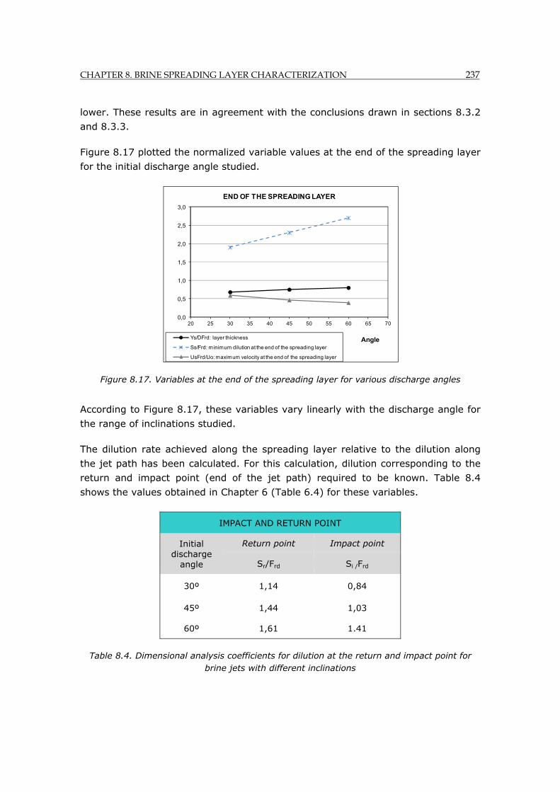
CHAPTER 8. BRINE SPREADING LAYER CHARACTERIZATION 237
lower. These results are in agreement with the conclusions drawn in sections 8.3.2
and 8.3.3.
Figure 8.17 plotted the normalized variable values at the end of the spreading layer
for the initial discharge angle studied.
Figure 8.17. Variables at the end of the spreading layer for various discharge angles
According to Figure 8.17, these variables vary linearly with the discharge angle for
the range of inclinations studied.
The dilution rate achieved along the spreading layer relative to the dilution along
the jet path has been calculated. For this calculation, dilution corresponding to the
return and impact point (end of the jet path) required to be known. Table 8.4
shows the values obtained in Chapter 6 (Table 6.4) for these variables.
IMPACT AND RETURN POINT
Initial discharge
angle
Return point Impact point
Sr/Frd Si /Frd
30º 1,14 0,84
45º 1,44 1,03
60º 1,61 1.41
Table 8.4. Dimensional analysis coefficients for dilution at the return and impact point for brine jets with different inclinations
0,0
0,5
1,0
1,5
2,0
2,5
3,0
20 25 30 35 40 45 50 55 60 65 70
Angle
END OF THE SPREADING LAYER
Ys/DFrd: layer thickness
Ss/Frd: minimum dilution at the end of the spreading layer
UsFrd/Uo: maximum velocity at the end of the spreading layer
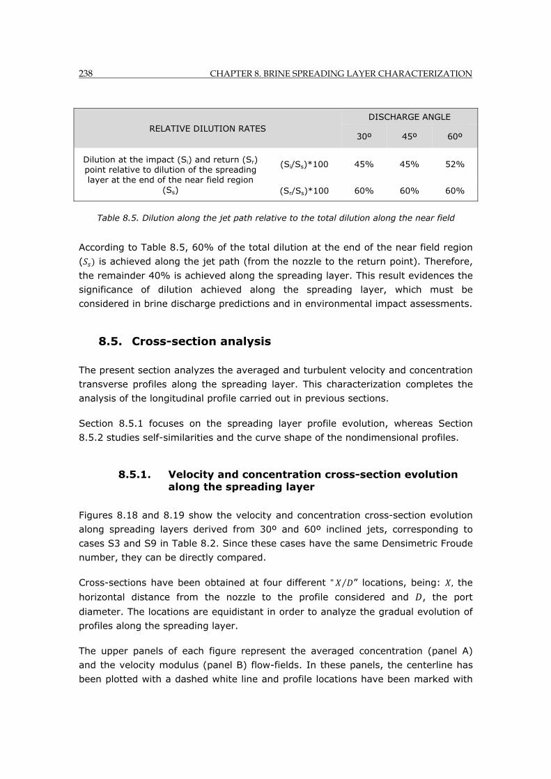
238 CHAPTER 8. BRINE SPREADING LAYER CHARACTERIZATION
Table 8.5. Dilution along the jet path relative to the total dilution along the near field
According to Table 8.5, 60% of the total dilution at the end of the near field region
( is achieved along the jet path (from the nozzle to the return point). Therefore,
the remainder 40% is achieved along the spreading layer. This result evidences the
significance of dilution achieved along the spreading layer, which must be
considered in brine discharge predictions and in environmental impact assessments.
8.5. Cross-section analysis
The present section analyzes the averaged and turbulent velocity and concentration
transverse profiles along the spreading layer. This characterization completes the
analysis of the longitudinal profile carried out in previous sections.
Section 8.5.1 focuses on the spreading layer profile evolution, whereas Section
8.5.2 studies self-similarities and the curve shape of the nondimensional profiles.
8.5.1. Velocity and concentration cross-section evolution along the spreading layer
Figures 8.18 and 8.19 show the velocity and concentration cross-section evolution
along spreading layers derived from 30º and 60º inclined jets, corresponding to
cases S3 and S9 in Table 8.2. Since these cases have the same Densimetric Froude
number, they can be directly compared.
Cross-sections have been obtained at four different " ⁄ ” locations, being: , the
horizontal distance from the nozzle to the profile considered and , the port
diameter. The locations are equidistant in order to analyze the gradual evolution of
profiles along the spreading layer.
The upper panels of each figure represent the averaged concentration (panel A)
and the velocity modulus (panel B) flow-fields. In these panels, the centerline has
been plotted with a dashed white line and profile locations have been marked with
RELATIVE DILUTION RATES DISCHARGE ANGLE
30º 45º 60º
Dilution at the impact (Si) and return (Sr) point relative to dilution of the spreading layer at the end of the near field region
(Ss)
(Si/Ss)*100 45% 45% 52%
(Sr/Ss)*100 60% 60% 60%
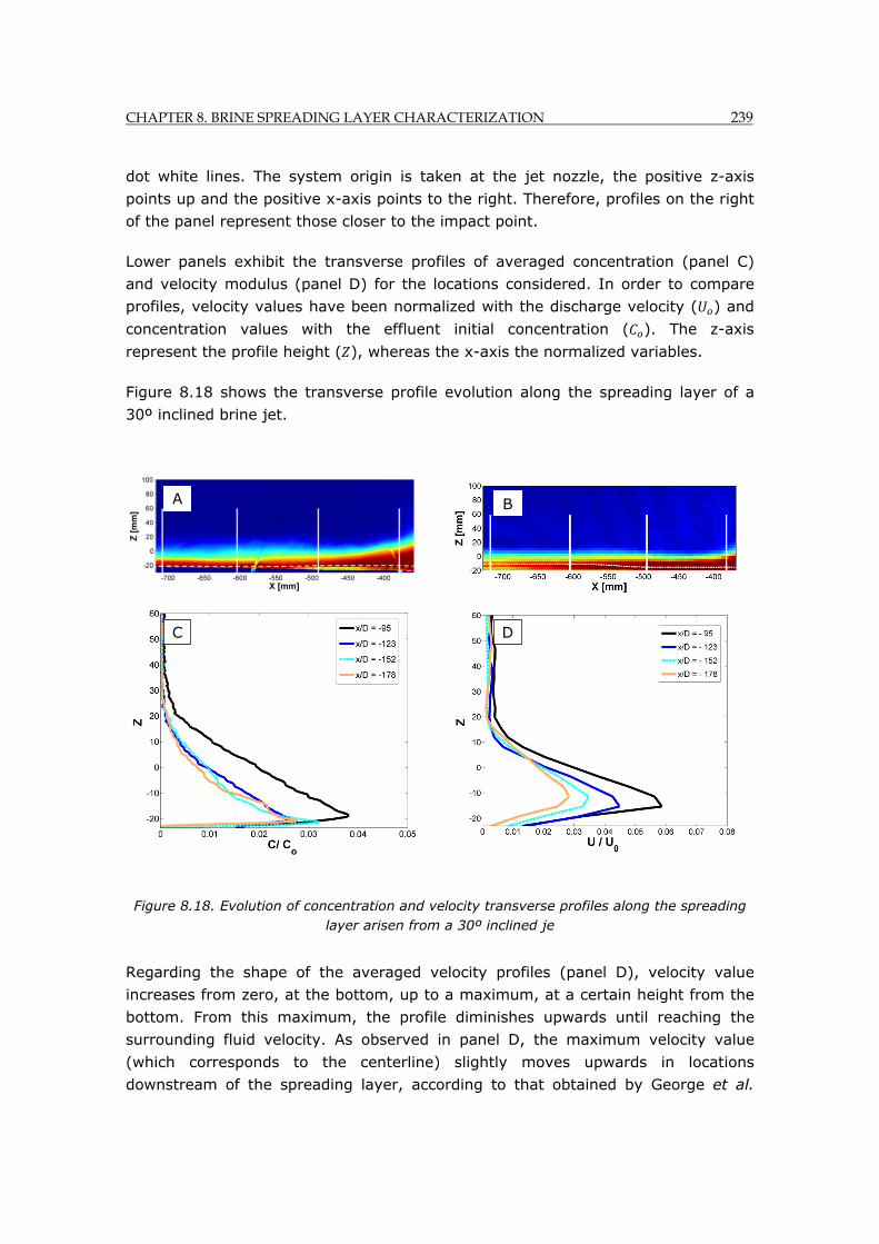
CHAPTER 8. BRINE SPREADING LAYER CHARACTERIZATION 239
dot white lines. The system origin is taken at the jet nozzle, the positive z-axis
points up and the positive x-axis points to the right. Therefore, profiles on the right
of the panel represent those closer to the impact point.
Lower panels exhibit the transverse profiles of averaged concentration (panel C)
and velocity modulus (panel D) for the locations considered. In order to compare
profiles, velocity values have been normalized with the discharge velocity ( ) and
concentration values with the effluent initial concentration ( ). The z-axis
represent the profile height ( ), whereas the x-axis the normalized variables.
Figure 8.18 shows the transverse profile evolution along the spreading layer of a
30º inclined brine jet.
Figure 8.18. Evolution of concentration and velocity transverse profiles along the spreading layer arisen from a 30º inclined je
Regarding the shape of the averaged velocity profiles (panel D), velocity value
increases from zero, at the bottom, up to a maximum, at a certain height from the
bottom. From this maximum, the profile diminishes upwards until reaching the
surrounding fluid velocity. As observed in panel D, the maximum velocity value
(which corresponds to the centerline) slightly moves upwards in locations
downstream of the spreading layer, according to that obtained by George et al.
A B
C D
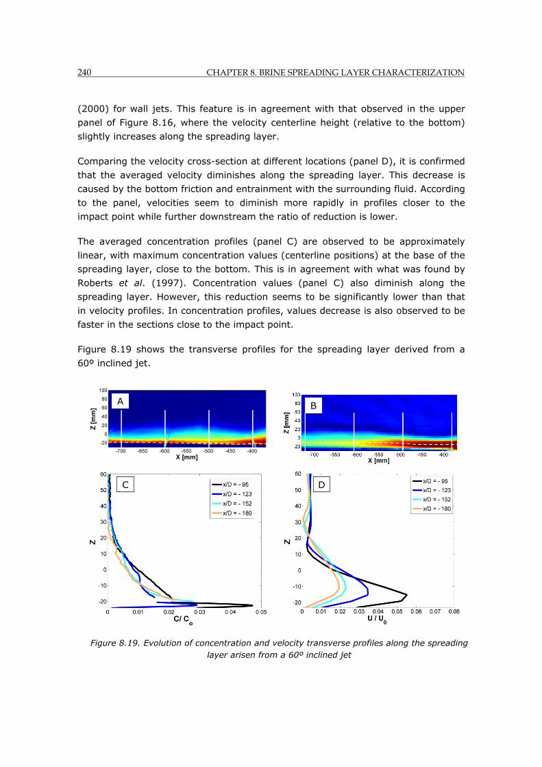
240 CHAPTER 8. BRINE SPREADING LAYER CHARACTERIZATION
(2000) for wall jets. This feature is in agreement with that observed in the upper
panel of Figure 8.16, where the velocity centerline height (relative to the bottom)
slightly increases along the spreading layer.
Comparing the velocity cross-section at different locations (panel D), it is confirmed
that the averaged velocity diminishes along the spreading layer. This decrease is
caused by the bottom friction and entrainment with the surrounding fluid. According
to the panel, velocities seem to diminish more rapidly in profiles closer to the
impact point while further downstream the ratio of reduction is lower.
The averaged concentration profiles (panel C) are observed to be approximately
linear, with maximum concentration values (centerline positions) at the base of the
spreading layer, close to the bottom. This is in agreement with what was found by
Roberts et al. (1997). Concentration values (panel C) also diminish along the
spreading layer. However, this reduction seems to be significantly lower than that
in velocity profiles. In concentration profiles, values decrease is also observed to be
faster in the sections close to the impact point.
Figure 8.19 shows the transverse profiles for the spreading layer derived from a
60º inclined jet.
0
D
A B
C
Figure 8.19. Evolution of concentration and velocity transverse profiles along the spreading layer arisen from a 60º inclined jet
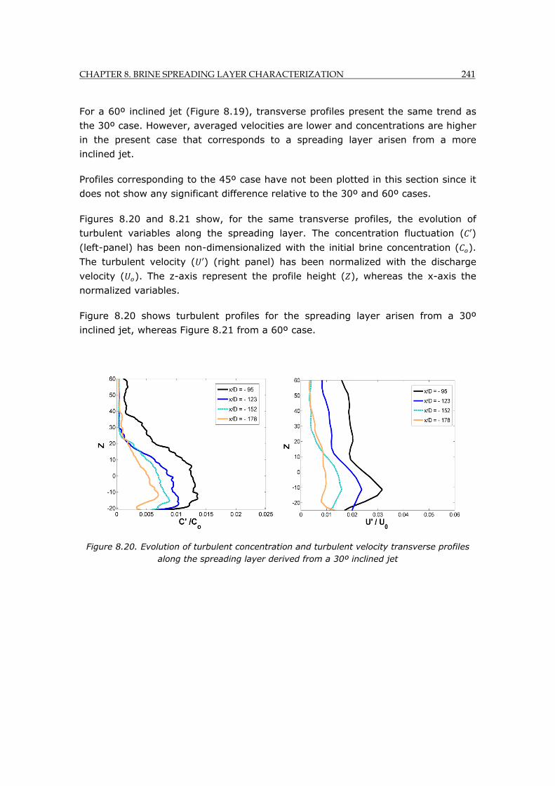
CHAPTER 8. BRINE SPREADING LAYER CHARACTERIZATION 241
For a 60º inclined jet (Figure 8.19), transverse profiles present the same trend as
the 30º case. However, averaged velocities are lower and concentrations are higher
in the present case that corresponds to a spreading layer arisen from a more
inclined jet.
Profiles corresponding to the 45º case have not been plotted in this section since it
does not show any significant difference relative to the 30º and 60º cases.
Figures 8.20 and 8.21 show, for the same transverse profiles, the evolution of
turbulent variables along the spreading layer. The concentration fluctuation ( )
(left-panel) has been non-dimensionalized with the initial brine concentration ( ).
The turbulent velocity ( ) (right panel) has been normalized with the discharge
velocity ( ). The z-axis represent the profile height ( ), whereas the x-axis the
normalized variables.
Figure 8.20 shows turbulent profiles for the spreading layer arisen from a 30º
inclined jet, whereas Figure 8.21 from a 60º case.
Figure 8.20. Evolution of turbulent concentration and turbulent velocity transverse profiles along the spreading layer derived from a 30º inclined jet
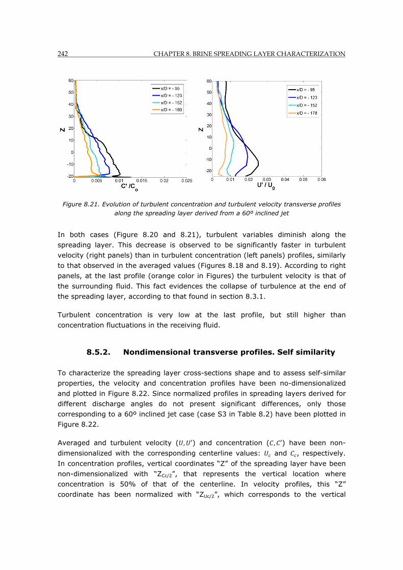
242 CHAPTER 8. BRINE SPREADING LAYER CHARACTERIZATION
Figure 8.21. Evolution of turbulent concentration and turbulent velocity transverse profiles along the spreading layer derived from a 60º inclined jet
In both cases (Figure 8.20 and 8.21), turbulent variables diminish along the
spreading layer. This decrease is observed to be significantly faster in turbulent
velocity (right panels) than in turbulent concentration (left panels) profiles, similarly
to that observed in the averaged values (Figures 8.18 and 8.19). According to right
panels, at the last profile (orange color in Figures) the turbulent velocity is that of
the surrounding fluid. This fact evidences the collapse of turbulence at the end of
the spreading layer, according to that found in section 8.3.1.
Turbulent concentration is very low at the last profile, but still higher than
concentration fluctuations in the receiving fluid.
8.5.2. Nondimensional transverse profiles. Self similarity
To characterize the spreading layer cross-sections shape and to assess self-similar
properties, the velocity and concentration profiles have been no-dimensionalized
and plotted in Figure 8.22. Since normalized profiles in spreading layers derived for
different discharge angles do not present significant differences, only those
corresponding to a 60º inclined jet case (case S3 in Table 8.2) have been plotted in
Figure 8.22.
Averaged and turbulent velocity ( , ) and concentration ( , ) have been non-
dimensionalized with the corresponding centerline values: and , respectively.
In concentration profiles, vertical coordinates “Z” of the spreading layer have been
non-dimensionalized with “ZCc/2”, that represents the vertical location where
concentration is 50% of that of the centerline. In velocity profiles, this “Z”
coordinate has been normalized with “ZUc/2”, which corresponds to the vertical
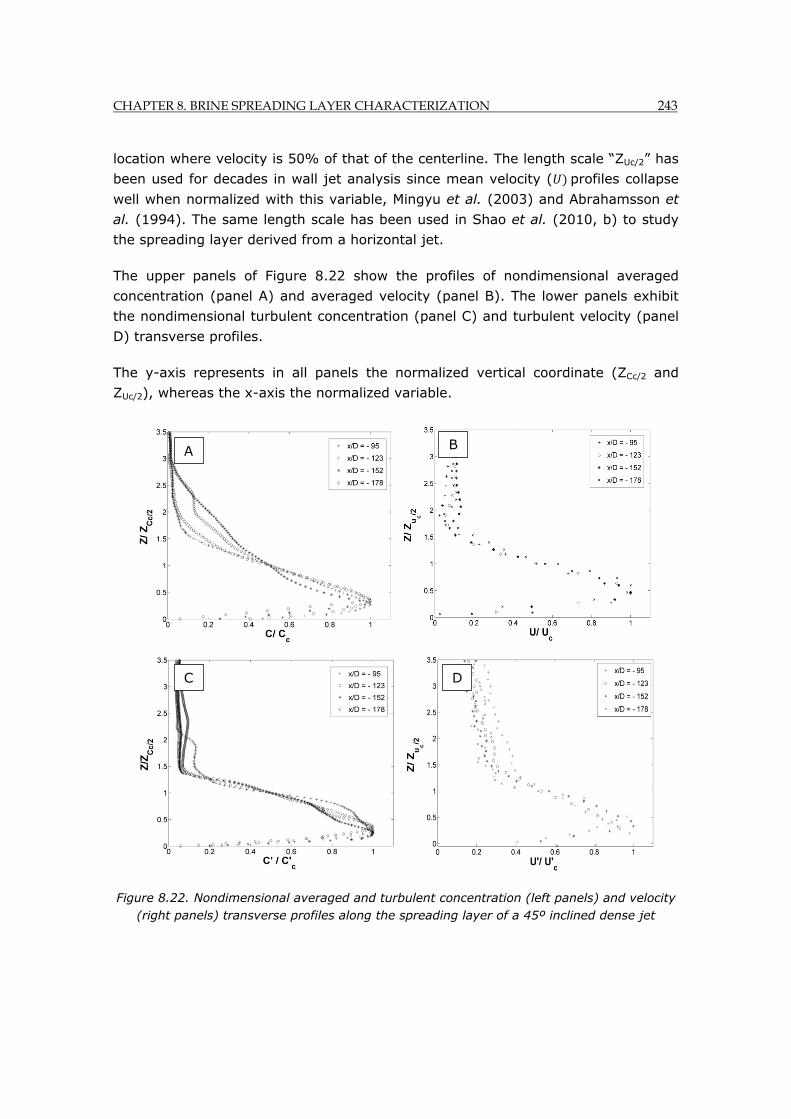
CHAPTER 8. BRINE SPREADING LAYER CHARACTERIZATION 243
location where velocity is 50% of that of the centerline. The length scale “ZUc/2” has
been used for decades in wall jet analysis since mean velocity ( profiles collapse
well when normalized with this variable, Mingyu et al. (2003) and Abrahamsson et
al. (1994). The same length scale has been used in Shao et al. (2010, b) to study
the spreading layer derived from a horizontal jet.
The upper panels of Figure 8.22 show the profiles of nondimensional averaged
concentration (panel A) and averaged velocity (panel B). The lower panels exhibit
the nondimensional turbulent concentration (panel C) and turbulent velocity (panel
D) transverse profiles.
The y-axis represents in all panels the normalized vertical coordinate (ZCc/2 and
ZUc/2), whereas the x-axis the normalized variable.
Figure 8.22. Nondimensional averaged and turbulent concentration (left panels) and velocity (right panels) transverse profiles along the spreading layer of a 45º inclined dense jet
A B
C D
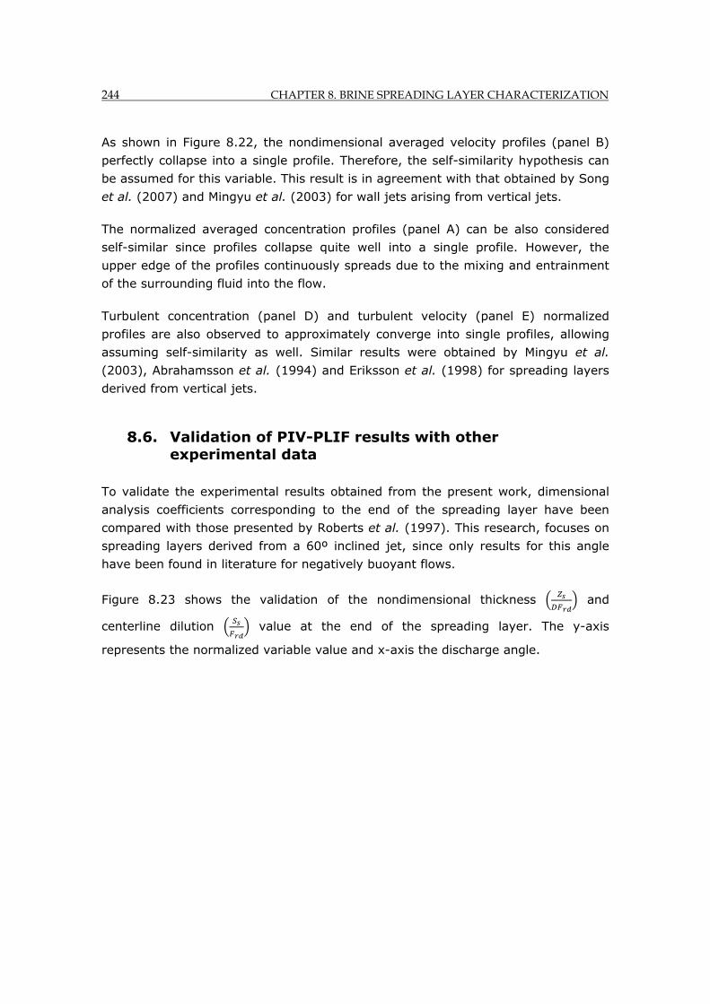
244 CHAPTER 8. BRINE SPREADING LAYER CHARACTERIZATION
As shown in Figure 8.22, the nondimensional averaged velocity profiles (panel B)
perfectly collapse into a single profile. Therefore, the self-similarity hypothesis can
be assumed for this variable. This result is in agreement with that obtained by Song
et al. (2007) and Mingyu et al. (2003) for wall jets arising from vertical jets.
The normalized averaged concentration profiles (panel A) can be also considered
self-similar since profiles collapse quite well into a single profile. However, the
upper edge of the profiles continuously spreads due to the mixing and entrainment
of the surrounding fluid into the flow.
Turbulent concentration (panel D) and turbulent velocity (panel E) normalized
profiles are also observed to approximately converge into single profiles, allowing
assuming self-similarity as well. Similar results were obtained by Mingyu et al.
(2003), Abrahamsson et al. (1994) and Eriksson et al. (1998) for spreading layers
derived from vertical jets.
8.6. Validation of PIV-PLIF results with other experimental data
To validate the experimental results obtained from the present work, dimensional
analysis coefficients corresponding to the end of the spreading layer have been
compared with those presented by Roberts et al. (1997). This research, focuses on
spreading layers derived from a 60º inclined jet, since only results for this angle
have been found in literature for negatively buoyant flows.
Figure 8.23 shows the validation of the nondimensional thickness and
centerline dilution value at the end of the spreading layer. The y-axis
represents the normalized variable value and x-axis the discharge angle.
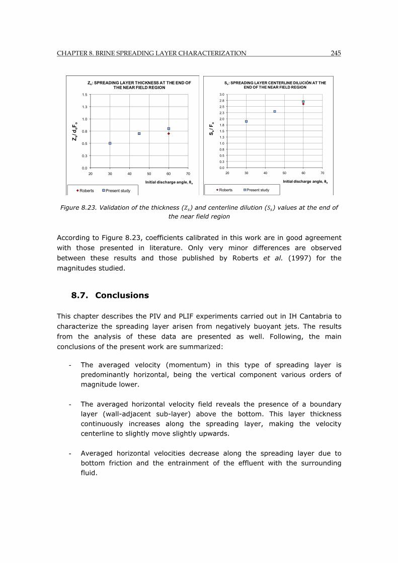
CHAPTER 8. BRINE SPREADING LAYER CHARACTERIZATION 245
Figure 8.23. Validation of the thickness ( ) and centerline dilution ( ) values at the end of the near field region
According to Figure 8.23, coefficients calibrated in this work are in good agreement
with those presented in literature. Only very minor differences are observed
between these results and those published by Roberts et al. (1997) for the
magnitudes studied.
8.7. Conclusions
This chapter describes the PIV and PLIF experiments carried out in IH Cantabria to
characterize the spreading layer arisen from negatively buoyant jets. The results
from the analysis of these data are presented as well. Following, the main
conclusions of the present work are summarized:
- The averaged velocity (momentum) in this type of spreading layer is predominantly horizontal, being the vertical component various orders of magnitude lower.
- The averaged horizontal velocity field reveals the presence of a boundary layer (wall-adjacent sub-layer) above the bottom. This layer thickness continuously increases along the spreading layer, making the velocity centerline to slightly move slightly upwards.
- Averaged horizontal velocities decrease along the spreading layer due to bottom friction and the entrainment of the effluent with the surrounding fluid.
0.0
0.3
0.5
0.8
1.0
1.3
1.5
20 30 40 50 60 70
Zs/ d
oF
o
Initial discharge angle, θo
Zs: SPREADING LAYER THICKNESS AT THE END OF THE NEAR FIELD REGION
Roberts Present study
0.0
0.3
0.5
0.8
1.0
1.3
1.5
1.8
2.0
2.3
2.5
2.8
3.0
20 30 40 50 60 70
Ss
/ F
o
Initial discharge angle, θo
Ss: SPREADING LAYER CENTERLINE DILUCIÓN AT THE END OF THE NEAR FIELD REGION
Roberts Present study

246 CHAPTER 8. BRINE SPREADING LAYER CHARACTERIZATION
- For jets with the same Densimetric Froude number, velocity modulus along the spreading layer is observed to be higher in jets with lower discharge angles. This is in agreement with larger horizontal velocities at the impact point.
- The horizontal and vertical components of the turbulent velocity are significant in the beginning of the spreading layer, having values of the same order of magnitude as the averaged horizontal velocity. Velocity fluctuations continuously decrease downstream, being almost zero at the end of the spreading layer. This feature reveals the collapse of turbulence. Similarly to averaged velocities, turbulent values are lower in spreading layers derived from jets with a higher inclination.
- For jets with the same Densimetric Froude number, the dilution achieved at the end of the spreading layer is larger for spreading layers arisen from more inclined jets.
- Dilution increases linearly along the spreading layer, with a similar rate in all cases, which seems to be independently on the discharge angle.
- The highest turbulent concentrations relative to average concentrations are located at the interface between the spreading layer and the surrounding fluid. In this zone, Kelvin-Helmholtz vortices appear, rotating clockwise and causing the mixing between fluids. These vortices are dissipated along the spreading layer, according to the collapse of turbulence.
- The evolution of variables along the velocity and concentration centerlines presented in this work allows comparing the behaviour and the main features of spreading layers arisen from jets with different discharge angles.
- Dimensional analysis coefficients to characterize the spreading layer have been calibrated with the PIV and PLIF experimental data obtained for 30º, 45º and 60º cases. Results reveal that, for jets with larger inclinations, the layer thickness and the centerline dilution are higher, whereas the maximum velocity is lower. These variables vary linearly with the discharge angle for the range of cases studied.
- The analysis of velocity and concentration transverse profiles along the spreading layer confirms the decrease of these variables downstream. Velocities are observed to diminish more rapidly than concentrations.
- In averaged velocity transverse profiles, velocities are zero at the bottom as a consequence of the presence of this boundary. From this value on, velocity

CHAPTER 8. BRINE SPREADING LAYER CHARACTERIZATION 247
increases up to a maximum, located at a certain distance from the bottom. From this maximum (corresponding to the centerline), values decrease upwards until reaching the surrounding fluid velocity.
- In averaged concentration profiles, the maximum value (corresponding to the centerline) is located at the bottom. This is due to the non-flux condition imposed across this boundary, making the flow to accumulate at the bottom. From this maximum, concentration decreases upwards with an approximately linear rate up to reach the surrounding fluid concentration.
- The nondimensional transverse profiles reveal that self-similarities properties can be assumed for the averaged and turbulent velocity and concentration profiles along the spreading layer.
The present research is, to our knowledge, the first one including a detailed
description of the behavior of spreading layers derived from negatively buoyant
inclined jets. The study covers discharge angles in the range 30° 60° and
carries out an in-depth analysis of the averaged and turbulent velocity and
concentration variables. The calibrated dimensional analysis formulas provide a
quantitative assessment of the spreading layer features. This allows defining the
flow conditions at the beginning of the far field region.

248 CHAPTER 8. BRINE SPREADING LAYER CHARACTERIZATION

CHAPTER 9. NEW “BRIHNE” NUMERICAL TOOLS 249
Chapter 9. NEW “BRIHNE” NUMERICAL TOOLS TO SIMULATE BRINE DISCHARGES
Chapter 9 NEW “BRIHNE” NUMERICAL TOOLS TO SIMULATE BRINE DISCHARGES
Summary
Numerical modeling is a fundamental tool in environmental impact assessment of
desalination plants since it predicts the brine discharge behavior and allows
assessing the performance of water quality standards established to protect the
marine receiving waters.
Faced with the commercial model limitations to simulate brine discharges and their
poor agreement with experimental data (Chapters 3 and 4), alternative “BrIHne”
simulation tools have been developed for a more accurate prediction of brine
behavior. They focus on the simulation of discharges through submerged jets,
covering different modeling scopes (near field region, far field region or both) and
design parameters.
To make “BrIHne” tools useful in real desalination plant projects, they are available
to users through a website.
Three of these models are described in detail in the present chapter: brIHne-Jet,
brIHne-Jet-Spreading and brIHne-Jet-Plume. These models, which respond to
different mathematical approaches, have been re-calibrated with the PIV and PLIF
experimental data presented in this thesis. Useful information, such as Technical
Specifications or recommended input data, has been developed for each model.
250 CHAPTER 9. NEW “BRIHNE” NUMERICAL TOOLS
9.1. Introduction
Water quality modeling is a mathematical representation of the physical
mechanisms determining the evolution of pollutant concentrations discharged into a
receiving body. It involves the prediction of water pollution using mathematical
simulation techniques and considering the effluent properties, the discharge
configuration and the ambient conditions. Water quality modeling applied to brine
discharges solves the hydrodynamics and transport equations adapted to a
negatively buoyant effluent.
9.1.1. Governing equations
Simplifying assumptions within modeling
Simplifying assumptions, which are generally taken in the modeling of brine
discharges are, Doneker et al. (2001):
1.) Incompressible flow (pressure does not affect density of the fluid).
2.) Reynolds decomposition: , the instantaneous value of a
magnitude is the sum of a time-averaged component and a random (instant,
turbulent) component.
3) Boussinesq approximation: density differences between effluent discharges and
the water receiving environment are small and are important only in terms of the
buoyancy force.
4) Turbulence closure model based on Boussinesq turbulent viscosity theory,
. Turbulent terms are proportional to the average value of the
magnitude, with an experimental proportionality coefficient (eddy viscosity). In
recent years, more rigorous and sophisticated closure models, such as the k-ε
model, are being applied.
5) Molecular diffusion is negligible compared to turbulent diffusion in the effluent.
Chemical processes are not considered.
6) There are no fluid sources or drain.
Once the simplifying assumptions have been applied, the partial differential
equations to be solved in brine discharge modeling are:
CHAPTER 9. NEW “BRIHNE” NUMERICAL TOOLS 251
Equation of Continuity (Mass Conservation)
It is a statement of mass conservation. For a control volume having a single inlet
and a single outlet, the principle of mass conservation states that, for steady-state
flow, the mass flow rate into the volume must equal the mass flow rate out of it. It
relates velocity and density of the fluid.
0 9.1
In Cartesian coordinates: 0 (9.2)
Equation of momentum conservation
The momentum equation is a statement of Newton's Second Law and relates the
sum of the forces acting on a fluid element (incompressible) to its acceleration or
momentum change rate:∑ . Total force is the sum of surface forces (viscous
stresses) acting by direct contact, and volume forces (inertial) acting without
contact.
1 9.3
Cartesian coordinates:
X Axis: (9.4)
Y Axis: (9.5)
Z Axis: (9.6)
Transport equation (Conservation of Solute mass)
For a control volume, changes in concentration (salinity) are due to the advective
transport of fluid containing the substance, solute mass flow by diffusion, and
destruction or incorporation of the substance in the fluid. In Cartesian coordinates:
9.7
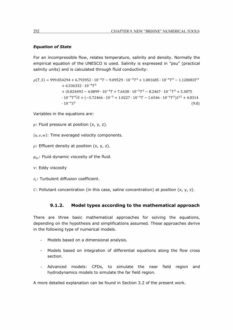
252 CHAPTER 9. NEW “BRIHNE” NUMERICAL TOOLS
Equation of State
For an incompressible flow, relates temperature, salinity and density. Normally the
empirical equation of the UNESCO is used. Salinity is expressed in "psu” (practical
salinity units) and is calculated through fluid conductivity:
, 999.854294 6.793952 · 10 9.09529 · 10 1.001685 · 10 1.120083
6.536332 · 10
0.824493 4.0899 · 10 7.6438 · 10 8.2467 · 10 5.3875
· 10 5.72466 · 10 1.0227 · 10 1.6546 · 10 4.8314
· 10 9.8
Variables in the equations are:
: Fluid pressure at position (x, y, z).
, , : Time averaged velocity components.
: Effluent density at position (x, y, z).
: Fluid dynamic viscosity of the fluid.
: Eddy viscosity
: Turbulent diffusion coefficient.
: Pollutant concentration (in this case, saline concentration) at position (x, y, z).
9.1.2. Model types according to the mathematical approach
There are three basic mathematical approaches for solving the equations,
depending on the hypothesis and simplifications assumed. These approaches derive
in the following type of numerical models.
- Models based on a dimensional analysis.
- Models based on integration of differential equations along the flow cross section.
- Advanced models: CFDs, to simulate the near field region and hydrodynamics models to simulate the far field region.
A more detailed explanation can be found in Section 3.2 of the present work.
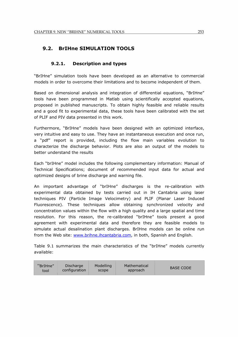
CHAPTER 9. NEW “BRIHNE” NUMERICAL TOOLS 253
9.2. BrIHne SIMULATION TOOLS
9.2.1. Description and types
“BrIHne” simulation tools have been developed as an alternative to commercial
models in order to overcome their limitations and to become independent of them.
Based on dimensional analysis and integration of differential equations, “BrIHne”
tools have been programmed in Matlab using scientifically accepted equations,
proposed in published manuscripts. To obtain highly feasible and reliable results
and a good fit to experimental data, these tools have been calibrated with the set
of PLIF and PIV data presented in this work.
Furthermore, “BrIHne” models have been designed with an optimized interface,
very intuitive and easy to use. They have an instantaneous execution and once run,
a “pdf” report is provided, including the flow main variables evolution to
characterize the discharge behavior. Plots are also an output of the models to
better understand the results
Each “brIHne” model includes the following complementary information: Manual of
Technical Specifications; document of recommended input data for actual and
optimized designs of brine discharge and warning file.
An important advantage of “brIHne” discharges is the re-calibration with
experimental data obtained by tests carried out in IH Cantabria using laser
techniques PIV (Particle Image Velocimetry) and PLIF (Planar Laser Induced
Fluorescence). These techniques allow obtaining synchronized velocity and
concentration values within the flow with a high quality and a large spatial and time
resolution. For this reason, the re-calibrated “brIHne” tools present a good
agreement with experimental data and therefore they are feasible models to
simulate actual desalination plant discharges. BrIHne models can be online run
from the Web site: www.brihne.ihcantabria.com, in both, Spanish and English.
Table 9.1 summarizes the main characteristics of the “brIHne” models currently
available:
“BrIHne” tool
Discharge configuration
Modelling scope
Mathematical approach
BASE CODE
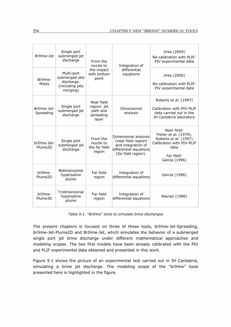
254 CHAPTER 9. NEW “BRIHNE” NUMERICAL TOOLS
BrIHne-Jet Single port
submerged jet discharge From the
nozzle to the impact
with bottom point
Integration of differential equations
Jirka (2004)
Re-calibration with PLIF-PIV experimental data
BrIHne-MJets
Multi-port submerged jets
discharge. (including jets
merging)
Jirka (2006)
Re-calibration with PLIF-PIV experimental data
BrIHne-Jet-Spreading
Single port submerged jet
discharge
Near field region: jet path and spreading
layer
Dimensional analysis
Roberts et al. (1997)
Calibration with PIV-PLIF data carried out in the IH Cantabria laboratory
brIHne-Jet-Plume2D
Single port submerged jet
discharge
From the nozzle to
the far field region
Dimensional analysis (near field region) and integration of
differential equations (far field region).
Near field: Fisher et al. (1979), Roberts et al. (1997)
Calibration with PIV-PLIF data
Far field:
García (1996)
brIHne-Plume2D
Bidimensional hypersaline
plume
Far field region
Integration of differential equations
García (1996)
brIHne-Plume3D
Tridimensional hypersaline
plume
Far field region
Integration of differential equations
Alavian (1986)
Table 9.1. “BrIHne” tools to simulate brine discharges
The present chapters is focused on three of these tools, brIHne-Jet-Spreading,
brIHne-Jet-Plume2D and BrIHne-Jet, which simulates the behavior of a submerged
single port jet brine discharge under different mathematical approaches and
modeling scopes. The two first models have been already calibrated with the PIV
and PLIF experimental data obtained and presented in this work.
Figure 9.1 shows the picture of an experimental test carried out in IH Cantabria,
simulating a brine jet discharge. The modeling scope of the “brIHne” tools
presented here is highlighted in the figure.
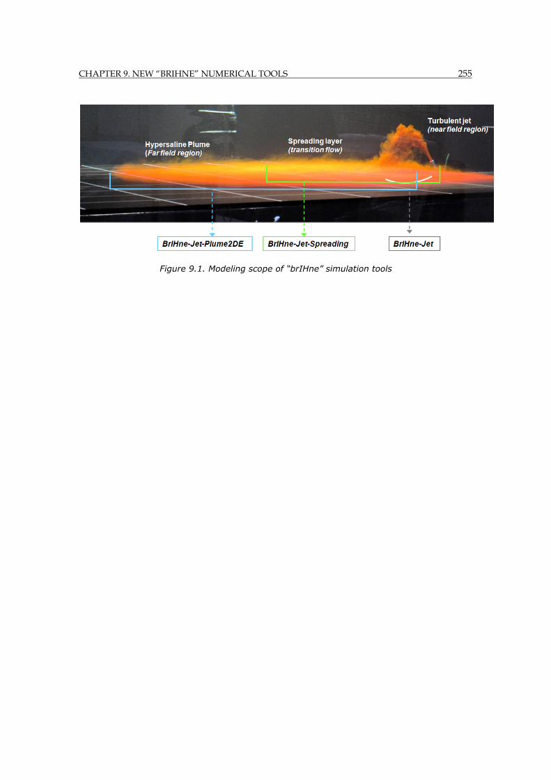
CHAPTER 9. NEW “BRIHNE” NUMERICAL TOOLS 255
Figure 9.1. Modeling scope of “brIHne” simulation tools
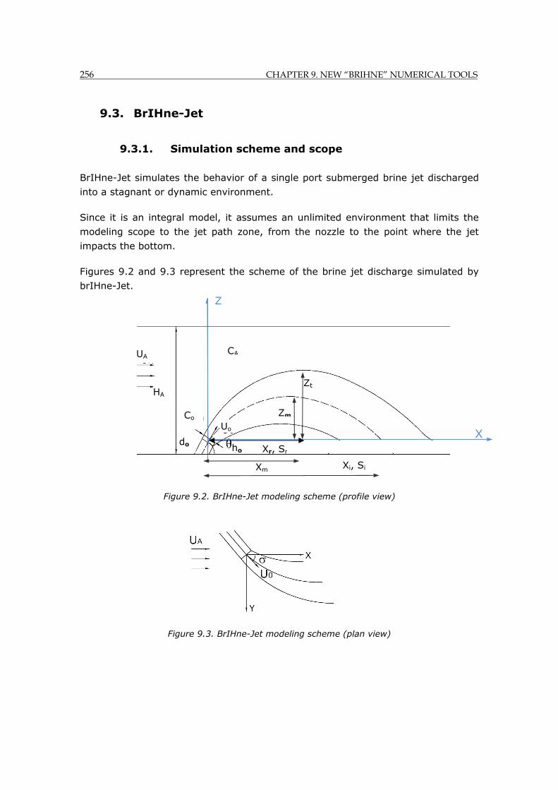
256 CHAPTER 9. NEW “BRIHNE” NUMERICAL TOOLS
9.3. BrIHne-Jet
9.3.1. Simulation scheme and scope
BrIHne-Jet simulates the behavior of a single port submerged brine jet discharged
into a stagnant or dynamic environment.
Since it is an integral model, it assumes an unlimited environment that limits the
modeling scope to the jet path zone, from the nozzle to the point where the jet
impacts the bottom.
Figures 9.2 and 9.3 represent the scheme of the brine jet discharge simulated by
brIHne-Jet.
Figure 10.2. BrIHne_JET modeling scheme (profile view).
Figure 9.2. BrIHne-Jet modeling scheme (profile view)
Figure 9.3. BrIHne-Jet modeling scheme (plan view)
X
Zt
Zm
Xm Xi, Si
Z
Xr, Sr
CA UA
Co
do
ho
Uo
HA
CHAPTER 9. NEW “BRIHNE” NUMERICAL TOOLS 257
Variables regarding the receiving fluid (environment):
: Average depth at the discharge point; : Ambient (crossflow) velocity; :
Receiving fluid (ambient) salinity; : Receiving fluid (ambient) density.
Variables regarding the brine effluent:
: Effluent density; : Effluent saline concentration.
Variables related to the discharge desing:
: Port (nozzle) diameter; : Initial discharge angle; : Port (nozzle) height;
: Initial discharge velocity; : Horizontal angle between the jet and the
environment crossflow.
Flow parameters at singular points of the jet path:
, , , : Maximum rise height (upper edge height), centerline vertical location,
horizontal location and dilution at the jet centerline peak.
, : Centerline horizontal location and dilution at the return point.
, : Centerline horizontal location and dilution at the impact with bottom point.
9.3.2. Governing equations approach
brIHne-Jet is based on the integration of differential equations along the jet
centerline, assuming an unlimited environment and self-similarity between cross-
sections.
The velocity and concentration transverse and azimuthal profiles are assumed to be
self-similar and to fit to a Gaussian shape with the following equations, Jirka
(2004).
⁄ (9.9)
⁄ (9.10)
Being:
: Radial distance where concentration is 50% and velocity is 37% of centerline
values.
: Jet centerline velocity relative to ambient velocity.
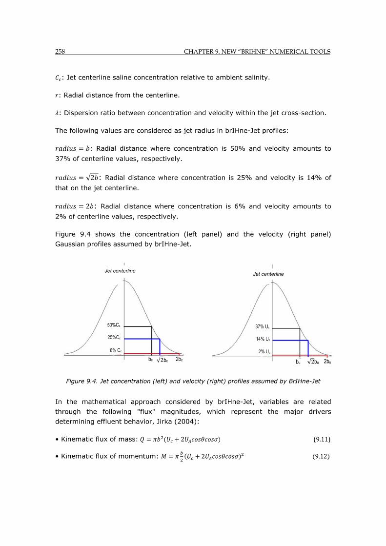
258 CHAPTER 9. NEW “BRIHNE” NUMERICAL TOOLS
: Jet centerline saline concentration relative to ambient salinity.
: Radial distance from the centerline.
: Dispersion ratio between concentration and velocity within the jet cross-section.
The following values are considered as jet radius in brIHne-Jet profiles:
: Radial distance where concentration is 50% and velocity amounts to
37% of centerline values, respectively.
√2 : Radial distance where concentration is 25% and velocity is 14% of
that on the jet centerline.
2 : Radial distance where concentration is 6% and velocity amounts to
2% of centerline values, respectively.
Figure 9.4 shows the concentration (left panel) and the velocity (right panel)
Gaussian profiles assumed by brIHne-Jet.
Figure 9.4. Jet concentration (left) and velocity (right) profiles assumed by BrIHne-Jet
In the mathematical approach considered by brIHne-Jet, variables are related
through the following "flux" magnitudes, which represent the major drivers
determining effluent behavior, Jirka (2004):
• Kinematic flux of mass: 2 (9.11)
• Kinematic flux of momentum: 2 ² 9.12
2% Uc
37% Uc
Uc
2bu
14% Uc
√2bu bu
6% Cc
50%Cc
Cc
25%Cc
2bc √2bc bc
Jet centerline Jet centerline
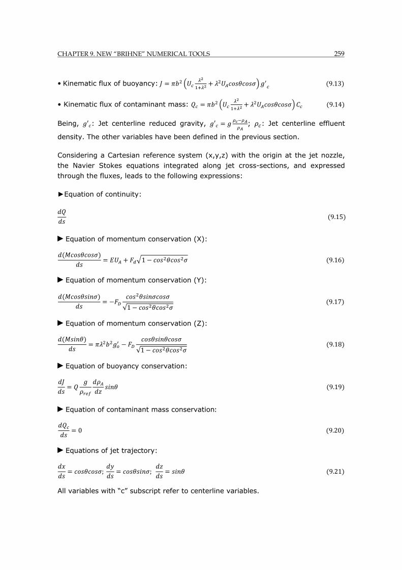
CHAPTER 9. NEW “BRIHNE” NUMERICAL TOOLS 259
• Kinematic flux of buoyancy: 9.13
• Kinematic flux of contaminant mass: 9.14
Being, : Jet centerline reduced gravity, ; : Jet centerline effluent
density. The other variables have been defined in the previous section.
Considering a Cartesian reference system (x,y,z) with the origin at the jet nozzle,
the Navier Stokes equations integrated along jet cross-sections, and expressed
through the fluxes, leads to the following expressions:
►Equation of continuity:
9.15
►Equation of momentum conservation (X):
1 9.16
►Equation of momentum conservation (Y):
√1 9.17
►Equation of momentum conservation (Z):
√1 9.18
►Equation of buoyancy conservation:
9.19
►Equation of contaminant mass conservation:
0 9.20
►Equations of jet trajectory:
; ; 9.21
All variables with “c” subscript refer to centerline variables.
260 CHAPTER 9. NEW “BRIHNE” NUMERICAL TOOLS
Turbulent Closure models
Previously to solve the differential equation system, closure models for the
turbulent entrainment rate ( ) and the ambient drag force ( ) terms are required.
The specification of these turbulent processes constitutes the “turbulence closure
problem” in the integral formulation.
In brIHne-Jet the entrainment ( ) of the ambient fluid into the turbulent jet
responds to the following equation:
2 2 | | 1 9.22
The left terms represents the transverse component, which mainly depends on the
excess of the centerline velocity ( ), the jet width ( ) and the empirical coefficients
( , , , ). The right term represents the azimuthal shear mechanisms, which are
overall influenced by the jet width ( ) and the ambient current velocity ( ).
Considering the jet radius as (radial distance where concentration is 50% and
velocity 37% of centerline values), the coefficients have the following values,
Jirka (2004):
0.055, pure jet coefficient.
0.6, pure plume coefficient.
0.055, pure wake coefficient.
0.5, advected plume coefficient.
In the streamwise shear component, the velocity excess ( ) above the ambient
velocity ( ) leads to instabilities in the form of axisymmetric ring vortices.
The mean entrainment occurs uniformly at the jet periphery.
In case of a stagnant environment ( 0) the azimuthal term is zero and the
transverse component of entrainment reduces to an equation depending on the jet
curvature ( ), the jet width ( ), centerline velocity ( ), the pure jet ( ) and the
pure plume ( ) coefficients.
The entrainment formula (equation 9.22) is derived from that originally proposed
by Priestley et al. (1955) for vertical buoyant jets
CHAPTER 9. NEW “BRIHNE” NUMERICAL TOOLS 261
2 9.23
This formula has been modified in brIHne-Jet (and in CORJET) by including an
additional term: “ " in order to consider the inclined negatively buoyant jet
curvature, Jirka (2004). However, this change does not result in a good agreement
with experimental data, as show in the validation of CORJET model carried out in
Chapter 4. Actually, discrepancies about 50% have been found in dilution rate
predictions obtained with CORJET. In order to get a better fit between integral
model approaches and experimental data regarding brine discharges, Panos et al.
(2008) proposed a modification of the pure jet and plume coefficients ( , ) value.
However, these coefficients have been scientifically accepted and experimentally
proved by Fischer et al. (1979), Papanicolaou et al. (1988) and Wang et al. (2002),
among others. Hence, a modification of these coefficients does not seem to be a
rigorous option and actually, results reveal that this modification does not improve
significantly the numerical prediction.
According to these facts, further research regarding the entrainment formula of
inclined negatively buoyant jets is required. Moreover, the entrainment formula and
the modeling equations need to be modified in order to consider the buoyant
instabilities that cause the extra spreading of the jet low boundary, invalidating the
self-similarity and Gaussian profile hypotheses (Chapter 7). Thanks to the PIV-PLIF
set of experimental data obtained in the present work, brIHne-Jet equations cab be
re-calibrated in order to consider these processes and to obtain a more reliable
prediction of brine jets.
The second turbulent closure model represents the drag force acting on the jet
element and caused by the presence of the ambient current, and is given by the
equation, Jirka (2004):
√2 1 9.24
Being , the coefficient of drag proposed by Jirka (2004): 1.3.
The nine governing equations of flux conservation and jet geometry (Equations
9.15 to 9.21), together with the equation of state, the Entrainment Equation (9.22)
and the drag force Equation (9.24) form a nine ordinary differential equation
system with nine unknown variables. Applying a fourth-order Runge-Kutta
algorithm, the system is numerically solved and the evolution of the nine jet
variables: , , , , , , , , is obtained by brIHe-Jet.
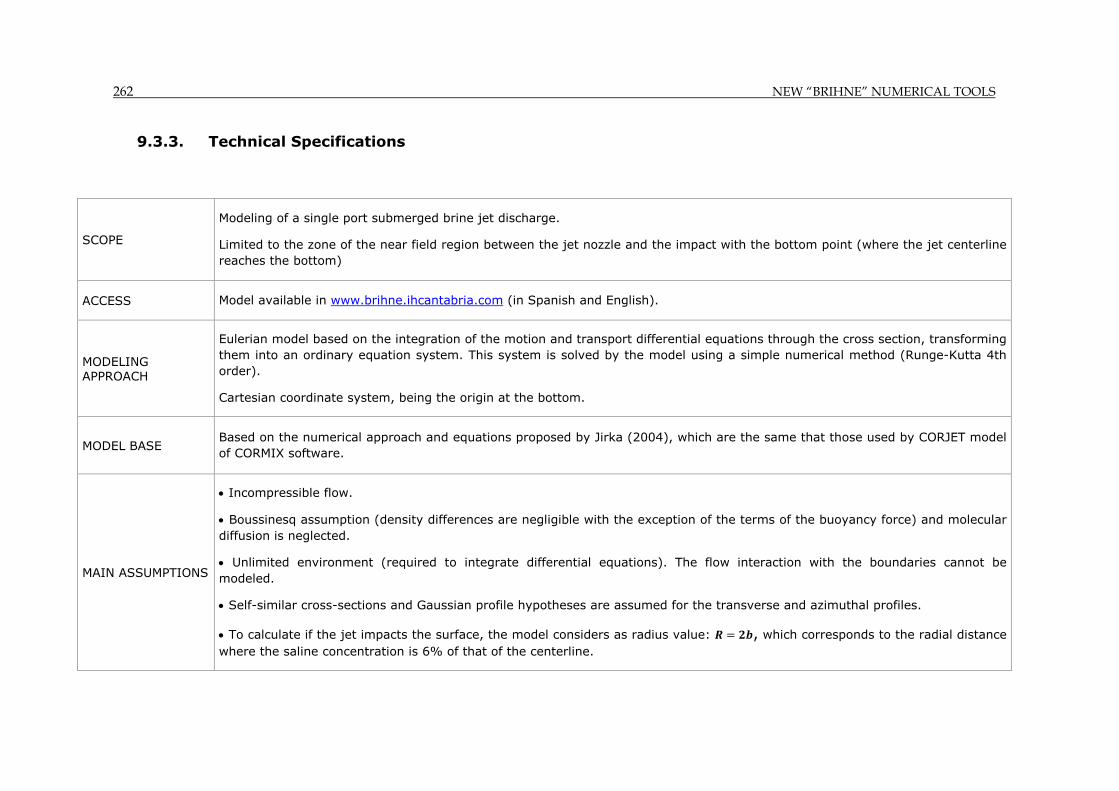
262 NEW “BRIHNE” NUMERICAL TOOLS
9.3.3. Technical Specifications
SCOPE
Modeling of a single port submerged brine jet discharge.
Limited to the zone of the near field region between the jet nozzle and the impact with the bottom point (where the jet centerline reaches the bottom)
ACCESS Model available in www.brihne.ihcantabria.com (in Spanish and English).
MODELING APPROACH
Eulerian model based on the integration of the motion and transport differential equations through the cross section, transforming them into an ordinary equation system. This system is solved by the model using a simple numerical method (Runge-Kutta 4th order).
Cartesian coordinate system, being the origin at the bottom.
MODEL BASE Based on the numerical approach and equations proposed by Jirka (2004), which are the same that those used by CORJET model of CORMIX software.
MAIN ASSUMPTIONS
Incompressible flow.
Boussinesq assumption (density differences are negligible with the exception of the terms of the buoyancy force) and molecular diffusion is neglected.
Unlimited environment (required to integrate differential equations). The flow interaction with the boundaries cannot be modeled.
Self-similar cross-sections and Gaussian profile hypotheses are assumed for the transverse and azimuthal profiles.
To calculate if the jet impacts the surface, the model considers as radius value: , which corresponds to the radial distance where the saline concentration is 6% of that of the centerline.
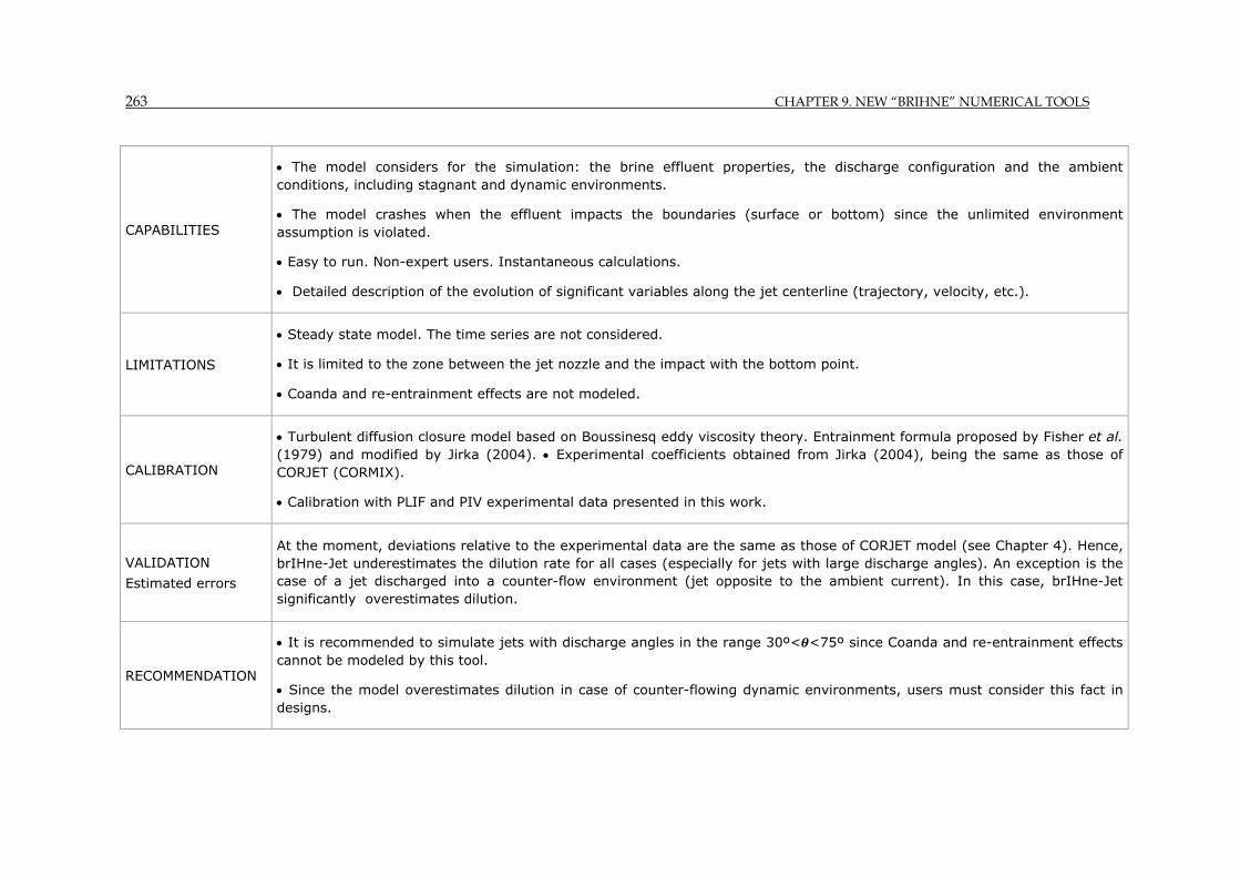
263 CHAPTER 9. NEW “BRIHNE” NUMERICAL TOOLS
CAPABILITIES
The model considers for the simulation: the brine effluent properties, the discharge configuration and the ambient conditions, including stagnant and dynamic environments.
The model crashes when the effluent impacts the boundaries (surface or bottom) since the unlimited environment assumption is violated.
Easy to run. Non-expert users. Instantaneous calculations.
Detailed description of the evolution of significant variables along the jet centerline (trajectory, velocity, etc.).
LIMITATIONS
Steady state model. The time series are not considered.
It is limited to the zone between the jet nozzle and the impact with the bottom point.
Coanda and re-entrainment effects are not modeled.
CALIBRATION
Turbulent diffusion closure model based on Boussinesq eddy viscosity theory. Entrainment formula proposed by Fisher et al. (1979) and modified by Jirka (2004). Experimental coefficients obtained from Jirka (2004), being the same as those of CORJET (CORMIX).
Calibration with PLIF and PIV experimental data presented in this work.
VALIDATION
Estimated errors
At the moment, deviations relative to the experimental data are the same as those of CORJET model (see Chapter 4). Hence, brIHne-Jet underestimates the dilution rate for all cases (especially for jets with large discharge angles). An exception is the case of a jet discharged into a counter-flow environment (jet opposite to the ambient current). In this case, brIHne-Jet significantly overestimates dilution.
RECOMMENDATION
It is recommended to simulate jets with discharge angles in the range 30º< <75º since Coanda and re-entrainment effects cannot be modeled by this tool.
Since the model overestimates dilution in case of counter-flowing dynamic environments, users must consider this fact in designs.

264 CHAPTER 9. NEW “BRIHNE” NUMERICAL TOOLS
9.3.4. Input data
The following variables are required as input data of the brIHne-Jet model:
: Average depth at discharge point.
: Receiving fluid (ambient) density.
: Receiving fluid (ambient) salinity.
: Receiving fluid (ambient) crossflow velocity.
: Horizontal angle between the jet and the environment crossflow.
: Effluent density.
: Effluent saline concentration.
: Port diameter.
: Port height.
: Jet discharge velocity.
: Jet discharge angle (vertical angle with respect to the bottom).
9.3.5. Model results
Once the model has been run, the following results are obtained:
Evolution of the following jet variables, from the jet port to the impact with
bottom point:
◦ Centerline coordinates ( , ).
◦ Centerline dilution ( ) and saline concentration ( ), curvature ( ), centerline
velocity ( ), centerline density ( ) and Densimetric Froude number ( ).
◦ Jet radius ( ), corresponding to the radial distance where concentration is 50%
and velocity is 37% of centerline and velocity concentration values, respectively.
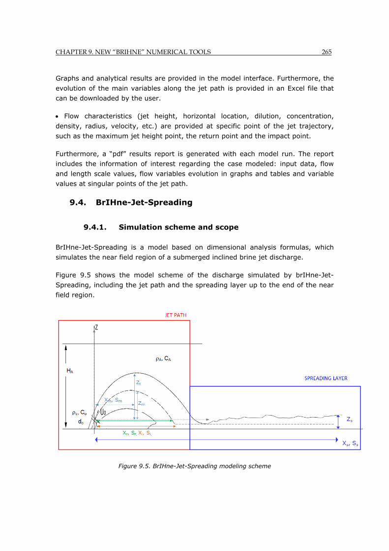
CHAPTER 9. NEW “BRIHNE” NUMERICAL TOOLS 265
Graphs and analytical results are provided in the model interface. Furthermore, the
evolution of the main variables along the jet path is provided in an Excel file that
can be downloaded by the user.
Flow characteristics (jet height, horizontal location, dilution, concentration,
density, radius, velocity, etc.) are provided at specific point of the jet trajectory,
such as the maximum jet height point, the return point and the impact point.
Furthermore, a “pdf” results report is generated with each model run. The report
includes the information of interest regarding the case modeled: input data, flow
and length scale values, flow variables evolution in graphs and tables and variable
values at singular points of the jet path.
9.4. BrIHne-Jet-Spreading
9.4.1. Simulation scheme and scope
BrIHne-Jet-Spreading is a model based on dimensional analysis formulas, which
simulates the near field region of a submerged inclined brine jet discharge.
Figure 9.5 shows the model scheme of the discharge simulated by brIHne-Jet-
Spreading, including the jet path and the spreading layer up to the end of the near
field region.
Figure 9.5. BrIHne-Jet-Spreading modeling scheme
266 CHAPTER 9. NEW “BRIHNE” NUMERICAL TOOLS
Where:
Variables regarding the receiving fluid (environment):
: Average depth at the discharge point; : Receiving fluid (ambient) salinity; :
Receiving fluid (ambient) density.
Variables regarding the brine effluent:
: Effluent density; : Effluent saline concentration.
Variables related to the discharge design:
: Port (nozzle) diameter; : Initial discharge angle; : Port (nozzle) height;
: Initial discharge velocity.
Flow parameters at singular points of the jet path:
, , , : Maximum rise height (upper edge height), centerline vertical location,
horizontal location and dilution at the jet centerline peak.
, : Centerline horizontal location (distance from the nozzle) and centerline
dilution at the return point.
, : Centerline horizontal location and centerline dilution at the impact with
bottom point.
, , , : Horizontal location, layer thickness, centerline dilution and centerline
velocity at the end of the spreading layer (end of the near field region and
beginning of the far field region).
9.4.2. Governing equations approach
BrIHne-Jet-Spreading applies dimensional analysis formulas, including the variables
with greater influence on the processes are considered, while those with less
influence are held constant, reducing the number of independent variables under
consideration.
Dimensional analysis for round jets sets up that, for a specific initial jet discharge
angle ( ), the variables of interest mainly depend on the port diameter ( ), the
Densimetric Froude number ( ) and the initial discharge angle ( ), Fisher et al.
(1979), Roberts et al. (1997):
CHAPTER 9. NEW “BRIHNE” NUMERICAL TOOLS 267
For a specific
, and
,
; ; ; ; ; (9.25)
Being:
“j” subscript represents the different locations along the jet path.
: Flow centerline horizontal location (distance from the origin), for each “j”
trajectory position.
: Flow centerline vertical location (distance from the mouth), for each “j”
trajectory position. This coordinate can be referred to the concentration axis ( ) or
to the velocity axis (Z ).
: Axis length for each “j” axis position ( , ). Similarly, it can be referred to the
concentration axis ( ) or to the velocity axis ( ).
: Centerline dilution at each concentration axis “j” position ( , ). The centerline
dilution represents the minimum dilution values of cross-sections.
: Jet radius for each “j” axis position along the jet trajectory. Along the spreading
layer trajectory, represents the layer thickness. This variable can be referred to
the radius and thickness obtained from the concentration fields ( ) or from the
velocity fields ( ).
: Centerline velocity at each “j” position along the flow trajectory. The centerline
velocity represents the maximum velocity values of cross-sections.
: For a specific discharge angle ( ), it represents the dimensional analysis
coefficients for each “ ” variable, at each “j” location of the flow trajectory.
The experimental coefficients values have been obtained, from each variable
and discharge angle case, from the PIV and PLIF experimental tests presented in
this Thesis, according to the calibration procedure explained in section 9.4.6.
From the previous variables, other dependent variables have been obtained
applying the following expressions:
268 CHAPTER 9. NEW “BRIHNE” NUMERICAL TOOLS
9.26
9.27
∆∆
9.28
; 9.29
Being:
: Centerline concentration at each “j” location along the flow trajectory. Centerline
represents the maximum concentration values of the cross-sections.
: Centerline density at each “j” location along the flow trajectory.
: Centerline inclination relative to the bottom at each “j” location along the flow
trajectory.
: Vertical component of the centerline velocity at each “j” location along the flow
trajectory.
: Horizontal component of the centerline velocity at each “j” location along the
flow trajectory.
9.4.3. Transverse profiles
9.4.3.1. Jet transverse profile
According to that explained in Chapters 6 and 7, inclined negatively buoyant jets,
such as those of brine discharges, present special features that make them diverge
from the typical behavior of a neutral non-inclined jet. One of these features is the
lower edge extra widening caused by the buoyancy-induced instabilities described
in detail in Chapter 7. The unusual spreading of the jet lower boundary invalidates
the self-similarity and Gaussian profiles hypotheses in this type of jets, except for
sections very close to the nozzle. Furthermore, this feature influences the mixing
processes, increasing the entrainment of the surrounding fluid into the effluent and,
hence, the dilution rate. Therefore, the jet centerlines trajectory, especially the
concentration axis, is modified and does not follow the expected trajectory.
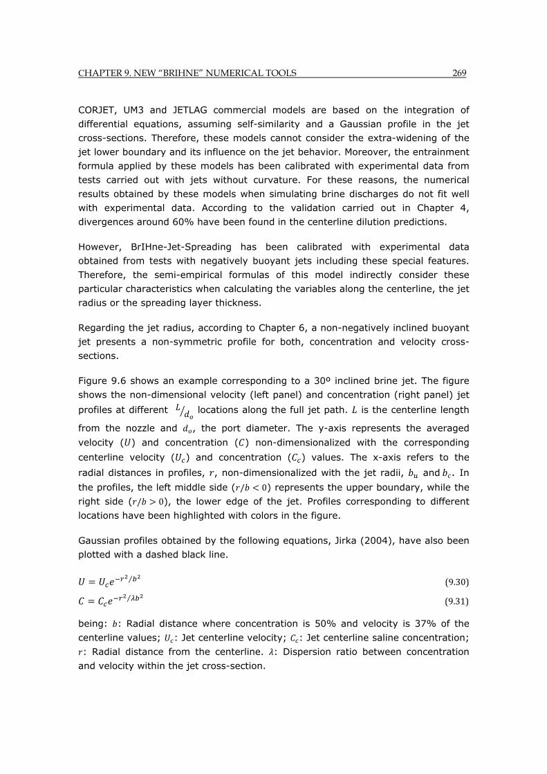
CHAPTER 9. NEW “BRIHNE” NUMERICAL TOOLS 269
CORJET, UM3 and JETLAG commercial models are based on the integration of
differential equations, assuming self-similarity and a Gaussian profile in the jet
cross-sections. Therefore, these models cannot consider the extra-widening of the
jet lower boundary and its influence on the jet behavior. Moreover, the entrainment
formula applied by these models has been calibrated with experimental data from
tests carried out with jets without curvature. For these reasons, the numerical
results obtained by these models when simulating brine discharges do not fit well
with experimental data. According to the validation carried out in Chapter 4,
divergences around 60% have been found in the centerline dilution predictions.
However, BrIHne-Jet-Spreading has been calibrated with experimental data
obtained from tests with negatively buoyant jets including these special features.
Therefore, the semi-empirical formulas of this model indirectly consider these
particular characteristics when calculating the variables along the centerline, the jet
radius or the spreading layer thickness.
Regarding the jet radius, according to Chapter 6, a non-negatively inclined buoyant
jet presents a non-symmetric profile for both, concentration and velocity cross-
sections.
Figure 9.6 shows an example corresponding to a 30º inclined brine jet. The figure
shows the non-dimensional velocity (left panel) and concentration (right panel) jet
profiles at different locations along the full jet path. is the centerline length
from the nozzle and , the port diameter. The y-axis represents the averaged
velocity ( ) and concentration ( ) non-dimensionalized with the corresponding
centerline velocity ( ) and concentration ( ) values. The x-axis refers to the
radial distances in profiles, , non-dimensionalized with the jet radii, and . In
the profiles, the left middle side ( / 0) represents the upper boundary, while the
right side ( / 0), the lower edge of the jet. Profiles corresponding to different
locations have been highlighted with colors in the figure.
Gaussian profiles obtained by the following equations, Jirka (2004), have also been
plotted with a dashed black line.
⁄ (9.30)
⁄ (9.31)
being: : Radial distance where concentration is 50% and velocity is 37% of the
centerline values; : Jet centerline velocity; : Jet centerline saline concentration;
: Radial distance from the centerline. : Dispersion ratio between concentration
and velocity within the jet cross-section.
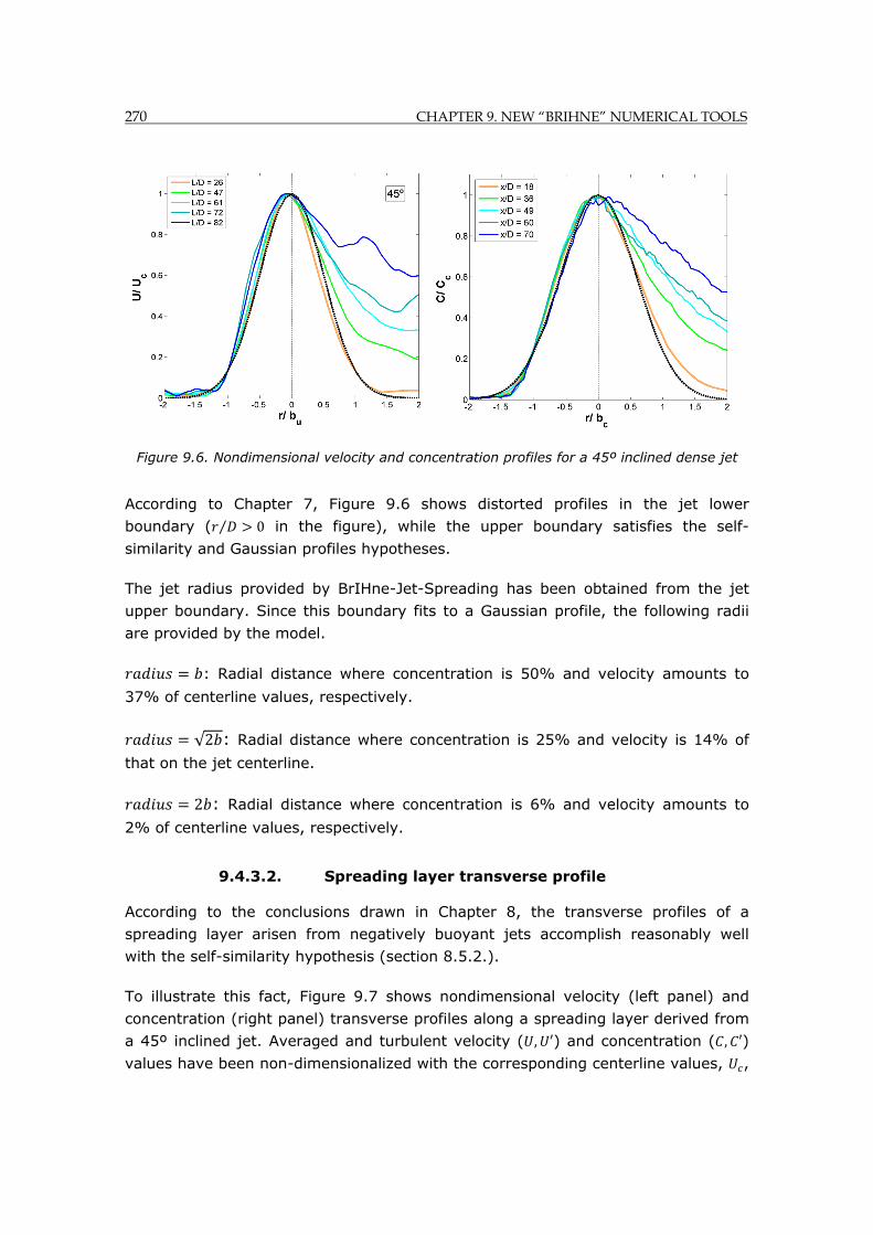
270 CHAPTER 9. NEW “BRIHNE” NUMERICAL TOOLS
Figure 9.6. Nondimensional velocity and concentration profiles for a 45º inclined dense jet
According to Chapter 7, Figure 9.6 shows distorted profiles in the jet lower
boundary ( ⁄ 0 in the figure), while the upper boundary satisfies the self-
similarity and Gaussian profiles hypotheses.
The jet radius provided by BrIHne-Jet-Spreading has been obtained from the jet
upper boundary. Since this boundary fits to a Gaussian profile, the following radii
are provided by the model.
: Radial distance where concentration is 50% and velocity amounts to
37% of centerline values, respectively.
√2 : Radial distance where concentration is 25% and velocity is 14% of
that on the jet centerline.
2 : Radial distance where concentration is 6% and velocity amounts to
2% of centerline values, respectively.
9.4.3.2. Spreading layer transverse profile
According to the conclusions drawn in Chapter 8, the transverse profiles of a
spreading layer arisen from negatively buoyant jets accomplish reasonably well
with the self-similarity hypothesis (section 8.5.2.).
To illustrate this fact, Figure 9.7 shows nondimensional velocity (left panel) and
concentration (right panel) transverse profiles along a spreading layer derived from
a 45º inclined jet. Averaged and turbulent velocity ( , ) and concentration ( , )
values have been non-dimensionalized with the corresponding centerline values, ,
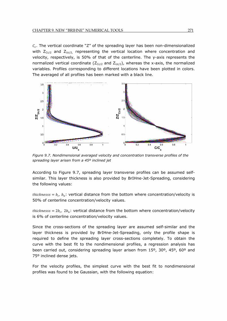
CHAPTER 9. NEW “BRIHNE” NUMERICAL TOOLS 271
. The vertical coordinate “Z” of the spreading layer has been non-dimensionalized
with ZCc/2 and ZUc/2, representing the vertical location where concentration and
velocity, respectively, is 50% of that of the centerline. The y-axis represents the
normalized vertical coordinate (ZCc/2 and ZUc/2), whereas the x-axis, the normalized
variables. Profiles corresponding to different locations have been plotted in colors.
The averaged of all profiles has been marked with a black line.
Figure 9.7. Nondimensional averaged velocity and concentration transverse profiles of the spreading layer arisen from a 45º inclined jet
According to Figure 9.7, spreading layer transverse profiles can be assumed self-
similar. This layer thickness is also provided by BrIHne-Jet-Spreading, considering
the following values:
, : vertical distance from the bottom where concentration/velocity is
50% of centerline concentration/velocity values.
2 , 2 : vertical distance from the bottom where concentration/velocity
is 6% of centerline concentration/velocity values.
Since the cross-sections of the spreading layer are assumed self-similar and the
layer thickness is provided by BrIHne-Jet-Spreading, only the profile shape is
required to define the spreading layer cross-sections completely. To obtain the
curve with the best fit to the nondimensional profiles, a regression analysis has
been carried out, considering spreading layer arisen from 15º, 30º, 45º, 60º and
75º inclined dense jets.
For the velocity profiles, the simplest curve with the best fit to nondimensional
profiles was found to be Gaussian, with the following equation:
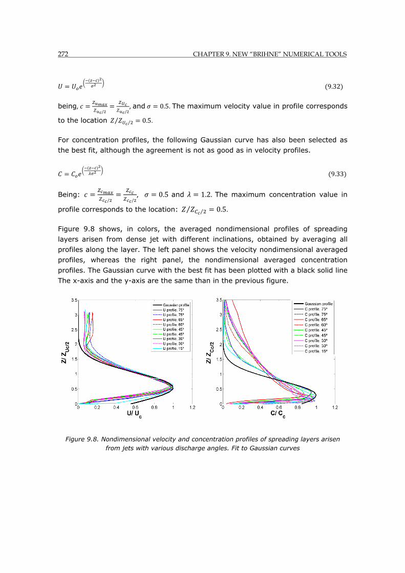
272 CHAPTER 9. NEW “BRIHNE” NUMERICAL TOOLS
9.32
being, / /
, and 0.5. The maximum velocity value in profile corresponds
to the location ⁄ 0.5⁄ .
For concentration profiles, the following Gaussian curve has also been selected as
the best fit, although the agreement is not as good as in velocity profiles.
9.33
Being: / /
, 0.5 and 1.2. The maximum concentration value in
profile corresponds to the location: ⁄ 0.5⁄ .
Figure 9.8 shows, in colors, the averaged nondimensional profiles of spreading
layers arisen from dense jet with different inclinations, obtained by averaging all
profiles along the layer. The left panel shows the velocity nondimensional averaged
profiles, whereas the right panel, the nondimensional averaged concentration
profiles. The Gaussian curve with the best fit has been plotted with a black solid line
The x-axis and the y-axis are the same than in the previous figure.
Figure 9.8. Nondimensional velocity and concentration profiles of spreading layers arisen from jets with various discharge angles. Fit to Gaussian curves

CHAPTER 9. NEW “BRIHNE” NUMERICAL TOOLS 273
9.4.4. Coupling conditions for a far field model
The flow characteristics of the spreading layer at the end of the near field region
represent the coupling flow conditions for a hydrodynamic model to simulate the
behavior at the far field region.
The coupling conditions provided by BrIHne-Jet-Spreading are the velocity and
concentration transverse profiles of the spreading layer at the end of the near field
region. Assuming self-similar cross-sections and providing the thickness and shape
of the velocity and concentration transverse profiles, the flow conditions to use as
input data in a far field model are defined.

274 CHAPTER 9. NEW “BRIHNE” NUMERICAL TOOLS
9.4.5. Technical specifications
SCOPE
Simulation of a submerged and inclined single port brine jet discharge.
Modeling of the whole near field region, including the jet path and the spreading layer formed after the impact with bottom point.
ACCESS Available in www.brihne.ihcantabria.com, in Spanish and English.
MODELING APPROACH
Based on dimensional analysis formulas to characterize negatively buoyant jets and spreading layers.
Formulas have been calibrated with the experimental data obtained by the non-intrusive PIV-PLIF techniques described in the present work (Chapters 5 to 8).
MAIN ASSUMPTIONS
Fully turbulent flow, viscous forces are negligible.
For Reynolds numbers higher than 2000 and Densimetric Froude numbers higher than 20, the flow can be assumed fully developed and the source volume flux being negligible. For these conditions, dimensional analysis can be applied to characterize the flow.
Geometrical variables, flux velocity and dilution, according to dimensional analysis, are assumed to only depend on the Densimetric Froude Number ( , the port diameter ( ) and the discharge velocity ( ).
Applying the criterion proposed by Roberts et al. (1997), the end of the near field region is considered to be reached at a distance Xs/(doFrd)=9 from the jet nozzle. For this location, the turbulent component of variables is negligible relative to the averaged component.
Model considers a zone of flow establishment (ZOFE) close to the mouth, according to the criterion of Jirka (2004)

CHAPTER 9. NEW “BRIHNE” NUMERICAL TOOLS 275
CAPABILITIES
BrIHne-Jet-Spreading simulates the whole near field region of a brine discharge against CORJET, UM3 and JETLAG commercial models, which only model the jet path up to the point where the jet impacts the bottom.
BrIHne-Jet-Spreading provides the flow characteristics at the end of the near field region. This allows establishing the coupling conditions to be used as input data in a far field model. Since, it is a bi-dimensional model, these coupling conditions are the velocity and concentration transverse profiles of the spreading layer at the end of the near field region.
The model simulates jets with different discharge angles, covering the range values (15° 75°) used in actual desalination plants.
Results include not only the flow characteristics at specific points but also the continuous characterization of the flow behavior along the trajectory from the discharge point up to the end of the near field region.
Variables characterizing the hydrodynamic and mixing processes are provided by the modeling.
LIMITATIONS
The far field region is not modeled.
Flat and horizontal bottom.
Stagnant and homogeneous environment.
Steady state model. Time series are not considered. Each run simulates a specific scenario.
The impact with the surface or with lateral boundaries is not modeled.
Modeling is limited to the following specific discharge angles: 15°, 30°, 45°, 60° and 75°.

276 CHAPTER 9. NEW “BRIHNE” NUMERICAL TOOLS
CALIBRATION BrIHne-Jet-Spreading has been calibrated with the experimental data obtained from the test carried out in the Environmental Hydraulics Institute using non-intrusive optical techniques: PIV (Particle image Velocimetry) and PLIF (Planar Laser Induced Fluorescence), described in Chapters 5 to 8. The calibration procedure is briefly explained in the following sections.
VALIDATION The model fits very well with experimental data published by other authors, as explained in following sections.
RECOMMENDAT.
If the flow wants to be characterized for a discharge angle in-between those simulated by the model, 15°, 30°, 45°, 60° and 75°, a linear interpolation can be made at the specific points of the flow trajectory: maximum rise height, return point, impact point and end of the spreading layer. For the interpolation, the proportional averaged between values corresponding to the immediately higher and lower discharge angle of that desired, is recommended to be calculated
BRIHne-Jet-Spreading is not recommended to be used for jets with an initial Densimetric Froude Number lower than 15. Furthermore, it never must be used if the jet Densimetric Froude number is lower than 10, since the dimensional analysis assumptions considered are no longer valid.
CHAPTER 9. NEW “BRIHNE” NUMERICAL TOOLS 277
9.4.6. Input data
The following variables are required as input data of brIHne-Jet-Spreading model:
: Average depth at discharge point.
: Receiving fluid (ambient) density.
: Receiving fluid (ambient) salinity.
: Brine effluent density.
: Brine saline concentration.
: Port diameter.
: Discharge velocity.
: Port height.
: Discharge angle relative to bottom.
9.4.7. Model results
Once the model has been run, the following results are obtained:
Evolution of the variables, from the jet port to the end of the near field region:
- Concentration (X , Z ) and velocity (X , Z ) flow centerline trajectory and the corresponding centerline lengths, (L ) and (L ), respectively.
- Centerline dilution (S), saline concentration (C), density (ρ), velocity (U) and its vertical and horizontal components (U , U ), etc., along the flow trajectory.
- Jet radius and spreading layer thickness along the flow trajectory, corresponding to the concentration flow field (b ) and the velocity flow field (b ).
These results are presented graphically and analytically in the model interface.
Moreover, an Excel file with the analytical results is provided.
278 CHAPTER 9. NEW “BRIHNE” NUMERICAL TOOLS
Flow characteristics at singular points along the jet trajectory, such as the
maximum jet height point, the return point, the impact with bottom point and the
end of the near field region.
Velocity and concentration profiles of the spreading layer at the end of the near
field region, as coupling conditions with a far field model.
Moreover, a results report in “pdf” is generated with each model run. The report
includes the information of interest regarding the case modeled: input data, flow
and length scale values, flow variables evolution in graphs and tables, variables
value at singular point of the flow and velocity and concentration profiles at the end
of the near field region.
9.4.8. Calibration
BrIHne-Jet-Spreading has been calibrated with experimental data obtained by the
PIV and PLIF experimental data of the present work, described in Chapters 5 to 8.
Since brIHne-Jet-Spreading calibration coefficients have been obtained from tests
corresponding to actual negatively buoyant jet discharges, the special features of
this type of jets are considered in the model predictions.
Once obtained the averaged velocity and the concentration flow-fields of the brine
jet and spreading layer for every case tested, the calibration procedure of BrIHne-
Jet-Spreading can be summarized in the following main steps:
▪ For each case tested, the velocity and concentration centerlines have been
obtained from the averaged flow-fields. The evolution of the main flow variables
(concentration, dilution, velocity, density, etc.) has been calculated along these
axes up to the end of the near field region.
▪ Across planes perpendicular to the centerline, velocity and concentration profiles
have been defined for each test. From these profiles, the jet width and the
spreading layer thickness have been calculated from the jet nozzle up to the end of
the near field region.
▪ Applying dimensional analysis for negatively buoyant jets and spreading layers,
the coefficient values for the following dimensional analysis formulas have been
calculated for each point of the jet path and for each case tested:
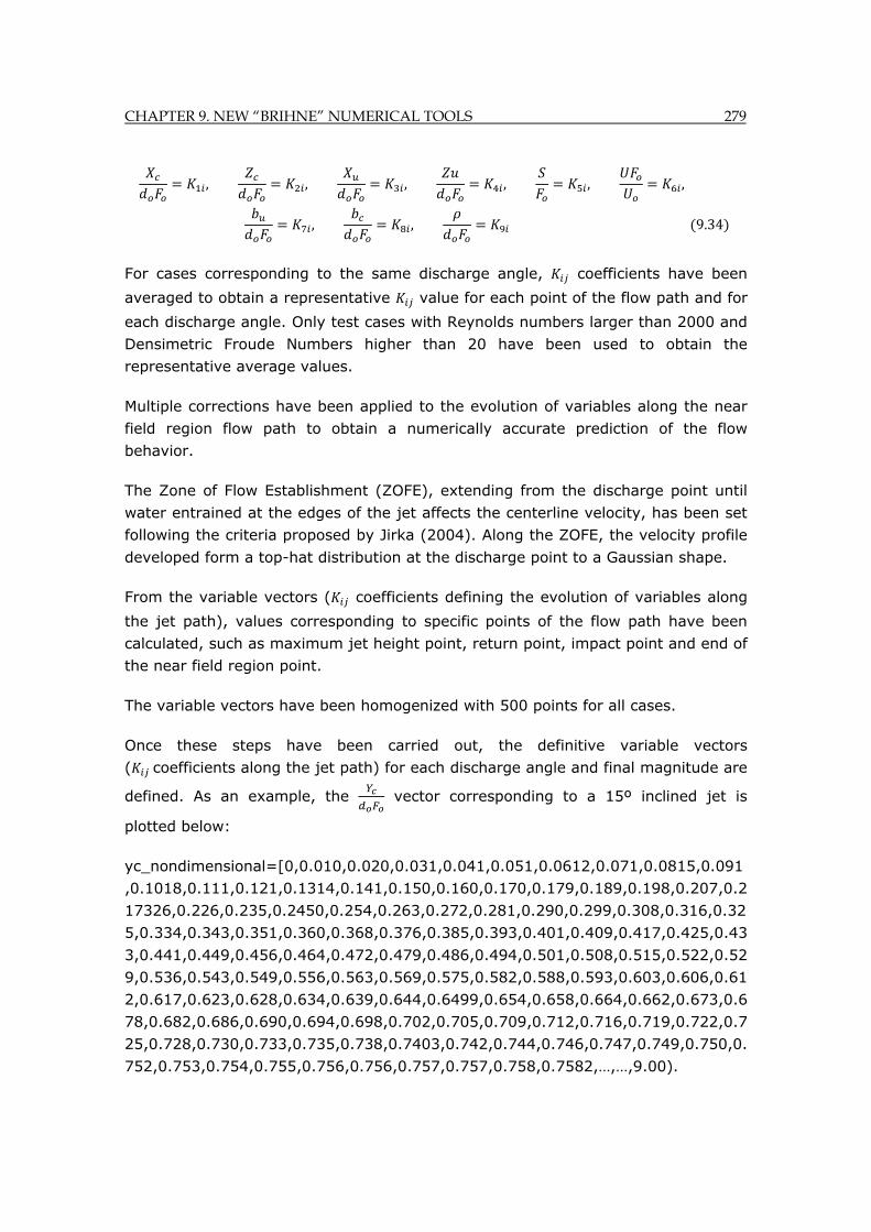
CHAPTER 9. NEW “BRIHNE” NUMERICAL TOOLS 279
, , , , , ,
, , 9.34
For cases corresponding to the same discharge angle, coefficients have been
averaged to obtain a representative value for each point of the flow path and for
each discharge angle. Only test cases with Reynolds numbers larger than 2000 and
Densimetric Froude Numbers higher than 20 have been used to obtain the
representative average values.
Multiple corrections have been applied to the evolution of variables along the near
field region flow path to obtain a numerically accurate prediction of the flow
behavior.
The Zone of Flow Establishment (ZOFE), extending from the discharge point until
water entrained at the edges of the jet affects the centerline velocity, has been set
following the criteria proposed by Jirka (2004). Along the ZOFE, the velocity profile
developed form a top-hat distribution at the discharge point to a Gaussian shape.
From the variable vectors ( coefficients defining the evolution of variables along
the jet path), values corresponding to specific points of the flow path have been
calculated, such as maximum jet height point, return point, impact point and end of
the near field region point.
The variable vectors have been homogenized with 500 points for all cases.
Once these steps have been carried out, the definitive variable vectors
( coefficients along the jet path) for each discharge angle and final magnitude are
defined. As an example, the vector corresponding to a 15º inclined jet is
plotted below:
yc_nondimensional=[0,0.010,0.020,0.031,0.041,0.051,0.0612,0.071,0.0815,0.091
,0.1018,0.111,0.121,0.1314,0.141,0.150,0.160,0.170,0.179,0.189,0.198,0.207,0.2
17326,0.226,0.235,0.2450,0.254,0.263,0.272,0.281,0.290,0.299,0.308,0.316,0.32
5,0.334,0.343,0.351,0.360,0.368,0.376,0.385,0.393,0.401,0.409,0.417,0.425,0.43
3,0.441,0.449,0.456,0.464,0.472,0.479,0.486,0.494,0.501,0.508,0.515,0.522,0.52
9,0.536,0.543,0.549,0.556,0.563,0.569,0.575,0.582,0.588,0.593,0.603,0.606,0.61
2,0.617,0.623,0.628,0.634,0.639,0.644,0.6499,0.654,0.658,0.664,0.662,0.673,0.6
78,0.682,0.686,0.690,0.694,0.698,0.702,0.705,0.709,0.712,0.716,0.719,0.722,0.7
25,0.728,0.730,0.733,0.735,0.738,0.7403,0.742,0.744,0.746,0.747,0.749,0.750,0.
752,0.753,0.754,0.755,0.756,0.756,0.757,0.757,0.758,0.7582,…,…,9.00).
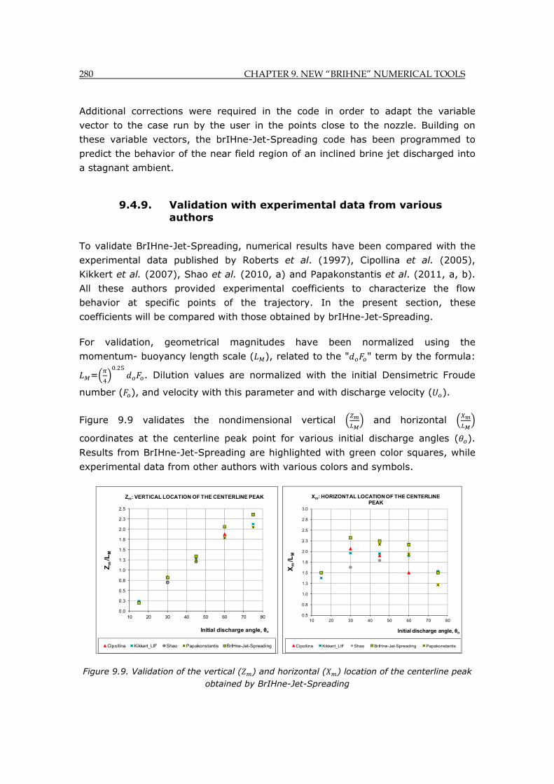
280 CHAPTER 9. NEW “BRIHNE” NUMERICAL TOOLS
Additional corrections were required in the code in order to adapt the variable
vector to the case run by the user in the points close to the nozzle. Building on
these variable vectors, the brIHne-Jet-Spreading code has been programmed to
predict the behavior of the near field region of an inclined brine jet discharged into
a stagnant ambient.
9.4.9. Validation with experimental data from various authors
To validate BrIHne-Jet-Spreading, numerical results have been compared with the
experimental data published by Roberts et al. (1997), Cipollina et al. (2005),
Kikkert et al. (2007), Shao et al. (2010, a) and Papakonstantis et al. (2011, a, b).
All these authors provided experimental coefficients to characterize the flow
behavior at specific points of the trajectory. In the present section, these
coefficients will be compared with those obtained by brIHne-Jet-Spreading.
For validation, geometrical magnitudes have been normalized using the
momentum- buoyancy length scale ( ), related to the " " term by the formula:
=.
. Dilution values are normalized with the initial Densimetric Froude
number ( ), and velocity with this parameter and with discharge velocity ( ).
Figure 9.9 validates the nondimensional vertical and horizontal
coordinates at the centerline peak point for various initial discharge angles ( ).
Results from BrIHne-Jet-Spreading are highlighted with green color squares, while
experimental data from other authors with various colors and symbols.
Figure 9.9. Validation of the vertical ( ) and horizontal ( ) location of the centerline peak obtained by BrIHne-Jet-Spreading
0.0
0.3
0.5
0.8
1.0
1.3
1.5
1.8
2.0
2.3
2.5
10 20 30 40 50 60 70 80
Zm
/LM
Initial discharge angle, θo
Zm: VERTICAL LOCATION OF THE CENTERLINE PEAK
Cipollina Kikkert_LIF Shao Papakonstantis BrIHne-Jet-Spreading
0.5
0.8
1.0
1.3
1.5
1.8
2.0
2.3
2.5
2.8
3.0
10 20 30 40 50 60 70 80
Xm
/LM
Initial discharge angle, θo
Xm: HORIZONTAL LOCATION OF THE CENTERLINE PEAK
Cipollina Kikkert_LIF Shao BrIHne-Jet-Spreading Papakonstantis
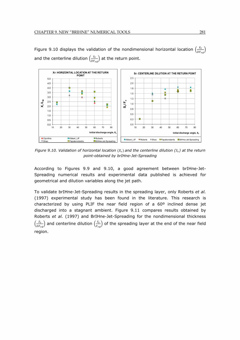
CHAPTER 9. NEW “BRIHNE” NUMERICAL TOOLS 281
Figure 9.10 displays the validation of the nondimensional horizontal location
and the centerline dilution at the return point.
Figure 9.10. Validation of horizontal location and the centerline dilution ( ) at the return point-obtained by brIHne-Jet-Spreading
According to Figures 9.9 and 9.10, a good agreement between brIHne-Jet-
Spreading numerical results and experimental data published is achieved for
geometrical and dilution variables along the jet path.
To validate brIHne-Jet-Spreading results in the spreading layer, only Roberts et al.
(1997) experimental study has been found in the literature. This research is
characterized by using PLIF the near field region of a 60º inclined dense jet
discharged into a stagnant ambient. Figure 9.11 compares results obtained by
Roberts et al. (1997) and BrIHne-Jet-Spreading for the nondimensional thickness
and centerline dilution of the spreading layer at the end of the near field
region.
0.0
0.5
1.0
1.5
2.0
2.5
3.0
3.5
4.0
4.5
5.0
10 20 30 40 50 60 70 80
Xr/L
M
Initial discharge angle, θo
Xr: HORIZONTAL LOCATION AT THE RETURN POINT
Cipollina Kikkert_LIF RobertsShao Papakonstantis BrIHne-Jet-Spreading
0.0
0.3
0.5
0.8
1.0
1.3
1.5
1.8
2.0
2.3
10 20 30 40 50 60 70 80S
r/ F
o
Initial discharge angle, θo
Sr: CENTERLINE DILUTION AT THE RETURN POINT
Kikkert_LIF Roberts Shao Papakonstantis BrIHne-Jet-Spreading
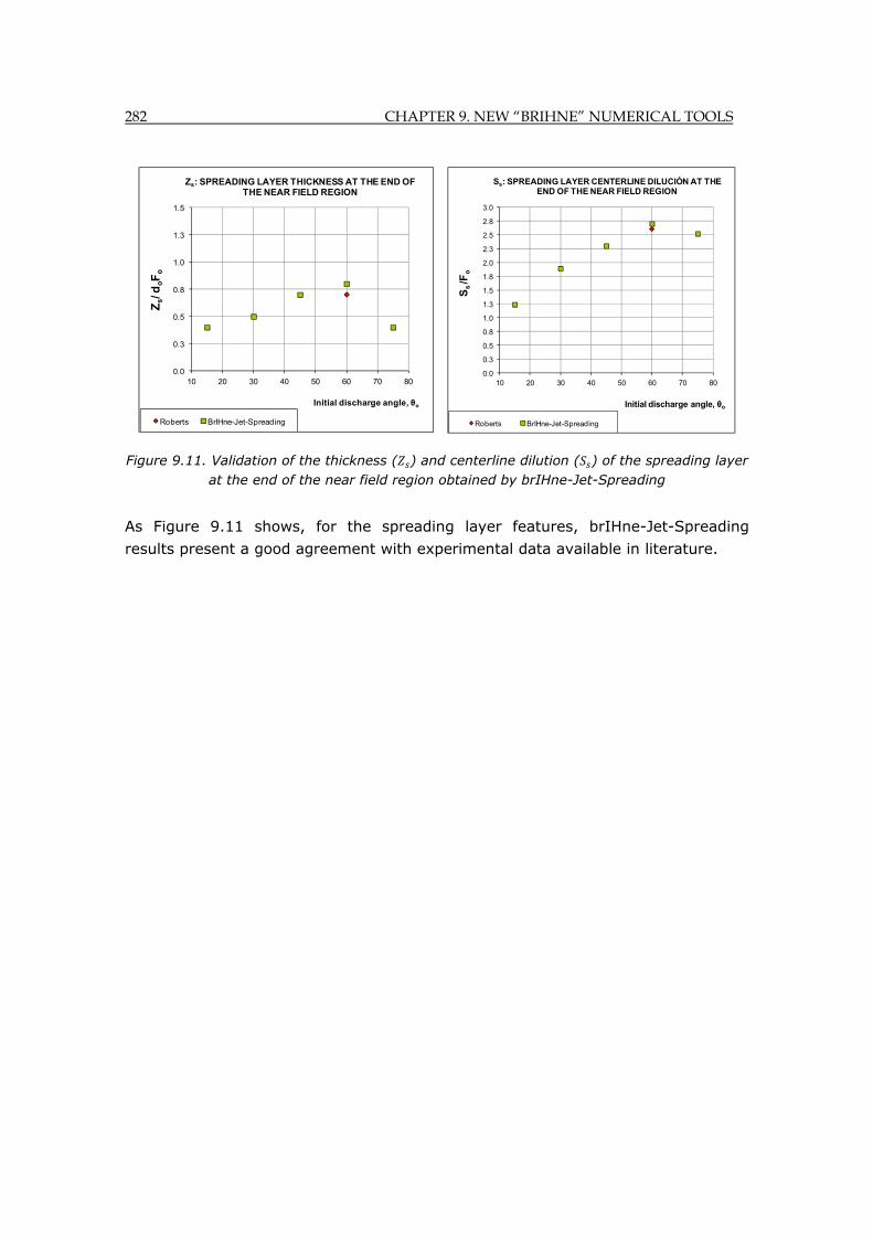
282 CHAPTER 9. NEW “BRIHNE” NUMERICAL TOOLS
Figure 9.11. Validation of the thickness ( ) and centerline dilution ( ) of the spreading layer at the end of the near field region obtained by brIHne-Jet-Spreading
As Figure 9.11 shows, for the spreading layer features, brIHne-Jet-Spreading
results present a good agreement with experimental data available in literature.
0.0
0.3
0.5
0.8
1.0
1.3
1.5
10 20 30 40 50 60 70 80
Zs/ d
oF
o
Initial discharge angle, θo
Zs: SPREADING LAYER THICKNESS AT THE END OF THE NEAR FIELD REGION
Roberts BrIHne-Jet-Spreading
0.0
0.3
0.5
0.8
1.0
1.3
1.5
1.8
2.0
2.3
2.5
2.8
3.0
10 20 30 40 50 60 70 80
Ss
/Fo
Initial discharge angle, θo
Ss: SPREADING LAYER CENTERLINE DILUCIÓN AT THE END OF THE NEAR FIELD REGION
Roberts BrIHne-Jet-Spreading
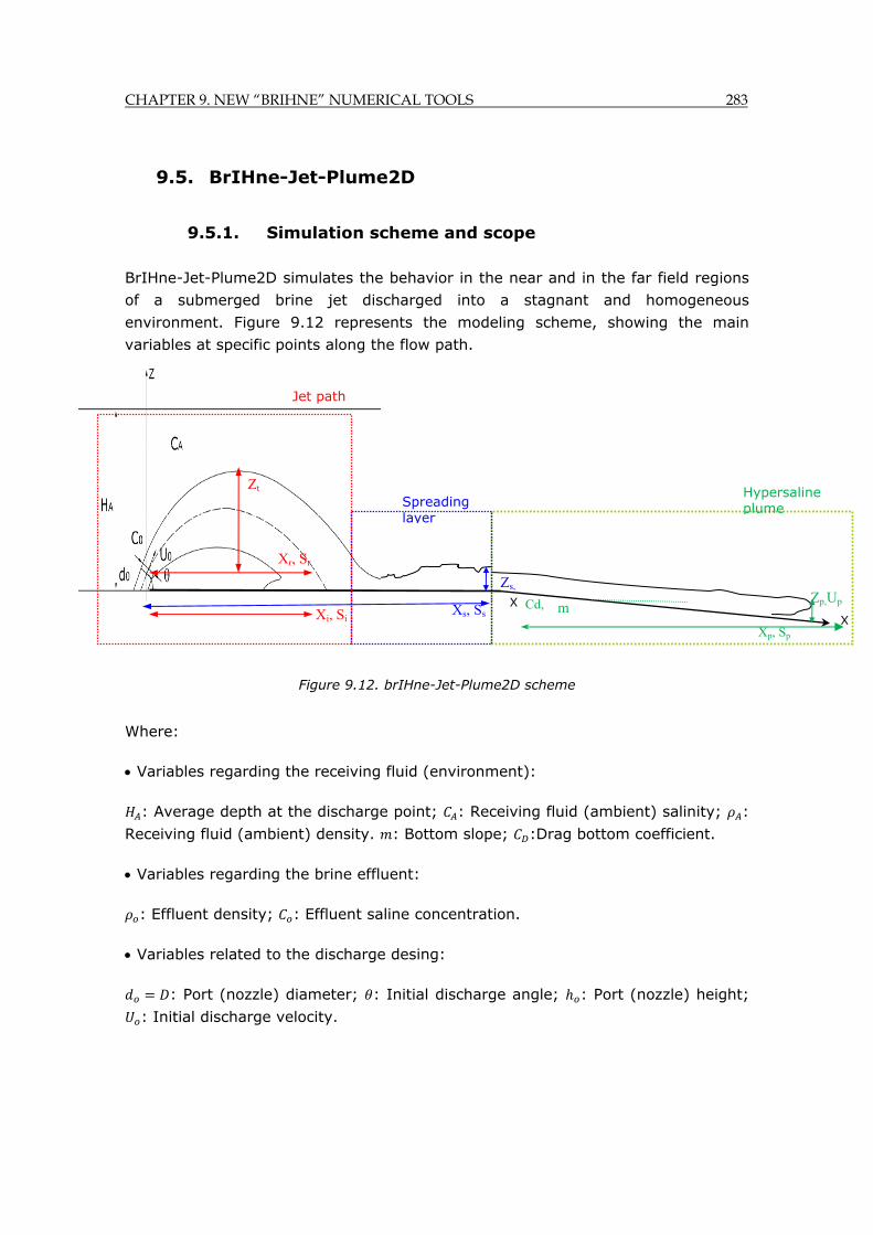
CHAPTER 9. NEW “BRIHNE” NUMERICAL TOOLS 283
9.5. BrIHne-Jet-Plume2D
9.5.1. Simulation scheme and scope
BrIHne-Jet-Plume2D simulates the behavior in the near and in the far field regions
of a submerged brine jet discharged into a stagnant and homogeneous
environment. Figure 9.12 represents the modeling scheme, showing the main
variables at specific points along the flow path.
Figure 9.12. brIHne-Jet-Plume2D scheme
Where:
Variables regarding the receiving fluid (environment):
: Average depth at the discharge point; : Receiving fluid (ambient) salinity; :
Receiving fluid (ambient) density. : Bottom slope; :Drag bottom coefficient.
Variables regarding the brine effluent:
: Effluent density; : Effluent saline concentration.
Variables related to the discharge desing:
: Port (nozzle) diameter; : Initial discharge angle; : Port (nozzle) height;
: Initial discharge velocity.
X
X Cd,
Xp, Sp
Zp,Up m
Zs,
Xs, Ss
Xr, Sr
Zt
Jet path
Xi, Si
Hypersaline plume Spreading
layer
284 CHAPTER 9. NEW “BRIHNE” NUMERICAL TOOLS
Flow parameters at singular points of the jet path:
, , , : Maximum rise height (upper edge height), centerline vertical location,
horizontal location and dilution at the jet centerline peak.
, : Centerline horizontal location (distance from the nozzle) and centerline
dilution at the return point.
, : Centerline horizontal location and centerline dilution at the impact with
bottom point.
, , , : Horizontal location, layer thickness, centerline dilution and centerline
velocity at the end of the spreading layer (end of the near field region and
beginning of the far field region).
, , , : Horizontal location, layer thickness, centerline dilution and centerline
velocity of the hypersaline plume (far field region).
9.5.2. Governing equations approach
Near field model
To predict the behavior of the jet brine discharge in the near field region (jet path
and spreading layer), BrIHne-Jet-Plume2D applies the same dimensional analysis
formulas as those used in brIHne-Jet-Spreading. These semi-empirical formulas
have been calibrated with the PIV and PLIF experimental data found in the
literature.
The conditions at the end of the near field region are obtained by the near field
region module of BrIHne-Jet-Plume2D, which carries out the coupling to the far
field region module by conserving the mass and the momentum flow fluxes.
Far field model
The module to simulate the behavior of the hypersaline plume typical of the far
field region is based on the integration of the plume differential equations across
sections, following the approach proposed by García. (1996). This approach
predicts the behavior of a gravity current flowing down on a sloping bottom in an
otherwise stagnant, less dense fluid. The model focuses on the steady dense layer
flow behind the gravity current initial front.
CHAPTER 9. NEW “BRIHNE” NUMERICAL TOOLS 285
The integral equations approach solved by brIHne-Jet-Spreading is analogous to
that originally set up by Ellison et al. (1959) for a dense layer, but in the present
approach, density variation is expressed trough the following buoyancy fraction
term:
∆ 9.35
The model assumes the Boussinesq hypothesis (density differences are negligible
except for the terms of the buoyancy force), a mild bottom slope (Sp<<1), a
stationary state, the Fick law, a similar viscosity for the dense layer and the
ambient fluid, the Reynolds decomposition and a hydrostatic pressure distribution
within the dense layer.
The governing equations are integrated along the plume vertical profile, assuming
self-similarity and a specific cross section shape. The resulting equations are
exposed below:
►Equation of mass conservation (buoyancy flux constant):
0 9.36
► Equation of continuity:
9.37
►Equation of momentum conservation in the direction of the mean motion:
12
9.38
Being:
: Plume average velocity.
: Plume thickness.
: Plume width (constant).
: Density fraction term.
, , : Initial values of these terms.
: Bottom inclination.
286 CHAPTER 9. NEW “BRIHNE” NUMERICAL TOOLS
: Bottom slope
: Gravity term.
: Friction coefficient.
, : Shape factors to represent the non-uniformity of the density distribution. represents the extent of the dense layer concentration compared to the vertical extent of motion. The expressions of these terms are the following:
2 9.39
1 9.40
The value of these parameters has been experimentally obtained by various
authors. Ellison et al. (1959) found, for low Reynolds numbers, values of 0.20.3 and 0.6 0.9 for a plane two-dimensional density flow. For three-
dimensional currents, similar values were found by Alavian. (1986). For high
Reynolds numbers, Schlapfer et al. (1987) obtained: 0.6 1 and 0.9 1.1.
BrIHne-Jet-Plume2D assumes the values: 0.3 and 0.8, which are in the
range of the values proposed by these authors.
Combining the equations previously displayed and the Richardson number
expression, a two ordinary differential equation system is obtained, with two
unknown variables: the hypersaline plume thickness and the Richardson
number , corresponding to a stationary flow:
2 0.51
9.41
31 0.5
1 9.42
Being:
: Richardson number is the dimensionless number, which expresses the ratio of
potential energy to kinetic energy. It is related to the Froude number, being the
Froude number the reciprocal of the square root of the Richardson number (
1/ ).
9.43
CHAPTER 9. NEW “BRIHNE” NUMERICAL TOOLS 287
If the Richardson number is: 1, buoyancy is unimportant in the flow behavior.
If it is: 1, buoyancy is dominant (in the sense that there is an insufficient
kinetic energy to homogenize the fluids).
According to Koh (1981), the two-dimensional density current flowing down a
sloping surface attains a normal state a short distance downstream from the
source, which is characterized by a normal Richardson number ( ), following the
expression:
0.5 9.44
The entrainment value in the normal state ( ) presents the following expression:
9.45
Turbulent Closure models
To solve the differential equation system, closure models for the entrainment ( )
and friction ( ) terms are required since they constitute the “turbulence closure
problem” in the integral formulation.
Regarding the entrainment term ( ), the upper gravity current behaves as a free
shear region, where turbulence causes the above ambient fluid to entrain into the
hypersaline plume, diluting the brine and reducing the saline concentration.
The Entrainment formula used by brIHne-Jet-Plume2D is based on the eddy
viscosity hypothesis for a gravity current, relating the water volume entrained with
the Richardson number. For high Richardson number values ( 10), the friction
force becomes significant and requires to be considered in the entrainment
expression. There are multiple formulas for the entrainment proposed by different
authors and based on experimental tests. Figure 9.13 represents the evolution of
this variable ( ) against the Richardson Number ( ) for various expressions found
in the literature.
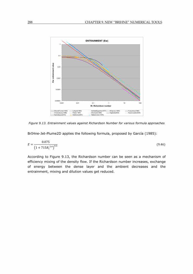
288 CHAPTER 9. NEW “BRIHNE” NUMERICAL TOOLS
Figure 9.13. Entrainment values against Richardson Number for various formula approaches
BrIHne-Jet-Plume2D applies the following formula, proposed by García (1985):
0.075
1 715 . . 9.46
According to Figure 9.13, the Richardson number can be seen as a mechanism of
efficiency mixing of the density flow. If the Richardson number increases, exchange
of energy between the dense layer and the ambient decreases and the
entrainment, mixing and dilution values get reduced.
ENTRAINMENT (Ew)
0.00001
0.0001
0.001
0.01
0.1
1
0.001 0.01 0.1 1 10 100
Ri: Richardson number
Ew
: e
ntr
ain
me
nt
va
lue
Ellison&Turner(1959) Lofquist(1960) Ashida&Egashira(1977) M:García (1993) Fukushima(1985)Christodoulou(1986) Parker 1987) Ghomeshi(1995) Haghiabi(2004) Karamzadeh(2004)
Kashefipour(2010) Dallimore(2001) Hebbert at al (1979)

CHAPTER 9. NEW “BRIHNE” NUMERICAL TOOLS 289
9.5.3. Technical specifications
SCOPE Modeling of the near field region (jet and spreading layer) and of the far field region (hypersaline plume) of a submerged single port jet brine discharge.
ACCESS Model available in: www.brihne.ihcantabria.com, in both, Spanish and English.
MODELING APPROACH
Dimensional analysis for modeling the near field region.
Integral differential equations to simulate the hypersaline plume of the far field region.
Coupling of the near and far field region by considering the mass and momentum fluxes conservation
MAIN ASSUMPTIONS
Common assumption to the near and the far field region:
Steady state model. Time series are not considered.
Stagnant and homogeneous environment.
Boussinesq assumption: density is constant in all terms of the equation system except for the gravity terms.
Fully turbulent flow. Similar viscous terms of the brine effluent and the ambient fluid.
Near field region:
According to the dimensional analysis applied to predict the near field region behavior, the flow variables are assumed to only depend on the Densimetric Froude Number ( ), the port diameter ( ) and the discharge velocity ( ).
The end of the near field region is considered to be reached at a distance of Xs/ doFrd =9 from the jet nozzle, according to the criterion proposed by Roberts et al. (1997).
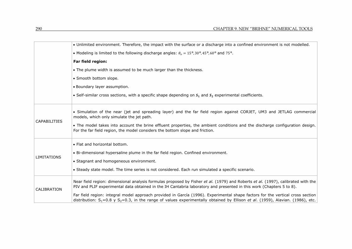
290 CHAPTER 9. NEW “BRIHNE” NUMERICAL TOOLS
Unlimited environment. Therefore, the impact with the surface or a discharge into a confined environment is not modelled.
Modeling is limited to the following discharge angles: 15°, 30°, 45°, 60° and 75°.
Far field region:
The plume width is assumed to be much larger than the thickness.
Smooth bottom slope.
Boundary layer assumption.
Self-similar cross sections, with a specific shape depending on and experimental coefficients.
CAPABILITIES
Simulation of the near (jet and spreading layer) and the far field region against CORJET, UM3 and JETLAG commercial models, which only simulate the jet path.
The model takes into account the brine effluent properties, the ambient conditions and the discharge configuration design. For the far field region, the model considers the bottom slope and friction.
LIMITATIONS
Flat and horizontal bottom.
Bi-dimensional hypersaline plume in the far field region. Confined environment.
Stagnant and homogeneous environment.
Steady state model. The time series is not considered. Each run simulated a specific scenario.
CALIBRATION
Near field region: dimensional analysis formulas proposed by Fisher et al. (1979) and Roberts et al. (1997), calibrated with the PIV and PLIF experimental data obtained in the IH Cantabria laboratory and presented in this work (Chapters 5 to 8).
Far field region: integral model approach provided in García (1996). Experimental shape factors for the vertical cross section distribution: S1=0.8 y S2=0.3, in the range of values experimentally obtained by Ellison et al. (1959), Alavian. (1986), etc.

CHAPTER 9. NEW “BRIHNE” NUMERICAL TOOLS 291
Entrainment formula proposed by García (1985). The far field approximation will be re-calibrated with new experimental data obtained by non-intrusive optical techniques in the Environmental Hydraulics Institute (IH Cantabria).
VALIDATION Results corresponding to the near field region (same as obtained by brIHne-Jet-Spreading) have been validated with experimental data found in the literature.
RECOMMENDAT.
If the flow wants to be characterized for a discharge angle in-between those simulated by the model ( 15°, 30°, 45°, 60° and 75°), the values at specific points of the flow trajectory (the maximum centerline peak point, the return point, the impact point and the end of the spreading layer) can be interpolated by averaging values corresponding to the immediately higher and lower discharge angle.
Model is not recommended for jets with an initial Densimetric Froude Number lower than 15, and it never must be used for Densimetric Froude number lower tan 10, since the hypothesis assumed to apply the dimensional analysis formulas becomes non-valid for that case.
Since the far field model does not consider the ambient current effect and requires further calibration, for the moment it is recommended considering its results as a preliminary estimation of the brine effluent behavior in the far field region.

292 CHAPTER 9. NEW “BRIHNE” NUMERICAL TOOLS
9.5.4. Input data
The following variables are required as input data of the model:
: Average depth at discharge point.
: Receiving fluid (environment) density.
: Receiving fluid (environment) salinity.
: Effluent density.
: Effluent saline concentration.
: Port (nozzle) diameter.
: Port (nozzle) height.
: Jet discharge velocity.
: Jet discharge angle (vertical angle with respect to the bottom).
: Bottom slope.
: Drag (friction) bottom coefficient.
The initial Densimetric Froude number is obtained by the formula:
9.5.5. Results
The following results are obtained once the model is run:
Variables value characterizing the flow at specific points of the near field region
trajectory: the maximum height point, the return point, the impact point and the
spreading layer at the end of the near field region.
Variables evolution along the hypersaline plume in the far field region up to the
distance of study chosen by the model user: Hypersaline plume thickness ( ),
centerline dilution ( ), saline concentration ( ), density ( ), velocity ( ), flow
rate ( ) and Richardson Number ( ), etc., along the flow trajectory.
These results are presented in the result model interface graphically and
analytically. Moreover, an Excel file with the analytical results and a “pdf” results

CHAPTER 9. NEW “BRIHNE” NUMERICAL TOOLS 293
report is generated with each model run. The report includes the information of
interest regarding the case modeled: input data, flow and length scale values, flow
variables evolution in graphs and tables, variables value at singular point of the
flow and velocity and concentration profiles at the end of the near field region.
9.6. A web based application for end-users
In order to make “brIHne” tools useful in actual desalination plant projects, they
have been made available online to designers and end-users through the website:
www.brihne.ihcantabria.com, in both, Spanish and English. As an example, Figures
9.14 and 9.15 show the interface and the result report obtained by running the
brIHne-Jet-Spreading, in Spanish.
Figure 9.14. BrIHne-Jet-Spreading model interface
Table with recommended input data
Technical Specifications
Warning file
Load input data
Model running Save input data
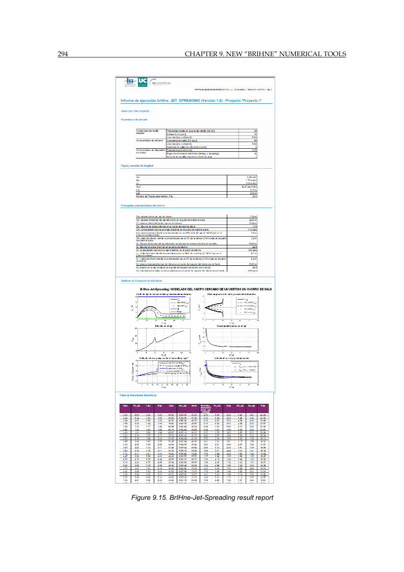
294 CHAPTER 9. NEW “BRIHNE” NUMERICAL TOOLS
Figure 9.15. BrIHne-Jet-Spreading result report
CHAPTER 9. NEW “BRIHNE” NUMERICAL TOOLS 295
9.7. Conclusions
“BrIHne” model have been developed as an alternative to commercial models, to
overcome their limitations and to have freely accessible online tools focused on
brine discharges.
The present chapter has described three “brIHne” tools to simulate submerged and
inclined brine jet discharges, using different mathematical approaches. These
models have been programmed with scientifically accepted governing equation
approaches and have been optimized providing an easy to use interface and a
results report after the model is run.
At the moment, brIHne-Jet results are the same as those obtained by the CORJET
commercial model, which is the most used by developers and environment
authorities. Since CORJET model numerical results do not fit well to experimental
data of dilution rate values, brIHne-Jet is being re-calibrated with PIV and PLIF
experimental data obtained in the IH Cantabria in the very near future.
BrIHne-Jet-Spreading can simulate the whole near field region of a brine jet
discharge with a high accurate reliability degree, thanks to the fact that it has been
re-calibrated with PIV and PLIF experimental data. Together with CORMIX1, it is, to
our knowledge, the only simulation tool available that models not only the jet path
but also the spreading layer. BrIHne-Jet-Spreading presents a higher agreement
with experimental data found in the literature than Cormix1.
Finally, brIHne-Jet-Plume presents the same accuracy degree of brIHne-Jet-
Spreading in the near field region prediction. It can also estimate the flow behavior
in the far field region.
All models are online available (www.brihneihcantabria.com), in both, Spanish and
English.

CHAPTER 9. NEW “BRIHNE” NUMERICAL TOOLS 296
CHAPTER 10. DEVELOPMENT A METHODOLOGY TO DESIGN BRINE DISCHARGES 297
Chapter 10. DEVELOPMENT OF A METHODOLOGY TO DESIGN BRINE DISCHARGES
Chapter 10 DEVELOPMENT OF A METHODOLOGY TO DESIGN BRINE DISCHARGES
Summary
As one of the main goals of the present Thesis, this chapter presents the
methodology developed to improve the design of brine discharges, intending to
reduce the potential negative impact of brine on the marine environment. The
methodology consists on five main steps to carry out the design and the
environmental impact assessment of brine discharges. Each step includes various
sub-steps, which are described in detail in the present chapter.
The methodological guide integrates the results, criteria and tools developed from
the partial objectives described in previous chapters: the critical assessment and
validation of commercial models (Chapters 3 and 4); the knowledge regarding
hydrodynamic and mixing processes involved in brine discharges (Chapters 5 to 8)
and the “brIHne” simulation tools developed as an alternative of commercial models
(Chapter 9). For a better understanding of the methodology proposed, a case study
is presented in this chapter, applying the methodologuical steps to an actual
desalination plant discharge.
With this guide, the design of brine discharges is expected to be improved, aiming
at make compatible the use of desalination as an important water resource with the
environmental protection of the marine areas.

298 CHAPTER 10. DEVELOPMENT A METHODOLOGY TO DESIGN BRINE DISCHARGES
10.1. Introduction
The increase of desalinated water production in Spain and the negative impact of
brine on marine ecosystems, together with the lack of legislation regarding brine
management and the lack of common criteria to design brine discharges, justify the
urgent need to develop a methodology for improving brine discharges design in
order to ensure the protection of the marine environment.
In Spain, this problem is especially critical in the Mediterranean Sea. Firstly,
because most of the brine flow discharged in our country takes place in the
Mediterranean Sea. Secondly, because this Sea locates marine species with
significant ecological importance and highly sensitive to brine, such as: Posidonia
oceanica meadows, designated as a priority habitat type to be protected in Special
Areas of Conservation SACs “Posidonia beds”, by the EU Directive 92/43/EEC (1120
habitat).
As Spain, other European countries also use desalination as an strategic water
source and have the same environmental problem due to the discharge of brine
into the Mediterranean Sea. That is the case of Italy (south, Sicily and Cerdegna),
France, Malta, Cyprus and Greece As explained in Chapter 1, there is no European
legislation related to brine discharges and, although all these countries have
protected coastal areas covered by Posidonia oceanica meadows and have identified
brine discharges as an environmental pressure, none of them has national
regulation to manage this type of disposal.
The methodology presented here intends to be useful for minimizing the potential
impact of brine on the marine environment of these and other countries, where the
methodology can be adapted.
Regarding previous works, there are very few focused on methodologies for
improving the design of brine discharges.
In Lattemann (2009), an environmental impact assessment and decision support
tool is presented for seawater desalination plants. The publication focuses on
identifying the main environmental impacts, proposing mitigation measures based
on research on the State of the Art and on the experience in real desalination
plants. The publication also gives recommendations regarding the site selection of
desalination projects and proposes the multi-criteria analysis (MCA) as a decision
qualitative support tool to compare alternatives in Environmental Impacts
Assessment of desalination plants.
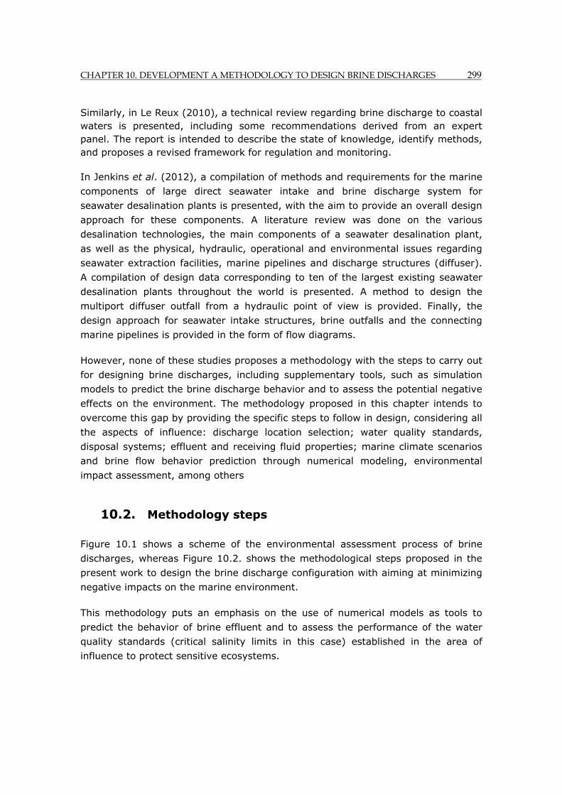
CHAPTER 10. DEVELOPMENT A METHODOLOGY TO DESIGN BRINE DISCHARGES 299
Similarly, in Le Reux (2010), a technical review regarding brine discharge to coastal waters is presented, including some recommendations derived from an expert panel. The report is intended to describe the state of knowledge, identify methods, and proposes a revised framework for regulation and monitoring.
In Jenkins et al. (2012), a compilation of methods and requirements for the marine
components of large direct seawater intake and brine discharge system for
seawater desalination plants is presented, with the aim to provide an overall design
approach for these components. A literature review was done on the various
desalination technologies, the main components of a seawater desalination plant,
as well as the physical, hydraulic, operational and environmental issues regarding
seawater extraction facilities, marine pipelines and discharge structures (diffuser).
A compilation of design data corresponding to ten of the largest existing seawater
desalination plants throughout the world is presented. A method to design the
multiport diffuser outfall from a hydraulic point of view is provided. Finally, the
design approach for seawater intake structures, brine outfalls and the connecting
marine pipelines is provided in the form of flow diagrams.
However, none of these studies proposes a methodology with the steps to carry out
for designing brine discharges, including supplementary tools, such as simulation
models to predict the brine discharge behavior and to assess the potential negative
effects on the environment. The methodology proposed in this chapter intends to
overcome this gap by providing the specific steps to follow in design, considering all
the aspects of influence: discharge location selection; water quality standards,
disposal systems; effluent and receiving fluid properties; marine climate scenarios
and brine flow behavior prediction through numerical modeling, environmental
impact assessment, among others
10.2. Methodology steps
Figure 10.1 shows a scheme of the environmental assessment process of brine
discharges, whereas Figure 10.2. shows the methodological steps proposed in the
present work to design the brine discharge configuration with aiming at minimizing
negative impacts on the marine environment.
This methodology puts an emphasis on the use of numerical models as tools to
predict the behavior of brine effluent and to assess the performance of the water
quality standards (critical salinity limits in this case) established in the area of
influence to protect sensitive ecosystems.
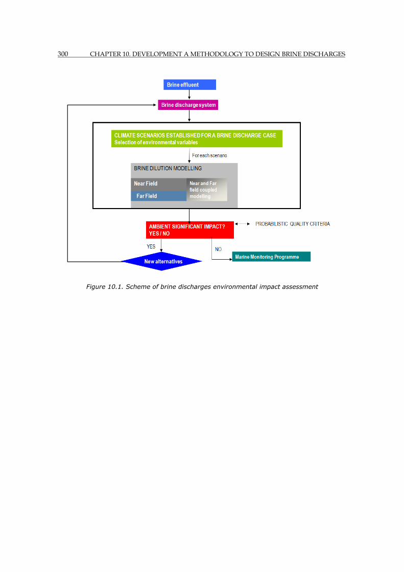
300 CHAPTER 10. DEVELOPMENT A METHODOLOGY TO DESIGN BRINE DISCHARGES
Figure 10.1. Scheme of brine discharges environmental impact assessment
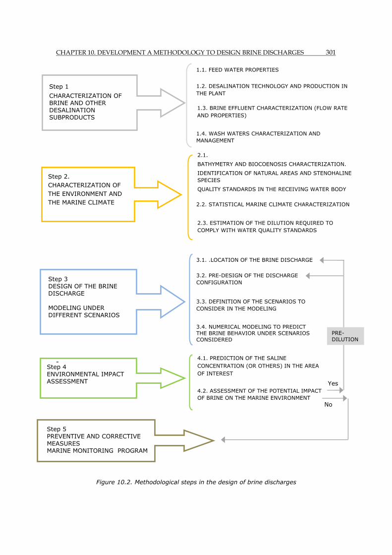
CHAPTER 10. DEVELOPMENT A METHODOLOGY TO DESIGN BRINE DISCHARGES 301
-
Figure 10.2. Methodological steps in the design of brine discharges
1.1. FEED WATER PROPERTIES
1.2. DESALINATION TECHNOLOGY AND PRODUCTION IN THE PLANT
1.4. WASH WATERS CHARACTERIZATION AND MANAGEMENT
2.1.
BATHYMETRY AND BIOCOENOSIS CHARACTERIZATION.
IDENTIFICATION OF NATURAL AREAS AND STENOHALINE SPECIES
QUALITY STANDARDS IN THE RECEIVING WATER BODY
2.3. ESTIMATION OF THE DILUTION REQUIRED TO COMPLY WITH WATER QUALITY STANDARDS
3.3. DEFINITION OF THE SCENARIOS TO CONSIDER IN THE MODELING
4.1. PREDICTION OF THE SALINE CONCENTRATION (OR OTHERS) IN THE AREA OF INTEREST
4.2. ASSESSMENT OF THE POTENTIAL IMPACT OF BRINE ON THE MARINE ENVIRONMENT
3.4. NUMERICAL MODELING TO PREDICT THE BRINE BEHAVIOR UNDER SCENARIOS CONSIDERED
Yes
PRE-DILUTION
Step 2. CHARACTERIZATION OF THE ENVIRONMENT AND THE MARINE CLIMATE
Step 3 DESIGN OF THE BRINE DISCHARGE MODELING UNDER DIFFERENT SCENARIOS
No
3.2. PRE-DESIGN OF THE DISCHARGE CONFIGURATION
2.2. STATISTICAL MARINE CLIMATE CHARACTERIZATION
1.3. BRINE EFFLUENT CHARACTERIZATION (FLOW RATE AND PROPERTIES)
3.1. .LOCATION OF THE BRINE DISCHARGE
Step 1
CHARACTERIZATION OF BRINE AND OTHER DESALINATION SUBPRODUCTS
Step 4 ENVIRONMENTAL IMPACT ASSESSMENT
Step 5 PREVENTIVE AND CORRECTIVE MEASURES MARINE MONITORING PROGRAM
302 CHAPTER 10. DEVELOPMENT A METHODOLOGY TO DESIGN BRINE DISCHARGES
10.2.1. Characterization of brine and other desalination sub-products
The desalination plant-operation regime for a representative year is defined,
considering variations in water demand. Brine discharge flow rate is calculated
applying the following formula:
1 _1
10.1
Being:
: Brine flow-rate.
_ : Feed seawater flow-rate.
: Desalinated water production.
: Conversion rate
To characterize the brine effluent, feed water properties, the type of desalination
technique and the plant´s conversion rate require to be defined previously. The
present methodology focuses on reverse osmosis desalination plants since it is
expected to be the most important technology in the future.
The quality of feed water depends on the location and type of water intake, what
determines the chemical additives and purifying processes required in the pre-
treatment. Feed water salinity, temperature and density must be in any case
defined at a representative time scale, which depends on the climate and the
marine ecosystems short and long-term brine effects.
Brine effluent properties of a SWRO plant are obtained from the feed water
properties, considering the plant conversion rate (R). Brine saline concentration ( )
is calculated from the feed seawater salinity ( _ ) by applying the formula:
_
1 10.2
For reverse osmosis desalination plants, brine pH is slightly lower than seawater
pH. Brine temperature ( ) is almost equal to seawater temperature ( _ ), or
at most 2ºC or 3 ºC higher, what has not a significant influence on the brine
behavior.
_ 10.3
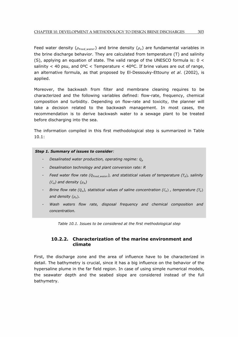
CHAPTER 10. DEVELOPMENT A METHODOLOGY TO DESIGN BRINE DISCHARGES 303
Feed water density ( _ ) and brine density ( ) are fundamental variables in
the brine discharge behavior. They are calculated from temperature (T) and salinity
(S), applying an equation of state. The valid range of the UNESCO formula is: 0 <
salinity < 40 psu, and 0ºC < Temperature < 40ºC. If brine values are out of range,
an alternative formula, as that proposed by El-Dessouky-Ettouny et al. (2002), is
applied.
Moreover, the backwash from filter and membrane cleaning requires to be
characterized and the following variables defined: flow-rate, frequency, chemical
composition and turbidity. Depending on flow-rate and toxicity, the planner will
take a decision related to the backwash management. In most cases, the
recommendation is to derive backwash water to a sewage plant to be treated
before discharging into the sea.
The information compiled in this first methodological step is summarized in Table
10.1:
Table 10.1. Issues to be considered at the first methodological step
10.2.2. Characterization of the marine environment and climate
First, the discharge zone and the area of influence have to be characterized in
detail. The bathymetry is crucial, since it has a big influence on the behavior of the
hypersaline plume in the far field region. In case of using simple numerical models,
the seawater depth and the seabed slope are considered instead of the full
bathymetry.
Step 1. Summary of issues to consider:
- Desalinated water production, operating regime:
- Desalination technology and plant conversion rate: R
- Feed water flow rate ( _ ), and statistical values of temperature ( , salinity
( ) and density ( )
- Brine flow rate ( ), statistical values of saline concentration ( , temperature (
and density ( .
- Wash waters flow rate, disposal frequency and chemical composition and
concentration.
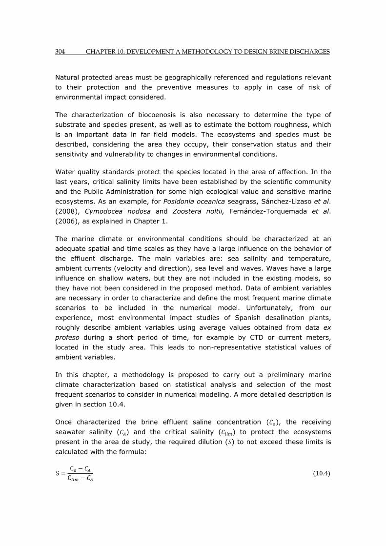
304 CHAPTER 10. DEVELOPMENT A METHODOLOGY TO DESIGN BRINE DISCHARGES
Natural protected areas must be geographically referenced and regulations relevant
to their protection and the preventive measures to apply in case of risk of
environmental impact considered.
The characterization of biocoenosis is also necessary to determine the type of
substrate and species present, as well as to estimate the bottom roughness, which
is an important data in far field models. The ecosystems and species must be
described, considering the area they occupy, their conservation status and their
sensitivity and vulnerability to changes in environmental conditions.
Water quality standards protect the species located in the area of affection. In the
last years, critical salinity limits have been established by the scientific community
and the Public Administration for some high ecological value and sensitive marine
ecosystems. As an example, for Posidonia oceanica seagrass, Sánchez-Lizaso et al.
(2008), Cymodocea nodosa and Zoostera noltii, Fernández-Torquemada et al.
(2006), as explained in Chapter 1.
The marine climate or environmental conditions should be characterized at an
adequate spatial and time scales as they have a large influence on the behavior of
the effluent discharge. The main variables are: sea salinity and temperature,
ambient currents (velocity and direction), sea level and waves. Waves have a large
influence on shallow waters, but they are not included in the existing models, so
they have not been considered in the proposed method. Data of ambient variables
are necessary in order to characterize and define the most frequent marine climate
scenarios to be included in the numerical model. Unfortunately, from our
experience, most environmental impact studies of Spanish desalination plants,
roughly describe ambient variables using average values obtained from data ex
profeso during a short period of time, for example by CTD or current meters,
located in the study area. This leads to non-representative statistical values of
ambient variables.
In this chapter, a methodology is proposed to carry out a preliminary marine
climate characterization based on statistical analysis and selection of the most
frequent scenarios to consider in numerical modeling. A more detailed description is
given in section 10.4.
Once characterized the brine effluent saline concentration ( ), the receiving
seawater salinity ( ) and the critical salinity ( ) to protect the ecosystems
present in the area de study, the required dilution ( ) to not exceed these limits is
calculated with the formula:
SCC
10.4

CHAPTER 10. DEVELOPMENT A METHODOLOGY TO DESIGN BRINE DISCHARGES 305
As previously pointed out, and must be statistical values at a time scale (day,
fortnight, month, etc.) consistent with that of the critical salinity values.
The information compiled within this second methodological step is summarized in
Table 10.2:
Table 10.2. Issues to be considered at the second methodological step
10.2.3. Design of brine discharge. Modeling and prediction of the brine behavior under different scenarios
The brine discharge location is defined considering the desalination plant site, the
presence of natural protected areas or sensitive species and the technical aspects.
It is recommended locating the discharge zone as far as possible from the area to
be protected. The bathymetric gradient and the predominant current direction are
also recommended to be taken into account, as they have a high influence on the
brine path. A high hydrodynamic environment generally increases dilution.
The most adequate discharge configuration must be selected by the planner, taking
into account the dilution rate required to comply with critical salinity values and the
particular characteristics of the receiving water body. The discharge system
determines the dilution of the effluent in the near field region, where density
differences and momentum control the geometry and mixing processes.
According to that explained in Chapter 1, the disposal system generating the
highest dilution is a submerged multiport diffuser outfall with inclined jets. In
contrast, direct surface discharge achieves low mixing and dilution, especially with
stagnant environments. Additional experimental studies are required to assess the
Step 2. Summary of issues to consider:
- Bathymetry (bottom slope and roughness) in the discharge zone and the area of
influence.
- Biocoenosis, natural protected areas and location of stenohaline species.
- Critical salinity limits ( ) and water quality standards depending on the marine
ecosystems present.
- Marine climate conditions, based on statistical analysis: temperature, salinity,
density, currents velocity and direction, all defined in an adequate time and spatial
scale.
- Dilution (S) required to perform the water quality standards.

306 CHAPTER 10. DEVELOPMENT A METHODOLOGY TO DESIGN BRINE DISCHARGES
behavior and the degree of dilution achieved in the near field region with
alternative configurations.
Once the type of discharge configuration has been decided, a pre-design is required
for carrying out a preliminary prediction of the brine behavior. Table 10.3 shows the
main parameters to define in the pre-design phase for different types of discharge
devices.
Direct surface discharge
Horizontal jet overflow spillway on
a cliff discharge
Single port submerged brine
discharge
Multiport brine discharge
Shape of the discharge channel in cross-section
Discharge channel width
Water depth at the discharge point
Port diameter
Port height above the water sea level
Port length
Jet discharge velocity
Initial discharge angle (θ)
Port diameter (d )
Port height above the sea bottom ( )
Jet discharge velocity ( )
Orientation with respect to ambient currents ( )
Those of single port and in addition:
Diffuser length ( ) and type
Diffuser orientation relative to shoreline
Horizontal angle of the jets relative to the diffuser ( )
Number of ports ( )
Port separation ( )
Table 10.3. Design parameters for different brine discharge configurations
The following criteria to maximize brine mixing and dilution are recommended to
establish the design parameter values in the pre-design of the brine discharge:
A steep slope and a small roughness bottom increase dilution in direct surface
discharges through a channel. In addition, higher divergence angles in the channel
walls, leading to turbulent eddies, increases dilution too, Jhonson et al. (1987,
1989).
For an overflow spillway in a cliff discharge: dilution increases with the jet
Densimetric Froude number, the water depth of the discharge zone and the port
height above sea level, Ruiz Mateo (2007).
For a submerged jet discharge, the criteria shown in Table 10.4 are recommended
to maximize mixing and dilution, Palomar et al. (2011).
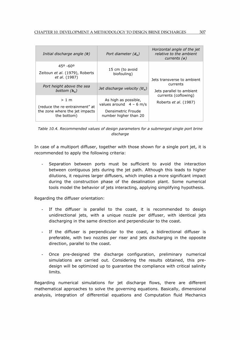
CHAPTER 10. DEVELOPMENT A METHODOLOGY TO DESIGN BRINE DISCHARGES 307
Initial discharge angle ( ) Port diameter ( ) Horizontal angle of the jet
relative to the ambient currents ( )
45º -60º
Zeitoun et al. (1979), Roberts et al. (1987)
15 cm (to avoid biofouling)
Jets transverse to ambient currents
Jets parallel to ambient currents (coflowing)
Roberts et al. (1987)
Port height above the sea bottom ( )
Jet discharge velocity ( )
> 1 m
(reduce the re-entrainment” at the zone where the jet impacts
the bottom)
As high as possible, values around 4 – 6 m/s
Densimetric Froude number higher than 20
Table 10.4. Recommended values of design parameters for a submerged single port brine discharge
In case of a multiport diffuser, together with those shown for a single port jet, it is
recommended to apply the following criteria:
- Separation between ports must be sufficient to avoid the interaction between contiguous jets during the jet path. Although this leads to higher dilutions, it requires larger diffusers, which implies a more significant impact during the construction phase of the desalination plant. Some numerical tools model the behavior of jets interacting, applying simplifying hypothesis.
Regarding the diffuser orientation:
- If the diffuser is parallel to the coast, it is recommended to design unidirectional jets, with a unique nozzle per diffuser, with identical jets discharging in the same direction and perpendicular to the coast.
- If the diffuser is perpendicular to the coast, a bidirectional diffuser is preferable, with two nozzles per riser and jets discharging in the opposite direction, parallel to the coast.
- Once pre-designed the discharge configuration, preliminary numerical simulations are carried out. Considering the results obtained, this pre- design will be optimized up to guarantee the compliance with critical salinity limits.
Regarding numerical simulations for jet discharge flows, there are different
mathematical approaches to solve the governing equations. Basically, dimensional
analysis, integration of differential equations and Computation fluid Mechanics
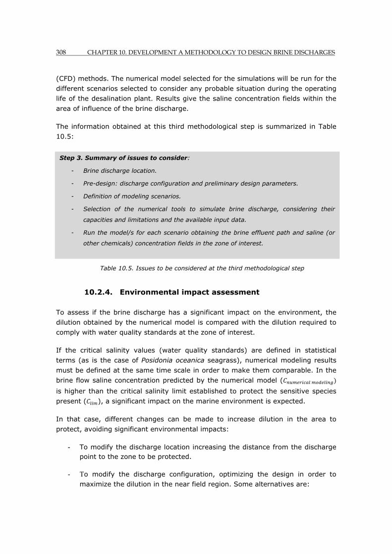
308 CHAPTER 10. DEVELOPMENT A METHODOLOGY TO DESIGN BRINE DISCHARGES
(CFD) methods. The numerical model selected for the simulations will be run for the
different scenarios selected to consider any probable situation during the operating
life of the desalination plant. Results give the saline concentration fields within the
area of influence of the brine discharge.
The information obtained at this third methodological step is summarized in Table
10.5:
Table 10.5. Issues to be considered at the third methodological step
10.2.4. Environmental impact assessment
To assess if the brine discharge has a significant impact on the environment, the
dilution obtained by the numerical model is compared with the dilution required to
comply with water quality standards at the zone of interest.
If the critical salinity values (water quality standards) are defined in statistical
terms (as is the case of Posidonia oceanica seagrass), numerical modeling results
must be defined at the same time scale in order to make them comparable. In the
brine flow saline concentration predicted by the numerical model (
is higher than the critical salinity limit established to protect the sensitive species
present ( ), a significant impact on the marine environment is expected.
In that case, different changes can be made to increase dilution in the area to
protect, avoiding significant environmental impacts:
- To modify the discharge location increasing the distance from the discharge point to the zone to be protected.
- To modify the discharge configuration, optimizing the design in order to maximize the dilution in the near field region. Some alternatives are:
Step 3. Summary of issues to consider:
- Brine discharge location.
- Pre-design: discharge configuration and preliminary design parameters.
- Definition of modeling scenarios.
- Selection of the numerical tools to simulate brine discharge, considering their
capacities and limitations and the available input data.
- Run the model/s for each scenario obtaining the brine effluent path and saline (or
other chemicals) concentration fields in the zone of interest.
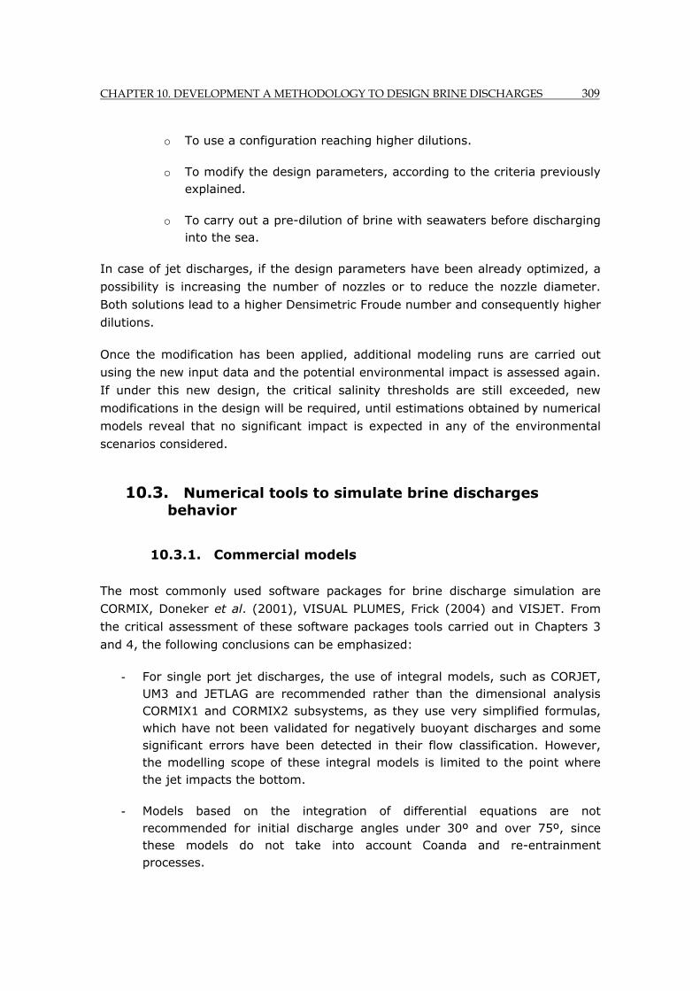
CHAPTER 10. DEVELOPMENT A METHODOLOGY TO DESIGN BRINE DISCHARGES 309
o To use a configuration reaching higher dilutions.
o To modify the design parameters, according to the criteria previously explained.
o To carry out a pre-dilution of brine with seawaters before discharging into the sea.
In case of jet discharges, if the design parameters have been already optimized, a
possibility is increasing the number of nozzles or to reduce the nozzle diameter.
Both solutions lead to a higher Densimetric Froude number and consequently higher
dilutions.
Once the modification has been applied, additional modeling runs are carried out
using the new input data and the potential environmental impact is assessed again.
If under this new design, the critical salinity thresholds are still exceeded, new
modifications in the design will be required, until estimations obtained by numerical
models reveal that no significant impact is expected in any of the environmental
scenarios considered.
10.3. Numerical tools to simulate brine discharges behavior
10.3.1. Commercial models
The most commonly used software packages for brine discharge simulation are
CORMIX, Doneker et al. (2001), VISUAL PLUMES, Frick (2004) and VISJET. From
the critical assessment of these software packages tools carried out in Chapters 3
and 4, the following conclusions can be emphasized:
- For single port jet discharges, the use of integral models, such as CORJET, UM3 and JETLAG are recommended rather than the dimensional analysis CORMIX1 and CORMIX2 subsystems, as they use very simplified formulas, which have not been validated for negatively buoyant discharges and some significant errors have been detected in their flow classification. However, the modelling scope of these integral models is limited to the point where the jet impacts the bottom.
- Models based on the integration of differential equations are not recommended for initial discharge angles under 30º and over 75º, since these models do not take into account Coanda and re-entrainment processes.
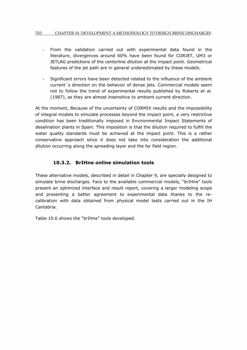
310 CHAPTER 10. DEVELOPMENT A METHODOLOGY TO DESIGN BRINE DISCHARGES
- From the validation carried out with experimental data found in the literature, divergences around 60% have been found for CORJET, UM3 or JETLAG predictions of the centerline dilution at the impact point. Geometrical features of the jet path are in general underestimated by these models.
- Significant errors have been detected related to the influence of the ambient current´s direction on the behavior of dense jets. Commercial models seem not to follow the trend of experimental results published by Roberts et al. (1987), as they are almost insensitive to ambient current direction.
At the moment, Because of the uncertainty of CORMIX results and the impossibility
of integral models to simulate processes beyond the impact point, a very restrictive
condition has been traditionally imposed in Environmental Impact Statements of
desalination plants in Spain. This imposition is that the dilution required to fulfill the
water quality standards must be achieved at the impact point. This is a rather
conservative approach since it does not take into consideration the additional
dilution occurring along the spreading layer and the far field region.
10.3.2. BrIHne online simulation tools
These alternative models, described in detail in Chapter 9, are specially designed to
simulate brine discharges. Face to the available commercial models, “brIHne” tools
present an optimized interface and result report, covering a larger modeling scope
and presenting a better agreement to experimental data thanks to the re-
calibration with data obtained from physical model tests carried out in the IH
Cantabria.
Table 10.6 shows the “brIHne” tools developed.
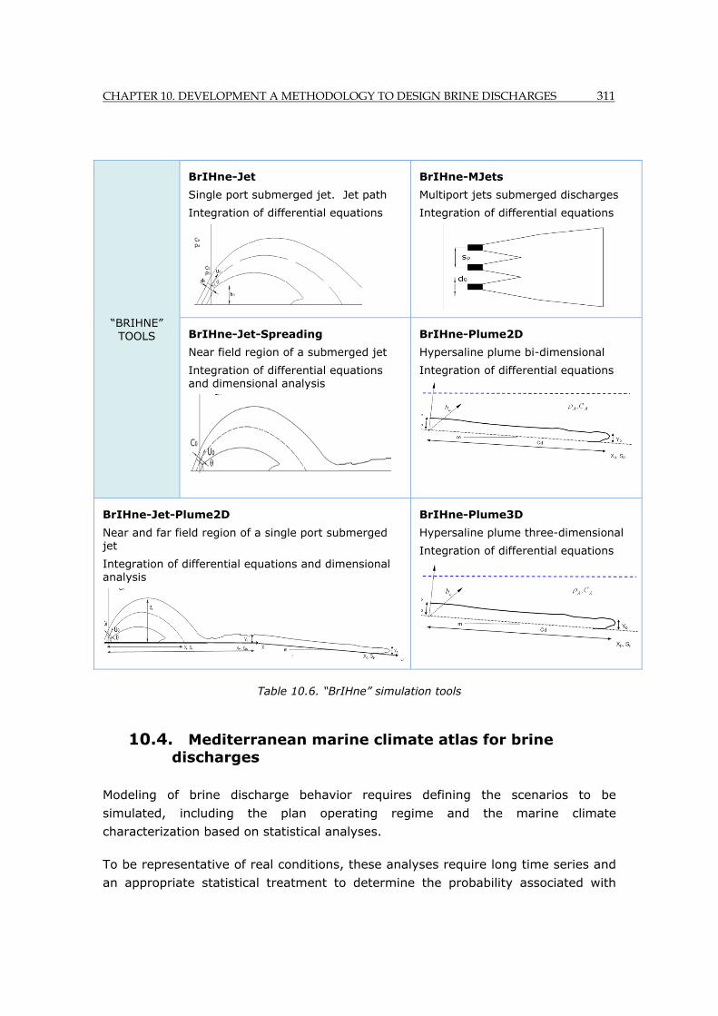
CHAPTER 10. DEVELOPMENT A METHODOLOGY TO DESIGN BRINE DISCHARGES 311
Table 10.6. “BrIHne” simulation tools
10.4. Mediterranean marine climate atlas for brine discharges
Modeling of brine discharge behavior requires defining the scenarios to be
simulated, including the plan operating regime and the marine climate
characterization based on statistical analyses.
To be representative of real conditions, these analyses require long time series and
an appropriate statistical treatment to determine the probability associated with
“BRIHNE” TOOLS
BrIHne-Jet
Single port submerged jet. Jet path
Integration of differential equations
BrIHne-MJets
Multiport jets submerged discharges
Integration of differential equations
BrIHne-Jet-Spreading
Near field region of a submerged jet
Integration of differential equations and dimensional analysis
BrIHne-Plume2D
Hypersaline plume bi-dimensional
Integration of differential equations
BrIHne-Jet-Plume2D
Near and far field region of a single port submerged jet
Integration of differential equations and dimensional analysis
BrIHne-Plume3D
Hypersaline plume three-dimensional
Integration of differential equations
312 CHAPTER 10. DEVELOPMENT A METHODOLOGY TO DESIGN BRINE DISCHARGES
each value, as well as criteria to select multidimensional scenarios to consider in
the simulation of brine discharges. The time scale of the statistical analyses must
be consistent with the climate pattern and the water quality standards established
for the protection of the existing ecosystems.
In the framework of the methodology here presented, a Marine Climate Atlas to
define the environmental scenarios for brine discharges in the Spanish
Mediterranean Sea has been developed following the next steps:
1 Identification of the variables with the highest influence on brine discharge
behavior. Ambient currents (intensity and direction), salinity, temperature, sea
level were selected Bottom slope and roughness also have a significant influence in
the far field region.
2. Identification of the ambient variables considered by the existing commercial
models. Taking into account this fact, waves have been neglected in the Atlas.
3. Definition of the area of interest. In this case, the Spanish Mediterranean region
has been divided into 35 transects representing 37 zones. Each transect has two
points at different distances from the coast (between -20 and -100 m). Each point
includes data at three different depths within the water column: sea surface, mid-
depth and sea bottom. Figure 10.3 shows the study area and the transects defined.
4. Selection of the marine climate databases with the longest time series available.
In our case, three databases were used to define sea salinity, temperature, ambient
currents and sea level variation in the area of interest.
5. When necessary, a statistical or numerical downscaling is carried out to increase
the time or spatial resolution of the study area.
6. Statistical characterization of the variables to determine the probability
associated to each value.
7. Criteria to select representative multidimensional variable scenarios. The most
frequent and less favorable scenarios are considered in the numerical modeling.
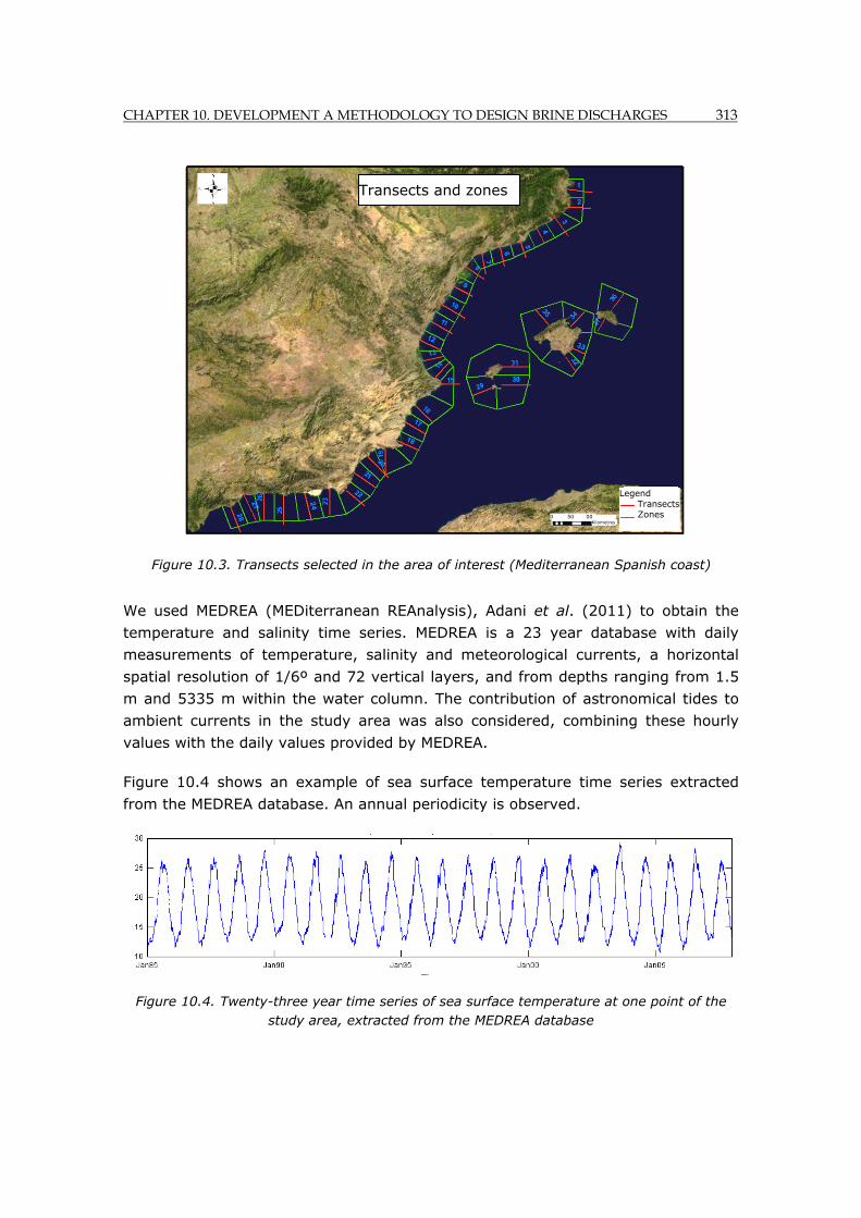
CHAPTER 10. DEVELOPMENT A METHODOLOGY TO DESIGN BRINE DISCHARGES 313
Figure 10.3. Transects selected in the area of interest (Mediterranean Spanish coast)
We used MEDREA (MEDiterranean REAnalysis), Adani et al. (2011) to obtain the
temperature and salinity time series. MEDREA is a 23 year database with daily
measurements of temperature, salinity and meteorological currents, a horizontal
spatial resolution of 1/6º and 72 vertical layers, and from depths ranging from 1.5
m and 5335 m within the water column. The contribution of astronomical tides to
ambient currents in the study area was also considered, combining these hourly
values with the daily values provided by MEDREA.
Figure 10.4 shows an example of sea surface temperature time series extracted
from the MEDREA database. An annual periodicity is observed.
Figure 10.4. Twenty-three year time series of sea surface temperature at one point of the study area, extracted from the MEDREA database
Transects and zones
Kilometres 0 50 00
Legend Transects Zones
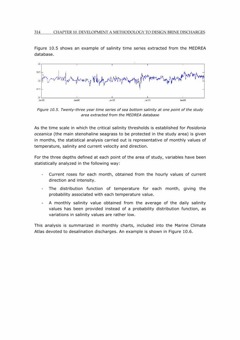
314 CHAPTER 10. DEVELOPMENT A METHODOLOGY TO DESIGN BRINE DISCHARGES
Figure 10.5 shows an example of salinity time series extracted from the MEDREA
database.
Figure 10.5. Twenty-three year time series of sea bottom salinity at one point of the study area extracted from the MEDREA database
As the time scale in which the critical salinity thresholds is established for Posidonia
oceanica (the main stenohaline seagrass to be protected in the study area) is given
in months, the statistical analysis carried out is representative of monthly values of
temperature, salinity and current velocity and direction.
For the three depths defined at each point of the area of study, variables have been
statistically analyzed in the following way:
- Current roses for each month, obtained from the hourly values of current direction and intensity.
- The distribution function of temperature for each month, giving the probability associated with each temperature value.
- A monthly salinity value obtained from the average of the daily salinity values has been provided instead of a probability distribution function, as variations in salinity values are rather low.
This analysis is summarized in monthly charts, included into the Marine Climate
Atlas devoted to desalination discharges. An example is shown in Figure 10.6.
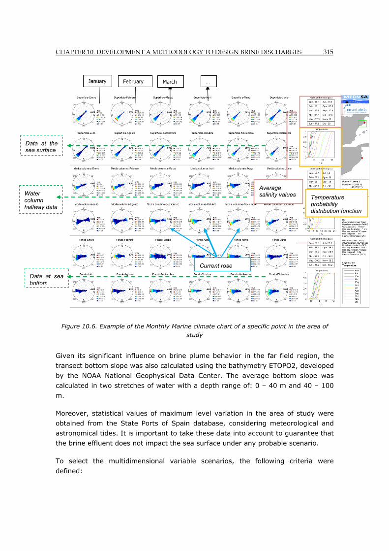
CHAPTER 10. DEVELOPMENT A METHODOLOGY TO DESIGN BRINE DISCHARGES 315
Figure 10.6. Example of the Monthly Marine climate chart of a specific point in the area of study
Given its significant influence on brine plume behavior in the far field region, the
transect bottom slope was also calculated using the bathymetry ETOPO2, developed
by the NOAA National Geophysical Data Center. The average bottom slope was
calculated in two stretches of water with a depth range of: 0 – 40 m and 40 – 100
m.
Moreover, statistical values of maximum level variation in the area of study were
obtained from the State Ports of Spain database, considering meteorological and
astronomical tides. It is important to take these data into account to guarantee that
the brine effluent does not impact the sea surface under any probable scenario.
To select the multidimensional variable scenarios, the following criteria were
defined:
January February March …
Data at the sea surface
Water column halfway data
Data at sea bottom
Temperature probability distribution function
Average salinity values
Current rose

316 CHAPTER 10. DEVELOPMENT A METHODOLOGY TO DESIGN BRINE DISCHARGES
- The salinity value to consider in any monthly scenario is the daily average value in each level of the water column.
- The temperature value to consider in any monthly scenario is the daily value corresponding to the 50 percentile (a value with a probability of 0.5 not to be exceeded) in each level of the water column under study.
- The density value is calculated from these temperature and salinity values applying an equation of state.
The current values (intensity and direction) to select for the scenarios are those
with the highest frequency and less favorable for dilution. Regarding intensities, the
less favorable currents are those with the lowest intensities, while regarding
directions, those opposite to the brine flux or those leading the brine flow to the
zone to protect are the less desired. Hence, both situations must be considered to
define the scenarios for numerical modeling.
This methodology is now being improved by applying statistical techniques of
selection (Max-Diss, Maximum Dissimilitude Algorithm) to classify the
oceanographic situations in climatic patterns. The “P” most frequent scenarios
(multidimensional variables) are determined and considered in the numerical
modeling. A statistical analysis is carried out to characterize the monthly variability
of the generated scenarios, assigning a probability to each situation.
10.5. Application of the methodology to a real case
This section shows an example of how the proposed methodology is applied to a
putative desalination plant in Spain. The plant is supposed to be located on the
province of Valencia along the Mediterranean coast, eastern of Spain. The planned
desalination plant works using reverse osmosis to desalinate seawater obtained
through an open water intake. The brine discharge must be designed to achieve a
dilution high enough to avoid negative environmental impacts on the marine
ecosystems located in the area of influence.
Following the methodological steps described before, the brine discharge is
designed in the following subsections.

CHAPTER 10. DEVELOPMENT A METHODOLOGY TO DESIGN BRINE DISCHARGES 317
10.5.1. Characterization of brine and other sub-products
Feed water characterization
The location and configuration of the plant´s water intake, as well as the required
pre-treatment method are defined taking into account technical, environmental and
economic criteria.
The seawater intake is supposed to be located at a 15 m depth, the mouth being at
7 m above the sea bottom, in order to get a high feed water quality.
Data of feed water temperature and salinity, required to characterize the brine
effluent, are obtained from the Marine Climate Atlas at the time–scale of months,
according to the critical salinity limits established for the Posidonia oceanica and
Cymodocea nodosa seagrasses. The point of the Atlas closest to the real water
intake location is selected for the characterization. Each point is characterized in the
Atlas by three depths (surface. Mid-depth and bottom). In this case, values at the
bottom are considered.
Table 10.7 shows the values of temperature, salinity and density of the sea feed
water obtained from that closest point to the water intake location. Density is
calculated applying the UNESCO equation of state.
FEED WATER
Jan. Feb. Mar. April May June July Aug. Sep. Oct. Nov. Dec.
°
13.5 12.5 14 14.5 15.5 16.5 18 19 20.5 20.5 18 15
37.6 37.7 37.7 37.7 37.7 37.8 37.7 37.6 37.6 37.5 37.6 37.6
/ ³
1028.3 1028.6 1028.3 1028.2 1028 1028 1027.3 1027 1026.6 1027.5 1027.3 1028
Table 10.7. Feed water temperature, salinity and density monthly representative values
Desalination technology
The planned desalination plant uses reverse osmosis as desalination technology,
with a conversion rate R = 45%, to separate salt from seawater.
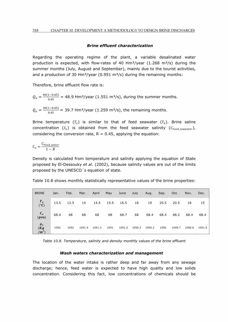
318 CHAPTER 10. DEVELOPMENT A METHODOLOGY TO DESIGN BRINE DISCHARGES
Brine effluent characterization
Regarding the operating regime of the plant, a variable desalinated water
production is expected, with flow-rates of 40 Hm³/year (1.268 m³/s) during the
summer months (July, August and September), mainly due to the tourist activities,
and a production of 30 Hm³/year (0.951 m³/s) during the remaining months:
Therefore, brine effluent flow rate is:
.
. = 48.9 Hm³/year (1.551 m³/s), during the summer months.
.
. = 39.7 Hm³/year (1.259 m³/s), the remaining months.
Brine temperature ( ) is similar to that of feed seawater ( ). Brine saline
concentration ( ) is obtained from the feed seawater salinity ( _ ),
considering the conversion rate, R = 0.45, applying the equation:
CC _
1
Density is calculated from temperature and salinity applying the equation of State
proposed by El-Dessouky et al. (2002), because salinity values are out of the limits
proposed by the UNESCO´s equation of state.
Table 10.8 shows monthly statistically representative values of the brine properties:
BRINE Jan. Feb. Mar. April May June July Aug. Sep. Oct. Nov. Dec.
°
13.5 12.5 14 14.5 15.5 16.5 18 19 20.5 20.5 18 15
68.4 68 68 68 68 68.7 68 68.4 68.4 68.2 68.4 68.4
/ ³
1052 1052 1051.4 1051.3 1051 1051.2 1050.3 1050.3 1050 1049.7 1050.6 1051.5
Table 10.8. Temperature, salinity and density monthly values of the brine effluent
Wash waters characterization and management
The location of the water intake is rather deep and far away from any sewage
discharge; hence, feed water is expected to have high quality and low solids
concentration. Considering this fact, low concentrations of chemicals should be
CHAPTER 10. DEVELOPMENT A METHODOLOGY TO DESIGN BRINE DISCHARGES 319
added during pre-treatment and no chemical pollution is expected to be present in
brine.
To avoid any risk of chemical pollution, wash waters derived from filter and
membrane cleaning will be divert to a sewage treatment plant and purified before
disposing them into the sea.
10.5.2. Characterization of the environment and the marine climate
Bathymetry and biocoenosis. Identification of natural areas and stenohaline species. Water quality standards
Bathymetry and biocoenosis studies have been carried out in the potential area of
influence of the brine. The field study reveals a sandy sea bottom, with two
Posidonia oceanica and Cymodocea nodosa meadows, covering areas of 150
hectares and 100 hectares, respectively, both in an excellent state of preservation.
The Cymodocea meadow is located 1500 m off the coast and 500 m west of the
desalination plant, at a depth of 12 m, whereas the Posidonia meadow is located
3500 m off the coast, right in front of the desalination plant, at a depth of about 20
m.
Both species are protected by European legislation since species with a high
ecological value, hence significant impacts are not allowed except for an urgent
social reason and only if there is no any other alternative to the project.
Although there is no regulation in Spain and Europe concerning brine discharges,
the following critical salinity thresholds, obtained by the scientific community, have
been recently established by Spanish environmental authorities as water quality
standards to protect these two species:
For Posidonia oceanica, Sánchez-Lizaso et al. (2008):
- Not to exceed a salinity of 38.5 psu in more than 25% of the measurements, C , 38.5 psu.
- Not to exceed a salinity of 40 psu in more than 5% of the measurements, C , 40 psu.
The time scale considered to protect this seagrass is not to exceed those limits over
a thirty days period of time (one month), criteria adopted based on the biological
research carried out with these marine plants in laboratory and ad hoc.
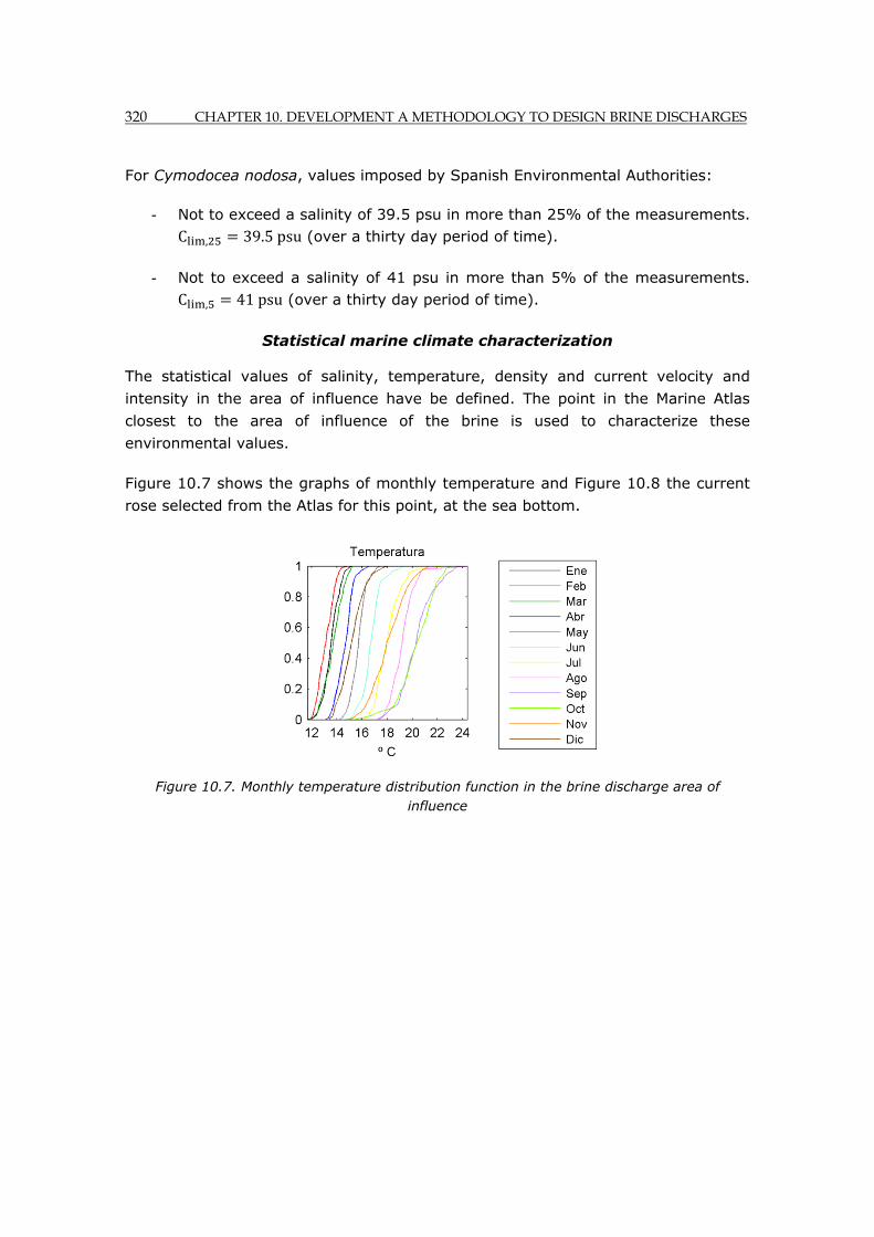
320 CHAPTER 10. DEVELOPMENT A METHODOLOGY TO DESIGN BRINE DISCHARGES
For Cymodocea nodosa, values imposed by Spanish Environmental Authorities:
- Not to exceed a salinity of 39.5 psu in more than 25% of the measurements. C , 39.5 psu (over a thirty day period of time).
- Not to exceed a salinity of 41 psu in more than 5% of the measurements. C , 41 psu (over a thirty day period of time).
Statistical marine climate characterization
The statistical values of salinity, temperature, density and current velocity and
intensity in the area of influence have be defined. The point in the Marine Atlas
closest to the area of influence of the brine is used to characterize these
environmental values.
Figure 10.7 shows the graphs of monthly temperature and Figure 10.8 the current
rose selected from the Atlas for this point, at the sea bottom.
Figure 10.7. Monthly temperature distribution function in the brine discharge area of influence
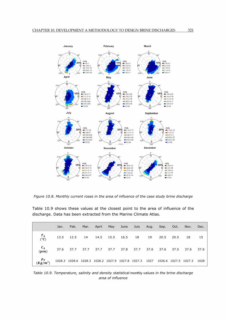
CHAPTER 10. DEVELOPMENT A METHODOLOGY TO DESIGN BRINE DISCHARGES 321
Figure 10.8. Monthly current roses in the area of influence of the case study brine discharge
Table 10.9 shows these values at the closest point to the area of influence of the
discharge. Data has been extracted from the Marine Climate Atlas.
Jan. Feb. Mar. April May June July Aug. Sep. Oct. Nov. Dec.
°
13.5 12.5 14 14.5 15.5 16.5 18 19 20.5 20.5 18 15
37.6 37.7 37.7 37.7 37.7 37.8 37.7 37.6 37.6 37.5 37.6 37.6
/ ³
1028.3 1028.6 1028.3 1028.2 1027.9 1027.8 1027.3 1027 1026.6 1027.5 1027.3 1028
Table 10.9. Temperature, salinity and density statistical monthly values in the brine discharge area of influence

322 CHAPTER 10. DEVELOPMENT A METHODOLOGY TO DESIGN BRINE DISCHARGES
The most frequent direction-velocity values of currents are selected together with
the values of the most unfavorable situations (low velocities and opposite to the
jet´s direction), and presented in Table 10.10.
PREDOMINANT CURRENT FLOW
DIRECTION
PREDOMINANT CURRENT FLOW 1
PREDOMINANT CURRENT
Direction Frequen. Direction Velocity (m/s)
Frequen. Direction Velocity (m/s)
Frequen.
January SSW 16% SSW 0.06 12% ENE 0.06 12%
February E 14% E 0.025 8% E 0.075 5%
March SSE 14% SSE 0.025 9% ESE 0.025 11%
April SSE 14% S 0.015 7% SSE 0.045 7%
May NNE 14% NNE 0.02 13%
June NNE 13% NNE 0.02 12% N 0.02 11%
July N 15% N 0.01 8% N 0.03 7%
August N 18% N 0.015 14%
Septem. N 18% N 0.01 10% N 0.04 6%
October N 18% N 0.02 10% SSW 0.02 9%
Novemb. SW 16% SW 0.035 14% SSW 0.02 13%
Decem. SW 16% SW 0.025 9.5% SSW 0.025 10%
Table 10.10. Predominant ambient currents in the discharge zone and the area of influence
According to Table 10.10, the predominant direction is variable, NNE and N
between May and October, and SW and SSE between November and April. This
information is useful to decide the jets orientation, as co-flowing and transverse
directions increase brine dilution, while opposite currents reduce dilution, Roberts et
al. (1987). If the diffuser is set parallel to the coast and the jets perpendicular to
the diffuser, the discharge would be oriented ESE (according to the maximum
bottom slope), so the SSW and NNE currents would be perpendicular to the jets
and hence, favorable to dilution.
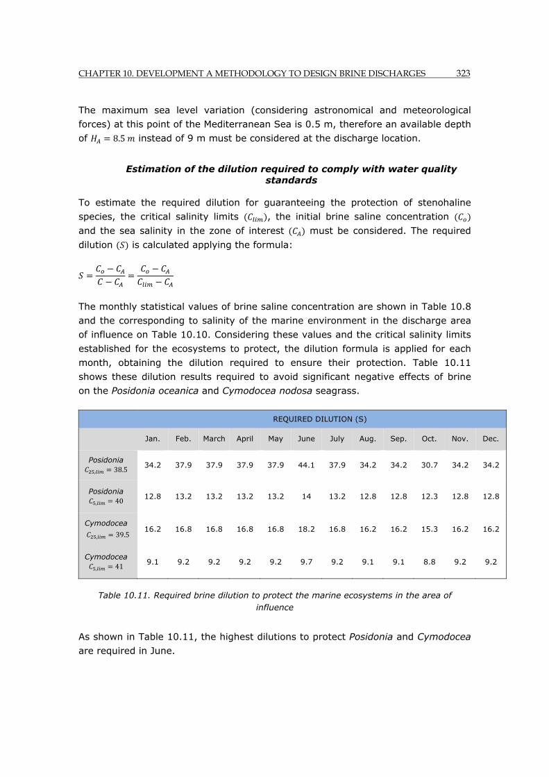
CHAPTER 10. DEVELOPMENT A METHODOLOGY TO DESIGN BRINE DISCHARGES 323
The maximum sea level variation (considering astronomical and meteorological
forces) at this point of the Mediterranean Sea is 0.5 m, therefore an available depth
of 8.5 instead of 9 m must be considered at the discharge location.
Estimation of the dilution required to comply with water quality standards
To estimate the required dilution for guaranteeing the protection of stenohaline
species, the critical salinity limits , the initial brine saline concentration
and the sea salinity in the zone of interest must be considered. The required
dilution is calculated applying the formula:
The monthly statistical values of brine saline concentration are shown in Table 10.8
and the corresponding to salinity of the marine environment in the discharge area
of influence on Table 10.10. Considering these values and the critical salinity limits
established for the ecosystems to protect, the dilution formula is applied for each
month, obtaining the dilution required to ensure their protection. Table 10.11
shows these dilution results required to avoid significant negative effects of brine
on the Posidonia oceanica and Cymodocea nodosa seagrass.
REQUIRED DILUTION (S)
Jan. Feb. March April May June July Aug. Sep. Oct. Nov. Dec.
Posidonia , 38.5 34.2 37.9 37.9 37.9 37.9 44.1 37.9 34.2 34.2 30.7 34.2 34.2
Posidonia , 40 12.8 13.2 13.2 13.2 13.2 14 13.2 12.8 12.8 12.3 12.8 12.8
Cymodocea
, 39.5 16.2 16.8 16.8 16.8 16.8 18.2 16.8 16.2 16.2 15.3 16.2 16.2
Cymodocea , 41 9.1 9.2 9.2 9.2 9.2 9.7 9.2 9.1 9.1 8.8 9.2 9.2
Table 10.11. Required brine dilution to protect the marine ecosystems in the area of influence
As shown in Table 10.11, the highest dilutions to protect Posidonia and Cymodocea
are required in June.

324 CHAPTER 10. DEVELOPMENT A METHODOLOGY TO DESIGN BRINE DISCHARGES
10.5.3. Design of the brine discharge. Modeling and prediction of the brine behavior under different scenarios
Location of the brine discharge
The dilution rate required to protect marine ecosystems (Table 8) do not make
surface direct discharge a recommendable option since this configuration achieves
very low dilutions in the near field region. A more adequate configuration is a
submerged multiport jet discharge, as it attains huge dilutions.
Regarding discharge location, the best option would be to place it east of the plant,
in front of the Cymodocea nodosa meadow, because, although the brine discharge
would be closer to a seagrass meadow, the required dilution would be lower. This
location also ensures that the Posidonia will not be affected, as it lies at the west of
the discharge and rather far away from it.
The average depth of the discharge zone must be sufficient to avoid the impact of
the jets with the sea surface. According to this, the discharge must be located as
far from the Cymodocea meadow as possible, but ensuring that the impact does not
occur under any environmental condition. As a compromise solution, we decided to
locate the discharge at a depth of 9 and at 1100 m from the coast, that is,
400 m away from the Cymodocea nodosa meadow.
Pre-design
Following the recommendations set forth in this work, the following design
parameters are proposed for the brine discharge configuration:
- Outfall perpendicular to the coast, finishing with a diffuser line at the end edge, parallel to the coast.
- Unidirectional diffuser with ports separated the same distance from each other. Identical jets with a horizontal orientation perpendicular to the diffuser, hence (in this case) ESE.
- Initial discharge angle, 60°.
- Port height: 0.5 , instead of higher than 1 m, as the water depth is limited in this case.
- Port diameter: 0.2 .
- Separation between ports ( ) sufficient to avoid interaction between jets.
CHAPTER 10. DEVELOPMENT A METHODOLOGY TO DESIGN BRINE DISCHARGES 325
- Densimetric Froude number, 20, which results, for a relative density of
∆ 23 / ³ and a port diameter 0.2 , in an initial
discharge velocity of 4.2 / .
Considering these data, the flow rate discharged by each nozzle is:
4.2.
0.131 ³/ .
The number of nozzles required in the diffuser line is calculated considering the
production flow rate and the port flow rate:
Summer months: .
.11.8 12 nozzles.
Remaining months: .
.9.61 10 nozzles.
As the adequate number of ports is different for each situation, there are two
possibilities:
- To construct the diffuser with twelve ports and to close four of them during the months of less production.
- To reduce the port diameter by a seal or some other mechanism during the months of less production, in such a way that the Densimetric Froude number in each jet is maintained.
If the previous measures are too complicated, a compromise in the number of
nozzles should be found. Considering the required dilution (Table 10.11), the most
critical month is June. Considering current velocity and direction, the summer
months are also the most critical.
In this case, we have adopted the second solution. A priori, ten ports are
considered an adequate choice. A re-calculation of values using this compromise
solution give the following results:
Summer months: .0.155 ³/ . Hence, the exit velocity is: .
/
4.9 / , and the Densimetric Froude number: .
. .23.4.
Remaining months: .0.1259 ³/ . Hence, the exit velocity is:
.
/4 / , and the Densimetric Froude number: .
. .19.1.
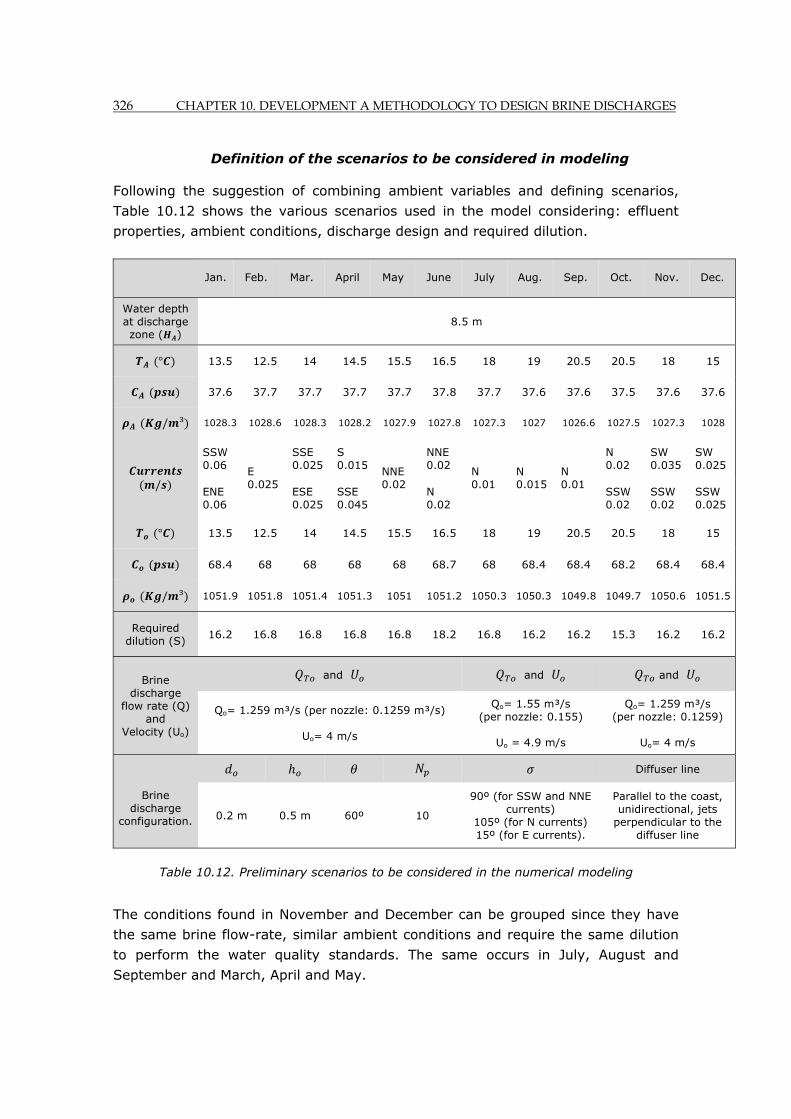
326 CHAPTER 10. DEVELOPMENT A METHODOLOGY TO DESIGN BRINE DISCHARGES
Definition of the scenarios to be considered in modeling
Following the suggestion of combining ambient variables and defining scenarios,
Table 10.12 shows the various scenarios used in the model considering: effluent
properties, ambient conditions, discharge design and required dilution.
Jan. Feb. Mar. April May June July Aug. Sep. Oct. Nov. Dec.
Water depth at discharge zone ( )
8.5 m
° 13.5 12.5 14 14.5 15.5 16.5 18 19 20.5 20.5 18 15
37.6 37.7 37.7 37.7 37.7 37.8 37.7 37.6 37.6 37.5 37.6 37.6
/ ³ 1028.3 1028.6 1028.3 1028.2 1027.9 1027.8 1027.3 1027 1026.6 1027.5 1027.3 1028
/
SSW 0.06 E
0.025
SSE 0.025
S 0.015 NNE
0.02
NNE 0.02 N
0.01 N 0.015
N 0.01
N 0.02
SW 0.035
SW 0.025
ENE 0.06
ESE 0.025
SSE 0.045
N 0.02
SSW 0.02
SSW 0.02
SSW 0.025
° 13.5 12.5 14 14.5 15.5 16.5 18 19 20.5 20.5 18 15
68.4 68 68 68 68 68.7 68 68.4 68.4 68.2 68.4 68.4
/ ³ 1051.9 1051.8 1051.4 1051.3 1051 1051.2 1050.3 1050.3 1049.8 1049.7 1050.6 1051.5
Required dilution (S)
16.2 16.8 16.8 16.8 16.8 18.2 16.8 16.2 16.2 15.3 16.2 16.2
Brine discharge
flow rate (Q) and
Velocity (Uo)
and and and
Qo= 1.259 m³/s (per nozzle: 0.1259 m³/s)
Uo= 4 m/s
Qo= 1.55 m³/s (per nozzle: 0.155)
Uo = 4.9 m/s
Qo= 1.259 m³/s (per nozzle: 0.1259)
Uo= 4 m/s
Brine
discharge configuration.
Diffuser line
0.2 m 0.5 m 60º 10
90º (for SSW and NNE currents)
105º (for N currents) 15º (for E currents).
Parallel to the coast, unidirectional, jets
perpendicular to the diffuser line
Table 10.12. Preliminary scenarios to be considered in the numerical modeling
The conditions found in November and December can be grouped since they have
the same brine flow-rate, similar ambient conditions and require the same dilution
to perform the water quality standards. The same occurs in July, August and
September and March, April and May.
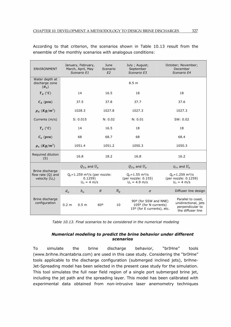
CHAPTER 10. DEVELOPMENT A METHODOLOGY TO DESIGN BRINE DISCHARGES 327
According to that criterion, the scenarios shown in Table 10.13 result from the
ensemble of the monthly scenarios with analogous conditions:
ENVIRONMENT January, February, March, April, May
Scenario E1
June Scenario
E2
July ; August; September Scenario E3
October; November; December
Scenario E4
Water depth at discharge zone
( ) 8.5 m
° 14 16.5 18 18
37.5 37.8 37.7 37.6
/ ³ 1028.3 1027.8 1027.3 1027.3
Currents (m/s) S: 0.015 N: 0.02 N: 0.01 SW: 0.02
° 14 16.5 18 18
68 68.7 68 68.4
/ ³ 1051.4 1051.2 1050.3 1050.3
Required dilution (S)
16.8 18.2 16.8 16.2
Brine discharge flow rate (Q) and
velocity (Uo)
and and and
Qo=1.259 m³/s (per nozzle: 0.1259)
Uo = 4 m/s
Qo=1.55 m³/s (per nozzle: 0.155)
Uo = 4.9 m/s
Qo=1.259 m³/s (per nozzle: 0.1259)
Uo = 4 m/s
Brine discharge configuration
Diffuser line design
0.2 m 0.5 m 60º 10 90º (for SSW and NNE) 105º (for N currents)
15º (for E currents), etc.
Parallel to coast, unidirectional, jets perpendicular to the diffuser line
Table 10.13. Final scenarios to be considered in the numerical modeling
Numerical modeling to predict the brine behavior under different scenarios
To simulate the brine discharge behavior, “brIHne” tools
(www.brihne.ihcantabria.com) are used in this case study. Considering the “brIHne”
tools applicable to the discharge configuration (submerged inclined jets), brihne-
Jet-Spreading model has been selected in the present case study for the simulation.
This tool simulates the full near field region of a single port submerged brine jet,
including the jet path and the spreading layer. This model has been calibrated with
experimental data obtained from non-intrusive laser anemometry techniques
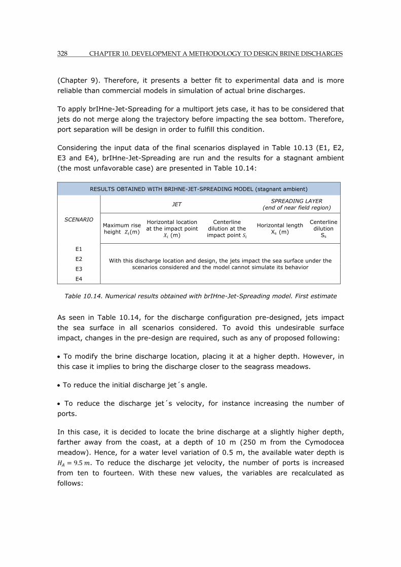
328 CHAPTER 10. DEVELOPMENT A METHODOLOGY TO DESIGN BRINE DISCHARGES
(Chapter 9). Therefore, it presents a better fit to experimental data and is more
reliable than commercial models in simulation of actual brine discharges.
To apply brIHne-Jet-Spreading for a multiport jets case, it has to be considered that
jets do not merge along the trajectory before impacting the sea bottom. Therefore,
port separation will be design in order to fulfill this condition.
Considering the input data of the final scenarios displayed in Table 10.13 (E1, E2,
E3 and E4), brIHne-Jet-Spreading are run and the results for a stagnant ambient
(the most unfavorable case) are presented in Table 10.14:
RESULTS OBTAINED WITH BRIHNE-JET-SPREADING MODEL (stagnant ambient)
SCENARIO
JET SPREADING LAYER
(end of near field region)
Maximum rise height (m)
Horizontal location at the impact point
(m)
Centerline dilution at the impact point
Horizontal length Xs (m)
Centerline dilution
Ss
E1
With this discharge location and design, the jets impact the sea surface under the scenarios considered and the model cannot simulate its behavior
E2
E3
E4
Table 10.14. Numerical results obtained with brIHne-Jet-Spreading model. First estimate
As seen in Table 10.14, for the discharge configuration pre-designed, jets impact
the sea surface in all scenarios considered. To avoid this undesirable surface
impact, changes in the pre-design are required, such as any of proposed following:
To modify the brine discharge location, placing it at a higher depth. However, in
this case it implies to bring the discharge closer to the seagrass meadows.
To reduce the initial discharge jet´s angle.
To reduce the discharge jet´s velocity, for instance increasing the number of
ports.
In this case, it is decided to locate the brine discharge at a slightly higher depth,
farther away from the coast, at a depth of 10 m (250 m from the Cymodocea
meadow). Hence, for a water level variation of 0.5 m, the available water depth is
9.5 . To reduce the discharge jet velocity, the number of ports is increased
from ten to fourteen. With these new values, the variables are recalculated as
follows:
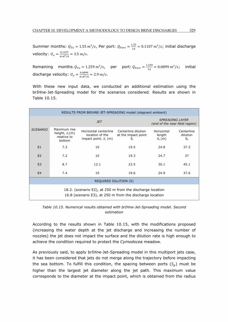
CHAPTER 10. DEVELOPMENT A METHODOLOGY TO DESIGN BRINE DISCHARGES 329
Summer months: 1.55 ³/ , Per port: .0.1107 ³/ ; initial discharge
velocity: .
/3.5 / .
Remaining months: 1.259 ³/ , per port: .0.0899 ³/ ; initial
discharge velocity: .
/2.9 / .
With these new input data, we conducted an additional estimation using the
brIHne-Jet-Spreading model for the scenarios considered. Results are shown in
Table 10.15.
Table 10.15. Numerical results obtained with brIHne-Jet-Spreading model. Second estimation
According to the results shown in Table 10.15, with the modifications proposed
(increasing the water depth at the jet discharge and increasing the number of
nozzles) the jet does not impact the surface and the dilution rate is high enough to
achieve the condition required to protect the Cymodocea meadow.
As previously said, to apply brIHne-Jet-Spreading model in this multiport jets case,
it has been considered that jets do not merge along the trajectory before impacting
the sea bottom. To fulfill this condition, the spacing between ports ( ) must be
higher than the largest jet diameter along the jet path. This maximum value
corresponds to the diameter at the impact point, which is obtained from the radius
RESULTS FROM BRIHNE-JET-SPREADING model (stagnant ambient)
SCENARIO
JET SPREADING LAYER
(end of the near field region)
Maximum rise height, (m)
relative to bottom
Horizontal centerline location of the
impact point, (m)
Centerline dilution at the impact point
Si
Horizontal length Xs (m)
Centerline dilution
Ss
E1 7.3 10 19.5 24.8 37.3
E2 7.2 10 19.3 24.7 37
E3 8.7 12.1 23.5 30.1 45.1
E4 7.4 10 19.6 24.9 37.6
REQUIRED DILUTION (S)
18.2. (scenario E2), at 250 m from the discharge location
16.8 (scenario E3), at 250 m from the discharge location
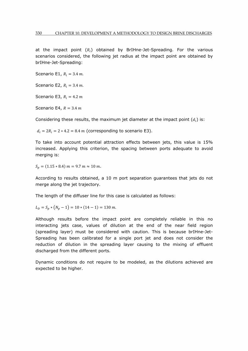
330 CHAPTER 10. DEVELOPMENT A METHODOLOGY TO DESIGN BRINE DISCHARGES
at the impact point ( ) obtained by BrIHne-Jet-Spreading. For the various
scenarios considered, the following jet radius at the impact point are obtained by
brIHne-Jet-Spreading:
Scenario E1, 3.4 .
Scenario E2, 3.4 .
Scenario E3, 4.2
Scenario E4, 3.4
Considering these results, the maximum jet diameter at the impact point ( ) is:
2 2 4.2 8.4 (corresponding to scenario E3).
To take into account potential attraction effects between jets, this value is 15%
increased. Applying this criterion, the spacing between ports adequate to avoid
merging is:
1.15 8.4 9.7 10 .
According to results obtained, a 10 m port separation guarantees that jets do not
merge along the jet trajectory.
The length of the diffuser line for this case is calculated as follows:
1 10 14 1 130 .
Although results before the impact point are completely reliable in this no
interacting jets case, values of dilution at the end of the near field region
(spreading layer) must be considered with caution. This is because brIHne-Jet-
Spreading has been calibrated for a single port jet and does not consider the
reduction of dilution in the spreading layer causing to the mixing of effluent
discharged from the different ports.
Dynamic conditions do not require to be modeled, as the dilutions achieved are
expected to be higher.
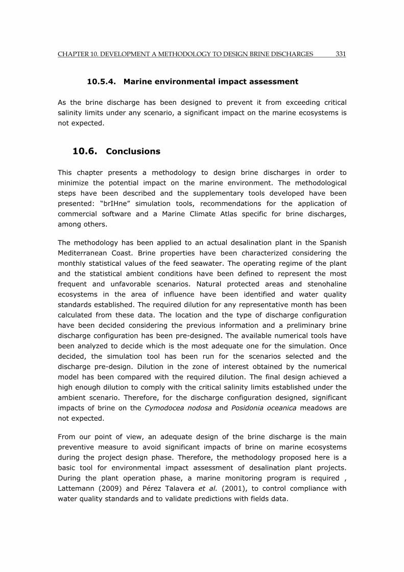
CHAPTER 10. DEVELOPMENT A METHODOLOGY TO DESIGN BRINE DISCHARGES 331
10.5.4. Marine environmental impact assessment
As the brine discharge has been designed to prevent it from exceeding critical
salinity limits under any scenario, a significant impact on the marine ecosystems is
not expected.
10.6. Conclusions
This chapter presents a methodology to design brine discharges in order to
minimize the potential impact on the marine environment. The methodological
steps have been described and the supplementary tools developed have been
presented: “brIHne” simulation tools, recommendations for the application of
commercial software and a Marine Climate Atlas specific for brine discharges,
among others.
The methodology has been applied to an actual desalination plant in the Spanish
Mediterranean Coast. Brine properties have been characterized considering the
monthly statistical values of the feed seawater. The operating regime of the plant
and the statistical ambient conditions have been defined to represent the most
frequent and unfavorable scenarios. Natural protected areas and stenohaline
ecosystems in the area of influence have been identified and water quality
standards established. The required dilution for any representative month has been
calculated from these data. The location and the type of discharge configuration
have been decided considering the previous information and a preliminary brine
discharge configuration has been pre-designed. The available numerical tools have
been analyzed to decide which is the most adequate one for the simulation. Once
decided, the simulation tool has been run for the scenarios selected and the
discharge pre-design. Dilution in the zone of interest obtained by the numerical
model has been compared with the required dilution. The final design achieved a
high enough dilution to comply with the critical salinity limits established under the
ambient scenario. Therefore, for the discharge configuration designed, significant
impacts of brine on the Cymodocea nodosa and Posidonia oceanica meadows are
not expected.
From our point of view, an adequate design of the brine discharge is the main
preventive measure to avoid significant impacts of brine on marine ecosystems
during the project design phase. Therefore, the methodology proposed here is a
basic tool for environmental impact assessment of desalination plant projects.
During the plant operation phase, a marine monitoring program is required ,
Lattemann (2009) and Pérez Talavera et al. (2001), to control compliance with
water quality standards and to validate predictions with fields data.

332 CHAPTER 10. DEVELOPMENT A METHODOLOGY TO DESIGN BRINE DISCHARGES
To make the methodology proposed in this manuscript useful to developers and
environmental authorities, the methodological guidelines and the complementary
tools have been made available through a web site (www.medvsa.es).

CHAPTER 11. CONCLUSIONS AND FUTURE RESEARCH 333
Chapter 11. CONCLUSIONS AND FUTURE RESEARCH
Chapter 11 CONCLUSIONS AND FUTURE RESEARCH
11.1 Conclusions
The increasing desalinated water production in our country (and worldwide) implies
a rising of the volume of brine effluent discharged into the sea. The evidence of
negative effects of brine on the marine ecosystems, together with the lack of
regulation in force, causes a crescent environmental concern. This concern is
aggravated by the gaps of knowledge, criteria and methodologies regarding brine
discharges.
Faced with this situation, the present Thesis was born with the overarching goal of
developing a methodology to design brine discharge minimizing the potential
impact on the marine environment. This methodology has to consider many
aspects, such as water quality standards, protected ecosystems, desalination
processes, marine climate, modeling scenarios, discharge configuration and
behavior prediction, among others.
A previous review of the State of the Art in all these aspects, summarized in
Chapter 1, has allowed identifying the main shortcomings related to brine
discharges and their effects on the marine ecosystem. Four of these scientific
shortcomings have been selected for a further research in this work, constituting
four partial objectives, which have been developed in the self-contained chapters of
this Thesis.
The first partial goal deals with the uncertainties associated to the use of the
existing commercial models to simulate brine discharges that are fundamental
predictive tools in Environmental Impact Studies. In this Thesis, these models have
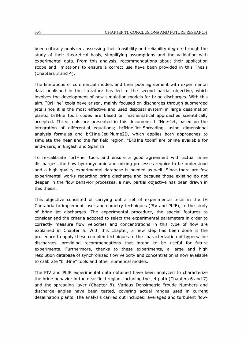
334 CHAPTER 11. CONCLUSIONS AND FUTURE RESEARCH
been critically analyzed, assessing their feasibility and reliability degree through the
study of their theoretical basis, simplifying assumptions and the validation with
experimental data. From this analysis, recommendations about their application
scope and limitations to ensure a correct use have been provided in this Thesis
(Chapters 3 and 4).
The limitations of commercial models and their poor agreement with experimental
data published in the literature has led to the second partial objective, which
involves the development of new simulation models for brine discharges. With this
aim, “BrIHne” tools have arisen, mainly focused on discharges through submerged
jets since it is the most effective and used disposal system in large desalination
plants. brIHne tools codes are based on mathematical approaches scientifically
accepted. Three tools are presented in this document: brIHne-Jet, based on the
integration of differential equations; brIHne-Jet-Spreading, using dimensional
analysis formulas and brIHne-Jet-Plume2D, which applies both approaches to
simulate the near and the far field region. “BrIHne tools” are online available for
end-users, in English and Spanish.
To re-calibrate “brIHne” tools and ensure a good agreement with actual brine
discharges, the flow hydrodynamic and mixing processes require to be understood
and a high quality experimental database is needed as well. Since there are few
experimental works regarding brine discharge and because those existing do not
deepen in the flow behavior processes, a new partial objective has been drawn in
this thesis.
This objective consisted of carrying out a set of experimental tests in the IH
Cantabria to implement laser anemometry techniques (PIV and PLIF), to the study
of brine jet discharges. The experimental procedure, the special features to
consider and the criteria adopted to select the experimental parameters in order to
correctly measure flow velocities and concentrations in this type of flow are
explained in Chapter 5. With this chapter, a new step has been done in the
procedure to apply these complex techniques to the characterization of hypersaline
discharges, providing recommendations that intend to be useful for future
experiments. Furthermore, thanks to these experiments, a large and high
resolution database of synchronized flow velocity and concentration is now available
to calibrate “brIHne” tools and other numerical models.
The PIV and PLIF experimental data obtained have been analyzed to characterize
the brine behavior in the near field region, including the jet path (Chapters 6 and 7)
and the spreading layer (Chapter 8). Various Densimetric Froude Numbers and
discharge angles have been tested, covering actual ranges used in current
desalination plants. The analysis carried out includes: averaged and turbulent flow-

CHAPTER 11. CONCLUSIONS AND FUTURE RESEARCH 335
fields, cross-sections, longitudinal profiles, calibration of dimensional analysis
formulas and the assessment of simplifying hypothesis generally assumed by
numerical models. With this analysis, particular features of negatively buoyant
inclined jets, which difficult the numerical modeling modeling and making
commercial models do not simulate this type of flow properly, have been identified.
The research carried out has allowed understanding complex processes that make
this type of flow behavior to diverge from that typical a pure jet.
The experimental database generated has been used to re-calibrate the “brIHne”
tools, Chapter 9, which provides a more accurate brine discharge prediction than
commercial models, with a better agreement to experimental data found in the
literature.
The critical assessment and validation of commercial models, the further knowledge
of brine flow behavior and the “brIHne” tools developed have been integrated in a
Methodological Guide, described in Chapter 10. The guide includes the following
steps to design brine discharges: 1) Brine and other sub-products characterization;
2) Marine environment characterization; 3) Discharge design and brine behavior
prediction; 4) Environmental Impact assessment; 5) Correction measures and
Marine Monitoring Program. The guidelines have been focused on brine from
Reverse osmosis desalination plants discharged into the Mediterranean Sea, but can
be adapted to any other desalinating region.
In summary, to achieve the technical objective of developing a methodology
guideline for brine discharges, the present work has deepened in basic scientific
research to overcome some of the knowledge gaps identified in the review of the
State of the Art. The reliability of existing simulation tools assessed, the
characterization of brine effluent behavior, the development of alternative
numerical models and the methodological guidelines provided have gone further
than the current State of the Art. Therefore, the methodology proposed includes
knowledge on the State of the Art for some issues to consider and knowledge that
goes beyond the State of the Art in the specific aspects covered in this Thesis.
336 CHAPTER 11. CONCLUSIONS AND FUTURE RESEARCH
11.2 Future Research
Considering the multiple aspects to consider in the design of brine discharges from
an environmental point of view, future research must cover diverse knowledge
fields.
Following, the main aspects requiring further investigation are summarized.
Considering the effects of brine on the marine environment, critical salinity limits
must be established, preferably in statistical terms, for benthic species with a high
ecological value existing in marine areas where brine is frequently disposed. The
potential synergistic effects of different effluent discharges, such as the mix
between brine and sewage, requires to be studied.
The marine climate characterization methodology needs to be improved, integrating
classification (Self-organizing maps) and selection algorithms (Max-Diss) to carry
out a statistical characterization of the most frequent scenarios to consider in an
adequate scale in brine discharges.
Regarding experimental research, additional discharge configuration and processes
need to be experimentally characterized with PIV and LIF non-intrusive techniques,
to deepen in its behavior, while generating a database to calibrate and validate
numerical models. In particular:
- Characterization of direct surface discharges on sand, gravel or slab beaches.
- Characterization of discharges on the mouth of channels flowing to seawaters.
- Characterization of discharges through emerging jets at various heights from seawaters.
- Characterization of discharges by multiport submerged jets, with jets merging along the jet path.
- Characterization of the hypersaline plume typical of the far field region, considering the bathymetry and roughness influence on the flow behavior
- Characterization of the influence of a dynamic environment (ambient currents and waves) on the brine behavior, for different disposal configurations and considering the near and the far field region.
CHAPTER 11. CONCLUSIONS AND FUTURE RESEARCH 337
Regarding numerical modeling, further investigation is required at different levels:
- To deepen in the governing equations of negatively buoyant jets, quantitatively evaluating the weight of each term in the flux behavior.
- To consider dimensional analysis to brine discharged different from submerged jets, in order to identify the variables with the highest influence on the flux behavior. To calibrate the semi-empirical formulas obtained with new experimental.
- Regarding models based on the integration of differential equations to simulate submerged negatively buoyant inclined jet discharges:
o To re-calibrate them, modifying their equations in order to simulate the particular features of inclined dense jets, such as the extra-spreading of the jet lower boundary.
o To analyze and validate the entrainment formulas used in these models, which cannot correctly simulate the mixing process within this type of flow.
o To analyze the hypotheses generally assumed to simulate the merging between jets, such as the assumption of an equivalent slot diffuser. To re-calibrate these assumptions to get a better fit to experimental data.
- To develop additional “brIHne” simulation tools, based on simple mathematical approaches if possible, for different discharge configurations. To re-calibrate them with high quality experimental data to guarantee accurate predictions.
- To implement advances CFD models to simulate the near field region of brine discharges under different disposal solutions.
- To implement hydrodynamic models to simulate the hypersaline plume, characteristic of the brine behavior in the far field region, considering the influence on the marine climate variables.
- To establish coupling conditions between the near and the far field region for this type of flow under different discharge configurations.

338 CHAPTER 11. CONCLUSIONS AND FUTURE RESEARCH
REFERENCES 339
REFERENCES
REFERENCES
A
Abrahamsson, H., Johansson, B., Löfdahl, L. (1994). “A turbulent plane two-
dimensional wall jet in a quiescent surrounding”, European Journal of Mechanics B.
Fluids, vol. 13, pp. 533 - 556.
Adani, M., Dobricic, S., Pinardi, N. (2011). “Qualilty assessment of a 1985-2007
Mediterranean Sea reanalisys”. Journal of Atmospheric and Ocean Technology, vol.
28, pp. 569–589.
Afgan, N. H., Al Gobaisi, D., Carvalho, M. G., Cumo, M. (1998). “Sustainable energy
management”. Renewable and sustainable energy review, vol. 2, pp. 235 – 286.
Akar, P. J., Jirka, G. H. (1991). “CORMIX2: An expert system for hydrodynamic
mixing zone analysis of conventional and toxic submerged multiport diffuser
discharges”. U.S. Environmental Protection Agency (EPA), Office of Research and
Development.
Alavian, V. (1986). “Behavior of density current on an incline”. Journal of Hydraulic
Engineering, vol. 112, No 1, pp. 27 - 42.
Ansong, J. K., Kyba, P. J., Sutherland, B. R. (2008). “Fountains impinging on a
density interface”. Journal of Fluid Mechanics, vol. 595, pp. 115 -139.
Antequera, M., Jáuregui, A. (2001). “Ensayos del comportamiento de vertidos
salinos al mar”. II Congreso Nacional de Desalación. Alicante. Asociación Española
de Desalación y Reutilización Alicante.
Arcoumanis, C., McGuirk, J. J., Palma, J. M. (1990).“On the use of fluorescent dyes
for concentration measurements in water flows”. Experiments in Fluids, vol. 10, pp.
177-180.
Ashida, K. and Egashira, G. (1977). "Basic study on turbidity currents".
Proceedings, Japan Society of Civil Engineering, No. 237, pp. 37 – 50.
340 REFERENCES
B
Billy, F. (2005). “Analyse de l’effet des surfaces texturées ans un film mince.
Application aux joints d’étanchéités”. Thèse de Doctorat, Université de Poitiers,
Poitiers, France.
Bleninguer, T. (2006). “Coupled 3D hydrodynamic models for submarine outfalls:
environmental hydraulic design and control of multiport diffusers”. Doctoral Thesis,
Institute for Hydromecanics, University Karlsruhe.
Bloomfield, L. J., Kerr, R. C. (2002). “Inclined turbulent fountains”. Journal of Fluid
Mechanics, Cambridge University Press, vol. 451, pp. 283 - 294.
Bonfligio, A., Cipollina, A., Grisaf, F., Micale, G., Brucato, G. (2008). “A
computational modelling of flow and turbulent in submerged dense jets”. Paper
presented at ICheap7.
Britter, R. E. (1979). “The spread of a negatively buoyant plume in a calm
environment”. Atmospheric Environment, vol. 13, pp. 1241 - 1247.
Britter, R. E., Simpson, J. E. (1981). “A note on the structure of the head of an
intrusive gravity current”. Journal of Fluid Mechanics, vol. 112, pp. 459 - 466.
C
Chester, R. H. (1975). Biological impact of a large-scale desalination plant at Key
West, Florida. Oceanography Series, vol. 12, pp. 99 - 153.
Cheung, S. K. B., Leung, D. Y. L., Wang, W., Lee, J. H. W., Cheung, V. (
2000).”VISJET – A computer ocean outfall modelling system”. Proceeding CGI '00.
Proceedings of the International Conference on Computer Graphics, IEEE Computer
Society Washington, DC, USA.
Christodoulou, G. C. (2001). “Lateral growth of 3-D density currents”. Proceedings
XXIX IAHR Congress, Beijing, China, Sept. 16-21, pp. 29 - 34.
Chu, V. H. (1975). “Turbulent dense plumes in a laminar cross flow”. Journal of
Hydraulic Research, vol. 13, pp. 253 - 279.
Cipollina, A., Brucato, A., Grisafi, F., Nicosia, S.(2005). “Bench-Scale investigation
of inclined dense jets”. Journal of Hydraulic Engineering, vol. 131, no 11, pp. 1017
- 1022.
REFERENCES 341
Cipollina, A., Brucato, A., Micale, G. (2009). “A mathematical tool for describing the
behavior of a dense effluent discharge”. Desalination and Water Treatment, vol. 2,
pp. 295 - 309.
Cowen, E. A.,Chang, K. A., Liao, Q. (2001). “A single-camera coupled PTV-LIF
technique”. Experiments in Fluids, vol. 31, pp. 63 - 73.
Crimaldi, J. P. (2008). “Planar laser induced fluorescence in aqueous flows”.
Experiments in Fluids, vol. 44, pp. 851 - 863.
D
Dallimore, C. J., Imberger, J., Ishikawa, T. (2001). “Entrainment and turbulence in
Saline underflow in lake Ogawara”. Journal of Hydraulic Engineering, Vol. 219, No
11, pp. 937 - 948.
David, L. (2005). “Rapport de synthèse. Habilitation à Diriger des Recherches”.
Université de Poitiers, Poitiers, France.
DBK, S.A. (Databank SpA). Special Report: “Desalination Companies”.
(www.dbk.es).
DesalData 2010/IDA. Disponible en: http://www.desaldata.com/
Doneker, R. L., Jirka, G. H. (1990). “Expert system for hydrodynamic mixing zone
analysis of conventional and toxic submerged single port discharges (CORMIX1)”.
Technical Report EPA 600-3-90-012. U.S. Environmental Protection Agency (EPA).
Doneker, R. L., Jirka, G. H. (1998) "D-CORMIX: a decision support system for hydrodynamic mixing zone analysis of continuous dredge disposal sediment plumes". Proc. Of the 25th Annual Conference on Water Resources Planning and Management, ASCE.
Doneker, R. L., Jirka, G. H. (2001). “CORMIX-GI systems for mixing zone analysis
of brine wastewater disposal”. Desalination, vol. 139, pp. 263 – 274.
Einav, R., Lokiec, F. (2003). “Environmental aspects of a desalination plant in
Ashkelon”. Desalination, vol. 156, pp. 79 - 85.
El-Dessouky, H. M, Ettouny, H. T. (2002) “Fundamentals of salt water desalination”,
(Appendix A: Thermodynamic Properties), Elsevier Science.
Ellison, T. H., Turner, J. S. (1959). “Turbulent entrainment in stratified flows”.
Journal of Fluid Mechanics, Vol. 6, pp. 423 - 448.
342 REFERENCES
Eriksson, J., Karlsson, R., Persson, J. (1998). “An experimental study of a two-
dimensional plane turbulent wall jet”. Experiments in Fluids, vol. 25, pp. 50 - 60.
Estrela, T., Vargas, E., Sánchez, J.M., Torres, M., Fariñas, M., Ruiz-Mateo, A.,
Martínez, F., Troyano, F., Paniagua, I., Medina, J.A. (2008). Libro “La desalación en
España”, editado por ACUAMED (Aguas para las Cuencas Mediterráneas) y
Ministerio de Medio Ambiente, Medio Rural y Marino.
F
Fernández-Torquemada, Y., Sánchez-Lizaso, J. L. (2005). “Effects of salinity on leak
growth and survival of the Mediterranean seagrass Posidonia Oceanica Delile”.
Journal of experimental marine biology and Ecology, vol. 320. pp 57 - 63.
Fernández Torquemada, Y., Sánchez Lizaso, J. L. (2006). “Effects of salinity on
growth and survival of Cymodocea nodosa (Ucria) Aschernon and Zostera noltii
Hornemann”. Biology Marine Mediterranean, vol. 13 (4), pp. 46 - 47.
Ferrari, S., Querzoli, G. (2006). “An experimental investigation of interaction
between dense sea discharges and wave motion”. MWWD 2006, 4th International
Conference on Marine Waste Water Disposal and Marine Environment.
Ferrari, S., Querzoli, G. (2004). “Sea discharge of brine from desalination plants: a
laboratory model of negatively buoyant jets”. MWWD 2004, 3th International
Conference on Marine Waste Water Disposal and Marine Environment.
Ferrier, A. J., Funk, D. R., Robert, P. J. W. (1993). “Application of optical techniques
to the study of plumes in stratified fluids”. Dynamics of Atmospheres and Oceans,
vol. 20, pp. 155 - 183.
Fischer, H. B., List, E. J., Imberger, J., Brooks, N. H. (1979). “Mixing in island and
coastal waters”. Academic Press, N.Y.
Frick, W. E. (2004). “Visual Plumes mixing zone modeling software”. Environmental
& Modeling Software, vol. 19, pp. 645 - 654.
Fukushima, Y., Parker, G., Pantin, H. M. (1985). “Prediction of ignitive turbidity
currents in Scripps Submarine Canyon”. Marine Geology, vol. 67, pp. 55 - 81.
G
Gacia, E., Invers, O., Ballesteros, E., Manzanera, M., Romero, R. L. (2007). “The
impact of the brine from a desalination plant on a shallow seagrass (Posidonia
REFERENCES 343
oceanica) meadow”. Estuarine, Coastal and Shelf Science, vol. 72, Issue 4, pp. 579
- 590.
Ghasemi, J., Niazi, A., Kubista, M. (2005). “Thermodynamics study of the
dimerization equilibria of rhodamine B and 6G in different ionic strengths by
photometric titration and chemometrics method”. Spectrochimica Acta, Part A. Vol.
62, pp. 649 – 656.
García, M. (1985). “Experimental study of turbidity currents”. Tesis de Maestría en
Ingeniería Civil. Universidad de Minnesota, Minneapolis.
García, M. H. (1996). “Environmental hydrodynamics”. Sante Fe, Argentina:
Publications Center, Universidad Nacional del Litoral.
Gaskin, S. J. (1995).“Single buoyant jet in a cross flow and the advected line
thermal”. Ph.D Thesis, University of Canterbury, Christchurch,New Zealand.
George, W. K., Abrahamsson, H., Eriksson, J., Karlsson, R. I., Lofdahl, L., Wosnik,
M. (2000). “A similarity theory for the turbulent plane wall jet”. Journal of Fluid
Mechanics, Vol. 425, pp. 368 - 411.
Gomeshi. (1995). “Reservoir sedimentation modelling”. Research online, University
of Wollongong, Thesis collection.
Gungor, E., Roberts, P. J. W. (2009). “Experimental studies on vertical dense jets in
a Flowing Current”. Journal of Hydraulic Engineering, vol. 135, Nº. 11, pp. 935 -
948.
H
Haghiabi, A. H. (2004). "The study of bed slope effect on velocity and concentration
profiles of density currents". Ph.D. Thesis, Shahid Chamran University, Ahwaz, Iran.
Hartmanna, T., Paviet-Hartmanna, P., Wettelandb, C., Ningping Luc. (2005).
“Spectroscopic determination of hypochlorous acid,in chloride brine solutions,
featuring 5MeV proton beam line experiments”. Radiation Physics and Chemistry,
vol. 66, pp. 335–341.
Hebbert, B., Imberger, J., Loh, I., Patterson, J. (1979). “Collie River Underflow into
the Wellington Reservoir”. Journal of Hydraulic Division., vol. 105 (5), pp. 533 –
545.
344 REFERENCES
Hodges, B. R. (2006). “Fate of desalination brine in Texas coastal bays and
estuaries. Advanced technology program”. Department of Civil Engineering,
University of Texas at Austin.
Hoepner, T. (1999). “A procedure for environmental impact assessment (EIA) for
seawater desalination plants”. Desalination, vol. 124, pp. 1 – 12.
Houcine, I., Vivier, H., Plasari, E., Villermaux, J. (1996). “Planar laser induced
fluorescence technique for measurements of concentration fields in continuous
stirred tank reactors”. Experiments in Fluids, vol. 22, pp. 95 – 102.
I
Instituto Tecnológico de Canarias. S.A. “Venturi project” , funded by the National
Program for Experimental Development of the Spanish Ministry of the Environment
and Rural and Marine Affairs (2008 - 2010).
J
Jenkins, S., Paduan, J., Roberts, P. J. W., Schlenk, D., Weis, J. (2012).
“Management of brine discharges to coastal waters. Recommendations of a Science
Advisory Panel”. Technical Report 694, submitted as a request of the California
Water Resources Control Board.
Jhonson, T. R., Farrell, G. F., Ellis, C.R., Stefan, H. G. (1987). “Negatively buoyant
flow in a diverging channel. II: 3-D Flow Field Descriptions”. Journal of Hydraulic
Engineering, vol. 113, No. 6.
Jhonson, G. F., Ellis, C.R., Stefan, H. G. (1989). “Negatively buoyant flow in a
diverging channel IV. Entrainment and dilution”. Journal of Hydraulic Engineering,
vol. 115, No 4.
Jirka, G. H. (2004). “Integral model for turbulent buoyant jets in unbounded
stratified flows. Part I: The single round jet”. Environmental Fluid Mechanics, vol. 4,
pp. 1 – 56.
Jirka, G. H. (2006). “Integral model for turbulent buoyant jets in unbounded
stratified flows. Part II: Plane jet dynamics resulting from multiport diffuser jets”.
Environmental Fluid Mechanics, vol. 6, pp. 43 – 100.
Jirka, G. H. (2008). "Improved discharge configurations for brine effluents from
desalination plants". Journal of Hydraulic Engineering, Vol. 134, No. 1, pp. 116 -
129.

REFERENCES 345
K
Käempf, J. (2009). “Impacts of blending on dilution of negatively buoyant brine
discharge in a shallow tidal sea”. Marine Pollution Bulletin, vol. 58, pp. 1032 - 1038.
Kaminski, E., Tait, S., Carzzo, G. (2005). “Turbulent entrainment in jets with
arbitrary buoyancy”. Journal of Fluid Mechanics, vol. 526, pp. 361 - 376.
Kashefipour, S. M., Kooti, F., Ghomeshi, M. (2010). “Effect of reservoir bed slope
and density current discharge on water entrainment”. 6th International Symposium
on Environmental Hydraulics, Athens, Greece.
Keane, R. D., Adrian, R. J. (1992). “Theory of cross-correlation analysis of PIV
images”. Applied Scientific Research, vol. 49, pp. 191 - 215.
Kikkert, G. A., Davidson, M. J., Nokes, R. I. (2007). “Inclined negatively buoyant
discharges”. Journal of Hydraulic Engineering, vol. 133, pp. 545 – 554.
Knowlesa, K., Myszkob, M. (1998). “Turbulence measurements in radial wall-jets”.
Experimental Thermal and Fluid Science, vol. 17, Issues 1–2, pp. 71–78.
Koh, R. C. Y. (1981). “Buoyancy driven gravitational spreading”. Coastal
Engineering, vol. 15, pp. 2965 - 2975.
L
Lattemann, S. (2009). “Development of an Environmental Impact Assessment and
Decision Support System for Seawater Desalination Plants”. CRC Press/Balkema.
Taylor & Francis Group. ISBN. 978-0-415-583-26-8.
Lattemann, S., Höpner, T. (2008). “Environmental impact and impact assessment
of seawater desalination”. Desalination, vol. 220, pp. 1 - 15.
Lattemann, S., Kennedy, M.D., Schippers, J.C., Amy. G. (2010). Chapter 2. “
Global Desalination Situation”. Sustainability Science and Engineering, vol. 2, pp. 7
- 39.
LaVision, •FlowMaster_D72 Manual (2007). LaVison GmbH, Göttingen, Germany.
Law, A. W. K., Wang, H. (2000). “Measurement of mixing processes with combined
digital particle image velocimetry and planar laser induced fluorescence”.
Experimental Thermal and Fluid Science, vol. 22, pp. 213 - 229.
346 REFERENCES
Law, A. W. K., Wang, H. (2003). “Combined particle image velocimetry/planar
induced fluorescence for integral modeling of buoyant jets”. Journal of Engineering
Mechanics, vol. 22, pp. 1189 - 1196.
Le Roux, M. (2010). “Investigation of marine components of large direct seawater
intake & brine discharge systems for desalination plants, toward development of a
general design approach”. Thesis. Master of Science. Department of Civil
Engineering. University of Stellenbosh.
Lee, J. H. W., Cheung, V. (1990). “Generalized lagrangian model for buoyant jets in
current”, Journal of Environmental Engineering, vol. 116 (6), pp. 1085 -1106.
Lee, J. H. W., Wang, W. P. (2000). VISJET 2.0 User Manual (2000). The University
of Hong Kong.
Lindsay, L. (2003). “Chlorination”. Tech Brief, vol. 4, issue 2.
Lister, J. R., C., Kerr, R. C. (1989). “The propagation of two-dimensional and
axisymmetric gravity currents at a fluid interface”. Journal of Fluid Mechanics, vol.
203, pp. 215 - 249.
Lloret, M. P., Sánchez, J. L. (2001). “Bioensayo para la evaluación de los efectos
producidos por un incremento de salinidad sobre la supervivencia del erizo de mar
Paracentrotus lividus”. II Congreso Nacional de Desalación. Alicante. Asociación
Española de Desalación y Reutilización Alicante.
Lofquist, K. (1960). “Flow and stress near and interface between stratified liquids”.
Physics of Fluids, vol. 3, pp. 72 - 182.
M
Malcangio, D., Petrillo, A. F. (2010). “Modeling of brine outfall at the planning stage
of desalination plants”. Desalination, vol. 254, pp. 114 - 125.
Mauguin, G., Corsin, P. (2005). “Concentrate and other waste disposals from SWRO
plants: characterization and reduction of their environment impact”. Desalination,
vol. 182, pp. 155 - 364.
Mingyu Liu, Yanwen Ma, Dexun Fu. (2003). “Evolution of three-dimensional
coherent structures in compressible axisymmetric jet”. Science China Physics,
Mechanics and Astronomy, vol. 46, No 4, pp. 348 - 358.
REFERENCES 347
N
Nash, J. D., Jirka, G. H., Chen, D. (1995). “Large scale planar laser induced
fluorescence in turbulent density-stratified flows”. Experiments in Fluids, vol. 19,
pp. 297 - 304.
Nemlioglu, S., Roberts, P. J. W. (2006). “Experiments on dense jets using three-
dimensional laser-induced fluorescence (3DLIF)”. 4th International Conference on
Marine Waste Water Disposal and Marine Environment.
O
Oliver, C. J., Davidson, M. J., Nokes, R. I. (2008). “k-ε predictions of the initial
mixing of desalination discharges”. Environmental Fluid Mechanics, vol. 8, pp. 617 -
625.
Oliver, C. J., Davidson, M. J., Nokes, R. I. (2013). “Predicting the near-field mixing
of desalination discharges in a stationary environment”. Desalination, vol. 309, pp.
148-155.
P
Palomar, P., Ruiz-Mateo, A., Losada, I. J., Lara, J. L., Lloret, A., Castanedo, S.,
Álvarez, A., Méndez, F., Rodrigo, M., Camus, P., Vila, F., Lomónaco, P., Antequera,
M. (2010). “MEDVSA: a methodology for design of brine discharges into seawater”.
Desalination and Water Reuse, vol. 20/1, pp. 21 - 25.
Palomar, P., Losada, I. J. (2011). “Desalination impacts on the marine
environment”. Book: The marine environment: ecology and Management. Nova
Science Publishers, Inc. ISBN: ISBN 978-1-61209-265-2. Chapter 1.
Papanicolau, P. N., Papakonstantis, I. G., Christodoulou, G. C. (2008). “On the
entrainment coefficient in negatively buoyant jets”. Journal of Fluid Mechanics, vol.
614, pp. 447 -470.
Papakonstantis, I. G., Christolodou, G. C. (2010). “Spreading of round dense jets
impinging on a horizontal bottom”. Journal of Hydro-environmental Research, vol.
4, pp. 289 - 300.
Papakonstantis, I. G., Christodoulou, G. C., Papanicolau, N. P (2011, a). “Inclined
negatively buoyant jets 2: Concentration measurements”. Journal of Hydraulic
Research, vol. 49, No. 1, pp. 3 - 12.

348 REFERENCES
Papakonstantis, I. G., Christodoulou, G. C., Papanicolau, P. N. (2011, b). “Inclined
negatively buoyant jets 1: Geometrical characteristics”. Journal of Hydraulic
Research, vol. 49, No. 1, pp. 13 - 22.
Papanicolaou, P. N., List, E. J. (1988). “Investigations of round vertical turbulent
buoyant jets”. Journal of Fluid Mechanics, vol. 195, pp. 341 - 391.
Parker, G., García, M., Fukushima, Y., Yu, W. (1987). “Experiments on turbidity
currents over an Erodible bed”. Journal of Hydraulic Research, vol. 25 (1), pp. 123
– 147.
Paviet-Hartmann, P., Dziewinski, J., Hartmann, T., Marczak, S., Ningping Lu,
Walthall, M., Rafalski, A., Zagorski, Z. (2002). “Spectroscopic investigation of the
formation of radiolysis by-products by 13/9 MEV linear accelerator of electrons (LAE) in salt”. WM'02 Conference, February 24-28, Tucson, AZ. http://lib-
www.lanl.gov/la-pubs/00796520.pdf
Pérez Talavera, J. L., Quesada Ruiz, J. (2001). “Identification of the mixing process
in brine discharges carried out in Barranco del Toro beach, south of Gran Canaria
(Canary Islands)”. Desalination, vol. 139, pp. 277 - 286.
Pincince, A. B., List, E. J. (1973). “Disposal of brine into an estuary”. Journal of the
Water Pollution Control Federation, vol. 45, pp. 2335 - 2444.
Portillo, E., Louzara, G., Ruiz de la Rosa, M., Quesada, J., González, J.C., Rique, F.,
Antequera, M., Mendoza, H. (2012). “Eficacia de los sistemas difusores Venturi
frente a dispositivos convencionales (diseño y construcción)”. IX Congreso Nacional
de Desalación (AEDYR), Madrid.
Plum, B. R. (2008). “Modelling desalination plant outfalls. Final Thesis Report”.
University of New South Wales at the Australia Defence Force Academy.
Priestley, C. H. B., Ball (1955). “Continuous convection from an isolated source of
heat”. Quarterly Journal of the Royal Meteorological Society, vol. 81. pp. 144 - 157.
R
Roberts, P. J. W., Toms, G. (1987). “Inclined dense jets in a flowing current”.
Journal of Hydraulic Engineering, vol. 113, nº 3, pp. 323 - 341.
Roberts, P. J. W., Ferrier, A., Daviero, G. (1997). “Mixing in inclined dense jets”.
Journal of Hydraulic Engineering, vol. 123, No 8, pp. 693 - 699.
REFERENCES 349
Roberts, P. J. W., Tian, X. (2003). “New experimental techniques for validation of
marine discharges models“. Environmental Modelling & Software, vol. 19. pp. 691 –
699.
RPS Environment and Planning Pty, Ltd. (2010).“Effects of a desalination plant
discharge on the Marine Environment of Barrow Island”. Report for Chevron
Australia PTY LTD.
Ruiz Mateo, A. (2007). “Los vertidos al mar de las plantas desaladoras” (Brine
discharges into seawaters). AMBIENTA magazine, n. 51. pp. 51 - 57.
S
Sánchez-Lizaso, J. L., Romero, J., Ruiz, J., Gacia, E., Buceta, J. L., Invers, O.,
Fernández Torquemada, Y., Mas, J., Ruiz-Mateo, A., Manzanera, M. (2008).
“Salinity tolerance of the Mediterranean seagrass Posidonia oceanica:
recommendations to minimize the impact of brine discharges from desalination
plants”. Desalination, vol. 221, pp. 602 -607.
Schlapfer, D. B., Buhler, J., Dracus, T. (1987). “Dense inflows into narrow
reservoirs”. Proceeding Third International Symposium on Stratified Flows. IAHR,
Feb. 3 - 5.
Shao, D., Law, A. W. K. (2009). “Turbulent mass and momentum transport of a
circular offset dense jet”. Journal of Turbulence, vol. 10, Art. No. N 40.
Shao, D., Law, A. W. K. (2010, a). “Mixing and boundary interactions of 30º and
45º inclined dense jets”. Environmental Fluid Mechanics, vol. 10, nº 5, pp. 521 -
553.
Shao, D., Law, A. W. K. (2010, b). “Boundary impingement and attachment of
horizontal offset dense jets”, Journal of Hydro-Environment Research, vol. 5, pp. 15
- 24.
Sharp, J. J. (1969, a). “Spread of buoyant jets at the free surface”. Journal of
Hydraulic Division, vol. 95 (3), pp. 811 - 825.
Sharp, J. J. (1969, b). “Spread of buoyant of buoyant jets at the free surface-II”.
Journal of Hydraulic Division, vol. 95 (5), pp. 1711 – 1773.
Shing Tong, S., Stolzenbach, K. D. (1979). “Submerged discharges of dense
effluents”. Report, No. 243, Department of Civil Engineering, Massachusetts
Institute of Technology.
350 REFERENCES
Song, G. L., Prud’homme, M. (2007). “Prediction of coherent vortices in an
impinging jet with unsteady averaging and a simple turbulent model”. International
Journal of Heat and Fluid Flow, vol. 28, Issue 5, pp. 1125 - 1135.
Stolzenbach, K. D., Harleman, D. R. F. (1973). “Three-dimensional heated surface
jets”. Water Resources Research, vol. 9, No. 1, pp. 129 - 137.
T
Tarrade, L., Palomar, P., Losada, I. J., Lara, J. L. (2012). “Non-intrusive optical
techniques for the experimental modelling of brine discharges”. EDS (European
Desalination Society) Congress: Desalination for the Environment, Clean Water, and
Energy. 22 - 26 April, Barcelona.
Terrados, J., Ros, J. D. (1992). “Growth and primary production of Cymodocea
nodosa (Ucria) Ascherson in a Mediterranean coastal lagoon: the Mar Menor (SE
Spain)”. Aquatic Botany, vol. 43, pp. 63 - 74.
Tian, X., Roberts, P. J. W. (2003). “3D LIF system for turbulent buoyant jet flows”.
Experiments in Fluids, vol. 35, pp. 636 - 647.
Tian, X., Roberts, P. J. W. (2011). “Experiments on marine wastewater diffusers
with multiport rosettes”. Journal of Hydraulic Engineering, vol. 137, pp. 1148 -
1159.
Tong, S. S., Stolzenbach, K. D. (1979). “Submerged discharges of dense effluent“.
Rept. No 243, Ralph M. Parson Laboratory, Massachusetts Institute of Technology,
Cambridge, Mass.
Torres, M. (2005). “Desalación y planificación hidrológica hoy”. Revista Ingeniería y
Territorio, n. 72, Desalación, pp. 8 - 16.
Turner, J. S. (1966). “Jets and plumes with negative or reversing
buoyancy.”Journal of Fluid Mechanics, vol. 26, pp. 779 - 792.
W
Wagner, W. (1961). “Bouguer-Beer Law,” In S.G. Monismith, J.R. Koseff, JK
Thompson, C.A. O’Riordan, H.M. Nepf (Editors), Encyclopaedic Dictionary of
Physics, Pergamon, New York, pp. 481.
Wang, H., Law, A. W. K. (2002). “Second-order integral model for a round
turbulent buoyant jet”. Journal of Fluid Mechanics, vol. 459, pp. 397 - 428.
REFERENCES 351
Webster, D. R., Roberts, P. J. W., Ra’ad, L. (2001). “Simultaneous DPTV/PLIF
measurements of a turbulent jets”. Experiments in Fluids, vol. 30, pp. 65 - 72.
Webster, D. R., Rahman, S., Dasi, L. P. (2003). “Laser-induced fluorescence measurements of a turbulent plume”. Journal of Hydraulic Engineering, pp. 1130 - 1137.
Westerweel, J. (1993). “Digital particle image velocimetry – Theory and
Application”. PhD Dissertation, Delft University Press, Delft.
Westerweel, J. (2000). “Theoretical analysis of the measurement precision in
particle image velocimetry”. Experiments in Fluids, Suppl., pp. S3 - S12.
Willert, C. E. (1996). “The fully digital evaluation of photographic PIV recordings”.
Applied Scientific Research, vol. 56, pp. 79 - 102.
X
Xia, L.P., Lam, K. M. (2009). “Velocity and concentration measurements in initial
region of submerged round jets in stagnant environment and in coflow”. Journal of
Hydro-Environment Research, vol. 3, pp. 21 - 34.
Z
Zeitoun, M. A., McIlhenny, W. F. (1970). “Conceptual designs of outfall systems for
desalination plants” .Research and Development Progress Rept. No 550. Office of
Saline Water, U.S. Dept, of Interior.

352 REFERENCES

LIST OF TABLES 353
LIST OF TABLES
LIST OF TABLES
CHAPTER 1
Table 1.1. Near field region approximated dilution of brine under different discharge
configurations. Results obtained from physical models in the CEDEX laboratory.
Table 1.2. Discharge configurations for brine effluents from some of the main and
most recent national desalination projects in Spain. KEY (LEGEND): So= Brine
effluent salinity (psu); HA = local water depth (m); Lp=diffuser stretch length (m).
Np=number of rises; n=ports per riser; D=port diameter (m). = discharge angle;
Dp = Minimum distance (m) from the discharge point to the Posidonia oceanica
meadow location; Dc=Minimum distance (m) from the discharge point to the
Cymodocea nodosa meadow location.
Table 1.3. Suggested limits in saline concentration for different ecosystems and
species present in the Mediterranean Sea.
CHAPTER 3
Table 3.1. Commercial models applicable to negatively buoyant effluent discharges.
Table 3.2. Main CORMIX1 features related to brine discharge modeling.
Table 3.3. Main CORMIX2 features related to brine discharge modeling.
Table 3.4. Main CORJET, UM3 and JETLAG features related to brine discharge
modeling.
Table 3.5. Range of actual and recommended values for input data of brine jet
discharge
Table 3.6. Salinity, temperature and density range of seawater in the Western
Mediterranean.
354 LIST OF TABLES
Table 3.7 Salinity, temperature and density range of brine from reverse osmosis
seawater desalination in the Western Mediterranean.
CHAPTER 4
Table 4.1. Experimental coefficients for dimensional analysis formulas for inclined
dense jets into a stagnant ambient.
Table 4.2. Experimental coefficients for the dimensional analysis formulas for
inclined dense jet discharged into a dynamic environment.
Table 4.3. Main features of the commercial models applicable to dense jet discharge
simulation.
Table 4.4. Input data for the validation of commercial models for a single port brine
jet discharged into a stagnant environment.
Table 4.5. Estimated discrepancies of the commercial models for the simulation of a
single port inclined brine jet discharged into a stagnant environment.
Table 4.6. Input data for the validation of the commercial models for a dense jet
discharged into a dynamic environment.
Table 4.7. Estimated deviations for a single-port dense jet discharged into a
dynamic environment. Co-flowing and counter-flowing cases.
Table 4.8. Estimated deviations for a single-port dense jet discharged into a
dynamic environment. Transverse current and vertical jet discharge cases.
Table 4.9. Summary table of commercial tools validation. Estimated errors for brine
dense jet modeling.
CHAPTER 5
Table 5.1. Characteristics of the seeding tracer for velocity measurement.
Table 5.2. Parameters of PIV measurements.
Table 5.3. Properties of Rhodamine 6G.
Table 5.4. Expected laser attenuation due to the Rhodamine 6G for various dye
concentrations and distances crossed by the laser.
Table 5.5. Parameters of PLIF measurements.

LIST OF TABLES 355
CHAPTER 6
Table 6.1. Design parameters of the prototype simulated to characterize the brine
jet path.
Table 6.2 Configurations tested to characterize the brine jet path.
Table 6.3. Dimensional analysis coefficients for variables at the centerline peak
point.
Table 6.4. Dimensional analysis coefficients of variables at the return and impact
point.
Table 6.5. Dimensional analysis experimental coefficients obtained in previous
research to characterize negatively buoyant jets into a stagnant ambient.
CHAPTER 7
Table 7.1. Configuration tested to characterize the brine jet path.
Table 7.2. Limit location from the nozzle, at which self-similarity and Gaussian
profile are no longer valid assumptions.
CHAPTER 8
Table 8.1. Design parameters of the prototype simulated to study the spreading
layer.
Table 8.2. Cases tested to characterize the spreading layer.
Table 8.3. Dimensional analysis coefficient fro variables at the end of the spreading
layer.
Table 8.4. Dimensional analysis coefficients for dilution at the return and impact
point for brine jets with different inclinations.
Table 8.5. Dilution along the jet path relative to dilution along the whole near field
region for brine jets with different discharge angles.
CHAPTER 9
Table 9.1. “BrIHne” tools to simulate brine discharges.

356 LIST OF TABLES
CHAPTER 10
Table 10.1. Issues to be considered at the first methodological step.
Table 10.2. Issues to be considered at the second methodological step.
Table 10.3. Design parameters for different brine discharge configurations.
Table 10.4. Recommended values of design parameters for a submerged single port
brine discharge.
Table 10.5. Issues to be considered at the third methodological step.
Table 10.6. “BrIHne” simulation tools.
Table 10.7. Feed water temperature, salinity and density monthly representative
values.
Table 10.8. Temperature, salinity and density monthly values of the brine effluent.
Table 10.9. Temperature, salinity and density statistical monthly values in the brine
discharge area of influence.
Table 10.10. Predominant ambient currents in the discharge zone and the area of
influence.
Table 10.11. Required brine dilution to protect the marine ecosystems in the area
of influence.
Table 10.12. Preliminary scenarios to be considered in the numerical modeling.
Table 10.13. Final scenarios to be considered in the numerical modeling.
Table 10.14. Numerical results obtained with brIHne-Jet-Spreading model. First
estimate.
Table 10.15. Numerical results obtained with brIHne-Jet-Spreading model. Second
estimate.

LIST OF FIGURES 357
LIST OF FIGURES
LIST OF FIGURES CHAPTER 1
Figure 1.1. Major desalted water producing countries in the world (source:
Lattemann et al. 2010).
Figure 1.2. Operation scheme of a reverse osmosis desalination plant (source:
Palomar et al. 2011).
Figure 1.3. RO desalination plant elements.
Figure 1.4. Brine discharge configurations. Examples in Spanish desalination plants (source: CEDEX, ITC, Taxón S.L).
Figure 1.5. Diagram of the behavior of a submerged jet brine discharge in the near
and the far field regions.
Figure 1.6. Picture of a brine discharge physical model: near field region and far
field region.
Figure 1.7. Pictures from an ad hoc brine jet discharge of coluored brine in
Maspalomas beach. Near field region(panels A and B) and far field region (panel C).
Source: ITC.
Figure 1.8. Seabed colonized by Cymodocea nodosa and Posidonia oceanica in the
Mediterranean Sea.
CHAPTER 2
Figure 2.1. Flow chart of steps in designing brine discharges.

358 LIST OF FIGURES
CHAPTER 3
Figure 3.1. Near and far field regions of a brine discharge through two discharge
configurations: submerged jet discharge (upper panel) and direct surface discharge
(lower panel).
Figure 3.2. Profile scheme of a brine discharge through a submerged jet.
Figure 3.3. Plan view of a brine discharge through a submerged jet.
CHAPTER 4
Figure 4.1. Variables at the singular points of an inclined dense jet. Profile view.
Figure 4.2. Plan view of an inclined dense jet into a dynamic environment.
Figure 4.3. Nondimensional variables of a jet discharged into a dynamic
environment under different crossflow directions.
Figure 4.4. Validation of the vertical horizontal location of the jet centerline peak
( , ). Stagnant environment.
Figure 4.5. Validation of the jet terminal rise height ( ). Stagnant environment.
Figure 4.6. Validation of the jet terminal rise height ( ) for various Densimetric
Froude Number. Stagnant environment.
Figure 4.7. Validation of jet radius at the centerline peak ( ). Stagnant
environment.
Figure 4.8. Validation of the jet centerline location at the impact point ( ).
Stagnant environment.
Figure 4.9. Validation of the jet centerline path and terminal rise height. Stagnant
environment.
Figure 4.10. Validation of the jet centerline dilution at the impact point ( ).
Stagnant environment.
Figure 4.11. Validation of the jet centerline dilution at the impact point ( ) for
various Densimetric Froude numbers. Stagnant environment.
Figure 4.12. Validation of the jet centerline velocity ( ) along the jet path. Stagnant
environment.
LIST OF FIGURES 359
Figure 4.13. Validation of the jet maximum rise height ( ). Dynamic environment.
Figure 4.14. Validation of the jet centerline dilution at the maximum height ( ).
Dynamic environment.
Figure 4.15. Validation of the jet centerline dilution at the impact point ( ).
Dynamic environment.
Figure 4.16. Validation of the jet horizontal location at the impact point ( ).
Vertical dense jet in a dynamic environment.
CHAPTER 5
Figure 5.1. Experimental set-up.
Figure 5.2. Test tank general view.
Figure 5.3. Plastic plate simulating the “seabed” and tank trap to prevent
contamination.
Figure 5.4. Brine effluent storage tanks.
Figure 5.5. Discharge configuration in the experiments.
Figure 5.5. Laser and cameras used in the experimental test.
Figure 5.6. CCD PIV and PLIF cameras.
Figure 5.7. Q-switched double Nd-Yag laser.
Figure 5.8. PTU Master (PIV) and slave (LIF) computers.
Figure 5.9. Principle of PIV technique (source: La Vision, 2007).
Figure 5.10. Inter-correlation algorithm (source: David, 2005).
Figure 5.11. Scheme of detection of the inter-correlation peak (source: Billy, 2005).
Figure 5.12. Density of seeding tracer particles within a 32 × 32 pixels2
interrogation window.
Figure 5.13. Velocity at the jet centerline (time between pulses, dt = 5000 µs).
Figure 5.14. Velocity at the jet centerline (time between pulses, dt = 300 µs).
360 LIST OF FIGURES
Figure 5.15. Velocity at the spreading layer centerline (time between pulses, dt
=5000 µs and dt = 30000 µs).
Figure 5.16. Velocity centerline of the near field region of a brine discharge,
characterized by three different separation time between pulses: dt =300, dt
=5000 µs, and dt = 30000 µs.
Figure 5.17. Jet path zone of non-valid velocity measurements in the experimental
test.
Figure 5.18. Centerline velocity (left panel) and velocity transverse profile at X/D=-
50, for various interrogation window sizes.
Figure 5.19. Centerline velocity (left panel) and velocity transverse profile (right
panel) for various correlation functions.
Figure 5.20. Scheme of the absorption and emission processes in LIF.
Figure 5.21. Image of a PIV-PLIF brine discharge experiment in IH Cantabria.
Figure 5.22. Inconsistency found in PLIF calibration curves due to photobleaching.
Figure 5.23. Fluorescence level decay over time for various Rhodamine 6G
concentration.
Figure 5.24. Absorption spectrum evolution of Rhodamine 6G mixed with Santander
freshwater.
Figure 5.25. Rhodamine 6G photobleaching before and after adding sodium
thiosulfate.
Figure 5.26. Typical variations in the longitudinal and transverse directions in a PLIF
image.
Figure 5.27. Intensity fluorescence images before (left) and after (right) applying
the laser sheet correction.
Figure 5.28. Scheme of the experiment to determine Rhodamine 6G laser
attenuation.
Figure 5.29. Rhodamine 6G attenuation coefficient curve.
Figure 5.30. Areas within the jet where Rhodamine 6G attenuation effects are
significant.
LIST OF FIGURES 361
Figure 5.31. Pictures of the 80 litres PLIF calibration glass cell.
Figure 5.32. Pictures of the 80 litres calibration cell during the calibration
procedure.
Figure 5.33. PLIF Calibration curve.
Figure 5.34. Timing scheme for laser and camera operation.
Figure 5.35. Time series of instantaneous horizontal (black lines) and vertical (red
lines) velocities in five control points within the jet path.
Figure 5.36. Time series of instantaneous concentration in five control points within
the jet path.
Figure 5.37. Analysis of the convergence of statistics of hydrodynamic variables
within the jet.
Figure 5.38. Analysis of the convergence of statistics of concentration variables
within the jet.
Figure 5.39. Analysis of the convergence of statistics of concentration variables
within the spreading layer.
Figure 5.40. Analysis of the convergence of statistics of concentration variables
within the spreading layer.
CHAPTER 6
Figure 6.1. Pictures of the brine jet illuminated by the laser during the PIV and PLIF
tests. Jets with a discharge angle of 30º (panel A), 75º (panel B) and 60º (panel
D).
Figure 6.2. Concentration and velocity jet axis for jets with different inclinations
(15º, 30º, 60º and 75º cases).
Figure 6.3. Profile view and variables of an inclined dense jet.
Figure 6.4. Influence of the Densimetric Froude number on the jet behavior at the
centerline peak point and at the return point.
Figure 6.5. Analysis of the influence of the source volume flux.

362 LIST OF FIGURES
Figure 6.6. Flow fields for a 60º inclined jet with a Densimetric Froude number and
Reynolds number: 10 and 1500(left panel) and 35 and 5300 (right
panel).
Figure 6.7. Variables evolution along the concentration centerline for 15º, 30º, 45º,
60º and 75º inclined jets.
Figure 6.8. Hydrodynamic variables along the jet centerline for 15º, 30º, 45º, 60º
and 75º inclined jets.
Figure 6.9. Dimensional analysis coefficients obtained for all the cases tested.
Figure 6.10. Influence of the discharge angle on variables at the centerline peak
point.
Figure 6.11. Influence of the discharge angle on variables at the return point.
Figure 6.12. Location and dilution at the return and at the impact point, for 45º
(left) and 60º (right) inclined jets.
Figure 6.13. Validation of the vertical ( ) and horizontal ( ) locations of the
centerline peak.
Figure 6.14. Validation of the terminal rise height ( ) and the upper edge jet radius
( ).
Figure 6.15. Validation of dilution at the centerline peak point ( ).
Figure 6.16. Validation of the horizontal location ( ) and the jet radius ( ) at the
return point.
Figure 6.17. Validation of the centerline dilution at the return point ( ).
Figure 6.18. Velocity evolution along the jet velocity centerline (U ).
Figure 6.19. Validation of the centerline velocity (U ) of 30º and 45º inclined jets.
CHAPTER 7
Figure 7.1. Hydrodynamic flow-fields of a 15º inclined dense jet. Nondimensional
horizontal (U ) and vertical (U ) averaged velocity, vorticity (ω) and concentration
instant image.

LIST OF FIGURES 363
Figure 7.2. Hydrodynamic fields of a 30º inclined dense jet (Case J10).
Nondimensional horizontal (U ) and vertical (U ) averaged velocity, vorticity field
(ω) and concentration instant image.
Figure 7.3. Hydrodynamic fields of a45º inclined dense jet (Case J12).
Nondimensional horizontal (U ) and vertical (U ) jet velocity, vorticity field (ω) and
concentration instant image.
Figure 7.4. Hydrodynamic fields of a 60º inclined dense jet (Case J4).
Nondimensional horizontal (U ) and vertical (U ) jet velocity, vorticity field (ω) and
concentration instant image.
Figure 7.5. Hydrodynamic fields of a 75º inclined dense jet (Case J14).
Nondimensional horizontal ( ) and vertical ( ) jet velocity, vorticity field (ω) and
concentration instant image.
Figure 7.6. Instantaneous (left panel) and time averaged (right panel)
concentration field images.
Figure 7.7. Dilution field of a 15º inclined jet (Case J8).
Figure 7.8. Dilution field of a 30º inclined jet (Case J10).
Figure 7.9. Dilution field of a 45º inclined jet (Case J12).
Figure 7.10. Dilution field of a 60º inclined jet (Case J4).
Figure 7.11. Dilution field of a 75º inclined jet (Case J14).
Figure 7.12. Cross-section evolution of a 15º inclined dense jet. (Case J8). Location
of velocity (panel A) and concentration (panel B) profiles. Averaged velocity (panel
C) and concentration (panel D) profiles.
Figure 7.13. Cross-section evolution of a 30º inclined dense jet. (Case J10).
Location of velocity (panel A) and concentration (panel B) profiles. Averaged
velocity (panel C) and concentration (panel D) profiles.
Figure 7.14. Cross-section evolution of a 60º inclined dense jet. (Case J4). Location
of velocity and concentration profiles (panels A and B). Averaged velocity (panel C)
and concentration (panel D) profiles.
Figure 7.15. Cross-section evolution of a 75º inclined dense jet. (Case J14).
Location of velocity and concentration profiles (panel A and B). Averaged velocity
(panel C) and concentration (panel D) profiles.

364 LIST OF FIGURES
Figure 7.16. Nondimensional profiles of a 15º inclined dense jet (case J8). Location
of velocity (panel A) and concentration (panel B) profiles. Nondimensional averaged
velocity (panel C) and concentration (panel D) profiles. Horizontal (panel E) and
vertical (panel F) components of velocity.
Figure 7.17. Nondimensional profiles of a 30º inclined dense jet (case J10).
Location of velocity (panel A) and concentration (panel B) profiles. Nondimensional
averaged velocity (panel C) and concentration (panel D) profiles. Horizontal (panel
E) and vertical (panel F) components of velocity.
Figure 7.18. Nondimensional profiles of a 45º inclined dense jet (case J12).
Location of velocity (panel A) and concentration (panel B) profiles. Nondimensional
averaged velocity (panel C) and concentration (panel D) profiles. Horizontal (panel
E) and vertical (panel F) components of velocity.
Figure 7.19. Nondimensional profiles of a 60º inclined dense jet (case J4). Location
of velocity (panel A) and concentration (panel B) profiles. Nondimensional averaged
velocity (panel C) and concentration (panel D) profiles. Horizontal (panel E) and
vertical (panel F) components of velocity.
Figure 7.20. Reliability limit of the self-similarity and Gaussian profiles hypotheses
in the concentration (left panel) and velocity (right panel) fields of inclined dense
jets.
Figure 7.21. Turbulent velocity (left panel) and turbulent concentration (right panel)
profiles of a 15º inclined dense jet (case J8).
Figure 7.22. Turbulent concentration profiles of a 30º (left panel), 45º (middle
panel) and 60º (right panel) inclined dense jets.
CHAPTER 8
Figure 8.1. Physical model of a 60º inclined dense jet. Near field region.
Figure 8.2. Scheme of the near field region of an inclined dense jet (jet path and
spreading layer).
Figure 8.3. Area covered by the PLIF camera to characterize the spreading layer.
Figure 8.4. Coupling of velocity measurements taken by the two PIV cameras with
different time between pulses.
LIST OF FIGURES 365
Figure 8.5. Hydrodynamic fields of the spreading layer derived from a 30º inclined
jet (Case S8).
Figure 8.6. Hydrodynamic fields of the spreading layer derived from a 45º inclined
jet (Case S5).
Figure 8.7. Hydrodynamic fields of the spreading layer derived from a 60º inclined
jet (Case S2).
Figure 8.8. Dilution and concentration snapshot flow-fields of the near field region.
30º inclined jet.
Figure 8.9. Dilution and concentration snapshot flow-fields of the near field region.
45º inclined jet.
Figure 8.10. Dilution and concentration snapshot flow-fields of the near field region.
60º inclined jet.
Figure 8.11. Flow-fields of relative horizontal velocity fluctuations in spreading
layers arising from a 30º (left panel) and a 60º (right panel) inclined jet.
Figure 8.12. Flow-fields of relative concentration fluctuations in spreading layers
arising from a 30º (upper panel) and a 60º (lower panel) inclined dense jet
Figure 8.13. Profile view of the near field region of an inclined dense jet. Spreading
layer features.
Figure 8.14. Concentration and velocity jet axes in the near field region of jets with
different inclinations (30º, 45º and 60º).
Figure 8.15. Evolution of the concentration axis variables along the near field region
of brine jet discharges with various inclinations.
Figure 8.16. Evolution of concentration and velocity transverse profiles along the
spreading layer arisen from a 30º inclined jet.
Figure 8.17. Variables at the end of the spreading layer for various discharge
angles.
Figure 8.18. Evolution of concentration and velocity transverse profiles along the
spreading layer arisen from a 30º inclined jet.
Figure 8.19. Evolution of concentration and velocity transverse profiles along the
spreading layer arisen from a 60º inclined jet.

366 LIST OF FIGURES
Figure 8.20. Evolution of turbulent concentration and turbulent velocity transverse
profiles along the spreading layer derived from a 30º inclined jet.
Figure 8.21. Evolution of turbulent concentration and turbulent velocity transverse
profiles along the spreading layer derived from a 60º inclined jet.
Figure 8.22. Nondimensional averaged and turbulent concentration (left panels) and
velocity (right panels) transverse profiles along the spreading layer of a 45º
inclined dense jet.
Figure 8.23. Validation of the thickness (Z ) and centerline dilution (S ) values at
the end of the near field region.
CHAPTER 9
Figure 9.1. Modeling scope of “brIHne” simulation tools.
Figure 9.2. BrIHne-Jet modeling scheme (profile view).
Figure 9.3. BrIHne-Jet modeling scheme (plan view).
Figure 9.4. Jet concentration (left) and velocity (right) profiles of BrIHne-Jet.
Figure 9.5. Scheme of the two shear mechanisms which lead to entrainment along
the jet interface of buoyant jets.
Figure 9.6. BrIHne-Jet-Spreading modeling scheme.
Figure 9.7. Nondimensional velocity and concentration profiles for a 45º inclined
dense jet.
Figure 9.8. Nondimensional averaged velocity and concentration transverse profiles
of the spreading layer arisen from a 45º inclined jet.
Figure 9.9 Nondimensional velocity and concentration profiles of spreading layers
arisen from jets with various discharge angles. Fit to Gaussian curves.
Figure 9.10. Validation of the vertical ( ) and horizontal ( ) location of the
centerline peak obtained by BrIHne-Jet-Spreading.
Figure 9.11. Validation of horizontal location and the centerline dilution ( ) at
the return point-obtained by brIHne-Jet-Spreading.
LIST OF FIGURES 367
Figure 9.12. Validation of the thickness ( ) and centerline dilution ( ) of the
spreading layer at the end of the near field region obtained by brIHne-Jet-
Spreading.
Figure 9.13. BrIHne-Jet-Plume2D scheme.
Figure 9.14. Entrainment values against Richardson Number for various formula
approaches.
Figure 9.15. BrIHne-Jet-Plume2D model interface.
Figure 9.16. BrIHne-Jet-Plume2D result report.
CHAPTER 10
Figure 10.1. Scheme of brine discharge environmental impact assessment.
Figure 10.2. Methodological steps in the design of brine discharges.
Figure 10.3. Transects selected in the area of interest (Mediterranean Spanish
coast).
Figure 10.4. Twenty-three year time series of sea surface temperature at one point
of the study area extracted from the MEDREA database.
Figure 10.5. Twenty-three year times series of sea bottom salinity at one point of
the study area extracted from the MEDREA database.
Figure 10.6. Example of the Monthly Marine climate chart of a specific point in the
area of study.
Figure 10.7. Monthly temperature distribution function in the brine discharge area
of influence.
Figure 10.8. Monthly current roses in the area of influence of the case study brine
discharge.

Related Documents