Optimality of the quasi-score estimator in a mean–variance model with applications to measurement error models

Optimality of the quasi-score estimator in a

mean-variance model with applications to measurement

error models

Alexander Kukush, Andrii Malenko

Kyiv National Taras Shevchenko University, Ukraine

Hans Schneeweiss

University of Munich, Germany

Abstract

We consider a regression of y on x given by a pair of mean and variance

functions with a parameter vector θ to be estimated that also appears in

the distribution of the regressor variable x. The estimation of θ is based

on an extended quasi score (QS) function. We show that the QS estimator

is optimal within a wide class of estimators based on linear-in-y unbiased

estimating functions. Of special interest is the case where the distribution of

x depends only on a subvector α of θ, which may be considered a nuisance

parameter. In general, α must be estimated simultaneously together with

the rest of θ, but there are cases where α can be pre-estimated. A major

application of this model is the classical measurement error model, where

the corrected score (CS) estimator is an alternative to the QS estimator. We

1

derive conditions under which the QS estimator is strictly more efficient than

the CS estimator.

Keywords: Mean-variance model, measurement error model, quasi score

estimator, corrected score estimator, nuisance parameter, optimality prop-

erty.

MSC 2000: 62J05, 62J12, 62F12, 62F10, 62H12, 62J10.

Abbreviated title: Optimality of Quasi-Score.

Acknowledgements. Support by Deutsche Forschungsgemeinschaft

(German Research Foundation) is gratefully acknowledged. The authors are

grateful to Dr. Sergiy Shklyar for fruitful discussions and to an anonymous

referee for helpful suggestions to improve the paper.

2

1 Introduction

Suppose that the relation between a response variable y and a covariate (or

regressor) x is given by a pair of conditional mean and variance functions:

E (y|x) =: m(x, θ), V(y|x) =: v(x, θ). (1)

Here θ is an unknown d-dimensional parameter vector to be estimated. The

parameter θ belongs to the interior of a compact parameter set Θ. The

variable x has a density ρ(x, θ) with respect to a σ-finite measure ν on a

Borel σ-field on the real line. We assume that v(x, θ) > 0, for all x and θ,

and that all the functions are sufficiently smooth. Such a model is called a

mean-variance model, cf. Carroll et al. (2006). We want to estimate θ on

the basis of an i.i.d. sample (xi, yi), i = 1, . . . , n.

The remarkable feature of this model is that the parameter θ appears not

only in the mean and variance functions but also in the density function of

the regressor. This may seem to be a rather artificial assumption. But note

that not all components of θ need to appear in the mean-variance functions

and in the density function simultaneously, and we shall see that models with

partial overlap of parameters in both types of functions do appear in practice.

In the meantime our general assumption of a common parameter vector θ

serves as a very convenient starting point. We construct an estimator of θ

that takes this feature into account. We do so by basing the estimator on an

3

(unbiased) estimating function that depends not only on m and v, but also

on ρ; it depends on m and v via the conventional quasi score function, cf.

Carroll et al. (2006), Wedderburn (1974), Armstrong (1985), Heyde (1997),

and on ρ via the log-likelihood of the distribution of x. This compound

estimating function might therefore be called an extended quasi score (QS)

function, but for simplicity, we will just call it the quasi score (QS) function

and the corresponding estimator the QS estimator. The QS estimator turns

out to be optimal within a wide class of so-called linear score (LS) estimators.

A very important special model is given, when θ consists of two subvec-

tors α and β, where α is a parameter describing the distribution of x. But

m and v still depend on the whole of θ, i.e., on α and β. In this case, we

might be mainly interested in the estimation of β, while α is a nuisance pa-

rameter. Again the remarkable trait of this model is that the parameter α

not only determines the distribution of x but also the mean and variance

functions, something that does not occur in an ordinary regression model.

However, a model of this type arises naturally in the context of measure-

ment error models, Fuller (1987), Cheng and Van Ness (1999), Carroll et al.

(2006). Measurement error models form a central part of our paper. The

most important LS estimator in a measurement error model, apart from QS,

is the so-called corrected score (CS) estimator, cf. Stefanski (1989), Naka-

mura (1990).

4

As the mean and variance functions depend on α and β, these parameters

have to be estimated simultaneously within the QS approach. This is the

main difference of our QS approach to the more traditional one, which con-

sists in first estimating α separately, using only the data xi, and then, after

substituting α for α in the quasi score function of β, finding an estimate of

β, cf. Carroll et al. (2006). But there are some important models, where α

(or part of α) can, in fact, be estimated in advance, without invalidating the

superiority property of QS vis-a-vis to CS – we say α can be pre-estimated.

Among such models, the polynomial model is the most prominent one.

We not only can state the optimality of QS within the class of linear

scores, but we can also give conditions under which this optimality is strict

in the sense that the difference of the asymptotic covariance matrices of the

estimators is positive definite and not just positive semidefinite. We also give

conditions under which QS and CS are equally efficient.

The present paper is a continuation of a research started in Kukush

and Schneeweiss (2006), where a mean-variance model was considered un-

der known nuisance parameters and the efficiency of the QS estimator (in

the usual sense) was compared to the LS estimator. In the present paper,

we study the much more realistic case of unknown nuisance parameters.

We assume regularity conditions, which make it possible to differentiate

integrals with respect to parameters and which guarantee that the considered

5

estimators, generated by unbiased scores, are consistent and asymptotically

normal with asymptotic covariance matrices that are given by the sandwich

formula, see Carroll et al. (2006). These regularity conditions are discussed

in Kukush and Schneeweiss (2005) for a nonlinear measurement error model.

See also the discussion concerning the sandwich formula in Schervish (1995),

p. 428.

We use the symbols E to denote the expectation of random values, vec-

tors, and matrices and V to denote the variance or the covariance matrix.

We often omit the arguments of functions, e.g., instead of ρ(x, θ) we write

ρ for simplicity. All vectors are considered to be column vectors. We use

subscripts to indicate partial derivatives with respect to some or all of the

parameters, e.g., ρθ = ∂ρ∂θ

. For any scalar function, its derivative with respect

to a vector is a column vector and for a vector it is a matrix. We compare

real matrices in the Loewner order, i.e., for symmetric matrices A and B of

equal size, A < B and A ≤ B means that B − A is positive definite and

positive semidefinite, respectively.

The paper is organized as follows. In Section 2, we introduce the class

of linear unbiased scores and our new QS estimator as a special member of

this class. Section 3 contains general results on the comparison of QS and

LS estimators. In Section 4, we specialize our general model to the case

of a regression model with nuisance parameters. Here we also introduce the

6

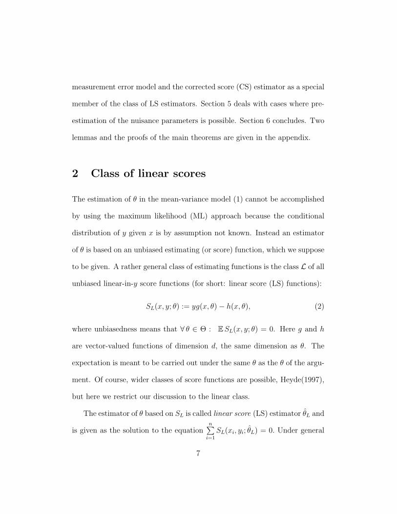
measurement error model and the corrected score (CS) estimator as a special

member of the class of LS estimators. Section 5 deals with cases where pre-

estimation of the nuisance parameters is possible. Section 6 concludes. Two

lemmas and the proofs of the main theorems are given in the appendix.

2 Class of linear scores

The estimation of θ in the mean-variance model (1) cannot be accomplished

by using the maximum likelihood (ML) approach because the conditional

distribution of y given x is by assumption not known. Instead an estimator

of θ is based on an unbiased estimating (or score) function, which we suppose

to be given. A rather general class of estimating functions is the class L of all

unbiased linear-in-y score functions (for short: linear score (LS) functions):

SL(x, y; θ) := yg(x, θ)− h(x, θ), (2)

where unbiasedness means that ∀ θ ∈ Θ : ESL(x, y; θ) = 0. Here g and h

are vector-valued functions of dimension d, the same dimension as θ. The

expectation is meant to be carried out under the same θ as the θ of the argu-

ment. Of course, wider classes of score functions are possible, Heyde(1997),

but here we restrict our discussion to the linear class.

The estimator of θ based on SL is called linear score (LS) estimator θL and

is given as the solution to the equationn∑i=1

SL(xi, yi; θL) = 0. Under general

7

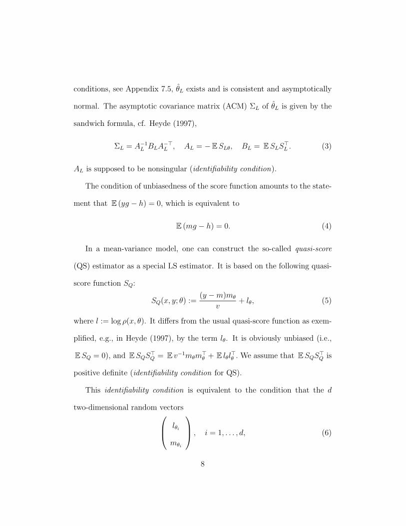
conditions, see Appendix 7.5, θL exists and is consistent and asymptotically

normal. The asymptotic covariance matrix (ACM) ΣL of θL is given by the

sandwich formula, cf. Heyde (1997),

ΣL = A−1L BLA

−>L , AL = −ESLθ, BL = ESLS>L . (3)

AL is supposed to be nonsingular (identifiability condition).

The condition of unbiasedness of the score function amounts to the state-

ment that E (yg − h) = 0, which is equivalent to

E (mg − h) = 0. (4)

In a mean-variance model, one can construct the so-called quasi-score

(QS) estimator as a special LS estimator. It is based on the following quasi-

score function SQ:

SQ(x, y; θ) :=(y −m)mθ

v+ lθ, (5)

where l := log ρ(x, θ). It differs from the usual quasi-score function as exem-

plified, e.g., in Heyde (1997), by the term lθ. It is obviously unbiased (i.e.,

ESQ = 0), and ESQS>Q = E v−1mθm>θ + E lθl>θ . We assume that ESQS>Q is

positive definite (identifiability condition for QS).

This identifiability condition is equivalent to the condition that the d

two-dimensional random vectors lθi

mθi

, i = 1, . . . , d, (6)

8

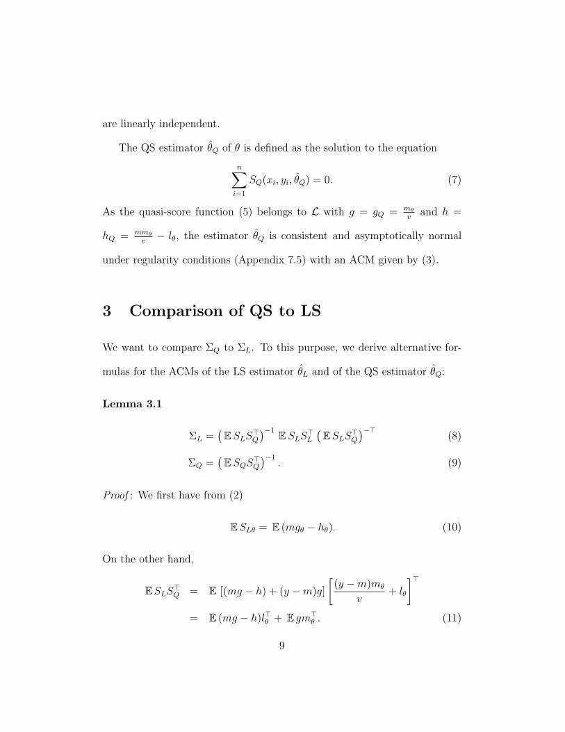
are linearly independent.

The QS estimator θQ of θ is defined as the solution to the equation

n∑i=1

SQ(xi, yi, θQ) = 0. (7)

As the quasi-score function (5) belongs to L with g = gQ = mθv

and h =

hQ = mmθv− lθ, the estimator θQ is consistent and asymptotically normal

under regularity conditions (Appendix 7.5) with an ACM given by (3).

3 Comparison of QS to LS

We want to compare ΣQ to ΣL. To this purpose, we derive alternative for-

mulas for the ACMs of the LS estimator θL and of the QS estimator θQ:

Lemma 3.1

ΣL =(

ESLS>Q)−1 ESLS>L

(ESLS>Q

)−>(8)

ΣQ =(

ESQS>Q)−1

. (9)

Proof : We first have from (2)

ESLθ = E (mgθ − hθ). (10)

On the other hand,

ESLS>Q = E [(mg − h) + (y −m)g]

[(y −m)mθ

v+ lθ

]>= E (mg − h)l>θ + E gm>θ . (11)

9

We can derive the following identity from (4):

E (mg − h)θ + E (mg − h)l>θ = 0. (12)

From (10), (11), and (12) we obtain

ESLθ + ESLS>Q = E (mg − h)θ + E (mg − h)l>θ = 0,

which yields

ESLθ = −ESLS>Q . (13)

Now, (13) implies that the ACM of θL, given by (3), can be written as in

(8). Finally, as SQ belongs to L, we can apply (8) to SQ and obtain (9) for

the ACM of θQ. This completes the proof.

We now can state the following theorems.

Theorem 3.1 (Optimality of QS) Let SL be a score function from the

class L and SQ be the quasi-score function (5). Then

ΣQ ≤ ΣL.

Moreover, ΣL = ΣQ for all θ if, and only if, θL = θQ a.s.

Remark 1. Depending on the model involved, there may be other estimators

that are more efficient than QS (e.g., ML), but according to the theorem

they would imply a non-linear-in-y score function.

10

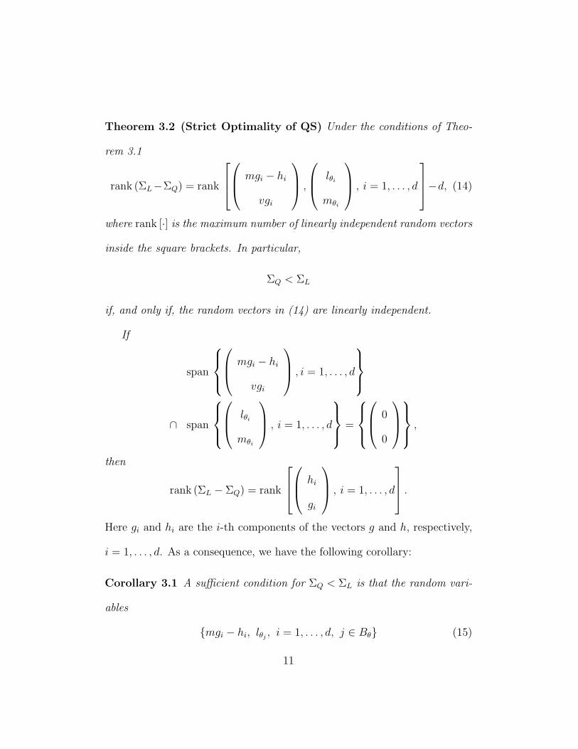
Theorem 3.2 (Strict Optimality of QS) Under the conditions of Theo-

rem 3.1

rank (ΣL−ΣQ) = rank

mgi − hi

vgi

,

lθi

mθi

, i = 1, . . . , d

−d, (14)

where rank [·] is the maximum number of linearly independent random vectors

inside the square brackets. In particular,

ΣQ < ΣL

if, and only if, the random vectors in (14) are linearly independent.

If

span

mgi − hi

vgi

, i = 1, . . . , d

∩ span

lθi

mθi

, i = 1, . . . , d

=

0

0

,

then

rank (ΣL − ΣQ) = rank

hi

gi

, i = 1, . . . , d

.Here gi and hi are the i-th components of the vectors g and h, respectively,

i = 1, . . . , d. As a consequence, we have the following corollary:

Corollary 3.1 A sufficient condition for ΣQ < ΣL is that the random vari-

ables

{mgi − hi, lθj , i = 1, . . . , d, j ∈ Bθ} (15)

11

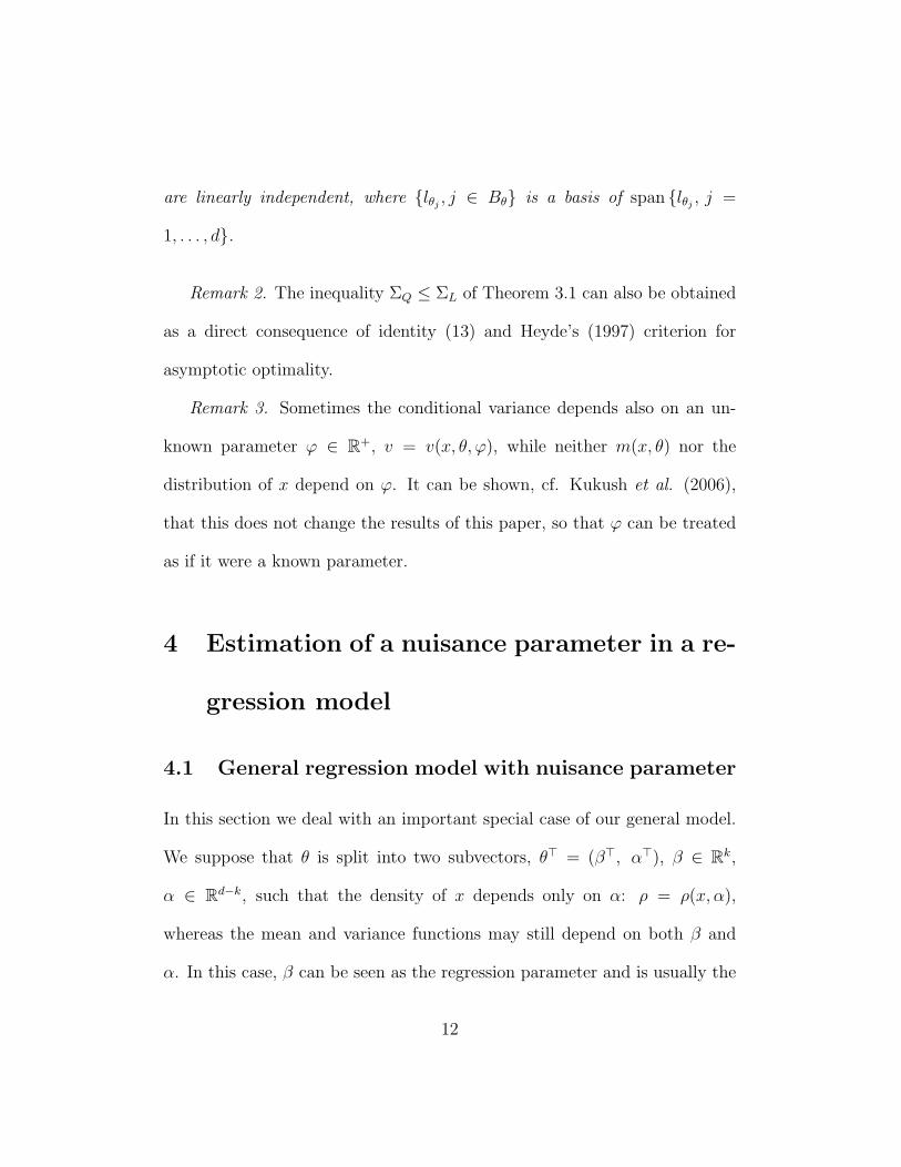
are linearly independent, where {lθj , j ∈ Bθ} is a basis of span {lθj , j =

1, . . . , d}.

Remark 2. The inequality ΣQ ≤ ΣL of Theorem 3.1 can also be obtained

as a direct consequence of identity (13) and Heyde’s (1997) criterion for

asymptotic optimality.

Remark 3. Sometimes the conditional variance depends also on an un-

known parameter ϕ ∈ R+, v = v(x, θ, ϕ), while neither m(x, θ) nor the

distribution of x depend on ϕ. It can be shown, cf. Kukush et al. (2006),

that this does not change the results of this paper, so that ϕ can be treated

as if it were a known parameter.

4 Estimation of a nuisance parameter in a re-

gression model

4.1 General regression model with nuisance parameter

In this section we deal with an important special case of our general model.

We suppose that θ is split into two subvectors, θ> = (β>, α>), β ∈ Rk,

α ∈ Rd−k, such that the density of x depends only on α: ρ = ρ(x, α),

whereas the mean and variance functions may still depend on both β and

α. In this case, β can be seen as the regression parameter and is usually the

12

parameter of interest, while α is a nuisance parameter.

The quasi-score function (5) takes the form

SQ =

(y −m)v−1mβ

(y −m)v−1mα + lα

. (16)

Such a model arises naturally in the context of measurement error models,

see Section 4.2. All the previous results hold true.

We obtain more detailed results if, corresponding to the special QS func-

tion (16), we also choose a special subclass L∗ ⊂ L, to which (16) can then

be compared. The corrected score function of the next subsection will be an

example of an element of L∗. Assume that SL is of the form

SL =

yg(x, β)− h(x, β)

lα

, (17)

where now g and h are of dimension k and do not depend on α. Unbiasedness

of SL again means that E(mg − h) = 0 because E lα = 0 anyway. Note that

SQ is not a member of this restricted class. Nevertheless, we can still apply

Theorems 3.1 and 3.2 with L replaced by L∗ to compare ΣL to ΣQ. In

particular, the first part of Theorem 3.2 takes the form:

Theorem 4.1 If θ = (β>, α>)> and ρ = ρ(x, α) and SL is of the form (17),

13

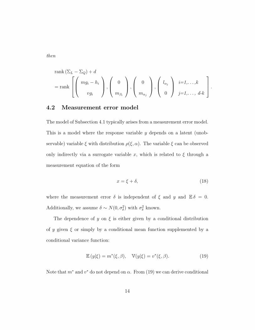
then

rank (ΣL − ΣQ) + d

= rank

mgi − hi

vgi

,

0

mβi

,

0

mαj

,

lαj

0

i=1,. . . ,k

j=1,. . . , d-k

.4.2 Measurement error model

The model of Subsection 4.1 typically arises from a measurement error model.

This is a model where the response variable y depends on a latent (unob-

servable) variable ξ with distribution ρ(ξ, α). The variable ξ can be observed

only indirectly via a surrogate variable x, which is related to ξ through a

measurement equation of the form

x = ξ + δ, (18)

where the measurement error δ is independent of ξ and y and E δ = 0.

Additionally, we assume δ ∼ N(0, σ2δ ) with σ2

δ known.

The dependence of y on ξ is either given by a conditional distribution

of y given ξ or simply by a conditional mean function supplemented by a

conditional variance function:

E (y|ξ) = m∗(ξ, β), V(y|ξ) = v∗(ξ, β). (19)

Note that m∗ and v∗ do not depend on α. From (19) we can derive conditional

14

mean and variance functions of y given x, which do depend on α:

m(x, β, α) := E (y|x) = E [m∗(ξ, β)|x] (20)

v(x, β, α) := V(y|x) = E [v∗(ξ, β)|x] + V[m∗(ξ, β)|x]. (21)

To compute these, we need to know the conditional distribution of ξ given

x, which we can derive from the unconditional distribution of ξ, ρ(ξ, α), and

the measurement equation (18). An example is the normal distribution in

Sections 5.2 and 5.3.

Among the linear score functions, the so-called corrected score (CS) func-

tion is of particular interest. It is given by special functions g and h. Suppose

we can find functions g = g(x, β) and h = h(x, β) such that

E [g|ξ] = v∗−1m∗β (22)

E [h|ξ] = m∗v∗−1m∗β. (23)

Then, because of E (yg − h) = E E [(yg − h)|y, ξ] = E (y −m∗)v∗−1m∗β = 0,

SC :=

yg − h

lα

is a linear score function within the class L∗. It is called the corrected score

function of the measurement error model. For this score function, Theorem

4.1 applies with SC in place of SL. In a number of important cases (like the

Poisson, the gamma, and the Gaussian polynomial model) such functions g

15

and h can be found in closed form, see Sections 5.3 and 5.4. But there are

also cases where g and h do not exist, Stefanski (1989).

5 Pre-estimation of nuisance parameters

5.1 General model

In the model of Section 4.1 with θ> = (β>, α>), we could also define a

modified QS estimator, which is based on a score function that instead of (16)

consists of the two subvectors (y −m)v−1mβ and lα, implying an estimator

of α which uses the second subvector only. This means that α would be pre-

estimated using only the data xi, not the data yi. We can then substitute

the resulting estimator α in the first subvector, (y −m)v−1mβ, and use this

to estimate β. We might call this estimator of β a QS estimator with pre-

estimated nuisance parameters or simply pre-estimated QS estimator.

Such a two-step estimation procedure is, of course, simpler to apply than

the one we propose, but according to Theorem 3.1 it is at most as efficient

and often less efficient than the latter one.

There are, however, cases where pre-estimation of the nuisance parameter

is in accordance with our QS approach and does not reduce the efficiency of

QS. Suppose that

mα = Amβ (24)

16

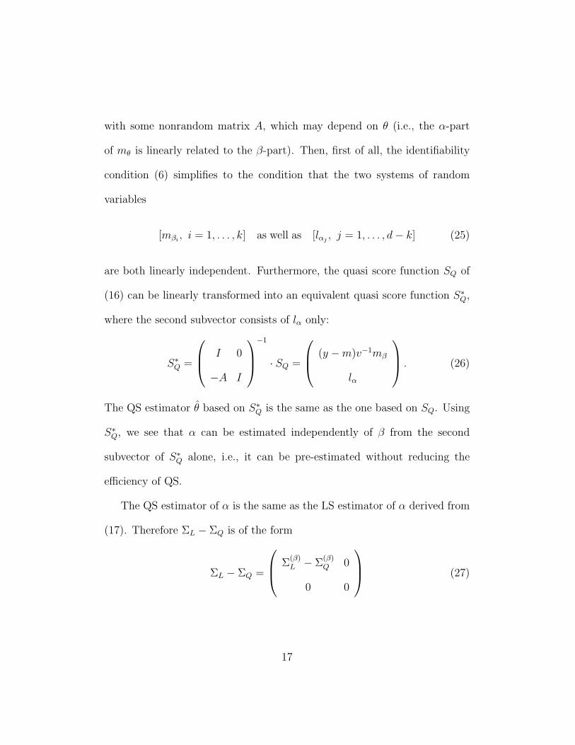
with some nonrandom matrix A, which may depend on θ (i.e., the α-part

of mθ is linearly related to the β-part). Then, first of all, the identifiability

condition (6) simplifies to the condition that the two systems of random

variables

[mβi , i = 1, . . . , k] as well as [lαj , j = 1, . . . , d− k] (25)

are both linearly independent. Furthermore, the quasi score function SQ of

(16) can be linearly transformed into an equivalent quasi score function S∗Q,

where the second subvector consists of lα only:

S∗Q =

I 0

−A I

−1

· SQ =

(y −m)v−1mβ

lα

. (26)

The QS estimator θ based on S∗Q is the same as the one based on SQ. Using

S∗Q, we see that α can be estimated independently of β from the second

subvector of S∗Q alone, i.e., it can be pre-estimated without reducing the

efficiency of QS.

The QS estimator of α is the same as the LS estimator of α derived from

(17). Therefore ΣL − ΣQ is of the form

ΣL − ΣQ =

Σ(β)L − Σ

(β)Q 0

0 0

(27)

17

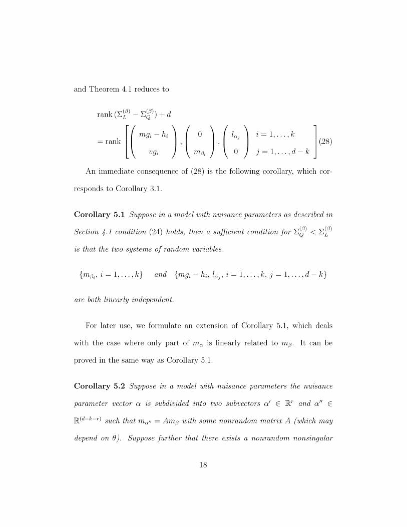
and Theorem 4.1 reduces to

rank (Σ(β)L − Σ

(β)Q ) + d

= rank

mgi − hi

vgi

,

0

mβi

,

lαj

0

i = 1, . . . , k

j = 1, . . . , d− k

.(28)

An immediate consequence of (28) is the following corollary, which cor-

responds to Corollary 3.1.

Corollary 5.1 Suppose in a model with nuisance parameters as described in

Section 4.1 condition (24) holds, then a sufficient condition for Σ(β)Q < Σ

(β)L

is that the two systems of random variables

{mβi , i = 1, . . . , k} and {mgi − hi, lαj , i = 1, . . . , k, j = 1, . . . , d− k}

are both linearly independent.

For later use, we formulate an extension of Corollary 5.1, which deals

with the case where only part of mα is linearly related to mβ. It can be

proved in the same way as Corollary 5.1.

Corollary 5.2 Suppose in a model with nuisance parameters the nuisance

parameter vector α is subdivided into two subvectors α′ ∈ Rr and α′′ ∈

R(d−k−r) such that mα′′ = Amβ with some nonrandom matrix A (which may

depend on θ). Suppose further that there exists a nonrandom nonsingular

18

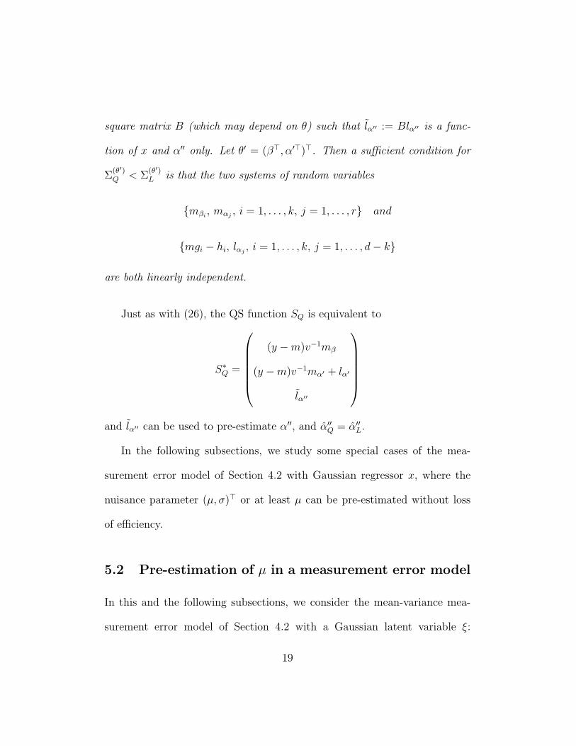
square matrix B (which may depend on θ) such that lα′′ := Blα′′ is a func-

tion of x and α′′ only. Let θ′ = (β>, α′>)>. Then a sufficient condition for

Σ(θ′)Q < Σ

(θ′)L is that the two systems of random variables

{mβi , mαj , i = 1, . . . , k, j = 1, . . . , r} and

{mgi − hi, lαj , i = 1, . . . , k, j = 1, . . . , d− k}

are both linearly independent.

Just as with (26), the QS function SQ is equivalent to

S∗Q =

(y −m)v−1mβ

(y −m)v−1mα′ + lα′

lα′′

and lα′′ can be used to pre-estimate α′′, and α′′Q = α′′L.

In the following subsections, we study some special cases of the mea-

surement error model of Section 4.2 with Gaussian regressor x, where the

nuisance parameter (µ, σ)> or at least µ can be pre-estimated without loss

of efficiency.

5.2 Pre-estimation of µ in a measurement error model

In this and the following subsections, we consider the mean-variance mea-

surement error model of Section 4.2 with a Gaussian latent variable ξ:

19

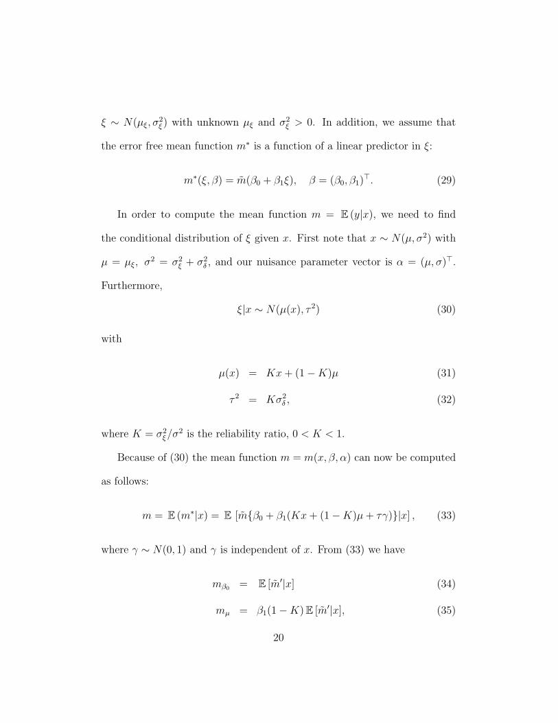
ξ ∼ N(µξ, σ2ξ ) with unknown µξ and σ2

ξ > 0. In addition, we assume that

the error free mean function m∗ is a function of a linear predictor in ξ:

m∗(ξ, β) = m(β0 + β1ξ), β = (β0, β1)>. (29)

In order to compute the mean function m = E (y|x), we need to find

the conditional distribution of ξ given x. First note that x ∼ N(µ, σ2) with

µ = µξ, σ2 = σ2

ξ + σ2δ , and our nuisance parameter vector is α = (µ, σ)>.

Furthermore,

ξ|x ∼ N(µ(x), τ 2) (30)

with

µ(x) = Kx+ (1−K)µ (31)

τ 2 = Kσ2δ , (32)

where K = σ2ξ/σ

2 is the reliability ratio, 0 < K < 1.

Because of (30) the mean function m = m(x, β, α) can now be computed

as follows:

m = E (m∗|x) = E [m{β0 + β1(Kx+ (1−K)µ+ τγ)}|x] , (33)

where γ ∼ N(0, 1) and γ is independent of x. From (33) we have

mβ0 = E [m′|x] (34)

mµ = β1(1−K) E [m′|x], (35)

20

where ′ denotes the derivative and m′ is short for m′{β0 +β1(Kx+(1−K)µ+

τγ)} . Thus

mµ = β1(1−K)mβ0 . (36)

This corresponds to the equation mα′′ = Amβ of Corollary 5.2 with α′′ = µ,

and hence µ can be pre-estimated. Indeed, SQ is equivalent to

S∗Q =

(y −m)v−1mβ

(y −m)v−1mσ + lσ

lµ

, (37)

where

lα = (lµ, lσ)> =

(x− µσ2

,(x− µ)2

σ3− 1

σ

)>. (38)

Thus, for a linear predictor mean-variance measurement error model with

Gaussian regressor, µ can be pre-estimated by using the score function lµ,

i.e., by solving the estimating equation∑n

i=1xi−µσ2 = 0 with the solution

µQ = x := 1n

∑ni=1 xi.

5.3 Pre-estimation of σ in a measurement error model

Continuing with the model of Section 5.2, we now derive conditions under

which not only µ but also σ can be pre-estimated without loss of efficiency.

Starting from (33), we find, in addition to (34) and (35),

21

mβ1 = (Kx+ (1−K)µ) E [m′|x] + β1τ2 E [m′′|x] , (39)

mσ = β1Kσ(x− µ) E [m′|x] + β21ττσ E [m′′|x] . (40)

Here we used the identity

E [m′(a+ bγ)γ|x] = bE [m′′(a+ bγ)|x] ,

where a = a(x) and b = b(x) are any functions of x. Indeed, by partial

integration,

E [m′(a+ bγ)γ|x] =

∫m′(a+ bγ)γq(γ)dγ = b

∫m′′(a+ bγ)q(γ)dγ

= bE [m′′(a+ bγ)|x] ,

where q(γ) is the density of the standard normal distribution.

Now suppose that the following differential equation holds for m:

m′′ = c0m′ (41)

with some constant c0. Then by (34), (39), (40),and (41) and because K > 0,

mσ = d1mβ0 + d2mβ1

with some constants d1 and d2. Thus

mα = (mµ,mσ)> = A(mβ0 ,mβ1)> = Amβ

22

with some constant (2× 2)-matrix A, and, according to Section 5.1, µ and σ

can be pre-estimated. The QS estimates of µ and σ are simply the empirical

mean and variance of the data xi:

µQ = x, σ2Q = s2

x :=1

n

n∑i=1

(xi − x)2.

The linear differential equation (41) has the solution

m(t) = c1ec0t + c2. (42)

An example is the log-linear Poisson model with measurement errors and

Gaussian regressor. It is given by y|ξ ∼ Po(λ) with λ = exp(β0 + β1ξ), and

x = ξ + δ. Here m∗ = λ and m(t) = et, which satisfies (42). For this model

µ and σ can be pre-estimated. The exponential model y|ξ ∼ Exp(λ) with

λ = exp(β0 + β1ξ) is another example and so is the more general gamma

model, Kukush et al.(2008).

As a further example we study the polynomial measurement error model

in some detail in the next subsection, where again µ and σ can be pre-

estimated, but for different reasons.

5.4 Polynomial measurement error model

The polynomial measurement error model of degree k is given by y = β>ζ+ε

and x = ξ + δ with ζ = ζ(ξ) = (1, ξ, . . . , ξk)> and β = (β0, β1 . . . , βk)>. The

variable ε is independent of ξ and δ, and all variables are Gaussian. In

23

particular, as before, x ∼ N(µ, σ2), where the nuisance parameters µ and σ

are supposed to be unknown.

Clearly, m∗(ξ, β) = β>ζ(ξ) and v∗ = σ2ε . (σ2

ε is a dispersion parameter,

which we can assume to be known when we are only interested in comparing

the ACMs of βC and βQ, see Remark 3). It follows that

m = β> E (ζ|x), mβ = E (ζ|x), mµ = (1−K)β> E (ζ ′|x),

where ζ ′ is the derivative of ζ. Now there is a constant square matrix D such

that

ζ ′(ξ) = Dζ(ξ), (43)

and so

mµ = (1−K)β>Dmβ.

Therefore, according to Section 5.1, µ can be pre-estimated and µQ = x.

Considering the nuisance parameter σ, we can show by similar arguments

as those that led to (40) that

mσ = β> (Kσ(x− µ) E [ζ ′|x] + ττσ E [ζ ′′|x]) .

We see that mσ is a polynomial function of x of degree k, while the com-

ponents of E (ζ|x), i.e., E [ξj|x], are polynomials of degree j, j = 0, . . . , k.

Therefore mσ is a linear combination of the components of E (ζ|x) (with co-

efficients depending on µ, σ, and β). Thus mσ = b>mβ with some constant

24

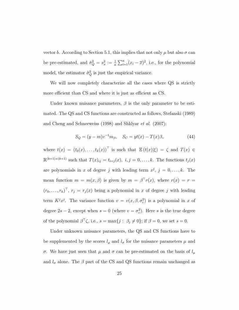
vector b. According to Section 5.1, this implies that not only µ but also σ can

be pre-estimated, and σ2Q = s2

x := 1n

∑ni=1(xi − x)2, i.e., for the polynomial

model, the estimator σ2Q is just the empirical variance.

We will now completely characterize all the cases where QS is strictly

more efficient than CS and where it is just as efficient as CS.

Under known nuisance parameters, β is the only parameter to be esti-

mated. The QS and CS functions are constructed as follows, Stefanski (1989)

and Cheng and Schneeweiss (1998) and Shklyar et al. (2007):

SQ = (y −m)v−1mβ, SC = yt(x)− T (x)β, (44)

where t(x) = (t0(x), . . . , tk(x))> is such that E (t(x)|ξ) = ζ and T (x) ∈

R(k+1)×(k+1) such that T (x)ij = ti+j(x), i, j = 0, . . . , k. The functions tj(x)

are polynomials in x of degree j with leading term xj, j = 0, . . . , k. The

mean function m = m(x, β) is given by m = β>r(x), where r(x) = r =

(r0, . . . , rk)>, rj = rj(x) being a polynomial in x of degree j with leading

term Kjxj. The variance function v = v(x, β, σ2ε) is a polynomial in x of

degree 2s− 2, except when s = 0 (where v = σ2ε). Here s is the true degree

of the polynomial β>ζ, i.e., s = max{j : βj 6= 0}; if β = 0, we set s = 0.

Under unknown nuisance parameters, the QS and CS functions have to

be supplemented by the scores lµ and lσ for the nuisance parameters µ and

σ. We have just seen that µ and σ can be pre-estimated on the basis of lµ

and lσ alone. The β part of the CS and QS functions remain unchanged as

25

in (44) except that µ and σ are replaced with their estimates.

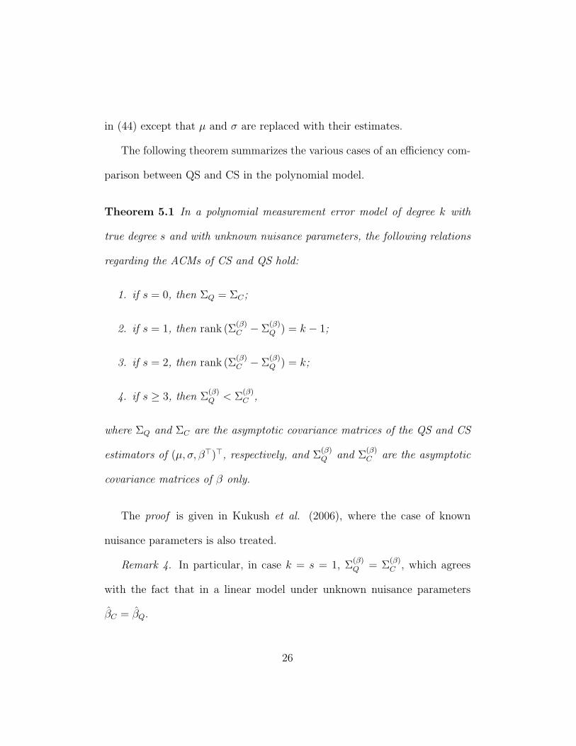
The following theorem summarizes the various cases of an efficiency com-

parison between QS and CS in the polynomial model.

Theorem 5.1 In a polynomial measurement error model of degree k with

true degree s and with unknown nuisance parameters, the following relations

regarding the ACMs of CS and QS hold:

1. if s = 0, then ΣQ = ΣC;

2. if s = 1, then rank (Σ(β)C − Σ

(β)Q ) = k − 1;

3. if s = 2, then rank (Σ(β)C − Σ

(β)Q ) = k;

4. if s ≥ 3, then Σ(β)Q < Σ

(β)C ,

where ΣQ and ΣC are the asymptotic covariance matrices of the QS and CS

estimators of (µ, σ, β>)>, respectively, and Σ(β)Q and Σ

(β)C are the asymptotic

covariance matrices of β only.

The proof is given in Kukush et al. (2006), where the case of known

nuisance parameters is also treated.

Remark 4. In particular, in case k = s = 1, Σ(β)Q = Σ

(β)C , which agrees

with the fact that in a linear model under unknown nuisance parameters

βC = βQ.

26

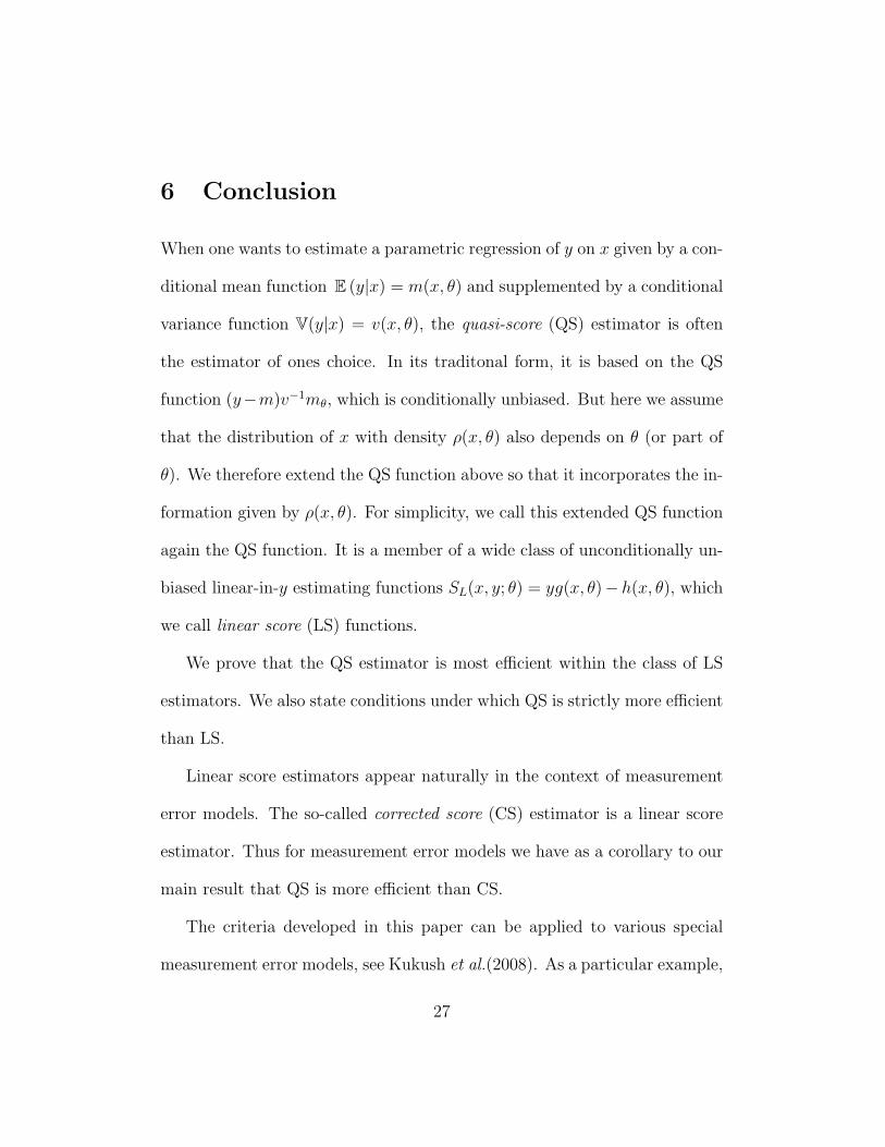
6 Conclusion

When one wants to estimate a parametric regression of y on x given by a con-

ditional mean function E (y|x) = m(x, θ) and supplemented by a conditional

variance function V(y|x) = v(x, θ), the quasi-score (QS) estimator is often

the estimator of ones choice. In its traditonal form, it is based on the QS

function (y−m)v−1mθ, which is conditionally unbiased. But here we assume

that the distribution of x with density ρ(x, θ) also depends on θ (or part of

θ). We therefore extend the QS function above so that it incorporates the in-

formation given by ρ(x, θ). For simplicity, we call this extended QS function

again the QS function. It is a member of a wide class of unconditionally un-

biased linear-in-y estimating functions SL(x, y; θ) = yg(x, θ)− h(x, θ), which

we call linear score (LS) functions.

We prove that the QS estimator is most efficient within the class of LS

estimators. We also state conditions under which QS is strictly more efficient

than LS.

Linear score estimators appear naturally in the context of measurement

error models. The so-called corrected score (CS) estimator is a linear score

estimator. Thus for measurement error models we have as a corollary to our

main result that QS is more efficient than CS.

The criteria developed in this paper can be applied to various special

measurement error models, see Kukush et al.(2008). As a particular example,

27

the polynomial measurement error model has been studied in the present

paper.

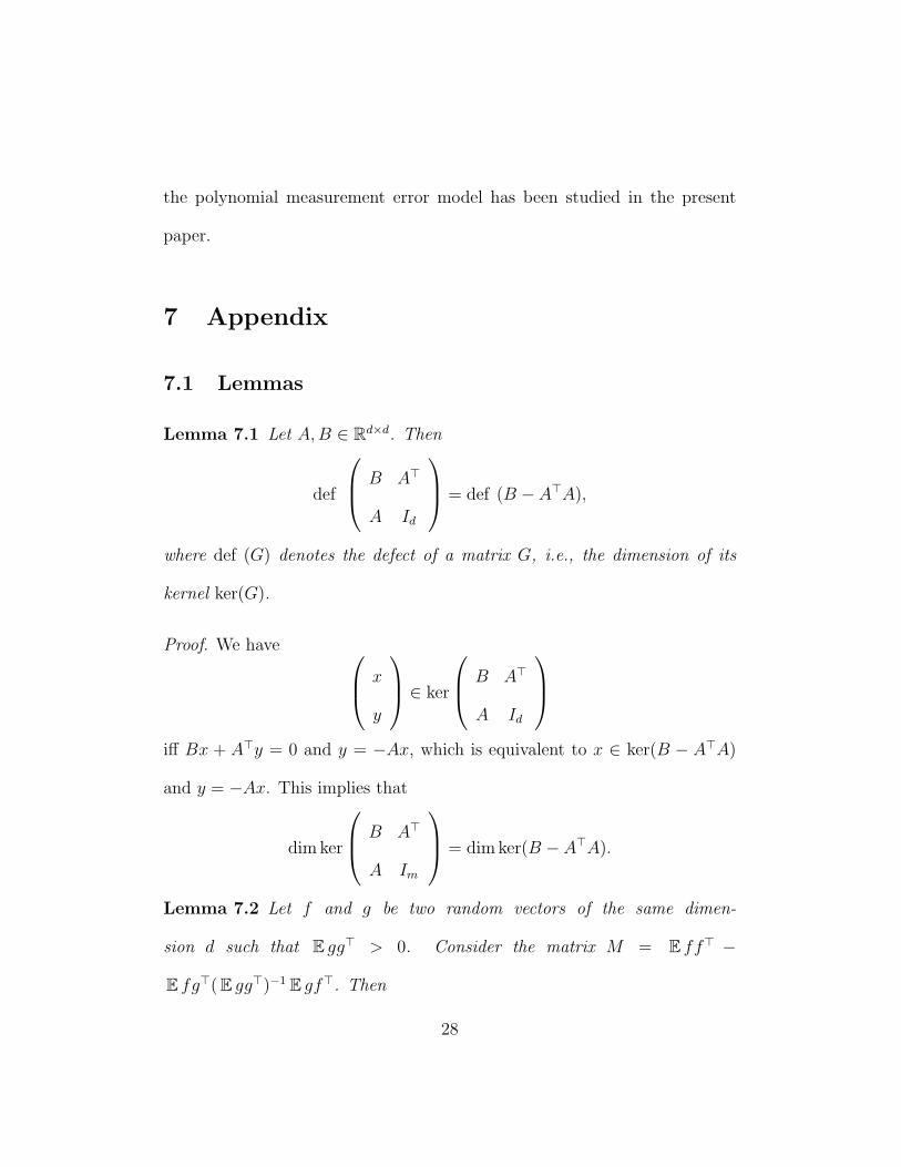
7 Appendix

7.1 Lemmas

Lemma 7.1 Let A,B ∈ Rd×d. Then

def

B A>

A Id

= def (B − A>A),

where def (G) denotes the defect of a matrix G, i.e., the dimension of its

kernel ker(G).

Proof. We have x

y

∈ ker

B A>

A Id

iff Bx + A>y = 0 and y = −Ax, which is equivalent to x ∈ ker(B − A>A)

and y = −Ax. This implies that

dim ker

B A>

A Im

= dim ker(B − A>A).

Lemma 7.2 Let f and g be two random vectors of the same dimen-

sion d such that E gg> > 0. Consider the matrix M = E ff> −

E fg>( E gg>)−1 E gf>. Then

28

1) M is positive semi-definite. Moreover, M is the zero matrix if, and

only if, f = Hg a.s., with some nonrandom square matrix H;

2) rankM = rank [fi, gi, i = 1, . . . , d] − d, where the latter rank is the

maximum number of linearly independent random variables in the set

{fi, gi, i = 1, . . . , d}.

Proof. 1) To prove the first statement, let

e = f − E fg>( E gg>)−1g.

Then E ee> = M ≥ 0, and M = 0 iff e = 0, that is, iff f = Hg with some

nonrandom square matrix H.

2) To prove the second statement, let

F = E ff>, g = ( E gg>)−1/2g, A = E gf>.

Then M = (F − A>A) and, by Lemma 7.1,

rankM = rank [F − A>A] = rank

F A>

A Id

− d.The latter rank is the rank of the moment matrix of the random vector

[f1, . . . , fd, g1, . . . , gd]. It is therefore equal to the rank of this vector. But

due to the definition of g,

rank [f1, . . . , fd, g1, . . . , gd] = rank [f1, . . . , fd, g1, . . . , gd].

29

7.2 Proof of Theorem 3.1

We apply the first statement of Lemma 7.2 to the random vectors g = SQ

and f = SL. We have

E ff> − E fg>(

E gg>)−1 E gf> ≥ 0.

Due to (8) and (9) this is equivalent to ΣL − ΣQ ≥ 0. Equality between

ΣL and ΣQ for all θ holds iff for some nonrandom square matrix H = H(θ),

f = Hg, i.e.,

∀ θ : SL = H(θ)SQ a.s.

Because ESLS>Q is nonsingular, H is nonsingular as well. Then the equation

for θL,∑n

i=1 SL(xi, yi; θ) = 0, is equivalent to∑n

i=1 H(θ)SQ(xi, yi; θ) = 0,

which is a.s. equivalent to the equation for θQ,∑n

i=1 SQ(xi, yi; θ) = 0. Thus

θL = θQ a.s.

Vice versa, if θL = θQ a.s., then ΣL = ΣQ for all θ.

7.3 Proof of Theorem 3.2

We apply the second statement of Lemma 7.2 with g = SQ, f = SL. By (8)

and (9),

rank (ΣL − ΣQ) = rankM = rank [(SL)i, (SQ)i, i = 1, . . . , d]− d

= d− def [(SL)i, (SQ)i, i = 1, . . . , d] . (45)

30

To find the defect, we form a linear combination of the components of SL

and SQ, see (2) and (5), which is supposed to equal zero a.s.:

c>1 gy − c>1 h+c>2 mθ

v(y −m) + c>2 lθ = 0 a.s.

or (c>1 g +

c>2 mθ

v

)y = c>1 h+

c>2 mmθ

v− c>2 lθ a.s. (46)

The defect in (45) is equal to the maximum number of linearly independent

vectors (c>1 , c>2 )> which satisfy (46). But (46) is equivalent to

c>1 g +c>2 mθ

v= 0 and c>1 h+

c>2 mmθ

v− c>2 lθ = 0 a.s. (47)

Indeed in general, a(x)y = b(x) a.s. implies a2(x)v(x) = 0 and therefore

a(x) = 0 because by assumption v(x) > 0. Now, (47) is equivalent to

c>1 vg + c>2 mθ = 0, c>1 (mg − h) + c>2 lθ = 0 a.s.

Thus

def [(SL)i, (SQ)i, i = 1, . . . , d]

= def

mgi − hi

vgi

,

lθi

mθi

, i = 1, . . . , d

,and (14) follows from (45).

31

7.4 Proof of Corollary 3.1

Suppose the random variables (15) are linearly independent. Then because of

the identifiability condition (6), the random vectors in (14) are also linearly

independent. Indeed, for any constant vectors a and b ∈ Rd, the system of

equations

a>(mg − h) + b>lθ = 0

a>vg + b>mθ = 0

implies first a = 0 because of the independence of the random variables in

(15) and then b = 0 because of (6). According to Theorem 3.2, it follows

that ΣQ < ΣL.

7.5 Consistency and asymptotic normality of θL

Lemma 7.3 Consider model (1) of the Introduction and assume the follow-

ing conditions.

1. The parameter set Θ is a convex compact set in Rd, and the true pa-

rameter value θ lies in Θ◦, the interior of Θ.

2. The functions g,h: R× U → Rd of (2) are Borel measurable, where U

is a neighborhood of Θ, moreover, g(x, ·) and h(x, ·) belong to C2(U)

a.s.

32

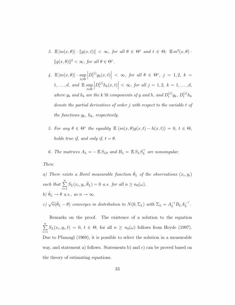
3. E |m(x, θ)| · ‖g(x, t)‖ < ∞, for all θ ∈ Θ◦ and t ∈ Θ; Em2(x, θ) ·

‖g(x, θ)‖2 <∞, for all θ ∈ Θ◦.

4. E |m(x, θ)| · supt∈Θ

∣∣∣D(j)t gk(x, t)

∣∣∣ < ∞, for all θ ∈ Θ◦, j = 1, 2, k =

1, . . . , d, and E supt∈Θ

∣∣∣D(j)t hk(x, t)

∣∣∣ < ∞, for all j = 1, 2, k = 1, . . . , d,

where gk and hk are the k’th components of g and h, and D(j)t gk, D

(j)t hk

denote the partial derivatives of order j with respect to the variable t of

the functions gk, hk, respectively.

5. For any θ ∈ Θ◦ the equality E (m(x, θ)g(x, t)− h(x, t)) = 0, t ∈ Θ,

holds true if, and only if, t = θ.

6. The matrices AL = −ESLθ and BL = ESLS>L are nonsingular.

Then:

a) There exists a Borel measurable function θL of the observations (xi, yi)

such thatn∑i=1

SL(xi, yi, θL) = 0 a.s. for all n ≥ n0(ω).

b) θL → θ a.s., as n→∞.

c)√n(θL − θ) converges in distribution to N(0,ΣL) with ΣL = A−1

L BLA−>L .

Remarks on the proof. The existence of a solution to the equationn∑i=1

SL(xi, yi, t) = 0, t ∈ Θ, for all n ≥ n0(ω) follows from Heyde (1997).

Due to Pfanzagl (1969), it is possible to select the solution in a measurable

way, and statement a) follows. Statements b) and c) can be proved based on

the theory of estimating equations.

33

References

[1] Armstrong, B. (1985), Measurement error in the generalized linear

model. Comm. Statist. Simulation Comput. 14, 529-544.

[2] Carroll, R. J., Ruppert, D., Stefanski, L.A., and Crainiceanu, C. M.

(2006), Measurement Error in Nonlinear Models. Chapman and Hall,

London.

[3] Cheng, C.-L. and Van Ness, J. W., (1999), Statistical Regression with

Measurement Error. Arnold, London.

[4] Cheng, C.-L. and Schneeweiss, H. (1998), Polynomial regression with

errors in the variables. J. Roy. Statist. Soc. Ser. B 60, 189 - 199.

[5] Fuller, W. A. (1987), Measurement Error Models. Wiley, New York.

[6] Heyde, C. C. (1997), Quasi-Likelihood And Its Application. Springer,

New York.

[7] Kukush, A. and Schneeweiss H. (2005), Comparing different estimators

in a nonlinear measurement error model. I. Math. Methods Statist. 14,

53-79.

34

[8] Kukush, A. and Schneeweiss H. (2006), Asymptotic optimality of the

quasi-score estimator in a class of linear score estimators, Discussion

Paper 477, SFB 386, Universitat Munchen.

[9] Kukush, A., Malenko A., and Schneeweiss H. (2006),Optimality of the

quasi-score estimator in a mean-variance model with applications to

measurement error models. Discussion Paper 494, SFB 386, University

of Munich.

[10] Kukush, A., Malenko A., and Schneeweiss H. (2007), Comparing the

efficiency of estimates in concrete errors-in-variables models under un-

known nuisance parameters. Theory of Stochastic Processes 13 (29),

69-81.

[11] Nakamura, T. (1990), Corrected score function for errors-in-variables

models. Biometrika 77, 127-137.

[12] Pfanzagl, G. (1969), On the measurability and consistency of minimum

contrast estimates. Metrika 14, 249-273.

[13] Schervish, M.J. (1995), Theory of Statistics. Springer, New York.

[14] Shklyar, S., Schneeweiss, H., and Kukush, A. (2007), Quasi Score is

more efficient than Corrected Score in a polynomial measurement error

model. Metrika 65, 275-295.

35

[15] Stefanski, L. (1989), Unbiased estimation of a nonlinear function of a

normal mean with application to measurement error models. Comm.

Statist. Theory Methods 18, 4335-4358.

[16] Wedderburn, R.W.M. (1974), Quasi likelihood functions, generalized

linear models, and the Gauss-Newton method. Biometrika 61, 439-447.

Addresses:

Alexander Kukush: Department of Mechanics and Mathematics, Kiev

National Taras Shevchenko University, Volodymyrska str. 60, 01033 Kiev,

Ukraine. E-mail: alexander [email protected]

Andrii Malenko: Department of Mechanics and Mathematics, Kiev Na-

tional Taras Shevchenko University, Volodymyrska str. 60, 01033 Kiev,

Ukraine. E-mail: [email protected]

Hans Schneeweiss: Department of Statistics, University of Munich,

Akademiestr. 1, 80799 Munich, Germany. E-mail: [email protected]

muenchen.de

36