Optimal Timing for an Asset Sale in an Incomplete Market Timing for an Asset Sale in an Incomplete Market Jonathan Evansy University of Bath Vicky Hendersonz Princeton University David

Optimal Timing for an Asset Sale in an

Incomplete Market

Jonathan Evans†

University of Bath

Vicky Henderson‡

Princeton University

David Hobson§

University of Bath

First version: February 2005;This version: November 24, 2005

Abstract

In this paper we investigate the pricing via utility indifference of the right to sell

a non-traded asset.

Consider an agent with power utility who owns a single unit of an indivisible,

non-traded asset, and who wishes to choose the optimum time to sell this asset.

Suppose that this right to sell forms just part of the wealth of the agent, and

that other wealth can be invested in a complete frictionless market. We express

the problem as a mixed stochastic control/optimal stopping problem.

We analyse the problem of determining the optimal behaviour of the agent,

including the optimal criteria for the timing of the sale. It turns out that the

†Department of Mathematical Sciences, University of Bath, Bath. BA2 7AY. UK. Email:

[email protected]‡Bendheim Center for Finance and ORFE, Princeton University, Princeton, NJ, 08544.

USA. Email: [email protected]. The second author is partially supported by the NSF

under grant DMI 0447990.§Department of Mathematical Sciences, University of Bath, Bath. BA2 7AY. UK, and

ORFE, Princeton University, Princeton, NJ, 08544. USA. Email: [email protected]. The

third author is supported by an Epsrc Advanced Fellowship.

1

optimal strategy is to sell the non-traded asset the first time that its value exceeds

a certain proportion of the agent’s trading wealth. Further, it is possible to

characterise this proportion as the solution to a transcendental equation.

Keywords and Phrases: Real options, Incomplete market, HJB equation, Free

boundary, CRRA utility, Time consistent utility.

1 Introduction

This paper treats the problem of optimal timing for the irreversible sale of a unit

of an indivisible asset by a risk-averse, utility maximising agent in an incomplete

market.

The value of the asset evolves as an exogenous stochastic process Yt and at

the time of sale, the agent receives this amount. The special feature we consider

is that no trading can be done in the asset itself, resulting in an incomplete

market. However, we do not treat the asset in isolation: we assume there is a

financial market in which the agent is free to invest and with which the agent is

potentially able to hedge some of the risk associated with the asset. (We call the

asset with price process Yt that the agent has for sale a real asset, in order to

distinguish it from the financial assets which the agent may trade freely). We ask

the questions: when should the agent holding the real asset actually sell the asset?

and how much is this right worth to the agent? We consider these questions in a

model with an infinite decision horizon. Examples which to varying degrees fall

into our framework include many of those frequently quoted in the real options

literature: selling a factory or piece of land, selling mining or patent rights,

or the selling of a small family firm. There are many other examples which

also potentially fit into the framework: an individual deciding when to retire,

a company considering moving from a defined benefit to a defined contribution

pension scheme, or a company considering creating a spin-off out of part of the

business. The key features that determine whether an example falls into the

framework of this paper are that the decision is indivisible and irreversible, and

that the payoff on exercise consists of a one-off payment.

Since trading in the real asset is not allowed, the agent faces incomplete mar-

kets as the risk arising from fluctuations in the value of the asset cannot be fully

hedged. Our agent however, has access to the market and can invest in a risk-

less bank account and trade in N risky assets with price processes (P it )i=1,...,N

2

which may be correlated with Yt. The presence of the market enables the agent

to eliminate market risk by trading, however, she still faces the unhedgeable or

idiosyncratic part of the risk. For this reason the agent faces a potential trade-off:

exercising the right to sell reduces her exposure to idiosyncratic risk, however if

the return on the real asset is higher than that on the market, she would do

better by holding onto the real asset for longer. The main objective of this paper

is to formulate a mathematical model for this situation, and then to analyse this

model. Within this model the questions we address include:

(i) For which parameter values is the problem non-degenerate?

(ii) For non-degenerate problems, what is the optimal exercise criterion?

(iii) What is the value of this right to sell?

By degenerate we mean one of two situations, either it is optimal to sell instantly

(typically when the real asset is depreciating relative to the market), or, whatever

strategy is proposed, a strategy of holding onto the real asset for longer is more

beneficial (typically this happens when the real asset is growing in value much

faster than the market).

Our investigation is motivated by problems in real options, see Dixit and

Pindyck [2] or Vollert [23] for an overview. Managerial decisions of when to

invest or abandon (a plant, new technologies etc) are treated as options on the

underlying real asset. A special case, and the problem we concentrate on in this

paper, is where the manager has to decide when to optimally sell an asset. This

can also be thought of as receiving the value Yt for no outlay or investment cost.

Johnson et al [12] also motivate consideration of this problem in their (complete

market) diffusion model.

Most of the existing real options literature, beginning with McDonald and

Siegel [15], assumes market completeness and the existence of a replicating port-

folio. The few exceptions include Smith and Nau [21], Henderson [7] and Miao

and Wang [17]. Smith and Nau [21] use a binomial framework to value the op-

tion to invest considering both market and private risks. Henderson [7] considers

the option to invest where the asset is correlated with the market. She takes

exponential utility and is able to find closed form expressions for the value of the

option and investment trigger level. Her main conclusion was that incompleteness

results in earlier investment (exercise) and a lower option value. Miao and Wang

[17] also consider an investor with exponential utility, but they consider an agent

who maximises expected utility of consumption over time. They also consider a

real option whose payoff is a stream of cash-flows (Yt)t≥τ . However, this leads to

3

a much less tractable optimal control problem, and we will not consider it here.

Our analysis also takes place in a utility maximising framework and involves

both optimal stopping and stochastic control. Other papers involving mixed

problems of this kind include those of Davis and Zariphopoulou [1], Karatzas

and Kou [13] and Karatzas and Wang [14].

At the sale time, τ , the agent receives the amount Yτ and has current wealth

Xτ from investing in the market and the bank account. As such, the agent must

value cashflows at the intermediate time τ and we need to compare utilities at

different times. This forces upon us a time-consistency of utility functions. This

idea was first used in a finite time horizon, exponential utility framework by Davis

and Zariphopoulou [1] and Oberman and Zariphopoulou [19], and in an infinite

time horizon exponential utility model by Henderson [7].

In contrast with the above papers we treat power (CRRA) utilities. Since

exponential utility can be considered as the limit as risk aversion tends to infinity

of power utility our paper is a generalisation of [7]. On the other hand, since the

agent’s wealth now becomes an important component of the problem (wealth

factors out under exponential utility) we are only able to treat the case of the

sale of the real asset, and we are unable to consider contingent claims (or options)

on Y . In this sense our results cover only a special case of [7]. However, the results

are sufficiently interesting and relevant in the constant relative risk aversion case

to make this problem worthy of study. In particular, our main achievement is to

find a transcendental equation for the optimal exercise boundary, which allows

us to answer question (ii) above. Determining when this equation has a solution

answers (i).

To address (iii) we utilise the concept of utility indifference pricing. Utility

indifference pricing, introduced by Hodges and Neuberger [10] is now well estab-

lished in the literature as a method for pricing in incomplete markets. For an

overview and many references, see Henderson and Hobson [9]. Advances directly

relevant to our problem treat the pricing and hedging of options on non-traded

assets. European stocks and options have been priced in this setting by Hender-

son and Hobson [8] and Henderson [6] using power and exponential utilities and

Musiela and Zariphopoulou [18] under exponential utility. Finite-time American

options on non-traded assets were considered by Oberman and Zariphopoulou

[19] under the assumption of exponential utility. This results in a free bound-

ary problem with no explicit solution for the exercise boundary or option value

and Oberman and Zariphopoulou [19] use numerical methods to obtain a solu-

4

tion. Closest to our work are the closed form solutions found in the perpetual

American option problem of Henderson [7] described above. The important con-

tribution of our work is the fact that we obtain solutions in the wealth-dependent

power utility setting. In practice, it is realistic that the current wealth of an agent

should affect her assessment of the risks and the value she places on the decision

to sell.

We begin, in the next section, by deriving the Hamilton-Jacobi-Bellman equa-

tion for the problem. In turns out that, in order to give a correct formulation

of the problem, we must make sure that we incorporate time-dependency into

the utility function. We call this idea time-consistency: if the utility is not time-

consistent in this sense then artificial incentives are introduced into the problem

which make the agent accelerate or delay the sale of the real asset. Not unnat-

urally, given that we are in a power utility setting, the crucial quantity is the

ratio Z of the price Y of the real asset to the agent’s wealth X, and the HJB

equation reduces to a non-linear second order equation in Z with a free bound-

ary. Such free boundary problems are typically difficult to solve, and the fact

that we aspire to find analytical solutions is our defence for considering the most

straightforward, constant parameter version of the incomplete market problem.

Solutions in this situation provide reference cases for more general versions of the

problem.

In Section 3 we give an analytical solution (in quadrature form) of the free

boundary problem. As well as some standard changes of variable based on nat-

ural scalings within the problem, this involves the use of a reparameterisation

which makes the value function the independent variable rather than the depen-

dent variable of the equation. (A similar transformation was used by Hubalek

and Schachermayer [11], but their context was much simpler since there was no

optimal stopping, and no free-boundary.) We derive a transcendental equation

for the first crucial quantity of interest; the location of the free boundary, which

describes the point at which exercise should occur. In Section 4 we discuss the

parameter values for which the HJB equation has a non-degenerate solution, and

for which the problem has a finite exercise trigger. For the latter situation we are

able to give some simple sufficient conditions, but necessary conditions are much

more difficult and are obtained numerically.

Direct numerical solution of the HJB equation is very difficult because the

problem is so delicate. However, once we have solved for the location of the

free boundary we are solving a problem over a fixed region and it becomes much

5

easier. In Section 5 we construct the solution to the HJB equation in the canonical

variables and present some of the results. In Section 6 we translate some of these

results into economic variables (including giving plots of the utility indifference

prices).

In a final section we give a discussion of our results. The main conclusion is that

if the Sharpe ratio of the real asset is too small compared with that of the market,

then the agent should sell the real asset instantly. The fact that the price process

Yt has a small or negative drift means that the diversification and risk-spreading

benefits from holding the real asset are outweighed by the poor expected return.

Once the Sharpe ratio of the real asset increases the solution becomes that the

agent should wait to sell the asset if this forms a small proportion of her wealth

so that she can benefit from the expected growth, but should sell the real asset

once its value becomes too big, as then it is a significant proportion of her wealth

and her exposure to idiosyncratic risk is too great. As the rate of growth of

Y increases further, then the agent’s optimal trading strategy is such that her

wealth may hit zero, and the agent should sell at this stage as the ratio of the

price process Y to her wealth is infinite. Finally, once the Sharpe ratio of Y is

too great the agent should never sell the real asset. In this case the combination

of idiosyncratic risk and risk aversion are never sufficient to outweigh the growth

benefits from holding on to the real asset for longer.

2 Formal statement of the problem

Consider a utility maximising agent endowed with an indivisible unit of a real

asset. The value of this asset is given by a stochastic process (Yt)t≥0 and the

agent wishes to choose the optimal time to sell the asset. Although the value of

this asset is known at time t, the asset itself is not traded and it is not possible

for the agent to completely remove her exposure to fluctuations in the value of

Yt via hedging.

We do not assume that Yt is the price process of the only asset in the econ-

omy. Instead we assume that there are financial assets with price processes

(P 1t , . . . , P

Nt )t≥0 and an instantaneously riskless bond. These financial assets

are assumed to be traded in a continuous frictionless market and may represent

closely related assets to the non-traded asset Y , or simply a set of alternative

securities which the agent can include in her investment portfolio.

6

Suppose P it , Yt and the price It of the bond satisfy

dP it

P it

=

M∑

j=1

ΣijdW jt + µidt i = 1, . . . , N, (1)

dYt

Yt= σdBt + νdt, (2)

dItIt

= rdt, (3)

where (W 1, . . . ,WM) are uncorrelated Brownian motions and B is a Brownian

motion such that dBt =∑M

j=1 ρjdW j

t + ρdW . Here W is a further Brownian

motion which is uncorrelated with (W 1, . . . ,WM) and the non-negative scalar

ρ is given by ρ2 = 1 − ρT ρ. Our philosophy is that we wish to construct as

explicit a solution as possible. For this reason, and given that we have a a

highly non-trivial optimal stopping and control problem, we take the simplest

possible model in which the parameter values are constants, rather than working

in a more general model with stochastic parameters. The parameters have the

interpretations that r is the interest rate, Σ and σ are the volatilities and µ and

ν are the drifts.

We assume that the traded assets and the riskless bank account form a com-

plete market, so that M = N and Σ is an invertible matrix. We show below that

the general problem with N financial assets can be reduced to that of a single

traded asset, and the reader who wishes to specialise to the case with M = N = 1

is invited to do so immediately. Define λ = Σ−1(µ−r) so that (1) can be rewritten

asdP i

t

P it

=

N∑

j=1

Σij(dW jt + λjdt) + rdt, (4)

and λj can be interpreted as the market price of risk associated with the Brownian

motion W j. (If there is only one traded asset then λ is the instantaneous Sharpe

ratio of that asset.) It is also convenient to define ξ = (ν−r)/σ, the Sharpe ratio

of the endowed asset Y .

Let Xt denote the wealth process of the agent. If she holds a portfolio

(θit){i=1,...,N}, where the adapted process θi denotes the proportion of wealth in-

vested in the ith risky traded asset, then her self-financing wealth process evolves

according to the dynamics

dXt

Xt

=N∑

i,j=1

θitΣ

ij(dW jt + λjdt) + rdt, (5)

7

which in a more compact notation becomes dXt = Xt(θTt Σ(dWt + λdt) + rdt).

We sometimes write Xθ to emphasise the dependence on θ. We assume that she

must trade in such a way as to keep her wealth process non-negative. (Thus we

exclude the possibility that the agent may borrow against the implicit wealth she

has in the real asset.) Then we can form the ratio of the real asset to wealth,

Zt = Yt/Xt, which has dynamics

dZt

Zt= σρdW t +

(

σρT − θTt Σ)

dWt +(σξ− θTt ΣTλ+ θT

t ΣΣT θt −σρT ΣT θt)dt. (6)

2.1 Time consistent utilities

The problem facing the agent is to sell the asset with price process Yt so as to

maximise expected utility of wealth. The problem is a perpetual problem with

no finite time horizon. One possibility would be to introduce consumption into

the model and to model utility via consumption (see Miao and Wang [17] for a

numerical analysis of this approach in the case of exponential utility). Another

approach would be to consider a terminal horizon problem and to consider agents

who seek to maximise utility at this fixed time, under the restriction that they

must have sold the asset Y by this time, see Oberman and Zariphopoulou [19]. We

take a different approach, which involves finding a consistency equation relating

utilities at different times and then use this consistency condition to define an

optimisation problem over the infinite horizon.

Consider the complete market consisting of the riskless bank account and the

traded assets with price processes as given by (3) and (4). Suppose that the agent

has power-law (CRRA) preferences of the form

U(t, x) = e−βt x1−R

1 −R(7)

where β is an arbitrary discount parameter. We are interested in the case where

the agent receives a lump-sum increase to her wealth of size Yτ at the stopping

time τ , but for the moment consider the problem

supτ

supθ∈Aτ

EU(τ,Xθτ ). (8)

Here Aτ is the space of admissible strategies (θt)t≤τ which by definition are

adapted to the canonical filtration F = (Ft) and are such that the self-financing

wealth process given by (5) is well defined up to the stopping time τ and X θt is

positive for t < τ .

8

Indeed, for the moment, consider the simpler problem where the time horizon

τ = T is fixed, and the agent seeks to maximise

supθ∈AT

EU(T,XθT ). (9)

This is the standard Merton problem, and the solution is

supθ∈AT

EU(T,XT ) = exp

{

−βT +(1 − R)λTλ

2RT + r(1 − R)T

}

x1−R

1 − R. (10)

Now, suppose we allow the agent to choose the time-horizon in this problem, as

in (8). Let β∗ = (1−R)(r+λTλ/2R). Clearly, if β > β∗ then it is optimal to take

τ = 0, whereas if β < β∗ the agent would choose to take τ as large as possible.

Only in the special case β = β∗, is the agent indifferent to the horizon used.

Now consider the optimal sale problem which is the main interest of this paper.

If the agent has power-law utility of the form (7) then, unless β = β∗ the optimal

stopping time τ will be biased by the choice of discount factor. Since our focus

is on the optimal time to sell the real asset Y , we want to work in a setting in

which there are no such biases, and henceforth we assume β = β∗. Following

Henderson [7], who considered exponential utility rather than power-law utility,

we will say that the power-law utility function with discount factor β = β∗ is a

time-consistent utility function.

We are now ready to formally state the problem.

2.2 Statement of the Problem

Consider an agent with the right to sell a single, indivisible unit of a real asset

with Yt given by (2). Suppose this agent has access to a complete financial market

in which the asset and bond prices are given by (4) and (3). Let the set Aτ of

admissible strategies (defined up to the sale time τ) be such that the trading wealth

process of the agent, given by (5), is non-negative, and suppose the stopping time

τ must be chosen such that τ ≤ inf{u : Xθu = 0}. The optimal stopping/control

problem facing the agent is to find

supτ

supθ∈Aτ

EU(τ,Xθτ + Yτ), (11)

where U is the time-consistent utility function

U(t, x) = e−β∗t x1−R

1 − R= e−(1−R)λT λt/2R (xI0/It)

1−R

1 − R. (12)

9

Remark 2.1 (i) For a time-consistent utility function we have that U(t, X θ)

is a supermartingale under any admissible strategy, and a (local) martingale

under the optimal strategy. In particular, U(0, x) = supθ∈ATEU(T,Xθ

T ) for all

T . In the case R ≥ 1 it is necessary to restrict attention to stopping times τ for

which the local martingale U(t, Xθ∗) (where θ∗ is the optimal strategy) is a true

martingale. When R < 1, the local martingale U(t, Xθ∗) is non-negative, and

hence a supermartingale.

(ii) From the second representation of the time-consistent utility function in (12)

the time-consistent discount factor consists of two parts. The first contribution is

to discount future wealths into current amounts to allow for a general inflationary

effect. The second part reflects the opportunity cost of delaying sale in the sense

that monies received earlier can be invested in the financial market.

(iii) A key feature is that the discount factor in the time-consistent utility is a

function of the market parameters and the risk aversion of the agent. This is a

direct consequence of the fact that the opportunity cost of delaying sale depends

on these same parameters.

(iv) The story is particularly transparent in our problem since we use a tractable

family of utility functions and the investment opportunity set is deterministic.

It is an interesting question to determine how to extend time-consistent utilities

beyond these special cases.

(v) As in all problems involving utility maximisation, it is important to specify

the choice of numeraire. Implicitly we use cash as our numeraire, although there

is an easy modification to the case where the numeraire is the bond. However, a

switch to the case where utility is measured relative to a numeraire based on the

real asset Y would fundamentally change the problem.

(vi) From a mathematical viewpoint it is possible to consider the problem with

an arbitrary choice of discount parameter β, and the techniques of this paper

extend immediately to this case. However, from a finance viewpoint, if a non-

time-consistent utility function is used then the agent has artificial incentives to

accelerate or decelerate investment, and these incentives will bias the conclusions

about the optimal stopping rule.

2.3 The perpetual asset sale problem

The goal in this section is to derive a Hamilton-Jacobi-Bellman equation for the

solution of the problem detailed in Section 2.2. We assume the generic case where

10

there is a single free boundary. Further, we assume a priori that the value function

is sufficiently regular that we may apply Ito’s formula, and that the principle of

smooth fit applies. We return to discuss these assumptions in Section 3.4.

Define V (Xt, Yt, t) = supτ≥t supθ∈AτEt[U(τ,Xτ + Yτ )]. Then we expect V to

be a supermartingale in general, and a martingale under the optimal strategy.

Further,

V (Xt, Yt, t) = supτ≥t

supθ∈Aτ

Et

[

e−β∗τ (Xτ + Yτ )1−R

1 − R

]

= e−β∗tG(Xt, Yt) (13)

where

G(x, y) = supτ≥t

supθ∈Aτ

E

[

e−β∗(τ−t) (Xτ + Yτ)1−R

1 − R

∣

∣

∣

∣

Xt = x, Yt = y

]

does not explicitly depend on t.

At this stage we can use Ito’s formula and the martingale property to derive

the Hamilton-Jacobi-Bellman (HJB) equation for G. However, the value function

does not factorise for these co-ordinates. If, instead, we define Zt = Yt/Xt, and

F (Xt, Zt) = G(Xt, Yt), then e−β∗tF (Xt, Zt) is a supermartingale, and a martin-

gale under the optimal strategy, and

F (Xt, Zt) = supτ≥t,θ

Et

[

e−β∗(τ−t)X1−Rτ (1 + Zτ)

1−R

1 −R

]

.

We look for a solution of the form F (Xt, Zt) = X1−Rt H(Zt). Since when Y =

Z = 0 the problem with the non-traded asset is identical to the standard Merton

problem we have H(0) = 1/(1 −R).

Given the dynamics in (6) for Z, we have from the martingale/supermartingale

property that in the continuation region

0 = supθ

{

−β∗H + (1 − R)(θT Σλ+ r)H −R(1 − R)

2θT ΣΣT θH

+(σξ − θTt ΣTλ+ θT

t ΣΣT θt − σρT ΣT θt)zH′ (14)

+(1 − R)[θT Σ(σρ− ΣT θ)]zH ′ + [(σρT − θT Σ)(σρ− ΣT θ) + σ2ρ2]z2

2H ′′

}

subject to the conditions H(0) = 1/(1−R) and H(z) ≥ (1 + z)1−R/(1−R) with

equality on the free boundary. Using the principle of smooth fit we also have that

H ′(z) = (1 + z)−R on the free-boundary.

11

Substituting for β∗ and performing an optimisation over the vector θ leads to

the HJB equation

0 =

{

−(1 − R)

2RλTλH + σξzH ′ + σ2 z

2

2H ′′ −

Γ(z,H)T Γ(z,H)

2(z2H ′′ + 2RzH ′ − R(1 − R)H)

}

(15)

where Γ(z,H) = λ(1 − R)H − (λ + Rσρ)zH ′ − σρz2H ′′. Here ′ denotes d/dz.

In preparation for the transformations introduced later, we note that the au-

tonomous equation (15) may be written in the simplified form

0 = (z2H ′′)2+z2H ′′((2R+γ)zH ′−R(1−R)αH)+zH ′R((R−αR+2γ)zH ′−γ(1−R)H)

(16)

where

α = αR =λTλ− 2RσλTρ +R2σ2

R2σ2(1 − ρTρ)= 1 +

(λ−Rσρ)T (λ−Rσρ)

R2σ2(1 − ρTρ)≥ 1

and

γ =2(ξ − λTρ)

σ(1 − ρTρ).

In this article we will generally exclude the special case α = 1. The case α = 1

has distinctive features, both mathematically and economically, which make it

interesting in its own right and for this reason this case will be covered in a

companion paper [4]. Most notably, in the case ρ = 0, λ = 0 there is neither an

investment, nor a hedging motive for investing in the market assets, but curiously

the agent can still benefit from the presence of a market asset.

We summarize these results as follows.

Proposition 2.2 Under the assumptions listed at the start of Section 2.3, the

value function is given by V (Xt, Yt, t) = e−β∗tX1−Rt H(Yt/Xt) where, for 0 ≤ z ≤

z∗, H solves (16) subject to H(0) = 1/(1−R), H(z∗) = (1 + z∗)1−R/(1−R) and

H ′(z∗) = (1 + z∗)−R, and otherwise, for z ≥ z∗ H(z) = (1 + z)1−R/(1 − R).

Remark 2.3 The optimal investment strategy of the agent (prior to the sale of

the real asset) is given by the vector θ which yields the maximum in (15), namely

θ = (ΣT )−1Γ(z,H)/(z2H ′′ + 2RzH ′ − R(1 − R)H). Since this expression is in

feedback form the key step is to determine the value function H.

Remark 2.4 Note that the ordinary differential equation (16) is considerably

simpler than one might expect from a first glance at (15) in the sense that the

12

general constant parameter homogeneous function of degree two involving H, H ′

and H ′′ would have six constants and involve the five model parameters λ, r, ρ, σ

and ξ (not counting the risk aversion R). In contrast, the coefficients of the

terms in the expression (16) involve only two, namely α and γ. This is one of the

properties that will allow us to characterise the solutions to (16) in a relatively

simple fashion. Note also that the term involving H2 has disappeared altogether.

Further, although we have N financial assets, the final equation is indistin-

guishable from that of a market with just a single financial asset with Sharpe

ratio λ and driven by a single Brownian motion with correlation ρ to the Brow-

nian motion driving the process Y . In consequence, for the rest of the paper we

will use a notation which assumes that we are in the univariate case with a single

traded risky asset. This is with no loss of generality.

Remark 2.5 Given the representations

α = 1 +1

(1 − ρ2)

(

1

R

λ

σ− ρ

)2

, γ =2

(1 − ρ2)

(

ξ

σ−λ

σρ

)

(17)

it is clear that the relevant economic variables are R, ρ, ξ/σ and λ/σ. However,

the dependence of α and γ on these variables can be non-monotonic so that the

comparative statics are sometimes complicated. For example, for fixed ξ/σ and

λ/σ, α need not be monotonic in R or ρ.

It is possible to give rough interpretations to these key mathematical param-

eters. The parameter γ relates to the effective Sharpe ratio of the real asset

relative to the financial market, and scaled by its effective volatility. The inter-

pretation of α is less precise, but governs the amount of non-linearity or distortion

in the problem (see Zariphopoulou [25], and note that when λ/σR = 0 we have

α = 1/(1 − ρ2)).

2.4 The logarithmic utility case

The results in the case of logarithmic utility can be derived from first principles

in an identical fashion to the above, or by considering the limit

L(R)(u) = limR→1

K(R)(u) −1

1 −R

where K(R) is any of the quantities F,G or H used in the derivation of the

equation (16).

13

The time-consistent logarithmic utility function takes the form

U(τ, x) = ln x− (r −1

2λ2)τ.

If we take (16), set H(z) = H (R)(z) = Ψ(R)(z) + 1/(1 − R) and let R → 1, then

we obtain

0 = (z2Ψ′′)2 + z2Ψ′′((2 + γ)zΨ′ − α) + zΨ′((1 − α + 2γ)zΨ′ − γ) (18)

where Ψ = limR→1 Ψ(R) and

α = α1 =λ2 − 2σλρ+ σ2

σ2(1 − ρ2)= 1 +

(λ− σρ)2

σ2(1 − ρ2)≥ 1.

Note that (18) is the direct analogue of (16) for time-consistent logarithmic utility,

with the boundary conditions Ψ(0) = 0 and Ψ(z) ≥ ln(1+z). In some senses (18)

is slightly simpler in that only the derivatives of Ψ now appear in the governing

equation.

2.5 Utility Indifference Pricing

Given an agent with a single unit of the real asset for sale, we can ask how much is

this asset worth to the agent. We find this value by solving a certainty equivalence

problem. In the dynamic setting this notion was introduced to mathematical

finance by Hodges and Neuberger [10] and is known as the principle of utility

indifference. The idea is that the value of an asset to an agent is given by the

cash amount that would leave the agent indifferent between receiving that cash

now, and holding the asset, under the assumption of optimal behaviour in both

scenarios.

By definition, this means that the certainty equivalence price p = p(Xt, Yt, t)

at time t is the solution of

U(t, Xt + p) = supτ

supθ∈Aτ

E[U(τ,Xτ + Yτ )|Xt, Yt].

It follows that:

Lemma 2.6 The utility indifference price of the right to sell the real asset is

given by

p = Xt

[

(H(Zt)(1 − R))1/(1−R) − 1]

(19)

14

Since Xt

[

(H(Zt)(1 −R))1/(1−R) − 1]

≥ XtZt = Yt, we have the tautology:

Corollary 2.7 The value to the agent of the real asset, and the option to benefit

from future growth in the asset price, is at least as much as the price Yt at which

it could be sold immediately.

Note that the value of the right to sell the asset is non-linear in the current

price Yt of the real asset.

2.6 Repurchasing the asset.

To date we have described the problem in terms of an agent who has an asset for

sale. It is also possible to consider an agent who is short a single, indivisible unit

of a non-traded asset, and who wishes to choose the optimal time to repurchase

this asset, under the restriction that she must repurchase the asset before its

value exceeds her wealth.

Apart from the change of sign that at the exercise time wealth becomes Xτ−Yτ ,

the mathematics of the problem are essentially unchanged. This case can be

analysed by exactly the same methods as those presented in the next two sections,

except that we work over the range −1 < z ≤ 0 rather than z ≥ 0. The

conclusions are also broadly similar, although simpler since the problem always

has a non-degenerate solution with non-zero exercise boundary provided ξ < λρ.

2.7 Alternative characterisations and HJB equations

Consider the problem of finding

V (x, y, 0) = supτ

supθ∈Aτ

E

[

e−β∗τ (Xτ + Yτ )1−R

1 −R

]

. (20)

If we set St = Xt/Yt = 1/Zt then this can be rewritten as

V (x, y, 0) = supτ

supθ∈Aτ

y1−REQ

[

e−(β∗+βS)τ (Sτ + 1)1−R

1 −R

]

, (21)

where the change of measure Q is given by

dQ

dP

∣

∣

∣

∣

Ft

=Y 1−R

t

y1−ReβSt = eσ(1−R)Bt−(1−R)2σ2t/2

and

βS = −(1 −R)σ(ξ − Rσ/2).

15

Under Q, BQt = Bt − (1 − R)σt is a Brownian motion, and the dynamics of S

become

dS

S= (θηρ− σ)dBQ + θηρdB + (θη(λ− ρσR) − σξ + σ2R)dt,

where B is a Brownian motion independent of BQ. In the same way that we

derived a HJB equation for H(Zt) it is also possible to derive a HJB equation for

the problem (21). The formulations are basically equivalent, and there is a simple

transformation from one equation to the other. Indeed, the new formulation has

the advantage that it is possible to modify the admissibility condition to total

wealth (Xt + Yt) being non-negative, rather than Xt ≥ 0 as we assumed above.

However, this comes at a cost in that the simple boundary condition H(0) =

1/(1−R) becomes an asymptotic growth condition in the new co-ordinates. For

this reason we will continue to work with the fundamental variable Zt and (16).

3 Solving the HJB equation

As described in Proposition 2.2, the optimal stopping problem of Section 2.3 has

been reduced to a free boundary problem which may be stated in the form

0 = (z2H ′′)2+z2H ′′((2R+γ)zH ′−R(1−R)αH)+zH ′R((R−αR+2γ)zH ′−γ(1−R)H)

(22)

subject to

at z = 0: H =1

(1 − R), at z = z∗: H =

(1 + z∗)1−R

(1 − R), H ′ = (1+z∗)−R.

(23)

Here z∗ ∈ (0,∞) denotes the position of the unknown free boundary at which

we have made H and H ′ continuous. In principle this gives a correctly specified

problem for the unknowns (H(z), z∗). The function H(z) has to be solved on the

unknown interval [0, z∗] with outside of this interval H(z) = (1 + z)1−R/(1 − R)

for z > z∗. This formulation has explicitly assumed the generic case when there

is only one such position for the free boundary z∗. However, a priori, it is not

clear whether it is possible for multiple solutions of z∗ to exist and we shall return

to remark upon this later.

For this problem we would like to know for which parameter values does (22)-

(23) have

(a) no solution?

16

(b) the degenerate solution H(z) = (1 + z)1−R/(1 − R), z∗ = 0?

(c) a non-trivial solution H(z) > (1 + z)1−R/(1 −R) with positive finite exercise

trigger z∗, and can we determine the optimal exercise time/position and value

function in this case?

(d) a non-trivial solution H(z) > (1 + z)1−R/(1 − R) with z∗ = ∞, and can we

determine the value function in this case?

The economic interpretations of case (a) is that the value function is infinite

and it is never optimal to sell the real asset in the sense that for any candidate

stopping time there is a larger stopping time which gives a greater value to the

optimisation problem. For case (b) it is always optimal to sell the real asset

immediately. In cases (c) and (d) there is a well-defined solution to (22)-(23) and

it is possible to determine a finite utility-indifference price for the real asset. The

difference between cases (c) and (d) concerns the point at which it is optimal to

sell the real asset. In case (c) there is a finite free boundary and the real asset

is sold the first time that the ratio of the real asset price to the agent’s wealth

exceeds the critical value z∗. In case (d) the real asset is sold the first time the

agent’s trading wealth hits zero.

Free boundary problems such as the one above can be characterised in part

by the conditions imposed at the free boundary. In this case we have H and H ′

continuous which is indicative of a class of problems in which the attachment

conditions are smooth. Such conditions arise in a wider context and have been

studied extensively in regard to the so called obstacle problem (see, for example,

Elliott and Ockendon [3]). It may be noted that such conditions also arise in

the more general time-dependent case. In financial applications this commonly

occurs for options with American-style exercise features. The canonical prob-

lem encompassing such conditions in an engineering context is now the classical

Crank-Gupta oxygen consumption problem. For a brief explanation of their in-

terrelationships, particularly to the classical Stefan problem, see Ockendon et

al. [20] as well as Wilmott et al. [24]. In general, what will determine the extent

of analytical tractability in such problems is the governing equation. For perpet-

ual American options, McKean [16] derived an explicit solution due in the main

to the reduction of the governing equation to a linear constant coefficient ODE.

Here we have a nonlinear governing equation (22), although we will show below

that, by exploiting the scaling group symmetries that it possesses, substantial

progress can be made towards its solution.

The main result of this section is the following:

17

Theorem 3.1 Consider the problem (22) subject to (23). Define

a(v;R) = Rα− (γ − 2(1 −R))v −(

((γ − 2(1 −R))v − Rα)2 (24)

−4v(

R(α− γ) + ((1 − α)R2 + (2R− 1)(γ − 1))v))1/2

.

and

ψ(z) = ln(1 + z) −

∫ z/(1+z)

0

2v

(a(v;R) − 2(1 − R)v2)dv. (25)

Suppose that the parameter values are such that there exists a unique positive

solution to ψ(z) = 0. Then there exists a classical solution to (22)-(23) and the

unknown free boundary z∗ is the solution to ψ(z) = 0.

The rest of this section is devoted to a proof of the theorem.

As a first step we make the change of dependent variable

f(z) = H(z) −1

(1 −R)

to allow us to proceed to the limit R → 1. In terms of f(z), (22)-(23) becomes

0 = (z2f ′′)2+z2f ′′((2R+γ)zf ′−Rα(1+(1−R)f))+zf ′R((R−αR+2γ)zf ′−γ(1+(1−R)f))

(26)

subject to

at z = 0: f = 0, at z = z∗: f =(1 + z∗)1−R − 1

(1 −R), f ′ = (1+z∗)−R.

(27)

3.1 The general case R 6= 1

We begin by noting that the ODE (26) is scale invariant with respect to z. (It

is also invariant under the discrete symmetry z ↔ −z which is indicative of

the fact that we can consider an agent who is short Y using the same ideas.)

Consequently we can consider (26) through a change of independent variable

z = eu. The equation (26) becomes

0 =

(

d2f

du2

)2

+d2f

du2

(

(γ − 2(1 − R))df

du−Rα((1 − R)f + 1)

)

(28)

+df

du

(

R(α− γ)((1 − R)f + 1) + (−R2α+ (2R− 1)γ + (R− 1)2)df

du

)

18

whilst the boundary conditions (27) can be written as

as u→ −∞ f → 0, (29)

at u = u∗ f =(1 + eu∗

)1−R − 1

(1 − R),df

du= eu∗

(1 + eu∗

)−R, (30)

where z∗ = eu∗

. The key idea is that the second order autonomous equation

(28) may be reduced to a first order equation through the introduction of the

new dependent variable g = df/du. In this case we have d2f/du2 = g dg/df and

(28)–(30) becomes

0 = g

(

dg

df

)2

+ ((γ − 2(1 −R))g −Rα((1 − R)f + 1))dg

df(31)

+R(α− γ)((1 −R)f + 1) + ((1 − α)R2 + (2R− 1)(γ − 1))g

at f = 0 g = 0, (32)

at f = f ∗ g = (1 + (1 −R)f ∗) − (1 + (1 −R)f ∗)−R/(1−R) , (33)

where

f ∗ =

(

(1 + eu∗

)1−R − 1)

(1 −R)=

(

(1 + z∗)1−R − 1)

(1 − R). (34)

Although (31) is singular at g = 0, if we try expansions of the form g = a1f +

a2f2 + · · · then we find that there are solutions for g that possess the regular

limiting behaviour

g =α− γ

αf −

(α− γ)(α− 1)(αR− γ)2

2Rα4f 2 +O(f 3) as f → 0. (35)

As we shall note later, this expansion is useful for the implementation of (32) in

a numerical solution of (31). Further, it is clear from the first and second terms

in the expansion that α = γ, α = 1 and α = γ/R are all special values. The

branch of solutions of (31) with this regular behaviour is given by

2gdg

df= Rα(1 + (1 −R)f) − (γ − 2(1 − R))g (36)

−(

((2(1 −R) − γ)g +Rα(1 + (1 −R)f))2

−4g(

R(α− γ)(1 + (1 − R)f) + ((1 − α)R2 + (2R− 1)(γ − 1))g))1/2

where, in our manipulations of (31) we have taken the negative square root to

ensure that the expansion (35) is valid.

19

It is worth noting for R 6= 1 that (36) (or equivalently (31)) possesses the one

parameter scaling group

g = µg, 1 + (1 − R)f = µ(1 + (1 − R)f)

for any µ ∈ R, which suggests the new dependent variable v = g/(1 + (1 −R)f)

and independent variable w = 1 + (1 −R)f . Consequently, (36) becomes

2(1 −R)v

(

v + wdv

dw

)

= a(v;R), (37)

where a(v;R) is as defined in (24). The first order differential equation (37) may

be integrated subject to (32) to give the solution∫ g/(1+(1−R)f)

0

2v

(a(v;R) − 2(1 −R)v2)dv =

ln(1 + (1 − R)f)

(1 − R), (38)

and imposing (33) gives the implicit expression for f ∗

∫ 1−(1+(1−R)f∗)−1/(1−R)

0

2v

(a(v;R) − 2(1 − R)v2)dv =

ln(1 + (1 −R)f ∗)

(1 −R). (39)

Once the solution has been determined in terms of the canonical variables

(g(f), f, f ∗) it can be transformed back into the economic variables using H(z) =

f(z) + 1/(1 − R), and∫ f∗

f

df

g(f)= ln(z∗/z), z∗ = (1 + (1 −R)f ∗)1/(1−R) − 1. (40)

For example, using (34) in (39) gives the implicit expression∫ z∗/(1+z∗)

0

2v

(a(v;R) − 2(1 − R)v2)dv = ln(1 + z∗), (41)

for the determination of the free boundary z∗.

This solution of (40)-(41), and an analysis of when a solution to (40)-(41) exists

are two of the key questions of interest. In particular the question of determining

the optimal exercise level and the set of parameter values for which the problem

has a non-degenerate solution has been reduced to determining the solution, if

any, of a transcendental equation for z∗.

Remark 3.2 In the case where we are short the asset the appropriate transfor-

mation is z = −eu. The resulting equations are again of the form (31)—(33)

where now (34) becomes

f ∗ =

(

(1 − eu∗

)1−R − 1)

(1 − R)=

(

(1 + z∗)1−R − 1)

(1 −R)

with z∗ = −eu∗

.

20

3.2 The logarithmic case R = 1

The logarithmic case R = 1 deserves special mention. The analogous statement

of the free boundary problem (22)–(23) is now

0 = (z2Ψ′′)2 + z2Ψ′′((2 + γ)zΨ′ − α) + zΨ′((1 − α + 2γ)zΨ′ − γ)

subject to

at z = 0: Ψ = 0, at z = z∗: Ψ = ln(1 + z∗), Ψ′ = (1 + z∗)−1.

and Ψ = ln(1 + z) when z > z∗. These equations can be obtained directly from

(26)–(27) by taking the limit R → 1 and identifying f with Ψ. Consequently,

the analysis of Section 3.1 goes through unchanged and, in place of (36) and

(32)–(33), we have

2gdg

df= α− γg −

(

(α− γg)2 − 4(α− γ)g (1 − g))1/2

. (42)

at f = 0 g = 0, (43)

at f = f ∗ g = 1 − e−f∗

, (44)

where now f = Ψ, g = zdΨ/dz and

f ∗ = ln(1 + z∗). (45)

The expansion (35) is still valid with R = 1. Again, we may integrate (42) subject

to (43) to obtain∫ g

0

2v

a(v; 1)dv = f, (46)

where

a(v; 1) = α− γv −(

(γv − α)2 − 4(α− γ)v (1 − v))1/2

is the simplification of (24) in the case R = 1. Imposing (44) and the boundary

condition (45) then gives∫ z∗/(1+z∗)

0

2v

a(v; 1)dv = ln(1 + z∗). (47)

The expressions (46) and (47) are the direct analogues of (38) and (41) for the

limit R → 1.

In general, the quadratures (38), (41), (46) and (47) can be explicitly evalu-

ated. Since the expressions are relatively large and do not add significantly to

the discussion, we do not record them here. However, they are easily obtained

through, for example, Maple’s built-in integration function.

21

3.3 Special solutions

The function H(z) = (1 + z)1−R/(1 − R) is an exact solution of (22) only when

R = 0. In this case z∗ is indeterminate. For R > 0, there are no parameter

combinations that yield this degenerate solution.

It is worth noting that the functionH(z) = (1+z)1−R/(1−R) is a local solution

of (22) at z = z∗ = γ/(R − γ). This is the position of the free boundary that is

fully determined by the local behaviour of requiring H,H ′ and H ′′ continuous at

z = z∗. Such a solution has maximal regularity at the free boundary, but will in

general not satisfy H(0) = 1/(1 − R). As such it is not an admissible solution

to the free boundary problem under consideration here, although it does play a

role in bounding the solutions we seek in a manner which is explained in the next

section.

3.4 Verification Arguments

It remains to show that the solution of the HJB equation that we have constructed

in Section 3 corresponds with the value function, or equivalently to show that

the assumptions listed at the start of Section 2.3 are satisfied. We sketch the

verification arguments which are needed. For a general discussion of the issues

raised here see Touzi [22], and for an application close to the subject of this paper,

see Hubalek and Schachermayer [11].

Under the assumption that the equation ψ(z) = 0 in Theorem 3.1 has a solu-

tion, and therefore that (22) subject to (23) has a solution, we have a candidate

solution for the value function (13). The verification argument involves showing

that this candidate is the value function.

For R < 1, e−β∗tX1−Rt H(Yt/Xt) is a non-negative local supermartingale for

each strategy θ, and hence a supermartingale. Hence, for each τ

e−β∗tX1−Rt H(Yt/Xt) ≥ sup

θ∈Aτ

Et

[

e−β∗τ (Xθτ + Yτ )

1−R

1 −R

]

,

and taking a supremum over the stopping rules gives that e−β∗tX1−Rt H(Yt/Xt)

is an upper bound on the value function. To conclude that V (Xt, Yt, t) =

e−β∗tX1−Rt H(Yt/Xt) it is sufficient to show that there is some strategy for which

e−β∗tX1−Rt H(Yt/Xt) is a true martingale up to the (optimal) stopping time. The

candidate strategy is given in Remark 2.3.

22

For R > 1 the argument is more delicate since some restriction is needed on

the class of stopping times, see Remark 2.1(i).

4 Solution existence and parameter dependen-

cies

We now investigate necessary and sufficient conditions on the parameter ranges

for which we expect solutions in the form (41) and (47) to exist. We also give

necessary conditions for the problem to have a solution with finite exercise trigger

z∗. We complement this analysis with numerical results which are given in Section

5.

For fixed α and R we introduce two key values of the third parameter γ,

namely γmax and γcrit. We define γmax to be the supremum of the values of γ for

which a solution of the real asset sale problem exists. In contrast γcrit is defined

to be the supremum of the values of γ for which there exists a solution with a

finite exercise ratio z∗. In this section we will show

Theorem 4.1 γmax = (R ∧ 1)α and γcrit ≤ R ∧ α.

We may interpret the solution of the free boundary problem as a shooting

problem as follows. The solution of (36) with (32)–(33) may be thought of as

seeking the non-zero crossing points f ∗, i.e. values of f at which the solution to

the initial-value problem (IVP) (36) and (32) intersect the curve

G(f) = (1 + (1 − R)f) − (1 + (1 −R)f)−R/(1−R) . (48)

We need to distinguish the three cases 0 < R < 1, R = 1 and R > 1. The

logarithmic case R = 1 is included in this formulation where, as noted in Section

3.2, (36) with (32)–(33) reduces to (42)–(44) and thus we are seeking the crossing

points of the solution of (42)–(43) with the curve

G(f) = 1 − e−f . (49)

Figure 1 illustrates this interpretation for the three cases 0 < R < 1, R = 1, R >

1. The solutions giving f ∗ > 0 are relevant to the case z∗ > 0, which is the main

focus of our attention. It is also possible to obtain solutions with f ∗ < 0 which

give z∗ ∈ (−1, 0).

23

-

6

..

.

.

.

..

.

.

.

..

.

.

.

..

.

.

..

.

.

..

.

.

..

.

..

.

.

..

.

..

.

..

.

..

.

..

.

..

.

..

..

.

..

..

.

..

....................................................................................................................................................................................................................................................................................................................................................................................................................................................�����

f

gf = −

1(1−R)

.

..

.

..

.

.

..

.

..

.

.

..

.

..

.

.

..

.

..

.

.

..

.

..

.

.

..

.

..

.

.

..

.

..

.

.

..

.

..

.

..........

.................

f∗

(A) The case 0 < R < 1

G = (1 + (1− R)f)− (1 + (1 − R)f))−

R

(1−R)

.......... IVP

-

6

....................................................................................................................................................................................................................................................................................................................................................................................................................................................................................................................................................................................................................................................

.............................

..........................................

..

f

g

1

.

.

..

..

..

....

.................................................................

f∗

(B) The case R = 1

G = 1− e−f

.......... IVP

-

6

.............................................................................................................................................................................................................................................................

...................................................

...............................................................................................................................................................................................................................................................

f

g

1(R−1)

.

.

.

.

.

.

.

.

.

.

.

.

.

.

.

.

.

.

.

.

.

.

.

...

...................

.....

.

.

.

.

.

.

f∗

(C) The case R > 1

G = (1 + (1− R)f)− (1 + (1 − R)f))R

(R−1)

.......... IVP

Figure 1: Schematic illustration of the interpretation of the free boundary problem as

a shooting problem. The position of the free boundary f ∗ = ((1 + z∗)1−R − 1)/(1 −R)

are the values of f where the solution to an initial-value problem (IVP) ((36) with

(32)) intersects the appropriate target function G(f) given by (48). The situations in

the three cases 0 < R < 1, R = 1, R > 1 are shown separately in (A), (B) and (C)

respectively.

24

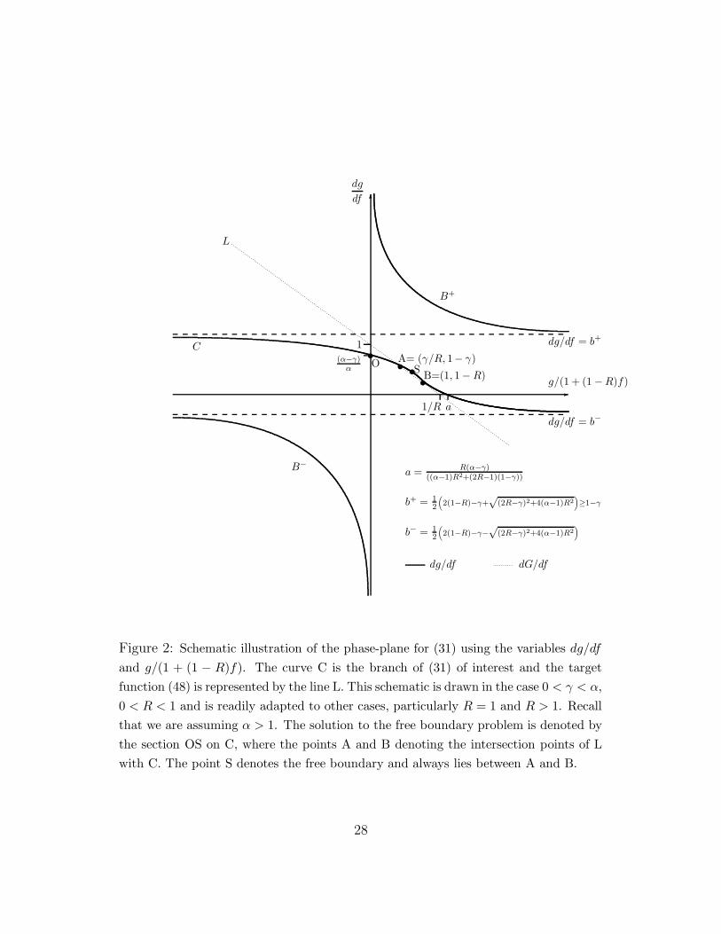
To understand the parameter dependence of the solution, it is informative to

study the shooting problem within a suitable phase-plane. Figure 2 is a diagram

of the phase-plane in the case 0 < γ < R < 1 < α. For convenience we use the

variables dg/df and g/(1+ (1−R)f), which are the first differential invariant (to

within a scaling factor of (1 − R)) and the first invariant respectively. Thus the

study of (31) reduces to an algebraic problem, its curve being shown in Figure

2. As noted earlier, we are interested in the solution branch that passes through

(g, f) = (0, 0), which corresponds to the point O in Figure 2, this branch being

denoted by C. Further, as we are only interested in the range z ∈ (0,∞), we

restrict attention to (1 + (1 − R)f) > 0 and hence the sign of g/(1 + (1 − R)f)

will correspond to that of g. The target function (48) belongs to the family of

solutions todG

df= 1 −

RG

(1 + (1 − R)f), (50)

which corresponds to the straight line L in Figure 2. This line actually represents

the more general one-parameter family of target functions

G = (1 + (1 − R)f) −K(1 + (1 − R)f)−R/(1−R), (51)

for constant K, with our target function corresponding to K = 1. We also note

that (48) has the local behaviour

G = f −R

2f 2 +O(f 3) as f → 0,

which should be compared to the behaviour (35) for the solution of (36).

In the phase-plane of Figure 2, the solution of the free boundary problem is the

section of the curve C denoted by OS. Instrumental in establishing such solutions

within this phase-plane are points where the curve C intersects with the line L.

Substitution of (50) into (31) readily yields the roots for g/(1 + (1 − R)f) as

γ/R and 1 (twice). Thus in general there are two distinct intersection points,

denoted in Figure 2 by A and B respectively. We note that B corresponds to

g = 1 + (1 − R)f which is only attained for the target function (48) in the limit

f → +∞. The point A is an intersection point where dg/df and g/(1+(1−R)f)

are the same for both the IVP and the target function. For our target function,

substituting g/(1 + (1 −R)f) = γ/R into (48) gives immediately that

1 + (1 − R)f ∗s =

(

1 −γ

R

)−(1−R)

.

25

This is the solution (gs(f), f ∗s ) noted in Section 3.3 with the smoothest behaviour

(i.e. maximal regularity) at the free boundary, i.e. the function and its derivative

are continuous. However, we note that although OA lies on C and necessarily

g = 0 at O, it does not follow that f = 0 at the point O. If f 6= 0 at the point

O, then such solutions of the IVP will not be relevant as solutions to our free

boundary problem.

The first issue to be determined from the phase-plane representation is the set

of parameter values for which there exists a solution. A necessary condition for

a solution with g positive is that dg/df > 0 at (f = 0, g = 0), or equivalently the

point O lies on the positive y-axis. Secondly, if γ < 0 then A lies above O on the

curve C and solutions S will lie further to the left along C. In this case we will

get a non-degenerate solution to the problem of repurchasing the real asset sold

short, but the optimal solution for an agent who is long the real asset is to sell

immediately. Hence, for a non-trivial solution we must have 0 < γ < α, and it

follows that γmax ≤ α.

From Figure 1(A) we know that the range for any solutions is confined to

f ∗ ∈ (−1/(1−R),∞). Positive and finite solutions for f ∗ exist if the IVP crosses

the target curve for the domain f > 0. Necessarily then we are restricted to the

points S in Figure 2 lying between A and B where the IVP solution lying on C

has greater slope than the target function lying on L. Since both the solution to

the IVP and the target function eventually meet at B, monotonicity of the IVP

solution (which follows since dg/df > 0 for points along OA) then guarantees a

crossing point with the target function. Recall that Figure 2 was drawn in the

case γ < R, which is a necessary restriction for the point A to lie between O and

B.

The phase-plane in Figure 2 is shown in the case 0 < γ < R < 1 < α and for

these parameter values there will always exist a solution, as represented by the

point S. However it is not possible to tell directly from the phase-plane whether

S is distinct from B, or whether the two points coincide. For γ sufficiently small

S will be distinct from B and there will be a finite exercise trigger. However

for γ > γcrit this will no longer be the case. Determining the value of γcrit will

be one of the subjects of the next Section, and here we content ourselves with

determining some simple bounds.

Continue to suppose that R < 1 < α. As γ increases through R then the

relative position of the points A and B changes, and A moves to the right of B. It

is no longer possible for the solution S to lie to the left of B and hence we must

26

have that S and B coincide. This solution is the degenerate one with f ∗ = ∞

and then z∗ = ∞. Hence γcrit ≤ R.

Now consider increasing γ further until γ = αR. For γ > αR the topology of

the phase-plane changes and the intersection point B moves to the branch B+.

For γ > αR there continues to be a solution to (31)-(33) in the co-ordinates dg/df

and g/(1 + (1 − R)f) but this no longer leads via (40) to a solution in terms of

the economic variables f(z), z and z∗. Essentially the asymptotic growth rates

of IVP and the target function are different so that we do not get smooth fit at

infinity. Hence, for R < 1, γmax = αR.

The above analysis considered the case R < 1, but similar deductions can be

made from the corresponding phase-planes in the cases R = 1 and R > 1. When

R = 1 we have a = 1 and the point B= (1, 0) now lies on the horizontal axis

at the crossing points of both C and L. In this case A will lie to the left of B

provided γ < 1. When R = 1 the requirements that γ < α and γ < αR coincide,

so it is not necessary to consider the case γ > αR and we conclude γmax = α and

γcrit ≤ R = 1.

In the case R > 1 we now expect solutions for f ∗ ∈ (−∞, 1/(R− 1)). By the

earlier remarks on the location of the point O we have γmax = α. In Figure 2,

the point B now lies below the horizontal axis. Again, for a solution S to lie to

the left of B, and thus for f ∗ to lie to the below the upper limit on the range of

its possible values, we must have that A lies to the left of B. Hence a necessary

condition for existence of a finite trigger value is γ < R. Since γcrit ≤ γmax by

definition, when R > 1 we have γcrit ≤ min{α,R}.

It is worth commenting that since the line L intersects C in only two places,

this restricts the possibility of multiple solutions for f ∗ and hence z∗. Thus, in

the case α > 1, the free boundary will be unique when it exists.

5 Numerical Results

The shooting problem described in the previous section facilitates an efficient

numerical method to solve the free boundary problem and produce the parameter

plots given below. We specify the parameters α,R and f ∗ and now treat γ as

unknown. The initial-value problem (36) with (32) (or (42) with (43) for R = 1)

could be solved numerically on the interval [f0, f∗] using the two-term expansion

(35) to specify g at the point f = f0 taken to be close to zero. For implementation

27

-

6

g/(1 + (1 − R)f)

dg

df

C

L

B+

B−

(α−γ)α

1

1/R a

.

.

.

.

.

.

.

.

.

.

.

.

.

.

.

.

.

.

.

.

.

.

.

.

.

.

.

.

.

.

.

.

.

.

.

.

.

.

.

.

.

.

.

.

.

.

.

.

.

.

.

.

.

.

.

.

.

.

.

.

.

.

.

.

.

.

.

.

.

.

.

.

.

.

.

.

.

.

.

.

.

.

.

.

.

.

.

.

.

.

.

.

.

.

.

.

.

.

.

.

.

.

.

.

.

.

.

.

.

.

.

.

.

.

.

.

.

.

.

.

.

.

.

.

.

.

.

.

.

.

.

.

.

.

.

.

.

.

.

.

.

.

.

.

.

.

.

.

.

.

.

.

.

.

.

.

.

.

.

.

.

.

.

.

.

.

.

.

.

.

.

.

.

.

tA= (γ/R, 1− γ)

tB=(1, 1− R)

t

OtS

dg/df = b+

dg/df = b−

a =R(α−γ)

((α−1)R2+(2R−1)(1−γ))

b+ = 12

(

2(1−R)−γ+√

(2R−γ)2+4(α−1)R2

)

≥1−γ

b− = 12

(

2(1−R)−γ−√

(2R−γ)2+4(α−1)R2

)

dg/df .......... dG/df

Figure 2: Schematic illustration of the phase-plane for (31) using the variables dg/df

and g/(1 + (1 − R)f). The curve C is the branch of (31) of interest and the target

function (48) is represented by the line L. This schematic is drawn in the case 0 < γ < α,

0 < R < 1 and is readily adapted to other cases, particularly R = 1 and R > 1. Recall

that we are assuming α > 1. The solution to the free boundary problem is denoted by

the section OS on C, where the points A and B denoting the intersection points of L

with C. The point S denotes the free boundary and always lies between A and B.

28

it was actually found more convenient to numerically solve the second order form

of (36) obtained from differentiating (31), namely

g′′ = −(g′2 + (γ − (1 −R))g′ +R(γ − α))(g′ − (1 − R))

(2gg′ + (γ − 2(1 − R))g − Rα(1 + (1 − R)f)), (52)

subject to

at f = 0 g = 0, g′ =α− γ

α,

where ′ denotes d/df . This formulation avoids the delicate cancellations near

f = 0. Next a minimisation is performed to determine the value of γ for which

the solution of the IVP at f = f ∗ is equal to G(f ∗) where the target function G

is given in (48) (or (49) for R = 1). For the simulations produced below, we used

MATLAB solvers ode45 (or ode15s) with tight error tolerances RelTol=10−10,

AbsTol=10−10 for the IVP and fsolve for the minimisation with optimisation

parameter as small as TolFun=10−30.

5.1 Solutions in the canonical variables

5.1.1 The case 0 < R < 1

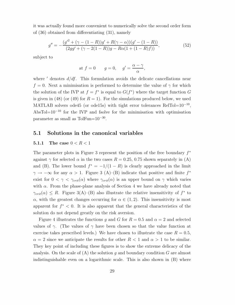
The parameter plots in Figure 3 represent the position of the free boundary f ∗

against γ for selected α in the two cases R = 0.25, 0.75 shown separately in (A)

and (B). The lower bound f ∗ = −1/(1 − R) is clearly approached in the limit

γ → −∞ for any α > 1. Figure 3 (A)–(B) indicate that positive and finite f ∗

exist for 0 < γ < γcrit(α) where γcrit(α) is an upper bound on γ which varies

with α. From the phase-plane analysis of Section 4 we have already noted that

γcrit(α) ≤ R. Figure 3(A)–(B) also illustrate the relative insensitivity of f ∗ to

α, with the greatest changes occurring for α ∈ (1, 2). This insensitivity is most

apparent for f ∗ < 0. It is also apparent that the general characteristics of the

solution do not depend greatly on the risk aversion.

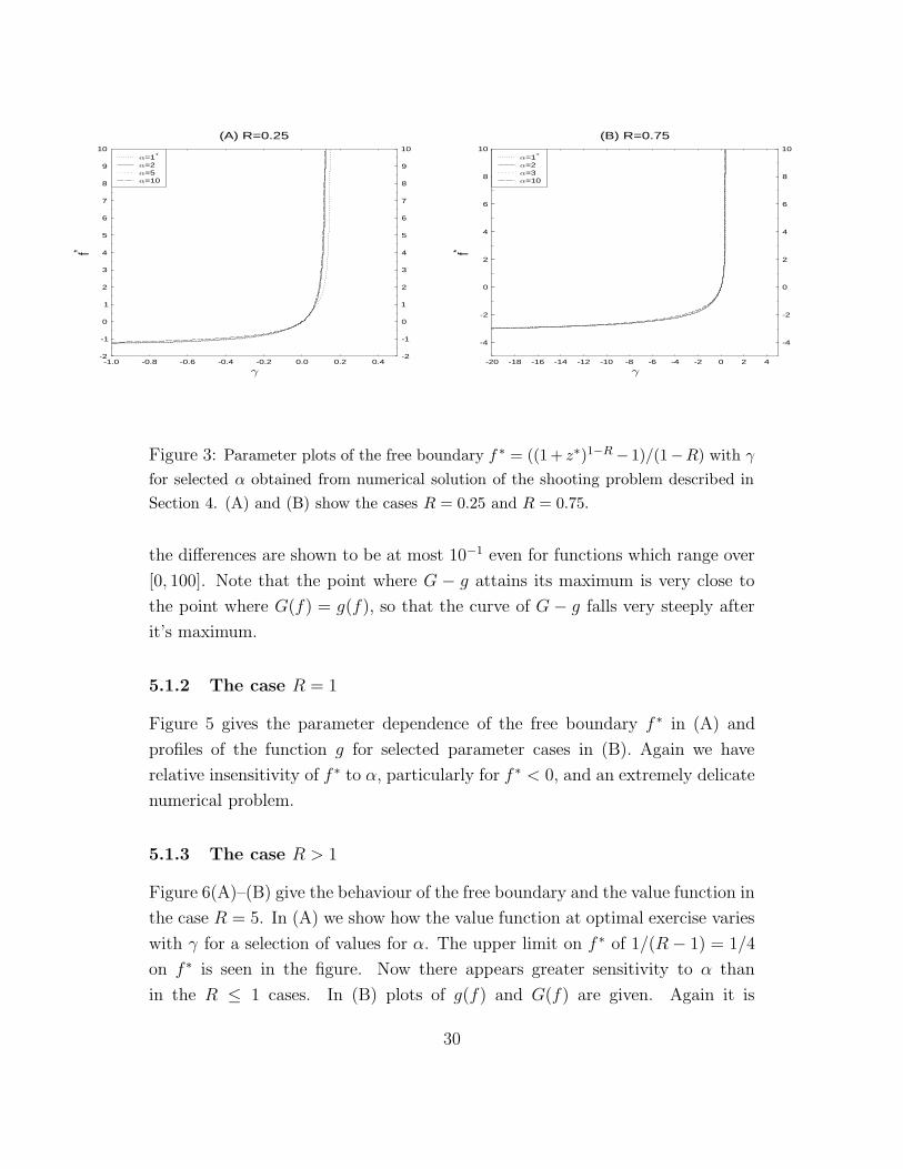
Figure 4 illustrates the functions g and G for R = 0.5 and α = 2 and selected

values of γ. (The values of γ have been chosen so that the value function at

exercise takes prescribed levels.) We have chosen to illustrate the case R = 0.5,

α = 2 since we anticipate the results for other R < 1 and α > 1 to be similar.

They key point of including these figures is to show the extreme delicacy of the

analysis. On the scale of (A) the solution g and boundary condition G are almost

indistinguishable even on a logarithmic scale. This is also shown in (B) where

29

-1.0 -0.8 -0.6 -0.4 -0.2 0.0 0.2 0.4-2

-1

0

1

2

3

4

5

6

7

8

9

10

f*

(A) R=0.25

-2

-1

0

1

2

3

4

5

6

7

8

9

10

=10=5=2=1+

-20 -18 -16 -14 -12 -10 -8 -6 -4 -2 0 2 4

-4

-2

0

2

4

6

8

10

f*

(B) R=0.75

-4

-2

0

2

4

6

8

10

=10=3=2=1+

Figure 3: Parameter plots of the free boundary f ∗ = ((1 + z∗)1−R − 1)/(1−R) with γ

for selected α obtained from numerical solution of the shooting problem described in

Section 4. (A) and (B) show the cases R = 0.25 and R = 0.75.

the differences are shown to be at most 10−1 even for functions which range over

[0, 100]. Note that the point where G − g attains its maximum is very close to

the point where G(f) = g(f), so that the curve of G− g falls very steeply after

it’s maximum.

5.1.2 The case R = 1

Figure 5 gives the parameter dependence of the free boundary f ∗ in (A) and

profiles of the function g for selected parameter cases in (B). Again we have

relative insensitivity of f ∗ to α, particularly for f ∗ < 0, and an extremely delicate

numerical problem.

5.1.3 The case R > 1

Figure 6(A)–(B) give the behaviour of the free boundary and the value function in

the case R = 5. In (A) we show how the value function at optimal exercise varies

with γ for a selection of values for α. The upper limit on f ∗ of 1/(R− 1) = 1/4

on f ∗ is seen in the figure. Now there appears greater sensitivity to α than

in the R ≤ 1 cases. In (B) plots of g(f) and G(f) are given. Again it is

30

10-3 10-2 10-1 100 101 102

f

10-3

10-2

10-1

100

101

102

g(f),

G(f)

(A) R=0.5, =2

10-3

10-2

10-1

100

101

102

f*=100f*=10f*=1f*=0.1G

10-5 10-4 10-3 10-2 10-1 100 101 102

f

10-8

10-7

10-6

10-5

10-4

10-3

10-2

10-1

G(f)-

g(f)

(B) R=0.5, =2

10-8

10-7

10-6

10-5

10-4

10-3

10-2

10-1

f*=100f*=10f*=1f*=0.1

Figure 4: Plots of the numerical solution g and the boundary condition G for R = 0.5,

α = 2 and various values of γ chosen so that the value function at z∗ attains the

levels 0.1, 1, 10, 100. (A) plots both g and G on the same axes, whereas (B) plots the

difference G − g.

-5.0 -4.5 -4.0 -3.5 -3.0 -2.5 -2.0 -1.5 -1.0 -0.5 0.0 0.5 1.0 1.5 2.0-6

-4

-2

0

2

4

6

8

10

12

14

16

18

20

f*

(A) R=1

-6

-4

-2

0

2

4

6

8

10

12

14

16

18

20

=10=5=2=1+

10-3 10-2 10-1 100 101 102

f

10-3

2

5

10-2

2

5

10-1

2

5

100

g(f),

G(f)

(A) R=1, =2

10-3

2

5

10-2

2

5

10-1

2

5

100

f*=100f*=10f*=1f*=0.1G

Figure 5: The logarithmic case R = 1. (A) illustrates the position of the free boundary

as the parameter γ and α vary. (B) gives the solution function g and boundary condition

G plotted as a function of f .

31

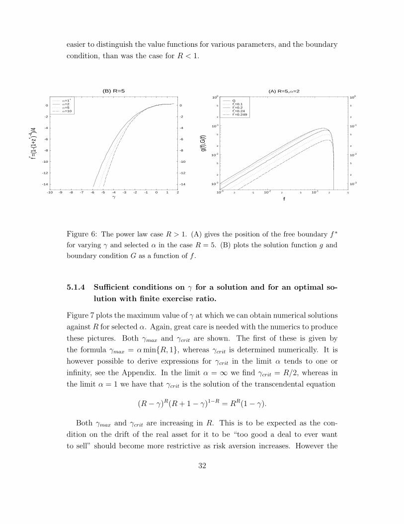
easier to distinguish the value functions for various parameters, and the boundary

condition, than was the case for R < 1.

-10 -9 -8 -7 -6 -5 -4 -3 -2 -1 0 1 2

-14

-12

-10

-8

-6

-4

-2

0

f* =(1-

(1+z

* )-4)/4

(B) R=5

-14

-12

-10

-8

-6

-4

-2

0

=10=5=2=1+

10-32 5 10-2

2 5 10-12 5

f

10-3

2

5

10-2

2

5

10-1

2

5

100

g(f),

G(f)

(A) R=5, =2

10-3

2

5

10-2

2

5

10-1

2

5

100

f*=0.249f*=0.24f*=0.2f*=0.1G

Figure 6: The power law case R > 1. (A) gives the position of the free boundary f ∗

for varying γ and selected α in the case R = 5. (B) plots the solution function g and

boundary condition G as a function of f .

5.1.4 Sufficient conditions on γ for a solution and for an optimal so-

lution with finite exercise ratio.

Figure 7 plots the maximum value of γ at which we can obtain numerical solutions

against R for selected α. Again, great care is needed with the numerics to produce

these pictures. Both γmax and γcrit are shown. The first of these is given by

the formula γmax = αmin{R, 1}, whereas γcrit is determined numerically. It is

however possible to derive expressions for γcrit in the limit α tends to one or

infinity, see the Appendix. In the limit α = ∞ we find γcrit = R/2, whereas in

the limit α = 1 we have that γcrit is the solution of the transcendental equation

(R− γ)R(R + 1 − γ)1−R = RR(1 − γ).

Both γmax and γcrit are increasing in R. This is to be expected as the con-

dition on the drift of the real asset for it to be “too good a deal to ever want

to sell” should become more restrictive as risk aversion increases. However the

32

dependence on α is less clear. For small R it appears that γcrit(α) is decreasing in

α, but for large R the relationship is reversed. The limit limR↑∞ γcrit(α,R) → α

can easily be seen in Figure 7.

10-22 5 10-1

2 5 1002 5 101

2

R

10-2

2

5

10-1

2

5

100

2

5

101

2

5

102

max

,crit

10-2

2

5

10-1

2

5

100

2

5

101

2

5

102

=10=5=2=1+

=10=5=2=1

max crit=R/2

Figure 7: The largest value of γ for which we can obtain solutions, plotted against R

for selected α. There are two lines shown for each value of α. The piecewise linear curve

shows γmax, the maximum value of γ for which the value function exists. (For larger

values of γ the agent would not agree to sell the real asset at any price.) The smooth

curve shows γcrit, the critical value of γ at which the free boundary first becomes

infinite. Note that γcrit ≤ min{α,R}. Also shown is the line γ = R/2 which is the

critical value of γ in the limit α ↑ ∞.

33

6 Interpretation of the results in terms of eco-

nomic variables

Here we present the results in more economically meaningful variables (H(z), z, z∗)

and the utility indifference price described in Section 2.5, rather than the canon-

ical variables which were used in the previous section.

We use representative parameter values λ = 0.15, σ = 0.3 and ξ ∈ {0.1, 0.15, 0.2}.

Correlation can range over (−1, 1) though we generally present results for posi-

tive ρ, and the risk aversion parameter R is varied over a wide range. For Figure

9 we use the realistic value of R = 5.

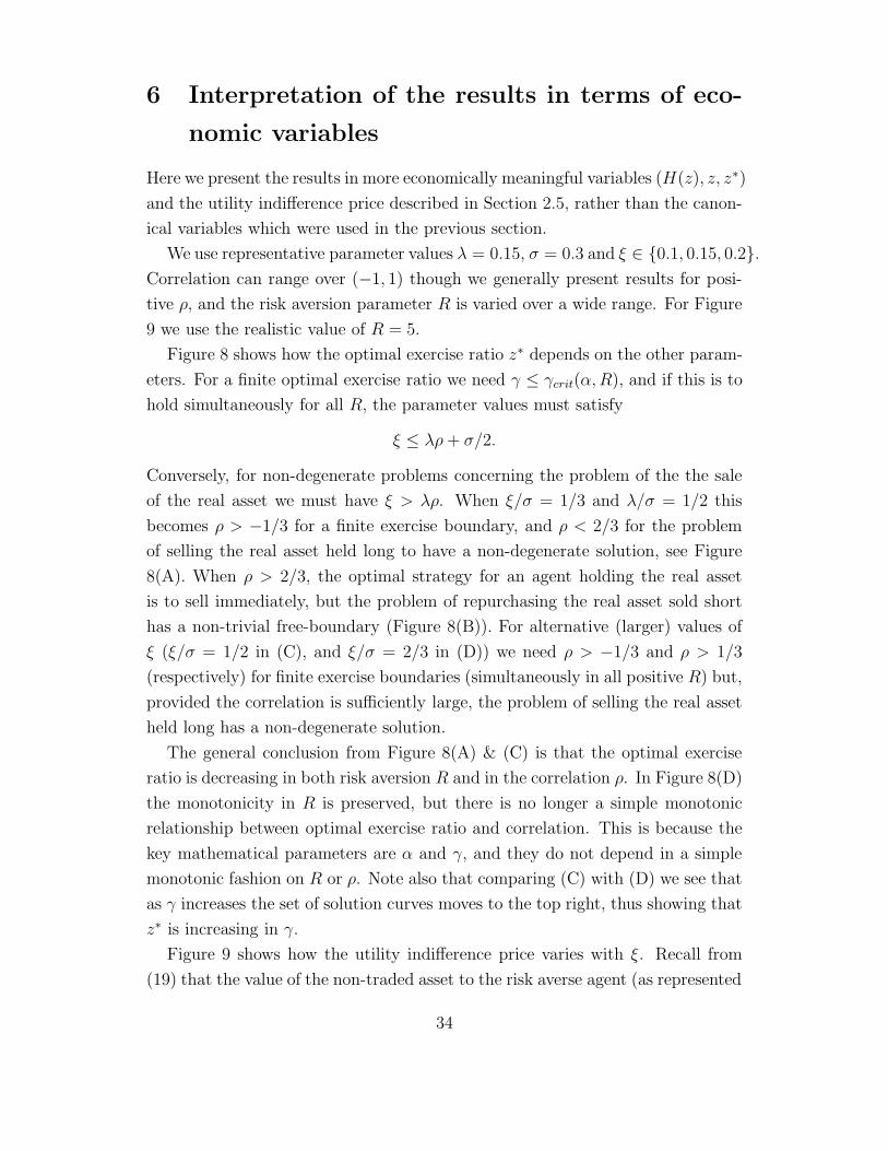
Figure 8 shows how the optimal exercise ratio z∗ depends on the other param-

eters. For a finite optimal exercise ratio we need γ ≤ γcrit(α,R), and if this is to

hold simultaneously for all R, the parameter values must satisfy

ξ ≤ λρ+ σ/2.

Conversely, for non-degenerate problems concerning the problem of the the sale

of the real asset we must have ξ > λρ. When ξ/σ = 1/3 and λ/σ = 1/2 this

becomes ρ > −1/3 for a finite exercise boundary, and ρ < 2/3 for the problem

of selling the real asset held long to have a non-degenerate solution, see Figure

8(A). When ρ > 2/3, the optimal strategy for an agent holding the real asset

is to sell immediately, but the problem of repurchasing the real asset sold short

has a non-trivial free-boundary (Figure 8(B)). For alternative (larger) values of

ξ (ξ/σ = 1/2 in (C), and ξ/σ = 2/3 in (D)) we need ρ > −1/3 and ρ > 1/3

(respectively) for finite exercise boundaries (simultaneously in all positive R) but,

provided the correlation is sufficiently large, the problem of selling the real asset

held long has a non-degenerate solution.

The general conclusion from Figure 8(A) & (C) is that the optimal exercise

ratio is decreasing in both risk aversion R and in the correlation ρ. In Figure 8(D)

the monotonicity in R is preserved, but there is no longer a simple monotonic

relationship between optimal exercise ratio and correlation. This is because the

key mathematical parameters are α and γ, and they do not depend in a simple

monotonic fashion on R or ρ. Note also that comparing (C) with (D) we see that

as γ increases the set of solution curves moves to the top right, thus showing that

z∗ is increasing in γ.

Figure 9 shows how the utility indifference price varies with ξ. Recall from

(19) that the value of the non-traded asset to the risk averse agent (as represented

34

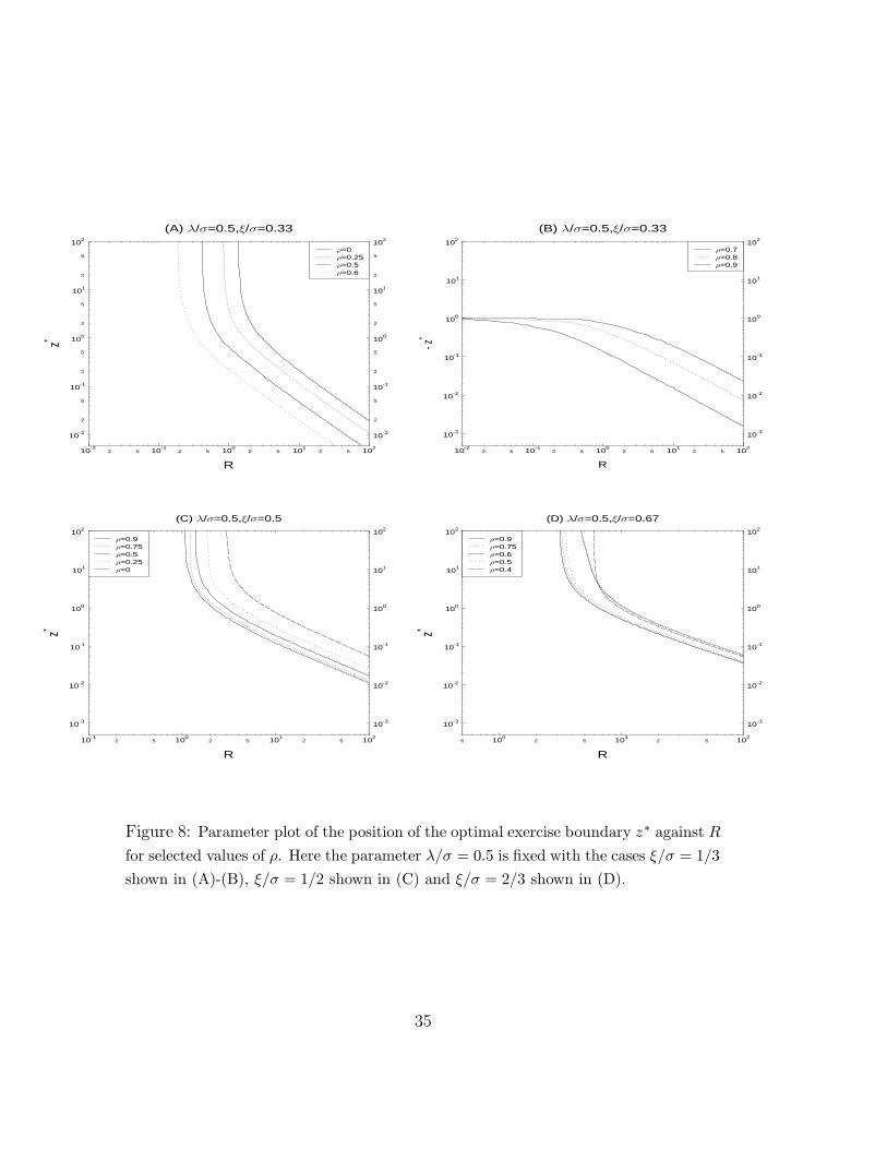
10-22 5 10-1

2 5 1002 5 101

2 5 102

R

10-2

2

5

10-1

2

5

100

2

5

101

2

5

102

z*

(A) / =0.5, / =0.33

10-2

2

5

10-1

2

5

100

2

5

101

2

5

102

=0.6=0.5=0.25=0

10-22 5 10-1

2 5 1002 5 101

2 5 102

R

10-3

10-2

10-1

100

101

102

-z*

(B) / =0.5, / =0.33

10-3

10-2

10-1

100

101

102

=0.9=0.8=0.7

10-12 5 100

2 5 1012 5 102

R

10-3

10-2

10-1

100

101

102

z*

(C) / =0.5, / =0.5

10-3

10-2

10-1

100

101

102

=0=0.25=0.5=0.75=0.9

5 1002 5 101

2 5 102

R

10-3

10-2

10-1

100

101

102

z*

(D) / =0.5, / =0.67

10-3

10-2

10-1

100

101

102

=0.4=0.5=0.6=0.75=0.9

Figure 8: Parameter plot of the position of the optimal exercise boundary z∗ against R

for selected values of ρ. Here the parameter λ/σ = 0.5 is fixed with the cases ξ/σ = 1/3

shown in (A)-(B), ξ/σ = 1/2 shown in (C) and ξ/σ = 2/3 shown in (D).

35

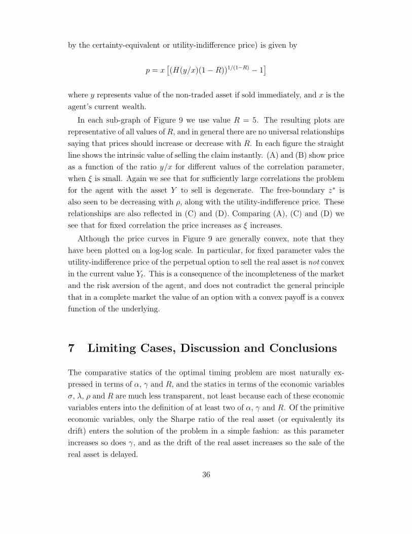
by the certainty-equivalent or utility-indifference price) is given by

p = x[

(H(y/x)(1− R))1/(1−R) − 1]

where y represents value of the non-traded asset if sold immediately, and x is the

agent’s current wealth.

In each sub-graph of Figure 9 we use value R = 5. The resulting plots are

representative of all values ofR, and in general there are no universal relationships

saying that prices should increase or decrease with R. In each figure the straight

line shows the intrinsic value of selling the claim instantly. (A) and (B) show price

as a function of the ratio y/x for different values of the correlation parameter,

when ξ is small. Again we see that for sufficiently large correlations the problem

for the agent with the asset Y to sell is degenerate. The free-boundary z∗ is

also seen to be decreasing with ρ, along with the utility-indifference price. These

relationships are also reflected in (C) and (D). Comparing (A), (C) and (D) we

see that for fixed correlation the price increases as ξ increases.

Although the price curves in Figure 9 are generally convex, note that they

have been plotted on a log-log scale. In particular, for fixed parameter vales the

utility-indifference price of the perpetual option to sell the real asset is not convex

in the current value Yt. This is a consequence of the incompleteness of the market

and the risk aversion of the agent, and does not contradict the general principle

that in a complete market the value of an option with a convex payoff is a convex

function of the underlying.

7 Limiting Cases, Discussion and Conclusions

The comparative statics of the optimal timing problem are most naturally ex-

pressed in terms of α, γ and R, and the statics in terms of the economic variables

σ, λ, ρ and R are much less transparent, not least because each of these economic

variables enters into the definition of at least two of α, γ and R. Of the primitive

economic variables, only the Sharpe ratio of the real asset (or equivalently its

drift) enters the solution of the problem in a simple fashion: as this parameter

increases so does γ, and as the drift of the real asset increases so the sale of the

real asset is delayed.

36

10-5 10-4 10-3 10-2 10-1 100

z

10-3

2

5

10-2

2

5

10-1

2

5

100

2

(H(z

)(1-R

))(1/(1

-R)) -1

(A) R=5, / =0.5, / =0.33

10-3

2

5

10-2

2

5

10-1

2

5

100

2

=0.6=0.5=0.25=0

10-42 5 10-3

2 5 10-22 5 10-1

2 5 1002

-z

10-3

2

5

10-2

2

5

10-1

2

5

100

2

5

101

-((H

(z)(1

-R))(1

/(1-R

)) -1)

(B) R=5, / =0.5, / =0.33

10-3

2

5

10-2

2

5

10-1

2

5

100

2

5

101

=0.9=0.8=0.7

10-8 10-7 10-6 10-5 10-4 10-3 10-2 10-1 100 101

z

10-3

2

5

10-2

2

5

10-1

2

5

100

2

5

101

(H(z

)(1-R

))(1/(1

-R)) -1

(C) R=5, / =0.5, / =0.5

10-3

2

5

10-2

2

5

10-1

2

5

100

2

5

101

=0.9=0.75=0.5=0.25=0

10-8 10-7 10-6 10-5 10-4 10-3 10-2 10-1 100 101

z

10-3

2

5

10-2

2

5

10-1

2

5

100

2

5

101

(H(z

)(1-R

))(1/(1

-R)) -1

(D) R=5, / =0.5, / =0.67

10-3

2

5

10-2

2

5

10-1

2

5

100

2

5

101

=0.9=0.75=0.5=0.45

Figure 9: Plots of the price function(

(H(z)(1 − R))1/(1−R) − 1)

against z for selected

parameter cases of those illustrated in Figure 8. The parameter λ/σ = 0.5 is fixed

throughout. The case ξ/σ = 1/3 is shown in (A) and (B) for selected ρ. The cases

ξ/σ = 1/2 and ξ/σ = 2/3 are given in (C) and (D) respectively. In each case the

coefficient of risk aversion is R = 5.

37

7.1 Limiting cases

7.1.1 The limit of zero risk aversion: R ↓ 0.

If we consider the limit as risk aversion decreases to zero then we find that there

is no non-degenerate solution. If γ > 0 (or equivalently ξ > λρ) then there is no

finite ratio at which exercise is optimal. Conversely, if γ ≤ 0 then it is always

optimal to sell the real asset instantly. In this case, if the real asset has positive

drift under the (Follmer-Schweizer [5]) minimal martingale measure, then the

sale should be delayed, otherwise the real asset should be sold instantly.

7.1.2 The limit of infinite risk aversion: R ↑ ∞.

If γ < 0 it is always optimal to sell instantly. Otherwise the key criterion is the

necessity of γ < α (recall Figure 7 and the limit R ↑ ∞) for the existence of

a non-degenerate solution. For 0 < ξ < λρ + σ/2 there is a finite investment

trigger for the real asset/trading wealth ratio, otherwise the investment trigger

is infinite. Note that this conclusion mirrors the results of Henderson [7] (who

considers perpetual call options with non-zero strikes) under exponential utility,

and reflects the fact that exponential utility can be considered as the limit as risk

aversion increases to infinity of power-law utility.

7.1.3 The limit of perfect correlation |ρ| ↑ 1.

This is the complete-market limit in which the real asset is spanned by the market.

The behaviour of the parameters α and γ can be determined from (17).

There are special cases depending on whether ξ = ±λ or otherwise, and λ =

σR or otherwise, and different cases for R < 1 and R > 1. In each case the form

of the optimal solution depends on the relative values of γ and each of γcrit(α,R)

and γmax(α,R). There are many cases to consider, but in the typical case both α

and γ grow linearly with (1 − ρ)−1 and it is necessary to compare the constants

in the growth rates.

7.2 General Remarks

In this article we have considered the optimal behaviour of an agent who has the

right to liquidate an investment, or to sell a real asset. Provided this investment

has a positive Sharpe ratio (ξ > 0) the agent can get a better expected return

38

on the market than from a passive investment in the bank account. However,

maintaining the investment in the real asset imposes an opportunity cost associ-

ated with the ability of the agent to invest part of her wealth in the best market

investments. Although she may benefit from a diversification effect, the agent

who can trade in a financial market will only continue to invest in the real asset

if ξ > λρ.

However, even in these cases, continuing to hold the real asset exposes the

agent to idiosyncratic (non-hedgeable) risk. Even if the return on the real asset is

sufficient to justify some investment, if the proportion of her wealth that the agent

has in the real asset is sufficiently large, then the risk-averse agent may choose

to sell. This effect occurs because the real asset is assumed to be indivisible, and

the exposure to risk can only be partially hedged using market instruments.

Thus, for γ > 0 there may be a finite optimal exercise ratio, and when the value

of the real asset relative to the agent’s wealth first exceeds this ratio, the agent

should sell the real asset. However, as γ increases this optimal ratio increases,

until for some value γcrit ≤ min{α,R} this ratio becomes infinite. At this point

the agent trades in such a way that her wealth may become zero, and the first

time this happens she must sell the real asset. For sufficiently large returns on

the indivisible, real asset the agent will never choose to sell the asset, as the

expected future returns always more than compensate for the unhedgeable risk

which remains from holding the real asset.

The above generic remarks show our conclusions have a natural intuitive in-

terpretation in terms of the economics of the problem. However, perhaps the key

contribution of this paper is to show how to formulate and to characterise the

solution of the associated optimal stopping problem. One of the key quantities

of interest is the free boundary at which exercise takes place. Free boundary

problems are generally very difficult, (for instance the optimal exercise boundary

of a finite horizon American put option) but in this case it is possible to repre-

sent the free-boundary as the solution of a transcendental equation. Determining

when this equation has a non-degenerate solution brings insight to the questions

of determining when the optimal exercise behaviour is non-degenerate and is the

first step towards the pricing of the real asset in the incomplete market.

39

References

[1] M.H.A. Davis and T. Zariphopoulou. American options and transaction fees.

In Mathematical Finance IMA Volumes in Mathematics and its Applications.

Springer-Verlag, 1995.

[2] A.K. Dixit and R.S. Pindyck. Investment under uncertainty. Princeton

University Press, 1994.

[3] C.M. Elliott and J. Ockendon. Weak and variational methods for free and

moving boundary problems. Pitman, London, 1982.

[4] J. D. Evans, V. Henderson, and D.G. Hobson. The curious incident of the

investment in the market. Technical report, Princeton University, 2005.

[5] H. Follmer and M. Schweizer. Hedging of contingent claims under incomplete

information. In M.H.A. Davis and R.J. Elliott, editors, Applied Stochastic

Analysis, pages 389–414. Gordon and Breach, London, 1990.

[6] V. Henderson. Valuation of claims on non-traded assets using utility maxi-

mization. Mathematical Finance, 12(4):351–373, 2002.

[7] V. Henderson. Valuing the option to invest in an incomplete market. Tech-

nical report, Princeton University, 2004.

[8] V. Henderson and D. Hobson. Real options with constant relative risk aver-

sion. Journal of Economic Dynamics and Control, 27:329–355, 2002.

[9] V. Henderson and D. Hobson. Utility indifference pricing - an overview. In

R. Carmona, editor, Indifference Pricing. Princeton University Press, Prince-

ton, NJ, 2005.

[10] S. Hodges and A. Neuberger. Optimal replication of contingent claims under

transactions costs. Review of Futures Markets, 8:222–239, 1989.

[11] F. Hubalek and W. Schachermayer. Optimizing expected utility of dividend

payments for a brownian risk process and a peculiar nonlinear ode. Insur-

ance: Mathematics and Economics, 34:193–225, 2004.

[12] T. Johnson, K. Watson, and M. Zervos. An optimal stopping problem with

applications to the timing of investment decisions. Technical report, King’s

College, London, 2004.

40

[13] I. Karatzas and S.G. Kou. Hedging american contingent claims with con-

strained portfolios. Finance and Stochastics, 2:215–258, 1998.

[14] I. Karatzas and H. Wang. Utiilty maximisation with discretionary stopping.

SIAM J. Control Optim., 39:306–329, 2000.

[15] R. McDonald and D.R. Siegel. The value of waiting to invest. Quarterly

Journal of Economics, 101:707–727, 1986.

[16] H.P. McKean. A free boundary problem for the heat equation arising from a

problem in mathematical economics. Industrial Management Review, 6:32–

39, 1965.

[17] J. Miao and N. Wang. Investment, hedging and consumption smoothing.

Technical report, Boston University, 2005.

[18] M. Musiela and T. Zariphopoulou. An example of indifference prices under

exponential preferences. Finance and Stochastics, 8(2):229–239, 2004.

[19] A. Oberman and T. Zariphopoulou. Pricing early exercise contracts in in-

complete markets. Computational Management Science, 1:75–107, 2003.

[20] J. Ockendon, S. Howison, A. Lacey, and A. Movchan. Applied Partial Dif-

ferential Equations. Oxford University Press, Oxford, 1999.

[21] J.E. Smith and R.F. Nau. Valuing risky projects: option pricing theory and

analysis. Management Science, 41(5):795–816, 1995.

[22] N. Touzi. Stochastic control problems, viscosity solutions and application to

finance. Technical report, Special Research Semester on Financial Markets,

Pisa, 2002.

[23] A. Vollert. A Stochastic Control Framework for Real Options. Birkhauser,

Boston, 2003.

[24] P. Wilmott, S.D. Howison, and J.N. Dewynne. The Mathematics of Financial

Derivatives: A Student Introduction. CUP, New York, 1995.

[25] T. Zariphopoulou. A solution approach to valuation with unhedgeable risks.

Finance and Stochastics, 4:61–82, 2001.

41

A Limiting values of α.

A.1 The large α limit

We may explore the limiting case of the solution to (22)-(23) when α becomes

large and γ = O(1). This limit is regular and may be analysed by formally

writing

α =1

ε,

and considering the limit ε→ 0. Posing the expansion

g = g0 + εg1 +O(ε2),

(31) (or equivalently (36)), (32) and (33) give the leading order problem

dg0

df= 1 − R

g0

(1 + (1 −R)f)(53)

at f = 0 g0 = 0, (54)

at f = f ∗ g0 = (1 + (1 −R)f ∗) − (1 + (1 − R)f ∗)−R/(1−R) , (55)

and the first order problem

R(1 + (1 −R)f)dg1

df+R2g1 = g0

(

dg0

df

)2

+ (γ − 2(1 − R))g0dg0

df(56)

+g0(R2 + (2R− 1)(γ − 1)) − Rγ(1 + (1 −R)f)

at f = 0 g1 = 0, (57)

at f = f ∗ g1 = 0. (58)

The leading order problem has the exact solution

g0 = (1 + (1 − R)f) − (1 + (1 − R)f)−R/(1−R)

which we note satisfies (55) identically and thus we must proceed to the next

order to determine f ∗. Again this is an indication of why the numerical problem

is so delicate, particularly as the results of Section 5 indicate that this α-large

limit is actually attained at relatively small values of α ie. for α > 2 we are

effectively in the large-α regime. The first order problem (56) and (57) has the

solution

g1 =R

2(1+(1−R)f)R/(R−1) (1−(1+(1−R)f)1/(R−1))

(

1 −2γ

R− (1 + (1 −R)f)1/(R−1)

)

,

(59)

42

which is most easily derived in transformed variables w = (1+(1−R)f), v = g1/w.

Imposing (55) then gives

f ∗ =1

(1 − R)

(

(

1 −2γ

R

)R−1

− 1

)

(60)

for the free-boundary. We note that γ = R/2 gives the critical values of f ∗ = +∞

for R ≤ 1 and f ∗ = 1/(R− 1) for R > 1. Thus, limα↑∞ γcrit = R/2.

In the logarithmic case R = 1, the above expressions simplify to

g0 = 1 − e−f , g1 =1

2e−f (1 − e−f ) (1 − 2γ − e−f ), f ∗ = − ln(1 − 2γ),

with f ∗ = +∞ when γ = 1/2 and limα↑∞ γcrit = 1/2.

A.2 The case α = 1

This case is the subject of the companion paper [4]. However we provide a brief

discussion of the derivation of the form of the transcendental equation for γcrit.

In the case α = 1, the analysis of Section 3 both simplifies and changes. In

this case, we have

a(v;R) =

{

2(1 − γ)v, if v ≤ R/(2R− γ),

2R + 2(1 − 2R)v, if v > R/(2R− γ),

and introducing

fc =R

(R− γ)(R + 1 − γ),

(38) becomes

g = (1 − γ)f, if f ≤ fc , (61)

with f ∗ ≤ fc determined by the transcendental equation

(1 − γ)f ∗ = (1 + (1 − R)f ∗) − (1 + (1 −R)f ∗)−R/(1−R). (62)

However, if f > fc then (38) becomes

∫ g/(1+(1−R)f)

R/(2R−γ)

v dv

(1 − v)(R+ (1 − R)v)=

1

(1 −R)ln

(

(1 + (1 −R)f)

(1 + (1 −R)fc)

)

. (63)

This expression may be evaluated, and using (62) it is possible to obtain an

explicit expression for f ∗ in terms of R and γ.

43

As f ∗ → +∞ for R ≤ 1 or f ∗ → 1/(R − 1) for R > 1 this expression has

limiting behaviour

(R− γ)R(R + 1 − γ)1−R = RR(1 − γ),

the solution of which, for fixed R, places an upper bound on the set of γ for which

the optimal sale problem has a finite trigger ratio.

44