Optimal Taylor–Couette flow: radius ratio dependence

arX

iv:1

304.

6331

v2 [

phys

ics.

flu-

dyn]

29

Oct

201

3

Under consideration for publication in J. Fluid Mech. 1

Optimal Taylor-Couette flow:radius ratio dependence

RODOLFO OSTILLA M O NICO1,SANDER G. HUISMAN1,

T IM J. G. JANNINK1, DENNIS P. M. VAN GILS1,ROBERTO VERZICCO2,1,

S IEGFRIED GROSSMANN3, CHAO SUN1,AND DETLEF LOHSE1

1Physics of Fluids, Mesa+ Institute, University of Twente, P.O. Box 217, 7500 AE Enschede,The Netherlands

2Dipartimento di Ingegneria Meccanica, University of Rome “Tor Vergata”, Via del Politecnico1, Roma 00133, Italy

3Department of Physics, University of Marburg, Renthof 6, D-35032 Marburg, Germany

(Received 30 October 2013)

Taylor–Couette flow with independently rotating inner (i) & outer (o) cylinders is ex-plored numerically and experimentally to determine the effects of the radius ratio η on thesystem response. Numerical simulations reach Reynolds numbers of up to Rei = 9.5 · 103and Reo = 5 · 103, corresponding to Taylor numbers of up to Ta = 108 for four differentradius ratios η = ri/ro between 0.5 and 0.909. The experiments, performed in the TwenteTurbulent Taylor–Couette (T 3C) setup, reach Reynolds numbers of up to Rei = 2 · 106and Reo = 1.5 ·106, corresponding to Ta = 5 · 1012 for η = 0.714−0.909. Effective scalinglaws for the torque Jω(Ta) are found, which for sufficiently large driving Ta are indepen-dent of the radius ratio η. As previously reported for η = 0.714, optimum transport ata non–zero Rossby number Ro = ri|ωi − ωo|/[2(ro − ri)ωo] is found in both experimentsand numerics. Roopt is found to depend on the radius ratio and the driving of the system.At a driving in the range between Ta ∼ 3 · 108 and Ta ∼ 1010, Roopt saturates to anasymptotic η-dependent value. Theoretical predictions for the asymptotic value of Rooptare compared to the experimental results, and found to differ notably. Furthermore, thelocal angular velocity profiles from experiments and numerics are compared, and a linkbetween a flat bulk profile and optimum transport for all radius ratios is reported.

Key words:

1. Introduction

Taylor-Couette (TC) flow consists of the flow between two coaxial cylinders which areindependently rotating. A schematic drawing of the system can be seen in Fig. 1. Therotation difference between the cylinder shears the flow thus driving the system. Thisrotation difference has been traditionally expressed by two Reynolds numbers, the innercylinder Rei = riωid/ν, and the outer cylinder Reo = roωod/ν Reynolds numbers, whereri and ro are the radii of the inner and outer cylinder, respectively, ωi and ωo the inner andouter cylinder angular velocity, d = ro − ri the gap width, and ν the kinematic viscosity.

2 R. Ostilla Monico and others

L

ri

ro

o

i

Figure 1: Schematic of the Taylor-Couette system. The system consists of two coaxialcylinders, which have an inner cylinder radius of ri and an outer cylinder radius of ro.Both cylinders are of length L. The inner cylinder rotates with an angular velocity ωi

and the outer cylinder rotates with an angular velocity of ωo.

The geometry of TC is characterized by two nondimensional parameters, namely theradius ratio η = ri/ro and the aspect ratio Γ = L/d.Instead of taking Rei and Reo, the driving in TC can alternatively be characterized

by the Taylor Ta and the rotation rate, also called the Rossby Ro number. The Taylornumber can be seen as the non-dimensional forcing (the differential rotation) of thesystem defined as Ta = σ(ro − ri)

2(ro + ri)2(ωo − ωi)

2/(4ν2), or

Ta = (r6ad2/r2or

2

i ν2)(ωo − ωi)

2. (1.1)

Here σ = r4a/r4g with ra = (ro + ri)/2 the arithmetic and rg =

√rori the geometric mean

radii. The Rossby number is defined as:

Ro =|ωi − ωo|ri

2ωod, (1.2)

and can be seen as a measure of the rotation of the system as a whole. Ro < 0 correspondsto counterrotating cylinders, and Ro > 0 to corotating cylinders.TC is among the most investigated systems in fluid mechanics, mainly owing to its

simplicity as an experimental model for shear flows. TC is in addition a closed system, soglobal balances which relate the angular velocity transport to the energy dissipation canbe obtained. Specifically, in Eckhardt, Grossmann & Lohse (2007) (from now on referredto as EGL 2007), an exact relationship between the global parameters and the volumeaveraged energy dissipation rate was derived. This relationship has an analogous form tothe one which can be obtained for Rayleigh-Benard (RB) flow, i.e. a flow in which heatis transported from a hot bottom plate to a cold top plate.TC and RB flow have been extensively used to explore new concepts in fluid mechan-

Optimal Taylor-Couette flow: Radius ratio dependence 3

ics. Instabilities (Swinney & Gollub 1981; Pfister & Rehberg 1981; Pfister et al. 1988;Chandrasekhar 1981; Drazin & Reid 1981; Busse 1967), nonlinear dynamics and chaos(Lorenz 1963; Ahlers 1974; Behringer 1985; Dominguez-Lerma et al. 1986; Strogatz 1994),pattern formation (Andereck et al. 1986; Cross & Hohenberg 1993; Bodenschatz et al.

2000), and turbulence (Siggia 1994; Grossmann & Lohse 2000; Kadanoff 2001; Lathrop et al.

1992b; Ahlers et al. 2009; Lohse & Xia 2010) have been studied in both TC and RB andboth numerically and experimentally. The main reasons behind the popularity of thesesystems are, in addition to the fact that they are closed systems, as mentioned previously,their simplicity due to the high amount of symmetries present. It is also worth notingthat plane Couette flow is the limiting case of TC when the radius ratio η = 1.Experimental investigations of TC have a long history, dating back to the initial work

in the end of the 1800s by Couette (1890) in France, who concentrated on outer cylinderrotation and developed the viscometer and Mallock (1896) in the UK, who also rotatedthe inner cylinder and found indications of turbulence. Later work by Wendt (1933)and Taylor (1936), greatly expanded on the system, the former measuring torques andvelocities for several radius and rotation ratios in the turbulent case, and the latter beingthe first to mathematically describe the cells which form if the flow is linearly unstable.The subject can be traced back even further to Stokes, and even Newton. For a broaderhistorical context, we refer the reader to Donnelly (1991).Experimental work continued during the years (Smith & Townsend 1982; Andereck et al.

1986; Tong et al. 1990; Lathrop et al. 1992b,a; Lewis & Swinney 1999; van Gils et al.2011a,b; Paoletti & Lathrop 2011; Huisman et al. 2012b) at low and high Ta numbers fordifferent ratios of the rotation frequencies a = −ωo/ωi. a is positive for counter–rotationand negative for co–rotation. −a ≡ µ, another measure used for the ratio of rotationfrequencies. This work has been complemented by numerical simulations, not only inthe regime of pure inner cylinder rotation (Fasel & Booz 1984; Coughlin & Marcus 1996;Dong 2007, 2008; Pirro & Quadrio 2008), but also for eigenvalue study (Gebhardt & Grossmann1993), and counter-rotation at fixed a (Dong 2008). Recently (Brauckmann & Eckhardt2013a; Ostilla et al. 2013), simulations have also explored the effect of the outer cylinderrotation on the system at large Reynolds numbers.The recent experiments (van Gils et al. 2011a,b; Paoletti & Lathrop 2011; Merbold et al.

2013) and simulations (Brauckmann & Eckhardt 2013a; Ostilla et al. 2013) have shownthat at fixed Ta an optimal angular momentum transport is obtained at non-zero aopt,and that the location of this maximum aopt varies with Ta. However, both experi-ments and simulations have been restricted to two radius ratios, namely η = 0.5 andη = 0.714. The same radius ratios were also used for studies carried out on scalinglaws of the torque and the “wind” of turbulence at highly turbulent Taylor numbers(Lewis & Swinney 1999; Paoletti & Lathrop 2011; van Gils et al. 2011b; Huisman et al.

2012b; Merbold et al. 2013). Up to now, it is not clear how the radius ratio affects thescaling laws of the system response or the recently found phenomena of optimal transportas a function of Ta.Two suggestions were made to account for the radius ratio dependence of optimal

transport. Van Gils et. al (2011b) wondered whether the optimal transport in generallies in or at least close to the Voronoi boundary (meaning a line of equal distance) of theEsser-Grossmann stability lines (Esser & Grossmann 1996) in the (Reo, Rei) phase spaceas it does for η = 0.714. However, this bisector value does not give the correct optimaltransport for η = 0.5 (Merbold et al. 2013; Brauckmann & Eckhardt 2013b). ThereforeBrauckmann & Eckhardt (2013a) proposed a dynamic extension of the Esser-Grossmanninstability theory. This model correctly gives the observed optimal transport (withinexperimental error bars) between η = 0.5 and η = 0.714 for three experimental data sets

4 R. Ostilla Monico and others

(Wendt 1933; Paoletti & Lathrop 2011; van Gils et al. 2011b) and one numerical data set(Brauckmann & Eckhardt 2013b), but it is not clear how it performs outside the η-range[0.5, 0.714].In this paper, we study the following questions: how does the radius ratio η affect the

flow? How are the scaling laws of the angular momentum transport affected? What is therole of the geometric parameter called pseudo-Prandtl number σ introduced in EGL2007?Can the effect of the radius ratio be interpreted as a kind of non-Oberbeck-Boussinesqeffect, analogous to this effect in Rayleigh-Benard flow? Finally, are the predictionsand insights of van Gils et al. (2011b), Ostilla et al. (2013) and Brauckmann & Eckhardt(2013b) on the optimal transport also valid for other values of η?In order to answer these questions, both direct numerical simulations (DNS) and

experiments have been undertaken. Numerical simulations, with periodic axial bound-ary conditions, have been performed using the finite–difference code previously used inOstilla et al. (2013). In these simulations, three more values of η have been investigated:one in which the gap is larger (η = 0.5), and two in which the gap is smaller (η = 0.833and 0.909). With the previous simulations from Ostilla et al. (2013) at η = 0.714, a totalof four radius ratios has been analyzed.In both experiments and numerics, only one aspect ratio Γ has been studied for every

radius ratio. Since the work of Benjamin (1978) it is known that multiple flow stateswith a different amount of vortex pairs can coexist in TC for the same non-dimensionalflow parameters. However, with increased driving, the bifurcations become less importantand many branches do not survive. Indeed, Lewis & Swinney (1999) found that for pureinner cylinder rotation only one branch with 8 vortices (for Γ = 11.4 and η = 0.714)remains when Rei is increased above 2 · 104. As the Reynolds numbers reached in theexperiments greatly exceed this value we do not expect to see the effect of multiple statesin the current experimental results.For the numerical simulations, axially periodic boundary conditions have been taken.

Brauckmann & Eckhardt (2013a) already studied the effect of the axial periodicity lengthon the system, and found that for a fixed vortical wavelength, the number of vortices doesnot affect the overall flow behaviour. It was also found that, in analogy to experiments,the effect of vortical wavelength, and hence of multiple states, becomes smaller withincreased driving.Figure 2 shows the (Ta,1/Ro) parameter space explored in the simulations for the

four selected values of the radius ratio η. A higher density of points has been used inplaces where the global response (Nuω, Rew) of the flow shows more variation with thecontrol parameters Ta and 1/Ro. A fixed aspect ratio of Γ = 2π has been taken for allsimulations, and axially periodic boundary conditions have been used. These simulationshave the same upper bounds of Ta (or Rei) as the ones of Ostilla et al. (2013).In addition to these simulations, experiments have been performed with the Twente

Turbulent Taylor-Couette (T 3C) facility, with which we achieve larger Ta numbers. De-tails of the setup are given in van Gils et al. (2011a). Once again, four values of η havebeen investigated, but, due to experimental constraints, we have been limited to investi-gate only smaller gap widths, i.e. values η > 0.714, namely η = 0.714, 0.769, 0.833 and0.909. The experimentally explored parameter space are shown in Fig. 3.The structure of the paper is as follows. In sections 2 and 3, we start by describing

the numerical code and the experimental setup, respectively. In section 4, the globalresponse of the system, quantified by the non-dimensionalized angular velocity currentNuω is analyzed. To understand the global response, we analyze the local data whichcan be obtained from the DNS simulations in section 5. Angular velocity profiles in thebulk and in the boundary layers are analyzed and related to the global angular velocity

Optimal Taylor-Couette flow: Radius ratio dependence 51/

Ro

T a10

410

510

610

710

8−1.5

−1

−0.5

0

0.5

η = 0.5

1/R

o

T a10

410

510

610

710

8

−0.5

0

0.5

1

η = 0.714

1/R

o

T a10

410

510

610

710

8−0.5

0

0.5

1

η = 0.833

1/R

o

T a10

410

510

610

710

8−0.25

0

0.25

0.5

0.75

1

η = 0.909

Figure 2: Control parameter phase space which was numerically explored in this paperin the (Ta, 1/Ro) representation. From top-left to bottom-right: η = 0.5, 0.714, 0.833and 0.909. Γ = 2π was fixed, and axial periodicity was employed. The grey-shadedarea signals boundary conditions for which the angular momentum L = r2ω of the outercylinder (Lo) is larger than the angular momentum of the inner cylinder (Li). This causesthe flow to have an overall transport of angular momentum towards the inner cylinder.In this region, the Rayleigh stability criterium applies, which states that if dL2/dr > 0the flow is linearly stable to axisymmetric perturbations.

optimal transport. We finish in section 6 with a discussion of the results and an outlookfor further investigations.

2. Numerical method

In this section, the used numerical method is explained in some detail. The rotatingframe in which the Navier-Stokes equations are solved and the employed non-dimensionalizationsare introduced in the first section. This is followed by detailing the spatial resolutionchecks which have been performed.

2.1. Code description

The employed code is a finite difference code, which solves the Navier-Stokes equations incylindrical coordinates. A second–order spatial discretization is used, and the equations

6 R. Ostilla Monico and others

1011

1012

1013

−0.4

−0.2

0

0.2

0.4

0.6

1/R

o

T a

η = 0.714

1011

1012

1013

−0.6

−0.4

−0.2

0

0.2

0.4

1/R

o

T a

η = 0.769

1010

1011

1012

1013

−0.3

−0.2

−0.1

0

0.1

0.2

1/R

o

T a

η = 0.833

1010

1011

1012

−0.2

−0.1

0

0.1

0.21/R

o

T a

η = 0.909

Figure 3: Control parameter phase space which was explored in experiments in the (Ta,Ro−1) representation for η = 0.716 (top-left), η = 0.769 (top-right), η = 0.833 (bottom-left) and η = 0.909 (bottom-right).

are advanced in time by a fractional time integration method. This code is based on theso-called Verzicco-code, whose numerical algorithms are detailed in Verzicco & Orlandi(1996). A combination of MPI and OpenMP directives are used to achieve large scaleparallelization. This code has been extensively used for Rayleigh-Benard flow; for recentsimulations see Stevens et al. (2010, 2011). In the context of TC flow, Ostilla et al. (2013)already validated the code for η = 0.714.

The flow was simulated in a rotating frame, which was chosen to rotate with Ω = ωoez.This was done in order to simplify the boundary conditions. In that frame the outercylinder is stationary for any value of a, while the inner cylinder has an azimuthal velocityof uθ(r = ri) = ri(ω

ℓi − ωℓ

o), where the ℓ superscript denotes variables in the lab frame,while no superscript denotes variables in the rotating frame. We then choose the innercylinder rotation rate in the rotating frame as the characteristic velocity of the systemU ≡ |uθ(ri)| = ri|ωi−ωo| and the characteristic length scale d to non-dimensionalize theequations and boundary conditions.

Using this non-dimensionalization, the inner cylinder velocity boundary condition sim-plifies to: uθ(r = ri) = sgn(ωi − ωo). In this paper, ωi − ωo is always positive. Thus, inthis rotating frame the flow geometry is simplified to a pure inner cylinder rotation withthe boundary condition uθ(ri) = 1. The outer cylinder’s effect on the flow is felt as aCoriolis force in this rotating frame of reference. The Navier-Stokes equations then read:

Optimal Taylor-Couette flow: Radius ratio dependence 7

∂u

∂t+ u · ∇u = −∇p+

(

f(η)

Ta

)1/2

∇2u+Ro−1

ez × u , (2.1)

where Ro was defined previously in Eq. 1.2, and f(η) is

f(η) =(1 + η)3

8η2. (2.2)

It is useful to continue the non-dimensionalization by defining the normalized radiusr = (r − ri)/d and the normalized height z = z/d. We define the time- and azimuthally-averaged velocity field as:

ˆu(r, z) = 〈u(θ, r, z, t)〉θ,t , (2.3)

where 〈φ(x1, x2, ..., xn)〉xiindicates averaging of the field φ with respect to xi.

To quantify the torque in the system, we first note that the angular velocity current

Jω = r3(〈uℓrω

ℓ〉θ,z,t − ν∂r〈ωℓ〉θ,z,t) (2.4)

is conserved, i.e. independent on the radius r (EGL 2007). Jω represents the current ofangular velocity from the inner cylinder to the outer cylinder (or vice versa). The firstterm is the convective contribution to the transport, while the second term is the diffusivecontribution.In the state with the lowest driving, and ignoring end plate effects, a laminar, time

independent velocity field which is purely azimuthal, uℓθ(r) = Ar+B/r, with ur = uz = 0,

is induced by the rotating cylinders. This laminar flow produces an angular velocitycurrent Jω

0 , which can be used to nondimensionalize the angular velocity current and anon-zero dissipation rate ǫu,0.

Nuω =Jω

Jω0

. (2.5)

Nuω can be seen as an angular velocity “Nusselt” number.When Jω, and therefore Nuω are calculated numerically, the values will depend on the

radial position, due to finite time averaging. We can define ∆J to quantify this radialdependence as:

∆J =max(Jω(r)) −min(Jω(r))

〈Jω(r)〉r=

max(Nuω(r)) −min(Nuω(r))

〈Nuω(r)〉r(2.6)

which analytically equals zero but will deviate when calculated numerically.The convective dissipation per unit mass can be calculated either from its definition

as a volume average of the local dissipation rate for an incompressible fluid,

εu = ǫℓu =ν

2

⟨

(∂ℓiuj + ∂ℓ

jui)2⟩

V,t, (2.7)

or a global balance can also be used. The exact relationship (EGL 2007)

ǫℓu − ǫℓu,0 =ν3

d4σ−2Ta(Nuω − 1) , (2.8)

where ǫu,0 is the volume averaged dissipation rate in the purely azimuthal laminar flow,links the volume averaged dissipation to the global driving Ta and response Nuω.

8 R. Ostilla Monico and others

This link can be and has been used for code validation and for checking spatial reso-lution adequateness. The volume averaged dissipation can be calculated from both (2.7)and (2.8) and later checked for sufficient agreement. We define the quantity ∆ǫ as the rel-ative difference between the two ways of numerically calculating the dissipation, namelyeither via Nuω with eq. 2.8 or directly from the velocity gradients, eq. 2.7:

∆ǫ =ν3d−4σ−2Ta(Nuω − 1) + ǫu,0 − ν

2

⟨

(∂iuℓj + ∂ℓ

jui)2⟩

V,t

ν2

⟨

(∂ℓiuj + ∂ℓ

jui)2⟩

V,t

. (2.9)

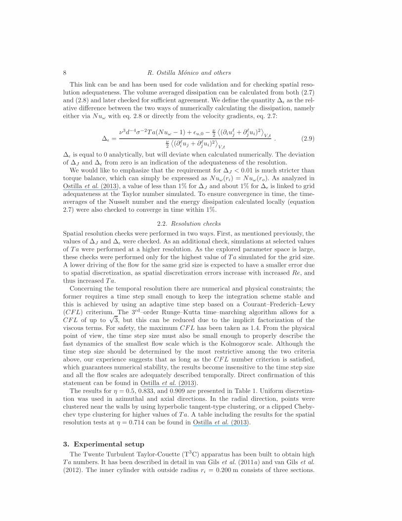
∆ǫ is equal to 0 analytically, but will deviate when calculated numerically. The deviationof ∆J and ∆ǫ from zero is an indication of the adequateness of the resolution.We would like to emphasize that the requirement for ∆J < 0.01 is much stricter than

torque balance, which can simply be expressed as Nuω(ri) = Nuω(ro). As analyzed inOstilla et al. (2013), a value of less than 1% for ∆J and about 1% for ∆ǫ is linked to gridadequateness at the Taylor number simulated. To ensure convergence in time, the time-averages of the Nusselt number and the energy dissipation calculated locally (equation2.7) were also checked to converge in time within 1%.

2.2. Resolution checks

Spatial resolution checks were performed in two ways. First, as mentioned previously, thevalues of ∆J and ∆ǫ were checked. As an additional check, simulations at selected valuesof Ta were performed at a higher resolution. As the explored parameter space is large,these checks were performed only for the highest value of Ta simulated for the grid size.A lower driving of the flow for the same grid size is expected to have a smaller error dueto spatial discretization, as spatial discretization errors increase with increased Re, andthus increased Ta.Concerning the temporal resolution there are numerical and physical constraints; the

former requires a time step small enough to keep the integration scheme stable andthis is achieved by using an adaptive time step based on a Courant–Frederich–Lewy(CFL) criterium. The 3rd–order Runge–Kutta time–marching algorithm allows for aCFL of up to

√3, but this can be reduced due to the implicit factorization of the

viscous terms. For safety, the maximum CFL has been taken as 1.4. From the physicalpoint of view, the time step size must also be small enough to properly describe thefast dynamics of the smallest flow scale which is the Kolmogorov scale. Although thetime step size should be determined by the most restrictive among the two criteriaabove, our experience suggests that as long as the CFL number criterion is satisfied,which guarantees numerical stability, the results become insensitive to the time step sizeand all the flow scales are adequately described temporally. Direct confirmation of thisstatement can be found in Ostilla et al. (2013).The results for η = 0.5, 0.833, and 0.909 are presented in Table 1. Uniform discretiza-

tion was used in azimuthal and axial directions. In the radial direction, points wereclustered near the walls by using hyperbolic tangent-type clustering, or a clipped Cheby-chev type clustering for higher values of Ta. A table including the results for the spatialresolution tests at η = 0.714 can be found in Ostilla et al. (2013).

3. Experimental setup

The Twente Turbulent Taylor-Couette (T3C) apparatus has been built to obtain highTa numbers. It has been described in detail in van Gils et al. (2011a) and van Gils et al.(2012). The inner cylinder with outside radius ri = 0.200 m consists of three sections.

Optimal Taylor-Couette flow: Radius ratio dependence 9

η Ta Nθ x Nr x Nz Nuω 100∆J 100∆ǫ Case0.5 2.5 · 105 100x100x100 2.03372 0.30 1.11 R0.5 2.5 · 105 150x150x150 2.03648 0.76 0.89 E0.5 7.5 · 105 150x150x150 2.56183 0.47 0.92 R0.5 7.5 · 105 256x256x256 2.55673 0.74 0.31 E0.5 1 · 107 300x300x300 4.23128 0.33 1.07 R0.5 1 · 107 400x400x400 4.22574 0.97 1.06 E0.5 2.5 · 107 350x350x350 5.07899 0.85 1.12 R0.5 2.5 · 107 512x512x512 5.08193 0.87 1.98 E0.5 5 · 107 768x512x1536 6.08284 0.45 1.56 R0.5 1 · 108 768x512x1536 7.48561 1.46 0.88 R

0.833 2.5 · 105 180x120x120 2.72293 0.21 0.76 R0.833 2.5 · 105 300x180x180 2.72452 0.29 0.29 E0.833 1 · 107 384x264x264 7.07487 0.29 0.61 R0.833 1 · 107 512x384x384 7.17245 0.13 1.16 E0.833 2.5 · 107 512x384x384 8.62497 0.71 1.05 R0.833 2.5 · 107 768x576x576 8.51678 0.90 1.26 E0.833 5 · 107 512x384x384 9.68437 0.26 2.92 R0.833 1 · 108 768x576x576 11.4536 0.89 2.29 R0.909 2.5 · 105 180x120x120 2.31902 0.16 0.91 R0.909 2.5 · 105 300x200x200 2.30810 0.07 0.17 E0.909 2 · 106 256x180x180 3.76826 0.55 0.49 R0.909 2 · 106 384x256x256 3.77532 0.39 0.21 E0.909 2.5 · 107 384x256x256 7.83190 0.43 3.15 R0.909 2.5 · 107 450x320x320 7.86819 0.81 2.07 E0.909 5 · 107 2305x400x1536 9.74268 0.46 1.02 R0.909 1 · 108 2305x400x1536 11.3373 0.57 1.06 R

Table 1: Resolution tests for Γ = 2π and η = 0.5, 0.833 and 0.909. The first columndisplays the radius ratio, the second column displays the Taylor number, the third columndisplays the resolution employed, the fourth column the calculated Nuω, the fifth columnand sixth colums the relative discrepancies ∆J and ∆ǫ, and the last column the ’case’:(R)esolved and (E)rror reference. ∆ǫ is positive, and exceeds the 1% threshold reportedin Ostilla et al. (2013) for some cases at the largest η, but even so resolution appears tobe sufficient as variations of Nuω are small.

The total height of those axially stacked sections is L = 0.927 m. We measure the torqueonly on the middle section of the inner cylinder, which has a height of Lmid = 0.536 m,to reduce the effect of the torque losses at the end-plates in our measurements. Thisapproach has already been validated in van Gils et al. (2012). The transparent outercylinder is made of acrylic and has an inside radius of ro = 0.279 m. We vary the radiusratio by reducing the diameter of the outer cylinder by adding a ‘filler’ that is fixed tothe outer cylinder and sits between the inner and the outer cylinder, effectively reducingro while keeping ri fixed. We have 3 fillers giving us 4 possible outer radii: ro = 0.279 m(without any filler), 0.26 m, 0.24 m, and 0.22 m, giving experimental access to η = 0.716,0.769, 0.833, and 0.909, respectively. Note that by reducing the outer radius, we not onlychange η, but also change Γ = L/(ro − ri) from Γ(η = 0.716) = 11.68 to Γ(η = 0.909) =46.35.

For high Ta the heating up of the system becomes apparent and it has to be activelycooled in order to keep the temperature constant. We cool the working fluid (water)

10 R. Ostilla Monico and others

from the top and bottom end plates and maintain a constant temperature within ±0.5Kthrought both the spatial extent and the time run of the experiment. The setup has beenconstructed in such a way that we can rotate both cylinders independently while keepingthe setup cooled.As said before, we measure the torque on the middle inner cylinder. We do this by

measuring the torque that is transferred from the axis to the cylinder by using a load-cellthat is inside the aforementioned cylinder. Torque measurements are performed usinga fixed procedure: the inner cylinder is spun up to its maximum rotational frequencyof 20 Hz and kept there for several minutes. Then the system is brought to rest. Thecylinders are then brought to their initial rotational velocities (with the chosen 1/Ro),corresponding to a velocity for which the torque is accurate enough; generally of order2–3 Hz. We then slowly increase both velocities over 3-6 hours to their final velocitieswhile maintaining 1/Ro fixed during the entire experiment. During this velocity rampwe continuously acquire the torque of this quasi-stationary state. The calibration of thesystem is done in a similar way; first we apply the maximum load on the system, goingback to zero load, and then gradually adding weight while recording the torque. Theseprocedures ensure that hysteresis effects are kept to a minimum, and that the system isalways brought to the same state before measuring. More details about the setup can befound in van Gils et al. (2011a).Local velocity measurements are done by laser Doppler anemometry (LDA). We mea-

sure the azimuthal velocity component by focusing two beams in the radial-azimuthalplane. We correct for curvature effects of the outer cylinder by using a ray-tracer, seeHuisman et al. (2012a). The velocities are measured at midheight (z = L/2) unless spec-ified otherwise. For every measurement position we measured long enough such as to havea statistically stationary result, for which about 105 samples were required for every datapoint. This ensured a statistical convergence of < 1%.

4. Global response: Torque

In this section, the global response of the TC system for the four simulated radius ratiosis presented. This is done by measuring the scaling law(s) of the non-dimensional torqueNuω as function(s) of Ta. The transition between different types of local scaling lawsin different Ta-ranges is investigated, and related to previous simulations (Ostilla et al.

2013) and experiments (van Gils et al. 2012).

4.1. Pure inner cylinder rotation

The global response of the system is quantified by Nuω. By definition, for purely az-imuthal laminar flow, Nuω = 1. Once the flow is driven stronger than a certain criticalTa, large azimuthal roll structures appear, which enhance angular transport through alarge scale wind.Figure 4 shows the response of the system for increasing Ta in case of pure inner

cylinder rotation for four values of η. Experimental and numerical results are shown inthe same panels, covering different ranges and thus complementary, but consistent witheach other. Numerical results for η = 0.714 from Ostilla Monico et al. (2013) have beenadded to both panels.As has already been noticed in Ostilla et al. (2013) for η = 0.714, a change in the local

scaling law relating Ta to Nuω occurs at around Ta ≈ 3 · 106. We can interpret thesechanges in the same way as Ostilla et al. (2013) and relate the transition in the Ta-Nuω

local scaling law to the break up of coherent structures.It is also worth mentioning that the exponent in the local scaling laws in the regime

Optimal Taylor-Couette flow: Radius ratio dependence 11

104

105

106

107

108

109

1010

1011

1012

1013

10−1

100

101

102

103

Nu

ω-1

Ta

η = 0.5η = 0.714η = 0.769η = 0.833η = 0.909

104

105

106

107

108

109

1010

1011

1012

1013

0.01

0.02

0.03

0.04

0.05

(Nu

ω-1)/

Ta0.3

3

Ta

0.20 ( - 0.33)

0.39 ( - 0.33)

Figure 4: The global system response for pure inner cylinder rotation as function of thedriving Ta: The top panel shows Nuω − 1 vs Ta for both simulations (points on the leftof the graph) and experiments (lines on the right of the graph). Numerical data fromOstilla Monico et al. (2013) for η = 0.714 have been added to these figures. The bottompanel shows the compensated Nusselt ((Nuω − 1)/Ta1/3) versus Ta, with added lineswith scaling law Ta0.20 and Ta0.39 to guide the eye.

before the transition depends on the radius ratio. This can be seen in the compensatedplot, and explains the curve crossings that we see in the graphs.For experiments (solid lines of figure 4), a different local scaling law can be seen.

In this case the experiments are performed at much higher Ta than the simulations.The scaling Nuω ∼ Ta0.38 can be related to the so called “ultimate” regime, a regimewhere the boundary layers have become completely turbulent (Grossmann & Lohse 2011,2012; Huisman et al. 2013). As indicated for the case at η = 0.714 we expect that forincreasing Ta also the simulations become turbulent enough to reach this scaling law (cf.Ostilla Monico et al. (2013)). In this regime, the local scaling law relating Ta and Nuω

has no dependence on η and thus is universal.In both experiment and simulation with the largest Ta, the value of η corresponding

to the smallest gap, i.e. η = 0.909, has the highest angular velocity transport (Nuω)at a given Ta. This can be phrased in terms of the pseudo-Prandtl-number σ, intro-duced in EGL2007. As a smaller gap means a smaller σ, we thus find a decrease ofNuω with increasing σ, for the drivings explored in experiments, similarly as predicted

12 R. Ostilla Monico and others

Grossmann & Lohse (2001) and found Xia et al. (2002) for Nu(Pr) in RB convection forPr > 1.

4.2. Rossby number dependence

In this subsection, the effect of outer cylinder rotation on angular velocity transport willbe studied. Previous experimental and numerical work at η = 0.714 (Paoletti & Lathrop2011; van Gils et al. 2011b; Ostilla et al. 2013; Brauckmann & Eckhardt 2013a) revealedthe existence of an optimum transport where, for a given Ta, the transport of momentumis highest at a Rossby number Ro−1

opt, which depends on Ta and saturates around Ta ∼1010. In this subsection, this work will be extended to the other values of η.Figure 5 shows the results of the numerical exploration of the Ro−1 parameter space

between Ta = 4 · 104 and Ta = 2.5 · 107. The shape of Nuω = Nuω(Ro−1) curves and theposition of Ro−1

opt depends very strongly on η in the Ta range studied in numerics. For thelargest gap (i.e., η = 0.5), the optimum can be seen to be in the counter–rotating range(i.e., Ro−1 < 0) as long as Ta is high enough. On the other hand, for the smallest gap (i.e.,η = 0.909), the optimum is at co–rotation (i.e., Ro−1 > 0) in the whole region studied.The other values of studied η reveal an intermediate behavior. Optimum transport islocated for co–rotation at lower values of Ta and slowly moves towards counter–rotation.For all values of η, when the driving is increased, Ro−1

opt tends to shift to more negativevalues.For two values of Ta (Ta = 4 · 106 and Ta = 107) for a radius ratio η = 0.5, two

distinct peaks can be seen in the Nuω(Ro−1) curve. This can be understood by lookingat the flow topology. For Ro−1 = 0, three distinct rolls can be seen. However, whendecreasing Ro−1, the rolls begin to break up. Some remnants of large-scale structurescan be seen, but these are weaker than the Ro−1 = 0 case. Having a large-scale roll helpsthe transport of angular momentum, leading to the peak in Nuω at Ro−1 = 0. Furtherincreasing the driving causes the rolls to also break up for Ro−1 = 0, and eliminates theanomalous peak.The shift seen in the numerics may or may not continue with increasing Ta. The

experiments conducted explore a parameter space of 1010 < Ta < 1013 and thus serveto explore the shift at higher driving. Figure 6 presents the obtained results. The leftpanel shows Nuω versus Ta for all measurements. The right panel shows the exponentγ, obtained by fitting a least-square linear fit in the log–log plots. Across the η andRo−1 range studied, the average exponent is γ ≈ 0.39. This value is used in figure 7 tocompensate Nuω. The horizontality of all data points reflects the good scaling and theuniversality of this ultimate scaling behaviour Nuω ∝ Ta0.39.To determine the optimal rotation ratio for the experimental data, a Ta-averaged

compensated Nusselt 〈Nuω/Ta0.39〉Ta was used. This is defined as:

〈Nuω/Ta0.39〉Ta =

1

Tamax − Taco

∫ Tamax

Taco

Nuω/Ta0.39dTa, (4.1)

where Tamax is the maximum value of Ta for every (η,Ro−1) dataset, and Taco is acut-off Ta number used for the larger η (Taco = 2 · 1011 for η = 0.833 and Taco = 3 · 1010for η = 0.909) to exclude the initial part of the Nuω/Ta

0.39 data points which seem tohave a different scaling for some of the values of Ro−1 explored. For the smaller valuesof η, Taco = Tamin, the minimum value of Ta for every (η,Ro−1) dataset. An error baron this average is estimated as one standard deviation of the data from the computedaverage.The two panels of figure 8 show 〈Nuω/Ta

0.39〉Ta as a function of Ro−1 or alternatively

Optimal Taylor-Couette flow: Radius ratio dependence 13

−1.5 −1 −0.5 0 0.50

1

2

3

4

5N

uω-1

1/Ro

Ta=4e4

Ta=1.0e5

Ta=2.5e5

Ta=7.5e5

Ta=2.0e6

Ta=4.0e6

Ta=1.0e7

Ta=2.5e7

η = 0.5

−0.8 −0.6 −0.4 −0.2 0 0.2 0.4 0.6 0.80

2

4

6

8

Nu

ω-1

1/Ro

Ta=3.90e4Ta=1.03e5Ta=2.44e5Ta=7.04e5Ta=1.91e6Ta=3.90e6Ta=9.52e6Ta=2.39e7

η = 0.714

−0.5 0 0.5 10

2

4

6

8

Nu

ω-1

1/Ro

Ta=4e4

Ta=1.0e5

Ta=2.5e5

Ta=7.5e5

Ta=2.0e6

Ta=4.0e6

Ta=1.0e7

Ta=2.5e7

η = 0.833

−0.2 0 0.2 0.4 0.6 0.8 10

2

4

6

8

Nu

ω-1

1/Ro

Ta=4e4

Ta=1.0e5

Ta=2.5e5

Ta=7.5e5

Ta=2.0e6

Ta=4.0e6

Ta=1.0e7

Ta=2.5e7

η = 0.909

Figure 5: Nuω − 1 versus Ro−1 for the four values of η studied numerically, η = 0.5(top), 0.714, 0.833 and 0.909 (bottom). The shape of the curve and the position of themaximum depend very strongly on both Ta and η.

14 R. Ostilla Monico and others

1010

1011

1012

101310

1

102

103

Ta

Nu

ω

η = 0.716η = 0.769η = 0.833η = 0.909

−0.5 −0.25 0 0.25

0.36

0.38

0.4

0.42

0.44

1/Ro

γ

η = 0.716; γ = 0.39 ± 0.03η = 0.769; γ = 0.41 ± 0.01η = 0.833; γ = 0.39 ± 0.02η = 0.909; γ = 0.39 ± 0.03

Figure 6: The left panel shows Nuω versus Ta for all values of η and Ro−1 studied inexperiments. The right panel shows the exponent γ of the scaling law Nuω ∝ Taγ forvarious Ro−1, obtained by a least-square linear fit in log-log space. The average value ofγ for each η is represented by the dashed lines, while the solid line represents the averagevalue of γ = 0.39 for all η, which will be used for compensating Nuω.

of a for the four values of η considered in experiments. The increased driving changesthe characteristics of the flow. This is reflected in the very different shapes of the Ro−1-dependence of Nuω when comparing figures 5 and 8, and in the shift of Ro−1

opt.To summarize these effects, figure 9 presents both the 95% peak width ∆Ro−1

max andthe position of optimal transport Ro−1

opt determined as the realization with the maximumtorque as a function of Ta and η obtained from numerics as well as the asymptotic valuefrom experiments. The peak width ∆Ro−1

max is defined as:

∆Ro−1

max =

∫ Ro−1

0.95

Ro−1

−0.95

Nuω(Ro−1)dRo−1

max(Nuω − 1)(4.2)

where Ro−1

−0.95 and Ro−1

0.95 are the values of Ro−1 for which Nuω is 95% of the peak value.The 95% peak width can be seen to vary with driving, reflecting what is seen in figure

5. The shape of the Ro−1-Nuω curve is highly dependent of both η and Ta. Ro−1

opt shows

a very large variation across the Ta range studied in numerics. The shift of the Ro−1

opt

with Ta is expected to continue until it reaches the value found in the experiments. Thiscan be seen in the right panel of figure 5 for η = 0.5 to η = 0.833. For η = 0.909 , thetrend seems to change for the last point. However, this is due to the very large and flatpeak of the Nuω(Ro−1) curve- this can also be seen in the left panel and in figure 5d.One may also ask the question: has the value of Ro−1

opt already saturated in our experi-ments? Figure 7 shows the trend for Nuω for increasing Ta. This trend does not seem tovary much for different values of Ro−1. Therefore, we expect the value of Ro−1

opt to havealready reached saturation in our experiments.We can compare these new experimental results to the available results from the

literature, the speculation made in van Gils et al. (2012) and the prediction made inBrauckmann & Eckhardt (2013b) for the dependence of the saturated aopt on η. This isshown in figure 10. Both dependencies are shown to deviate substantially from the exper-imental results obtained in the present work. Even if the speculation from van Gils et al.(2012) appears to be better for this η-range, for previous experimental data at η = 0.5,it is in clear difference with the experimentally measured value for optimal transport byMerbold et al. (2013).

Optim

alTaylor-C

ouette

flow:Radiusratio

depen

den

ce15

1011

1012

1013

0

0.002

0.004

0.006

0.008

0.01

0.012

Ta

Nu

ω/T

a0.39

η = 0.716

= -0.53

-0.40

-0.33

-0.31

-0.30

-0.28

-0.26

-0.25

-0.23

-0.21

-0.21

-0.18

-0.16

-0.13

-0.10

-0.07

0.00

0.13

0.20

0.53

1/Ro

1011

1012

1013

0

0.002

0.004

0.006

0.008

0.01

0.012

Ta

Nu

ω/T

a0.39

η = 0.769

1/Ro = -0.40

-0.36

-0.30

-0.27

-0.23

-0.21

-0.20

-0.19

-0.17

-0.16

-0.16

-0.14

-0.12

-0.10

-0.00

0.11

0.26

1011

1012

0

0.002

0.004

0.006

0.008

0.01

0.012

Ta

Nu

ω/T

a0.39

η = 0.833

1/Ro = -0.267

-0.241

-0.201

-0.178

-0.150

-0.142

-0.134

-0.124

-0.121

-0.117

-0.115

-0.110

-0.104

-0.100

-0.093

-0.080

-0.067

0.0

0.071

0.172

1010

1011

0

0.002

0.004

0.006

0.008

0.01

0.012

Ta

Nu

ω/T

a0.39

η = 0.909

1/Ro = -0.133

-0.120

-0.100

-0.089

-0.075

-0.067

-0.062

-0.060

-0.057

-0.052

-0.046

-0.033

0.00

0.035

0.060

0.086

0.107

Figure

7:Thefourpanels

show

Nuω/Ta0.39vs.

Taforallexplored

values

ofRo−1for

thefourstu

died

values

ofη:η=

0.714(to

p-left),

0.769(to

p-rig

ht),

0.833(botto

m-left),

and0.909(botto

m-rig

ht).

Thesca

linglaw

Nuω∼

Ta0.39is

seento

approx

imately

hold

throughoutthewhole

parameter

space

explored

.Notren

dscanbeapprecia

tedwhich

would

leadusto

expect

furth

ershift

oftheoptim

um

with

increa

seddriv

ing.Dashed

lines,

indica

tingthecut-o

ffreg

ionsused

fordeterm

ining〈N

uω/Ta0.39〉

Tahavebeen

plotted

for

η=

0.833andη=

0.909.

16 R. Ostilla Monico and others

−0.4 −0.2 0 0.2 0.4 0.62

4

6

8

10

x 10−3

〈Nu

ω/Ta0.3

9〉 T

a

1/Ro

η = 0.714η = 0.769η = 0.833η = 0.909

−0.2 −0.1 0

8

8.5

9

9.5

x 10−3

1/Ro

−0.5 0 0.5 1 1.5 22

4

6

8

10

x 10−3

〈Nu

ω/Ta0.3

9〉 T

a

a

0.2 0.4 0.6

8.5

9

9.5

x 10−3

a

η = 0.714

η = 0.769

η = 0.833

η = 0.909

Figure 8: The panels show 〈Nuω/Ta0.39〉Ta versus either Ro−1 (top) or a (bottom) at

the cut-off region highlighted in figure 7 for the values of η studied experimentally. Insetscontaining a zoom-in around the optimum have been added for clarity. Error bars indicateone standard deviation from the mean value, and are too small to be seen for most datapoints. There is a strong η-dependence of the curve Nuω/Ta

0.39 versus Ro−1, even at thelargest drivings studied in experiments. Optimal transport is located atRo−1

opt = −0.20 for

η = 0.714, Ro−1

opt = −0.15 for η = 0.769, Ro−1

opt = −0.10 for η = 0.833 and Ro−1

opt = −0.05for η = 0.909, corresponding to a ≈ 0.33− 0.35 for all values of η. In the bottom panel,the maximum of the graph is less pronounced, i.e. it becomes more flat with increasingη. In the limit η → 1, a does not tend to a finite limit, while Ro−1 does. This resulthighlights the advantage of using Ro−1 instead of a as a control parameter.

This section has shown that the radius ratio has a very strong effect on the globalresponse and especially on optimal transport. Significantly increased transport for co–rotation has been found at the lowest drivings based on the DNS results. This findingwas already reported in Ostilla et al. (2013) for η = 0.714, but the transport increasewas marginal. For η = 0.833 and especially for η = 0.909 the transport can be increasedup to three times. The shift of Ro−1

opt has also been seen to be much bigger and to happenin a much slower way for smaller gaps. The reason for this will be studied in Section 5,using the local data obtained from experiments and numerics.

Optimal Taylor-Couette flow: Radius ratio dependence 17

104

106

108

0

0.05

0.1

0.15

0.2

∆R

o−1

max

Ta10

410

610

8−0.4

−0.2

0

0.2

0.4

1/R

o opt

Ta

η = 0.5

η = 0.714

η = 0.833

η = 0.909

Figure 9: In the left panel, 95% peak width ∆Ro−1max vs Ta for the four values of η

analyzed in numerics. The peak width can be seen to vary with driving, and for smallergaps is larger for larger values of Ta. In the right panel, Ro−1

opt vs Ta for the same fourvalues of η. The location of the optimal transport has a very strong dependence on thedriving, especially for the largest values of η. As driving increases beyond the numericallystudied range and overlaps with experiments, Ro−1

opt should tend to the experimentallyfound values, represented as dashed lines in the figure. The asymptote for η = 0.5 isobtained from Merbold et al. (2013). The trend appears to be less clear for η = 0.909,but this might be understandable from the peak width at the highest driving Ta.

0.4 0.6 0.8 1

0.2

0.3

0.4

0.5

η

aopt

van Gils et. alBrauckmann & EckardtMerbold et. al (2013)WendtBrauckmann & Eckhardt DNSPaoletti & LathropPresent work

Figure 10: State-of-the-art data for aopt(η), from both experiments (Wendt 1933;Paoletti & Lathrop 2011; Merbold et al. 2013) and numerics (Brauckmann & Eckhardt2013b). The speculation of van Gils et al. (2012) and the prediction ofBrauckmann & Eckhardt (2013b) are plotted as lines on the graph. The new ex-perimental results deviate up substantially from both predictions, even when taking intoaccount error bars.

5. Local results

In this section, the local angular velocity profiles will be analyzed. Angular velocity isthe transported quantity in TC flow and shows the interplay between the bulk, wherethe transport is convection dominated, and the boundary-layers, where the transport isdiffusion dominated. Numerical profiles and experimental profiles obtained from LDAwill be shown. The angular velocity gradient in the bulk will be analyzed and connectedto the optimal transport. In addition, the boundary layers will be analyzed and compared

18 R. Ostilla Monico and others

0 0.5 10

0.2

0.4

0.6

0.8

1

〈ω〉 z

r

1/Ro=0.500.220.00−0.18−0.33−0.57−0.75−1.00−1.20

η = 0.5

0 0.5 10

0.2

0.4

0.6

0.8

1

〈ω〉 z

r

1/Ro=0.530.200.00−0.07−0.14−0.23−0.30−0.40−0.48

η = 0.714

0 0.5 10

0.2

0.4

0.6

0.8

1

〈ω〉 z

r

1/Ro=0.600.400.270.100.040.0−0.07−0.11−0.20−0.27

η = 0.833

0 0.5 10

0.2

0.4

0.6

0.8

1〈ω

〉 z

r

1/Ro=0.470.200.130.050.020.00−0.02−0.05−0.08−0.12

η = 0.909

Figure 11: Azimuthally, axially and temporally averaged angular velocity 〈ω〉z versusradius r for: η = 0.5, η = 0.714, η = 0.833, and η = 0.909. Data is for Ta = 2.5 · 107(Ta = 2.39 ·107 for η = 0.714) and selected values of Ro−1. For smaller η, the ω-bulkprofiles differ more from a straight line, and have, on average, a smaller value.

to the results from the analytical formula from EGL 2007 for the BL thickness ratio inthe non-ultimate regime.

5.1. Angular velocity profiles

Angular velocity ω profiles obtained from numerics are shown in figure 11. Results arepresented for four values of η and selected values of Ro−1 at Ta = 2.5 · 107 (and Ta =2.39 · 107 for η = 0.714). Experimental data obtained by using LDA are shown in figure12 for three values of η: from top-left to bottom, η = 0.714 for Rei−Reo = 106, η = 0.833for Ta = 5 · 1011, and η = 0.909 for Ta = 1.1 · 1011.The different radius ratios affect the angular velocity profiles on both boundary layers,

as the two boundary layers are more asymmetric for the wide gaps; and they affect thebulk, as the bulk angular velocity is smaller for wide gaps. These effects will be analyzedin the next sections.

5.2. Angular velocity profiles in the bulk

We now analyze the properties of the angular velocity profiles in the bulk. We find thatthe slope of the profiles in the bulk is controlled mainly by Ro−1 and less so by Ta. Thiscan be understood as follows: The Taylor number Ta acts through the viscous term,dominant in the boundary layers, while Ro−1 acts through the Coriolis force, present inthe whole domain. These results extend the finding from Ostilla et al. (2013) to othervalues of η.

Optimal Taylor-Couette flow: Radius ratio dependence 19

0.2 0.4 0.6 0.80.2

0.3

0.4

0.5

0.6

〈ω〉 z

r

1/Ro=0.340.200.090.00−0.07−0.13−0.18−0.20−0.23−0.27−0.30−0.33−0.40−0.53

η = 0.714

0.2 0.4 0.6 0.80.2

0.3

0.4

0.5

0.6

〈ω〉 z

r

1/Ro=0.00−0.07−0.09−0.11−0.13−0.15−0.18−0.20−0.24−0.27

η = 0.833

0.2 0.4 0.6 0.80.2

0.3

0.4

0.5

0.6

〈ω〉 z

r

1/Ro=0.00−0.03−0.05−0.06−0.07−0.08−0.09−0.10−0.13

η = 0.909

Figure 12: Angular velocity profiles obtained by LDA for η = 0.714 at either Rei−Reo =106 (top), η = 0.833 or at Ta = 5 · 1011 (bottom-left) and η = 0.909 at Ta = 1.1 · 1011(bottom-right), to explore different dependencies in parameter space. Data is taken at afixed axial height (ie. the cylinder mid-height, z = L/2), but as the Taylor number Ta ismuch larger than in the numerics, the axial dependence is much weaker.

To further quantify the effect of Ro−1 on the bulk profiles, we calculate the gradient of〈ω〉z . For the DNS data, this is done by numerically fitting a tangent line to the profileat the inflection point using the two neighboring points on both sides (at a distance of0.01− 0.02 r-units); such fit is shown in the left panel of figure 13.As the spatial resolution of the LDA data is more limited, the fit is done differently.

A linear regression to the ω-profile between 0.2 < r < 0.8 is done. The larger range ofr is chosen in experiments because: (i) the boundary layers are small enough due to thehigh Ta that they are outside of the fitting range, and (ii) the fluctuations of the dataare much higher in experiments, especially for the LDA of the narrow gaps (η = 0.833and η = 0.909). From this regression, we calculate 〈ω〉z, and an error taken from thecovariance matrix of the fit.Figure 14 shows four panels, each containing the angular velocity gradient in the bulk

from the numerical simulations and experiments for a given value of η. We first notice thatthe angular velocity gradients from experiment and numerics are in excellent agreement.Next the connection between a flat angular velocity profile and optimal transport for thehighest drivings explored in the experiments can now be seen for other values of η and notjust for η = 0.714 as reported previously (van Gils et al. 2011b). Once Ro−1 < Ro−1

opt,the large scale balance analyzed in Ostilla et al. (2013) breaks down, and a “neutral”surface which reduces the transport appears in the flow.In simulations, because of resolution requirements, we are unable of driving the flow

strongly enough to see a totally flat bulk profile. Also, the influence of the large scale

20 R. Ostilla Monico and others

0 0.2 0.4 0.6 0.8 10

0.2

0.4

0.6

0.8

1

r

〈ω〉 z

0 0.2 0.4 0.6 0.8 10

0.2

0.4

0.6

0.8

1

r

〈uθ〉

Figure 13: An example of the two fitting procedures for the bulk angular velocity gradientand for boundary layer thicknesses done on the DNS data is shown here. Both panels showthe θ,z, and t averaged azimuthal velocity and angular velocity for η = 0.5, Ta=1 ·107,and pure inner cylinder rotation. In the left panel a line is fitted to the bulk of the angularvelocity to obtain the bulk gradient. The dashed lines indicate the EGL approximation.The right panel shows the three-lines-fit to the whole profile to obtain the width of itsboundary layers, used in Section 5.3. Both bulk fits are done at the inflection point, butfor different variables (ω or uθ), which gives slightly different slopes (and intersectionpoints).

structures causes a small discrepancy between the flattest profile and the value of Ro−1

opt

measured from Nuω. This is expected to slowly dissapear with increasing Ta.In Ostilla et al. (2013), a linear extrapolation of the bulk angular velocity gradient

was done to give an estimate for the case when this profile would become horizontal, i.e.,d〈ω〉z/dr = 0, and thus give an estimate of Ro−1

opt. For η = 0.714 this estimate agreedwith the numerical result within error bars. Here, we extend this analysis for the othervalues of η and, as we shall see, successfully.As in Ostilla et al. (2013), an almost linear relationship between Ro−1 and d〈ω〉z/dr

can be seen. This linear relationship is extrapolated and plotted in each panel. Thisextrapolation gives an estimate for Ro−1

opt(Ta → ∞), which we can compare to the ex-

perimentally determined Ro−1

opt(Ta → ∞). For η = 0.833, Ro−1(Ta → ∞) ≈ −0.12corresponding to a ≈ 0.38 is obtained, and for η = 0.909, Ro−1(Ta → ∞) ≈ −0.05,corresponding to a ≈ 0.31 is obtained. These values are (within error bars) also obtainedfor Ro−1

opt at the large Ta investigated in experiments, namely Ro−1

opt = −0.10 and −0.05,respectively.For η = 0.5, Ro−1

opt(Ta → ∞) ≈ −0.33 is obtained, corresponding to a ≈ 0.2. This valueis consistent with the numerical results in Brauckmann & Eckhardt (2013b), which reportaopt ≈ 0.2. However, care must be taken, as fitting straight lines to the ω-profiles giveshigher residuals for η = 0.5 as the profiles deviate from straight lines (cf. top-left panelof figure 11). A fit to the “quarter-Couette” profile derived from upper bound theory(Busse 1967) is much more appropriate for η = 0.5 at the strongest drivings achieved inexperiments (Merbold et al. 2013). This is because the flow feels much more the effectof the curvature at the small η. On the other end of the scale, the linear relationshipworks best for smallest gaps, i.e. η = 0.909 (cf. the bottom right panel of figure 11) wherecurvature plays a small effect.To further elaborate the link between η, flat ω-profiles and Ro−1, data for the smallest

Optimal Taylor-Couette flow: Radius ratio dependence 21

−1 −0.5 0 0.5 1−0.5

−0.4

−0.3

−0.2

−0.1

0d〈ω

〉 z/dr

1/Ro

Ta=2e6Ta=4e6Ta=1e7Ta=2.5e7

η = 0.5

−0.5 0 0.5 1−0.8

−0.6

−0.4

−0.2

0

1/Ro

d〈ω

〉 z/dr

Ta=1.91e6Ta=3.90e6Ta=9.52e6Ta=2.39e7Re

i−Re

o=1e6 (E)

η = 0.714

−0.2 0 0.2 0.4 0.6−0.8

−0.6

−0.4

−0.2

0

d〈ω

〉 z/dr

1/Ro

Ta=2e6Ta=4e6Ta=1e7Ta=2.5e7Ta=5e11(E)

−0.15 −0.1 −0.05

−0.1

−0.05

0

η = 0.833

−0.2 0 0.2 0.4 0.6 0.8−1

−0.8

−0.6

−0.4

−0.2

0

d〈ω

〉 z/dr

1/Ro

−0.1 −0.05 0−0.2

−0.1

0

Ta=2e6Ta=4e6Ta=1e7Ta=2.5e7Ta=1.1e11(E)

η = 0.909

Figure 14: Bulk angular velocity gradient d〈ω〉z/dr against Ro−1 for the four values ofη explored in simulations, η = 0.5 (top left), η = 0.714, (top right), η = 0.833, (middle),and η = 0.909 (bottom). Data from experiments obtained by LDA is also plotted forthe three values of η for which it was experimentally measured (green circles). For allvalues of η except η = 0.5, for co–rotation and slight counter–rotation there is onceagain an almost linear relationship between Ro−1 and d〈ω〉z/dr. A black straight line isadded to extrapolate this relationship in order to estimate Ro−1

opt. A plateau, in whichthe radial gradient of 〈ω〉z is small can be seen around optimal transport, indicating alarge convective transport of angular velocity.

gap η = 0.95 from Wendt (1933) has been digitized, and d〈ω〉z/dr was been determinedfor it. This data corresponds to a driving of Ta ∼ 108 − 109. Figure 15 shows d〈ω〉z/dragainst Ro−1 for Wendt’s data and also for the current experimental data. The flattestprofile can be seen to occur for increasing (in absolute value) Ro−1 for larger gaps,simular to the shift of Ro−1. For η = 0.95, almost no curvature is felt by the flow and aflat profiles can be seen for −0.05 < Ro−1 < 0. However, adding a Coriolis force (in the

22 R. Ostilla Monico and others

−0.5 0 0.5 1−0.8

−0.6

−0.4

−0.2

0

〈dω/dr〉

z

1/Ro

−0.2 −0.1 0−0.2

−0.1

0

η = 0.714

η = 0.833

η = 0.909

η = 0.95 (Wendt)

Figure 15: Bulk angular velocity gradient d〈ω〉z/dr against Ro−1 for the three values of ηexplored in experiments, and for η = 0.95 (digitized from Wendt (1933)). The error barsof Wendt’s data are larger due to the quality of the digitization. As seen previously, theflattest profile occurs around weak counter-rotation, for all values of η including η = 0.95.

form of Ro−1) a large ω-gradient is sustained in the bulk. This corroborates the balancebetween Ro−1 and the bulk ω-gradients proposed in Ostilla et al. (2013).

5.3. Angular velocity profiles in the boundary layers in the classical turbulent regime

As the driving is increased, the transport is enhanced. To accommodate for this, theboundary layers (BLs) become thinner and therefore the ω-slopes (∂rω) become steeper.Due to the geometry of the TC system an intrinsic asymmetry in the BL layer widths ispresent. More precisely, the exact relationship ∂r〈ω〉|o = η3∂r〈ω〉|i holds for the slopesof the boundary layers, due to the r independence of Jω, cf. EGL 2007 and eq.(2.4).An analysis of the boundary layers was not possible in the present experiments because

the present LDA measurements have insufficient spatial resolution to resolve the flow inthe near–wall region. Therefore, only DNS results will be analyzed here. In simulationsthe driving is not as large as in experiments, and as a consequence the shear in the BLsis expected to not be large enough to cause a shear-instability. This means that the BLsare expected to be of Prandtl-Blasius (i.e. laminar) type, even if the bulk is turbulent.On the other hand, in the experiments both boundary layers and bulk are turbulent, i.e.the system is in the “ultimate regime”.Using the DNS data, we can compare the ratio of the numerically obtained boundary

layer widths with the analytical formula for this ratio obtained by EGL 2007 for laminarboundary layers, namely:

λoω

λiω

= η−3|ωo − ωbulk||ωi − ωbulk|

, (5.1)

where the value of ωbulk is some appropriate value in between for which the angularvelocity at the inflection point of the profile might be chosen, i.e., the point at which thelinear bulk profile fit was done to obtain λo

ω and λiω. The value ωbulk is taken from the

numerics, and may bias the estimate.To calculate the boundary layer thicknesses, the profile of the mean azimuthal velocity

〈uθ〉z is approximated by three straight lines, one for each boundary layer and one for thebulk. For the boundary layers the slope of the fit is calculated by fitting (by least-mean-squares) a line through the first two computational grid points. For the bulk, first theline is forced to pass through the grid point which is numerically closest to the inflectionpoint of the profile. Then its slope is taken from a least mean square fit using two grid

Optimal Taylor-Couette flow: Radius ratio dependence 23

points on both sides of this inflection point. The respective boundary layer line will crosswith this bulk line at a point which then defines the thickness of that boundary layer.The results obtained for λo

ω/λiω both from equation 5.1 and directly from the simula-

tions is shown in figure 14. Results are presented for the four values of η and only forthe highest value of Ta achieved in the simulations. The boundary layer asymmetry forcounter–rotating cylinders (i.e., Ro−1 < 0) grows with larger gaps. This is to be expected,as the η−3 term is much larger (≈ 8) for the largest gap as compared to the smallest gap(≈ 1.3). This is consistent with the η and thus σ restriction in EGL 2007 to a range ofsmaller gap widths.As noticed already in Ostilla et al. (2013) we find that the fit is not satisfactory for

co–rotation (i.e., Ro−1 > 0) at the lowest values of η, but is satisfactory for counter–rotation (ie. Ro−1 < 0). In EGL 2007, equation (5.1) is obtained by approximatingthe profile by three straight lines, two for the BLs and a constant ω line for the bulk.Therefore, we expect the approximation to hold best when the bulk has a flat gradient.For co–rotating cylinders and strongly counter–rotating cylinders, the bulk has a steepgradient (see figure 14), but characteristically different shapes. The only free parameterin equation (5.1) is ωbulk, which is chosen to be ω at the point of inflection. Due tothe different shapes of the ω-profiles, this choice seems more correct for counter-rotatingcylinders, as there is a clear inflection point in the profile. On the other hand, for co-rotating cylinders, the profile appears to be more convex-like, and there, the choice ofωbulk as the inflection point induces errors in the approximation (cf. 13a). For η = 0.5,the error from the constant ω approximation is even more pronounced, and the formulafails.For co–rotation the boundary layers are approximately of the same size, and the ratio

λoω/λ

iω is very close to 1. If one inverts equation (5.1) by aproximating this ratio by 1,

an estimate of what the angular velocity will be in the bulk due to the boundary layerslope asymmetry is obtained:

ωbulk =η3

1 + η3, (5.2)

corresponding to:

ωℓbulk =

−ωℓo + η3ωℓ

i

1 + η3, (5.3)

in the lab frame. This expression gives an estimate for ωbulk when the profile is flattest,and has been represented graphically in figure 11. Indeed, one can take this estimate (forexample 0.27 for η = 0.714) and compare it with figures 11 and 12. We note that thevalue of ω in the bulk for the flattest profile in the numerics (at Ro−1 ≈ Ro−1

opt(Ta)) lies

around ωbulk. We can also notice that the profiles for Ro−1 > Ro−1

opt approximately crosseach other at the same point, and this point has a value of ω ≈ ωbulk. This effect can onlybe seen in the numerics, as these approximations break down once the boundary layersbecome turbulent. The cross points of the curves are taken as an estimate for ωbulk, andthis is represented against eq. 5.2 in figure 17.To understand why the boundary layers are of approximately the same thickness de-

spite the different initial slopes at the cylinders one has to go back to equation (2.4). Theangular velocity current has a diffusive part and a convective part. Per definition in theboundary layer the diffusion dominates and in the bulk the convection does. Thus theboundary layer ceases when convection becomes significant. But convection is controlledby the wind. Thus in essence the boundary layer size is controlled by the wind and not

24 R. Ostilla Monico and others

−1 −0.5 0 0.50

2

4

6

8

1/Ro

λo ω/λ

i ω

η = 0.5

−0.2 −0.1 0 0.1 0.20

1

2

3

4

5

6

1/Ro

λo ω/λ

i ω

EGLNumerics

η = 0.714

−0.2 0 0.2 0.4 0.60

1

2

3

1/Ro

λo ω/λ

i ω

η = 0.833

−0.1 0 0.1 0.2 0.3 0.40

0.5

1

1.5

2

1/Ro

λo ω/λ

i ωη = 0.909

Figure 16: λoω/λ

iω from simulations (dots) and from equation (5.1) (solid lines) versus

Ro−1 for the four values of η studied numerically, η = 0.5 (top-left), 0.714 (top-right),0.833 (bottom-left) and 0.909 (bottom-right) at Ta = 2.5 · 107. The numerical results andthe estimate from equation (5.1) match very well for larger values of η and especially forcounter–rotating cylinders (1/Ro < 0). The asymmetry between the boundary layers canbe seen to be larger for smaller values of η, which is expected as equation (5.1) containsthe explicit factor η−3.

0 0.2 0.4 0.6 0.8 10

0.1

0.2

0.3

0.4

0.5

η

ωbulk

Equation (5.2)DNS data

Figure 17: ωbulk as a function of η, taken from both eq. 5.2 and from the crosspoints ofthe ω-profiles in figure 11. The trend is the same in both data sets. A smaller value of ηdecreases the value of the bulk angular velocity.

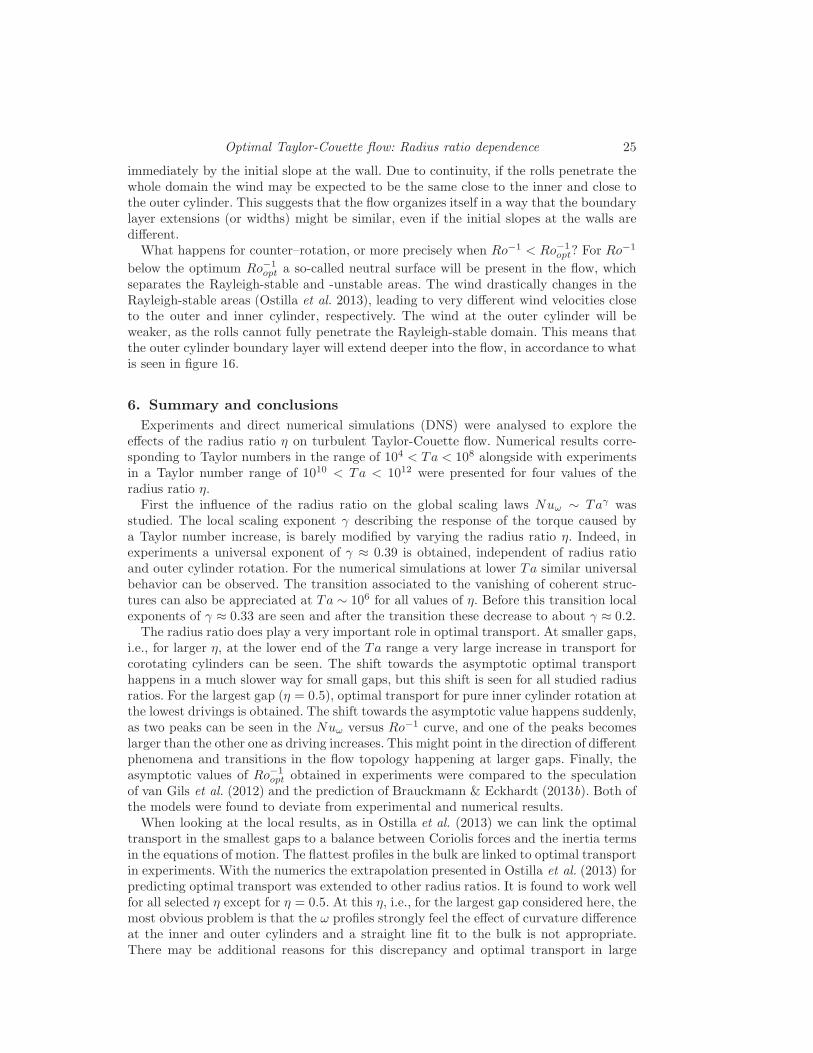
Optimal Taylor-Couette flow: Radius ratio dependence 25

immediately by the initial slope at the wall. Due to continuity, if the rolls penetrate thewhole domain the wind may be expected to be the same close to the inner and close tothe outer cylinder. This suggests that the flow organizes itself in a way that the boundarylayer extensions (or widths) might be similar, even if the initial slopes at the walls aredifferent.What happens for counter–rotation, or more precisely when Ro−1 < Ro−1

opt? For Ro−1

below the optimum Ro−1

opt a so-called neutral surface will be present in the flow, whichseparates the Rayleigh-stable and -unstable areas. The wind drastically changes in theRayleigh-stable areas (Ostilla et al. 2013), leading to very different wind velocities closeto the outer and inner cylinder, respectively. The wind at the outer cylinder will beweaker, as the rolls cannot fully penetrate the Rayleigh-stable domain. This means thatthe outer cylinder boundary layer will extend deeper into the flow, in accordance to whatis seen in figure 16.

6. Summary and conclusions

Experiments and direct numerical simulations (DNS) were analysed to explore theeffects of the radius ratio η on turbulent Taylor-Couette flow. Numerical results corre-sponding to Taylor numbers in the range of 104 < Ta < 108 alongside with experimentsin a Taylor number range of 1010 < Ta < 1012 were presented for four values of theradius ratio η.First the influence of the radius ratio on the global scaling laws Nuω ∼ Taγ was

studied. The local scaling exponent γ describing the response of the torque caused bya Taylor number increase, is barely modified by varying the radius ratio η. Indeed, inexperiments a universal exponent of γ ≈ 0.39 is obtained, independent of radius ratioand outer cylinder rotation. For the numerical simulations at lower Ta similar universalbehavior can be observed. The transition associated to the vanishing of coherent struc-tures can also be appreciated at Ta ∼ 106 for all values of η. Before this transition localexponents of γ ≈ 0.33 are seen and after the transition these decrease to about γ ≈ 0.2.The radius ratio does play a very important role in optimal transport. At smaller gaps,

i.e., for larger η, at the lower end of the Ta range a very large increase in transport forcorotating cylinders can be seen. The shift towards the asymptotic optimal transporthappens in a much slower way for small gaps, but this shift is seen for all studied radiusratios. For the largest gap (η = 0.5), optimal transport for pure inner cylinder rotation atthe lowest drivings is obtained. The shift towards the asymptotic value happens suddenly,as two peaks can be seen in the Nuω versus Ro−1 curve, and one of the peaks becomeslarger than the other one as driving increases. This might point in the direction of differentphenomena and transitions in the flow topology happening at larger gaps. Finally, theasymptotic values of Ro−1

opt obtained in experiments were compared to the speculationof van Gils et al. (2012) and the prediction of Brauckmann & Eckhardt (2013b). Both ofthe models were found to deviate from experimental and numerical results.When looking at the local results, as in Ostilla et al. (2013) we can link the optimal

transport in the smallest gaps to a balance between Coriolis forces and the inertia termsin the equations of motion. The flattest profiles in the bulk are linked to optimal transportin experiments. With the numerics the extrapolation presented in Ostilla et al. (2013) forpredicting optimal transport was extended to other radius ratios. It is found to work wellfor all selected η except for η = 0.5. At this η, i.e., for the largest gap considered here, themost obvious problem is that the ω profiles strongly feel the effect of curvature differenceat the inner and outer cylinders and a straight line fit to the bulk is not appropriate.There may be additional reasons for this discrepancy and optimal transport in large

26 R. Ostilla Monico and others

Radius ratio (η) Ro−1

opt/aopt from extrapolation Measured Ro−1

opt/aopt

0.5 -0.33/0.20 -/-0.714 -0.20/0.33 -0.20/0.330.769 -/- -0.20/0.360.833 -0.12/0.41 -0.10/0.370.909 -0.05/0.34 -0.05/0.34

Table 2: Summary of values obtained for Ro−1

opt and aopt through both the extrapolationof d〈ω〉z/dr (Section 5.2) and direct measurement of the torque (Section 4.2) for thevarious values of η studied in this paper.

gaps requires more investigation. A summary of the results for determining Ro−1

opt usingboth the experimentally measured torque maxima from section 4.2 and the numericalextrapolation from section 5.2 are presented in table 2.Finally, the boundary layers have been analyzed. The outer boundary layer is found to

be much thicker than the inner boundary layer when Ro−1 < Ro−1

opt. We attribute this tothe appearance of Rayleigh-stable zones in the flow. This prevents the turbulent Taylorvortices from covering the full domain between the cylinders. As the boundary layer sizeis essentially determined by the wind, if the rolls penetrate the whole domain (which isthe case for Ro−1 > Ro−1

opt), both boundary layers are approximately of the same size. Ifthe rolls do not penetrate the full domain, the outer boundary layer will be much largerthan the inner boundary layer, in accordance with the smaller initial slope of ω(r) at thecylinder walls.In this work, simulations and experiments have been performed on a range of radius

ratios between 0.5 6 η 6 0.909. Insights for the small gaps seem to be consistent withwhat was discussed in Ostilla et al. (2013). However, for η = 0.5 the phenomena ofoptimal transport appears to be quite different. Therefore, our ambition is to extend theDNS towards values of η smaller than 0.5 to improve the understanding of that regime.Acknowledgements: We would like to thank H. Brauckmann, B. Eckhardt, S. Mer-

bold, M. Salewski, E. P. van der Poel and R. C. A. van der Veen for various stimulatingdiscussions during these years, and G.W. Bruggert, M. Bos and B. Benschop for tech-nical support. We acknowledge that the numerical results of this research have beenachieved using the PRACE-2IP project (FP7 RI-283493) resource VIP based in Ger-many at Garching. We would also like to thank the Dutch Supercomputing ConsortiumSurfSARA for technical support and computing resources. We would like to thank FOM,the Simon Stevin Prize of the Technology Foundation STW of The Netherlands, COSTfrom the EU and ERC for financial support through an Advanced Grant.

REFERENCES

Ahlers, G. 1974 Low temperature studies of the Rayleigh-Benard instability and turbulence.Phys. Rev. Lett. 33, 1185–1188.

Ahlers, G., Grossmann, S. & Lohse, D. 2009 Heat transfer and large scale dynamics inturbulent Rayleigh-Benard convection. Rev. Mod. Phys. 81, 503.

Andereck, C. D., Liu, S. S. & Swinney, H. L. 1986 Flow regimes in a circular couette systemwith independently rotating cylinders. J. Fluid Mech. 164, 155.

Behringer, R. P. 1985 Rayleigh-Benard convection and turbulence in liquid-helium. Rev. Mod.Phys. 57, 657 – 687.

Benjamin, T. B. 1978 Bifurcation phenomena in steady flows of a viscous liquid. Proc. R. Soc.London A 359, 1–43.

Optimal Taylor-Couette flow: Radius ratio dependence 27

Bodenschatz, E., Pesch, W. & Ahlers, G. 2000 Recent developments in Rayleigh-Benardconvection. Ann. Rev. Fluid Mech. 32, 709–778.

Brauckmann, H. & Eckhardt, B. 2013a Direct numerical simulations of local and globaltorque in Taylor-Couette flow up to Re=30.000. J. Fluid Mech. 718, 398–427.

Brauckmann, H. & Eckhardt, B. 2013b Intermittent boundary layers and torque maximain Taylor-Couette flow. Phys. Rev. E 87, 033004.

Busse, F. H. 1967 The stability of finite amplitude cellular convection and its relation to anextremum principle. J. Fluid Mech. 30, 625–649.

Chandrasekhar, S. 1981 Hydrodynamic and Hydromagnetic Stability . New York: Dover.

Couette, M. 1890 Etudes sur le frottement des liquides. Gauthier-Villars et fils.

Coughlin, K. & Marcus, P. S. 1996 Turbulent bursts in Couette-Taylor flow. Phys. Rev. Lett.77 (11), 2214–17.

Cross, M. C. & Hohenberg, P. C. 1993 Pattern formation outside of equilibrium. Rev. Mod.Phys. 65 (3), 851.

Dominguez-Lerma, M. A., Cannell, D. S. & Ahlers, G. 1986 Eckhaus boundary andwavenumber selection in rotating Couette-Taylor flow. Phys. Rev. A 34, 4956.

Dong, S 2007 Direct numerical simulation of turbulent taylor-couette flow. J. Fluid Mech. 587,373–393.

Dong, S 2008 Turbulent flow between counter-rotating concentric cylinders: a direct numericalsimulation study. J. Fluid Mech. 615, 371–399.

Donnelly, R. 1991 Taylor-Couette flow: the early days. Physics Today pp. 32–39.

Drazin, P.G. & Reid, W. H. 1981 Hydrodynamic stability . Cambridge: Cambridge UniversityPress.

Eckhardt, B., Schneider, T.M., Hof, B. & Westerweel, J. 2007 Turbulence transitionin pipe flow. Annu. Rev. Fluid Mech. 39, 447–468.

Esser, A. & Grossmann, S. 1996 Analytic expression for Taylor-Couette stability boundary.Phys. Fluids 8, 1814–1819.

Fasel, H. & Booz, O. 1984 Numerical investigation of supercritical taylor-vortex flow for awide gap. J. Fluid Mech. 138, 21–52.

Gebhardt, Th. & Grossmann, S. 1993 The Taylor-Couette eigenvalue problem with inde-pendently rotating cylinders. Z. Phys. B 90 (4), 475–490.

van Gils, D. P. M., Bruggert, G. W., Lathrop, D. P., Sun, C. & Lohse, D. 2011a TheTwente Turbulent Taylor-Couette (T 3C) facility: strongly turbulent (multi-phase) flowbetween independently rotating cylinders. Rev. Sci. Instr. 82, 025105.

van Gils, D. P. M., Huisman, S. G., Bruggert, G. W., Sun, C. & Lohse, D. 2011b Torquescaling in turbulent Taylor-Couette flow with co- and counter-rotating cylinders. Phys. Rev.Lett. 106, 024502.

van Gils, D. P. M., Huisman, S. G., Grossmann, S., Sun, C. & Lohse, D. 2012 OptimalTaylor-Couette turbulence. J. Fluid Mech. 706, 118.

Grossmann, S. & Lohse, D. 2000 Scaling in thermal convection: A unifying view. J. Fluid.Mech. 407, 27–56.

Grossmann, S. & Lohse, D. 2001 Thermal convection for large Prandtl number. Phys. Rev.Lett. 86, 3316–3319.

Grossmann, S. & Lohse, D. 2011 Multiple scaling in the ultimate regime of thermal convection.Phys. Fluids 23, 045108.

Grossmann, S. & Lohse, D. 2012 Logarithmic temperature profiles in the ultimate regime ofthermal convection. Phys. Fluids 24, 125103.

Huisman, S.G., van Gils, D.P.M. & Sun, C. 2012a Applying laser doppler anemometry insidea taylor-couette geometry – using a ray-tracer to correct for curvature effects. Eur. J. Mech.- B/Fluids 36, 115–119.

Huisman, S. G., van Gils, D. P. M., Grossmann, S., Sun, C. & Lohse, D. 2012b Ultimateturbulent Taylor-Couette flow. Phys. Rev. Lett. 108, 024501.

Huisman, S. G., Scharnowski, S., Cierpka, C., Kaehler, C., Lohse, D. & Sun, C. 2013Logarithmic boundary layers in highly turbulent Taylor-Couette flow. Phys. Rev. Lett 110,264501.

Kadanoff, L. P. 2001 Turbulent heat flow: Structures and scaling. Phys. Today 54 (8), 34–39.

28 R. Ostilla Monico and others

Lathrop, D. P., Fineberg, Jay & Swinney, H. S. 1992a Transition to shear-driven turbulencein Couette-Taylor flow. Phys. Rev. A 46, 6390–6405.

Lathrop, D. P., Fineberg, Jay & Swinney, H. S. 1992b Turbulent flow between concentricrotating cylinders at large Reynolds numbers. Phys. Rev. Lett. 68, 1515–1518.

Lewis, G. S. & Swinney, H. L. 1999 Velocity structure functions, scaling, and transitions inhigh-Reynolds-number Couette-Taylor flow. Phys. Rev. E 59, 5457–5467.

Lohse, D. & Xia, K.-Q. 2010 Small-scale properties of turbulent Rayleigh-Benard convection.Ann. Rev. Fluid Mech. 42, 335–364.

Lorenz, E. N. 1963 Deterministic nonperiodic flow. J. Atmos. Sci 20, 130–141.Mallock, A. 1896 Experiments on fluid viscosity. Phil. Trans. R. Soc. Lond. A 187, 41–56.Merbold, S., Brauckmann, H. & Egbers, C. 2013 Torque measurements and numerical

determination in differentially rotating wide gap Taylor-Couette flow. Phys. Rev. E 87,023014.

Ostilla, R., Stevens, R. J. A. M., Grossmann, S., Verzicco, R. & Lohse, D. 2013Optimal Taylor-Couette flow: direct numerical simulations. J. Fluid Mech. 719, 14–46.

Ostilla Monico, R., van der Poel, E., Verzicco, R., Grossmann, S. & Lohse, D. 2013Boundary layer dynamics at the transition between the classical and the ultimate regimeof Taylor-Couette flow. submitted to Physics of Fluids .

Paoletti, M. S. & Lathrop, D. P. 2011 Angular momentum transport in turbulent flowbetween independently rotating cylinders. Phys. Rev. Lett. 106, 024501.

Pfister, G. & Rehberg, I. 1981 Space dependent order parameter in circular Couette flowtransitions. Phys. Lett. 83, 19–22.

Pfister, G, Schmidt, H, Cliffe, K A & Mullin, T 1988 Bifurcation phenomena in Taylor-Couette flow in a very short annulus. J. Fluid Mech. 191, 1–18.

Pirro, Davide & Quadrio, Maurizio 2008 Direct numerical simulation of turbulent Taylor-Couette flow. Eur. J. Mech. B-Fluids 27, 552.

Siggia, E. D. 1994 High Rayleigh number convection. Annu. Rev. Fluid Mech. 26, 137–168.Smith, G. P. & Townsend, A. A. 1982 Turbulent Couette flow between concentric cylinders

at large Taylor numbers. J. Fluid Mech. 123, 187–217.Stevens, R. J. A. M., Lohse, D. & Verzicco, R. 2011 Prandtl and Rayleigh number depen-

dence of heat transport in high Rayleigh number thermal convection. J. Fluid Mech. 688,31–43, submitted.

Stevens, R. J. A. M., Verzicco, R. & Lohse, D. 2010 Radial boundary layer structure andNusselt number in Rayleigh-Benard convection. J. Fluid Mech. 643, 495–507.

Strogatz, S. H. 1994 Nonlinear dynamics and chaos. Reading: Perseus Press.Swinney, H. L. & Gollub, J. P. 1981 Hydrodynamic instabilities and the transition to turbu-

lence, , vol. 45 (Topics in Applied Physics). Berlin: Springer-Verlag.Taylor, G. I. 1936 Fluid friction between rotating cylinders. Proc. R. Soc. London A 157,

546–564.Tong, P., Goldburg, W. I., Huang, J. S. & Witten, T. A. 1990 Anisotropy in turbulent

drag reduction. Phys. Rev. Lett. 65, 2780–2783.Verzicco, R. & Orlandi, P. 1996 A finite-difference scheme for three-dimensional incom-

pressible flow in cylindrical coordinates. J. Comput. Phys. 123, 402–413.Wendt, F. 1933 Turbulente Stromungen zwischen zwei rotierenden Zylindern. Ingenieurs-

Archiv 4, 577–595.Xia, K.-Q., Lam, S. & Zhou, S. Q. 2002 Heat-flux measurement in high-Prandtl-number

turbulent Rayleigh-Benard convection. Phys. Rev. Lett. 88, 064501.