Optimal Speed of Transition 10 Years After - Weeblyekonomiks.weebly.com/uploads/5/5/1/5/5515573/boeri_2000_optim… · Optimal Speed of Transition 10 Years After ... expected outcomes

Optimal Speed of Transition 10 Years After

by Tito Boeri, IGIER and CEPR

1. Introduction

When the transition was started there was no historical precedent to draw upon while makinginferences on the future course of events. Educated guesses were allowed and were made, quitemany of which turned out subsequently to be wrong. Knowledge evolves by comparing actual withexpected outcomes and learning from these deviations. It is easy to be wise after the events. It ismore difficult to understand why wrong predictions were made at the outset. This is the primarygoal of this paper. From these predictions, the common wisdom prevailing at the beginning of the1990s we need, in any event, to start.

There were three common predictions made at the outset of transition.

First, the removal of state subsidies and associated hardening of budget constraints would forcemany state enterprises to close down, inducing large scale labour shedding. In order to restructurethese firms, rather than simply close down the shop, it was essential to win the strong resistance ofworkers to change, that is, to “buy them off”.

Second, as a result of this shake-out striking at the core of “socialist employment”, large inflowsinto unemployment of redundant workers would have to be expected. As the size of these inflowswas related to the pace of closure of state enterprises, it was also argued that unemployment couldbe considered as an indicator of the determinacy of government to push through reforms andimpose tough budget constraints on enterprises.

Third, unemployment would gradually be absorbed by the growth of the emerging sectors, namelyprivate firms, mainly clustered in retail trade, the service sector or in light, final consumption goods,industries artificially compressed by central planning emphasis on primary accumulation.

In a nutshell, labour reallocation was deemed to occur mainly through unemployment, the singlemost important indicator of the speed of transition trajectories.

From a normative point of view, a careful timing of reforms was called for. Most of the modelsused to speculate on the future course of events yielded a multiplicity of equilibria and a non-trivialrelation between the speed and final outcomes of transition. On the one hand, reforms had to beenforced in such a way as to avoid creating too much unemployment before a critical size of theprivate sector had been reached. Otherwise, social unrest related to increasing unemployment and

2

the associated political backlashes of reformers, the fiscal burden induced by unemployment benefitpayments or other “feedback” mechanisms (e.g., income effects of dis-employment) would blockreforms. On the other hand, reforms could not be too slow as resources had to be freed for thegrowth of the private sector, unemployment had to start exerting its moderating effects on wageclaims (and employers were deemed not sufficiently organised to resist such claims) and increasedproductivity had to stimulate investment. This was the essence of the trade-offs entailed by themodels of the speed of transition developed at early stages of the process and widely used in policyadvice throughout the region.

In this paper we will start by reviewing the extensive literature on the optimal speed of transition.Next, we will assess the empirical relevance and predictive accuracy of these models based oninformation on aggregate stocks and flows. The final section of this paper will list the variouspieces of evidence left unexplained by this rich (and still flourishing) literature and argue thatsolving these puzzles is important in the light of the challenges facing these countries in the years tocome. Thus, we will start by the theory and then go to the facts. The reader knowing the optimalspeed literature can skip section 1.2 and go directly to the evidence presented in section 1.3.

2. What did we expect to occur?

When I first visited Warsaw at the beginning of January 1990, the policy-makers I met were largelyunderestimating the growth of unemployment. I distinctly remember that their estimates rangedfrom 50,000 (according to the most optimistic views, shared, inter alia, by the first Labour Ministerof the new Poland) to 200,000 unemployed. Needless to say, at the end of that month, there werealready 56,000 people registered unemployed in the Polish labour offices and the “pessimistic”200,000 threshold was attained after just two months. One year later there were 1.2 millionindividuals registered unemployed. One-and-a-half years later the 2 million threshold had beencrossed. Four years later about 3 million Polish citizens were registered as unemployed at labouroffices.

The climate in the international organisations and within the scientific community was verydifferent. The cross-country comparative view organisations like the IMF, OECD and World Bank,could draw upon and perhaps also the “distance” from which they could observe developments inthe transition world dictated much less optimistic views as to the likely rise and magnitude of“transitional unemployment”. The experience of eastern Germany was, after all, emblematic. Evenif eastern German unemployment had been to a large extent a by-product of the political decision tofix a 1-to-1 parity of the eastern mark to the DM (and of the extension to the East of the westernsystem of industrial relations1), these large cohorts of jobseekers were coming from enterprisesoften generating negative value-added and this evidence was even more striking as coming from thetechnological leader of the former CMEA (Council for Mutual Economic Assistance) block. Thus,there were many Cassandras around and ….I was among them.

Not only was unemployment considered inevitable, but it was also deemed to be an indicator of thespeed of transition2. To a common way of thinking, there was a simple mechanics of transition. Onthe one hand, the removal of subsidies to state enterprises and their exposure to market disciplinewould force the managers of these firms to shed labour. On the other hand, a flourishing private

1 According to von Hagen (1997), the fact of exporting to eastern Germany western-type collective bargaininginstitutions reduced the competitivity of new Länders even more seriously than the exchange rate established at the timeof unification.2 Cf. McAuley (1990).

3

sector would generate employment opportunities in the numerous market areas (e.g., retail trade)and niches (central planning did not allow for product differentiation satisfying consumers’preferences for variety) artificially compressed under the old system. Thus, inflows intounemployment coming from the downscaling of state enterprises and outflows from unemploymentassociated with the emergence of the private sector were expected with the former exceeding thelatter at earlier stages of transition because of the small scale of the private sector at the start of theprocess. Hence, unemployment would increase even if employment growth in the private sectorwas faster than job destruction in the state sector.

As an illustration of this scale effects, assume that a proportion “s” of employment in stateenterprises (Es) is shed per period whilst in the meantime the private sector (Ep) generates “g” newposts per any job existing at the beginning of the period. Thus, we have that:

( 1) ps EgEsOIU .. −=−=∆

From (1) it follows that unemployment inflows (I) can exceed unemployment outflows (O), henceunemployment can grow ( U∆ be positive) even if g is greater than s, insofar as Ep is smallcompared to Es.

Put another way, unemployment was unavoidable at early stages of transition because even abuoyant private sector could not compensate employment losses in the overmanned state enterprisesinherited from the previous system3. However, further down the transition path, i.e. for large Ep andsmall Es, unemployment would have to decline because the scale effects would begin to work theother way round. Overall, a hump-shaped dynamics of unemployment was expected, withunemployment initially increasing and then declining.

Unemployment was also deemed to be an indicator of the speed of reforms: inflows intounemployment were determined solely by the parameter “s”, capturing the pace of labour sheddingin state enterprises and hence the timing of removal of state subsidies and, more broadly, thetightening of the budget constraints of state enterprises.

Although unemployment was unavoidable, governments could at least prevent too large an initialrise in the number of jobless people, by fine-tuning employment reductions in state enterprises withthe absorption capacity of the emerging private sector. However, the slowing down of restructuringin state enterprises could negatively affect the development of the private sector, by preventingexcess labour from exerting downward pressure on wages and possibly via fiscal displacementeffects related to the financing of subsidies to state enterprises.

3 Several estimates were provided at the beginning of transition of the amount of “labour hoarding” (e.g., see OECD,1994), that is employment kept in excess of what needed to attain the targeted output level. Most of these estimateswere just guesses as there were no time-series of employment under different cyclical conditions or ad-hoc surveys todraw upon. The estimates pointed to overmanning accounting between 30 and 60 per cent of state sector employment atthe beginning of the 1990s. Interestingly, the reduction of labour hoarding was considered by many eastern economistsas the single most important sign of “marketisation” as if i) restructuring had involved only cost-minimisation, ii) firmsalso in the West, particularly in downturns, were not keeping workers in excess to the extent needed to reach a givenlevel of output, and iii) reducing overmanning could be always crucial, e.g., even in countries and time-periods whenreal wages were falling dramatically.

4

2.1. Fine-tuning the speed of transition

These interactions between “s” and “g”, and policy trade-offs between the tightening of the budgetconstraints of state enterprises, unemployment and the development of the private sector are at thecore of the theoretical literature on the optimal speed of transition (OST for short), which offeredrelevant background material for policy advice throughout the region. As the building blocks andmain implications of the various models are reviewed in the annex, we can confine ourselves hereinto summarising the key findings of this literature and the basic assumptions it relies upon.

A common feature of these models is the assumption that labour supply is fixed, i.e. persons areeither employed (E with the subscripts s and p denoting, respectively, state and private firms) orunemployed (U). In other words, labour market adjustment does not involve flows to and from out-of-the-labour force (OLF). Another key simplifying assumption is that flows from public sector toprivate sector employment are necessarily mediated by intervening unemployment spells, that is nodirect shift of workers from state to private enterprises occurs. The kind of flows allowed and“banned” under this literature are summarised in Figure 1.

This literature also considers the speed of closure of state sector jobs, labelled by s, as a controlvariable. Governments can affect labour shedding in state enterprises in various ways, e.g., bygranting them subsidies, and by imposing strict employment protection legislation (e.g., non-negligible severance and advance notification requirements on firms implementing layoffs). Theother key policy variable is the generosity of unemployment benefits (summarised by the ratio ofbenefits to the ongoing wage or “replacement rate”, b) provided to those displaced in transition.Governments can manipulate parameters “s” and “b” within their budget constraint. The latter isgenerally assumed to be static, that is, no deficit financing is allowed. Only the model by Coricelli(1996) allows for intertemporal budget constraints.

All these models aim at capturing institutional features of transitional economies, such as theimportant role played by workers in decision-making in state enterprises, and typically generateunemployment even at the steady state equilibrium. Although the micro-foundations of thesemodels are not spelled out, reference is occasionally made to two sources of involuntaryunemployment, namely the presence of moral hazard, e.g. associated with imperfect monitoring ofworkers’ effort, or adverse selection, e.g. because of poor signals as to workers’ actual productivity,both leading employers in the private sector to set wages above the market clearing level (efficiencywages). Frictions in the labour market making it more costly and time-consuming to reallocateworkers from the state sector to the private sector are also framed, notably in the models by Burda(1993) and Gavin (1993). Thus, the literature departs from the standard assumptions and the basicsetup of neoclassical growth theory. The price of this greater realism is that models are very rich instructural assumptions and it is more difficult to disentangle the role played by each marketimperfection and to identify what drives labour market dynamics. The OST literature also follows,more or less admittedly4, a partial equilibrium approach, the main exception being in this case thegeneral equilibrium model by Castanheira and Roland (1998) which is also an attempt to bridge thegap between these models and standard growth theory.

The policy trade-offs involved in the transition process are embedded in these models in a numberof feedback mechanisms: unemployment growth is, on the one hand, influenced by the speed of theremoval of state subsidies, but, on the other hand, high unemployment may strike back on speedbecause of fiscal effects related to the funding of unemployment benefits, political economy factorseroding the consensus gathered around the reform effort or other mechanisms. 4 Even if ad hoc assumptions allow some authors to claim that these are general equilibrium models, their setup is apartial equilibrium one.

5

In the seminal model by Aghion and Blanchard (1994) the basic feedback mechanism is onecoming from the fiscal side: high unemployment means large outlays to fund unemploymentbenefits (as supposedly subsidising overmanning in state enterprises is costless while paying peopleout of work is not5), hence higher payroll taxation. This in turn reduces job creation in the privatesector. This “fiscal externality” is at work also in the models by Burda (1993) and by Chadha andCoricelli (1994). The latter, unlike Aghion and Blanchard, allow for differential taxation of stateand private enterprises. In particular, effective tax rates are assumed to be higher in the state than inthe private sector owing to problems in revenue collection faced when dealing with private (andsmall) business. Hence, on Chadha and Coricelli’s model, the fiscal balance deteriorates in thetransition process even when unemployment is stable because an increasing proportion of the totalwage bill of the economy is being paid by private employers6.

Another class of models identifies potential feedback mechanisms in political economy factors7.This is the case of the frameworks proposed, inter alia, by Przeworski (1993), Rodrik (1995) andDewatripont and Roland (1992 and 1995). Rodrik’s model shows that the window of opportunitiesexisting at the outset of transition8 rapidly erodes as workers in state enterprises find it more andmore difficult to shift to the emerging private sector and hence vote against further cuts to subsidiesto state enterprises (which are, counterfactually, supposed to be entirely financed via taxation ofprivate enterprises). In Dewatripont and Roland (1992), a big-bang reform strategy is bound to bestopped under majority rule. The only way to enact reforms is to introduce them gradually usingdivide-and-rule tactics whereby only the workers hurt by each reform will oppose it9. Divide-and-rule tactics are also essential to start restructuring firms whose workers exert substantial controlover managerial decisions. Under these circumstances, a sharp initial rise of unemployment mayblock reforms. If unemployment increases too much at the outset of transition, workers will opposerestructuring as they face low re-employment probabilities in the case of job loss (Blanchard, 1997).Intuitively, the job finding probability is given by outflows from unemployment over theunemployment stock, and high unemployment means a large “denominator” per any givenabsorption capacity of the private sector, that is per any given numerator.

5 In this model subsidies to state enterprises come from Heaven. Subsidies to state enterprises are simply a policyinstrument governments can freely adjust – that is, without taking resources away from other public expenditure items -- in order to affect the speed of transition.6 The model by Castanheira and Roland (1998) does not have such a feedback mechanism. However, a too fast processof sectoral reallocation of workers can still end up perversely slowing down the transition process and generates massunemployment because the (negative) income effects associated with plant closures dominate the (positive) substitutioneffects of wage declines induced by increasing unemployment.7 To be fair, political economy considerations are present also in the model by Aghion and Blanchard (1994). Asspelled out in a subsequent work by Blanchard (1997), the generosity of unemployment benefits plays a key role inallowing worker-controlled state enterprises to begin (strategic) restructuring. However, the political economy ofreforms -- notably industrial relations within the enterprise -- matters in these models only insofar as it hastens orpostpones the restructuring of state enterprises. In other words, poltical economy factors do not play the role of afeedback mechanism potentially reversing the process once this has started.8 This window of opportunity is present also in the case of strategic voting when state enterprises are highly inefficientat the outset of transition. Even by initially voting against the reforms, state sector workers colud not prevent themedian voter (whose preferences ultimately drive policy decisions) from getting out of the state sector. Moreover, ifstate sector workers succeed in shifting to the private sector, they will have to bear the burden of the subsidy theyinitially voted for. As long as private sector workers and the unemployed always vote against the subsidy, however,strategic voting rules out the possibility of policy reversals.9 This applies also when workers are forward-looking provided that the “old” sectors (e.g., state enterprises and co-operatives) are bound to disappear at some finite date. This is not the case in some OST models. For instance, inRodrik’s (1995) model, the state sector is supposed to survive even at the steady state equilibrium in spite of persistentproductivity (and wage) differentials vis-à-vis the private sector.

6

The presence of such feedback mechanisms opens up the possibility of a multiplicity of equilibria.This may be a desirable property of these models insofar as they aim also at explaining cross-country differences in the levels at which unemployment is stabilising throughout central andeastern Europe and the former Soviet Republics. For instance, in Aghion and Blanchard’s (1994)model, depending on the expectations of private sector employers, the economy may end up at alow unemployment equilibrium or the transition may fail, leading the economy to be trapped in ahigh unemployment equilibrium. Expectations matter because private employers decide on hiringson the basis of their assessment of their lifetime tax liabilities. Expectations are self-fulfilling aspessimistic private employers end up paying more taxes: they absorb workers shed by stateenterprises too slowly, and hence have to pay more for unemployment benefits. A credible10

commitment by governments to reduce unemployment benefits (or to slow down restructuring instate enterprises) when unemployment is too high can prevent the occurrence of the highunemployment equilibrium.

2.2. Policy implications of the OST literature

Multiple equilibria and non-linearities in the adjustment paths point to the role of economic policiesin ruling out “bad” equilibria11, easing transition and reducing the risk of derailments. Thus, theOST literature has relevant policy implications as to i) the magnitude and timing of reduction ofsubsidies to state enterprises, ii) the generosity of unemployment benefits, iii) the form and speed ofprivatisation, and iv) the scope for deficit financing of social policies in the course of transition.

Although all models imply that subsidies to state enterprises will sooner or later have to be lifted,the OST literature suggests that there is a careful timing to be followed in the tightening of thebudget constraints of state enterprises: too quick a reduction of subsidies means too large an initialrise of unemployment and associated fiscal burden (and/or income effects), hindering the growth ofthe private sector. Hence, subsidies have some role to play at the outset of transition. In otherwords, the OST literature makes a case for gradualism in spite of the fact that two key factorsgenerally moving the balance in favour of gradualism vs. big-bang12 – the presence of a politicallearning process, and the possibility of early reversals -- are not embedded in these models.

Unemployment benefits play a twofold role in these models. On the one hand, insofar as theyincrease the value of the outside option of state sector workers, they ease13 the restructuring of stateenterprises by reducing the opposition of insiders to employment reductions and to privatisation.On the other hand, the financing of unemployment benefits puts a brake on private employmentcreation and hence reduces its capacity to absorb labour shed from state enterprises. Owing to thistrade-off between the effects of benefits on restructuring and on private job creation, unemploymentbenefits should be rather generous at the start of transition and then reduced (actually, in order to

10 The announcement that benefits will be reduced if unemployment becomes too high may not be credible ex-ante.However, governments in the region proved capable of significantly tightening up unemployment benefits whenunemployment was at its transitional peaks.11 High and low unemployment need not necessarily be synonymous in these models with “good” and “bad” equilibria,respectively. For example, in the model by Chadha et al. (1993), the economy may get trapped in a low unemploymentequilibrium dominated by state firms, where no accumulation of physical and human capital takes place.12 The literature on gradualism vs. big-bang is reviewed in Dewatripont and Roland (1997).13 However, higher unemployment benefits negatively affect job finding probabilities of the unemployed by putting ahigher floor to wage bargaining in the private sector, which means lower job creation. If individuals place a relativelyhigh value on future consumption (if they have a rather low discount rate), the negative effect of higher benefits onunemployment outflows may offset the positive effect on the instantaneous value of being unemployed. See Annex 1for a characterisation of these two mutually offsetting effects.

7

rule out bad equilibria, governments should from the beginning commit themselves to reducebenefits if unemployment reaches a certain threshold). As shown by Blanchard (1997), later on,when unemployment is large, the “fiscal externality” tends to dominate. At that stage, a case forhigh benefits can only be made on equity grounds. This holds even when unemployment benefitsare also meant to promote better matches between jobseekers and vacancies. Insofar as individualsare not very risk-adverse (hence the provision of insurance does not significantly affect voluntarydecisions to undertake risky job search) and have a large precautionary demand for savings, alsounemployment benefits aimed at promoting better matches ultimately slow down restructuring[Atkeson and Kehoe, 1993].

The choice among different privatisation rules is framed in these models as a change in theproportion of post-privatisation profits going to insiders [Aghion and Blanchard, 1996], which iszero in the case of pure outsider privatisation. More generous privatisation rules (an insider shareclose to one unit) reduce the opposition of insiders to restructuring by increasing the benefits theycan get if they do not lose their job in the process. Unlike unemployment benefits, insiderprivatisation rules do not involve fiscal externalities (do not increase taxes paid by privateenterprises), and hence do not exert negative feedback effects on the reallocation process. Moreimportant still, insider privatisation tends to reduce wage claims in the private sector -- as nowworkers involved in privatisation receive a share of firms’ profits -- and may stimulate jobcreation14. Hence, these models generally argue in favour of insider privatisation, a case againstthis method being made mainly on distributional grounds (as insider privatisation makes everybodyworse off except those who happen to be employed in privatised firms).

Finally, debt-financing of social insurance is generally advocated by these models insofar as itallows offsetting of the feedback effects associated with the initial rise of unemployment.Excessively strict borrowing constraints – e.g., established in the context of macroeconomicstabilisation packages – may therefore have a negative effect on the pace of job reallocation andeven jeopardise the success of economic transformation [Chadha and Coricelli, 1994]. Yet, thekind of foreign borrowing which is allowed in these models is a foreign transfer not involvingfuture repayment obligations: more than foreign borrowing, it should be called a gift aimed atoffsetting the fiscal externality effects associated with the rise of unemployment.

Summarising, a key assumption of the OST literature is that labour supply is fixed: one can beeither employed or seeking a job. Inactivity is banned. In the light of this assumption, the manyvariants of the basic Harris-Todaro-type model which have been developed by this literature allconsider the rate of decline of state sector jobs, s, as something that can be altered at will bygovernments. The control over s is both direct – insofar as governments decide upon the amount ofsubsidies to be granted to state enterprises – and indirect – because workers controlling stateenterprises can be induced to accept restructuring plans by more generous unemployment benefits.Unemployment benefits themselves should be relatively generous at the start of transition, in orderto set in motion the reallocation process, but governments should be committed to reduce thegenerosity of benefits when unemployment is above a certain threshold. Because of the heavyfiscal burden imposed by the financing of these benefits on private job creation, employers need tobe convinced that transition will not eventually derail.

14 These models underplay (if they at all consider them) the effects of different privatisation rules on enterprisebehaviour via changes in corporate governance and managerial incentives. Hence, they neglect a possible feedbackeffect of insider privatisation on restructuring.

8

3. What Happened?

3.1. The output collapse

All transition countries experienced after the beginning of the systemic transformation one of thedeepest depressions ever observed in modern history. In the first two years of transition, GDPdeclined between 15 and 20 per cent (Figure 2., top panel). Output declines affected all sectors, butwere particularly marked in industry. Gross industrial production fell everywhere more sharplythan output and in Bulgaria and Romania industrial output halved between 1990 and 1992. The“transitional recession” was not less dramatic than the Great Depression. Actually, output declineswere sharper and, at least for the Commonwealth of Independent States (CIS) countries, moreprotracted than in the US in the 1930s (Figure 2, bottom panel).

The transitional recession is often characterised as a U-shaped evolution of output. However, this istrue only for the Central European countries, and yet some of them were at the end of 1998 stilllagging behind the GDP levels of the previous decade. Eastern Europe, after a short recovery,experienced a new marked decline of GDP six to eight years down the road of transition. In theCIS countries the recession had not reached an end eight years after the beginning of the systemictransformation. Acknowledging measurement errors in economies largely de-monetised like thoseof the CIS, recorded GDP levels in this region were in 1998 still at about 50 per cent of the pre-transition levels and the letter which could best describe the evolution of output is a L rather than aU.

The OST literature did not predict such a marked decline of output. And, after all, there was noreason to believe, a priori, that the transition from a less efficient to a more efficient productionsystem should have involved dramatic falls in output. Also from an empirical standpoint, labourand capital reallocation costs involved by structural change could not be expected a priori togenerate sizeable output losses. The empirical relation between structural change and outputobserved in OECD countries – the so-called Lilien’s hypothesis15 – cannot yield comparable falls inoutput and output losses were, in any event, initially uniform across the board.

While a number of statistical issues (some over-reporting of output under the previous regime,changes in the composition of output and in the availability of goods to consumers that may not becaptured by official statistics, a large hidden economy, etc.) could contribute to explain some of theGDP decline, the size of output losses could by no means reflect mere measurement problems.

Some explanations for the output losses were only provided ex-post – externally with respect to theOST literature16 -- and were, for the most, not entirely convincing. The most ingeniousinterpretation is that provided Blanchard and Kremer (1997). They point to the dis-organisation inthe production network, notably in the provision of materials and intermediate inputs, associatedwith the removal of central planning, the unbundling of the vertically integrated conglomeratesinherited from the previous regime and rent-seeking behaviour on the part of input providers assoon as the coercive power of central planning (in enforcing the production and delivery ofintermediate goods) ceased to exist. Under asymmetric information as to the reservation price ofinput providers or incomplete contracts, bargaining over input provision is inefficient and may lead

15 Cf. Lilien (1982).16 The only explanation for the output fall provided within the OST literature is associated with the work of Atkesonand Kehoe (1995) who point to labour market frictions associated with sectoral shifts. Yet output fall was experiencedunformly across the board and preceded sectoral shifts in employment. For earlier explanations of the output fall, seeGomulka (1992), Kornai (1993) and Wei Li (1994).

9

to a collapse of production in the state sector. At any stage along the chain of production, the inputprovider may indeed find it more advantageous to break the chain. These problems arising from theinterlocking of firms along the vertical links of production are bound to become less and lessimportant as transition proceeds insofar as rents induce the multiplication of suppliers and hence thefirm uphill in the production chain can always shift supplier. Thus, this explanation can only holdfor the initial stages of transition. Based on measures of the “complexity of production” (capturingthe number of intermediate inputs required by final goods in any given sector) obtained from input-output tables as well as business surveys reporting shortages of materials and intermediate inputs,Blanchard and Kremer find some support for the theory in Eastern Europe and the CIS17. Needlessto say, in these countries output falls were much more protracted than implied by a transient dis-organisational shock. Moreover Blanchard and Kremer’s model is based on two key assumption forwhich there still little, if any, empirical support: the presence of Leontief-type technologies, that is,technologies not allowing to replace inputs being temporarily under-provided and a markedspecificity of the inputs required by the firms inherited from the previous regime. Especially thelatter assumption may sound somewhat unrealistic for firms which were frequently subject underthe previous system to input shortages and in a context where production was still largely involvinghomogeneous goods and using inputs which were much less specific or specialised that in marketeconomies. Surveys of enterprises carried out in these countries suggest that mainly new firms,producing new products find it difficult to secure domestically an adequate provision ofintermediate goods and often have to use imported inputs18.

The explanation for the output fall provided by Roland and Verdier (1997) differs only slightlyfrom that of Blanchard and Kremer. Unlike the latter, Roland and Verdier emphasise the existenceof frictions in the search of new partners down the chain of production and relation-specificinvestment: firms do not invest until a long-term partner has not been found. Thus output fall intheir model arises not only because of the disruption of previous production links, but also becauseof a fall in investment and the depreciation of capital associated with the absence of replacementinvestment. Many of the points made concerning the empirical relevance of Blanchard andKremer’s apply also to this model.

3.2. Behind the stocks

For quite some time labour market developments in these countries seemed to closely conform to apriori expectations and to the predictions of the models summarised in the previous section.Employment in state enterprises was plummeting, unemployment skyrocketing and privateemployment growing rapidly. Projecting over time the monthly growth rates of public and privateemployment experienced in 1989-91 by Poland – the first country to embark on a comprehensivestructural transformation cum stabilisation process – and imposing, as customary in the OSTliterature, a constant labour force, one obtains the bell-shaped pattern of unemployment displayed inFigure 3, which bears a close resemblance to the evolutions implied by the models reviewed in theprevious section. Unemployment is initially rising, reaches two-digits levels and then in vanishesas quickly as it appeared: we have the predicted (and quite reassuring) bell-shaped evolution ofunemployment. Everything seemed to be working in line with expectations.

17 Based on data from enterprise surveys in the Ukraine and Russia Konings and Walsh (1999) found little support tothe role played by dis-organisation in the output fall in these two countries.18 See Koenings and Walsh (1999).

10

However, a closer scrutiny of labour market dynamics and access to flow data soon revealed [Boeri,1994] that the adjustment of labour markets in CEE was very different from what was predicted bythese models and anticipated in most policy fora and academic discussions.

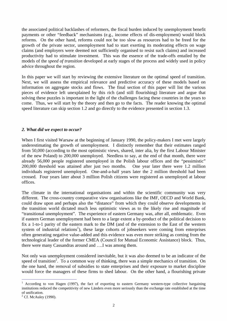
While employment reductions were expected to be driven by layoffs, data on separations from stateenterprises indicate that a significant component of outflows from state sector jobs was associatedwith voluntary quits. Available evidence from Labour Force Survey (LFS) data (reported in the toppanel of Table 1), points to rather large ratios of job leavers (persons currently non-employedbecause they had quit their previous job) to total employment and to shares of job losers (personscurrently non-employed because they were laid-off from their previous job) roughly comparable tothose observed in the European Union. Quite strikingly, in Poland and the Czech Republic theratio of job losers to total employment was even lower than in Italy, the OECD country located atthe top of rankings of employment protection against dismissals19 and experiencing among thelowest layoff rates in Western Europe. It should be stressed that the LFS questionnaire asks aboutthe nature of the separation only those currently non-employed and many quits are likely to end upin the take-up of another job rather than in non-employment. Hence the data reported in Table 1.are likely to significantly underestimate the proportion of quits in the total number of separations.

Disentangling quits from layoffs on the basis of administrative data is notoriously difficult as oftenseparations classified as under “mutual” agreements may hide actual layoffs. The abovenotwithstanding, data from the unemployment registers (reported in the bottom panel of Table 1),which also have the advantage of covering the very beginning of the transition process, suggest thatthe bulk of flows from employment to unemployment in 1991-2 was indeed represented by quits.Relatively many voluntary separations were also observed in countries which embarked later upona structural transformation process, such as Russia. Based on an enterprise survey carried out bythe World Bank, Commander et al. (1995) report that only about 25 per cent of separations fromstate enterprises in Russia were associated with individual or collective layoffs.

Information from the registers of jobseekers pointed to monthly inflow rates into unemployment(unemployment inflows as a proportion of the working age population) of half a percentage point inmost transition countries [OECD, 1994b], compared with above one per cent in western Europe and2-3 per cent in North America. Thus, unemployment was rising not because of the predicted largecohorts of workers being laid-off from state enterprises, but as a result of remarkably low outflowrates. Outflows from unemployment to jobs, in particular, were marginal. With the notableexception of the Czech Republic, only up to five out of one hundred jobseekers were leavingunemployment every month because they had found a job. When using administrative records (datafrom the unemployment register), outflows to jobs generally offer a better measure of actual exitsfrom unemployment than total outflows. This is because exits from the unemployment registers notassociated with the take-up of a job are often merely a by-product of the exhaustion of themaximum duration of benefits20. Thus, outflow to job rates of the order of 5 per cent implied that –had unemployment stabilised at these levels – the average duration of unemployment would havebeen of the order of 20 months!

Finally, contrary to popular wisdom and the transition mechanics embedded in the models reviewedabove, the ownership of enterprises did not discriminate between job creation and destruction. Thebulk of net job creation was concentrated in self-employment and the new small business sector.Enterprises being privatised did not seem to behave very differently from enterprises still in state

19 See OECD (1994a).20 This comes out very clearly when inspecting data from the Hungarian labour offices. There is almost a one-to-onecorrespondence between unemployment benefit receipt and registration at labour office for those who cannot claimsocial assistance (e.g., because they do not pass a means test) [Boeri and Pulay, 1998].

11

hands, in terms of both employment and output performance [Bilsen and Könings, 1998; Könings,Lehmann and Schaffer, 1996; Richter and Schaffer, 1996] and employment-output elasticities in(large) private enterprises were comparable to those observed in the units still in state hands [Estrinand Svejnar, 1998].

Hence, while the stocks seemed to behave as anticipated, for labour market flows it was a differentstory. And quite a different one.

The differences between actual labour market flows and their characterisation under the OSTliterature can be highlighted by matched records across household surveys. By tracking the sameindividual over different LFS waves, it is possible to map transitions from one state in the labourmarket to another21. LFS data are based on a similar methodology and harmonised questionnairesacross Europe, hence offering a better basis than data from the unemployment registers for cross-country comparisons. Unfortunately, transition countries started carrying out such surveys onlythree to five-six years down the road of transition22, which means that available data cannot capturethe early stages of transition.

With the above caveats in mind, Figure 4. characterises yearly transition probabilities (gross flowsover the base-year stock of origin), estimated on the basis of the LFS carried out in Poland, the firstcountry in the region to have introduced such a survey, in 1992-3. Similar patterns emerge bymatching records across LFS waves in other Central European countries, such as the Czech andSlovak Republics and Hungary (Boeri and Bruno, 1997).

Three facts are striking. First, outflows from employment to inactivity are twice as large as flowsfrom employment to unemployment. Second, large direct (and genuine23) shifts from state-sector-employment to private-sector-employment occur which are not mediated by interveningunemployment spells: in Poland such job-to-job shifts were in 1992-3 more than twice as large asflows from public sector employment to unemployment (almost 9 per cent of state sectoremployment moved directly to the private sector compared with a modest 4 per cent becomingunemployed). Third, a very significant component of outflows from unemployment (more than 40per cent!) involved withdrawals from labour force participation rather than flows to private sectoremployment.

Thus matched LFS records suggest that the stagnancy of unemployment pools in these countrieswas a by-product both of the fact that i) employment reductions were accommodated mainly viaflows into inactivity and ii) significant direct shifts of workers from the state to the private sectorwere occurring. Needless to say, both channels of labour market adjustment are banned under theOST literature which assumes a constant labour force and focuses exclusively on flows betweenpublic and private employment mediated by intervening unemployment spells. Indeed Figure 4looks quite different from the standard flow-chart of the OST literature (Figure 1.).

3.3. Major Structural Change with low Worker Flows

21 A statistical problem involved by using matched records across different LFS waves is that sample attrition, non-response and errors in the classification of the labour market states of individuals at different points in time tend to biasresults in a direction which is not predictable a priori.22 See OECD (1993) and Chernyshev (1997) for a discussion of the reform of labour market statistics in formerlyplanned economies.23 Workers in privatised enterprises by definition shift from the public to the private sector without experiencingunemployment spells. We removed these spurious flows by combining matched records with the retrospectiveinformation contained in the survey. In particular, we counted as yearly flows from public to private employment onlyworkers who had tenures in the private sector shorter than 12 months.

12

Labour markets where shifts of workers from declining (e.g., state-owned-enterprises) to expanding(private units, notably in the service sector) sectors occur without intervening unemployment spellstypically generate relatively small worker flows. This is because there is just one shift rather thantwo. Workers go directly to the new sector, rather than moving from employment to unemploymentand vice versa. Moreover, mobility is low when the two non-employment states (not onlyinactivity, but also unemployment) tend to become “absorbing states” of sorts where, once in, it isvery difficult to get out. In spite of the radical and historically unprecedented transformationoccurring in these economies, transition countries have indeed displayed remarkably low mobilityof workers across labour market states, occupations and sectors.

Table 2 reports worker mobility indexes and measures of structural change for all transitionaleconomies for which LFS data were available, for the remaining OECD countries and for Italy, thewestern European country typically indicated as being endowed with the most sclerotic labourmarket, and traditionally very low mobility of its workforce. In particular, the first four columnsdisplay summary measures of structural change, namely the standard deviation of employmentgrowth across 9 sectors (STD), two summary measures of job reallocation24, respectively acrosssectors (SR) and firms of different ownership (PR) as well as the average yearly change in the shareof private employment in total employment (DPS). The next two columns display scalar mobilitymeasures for yearly transition matrices25: such measures are bounded between 1 (maximummobility) and zero (no mobility, i.e. each individual is in the same state as one year before).

Quite strikingly, all transitional economies display lower worker mobility than a sclerotic countrylike Italy. Moreover, such low mobility stands in sharp contrast with the pace of structural changein these countries: indicators of structural change across sectors and occupations are indeedconsistently larger than those computed for the whole group of OECD countries. Taken together,the evidence presented in table 2. suggests that dramatic changes in the distribution of employmentacross sectors and by ownership type of firms have occurred in these countries with relatively lowworker flows.

3.4. Overshooting the target: the drop of employment rates

24 The two indexes, SR and PR are increasing in the pace of job reallocation across sectors and between the public andprivate sectors respectively. In particular, the two indexes are given by:

SRE

E E= −

++ −1

∆∆ ∆

, and PRE

E EPUB PRIV= −

+1

∆∆ ∆

;

where ∆E+ denotes the sum of sectoral employment variations over expanding sectors and ∆E- is the sum ofemployment variations across declining industries while the superscripts PUB and PRIV stand, respectively, for publicsector and private sector employment. Both indexes are bounded between 0 and 1, and increasing in the extent of jobreallocation from declining to expanding industries and from public to private jobs. Unlike the standard deviationmeasure which can take high values even when all sectors and firms of different ownership are experiencingemployment declines, these two indexes isolate the extent of the job reallocation from declining to expanding unitsinvolved by the transition process.

25 In particular, the scalar measure is given by the index:)1(

))((

−−n

Mtrn where n denotes the number of states (the

number of rows of the transition matrix, M). As shown by Shorrock (1978), when matrices have a maximal diagonal --that is, stayer coefficients are larger than any mover coefficient --- this index is bounded between 0 and 1, ismonotonically increasing in mobility, attaches value zero only to identity matrices, and one to matrices with identicalrows (hence probabilities of moving independent of the state originally occupied). All the computed matrices had amaximum diagonal, hence in our case the index satisfies the four properties listed above.

13

As a result of the large flows occurring from employment and unemployment to inactivity, onlypartly matched by flows occurring in the opposite direction, labour supply has been significantlydeclining in all the countries of the region. As the former planned economies entered the 1990swith high labour force participation by western standards, notably high female participation rates, adecline in labour supply was commonly predicted at the outset of transition and even advocated as away to prevent employment reductions in state enterprises from translating into large increases ofunemployment. However, the decline in labour force participation was much stronger thananticipated.

As vividly documented by Figure 5, these countries initially had employment rates well above thoseof countries at comparable GDP per capita levels (at purchasing power parity). The ratio ofemployment to the working age population (individuals aged 15 to 64 for the purpose of cross-country comparisons) was indeed well above the regression line (estimated over the panel of middleincome countries, excluding the CEECs, and the OECD countries) which is displayed in the toppanel, describing the long-run relation between degree of economic development and employmentto population ratios. Seven years later, most of the former planned economies and all employmentto population ratios for males had moved below the regression line (bottom panel in Figure 5.).

Significantly, the largest drop in employment rates were associated with the strongest declines inlabour force participation26 (Figure 6 top panel). This suggests that the main vehicle of employmentreductions were flows to inactivity, e.g. those associated with the forced retirement of workingpensioners and early retirement schemes, undeclared employment or household production relatedto survival-oriented activities. Moreover, it was not mainly participation of women to fall: in mostcountries the deepest declines in participation occurred among men (Figure 6, bottom panel). Thea-priori expectation was that participation of women should have been declining the most becauselabour supply of women is more elastic – and hence could have been more affected by real wagedeclines – nurseries and childcare facilities previously attached to enterprises were beingdismantled thereby increasing the opportunity cost of employment and the presumption was thatmany women were “obliged” to work under the previous regime.

26 See also Boeri, Burda and Köllö (1997) who de-compose the decline in employment rates in the shares associatedwith i) the growth of unemployment, ii) the increase of inactivity, and iii) the decline in demographic pressures. Theyfind that the strongest employment declines occurred in the countries with the largest falls in inactivity.

14

4. Final Remarks: Identifying the Actual Policy Instruments

The OST literature reviewed in this paper contributes to highlight non-trivial interactions betweenthe rise of unemployment and the growth of the private sector. It also shows that, if notaccompanied by appropriate policies, transition may well derail. While providing a usefulframework to assess some relevant policy trade-offs (e.g., those related to the setting ofunemployment benefits), this large and still developing literature, however, leaves many openquestions concerning the actual transition dynamics.

The OST models do not yield the U-shaped dynamics of output experienced by some of thecountries which were undergoing the most radical transformations. Some additional, and rather ad-hoc, assumptions are required to allow these models to replicate the transitional recession. Thepublic/private divide does not often seem to discriminate between output expansion and contraction,between gross job creation and destruction as in the OST models.

The adjustment of labour markets during transition has also been quite different from thatanticipated by this literature. In particular, it has involved stagnant unemployment pools, largeflows to inactivity and strikingly low workers’ mobility especially when account is made of thechanges occurring in the structure of employment by sector, occupation and ownership of firms.

There are a number of puzzles of transition which are not solved by this literature. Among theissues still looking for explanations:

Why did all countries experience steep declines in output at the start of transitions?

Why did such a radical structural change occur with such low worker flows?

Why were there so many job leavers as opposed to job losers in the years of the steepestemployment and output declines?

Why did private employers recruit their workers mainly from the state enterprises rather than fromthe large unemployment pools of these countries, which should offer the cheapest labour?

Why did so many workers, notably among the male population, leave the labour force altogetherafter the start of transition?

These puzzles are relevant from both a heuristic and a normative standpoint. Understanding whyall this occurred can improve our knowledge of economies undergoing major structural change.Moreover, it can help us in identifying the relevant policy trade-offs and the actual degrees offreedom of policy-makers in economies in transition.

The policy trade-offs embedded in the OST literature relate mainly to the alternative between a big-bang strategy and a gradual transition process. This amounts to assuming that governments cancontrol the pace of closure of state enterprises. However, the facts discussed in the last section ofthis paper suggest that separations from state sector employment were, ultimately, an endogenousvariable rather than a policy instrument, as they were to a large extent the by product of voluntarychoices of workers.

15

It could also be argued that the key control variable posited by the OST literature – namelysubsidies to state enterprises – did not look at all as a control variable. Subsidies to enterprises inthese countries took mainly the form of tax arrears allowed by weak tax collection administrationsor by governments fearing domino effects originated by the interlocking of banks and firms.

Thus, it is still necessary to ascertain which policy instruments, if any, can be activated by policy-makers in countries shifting from one economic system to another. The generosity of non-employment benefits is a key variable governments can rather freely adjust particularly at earlystages of the transformation process – as there are no longstanding entitlements to benefits, no longtransitions involving the grandfathering of existing claims, to deal with -- and one that has thepotential to significantly affect the pace and characteristics of labour market adjustment.

16

References

Aghion, P., and Blanchard, O., (1994) ‘On the speed of transition in Central Europe’, NBERMacroeconomics Annual, 283-320.

Blanchard, O., The Economics of Post-Communist Transition, (Oxford: Oxford University Press,1997).

Boeri, T., Burda, M., and Köllö, J., (1997) Mediating the Transition: Labour Markets in Central andEastern Europe, Economic Policy Initiative Report, n.4, Centre for Economic Policy Research.

Burda, M. (1993) Unemployment, Labor Markets and Structural Change in Eastern Europe,Economic Policy 16, 101-37.

Corricelli, F., Fiscal Constraints, Reform Strategies, and the Speed of Transition: the case ofCentral-eastern Europe, CEPR Working Papers, 1339 (1996).

Dewatripont, M. and Roland, G. (1992) Economic Reform and Dynamic Political Constraints,Review of Economic Studies, n.59, (703-730).

Gavin, M. (1993) Unemployment and the Economics of Gradualist Policy Reform, New York,Columbia University.

von Hagen, J. (1997), East Germany, in Desai, P. (ed.) Going Global: Transition from Plan toMarket in the World Economy, MIT Press, 173-207.

Konings, J., Lehmann, H. and Schaffer, M. (1996) Job creation and job destruction in a transitioneconomy: Ownership, firm size and gross job flows in Polish manufacturing 1988-91, LabourEconomics, (299-317).

McAuley, A. (1991) The Economic Transition in Eastern Europe: Employment, IncomeDistribution, and the Social Security Net, Oxford Review of Economic Policy, vol. 7, n.4, 93-105.

Przeworski, A. (1993), Economic Reforms, Public Opinion and Political Institutions, in L.C.Bresser Pereira et al. , Economic reforms in New Democracies, New York, Cambridge UniversityPress.

Rodrik, D., 1995, The dynamics of political support for reforms in economies of transition, CEPRDiscussion Paper, n. 1115, London, Centre for Economic Policy Research.

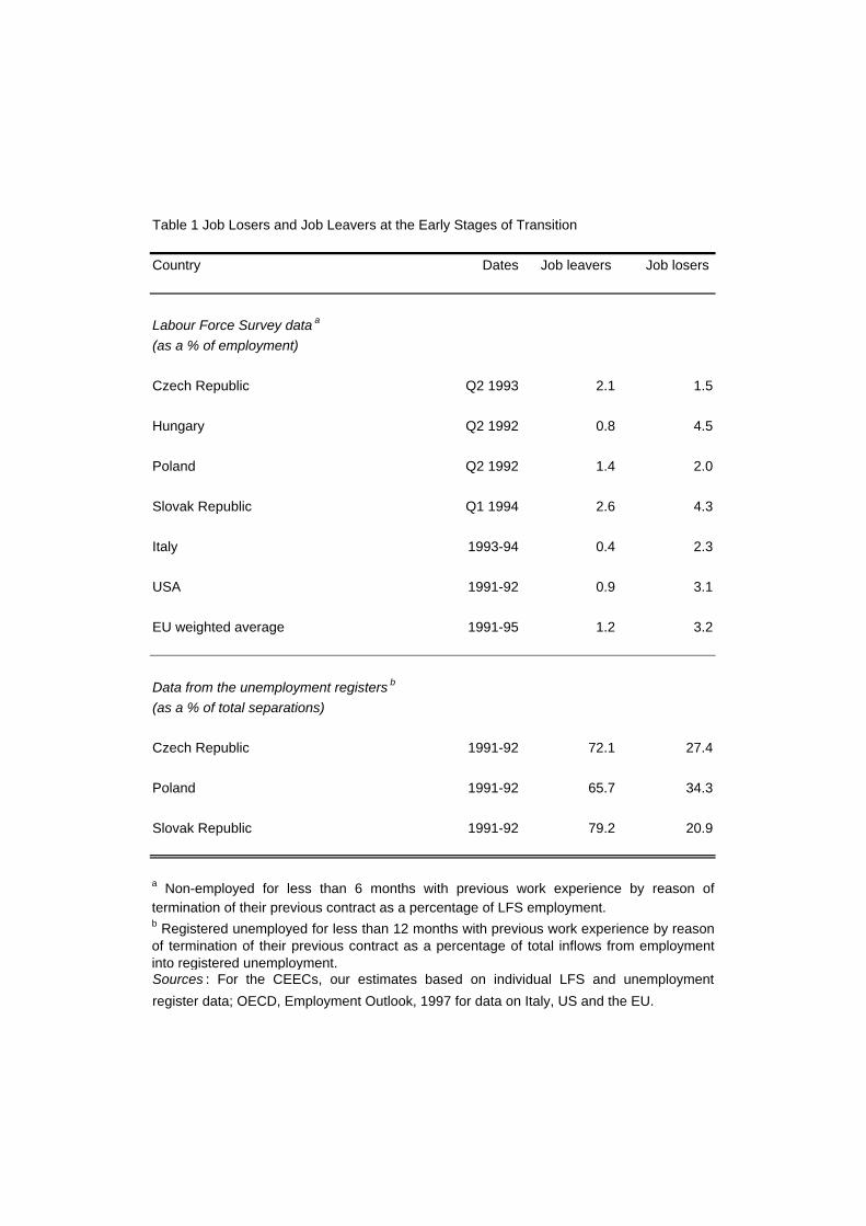
Table 1 Job Losers and Job Leavers at the Early Stages of Transition

Country Dates Job leavers Job losers

Labour Force Survey data a

(as a % of employment)

Czech Republic Q2 1993 2.1 1.5

Hungary Q2 1992 0.8 4.5

Poland Q2 1992 1.4 2.0

Slovak Republic Q1 1994 2.6 4.3

Italy 1993-94 0.4 2.3

USA 1991-92 0.9 3.1

EU weighted average 1991-95 1.2 3.2

Data from the unemployment registers b

(as a % of total separations)

Czech Republic 1991-92 72.1 27.4

Poland 1991-92 65.7 34.3

Slovak Republic 1991-92 79.2 20.9

a Non-employed for less than 6 months with previous work experience by reason oftermination of their previous contract as a percentage of LFS employment. b Registered unemployed for less than 12 months with previous work experience by reasonof termination of their previous contract as a percentage of total inflows from employmentinto registered unemployment. Sources : For the CEECs, our estimates based on individual LFS and unemployment

register data; OECD, Employment Outlook, 1997 for data on Italy, US and the EU.

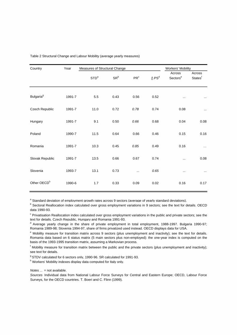
Table 2 Structural Change and Labour Mobility (average yearly measures)

Country Year Measures of Structural Change Workers' Mobility

STDa SRb PRc /\ PSd

Across

Sectorse

Across

Statesf

Bulgariag 1991-7 5.5 0.43 0.56 0.52 ... ...

Czech Republic 1991-7 11.0 0.72 0.78 0.74 0.08 ...

Hungary 1991-7 9.1 0.50 0.66 0.68 0.04 0.08

Poland 1990-7 11.5 0.64 0.66 0.46 0.15 0.16

Romania 1991-7 10.3 0.45 0.85 0.49 0.16 …

Slovak Republic 1991-7 13.5 0.66 0.67 0.74 ... 0.08

Slovenia 1993-7 13.1 0.73 ... 0.65 ... ...

Other OECDh 1990-6 1.7 0.33 0.09 0.02 0.16 0.17

a Standard deviation of employment growth rates across 9 sectors (average of yearly standard deviations).

Notes ... = not available.

h Workers' Mobility indexes display data computed for Italy only.

Sources Individual data from National Labour Force Surveys for Central and Eastern Europe; OECD, Labour ForceSurveys, for the OECD countries. T. Boeri and C. Flinn (1999).

b Sectoral Reallocation index calculated over gross employment variations in 9 sectors; see the text for details. OECDdata 1990-93.c Privatisation Reallocation index calculated over gross employment variations in the public and private sectors; see thetext for details. Czech Republic, Hungary and Romania 1991-93.

e Mobility measure for transition matrix across 9 sectors (plus unemployment and inactivity); see the text for details.Romania data based on 6 status matrix (5 main sectors plus non-employed): the one-year index is computed on thebasis of the 1993-1995 transition matrix, assuming a Markovian process.f Mobility measure for transition matrix between the public and the private sectors (plus unemployment and inactivity);see text for details.

d Average yearly change in the share of private employment in total employment, 1988-1997. Bulgaria 1990-97;Romania 1989-98; Slovenia 1994-97, share of firms privatized used instead. OECD displays data for USA.

g STDV calculated for 6 sectors only, 1990-96. SR calculated for 1991-93.

Figure 1 Labour Market Flows in the Optimal Speed of Transition Literature

Es Ep

U

OLF

allowednot allowed

Notes: ES = employment in state firmsEP = employment in private firmsU = unemploymentOLF = out-of-the labour force

Source : OECD, Short Term Indicators and EBRD Transition Report.

Figure 2

Note : Visegrad Group includes Czech Republic, Hungary, Poland and Slovak Republic. Balkanic Group includes Bulgaria andRomania. USA data refer to the 1929-37 period.

Figure 2b Industrial Production Decline by Transitional Years

50

60

70

80

90

100

110

0 1 2 3 4 5 6 7 8

Years from the start of transition

Bas

e ye

ar =

100 VISEGRAD Group

BALKANIC Group

RUSSIAN FEDERATION

U.S.A.

Figure 2a GDP Decline by Transitional Years

50

60

70

80

90

100

110

0 1 2 3 4 5 6 7 8 9

Years from the start of transition

Bas

e ye

ar =

100

VISEGRAD Group

BALKANIC Group

RUSSIAN FEDERATION

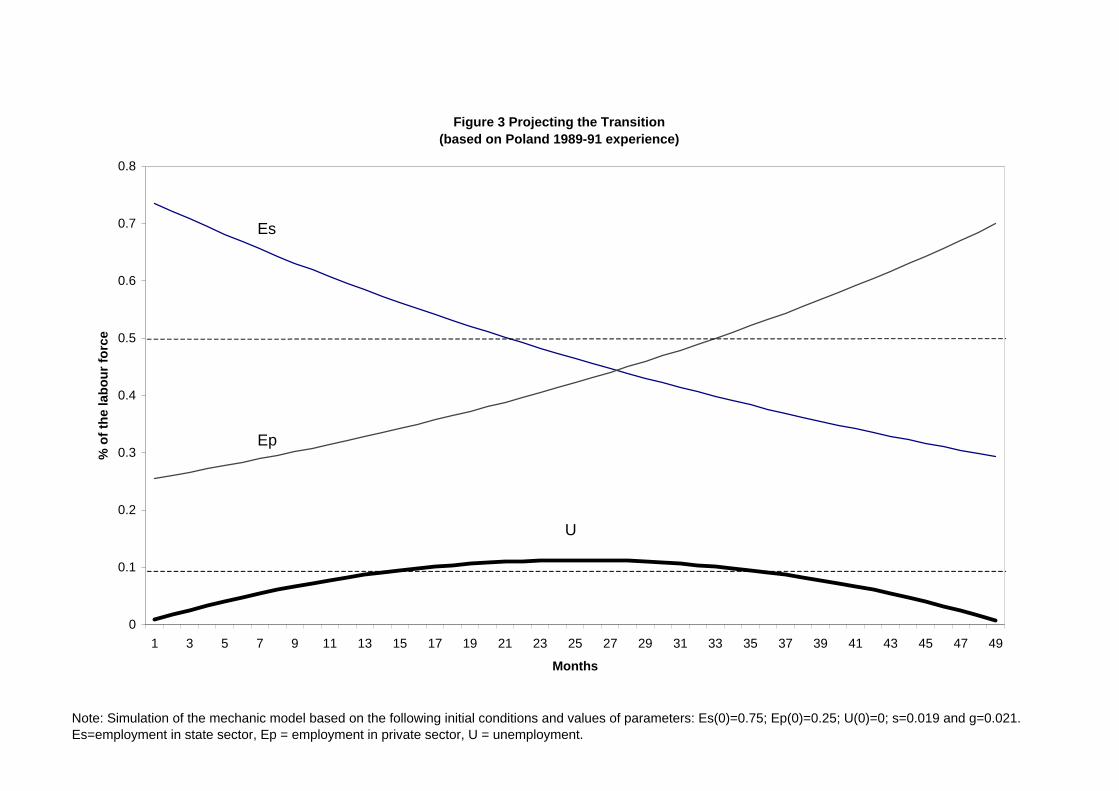
Note: Simulation of the mechanic model based on the following initial conditions and values of parameters: Es(0)=0.75; Ep(0)=0.25; U(0)=0; s=0.019 and g=0.021.Es=employment in state sector, Ep = employment in private sector, U = unemployment.

Figure 3 Projecting the Transition(based on Poland 1989-91 experience)

0

0.1

0.2

0.3

0.4

0.5

0.6

0.7

0.8

1 3 5 7 9 11 13 15 17 19 21 23 25 27 29 31 33 35 37 39 41 43 45 47 49

Months

% o

f th

e la

bo

ur

forc

e

U

Ep

Es

Figure 4 Yearly labour market flows in Poland 1992-1993 (LFS)

Es Ep

U

OLF

8.7

5.9

7.54.3

10.67.8

17.8

24.612

3.9

4.6

4.7

Note: Numbers in the chart denote estimated flows as a percentage of the population of origin.Source: Boeri and Bruno, 1997: matched records across quarterly LFS waves.

Figure 5

Overshooting the decline in Employment Rates

BUL 96

ROM 96 POL 89

POL 96

BUL 89

ROM 89

HUN 96

HUN 89

SLK 96

SLK 89

SLV 96

SLV 89

CZE 96

CZE 89

20

30

40

50

60

70

80

90

0 5000 10000 15000 20000 25000 30000 35000

GDP per capita (USD PPP)

% o

f w

ork

ing

ag

e p

op

ula

tio

n

a Estimated equation: ER = 52,59 + 0,006*GDP pc R2 =0,25Source: OCDE Labour Market Database, World Development Tables, from the OECD National Accounts Report.

Economic growth and employment ratesa

(Middle-income and OECD countries, 1990)

20

30

40

50

60

70

80

90

0 5000 10000 15000 20000 25000 30000 35000

GDP per capita (USD PPP)

% o

f w

ork

ing

ag

e p

op

ula

tio

n

Fig 6a Dis-Employment and decline in participation(1989-1996)

HUNGARY

POLAND

CZECH REPUBLIC

SLOVENIABULGARIA

SLOVAK REPUBLIC

ROMANIA

-0.18

-0.16

-0.14

-0.12

-0.10

-0.08

-0.06

-0.04

-0.02

0.00

-0.18 -0.16 -0.14 -0.12 -0.10 -0.08 -0.06 -0.04 -0.02 0.00

/\ Employment Rate

/\ L

abo

ur

forc

e p

arti

cip

atio

n

Figure 6b Not only females out of the labour market

ROMANIA

SLOVAK REPUBLIC

BULGARIA

SLOVENIA

CZECH REPUBLICPOLAND

HUNGARY

-0.15

-0.10

-0.05

0.00

-0.15 -0.10 -0.05 0.00

/\ male labour force partecipation

/\ fe

mal

e la

bo

ur

forc

e p

arte

cip

atio

n

Annex

Building Blocks of the OST Models

a) The Scale EffectsA key assumption of this literature is that the labour force is fixed to some constant

_

L. Thus,the sum of employment in the public sector (Es), employment in the private sector (Ep) andunemployment (U) can be conveniently normalised to one unit:

Est + Ept + Ut =_

L= 1 1.1

A mechanic model like that outlined in Chapter One is a useful starting point insofar as ithighlights the role played by scale effects in the rise of unemployment. In continuous-time thismechanic model of transition can be rewritten as follows:

Est = Es0−st 1.2

where ”s” denotes, as usual, the pace of closure of state sector jobs, and:

Ept = Ep0egt 1.3

where ”g” is the (instantaneous) rate at which new jobs are created in the private sector.It follows that unemployment evolves according to:

Ut = 1 − Es0e−st − Ep0egt 1.4

The scale effects generate a hump-shaped dynamics of unemployment. In particular, when g= s:

dUdt

= sEst − Ept 1.5

that is, unemployment grows until employment in the private sector is as large asemployment in the state enterprises. After the locus where Es= Ep is reached, unemploymentstarts declining.

b) Endogenous Job Creation

There is no economics in the model sketched above as the dynamics of unemployment isentirely driven by mechanical factors, that is, pure scale effects. In order to assume away scaleeffects and focus only on economics, let us define gross job creation and destruction in terms offlows only, i.e.:

dEstdt

= −st

anddEpt

dt= gt

from which it follows that:dUt

dt= st − gt

Next we endogenise job creation. Along we Aghion and Blanchard (1994) (AB for short), wewill assume that (private) job creation footnote is governed by:

gt = 1 − e1 + ϑ − wt − τt 1.6

where 0 < e < 1 are entry barriers, ϑ is the productivity differential between the public andthe private sectors, whilst w is the (efficiency) wage in the private sector and τ is a (flat) tax perworker in both public and private enterprises earmarked to the financing of unemploymentbenefits footnote . In the AB model, private employers recruit only from the unemploymentranks and pay a premium over the reservation wage of the unemployed, that is, the

unemployment benefit, b. Such a premium can be rationalised either as an incentive device toprevent shirking – e.g., a no-shirking condition, à-la Shapiro-Stiglitz (1984) – or, alternatively, asa way to increase the workers’ loyalty to the firm, that is, a ”gift-exchange” as in Akerlof (1982).Whatever the interpretation for this premium, private wages should be as high as to ensure thatthe value of being employed in the private sector (Vp) exceeds the value of being unemployed,Vu, by some (exogenous) amount, c:

Vpt − Vut = c 1.7

Using then the two asset value conditions for employment in the private sector andunemployment footnote , respectively, one obtains that:

wt = b + cr + gtUt

1.8

where r is the discount rate and the last term within brackets denotes hirings over theunemployment stock, that is, job finding probabilities of the unemployed in this model. Thus, thepremium over unemployment benefits should be larger the higher the wedge between the valueof being employed in the private sector and the value of unemployment, the rate at whichworkers discount future earnings and the probability of being hired once lost a job. Equation(1.8) also shows that unemployment exerts moderating effects on wage setting, which in turn, by(1.6), implies that unemployment boosts job creation in the private sector.

However, there is also a feedback mechanism operating from the fiscal side in AB modelwhich counteracts the effects of unemployment on job creation via wages, namely the financingof unemployment benefits and associated pressures on unit labour costs. Unemployment benefitsare indeed entirely funded out of labour taxation. The budget constraint is therefore given by:

τt1 − Ut = bUt 1.9

hence the tax rate clearing the Government budget is given by:

τt = bUtEst + Ept

1.10

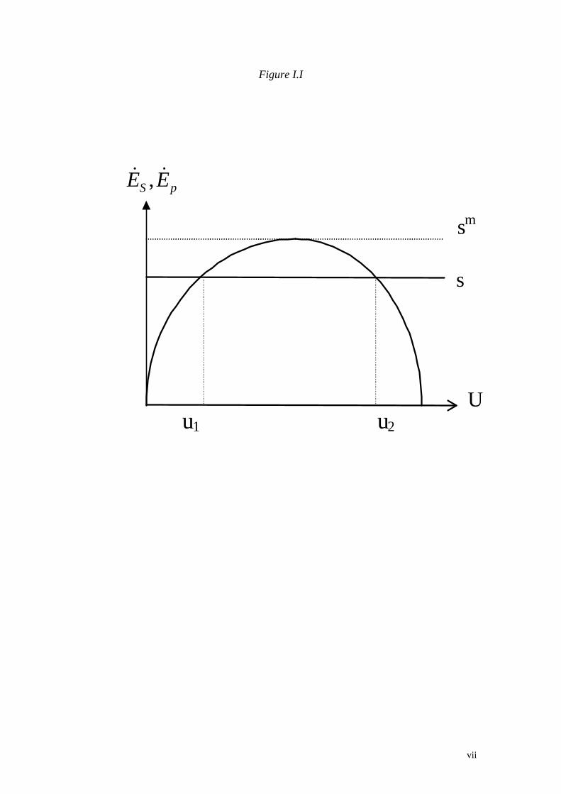
This, together with (1.6), implies that too high unemployment may also negatively affectprivate job creation because of the burden on enterprises associated to paying unemploymentbenefits. This fiscal externality clearly becomes less stringent if deficit financing is allowed for,e.g. , by simply adding a new term (d) on the right-hand-side of (1.9) as in Coricelli (1996).

Due to the presence of the fiscal externality, there is a maximum speed at which public sectorjobs can be destroyed. Above this critical level of s, say s*, transition does not take off as privateemployers are buried under too heavy labour taxation. Moreover, for values of s lower than s*,there can be two equilibria: a low-unemployment equilibrium, like (U1) and ahigh-unemployment equilibrium (U2) as in Figure I.I. When private employers have staticexpectations, from any point to the left of U2 only U1 can be attained while if unemploymentexceeds U2, social security contributions are so high that the private sector grows too slowly toprevent a rise of unemployment or does not take off at all. Thus, the bad equilibrium, U2, isunstable. When private employers are forward-looking (which amounts to adding expectedchanges in the value of private sector jobs on the right-hand-side of (1.6) the economy may settledown at both equilibria. The optimism or pessimism of employers becomes a self-fulfillingprophecy as high job creation reduces labour taxation and vice versa. This holds even whendeficit financing is allowed for.

(insert Figure I.I. about here)

c) Endogenous Job Destruction

The next step is to endogenise job destruction. In these models separations are entirelydemand-driven and dictated by restructuring plans of state enterprises. The latter depend on theextent of employment reductions required to bridge the productivity gap with the private sector.Let f(Es) denote the production function of state enterprises. It is assumed that at the start of

transition everybody is employed in state enterprises footnote and labour productivity thereinequals one unit, that is:

f1 = 1 1.11

State enterprises are overmanned footnote : the restructuring of state enterprises requires thata proportion (1-λ) of the workforce be fired, where λ solves:

fλλ

= 1 + ϑ 1.12

that is, restructuring makes state firms as productive as private firms. State enterprises areassumed to be controlled by insiders who can block privatisation-cum-restructuring plans[Frydman and Rapaczynski, 1994]. All workers of state enterprises are (ex-ante) homogeneousand hence, in the case of restructuring, face the same probability of dismissal, 1-λ. It follows thatrestructuring can start only if:

Vs ≤ λVp + 1 − λVu 1.13

where Vs is the value of being employed in the state sector, Vp the value of being in theprivate sector and Vu the value of being unemployed. In other words, the expected value of thestatus quo should be lower than the expected value of restructuring. As the value ofnon-employment is always lower than the value of employment (either public or private) in thesemodels, when (1.13) is not satisfied, managers should be selective in their dismissal policies andexert a ”divide-and-rule” strategy [Dewatripont and Roland, 1992] in order to convince theirworkforce to accept the restructuring.

As both Vp and Vu decrease with the size of the unemployment pool (the former because ofthe fiscal externality and the latter because job finding probabilities of the unemployed decline) itfollows that there is a critical value of U (say U*) above which restructuring (transition) does nottake-off or is blocked by insiders. Below U*, transition starts and involves increasingunemployment until U* is reached. If the initial shock to state sector employment is too large,however, reductions in unemployment are required to set in motion the restructuring process.This is, in essence, the additional feedback mechanism introduced in the model, coming from theopposition of state sector workers to restructuring.

d) The Balanced Path footnote

Normalising rVs to equal one unit, and taking into account (1.7) and the definitions for thevalue of being employed in the private and unemployed, we can rewrite (1.13) as follows:

1 ≤ λw + 1 − λw − cr 1.14

and when the above condition holds has an equality (when we are along the balanced path):

w = 1 + 1 − λcr 1.15

which states that there should be a wedge (increasing in the probability ofdismissal footnote ) between the wage paid in the private and in the state sector in order toinduce workers to accept restructuring.

We can finally solve for the equilibrium level of unemployment satisfying (1.14). First, weequate (1.14) to the wage setting equation (8). Next we substitute in this expression the jobcreation equation (1.6) (leaving aside, for simplicity, the fiscal externality effect) and solve for Uobtaining:

U∗ = c1 − eθ − 1 − λ cr1 − b − λ cr

1.16

The equilibrium speed of transition, s*, will be such as to maintain unemployment at U*. Inother words, s should be as large as to equate unemployment inflows (s times the proportion ofworkers to be laid-off) to outflows when U=U*. Equating then private job creation (1.6) tos1 − λ, when (14) is satisfied, one obtains:

s∗λ = 1 − eϑ − 1 − λcr 1.17

which shows that the equilibrium speed is increasing in the productivity gap and decreasingin entry barriers (exogenous obstacles to gross job creation) and the efficiency wage premium.

Notice that by (1.15), equilibrium unemployment is increasing in unemployment benefits.However, too low benefits may prevent the start of transition especially when the costs ofunemployment benefits is only partly internalised by firms (e.g., benefits are paid out of generalfiscal revenues footnote , private firms are de facto exempted from social security contributions –e.g., due to weak tax enforcement – or Governments receive a gift like foreign loans atconcessional terms to pay benefits). When the Government budget constraint (1.9) is not binding,higher benefits increase the asset value of unemployment and hence reduce the opposition ofinsiders to restructuring. We have indeed that:

∂Vu

∂b= 1

1 + r1 − cr1 − e

U + c 1.18

which shows that, on the one hand, higher benefits increase the instantaneous value ofunemployment, but, on the other hand, reduce the job-finding probability of those without a job.This second effect tends to dominate the effect of benefits on the instantaneous utility whenbenefits are entirely funded via payroll taxation. In the latter case we find indeed that:

∂Vu

∂b= 1

1 + rU + c1 − UU + c1 − U − cr1 − e 1.19

which becomes negative for large U.Overall, insofar as benefits can be financed without increasing payroll taxes, high

unemployment benefits reduce the resistance of insiders to restructuring and permit the take-offof transition. This is the standard result of the OST literature. However, when higher benefitsimply heavier taxation of labour in the private sector, the negative effects of benefits on jobgeneration in the private sector tend to dominate, as the transition proceeds, those on the(instantaneous) welfare of the unemployed. From this point onward it is better to reduceunemployment benefits to ease restructuring. In order words, the optimal sequence is ”high”benefits followed by ”low” benefits.

vii

Figure I.I

u1 u2

pS EE && ,

U

s

sm