OPTIMAL QUADRATIC NITSCHE EXTENDED FINITE ELEMENT … · Optimal Quadratic Nitsche Extended Finite Element Method for Interface Problem of Di usion Equation 3 In this paper, we study

Journal of Computational Mathematics

Vol.xx, No.x, 200x, 1–25.

http://www.global-sci.org/jcm

doi:10.4208/jcm.1703-m2015-0340

OPTIMAL QUADRATIC NITSCHE EXTENDED FINITEELEMENT METHOD FOR INTERFACE PROBLEM OF

DIFFUSION EQUATION*

Fei Wang

School of Mathematics and Statistics, Xi’an Jiaotong University, Xi’an, Shaanxi 710049, China.

Department of Mathematics, Pennsylvania State University, University Park, PA 16802, USA.

Email: [email protected]

Shuo Zhang

LSEC, ICMSEC, NCMIS, Academy of Mathematics and System Sciences, Chinese Academy of

Sciences, Beijing 100190, Peoples Republic of China.

Email: [email protected]

Abstract

In this paper, we study Nitsche extended finite element method (XFEM) for the inter-

face problem of a two dimensional diffusion equation. Specifically, we study the quadratic

XFEM scheme on some shape-regular family of grids and prove the optimal convergence

rate of the scheme with respect to the mesh size. Main efforts are devoted onto classifying

the cases of intersection between the elements and the interface and prove a weighted trace

inequality for the extended finite element functions needed, and the general framework of

analysing XFEM can be implemented then.

Mathematics subject classification: 65N30, 65N12, 65N15.

Key words: Interface problems, Extended finite element methods, Error estimates, Nitsche’s

scheme, Quadratic element.

1. Introduction

Many problems in physics, engineering, and other fields contain a certain level of coupling

between different physical systems, such as the coupling between fluid and structure in fiuid-

structure interaction problems, and the coupling among different flows in multi-phase flows

problems. An interface where the coupling takes place is generally encountered in such kind of

problems, and, consequently, the numerical discretization of the interface problem is important

in applied sciences and mathematics. In this paper, we take the diffusion equation

−∇ · (α(x)∇u) = f, (1.1)

as a model problem, and study its interface problem. Namely, the underlying domain is assumed

to be divided to two subdomains by an interface, such that α is smooth on each subdomain,

but not smooth on the whole domain. The model problem is a fundamental one in numerical

analysis, and very incomplete literature review can be found in, e.g., [4,5,14,30,31] and below.

Different from problem with smooth coefficient, the existence of an interface for diffusion

equation can invalidate the global smoothness of the solution of the system, and the accuracy

of the standard finite element method is limited when used for such problems. As the loss of

* Received July 22, 2015 / Revised version received November 14, 2016 / Accepted March 23, 2017 /

Published online xxxxxx xx, 20xx /

2 F. WANG AND S. ZHANG

accuracy occurs near the interface, where the solution is no longer smooth, the obstacle can be

circumvented by implementing a body-fitted (or interface-resolved) grid. In this approach, the

“bad part” of the solution that may not be well approximated is restricted in a narrow region

surrounding the interface. We refer the reader to [30] for an asymptotic optimal error estimate

on body-fitted grid:

‖u− uI‖0,Ω + h|u− uI |1,Ω ≤ C| log h|1/2h2|u|2,Ω1∪Ω2 ,

where uI is the linear element interpolation for u ∈ H1(Ω)∩H2(Ω1∪Ω2). We use |w|m,Ω1∪Ω2 or

‖w‖m,Ω1∪Ω2 to denote |w|m,Ω1 + |w|m,Ω2 or ‖w‖m,Ω1 + ‖w‖m,Ω2, respectively, for w ∈ Hm(Ω1 ∪Ω2) := v ∈ L2(Ω) : v|Ωi

∈ Hm(Ωi), i = 1, 2. A sharper estimate without the logarithmic

factor was given in Bramble and King [4] (1996):

‖u− uI‖0,Ω + h|u− uI |1,Ω 6 Ch2|u|2,Ω1∪Ω2 . (1.2)

We also refer to [5, 14, 31] for related discussions. Unfortunately, it is usually a nontrivial

and time-consuming task to construct good interface-fitted meshes for problems involving ge-

ometrically complicated interfaces. Another idea is to add some basis functions which can be

non-smooth around the interface so that the nonsmooth part of the solution can be accurately

captured. By enriching the finite element space with local basis functions that can resolve the

interface, numerous modified methods based only on simple Cartesian grids are proposed. For

finite element methods, we refer to the work of [6, 16] for elliptic problems with discontinuous

coefficients, where finite element basis functions are. modified at the coefficients discontinuity.

Extra work around the interface can also be recognised implemented in the finite difference

setting; we refer to, e.g., [24] for the immersed boundary method, to [13, 15] for the immersed

interface method, to [19] for the ghost fluid method and etc..

The extended finite element method (XFEM) falls into the category of the second approach.

The XFEM extends the classical finite element method by enriching the solution space locally

around the interface with nonsmooth functions, and it is realized through the partition of unity

concept. Developed by Belytschko and his collaborators ([3,21]), the XFEM is originally used for

modelling crack growth, and has now been used widely in crack propagation ([3,8,21,22]), fluid-

structure interaction (FSI) ([9, 28]), multi-phase flows ([10]), and other multi-physics problems

that involve interfaces. This approach provides accurate approximation for the problems with

jumps, singularities, and other locally nonsmooth features within elements. We refer to [7] and

the reference therein for a historical account for XFEM.

The Nitsche-XFEM scheme presented in [11] is a special kind of XFEM which can also be

regarded as the coupling of the continuous finite element method and discontinuous Galerkin

(DG) method. In [11], Nitsche’s formulation of an elliptic interface problem was introduced, and

then the extended finite element space is constructed by enriching the standard finite element

space with functions that are completely discontinuous across the interface; stabilisation terms

are then needed for the stability of the scheme. The Nitsche-XFEM uses essentially piecewise

polynomials and flexibility can be expected respectively in designing schemes of various orders

and in implementing. The optimality of the Nitsche-XFEM scheme for interface problem is

proved when the XFE space consists of linear continuous piecewise basis functions and extended

basis functions constructed by partition of unity in [11]. Technically, a crucial fact is that the

gradient of a linear polynomial is constant. This fact does not hold for polynomials of higher

degrees, and so far as we know, the analysis of the high-order Nitsche-XFEM is still absent.

Optimal Quadratic Nitsche Extended FEM for Interface Problem 3

In this paper, we study the quadratic Nitsche-XFEM for the interface problem, where the

XFE space is constructed based on the continuous piecewise quadratic element space. We

prove the consistency and the stability of the scheme, and finally the optimal convergence.

Technically, the most significant step is to construct a trace inequality (3.2) (Lemma 3.2) for

piecewise quadratic polynomials. As the shape of interface intersecting an element may take

various forms and the gradient of the finite element function is no longer a constant, a detailed

analysis has to be carried out with respect to each of the cases. We clarify and classify all the

cases, and construct the inequality for a wide class of interfaces. It thus follows that the second

order scheme is proven to be optimally convergent. This can subsequently be extended to be

applied for moving interface problems.

We notice there have been works devoted to the DG-type method for the interface problems.

A new immersed finite element method with Nitsche formulation on interface was introduced

in [18] for solving parabolic interface problem on structured Cartesian meshes, and the optimal

convergence rate in an energy norm was proved. In [20], an unfitted symmetric interior penalty

discontinuous Galerkin method for 2D elliptic interface problems was studied, and optimal

convergence for arbitrary polynomial degree was given in an energy norm and in the L2 norm.

Again, the intersection between the interface and the cells is a focus of the discussion therein.

However, Assumption 3.3 in [20] is strong, and it may not be clear to the readers for which cases

the assumption could be true. An additional constraint is also required, whereas the author

only considered some special cases where it is assumed that the interface only intersects with

the boundary of each element at two points that lie on different edges. An unfitted hp-interface

penalty finite element method for elliptic interface problems was studied in [29], where penalty

term for the flux (normal derivative) was added in the bilinear form of the discretization scheme.

This modification makes the stability provable by only using one side local trace and inverse

inequalities, namely on the larger sub-element, and the inequalities on smaller sub-element do

not have to be considered. This extra flux penalty term, however, does not seem necessary

for second order problems and it makes the bilinear form for discrete problems inconsistent

with the continuous problem. In this paper, we utilize a bilinear form without this high-order

stabilization term and prove the stability and the convergence of the resulting scheme.

The remaining of the paper is organized as follows. In next section, we introduce some

preliminaries, including an interface problem of the diffusion equation, extended finite element

method, Nitsche’s formulation of the interface problem and its XFEM discretization. In Section

3, we study the stability for Nitsche-XFEM scheme when a quadratic element space is used and

prove the optimal convergence rate of the scheme. The key step is a trace inequality, for which

we present a detailed proof. Numerical experiments are reported in Section 4 to verify the

theoretical analysis. Finally, some concluding remarks are given at the last section.

2. Preliminaries

In this section, we introduce the elliptic interface problem. Then, we introduce the extended

finite element space and its best approximation property. Finally, we reformulate the interface

problem according to Nitsche’s scheme, and use XFE for its discretization.

2.1. An interface problem

Let Ω ⊂ R2 be a convex domain and Ω = Ω1 ∪ Ω2 with Γ = ∂Ω1 ∩ ∂Ω2 being a smooth

closed curve and Γ ∩ ∂Ω = ∅ (see Fig 2.1). We consider the following interface problem


−∇ · (α(x)∇u) = f, in Ω,

[α(x)∇u] = 0, on Γ,

[u] = ~0, on Γ,

u = 0, on ∂Ω,

(2.1)

where the jump coefficient

α(x) =

α1, if x ∈ Ω1,

α2, if x ∈ Ω2.

Here, [u] and [α(x)∇u] are the jumps of u and its flux across interface Γ, respectively. The

jump [·] is defined in (2.6) and (2.7).

Ω2

Ω1

Γ

Fig. 2.1. Domain for an interface problem.

Given a bounded domain,D ⊂ R2, and a positive integer,m,Hm(D) is the standard Sobolev

space with the corresponding usual norm and semi-norm, which are denoted respectively by

‖ · ‖m,D and | · |m,D. The norm of Lebesgue space L2(D) is denoted by ‖ · ‖D.

The variational formulation of the above problem is: Find u ∈ H10 (Ω) s.t.

a(u, v) =

∫

Ω

fv dx, ∀v ∈ H10 (Ω),

where

a(u, v) =

∫

Ω

α(x)∇u · ∇v dx.

When f ∈ L2(Ω), the solution u of (2.1) is piecewise smooth; namely, u ∈ V := H10 (Ω)∩H2(Ω1∪

Ω2) and ‖u‖H1(Ω) + ‖u‖H2(Ω1) + ‖u‖H2(Ω2) 6 C‖f‖0,Ω; globally, V ⊂ H3/2−ǫ(Ω) for any ǫ > 0,

but V 6⊂ H2(Ω); we refer to, e.g., [2,5,12,17,26,27] for details and related discussion. The loss

of regularity makes the approximation of the standard finite element space non-optimal.

2.2. An extended finite element with respect to the interface

To save the approximation accuracy, following [10], we construct the eXtended finite element

space (XFES). In this section and throughout the paper, we assume Ω is a polygonal domain


and let T 0 be a coarse triangulation of Ω that covers Ω exactly. By dividing each triangle into

four triangles uniformly and repeating this refine procedure successively, we get a family of

triangulations T(T 0) = T jJj=0 of Ω starting from T 0. This sequence of triangulations form

a shape-regular family; any edge in Th ∈ T(T 0) can find a parallel edge in T 0. Through this

paper, we assume the grid Th is chosen from this family. Without ambiguity, we use Th for the

grid under discussion, with h denoting for the mesh size. For a mesh Th, Let hK = diam(K)

and h = maxhK : K ∈ Th. Let T Γh = K ∈ Th, K ∩ Γ 6= ∅ be the set of all triangles

that intersect with Γ. Let eK = K ∩ Γ, Ki = K ∩ Ωi and ~ni = ~n|∂Kibe the unit outward

normal vector on ∂Ki with i = 1, 2. For an edge e, its tangential direction is assigned to be

its orientation. In this context, we do not distinguish a direction and its opposite direction.

Evidently, two parallel edges have the same orientation.

Remark 2.1. As the interface Γ has finite number of turning points, given an orientation,

the number of points in Γ where the tangential line is along the given orientation is finite.

Therefore, since the number of the orientations of the edges in Th ∈ T(T 0) is the same as the

number of the orientations of the edges in T 0, for any given interface Γ, the number of possible

tangent points of Γ with mesh Th is uniformly bounded.

Given a mesh Th, let Vh be the continuous piecewise p-th degree polynomial space on the

mesh for p > 1, and let Ih be the usual interpolation associated with Vh. Let χi be the

characteristic function on subdomain Ωi, i.e., χi = 1 on Ωi, and χi = 0 on Ω\Ωi. Define the

XFE space by

V Xh = V 1

h + V 2h ,

with

V ih := χi · Vh :=

χi(x)vh(x), ∀vh ∈ Vh

.

It is clear that the extended finite element functions are simply constructed by dividing the

finite element functions by the interface. Actually, the XFE space can be regarded as a standard

FE space plus an enrichment space, see the following lemma.

Lemma 2.1 ([10]) V Xh = Vh + V Γ

h , where V Γh consists of functions whose support are located

in the elements intersected by the interface, and that are discontinuous across the interface.

Denote by Epi a continuous extension operator from Hp(Ωi) to H

p(Ω), i = 1, 2, p > 1. For

u ∈ Hp+1(Ω1 ∪ Ω2), define

Πhu = χ1IhEp+11 (u|Ω1) + χ2IhE

p+12 (u|Ω2), (2.2)

where Ih is the usual nodal interpolation operator on Vh. The following lemma shows the best

approximation property of the interpolation Πhu defined above.

Lemma 2.2. There exists a constant C depending on Ω and Γ only, such that it holds for

u ∈ Hp+1(Ω1 ∪ Ω2) that

‖u−Πhu‖0,Ω ≤ Chp+1(‖u‖p+1,Ω1 + ‖u‖p+1,Ω2

), (2.3)

|u −Πhu|1,Ωi≤ Chp‖u‖p+1,Ωi

, i = 1, 2, (2.4)(∑

K∈Th

|u−Πhu|22,Ωi∩K

)1/2

≤ Chp−1(‖u‖p+1,Ω1 + ‖u‖p+1,Ω2

), i = 1, 2. (2.5)


Proof. By the definition of the interpolation, we have

u−Πhu = (χ1 + χ2)u− (χ1Ihu1 + χ2Ihu2) = χ1(u1 − Ihu1) + χ2(u2 − Ihu2),

and

∇(u−Πhu)|Ωi= ∇(ui − Ihui)|Ωi

, i = 1, 2.

Therefore, we obtain

‖u−Πhu‖20,Ω ≤ ‖u1 − Ihu1‖20,Ω + ‖u2 − Ihu2‖20,Ω≤ C(h2p+2‖u1‖2p+1,Ω + h2p+2‖u2‖2p+1,Ω)

≤ Ch2p+2(‖u‖2p+1,Ω1+ ‖u‖2p+1,Ω2

).

Similarly,

|u −Πhu|21,Ωi= |(ui − Ihui)|21,Ωi

≤ Ch2p‖ui‖2p+1,Ω ≤ Ch2p‖u‖2p+1,Ωi, i = 1, 2,

(∑

K∈Th

|u−Πhu|22,Ωi∩K

)1/2

≤ Chp−1(‖u‖p+1,Ω1 + ‖u‖p+1,Ω2), i = 1, 2.

This finishes the proof.

2.3. Nitsche’s formulation for the interface problems

Associated with the interface and the triangulation Th, we introduce the following notation.

For a scalar-valued function v, let vi = v|∂Ki, and similarly, for a vector-valued function ~q, we

denote ~qi = ~q|∂Ki. Define the weighted average · and the jump [·] on eK ⊂ Γ by

v = β1v1 + β2v2, [v] = v1~n1 + v2~n2, (2.6)

~q = β1~q1 + β2~q2, [~q] = ~q1 · ~n1 + ~q2 · ~n2, (2.7)

where βi =|Ki||K| . Without ambiguity, we briefly use |D| for the measure of a geometric domain

D. For example, for an edge eK , |eK | denotes its length.Next, we rewrite interface problem (2.1) following Nitsche’s scheme. Let u ∈ V be the

solution of (2.1) and v ∈ V , then direct calculation leads to

∫

Ω

fv dx =

∫

Ω

α(x)∇u · ∇v dx−∫

Γ

α(x)∇u · [v] ds−∫

Γ

[u] · α(x)∇v ds+∫

Γ

µ[u] · [v] ds,

for any µ ∈ R. Nitsche’s formulation of the interface problem is to find u ∈ V such that

B(u, v) =

∫

Ω

fv dx, ∀v ∈ V, (2.8)

where the bilinear form B(·, ·) is defined for u, v ∈ H2(Ω1 ∪ Ω2) by

B(u, v) :=

∫

Ω

α(x)∇u ·∇v dx−∫

Γ

α(x)∇u · [v] ds−∫

Γ

[u] · α(x)∇v ds+∫

Γ

µ[u] · [v] ds. (2.9)


2.4. Nitsche XFEM for interface problems

The extended finite element problem of Nitsche’s formulation for interface problem (2.1) is

to find uh ∈ V Xh , such that

B(uh, vh) =

∫

Ω

fvh dx, ∀vh ∈ V Xh , (2.10)

where

B(u, v) =

∫

Ω

α(x)∇u · ∇v dx−∑

K∈T Γh

∫

eK

α(x)∇u · [v] ds

−∑

K∈T Γh

∫

eK

[u] · α(x)∇v ds +∑

K∈T Γh

∫

eK

ηeKh−1K [u] · [v] ds. (2.11)

Here, we choose µ|eK = ηeKh−1K , with ηeK being a constant number.

Note for the cases that eK = Γ∩K is not connected, that is, eK = e1K ∪e2K is separated into

two disconnected curves e1K and e2K , that K is also divided into 3 parts, K = K(1)1 ∪K(2)

1 ∪K2

with K2 = K ∩Ω2 and K(1)1 ∪K(2)

1 = K ∩Ω1. Correspondingly, in the bilinear form (2.11), we

also separate them as two terms, which means∫eKv ds =

∫e1K

v ds +∫e2K

v ds, and the weights

of the average · defined on eK are modified to be the weights of the average defined on eiK as

β(i)1 =

|K(i)1 |

|K(i)1 |+ |K2|

and β(i)2 =

|K2||K(i)

1 |+ |K2|, with i = 1, 2.

The following lemma shows that the exact solution also satisfies the Nitsche XFEM formu-

lation (2.10).

Lemma 2.3 ([11]) Let u be the solution of (2.1), then

B(u, vh) =

∫

Ω

f vh dx ∀ vh ∈ V Xh . (2.12)

To consider the boundedness and stability of the bilinear form, we define the broken DG

norms. Denote V (h) = V + V Xh , and define on V (h) the norms by

‖v‖2w = |v|21,Ω1∪Ω2+∑

K∈T Γh

h−1K ‖[v]‖20,eK and ‖v‖2∗ = ‖v‖2w +

∑

K∈T Γh

hK‖∇v‖20,eK . (2.13)

We have the following lemma for the boundedness and stability of the bilinear form.

Lemma 2.4 ([1, 11] Boundedness and Stability) If η0 = infeK ηeK > 0 is large enough,

then,

B(u, v) ≤ Cb‖u‖∗ ‖v‖∗ ∀u, v ∈ V (h), (2.14)

B(v, v) ≥ Cs‖v‖2w ∀ v ∈ V Xh , (2.15)

where Cb and Cs are positive constants depending on the jump coefficient α, the angle condition,

the polynomial degree, and a bound on the edge-dependent penalty parameter η.

Note that there is a gap as two norms used for the boundedness and stability above are different.

The gap is fulfilled when V Xh is the extended finite element space generated based on the

standard linear element space (linear extended finite element space), and an optimal convergence

rate is obtained.


2.4.1. The convergence of the scheme

The XFE space provides optimal approximation to V in the norm ‖ ·‖∗. To show this, we begin

with the trace inequality below.

Lemma 2.5 ([10, 11]) For any v ∈ H1(K), we have the following trace inequality.

‖v‖20,eK ≤ C(h−1K ‖v‖20,K + hK |v|21,K

). (2.16)

Here, C is a constant independent of v, K and eK .

Then we have the following lemma for the approximation property of the XFE interpolation

to a function u ∈ H1(Ω) ∩Hp+1(Ω ∪ Ω2).

Lemma 2.6. It holds for u ∈ H1(Ω) ∩Hp+1(Ω ∪ Ω2) that

‖u−Πhu‖∗ ≤ Chp(|u|p+1,Ω1 + |u|p+1,Ω2

). (2.17)

Proof. By the definition of norm ‖ · ‖∗, we have

‖u−Πhu‖2∗=∑

i=1,2

|u−Πhu|21,Ωi+∑

K∈T Γh

hK‖∇(u−Πhu)‖20,eK +∑

K∈T Γh

h−1K ‖[u−Πhu]‖20,eK .

Then, we use the trace inequality (2.16) to get

hK‖∇(u−Πhu)‖20,eK ≤ 2∑

i=1,2

hK‖∇(ui − Ihui)‖20,eK ,

≤C∑

i=1,2

(|ui − Ihui|21,K + h2K |ui − Ihui|22,K

)≤ Ch2p

(|u1|2p+1,K + |u2|2p+1,K

)

and

h−1K ‖[u−Πhu]‖20,eK ≤ 2

∑

i=1,2

h−1K ‖ui − Ihui‖20,eK

≤C∑

i=1,2

(h−2K ‖ui − Ihui‖20,K + |ui − Ihui|21,K

)≤ Ch2p

(|u1|2p+1,K + |u2|2p+1,K

).

Combining these with the results in Lemma 2.2, we finish the proof.

Lemma 2.7 ([11]) Let V Xh be the linear extended finite element space, and let u and uh be the

solution of (2.8) and (2.10), respectively. Assume u ∈ H10 (Ω) ∩ H2(Ω1 ∪ Ω2). Then it holds

that

‖u− uh‖∗ 6 Ch|u|2,Ω1∪Ω2 , (2.18)

where C is a positive constant that depends on interface Γ, the angle condition, and a bound on

the edge-dependent penalty parameter ηeK .

In the next section, we consider the accuracy when a second degree XFES is used.


3. Optimality of the Quadratic Nitsche-XFEM

In this section, we consider the accuracy of the Nitsche-XFEM where V Xh is constructed

based on the continuous quadratic element space (quadratic extended finite element space).

The main result of this paper is the following theorem.

Theorem 3.1. Let V Xh be the quadratic extended finite element space on Th, and let u and uh

be the solutions of (2.1) and (2.10), respectively, and assume u ∈ H10 ∩H3(Ω1 ∪Ω2). Then, it

holds that

‖u− uh‖∗ ≤ Ch2(|u|3,Ω1 + |u|3,Ω2

), (3.1)

where C is a positive constant that depends on interface Γ, the angle condition, and a bound on

the edge-dependent penalty parameter η.

We postpone the proof of this theorem to Section 3.1 after some technical lemmas. Lemma

3.2 is a key result; we postpone its proof to Section 3.2 due to its length and detailed nature.

3.1. Stability of the scheme and its convergence

Property 3.2. Let t be the arc length parameter, and ~r(t) = (f(t), g(t)) with t ∈ [0, T ] be a

parametric description of the closed curve Γ that satisfies the following conditions:

1. ~r(t) ∈ (C2[0, T ])2, and |~r ′(t)| 6= 0 for t ∈ [0, T ];

2. the number of turning points of Γ, namely the points on a curve where the curve changes

from being concave to convex or vice versa, is finite;

3. there exists an integer N and a constant M , such that for any t0 ∈ [0, T ], there exists an

integer n ≤ N , such that ~r(k)(t0) ·~ν(t0) = 0 for k ≤ n− 1, and 0 < |~r (n)(t0) ·~ν(t0)| < M ,

where ~ν(t0) is the normal vector of interface Γ at point (f(t0), g(t0)).

Remark 3.1. Geometrically, ~r (k)(t0) · ~ν(t0) = 0 for k = 1, · · · , n− 1, but ~r (n)(t0) · ~ν(t0) 6= 0

means that the interface curve ~r(t) has point-contact of order n with its tangent line ~r ′(t0)

at point ~r(t0) ([25]). The order of point-contact is independent of the parametrization and

unchanged under rotations, reflexions, or translations. In practice, most smooth curves we deal

with satisfy Property 3.2. A turning point is referred to a point ~r(t) for some t ∈ [0, T ] such

that ~r (i)(t) · ~ν(t) = 0 for i = 2, · · · , k − 1 and ~r (k)(t0) · ~ν(t0) 6= 0 for some odd number k.

Lemma 3.1. Let Γ satisfy Property 3.2, and T be a family of quasi-uniform triangulations.

Given δ ∈ (0, 1), there exists an h0 > 0, such that when the mesh size h ≤ h0, it holds for any

K ∈ T Γh ⊂ Th ∈ T that there is at most one turning point in K and there exists a constant

number δ > 0 such that

|~r ′(t1) · ~r ′(t2)| > δ for any ~r(t1), ~r(t2) ∈ eK .

Proof. As there are a fixed finite number of turning points, they are separable. So when h

is small enough, the turning points are separated by the mesh. Since ~r(t) ∈ (C2[0, T ])2, for any

t1 and t2 satisfying ~r(ti) ∈ eK , it holds that

|~r ′(t1)− ~r ′(t2)| ≤ |~r ′′(t)||t1 − t2| ≤ ChK , with t1 ≤ t ≤ t2.

Therefore, |~r ′(t1) · ~r ′(t2)| > δ. This finishes the proof.


Lemma 3.2. Let Γ satisfy Property 3.2. Then, there exist two constants C and h0, depending

only on Γ, such that on any quasi-uniform Th with h 6 h0, we have

∑

K∈T Γh

hK‖∇v‖20,eK ≤ C‖v‖2w, ∀v ∈ V Xh . (3.2)

This lemma is a key step in the analysis. When V Xh is the XFES based on linear element space,

∇v is piecewise constant, and the inequality is proved by comparing the area of K and the

length of e. When V Xh is of second degree, however, the case is more complicated. We postpone

its proof in Section 3.2.

By Lemma 3.2, we have the lemma below.

Lemma 3.3. The norms ‖v‖w and ‖v‖2∗ are equivalent on V Xh when h is sufficiently small.

That is, there exist two constants C and h0, depending only on Γ, such that on any quasi-

uniform Th with h 6 h0, we have

‖v‖2w ≤ ‖v‖2∗ ≤ C‖v‖2w, ∀v ∈ V Xh .

Now, we give the stability of the bilinear form B(u, v).

Lemma 3.4 (Stability) If η0 = infe ηe > 0 is large enough and h is sufficiently small, the

bilinear form B(·, ·) is coercive:

B(v, v) ≥ Cs‖v‖2∗ ∀ v ∈ V Xh , (3.3)

where Cs is a positive constant depending on the jump coefficient α, the angle condition, the

polynomial degree, and a bound on the edge-dependent penalty parameter η.

Proof. We know that ‖v‖w and ‖v‖2∗ are equivalent on V Xh by Lemma 3.3; then, by (2.15),

the coercivity of B(v, v) holds true on V Xh with ‖v‖∗ as well, so that (3.3) hold true.

Proof of Theorem 3.1 Let Πhu be the interpolant of u in the V Xh . Recall the boundedness

and stability of the bilinear form B. We have

Cs‖Πhu− uh‖2∗ ≤ B(Πhu− uh,Πhu− uh)

= B(Πhu− u,Πhu− uh) +B(u − uh,Πhu− uh)

≤ Cb‖Πhu− u‖∗ ‖Πhu− uh‖∗

Note that by consistency (Lemma 2.3), B(u − uh,Πhu− uh) = 0. Then,

‖Πhu− uh‖∗ ≤ Cb/Cs‖Πhu− u‖∗ ≤ Ch2(|u|3,Ω1 + |u|3,Ω2

). (3.4)

Write the error as

u− uh = (u−Πhu) + (Πhu− uh),

and use the triangle inequality

‖u− uh‖∗ = ‖u−Πhu‖∗ + ‖Πhu− uh‖∗≤ (1 + Cb/Cs)‖Πhu− u‖∗ ≤ Ch2(|u|3,Ω1 + |u|3,Ω2).



3.2. Proof of Lemma 3.2

In this section, we prove the Lemma 3.2. To this end, we only need to prove that there is

a constant C independent of how the interface intersect with elements, and only depends on

interface Γ such that

hK‖∇v‖20,eK ≤ C(‖∇v‖20,K1+ ‖∇v‖20,K2

)

for each K ∈ T Γh , where we recall eK = K ∩ Γ and sub-elements Ki = K ∩ Ωi with i = 1, 2.

The main idea of proof for Lemma 3.2 is based on the inequality in the following lemma.

Lemma 3.5. Let eK = Γ∩K and Ki = K∩Ωi for some K ∈ T Γh . Let Ki ⊂ Ki be any (curved)

triangle with eK as one of its edges. Let K0i and K∗

i be two triangles such that K0i ⊆ Ki ⊆ K∗

i .

Denote

Ci = supv∈P1(K∗

i )

‖v‖20,∞,K∗

i

‖v‖20,∞,K0

i

, (3.5)

Di =|Ki||K0

i |. (3.6)

Then, we have

hK‖∇v‖20,eK ≤2C∑

i=1,2

CiDihK |eK ||Ki|2|K|−2|Ki|−1‖∇vi‖20,Ki,

where C is a constant only dependent of the shape-regularity of the grid.

Proof. Note that if Ki is a (curved) triangle, Ki can be chosen as Ki. We choose two

triangles K0i and K∗

i such that K0i ⊆ Ki ⊆ K∗

i . Then for any v ∈ P1(K) we have

1

|eK |

∫

eK

v2 ds ≤ ‖v‖20,∞,eK ≤ ‖v‖20,∞,K∗

i≤ Ci‖v‖20,∞,K0

i.

Furthermore, by scaling argument, we obtain

‖v‖20,∞,K0i= ‖v‖2

0,∞,K≤ C‖v‖2

0,2,K

=C

|K0i |

∫

K0i

v2 dx ≤ C

|K0i |

∫

Ki

v2 dx ≤ CDi

|Ki|

∫

Ki

v2 dx,

where C is constant number only depending on the reference element K. Therefore, we get∫

eK

v2 ds ≤ CCiDi|eK ||Ki|

∫

Ki

v2 dx. (3.7)

Then, we obtain

hK‖∇v‖20,eK ≤2hK

(β21‖∇v1‖20,eK + β2

2‖∇v2‖20,eK)

≤2C∑

i=1,2

CiDihK |eK ||Ki|2|K|−2|Ki|−1‖∇vi‖20,Ki.


In the following argument, we construct special Ki,K0i ,K

∗i for each Ki, and prove

CiDihK |eK ||Ki|2|K|−2|Ki|−1 ≤ C, (3.8)

case by case, which completes the proof of Lemma 3.2. The technical arguments are listed in

the following subsections.


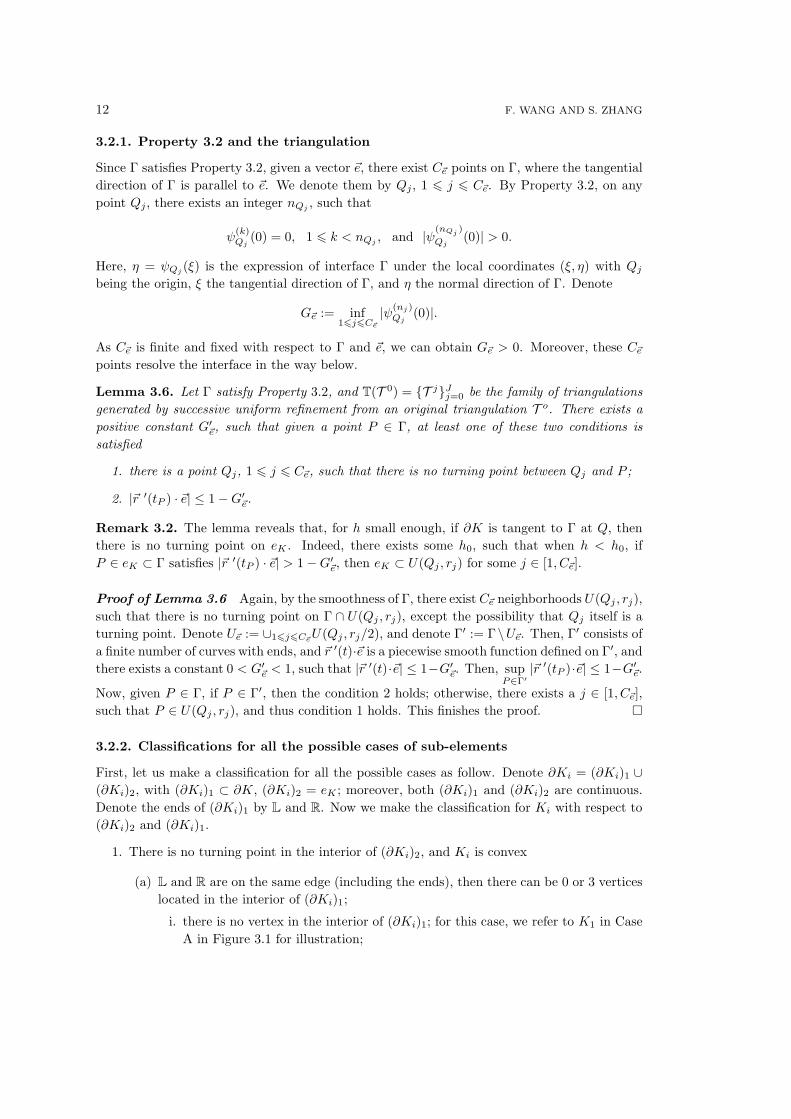
3.2.1. Property 3.2 and the triangulation

Since Γ satisfies Property 3.2, given a vector ~e, there exist C~e points on Γ, where the tangential

direction of Γ is parallel to ~e. We denote them by Qj, 1 6 j 6 C~e. By Property 3.2, on any

point Qj, there exists an integer nQj, such that

ψ(k)Qj

(0) = 0, 1 6 k < nQj, and |ψ(nQj

)

Qj(0)| > 0.

Here, η = ψQj(ξ) is the expression of interface Γ under the local coordinates (ξ, η) with Qj

being the origin, ξ the tangential direction of Γ, and η the normal direction of Γ. Denote

G~e := inf16j6C~e

|ψ(nj)Qj

(0)|.

As C~e is finite and fixed with respect to Γ and ~e, we can obtain G~e > 0. Moreover, these C~e

points resolve the interface in the way below.

Lemma 3.6. Let Γ satisfy Property 3.2, and T(T 0) = T jJj=0 be the family of triangulations

generated by successive uniform refinement from an original triangulation T o. There exists a

positive constant G′~e, such that given a point P ∈ Γ, at least one of these two conditions is

satisfied

1. there is a point Qj, 1 6 j 6 C~e, such that there is no turning point between Qj and P ;

2. |~r ′(tP ) · ~e| ≤ 1−G′~e.

Remark 3.2. The lemma reveals that, for h small enough, if ∂K is tangent to Γ at Q, then

there is no turning point on eK . Indeed, there exists some h0, such that when h < h0, if

P ∈ eK ⊂ Γ satisfies |~r ′(tP ) · ~e| > 1−G′~e, then eK ⊂ U(Qj , rj) for some j ∈ [1, C~e].

Proof of Lemma 3.6 Again, by the smoothness of Γ, there exist C~e neighborhoods U(Qj , rj),

such that there is no turning point on Γ ∩ U(Qj , rj), except the possibility that Qj itself is a

turning point. Denote U~e := ∪16j6C~eU(Qj , rj/2), and denote Γ′ := Γ\U~e. Then, Γ

′ consists of

a finite number of curves with ends, and ~r ′(t)·~e is a piecewise smooth function defined on Γ′, and

there exists a constant 0 < G′~e < 1, such that |~r ′(t)·~e| ≤ 1−G′

~e. Then, supP∈Γ′

|~r ′(tP )·~e| ≤ 1−G′~e.

Now, given P ∈ Γ, if P ∈ Γ′, then the condition 2 holds; otherwise, there exists a j ∈ [1, C~e],

such that P ∈ U(Qj , rj), and thus condition 1 holds. This finishes the proof.

3.2.2. Classifications for all the possible cases of sub-elements

First, let us make a classification for all the possible cases as follow. Denote ∂Ki = (∂Ki)1 ∪(∂Ki)2, with (∂Ki)1 ⊂ ∂K, (∂Ki)2 = eK ; moreover, both (∂Ki)1 and (∂Ki)2 are continuous.

Denote the ends of (∂Ki)1 by L and R. Now we make the classification for Ki with respect to

(∂Ki)2 and (∂Ki)1.

1. There is no turning point in the interior of (∂Ki)2, and Ki is convex

(a) L and R are on the same edge (including the ends), then there can be 0 or 3 vertices

located in the interior of (∂Ki)1;

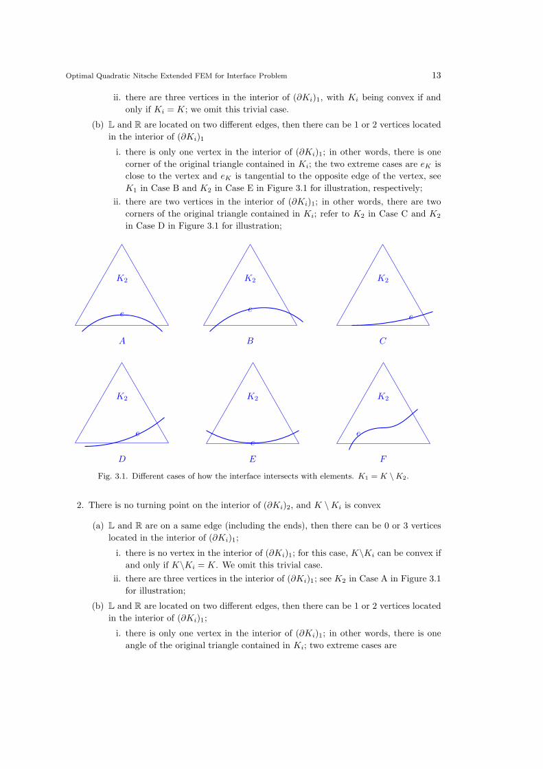
i. there is no vertex in the interior of (∂Ki)1; for this case, we refer to K1 in Case

A in Figure 3.1 for illustration;


ii. there are three vertices in the interior of (∂Ki)1, with Ki being convex if and

only if Ki = K; we omit this trivial case.

(b) L and R are located on two different edges, then there can be 1 or 2 vertices located

in the interior of (∂Ki)1

i. there is only one vertex in the interior of (∂Ki)1; in other words, there is one

corner of the original triangle contained in Ki; the two extreme cases are eK is

close to the vertex and eK is tangential to the opposite edge of the vertex, see

K1 in Case B and K2 in Case E in Figure 3.1 for illustration, respectively;

ii. there are two vertices in the interior of (∂Ki)1; in other words, there are two

corners of the original triangle contained in Ki; refer to K2 in Case C and K2

in Case D in Figure 3.1 for illustration;

e

A

K2

e

B

K2

e

C

K2

e

D

K2

e

E

K2

e

F

K2

Fig. 3.1. Different cases of how the interface intersects with elements. K1 = K \K2.

2. There is no turning point on the interior of (∂Ki)2, and K \Ki is convex

(a) L and R are on a same edge (including the ends), then there can be 0 or 3 vertices

located in the interior of (∂Ki)1;

i. there is no vertex in the interior of (∂Ki)1; for this case, K\Ki can be convex if

and only if K\Ki = K. We omit this trivial case.

ii. there are three vertices in the interior of (∂Ki)1; see K2 in Case A in Figure 3.1

for illustration;

(b) L and R are located on two different edges, then there can be 1 or 2 vertices located

in the interior of (∂Ki)1;

i. there is only one vertex in the interior of (∂Ki)1; in other words, there is one

angle of the original triangle contained in Ki; two extreme cases are


A. eK is tangential to one of the edges where the ends of (∂Ki)1 lie; K1 in Case

C in Figure 3.1 for illustration.

B. eK is away from the edges where the ends of (∂Ki)1 lie; refer to K1 in Case

D in Figure 3.1 for illustration;

ii. there are two vertices in the interior of (∂Ki)1; in other words, there are two

angles of the original triangle contained in Ki; two extreme cases are

A. eK is tangential to the edge of the two vertices; see K1 in Case E in Figure

3.1 for illustration;

B. eK is away from the edge of the two vertices, ; refer to K2 in Case B in

Figure 3.1 for illustration;

3. There is one turning point on the interior of (∂Ki)2

By Lemma 3.6, we know that a tangent point and a turning point can be avoided to

be present at same element if mesh size is small enough, so obviously, there are two

possibilities, namely Ki is a curved triangle and Ki is a curved quadrilateral, respectively;

see K1 and K2 in Case F in Fig 3.1 for an illustration.

By Lemma 3.1, there is no other possibility. We obtain for anyK ∈ T Γh such that eK = Γ∩K

is continuous and any subelement Ki = K ∩ Ωi, there exist triangles Ki, and K0i ⊂ Ki ⊂ K∗

i ,

such that (3.8) holds when Ki is convex, K \Ki is convex, or there is a turning point on eK ,

by Lemmas 3.7, 3.8 and 3.9, respectively. Then, the proof of Lemma 3.2 is finished by Lemma

3.5.

C

F

A BD EO

G

K2

∗

∗

∗∗

∗

∗∗

Case A

A

B

C

D

E

K2

F

∗∗∗

∗

∗

Case B

e∗ ∗∗

∗ ∗C A

B

D E

K2

Case C

Fig. 3.2. Cases that eK does not contain a turning point.

3.2.3. Proof of Lemma 3.2 for convex sub-element Ki

Lemma 3.7. Fix K ∈ T Γh and let eK = Γ ∩ K with a convex sub-element Ki = K ∩ Ωi.

Then, there exists a (curved) triangle Ki ⊂ Ki with eK as one of its edges, and there exist two

triangles, K0i and K∗

i , such that K0i ⊂ Ki ⊂ K∗

i and (3.8) holds true with Ci and Di defined

in (3.5) and (3.6).

Proof. Now, we verify the three possible cases one by one.


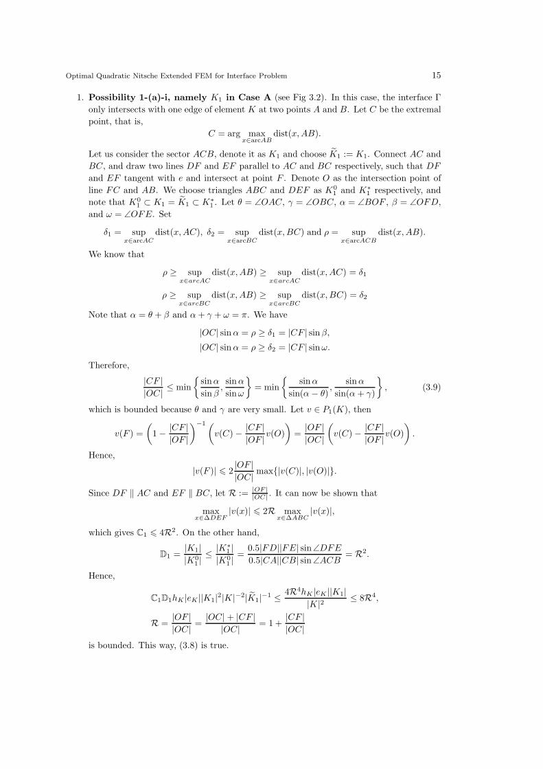
1. Possibility 1-(a)-i, namely K1 in Case A (see Fig 3.2). In this case, the interface Γ

only intersects with one edge of element K at two points A and B. Let C be the extremal

point, that is,

C = arg maxx∈arcAB

dist(x,AB).

Let us consider the sector ACB, denote it as K1 and choose K1 := K1. Connect AC and

BC, and draw two lines DF and EF parallel to AC and BC respectively, such that DF

and EF tangent with e and intersect at point F . Denote O as the intersection point of

line FC and AB. We choose triangles ABC and DEF as K01 and K∗

1 respectively, and

note that K01 ⊂ K1 = K1 ⊂ K∗

1 . Let θ = ∠OAC, γ = ∠OBC, α = ∠BOF , β = ∠OFD,

and ω = ∠OFE. Set

δ1 = supx∈arcAC

dist(x,AC), δ2 = supx∈arcBC

dist(x,BC) and ρ = supx∈arcACB

dist(x,AB).

We know that

ρ ≥ supx∈arcAC

dist(x,AB) ≥ supx∈arcAC

dist(x,AC) = δ1

ρ ≥ supx∈arcBC

dist(x,AB) ≥ supx∈arcBC

dist(x,BC) = δ2

Note that α = θ + β and α+ γ + ω = π. We have

|OC| sinα = ρ ≥ δ1 = |CF | sinβ,|OC| sinα = ρ ≥ δ2 = |CF | sinω.

Therefore,

|CF ||OC| ≤ min

sinα

sinβ,sinα

sinω

= min

sinα

sin(α − θ),

sinα

sin(α+ γ)

, (3.9)

which is bounded because θ and γ are very small. Let v ∈ P1(K), then

v(F ) =

(1− |CF |

|OF |

)−1(v(C)− |CF |

|OF |v(O))

=|OF ||OC|

(v(C)− |CF |

|OF |v(O)).

Hence,

|v(F )| 6 2|OF ||OC| max|v(C)|, |v(O)|.

Since DF ‖ AC and EF ‖ BC, let R := |OF ||OC| . It can now be shown that

maxx∈∆DEF

|v(x)| 6 2R maxx∈∆ABC

|v(x)|,

which gives C1 6 4R2. On the other hand,

D1 =|K1||K0

1 |≤ |K∗

1 ||K0

1 |=

0.5|FD||FE| sin∠DFE0.5|CA||CB| sin∠ACB = R2.

Hence,

C1D1hK |eK ||K1|2|K|−2|K1|−1 ≤ 4R4hK |eK ||K1||K|2 ≤ 8R4,

R =|OF ||OC| =

|OC| + |CF ||OC| = 1+

|CF ||OC|

is bounded. This way, (3.8) is true.


e∗ ∗

∗

∗

∗∗∗

∗∗ ∗ ∗H C

A

B

D

E

F

G

K2

O

QM

S

T

Case D

O

e1 e2∗

∗∗∗ ∗

A

C

D

E GB

F

K2

Case E

Fig. 3.3. Cases that eK does not contain a turning point.

2. Possibility 1-(b)-i , namely K1 in Case B (Fig 3.2) and K2 in Case E (Fig 3.3).

Let us prove (3.8) for K1 in Case B here and same argument applies to K2 in Case E.

In this case, we choose K1 = K1. Connect B and C to get triangle ABC denoted by

K01 . Then, draw a line DE parallel to line BC and tangential to e. Let K∗

1 denote the

triangle ADE, then K01 ⊂ K1 = K1 ⊂ K∗

1 . If R = ADAB = AE

AC ≤ 2, we know that

C1 ≤ 4R2 and D1 ≤ R2 are bounded, which finishes the proof of (3.8). If R > 2, that

is, |DB| > |AB|, then 2|K1| > |K1|. So we only need to apply the same argument of

K1 in Case A for K1 = K1\K01 to prove that, there exist K0

1 ⊂ K1 ⊂ K∗1 , such that

C1 = supv∈P1(K∗

1 )

‖v‖20,∞,K∗

1

‖v‖2

0,∞,K01

and D1 = |K1|

|K01 |

are bounded. Then, by Lemma 3.5, we have

1

|e|

∫

e

v2 ds ≤ CC1D11

|K1|

∫

K1

v2 dx ≤ 2CC1D11

|K1|

∫

K1

v2 dx,

which completes the proof of (3.8).

3. Possibility 1-(b)-ii, namely K2 in Case C (see Fig 3.2) and K2 in Case D (see Fig

3.3).

Here, let us take K2 in Case D to show the proof. Connect the non-adjacent vertices

to get diagonals CG and BH , and they intersect at point O. Denote ∠BOG, ∠OCB

and ∠CBO by α, β, and γ, respectively. Let K2 ⊂ K2 be the (curved) triangle with e

as one of its edge and make choice so that the area of K2 is larger. Namely, we choose

(curved) triangle BCG as K2 if β ≥ γ, or choose (curved) triangle BCH as K2 otherwise.

Without loss of generality, we assume that β ≥ γ. Then we know that β < α ≤ 2β due to

α = β+γ. If β ≤ π/4, we have sinαsin β ≤ sin 2β

sin β = 2 cosβ < 2. If β > π/4, then sinβ > 1/√2,

and sinαsin β <

√2. So, for both cases,

|K2||K2|

≤12 |BH ||CG| sinα12 |BC||CG| sin β

<2|BH ||BC| . (3.10)


From the previous argument, we can prove there exists K02 ⊂ K2 ⊂ K∗

2 , such that

C2 = supv∈P1(K∗

2 )

‖v‖20,∞,K∗

2

‖v‖20,∞,K0

2

, D2 =|K2||K0

2 |

are bounded and (3.7) hold true. Therefore, we get

C2D2hK |eK ||K2|2|K|−2|K2|−1 < 2C2D2hK |eK ||K2||K|−2|BH ||BC|−1 ≤ C.

Summing all above finishes the proof.

3.2.4. Proof of Lemma 3.2 for sub-element Ki, with K \Ki being convex

Lemma 3.8. Let K ∈ T Γh and Ki = K ∩Ωi be a sub-element with its complement K\Ki being

convex. There is a (curved) triangle Ki ⊂ Ki with eK being one of its edges and two triangles,

K0i and K∗

i with K0i ⊂ Ki ⊂ K∗

i such that (3.8) holds true with Ci and Di defined in (3.5) and

(3.6).

Proof. Now we verify the possible cases one by one.

1. Possibility 2-(b)-i-A, namely K1 in Case C ( see Fig 3.2). Interface Γ is tangent

with AC ⊂ ∂K at point C, and intersects ∂K at another point B. The curved triangle

ABC is K1, and let K1 = K1. Connect points B and C, and draw a line, BD, tangent

to e at point B, and intersecting AC at point D. Let BE be perpendicular to AC and

intersect with AC at point E. Denote the triangles ABC and DAB by K∗1 and K0

1 ,

respectively. Then we have K01 ⊂ K1 = K1 ⊂ K∗

1 . Similarly, let R = |AC||AD| , we have

C1 ≤ 4R2. Furthermore, vD =|CD||AC| vA +

(1− |CD|

|AC|

)vC . Then, we have

vA =

(1− |CD|

|AC|

)−1(vD − |CD|

|AC| vB)

= R(vD − |CD|

|AC| vB).

So, C1 ≤ 4R2 and in addition,

D1 =|K1||K0

1 |≤ |K∗

1 ||K0

1 |=

0.5|AC||BE|0.5|AD||BE| = R.

In local coordinates, set point C ((f(t0), g(t0)) as the origin, and CA as ξ-coordinate.

Then, Γ can be expressed as η = ψ(ξ) in these local coordinates with ψ(0) = ψ′(0) = 0.

By definition 3.2, we know that there exists a number, n ≤ N , such that ψ(n)(0) 6= 0

([25]), so we have

ψ(ξ) =1

n!ψ(n)(0)ξn +

1

(n+ 1)!ψ(n+1)(ξ)ξn+1.

Then, there is a small number ǫ depending on Γ and h such that

1− ǫ

n!ψ(n)(0)ξn ≤ ψ(ξ) ≤ 1 + ǫ

n!ψ(n)(0)ξn,

1− ǫ

(n− 1)!ψ(n)(0)ξn−1 ≤ ψ′(ξ) ≤ 1 + ǫ

(n− 1)!ψ(n)(0)ξn−1


where

ǫ = sup0≤ξ≤l

ξ

n+ 1

∣∣∣∣∣ψ(n+1)(ξ)

ψ(n)(0)

∣∣∣∣∣ .

Here, l = |CE|. As the number of possible tangential points is uniformly finite with

respect to Γ and T0, for all these points tiPi=1, ~r(n)(ti) ·~ν(ti) has a uniform lower bound,

meaning |ψ(n)(0)| has a uniform lower bound, C0. Therefore, ǫ→ 0 as h→ 0.

Elementary calculus leads to

1− ǫ

(1 + ǫ)nl ≤ ψ(l)

ψ′(l)≤ 1 + ǫ

(1− ǫ)nl,

so (1− 1 + ǫ

(1− ǫ)n

)l ≤ l − ψ(l)

ψ′(l)≤(1− 1− ǫ

(1 + ǫ)n

)l.

Hence, we have

R =

(1− |CD|

|AC|

)−1

≤(1− |CD|

|CE|

)−1

≤ (1 + ǫ)n

1− ǫ,

which is bounded, because n is uniformly bounded for non-degenerate smooth curves and

ǫ→ 0 when h→ 0. Therefore,

C1D1hK |eK ||K1||K|−2 ≤ 4R3h−2K |K1|

is bounded. The proof of (3.8) is finished for this case.

2. Possibility 2-(a)-ii, namely K1 in Case D (see Fig 3.3). Here, curved triangle ABC

is K1 and choose K1 = K1. Without loss of generality, we assume that |AB| ≤ |AC|.We draw a line CE tangent to e at point C and intersecting AB at point E. Denote the

triangles ABC and ACE by K∗1 and K0

1 , respectively. Then, we have K01 ⊂ K1 = K1 ⊂

K∗1 . As in Case C, we have C1 ≤ 4R2 and D1 ≤ R, with R = |AB|

|AE| . If R is bounded, then

the proof is complete. If not, we see that |AC||AE| does not have a lower bound. Then by

Lemma 3.6, there is a pointM on Γ near C, and its the tangential direction of Γ is parallel

to AH . Draw a line BD tangent with e at point B, and intersect with AC at point D.

Draw a tangential line of Γ from M , which intersects with the extension of GA at Q.

Connect BM which intersects AH at S. Note that S is not necessarily between A and H .

Extend BD to intersect MQ at T . The inner triangle K01 is ABD, the outer triangle K∗

1

is ABS. Note |AS|/|AD| = |QM |/|QT | and |∆ABS|/|∆ABD| = |∆QBM |/|∆QBT |.Then, we use the conclusion of Case C to finish the proof of (3.8) for this case.

3. Possibility 2-(b)-ii-A, namely K1 in Case E (see Fig 3.3). Next, let us consider the

case that interface Γ intersects with ∂K at 3 points, denoted by C, O and D. Note that

O is a tangent point, which separates the eK = Γ ∩K into two parts denoted by e1 and

e2. Let us consider the inequality for K1. The tangent point O separates the K1 as two

curved triangles, K(1)1 (curved triangle AOC) and K

(2)1 (curved triangle BOD). Again, set

O as the origin and OB as the ξ-coordinate. Then, locally the interface eK is expressed

as

ψ(ξ) =1

n!ψ(n)(0)ξn +

1

(n+ 1)!ψ(n+1)(ξ)ξn+1,


and there is a small number ǫ depending on Γ and h such that

1− ǫ

n!ψ(n)(0)ξn ≤ ψ(ξ) ≤ 1 + ǫ

n!ψ(n)(0)ξn. (3.11)

Note that n should be an even number due to the shape of e in this case. Without loss of

generality, we assume that |AO| ≥ |BO|, by the relation (3.11) and direct calculation, we

know that there exist two constants C1 and C2, only depending on ǫ such that |BD| ≤C1|AC| and |K(2)

1 | ≤ C2|K(1)1 |. So |K1| = |K(2)

1 |+ |K(1)1 | ≤ (1 + C2)|K(1)

1 |.Choose K1 = K1 and draw a line CE that is tangent to e1 at point C. Let us denote

the triangle AEC by K01 . Connect points C and D, and denote the quadrilateral ABDC

by K∗1 . From previous argument, we know that R = |AO|

|AE| ≤ (1+ǫ)n1−ǫ and

|K(1)1 |

|K01 |

≤ R.

Therefore, we have|AB||AE| ≤

2|AO||AE| ≤ 2(1 + ǫ)n

1− ǫ.

We know that

vB =|AB||AE|

(vE − |BE|

|AB|vA),

vF =|AF ||AC|

(vC − |FC|

|AF |vA),

vF =|BF ||BD|

(vD − |FD|

|BF |vB).

By some manipulations, we get

vD =|BD||AF ||AC||BF | vC − |BD||FC|

|AC||BF | vA +|FD||BF |vB .

Because we assume that each element K is shape regular, there exists a constant C3 only

depending on the shape-regularity of the grid such that

|AF | ≤ C3|BF |.

By simple calculation, we have

|vB | ≤2(1 + ǫ)n

1− ǫ(|vE |+ |vA|),

|vD| ≤(C1C3 +

2(1 + ǫ)n

1− ǫ

)(|vA|+ |vC |+ |vE |),

which implies that C1 ≤ 9(C1C3 +

2(1+ǫ)n1−ǫ

)2. Furthermore, we have

D1 =|K1||K0

1 |=

|K1||K(1)1 |

|K(1)1 ||K0

1 |≤ (1 + C2)

(1 + ǫ)n

1− ǫ.

We see that both C1 and D1 are bounded, so (3.8) holds true for this case.

Note, if point O does not touch AB, but the distance to AB is very small, then we

draw a tangent line of eK on point O, which intersects with AF and BF at A′ and B′,

respectively. Let K1 denote K1\ABB′A′. Then, we make similar argument for K1 to

prove (3.8).


4. Possibility 2-(a)-ii and 2-(b)-ii-B, namely K2 in Case A and B (see Fig 3.2).

K2 in Case A. Let us connect points GA and GB and choose the curved triangle GAB

as K2. Then, from the previous argument, we prove that there exists K02 ⊂ K2 ⊂ K∗

2 ,

and C2 and D2 are two bounded constants such that (3.7) holds true. Furthermore, it is

easy to see that|K2||K2|

<2hK|eK | .

Therefore, we get

C2D2hK |eK ||K2|2|K|−2|K2|−1 < 2C2D2h2K |K2||K|−2 < C.

K2 in Case B. Let us connect points F and C and choose the curved triangle FCB as

K2. Then, from the previous argument, we again prove that there exists K02 ⊂ K2 ⊂ K∗

2 ,

and C2 and D2 are two bounded constants such that (3.7) holds true. Furthermore, by

the same argument for (3.10), we get

|K2|+ ǫ

|K2|+ ǫ≤ 2hK

|eK | ,

where ǫ = |CDFE| − |K2| ≤ C0h3K . So, if |DF | > h2K , equivalently, ǫ ≤ C0|K2|, then

|K2||K2|

≤ C0hK|eK | .

Therefore, we get

C2D2hK |eK ||K2|2|K|−2|K2|−1 < 2C2D2h2K |K2||K|−2 < C.

If |DF | ≤ h2K , then it is reduced to K1 in Case E.

Summing all above finishes the proof.

3.2.5. Proof of Lemma 3.2 when eK contains a turning point

Lemma 3.9. Let eK = Γ ∩K contain a turning point. Then, we can find a (curved) triangle

Ki ⊂ Ki with eK as one of its edges, and two triangles, K0i and K∗

i , such that K0i ⊂ Ki ⊂ K∗

i

and (3.8) holds true with Ci and Di defined in (3.5) and (3.6).

Proof. Obviously, there are two possibilities, namely Ki is a curved triangle or Ki is a

curved quadrilateral, respectively; see K1 and K2 in Case F in Fig 3.4 for an illustration. We

analyze the two cases below.

1. K1 in Case F (see Fig 3.4). Here, K1 is the curved triangle ABC. We choose K1 = K1.

Then, draw a line CD going through point C, tangent to eK and intersect AB at D to

get triangle ADC denoted by K01 , and then draw a line EF parallel to CD, and tangent

with eK to get triangle AEF denoted by K∗1 . We still have K0

1 ⊂ K1 = K1 ⊂ K∗1 . Let

R = AEAD = AF

AC , then C1 ≤ 4R2 and D1 ≤ R2. We know that if R is bounded, the proof

is finished. Otherwise, let H be the turning point on eK , separating eK as e1 and e2,


∗

∗

∗

∗∗∗∗

A

D

EB

F C

K1

K2

G

H

I

Case F

Fig. 3.4. Case that eK contains a turning point.

which do not contain turning point. Let HI be perpendicular to AC and intersect with

AC at point I, and K1 is divided into K(1)1 and K

(2)1 by HI.

Applying the similar argument of K1 in Case B for K(1)1 , and similar argument of K2 in

Case B for K(2)1 , we prove that there exist K

(i)01 ⊂ K

(i)1 ⊂ K

(i)∗1 , such that C

(i)1 and D

(i)1

are bounded and

∫

ei

v2 ds ≤ CC(i)1 D

(i)1

|ei||K(i)

1 |

∫

K(i)1

v2 dx, i = 1, 2.

Without loss of generality, we assume that |e2|

|K(2)1 |

≤ |e1|

|K(1)1 |

. Then there exists a constant C1

such that δ1 ≤ C1δ2, where δ1 = supx∈arcCH dist(x,AC) and δ2 = supx∈arcHB dist(x,AC).

Let l1 = |CI| and l2 = |IA|. If l1 ≤ l2, then |K(1)1 | ≤ C1|K(2)

1 |, and we choose K(2)01

as K01 , and the convex hull of K1 as K∗

1 to apply the same argument of K1 in Case D

to prove (3.8). Otherwise, l2 = lα1 for some α > 1. Then, C1 ≤ l1+l2l2

= 1 + l1−α1 and

D1 ≤ D(2)1

l1+l2l2

= D(2)1 (1 + l1−α

1 ).

Because |e2|

|K(2)1 |

≤ |e1|

|K(1)1 |

, we have

hKβ22‖v‖20,eK ≤ ChK

|K1|2|K|2

∑

i=1,2

|ei||K(i)

1 |

∫

K(i)2

v2 dx

≤ 2ChK(|K(1)

1 |+ |K(2)1 |)2

|K|2|e1|

|K(1)1 |

∫

K1

v2 dx

= 2ChK|K(1)

1 |2 + 2|K(1)1 ||K(2)

1 |+ |K(2)1 |2

|K|2|e1|

|K(1)1 |

∫

K1

v2 dx.

It is easy to see thathk|e1||K

(1)1 |

|K|2 andhk|e1||K

(2)1 |

|K|2 are bounded, so we only need to consider


whether the termhk|e1||K

(2)1 |2

|K|2|K(1)1 |

is bounded. We know that if δ1 ≥ l22δ22

h3K

,

hk|e1||K(2)1 |2

|K|2|K(1)1 |

≤ Cl22δ

22

h3Kδ1≤ C.

Otherwise,

C1D1hK |eK ||K1|2|K|−2|K1|−1 ≤ Cl2−2α1 |K1||K|−1 ≤ C

l21δ1l1l22h

2K

≤ Cl31δ

22

h5K≤ C.

This completes the proof for this case.

2. K2 = K\K1 in Case F (see Fig 3.4). Here, K2 is a curved quadrilateral. Let us connect

points C and G and choose the curved triangle CBG as K2. Then, by the previous

argument, it is proved that there exists K01 ⊂ K1 = K1 ⊂ K∗

1 and two bounded constants

C2 and D2 such that (3.7) holds true. Furthermore, by the same argument for (3.10), we

get|K2|+ ǫ

|K2|+ ǫ≤ 2hK

|eK | ,

where ǫ ≤ C0h3K . Then, if |BG| > h2K , namely ǫ ≤ C0|K2|, we have

|K2||K2|

≤ C02hK|eK | .

Therefore, we get

C2D2hK |eK ||K2|2|K|−2|K2|−1 ≤ 2C2D2h2K |K2||K|−2 ≤ C.

If |DF | ≤ h2K , then it is reduced to K1 in the Case F, which have been proved before.

Summing up all above finishes the proof.

4. Numerical Example

In this section, we present numerical verification of the convergence rate of the quadratic

Nitsche-XFEM for interface problem.

Denote the domain Ω := (0, 1)2 and let the interface Γ be the zero level set of the function

φ(x) = (x1 − 0.5)2 + (x2 − 0.5)2 − 1/8. We consider the model problem (2.1). Specifically, the

right hand side is chosen so that the exact solution is

u(x) =

1/α1 exp(x1x2), x ∈ Ω1 = x ∈ Ω, φ(x) < 0,1/α2 sin(πx1) sin(πx2), x ∈ Ω2 = x ∈ Ω, φ(x) > 0.

We apply the quadratic Nitsche-XFEM with the penalty parameter ηeK = 10.

Figure 4.1 shows the numerical results of the quadratic Nitsche-XFEM method for solving

the interface problem. The blue cross (×) and red star (*) denote the errors in H1 norm and

L2 norm, respectively. The black and blue lines are the reference lines of slopes -2 and -3. It

can be observed that the convergence orders match well with the theoretical predictions.


100

101

102

log10

(1/h)

10-6

10-5

10-4

10-3

10-2

10-1

log

10(e

rror)

Error in H1 norm

Error in L2 norm

h2

h3

Fig. 4.1. Numerical errors of the quadratic Nitsche-XFEM method.

5. Concluding Remarks

In this paper, we study the quadratic Nitsche-XFE scheme for the elliptic interface problem,

and prove its optimal convergence rate. A key step in the proof of the stability is to show a

trace inequality, for which we study in detail the cases how the interface may intersect the edges

of the grid, and finally verify the result for each of them. The convergence result then follows

under the general framework.

As the interface problem of the diffusion equation is encountered more and more frequently

from both theoretical research and practical application, and the accuracy and the flexibility

would be among issues with most interests, it is natural to generalize the construction and

analysis in the present paper to the schemes of higher degrees and of other DG types. These

will be discussed in the future.

Acknowledgements. The first author is partially supported by the U.S. Department of

Energy, Office of Science, Office of Advanced Scientific Computing Research as part of the

Collaboratory on Mathematics for Mesoscopic Modeling of Materials under Award Number

DE-SC-0009249, and the Key Program of National Natural Science Foundation of China with

Grant No. 91430215. The second author is supported by State Key Laboratory of Scientific

and Engineering Computing (LSEC), National Center for Mathematics and Interdisciplinary

Sciences of Chinese Academy of Sciences (NCMIS), and National Natural Science Foundation of

China with Grant No. 11471026; he is thankful to the Center for Computational Mathematics

and Applications, the Pennsylvania State University, where he worked on this manuscript as

a visiting scholar. The authors are grateful to Professor Jinchao Xu, Dr. Yuanming Xiao and

Dr. Maximilian Metti for their valuable suggestions and discussions, to Professor Haijun Wu

for his valuable help on preparing the numerical example, and to the anonymous referee for the

valuable comments and suggestion which lead to improvements of the paper.


References

[1] D.N. Arnold, F. Brezzi, B. Cockburn and L.D. Marini, Unified analysis of discontinuous Galerkin

methods for elliptic problems, SIAM J. Numer. Anal., 39 (2002), 1749–1779.

[2] Ivo Babuska, The finite element method for elliptic equations with discontinuous coefficients, Com-

puting, 5(1970): 207-213.

[3] T. Belytschko and T. Black, Elastic crack growth in finite elements with minimal remeshing,

International Journal for Numerical Methods in Engineering, 45 (1999), 601–620.

[4] J.H. Bramble, and J.T. King, A finite element method for interface problems in domains with

smooth boundaries and interfaces, Adv. Comput. Math., 6 (1996), 109-138.

[5] Z. Chen and J. Zou, Finite element methods and their convergence for elliptic and parabolic

interface problems. Numer. Math., 79 (1998), 175-202.

[6] C-C Chu, Ivan Graham and T-Y Hou, A new multiscale finite element method for high-contrast

elliptic interface problems, Mathematics of Computation, 79:272 (2010), 1915–1955.

[7] Thomas-Peter Fries and Ted Belytschko, The extended/generalized finite element method: An

overview of the method and its applications, Int. J. Numer. Meth. Engng, 84 (2010), 253–304.

[8] Thomas-Peter Fries and Malak Baydoun, Crack propagation with the extended finite element

method and a hybrid explicitimplicit crack description, Int. J. Numer. Meth. Engng., 89 (2012),

1527–1558.

[9] Axel Gerstenberger and Wolfgang A. Wall, An eXtended Finite Element Method/Lagrange multi-

plier based approach for fluidstructure interaction, Computer Methods in Applied Mechanics and

Engineering, 197 (2008), 1699–1714.

[10] Sven Gross and Arnold Reusken, Numerical Methods for Two-phase Incompressible Flows, (2011)

Springer Series in Computational Mathematics, Vol. 40.

[11] Anita Hansbo and Peter Hansbo, An unfitted finite element method, based on Nitsche’s method,

for elliptic interface problems, Comput. Methods Appl. Mech. Engrg., 191 (2002), 5537–5552.

[12] Bruce Kellogg R. On the Poisson equation with intersecting interfaces. Applicable Analysis,

4(1974): 101-129.

[13] Randall J Leveque and Zhilin Li, The immersed interface method for elliptic equations with

discontinuous coefficients and singular sources, SIAM Journal on Numerical Analysis, 31:4 (1994),

1019–1044.

[14] Jingzhi Li, Jens Markus Melenk, Barbara Wohlmuth, and Jun Zou. Optimal a priori estimates for

higher order finite elements for elliptic interface problems. Appl. Numer. Math., 60 (2010), 19–37.

[15] Zhilin Li and Kazufumi Ito, The immersed interface method: numerical solutions of PDEs involv-

ing interfaces and irregular domains, SIAM, 33 (2006).

[16] Zhilin Li, Tao Lin and Xiaohui Wu, New Cartesian grid methods for interface problems using the

finite element formulation, Numerische Mathematik, 96:1 (2003), 61–98.

[17] Jacques Louis Lions and Enrico Magenes, Non Homogeneous Boundary Value Problems and Ap-

plications, Nos. 1, 2, Springer-Verlag, Berlin, 1972.

[18] Tao Lin, Yanping Lin and Xu Zhang, Partially penalized immersed finite element methods for

elliptic interface problems, SIAM Journal on Numerical Analysis, 53:2 (2015), 1121–1144.

[19] Xu-Dong Liu, Ronald P Fedkiw and Myungjoo Kang, A boundary condition capturing method for

Poisson’s equation on irregular domains Journal of computational Physics, 160:1 (2000), 151–178.

[20] R. Massjung, An unfitted discontinuous Galerkin method applied to elliptic interface problems,

SIAM Journal on Numerical Analysis, 50:6 (2012), 3134-3162.

[21] N. Moes, J. Dolbow, and T. Belytschko, A finite element method for crack growth without remesh-

ing. International Journal for Numerical Methods in Engineering, 46 (1999), 131–150.

[22] Soheil Mohammadi, Extended Finite Element Method for Fracture Analysis of Structures. Black-

well: Oxford, 2008.

[23] Sevtap Ozısık, Beatrice Riviereand Tim Warburton, On the Constants in Inverse Inequalities in


L2, Technical report TR10-19, Computational and Applied Mathematics, Rice University, 2010.

[24] Charles S Peskin, Numerical analysis of blood flow in the heart, Journal of computational physics,

25:3 (1977), 220–252.

[25] J. W. Rutter, Geometry of curves. CRC Press, 2000.

[26] Giuseppe Savare, Regularity results for elliptic equations in Lipschitz domains, Journal of Func-

tional Analysis, 152(1998): 176-201.

[27] Guido Stampacchia, Su un problema relativo alle equazioni di tipo ellittico del secondo ordine.

Ricerche di Matematica, 5 (1956): 3-24. (in Italian).

[28] W.A.Wall, A. Gerstenberger, U. Kuttler, and U.M. Mayer, An XFEMBased Fixed-Grid Approach

for 3D Fluid-Structure Interaction, Fluid Structure Interaction II, Lecture Notes in Computational

Science and Engineering 73, H.-J. Bungartz et al. (eds.), Springer-Verlag Berlin Heidelberg (2010),

327–349.

[29] H. Wu, and Y. Xiao, An unfitted hp-interface penalty finite element method for elliptic interface

problems. arXiv preprint arXiv:1007.2893., 2010.

[30] J. Xu, Estimate of the Convergence Rate of Finite Element Solutions to Elliptic Equations of

Second Order with Discontinuous Coefficients, Natural Science Journal of Xiangtan University,

No. 1 (1982) 1-5. (in Chinese; see arXiv:1311.4178 for English translation).

[31] Jinchao Xu, and Shuo Zhang, Optimal finite element methods for interface problems, in Domain

Decomposition Methods in Science and Engineering XXII. Springer International Publishing, 2016.

77-91.

OPTIMAL QUADRATIC NITSCHE EXTENDED FINITE ELEMENT … · Optimal Quadratic Nitsche Extended Finite Element Method for Interface Problem of Di usion Equation 3 In this paper, we study

Documents