Optimal Polygonal Representation of Planar Graphs

Optimal Polygonal Representation of Planar Graphs

E. R. Gansner2, Y. F. Hu2, M. Kaufmann3, and S. G. Kobourov4

1 AT&T Research Labs, Florham Park, NJ{erg, yifanhu}@research.att.com

2 Wilhelm-Schickhard-Institut for Computer Science, Tubingen [email protected]

3 Dept. of Computer Science, University of [email protected]

Abstract. In this paper, we consider the problem of representing graphs by polygons whose sides touch.We show that at least six sides per polygon are necessary by constructing a class of planar graphs that cannotbe represented by pentagons. We also show that the lower bound of six sides is matched by an upper boundof six sides with a linear time algorithm for representing any planar graph by touching hexagons. Moreover,our algorithm produces convex polygons with edges with slopes 0, 1, -1.

1 Introduction

For both theoretical and practical reasons, there is a large body of work considering how to represent planargraphs as contact graphs, i.e., graphs whose vertices are represented by geometrical objects with edges corre-sponding to two objects touching in some specified fashion. Typical classes of objects might be curves, linesegments or isothetic rectangles, and an early result is Koebe’s theorem [20], which shows that all planar graphscan be represented by touching disks.

In this paper, we consider contact graphs whose objects are simple polygons, with an edge occurring when-ever two polygons have non-trivially overlapping sides. As with treemaps [3], such representations are preferredin some contexts [4] over the standard node-link representations for displaying relational information. Usingadjacency to represent a connection can be much more compelling, and cleaner, than drawing a line segmentbetween two nodes. For ordinary users, this representation suggests the familiar metaphor of a geographicalmap.

It is clear that any graph represented this way must be planar. As noted by de Fraysseix et al. [7], it is alsoeasy to see that all planar graphs have such representations for sufficiently general polygons. Starting with astraight-line planar drawing of a graph, we can create a polygon for each vertex by taking the midpoints of alladjacent edges and the centers of all neighboring faces. Note that the number of sides in each such polygon isproportional to the degree of its vertex. Moreover, these polygons are not necessarily convex; see Figure 1.

It is desirable, for aesthetic, practical and cognitive reasons, to limit the complexity of the polygons involved,where “complexity” here means the number of sides in the polygon. Fewer sides, as well as wider angles in thepolygons, make for simpler and cleaner drawings. In related applications such as floor-planning [24], physicalconstraints make undesirable polygons with very small angles or many sides. One is then led to consider howsimple can such representations be. How many sides do we really need? Can we insist that the polygons beconvex, perhaps with a lower bound on the size of the angles or the edges? If limiting some of these parametersprevents the drawings of all planar graphs, which ones can be drawn?

1.1 Our Contribution

This paper provides answers to some of these questions. Previously, it was known [12, 24] that all planar graphscan be represented using non-convex octagons. On the other hand, it is not hard to see that one cannot usetriangles (e.g., K5 minus one edge cannot be represented with triangles).

Our main result is showing that hexagons are necessary and sufficient for representing all planar graphs. Fornecessity we construct a class of graphs that cannot be represented using five or fewer sides. For sufficiency, we

Fig. 1. Given a drawing of a planar graph(a), we apportion the edges to the endpoints by cutting each edge in half (b),and then apportion the faces to form polygons (c).

describe a linear-time algorithm that produces a representation using convex hexagons all of whose sides haveslopes 1, 0, or -1. Finally, we describe an alternative algorithm for generating convex hexagonal representationsfor general planar graphs that leads to O(n) × O(n) drawing area.

1.2 Related Work

As remarked above, there is a rich literature related to various types of contact graphs. There are many re-sults considering curves and line segments as objects (cf. [13, 14]). For closed shapes such as polygons, resultsare rarer, except for axis-aligned (or isothetic) rectangles. In a sense, results on representing planar graphs as“contact systems” can be dated back to Koebe’s 1936 theorem [20] which states that any planar graph can berepresented as a contact graph of disks in the plane.

The focus of this paper is side-to-side contact of polygons. The algorithms of He [12] and Liao et al. [24]produce contact graphs of this type for any planar graph, with nodes represented by the union of at most twoisothetic rectangles, thus giving a polygonal representation by non-convex octagons. By relaxing the isotheticconstraint to allow angles of 45◦ we are able to reduce the number of sides to six, while enforcing convexity.

Although not considered by the authors, an upper bound of six for the minimum number of sides in a touch-ing polygon representation of planar graphs might be obtained from the vertex-to-side triangle contact graphs ofde Fraysseix et al. [7]. The top edge of each triangle can be converted into a raised 3-segment polyline, clippingthe tips of the triangles touching it from above, thereby turning the triangles into side-touching hexagons. It islikely to be difficult to use this approach for generating hexagonal representations as it involves computing theamounts by which each triangle may be raised so as to become a hexagon without changing any of the adja-cencies. Moreover, by the nature of such an algorithm, there would be many “holes,” potentially making suchdrawings less appealing, or requiring further modifications to remove them.

We now turn to contact graphs using isothetic rectangles, which are often referred to as rectangular layouts.This is the most extensively studied class of contact graphs, due, in part, to the relation to application areas suchas VLSI floor-planning [22, 31], architectural design [28] and geographic information systems [10], but also dueto the mathematical ramifications and connections to other areas such as rectangle-of-influence drawings [25]and proximity drawings [1, 16].

Graphs allowing rectangular layouts have been fully characterized [26, 30] with linear algorithms for de-ciding if a rectangular layout is possible and, if so, constructing one. The simplest formulation [4] notes thata graph has a rectangular layout if and only if it has a planar embedding with no filled triangles. Thus, K4 hasno rectangular layout. Buchsbaum et al. [4] also show, using results of Biedl et al. [2], that graphs that admitrectangular layouts are precisely those that admit a weaker variation of planar rectangle-of-influence drawings.

Rectangular layouts required to form a partition of a rectangle are known as rectangular duals. In a sense,these are “maximal” rectangular layouts; many of the results concerning rectangular layouts are built on resultsconcerning rectangular duals. Graphs admitting rectangular duals have been characterized [11, 21, 23] and thereare linear-time algorithms [11, 19] for constructing them.

Another view of rectangular layouts arises in VLSI floorplanning, where a rectangle is partitioned intorectilinear regions so that region adjacencies correspond to a given planar graph. It is natural to try to minimizethe complexities of the resulting regions. The best known results are due to He [12] and Liao et al. [24] whoshow that regions need not have more than 8 sides. Both of these algorithms run in O(n) time and producelayouts on an integer grid of size O(n) × O(n), where n is the number of vertices.

2

Rectilinear cartograms can be defined as rectilinear contact graphs for vertex-weighted planar graphs, wherethe area of a rectilinear region must be proportional to the weight of its corresponding node. Even with this extracondition, de Berg et al. [6] show that rectilinear cartograms can always be constructed in O(n log n) time, usingregions having at most 40 sides.

1.3 Preliminaries

Touching Hexagons Graph Representation: Throughout this paper, we assume we are dealing with a con-nected planar graph G = (V, E). We would like to construct a set of closed simple polygons R whose interiorsare pairwise disjoint, along with an isomorphism R : V → R, such that for any two vertices u, v ∈ V , the bound-aries of R(u) and R(v) overlap non-trivially if and only if {u, v} ∈ E. For simplicity, we adopt a convention ofthe cartogram community and define the complexity of a polygonal region as the number of sides it has. We callthe set of all graphs having such a representation where each polygon in R has complexity 6 touching hexagonsgraphs.

Canonical Labeling: Our algorithms begin by first computing a planar embedding of the input graph G = (V, E)and using that to obtain a canonical labeling of the vertices. A planar embedding of a graph is simply a clockwiseorder of the neighbors of each vertex in the graph. Obtaining a planar embedding can be done in linear time usingthe algorithm by Hopcroft and Tarjan [15]. The canonical labeling or order of the vertices of a planar graph wasdefined by de Fraysseix et al. [9] in the context of straight-line drawings of planar graphs on an integer grid ofsize O(n)×O(n). While the first algorithm for computing canonical orders required O(n log n) time [8], Chrobakand Payne [5] have shown that this can be done in O(n) time.

In this section we review the canonical labeling of a planar graph as defined by de Fraysseix et al. [8]. LetG = (V, E) be a fully triangulated planar graph embedded in the plane with exterior face u, v,w. A canonicallabeling of the vertices v0 = u, v1 = v, v2, . . . , vn−1 = w is one that meets the following criteria for every2 < i < n:

1. The subgraph Gi−1 ⊆ G induced by v0, v1, . . . , vi−1 is 2-connected, and the boundary of its outer face is acycle Ci−1 containing the edge (u, v);

2. The vertex vi is in the exterior face of Gi−1, and its neighbors in Gi−1 form an (at least 2-element) subintervalof the path Ci−1 − (u, v).

The canonical labeling of a planar graph G allows for the incremental placement of the vertices of G ona grid of size O(n) × O(n) so that when the edges are drawn as straight-line segments there are no crossingsin the drawing. The two criteria that define a canonical labeling are crucial for the region creation step of ouralgorithm.

Kant generalized the definition for triconnected graphs. In this case, the vertices are partitioned into sets V1to VK which can be either singleton vertices or chains of vertices [18].

2 Lower Bound of Six Sides

Here we show that at least six sides per polygon are needed in touching polygon representations of planar graphs.We begin by constructing a class of planar graphs that cannot be represented by four-sided polygons and thenextend the argument to show that there exists a class of planar graphs that cannot be represented by five-sidedregions.

2.1 Four Sides Are Not Enough

Consider the fully triangulated graph G in Figure 2(a). G has three nodes on the outer face A, B and C, andcontains a chain of nodes 1, ..., k which are all adjacent to A and B. Consecutive nodes in the chain, i and i + 1,are also adjacent. The remaining nodes of G are degree-3 nodes li and ri inside the triangles ∆(A, i, i + 1) and∆(B, i, i + 1).

3

(c)(a)

B

B

Q

B

Q

QA

Q

A

A

B

2

A

3

2

11

3

i+1

i

(b)

S

R

Fig. 2. (a) The graph that provides the counterexample. (b) A pair of subsequent fair quadrilaterals adjacent to the samesides of QA and QB. (c) Illustration for Lemma 2.

Theorem 1. For k sufficiently large, there does not exist a touching polygon representation for G in which allregions have complexity 4 or less.

Proof: Assume, for the sake of contradiction, that we are given a touching polygon drawing for G in whichall regions have complexity 4 or less. Without loss of generality, we assume that the drawing has an embeddingthat corresponds to the one shown in Figure 2(a). Let QA and QB denote the quadrilaterals representing nodes Aand B, and Qi denotes the quadrilateral representing node i. Once again, without loss of generality, let QA lie inthe left corner, QB in the right corner and QC at the top of the drawing.

We start with a couple of observations:Observation 1: Since the three quadrilaterals QA,QB,QC are adjacent to the outer face, a complete side of

each quadrilateral is adjacent to the outer face.From this observation, we conclude that at most three sides of each of the outer quadrilaterals are inside of

the drawing. We consider the three sides A1, A2, A3 and B1, B2, B3 of QA and QB, respectively, numbered fromtop to bottom; see Figure 2(b). The quadrilaterals of the chain are adjacent to the three sides in this order, suchthat if Qi is adjacent to A j (resp. B j), then Qi+1 is adjacent to Ak (resp. Bk) with k ≥ j. The adjacency of each Qi

defines two intervals, one on the polygonal chain A1, A2, A3 and another one on B1, B2, B3.Observation 2: Consider the c(= 4) corners of QA and QB, where the sides A1 and A2, A2 and A3, B1 and B2,

B2 and B3 coincide. Clearly, at most 2 of the intervals that are defined by the adjacencies of the Qi’s are adjacentto each of the c corners. In total, this makes at most 2c = 8 intervals, that are adjacent to any of the corners ofQA or QB. Hence, at most 8 quadrilaterals of the chain Q1, ...,Qk are adjacent to corners of QA and/or QB.

We now consider the quadrilaterals that do not define any of those intervals.Let Qi be a quadrilateral that is not adjacent to any of the corners of the polygonal chains A1, A2, A3 and

B1, B2, B3. Two of its corners are adjacent to the same side Ak and to the same side Bl, 1 ≤ k, l ≤ 3 of QB. Wecall such a quadrilateral a fair quadrilateral.

Lemma 1. If we choose k large enough, there exists a pair of fair quadrilaterals Qi and Qi+1 that are adjacentto the same sides of QA and QB.

Proof: We use a counting argument. We know that at most 8 quadrangles are not fair. Hence, for k ≥2 · 2c + 2 = 18, there must be a pair of subsequent fair quadrilaterals. The worst case happens for k = 17 if

4

Q2,Q4,Q6, . . .Q16 are not fair. We can state even more precisely that there are at least k−17 pairs of subsequentfair quadrilaterals. Note that the pair (Qi,Qi+1) of fair quadrilaterals where Qi is adjacent to the sides A1 andB1, but Qi+1 is not adjacent to A1 and B1 does not have the property claimed in the lemma. We call such a pairtransition pair.

We can partition the set of fair quadrilaterals into at most 5 equivalence classes C1, ...,C5 that denote the setsof fair quadrilaterals, which are adjacent to the same sides of QA and QB. When we sweep through the chainof middle quadrilaterals, we simultaneously proceed through the equivalence classes. Hence there exist at mostt = 4 transition pairs, namely pairs of subsequent fair quadrilaterals that are in different equivalence classes.

These equivalence classes denote the pairs of sides (Ai, B j) that are used, beginning from the top with,say, (A1, B1), then (A1, B2), (A2, B2), (A3, B2) and finally (A3, B3). Note that this is not the only possible set ofequivalence classes, but by planarity, it is not possible to have (A2, B3) and (A3, B1) simultaneously. Hence, thereare at most 5 classes.

We repeat our counting argument from above and argue that for k ≥ 23 there are at least 5 or more pairs ofsubsequent fair quadrilaterals, so at least one has the property claimed in the lemma. �

Before we continue with the proof of the theorem, we include the following Lemma, illustrated in Fig-ure 2(c):

Lemma 2. If there are two regions R, S touching in some nontrivial interval I = (a, b) then at a, there is acorner of R or S . The same holds for corner b.

Now, let (Qi,Qi+1) be a pair of fair same-sided quadrilaterals, touching sides Ap and Bq. Since Qi and Qi+1have to be adjacent, the two sides next to each other touch. We can use the above Lemma 2 to show that eachinterval that is shared by two polygons ends at two of the corners of the two polygons. Since there exist thepolygonal regions representing ri and li, it is clear that the interval where Qi and Qi+1 touch is disjoint from theregions QA and QB. Hence the corners derived from Lemma 2 are not the corners of Qi or Qi+1 that are incidentto sides Ap and Bq. This is a contradiction, since then both Qi and Qi+1 must have at least 5 corners, or one ofthem has even 6 corners. �

2.2 Five Sides Are Not Enough

If we allow the regions to be pentagons, we have to sharpen the argument a little more.

Lemma 3. If we choose k large enough, there exists a triple of fair pentagons Pi, Pi+1, Pi+2 that is adjacent tothe same sides of PA and PB.

Proof: We prove this along the same lines as before. Now we have four sides with c = 6 inner corners of thepentagons PA and PB. As before, we can see that at most 12 pentagons of the inner chain are not fair. Since weaim now for triples and not just for pairs, we get a worst case where every third pentagon is not fair. Hence fork ≥ 3 ·2c+3, we get at least k−38 fair subsequent pentagons. Next, we estimate the number of transition triples.The number of equivalence classes of pentagons with sides solely on the same side of PA and PB is seven. As wedeal with triples, this makes a bound of at most 14 transition triples, since we can differentiate transition pointsbetween the first two and the last two pentagons of the triple.

Hence, we have to grow k to 38 + 14 = 52 to ensure that a triple of fair same-sided pentagons exists. �

Theorem 2. For k sufficiently large, there does not exist a touching polygon representation for G in which allregions have complexity five or less.

Proof: We choose k to be at least 52. Now, let (Pi, Pi+1, Pi+2) be a triple of fair same-sided pentagons,touching sides Ap and Bq. Since Pi and Pi+1 have to be adjacent, the two sides next to each other touch. We canuse Lemma 2 that each interval that is shared by two polygons ends at two of the corners of the two polygons.Since there exist the polygonal regions representing ri and li, it is clear that the interval where Qi and Qi+1 touchis disjoint from the regions PA and PB. Hence the corners derived from Lemma 2 are not the corners of Pi or

5

Pi+1 that are incident to sides Ap and Bq. This is a contradiction, since both Pi and Pi+1 have at least 5 corners,or one of them has even 6 corners. In the case, that Pi and Pi+1 have exactly 5 corners, we repeat the sameargument for Pi+1 and Pi+2. From the second application, we prove the existence of a second additional cornerat Pi+1 or that Pi+2 has two additional corners at the side opposite to Pi+1. In both cases, we get a contradiction.There exists a region with at least 6 corners. �

Note that six-sided polygons are indeed sufficient to represent the graph in Figure 2(a). In particular, forsubsequent fair polygons Pi and Pi+1, we can use three segments on the lower side of Pi, while the upper side ofPi+1 consists of only one segment which completely overlaps the middle of the three segments from the lowerside of Pi.

3 Touching Hexagons Representation

In this section, we present a linear time algorithm that takes as input a planar graph G = (V, E) and whichproduces a representation of G in which all regions are convex hexagons, thus proving that planar graphs belongto the class of touching hexagons graphs.

3.1 Algorithm Overview

We assume that the input graph G = (V, E) is a fully triangulated planar graph with |V | = n vertices. If the graph isplanar but not fully triangulated, we can augment it to a fully triangulated graph with the help of dummy verticesand edges, run the algorithm below and remove the polygons that correspond to dummy vertices. Traditionally,planar graphs are augmented to fully triangulated graphs by adding edges to each non-triangular face. Were weto take this approach, however, when we remove the dummy edges we have to perturb the resulting spacepartition to remove polygonal adjacencies. As this is difficult to do, we convert our input graph to a fullytriangulated one by adding one additional vertex to each face and connecting it to all vertices in that face. Theabove approach works if the input graph is biconnected. Singly-connected graphs must first be augmented tobiconnected graphs as follows. Consider any articulation vertex v, and let u and w be consecutive neighbors of vin separate biconnected components. Add new vertex z and edges (z, u) and (z,w). Iterating for every articulationpoint biconnects G and results in an embedding in which each face is bounded by a simple cycle.

The algorithm has two main phases. The first phase, computes the canonical labeling. In the second phasewe create regions with slopes 0, 1, -1 out of an initial isosceles right-angle triangle, by processing vertices inthe canonical order. Each time a new vertex is processed, a new region is carved out of one or more alreadyexisting regions. At the end of the second phase of the algorithm we have a right-angle isosceles triangle whichhas been partitioned into exactly n = |V | convex regions, each with at most 6 sides. We will show that creatingand maintaining the regions requires linear time in the size of the input graph. We illustrate the algorithm withan example; see Figure 3.

3.2 Region Creation

In this section we describe the n-step incremental process of inserting new regions in the order given bythe canonical labeling, where n = |V |. The regions will be carved out of an initial triangle with coordinates(0, 0), (−1, 1), (1, 1). The process begins by the creation of R0, R1, and R2, which correspond to the first threevertices, v0, v1, v2; see Figure 3(a). Note that the first three vertices in the canonical order form a triangular facein G and hence must be represented as mutually touching regions.

At step i of this process, where 2 < i < n, region Ri will be carved out from the current set of regions. Definea region as “active” at step i if it corresponds to a vertex that has not yet been connected to all its neighbors. Aninvariant of the algorithm is that all active regions are non-trivially tangent to the top side of the initial triangle,which we refer to as the “active front.”

New vertices are created in one of two ways, depending on the degree of the current node, vi, in the graphinduced by the first i vertices, Gi. By the property of the canonical ordering and the active regions invariant, vi

is connected to 2 or more consecutive vertices on the outer face of Gi−1:

6

(a) (b) (c) (d)

Fig. 3. Incremental construction of the touching hexagons representation of a graph. Shaded vertices on the bottomrow and shaded regions on the top row are processed at this step. In general, the region defined at step i is carved atdistance 1/2i from the active front on the top. Note that the top row forms a horizontal line at all times.

1. If dGi (vi) > 2 then Ri, the region corresponding to vi, is a quadrilateral carved out of all but the leftmost andrightmost regions, by a horizontal line segment that is at distance 1/2i from the active front; see Figure 3(d).Note that all but the leftmost and rightmost neighbors of vi are removed from the set of active regions astheir corresponding vertices have been connected to all their neighbors. Region Ri is added to the new setof active regions. Call this a “type 1 carving.”

2. If dGi (vi) = 2, let Ra and Rb be its neighbors on the frontier. Region Ri is then carved out as a triangle fromeither Ra or Rb

Lemma 4. The regions produced by the above algorithm are convex and have at most 6 sides.

Proof: First note that the above algorithm leads to the creation of at most fifteen different types of regions;see Figure 4. Each region has a horizontal top segment, a horizontal bottom segment (possibly of length 0), andsides with slopes -1 or 1. Moreover, each region can be characterized as either opening (the first two), static (thenext six), or closing (the last 7), depending on the angles of the two sides connecting it to the top horizontalsegment. Opening and static regions give rise to new regions via type 1 carvings (dashed arrows) and type 2carvings (solid arrows). Closing regions only give rise to type 1 carvings.

We show that the regions produced as a result of type 1 and type 2 carvings from the initial triangle areconvex polygons with at most 6 sides with slopes 0, 1, -1 by induction on the number of steps. Assume that theclaim is true until right before step i; we will show that the claim is true after step i.

If dGi (vi) > 2 then the new region Ri is created by a type 1 carving. Recall that Ri is created by the additionof the horizontal line segment at distance 1/2i from the top of the triangle, cutting through all but the leftmostand rightmost neighbors of vi. It remains to show that the resulting region Ri has exactly four sides and that thecomplexity of the all other regions is unchanged. By construction, Ri has a top and bottom horizontal segmentsand exactly one line segment on the left and one line segment on the right. The construction of Ri resulted inmodifications in the regions representing all but the leftmost and rightmost neighbors of vi in Gi, and there is atleast one such neighbor. The changes in these regions are the same: each such region had its top carved off bythe bottom horizontal side of the new region Ri. These changes do not affect the number of sides defining theregions. Regions corresponding to nodes that are not adjacent to vi in Gi are unchanged.

Otherwise, if d(vi) = 2 we must create a new region Ri between two adjacent regions Ra and Rb. By con-struction, the complexity of the new region Ri is 3, as we carve off a new triangle between regions Ra and Rb

with a horizontal top side and apex at distance 1/2i from the active front. As a result of this operation eitherthe Ra or Rb was modified and all other regions remain unchanged. Specifically, the complexity of either Ra orRb must increase by exactly one. Without loss of generality, let Ra be the region from which Ri will be carved;see Figure 5. It is easy to see that if Ra had complexity 6 then it must have been a “closing” region (one of therightmost two in the last row on Fig. 4. Then the new region Ri would have been carved out of Rb which musthave complexity 5 or less as it is impossible to have Ra and Rb both “closing” and adjacent. Therefore, at theend of step i the complexity of Ra has increased by one but is still no greater than 6. �

7

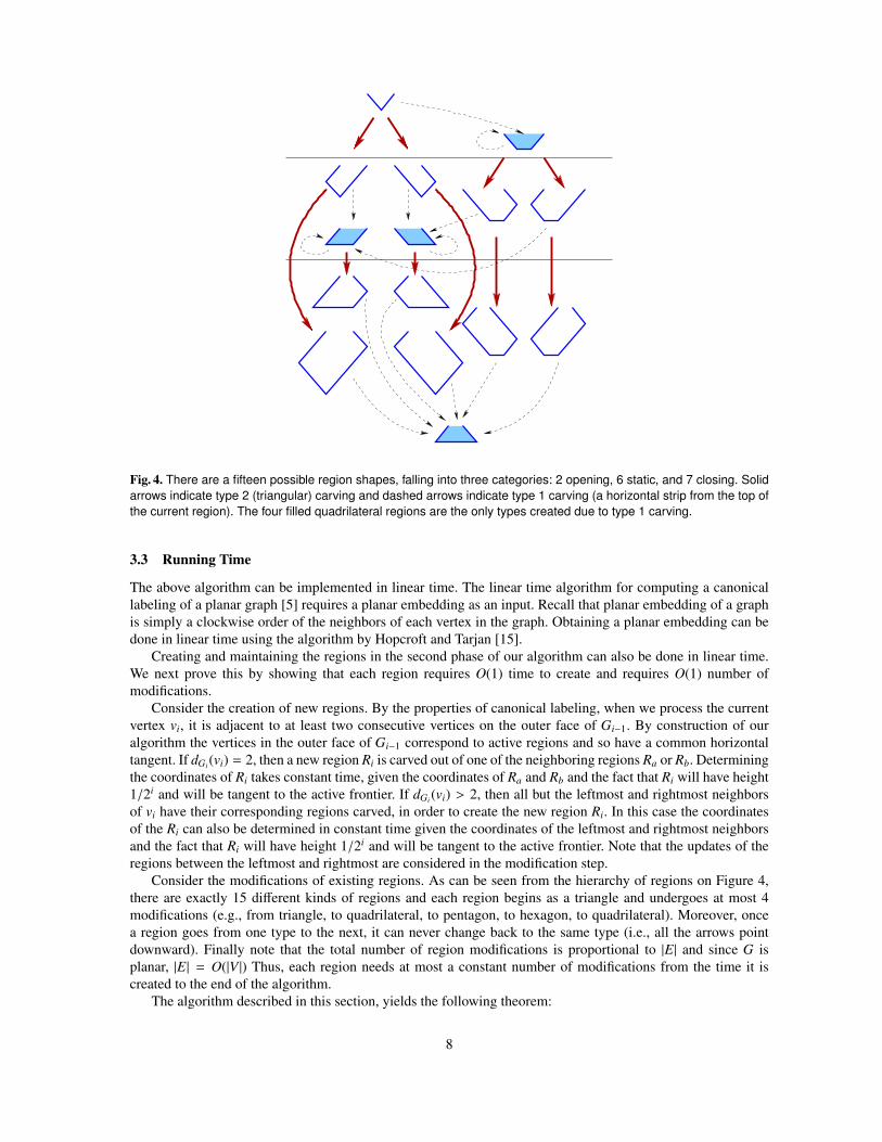
Fig. 4. There are a fifteen possible region shapes, falling into three categories: 2 opening, 6 static, and 7 closing. Solidarrows indicate type 2 (triangular) carving and dashed arrows indicate type 1 carving (a horizontal strip from the top ofthe current region). The four filled quadrilateral regions are the only types created due to type 1 carving.

3.3 Running Time

The above algorithm can be implemented in linear time. The linear time algorithm for computing a canonicallabeling of a planar graph [5] requires a planar embedding as an input. Recall that planar embedding of a graphis simply a clockwise order of the neighbors of each vertex in the graph. Obtaining a planar embedding can bedone in linear time using the algorithm by Hopcroft and Tarjan [15].

Creating and maintaining the regions in the second phase of our algorithm can also be done in linear time.We next prove this by showing that each region requires O(1) time to create and requires O(1) number ofmodifications.

Consider the creation of new regions. By the properties of canonical labeling, when we process the currentvertex vi, it is adjacent to at least two consecutive vertices on the outer face of Gi−1. By construction of ouralgorithm the vertices in the outer face of Gi−1 correspond to active regions and so have a common horizontaltangent. If dGi (vi) = 2, then a new region Ri is carved out of one of the neighboring regions Ra or Rb. Determiningthe coordinates of Ri takes constant time, given the coordinates of Ra and Rb and the fact that Ri will have height1/2i and will be tangent to the active frontier. If dGi (vi) > 2, then all but the leftmost and rightmost neighborsof vi have their corresponding regions carved, in order to create the new region Ri. In this case the coordinatesof the Ri can also be determined in constant time given the coordinates of the leftmost and rightmost neighborsand the fact that Ri will have height 1/2i and will be tangent to the active frontier. Note that the updates of theregions between the leftmost and rightmost are considered in the modification step.

Consider the modifications of existing regions. As can be seen from the hierarchy of regions on Figure 4,there are exactly 15 different kinds of regions and each region begins as a triangle and undergoes at most 4modifications (e.g., from triangle, to quadrilateral, to pentagon, to hexagon, to quadrilateral). Moreover, oncea region goes from one type to the next, it can never change back to the same type (i.e., all the arrows pointdownward). Finally note that the total number of region modifications is proportional to |E| and since G isplanar, |E| = O(|V |) Thus, each region needs at most a constant number of modifications from the time it iscreated to the end of the algorithm.

The algorithm described in this section, yields the following theorem:

8

Ra Rb

RiRa Rb

Ri

Ra Rb

RiRa Rb

RiRa Rb

Ri

Fig. 5. Introducing region Ri between Ra and Rb, assuming Ri is carved out of Ra. All the possible cases are shown,assuming that Ra and Rb were convex, at most 6-sided regions with slopes 0, 1, -1. (There are five more symmetriccases when Ri is carved out of Rb.) Note that these five regions correspond to the non-filled regions from the region-creating hierarchy in Fig. 4 with two static regions in the first row and the three closing regions in the second row.

Theorem 3. A planar graph can be converted into a set of touching convex polygons with complexity at mostsix, in linear time in the number of vertices of the graph.

As defined, the above algorithm requires exponential area, if polygonal endpoints are to be placed at integergrid points. We show in the Appendix how to compact the initial exponential area drawings. However, thecompaction approach is not guaranteed to always find a small area drawing. Therefore, we next show with adifferent algorithm that, in fact, O(n) × O(n) area suffices.

4 Hexagonal Representation of Planar Graphs using O(n) × O(n) Area

One drawback to the algorithms described in Sections 3 is it is not easy to obtain a good bound on the drawingarea. Using a different approach, we can show that any general n-vertex planar graph can be represented bytouching convex hexagons, drawn on the O(n) × O(n) grid. This approach is based on Kant’s algorithm forhexagonal grid drawing of 3-connected, 3-planar graphs [17]. In Kant’s algorithm the drawing is obtained bylooking at the dual graph, and processing its vertices in the canonical order. In the final drawing, however,there are two non-convex faces, separated by an edge which is not drawn as a straight-line segment. Theseproblems can be addressed by pre-processing the graph, by adding several extra vertices. When the dual of thisaugmented graph is embedded, the faces corresponding to the extra vertices can be removed to yield the desiredgrid drawing on area O(n) × O(n).

Let H = (V, E) be a 3-connected, 3-planar graph. Note that the dual D(H) is fully triangulated, as each facein the dual corresponds to exactly one vertex in H. So, for f faces in H, we have f vertices in D(H). We firstcompute a canonical ordering on the vertices of D(H) as defined by de Fraysseix et al. [7]. Let v1, ..., v f be thevertices in D(H) in this canonical order.

Kant’s algorithm now constructs a drawing for H such that all edges but one have slopes 0◦, 60◦, or −60◦,with the one edge with bends lying on the outer face. The typical structure of those drawings is shown inFigure 6(a).

The algorithm incrementally constructs the drawing by adding the faces of H in reverse order of the canoni-cal order of the corresponding vertices in D(H). We let wi be the vertices of H. Let face Fi correspond to vertexvi in D(H). The algorithm starts with a triangular region for the face F f that corresponds to vertex v f . The vertexwx which is adjacent to F f , F1 and F2 is placed at the bottom. Let wy and wz be the neighbors of wx in F f . Thesethree vertices form the corners of the first face F f . (wx,wz) and (wx,wy) are drawn upward with equal lengthsand slopes -1 and 1, respectively. All the edges on the path between wy and wz along F f are drawn horizontallybetween the two vertices. From this first triangle, all other faces are added in reverse canonical order to the upperboundary of the drawing region. If a face is completed by only one vertex wi, this vertex is placed appropriatelyabove the upper boundary such that it can be connected by two edges with slopes -1 and 1, respectively. If theface is completed by a path, then the two end segments of the path have slopes -1 and 1, while the other edges

9

G

a

b

x

z

y

c

F1

F2

Ff

(a) (b)

Fig. 6. (a) Polygonal structure obtain from Kant’s algorithm. (b) Graph G augmented by vertices z, y and x together withits dual which serves as input graph for Kant’s algorithm.

are horizontal. The construction ends when w1 is inserted, corresponding to the outer face F1. Note that there isan edge between w1 and wx, which is drawn using some bends. This edge is adjacent to the faces F1 (the outerface) and F2.

From this construction, we can observe that the angles at faces F f , ..., F3 have size ≤ π as the first two edgesdo not enter the vertex from above, and the last edge leaves the vertex upwards. Hence, we have the followingresult.

Lemma 5. The faces F f , ..., F3 are convex, and as the slopes of the edges are -1,0 or 1, they are drawn with atmost 6 sides.

This property is exactly what we are aiming for, as the vertices of our input graph G should be representedby convex regions of at most 6 sides. Unfortunately, Kant’s algorithm creates two non-convex faces F1 and F2separated by an edge which is not drawn as a line segment. Furthermore, the face F f is drawn as large as all theremaining faces F3, ...F f−1 together.

Kant also gave an area estimate for the result of his algorithm. A corollary of Kant’s algorithm is the follow-ing.

Corollary 1. For a given 3-connected, 3-planar graph H of n vertices, H − wx can be drawn within an area ofn/2 − 1 × n/2 − 1.

4.1 From Hexagonal Grid Drawing to Touching Hexagons

To apply Kant’s result to the problem of constructing touching hexagons representation, we enlarge the embed-ded input graph G so that the dual of the resulting graph G′ can be drawn using Kant’s algorithm in such a waythat the original vertices of G correspond to the faces F3, ..., F f−1.

We have to add 3 vertices which will correspond to the faces F1, F2 and F f in Kant’s algorithm. Since G isfully triangulated, let a, b and c be the vertices at the outer face of G in clockwise order. We add the vertices x, yand z in the outer face and connect toG appropriately. We want z to correspond to the outer face F1, y correspondto F2 and x to F f . First, we add x and connect it to a, b and c such that b and c are still in the outer face. Then

10

we add y and connect it to x, b and c such that b is still in the outer face. Finally, we add z and connect it to x, band c such that z, y and x are now in outer face, as shown in the Figure 6(b).

Since the vertices x, y, z are on the outer face, we can choose which one is first, second and last in thecanonical order. We can then apply Kant’s algorithm with the canonical order v1 = z, v2 = y and v f = x. Afterconstructing the final drawing, we remove the regions corresponding to vertices z, y and x, leaving us with ahexagonal representation of G. Since Kant’s algorithm runs in linear time, and our emendations can be done inconstant time, we can summarize:

Theorem 4. For a fully triangulated planar graph G on n vertices, we can construct a contact graph of convexhexagons in time O(n). The sides of the hexagons have slope 1, 0, or -1.

Given any planar graph G, if it is not biconnected, we can make it biconnected using a procedure attributed toRead [27], adding a vertex and two edges at each articulation point. Once biconnected, we can fully triangulatethe graph by adding a vertex inside each non-triangular face and connecting that vertex to each vertex on theface. We can then apply Theorem 4, to get a hexagonal representation of the extended graph. Finally, removingthe added vertices and their edges, we obtain a hexagonal representation of G. This gives us:

Theorem 5. For any planar graph G on n vertices, we can construct a contact graph of convex hexagons intime O(n). The sides of the hexagons have slope 1, 0, or -1.

4.2 Area estimation

For a triangulated input graph G = (V, E), we have n vertices and, by Euler’s formula, 2n − 4 faces. Since weenhanced our graph to n + 3 vertices, we have f = 2n + 2 faces. Those faces are the vertices in the dual D(G)which is the input to Kant’s algorithm. His area estimation gives an area of n/2 − 1 × n/2 − 1 for f = n verticeswhen we coalesce the faces F1, F2 and F f into a single outer face by removing the corresponding vertices andedges. Thus, we get an area bound of n × n using exactly the same argument as he did.

Theorem 6. For a fully triangulated planar graph G of n vertices, we can achieve a contact representation ofconvex hexagons with area n × n.

5 Conclusion and Future Work

Thomassen [29] had shown that not all planar graphs can be represented by touching pentagons, where theexternal boundary of the figure is also a pentagon and there are no holes between pentagons. Our results in thispaper are more general, as we do not insist on the external boundary being a pentagon or on there being no holesbetween pentagons. Finally, it is possible to derive algorithms for convex hexagonal representations for generalplanar graphs from several earlier papers, e.g., de Fraysseix et al. [7], Thomassen [29], and Kant [17]. However,the work of Thomassen, Kant, and de Fraysseix et al. does not immediately lead to algorithmic solutions to theproblem of touching polygons graph representation with convex low-complexity polygons. To the best of ourknowledge, this problem has never been formally considered or described.

In this paper we presented several results about touching n-sided graphs. We showed that for general planargraph six sides are necessary. Then we presented an algorithm for representing general planar graphs withconvex hexagons. Finally, we discussed a different algorithm for general planar graphs which also yields anO(n) × O(n) drawing area.

Several interesting related problems are open. What is the complexity of the deciding whether a given pla-nar graph can be represented by touching triangles, quadrilaterals, or pentagons? In the context of rectilinearcatrograms the vertex-weighted problem has been carefully studied. However, the same problem without therectilinear constraint has received less attention. Finally, it would be interesting to characterize the subclasses ofplanar graphs that allow for touching triangles, touching quadrilaterals, and touching pentagons representations.

6 Acknowledgments

We would like to thank Therese Biedl for pointing out the very relevant work by Kant and Thomassen.

11

References

1. G. D. Battista, W. Lenhart, and G. Liotta. Proximity drawability: A survey. In Proc. Graph Drawing, volume 894 ofLecture Notes in Computer Science, pages 328–39. Springer-Verlag, 1994.

2. T. Biedl, A. Bretscher, and H. Meijer. Rectangle of influence drawings of graphs without filled 3-cycles. In Proc. 7thInt’l. Symp. on Graph Drawing ’99, pages 359–368, 1999.

3. M. Bruls, K. Huizing, and J. J. van Wijk. Squarified treemaps. In Proc. Joint Eurographics/IEEE TVCG Symp. Visual-ization, VisSym, pages 33–42, 2000.

4. A. L. Buchsbaum, E. R. Gansner, C. M. Procopiuc, and S. Venkatasubramanian. Rectangular layouts and contact graphs.ACM Transactions on Algorithms, 4(1), 2008.

5. M. Chrobak and T. Payne. A linear-time algorithm for drawing planar graphs. Inform. Process. Lett., 54:241–246, 1995.6. M. de Berg, E. Mumford, and B. Speckmann. On rectilinear duals for vertex-weighted plane graphs. Discrete Mathe-

matics, 309(7):1794–1812, 2009.7. H. de Fraysseix, P. O. de Mendez, and P. Rosenstiehl. On triangle contact graphs. Combinatorics, Probability and

Computing, 3:233–246, 1994.8. H. de Fraysseix, J. Pach, and R. Pollack. Small sets supporting Fary embeddings of planar graphs. In Procs. 20th

Symposium on Theory of Computing (STOC), pages 426–433, 1988.9. H. de Fraysseix, J. Pach, and R. Pollack. How to draw a planar graph on a grid. Combinatorica, 10(1):41–51, 1990.

10. K. R. Gabriel and R. R. Sokal. A new statistical approach to geographical analysis. Systematic Zoology, 18:54–64,1969.

11. X. He. On finding the rectangular duals of planar triangular graphs. SIAM Journal of Computing, 22(6):1218–1226,1993.

12. X. He. On floor-plan of plane graphs. SIAM Journal of Computing, 28(6):2150–2167, 1999.13. P. Hlineny. Classes and recognition of curve contact graphs. Journal of Comb. Theory (B), 74(1):87–103, 1998.14. P. Hlineny and J. Kratochvıl. Representing graphs by disks and balls (a survey of recognition-complexity results).

Discrete Mathematics, 229(1-3):101–24, 2001.15. J. Hopcroft and R. E. Tarjan. Efficient planarity testing. Journal of the ACM, 21(4):549–568, 1974.16. J. W. Jaromczyk and G. T. Toussaint. Relative neighborhood graphs and their relatives. Proceedings of the IEEE,

80:1502–17, 1992.17. G. Kant. Hexagonal grid drawings. In 18th Workshop on Graph-Theoretic Concepts in Computer Science, pages

263–276, 1992.18. G. Kant. Drawing planar graphs using the canonical ordering. Algorithmica, 16:4–32, 1996. (special issue on Graph

Drawing, edited by G. Di Battista and R. Tamassia).19. G. Kant and X. He. Regular edge labeling of 4-connected plane graphs and its applications in graph drawing problems.

Theoretical Computer Science, 172:175–93, 1997.20. P. Koebe. Kontaktprobleme der konformen Abbildung. Berichte uber die Verhandlungen der Sachsischen Akademie

der Wissenschaften zu Leipzig. Math.-Phys. Klasse, 88:141–164, 1936.21. K. Kozminski and W. Kinnen. Rectangular dualization and rectangular dissections. IEEE Transactions on Circuits and

Systems, 35(11):1401–16, 1988.22. Y.-T. Lai and S. M. Leinwand. Algorithms for floorplan design via rectangular dualization. IEEE Transactions on

Computer-Aided Design, 7:1278–89, 1988.23. Y.-T. Lai and S. M. Leinwand. A theory of rectangular dual graphs. Algorithmica, 5:467–83, 1990.24. C.-C. Liao, H.-I. Lu, and H.-C. Yen. Compact floor-planning via orderly spanning trees. Journal of Algorithms, 48:441–

451, 2003.25. G. Liotta, A. Lubiw, H. Meijer, and S. H. Whitesides. The rectangle of influence drawability problem. Computational

Geometry: Theory and Applications, 10:1–22, 1998.26. M. Rahman, T. Nishizeki, and S. Ghosh. Rectangular drawings of planar graphs. Journal of Algorithms, 50(1):62–78,

2004.27. R. C. Read. A new method for drawing a graph given the cyclic order of the edges at each vertex. Congressus

Numerantium, 56:31–44, 1987.28. P. Steadman. Graph-theoretic representation of architectural arrangement. In L. March, editor, The Architecture of

Form, pages 94–115. Cambridge University Press, 1976.29. C. Thomassen. Plane representations of graphs. In J. A. Bondy and U. S. R. Murty, editors, Progress in Graph Theory,

pages 43–69, 1982.30. C. Thomassen. Interval representations of planar graphs. Journal of Comb. Theory (B), 40:9–20, 1988.31. G. K. Yeap and M. Sarrafzadeh. Sliceable floorplanning by graph dualization. SIAM Journal on Discrete Mathematics,

8(2):258–80, 1995.

12

A Compact Grid Drawings

Figure A shows several examples of planar graphs and the corresponding output from our algorithm after acompaction step which minimizes the required integer grid.

Fig. 7. Examples illustrating input graphs and the corresponding plane partitions.

The algorithm given in Section 3.2 provides a touching hexagons representation of any planar graph. Theincremental process carves out polygons within an ever smaller band of active front, therefore in practice thedrawing is highly skewed. In this section we describe an algorithm to get a drawing on the grid.

13

It is easy to see that when looking at the vertices and edges created in the algorithm for touching hexagons,if the horizontal edges are ignored, then the resulting graph is a “binary” tree, in the sense that each node hasa degree of no more than 2. To achieve a drawing on the grid, we employ a divide and conquer algorithm. Weneed each edge to be of either 45 or -45 degree relative to the x axes, and that we have to constrain verticeslinked by the omitted horizontal edges to the same y-coordinates.

Let GT6G be the graph derived from the touching hexagons algorithm. Define a cap as a maximal connectedcomponent of vertices and horizontal edges of GT6G. After removing the edges in the caps from GT6G, theremaining graph GT is a binary tree.

Define the frontal vertex set F of a tree as the set of leaf vertices, such that if a vertex in this set is also in acap, then all the vertices in the same cap must also be leaves. This means that if a vertex that belongs to a capis in the front, every vertex in this cap is also in the front. We initialize the current tree to be Gc = GT , and thehorizontal shift of every vertex to 0.

– 1. Let F be the frontal vertex set of Gc. If F is empty, exit.– 2. For each vertex v in the front F,• if v is a leaf in GT , place v on at x = 0 and y = 0.• if v has one subtree in GT , say to the right, extend a line of 45 degree from the root of this right subtree

by 1 unit down and left to get the position of v.• if v has two subtrees in GT , shift the right subtree horizontally so that the two subtrees have a separation

of either distance 1 or 2, and the line of -45 degree from the root of the left subtree and the line of 45degree from the root of the right subtree meet at a grid point. Record this position of v, and the shift atthe root of the right tree.

– 3. For each cap C in the front, set h to be the maximum of the absolute values of y coordinates of verticesin C. For every vertex v ∈ C,• if the y(v) > −h, set y(v) = −h if v has no subtrees in GT . Otherwise, by construction, vertex v must have

only one subtree, say to the right. Extend the 45 degree line from the root of the subtree till it intersectswith line y = −h, record the coordinates of the intersection point as the coordinates for v.

– 4. Delete F and its connecting edges from GC , renaming the resulting tree GC . Go to Step 1.

At the end of this algorithm, each vertex of GT has x−, y− coordinates and a horizontal shift. A traversal fromthe root is carried out to propagate the shifts and to get the final position of every vertex. This gives a drawing ofthe GT6G on a grid. Figure A shows several graphs, and their corresponding touching hexagons representationson a grid.

14