International Journal of Bifurcation and Chaos, Vol. 17, No. 7 (2007) 2215–2255 c World Scientific Publishing Company OPTIMAL PATH AND MINIMAL SPANNING TREES IN RANDOM WEIGHTED NETWORKS LIDIA A. BRAUNSTEIN ∗,† , ZHENHUA WU † , YIPING CHEN † , SERGEY V. BULDYREV †,‡ , TOMER KALISKY § , SAMEET SREENIVASAN † , REUVEN COHEN §,¶ , EDUARDO L ´ OPEZ †,∗∗ , SHLOMO HAVLIN †,§ and H. EUGENE STANLEY † ∗ Departamento de F´ ısica, Facultad de Ciencias Exactas y Naturales, Universidad Nacional de Mar del Plata, Funes 3350, 7600 Mar del Plata, Argentina † Center for Polymer Studies, Boston University, Boston, MA 02215, USA ‡ Department of Physics Yeshiva University, 500 West 185th Street Room 1112, NY 10033, USA § Minerva Center and Department of Physics, Bar-Ilan University, 52900 Ramat-Gan, Israel ¶ Department of Electrical and Computer Engineering, Boston University, Boston, MA 02215, USA ∗∗ Theoretical Division, Los Alamos National Laboratory, Mail Stop B258, Los Alamos, NM 87545, USA ∗ [email protected] Received May 20, 2006; Revised September 22, 2006 We review results on the scaling of the optimal path length opt in random networks with weighted links or nodes. We refer to such networks as “weighted” or “disordered” networks. The optimal path is the path with minimum sum of the weights. In strong disorder, where the maximal weight along the path dominates the sum, we find that opt increases dramatically compared to the known small-world result for the minimum distance min ∼ log N , where N is the number of nodes. For Erd˝ os–R´ enyi (ER) networks opt ∼ N 1/3 , while for scale free (SF) networks, with degree distribution P (k) ∼ k −λ , we find that opt scales as N (λ−3)/(λ−1) for 3 <λ< 4 and as N 1/3 for λ ≥ 4. Thus, for these networks, the small-world nature is destroyed. For 2 <λ< 3 in contrary, our numerical results suggest that opt scales as ln λ−1 N , representing still a small world. We also find numerically that for weak disorder opt ∼ ln N for ER models as well as for SF networks. We also review the transition between the strong and weak disorder regimes in the scaling properties of opt for ER and SF networks and for a general distribution of weights τ , P (τ ). For a weight distribution of the form P (τ )=1/(aτ ) with (τ min <τ<τ max ) and a = ln τ max /τ min , we find that there is a crossover network size N ∗ = N ∗ (a) at which the transition occurs. For N N ∗ the scaling behavior of opt is in the strong disorder regime, while for N N ∗ the scaling behavior is in the weak disorder regime. The value of N ∗ can be determined from the expression ∞ (N ∗ )= ap c , where ∞ is the optimal path length in the limit of strong disorder, A ≡ ap c →∞ and p c is the percolation threshold of the network. We suggest that for any P (τ ) the distribution of optimal path lengths has a universal form which is controlled by the scaling parameter Z = ∞ /A where A ≡ p c τ c / τc 0 τP (τ )dτ plays the role of the 2215

Welcome message from author
This document is posted to help you gain knowledge. Please leave a comment to let me know what you think about it! Share it to your friends and learn new things together.
Transcript
International Journal of Bifurcation and Chaos, Vol. 17, No. 7 (2007) 2215–2255c© World Scientific Publishing Company
OPTIMAL PATH AND MINIMAL SPANNINGTREES IN RANDOM WEIGHTED NETWORKS
LIDIA A. BRAUNSTEIN∗,†, ZHENHUA WU†, YIPING CHEN†,SERGEY V. BULDYREV†,‡, TOMER KALISKY§,SAMEET SREENIVASAN†, REUVEN COHEN§,¶,EDUARDO LOPEZ†,∗∗, SHLOMO HAVLIN†,§ and
H. EUGENE STANLEY†∗Departamento de Fısica,
Facultad de Ciencias Exactas y Naturales,Universidad Nacional de Mar del Plata,
Funes 3350, 7600 Mar del Plata, Argentina†Center for Polymer Studies, Boston University,
Boston, MA 02215, USA‡Department of Physics Yeshiva University,
500 West 185th Street Room 1112, NY 10033, USA§Minerva Center and Department of Physics,Bar-Ilan University, 52900 Ramat-Gan, Israel
¶Department of Electrical and Computer Engineering,Boston University, Boston, MA 02215, USA
∗∗Theoretical Division, Los Alamos National Laboratory,Mail Stop B258, Los Alamos, NM 87545, USA
Received May 20, 2006; Revised September 22, 2006
We review results on the scaling of the optimal path length �opt in random networks withweighted links or nodes. We refer to such networks as “weighted” or “disordered” networks.The optimal path is the path with minimum sum of the weights. In strong disorder, where themaximal weight along the path dominates the sum, we find that �opt increases dramaticallycompared to the known small-world result for the minimum distance �min ∼ log N , where Nis the number of nodes. For Erdos–Renyi (ER) networks �opt ∼ N1/3, while for scale free (SF)networks, with degree distribution P (k) ∼ k−λ, we find that �opt scales as N (λ−3)/(λ−1) for3 < λ < 4 and as N1/3 for λ ≥ 4. Thus, for these networks, the small-world nature is destroyed.For 2 < λ < 3 in contrary, our numerical results suggest that �opt scales as lnλ−1 N , representingstill a small world. We also find numerically that for weak disorder �opt ∼ ln N for ER modelsas well as for SF networks. We also review the transition between the strong and weak disorderregimes in the scaling properties of �opt for ER and SF networks and for a general distributionof weights τ , P (τ). For a weight distribution of the form P (τ) = 1/(aτ) with (τmin < τ < τmax)and a = ln τmax/τmin, we find that there is a crossover network size N∗ = N∗(a) at which thetransition occurs. For N � N∗ the scaling behavior of �opt is in the strong disorder regime,while for N � N∗ the scaling behavior is in the weak disorder regime. The value of N∗ canbe determined from the expression �∞(N∗) = apc, where �∞ is the optimal path length in thelimit of strong disorder, A ≡ apc → ∞ and pc is the percolation threshold of the network. Wesuggest that for any P (τ) the distribution of optimal path lengths has a universal form which iscontrolled by the scaling parameter Z = �∞/A where A ≡ pcτc/
∫ τc
0 τP (τ)dτ plays the role of the
2215
2216 L. A. Braunstein et al.
disorder strength and τc is defined by∫ τc
0 P (τ)dτ = pc. In case P (τ) ∼ 1/(aτ), the equation forA is reduced to A = apc. The relation for A is derived analytically and supported by numericalsimulations for Erdos–Renyi and scale-free graphs. We also determine which form of P (τ) canlead to strong disorder A → ∞. We then study the minimum spanning tree (MST), which is thesubset of links of the network connecting all nodes of the network such that it minimizes thesum of their weights. We show that the minimum spanning tree (MST) in the strong disorderlimit is composed of percolation clusters, which we regard as “super-nodes”, interconnectedby a scale-free tree. The MST is also considered to be the skeleton of the network where themain transport occurs. We furthermore show that the MST can be partitioned into two distinctcomponents, having significantly different transport properties, characterized by centrality —number of times a node (or link) is used by transport paths. One component the superhighways,for which the nodes (or links) with high centrality dominate, corresponds to the largest clusterat the percolation threshold (incipient infinite percolation cluster) which is a subset of the MST.The other component, roads, includes the remaining nodes, low centrality nodes dominate. Wefind also that the distribution of the centrality for the incipient infinite percolation clustersatisfies a power law, with an exponent smaller than that for the entire MST. We demonstratethe significance identifying the superhighways by showing that one can improve significantly theglobal transport by improving a very small fraction of the network, the superhighways.
Keywords : Minimum spanning tree; percolation; scale-free; optimization.
1. Introduction
Recently much attention has been focused onthe topic of complex networks which characterizemany biological, social, and communication sys-tems [Albert & Barabasi, 2002; Mendes et al., 2003;Pastor-Satorras & Vespignani, 2004]. The networksare represented by nodes associated to individu-als, organizations, or computers and by links rep-resenting their interactions. The classical model forrandom networks is the Erdos–Renyi (ER) model[Erdos & Renyi, 1959, 1960; Bollobas, 1985]. Animportant quantity characterizing networks is theaverage distance (minimal hopping) �min betweentwo nodes in the network of total N nodes. Forthe Erdos–Renyi network �min scales as ln N [Bol-lobas, 1985], which leads to the concept of “smallworlds” or “six degrees of separation”. For scale-free(SF) [Albert & Barabasi, 2002] networks �min scalesas ln ln N , this leads to the concept of ultra smallworlds [Cohen et al., 2002; Mendes et al., 2003].
In most studies, all links in the network areregarded as identical and thus a crucial parame-ter for information flow including efficient routing,searching and transport is �min. In practice, how-ever, the weights (e.g. the quality or cost) of linksare usually not equal [Barrat et al., 2004; Boccalettiet al., 2006].
Thus the length of the optimal path �opt, min-imizing the sum of weights, is usually longer than
�min. For example, the cost could be the timerequired to transit the link. There are often manytraffic routes from site A to site B with a set oftransit time τi, associated with each link along thepath. The fastest (optimal) path is the one for which∑
i τi is a minimum, and often the optimal pathhas more links than the shortest path. In manycases, the selection of the path is controlled by mostof the weights (e.g. total cost) contributing to thesum. This case corresponds to weak disorder (WD).However, in other cases, for example when the dis-tribution of disorder is very broad a single weightdominates the sum. This situation — in which onelink controls the selection of the path — is calledthe strong disorder limit (SD).
For a recent quantitative criterion for SD andWD, see [Chen et al., 2006] and Sec. 4.2 in thisarticle.
The strong disorder is relevant e.g. for com-puter and traffic networks, since the slowest link incommunication networks determines the connectionspeed. An example for SD is when a transmissionat a constant high rate is needed (e.g. in broadcast-ing video records over the Internet). In this casethe narrowest band link in the path between thetransmitter and receiver controls the rate of trans-mission. This limit is also called the “ultrametric”limit and we refer to the optimal path in this limitas the min-max path.
Optimal Path and Minimal Spanning Trees in Random Weighted Networks 2217
The SD limit is also related to the minimalspanning tree which includes all optimal pathsbetween all pairs of sites in the network. The disor-der on a network is usually implemented from a dis-tribution P (τ) ∼ 1/(aτ), where 1 < τ < ea [Portoet al., 1999; Braunstein et al., 2001; Cieplak et al.,1996; Braunstein et al., 2003]. We assign to eachlink of the network a random number r, uniformlydistributed between 0 and 1. The cost associatedwith link i is then τi ≡ exp(ari) where a is theparameter which controls the broadness of the dis-tribution of link costs. The parameter a representsthe strength of disorder. The limit a → ∞ is thestrong disorder limit, since for this case clearly onlyone link dominates the cost of the path. The strongdisorder limit (SD) can be implemented in a disor-dered media by assigning to each link a potentialbarrier εi so that τi is the time to cross this barrierin a thermal activation process. Thus τi = eεi/KT ,where K is the Boltzmann constant and T is abso-lute temperature. The optimal path corresponds tothe minimum (
∑i τi) over all possible paths. We can
define disorder strength a = 1/KT . When a → ∞,only the largest τi dominates the sum. Thus, T → 0(very low temperature) corresponds to the strongdisorder limit.
There are distinct scaling relationships betweenthe length of the average optimal path �opt andthe network size (number of nodes) N depend-ing on whether the network is strongly or weaklydisordered [Porto et al., 1999; Braunstein et al.,2003]. It was shown using percolation arguments(see Sec. 4) that for strong disorder [Braunsteinet al., 2003], �opt ∼ Nνopt , where νopt = 1/3for Erdos–Renyi (ER) random networks [Erdos &Renyi, 1959] and for scale-free (SF) [Albert &Barabasi, 2002] networks with λ > 4, where λ isthe exponent characterizing the power law decayof the degree distribution. For SF networks with3 < λ < 4, νopt = (λ − 3)/(λ − 1). For 2 <λ < 3, percolation arguments do not work, butthe numerical results suggest �opt ∼ lnλ−1 N , whichis again much larger than the ultra small resultfor the shortest path �min ∼ ln ln N found for2 < λ < 3 in [Cohen & Havlin, 2003]. Whenthe weights are taken from a uniform distribu-tion we are in the weak disorder limit. In thiscase �opt ∼ ln N for both ER and SF for allvalues of λ [Braunstein et al., 2003]. For 2 <λ < 3, this result is significantly different fromthe ultra small-world result found for unweighednetworks.
Porto [Porto et al., 1999] considered the opti-mal path transition from weak to strong disorderfor 2-D and 3-D lattices, and found a crossoverin the scaling properties of the optimal path thatdepends on the disorder strength a, as well as thelattice size L (see also [Buldyrev et al., 2006]). Sim-ilar to regular lattices, there exists for any finitea, a crossover network size N∗(a) such that forN � N∗(a), the scaling properties of the optimalpath are in the strong disorder regime while forN � N∗(a), the network is in the weak disorderregime. The function N∗(a) was evaluated. More-over, a general criterion to determine which formof P (τ) can lead to strong disorder, and a generalcondition when strong or weak disorder occurs wasfound analytically [Chen et al., 2006]. The deriva-tion was supported by extensive simulations.
The study of the distribution of the lengthof the optimal paths in a network was reportedin [Kalisky et al., 2005]. It was found that thedistribution has the scaling form P (�opt, N, a) ∼(1/�∞)G(�opt/�∞, (1/pc)(�∞/a)), where �∞ is �opt
for a → ∞ and pc is the percolation threshold.It was also shown that a single parameter Z ≡(1/pc)(�∞/a) determines the functional form of thedistribution. Importantly, it was found [Chen et al.,2006] that for all P (τ) that possess a strong-weakdisorder crossover, the distributions P (�opt) of theoptimal path lengths display the same universalbehavior.
Another interesting question is about a pos-sible origin of scale-free degree distribution withλ = 2.5 in some real world networks. Kalisky[Kalisky et al., 2006] introduced a simple processthat generates random scale-free networks with λ =2.5 from weighted Erdos–Renyi graphs [Erdos &Renyi, 1960]. They found that the minimum span-ning tree (MST) on an Erdos–Renyi graph is com-posed of percolation clusters, which we regard as“super nodes”, interconnected by a scale-free treewith λ = 2.5.
Known as the tree with the minimum weightamong all possible spanning tree, the MST is alsothe union of all “strong disorder” optimal pathsbetween any two nodes [Barabasi, 1996; Dobrin &Duxbury, 2001; Cieplak et al., 1996; Porto et al.,1999; Braunstein et al., 2003; Wu et al., 2005]. Asthe global optimal tree, the MST plays a majorrole for transport process, which is widely usedin different fields, such as the design and oper-ation of communication networks, the travelingsalesman problem, the protein interaction problem,
2218 L. A. Braunstein et al.
optimal traffic flow, and economic networks [Khanet al., 2003; Skiena, 1990; Fredman & Tarjan, 1987;Kruskal, 1956; Macdonald et al., 2005; Bonannoet al., 2003; Onnela et al., 2003]. One importantquestion in network transport is how to identify thenodes or links that are more important than others.A relevant quantity that characterizes transport innetworks is the betweenness centrality, C, which isthe number of times a node (or link) used by alloptimal paths between all pairs of nodes [Newman,2001a, 2001b; Goh et al., 2001; Kim et al., 2004].For simplicity we call the “betweenness centrality”here “centrality” and we use the notation “nodes”but similar results have been obtained for links. Thecentrality, C, quantifies the “importance” of a nodefor transport in the network. Moreover, identify-ing the nodes with high C enables us to improvetheir transport capacity and thus improve the globaltransport in the network. The probability densityfunction (pdf) of C was studied on the MST forboth SF [Barabasi & Albert, 1999] and ER [Erdos& Renyi, 1959, 1960] networks and found to sat-isfy a power law, PMST(C) ∼ C−δMST , with δMST
close to 2 [Goh et al., 2005; Kim et al., 2004]. How-ever, [Wu et al., 2006] found that a sub-network ofthe MST,1 the infinite incipient percolation cluster(IIC) has a significantly higher average C than theentire MST — i.e. the set of nodes inside the IICare typically used by transport paths more oftenthan other nodes in the MST (see Sec. 9). In thissense the IIC can be viewed as a set of superhigh-ways (SHW) in the MST. The nodes on the MSTwhich are not in the IIC are called roads, due totheir analogy with roads which are not superhigh-ways (usually used by local residents). Wu et al.[2006] demonstrated the impact of this finding byshowing that improving the capacity of the super-highways (IIC) is significantly a better strategy toenhance global transport compared to improvingthe same number of links of the highest C in theMST, although they have higher C.2 This counter-intuitive result shows the advantage of identifyingthe IIC subsystem, which is very small and of orderzero compared to the full network.3
2. Algorithms
2.1. Construction of the networks
To construct an ER network of size N with averagenode degree 〈k〉, we start with 〈k〉N/2 edges andrandomly pick a pair of nodes from the total possi-ble N(N − 1)/2 pairs to connect with an edge. Theonly condition we impose is that there cannot bemultiple edges between two nodes. When 〈k〉 > 1almost all nodes of the network will be connectedwith high probability.
To generate scale-free (SF) graphs of size N , weemploy the Molloy–Reed algorithm [Molloy & Reed,1998]. Initially the degree of each node is chosenaccording to a scale-free distribution, where eachnode is given a number of open links or “stubs”according to its degree. Then, stubs from all nodesof the network are interconnected randomly to eachother with two constraints that there are no multi-ple edges between two nodes and that there are nolooped edges with identical ends. The exact form ofthe degree distribution is usually taken to be
P (k) = ck−λ k = m, . . . ,K (1)
where m and K are the minimal and maximaldegrees, and c ≈ (λ − 1)mλ−1 is a normaliza-tion constant. For real networks with finite size,the highest degree K depends on network size N :K ≈ mN1/(λ−1), thus creating a “natural” cut-off for the highest possible degree. When m > 1there is a high probability that the network is fullyconnected.
2.2. Dijkstra’s algorithm
The Dijkstra’s algorithm [Cormen et al., 1990] isused in general to find the optimal path, when theweights are drawn from an arbitrary distribution.The search for the optimal path follows a procedureakin to “burning” where the “fire” starts from ourchosen origin. At the beginning, all nodes are givena distance ∞ except the origin which is given a dis-tance 0. At each step we choose the next unburned
1The IIC contains loops in lattices in dimension d below 6. However, for networks (d = ∞), in the IIC loops can be neglegtedand in this case for large N the IIC must be a subset of the MST. In our simulations, we found that more than 99% links ofIIC belong to MST. For lattices, we only choose the part of the IIC that belongs to the MST.2The overlap between the two groups is about 30% for ER networks of size N = 8192.3The ratio 〈NIIC/NMST〉 approaches zero for large NMST ≡ N due to the fractal nature of the IIC. Indeed, NIIC ∼ N2/3
both for ER [Erdos & Renyi, 1959] and for SF with λ > 4 [Cohen]. For SF with λ = 3.5, NIIC ∼ N0.6 [Cohen] and for the
L × L square lattice NIIC ∼ L91/48 ∼ N91/96 [Bunde & Havlin, 1996].
Optimal Path and Minimal Spanning Trees in Random Weighted Networks 2219
node which is nearest to the origin, and “burn” it,while updating the optimal distance to all its neigh-bors. The optimal distance of a neighbor is updatedonly if reaching it from the current burning nodegives a total path length that is shorter than itscurrent distance.
2.3. Ultrametric optimization
Next, we describe a numerical method for comput-ing �opt between any two nodes in strong disorder[Dobrin & Duxbury, 2001; Braunstein et al., 2001].In this case the sum of the weights must be com-pletely dominated by the largest weight. Sometimesthis condition is referred to as ultrametric. We cansatisfy this condition assigning weights to all thelinks τi = exp(ari) choosing a to be so large, thatany two links will have different binary orders ofmagnitude. For example, if we can select 0 ≤ ri < 1from a uniform distribution, using a 48-bit randomnumber generator, there will be no two identical val-ues of ri in a system of any size that we study. In thiscase ∆ri ≥ 2−48 and we can select a ≥ 248 ln 2 to
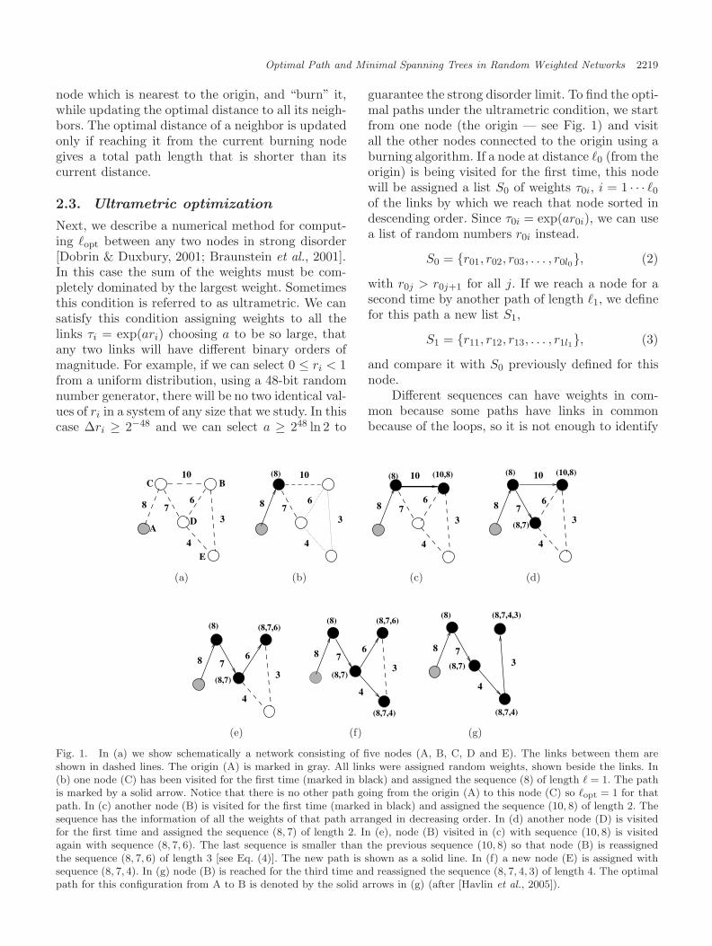
guarantee the strong disorder limit. To find the opti-mal paths under the ultrametric condition, we startfrom one node (the origin — see Fig. 1) and visitall the other nodes connected to the origin using aburning algorithm. If a node at distance �0 (from theorigin) is being visited for the first time, this nodewill be assigned a list S0 of weights τ0i, i = 1 · · · �0
of the links by which we reach that node sorted indescending order. Since τ0i = exp(ar0i), we can usea list of random numbers r0i instead.
S0 = {r01, r02, r03, . . . , r0l0}, (2)
with r0j > r0j+1 for all j. If we reach a node for asecond time by another path of length �1, we definefor this path a new list S1,
S1 = {r11, r12, r13, . . . , r1l1}, (3)
and compare it with S0 previously defined for thisnode.
Different sequences can have weights in com-mon because some paths have links in commonbecause of the loops, so it is not enough to identify
76
4
3
8
10
A
C B
D
E
7
4
3
10
8 6
(8) 10
6 7
4
3
8
(10,8) (8)
76
4
3
8
10
(8,7)
(8) (10,8)
(a) (b) (c) (d)
(8,7)
76
4
3
8
(8) (8,7,6)
76
4
3
8
(8,7)
(8) (8,7,6)
(8,7,4)
7
4
3
8
(8,7)
(8,7,4,3)(8)
(8,7,4)
(e) (f) (g)
Fig. 1. In (a) we show schematically a network consisting of five nodes (A, B, C, D and E). The links between them areshown in dashed lines. The origin (A) is marked in gray. All links were assigned random weights, shown beside the links. In(b) one node (C) has been visited for the first time (marked in black) and assigned the sequence (8) of length � = 1. The pathis marked by a solid arrow. Notice that there is no other path going from the origin (A) to this node (C) so �opt = 1 for thatpath. In (c) another node (B) is visited for the first time (marked in black) and assigned the sequence (10, 8) of length 2. Thesequence has the information of all the weights of that path arranged in decreasing order. In (d) another node (D) is visitedfor the first time and assigned the sequence (8, 7) of length 2. In (e), node (B) visited in (c) with sequence (10, 8) is visitedagain with sequence (8, 7, 6). The last sequence is smaller than the previous sequence (10, 8) so that node (B) is reassignedthe sequence (8, 7, 6) of length 3 [see Eq. (4)]. The new path is shown as a solid line. In (f) a new node (E) is assigned withsequence (8, 7, 4). In (g) node (B) is reached for the third time and reassigned the sequence (8, 7, 4, 3) of length 4. The optimalpath for this configuration from A to B is denoted by the solid arrows in (g) (after [Havlin et al., 2005]).
2220 L. A. Braunstein et al.
the sequence by its maximum weight; in this case itmust also be compared with the second maximum,the third maximum, etc. We define Sp < Sq if thereexists a value m, 1 ≤ m ≤ min(�p, �q) such that
rpj = rqj for 1 ≤ j < m andrpj < rqj for j = m,
(4)
or if �q > �p and rpj = rqj for all j ≤ �p. IfS1 < S0, we replace S0 by S1. The procedure con-tinues until all paths have been explored and com-pared. At this point, S0 = Sopt, where Sopt is thesequence of weights for the optimal path of length�opt. A schematic representation of this ultrametricalgorithm is presented in Fig. 1. This algorithm isslow and memory consuming since we have to keeptrack of a sequence of values and the rank. Usingthis method, we obtain systems of sizes up to 212
nodes, typically 105 realizations of disorder.
2.4. Bombing optimization
This algorithm allows to compute �opt (and otherrelevant quantities) between any two nodes instrong disorder limit and was introduced by Cieplaket al. [1996]. Basically the algorithm does thefollowing
1. Sort the edges by descending weight.2. If the removal of the highest weight edge will not
disconnect A from B — remove it.3. Go back to step 2 until all edges have been pro-
cessed.
Since the edge weights are random, so is the order-ing. Therefore, in fact, one does not need even toselect edge weights and “bombing” algorithm canbe simplified by removing randomly chosen edgesone at a time, provided that their removal does notbreak the connectivity between the two nodes. Thebottleneck of this algorithm is checking the connec-tivity after each removal. To speed it up, we firstcompute the minimal path between nodes A andB using Dijkstra’s algorithm. Then we must checkthe connectivity only if the removed bond belongsto this path. In this case, we attempt to compute anew minimal path between A and B on the subset ofremaining bonds. If our attempt fails, it means thatthe removal of this bond would destroy the connec-tivity between A and B. Therefore, we restore thisbond and exclude it from the list of bonds subject torandom removal. With this improvement we couldreach systems of sizes up to 216 nodes and 105 real-izations of weight disorder.
2.5. The minimum spanningtree (MST )
The MST on a weighted graph is a tree thatreaches all nodes of the graph and for which thesum of the weights of all the links or nodes (totalweight) is minimal. Also, in the “strong disorder”limit, each path between two sites on the MSTis the optimal path [Cieplak et al., 1996; Dobrin& Duxbury, 2001], meaning that along this paththe maximum barrier (weight) is the smallest pos-sible [Dobrin & Duxbury, 2001; Braunstein et al.,2003; Sreenivasan et al., 2004]. Standard algorithmsfor finding the MST are Prim’s algorithm [Cormenet al., 1990] which resembles invasion percolation[Bunde & Havlin, 1996] and Kruskal’s algorithm[Cormen et al., 1990]. First we explain the Prim’salgorithm.
(a) Create a tree containing a single vertex, chosenarbitrarily from the graph.
(b) Create a set containing all the edges in thegraph.
(c) Remove from the set an edge with minimumweight that connects a vertex in the tree witha vertex not in the tree.
(d) Add that edge to the tree.(e) Repeat steps (c–d) until every edge in the set
connects two vertices in the tree.
Note that two nodes in the tree cannot be connectedagain by a link, thus forbidding loops to be formed.Prim’s algorithm essentially starts by choosing arandom node in the network, and then growing out-ward to the “cheapest” link which is adjacent to thestarting node. Each link which is “invaded” is addedto the growing cluster (tree), and the process is iter-ated until every site has been reached. Bonds canonly be invaded if they do not produce a loop, sothat the tree structure is maintained [20]. This pro-cess resembles invasion percolation with trappingstudied in the physics literature [Barabasi, 1996;Porto et al., 1997]. A direct consequence of the inva-sion process is that a path between two sites A andB on the MST is the path whose maximum weightis minimal, i.e. the minimal-barrier path. This isbecause if there were another path with a smallerbarrier (i.e. maximal weight link) connecting A andB, the invasion process would have chosen that pathto be on the MST instead. The minimal-barrierpath is important in cases where the “bottleneck”link is important. For example, in streaming video
Optimal Path and Minimal Spanning Trees in Random Weighted Networks 2221
broadcast on the Internet, it is important that eachlink along the path to the client will have enoughcapacity to support the transmission rate, and evenone link with not enough bandwidth can become abottleneck and block the transmission. In this casewe will choose the minimal-barrier path rather thanthe optimal path. An equivalent algorithm for gen-erating the MST is the Kruskal’s algorithm:
(a) Create a forest F (a set of trees), where eachvertex in the graph is a separate tree.
(b) Create a set S containing all the edges in thegraph.
(c) While S is nonempty: “Remove an edge withminimum weight from S.” If that edge connectstwo different trees, then add it to the forest,combining two trees into a single tree.” Oth-erwise discard that edge. Note that an edgecannot connect a tree to itself, thus forbiddingloops to be formed.
Kruskal’s algorithm resembles the percolation pro-cess because we add links to the forest accordingto increasing order of weights. The forest is actu-ally the set of percolation clusters growing as theoccupation probability is increasing. It was notedby Dobrin et al. [Dobrin & Duxbury, 2001] thatthe geometry of the MST depends only on theunique ordering of the links of the network accord-ing to their weights. It does not matter if theweights are nearly the same or wildly different, itis only their ordering that matters. Given a net-work with weights on the links, any transforma-tion which preserves the ordering of the weights(e.g. the link which has the fiftieth largest energyis the same before and after the transformation)leaves the MST geometry unaltered. This prop-erty is termed “universality” of the MST. Thus,given a network with weights, represented by a ran-dom variable distributed uniformly, a monotonictransformation of the weights will leave the MSTunchanged.
Another equivalent algorithm to find the MSTis the “bombing optimization algorithm” [Braun-stein et al., 2003]. Similar to the one explained inSec. 2.4, we start with the full network and removelinks in order of descending weights. If the removalof a link disconnects the graph, we restore the link[Ioselevich & Lyubshin, 2004]; otherwise the linkis removed. The algorithm ends and the MST is
obtained when no more links can be removed with-out disconnecting the graph.
2.6. The incipient infinitecluster (IIC )
To find the IIC of ER and SF in uncorrelatedweighted networks,4 we start with the fully con-nected network and remove links in descendingorder of their weights. After each removal of alink, we calculate the weighted average degree κ ≡〈k2〉/〈k〉, which decreases with link removals. Whenκ < 2, we stop the process [Cohen et al., 2000]. Themeaning of this criterion is explained in the nextsection, where its connection with the percolationthreshold pc is established. The largest remainingcomponent is the IIC. For the two-dimensional (2D)square lattice we cut the links (bonds) in descend-ing order of their weights until we reach the percola-tion threshold pc (= 0.5). At that point the largestremaining component is the IIC [Bunde & Havlin,1996].
3. Optimal Path in Strong Disorderand Percolation on the Cayley Tree
In this section we review classical analytical meth-ods for exploring random networks based on perco-lation theory on a Cayley tree [Stauffer & Aharony,1994; Bunde & Havlin, 1996], or branching pro-cesses [Harris, 1989]. To obtain the optimal pathin the strong disorder limit, we present the fol-lowing theoretical argument. It has been shown[Braunstein et al., 2001; Cieplak et al., 1996] thatthe optimal path in the SD limit between two nodesA and B on the network can be obtained by thebombing algorithm described in Sec. 2.4. This algo-rithm is based on randomly removing links. Sincerandomly removing links is a percolation process,the optimal path must be on the percolation back-bone connecting A and B. We can explore the net-work starting with node A by Dijkstra’s algorithm,sequentially creating burning shells of chemical dis-tance n from the node A. Alternatively we can thinkof the nth shell as of nth generation of descendantsof a parent A in a branching process. The randomnetwork consisting of a large number of nodes N →∞ and small average degree 〈k〉 � N , has a tree-likelocal structure with no loops, since the probabilitythat a node we randomly chose by an outgoing link
4By uncorrelated we mean that the weights are not correlated with the topology, such as the degree of nodes.
2222 L. A. Braunstein et al.
has been already visited is less than 〈k〉n/N , whichremains negligible for n < ln N/ ln〈k〉.
As we remove links by the bombing algorithm,the average degree of remaining nodes decreases,and the role of loops decreases. Thus finite loopsplay no role in determining the properties of theoptimal path. In fact, connecting the nodes A and Bby an optimal path is equivalent to connecting eachof them to a very distant shell on a correspondingCayley tree. As the fraction q = 1 − p of remaininglinks decreases, we reach the percolation thresholdat which removal of a next link destroys the con-nectivity with a very high probability. Note that ifwe select weights of the links τi = exp(ari), whereri is uniformly distributed on [0, 1], the fraction ofremaining bonds, p, is equal to ri of the next link,we will remove.
3.1. Distribution of the maximalweight on the optimal path
In order to further develop this analogy, we willshow that the distribution of the maximal ran-dom number rmax along the optimal path5 can beexpressed in terms of the order parameter P∞(p) inthe percolation problem on the Cayley tree, whereP∞(p) is the probability that a randomly chosensite on the Cayley tree has infinite number of gen-erations of descendants or, in other words, belongsto the infinite cluster.
If the original graph has a degree distributionP (k), the probability that we reach a node with adegree k by following a randomly chosen link onthe graph, is equal to kP (k)/〈k〉, where 〈k〉 is theaverage degree. This is because the probability ofreaching a given node by following a randomly cho-sen link is proportional to the number of links, k, ofthat node and 〈k〉 comes from normalization. Also,if we arrive at a node with degree k, the total num-ber of outgoing branches is k − 1. Therefore, fromthe point of view of the Cayley tree, the probabil-ity pk−1 to arrive at a node with k − 1 outgoingbranches by following a randomly chosen link is
pk−1 =kP (k)〈k〉 . (5)
In the asymptotic limit, N → ∞, when the opti-mal path between the two nodes is very long, theprobability distribution for the maximal weight link
can be obtained from the following analysis. Let usassume that the probability of not reaching nth gen-eration starting from a randomly chosen link of theCayley tree whose links exist with a probability p,is Qn. Suppose this link leads to a node whose out-going degree is 2. Then the probability that startingfrom this link, we will not reach n generations of itsdescendants is the sum of three terms:
1. The probability that both outgoing links do notexist is equal to (1 − p)2.
2. The probability that both outgoing links exist,but they do not have n−1 generations of descen-dants is equal to p2Q2
n−1.3. The probability that only one of the two outgo-
ing links exist but it does not have n − 1 gener-ations of descendants is equal to 2(1 − p)pQn−1.
Therefore, in this case
Qn = (1 − p)2 + p2Q2n−1 + 2(1 − p)pQn−1, (6)
which on simplification becomes
Qn = ((1 − p) + pQn−1)2. (7)
Following this argument for the case when our linkleads to a node with m outgoing links, the proba-bility that starting from this node, we cannot reachn generations, is
Qn = ((1 − p) + pQn−1)m. (8)
In the case of a Cayley tree with a variable degree,we must incorporate a factor pk−1 given by Eq. (5)which accounts for the probability that the nodeunder consideration has k − 1 outgoing edges andsum up over all possible values of k. Thus for a exist-ing link on the Cayley tree, the probability that itdoes not have descendants in generation n can beobtained by applying a recursion relation
Ql =∞∑
k=1
P (k)k((1 − p) + pQl−1)k−1
〈k〉 (9)
for l = 1, 2, . . . , n with the initial condition Q0 = 0,which indicates that a given link is always presentin generation zero of its descendants.
For a random graph, a randomly chosen nodehas k outgoing edges with the original prob-ability P (k). Thus it has a slightly different
5The maximal random number, is the first random number in the bombing process that we cannot remove without breakingthe connection between a pair of nodes. In other words, it is the value that dominates the sum of the costs in the SD limit(see [Braunstein et al., 2003, 2004]).
Optimal Path and Minimal Spanning Trees in Random Weighted Networks 2223
probability Qn(p) of not having descendants in itsnth generation:
Qn =∞∑
k=0
P (k)((1 − p) + pQn−1)k. (10)
It is convenient to introduce the generatingfunction of the original degree distribution
G(x) ≡∞∑
k=1
P (k)xk (11)
and the generating function of the degree distribu-tion of the Cayley tree
G(x) ≡∞∑
k=1
kP (k)〈k〉 xk−1, (12)
where x is an arbitrary complex variable. Usingthe normalization conditions for the probabilities∑∞
k=0 P (k) = 1, it is easy to see that G(1) = 1.Taking into account that 〈k〉 =
∑∞k=0 kP (k) we
have 〈k〉 = dG/dx|x=1 = G′(1) and hence G(x) andG(x) are connected by a relation
G(x) =G′(x)G′(1)
. (13)
For any degree distribution P (k) → 0, as k → ∞and thus both functions are analytic functions ofx and have a convergence radius R ≥ 1. SinceP (k) > 0, these functions and all their derivativesare monotonically increasing functions on an inter-val [0, 1). For the ER networks, the degree distri-bution is Poisson given by: P (k) = 〈k〉k exp−〈k〉 /k!,hence G(x) = G(x) = exp[〈k〉(x − 1)]. For scalefree distribution, P (k) ∼ k−λ, hence G(x) is pro-portional to Riemann ζ-function, ζλ(x).
If we denote by fn(p), the probability thatstarting at a randomly chosen existing link we canreach, or survive up to, the nth generation, then
fn = 1 − Qn(p) (14)
and by fn(p), the probability that a randomly cho-sen node has at least n generation of descendants,
fn = 1 − Qn(p) (15)
then
fn = 1 − G(1 − pfn−1) (16)
and
fn = 1 − G(1 − pfn−1). (17)
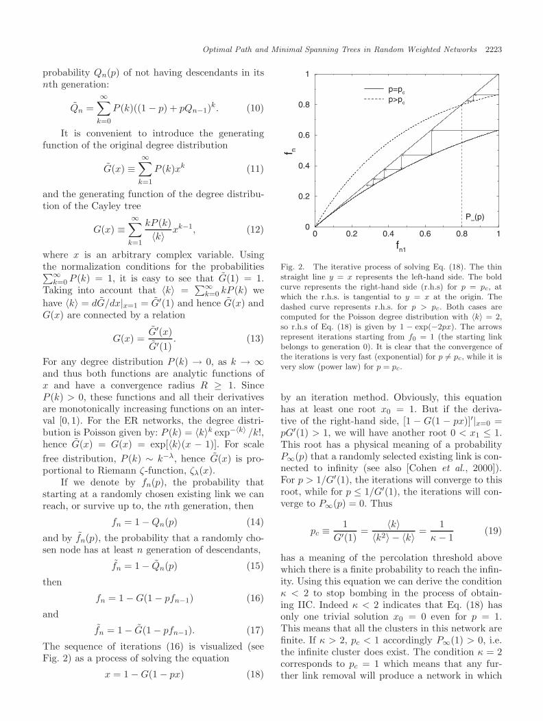
The sequence of iterations (16) is visualized (seeFig. 2) as a process of solving the equation
x = 1 − G(1 − px) (18)
0 0.2 0.4 0.6 0.8 1
fn1
0
0.2
0.4
0.6
0.8
1
f n
p=pc
p>pc
P∞(p)
Fig. 2. The iterative process of solving Eq. (18). The thinstraight line y = x represents the left-hand side. The boldcurve represents the right-hand side (r.h.s) for p = pc, atwhich the r.h.s. is tangential to y = x at the origin. Thedashed curve represents r.h.s. for p > pc. Both cases arecomputed for the Poisson degree distribution with 〈k〉 = 2,so r.h.s of Eq. (18) is given by 1 − exp(−2px). The arrowsrepresent iterations starting from f0 = 1 (the starting linkbelongs to generation 0). It is clear that the convergence ofthe iterations is very fast (exponential) for p �= pc, while it isvery slow (power law) for p = pc.
by an iteration method. Obviously, this equationhas at least one root x0 = 1. But if the deriva-tive of the right-hand side, [1 − G(1 − px)]′|x=0 =pG′(1) > 1, we will have another root 0 < x1 ≤ 1.This root has a physical meaning of a probabilityP∞(p) that a randomly selected existing link is con-nected to infinity (see also [Cohen et al., 2000]).For p > 1/G′(1), the iterations will converge to thisroot, while for p ≤ 1/G′(1), the iterations will con-verge to P∞(p) = 0. Thus
pc ≡ 1G′(1)
=〈k〉
〈k2〉 − 〈k〉 =1
κ − 1(19)
has a meaning of the percolation threshold abovewhich there is a finite probability to reach the infin-ity. Using this equation we can derive the conditionκ < 2 to stop bombing in the process of obtain-ing IIC. Indeed κ < 2 indicates that Eq. (18) hasonly one trivial solution x0 = 0 even for p = 1.This means that all the clusters in this network arefinite. If κ > 2, pc < 1 accordingly P∞(1) > 0, i.e.the infinite cluster does exist. The condition κ = 2corresponds to pc = 1 which means that any fur-ther link removal will produce a network in which
2224 L. A. Braunstein et al.
P∞(1) = 0, i.e. the network with only finite clusters,while at p = 1, the infinite cluster is incipient.
The probability that a randomly chosen nodeis connected to infinity can be determined as
P∞(p) = 1 − G(1 − pP∞(p)), (20)
where P∞(p) is a nontrivial solution of Eq. (18). Forsome degree distributions including Poisson distri-bution, P∞(1) < 1. This indicates that a randomlychosen node on the original network may not belongto the giant component of the network. In fact, theoptimal path between nodes A and B exists if bothbelong to the giant component. Provided that A andB both belong to the giant component, the proba-bility that they are still connected when the fraction1 − p of bonds is removed is
Π(p) =
(P∞(p)P∞(1)
)2
. (21)
Translating this condition to the bombing algorithmof generating an optimal path, Π(p) is the proba-bility that the maximum random number along theoptimal path rmax ≤ p. Indeed, Π(p) is the proba-bility that when only a fraction p of links remains,the connectivity between A and B still exists. Hencermax ≤ p. Thus, Π(rmax) is the cumulative distribu-tion of rmax. The probability density of rmax is thusequal to the derivative of Π(p) with respect to p:
P (rmax) =d
dpΠ(p)
∣∣∣p=rmax
. (22)
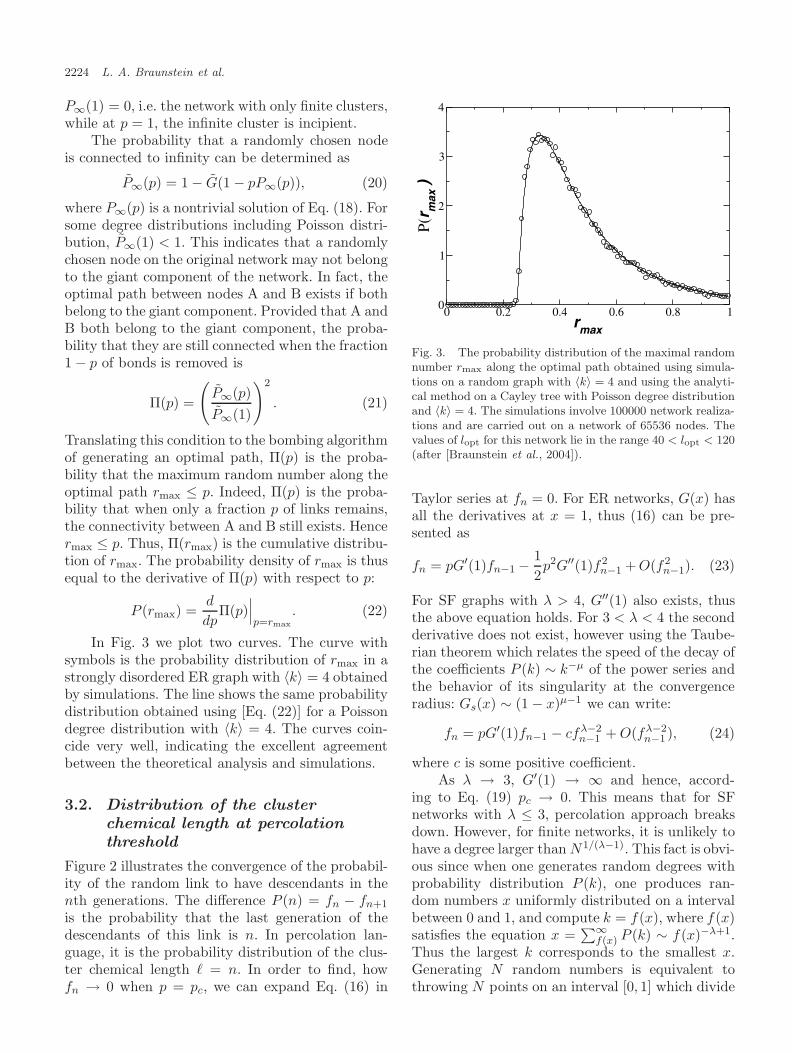
In Fig. 3 we plot two curves. The curve withsymbols is the probability distribution of rmax in astrongly disordered ER graph with 〈k〉 = 4 obtainedby simulations. The line shows the same probabilitydistribution obtained using [Eq. (22)] for a Poissondegree distribution with 〈k〉 = 4. The curves coin-cide very well, indicating the excellent agreementbetween the theoretical analysis and simulations.
3.2. Distribution of the clusterchemical length at percolationthreshold
Figure 2 illustrates the convergence of the probabil-ity of the random link to have descendants in thenth generations. The difference P (n) = fn − fn+1
is the probability that the last generation of thedescendants of this link is n. In percolation lan-guage, it is the probability distribution of the clus-ter chemical length � = n. In order to find, howfn → 0 when p = pc, we can expand Eq. (16) in
0 0.2 0.4 0.6 0.8 1rmax
0
1
2
3
4
P(r m
ax)
Fig. 3. The probability distribution of the maximal randomnumber rmax along the optimal path obtained using simula-tions on a random graph with 〈k〉 = 4 and using the analyti-cal method on a Cayley tree with Poisson degree distributionand 〈k〉 = 4. The simulations involve 100000 network realiza-tions and are carried out on a network of 65536 nodes. Thevalues of lopt for this network lie in the range 40 < lopt < 120(after [Braunstein et al., 2004]).
Taylor series at fn = 0. For ER networks, G(x) hasall the derivatives at x = 1, thus (16) can be pre-sented as
fn = pG′(1)fn−1 − 12p2G′′(1)f2
n−1 + O(f2n−1). (23)
For SF graphs with λ > 4, G′′(1) also exists, thusthe above equation holds. For 3 < λ < 4 the secondderivative does not exist, however using the Taube-rian theorem which relates the speed of the decay ofthe coefficients P (k) ∼ k−µ of the power series andthe behavior of its singularity at the convergenceradius: Gs(x) ∼ (1 − x)µ−1 we can write:
fn = pG′(1)fn−1 − cfλ−2n−1 + O(fλ−2
n−1 ), (24)
where c is some positive coefficient.As λ → 3, G′(1) → ∞ and hence, accord-
ing to Eq. (19) pc → 0. This means that for SFnetworks with λ ≤ 3, percolation approach breaksdown. However, for finite networks, it is unlikely tohave a degree larger than N1/(λ−1). This fact is obvi-ous since when one generates random degrees withprobability distribution P (k), one produces ran-dom numbers x uniformly distributed on a intervalbetween 0 and 1, and compute k = f(x), where f(x)satisfies the equation x =
∑∞f(x) P (k) ∼ f(x)−λ+1.
Thus the largest k corresponds to the smallest x.Generating N random numbers is equivalent tothrowing N points on an interval [0, 1] which divide
Optimal Path and Minimal Spanning Trees in Random Weighted Networks 2225
this interval into N + 1 segments whose lengths areidentically distributed with an exponential distri-bution. Thus the average value of the smallest x isequal to 1/(N + 1). Accordingly, the average valueof the largest k can be approximated as kmax =f(1/(N + 1)) ∼ N1/(λ−1) [Cohen et al., 2000]. Thusreplacing summation by integration up to kmax inthe expression for G′(1) ≈ ∫ kmax k−λ+2dk ∼ k3−λ
max =N (3−λ)/(λ−1). Hence for 2 < λ < 3 [Cohen et al.,2000].
pc ∼ N (λ−3)/(λ−1). (25)
When p < pc, fn ∼ (p/pc)n, i.e. the conver-gence is exponential. When p = pc, we will seek thesolution of the above recursion relations in a powerlaw form: fn ∼ n−θ. Expanding them in powersof n−1, and equating the leading powers, we haveθ + 1 = θ(λ − 2), from which we obtain
fn ∼ n−1/(λ−3), (26)
or
P (�) = f� − f�+1 ∼ �−τ� , (27)
where [Cohen et al., 2002; Cohen et al., 2002]
τ� =
2, λ > 4 ER
1(λ − 3)
+ 1, 3 < λ ≤ 4. (28)
The probability that a randomly selected node hasexactly � generations of descendants is equal to
P (�) = f� − f�+1 = G(1 − pf�) − G(1 − pf�−1)
∼ 〈k〉p(f� − f�−1). (29)
Thus it is characterized by the same τ� as P (�).Taylor expansions (23) and (24) can be used
to derive the behavior of P∞(p) as p → pc by let-ting fn = fn−1 = P∞(p) and solving the resultingequations with a leading term accuracy:
P∞(p) = (p − pc)β , (30)
where [Cohen et al., 2000]
β ={
1, λ > 4 ERλ − 3, 3 < λ ≤ 4
. (31)
3.3. Distribution of the clustersizes at percolation threshold
Using the generating functions [Cohen et al., 2002;Cohen et al., 2002; Callaway et al., 2000], one canalso find the distribution of the clusters sizes, P (s),
connected to a randomly selected link. For simplic-ity, let us again consider a link (conducting withprobability p) leading to a node of a degree k = 3,so it has only two outgoing links. The probabilitythat this link is connected to a cluster consisting ofs nodes obeys the following relations
P (s) = p∑
k+l=s−1
P (k)P (l) (32)
for s > 0 and P (0) = 1−p. Introducing the generat-ing function of the cluster size distribution H(x) =∑∞
0 P (s)xs, we have: H(x) = 1 − p + xpH2(x). Ina general Cayley tree with an arbitrary degree dis-tribution we have:
H(x) = 1 − p + xpG(H(x)). (33)
This equation defines the behavior of H(x) for x →1, and thus via the Tauberian theorem defines theasymptotic behavior of its coefficients P (s). Notethat H(1) is the cumulative probability of all finiteclusters. Thus (1−H(1)) = pP∞(p) is the probabil-ity that a randomly selected link conducting withprobability p is connected to infinity and Eq. (33)becomes equivalent to Eq. (18) for P∞(p).
Introducing δx = 1 − x and δH = 1 − H(x)and expanding G(x) around x = 1 at percola-tion threshold p = 1/G′(1), we have δHδx + pδx =cxδλ−2
H +O(δλ−2H ) which yields δH ∼ δ
1/(λ−2)x . Using
the Tauberian theorem we conclude [Cohen et al.,2002; Cohen et al., 2002]:
P (s) ∼ s−τs , (34)
where
τs =
32, λ > 4 ER
1λ − 2
+ 1, 3 < λ ≤ 4. (35)
Analogous considerations suggest that the probabil-ities P (s) that a randomly selected node belongs tothe cluster of size s produce the generating functionH(x) = G(H(x)). Since for λ > 3, G′′(1) < ∞, thesingularity of H(x) for x → 1 is of the same orderas the singularity of H(x) and thus its coefficients,P (s), also decay as s−τs .
Following [Stauffer & Aharony, 1994], we willshow that the distribution of all the disconnectedclusters in a network scales as Pall(s) = P (s)/s ∼s−τs+1. Indeed, let us select a random node inthis network. The number of nodes belonging to
2226 L. A. Braunstein et al.
the clusters of size s is NsPall(s)/∑∞
1 sPall(s) =NsPall(s)/〈s〉. Thus, P (s) = sPall(s)/〈s〉.
If we have a network of N nodes, the size ofthe largest cluster S is determined by the relation∑∞
s=S Pall(s) ∼ 1/N , which becomes clear if wedescribe a concrete realization of the cluster sizesby throwing N/〈s〉 random points representing clus-ters under the curve Pall(s). The average area corre-sponding to each of these points is 1/N and the areacorresponding to the rightmost point representingthe largest cluster is
∑∞s=S Pall(s) ∼ S−τs . Thus the
largest cluster (which coincides with IIC) in the net-work of N nodes scales as
S ∼ N1/τs . (36)
For ER graphs, the relation S ∼ N2/3 has beenderived in a classical work [Erdos & Renyi, 1959].
4. Scaling of the Length of theOptimal Path in Strong Disorder
The relations obtained in the previous subsectionsallow us to determine the scaling of the average opti-mal path length in a network of N nodes. Duringbombing, when we reach percolation threshold, wehave targeted only a tiny fraction of links (or nodes)on the optimal path, with rmax > pc which we haveto restore, because their removal would destroy theconnectivity. The majority of the links on the opti-mal path remains intact. All of them belong to theremaining percolation clusters which at percolationthreshold has a tree-like structure with no loops.At this point, the optimal path coincides with theshortest path, which is uniquely determined. Wewill describe this situation in detail in Sec. 6. Withhigh probability, the optimal path between any twonodes A and B goes through the largest clusterat the percolation threshold. Thus its length mustscale as the chemical length of the largest perco-lation cluster [Braunstein et al., 2003]. Assuminga power law relation between the cluster size s andits chemical dimension �, s = �d� , and using the factthat both of the quantities have power law distribu-tions P (�)d� = P (s)ds, we have �−τ� = �−d�τs+d�−1.Thus [Barrat et al., 2004]
d� =τl − 1τs − 1
. (37)
Therefore, S ∼ �d�opt and using (36) we have �opt ∼
S1/d� ∼ Nνopt , where
νopt =1
d�τs. (38)
Using Eqs. (35) and (28) for τs and τ� respectively,we have
νopt =
13, λ > 4, ER
λ − 3λ − 1
, 3 < λ ≤ 4
. (39)
Note that λ = 4 corresponds to the special casewhen G′′(1) diverges, in this case the Tauberian the-orem predicts logarithmic corrections, and hence weexpect �opt ∼ N1/3/ln N for λ = 4.
We review above the exact results for the Cay-ley tree, from which using heuristic arguments wehave derived the scaling relation between the aver-age length of the optimal path and the numberof nodes in the network. Now we will show howthe same predictions can be obtained using generalpercolation theory. We will also present numericaldata supporting our heuristic arguments. We beginby considering the ER graph. At criticality, it isequivalent to percolation on the Cayley tree or per-colation at the upper critical dimension dc = 6. Forthe ER graph, we derived above that the mass ofthe IIC, S, scales as N2/3 [Erdos & Renyi, 1959].This result can also be obtained in the frameworkof percolation theory for dc = 6. Since S ∼ Rdf andN ∼ Rd (where df is the fractal dimension and Rthe spatial diameter of the cluster), it follows thatS ∼ Ndf /d and for dc = 6, df = 4 [Bunde & Havlin,1996] we obtain S ∼ N2/3 [Watts, 2003].
It is also known [Bunde & Havlin, 1996] that,at criticality, at the upper critical dimension, theaverage shortest path length �min ∼ R2, like arandom walk and therefore S ∼ �d�
min with d� = 2.Thus
�min ∼ �opt ∼ S1/d� ∼ N2/3d� ∼ Nνopt , (40)
where νopt = 2/3d� = 1/3.For SF networks, we can also use the percola-
tion results at criticality. It was found [Cohen et al.,2002; Cohen et al., 2002] (see Sec. 3) that d� = 2 forλ > 4, d� = (λ−2)/(λ−3) for 3 < λ < 4, S ∼ N2/3
for λ > 4, and S ∼ N (λ−2)/(λ−1) for 3 < λ ≤ 4.Hence, we conclude that
�min ∼ �opt ∼{
N1/3 λ > 4
N (λ−3)/(λ−1) 3 < λ ≤ 4. (41)
Thus νopt = 1/3 for ER and SF with λ > 4, andνopt = (λ− 3)/(λ − 1) for SF with 3 < λ < 4. Sincefor SF networks with λ > 4 the scaling behavior of�opt is the same as for ER graphs and for λ < 4 the
Optimal Path and Minimal Spanning Trees in Random Weighted Networks 2227
scaling is different, we can regard SF networks as ageneralization of ER graphs.
Next, we describe the details of the numer-ical simulations and show that the results agreewith the above theoretical predictions. We performnumerical simulations in the strong disorder limitby the method described in Sec. 2.4 for ER and SFnetworks. We also perform additional simulations
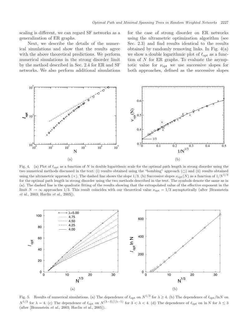
for the case of strong disorder on ER networksusing the ultrametric optimization algorithm (seeSec. 2.3) and find results identical to the resultsobtained by randomly removing links. In Fig. 4(a)we show a double logarithmic plot of �opt as a func-tion of N for ER graphs. To evaluate the asymp-totic value for νopt we use successive slopes forboth approaches, defined as the successive slopes
100
101
102
103
104
105
N
100
101
102
l opt
0 0.1 0.2 0.3 0.4 0.5
1/N1/3
0.3
0.4
0.5
0.6
ν opt(N
)
1/3
(a) (b)
Fig. 4. (a) Plot of �opt as a function of N in double logarithmic scale for the optimal path length in strong disorder using thetwo numerical methods discussed in the text: (i) results obtained using the “bombing” approach (©) and (ii) results obtained
using the ultrametric approach (×). The dashed line shows the slope 1/3. (b) Successive slopes νopt(N) as a function of 1/N1/3
for the optimal path length in strong disorder using the two methods described in the text. The symbols denote the same as in(a). The dashed line is the quadratic fitting of the results showing that the extrapolated value of the effective exponent in thelimit N → ∞ approaches 1/3. This result coincides with our theoretical value νopt = 1/3 asymptotically (after [Braunsteinet al., 2003; Havlin et al., 2005]).
0 10 20 30
N1/3
0
20
40
60
80
100
l opt
λ=5.004.754.504.254.00
0 10 20 30
N1/3
0
200
400
600
l optln
N
(a) (b)
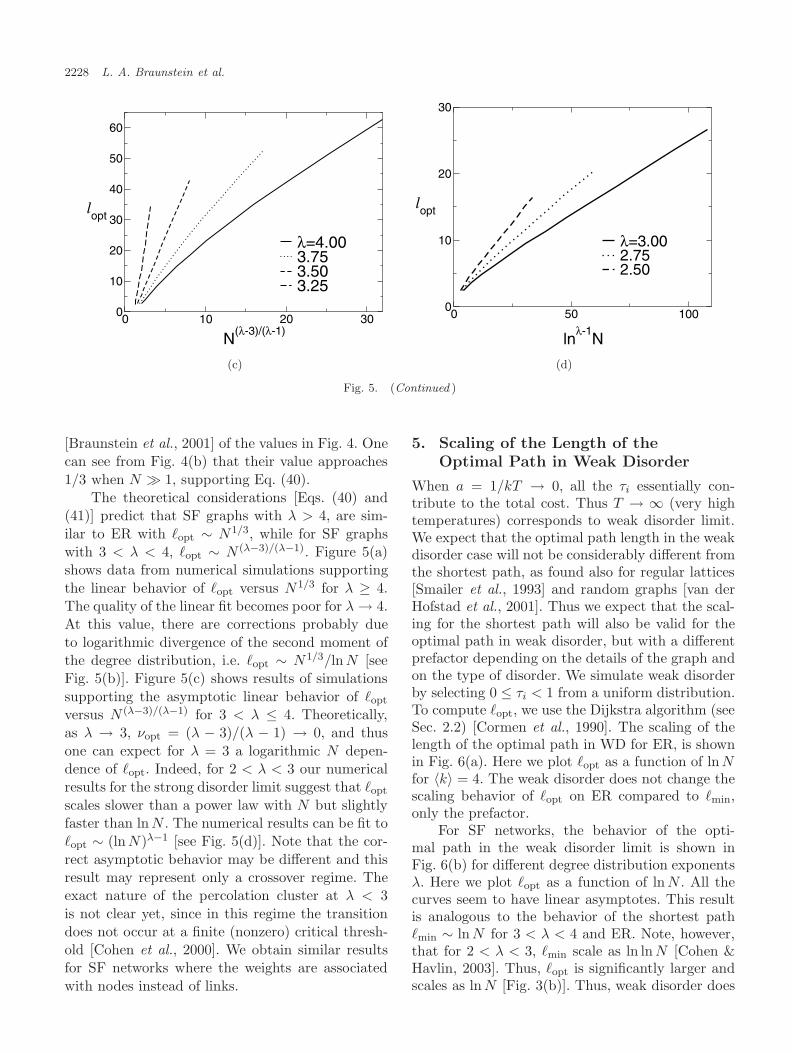
Fig. 5. Results of numerical simulations. (a) The dependence of �opt on N1/3 for λ ≥ 4. (b) The dependence of �opt/lnN on
N1/3 for λ = 4. (c) The dependence of �opt on N(λ−3)/(λ−1) for 3 < λ < 4. (d) The dependence of �opt on ln N for λ ≤ 3(after [Braunstein et al., 2003; Havlin et al., 2005]).
2228 L. A. Braunstein et al.
0 10 20 30
N(λ-3)/(λ-1)
0
10
20
30
40
50
60
lopt
λ=4.003.753.503.25
0 50 100
lnλ-1
N
0
10
20
30
lopt
λ=3.002.752.50
(c) (d)
Fig. 5. (Continued )
[Braunstein et al., 2001] of the values in Fig. 4. Onecan see from Fig. 4(b) that their value approaches1/3 when N � 1, supporting Eq. (40).
The theoretical considerations [Eqs. (40) and(41)] predict that SF graphs with λ > 4, are sim-ilar to ER with �opt ∼ N1/3, while for SF graphswith 3 < λ < 4, �opt ∼ N (λ−3)/(λ−1). Figure 5(a)shows data from numerical simulations supportingthe linear behavior of �opt versus N1/3 for λ ≥ 4.The quality of the linear fit becomes poor for λ → 4.At this value, there are corrections probably dueto logarithmic divergence of the second moment ofthe degree distribution, i.e. �opt ∼ N1/3/ln N [seeFig. 5(b)]. Figure 5(c) shows results of simulationssupporting the asymptotic linear behavior of �opt
versus N (λ−3)/(λ−1) for 3 < λ ≤ 4. Theoretically,as λ → 3, νopt = (λ − 3)/(λ − 1) → 0, and thusone can expect for λ = 3 a logarithmic N depen-dence of �opt. Indeed, for 2 < λ < 3 our numericalresults for the strong disorder limit suggest that �opt
scales slower than a power law with N but slightlyfaster than ln N . The numerical results can be fit to�opt ∼ (ln N)λ−1 [see Fig. 5(d)]. Note that the cor-rect asymptotic behavior may be different and thisresult may represent only a crossover regime. Theexact nature of the percolation cluster at λ < 3is not clear yet, since in this regime the transitiondoes not occur at a finite (nonzero) critical thresh-old [Cohen et al., 2000]. We obtain similar resultsfor SF networks where the weights are associatedwith nodes instead of links.
5. Scaling of the Length of theOptimal Path in Weak Disorder
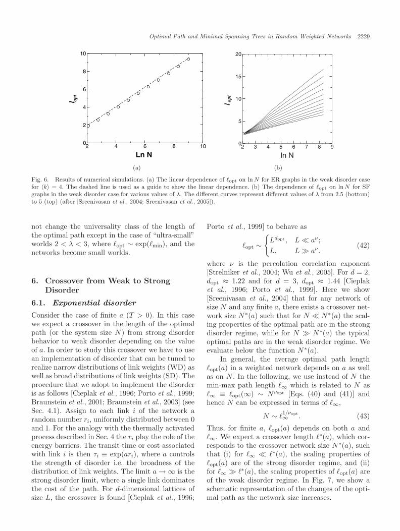
When a = 1/kT → 0, all the τi essentially con-tribute to the total cost. Thus T → ∞ (very hightemperatures) corresponds to weak disorder limit.We expect that the optimal path length in the weakdisorder case will not be considerably different fromthe shortest path, as found also for regular lattices[Smailer et al., 1993] and random graphs [van derHofstad et al., 2001]. Thus we expect that the scal-ing for the shortest path will also be valid for theoptimal path in weak disorder, but with a differentprefactor depending on the details of the graph andon the type of disorder. We simulate weak disorderby selecting 0 ≤ τi < 1 from a uniform distribution.To compute �opt, we use the Dijkstra algorithm (seeSec. 2.2) [Cormen et al., 1990]. The scaling of thelength of the optimal path in WD for ER, is shownin Fig. 6(a). Here we plot �opt as a function of lnNfor 〈k〉 = 4. The weak disorder does not change thescaling behavior of �opt on ER compared to �min,only the prefactor.
For SF networks, the behavior of the opti-mal path in the weak disorder limit is shown inFig. 6(b) for different degree distribution exponentsλ. Here we plot �opt as a function of ln N . All thecurves seem to have linear asymptotes. This resultis analogous to the behavior of the shortest path�min ∼ ln N for 3 < λ < 4 and ER. Note, however,that for 2 < λ < 3, �min scale as ln ln N [Cohen &Havlin, 2003]. Thus, �opt is significantly larger andscales as ln N [Fig. 3(b)]. Thus, weak disorder does
Optimal Path and Minimal Spanning Trees in Random Weighted Networks 2229
2 4 6 8 10
Ln N
0
2
4
6
8
10
l opt
2 3 4 5 6 7 8 9
ln N
0
5
10
15
20
l opt
(a) (b)
Fig. 6. Results of numerical simulations. (a) The linear dependence of �opt on ln N for ER graphs in the weak disorder casefor 〈k〉 = 4. The dashed line is used as a guide to show the linear dependence. (b) The dependence of �opt on ln N for SFgraphs in the weak disorder case for various values of λ. The different curves represent different values of λ from 2.5 (bottom)to 5 (top) (after [Sreenivasan et al., 2004; Sreenivasan et al., 2005]).
not change the universality class of the length ofthe optimal path except in the case of “ultra-small”worlds 2 < λ < 3, where �opt ∼ exp(�min), and thenetworks become small worlds.
6. Crossover from Weak to StrongDisorder
6.1. Exponential disorder
Consider the case of finite a (T > 0). In this casewe expect a crossover in the length of the optimalpath (or the system size N) from strong disorderbehavior to weak disorder depending on the valueof a. In order to study this crossover we have to usean implementation of disorder that can be tuned torealize narrow distributions of link weights (WD) aswell as broad distributions of link weights (SD). Theprocedure that we adopt to implement the disorderis as follows [Cieplak et al., 1996; Porto et al., 1999;Braunstein et al., 2001; Braunstein et al., 2003] (seeSec. 4.1). Assign to each link i of the network arandom number ri, uniformly distributed between 0and 1. For the analogy with the thermally activatedprocess described in Sec. 4 the ri play the role of theenergy barriers. The transit time or cost associatedwith link i is then τi ≡ exp(ari), where a controlsthe strength of disorder i.e. the broadness of thedistribution of link weights. The limit a → ∞ is thestrong disorder limit, where a single link dominatesthe cost of the path. For d-dimensional lattices ofsize L, the crossover is found [Cieplak et al., 1996;
Porto et al., 1999] to behave as
�opt ∼{
Ldopt , L � aν ;L, L � aν .
(42)
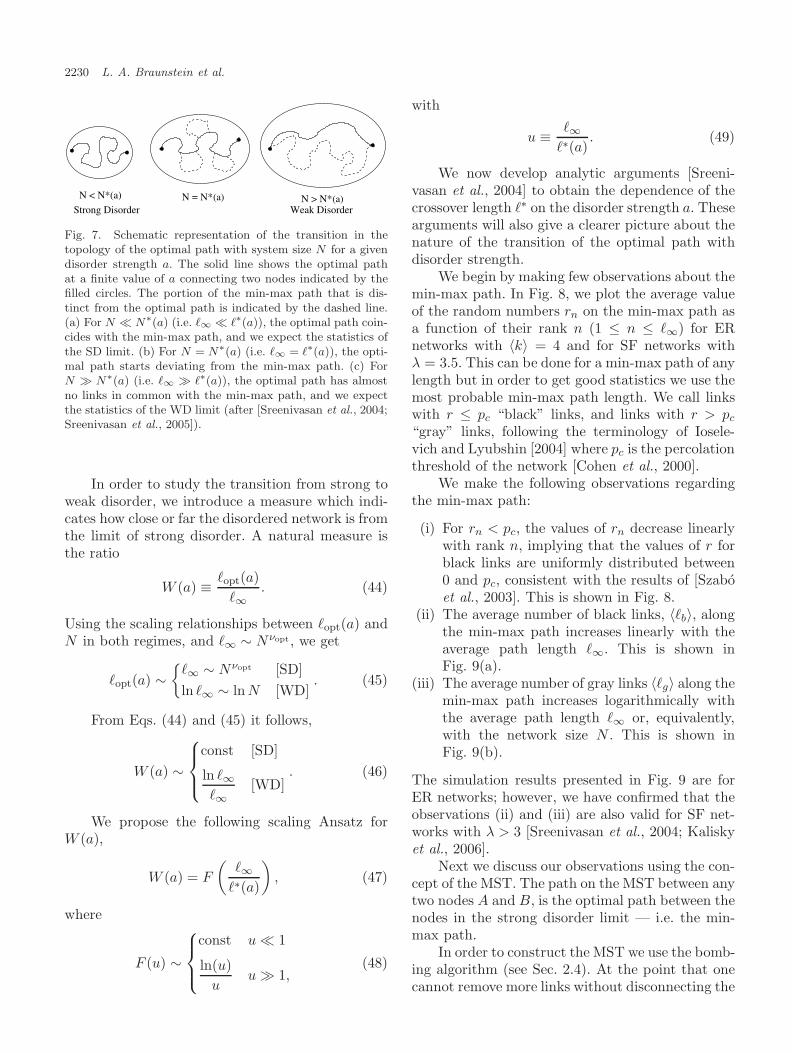
where ν is the percolation correlation exponent[Strelniker et al., 2004; Wu et al., 2005]. For d = 2,dopt ≈ 1.22 and for d = 3, dopt ≈ 1.44 [Cieplaket al., 1996; Porto et al., 1999]. Here we show[Sreenivasan et al., 2004] that for any network ofsize N and any finite a, there exists a crossover net-work size N∗(a) such that for N � N∗(a) the scal-ing properties of the optimal path are in the strongdisorder regime, while for N � N∗(a) the typicaloptimal paths are in the weak disorder regime. Weevaluate below the function N∗(a).
In general, the average optimal path length�opt(a) in a weighted network depends on a as wellas on N . In the following, we use instead of N themin-max path length �∞ which is related to N as�∞ ≡ �opt(∞) ∼ Nνopt [Eqs. (40) and (41)] andhence N can be expressed in terms of �∞,
N ∼ �1/νopt∞ . (43)
Thus, for finite a, �opt(a) depends on both a and�∞. We expect a crossover length �∗(a), which cor-responds to the crossover network size N∗(a), suchthat (i) for �∞ � �∗(a), the scaling properties of�opt(a) are of the strong disorder regime, and (ii)for �∞ � �∗(a), the scaling properties of �opt(a) areof the weak disorder regime. In Fig. 7, we show aschematic representation of the changes of the opti-mal path as the network size increases.
2230 L. A. Braunstein et al.
Strong DisorderN = N* N > N*
Weak Disorder
N < N*(a) (a) (a)
Fig. 7. Schematic representation of the transition in thetopology of the optimal path with system size N for a givendisorder strength a. The solid line shows the optimal pathat a finite value of a connecting two nodes indicated by thefilled circles. The portion of the min-max path that is dis-tinct from the optimal path is indicated by the dashed line.(a) For N � N∗(a) (i.e. �∞ � �∗(a)), the optimal path coin-cides with the min-max path, and we expect the statistics ofthe SD limit. (b) For N = N∗(a) (i.e. �∞ = �∗(a)), the opti-mal path starts deviating from the min-max path. (c) ForN � N∗(a) (i.e. �∞ � �∗(a)), the optimal path has almostno links in common with the min-max path, and we expectthe statistics of the WD limit (after [Sreenivasan et al., 2004;Sreenivasan et al., 2005]).
In order to study the transition from strong toweak disorder, we introduce a measure which indi-cates how close or far the disordered network is fromthe limit of strong disorder. A natural measure isthe ratio
W (a) ≡ �opt(a)�∞
. (44)
Using the scaling relationships between �opt(a) andN in both regimes, and �∞ ∼ Nνopt , we get
�opt(a) ∼{
�∞ ∼ Nνopt [SD]ln �∞ ∼ ln N [WD]
. (45)
From Eqs. (44) and (45) it follows,
W (a) ∼
const [SD]
ln �∞�∞
[WD]. (46)
We propose the following scaling Ansatz forW (a),
W (a) = F
(�∞
�∗(a)
), (47)
where
F (u) ∼
const u � 1
ln(u)u
u � 1,(48)
with
u ≡ �∞�∗(a)
. (49)
We now develop analytic arguments [Sreeni-vasan et al., 2004] to obtain the dependence of thecrossover length �∗ on the disorder strength a. Thesearguments will also give a clearer picture about thenature of the transition of the optimal path withdisorder strength.
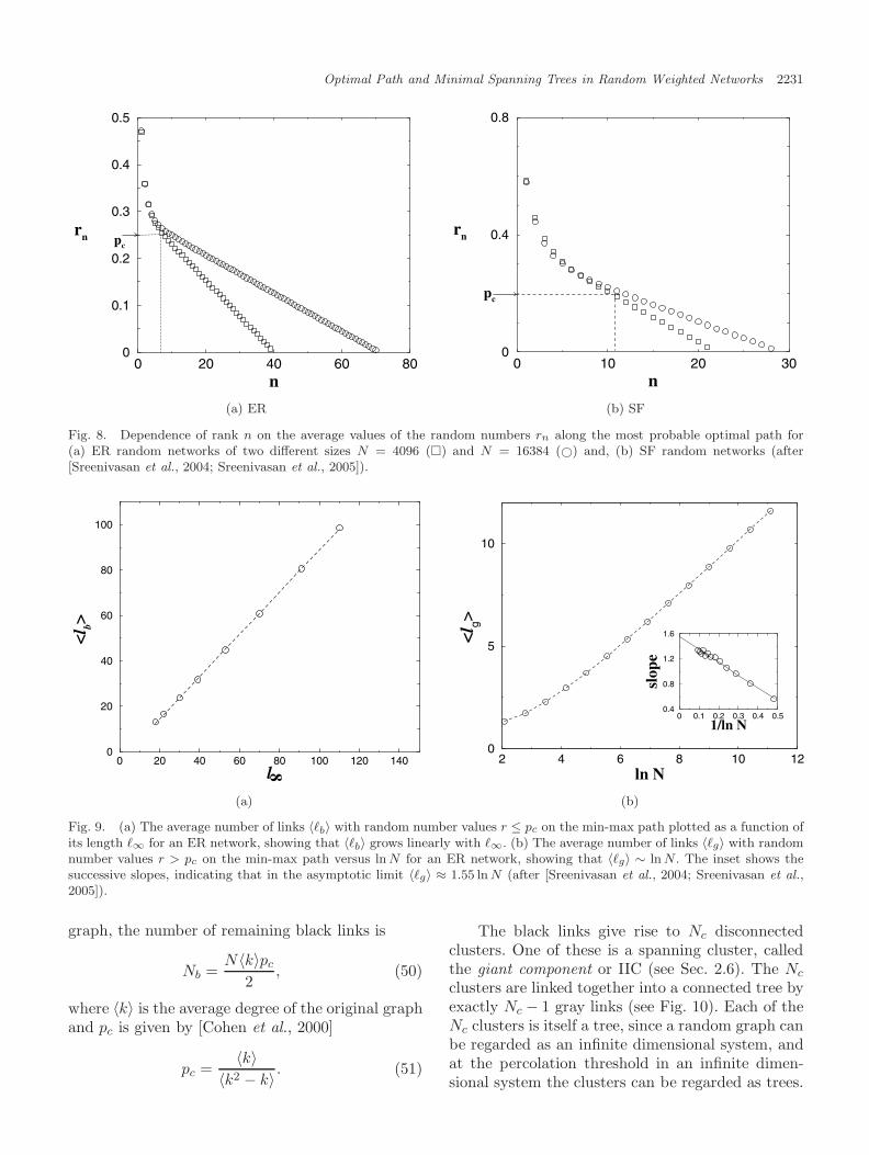
We begin by making few observations about themin-max path. In Fig. 8, we plot the average valueof the random numbers rn on the min-max path asa function of their rank n (1 ≤ n ≤ �∞) for ERnetworks with 〈k〉 = 4 and for SF networks withλ = 3.5. This can be done for a min-max path of anylength but in order to get good statistics we use themost probable min-max path length. We call linkswith r ≤ pc “black” links, and links with r > pc
“gray” links, following the terminology of Iosele-vich and Lyubshin [2004] where pc is the percolationthreshold of the network [Cohen et al., 2000].
We make the following observations regardingthe min-max path:
(i) For rn < pc, the values of rn decrease linearlywith rank n, implying that the values of r forblack links are uniformly distributed between0 and pc, consistent with the results of [Szaboet al., 2003]. This is shown in Fig. 8.
(ii) The average number of black links, 〈�b〉, alongthe min-max path increases linearly with theaverage path length �∞. This is shown inFig. 9(a).
(iii) The average number of gray links 〈�g〉 along themin-max path increases logarithmically withthe average path length �∞ or, equivalently,with the network size N . This is shown inFig. 9(b).
The simulation results presented in Fig. 9 are forER networks; however, we have confirmed that theobservations (ii) and (iii) are also valid for SF net-works with λ > 3 [Sreenivasan et al., 2004; Kaliskyet al., 2006].
Next we discuss our observations using the con-cept of the MST. The path on the MST between anytwo nodes A and B, is the optimal path between thenodes in the strong disorder limit — i.e. the min-max path.
In order to construct the MST we use the bomb-ing algorithm (see Sec. 2.4). At the point that onecannot remove more links without disconnecting the
Optimal Path and Minimal Spanning Trees in Random Weighted Networks 2231
0 20 40 60 80n
0
0.1
0.2
0.3
0.4
0.5
rn pc
0 10 20 30n
0
0.4
0.8
rn
pc
(a) ER (b) SF
Fig. 8. Dependence of rank n on the average values of the random numbers rn along the most probable optimal path for(a) ER random networks of two different sizes N = 4096 (�) and N = 16384 (©) and, (b) SF random networks (after[Sreenivasan et al., 2004; Sreenivasan et al., 2005]).
0 20 40 60 80 100 120 140l
0
20
40
60
80
100
<lb>
8
2 4 6 8 10 12ln N
0
5
10
<lg>
0 0.1 0.2 0.3 0.4 0.51/ln N
0.4
0.8
1.2
1.6
slop
e
(a) (b)
Fig. 9. (a) The average number of links 〈�b〉 with random number values r ≤ pc on the min-max path plotted as a function ofits length �∞ for an ER network, showing that 〈�b〉 grows linearly with �∞. (b) The average number of links 〈�g〉 with randomnumber values r > pc on the min-max path versus ln N for an ER network, showing that 〈�g〉 ∼ ln N . The inset shows thesuccessive slopes, indicating that in the asymptotic limit 〈�g〉 ≈ 1.55 ln N (after [Sreenivasan et al., 2004; Sreenivasan et al.,2005]).
graph, the number of remaining black links is
Nb =N〈k〉pc
2, (50)
where 〈k〉 is the average degree of the original graphand pc is given by [Cohen et al., 2000]
pc =〈k〉
〈k2 − k〉 . (51)
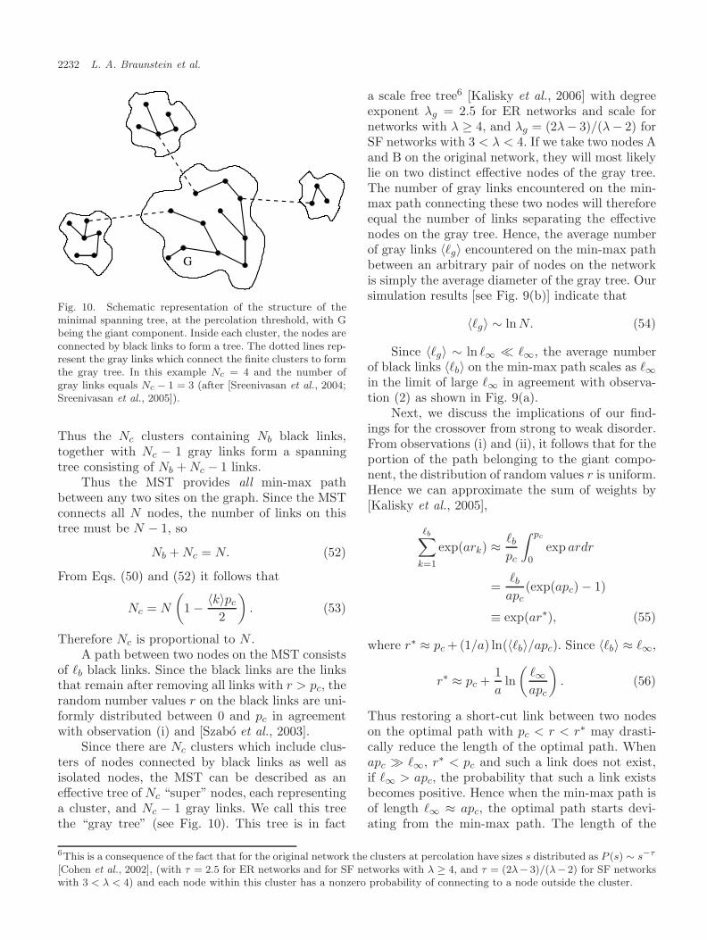
The black links give rise to Nc disconnectedclusters. One of these is a spanning cluster, calledthe giant component or IIC (see Sec. 2.6). The Nc
clusters are linked together into a connected tree byexactly Nc − 1 gray links (see Fig. 10). Each of theNc clusters is itself a tree, since a random graph canbe regarded as an infinite dimensional system, andat the percolation threshold in an infinite dimen-sional system the clusters can be regarded as trees.
2232 L. A. Braunstein et al.
G
Fig. 10. Schematic representation of the structure of theminimal spanning tree, at the percolation threshold, with Gbeing the giant component. Inside each cluster, the nodes areconnected by black links to form a tree. The dotted lines rep-resent the gray links which connect the finite clusters to formthe gray tree. In this example Nc = 4 and the number ofgray links equals Nc − 1 = 3 (after [Sreenivasan et al., 2004;Sreenivasan et al., 2005]).
Thus the Nc clusters containing Nb black links,together with Nc − 1 gray links form a spanningtree consisting of Nb + Nc − 1 links.
Thus the MST provides all min-max pathbetween any two sites on the graph. Since the MSTconnects all N nodes, the number of links on thistree must be N − 1, so
Nb + Nc = N. (52)
From Eqs. (50) and (52) it follows that
Nc = N
(1 − 〈k〉pc
2
). (53)
Therefore Nc is proportional to N .A path between two nodes on the MST consists
of �b black links. Since the black links are the linksthat remain after removing all links with r > pc, therandom number values r on the black links are uni-formly distributed between 0 and pc in agreementwith observation (i) and [Szabo et al., 2003].
Since there are Nc clusters which include clus-ters of nodes connected by black links as well asisolated nodes, the MST can be described as aneffective tree of Nc “super” nodes, each representinga cluster, and Nc − 1 gray links. We call this treethe “gray tree” (see Fig. 10). This tree is in fact
a scale free tree6 [Kalisky et al., 2006] with degreeexponent λg = 2.5 for ER networks and scale fornetworks with λ ≥ 4, and λg = (2λ− 3)/(λ− 2) forSF networks with 3 < λ < 4. If we take two nodes Aand B on the original network, they will most likelylie on two distinct effective nodes of the gray tree.The number of gray links encountered on the min-max path connecting these two nodes will thereforeequal the number of links separating the effectivenodes on the gray tree. Hence, the average numberof gray links 〈�g〉 encountered on the min-max pathbetween an arbitrary pair of nodes on the networkis simply the average diameter of the gray tree. Oursimulation results [see Fig. 9(b)] indicate that
〈�g〉 ∼ ln N. (54)
Since 〈�g〉 ∼ ln �∞ � �∞, the average numberof black links 〈�b〉 on the min-max path scales as �∞in the limit of large �∞ in agreement with observa-tion (2) as shown in Fig. 9(a).
Next, we discuss the implications of our find-ings for the crossover from strong to weak disorder.From observations (i) and (ii), it follows that for theportion of the path belonging to the giant compo-nent, the distribution of random values r is uniform.Hence we can approximate the sum of weights by[Kalisky et al., 2005],
�b∑k=1
exp(ark) ≈ �b
pc
∫ pc
0exp ardr
=�b
apc(exp(apc) − 1)
≡ exp(ar∗), (55)
where r∗ ≈ pc + (1/a) ln(〈�b〉/apc). Since 〈�b〉 ≈ �∞,
r∗ ≈ pc +1a
ln(
�∞apc
). (56)
Thus restoring a short-cut link between two nodeson the optimal path with pc < r < r∗ may drasti-cally reduce the length of the optimal path. Whenapc � �∞, r∗ < pc and such a link does not exist,if �∞ > apc, the probability that such a link existsbecomes positive. Hence when the min-max path isof length �∞ ≈ apc, the optimal path starts devi-ating from the min-max path. The length of the
6This is a consequence of the fact that for the original network the clusters at percolation have sizes s distributed as P (s) ∼ s−τ
[Cohen et al., 2002], (with τ = 2.5 for ER networks and for SF networks with λ ≥ 4, and τ = (2λ− 3)/(λ− 2) for SF networkswith 3 < λ < 4) and each node within this cluster has a nonzero probability of connecting to a node outside the cluster.
Optimal Path and Minimal Spanning Trees in Random Weighted Networks 2233
0 5 10 15l / a
0.2
0.4
0.6
0.8
1.0
W(a) 3 2 1 0ln (l /a)
0.8
0.9
1.0
W(a
)
8
8
0 1 2 3 4l / a
0.5
0.6
0.7
0.8
0.9
1.0
W(a) 4 3 2 1 0ln(l / a)
0.85
0.90
0.95
1.00
W(a
)
8
8
(a) ER (b) SF
Fig. 11. Test of Eqs. (47) and (48). (a) W (a) plotted as a function of �∞/a for different values of a for ER networks with〈k〉 = 4. The different symbols represent different a values: a = 8(©), a = 16(�), a = 22(�), a = 32(�), a = 45(+) anda = 64(∗). (b) Same as SF networks with λ = 3.5. The symbols correspond to the same values of disorder as in (a). The insetsshow W (a) plotted against log(l∞/a), and indicate for �∞ � a, W (a) approaches a constant in agreement with Eq. (48) (after[Sreenivasan et al., 2004; Sreenivasan et al., 2005]).
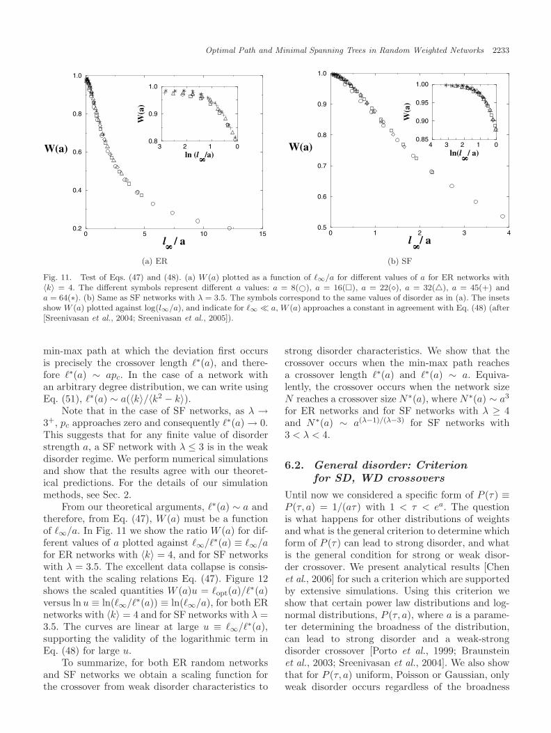
min-max path at which the deviation first occursis precisely the crossover length �∗(a), and there-fore �∗(a) ∼ apc. In the case of a network withan arbitrary degree distribution, we can write usingEq. (51), �∗(a) ∼ a(〈k〉/〈k2 − k〉).
Note that in the case of SF networks, as λ →3+, pc approaches zero and consequently �∗(a) → 0.This suggests that for any finite value of disorderstrength a, a SF network with λ ≤ 3 is in the weakdisorder regime. We perform numerical simulationsand show that the results agree with our theoret-ical predictions. For the details of our simulationmethods, see Sec. 2.
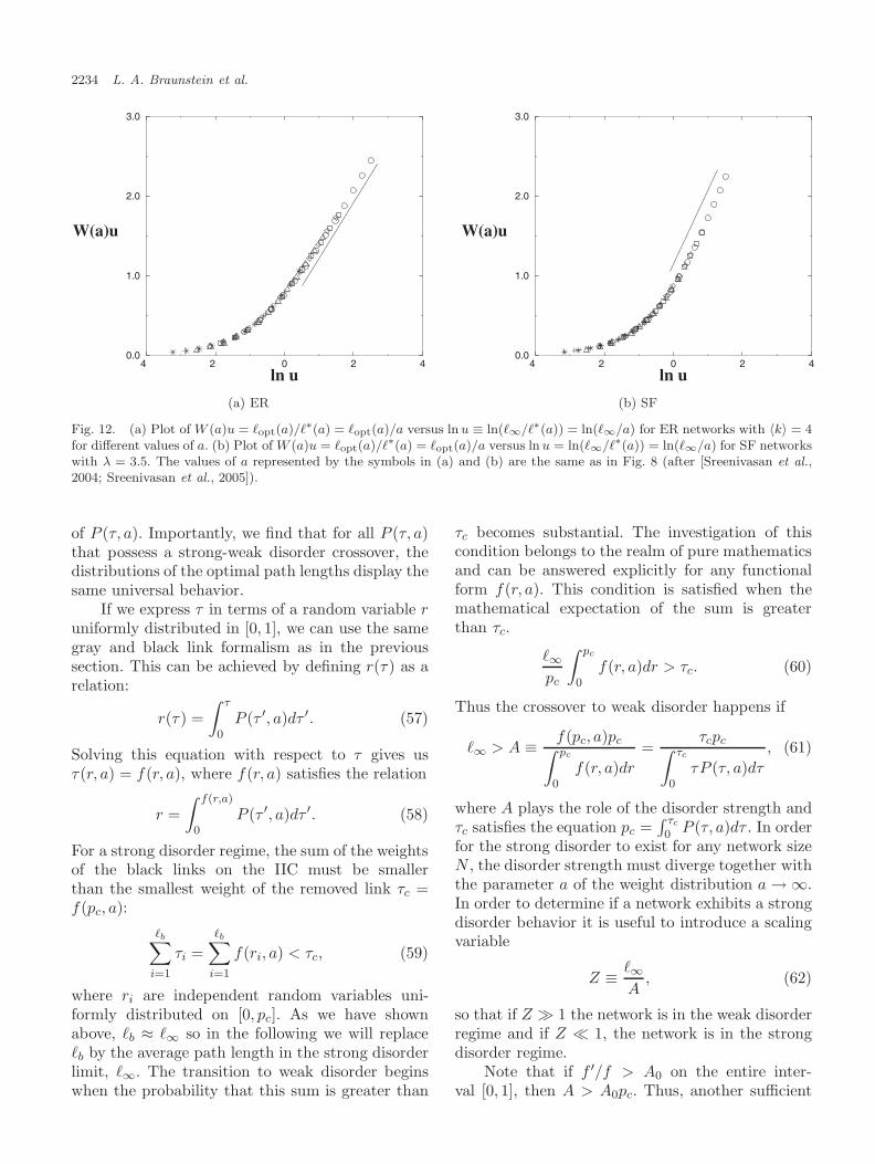
From our theoretical arguments, �∗(a) ∼ a andtherefore, from Eq. (47), W (a) must be a functionof �∞/a. In Fig. 11 we show the ratio W (a) for dif-ferent values of a plotted against �∞/�∗(a) ≡ �∞/afor ER networks with 〈k〉 = 4, and for SF networkswith λ = 3.5. The excellent data collapse is consis-tent with the scaling relations Eq. (47). Figure 12shows the scaled quantities W (a)u = �opt(a)/�∗(a)versus ln u ≡ ln(�∞/�∗(a)) ≡ ln(�∞/a), for both ERnetworks with 〈k〉 = 4 and for SF networks with λ =3.5. The curves are linear at large u ≡ �∞/�∗(a),supporting the validity of the logarithmic term inEq. (48) for large u.
To summarize, for both ER random networksand SF networks we obtain a scaling function forthe crossover from weak disorder characteristics to
strong disorder characteristics. We show that thecrossover occurs when the min-max path reachesa crossover length �∗(a) and �∗(a) ∼ a. Equiva-lently, the crossover occurs when the network sizeN reaches a crossover size N∗(a), where N∗(a) ∼ a3
for ER networks and for SF networks with λ ≥ 4and N∗(a) ∼ a(λ−1)/(λ−3) for SF networks with3 < λ < 4.
6.2. General disorder: Criterionfor SD, WD crossovers
Until now we considered a specific form of P (τ) ≡P (τ, a) = 1/(aτ) with 1 < τ < ea. The questionis what happens for other distributions of weightsand what is the general criterion to determine whichform of P (τ) can lead to strong disorder, and whatis the general condition for strong or weak disor-der crossover. We present analytical results [Chenet al., 2006] for such a criterion which are supportedby extensive simulations. Using this criterion weshow that certain power law distributions and log-normal distributions, P (τ, a), where a is a parame-ter determining the broadness of the distribution,can lead to strong disorder and a weak-strongdisorder crossover [Porto et al., 1999; Braunsteinet al., 2003; Sreenivasan et al., 2004]. We also showthat for P (τ, a) uniform, Poisson or Gaussian, onlyweak disorder occurs regardless of the broadness
2234 L. A. Braunstein et al.
4 2 0 2 4ln u
0.0
1.0
2.0
3.0
W(a)u
4 2 0 2 4ln u
0.0
1.0
2.0
3.0
W(a)u
(a) ER (b) SF
Fig. 12. (a) Plot of W (a)u = �opt(a)/�∗(a) = �opt(a)/a versus ln u ≡ ln(�∞/�∗(a)) = ln(�∞/a) for ER networks with 〈k〉 = 4for different values of a. (b) Plot of W (a)u = �opt(a)/�∗(a) = �opt(a)/a versus ln u = ln(�∞/�∗(a)) = ln(�∞/a) for SF networkswith λ = 3.5. The values of a represented by the symbols in (a) and (b) are the same as in Fig. 8 (after [Sreenivasan et al.,2004; Sreenivasan et al., 2005]).
of P (τ, a). Importantly, we find that for all P (τ, a)that possess a strong-weak disorder crossover, thedistributions of the optimal path lengths display thesame universal behavior.
If we express τ in terms of a random variable runiformly distributed in [0, 1], we can use the samegray and black link formalism as in the previoussection. This can be achieved by defining r(τ) as arelation:
r(τ) =∫ τ
0P (τ ′, a)dτ ′. (57)
Solving this equation with respect to τ gives usτ(r, a) = f(r, a), where f(r, a) satisfies the relation
r =∫ f(r,a)
0P (τ ′, a)dτ ′. (58)
For a strong disorder regime, the sum of the weightsof the black links on the IIC must be smallerthan the smallest weight of the removed link τc =f(pc, a):
�b∑i=1
τi =�b∑
i=1
f(ri, a) < τc, (59)
where ri are independent random variables uni-formly distributed on [0, pc]. As we have shownabove, �b ≈ �∞ so in the following we will replace�b by the average path length in the strong disorderlimit, �∞. The transition to weak disorder beginswhen the probability that this sum is greater than
τc becomes substantial. The investigation of thiscondition belongs to the realm of pure mathematicsand can be answered explicitly for any functionalform f(r, a). This condition is satisfied when themathematical expectation of the sum is greaterthan τc.
�∞pc
∫ pc
0f(r, a)dr > τc. (60)
Thus the crossover to weak disorder happens if
�∞ > A ≡ f(pc, a)pc∫ pc
0f(r, a)dr
=τcpc∫ τc
0τP (τ, a)dτ
, (61)
where A plays the role of the disorder strength andτc satisfies the equation pc =
∫ τc
0 P (τ, a)dτ . In orderfor the strong disorder to exist for any network sizeN , the disorder strength must diverge together withthe parameter a of the weight distribution a → ∞.In order to determine if a network exhibits a strongdisorder behavior it is useful to introduce a scalingvariable
Z ≡ �∞A
, (62)
so that if Z � 1 the network is in the weak disorderregime and if Z � 1, the network is in the strongdisorder regime.
Note that if f ′/f > A0 on the entire inter-val [0, 1], then A > A0pc. Thus, another sufficient
Optimal Path and Minimal Spanning Trees in Random Weighted Networks 2235
condition for a strong disorder to exist is
f ′
f>
�∞pc
. (63)
For the exponential disorder function τ = exp(ar),we have f ′/f = a and thus Eq. (63) coincides withthe condition of strong disorder apc > �∞ derivedin the previous section.
In the following, we will show how the abovecondition is related to the strong to weak crossovercondition for the optimal path on lattices [Cieplaket al., 1996; Porto et al., 1999; Buldyrev et al.,2006]. For the optimal path in the strong disorderlimit connecting the opposite sides of the lattice oflinear size L, the largest random number r1 follows adistribution characterized by a width which scalesas L−1/ν , where ν is the percolation connectivitylength exponent [Stauffer & Aharony, 1994; Bunde& Havlin, 1996; Coniglio, 1982; Kalisky & Cohen,2006]. The transition to weak disorder starts whenthe optimal path may prefer to go through a slightlylarger value r2, taken from the same distributionand thus r2 − r1 ∼ pcL
−1/ν . The condition for thisto happen is [f(r2) − f(r1)]/f(r1) < 1, which isequivalent to
f ′
f<
L1/ν
pc. (64)
Now we will show that this condition is equivalent to(63). Percolation on Erdos–Renyi (ER) networks isequivalent to percolation on a lattice at the uppercritical dimension dc = 6 [Bunde & Havlin, 1996;Cohen et al., 2002]. For d = 6, L ∼ N1/6 and ν =1/2. Thus indeed L1/ν ∼ N1/(dcν) ∼ �∞ [Braunsteinet al., 2003].
Following similar arguments for a scale-free net-work with degree distribution P (k) ∼ k−λ and3 < λ < 4, we can replace L−1/ν by N−(λ−3)/(λ−1)
since dc = 2(λ − 1)/(λ − 3) [Cohen et al., 2002].Thus, due to Eq. (38) L1/ν ∼ �∞ and we can intro-duce the analogous scaling parameter Z for lattices:
Z =L1/ν
pcf′
f
. (65)
Next we calculate A for several specific weightdistributions P (τ) [Chen et al., 2006]. We beginwith the well-studied exponential disorder functionf(x) = ear, where r is a random number between 0and 1 [Strelniker et al., 2004; Cieplak et al., 1996].From Eq. (58) follows that P (τ, a) = 1/(aτ), where
τ ∈ [1, ea]. Using Eq. (61) we have
A =apcτc
τc − 1∼ apc; (66)
For fixed A, but different a and pc, we expect toobtain the same optimal path behavior. Indeed, thishas been shown to be valid [Wu et al., 2005; Strel-niker et al., 2004; Kalisky et al., 2005; Chen et al.,2006].
Next we study A for the disorder functionf(r, a) = ra, with r between 0 and 1 where a > 0[Hansen & Kertesz, 2004]. For this case, the disor-der distribution is a power law P (τ, a) = a−1τ1/a−1.Following Eq. (61) we obtain
A = a + 1 ∼ a. (67)
Note that here a plays a similar role as a in Eq. (66),but now A is independent of pc, which means thatnetworks with different pc, such as ER networkswith different average degree 〈k〉 = 1/pc, yield thesame optimal path behavior.
For the power law distribution with negativeexponent f(r) = (1 − r)−a (a > 0), we haveP (τ, a) = a−1τ−1−1/a and
A =(a − 1)pc(1 − pc)−a
(1 − pc)1−a − 1∼ apc
1 − pc. (68)
We further generalize the power law distribu-tion with the disorder function f(r, a) = ra by intro-ducing the parameter 0 ≤ ∆ ≤ 1 which is defined asthe lower bound of the uniformly distributed ran-dom number r, i.e. 1 − ∆ ≤ r ≤ 1 [Hansen &Kertesz, 2004]. Under this condition, the distribu-tion becomes
P (τ, a) =τ1/a−1
|a|∆ τ ∈ [(1 − ∆)a, 1]. (69)
Again using Eq. (61), we obtain
A =apc∆
pc∆ + 1 − ∆. (70)
Table 1 shows the results of similar analysisfor the lognormal, Gaussian, uniform and exponen-tial distributions P (τ, a). From Table 1, we see thatfor exponential function, power law and lognormaldistributions, A is proportional to a and can thusbecome large. However for uniform, Gaussian andexponential distributions, A is limited to a value oforder 1, so Z � 1 for large N and the optimal pathis always in the weak disorder regime. Note that forthese distributions, A is independent of a.
In general, one can prove that A → ∞ for agiven distribution P (τ, a) as a → ∞ if there exist
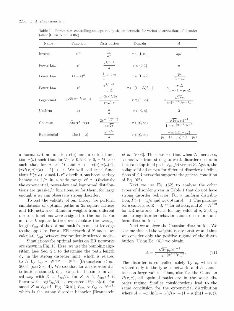
2236 L. A. Braunstein et al.
Table 1. Parameters controlling the optimal paths on networks for various distributions of disorder(after [Chen et al., 2006]).
Name Function Distribution Domain A
Inverse eax 1
aττ ∈ [1, ea] apc
Power Law xa τ1/a−1
aτ ∈ (0, 1] a
Power Law (1 − x)a1
aτ1+1/a τ ∈ [1,∞] a
pc
1 − pc
Power Law xa τ1/a−1
|a|∆ τ ∈ [(1 − ∆)a, 1] apc∆
1 − (1 − pc)∆
Lognormal e√
2a erf−1(2x−1) e−(lnτ)2/2a2
τa√
2πτ ∈ (0,∞) a
√2πpc
e−[erf−1(2pc−1)]2
Uniform ax1
aτ ∈ [0, a] 2
Gaussian√
2a erf−1(x)2e−τ2/(2a2)
a√
2πτ ∈ [0,∞)
√2πpcerf
−1
1 − e−[erf−1(pc)]2
Exponential −a ln(1 − x)e−τ/a
aτ ∈ [0,∞)
−pc ln(1 − pc)
pc + (1 − pc)ln(1 − pc)
a normalization function c(a) and a cutoff func-tion τ(a) such that for ∀ ε > 0,∀E > 0, ∃M > 0such that for a > M and τ ∈ [τ(a), τ(a)E],|τP (τ, a)c(a) − 1| < ε. We will call such func-tions P (τ, a) “quasi-1/τ” distributions because theybehave as 1/τ in a wide range of τ . Obviouslythe exponential, power-law and lognormal distribu-tions are quasi-1/τ functions, so for them, for largeenough a we can observe a strong disorder.
To test the validity of our theory, we performsimulations of optimal paths in 2d square latticesand ER networks. Random weights from differentdisorder functions were assigned to the bonds. Foran L × L square lattice, we calculate the averagelength �opt of the optimal path from one lattice edgeto the opposite. For an ER network of N nodes, wecalculate �opt between two randomly selected nodes.
Simulations for optimal paths on ER networksare shown in Fig. 13. Here, we use the bombing algo-rithm (see Sec. 2.4 to determine the path length�∞ in the strong disorder limit, which is relatedto N by �∞ ∼ Nνopt = N1/3 [Braunstein et al.,2003] (see Sec. 4). We see that for all disorder dis-tributions studied, �opt scales in the same univer-sal way with Z ≡ �∞/A. For Z � 1, �opt/A islinear with log(�∞/A) as expected [Fig. 3(a)]. Forsmall Z = �∞/A [Fig. 13(b)], �opt ∝ �∞ ∼ N1/3,which is the strong disorder behavior [Braunstein
et al., 2003]. Thus, we see that when N increases,a crossover from strong to weak disorder occurs inthe scaled optimal paths �opt/A versus Z. Again, thecollapse of all curves for different disorder distribu-tions of ER networks supports the general conditionof Eq. (62).
Next we use Eq. (62) to analyze the othertypes of disorder given in Table 1 that do not havestrong disorder behavior. For a uniform distribu-tion, P (τ) = 1/a and we obtain A = 1. The parame-ter a cancels, so Z = L1/ν for lattices, and Z = N1/3
for ER networks. Hence for any value of a, Z � 1,and strong disorder behavior cannot occur for a uni-form distribution.
Next we analyze the Gaussian distribution. Weassume that all the weights τj are positive and thuswe consider only the positive regime of the distri-bution. Using Eq. (61) we obtain
A =√
2πpcerf−1
1 − e−[erf−1(pc)]2. (71)
The disorder is controlled solely by pc which isrelated only to the type of network, and A cannottake on large values. Thus, also for the GaussianP (τ, a), all optimal paths are in the weak dis-order regime. Similar considerations lead to thesame conclusion for the exponential distributionwhere A = −pc ln(1 − pc)/(pc + (1 − pc)ln(1 − pc)).
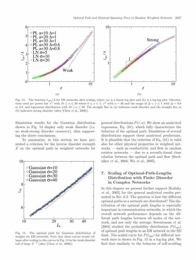
Optimal Path and Minimal Spanning Trees in Random Weighted Networks 2237
1 10Z
0
1
2
3
4
5
6l o
pt /
A
PL a=10 ∆=1PL a=20 ∆=1PL a=30 ∆=1PL a=30 ∆=0.6PL a=30 ∆=0.8LN σ=5LN σ=10LN σ=20
Weak
1 10Z
1
10
l opt
/ A
1
Strong
(a) (b)
Fig. 13. The function �opt/A for ER networks after scaling, where (a) is a linear-log plot and (b) is a log-log plot. Distribu-tions used are power law xa with 10 ≤ a ≤ 30 where 0 ≤ x < 1, xa with a = 30 and the range of ∆ < x ≤ 1 with ∆ = 0.6or 0.8, and lognormal distribution with 10 ≤ a ≤ 30. The straight line in (a) indicates weak disorder and the straight line in(b) indicates strong disorder (after [Chen et al., 2006]).
Simulation results for the Gaussian distributionshown in Fig. 14 display only weak disorder (i.e.no weak-strong disorder crossover), thus support-ing the above conclusions.
To summarize, in this section we have pre-sented a criterion for the inverse disorder strengthZ on the optimal path in weighted networks for
10 20 30 40l 8
6
8
10
l opt
Gaussian σ=10Gaussian σ=20Gaussian σ=30Gaussian σ=40
Fig. 14. The optimal path for Gaussian distribution ofweights for ER networks. Note that these curves would col-lapse after scaling to the curves in Fig. 13 in the weak disordertail of large Z−1 (after [Chen et al., 2006]).
general distributions P (τ, a). We show an analyticalexpression, Eq. (61), which fully characterizes thebehavior of the optimal path. Simulation of severaldistributions support these analytical predictions.It is plausible that the criterion of Eq. (61) is validalso for other physical properties in weighted net-works — such as conductivity and flow in randomresistor networks — due to a recently-found closerelation between the optimal path and flow [Strel-niker et al., 2004; Wu et al., 2005].
7. Scaling of Optimal-Path-LengthsDistribution with Finite Disorderin Complex Networks
In this chapter we present further support [Kaliskyet al., 2005] for the general analytical results pre-sented in Sec. 6.2. The question is how the differentoptimal paths in a network are distributed? The dis-tribution of the optimal path lengths is especiallyimportant in communication networks, in which theoverall network performance depends on the dif-ferent path lengths between all nodes of the net-work, and not only the average. Sreenivasan et al.[2004] studied the probability distribution P (�opt)of optimal path lengths in an ER network in the SDlimit. The scaled curve for P (�opt) for different net-work sizes is shown in Fig. 15 in a log-log plot. Wefind that similarly to the behavior of self-avoiding
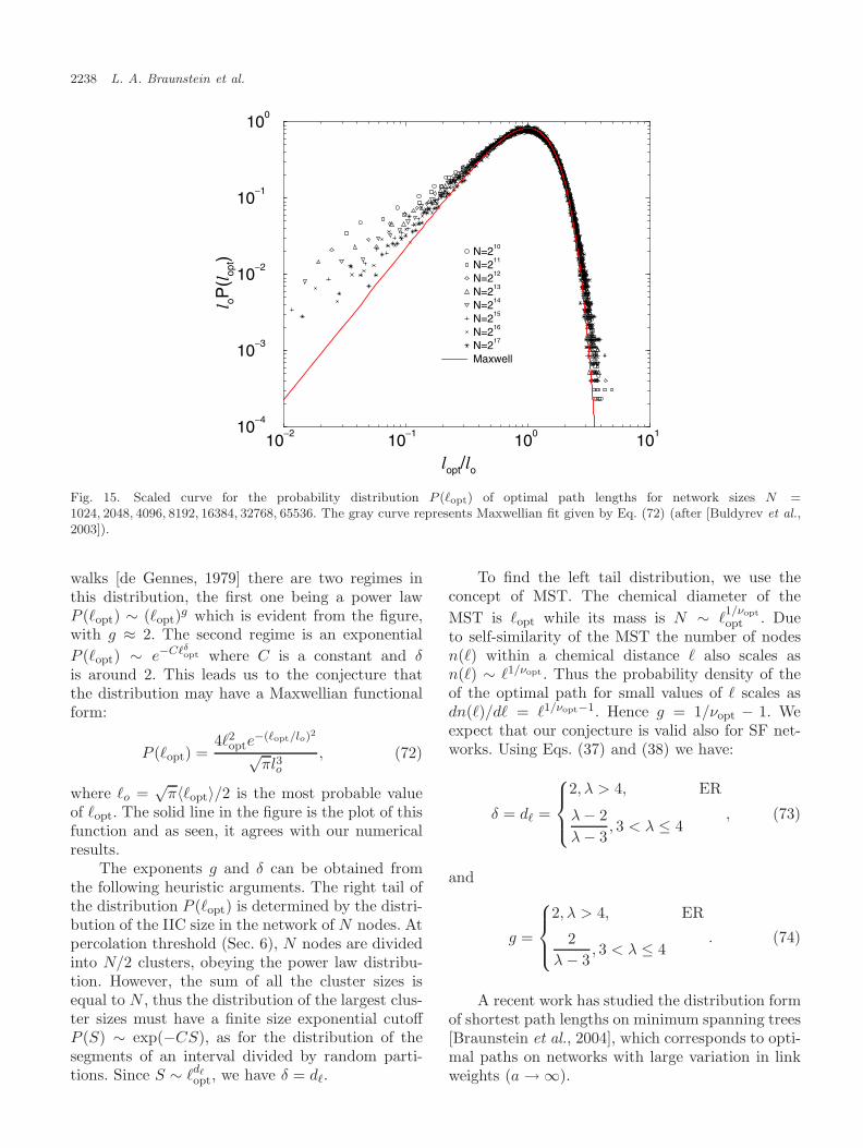
2238 L. A. Braunstein et al.
10−2
10−1
100
101
lopt/lo
10−4
10−3
10−2
10−1
100
l oP(l
opt) N=2
10
N=211
N=212
N=213
N=214
N=215
N=216
N=217
Maxwell
Fig. 15. Scaled curve for the probability distribution P (�opt) of optimal path lengths for network sizes N =1024, 2048, 4096, 8192, 16384, 32768, 65536. The gray curve represents Maxwellian fit given by Eq. (72) (after [Buldyrev et al.,2003]).
walks [de Gennes, 1979] there are two regimes inthis distribution, the first one being a power lawP (�opt) ∼ (�opt)g which is evident from the figure,with g ≈ 2. The second regime is an exponentialP (�opt) ∼ e−C�δ
opt where C is a constant and δis around 2. This leads us to the conjecture thatthe distribution may have a Maxwellian functionalform:
P (�opt) =4�2
opte−(�opt/lo)2
√πl3o
, (72)
where �o =√
π〈�opt〉/2 is the most probable valueof �opt. The solid line in the figure is the plot of thisfunction and as seen, it agrees with our numericalresults.
The exponents g and δ can be obtained fromthe following heuristic arguments. The right tail ofthe distribution P (�opt) is determined by the distri-bution of the IIC size in the network of N nodes. Atpercolation threshold (Sec. 6), N nodes are dividedinto N/2 clusters, obeying the power law distribu-tion. However, the sum of all the cluster sizes isequal to N , thus the distribution of the largest clus-ter sizes must have a finite size exponential cutoffP (S) ∼ exp(−CS), as for the distribution of thesegments of an interval divided by random parti-tions. Since S ∼ �d�
opt, we have δ = d�.
To find the left tail distribution, we use theconcept of MST. The chemical diameter of theMST is �opt while its mass is N ∼ �
1/νopt
opt . Dueto self-similarity of the MST the number of nodesn(�) within a chemical distance � also scales asn(�) ∼ �1/νopt . Thus the probability density of theof the optimal path for small values of � scales asdn(�)/d� = �1/νopt−1. Hence g = 1/νopt − 1. Weexpect that our conjecture is valid also for SF net-works. Using Eqs. (37) and (38) we have:
δ = d� =
2, λ > 4, ER
λ − 2λ − 3
, 3 < λ ≤ 4, (73)
and
g =
2, λ > 4, ER
2λ − 3
, 3 < λ ≤ 4. (74)
A recent work has studied the distribution formof shortest path lengths on minimum spanning trees[Braunstein et al., 2004], which corresponds to opti-mal paths on networks with large variation in linkweights (a → ∞).
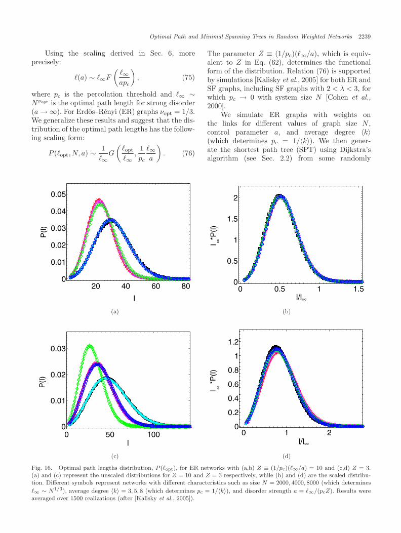
Optimal Path and Minimal Spanning Trees in Random Weighted Networks 2239
Using the scaling derived in Sec. 6, moreprecisely:
�(a) ∼ �∞F
(�∞apc
), (75)
where pc is the percolation threshold and �∞ ∼Nνopt is the optimal path length for strong disorder(a → ∞). For Erdos–Renyi (ER) graphs νopt = 1/3.We generalize these results and suggest that the dis-tribution of the optimal path lengths has the follow-ing scaling form:
P (�opt, N, a) ∼ 1�∞
G
(�opt
�∞,
1pc
�∞a
). (76)
The parameter Z ≡ (1/pc)(�∞/a), which is equiv-alent to Z in Eq. (62), determines the functionalform of the distribution. Relation (76) is supportedby simulations [Kalisky et al., 2005] for both ER andSF graphs, including SF graphs with 2 < λ < 3, forwhich pc → 0 with system size N [Cohen et al.,2000].
We simulate ER graphs with weights onthe links for different values of graph size N ,control parameter a, and average degree 〈k〉(which determines pc = 1/〈k〉). We then gener-ate the shortest path tree (SPT) using Dijkstra’salgorithm (see Sec. 2.2) from some randomly
20 40 60 800
0.01
0.02
0.03
0.04
0.05
l
P(l)
0 0.5 1 1.50
0.5
1
1.5
2
l/l∞
l ∞*P(l)
(a) (b)
0 50 1000
0.01
0.02
0.03
l
P(l)
0 1 20
0.2
0.4
0.6
0.8
1
1.2
l/l∞
l ∞*P
(l)
(c) (d)
Fig. 16. Optimal path lengths distribution, P (�opt), for ER networks with (a,b) Z ≡ (1/pc)(�∞/a) = 10 and (c,d) Z = 3.(a) and (c) represent the unscaled distributions for Z = 10 and Z = 3 respectively, while (b) and (d) are the scaled distribu-tion. Different symbols represent networks with different characteristics such as size N = 2000, 4000, 8000 (which determines
�∞ ∼ N1/3), average degree 〈k〉 = 3, 5, 8 (which determines pc = 1/〈k〉), and disorder strength a = �∞/(pcZ). Results wereaveraged over 1500 realizations (after [Kalisky et al., 2005]).
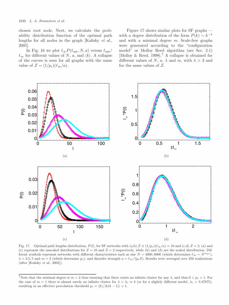
2240 L. A. Braunstein et al.
chosen root node. Next, we calculate the prob-ability distribution function of the optimal pathlengths for all nodes in the graph [Kalisky et al.,2005].
In Fig. 16 we plot �∞P (�opt, N, a) versus �opt/�∞ for different values of N , a, and 〈k〉. A collapseof the curves is seen for all graphs with the samevalue of Z = (1/pc)(�∞/a).
Figure 17 shows similar plots for SF graphs —with a degree distribution of the form P (k) ∼ k−λ
and with a minimal degree m. Scale-free graphswere generated according to the “configurationmodel” or Molloy Reed algorithm (see Sec. 2.1)[Molloy & Reed, 1998].7 A collapse is obtained fordifferent values of N , a, λ and m, with λ > 3 andfor the same values of Z.
0 50 1000
0.01
0.02
0.03
0.04
0.05
0.06
l
P(l)
0 0.5 1 1.50
0.5
1
1.5
l/l∞
l ∞*P
(l)
(a) (b)
0 50 100 1500
0.01
0.02
0.03
l
P(l)
0 1 20
0.2
0.4
0.6
0.8
1
l/l ∞
l ∞*P
(l)
(c) (d)
Fig. 17. Optimal path lengths distribution, P (l), for SF networks with (a,b) Z ≡ (1/pc)(�∞/a) = 10 and (c,d) Z = 2. (a) and(c) represent the unscaled distributions for Z = 10 and Z = 2 respectively, while (b) and (d) are the scaled distribution. Dif-ferent symbols represent networks with different characteristics such as size N = 4000, 8000 (which determines �∞ ∼ Nνopt ),λ = 3.5, 5 and m = 2 (which determine pc), and disorder strength a = �∞/(pcZ). Results were averaged over 250 realizations(after [Kalisky et al., 2005]).
7Note that the minimal degree is m = 2 thus ensuring that there exists an infinite cluster for any λ, and thus 0 < pc < 1. Forthe case of m = 1 there is almost surely no infinite cluster for λ > λc ≈ 4 (or for a slightly different model, λc = 3.47875),resulting in an effective percolation threshold pc = 〈k〉/〈k(k − 1)〉 > 1.
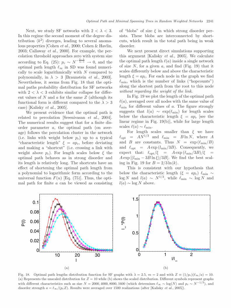
Optimal Path and Minimal Spanning Trees in Random Weighted Networks 2241
Next, we study SF networks with 2 < λ < 3.In this regime the second moment of the degree dis-tribution 〈k2〉 diverges, leading to several anoma-lous properties [Cohen et al., 2000; Cohen & Havlin,2003; Callaway et al., 2000]. For example, the per-colation threshold approaches zero with system sizeaccording to Eq. (25): pc ∼ N− 3−λ
λ−1 → 0, and theoptimal path length �∞ in SD was found numeri-cally to scale logarithmically with N compared topolynomially, in λ > 3 [Braunstein et al., 2003].Nevertheless, it seems from Fig. 18 that the opti-mal paths probability distribution for SF networkswith 2 < λ < 3 exhibits similar collapse for differ-ent values of N and a for the same Z (although itsfunctional form is different compared to the λ > 3case) [Kalisky et al., 2005].
We present evidence that the optimal path isrelated to percolation [Sreenivasan et al., 2004].The numerical results suggest that for a finite dis-order parameter a, the optimal path (on aver-age) follows the percolation cluster in the network(i.e. links with weight below pc) up to a typical“characteristic length” ξ = apc, before deviatingand making a “shortcut” (i.e. crossing a link withweight above pc). For length scales below ξ theoptimal path behaves as in strong disorder andits length is relatively long. The shortcuts have aneffect of shortening the optimal path length froma polynomial to logarithmic form according to theuniversal function F (u) [Eq. (75)]. Thus, the opti-mal path for finite a can be viewed as consisting
of “blobs” of size ξ in which strong disorder per-sists. These blobs are interconnected by short-cuts, which result in the total path being in weakdisorder.
We next present direct simulations supportingthis argument [Kalisky et al., 2005]. We calculatethe optimal path length �(a) inside a single networkof size N , for a given a, and find (Fig. 19) that itscales differently below and above the characteristiclength ξ = apc. For each node in the graph we find�min, which is the number of links (“hopcounts”)along the shortest path from the root to this nodewithout regarding the weight of the link.
In Fig. 19 we plot the length of the optimal path�(a), averaged over all nodes with the same value of�min for different values of a. The figure stronglysuggests that l(a) ∼ exp(�min) for length scalesbelow the characteristic length ξ = apc [see thelinear regime in Fig. 19(b)], while for large lengthscales �(a) ∼ �min.
For length scales smaller than ξ we have�opt = AN1/3 and �min = B ln N , where Aand B are constants. Thus N = exp (�min/B)and �opt = A exp (lmin/3B). Consequently, weexpect that: �opt/ξ = A exp (�min/3B)/ξ =A exp [(lmin − 3B ln ξ)/3B]. We find the best scal-ing in Fig. 19 for B = 2/3 ln〈k〉.
This is consistent with our hypothesis thatbelow the characteristic length (ξ = apc) �min ∼log N and l(a) ∼ N1/3, while �min ∼ log N andl(a) ∼ log N above.
10 20 300
0.02
0.04
0.06
0.08
0.1
l
P(l)
0 1 20
0.5
1
1.5
l/l∞
l ∞*P
(l)
(a) (b)
Fig. 18. Optimal path lengths distribution function for SF graphs with λ = 2.5, m = 2 and with Z ≡ (1/pc)(�∞/a) = 10.(a) Represents the unscaled distribution for Z = 10 while (b) shows the scaled distribution. Different symbols represent graphs
with different characteristics such as size N = 2000, 4000, 8000, 1600 (which determines �∞ ∼ log(N) and pc ∼ N−1/3), anddisorder strength a = �∞/(pcZ). Results were averaged over 1500 realizations (after [Kalisky et al., 2005]).
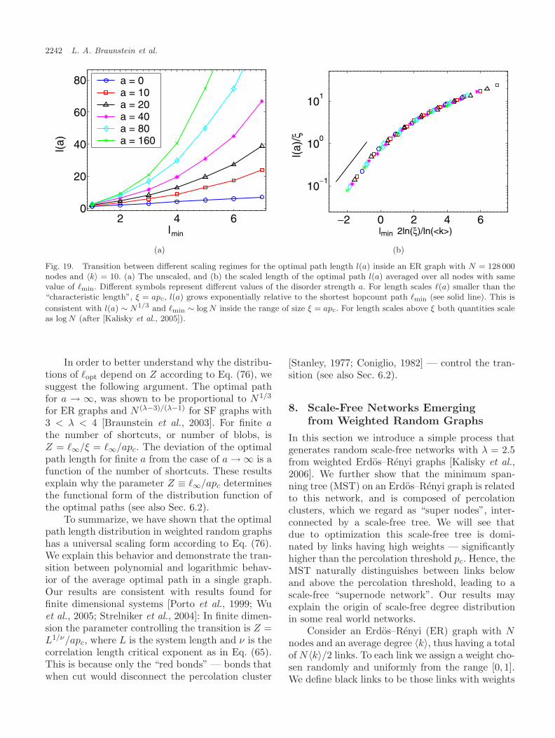
2242 L. A. Braunstein et al.
2 4 60
20
40
60
80
lmin
l(a)
a = 0a = 10a = 20a = 40a = 80a = 160
−2 0 2 4 6
10−1
100
101
lmin 2ln(ξ)/ln(<k>)
l(a)/
ξ
(a) (b)
Fig. 19. Transition between different scaling regimes for the optimal path length l(a) inside an ER graph with N = 128 000nodes and 〈k〉 = 10. (a) The unscaled, and (b) the scaled length of the optimal path l(a) averaged over all nodes with samevalue of �min. Different symbols represent different values of the disorder strength a. For length scales �(a) smaller than the“characteristic length”, ξ = apc, l(a) grows exponentially relative to the shortest hopcount path �min (see solid line). This is
consistent with l(a) ∼ N1/3 and �min ∼ log N inside the range of size ξ = apc. For length scales above ξ both quantities scaleas log N (after [Kalisky et al., 2005]).
In order to better understand why the distribu-tions of �opt depend on Z according to Eq. (76), wesuggest the following argument. The optimal pathfor a → ∞, was shown to be proportional to N1/3
for ER graphs and N (λ−3)/(λ−1) for SF graphs with3 < λ < 4 [Braunstein et al., 2003]. For finite athe number of shortcuts, or number of blobs, isZ = �∞/ξ = �∞/apc. The deviation of the optimalpath length for finite a from the case of a → ∞ is afunction of the number of shortcuts. These resultsexplain why the parameter Z ≡ �∞/apc determinesthe functional form of the distribution function ofthe optimal paths (see also Sec. 6.2).
To summarize, we have shown that the optimalpath length distribution in weighted random graphshas a universal scaling form according to Eq. (76).We explain this behavior and demonstrate the tran-sition between polynomial and logarithmic behav-ior of the average optimal path in a single graph.Our results are consistent with results found forfinite dimensional systems [Porto et al., 1999; Wuet al., 2005; Strelniker et al., 2004]: In finite dimen-sion the parameter controlling the transition is Z =L1/ν/apc, where L is the system length and ν is thecorrelation length critical exponent as in Eq. (65).This is because only the “red bonds” — bonds thatwhen cut would disconnect the percolation cluster
[Stanley, 1977; Coniglio, 1982] — control the tran-sition (see also Sec. 6.2).
8. Scale-Free Networks Emergingfrom Weighted Random Graphs
In this section we introduce a simple process thatgenerates random scale-free networks with λ = 2.5from weighted Erdos–Renyi graphs [Kalisky et al.,2006]. We further show that the minimum span-ning tree (MST) on an Erdos–Renyi graph is relatedto this network, and is composed of percolationclusters, which we regard as “super nodes”, inter-connected by a scale-free tree. We will see thatdue to optimization this scale-free tree is domi-nated by links having high weights — significantlyhigher than the percolation threshold pc. Hence, theMST naturally distinguishes between links belowand above the percolation threshold, leading to ascale-free “supernode network”. Our results mayexplain the origin of scale-free degree distributionin some real world networks.
Consider an Erdos–Renyi (ER) graph with Nnodes and an average degree 〈k〉, thus having a totalof N〈k〉/2 links. To each link we assign a weight cho-sen randomly and uniformly from the range [0, 1].We define black links to be those links with weights
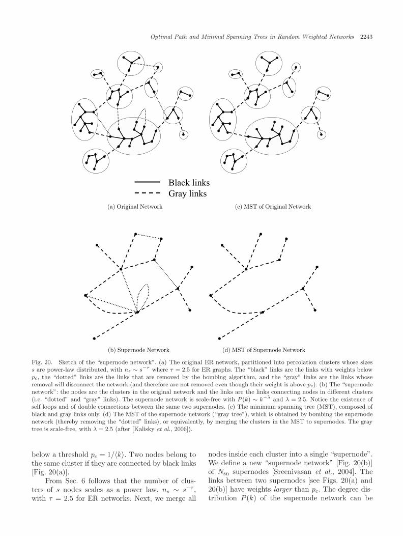
Optimal Path and Minimal Spanning Trees in Random Weighted Networks 2243
Fig. 20. Sketch of the “supernode network”. (a) The original ER network, partitioned into percolation clusters whose sizess are power-law distributed, with ns ∼ s−τ where τ = 2.5 for ER graphs. The “black” links are the links with weights belowpc, the “dotted” links are the links that are removed by the bombing algorithm, and the “gray” links are the links whoseremoval will disconnect the network (and therefore are not removed even though their weight is above pc). (b) The “supernodenetwork”: the nodes are the clusters in the original network and the links are the links connecting nodes in different clusters(i.e. “dotted” and “gray” links). The supernode network is scale-free with P (k) ∼ k−λ and λ = 2.5. Notice the existence ofself loops and of double connections between the same two supernodes. (c) The minimum spanning tree (MST), composed ofblack and gray links only. (d) The MST of the supernode network (“gray tree”), which is obtained by bombing the supernodenetwork (thereby removing the “dotted” links), or equivalently, by merging the clusters in the MST to supernodes. The graytree is scale-free, with λ = 2.5 (after [Kalisky et al., 2006]).
below a threshold pc = 1/〈k〉. Two nodes belong tothe same cluster if they are connected by black links[Fig. 20(a)].
From Sec. 6 follows that the number of clus-ters of s nodes scales as a power law, ns ∼ s−τ ,with τ = 2.5 for ER networks. Next, we merge all
nodes inside each cluster into a single “supernode”.We define a new “supernode network” [Fig. 20(b)]of Nsn supernodes [Sreenivasan et al., 2004]. Thelinks between two supernodes [see Figs. 20(a) and20(b)] have weights larger than pc. The degree dis-tribution P (k) of the supernode network can be
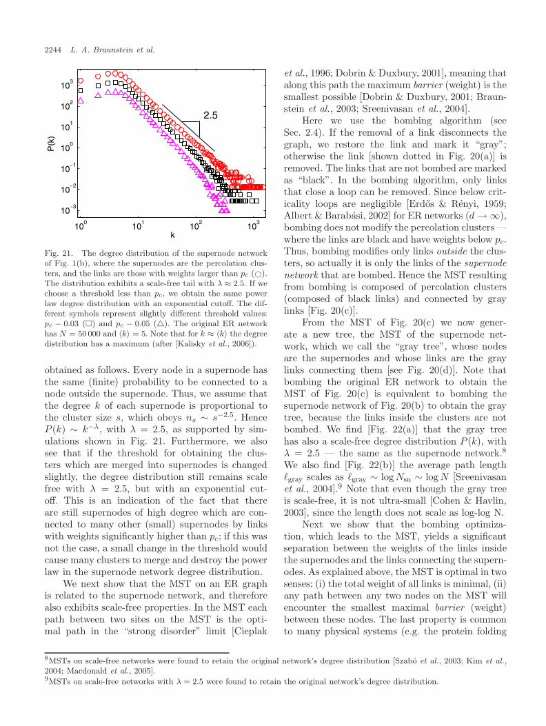
2244 L. A. Braunstein et al.
100
101
102
103
10−3
10−2
10−1
100
101
102
103
k
P(k
)
2.5
Fig. 21. The degree distribution of the supernode networkof Fig. 1(b), where the supernodes are the percolation clus-ters, and the links are those with weights larger than pc (©).The distribution exhibits a scale-free tail with λ ≈ 2.5. If wechoose a threshold less than pc, we obtain the same powerlaw degree distribution with an exponential cutoff. The dif-ferent symbols represent slightly different threshold values:pc − 0.03 (�) and pc − 0.05 (�). The original ER networkhas N = 50 000 and 〈k〉 = 5. Note that for k ≈ 〈k〉 the degreedistribution has a maximum (after [Kalisky et al., 2006]).
obtained as follows. Every node in a supernode hasthe same (finite) probability to be connected to anode outside the supernode. Thus, we assume thatthe degree k of each supernode is proportional tothe cluster size s, which obeys ns ∼ s−2.5. HenceP (k) ∼ k−λ, with λ = 2.5, as supported by sim-ulations shown in Fig. 21. Furthermore, we alsosee that if the threshold for obtaining the clus-ters which are merged into supernodes is changedslightly, the degree distribution still remains scalefree with λ = 2.5, but with an exponential cut-off. This is an indication of the fact that thereare still supernodes of high degree which are con-nected to many other (small) supernodes by linkswith weights significantly higher than pc; if this wasnot the case, a small change in the threshold wouldcause many clusters to merge and destroy the powerlaw in the supernode network degree distribution.
We next show that the MST on an ER graphis related to the supernode network, and thereforealso exhibits scale-free properties. In the MST eachpath between two sites on the MST is the opti-mal path in the “strong disorder” limit [Cieplak
et al., 1996; Dobrin & Duxbury, 2001], meaning thatalong this path the maximum barrier (weight) is thesmallest possible [Dobrin & Duxbury, 2001; Braun-stein et al., 2003; Sreenivasan et al., 2004].
Here we use the bombing algorithm (seeSec. 2.4). If the removal of a link disconnects thegraph, we restore the link and mark it “gray”;otherwise the link [shown dotted in Fig. 20(a)] isremoved. The links that are not bombed are markedas “black”. In the bombing algorithm, only linksthat close a loop can be removed. Since below crit-icality loops are negligible [Erdos & Renyi, 1959;Albert & Barabasi, 2002] for ER networks (d → ∞),bombing does not modify the percolation clusters —where the links are black and have weights below pc.Thus, bombing modifies only links outside the clus-ters, so actually it is only the links of the supernodenetwork that are bombed. Hence the MST resultingfrom bombing is composed of percolation clusters(composed of black links) and connected by graylinks [Fig. 20(c)].
From the MST of Fig. 20(c) we now gener-ate a new tree, the MST of the supernode net-work, which we call the “gray tree”, whose nodesare the supernodes and whose links are the graylinks connecting them [see Fig. 20(d)]. Note thatbombing the original ER network to obtain theMST of Fig. 20(c) is equivalent to bombing thesupernode network of Fig. 20(b) to obtain the graytree, because the links inside the clusters are notbombed. We find [Fig. 22(a)] that the gray treehas also a scale-free degree distribution P (k), withλ = 2.5 — the same as the supernode network.8
We also find [Fig. 22(b)] the average path length�gray scales as �gray ∼ log Nsn ∼ log N [Sreenivasanet al., 2004].9 Note that even though the gray treeis scale-free, it is not ultra-small [Cohen & Havlin,2003], since the length does not scale as log-log N.
Next we show that the bombing optimiza-tion, which leads to the MST, yields a significantseparation between the weights of the links insidethe supernodes and the links connecting the supern-odes. As explained above, the MST is optimal in twosenses: (i) the total weight of all links is minimal, (ii)any path between any two nodes on the MST willencounter the smallest maximal barrier (weight)between these nodes. The last property is commonto many physical systems (e.g. the protein folding
8MSTs on scale-free networks were found to retain the original network’s degree distribution [Szabo et al., 2003; Kim et al.,2004; Macdonald et al., 2005].9MSTs on scale-free networks with λ = 2.5 were found to retain the original network’s degree distribution.
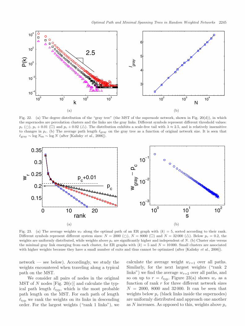
Optimal Path and Minimal Spanning Trees in Random Weighted Networks 2245
100
101
102
103
10−4
10−2
100
102
104
k
P(k
)
2.5
102
103
104
3
4
5
6
N
l gray
(a) (b)
Fig. 22. (a) The degree distribution of the “gray tree” (the MST of the supernode network, shown in Fig. 20(d)), in whichthe supernodes are percolation clusters and the links are the gray links. Different symbols represent different threshold values:pc (©), pc + 0.01 (�) and pc + 0.02 (�). The distribution exhibits a scale-free tail with λ ≈ 2.5, and is relatively insensitiveto changes in pc. (b) The average path length �gray on the gray tree as a function of original network size. It is seen that�gray ∼ log Nsn ∼ log N (after [Kalisky et al., 2006]).
0 10 20
0.15
0.2
0.25
0.3
0.35
rank
wr
pc
pc+0.01
100
101
102
10−3
10−2
10−1
s
wgr
ay−
p c
(a) (b)
Fig. 23. (a) The average weights wr along the optimal path of an ER graph with 〈k〉 = 5, sorted according to their rank.Different symbols represent different system sizes: N = 2000 (©), N = 8000 (�) and N = 32 000 (�). Below pc = 0.2, theweights are uniformly distributed, while weights above pc are significantly higher and independent of N . (b) Cluster size versusthe minimal gray link emerging from each cluster, for ER graphs with 〈k〉 = 5 and N = 10 000. Small clusters are associatedwith higher weights because they have a small number of exits and thus cannot be optimized (after [Kalisky et al., 2006]).
network — see below). Accordingly, we study theweights encountered when traveling along a typicalpath on the MST.
We consider all pairs of nodes in the originalMST of N nodes [Fig. 20(c)] and calculate the typ-ical path length �typ, which is the most probablepath length on the MST. For each path of length�typ we rank the weights on its links in descendingorder. For the largest weights (“rank 1 links”), we
calculate the average weight wr=1 over all paths.Similarly, for the next largest weights (“rank 2links”) we find the average wr=2 over all paths, andso on up to r = �typ. Figure 23(a) shows wr as afunction of rank r for three different network sizesN = 2000, 8000 and 32 000. It can be seen thatweights below pc (black links inside the supernodes)are uniformly distributed and approach one anotheras N increases. As opposed to this, weights above pc
2246 L. A. Braunstein et al.
(“gray links”) are not uniformly distributed, due tothe bombing algorithm, and are independent of N .Actually, weights above pc encountered along theoptimal path (such as the largest weights w1, w2
and w3) are significantly higher than those belowpc. Figure 23(b) shows that the links with the high-est weights on the MST can be associated with graylinks from very small clusters [Figs. 20(a) and 20(c)](similar results have been obtained along the opti-mal path).
As mentioned earlier, this property is presentalso in the original supernode network and hencethe change in the threshold used to obtain thesupernodes does not destroy the power law degreedistribution but only introduces an exponential cut-off. We thereby obtain a scale-free supernode net-work with λ = 2.5, which is not very sensitive tothe precise value of the threshold used for definingthe supernodes. For example, the scale-free degreedistribution shown in Fig. 22(a) for a threshold ofpc + 0.01 corresponds to having only four largestweights on the optimal paths [see Fig. 23(a)]. How-ever, even for pc + 0.02 the degree distribution iswell approximated by a scale-free distribution withλ = 2.5 [see Fig. 22(a)]. This means that mainlyvery small clusters, connected with high-weightlinks to large clusters, dominate the scale-free dis-tribution P (k) of the MST of the supernode net-work (gray tree). Hence, the bombing optimizationprocess on an ER graph causes a significant sepa-ration between links below and above pc to emergespontaneously in the system, and by merging nodesconnected with links of low weights, a scale-free net-work can arise.
The process described above may be related tothe evolution of some real world networks. Considera homogeneous network with many componentswhose average degree 〈k〉 is well defined. Supposethat the links between the components have dif-ferent weights, and that some optimization pro-cess separates the network into nodes which arewell connected (i.e. connected by links with lowweights) and nodes connected by links having muchhigher weights. If the well-connected componentsmerge into a single node, this results in a newheterogeneous supernode network with scale freedegree distribution.
An example of a real world network whose evo-lution may be related to this model is the proteinfolding network, which was found to be scale-free
with λ ≈ 2.3 [Rao, 2004]. The nodes are the pos-sible physical configurations of the system and thelinks between them describe the possible transitionsbetween the different configurations. We assumethat this network is optimal because the systemchooses the path with the smallest energy barrierfrom all possible trajectories in phase space. Itis possible that the scale-free distribution evolvesthrough a similar procedure as described above forrandom graphs: adjacent configurations with closeenergies (nodes in the same cluster) cannot be dis-tinguished and are regarded as a single supernode,while configurations (clusters) with high barriersbetween them belong to different supernodes.
A second example is computer networks.Strongly interacting computers (such as comput-ers belonging to researchers from the same com-pany or research institution) are likely to convergeinto a single domain, and thus domains with varioussizes and connectivities are formed. This networkmight be also optimal, because packets destined toan external domain are presumably routed throughthe router which has the best connection to the tar-get domain.
To summarize, we have seen that any weightedrandom network hides an inherent scale-free“supernode network.”10 We showed that the min-imum spanning tree, generated by the bombingalgorithm, is composed of percolation clusters con-nected by a scale-free tree of “gray” links. Mostof the gray links connect small clusters to largeones, thus having weights well above the percolationthreshold that do not change with the original sizeof the network. Thus the optimization in the processof building the MST distinguishes between linkswith weights below and above the threshold, leadingto a spontaneous emergence of a scale-free “supern-ode network”. We raise the possibility that in somenaturally optimal real-world networks, nodes con-nected well merge into one single node, and thus ascale-free network emerges.
9. Partition of the Minimum SpanningTree into Superhighways and Roads
The centrality, C, quantifies the “importance” ofa node for transport in the network. Moreover,identifying the nodes with high C enables, as shownbelow, to improve their transport capacity and thus
10Similar results can also be obtained for graphs embedded in two or three dimensions, with different power law exponents.
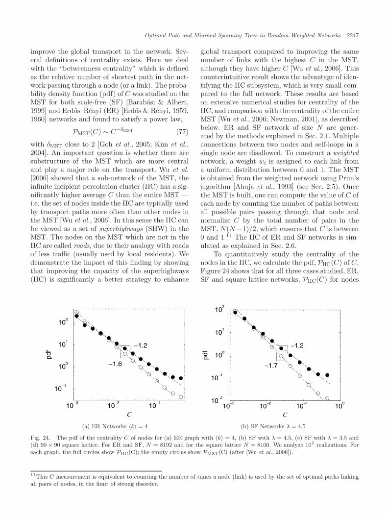
Optimal Path and Minimal Spanning Trees in Random Weighted Networks 2247
improve the global transport in the network. Sev-eral definitions of centrality exists. Here we dealwith the “betweenness centrality” which is definedas the relative number of shortest path in the net-work passing through a node (or a link). The proba-bility density function (pdf) of C was studied on theMST for both scale-free (SF) [Barabasi & Albert,1999] and Erdos–Renyi (ER) [Erdos & Renyi, 1959,1960] networks and found to satisfy a power law,
PMST(C) ∼ C−δMST (77)
with δMST close to 2 [Goh et al., 2005; Kim et al.,2004]. An important question is whether there aresubstructure of the MST which are more centraland play a major role on the transport. Wu et al.[2006] showed that a sub-network of the MST, theinfinite incipient percolation cluster (IIC) has a sig-nificantly higher average C than the entire MST —i.e. the set of nodes inside the IIC are typically usedby transport paths more often than other nodes inthe MST [Wu et al., 2006]. In this sense the IIC canbe viewed as a set of superhighways (SHW) in theMST. The nodes on the MST which are not in theIIC are called roads, due to their analogy with roadsof less traffic (usually used by local residents). Wedemonstrate the impact of this finding by showingthat improving the capacity of the superhighways(IIC) is significantly a better strategy to enhance
global transport compared to improving the samenumber of links with the highest C in the MST,although they have higher C [Wu et al., 2006]. Thiscounterintuitive result shows the advantage of iden-tifying the IIC subsystem, which is very small com-pared to the full network. These results are basedon extensive numerical studies for centrality of theIIC, and comparison with the centrality of the entireMST [Wu et al., 2006; Newman, 2001], as describedbelow. ER and SF network of size N are gener-ated by the methods explained in Sec. 2.1. Multipleconnections between two nodes and self-loops in asingle node are disallowed. To construct a weightednetwork, a weight wi is assigned to each link froma uniform distribution between 0 and 1. The MSTis obtained from the weighted network using Prim’salgorithm [Ahuja et al., 1993] (see Sec. 2.5). Oncethe MST is built, one can compute the value of C ofeach node by counting the number of paths betweenall possible pairs passing through that node andnormalize C by the total number of pairs in theMST, N(N −1)/2, which ensures that C is between0 and 1.11 The IIC of ER and SF networks is sim-ulated as explained in Sec. 2.6.
To quantitatively study the centrality of thenodes in the IIC, we calculate the pdf, PIIC(C) of C.Figure 24 shows that for all three cases studied, ER,SF and square lattice networks, PIIC(C) for nodes
10−3
10−2
10−1
C
10−1
100
101
102
−1.2
−1.6
10−3
10−2
10−1
100
C
10−2
10−1
100
101
102
−1.2
−1.7
(a) ER Networks 〈k〉 = 4 (b) SF Networks λ = 4.5
Fig. 24. The pdf of the centrality C of nodes for (a) ER graph with 〈k〉 = 4, (b) SF with λ = 4.5, (c) SF with λ = 3.5 and(d) 90 × 90 square lattice. For ER and SF, N = 8192 and for the square lattice N = 8100. We analyze 104 realizations. Foreach graph, the full circles show PIIC(C); the empty circles show PMST(C) (after [Wu et al., 2006]).
11This C measurement is equivalent to counting the number of times a node (link) is used by the set of optimal paths linkingall pairs of nodes, in the limit of strong disorder.
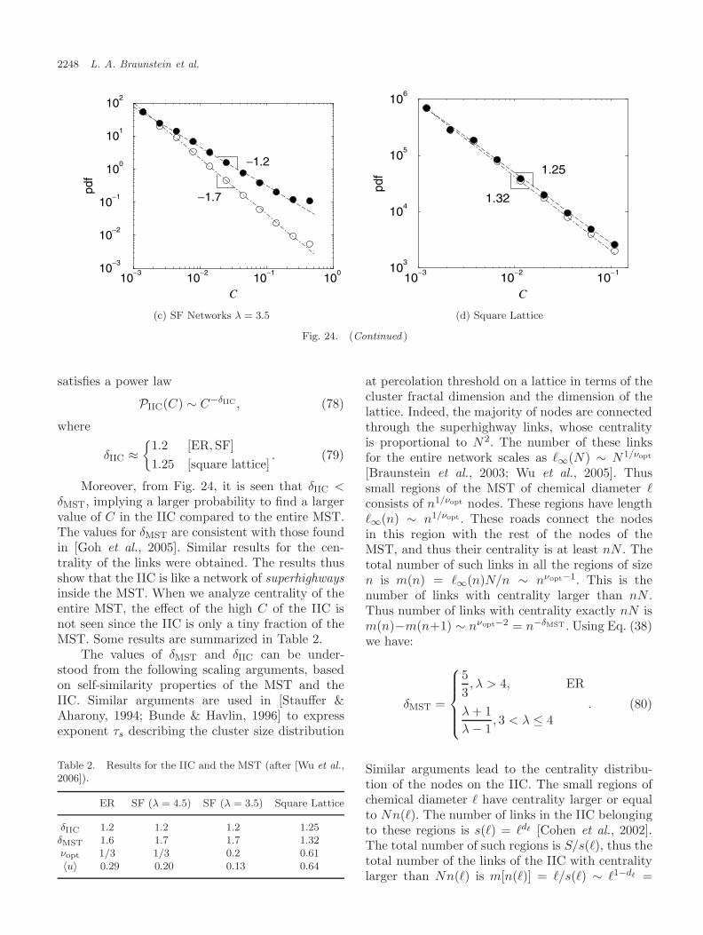
2248 L. A. Braunstein et al.
10−3
10−2
10−1
100
C
10−3
10−2
10−1
100
101
102
−1.2
−1.7
10−3
10−2
10−1
C
103
104
105
106
1.32
1.25
(c) SF Networks λ = 3.5 (d) Square Lattice
Fig. 24. (Continued )
satisfies a power law
PIIC(C) ∼ C−δIIC , (78)
where
δIIC ≈{
1.2 [ER,SF]1.25 [square lattice]
. (79)
Moreover, from Fig. 24, it is seen that δIIC <δMST, implying a larger probability to find a largervalue of C in the IIC compared to the entire MST.The values for δMST are consistent with those foundin [Goh et al., 2005]. Similar results for the cen-trality of the links were obtained. The results thusshow that the IIC is like a network of superhighwaysinside the MST. When we analyze centrality of theentire MST, the effect of the high C of the IIC isnot seen since the IIC is only a tiny fraction of theMST. Some results are summarized in Table 2.
The values of δMST and δIIC can be under-stood from the following scaling arguments, basedon self-similarity properties of the MST and theIIC. Similar arguments are used in [Stauffer &Aharony, 1994; Bunde & Havlin, 1996] to expressexponent τs describing the cluster size distribution
Table 2. Results for the IIC and the MST (after [Wu et al.,2006]).
ER SF (λ = 4.5) SF (λ = 3.5) Square Lattice
δIIC 1.2 1.2 1.2 1.25δMST 1.6 1.7 1.7 1.32νopt 1/3 1/3 0.2 0.61〈u〉 0.29 0.20 0.13 0.64
at percolation threshold on a lattice in terms of thecluster fractal dimension and the dimension of thelattice. Indeed, the majority of nodes are connectedthrough the superhighway links, whose centralityis proportional to N2. The number of these linksfor the entire network scales as �∞(N) ∼ N1/νopt
[Braunstein et al., 2003; Wu et al., 2005]. Thussmall regions of the MST of chemical diameter �consists of n1/νopt nodes. These regions have length�∞(n) ∼ n1/νopt . These roads connect the nodesin this region with the rest of the nodes of theMST, and thus their centrality is at least nN . Thetotal number of such links in all the regions of sizen is m(n) = �∞(n)N/n ∼ nνopt−1. This is thenumber of links with centrality larger than nN .Thus number of links with centrality exactly nN ism(n)−m(n+1) ∼ nνopt−2 = n−δMST . Using Eq. (38)we have:
δMST =
53, λ > 4, ER
λ + 1λ − 1
, 3 < λ ≤ 4. (80)
Similar arguments lead to the centrality distribu-tion of the nodes on the IIC. The small regions ofchemical diameter � have centrality larger or equalto Nn(�). The number of links in the IIC belongingto these regions is s(�) = �d� [Cohen et al., 2002].The total number of such regions is S/s(�), thus thetotal number of the links of the IIC with centralitylarger than Nn(�) is m[n(�)] = �/s(�) ∼ �1−d� =
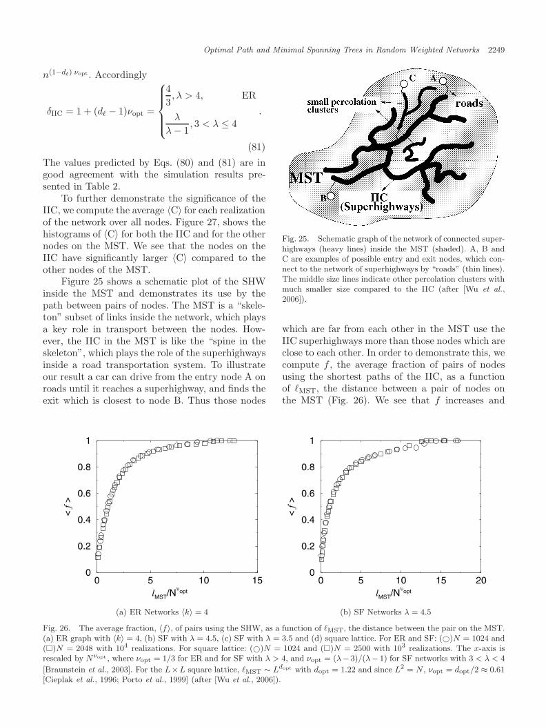
Optimal Path and Minimal Spanning Trees in Random Weighted Networks 2249
n(1−d�) νopt . Accordingly
δIIC = 1 + (d� − 1)νopt =
43, λ > 4, ER
λ
λ − 1, 3 < λ ≤ 4
.
(81)
The values predicted by Eqs. (80) and (81) are ingood agreement with the simulation results pre-sented in Table 2.
To further demonstrate the significance of theIIC, we compute the average 〈C〉 for each realizationof the network over all nodes. Figure 27, shows thehistograms of 〈C〉 for both the IIC and for the othernodes on the MST. We see that the nodes on theIIC have significantly larger 〈C〉 compared to theother nodes of the MST.
Figure 25 shows a schematic plot of the SHWinside the MST and demonstrates its use by thepath between pairs of nodes. The MST is a “skele-ton” subset of links inside the network, which playsa key role in transport between the nodes. How-ever, the IIC in the MST is like the “spine in theskeleton”, which plays the role of the superhighwaysinside a road transportation system. To illustrateour result a car can drive from the entry node A onroads until it reaches a superhighway, and finds theexit which is closest to node B. Thus those nodes
Fig. 25. Schematic graph of the network of connected super-highways (heavy lines) inside the MST (shaded). A, B andC are examples of possible entry and exit nodes, which con-nect to the network of superhighways by “roads” (thin lines).The middle size lines indicate other percolation clusters withmuch smaller size compared to the IIC (after [Wu et al.,2006]).
which are far from each other in the MST use theIIC superhighways more than those nodes which areclose to each other. In order to demonstrate this, wecompute f , the average fraction of pairs of nodesusing the shortest paths of the IIC, as a functionof �MST, the distance between a pair of nodes onthe MST (Fig. 26). We see that f increases and
0 5 10 15lMST/N
υopt
0
0.2
0.4
0.6
0.8
1
< f>
0 5 10 15 20lMST/N
υopt
0
0.2
0.4
0.6
0.8
1
< f>
(a) ER Networks 〈k〉 = 4 (b) SF Networks λ = 4.5
Fig. 26. The average fraction, 〈f〉, of pairs using the SHW, as a function of �MST, the distance between the pair on the MST.(a) ER graph with 〈k〉 = 4, (b) SF with λ = 4.5, (c) SF with λ = 3.5 and (d) square lattice. For ER and SF: (©)N = 1024 and(�)N = 2048 with 104 realizations. For square lattice: (©)N = 1024 and (�)N = 2500 with 103 realizations. The x-axis isrescaled by Nνopt , where νopt = 1/3 for ER and for SF with λ > 4, and νopt = (λ− 3)/(λ− 1) for SF networks with 3 < λ < 4
[Braunstein et al., 2003]. For the L×L square lattice, �MST ∼ Ldopt with dopt = 1.22 and since L2 = N , νopt = dopt/2 ≈ 0.61[Cieplak et al., 1996; Porto et al., 1999] (after [Wu et al., 2006]).
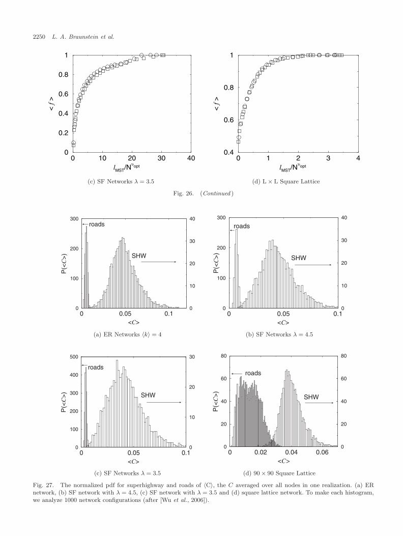
2250 L. A. Braunstein et al.
0 10 20 30 40lMST/N
υopt
0
0.2
0.4
0.6
0.8
1<
f>
0 1 2 3 4lMST/N
υopt
0.4
0.6
0.8
1
< f>
(c) SF Networks λ = 3.5 (d) L × L Square Lattice
Fig. 26. (Continued )
0 0.05 0.1<C>
0
100
200
300
P(<
C>
)
0
10
20
30
40roads
SHW
0 0.05 0.1<C>
0
100
200
300P
(<C
>)
0
10
20
30
40
roads
SHW
(a) ER Networks 〈k〉 = 4 (b) SF Networks λ = 4.5
0 0.05 0.1<C>
0
100
200
300
400
500
P(<
C>
)
0
10
20
30
roads
SHW
0 0.02 0.04 0.06<C>
0
20
40
60
80
P(<
C>
)
0
20
40
60
80
roads
SHW
(c) SF Networks λ = 3.5 (d) 90 × 90 Square Lattice
Fig. 27. The normalized pdf for superhighway and roads of 〈C〉, the C averaged over all nodes in one realization. (a) ERnetwork, (b) SF network with λ = 4.5, (c) SF network with λ = 3.5 and (d) square lattice network. To make each histogram,we analyze 1000 network configurations (after [Wu et al., 2006]).
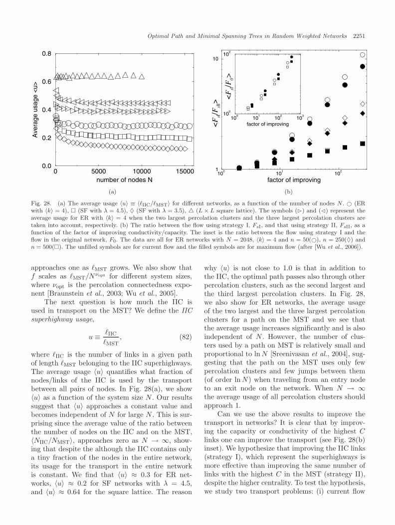
Optimal Path and Minimal Spanning Trees in Random Weighted Networks 2251
0 5000 10000 15000number of nodes N
0.0
0.2
0.4
0.6
0.8
Ave
rage
usa
ge <
u>
100
101
102
factor of improving
1
10
<FsI/F
sII>
100
101
102
103
factor of improving
100
102
<FsI/F
0>
(a) (b)
Fig. 28. (a) The average usage 〈u〉 ≡ 〈�IIC/�MST〉 for different networks, as a function of the number of nodes N . © (ERwith 〈k〉 = 4), � (SF with λ = 4.5), ♦ (SF with λ = 3.5), � (L × L square lattice). The symbols (�) and (�) represent theaverage usage for ER with 〈k〉 = 4 when the two largest percolation clusters and the three largest percolation clusters aretaken into account, respectively. (b) The ratio between the flow using strategy I, FsI, and that using strategy II, FsII, as afunction of the factor of improving conductivity/capacity. The inset is the ratio between the flow using strategy I and theflow in the original network, F0. The data are all for ER networks with N = 2048, 〈k〉 = 4 and n = 50(©), n = 250(♦) andn = 500(�). The unfilled symbols are for current flow and the filled symbols are for maximum flow (after [Wu et al., 2006]).
approaches one as �MST grows. We also show thatf scales as �MST/Nνopt for different system sizes,where νopt is the percolation connectedness expo-nent [Braunstein et al., 2003; Wu et al., 2005].
The next question is how much the IIC isused in transport on the MST? We define the IICsuperhighway usage,
u ≡ �IIC
�MST, (82)
where �IIC is the number of links in a given pathof length �MST belonging to the IIC superhighways.The average usage 〈u〉 quantifies what fraction ofnodes/links of the IIC is used by the transportbetween all pairs of nodes. In Fig. 28(a), we show〈u〉 as a function of the system size N . Our resultssuggest that 〈u〉 approaches a constant value andbecomes independent of N for large N . This is sur-prising since the average value of the ratio betweenthe number of nodes on the IIC and on the MST,〈NIIC/NMST〉, approaches zero as N → ∞, show-ing that despite the although the IIC contains onlya tiny fraction of the nodes in the entire network,its usage for the transport in the entire networkis constant. We find that 〈u〉 ≈ 0.3 for ER net-works, 〈u〉 ≈ 0.2 for SF networks with λ = 4.5,and 〈u〉 ≈ 0.64 for the square lattice. The reason
why 〈u〉 is not close to 1.0 is that in addition tothe IIC, the optimal path passes also through otherpercolation clusters, such as the second largest andthe third largest percolation clusters. In Fig. 28,we also show for ER networks, the average usageof the two largest and the three largest percolationclusters for a path on the MST and we see thatthe average usage increases significantly and is alsoindependent of N . However, the number of clus-ters used by a path on MST is relatively small andproportional to ln N [Sreenivasan et al., 2004], sug-gesting that the path on the MST uses only fewpercolation clusters and few jumps between them(of order ln N) when traveling from an entry nodeto an exit node on the network. When N → ∞the average usage of all percolation clusters shouldapproach 1.
Can we use the above results to improve thetransport in networks? It is clear that by improv-ing the capacity or conductivity of the highest Clinks one can improve the transport (see Fig. 28(b)inset). We hypothesize that improving the IIC links(strategy I), which represent the superhighways ismore effective than improving the same number oflinks with the highest C in the MST (strategy II),despite the higher centrality. To test the hypothesis,we study two transport problems: (i) current flow
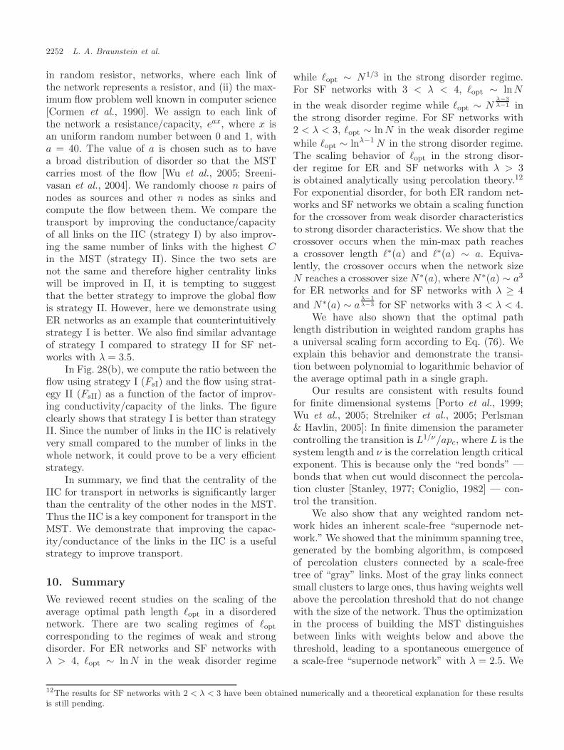
2252 L. A. Braunstein et al.
in random resistor, networks, where each link ofthe network represents a resistor, and (ii) the max-imum flow problem well known in computer science[Cormen et al., 1990]. We assign to each link ofthe network a resistance/capacity, eax, where x isan uniform random number between 0 and 1, witha = 40. The value of a is chosen such as to havea broad distribution of disorder so that the MSTcarries most of the flow [Wu et al., 2005; Sreeni-vasan et al., 2004]. We randomly choose n pairs ofnodes as sources and other n nodes as sinks andcompute the flow between them. We compare thetransport by improving the conductance/capacityof all links on the IIC (strategy I) by also improv-ing the same number of links with the highest Cin the MST (strategy II). Since the two sets arenot the same and therefore higher centrality linkswill be improved in II, it is tempting to suggestthat the better strategy to improve the global flowis strategy II. However, here we demonstrate usingER networks as an example that counterintuitivelystrategy I is better. We also find similar advantageof strategy I compared to strategy II for SF net-works with λ = 3.5.
In Fig. 28(b), we compute the ratio between theflow using strategy I (FsI) and the flow using strat-egy II (FsII) as a function of the factor of improv-ing conductivity/capacity of the links. The figureclearly shows that strategy I is better than strategyII. Since the number of links in the IIC is relativelyvery small compared to the number of links in thewhole network, it could prove to be a very efficientstrategy.
In summary, we find that the centrality of theIIC for transport in networks is significantly largerthan the centrality of the other nodes in the MST.Thus the IIC is a key component for transport in theMST. We demonstrate that improving the capac-ity/conductance of the links in the IIC is a usefulstrategy to improve transport.
10. Summary
We reviewed recent studies on the scaling of theaverage optimal path length �opt in a disorderednetwork. There are two scaling regimes of �opt
corresponding to the regimes of weak and strongdisorder. For ER networks and SF networks withλ > 4, �opt ∼ ln N in the weak disorder regime
while �opt ∼ N1/3 in the strong disorder regime.For SF networks with 3 < λ < 4, �opt ∼ lnN
in the weak disorder regime while �opt ∼ Nλ−3λ−1 in
the strong disorder regime. For SF networks with2 < λ < 3, �opt ∼ ln N in the weak disorder regimewhile �opt ∼ lnλ−1 N in the strong disorder regime.The scaling behavior of �opt in the strong disor-der regime for ER and SF networks with λ > 3is obtained analytically using percolation theory.12
For exponential disorder, for both ER random net-works and SF networks we obtain a scaling functionfor the crossover from weak disorder characteristicsto strong disorder characteristics. We show that thecrossover occurs when the min-max path reachesa crossover length �∗(a) and �∗(a) ∼ a. Equiva-lently, the crossover occurs when the network sizeN reaches a crossover size N∗(a), where N∗(a) ∼ a3
for ER networks and for SF networks with λ ≥ 4and N∗(a) ∼ a
λ−1λ−3 for SF networks with 3 < λ < 4.
We have also shown that the optimal pathlength distribution in weighted random graphs hasa universal scaling form according to Eq. (76). Weexplain this behavior and demonstrate the transi-tion between polynomial to logarithmic behavior ofthe average optimal path in a single graph.
Our results are consistent with results foundfor finite dimensional systems [Porto et al., 1999;Wu et al., 2005; Strelniker et al., 2005; Perlsman& Havlin, 2005]: In finite dimension the parametercontrolling the transition is L1/ν/apc, where L is thesystem length and ν is the correlation length criticalexponent. This is because only the “red bonds” —bonds that when cut would disconnect the percola-tion cluster [Stanley, 1977; Coniglio, 1982] — con-trol the transition.
We also show that any weighted random net-work hides an inherent scale-free “supernode net-work.” We showed that the minimum spanning tree,generated by the bombing algorithm, is composedof percolation clusters connected by a scale-freetree of “gray” links. Most of the gray links connectsmall clusters to large ones, thus having weights wellabove the percolation threshold that do not changewith the size of the network. Thus the optimizationin the process of building the MST distinguishesbetween links with weights below and above thethreshold, leading to a spontaneous emergence ofa scale-free “supernode network” with λ = 2.5. We
12The results for SF networks with 2 < λ < 3 have been obtained numerically and a theoretical explanation for these resultsis still pending.
Optimal Path and Minimal Spanning Trees in Random Weighted Networks 2253
raise the possibility that in some naturally optimalreal-world networks, nodes connected well mergeinto one single node, and thus a scale-free networkemerges.
The centrality in networks for transport on theMST is studied. We found that the centrality ofthe nodes in the IIC is significantly larger thanthe centrality of the other nodes in the MST. Theanalytical estimation for the exponents of the cen-trality distribution for both the MST and the IICare provided. Thus the IIC is a key componentfor transport in the MST. As a result of this find-ing, we demonstrated that improving the capacity/conductance of the links in the IIC is a useful strat-egy to improve transport which is a better strategycompared to improving the same number of linkswith the highest centrality in the MST. This is prob-ably due to the global nature of transport which pre-fer global improvement of the superhighways ratherthan local improvement of high centrality links.
Acknowledgments
We thank ONR, Israel Science Foundation, Euro-pean NEST project DYSONET, FONCyt (PICT-O 2004/370) and Israeli Center for ComplexityScience for financial support.
References
Albert, R. & Barabasi, A.-L. [2002] “Statistical mechan-ics of complex networks,” Rev. Mod. Phys. 74, 47–97.
Ahuja, R. K., Magnanti, T. L. & Orlin, J. B. [1993]Network Flows: Theory, Algorithms and Applications(Prentice-Hall, Englewood Cliffs).
Barabasi, A.-L. [1996] “Invasion percolation and globaloptimization,” Phys. Rev. Lett. 76, 3750–3753.
Barabasi, A.-L. & Albert, R. [1999] “Emergence of scal-ing in random networks,” Science 286, 509–512.
Barabasi, A.-L. [2002] Linked: The New Science of Net-works (Perseus Publishing, Cambridge, MA).
Barrat, A. et al. [2004] “The architecture of complexweighted networks,” PNAS 101, 3747–3752.
Barthelemy, M. & Amaral, L. A. N. [1999] “Small-worldnetworks: Evidence for a crossover picture,” Phys.Rev. Lett. 82, 3180–3183.
Boccaletti, S., Latora, V., Moreno, Y., Chavez, M. &Hwang, D.-U. [2006] “Complex networks: Structureand dynamics,” Phys. Rep. 424, 175–308.
Bollobas, B. [1985] Random Graphs (Academic,London).
Bonanno, G., Caldarelli, G., Lillo, F. & Mantegna, R. N.[2003] “Topology of correlation-based minimal span-ning trees in real and model markets,” Phys. Rev. E68, 046130-1–4.
Braunstein, L. A., Buldyrev, S. V., Havlin, S. & Stan-ley, H. E. [2001] “Universality classes for self-avoidingwalks in a strongly disordered system,” Phys. Rev. E65, 056128-1–6.
Braunstein, L. A., Buldyrev, S. V., Cohen, R., Havlin, S.& Stanley, H. E. [2003] “Optimal paths in disorderedcomplex networks,” Phys. Rev. Lett. 91, 168701-1–4.
Braunstein, L. A., Buldyrev, S. V., Sreenivasan, S.,Cohen, R., Havlin, S. & Stanley, H. E. [2004]“The optimal path in a random network,” Lec-ture Notes in Physics: Proc. 23rd CNLS Conf.,“Complex Networks,” Santa Fe 2003, eds. Ben-Naim, E., Frauenfelder, H. & Toroczkai, Z. (Springer,Berlin).
Buchanan, M. [2002] Nexus: Small Worlds and theGroundbreaking Theory of Networks (W. W. Norton,NY).
Buldyrev, S. V., Braunstein, L. A., Cohen, R., Havlin,S. & Stanley, H. E. [2003] “Length of optimal pathin random networks with strong disorder,” Physica A330, 246–252.
Buldyrev, S. V., Havlin, S. & Stanley, H. E. [2006] “Opti-mal paths in strong and weak disorder: A unifiedapproach,” Phys. Rev. E 73, 036128-1–6.
Bunde, A. & Havlin, S. (eds.) [1996] Fractals and Disor-dered Systems (Springer, NY).
Callaway, D. S., Newman, M. E. J., Strogatz, S. H. &Watts, D. J. [2000] “Network robustness and fragility:Percolation on random graphs,” Phys. Rev. Lett. 85,5468–5471.
Chen, Y. et al. [2006] “Universal behavior of optimalpaths in weighted networks with general disorder,”Phys. Rev. Lett. 96, 068702-1–4.
Cieplak, M., Maritan, A. & Banavar, J. R. [1994] “Opti-mal paths and domain walls in the strong disorderlimit,” Phys. Rev. Lett. 72, 2320–2323.
Cieplak, M., Maritan, A. & Banavar, J. R. [1996] “Inva-sion percolation and eden growth: Geometry and uni-versality,” Phys. Rev. Lett. 76, 3754–3757.
Cohen, R., Erez, K., ben-Avraham, D. & Havlin, S.[2000] “Resilience of the Internet to random break-downs,” Phys. Rev. Lett. 85, 4626–4628.
Cohen, R., ben-Avraham, D. & Havlin, S. [2002] “Perco-lation critical exponents in scale-free networks,” Phys.Rev. E 66, 036113-1–4.
Cohen, R., Havlin, S. & ben-Avraham, D. [2002] “Struc-tural properties of scale free networks,” in Handbookof Graphs and Networks, eds. Bornholdt, S. & Shus-ter, H. G. (Willey-VCH, NY), Chap. 4.
Cohen, R. & Havlin, S. [2003] “Scale free networks areultrasmall,” Phys. Rev. Lett. 90, 058701-1–4.
Coniglio, A. [1982] “Cluster structure near the percola-tion threshold,” J. Phys. A 15, 3829–3844.
Cormen, T. H., Leiserson, C. E. & Rivest, R. L. [1990]Introduction to Algorithms (MIT Press, Cambridge,MA).
2254 L. A. Braunstein et al.
de Gennes, P.-G. [1979] Scaling Concepts in PolymerPhysics (Cornell University Press, Ithaca).
Dobrin, R. & Duxbury, P. M. [2001] “Minimum span-ning trees on random networks,” Phys. Rev. Lett. 86,5076–5079.
Dorogovtsev, S. N. & Mendes, J. F. F. [2003] Evolutionof Networks: From Biological Nets to the Internet andWWW (Oxford University Press, Oxford).
Erdos, P. & Renyi, A. [1959] “On random graphs,” Publ.Math. 6, 290–297.
Erdos, P. & Renyi, A. [1960] “On the evolution of ran-dom graphs,” Publ. Math. Inst. Hungarian Acad. Sci.5, 17–61.
Fredman, M. L. & Tarjan, R. E. [1987] “Fibonacci heapsand their uses in improved network optimization algo-rithms,” J. ACM 34, 596–615.
Grassberger, P. & Zhang, Y. C. [1996] “Self-organizedformulation of standard percolation phenomena,”Physica A 224, 169–179.
Goh, K.-I., Kahng, B. & Kim, D. [2001] “Universalbehavior of load distribution in scale-free networks,”Phys. Rev. Lett. 87, 278701-1–4.
Goh, K.-I., Noh, J. D. Kahng, B. & Kim, D. [2005]“Load distribution in weighted complex networks,”Phys. Rev. E 72, 017102-1–4.
Hansen, A. & Kertesz, J. [2004] “Phase diagram of opti-mal paths,” Phys. Rev. Lett. 93, 040601-1–4.
Harris, T. E. [1989] The Theory of Branching Processes(Dover Publication Inc., NY).
Havlin, S., Braunstein, L. A., Buldyrev, S. V., Cohen,R., Kalisky, T., Sreenivasan, S. & Stanley, H. E. [2005]“Optimal paths in random networks with disorder: Amini review,” Physica A 346, 82–92.
Ioselevich, A. S. & Lyubshin, D. S. [2004] “Phase transi-tion in a self-repairing random network,” JETP Lett.79, 231–235.
Kalisky, T., Braunstein, L. A., Buldyrev, S. V., Havlin,S. & Stanley, H. E. [2005] “Scaling of optimal-path-lengths distribution in complex networks,” Phys. Rev.E 72, 025102-1–4(R).
Kalisky, T. & Cohen, R. [2006] “Width of percolationtransition in complex networks,” Phys. Rev. E 73,035101-1–4(R).
Kalisky, T., Sreenivasan, S., Braunstein, L. A., Havlin,S. & Stanley, H. E. [2006] “Scale-free networks emerg-ing from weighted random graphs,” Phys. Rev. E 73,025103-1–4(R).
Khan, M., Pandurangan, G. & Bhargava, B. [2003]“Energy-efficient routing schemes for sensor net-works,” Tech. Rep. CSD TR 03-013, Dept. of Com-puter Science, Purdue University.
Kim, D.-H., Noh, J. D. & Jeong, H. [2004] “Scale-freetrees: The skeletons of complex networks,” Phys. Rev.E 70, 046126-1–5.
Kruskal, J. B. [1956] “On the shortest spanning subtreeand the traveling salesman problem,” Proc. Amer.Math. Soc. 7, 48–50.
Macdonald, P. J., Almaas, E. & Barabasi, A.-L. [2005]“Minimum spanning trees of weighted scale-free net-works,” Europhys. Lett. 72, 308–314.
Mendes, J. F. F., Dorogovtsev, S. N. & Ioffe, A. F.[2003] Evolution of Networks: From Biological Nets tothe Internet and the WWW (Oxford University Press,Oxford).
Molloy, M. & Reed, B. [1995] “A critical-point for ran-dom graphs with a given degree sequence,” Rand.Struct. Algorith. 6, 161–179.
Molloy, M. & Reed, B. [1998] “The size of the giantcomponent of a random graph with a given degreesequence ,” Combin. Probab. Comput. 7, 295–305.
Newman, M. E. J. [2001a] “Scientific collaborationnetworks. I. Network construction and fundamentalresults,” Phys. Rev. E 64, 016131-1–8.
Newman, M. E. J. [2001b] “Scientific collaboration net-works. II. Shortest paths, weighted networks, and cen-trality,” Phys. Rev. E 64, 016132-1–7.
Onnela, J.-P. et al. [2003] “Dynamics of market correla-tions: Taxonomy and portfolio analysis,” Phys. Rev.E 68, 056110-1–12.
Pastor-Satorras, R. & Vespignani, A. [2004] Structureand Evolution of the Internet: A Statistical PhysicsApproach (Cambridge University Press, Cambridge).
Perlsman, E. & Havlin, S. [2005] “Directed polymer —directed percolation transition: The strong disordercase,” Eur. Phys. J. B 43, 517–520.
Perlsman, E. & Havlin, S. [2006] “Optimal paths as cor-related random walks,” Europhys. Lett. 73, 178–182.
Porto, M., Havlin, S., Schwarzer, S. & Bunde, A. [1997]“Optimal path in strong disorder and shortest path ininvasion percolation with trapping,” Phys. Rev. Lett.79, 4060–4062.
Porto, M., Schwartz, N., Havlin, S. & Bunde, A. [1999]“Optimal paths in disordered media: Scaling of thecrossover from self-similar to self-affine behavior,”Phys. Rev. E 60, R2448–R2451.
Rao, A. & Caflisch, F. [2004] “The protein folding net-work,” J. Mol. Biol. 342, 299–306.
Skiena, S. [1990] Implementing Discrete Mathematics:Combinatorics and Graph Theory With Mathematica(Addison-Wesley, NY).
Smailer, I., Machta, J. & Redner, S. [1993] “Exact enu-meration of self-avoiding walks on lattices with ran-dom site energies,” Phys. Rev. E 47, 262–266.
Sreenivasan, S., Kalisky, T., Braunstein, L. A., Buldyrev,S. V., Havlin, S. & Stanley, H. E. [2004] “Effect ofdisorder strength on optimal paths in complex net-works,” Phys. Rev. E 70, 046133-1–6.
Sreenivasan, S., Kalisky, T., Braunstein, L. A.,Buldyrev, S. V., Havlin, S. & Stanley, H. E.[2005] “Transition between strong and weak disor-der regimes on the optimal path,” Physica A 346,174–182.
Stanley, H. E. [1977] “Cluster shapes at the percolationthreshold: An effective cluster dimensionality and its
Optimal Path and Minimal Spanning Trees in Random Weighted Networks 2255
connection with critical-point exponents,” J. Phys. A10, L211–L220.
Stauffer, D. & Aharony, A. [1994] Introduction to Perco-lation Theory (Taylor & Francis, London).
Strelniker, Y. M. et al. [2004] “Percolation transition in atwo-dimensional system of Ni granular ferromagnets,”Phys. Rev. E 69, 065105-1–4(R).
Strelniker, Y. M., Havlin, S., Berkovits, R. & Frydman,A. [2005] “Resistance distribution in the hopping per-colation model,” Phys. Rev. E 72, 016121-1–5.
Szabo, G. J., Alava, M. & Kertesz, J. [2003] “Geometryof minimum spanning trees on scale-free networks,”Physica A 330, 31–36.
van der Hofstad, R., Hooghienstra, G. & van Mieghem,P. [2001] “First passage percolation on the randomgraph,” Prob. Eng. Inf. Sci. 15, 225–237.
Watts, D. J. [2003] Six Degrees: The Science of a Con-nected Age (W. W. Norton, NY).
Wu, Z. et al. [2005] “Current flow in random resistornetworks: The role of percolation in weak and strongdisorder,” Phys. Rev. E 71, 045101-1–4(R).
Wu, Z., Braunstein, L. A., Havlin, S. & Stanley, H.E. [2006] “Transport in weighted networks: Partitioninto superhighways and roads,” Phys. Rev. Lett. 96,148702-1–4.
Related Documents

![[ACM-ICPC] Minimal Spanning Tree](https://static.cupdf.com/doc/110x72/55513e4bb4c905bd1c8b49a8/acm-icpc-minimal-spanning-tree.jpg)