Optimal Partitioning and Coordination Decisions in Decomposition-based Design Optimization by James T. Allison A dissertation submitted in partial fulfillment of the requirements for the degree of Doctor of Philosophy (Mechanical Engineering) in The University of Michigan 2008 Doctoral Committee: Professor Panos Y. Papalambros, Chair Professor Noboru Kikuchi Professor Romesh Saigal Associate Research Scientist Michael Kokkolaras Terrance Wagner, Ford Motor Company

Welcome message from author
This document is posted to help you gain knowledge. Please leave a comment to let me know what you think about it! Share it to your friends and learn new things together.
Transcript

Optimal Partitioning and Coordination Decisions inDecomposition-based Design Optimization
by
James T. Allison
A dissertation submitted in partial fulfillmentof the requirements for the degree of
Doctor of Philosophy(Mechanical Engineering)
in The University of Michigan2008
Doctoral Committee:
Professor Panos Y. Papalambros, ChairProfessor Noboru KikuchiProfessor Romesh SaigalAssociate Research Scientist Michael KokkolarasTerrance Wagner, Ford Motor Company

c© James T. Allison
All Rights Reserved2008

to Ellie, Jonathan, Brian, and Michael
ii

Acknowledgments
I have been very fortunate to study under the masterful guidance of my advisor, PanosPapalambros. I am grateful for his remarkable support throughout my challenges andadventures at the University of Michigan; I have been inspired by his example. It wasbecause of the opportunity to work with him that I chose to come to Michigan, and Iundoubtedly made the right choice. I want to thank my dissertation committee for the timeand effort they volunteered to guide my dissertation work. I want also to recognize my wife,Natalie, who has labored just as ardently as I toward my graduation, and my extended familyand friends, who gave of themselves so that I could realize my ambitions.
Much of my work has been collaborative. Michael Kokkolaras has been a valuable men-tor and research collaborator throughout my graduate studies. Thanks to my affiliation withthe Optimal Design Laboratory at the University of Michigan, I’ve had fantastic opportuni-ties to work with people from around the world, including Brian Roth, Emanuele Colomba,Guido Karsemakers, Simon Tosserams, David Walsh, and others. I want to thank all ofmy ODE friends for enriching my experiences, including Ryan Fellini, Erin MacDonald,Jeongwoo Han, Jarod Kelly, Kwang Jae Lee, Kuei-Yuan Chan, Jeremy Michalek, SubrotoGunawan, Marc Zawislak, Eric Rask, Mike Sasena, Bart Frischknecht, and many others. Iam grateful to my other friends at the U of M, including Mike Cherry, April Bryan, NatashaChang, Eduardo Izquierdo, Brian Trease, Ken Pollary, and others.
Many individuals contributed to the electric vehicle design case study. Kwang Jae Leeplayed an important role in system integration, optimization, and programming. JeongwooHan provided the Li-ion battery model, and Jarod Kelley developed the frame design andstructural model. Emanuele Colomba helped define chassis design and overall vehiclegeometry. Michael Alexander assisted with structural model development. DushyantWadivkar, Burit Kitterungsi, and Mikael Nybacka all provided support for the vehicledynamics model, and Hisashi Heguri generously furnished tire model data.
Many experiences helped prepare me for graduate school. My involvement with the solarcar team at the University of Utah not only helped me discover my research interests, butgave me glimpses of the possible. My fellow solar car teammates, including Andy Rahden,Jayme Allred, Tadd Truscott, and Brad Hansen, played a vital role. Eberhard Bamberg,also of the University of Utah, was an important mentor who offered timely direction and
iii

encouraged me to seek the best possible graduate school experience. Dennis Rosier, my highschool auto shop teacher, helped ignite my passion for learning, and Corinne Barney, myhigh school math teacher, inspired me to expand my horizons. My parents offered regularencouragement to live to my potential, and my father provided long hours of math tutoringthrough my early college years that were key to my academic success.
Finally, I would like to recognize support from the U.S. National Science Foundation, theAutomotive Research Center at the University of Michigan, the Rackham Graduate School,and the University of Michigan College of Engineering and Department of MechanicalEngineering.
iv

Table of Contents
Dedication . . . . . . . . . . . . . . . . . . . . . . . . . . . . . . . . . . . . . . . ii
Acknowledgments . . . . . . . . . . . . . . . . . . . . . . . . . . . . . . . . . . . iii
List of Tables . . . . . . . . . . . . . . . . . . . . . . . . . . . . . . . . . . . . . . viii
List of Figures . . . . . . . . . . . . . . . . . . . . . . . . . . . . . . . . . . . . . ix
List of Symbols . . . . . . . . . . . . . . . . . . . . . . . . . . . . . . . . . . . . . xii
Abstract . . . . . . . . . . . . . . . . . . . . . . . . . . . . . . . . . . . . . . . . . xv
Chapter 1 Decomposition-based Design Optimization . . . . . . . . . . . . . . 11.1 Engineering System Design . . . . . . . . . . . . . . . . . . . . . . . . . . 21.2 Design Optimization . . . . . . . . . . . . . . . . . . . . . . . . . . . . . 41.3 Decomposition-based Design Optimization . . . . . . . . . . . . . . . . . 81.4 Introductory Example . . . . . . . . . . . . . . . . . . . . . . . . . . . . . 11
1.4.1 Coordination Decisions . . . . . . . . . . . . . . . . . . . . . . . . 131.4.2 Partitioning Decisions . . . . . . . . . . . . . . . . . . . . . . . . 15
1.5 Dissertation Overview . . . . . . . . . . . . . . . . . . . . . . . . . . . . 16
Chapter 2 Partitioning and Coordination Decisions . . . . . . . . . . . . . . . 182.1 Decomposition-based System Design . . . . . . . . . . . . . . . . . . . . 18
2.1.1 System Consistency . . . . . . . . . . . . . . . . . . . . . . . . . 202.1.2 System Optimality . . . . . . . . . . . . . . . . . . . . . . . . . . 202.1.3 Distributed Optimization . . . . . . . . . . . . . . . . . . . . . . . 21
2.2 Decision Framework . . . . . . . . . . . . . . . . . . . . . . . . . . . . . 222.3 System Representation . . . . . . . . . . . . . . . . . . . . . . . . . . . . 24
2.3.1 Structural Matrix . . . . . . . . . . . . . . . . . . . . . . . . . . . 242.3.2 Design Structure Matrix . . . . . . . . . . . . . . . . . . . . . . . 252.3.3 Other Design Matrices . . . . . . . . . . . . . . . . . . . . . . . . 262.3.4 Reduced Adjacency Matrix . . . . . . . . . . . . . . . . . . . . . . 27
2.4 Partitioning and Coordination Decision-Making . . . . . . . . . . . . . . . 282.4.1 Traditional Decision Techniques . . . . . . . . . . . . . . . . . . . 292.4.2 Formal Decision Techniques . . . . . . . . . . . . . . . . . . . . . 30
2.5 Summary . . . . . . . . . . . . . . . . . . . . . . . . . . . . . . . . . . . 34
v

Chapter 3 Demonstration Examples . . . . . . . . . . . . . . . . . . . . . . . . 353.1 Air Flow Sensor Design . . . . . . . . . . . . . . . . . . . . . . . . . . . . 353.2 Turbine Blade Design . . . . . . . . . . . . . . . . . . . . . . . . . . . . . 38
3.2.1 Analysis Model . . . . . . . . . . . . . . . . . . . . . . . . . . . . 393.2.2 System Analysis . . . . . . . . . . . . . . . . . . . . . . . . . . . 43
3.3 Aircraft Family Design . . . . . . . . . . . . . . . . . . . . . . . . . . . . 443.3.1 Product Families in Aircraft Design . . . . . . . . . . . . . . . . . 443.3.2 Aircraft Performance Analysis . . . . . . . . . . . . . . . . . . . . 453.3.3 Aircraft Family Problem Formulation . . . . . . . . . . . . . . . . 46
3.4 Generalized Truss Design . . . . . . . . . . . . . . . . . . . . . . . . . . . 483.4.1 Truss Analysis . . . . . . . . . . . . . . . . . . . . . . . . . . . . 483.4.2 Truss Design Formulation . . . . . . . . . . . . . . . . . . . . . . 51
3.5 Electric Water Pump Design . . . . . . . . . . . . . . . . . . . . . . . . . 523.5.1 Water Pump Design . . . . . . . . . . . . . . . . . . . . . . . . . 533.5.2 Analysis Overview . . . . . . . . . . . . . . . . . . . . . . . . . . 553.5.3 Thermal Analysis . . . . . . . . . . . . . . . . . . . . . . . . . . . 583.5.4 Motor Current Analysis . . . . . . . . . . . . . . . . . . . . . . . 643.5.5 Motor Speed Analysis . . . . . . . . . . . . . . . . . . . . . . . . 653.5.6 Torque and Pressure Analysis . . . . . . . . . . . . . . . . . . . . 653.5.7 Optimization Results . . . . . . . . . . . . . . . . . . . . . . . . . 68
3.6 Concluding Comments . . . . . . . . . . . . . . . . . . . . . . . . . . . . 69
Chapter 4 System Design Optimization Formulations . . . . . . . . . . . . . . 704.1 Single-Level Formulations . . . . . . . . . . . . . . . . . . . . . . . . . . 70
4.1.1 Multidisciplinary Feasible Formulation . . . . . . . . . . . . . . . 714.1.2 Individual Disciplinary Feasible Formulation . . . . . . . . . . . . 724.1.3 All-at-Once Formulation . . . . . . . . . . . . . . . . . . . . . . . 74
4.2 System Analysis for Single-level Formulations . . . . . . . . . . . . . . . 754.2.1 Fixed Point Iteration . . . . . . . . . . . . . . . . . . . . . . . . . 764.2.2 Example: Hidden Optima . . . . . . . . . . . . . . . . . . . . . . 784.2.3 Coupling Strength in Single-Level Formulations . . . . . . . . . . 79
4.3 Multi-Level Formulations . . . . . . . . . . . . . . . . . . . . . . . . . . . 854.3.1 Classes of Multi-Level Formulations . . . . . . . . . . . . . . . . . 864.3.2 Analytical Target Cascading . . . . . . . . . . . . . . . . . . . . . 874.3.3 Example: Aircraft Family Design . . . . . . . . . . . . . . . . . . 914.3.4 Augmented Lagrangian Coordination . . . . . . . . . . . . . . . . 944.3.5 Example: Air Flow Sensor Design . . . . . . . . . . . . . . . . . . 96
4.4 Concluding Comments . . . . . . . . . . . . . . . . . . . . . . . . . . . . 98
Chapter 5 Optimal Partitioning and Coordination: Theoretical Framework . . 995.1 P/C Problem Formulation . . . . . . . . . . . . . . . . . . . . . . . . . . . 995.2 P/C Problem Solution . . . . . . . . . . . . . . . . . . . . . . . . . . . . . 1015.3 Examples . . . . . . . . . . . . . . . . . . . . . . . . . . . . . . . . . . . 1035.4 Water Pump Electrification Example . . . . . . . . . . . . . . . . . . . . . 1075.5 Concluding Comments . . . . . . . . . . . . . . . . . . . . . . . . . . . . 108
vi
Chapter 6 Extension to Larger Systems . . . . . . . . . . . . . . . . . . . . . . 1106.1 Evolutionary Algorithms . . . . . . . . . . . . . . . . . . . . . . . . . . . 1106.2 Evolutionary Algorithm for Partitioning and Coordination . . . . . . . . . 113
6.2.1 Partition Genotype Representation . . . . . . . . . . . . . . . . . . 1146.2.2 Sequence Genotype Representation . . . . . . . . . . . . . . . . . 1156.2.3 Comparative Examples . . . . . . . . . . . . . . . . . . . . . . . . 117
6.3 Generalized Truss Design Problem . . . . . . . . . . . . . . . . . . . . . . 1176.3.1 System Partitioning . . . . . . . . . . . . . . . . . . . . . . . . . . 1186.3.2 Example: Eight-bar Truss . . . . . . . . . . . . . . . . . . . . . . 1196.3.3 EA Results . . . . . . . . . . . . . . . . . . . . . . . . . . . . . . 120
6.4 Concluding Comments . . . . . . . . . . . . . . . . . . . . . . . . . . . . 122
Chapter 7 Consistency Constraint Allocation for Augmented Lagrangian Co-ordination . . . . . . . . . . . . . . . . . . . . . . . . . . . . . . . . . . . . . 1237.1 Parallel ALC . . . . . . . . . . . . . . . . . . . . . . . . . . . . . . . . . 1237.2 Linking Structure Analysis . . . . . . . . . . . . . . . . . . . . . . . . . . 126
7.2.1 Consistency Constraint Graphs . . . . . . . . . . . . . . . . . . . . 1277.2.2 Valid Consistency Constraint Graphs . . . . . . . . . . . . . . . . 1287.2.3 Example Consistency Constraint Graph . . . . . . . . . . . . . . . 132
7.3 Optimal Partitioning and Coordination Decisions for Parallel ALC . . . . . 1327.4 Example: Electric Water Pump Design Problem . . . . . . . . . . . . . . . 1367.5 Concluding Comments . . . . . . . . . . . . . . . . . . . . . . . . . . . . 138
Chapter 8 Electric Vehicle Design . . . . . . . . . . . . . . . . . . . . . . . . . 1408.1 Vehicle Description . . . . . . . . . . . . . . . . . . . . . . . . . . . . . . 1418.2 Powertrain Model . . . . . . . . . . . . . . . . . . . . . . . . . . . . . . . 147
8.2.1 Vehicle Model . . . . . . . . . . . . . . . . . . . . . . . . . . . . 1488.2.2 Induction Motor Model . . . . . . . . . . . . . . . . . . . . . . . . 1538.2.3 Lithium Ion Battery Model . . . . . . . . . . . . . . . . . . . . . . 163
8.3 Vehicle Dynamics Model . . . . . . . . . . . . . . . . . . . . . . . . . . . 1668.3.1 Directional Stability . . . . . . . . . . . . . . . . . . . . . . . . . 1678.3.2 Steering Responsiveness . . . . . . . . . . . . . . . . . . . . . . . 1688.3.3 Quarter-Car Model . . . . . . . . . . . . . . . . . . . . . . . . . . 169
8.4 Structural Model . . . . . . . . . . . . . . . . . . . . . . . . . . . . . . . 1728.5 Mass Distribution and Packaging . . . . . . . . . . . . . . . . . . . . . . . 1738.6 Optimal P/C Decision Results . . . . . . . . . . . . . . . . . . . . . . . . 1758.7 Concluding Comments . . . . . . . . . . . . . . . . . . . . . . . . . . . . 180
Chapter 9 Conclusion . . . . . . . . . . . . . . . . . . . . . . . . . . . . . . . . 1819.1 Summary . . . . . . . . . . . . . . . . . . . . . . . . . . . . . . . . . . . 1819.2 Extension of Simultaneous P/C Decision Making . . . . . . . . . . . . . . 1839.3 Contributions . . . . . . . . . . . . . . . . . . . . . . . . . . . . . . . . . 1849.4 Future Work . . . . . . . . . . . . . . . . . . . . . . . . . . . . . . . . . . 184
Bibliography . . . . . . . . . . . . . . . . . . . . . . . . . . . . . . . . . . . . . . 186
vii
List of Tables
Table1.1 Experimental results for evaluation sequence variation . . . . . . . . . . . 131.2 Experimental results for evaluation sequence and partition variation . . . . 162.1 Summary of formal partitioning and coordination decision methods . . . . 333.1 Turbine blade design parameters . . . . . . . . . . . . . . . . . . . . . . . 443.2 Design variables for the aircraft family design problem . . . . . . . . . . . 473.3 Design constraints for the aircraft family design problem . . . . . . . . . . 483.4 Analysis functions and design variables for the electric water pump design
problem . . . . . . . . . . . . . . . . . . . . . . . . . . . . . . . . . . . . 543.5 Electric water pump model parameters . . . . . . . . . . . . . . . . . . . . 563.6 Optimization results for the electric water pump design problem . . . . . . 684.1 ALC solution progress for the air-flow sensor problem . . . . . . . . . . . 986.1 Redundancy in p partition representation . . . . . . . . . . . . . . . . . . . 1146.2 Design parameters and optimal geometry for the 8-bar truss problem . . . . 1208.1 EV design variables . . . . . . . . . . . . . . . . . . . . . . . . . . . . . . 1448.2 EV coupling variables . . . . . . . . . . . . . . . . . . . . . . . . . . . . . 1448.3 EV design constraint parameters . . . . . . . . . . . . . . . . . . . . . . . 1478.4 Vehicle model parameters . . . . . . . . . . . . . . . . . . . . . . . . . . . 1538.5 Motor model parameters . . . . . . . . . . . . . . . . . . . . . . . . . . . 1638.6 Vehicle dynamics model parameters . . . . . . . . . . . . . . . . . . . . . 1728.7 Mass distribution and packaging model parameters . . . . . . . . . . . . . 175
viii

List of Figures
Figure1.1 Sample sequential design process: automotive example . . . . . . . . . . . 31.2 Illustration of global and local optima in a nonlinear programming example 51.3 Aeroelastic analysis . . . . . . . . . . . . . . . . . . . . . . . . . . . . . . 91.4 Process for implementing decomposition-based design optimization . . . . 101.5 Dissertation hypothesis: Existence of coupling between partitioning and
coordination decisions . . . . . . . . . . . . . . . . . . . . . . . . . . . . 112.1 Input and output relationships for a system of analysis functions . . . . . . 192.2 Aspects of partitioning and coordination decisions . . . . . . . . . . . . . . 232.3 Hypergraph for relationships in Eqs. (2.4) . . . . . . . . . . . . . . . . . . 252.4 Digraph of functional relationships expressed in the DSM . . . . . . . . . . 263.1 Vane airflow sensor schematic (after [34]) . . . . . . . . . . . . . . . . . . 363.2 Simplified representation of a vane airflow sensor . . . . . . . . . . . . . . 363.3 Coupling relationship in airflow sensor analysis . . . . . . . . . . . . . . . 373.4 GE J-79 turbojet engine turbine blades [57] . . . . . . . . . . . . . . . . . 393.5 Turbine blade model schematic . . . . . . . . . . . . . . . . . . . . . . . . 403.6 Turbine blade coupling and functional relationships . . . . . . . . . . . . . 433.7 Truss geometry and free-body diagram . . . . . . . . . . . . . . . . . . . . 493.8 Electrically driven centrifugal water pump [39] . . . . . . . . . . . . . . . 543.9 Analysis interactions in electric water pump model . . . . . . . . . . . . . 553.10 Schematic of permanent magnet DC motor . . . . . . . . . . . . . . . . . . 573.11 Section view of DC motor armature . . . . . . . . . . . . . . . . . . . . . 583.12 Schematic of centrifugal water pump . . . . . . . . . . . . . . . . . . . . . 583.13 DC motor thermal resistance model . . . . . . . . . . . . . . . . . . . . . 604.1 MDF architecture . . . . . . . . . . . . . . . . . . . . . . . . . . . . . . . 714.2 IDF architecture . . . . . . . . . . . . . . . . . . . . . . . . . . . . . . . . 734.3 AAO architecture . . . . . . . . . . . . . . . . . . . . . . . . . . . . . . . 754.4 Two element coupled system . . . . . . . . . . . . . . . . . . . . . . . . . 764.5 System with multiple fixed points . . . . . . . . . . . . . . . . . . . . . . 774.6 IDF optimization space visualization . . . . . . . . . . . . . . . . . . . . . 794.7 Coupling relationship in airflow sensor analysis . . . . . . . . . . . . . . . 804.8 Comparison of MDF and IDF solution time as a function of coupling strength 814.9 Comparison of MDF and IDF function evaluations as a function of coupling
strength . . . . . . . . . . . . . . . . . . . . . . . . . . . . . . . . . . . . 824.10 Turbine blade coupling and functional relationships . . . . . . . . . . . . . 83
ix
4.11 Comparison of MDF and IDF solution time as a function of coupling strength 854.12 Hierarchical system analysis structure . . . . . . . . . . . . . . . . . . . . 884.13 ATC subproblem as an optimal value function . . . . . . . . . . . . . . . . 904.14 Influence of β on RMS(c) (system consistency) . . . . . . . . . . . . . . . 945.1 Independent (P,C) optimization approach . . . . . . . . . . . . . . . . . . 1025.2 P→C sequential optimization . . . . . . . . . . . . . . . . . . . . . . . . 1025.3 C→ P sequential optimization . . . . . . . . . . . . . . . . . . . . . . . . 1035.4 Simultaneous (P‖C) optimization . . . . . . . . . . . . . . . . . . . . . . . 1035.5 CS and SSmax histograms for first example system . . . . . . . . . . . . . . 1045.6 Optimization results for A1 . . . . . . . . . . . . . . . . . . . . . . . . . . 1045.7 CS and SSmax histograms for A2 . . . . . . . . . . . . . . . . . . . . . . . 1065.8 Optimization results for A2 . . . . . . . . . . . . . . . . . . . . . . . . . . 1065.9 Optimal P/C results for pump problem . . . . . . . . . . . . . . . . . . . . 1086.1 Typical evolutionary algorithm process . . . . . . . . . . . . . . . . . . . . 1116.2 Genotype and phenotype representation partition size distributions . . . . . 1156.3 Subproblem sequence distribution . . . . . . . . . . . . . . . . . . . . . . 1166.4 Combined subproblem sequence and partition size distribution . . . . . . . 1166.5 Surjective mapping from genotype space to phenotype space . . . . . . . . 1166.6 EA results for first example system . . . . . . . . . . . . . . . . . . . . . . 1176.7 EA results for second example system . . . . . . . . . . . . . . . . . . . . 1176.8 EA results for third example system . . . . . . . . . . . . . . . . . . . . . 1186.9 Geometry and applied loads for the 8-bar truss problem . . . . . . . . . . . 1196.10 Non-dominated solutions for 8-bar truss problem . . . . . . . . . . . . . . 1217.1 Analysis function digraph for example system . . . . . . . . . . . . . . . . 1247.2 Subproblem graph . . . . . . . . . . . . . . . . . . . . . . . . . . . . . . . 1257.3 Condensed subproblem graph . . . . . . . . . . . . . . . . . . . . . . . . . 1257.4 Stage graph . . . . . . . . . . . . . . . . . . . . . . . . . . . . . . . . . . 1267.5 Graph represtenation of consistency constraint options for x1 . . . . . . . . 1337.6 ALC P/C results for electric water pump problem . . . . . . . . . . . . . . 1367.7 Consistency constraint allocation option for point 3 . . . . . . . . . . . . . 1388.1 Vehicle systems and interactions in the EV design problem . . . . . . . . . 1408.2 Top view of EV component layout . . . . . . . . . . . . . . . . . . . . . . 1428.3 Relationships between analysis functions in the EV design problem . . . . 1438.4 Simplified overview of EV powertrain model . . . . . . . . . . . . . . . . 1478.5 Block diagram of dynamic vehicle model . . . . . . . . . . . . . . . . . . 1488.6 Simplified federal urban drive schedule . . . . . . . . . . . . . . . . . . . 1498.7 2 DOF vehicle pitch model . . . . . . . . . . . . . . . . . . . . . . . . . . 1518.8 Slip data for electric vehicle tire . . . . . . . . . . . . . . . . . . . . . . . 1538.9 Diagram of an induction motor . . . . . . . . . . . . . . . . . . . . . . . . 1548.10 Equivalent circuit of an induction motor . . . . . . . . . . . . . . . . . . . 1558.11 Typical IM maximum torque curve . . . . . . . . . . . . . . . . . . . . . . 1588.12 Example IM efficiency map . . . . . . . . . . . . . . . . . . . . . . . . . . 1618.13 Example IM power loss map with points visited during SFUDS . . . . . . . 1628.14 Flat-wound lithium-ion battery cell (after [68]) . . . . . . . . . . . . . . . 1648.15 Battery and motor power output during SFUDS cycle . . . . . . . . . . . . 165
x

8.16 Battery power output and charge and discharge limits during range test . . . 1668.17 Quarter-car vehicle suspension model . . . . . . . . . . . . . . . . . . . . 1698.18 Sample road profile created using gaussian random number generator and
digital filters . . . . . . . . . . . . . . . . . . . . . . . . . . . . . . . . . . 1718.19 FEA model of the EV frame . . . . . . . . . . . . . . . . . . . . . . . . . 1738.20 Optimal partitioning and coordination decision results for the EV problem . 176
xi
List of Symbols
Hadamard productβ method of multipliers penalty function multiplier parameterγ method of multipliers penalty function threshold parameterπ optimal value function for all ALC subproblemsπi optimal value function for ALC subproblem i
φ augmented Lagrangian penalty functionθi j consistency constraint vector between subproblems i and j
Θ consistency constraint matrixυi number of subproblems linked by the i-th external linking variableζi j data persistence metrica vector of all analysis functions for a systemai i-th analysis functionai analysis function vector that corresponds to yi
A reduced adjacency matrixA subproblem graph adjacency matrixBm m-th Bell numberBallow maximum allowed subproblem size imbalanceC coordination decision problemci ATC consistency constraint for subproblem i
ci j ALC external consistency constraint between subproblems i and j
CM correlation matrixCS coordination problem sizeC set of consistency constraint graphs for all external shared design variablesDSM design structure matrixf design objective functionFDT functional dependence matrixg inequality design constraint vectorgi inequality design constraint vector for subproblem i
Gc consistency constraint graphh equality design constraint vector
xii
haux auxiliary equality constraint vectorhi equality design constraint vector for subproblem i
m number of analysis functions in a systemn number of design variables in a systemns stage depthnai number of analysis functions in subproblem i
nPi number of subproblems that share i-th external shared variablenx`i number of local design variables in subproblem i
nxs number of external shared design variablesnxsci number of consistency constraints for external shared variables in subproblem i
nxsi number of external shared design variables in subproblem i
nxsm approximate number of external shared design variable consistency constraintsny f number of external feedback coupling variablesny f i number of external feedback coupling variables for subproblem i
nyi number of internal coupling variables in subproblem i
nyi number of consistency constraints for external coupling variables in subproblem i
nyIi number external input coupling variables for subproblem i
nz number of subproblems linked by linking variable z
nz number of external linking variablesN number of subproblemso analysis function sequence vectoros subproblem sequence vectoro genotype analysis function sequence vectorp partition vectorp genotype partition vectorpi j path from vertex i to vertex j
P partitioning decision problemP/C partitioning and coordinationPi subproblem i
RM relation matrixri j ATC responses from subproblem j to subproblem i
Si j ai selection matrix for yi j
SM structural matrixSSi size of subproblem i
SSmax maximum subproblem sizeSSmax average maximum subproblem size for each stage
xiii
ti j ATC targets from subproblem j to subproblem i
v linear penalty weightsvi linear penalty weights for subproblem i
w quadratic penalty weightswi quadratic penalty weights for subproblem i
x design variable vectorx∗ optimal design variable vectorxi design variables input to ai
x`i design variables local to ai
xsi shared design variables associated with ai
xi design variables input to subproblem i
x( j)i copy of xi local to subproblem i
x`i design variables local to subproblem i
xsi external shared design variables associated with subproblem i
xi js design variable copies shared between subproblems i and j, local to subproblem i
xsCi external shared design variables associated child elements of subproblem i
xi internal shared design variables for subproblem i
X set of feasible design pointsy coupling variable vectoryp consistent coupling variable vectoryi j coupling variable vector form a j to ai
yi external coupling variables input to subproblem i
yi j coupling variable vector from P j to Pi
yCi external coupling variables associated child elements of subproblem i
yi internal coupling variable vector for subproblem i
zi vector of linking variables associated with ai
z vector of all external linking variablesz vector of all copies of linking variable z
zi vector of external linking variables associated with subproblem i
zi j external linking variables between subproblems i and j
z•i subproblem i output vector
xiv
Abstract
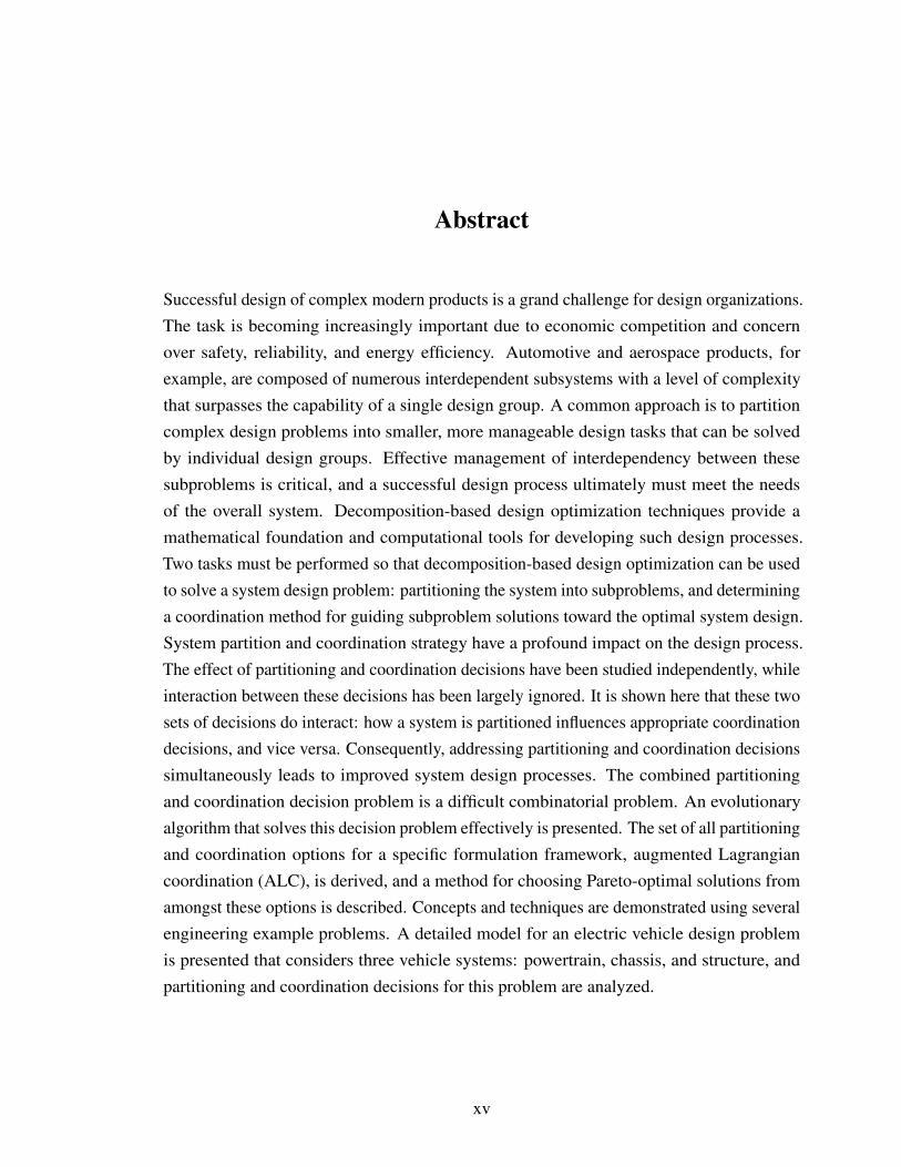
Successful design of complex modern products is a grand challenge for design organizations.The task is becoming increasingly important due to economic competition and concernover safety, reliability, and energy efficiency. Automotive and aerospace products, forexample, are composed of numerous interdependent subsystems with a level of complexitythat surpasses the capability of a single design group. A common approach is to partitioncomplex design problems into smaller, more manageable design tasks that can be solvedby individual design groups. Effective management of interdependency between thesesubproblems is critical, and a successful design process ultimately must meet the needsof the overall system. Decomposition-based design optimization techniques provide amathematical foundation and computational tools for developing such design processes.Two tasks must be performed so that decomposition-based design optimization can be usedto solve a system design problem: partitioning the system into subproblems, and determininga coordination method for guiding subproblem solutions toward the optimal system design.System partition and coordination strategy have a profound impact on the design process.The effect of partitioning and coordination decisions have been studied independently, whileinteraction between these decisions has been largely ignored. It is shown here that these twosets of decisions do interact: how a system is partitioned influences appropriate coordinationdecisions, and vice versa. Consequently, addressing partitioning and coordination decisionssimultaneously leads to improved system design processes. The combined partitioningand coordination decision problem is a difficult combinatorial problem. An evolutionaryalgorithm that solves this decision problem effectively is presented. The set of all partitioningand coordination options for a specific formulation framework, augmented Lagrangiancoordination (ALC), is derived, and a method for choosing Pareto-optimal solutions fromamongst these options is described. Concepts and techniques are demonstrated using severalengineering example problems. A detailed model for an electric vehicle design problemis presented that considers three vehicle systems: powertrain, chassis, and structure, andpartitioning and coordination decisions for this problem are analyzed.
xv

Chapter 1
Decomposition-based Design Optimization
Many products designed by engineers are too complex to be addressed by a single designer oreven a single design group. Examples of products that are complex systems include aircraft,automobiles, and electronics. A common approach for addressing challenges associatedwith complex system design is to divide the product design task into smaller and moremanageable design problems. For example, separate groups involved in automotive designmay each be working on different vehicle systems, such as powertrain, frame, or chassisdesign. A primary challenge in this approach arises from interactions between the smallerdesign problems. These subproblems cannot be solved in complete isolation from each other.Decisions in one subproblem affect what decisions should be made in other subproblems. Itis essential to coordinate subproblem solution such that the resulting subsystem designs areconsistent with each other, and so that the subsystem designs together comprise an overalldesign that is optimal for the entire system, not just optimal for individual parts.
A decomposition-based approach to engineering system design requires considerableforethought before design activities can commence. Not all ways of dividing, or partitioning,a system are equal. Some partitions will enhance the effectiveness of the design process. Inaddition, the strategy for coordinating subproblems has significant influence over designprocess success. An appropriate system partition and an effective coordination strategy mustbe developed before the design process is launched. Choice of partition and coordinationstrategy should be considered together. The form of a system partition will influence howthe subproblems are most effectively coordinated, and the intended coordination strategywill affect partitioning decisions. This dissertation addresses how to make partitioning andcoordination decisions that lead to less complex and more effective decomposed designprocesses.
Computer-aided engineering (CAE) tools have reached the level of sophistication re-quired for widespread use in engineering design. Engineering products can be designedand prototyped in a virtual environment, and then tested using computer simulations. Math-ematical optimization techniques can be used to vary product design variables and test
1
virtual prototypes in search of designs that are optimal with respect to some criteria; opti-mization algorithms can reduce the number of virtual tests required to identify an optimaldesign. Application of CAE and optimization algorithms reduces the need for costly physicalprototypes and expedites product development.
Complicated products can also be simulated successfully using CAE and designed usingoptimization algorithms. Often this involves the use of several separate, but interacting, CAEtools. The complexity of the simulations and the difficulty of the associated optimizationproblem can present a significant challenge. Many times a single optimization algorithmcannot manage the design of the system because of the large number of design variablesor constraints, or because of the complex nature of the system. As with the human-baseddesign process, a simulation-based design process can also be partitioned into smaller andeasier to solve subproblems. Interactions exist between subproblems, requiring some typeof coordination strategy to guide repeated subproblem solutions toward a consistent stateand a design that is optimal for the entire system. Numerous methods have been developedto solve simulation-based design problems in this manner. We refer to this approach asdecomposition-based design optimization.
Application of decomposition-based design optimization to a simulation-based systemdesign problem also requires the a priori definition of a system partition and coordinationstrategy. The relationships between partitioning and coordination decisions are studied here.The results provide a deeper understanding into effective application of decomposition-baseddesign optimization, aiding system designers in refining simulation-based design processes.Techniques for making optimal partitioning and coordination decisions, specifically forsimulation-based design, are introduced here. Application of these techniques can furtherreduce product development time and cost when simulation-based design is a significantcomponent of a product development process.
This chapter provides an overview of engineering system design and the use of mathe-matical optimization for engineering design. An overview of decomposition-based designoptimization is then provided, followed by an example design problem that illustrates theimpact of partitioning and coordination decisions on system design.
1.1 Engineering System Design
Complex systems are composed of several interacting members. Overall system behavioris not the simple sum or collection of constituent member behavior, but is somethingdistinct that emerges from intricate member interrelationships. Analysis and design ofcomplex systems requires something more than a dissociated approach; interactions must be
2
acknowledged, studied, and exploited to extract superior results.Many modern engineered products are congruent with the above description of complex
systems. They are composed of numerous subsystems and components interrelated throughcomplex interactions. If each subsystem is designed independently, the resulting systemwill not reach its potential; it may not even work. Effects of system interactions can bediscovered empirically, but this is an expensive and slow process. Formal techniques thatexplicitly manage interactions can enhance the system design process.
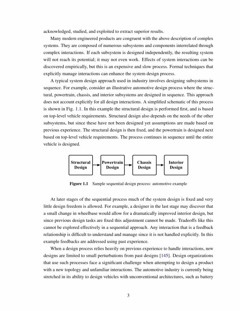
A typical system design approach used in industry involves designing subsystems insequence. For example, consider an illustrative automotive design process where the struc-tural, powertrain, chassis, and interior subsystems are designed in sequence. This approachdoes not account explicitly for all design interactions. A simplified schematic of this processis shown in Fig. 1.1. In this example the structural design is performed first, and is basedon top-level vehicle requirements. Structural design also depends on the needs of the othersubsystems, but since these have not been designed yet assumptions are made based onprevious experience. The structural design is then fixed, and the powertrain is designed nextbased on top-level vehicle requirements. The process continues in sequence until the entirevehicle is designed.
Structural Design
Powertrain Design
Chassis Design
Interior Design
Figure 1.1 Sample sequential design process: automotive example
At later stages of the sequential process much of the system design is fixed and verylittle design freedom is allowed. For example, a designer in the last stage may discover thata small change in wheelbase would allow for a dramatically improved interior design, butsince previous design tasks are fixed this adjustment cannot be made. Tradeoffs like thiscannot be explored effectively in a sequential approach. Any interaction that is a feedbackrelationship is difficult to understand and manage since it is not handled explicitly. In thisexample feedbacks are addressed using past experience.
When a design process relies heavily on previous experience to handle interactions, newdesigns are limited to small perturbations from past designs [145]. Design organizationsthat use such processes face a significant challenge when attempting to design a productwith a new topology and unfamiliar interactions. The automotive industry is currently beingstretched in its ability to design vehicles with unconventional architectures, such as battery
3

electric (BEV) and hybrid electric (HEV) vehicles. Vehicle subsystems behave and interactin sometimes unexpected ways. Engineers can no longer rely on experience and intuitionto resolve all difficulties that arise due to system interactions. Market pressure demandssolutions before resolution can be obtained through experience. More sophisticated systemdesign processes can help tackle this evolving problem.
The sequential process described above can be regarded as a single iteration of the blockcoordinate descent (BCD) algorithm [20]. The process could be iterated in an effort toaddress feedback interactions and generate an optimal system design, but the number ofiterations required may exceed available time or resources. A more effective technique thataddresses the needs of system design specifically is required. BCD does not retain enoughdesign freedom in later stages, and design decisions do not account explicitly for effects onthe complete system. Design freedom should be extended further into the process, and morecomplete system knowledge needs to be available and used earlier in the process [55].
1.2 Design Optimization
Mathematical optimization techniques are useful when quantitative decisions are to be madebased on criteria that can be expressed using a mathematical model. These techniques havebeen applied for decades to operations research problems such as supply chain, scheduling,or network problems [22]. More recently, optimization has been established as a tool forengineering design [110]. This section reviews briefly fundamentals of optimization, andthen discusses how to apply optimization to engineering design.
Mathematical optimization techniques seek to find the minimum of a function of n
variables without evaluating all possible variable values. The function to be minimized isthe objective function f (x), and the variables it depends on are represented by the vector x.All vectors in this dissertation are assumed to be row vectors unless otherwise noted. Thevariables can be real-valued (x ∈ Rn) or discrete; discrete variables may be integer (x ∈ Zn),binary (x ∈ 0,1n), or categorical (e.g., x ∈ steel,aluminum,carbon fiber composite).Constrained optimization problems have limits on the values design variables may assume.Equality constraints require that design variables satisfy a relation exactly, while inequal-ity constraints place bounds on values that design variables can assume. A constrainedoptimization problem in negative null form is stated as:
4
minx
f (x)
subject to g(x)≤ 0 (1.1)h(x) = 0,
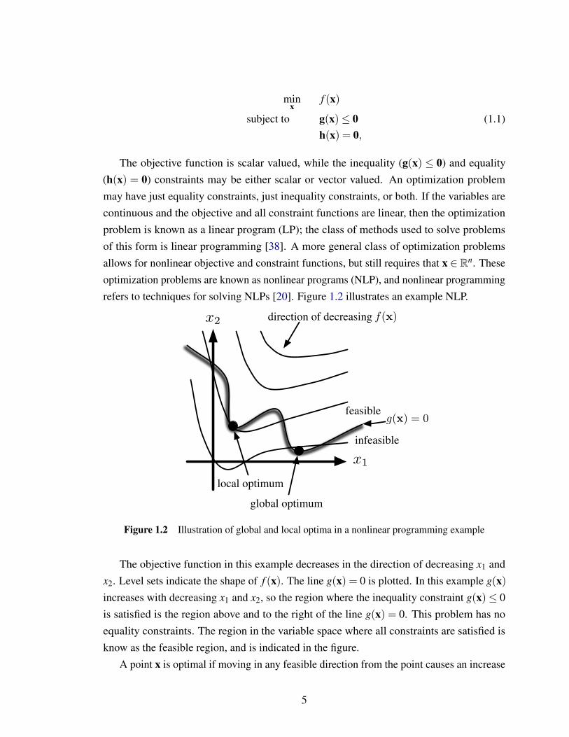
The objective function is scalar valued, while the inequality (g(x) ≤ 0) and equality(h(x) = 0) constraints may be either scalar or vector valued. An optimization problemmay have just equality constraints, just inequality constraints, or both. If the variables arecontinuous and the objective and all constraint functions are linear, then the optimizationproblem is known as a linear program (LP); the class of methods used to solve problemsof this form is linear programming [38]. A more general class of optimization problemsallows for nonlinear objective and constraint functions, but still requires that x ∈ Rn. Theseoptimization problems are known as nonlinear programs (NLP), and nonlinear programmingrefers to techniques for solving NLPs [20]. Figure 1.2 illustrates an example NLP.
x1
x2
infeasible
feasible
direction of decreasing f(x)
global optimum
local optimum
g(x) = 0
Figure 1.2 Illustration of global and local optima in a nonlinear programming example
The objective function in this example decreases in the direction of decreasing x1 andx2. Level sets indicate the shape of f (x). The line g(x) = 0 is plotted. In this example g(x)increases with decreasing x1 and x2, so the region where the inequality constraint g(x)≤ 0is satisfied is the region above and to the right of the line g(x) = 0. This problem has noequality constraints. The region in the variable space where all constraints are satisfied isknow as the feasible region, and is indicated in the figure.
A point x is optimal if moving in any feasible direction from the point causes an increase
5
in the objective function value. The symbol x∗ denotes an optimal variable vector. If X isthe set of all feasible points, a direction s ∈Rn is feasible if there exists a scalar αu > 0 suchthat x+αs ∈X for all 0≤ α ≤ αu. The example in Fig. 1.2 has two constrained optima.In each case the inequality constraint is active. A constraint is active if its removal changesthe location of x∗. Active inequality constraints are satisfied with equality. If a problem hasmultiple optima, the optimum with the lowest value is the global optimum. All others arelocal optima. A constrained NLP may have an unconstrained optimum if there exists a pointin the interior of X where all possible directions s lead to increased f (x).
The preceding paragraph informally describes optimality conditions for NLPs. In somecases optimality conditions can be used to derive a system of equations that can be usedto solve for x∗ directly. Monotonicity analysis (MA) is another solution approach thatexploits knowledge of monotonicity in objective and constraint functions to identify activeconstraints [110]. If MA cannot be used to completely solve a problem, it can possibly helpreduce its complexity and provide helpful insights. If direct solution or solution throughMA is not possible, an iterative algorithm for NLPs may be employed. Most are basedon objective and constraint function gradients. Gradient-based algorithms can be appliedonly when functions are continuous and smooth. If a problem is also convex1 a gradient-based algorithm will identify the global optimum, but without convexity these algorithmswill find only local optima. Examples of successful gradient-based algorithms for NLPsinclude the generalized reduced gradient (GRG) method [91] and sequential quadraticprogramming (SQP) [69, 111]. Much of the development in subsequent chapters assumesthat the optimization problems under consideration can be solved using a gradient-basedalgorithm.
Gradient-based algorithms are normally computationally efficient, i.e., they convergequickly and require relatively few function evaluations when compared to gradient-free meth-ods. Unfortunately, gradient-based methods can fail when functions are non-differentiableor numerically noisy. They typically do not handle problems with discrete variables, andcan perform inconsistently when applied to ill-conditioned problems. Several gradient freemethods have been developed as alternatives. Evolutionary algorithms (EAs) use principlesof natural selection to gradually improve the quality of a population of candidate solutionsover several generations [49, 73]. Simulated annealing (SA) is another heuristic algorithm;it considers single design points (rather than a population) and uses a stochastic searchtechnique with a positive probability of selecting worse points to aid escaping local optima[81]. This algorithm’s name comes from the ‘cooling schedule’ that guides the probabilityof selecting an inferior point during the search. Another class of stochastic search algo-
1A problem is convex if f (x) is a convex function and if X is a convex set.
6
rithms selects random points around a candidate solution to evaluate and determine a newcandidate solution point [130]. As with SAs, these algorithms are not population-based. Thedistribution of search points is influenced by information obtained during the optimizationprocess.
Heuristic methods such as EAs and SAs are not based on optimality conditions, so cannotguarantee that the solution obtained is an optimum. They can offer good approximationsto the optimum for problems that cannot be solved with gradient-based methods. Anotherdisadvantage of these methods is the large number of function evaluations that typically arerequired. An alternative exists that is based on optimality conditions involving subgradients,which are in essence a type of gradient for non-smooth functions defined in Clarke’s calculus[32]. This alternative method is mesh adaptive direct search (MADS), and is positionedin the spectrum of optimization methods between gradient-based methods and heuristicmethods [14]. MADS can handle non-smooth problems, but normally does not require asmany function evaluations as EAs or SAs.
Engineering design problems can be posed naturally as constrained optimization prob-lems. Normally at least one metric is readily identified as an objective function, such assome key performance metric. Engineering design problems are full of design requirementsthat can be expressed as constraints (e.g., stress, deflection, packaging, temperature, orvibration requirements). Constraints based on design requirements are termed design con-straints. Objective and constraint functions can be calculated using analytical expressionsor computer simulations. The inputs to these expressions or simulations are quantities thatparametrically characterize the design of a product, such as physical geometry. A subset ofthese quantities is chosen as the set of design variables, x. Design variables are allowed tovary in the design problem, while the remaining function inputs, termed design parameters,are held fixed when solving a design optimization problem. In summary, in engineeringdesign optimization we seek to optimize the performance of a product subject to designconstraints, with respect to design variables.
In some system optimization formulations the optimization algorithm selects valuesfor quantities that are not design variables. To avoid confusion in terminology, we definedecision variables to be any quantity that are variables in the design optimization problem.The set of decisions variables includes design variables and possibly other quantities.
Design optimization is a logical extension to CAE software. Tremendous effort has beendevoted to development of accurate and efficient software for engineering analysis. Thesesoftware can be used to analyze existing prototypes or products, or used as tools to testdesign alternatives proposed by engineers before fabrication. Engineers can also use CAEsoftware to test manually adjusted design variables. This process can help build intuition
7
for a product, and can be a good approach when only a few design variables are used, butbecomes unwieldy as the number of design variables increases. While manual search maybe impractical in many cases, optimization algorithms can trace an efficient path toward theoptimal design. A design optimization approach requires fewer function evaluations andleads to a superior design.
The effectiveness of design optimization depends on our ability to model accuratelyactual product behavior. The solution to a design optimization problem does not generatethe optimal design for the real product, but the optimal design for a virtual product asrepresented by a mathematical model. CAE tools are becoming more mature and offerincreasing levels of modeling accuracy, and have been a factor in the success of designoptimization as a practical engineering tool.
1.3 Decomposition-based Design Optimization
Applying design optimization techniques to engineering system design presents additionalchallenges. As with general engineering system design, approaching the design of a systemas a single entity may be impractical. A single optimization algorithm may not be capable ofhandling the demands of designing an entire system. The system optimization problem canbe partitioned into smaller subproblems, each solved separately. The subproblems are linkedthrough common design variables and analysis interactions. Subproblems must be solved ina way that leads to a system design that accounts for these links, and is optimal for the entiresystem. The task of guiding subproblem solutions toward an optimal system design is calledcoordination. This approach to engineering system design is known as decomposition-baseddesign optimization.
A broad class of methods for decomposition-based design optimization, known asmultidisciplinary design optimization (MDO), has been developed to address industry needsfor engineering system design. Most have been developed for situations where severalengineering analyses must be integrated for designing a single component or product, whereeach analysis pertains to a different aspect of the same component. Aeroelastic design is astandard example of an MDO application. Suppose an airplane wing is to be designed, givingheed to both structural and aerodynamic considerations. If the wing is sufficiently stiff, wecan assume that the wing does not deform much when subject to aerodynamic pressure. Thisallows us to use the undeformed wing shape when conducting the aerodynamic analysis,making the aerodynamic analysis independent of the structural analysis. If the wing is notsufficiently stiff for this assumption to hold, the aerodynamic analysis should be based onthe deformed wing shape as computed by the structural analysis. The structural analysis in
8
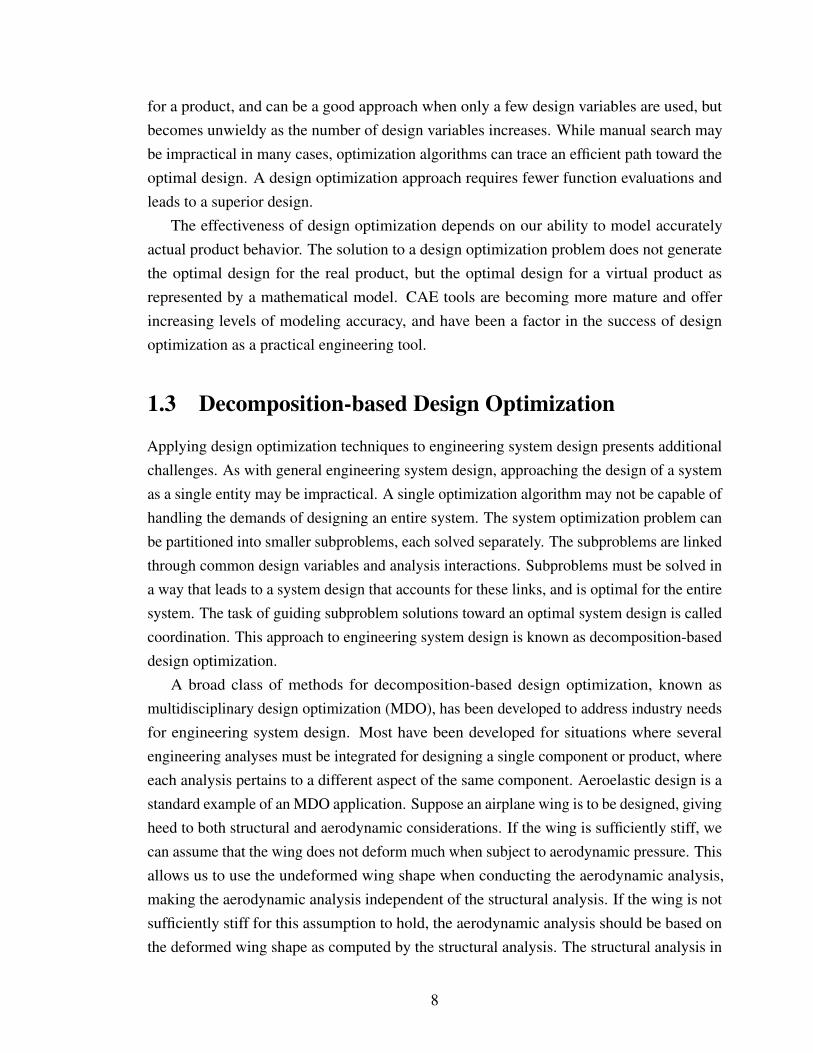
turn requires the aerodynamic pressure distribution over the wing surface to compute thedeformed shape. The two analyses are coupled, as depicted in Fig. 1.3.
Aerodynamic Analysis
Structural Analysis
deformedshape
pressure distribution
Figure 1.3 Aeroelastic analysis
Iterative techniques are required to find a state of pressure and deformation such that theanalyses are consistent with each other. The task of solving coupled analyses simultaneouslyis known as multidisciplinary analysis (MDA). Multiphysics software has been developed toaddress specific types of MDA.
The presence of analysis coupling complicates system design. Many MDO methodsare designed to manage this type of coupling. Cramer et al. identified several importantMDO formulations [35], and Sobieski and Haftka provided an extensive review of earlyMDO methods [128]. Industry needs motivating MDO development are summarized in [55]and [61]. Common points include the need to compress design cycle time, improve productquality, increase design flexibility, and more competently characterize, manage, and exploitsystem interactions. Chapter 4 introduces and demonstrates several important methods fordecomposition-based design optimization. These methods are more broadly applicable thanto just systems partitioned by discipline; partitions may be along disciplinary, physical,process boundaries, or some combination thereof.
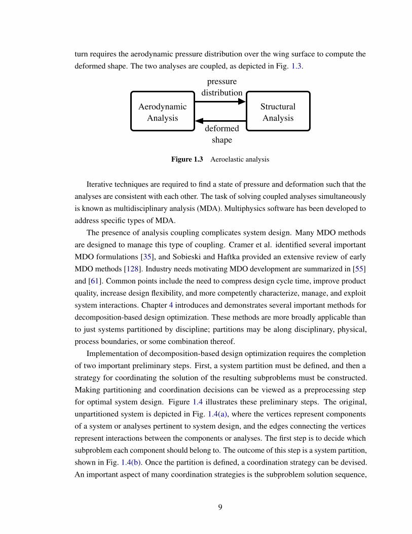
Implementation of decomposition-based design optimization requires the completionof two important preliminary steps. First, a system partition must be defined, and then astrategy for coordinating the solution of the resulting subproblems must be constructed.Making partitioning and coordination decisions can be viewed as a preprocessing stepfor optimal system design. Figure 1.4 illustrates these preliminary steps. The original,unpartitioned system is depicted in Fig. 1.4(a), where the vertices represent componentsof a system or analyses pertinent to system design, and the edges connecting the verticesrepresent interactions between the components or analyses. The first step is to decide whichsubproblem each component should belong to. The outcome of this step is a system partition,shown in Fig. 1.4(b). Once the partition is defined, a coordination strategy can be devised.An important aspect of many coordination strategies is the subproblem solution sequence,
9
illustrated in Fig. 1.4(c).
(a) Unpartitioned system (b) System partitioned into sub-problems
(c) Subproblem coordinationstrategy
Figure 1.4 Process for implementing decomposition-based design optimization
While the focus here is on simulation-based design, an organizational analogy is in-structive. Suppose the vertices in Fig. 1.4(a) represent positions or tasks within a designorganization. Before a large organization can embark on product design, it needs struc-ture [36]. First it is partitioned into groups. These groups can be formed according todiscipline, project, or hybrid divisions. Interaction must occur both within and betweengroups. Patterns of interaction along with an organizational partition define organizationalstructure. Interaction patterns, analogous to coordination, can take several different forms.Bureaucratic organizations are structured into a hierarchy, which can be orderly and efficientin certain cases. Horizontal organizations are non-hierarchic; these can be more adaptableto changes than hierarchic organizations.
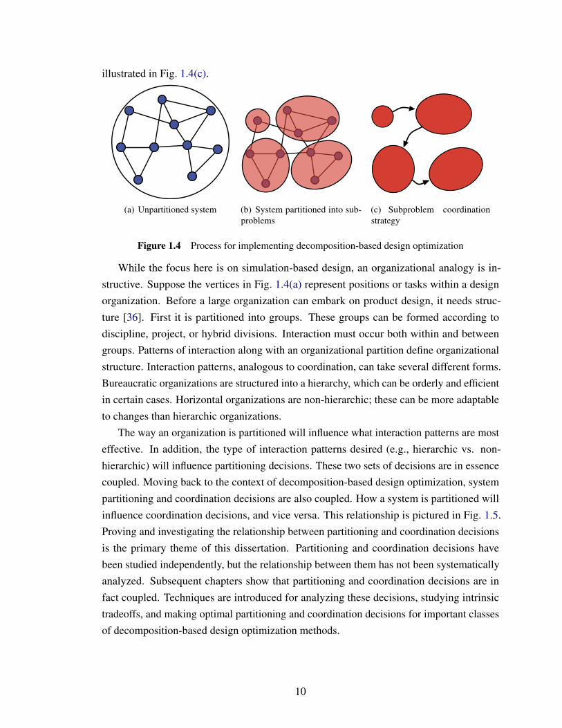
The way an organization is partitioned will influence what interaction patterns are mosteffective. In addition, the type of interaction patterns desired (e.g., hierarchic vs. non-hierarchic) will influence partitioning decisions. These two sets of decisions are in essencecoupled. Moving back to the context of decomposition-based design optimization, systempartitioning and coordination decisions are also coupled. How a system is partitioned willinfluence coordination decisions, and vice versa. This relationship is pictured in Fig. 1.5.Proving and investigating the relationship between partitioning and coordination decisionsis the primary theme of this dissertation. Partitioning and coordination decisions havebeen studied independently, but the relationship between them has not been systematicallyanalyzed. Subsequent chapters show that partitioning and coordination decisions are infact coupled. Techniques are introduced for analyzing these decisions, studying intrinsictradeoffs, and making optimal partitioning and coordination decisions for important classesof decomposition-based design optimization methods.
10
PartitioningDecisions
CoordinationDecisions
Figure 1.5 Dissertation hypothesis: Existence of coupling between partitioning and coordinationdecisions
1.4 Introductory Example
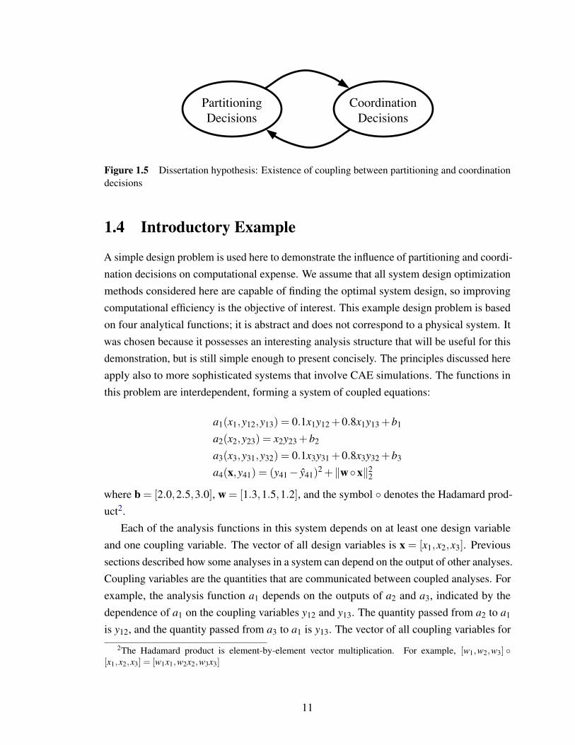
A simple design problem is used here to demonstrate the influence of partitioning and coordi-nation decisions on computational expense. We assume that all system design optimizationmethods considered here are capable of finding the optimal system design, so improvingcomputational efficiency is the objective of interest. This example design problem is basedon four analytical functions; it is abstract and does not correspond to a physical system. Itwas chosen because it possesses an interesting analysis structure that will be useful for thisdemonstration, but is still simple enough to present concisely. The principles discussed hereapply also to more sophisticated systems that involve CAE simulations. The functions inthis problem are interdependent, forming a system of coupled equations:
a1(x1,y12,y13) = 0.1x1y12 +0.8x1y13 +b1
a2(x2,y23) = x2y23 +b2
a3(x3,y31,y32) = 0.1x3y31 +0.8x3y32 +b3
a4(x,y41) = (y41− y41)2 +‖wx‖22
where b = [2.0,2.5,3.0], w = [1.3,1.5,1.2], and the symbol denotes the Hadamard prod-uct2.
Each of the analysis functions in this system depends on at least one design variableand one coupling variable. The vector of all design variables is x = [x1,x2,x3]. Previoussections described how some analyses in a system can depend on the output of other analyses.Coupling variables are the quantities that are communicated between coupled analyses. Forexample, the analysis function a1 depends on the outputs of a2 and a3, indicated by thedependence of a1 on the coupling variables y12 and y13. The quantity passed from a2 to a1
is y12, and the quantity passed from a3 to a1 is y13. The vector of all coupling variables for
2The Hadamard product is element-by-element vector multiplication. For example, [w1,w2,w3] [x1,x2,x3] = [w1x1,w2x2,w3x3]
11
the example system is y = [y12,y13,y23,y31,y32,y41]. In general, the coupling variable yi j isthe quantity passed from analysis function j to analysis function i. Although some couplingvariables in this system represent the same quantity, many decomposition-based designoptimization methods utilize multiple coupling variable copies. This requires an explicitdistinction between all coupling variables. Coupling variable and other system optimizationnotation will be defined more precisely in the following chapter.
The design problem based on the four analysis functions described above is an uncon-strained minimization problem in three variables:
minx=[x1,x2,x3]
a4(x,y41) (1.2)
The optimization algorithm will choose iteratively new values for x as it seeks a minimumvalue for a4. Since a4 directly or indirectly depends on all design and coupling variables, allfour analysis functions must be evaluated for the value of x provided by the optimizationalgorithm at each iteration. Observe that this system possesses circular dependence betweenfunctions, also called feedback coupling. For example, a1 depends on the output of a2,which depends on the output of a3, which depends on the output of a1. Therefore, a1 cannotbe computed using a sequential evaluation technique; an iterative scheme is required. Acommon approach, known as fixed point iteration (FPI), starts with a guess for unknowncoupling variable values, evaluates the analysis functions in sequence, updates the initialguesses, and repeats until coupling variable values converge to a ‘fixed point’ [28]. Atconvergence the system is said to have coupling variable consistency. FPI does not alwaysconverge, and should be used with caution [6]. Coupling variable consistency is discussedin Section 2.1, and FPI convergence is addressed in Section 4.1.
Solution to Problem 1.2 implicitly requires a nested approach where an analysis al-gorithm, such as FPI, must be used to find a consistent set of coupling variables at everyoptimization iteration because of feedback coupling. In other words, the optimization prob-lem is an outer loop process that seeks to find an optimal design vector, while the analysisalgorithm is an inner loop process that seeks to find a consistent coupling variable vectorfor every design vector considered along the way. The computational expense added by theinner loop process can be considerable, and steps should be taken to minimize it. Analysisfeedback coupling can be difficult to handle, but is present in many important engineeringdesign problems. This dissertation discusses several techniques for understanding andmanaging analysis feedback coupling in system design optimization.
12
1.4.1 Coordination Decisions
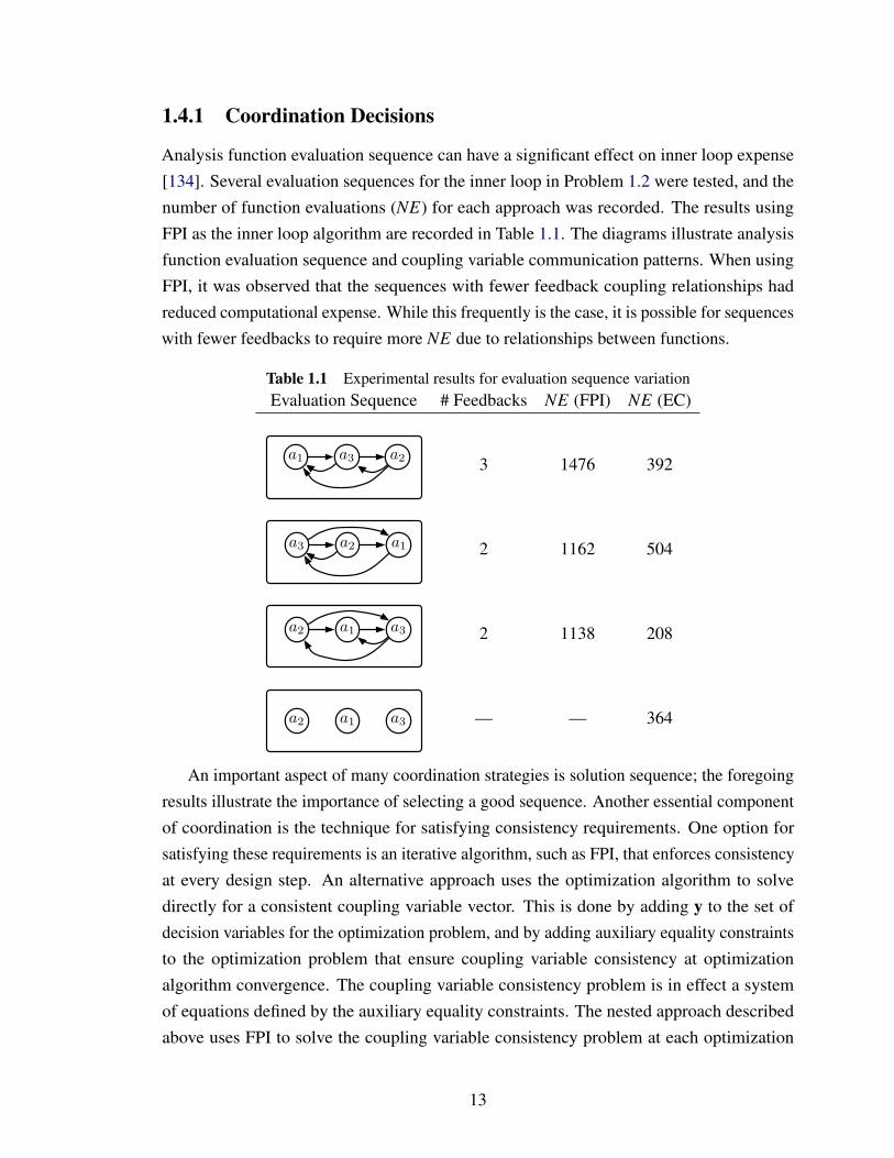
Analysis function evaluation sequence can have a significant effect on inner loop expense[134]. Several evaluation sequences for the inner loop in Problem 1.2 were tested, and thenumber of function evaluations (NE) for each approach was recorded. The results usingFPI as the inner loop algorithm are recorded in Table 1.1. The diagrams illustrate analysisfunction evaluation sequence and coupling variable communication patterns. When usingFPI, it was observed that the sequences with fewer feedback coupling relationships hadreduced computational expense. While this frequently is the case, it is possible for sequenceswith fewer feedbacks to require more NE due to relationships between functions.
Table 1.1 Experimental results for evaluation sequence variationEvaluation Sequence # Feedbacks NE (FPI) NE (EC)
a1 a3 a2 3 1476 392
a1a3 a2 2 1162 504
a1 a3a2 2 1138 208
a1 a3a2 — — 364
An important aspect of many coordination strategies is solution sequence; the foregoingresults illustrate the importance of selecting a good sequence. Another essential componentof coordination is the technique for satisfying consistency requirements. One option forsatisfying these requirements is an iterative algorithm, such as FPI, that enforces consistencyat every design step. An alternative approach uses the optimization algorithm to solvedirectly for a consistent coupling variable vector. This is done by adding y to the set ofdecision variables for the optimization problem, and by adding auxiliary equality constraintsto the optimization problem that ensure coupling variable consistency at optimizationalgorithm convergence. The coupling variable consistency problem is in effect a systemof equations defined by the auxiliary equality constraints. The nested approach describedabove uses FPI to solve the coupling variable consistency problem at each optimization
13
iteration. The auxiliary equality constraint approach uses the optimization algorithm to solvethe coupling variable consistency problem in tandem with the optimization problem, whichcan provide a computational advantage in some cases. The formulation for the exampleproblem using this equality constraint approach is:
minx,y
a4(x,y41)
subject to y12−a2(x2,y23) = 0y13−a3(x3,y31,y32) = 0y23−a3(x3,y31,y32) = 0 (1.3)y31−a1(x1,y12,y13) = 0y32−a2(x2,y23) = 0y41−a1(x1,y12,y13) = 0
The fourth row of Table 1.1 corresponds to the solution approach defined in Problem1.3. In this example a substantial computational benefit is realized. A hybrid coordinationstrategy exists that incorporates aspects of the nested approach and the equality constraintapproach. Balling and Sobieski suggested another alternative approach where the analysisfunctions are solved once in sequence, and auxiliary equality constraints are used to handlefeedback coupling relationships only, rather than all coupling relationships [15]. Thistechnique was used to solve the example problem using the three sequences listed in Table1.1, and the results are given in the last column. Using the first sequence, we have threefeedback relationships to satisfy using equality constraints. The design formulation is:
minx,y12,y13,y32
a4(x,y41)
subject to y12−a2(x2,y23) = 0 (1.4)y13−a3(x3,y31,y32) = 0y32−a2(x2,y23) = 0
Consistency for the feedback coupling variables y12, y13, and y32 is satisfied via op-timization equality constraints, and consistency for y23, y31, and y41 is satisfied throughanalysis function sequencing. The second sequence option has two feedback relationshipsto satisfy:
14
minx,y31,y32
a4(x,y41)
subject to y31−a1(x1,y12,y13) = 0 (1.5)y32−a2(x2,y23) = 0
The third sequence has two feedback couplings, and the corresponding formulation is:
minx,y13,y23
a4(x,y41)
subject to y13−a3(x3,y31,y32) = 0 (1.6)y23−a3(x3,y31,y32) = 0
This last approach proved to be most efficient out of all seven coordination optionspresented, requiring only 208 function evaluations. This is an 86% reduction from the firstoption, showing the importance of making proper coordination decisions. The effect ofpartitioning decisions on this example problem will now be explored.
1.4.2 Partitioning Decisions
Analysis functions may be grouped together to form blocks of a system partition. Indistributed optimization an optimization problem is defined for each of these blocks. Whena single optimization problem is employed, these blocks can be used to divide up systemanalysis. Two approaches are considered here. In both approaches FPI is employed withineach block to achieve coupling variable consistency between functions inside a block. Inthe first approach FPI is also used to satisfy coupling variable consistency for relationshipsbetween blocks. In the second approach auxiliary equality constraints enforce consistencybetween blocks. The results are summarized in Table 1.2.
The first approach exhibited a dramatic increase in function evaluations for every par-tition. The number of evaluations is multiplied because there exist three levels of nestingin the solution approach. No significant difference exists between partitions for the firstapproach in this example problem. The second and third partitions required the exact samenumber of function evaluations; in this case swapping the order of analysis blocks has noimpact on solution expense. The second approach applied to the second partition requiredonly 366 function evaluations. While this is not the lowest number observed, the resultis significant because the same a1→ a3→ a2 sequence required 392 evaluations with theunpartitioned auxiliary equality constraint approach. This shows that synergy exists betweenpartitioning and coordination decisions for this example. Subsequent chapters develop a
15
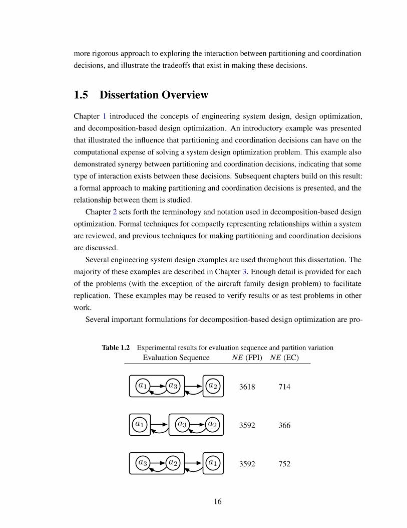
more rigorous approach to exploring the interaction between partitioning and coordinationdecisions, and illustrate the tradeoffs that exist in making these decisions.
1.5 Dissertation Overview
Chapter 1 introduced the concepts of engineering system design, design optimization,and decomposition-based design optimization. An introductory example was presentedthat illustrated the influence that partitioning and coordination decisions can have on thecomputational expense of solving a system design optimization problem. This example alsodemonstrated synergy between partitioning and coordination decisions, indicating that sometype of interaction exists between these decisions. Subsequent chapters build on this result:a formal approach to making partitioning and coordination decisions is presented, and therelationship between them is studied.
Chapter 2 sets forth the terminology and notation used in decomposition-based designoptimization. Formal techniques for compactly representing relationships within a systemare reviewed, and previous techniques for making partitioning and coordination decisionsare discussed.
Several engineering system design examples are used throughout this dissertation. Themajority of these examples are described in Chapter 3. Enough detail is provided for eachof the problems (with the exception of the aircraft family design problem) to facilitatereplication. These examples may be reused to verify results or as test problems in otherwork.
Several important formulations for decomposition-based design optimization are pro-
Table 1.2 Experimental results for evaluation sequence and partition variationEvaluation Sequence NE (FPI) NE (EC)
a1 a3 a2 3618 714
a1 a3 a2 3592 366
a1a3 a2 3592 752
16
vided in Chapter 4. Examples are used to elucidate application of these formulations and toreveal properties relevant to partitioning and coordination decisions. Particular attention ispaid to a class of formulations that is used in later chapters as the basis for partitioning andcoordination decisions. Algorithms in this class have proven convergence properties andhave the flexibility required to adapt to a wide range of problem structures.
Partitioning and coordination decisions for decomposition-based design optimizationare formalized in Chapter 5. These decisions are shown to be coupled for three examplesystems. A technique is introduced for analyzing the tradeoff between coordination andsubproblem solution expense. This analysis aids system designers in determining whether adecomposition-based approach should be used, and if so, what partitioning and coordinationdecisions may lead to reduced solution complexity. The techniques in Chapter 5 utilizeexhaustive enumeration of partitioning and coordination options. While effective for smallsystems, exhaustive enumeration is impractical for use in analyzing larger systems. Anevolutionary algorithm is presented in Chapter 6 that solves the optimal partitioning andcoordination decision problem for larger systems. The evolutionary algorithm is applied tothe three small example systems from Chapter 5, and its results are compared to the exactsolutions obtained with exhaustive enumeration. The evolutionary algorithm is then appliedto a structural design problem that is too large for exhaustive enumeration.
Coordination decisions addressed through Chapter 6 are limited to subproblem sequence.Another aspect of coordination decisions is how to structure the links between subproblems.This is addressed in Chapter 7 for a specific formulation called augmented Lagrangian coor-dination (ALC). A new class of parallel ALC implementations is introduced. ALC providestremendous flexibility in linking structure, but manually determining an appropriate linkingstructure can be overwhelming due to the large number of possibilities. The techniquesintroduced in Chapter 7 provide a way to create systematically a linking structure tailored tothe needs of a particular system, along with choosing a system partition and coordinationstrategy.
The examples used through Chapter 7 are of low to moderate complexity. A moreinvolved design example is presented in Chapter 8. The design of a battery electric vehicle isaddressed using decomposition-based design optimization. Several different vehicle systemsare considered, including powertrain, structure, and chassis design. The model accountsfor many important interactions, such as the influence of component sizing and location onvehicle dynamics. The optimal partitioning and coordination decision method presented inChapter 7 is applied to the electric vehicle design problem. The concepts and results aresummarized in Chapter 9. A systematic procedure is outlined for approaching partitioningand coordination decisions in system optimization and in other applications.
17
Chapter 2
Partitioning and Coordination Decisions
The preceding chapter introduced the concept of decomposition-based design optimizationfor engineering systems, and demonstrated that partitioning and coordination (P/C) decisionscan have great impact on solution difficulty. This chapter constructs notation and terminologyneeded for more precise and detailed treatment of system design optimization and P/Cdecisions, reviews existing techniques for making P/C decisions, and establishes that nostudies have addressed interaction between partitioning and coordination decisions or thepotential impact of this interaction.
2.1 Decomposition-based System Design
The system design problems considered here involve multidisciplinary, coupled analyseswhere input/output properties are assumed to be known precisely. For example, in simulation-based design, each quantity of interest in the design problem is computed using a computersimulation, such as finite element analysis or multi-body dynamics simulation software.Each simulation must be provided a specific set of inputs to compute its correspondingoutputs; this prescribes a definite information flow direction. Output quantities cannot berecast as inputs, and vice versa. This is contrast to equation-based design, where frequentlyone of several variables that appear in design equations can be selected as an output variable.Flexibility in the set of output quantities causes ambiguity in information flow. Exactknowledge of information flow in simulation-based design allows us to construct systemdesign approaches that exploit directionality to reduce solution complexity.
Each simulation in a system design problem can be viewed as a vector-valued analysisfunction; it computes one output vector for every unique set of inputs. Simulations (i.e.,analysis functions) frequently depend on outputs of other simulations in addition to designvariables. When circular dependence exists among analysis functions the system is saidto possess feedback coupling. Analysis function outputs can be design objectives, designconstraints, or intermediate quantities. Figure 2.1 illustrates the possible relationships
18
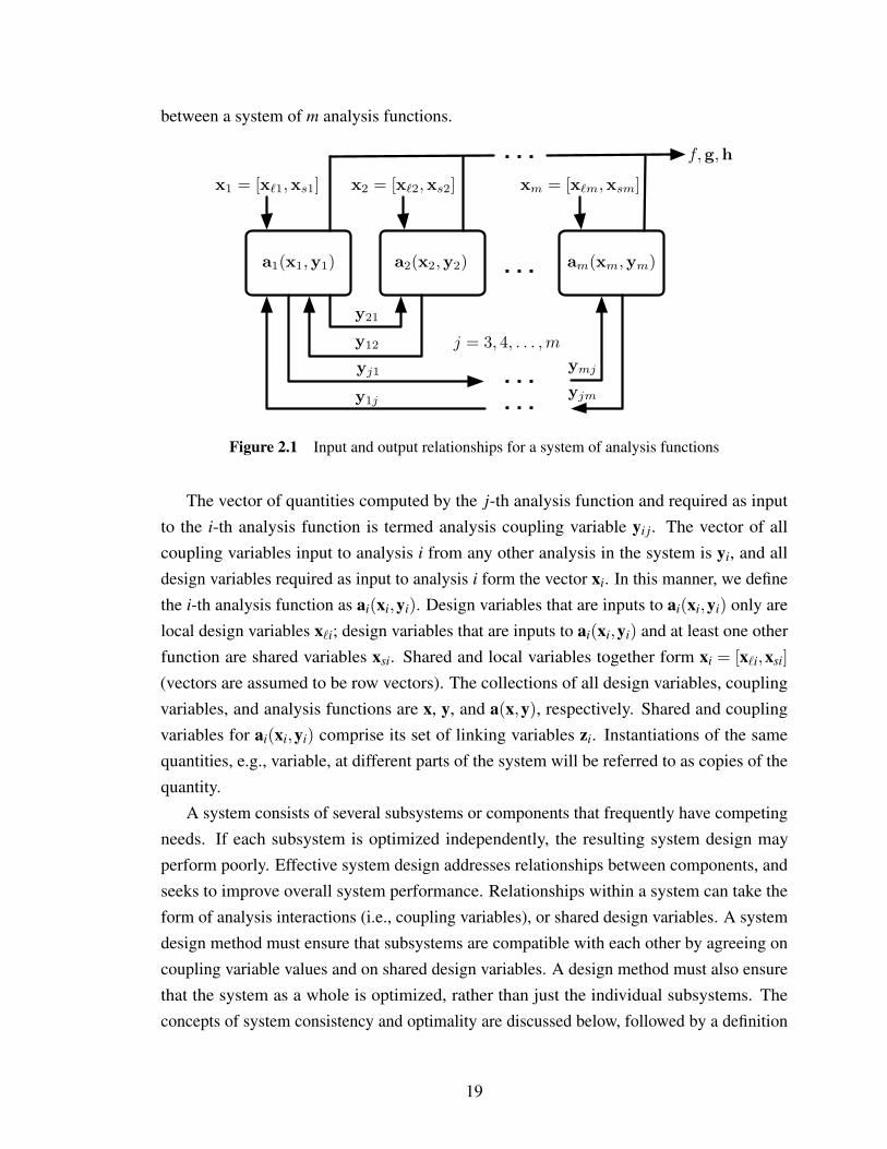
between a system of m analysis functions.
y21
y12
yj1
y1j
. . .
. . .
. . .
f,g,h. . .
a1(x1,y1) a2(x2,y2) am(xm,ym)
j = 3, 4, . . . ,m
ymj
yjm
xm = [x!m,xsm]x2 = [x!2,xs2]x1 = [x!1,xs1]
Figure 2.1 Input and output relationships for a system of analysis functions
The vector of quantities computed by the j-th analysis function and required as inputto the i-th analysis function is termed analysis coupling variable yi j. The vector of allcoupling variables input to analysis i from any other analysis in the system is yi, and alldesign variables required as input to analysis i form the vector xi. In this manner, we definethe i-th analysis function as ai(xi,yi). Design variables that are inputs to ai(xi,yi) only arelocal design variables x`i; design variables that are inputs to ai(xi,yi) and at least one otherfunction are shared variables xsi. Shared and local variables together form xi = [x`i,xsi](vectors are assumed to be row vectors). The collections of all design variables, couplingvariables, and analysis functions are x, y, and a(x,y), respectively. Shared and couplingvariables for ai(xi,yi) comprise its set of linking variables zi. Instantiations of the samequantities, e.g., variable, at different parts of the system will be referred to as copies of thequantity.
A system consists of several subsystems or components that frequently have competingneeds. If each subsystem is optimized independently, the resulting system design mayperform poorly. Effective system design addresses relationships between components, andseeks to improve overall system performance. Relationships within a system can take theform of analysis interactions (i.e., coupling variables), or shared design variables. A systemdesign method must ensure that subsystems are compatible with each other by agreeing oncoupling variable values and on shared design variables. A design method must also ensurethat the system as a whole is optimized, rather than just the individual subsystems. Theconcepts of system consistency and optimality are discussed below, followed by a definition
19
of distributed optimization.
2.1.1 System Consistency
A system is consistent if the values of all copies of a shared variable agree for all sharedvariables, and if the value of every coupling variable is equal to its corresponding analysisoutput. In other words, system consistency is achieved if shared variable and couplingvariable consistency requirements are met. It is essential that shared variable and couplingvariable consistency are managed separately to achieve the most efficient solution processesfor system design. System consistency is a necessary condition for system optimality.
Shared variable consistency is achieved if
x(k)q = x(l)
q ∀ k 6= l, k, l ∈ Ds(xq) (2.1)
is satisfied for all shared variables, where xq is a component of x that is shared among theanalysis functions ai(xi,yi) ∀i ∈ Ds(xq), with Ds(xq) being the set of indices of analysisfunctions that depend on the shared variable xq; superscripts indicate the analysis functionwhere the shared variable copy is input. A shared variable xq is consistent if the value for xq
input to every analysis function that depends on xq is identical.Coupling variable consistency is achieved, if for every coupling variable,
yi j−a j(x j,y j)Si j = 0 (2.2)
is satisfied, where the boolean matrix Si j selects the components of a j that correspondto yi j. The set of all such equality constraints is y− a(x,y)S = 0, where S is a selectionmatrix that extracts the components of a(x,y) that correspond to y. These coupling variableconsistency constraints are referred to as the system analysis equations. Equations (2.1) and(2.2) together form the system consistency constraints.
2.1.2 System Optimality
A system design optimization approach should ensure the resulting design is optimalwith respect to the system’s primary purpose. A single objective function that effectivelyrepresents this purpose should be selected. Section 1.1 described how design approachesthat do not consider all aspects of a system together may not identify designs that are systemoptimal. An effective design approach accounts for all system interactions, optimizes thesystem objective function, and ensures system consistency. The following formulation meets
20
these requirements:
minx
f (x,yp(x)) (2.3)
subject to g(x,yp(x))≤ 0
h(x,yp(x)) = 0,
where yp(x) is a solution to the system analysis equations for a given design, and theobjective and constraint function values are outputs of a subset of analysis functions. Thisformulation is known as multidisciplinary feasible (MDF) [35] or All-in-One (AiO), andimplicitly achieves shared variable consistency. For every optimization iterate x the systemanalysis equations must be solved for yp(x) to satisfy Eq. (2.2) for every coupling variable.This nested approach ensures both coupling variable and shared variable consistency, aswell as minimizes the system objective function f (x,yp(x)).
If no feedback loops exist among analysis functions, the system analysis equations can besatisfied simply by executing the analysis functions in the proper sequence; analysis functionoutputs provide the coupling variable values directly. An iterative algorithm is requiredfor system analysis if feedback loops exist. Alternatively, the optimization algorithm cansolve for yp(x) using equality constraints to enforce coupling variable consistency. Thisenables coarse-grained parallel processing and can ease numerical difficulties associatedwith strongly coupled analysis functions [6]. The Individual Disciplinary Feasible (IDF)formulation is the simplest way to use this approach [35]. Balling and Sobieski suggested ahybrid approach that uses function sequencing to satisfy feedforward coupling relationships,and equality constraints to satisfy feedback coupling relationships [15]. This hybrid approachwas demonstrated in Section 1.4.
2.1.3 Distributed Optimization
The two formulations for system optimization discussed above, MDF and IDF, are known assingle-level formulations because a single optimization algorithm is involved. Single-levelapproaches become unwieldy when the number of design variables or constraints is largeenough to approach optimization algorithm reliability or cost limits. Large systems canbe divided into several smaller optimization problems, called subproblems. Interactionsbetween subproblems must be managed such that the final result is consistent and optimalfor the entire system. This is accomplished through a coordination strategy that works withthe individual subproblems. This type of approach is known as multi-level or distributed
21
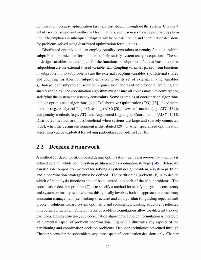
optimization, because optimization tasks are distributed throughout the system. Chapter 4details several single and multi-level formulations, and discusses their appropriate applica-tion. The emphasis in subsequent chapters will be on partitioning and coordination decisionsfor problems solved using distributed optimization formulations.
Distributed optimization can employ equality constraints or penalty functions withinsubproblem optimization formulations to help satisfy system analysis equations. The setof design variables that are inputs for the functions in subproblem i and at least one othersubproblem are the external shared variables xsi. Coupling variables passed from functionsin subproblem j to subproblem i are the external coupling variables yi j. External sharedand coupling variables for subproblem i comprise its set of external linking variableszi. Independent subproblem solution requires local copies of both external coupling andshared variables. The coordination algorithm must ensure all copies match at convergence,satisfying the system consistency constraints. Some examples of coordination algorithmsinclude optimization algorithms (e.g., Collaborative Optimization (CO) [25]), fixed pointiteration (e.g., Analytical Target Cascading (ATC) [80]), Newton’s method (e.g., ATC [139]),and penalty methods (e.g., ATC and Augmented Lagrangian Coordination (ALC) [141]).Distributed methods are most beneficial when systems are large and sparsely connected[128], when the design environment is distributed [29], or when specialized optimizationalgorithms can be exploited for solving particular subproblems [88, 105].
2.2 Decision Framework
A method for decomposition-based design optimization (i.e., a decomposition method) isdefined here to include both a system partition and a coordination strategy [145]. Before wecan use a decomposition method for solving a system design problem, a system partitionand a coordination strategy must be defined. The partitioning problem (P) is to decidewhich of m analysis functions should be clustered into each of the N subproblems. Thecoordination decision problem (C) is to specify a method for satisfying system consistencyand system optimality requirements; this typically involves both an approach to consistencyconstraint management (i.e., linking structure) and an algorithm for guiding repeated sub-problem solutions toward system optimality and consistency. Linking structure is reflectedin problem formulation. Different types of problem formulations allow for different types ofpartitions, linking structure, and coordination algorithms. Problem formulation is thereforean elemental aspect of problem coordination. Figure 2.2 illustrates key aspects of thepartitioning and coordination decision problems. Decision techniques presented throughChapter 6 consider the subproblem sequence aspect of coordination decisions only. Chapter
22
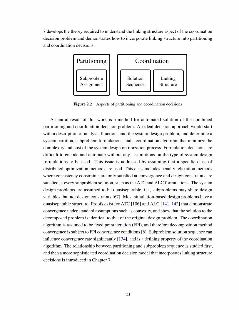
7 develops the theory required to understand the linking structure aspect of the coordinationdecision problem and demonstrates how to incorporate linking structure into partitioningand coordination decisions.
Partitioning Coordination
SubproblemAssignment
SolutionSequence
LinkingStructure
Figure 2.2 Aspects of partitioning and coordination decisions
A central result of this work is a method for automated solution of the combinedpartitioning and coordination decision problem. An ideal decision approach would startwith a description of analysis functions and the system design problem, and determine asystem partition, subproblem formulations, and a coordination algorithm that minimize thecomplexity and cost of the system design optimization process. Formulation decisions aredifficult to encode and automate without any assumptions on the type of system designformulations to be used. This issue is addressed by assuming that a specific class ofdistributed optimization methods are used. This class includes penalty relaxation methodswhere consistency constraints are only satisfied at convergence and design constraints aresatisfied at every subproblem solution, such as the ATC and ALC formulations. The systemdesign problems are assumed to be quasiseparable, i.e., subproblems may share designvariables, but not design constraints [67]. Most simulation-based design problems have aquasiseparable structure. Proofs exist for ATC [106] and ALC [141, 142] that demonstrateconvergence under standard assumptions such as convexity, and show that the solution to thedecomposed problem is identical to that of the original design problem. The coordinationalgorithm is assumed to be fixed point iteration (FPI), and therefore decomposition methodconvergence is subject to FPI convergence conditions [6]. Subproblem solution sequence caninfluence convergence rate significantly [134], and is a defining property of the coordinationalgorithm. The relationship between partitioning and subproblem sequence is studied first,and then a more sophisticated coordination decision model that incorporates linking structuredecisions is introduced in Chapter 7.
23
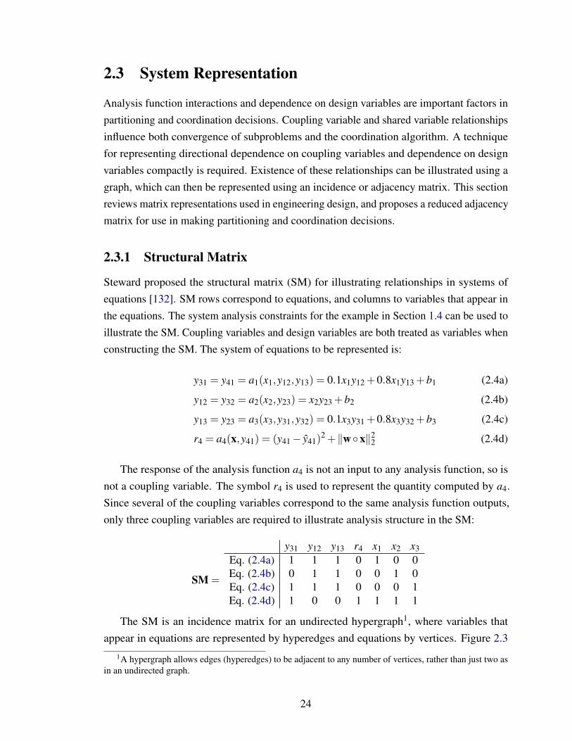
2.3 System Representation
Analysis function interactions and dependence on design variables are important factors inpartitioning and coordination decisions. Coupling variable and shared variable relationshipsinfluence both convergence of subproblems and the coordination algorithm. A techniquefor representing directional dependence on coupling variables and dependence on designvariables compactly is required. Existence of these relationships can be illustrated using agraph, which can then be represented using an incidence or adjacency matrix. This sectionreviews matrix representations used in engineering design, and proposes a reduced adjacencymatrix for use in making partitioning and coordination decisions.
2.3.1 Structural Matrix
Steward proposed the structural matrix (SM) for illustrating relationships in systems ofequations [132]. SM rows correspond to equations, and columns to variables that appear inthe equations. The system analysis constraints for the example in Section 1.4 can be used toillustrate the SM. Coupling variables and design variables are both treated as variables whenconstructing the SM. The system of equations to be represented is:
y31 = y41 = a1(x1,y12,y13) = 0.1x1y12 +0.8x1y13 +b1 (2.4a)
y12 = y32 = a2(x2,y23) = x2y23 +b2 (2.4b)
y13 = y23 = a3(x3,y31,y32) = 0.1x3y31 +0.8x3y32 +b3 (2.4c)
r4 = a4(x,y41) = (y41− y41)2 +‖wx‖22 (2.4d)
The response of the analysis function a4 is not an input to any analysis function, so isnot a coupling variable. The symbol r4 is used to represent the quantity computed by a4.Since several of the coupling variables correspond to the same analysis function outputs,only three coupling variables are required to illustrate analysis structure in the SM:
SM =
y31 y12 y13 r4 x1 x2 x3Eq. (2.4a) 1 1 1 0 1 0 0Eq. (2.4b) 0 1 1 0 0 1 0Eq. (2.4c) 1 1 1 0 0 0 1Eq. (2.4d) 1 0 0 1 1 1 1
The SM is an incidence matrix for an undirected hypergraph1, where variables thatappear in equations are represented by hyperedges and equations by vertices. Figure 2.3
1A hypergraph allows edges (hyperedges) to be adjacent to any number of vertices, rather than just two asin an undirected graph.
24
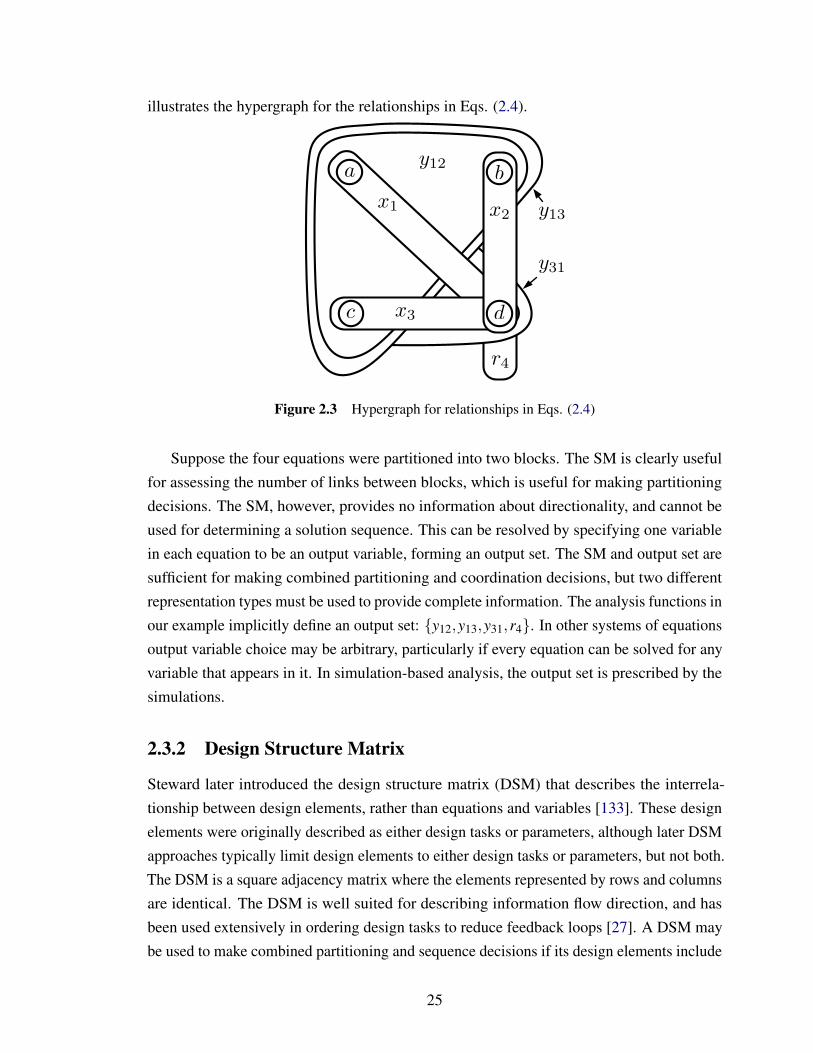
illustrates the hypergraph for the relationships in Eqs. (2.4).
a b
c d
y12
x1 x2
x3
r4
y31
y13
Figure 2.3 Hypergraph for relationships in Eqs. (2.4)
Suppose the four equations were partitioned into two blocks. The SM is clearly usefulfor assessing the number of links between blocks, which is useful for making partitioningdecisions. The SM, however, provides no information about directionality, and cannot beused for determining a solution sequence. This can be resolved by specifying one variablein each equation to be an output variable, forming an output set. The SM and output set aresufficient for making combined partitioning and coordination decisions, but two differentrepresentation types must be used to provide complete information. The analysis functions inour example implicitly define an output set: y12,y13,y31,r4. In other systems of equationsoutput variable choice may be arbitrary, particularly if every equation can be solved for anyvariable that appears in it. In simulation-based analysis, the output set is prescribed by thesimulations.
2.3.2 Design Structure Matrix
Steward later introduced the design structure matrix (DSM) that describes the interrela-tionship between design elements, rather than equations and variables [133]. These designelements were originally described as either design tasks or parameters, although later DSMapproaches typically limit design elements to either design tasks or parameters, but not both.The DSM is a square adjacency matrix where the elements represented by rows and columnsare identical. The DSM is well suited for describing information flow direction, and hasbeen used extensively in ordering design tasks to reduce feedback loops [27]. A DSM maybe used to make combined partitioning and sequence decisions if its design elements include
25
both analysis functions and design variables. The DSM conveniently provides all necessaryinformation in a single representation type. A DSM for the example in Section 1.4 can beconstructed accordingly:
DSM =
a1 a2 a3 a4 x1 x2 x3 x4a1 0 1 1 0 1 0 0 0a2 0 0 1 0 0 1 0 0a3 1 1 0 0 0 0 1 0a4 1 0 0 0 1 1 1 1x1 0 0 0 0 0 0 0 0x2 0 0 0 0 0 0 0 0x3 0 0 0 0 0 0 0 0x4 0 0 0 0 0 0 0 0
The design elements in the above DSM have been grouped into analysis functions anddesign variables, and then ordered by index. This ordering is not necessary; the designelements may appear in an arbitrary order as long as the order of rows and columns areidentical. Strictly speaking, this DSM is the transpose of the adjacency matrix for a directedgraph (digraph) that shows the directional dependence of analysis functions on designvariables and other analysis functions. Existence of an arc between vertices indicates adependence relationship, and the arc direction depicts dependence direction. If a system’sdigraph contains a cycle, then feedback coupling exists. The digraph corresponding to thisDSM is illustrated in Fig. 2.4.
x1 x2
x3
a1 a2
a3 a4
Figure 2.4 Digraph of functional relationships expressed in the DSM
2.3.3 Other Design Matrices
Another related matrix representation is the functional dependence table (FDT), introducedby Wagner [145]. The FDT is similar to the SM, but is intended specifically for partitioning
26

large equation-based design optimization problems. Instead of mapping variables to equa-tions, the FDT maps design and coupling variables to objective and constraint functions.Each row represents a design function, and the columns correspond to design and couplingvariables. The FDT, like the SM, can be viewed as the adjacency matrix for an undirectedhypergraph [105]. It can be used to make partitioning decisions, but lacks directionalityinformation and cannot be used for sequencing decisions without output set specification.The FDT and SM have significant similarities, but the FDT is intended specifically for aidingpartitioning decisions in equation-based engineering design, while the SM applies to generalsystems of equations.
Other matrices associated with engineering design, but normally not used in P/C deci-sions, include the relation matrix (RM) and correlation matrix (CM) from quality functiondeployment [136], and the design matrix (DM) from axiomatic design [135]. The RM mapsproduct engineering characteristics to customer requirements, and the CM describes corre-lations between engineering characteristics. The DM maps design variables to functionalrequirements, and is intended for evaluating independence of functional requirements whencomparing design concepts.
2.3.4 Reduced Adjacency Matrix
A system of analysis functions in simulation-based design may be represented using an SMand an output set, or with a DSM. The latter is convenient because only one representationtype is required. Modifying the DSM can improve its utility in computing metrics forP/C decisions. Taking note that design variables are independent quantities and theircorresponding DSM rows therefore are zero, these rows can be omitted without loss ofinformation. Design elements in the DSM are not constrained to appear in any particularorder. Organizing the matrix such that analysis functions appear before design variablesaids visualization of system structure. In addition, ordering functions and variables byindex value is convenient for calculating metrics used in P/C decisions. This condensed andreordered matrix is termed the reduced adjacency matrix A. The system adjacency matrix is[AT,0]. The reduced adjacency matrix for the example system is:
A =
a1 a2 a3 a4 x1 x2 x3 x4a1 0 1 1 0 1 0 0 0a2 0 0 1 0 0 1 0 0a3 1 1 0 0 0 0 1 0a4 1 0 0 0 1 1 1 1
The reduced adjacency matrix is designed to be consistent with other established notation.
27

In both the reduced adjacency matrix and the DSM, a true element in the i-th row and j-thcolumn indicates the presence of arc 〈 j, i〉. The index order for the elements of A is alsoconsistent with coupling variable index order; i.e., the existence of the coupling variableyi j is signified by a true element in the i-th row and j-th column of the reduced adjacencymatrix. This is consistent with the coupling variable index order set forth by Cramer et al.[35].
The difficulty of solving individual subproblems, as well as the complexity of the co-ordination algorithm, contribute to the overall solution expense, and must be estimatedwhen making P/C decisions. An ideal estimate would account for the nature of analysisfunctions, their interactions, as well as subproblem and coordination algorithms. Produc-ing and analyzing this information in most cases is more computationally intensive thanactually solving the system design problem. More practical estimates are based on moreeasily obtained information. The existence of dependence relationships, expressed in thereduced adjacency matrix, are used to make such estimates. If assumptions are made aboutsubproblem formulations and coordination algorithm, A can be used to estimate the size ofeach subproblem and the coordination problem for a given system partition and coordinationstrategy. Subproblem solution difficulty typically increases with the number of analysisfunctions, design variables, and linking variables, although analysis function properties alsoinfluence difficulty. Similarly, coordination problem solution expense normally increaseswith the number of external consistency constraints [142]. Fine partitions reduce subproblemdifficulty at the expense of more external consistency constraints, while coarse partitionsease coordination difficulty at the cost of more difficult subproblems. Chapters 5 and 7will demonstrated how A can be used to estimate relative contributions of subproblem andcoordination difficulties to overall computational expense.
2.4 Partitioning and Coordination Decision-Making
Partitioning and coordination decisions have been treated largely as two independent tasks.Traditional decision techniques for each are based on guidelines or experience. Formalpartitioning techniques have been studied thoroughly, and draw from strategies in graphpartitioning. Formal coordination decision techniques have been limited to sequence de-cisions. Optimal sequence problems are standard operations research problems. Linkingstructure, the second primary component of coordination decisions, has not yet been studiedthoroughly in the context of decomposition-based design optimization. Analysis of severalformulations for decomposition-based design optimization has led to guidelines for selectingbetween formulations. A few decision methods have linked some aspect of partitioning and
28
coordination interaction, but coupling and tradeoffs present in the combined P/C decisionproblem have not been studied.
2.4.1 Traditional Decision Techniques
Subjective techniques for P/C decisions are in common use. Partitioning techniques willbe discussed first, followed by coordination decision techniques. System design problemscan conveniently be partitioned according to physical system divisions (object-based),or disciplinary divisions within the design organization (aspect-based) [145]. Partitionsmay also follow product, process, or organization divisions [29, 88]. These are typicallysubjective partitioning approaches based on engineering insight.
Design organizations may be aligned by discipline or object, and in some cases by both[36]. Organizational structure can have a profound impact on computational design, sincedesign and analysis tools are developed by parts of the organization, and the organizationrequires tools that are congruent with its actual communication and decision structures.The automotive and aerospace industries have contributed substantially to the developmentof system design methods, and the organizational structure of each industry is reflectedin the methods developed by them. Aerospace design is normally performed by designteams divided by discipline [16], and automotive design organizations usually possess ahierarchical structure aligned by physical subsystems [7]. Discipline-based partitions tendto have a non-hierarchical structure with feedback coupling. Object-based partitions tend tobe hierarchical with unidirectional information flow.
Several authors have cited the importance of choosing the proper formulation for asystem design problem, and some have proposed guidelines for selecting between them[6, 7, 8, 15, 23, 35, 74, 128]. Some of these selection guidelines are based on problemproperties such as coupling strength and problem structure. For example, single-levelmethods, such as IDF, can handle large numbers of shared variables without increasingproblem dimension. Multilevel methods, such as ATC, are a more natural fit for systemswith many local variables, but relatively few shared or coupling variables. Balling andSobieski have explained that single-level methods are best for analysis intensive problems(difficult system or subsystem analysis), while multi-level methods are best for designintensive problems (numerous local decisions to be made) [15]. Wagner identifies severalcategories of problem structure according to FDT representations, and offers suggestionsfor solution method according to which structure type a method matches best [145].
29
2.4.2 Formal Decision Techniques
The traditional techniques outlined above have been useful tools for the sometimes very com-plicated task of determining a system partition and coordination strategy. These techniques,however, are subjective, and success depends on designer experience and insight. Certaininnovative (and possibly superior) solution approaches may be overlooked. The partitioningand sequence decision problems can be solved as optimization problems themselves, andmay be viewed as preprocessing for system optimization. Formal optimization-based tech-niques may reveal insights about the system. Formal partitioning and subproblem sequencemethods have been studied for use in decomposition-based optimization. This sectionreviews important partitioning developments, optimal sequencing techniques, and a fewapproaches that consider some aspect of both partitioning and sequencing.
When a system is represented using a graph, the system partitioning problem can besolved using graph partitioning techniques. Michelena and Papalambros demonstratedthe use of spectral [105] and network reliability methods [103] to obtain partitions thatminimize external linking variables and exactly balance subproblem sizes. Krishnamachariand Papalambros used linear integer programming to generate partitions that allow somesubproblem size imbalance [84]. Chen, Ding, and Li introduced an iterative two-phaseapproach where the FDT is first ordered so that coupling relationships are banded along thediagonal, and then independent variable blocks and a system-wide linking variable blockare formed [30]. Dragan proposed a partitioning algorithm also based on the FDT, as wellas one possible coordination strategy for managing the links between subproblems [47].
Some of the above approaches are decidedly efficient, but require numerous approxima-tions and assumptions. For example, spectral methods can produce a partition in fractionsof second, but require that the FDT hypergraph is approximated with a graph. A linearinteger programming approach is also computationally efficient, but requires significantassumptions to achieve linearity. These methods also do not account for the dimensionof subproblems associated with partition blocks; only the number of analysis function ineach block. Another shortfall is that these methods do not account for directionality infunctional dependence. The consistency constraints for shared and coupling variables arehandled differently in many formulations, and coupling variable consistency constraints areformulated according to functional dependence direction. Omitting directionality from adecision model therefore reduces accuracy.
A large system design problem can take days or weeks to solve. More accurate assump-tions in P/C decision optimization may increase the preprocessing cost to minutes or even afew hours, but the improved P/C decisions stand to decrease system optimization time andincrease reliability of results by a much greater factor; the benefit of added accuracy in P/C
30
decisions may be well worth the cost for decomposition-based design optimization.Sequencing and scheduling problems are standard topics in operations research [22].
Techniques developed for them have been applied to problems in decomposition-baseddesign. A common approach is to order subproblems or design tasks such that feedbackis minimized. Steward used the DSM with a ‘tearing’ algorithm to order design elementsso that blocks of closely coupled tasks can be identified, forming a type of partition. Inthis approach partitions depend on sequence decisions; partitioning decisions cannot bemade independently, and superior P/C decisions may be overlooked. Rogers introducedDeMAID, a heuristic DSM-based software tool for sequencing design tasks [115], andlater DeMAID/GA, which utilized a genetic algorithm [73] to perform sequencing tasks[116]. Browning provided a review of methods based on the DSM [27]. Kroo suggestedthat, after sequencing has been used to minimize feedback loops, consistency constraintscould be used to break any remaining feedback loops [85]. Meier, Yassine, and Browningreviewed DSM-based sequencing approaches and compared their objective functions, whichprimarily involved some combination of minimizing feedback, improving concurrency andmodularity, or reducing computational expense [99]. The above sequencing approaches areprimarily based on the DSM or a similar system representation which models the existenceof functional dependence but does not express the nature of the dependence. A weightedDSM may be used, and Rogers and Bloebaum developed methods for sequencing designtasks that depend on coupling strength metrics, which are based on sensitivities betweendesign tasks [114]. Alyaqout, Papalambros, and Ulsoy defined a new measure of couplingstrength that accounts for optimization algorithm considerations [10]. This metric could alsobe used as a factor in P/C decisions. Most previous approaches for sequencing in designare based only on interactions between analysis functions (i.e., coupling variables). If thesystem representation does not include design variables, and if the decision approach doesnot otherwise account for them, sequence decisions are based on incomplete information.
A few approaches have accounted for some aspect of P/C interaction. Kusiak and Wangdemonstrated a method that first partitions a system based on its FDT, and then identifies anefficient subproblem sequence using a precedence matrix [89]. This is similar to Steward’sSM approach, except that Steward first determined a sequence and then identified a partition.Meier et al. also described how partitions can be identified after a sequence is defined[99]. A sequential P/C decision process, however, cannot account for all P/C decisioninteractions. It will be shown that sequential or independent approaches can fail to identifyPareto-optimal P/C options, while a simultaneous approach does not. Altus, Kroo, and Gagedeveloped a genetic algorithm that simultaneously determined function sequence as wellas ‘breaks’ between functions that form a partition [9]. Only a single result was presented
31
with a prescribed number of subproblems, P/C decision tradeoffs were not studied, andsubproblem order was not defined since parallel subproblem solution was assumed.
Table 2.1 summarizes the partitioning and coordination decision methods reviewedabove. Early formal techniques for partitioning and coordination decisions emphasizedprecedence relationships between analysis functions or design tasks. These precedencerelationships dominated the partitioning problem, and were in effect constraints on partitionsthat could be made. Many approaches based on the DSM, such as Steward’s tearingalgorithm, determine solution sequence first, and then apply heuristic rules or algorithms toderive an associated partition. Most approaches using the DSM are applied to engineeringdesign process scheduling, rather than design optimization, and usually do not accountfor design variables. Later work, including the methods by Michelena and Papalambros,abandoned the use of precedence information in partitioning decisions and focused insteadon function dependence on design variables (represented using the FDT without an outputset). This adds degrees of freedom to the partitioning problem, but disregards informationthat is important both to partitioning and coordination decisions. The work introduced herebrings precedence information back into the decision process. In addition to addressingprecedence relationships among analysis functions, the decision methods presented herealso deal with precedence among subproblems in a coordination strategy. The reducedadjacency matrix was developed as a compact matrix representation that balances precedenceinformation used in early methods with dependence on design variables utilized by morerecent methods. This more complete set of information is used to evaluate the optimizationproblem dimension for each subproblem, something that was only approximated by earliermethods.
The following chapters will describe a technique for optimizing partitioning and coordi-nation decisions based on information contained in the reduced adjacency matrix for theproblem at hand. This technique accounts for the coupling present between partitioningand coordination decisions. Although decisions are based on more complete models thanhave been used in the past, these models are still approximations for computational expense.Therefore the results presented are optimal with respect to the P/C decision model, and areapproximately optimal with respect to computational expense.
Recall that coordination decisions involve both subproblem sequence and consistencyconstraint management; the latter issue has not yet been thoroughly investigated. Differentdistributed design optimization formulations provide varying levels of flexibility in howconsistency constraints may be allocated in a decomposition method (i.e., linking structure).For example, CO completely prescribes allocation, while ATC allows consistency constraintsfor linking variables between subproblems to be assigned to any subproblem that is a
32

Tabl
e2.
1Su
mm
ary
offo
rmal
part
ition
ing
and
coor
dina
tion
deci
sion
met
hods
Met
hod
Rep
rese
ntat
ion
App
licat
ion
Feat
ures
Stew
ard
1965
[132
]te
arin
gSM
,out
puts
etsy
s.of
eqns
.se
quen
ceth
enpa
rtiti
onSt
ewar
d19
81[1
33]
tear
ing
DSM
desi
gnpr
oces
she
uris
tical
gori
thm
Rog
ers
1989
[115
]D
eMA
IDD
SMde
sign
proc
ess
com
mer
cial
lyav
aila
ble
Kus
iak
and
Wan
g19
93[8
9]de
com
posi
tion
FDT,
DSM
desi
gnpr
oces
spa
rtiti
onth
ense
quen
ceR
oger
san
dB
loeb
aum
1994
[114
]su
bpro
b.se
quen
ceD
SMde
sign
opt.
coup
ling
stre
ngth
base
dM
iche
lena
and
Papa
lam
bros
1995
[103
]ne
twor
kFD
Tde
sign
opt.
relia
bilit
ypr
inci
ples
Rog
ers
1996
[116
]D
eMA
ID/G
AD
SMde
sign
proc
ess
gene
tical
gori
thm
Altu
set
al.1
996
[9]
GA
DSM
desi
gnop
t.sc
hedu
ling
and
deco
mp.
Mic
hele
naan
dPa
pala
mbr
os19
97[1
05]
spec
tral
FDT
desi
gnop
t.gr
aph
theo
ryK
rish
nam
acha
rian
dPa
pala
mbr
os19
97[8
4]L
IPFD
Tde
sign
opt.
enab
les
imba
lanc
eD
raga
n20
02[4
7]de
com
posi
tion
FDT
sys.
ofeq
ns.
forp
aral
lelp
roc.
Che
net
al.2
005
two-
phas
eFD
Tde
sign
opt
inde
pend
entb
lock
s
33
common ancestor. ALC offers complete flexibility in consistency constraint allocation,an attractive feature for studying the effect of consistency constraint allocation decisions.Material presented through Chapter 6 only addresses the subproblem sequence aspect ofcoordination decisions, while a more sophisticated approach that considers consistencyconstraints only. Chapter 7 develops the theory required to understand the linking structureaspect of the coordination decision problem and demonstrates how to incorporate linkingstructure into partitioning and coordination decisions.
2.5 Summary
This chapter introduced important concepts from decomposition-based design optimization,which involves partitioning a system design problem into smaller subproblems. System opti-mization methods applied to a decomposed system must ensure that subproblem solutionsare consistent, and that the resulting design is optimal for the overall system. Coordinationstrategies are used to guide repeated subproblem solutions toward a consistent and optimalstate. Subproblem solution sequence and linking structure are aspects of a coordinationstrategy. A system partition and coordination strategy must be defined before solvinga system design optimization problem. Qualitative techniques have been used to guidepartitioning and coordination decisions; formal optimization methods offer an alternativedecision approach, and utilize system structure representations, such as the DSM or FDT.The partitioning problem and the coordination decision problem have been formulatedand solved as independent optimization problems, but have not yet been solved together.Some efforts have involved sequential approaches that account for some, but not all of thecoupling between partitioning and coordination decisions. This dissertation demonstratesthat partitioning and coordination decisions are coupled, and presents an automated decisiontechnique that accounts fully for this coupling. The reduced adjacency matrix introducedin this chapter is a new system representation suitable for making both partitioning andcoordination decisions. The system design problems considered in this dissertation areassumed to be simulation-based with quasiseparable structure. The next chapter introducesseveral system design problems used to demonstrate concepts throughout this dissertation.
34
Chapter 3
Demonstration Examples
Several engineering design optimization problems have been developed to demonstrateconcepts and techniques put forth in this dissertation. All examples are suitable for solvingwith decomposition-based design optimization. Each example has specific properties that areuseful for investigating important aspects of system design, and in most cases partitioningand coordination decisions. A detailed description of the analysis model and design problemfor each example is presented here. Enough detail is provided for most examples to enablereplication. The first example is an air flow sensor design problem with feedback couplingbetween two simple disciplinary analyses. Next, a turbine blade design problem is presentedwith somewhat more sophisticated disciplinary analyses. An approach to designing a productfamily for a fleet of aircraft is then described, which is the only design problem includedhere without sufficient information for problem replication due to reliance on commercialsoftware. The fourth example introduces a generalized approach to truss design which canbe applied to trusses of any size and a large variety of topologies. The last example presentedin this chapter involves the design of an automotive electric water pump. An electric vehicledesign case study is presented later in Chapter 8.
3.1 Air Flow Sensor Design
Vane airflow (VAF) sensors are used in automotive applications to monitor the rate at whichair enters the engine for use in fuel injection control. A VAF sensor design problem wasdeveloped to investigate the effect of coupling between disciplinary analyses. It will beused in Chapter 4 to illustrate two different formulations for decomposition-based designoptimization. The design problem incorporates structural and aerodynamic analyses, andaims at specifying a sensor that produces a desired result to airflow. The operation of a VAFsensor is described, followed by a simplified analysis model for the sensor.
A VAF sensor is illustrated in Fig. 3.1 [34]. Incoming air flows past the stator flap,which deflects in proportion to air flow velocity. A bypass channel reduces the sensor’s
35
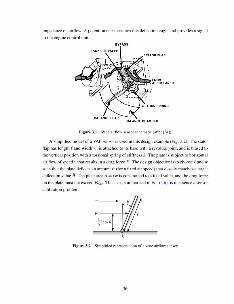
impedance on airflow. A potentiometer measures this deflection angle and provides a signalto the engine control unit.
Figure 3.1 Vane airflow sensor schematic (after [34])
A simplified model of a VAF sensor is used in this design example (Fig. 3.2). The statorflap has length ` and width w, is attached to its base with a revolute joint, and is biased tothe vertical position with a torsional spring of stiffness k. The plate is subject to horizontalair flow of speed v that results in a drag force F . The design objective is to choose ` and w
such that the plate deflects an amount θ (for a fixed air speed) that closely matches a targetdeflection value θ . The plate area A = `w is constrained to a fixed value, and the drag forceon the plate must not exceed Fmax. This task, summarized in Eq. (4.6), is in essence a sensorcalibration problem.
1
2! cos "
v
!F
!
k
Figure 3.2 Simplified representation of a vane airflow sensor
36
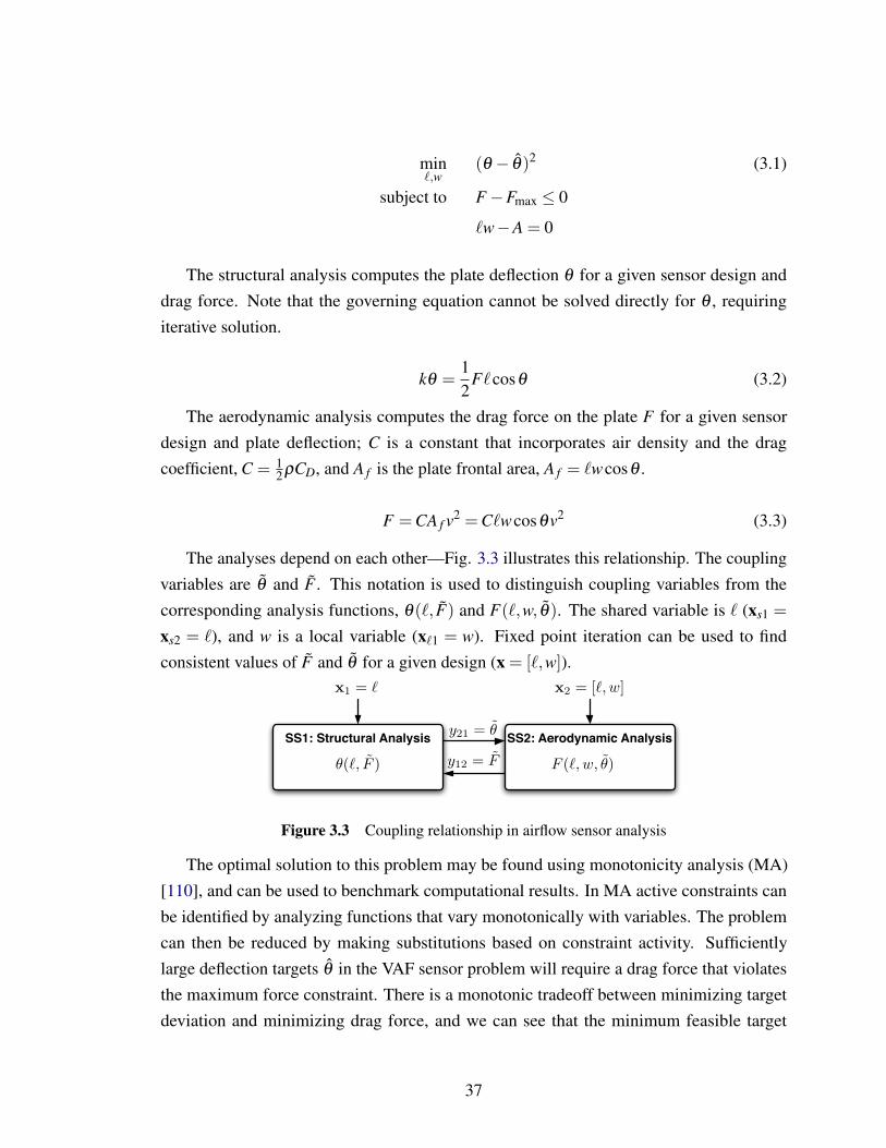
min`,w
(θ − θ)2 (3.1)
subject to F−Fmax ≤ 0
`w−A = 0
The structural analysis computes the plate deflection θ for a given sensor design anddrag force. Note that the governing equation cannot be solved directly for θ , requiringiterative solution.
kθ =12
F`cosθ (3.2)
The aerodynamic analysis computes the drag force on the plate F for a given sensordesign and plate deflection; C is a constant that incorporates air density and the dragcoefficient, C = 1
2ρCD, and A f is the plate frontal area, A f = `wcosθ .
F = CA f v2 = C`wcosθv2 (3.3)
The analyses depend on each other—Fig. 3.3 illustrates this relationship. The couplingvariables are θ and F . This notation is used to distinguish coupling variables from thecorresponding analysis functions, θ(`, F) and F(`,w, θ). The shared variable is ` (xs1 =xs2 = `), and w is a local variable (x`1 = w). Fixed point iteration can be used to findconsistent values of F and θ for a given design (x = [`,w]).
SS1: Structural Analysis SS2: Aerodynamic Analysisy21 = !
y12 = F
x1 = ! x2 = [!, w]
!(", F ) F (!, w, ")
Figure 3.3 Coupling relationship in airflow sensor analysis
The optimal solution to this problem may be found using monotonicity analysis (MA)[110], and can be used to benchmark computational results. In MA active constraints canbe identified by analyzing functions that vary monotonically with variables. The problemcan then be reduced by making substitutions based on constraint activity. Sufficientlylarge deflection targets θ in the VAF sensor problem will require a drag force that violatesthe maximum force constraint. There is a monotonic tradeoff between minimizing targetdeviation and minimizing drag force, and we can see that the minimum feasible target
37

deviation will correspond to the maximum drag force allowed by the inequality constraint.Thus, the drag force constraint is active when the target deflection is large, and we cansubstitute Fmax into Eq. (3.2) to solve for the optimal deflection θ ∗:
θ∗ = cos−1
(Fmax
CA f v2
)(3.4)
The aerodynamics equation and the area constraint can then be used to solve for theoptimal length and width, respectively:
`∗ =2k cos−1
(FmaxCAv2
)CAv2
F2max
, w∗ = A/`∗ (3.5)
For parameter values k = 0.050 N/rad, v = 40.0 m/s, C = 1.00 kg/m3, Fmax = 7.00N, and θ = 0.250 rad, the force constraint is active, and the optimal design is [`∗,w∗] =[0.0365,0.274]. The drag coefficient of a finite flat plate is approximately 2.0, resulting in avalue of C = 1.00 if we assume air density to be 1.00 kg/m3.
The solution of the design problem in Eq. (4.6) requires a nested solution approach. Forevery design proposed by the optimization algorithm, a fixed point iteration solution to Eqs.(3.2) and (3.3) to obtain consistent values for θ and F is required. The solution was obtainedusing a sequential quadratic programming algorithm [69, 111], and the result matches theMA solution.
3.2 Turbine Blade Design
The analysis and design of a turbine blade for a gas turbine engine is presented here.Emphasis is placed on the coupling between structural and thermal analysis, and thisdesign example will be used to study the effects of analysis coupling between disciplinaryanalyses, as was the case with the air flow sensor design problem. This design example wasintroduced in [5] and appeared in [6]. Turbine blade design has been the ongoing subject ofMDO studies [117]. The turbine blade model presented here is simplified enough to allowstraightforward replication, yet still captures important interactions and traddeoffs. Themodel allows for easy adjustment of coupling strength, a feature required for a comparisonof single-level methods presented in Section 4.2.
A turbine blade in a gas turbine engine is exposed to high temperature combustion gassesmoving at high velocity, and is subject to high forces due to aerodynamic drag force andcentripetal acceleration. Figure 3.4 illustrates turbine blades from a GE J-79 turbojet engine[57]. Each blade is attached to the rotor at the left of the figure, and combustion gasses
38
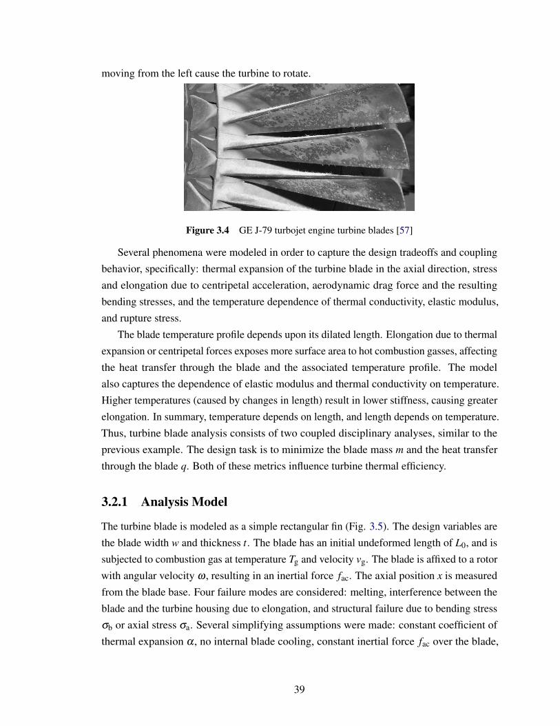
moving from the left cause the turbine to rotate.
Figure 3.4 GE J-79 turbojet engine turbine blades [57]
Several phenomena were modeled in order to capture the design tradeoffs and couplingbehavior, specifically: thermal expansion of the turbine blade in the axial direction, stressand elongation due to centripetal acceleration, aerodynamic drag force and the resultingbending stresses, and the temperature dependence of thermal conductivity, elastic modulus,and rupture stress.
The blade temperature profile depends upon its dilated length. Elongation due to thermalexpansion or centripetal forces exposes more surface area to hot combustion gasses, affectingthe heat transfer through the blade and the associated temperature profile. The modelalso captures the dependence of elastic modulus and thermal conductivity on temperature.Higher temperatures (caused by changes in length) result in lower stiffness, causing greaterelongation. In summary, temperature depends on length, and length depends on temperature.Thus, turbine blade analysis consists of two coupled disciplinary analyses, similar to theprevious example. The design task is to minimize the blade mass m and the heat transferthrough the blade q. Both of these metrics influence turbine thermal efficiency.
3.2.1 Analysis Model
The turbine blade is modeled as a simple rectangular fin (Fig. 3.5). The design variables arethe blade width w and thickness t. The blade has an initial undeformed length of L0, and issubjected to combustion gas at temperature Tg and velocity vg. The blade is affixed to a rotorwith angular velocity ω , resulting in an inertial force fac. The axial position x is measuredfrom the blade base. Four failure modes are considered: melting, interference between theblade and the turbine housing due to elongation, and structural failure due to bending stressσb or axial stress σa. Several simplifying assumptions were made: constant coefficient ofthermal expansion α , no internal blade cooling, constant inertial force fac over the blade,
39
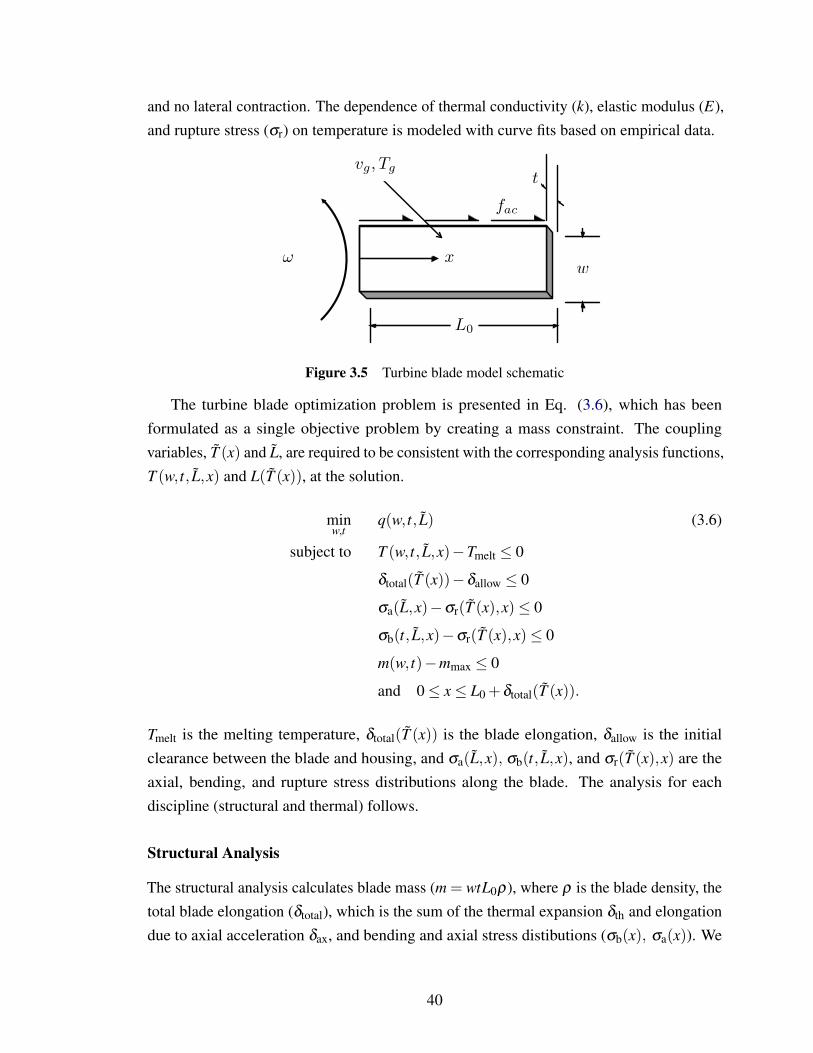
and no lateral contraction. The dependence of thermal conductivity (k), elastic modulus (E),and rupture stress (σr) on temperature is modeled with curve fits based on empirical data.
w
t
L0
x
vg, T
g
facfac
vg, Tg
!
L0
w
x
t
Figure 3.5 Turbine blade model schematic
The turbine blade optimization problem is presented in Eq. (3.6), which has beenformulated as a single objective problem by creating a mass constraint. The couplingvariables, T (x) and L, are required to be consistent with the corresponding analysis functions,T (w, t, L,x) and L(T (x)), at the solution.
minw,t
q(w, t, L) (3.6)
subject to T (w, t, L,x)−Tmelt ≤ 0
δtotal(T (x))−δallow ≤ 0
σa(L,x)−σr(T (x),x)≤ 0
σb(t, L,x)−σr(T (x),x)≤ 0
m(w, t)−mmax ≤ 0
and 0≤ x≤ L0 +δtotal(T (x)).
Tmelt is the melting temperature, δtotal(T (x)) is the blade elongation, δallow is the initialclearance between the blade and housing, and σa(L,x), σb(t, L,x), and σr(T (x),x) are theaxial, bending, and rupture stress distributions along the blade. The analysis for eachdiscipline (structural and thermal) follows.
Structural Analysis
The structural analysis calculates blade mass (m = wtL0ρ), where ρ is the blade density, thetotal blade elongation (δtotal), which is the sum of the thermal expansion δth and elongationdue to axial acceleration δax, and bending and axial stress distibutions (σb(x), σa(x)). We
40
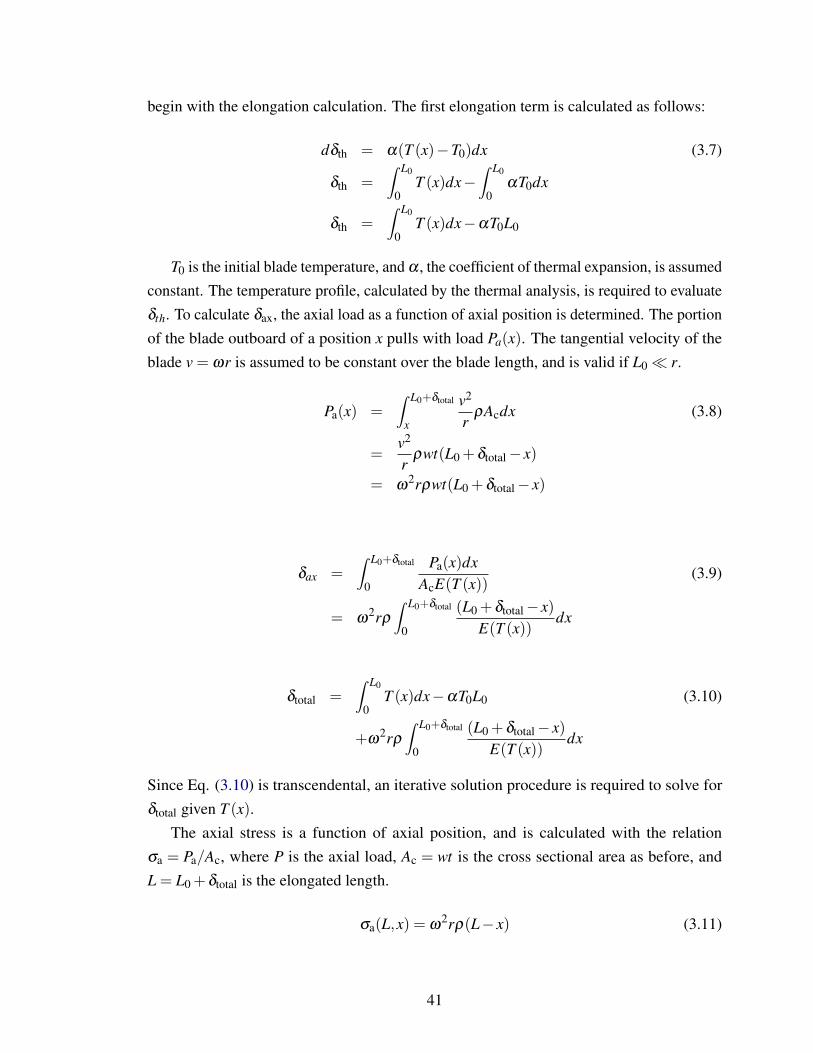
begin with the elongation calculation. The first elongation term is calculated as follows:
dδth = α(T (x)−T0)dx (3.7)
δth =∫ L0
0T (x)dx−
∫ L0
0αT0dx
δth =∫ L0
0T (x)dx−αT0L0
T0 is the initial blade temperature, and α , the coefficient of thermal expansion, is assumedconstant. The temperature profile, calculated by the thermal analysis, is required to evaluateδth. To calculate δax, the axial load as a function of axial position is determined. The portionof the blade outboard of a position x pulls with load Pa(x). The tangential velocity of theblade v = ωr is assumed to be constant over the blade length, and is valid if L0 r.
Pa(x) =∫ L0+δtotal
x
v2
rρAcdx (3.8)
=v2
rρwt(L0 +δtotal− x)
= ω2rρwt(L0 +δtotal− x)
δax =∫ L0+δtotal
0
Pa(x)dxAcE(T (x))
(3.9)
= ω2rρ
∫ L0+δtotal
0
(L0 +δtotal− x)E(T (x))
dx
δtotal =∫ L0
0T (x)dx−αT0L0 (3.10)
+ω2rρ
∫ L0+δtotal
0
(L0 +δtotal− x)E(T (x))
dx
Since Eq. (3.10) is transcendental, an iterative solution procedure is required to solve forδtotal given T (x).
The axial stress is a function of axial position, and is calculated with the relationσa = Pa/Ac, where P is the axial load, Ac = wt is the cross sectional area as before, andL = L0 +δtotal is the elongated length.
σa(L,x) = ω2rρ(L− x) (3.11)
41

The aerodynamic load is calculated using Paero = 12AfCDρv2, where Af = wL is the frontal
area, CD is the drag coefficient, ρ is the combustion gas density, and v is the combustion gasvelocity (assumed perpendicular to the blade). For convenience the constant K = 1
2CDρv2 isdefined, giving Paero = KwL. The total drag force acting on the blade outboard of a positionx is Paero(x) = Kw(L−x), and the bending moment at point x is M(x) = Kw (L−x)2
2 , resultingin a bending stress of:
σb(w,L,x) =3K(L− x)2
4t2 (3.12)
Thermal Analysis
The thermal model, which calculates the temperature profile and heat transfer, was derivedfrom the steady-state heat equation using constant base temperature and an adiabatic tipboundary condition [75]. The average convection coefficient h was approximated usingempirical correlations involving the average Nusselt number Nu and the Prandtl number Pr:Nu = hw
kg= CRez
DPr1/3. The combustion gas conduction coefficient is kg, ReD = vw/ν is theappropriate Reynold’s number, z is an empirical exponent of 0.731, and C is the heat capacityof the combustion gas. Solving for h, and substituting values for the other parameters withSI units (at T∞ = 900C), we find: h(v,w) = 9.196v0.731w−.269. The temperature profile andthe heat transfer through the blade into the rotor at the point of attachment are found throughsolution of the heat equation with the appropriate boundary conditions:
T (w, t,L,x) =cosh(s(L− x))
cosh(sL)(Tb−T∞)+T∞ (3.13)
q(w, t,L) = wt(Tb−T∞) tanh(sL)√
2h(w+ t)wtk (3.14)
where s =√
2h(t +w)/ktw.
Surrogate Models
Surrogate models based on empirical data [97] were employed in order to capture tem-perature dependence. The rupture stress σr for Inconel X-750 was approximated using amodified sigmoid function.
σr(T ) =1300
1+ e0.011(T−675) (3.15)
The conductivity of the blade k was modeled using a linear fit. The dependence on
42
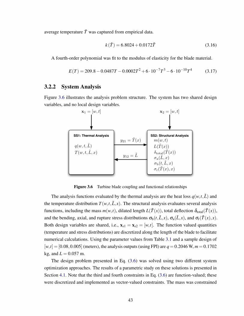
average temperature T was captured from empirical data.
k (T ) = 6.8024+0.0172T (3.16)
A fourth-order polynomial was fit to the modulus of elasticity for the blade material.
E(T ) = 209.8−0.0487T −0.0002T 2 +6 ·10−7T 3−6 ·10−10T 4 (3.17)
3.2.2 System Analysis
Figure 3.6 illustrates the analysis problem structure. The system has two shared designvariables, and no local design variables.
SS1: Thermal Analysis SS2: Structural Analysism(w, t)
x1 = [w, t] x2 = [w, t]
y21 = T (x)
y12 = L
q(w, t, L)
T (w, t, L, x)
L(T (x))!total(T (x))
!b(t, L, x)!a(L, x)
!r(T (x), x)
Figure 3.6 Turbine blade coupling and functional relationships
The analysis functions evaluated by the thermal analysis are the heat loss q(w, t, L) andthe temperature distribution T (w, t, L,x). The structural analysis evaluates several analysisfunctions, including the mass m(w, t), dilated length L(T (x)), total deflection δtotal(T (x)),and the bending, axial, and rupture stress distributions σb(t, L,x), σa(L,x), and σr(T (x),x).Both design variables are shared, i.e., xs1 = xs2 = [w, t]. The function valued quantities(temperature and stress distributions) are discretized along the length of the blade to facilitatenumerical calculations. Using the parameter values from Table 3.1 and a sample design of[w, t] = [0.08,0.005] (meters), the analysis outputs (using FPI) are q = 0.2046 W, m = 0.1702kg, and L = 0.057 m.
The design problem presented in Eq. (3.6) was solved using two different systemoptimization approaches. The results of a parametric study on these solutions is presented inSection 4.1. Note that the third and fourth constraints in Eq. (3.6) are function-valued; thesewere discretized and implemented as vector-valued constraints. The mass was constrained
43
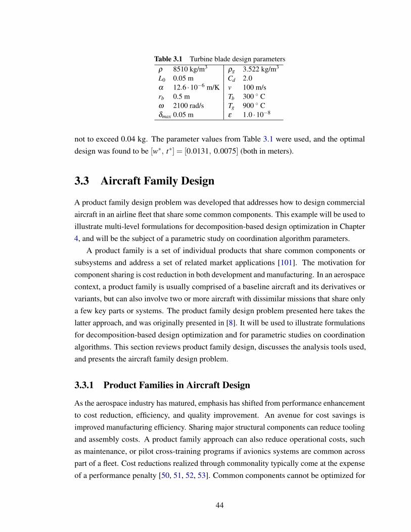
Table 3.1 Turbine blade design parametersρ 8510 kg/m3 ρg 3.522 kg/m3
L0 0.05 m Cd 2.0α 12.6 ·10−6 m/K v 100 m/srb 0.5 m Tb 300 Cω 2100 rad/s Tg 900 Cδmax 0.05 m ε 1.0 ·10−8
not to exceed 0.04 kg. The parameter values from Table 3.1 were used, and the optimaldesign was found to be [w∗, t∗] = [0.0131, 0.0075] (both in meters).
3.3 Aircraft Family Design
A product family design problem was developed that addresses how to design commercialaircraft in an airline fleet that share some common components. This example will be used toillustrate multi-level formulations for decomposition-based design optimization in Chapter4, and will be the subject of a parametric study on coordination algorithm parameters.
A product family is a set of individual products that share common components orsubsystems and address a set of related market applications [101]. The motivation forcomponent sharing is cost reduction in both development and manufacturing. In an aerospacecontext, a product family is usually comprised of a baseline aircraft and its derivatives orvariants, but can also involve two or more aircraft with dissimilar missions that share onlya few key parts or systems. The product family design problem presented here takes thelatter approach, and was originally presented in [8]. It will be used to illustrate formulationsfor decomposition-based design optimization and for parametric studies on coordinationalgorithms. This section reviews product family design, discusses the analysis tools used,and presents the aircraft family design problem.
3.3.1 Product Families in Aircraft Design
As the aerospace industry has matured, emphasis has shifted from performance enhancementto cost reduction, efficiency, and quality improvement. An avenue for cost savings isimproved manufacturing efficiency. Sharing major structural components can reduce toolingand assembly costs. A product family approach can also reduce operational costs, suchas maintenance, or pilot cross-training programs if avionics systems are common acrosspart of a fleet. Cost reductions realized through commonality typically come at the expenseof a performance penalty [50, 51, 52, 53]. Common components cannot be optimized for
44
individual aircraft.The objective of this product family study is to quantify the benefits of a product family
and define the preliminary design of its members. It is critical that the optimization objectivefunction helps quantify the tradeoffs present in product family design problems. Life cyclecost is an ideal objective function, but is unnecessarily complex since an accurate predictionof total cost is not required. An approximate cost model that incorporates both acquisitionand costs was chosen as the objective function. The acquisition cost model, based on[96], is split into manufacturing and development costs. A manufacturing learning curve isapplied such that cost decreases with the number of units produced. Development cost isnon-recurring and is averaged over the total number of aircraft produced. The non-recurringcost for parts already developed for another aircraft in the family is significantly lowerthan for a new part. Fuel cost is based on the Breguet range equation [112]. Each type ofaircraft in the product family is assumed to fly only one specific mission. The acquisitionand fuel cost models are used to estimate ticket prices for each aircraft in the context of fleetoperation. Important tradeoffs associated with commonality are effectively captured by theticket price estimates.
3.3.2 Aircraft Performance Analysis
Aircraft performance is evaluated using the Program for Aircraft Synthesis Studies (PASS),an aircraft conceptual design tool [87]. A detailed description of this analysis is beyond thescope of this dissertation, and is presented in [86]. In addition to quantities computed byPASS, the aircraft family problem requires calculation of wing stresses. The wing modeluses wing geometry design variables, such as wing sweep (Λ) and main wing aspect ratio(ARmw), as well as aircraft takeoff weight WTO, as inputs to a simple wing-box model wherewing skin carried the bending load. If wing skin thickness along the wing span is designedsuch that the wing is fully stressed, the skin thickness is approximately quadratic along thespan. This observation allows us to parameterize skin thickness along the entire main wingspan using only three thickness values: T1 (thickness at wing root), T2 (thickness at 33%span), and T3 (thickness at 67% span). The main wing is the only common component inthis product family study: wing tip extensions can be unique for each aircraft. Wing weightis also influenced by the minimum gauge of available material and control surfaces andhigh-lift systems. Equation (3.18) accounts for these factors as well as minimum bendingthickness was fit to data from existing aircraft.
Wwing = 1.35(Wstr−Wmin)+4.9Swing. (3.18)
45
where Wstr is the weight of material needed to resist bending, Wmin is the weight of minimumgauge material, and Swing is the wing area.
3.3.3 Aircraft Family Problem Formulation
The product family considered here is limited to two aircraft types, A and B, designed tofulfill missions 1 and 2, respectively. Mission 1 requires a range of 3400 nautical miles (nmi)and an aircraft capacity of 296 passengers. Mission 2 requires a range of 8200 nmi and anaircraft capacity of 259 passengers. Forecasts suggest a market need for 800 type A aircraft,and a need for 400 type B aircraft. In addition to mission requirements, constraints on otherperformance metrics, such as balanced field length and second segment climb, are included.
The aircraft family design problem is to minimize a composite cost measure for the fleet,subject to mission and performance constraints, as well as compatibility of common parts.Each aircraft type has 16 design variables (x1i . . .x16i, i ∈ A,B), which are described inTable 3.2.
Main wing commonality requires that the variables x10i . . .x16i are equal for each aircraft.This requirement can be met by treating them as shared variables:
xs = [x10A, . . . ,x16A] = [x10B, . . . ,x16B]. (3.19)
The local variables for aircraft A and B are
x`A = [x1A, . . . ,x9A] and x`B = [x1B, . . . ,x9B].
The complete set of design variables for the product family design problem is
x = [x`A, x`B, xs].
Each aircraft must comply with a set of five performance constraints, whose numericvalues are specific to the mission each aircraft is designed to fly (see Table 3.3).
The fleet composite cost metric is given in Eq. (3.20), and is the aircraft family designobjective function. It is based on estimated ticket prices and the proportion of aircraft typesin the fleet. The estimated ticket prices for aircrafts A and B are pA and pB, respectively, andthe number of aircraft A and B in the fleet are nA and nB, respectively.
f (x) =nA
nA +nBpA(x`A,xs)+
nB
nA +nBpB(x`B,xs). (3.20)
The elements of the aircraft family design problem have all been defined now. The
46
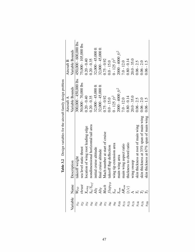
Tabl
e3.
2D
esig
nva
riab
les
fort
heai
rcra
ftfa
mily
desi
gnpr
oble
mA
ircr
aftA
Air
craf
tBV
aria
ble
Nam
eD
escr
iptio
nV
aria
ble
Bou
nds
Var
iabl
eB
ound
sx 1
iW
TO
take
offw
eigh
t30
0,00
0-4
50,0
00lb
s45
0,00
0-6
00,0
00lb
sx 2
ith
rust
sea
leve
lsta
ticth
rust
50,0
00-7
0,00
0lb
s75
,000
-105
,000
lbs
x 3i
X win
glo
catio
nof
win
gro
otle
adin
ged
ge0.
20-0
.40
0.20
-0.4
0x 4
iS h
/Sre
fno
ndim
ensi
onal
hori
zont
alta
ilar
ea0.
20-0
.35
0.20
-0.3
5x 5
iA
lt Iin
itial
crui
seal
titud
e32
,000
-45,
000
ft32
,000
-45,
000
ftx 6
iA
lt Ffin
alcr
uise
altit
ude
32,0
00-4
5,00
0ft
32,0
00-4
5,00
0ft
x 7i
Mac
hM
ach
num
bera
tsta
rtof
crui
se0.
75-0
.92
0.75
-0.9
2x 8
ifl
apT
Ota
keof
fflap
defle
ctio
n0.
0-1
5.0
0.0
-15.
0x 9
iS w
tw
ing
tipex
tens
ion
area
0-1
25ft
20
-125
ft2
x 10i
S wm
mai
nw
ing
area
2000
-400
0ft
220
00-4
000
ft2
x 11i
AR
wm
mai
nw
ing
aspe
ctra
tio7.
0-1
2.0
7.0
-12.
0x 1
2i(t
/c)
thic
knes
sto
chor
dra
tio0.
80-0
.14
0.80
-0.1
4x 1
3iΛ
win
gsw
eep
20.0
-35.
020
.0-3
5.0
x 14i
T 1sk
inth
ickn
ess
atro
otof
mai
nw
ing
0.06
-2.5
0.06
-2.5
x 15i
T 2sk
inth
ickn
ess
at33
%sp
anof
mai
nw
ing
0.06
-2.0
0.06
-2.0
x 16i
T 3sk
inth
ickn
ess
at67
%sp
anof
mai
nw
ing
0.06
-1.5
0.06
-1.5
47
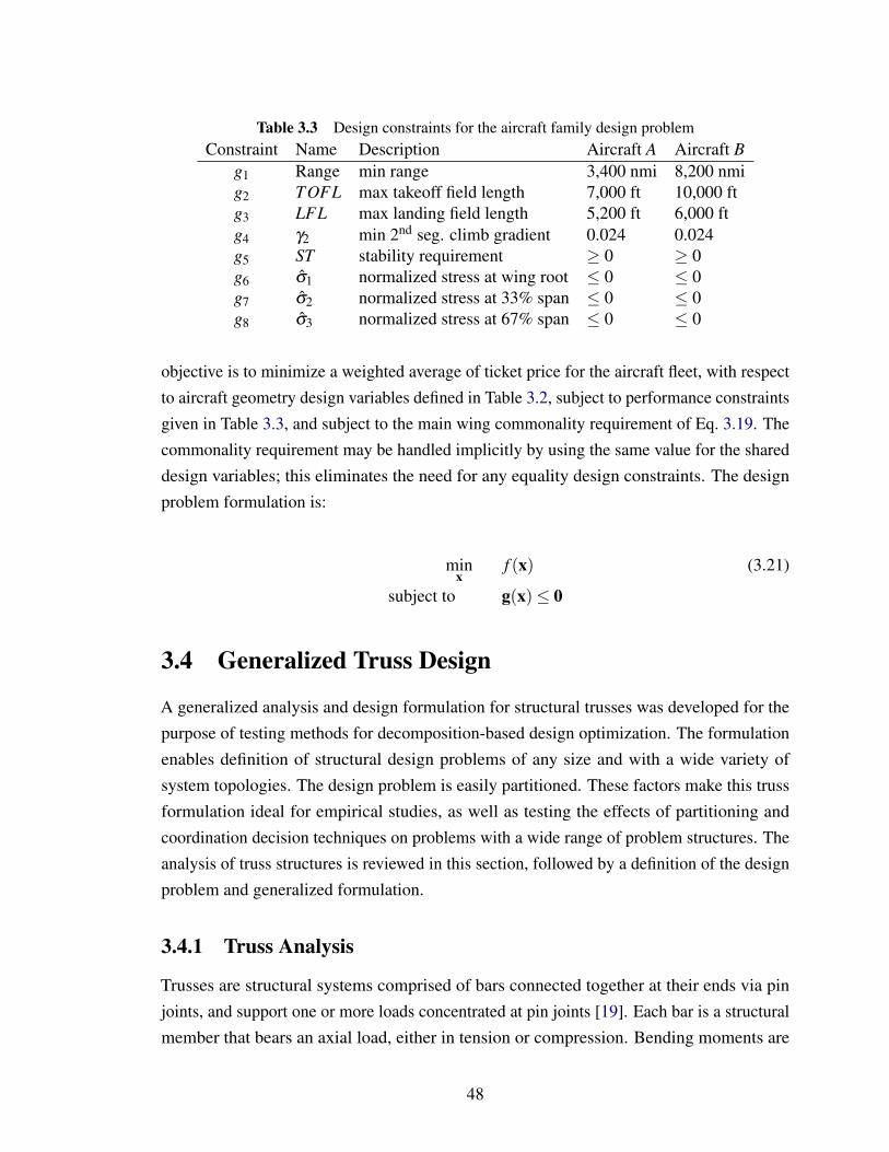
Table 3.3 Design constraints for the aircraft family design problemConstraint Name Description Aircraft A Aircraft B
g1 Range min range 3,400 nmi 8,200 nmig2 TOFL max takeoff field length 7,000 ft 10,000 ftg3 LFL max landing field length 5,200 ft 6,000 ftg4 γ2 min 2nd seg. climb gradient 0.024 0.024g5 ST stability requirement ≥ 0 ≥ 0g6 σ1 normalized stress at wing root ≤ 0 ≤ 0g7 σ2 normalized stress at 33% span ≤ 0 ≤ 0g8 σ3 normalized stress at 67% span ≤ 0 ≤ 0
objective is to minimize a weighted average of ticket price for the aircraft fleet, with respectto aircraft geometry design variables defined in Table 3.2, subject to performance constraintsgiven in Table 3.3, and subject to the main wing commonality requirement of Eq. 3.19. Thecommonality requirement may be handled implicitly by using the same value for the shareddesign variables; this eliminates the need for any equality design constraints. The designproblem formulation is:
minx
f (x) (3.21)
subject to g(x)≤ 0
3.4 Generalized Truss Design
A generalized analysis and design formulation for structural trusses was developed for thepurpose of testing methods for decomposition-based design optimization. The formulationenables definition of structural design problems of any size and with a wide variety ofsystem topologies. The design problem is easily partitioned. These factors make this trussformulation ideal for empirical studies, as well as testing the effects of partitioning andcoordination decision techniques on problems with a wide range of problem structures. Theanalysis of truss structures is reviewed in this section, followed by a definition of the designproblem and generalized formulation.
3.4.1 Truss Analysis
Trusses are structural systems comprised of bars connected together at their ends via pinjoints, and support one or more loads concentrated at pin joints [19]. Each bar is a structuralmember that bears an axial load, either in tension or compression. Bending moments are
48
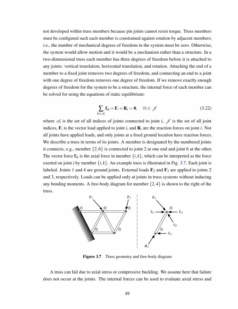
not developed within truss members because pin joints cannot resist torque. Truss membersmust be configured such each member is constrained against rotation by adjacent members;i.e., the number of mechanical degrees of freedom in the system must be zero. Otherwise,the system would allow motion and it would be a mechanism rather than a structure. In atwo-dimensional truss each member has three degrees of freedom before it is attached toany joints: vertical translation, horizontal translation, and rotation. Attaching the end of amember to a fixed joint removes two degrees of freedom, and connecting an end to a jointwith one degree of freedom removes one degree of freedom. If we remove exactly enoughdegrees of freedom for the system to be a structure, the internal force of each member canbe solved for using the equations of static equilibrium:
∑k∈Ai
fik +Fi +Ri = 0, ∀i ∈J (3.22)
where Ai is the set of all indices of joints connected to joint i, J is the set of all jointindices, Fi is the vector load applied to joint i, and Ri are the reaction forces on joint i. Notall joints have applied loads, and only joints at a fixed ground location have reaction forces.We describe a truss in terms of its joints. A member is designated by the numbered jointsit connects, e.g., member 2,6 is connected to joint 2 at one end and joint 6 at the other.The vector force fik is the axial force in member i,k, which can be interpreted as the forceexerted on joint i by member i,k. An example truss is illustrated in Fig. 3.7. Each joint islabeled. Joints 1 and 4 are ground joints. External loads F2 and F3 are applied to joints 2and 3, respectively. Loads can be applied only at joints in truss systems without inducingany bending moments. A free-body diagram for member 2,4 is shown to the right of thetruss.
1 2 3
4 5
F3F2
4
2
F2
f23
f25
f45
f21
R4
Figure 3.7 Truss geometry and free-body diagram
A truss can fail due to axial stress or compressive buckling. We assume here that failuredoes not occur at the joints. The internal forces can be used to evaluate axial stress and
49
failure conditions. The truss members are assumed to have a circular cross sections, andto be made of an isotropic material with stiffness modulus E. The axial stress of memberi, j is
σi j =‖fi j‖2
πr2i j
(3.23)
where ri j is the section radius of member i, j. The axial stress must not exceed the materialfailure stress σallow. Axial stress is normally the failure mode only when the member is intension. Long, slender truss members tend to exhibit buckling failure before the axial stressreaches σallow. High axial compression can cause an unstable condition where perturbing amember in the lateral direction will cause a lateral deflections to increase without bound[59]. The equation governing the lateral deflection v of member i, j with pin joints at eachend under a compressive axial load P is
EIv′′+Pv = 0 (3.24)
where I is the area moment of inertia for the member section. For a circular section,I = πr2
i j/4. According to Euler buckling theory, buckling can occur when the solution toEq. (3.24) v is non-zero. This requires that sin(nπL) = 0, where L is the member length andn = 1,2,3, . . .. The first mode of the solution to Eq. (3.24) occurs when n = 1, and thecorresponding axial load is:
Pcr =π2EI
L2 (3.25)
Pcr is the smallest compressive axial load under which buckling will occur accordingto Euler buckling theory. The largest compressive axial load that member i, j can bearbefore the possibility of buckling in our model is:
bi j =π3r4
i jE
4L2 (3.26)
Some truss structures are over-constrained; they have more kinematic constraints thannecessary to ensure zero degrees of freedom. The number of unknown forces exceeds thenumber of equilibrium equations. The internal forces cannot be solved from static equilib-rium conditions alone, and therefore these structures are termed statically indeterminate.This problem can be resolved by including additional compatibility equations that relateinternal forces to deformed joint positions. The larger system of equations that results canbe solved for the internal forces and deformed joint positions. The undeformed (original)location of joint i is the vector ui = [uxi,uyi], and the deformed location of joint i after
50
load application is di = [dxi,dyi]. It is helpful to relate the vector form of the axial force inmember i, j to the magnitude of this force fi j = ‖fi j‖2 and the deformed location of itsjoints, as shown in Eq. (3.27).
fi j = fi jd j−di
‖d j−di‖2(3.27)
Note that the force exerted by member i, j on joint j is f ji =−fi j. The compatibilityequations ensure that the member ends connected to the same joint are collocated afterdeformation:
‖di−d j‖2−‖ui−u j‖2−fi j‖ui−u j‖2
πr2i jE
= 0, ∀i, j ∈M (3.28)
where M is the set of all unordered member index pairs. Note that the ordered pair J ,M comprises an undirected graph that describes truss topology.
3.4.2 Truss Design Formulation
The class of trusses considered in this generalized formulation include those with memberssecured via joints at each end, with two or more fixed ground joints, and at least one load isapplied to a non-ground joint. Topologies that exhibit static indeterminacy are allowed in thisformulation. In the design problem, not only can member radii be varied, but the position ofcertain joints can be specified. Thus, the design problem is a sizing and shape optimizationproblem. Joints whose undeformed locations are design variables, i.e., movable joints, arethose that are not ground joints and have no applied loads. For convenience, the indices ofall fixed ground joints is defined as the set G , and the set of all joint indices with an appliedexternal load force is L . The vector of all movable joint locations is m = [ui1,ui1, . . . ,uik ],where i1, i2, . . . , ik= J \(G ∪L ), and k = |J \(G ∪L )|.
The truss design problem is to select the radii of all members r and positions of allmovable joints m such that the system mass is minimized without violating axial stressor buckling constraints. Ground and load joints have prescribed locations in the designproblem, but the other joints are considered moveable. Since statically indeterminate systemsare allowed, both structural compatibility and joint equilibrium equations are includedin the analysis. State variables include internal member forces (f = [ fi1 j1, fi2 j2, . . . , fik jk ],i1, j1,i2, j2, . . . ,ik, jk= M , and k is the number of truss members), the deformedpositions of non-ground joints (d = [di1,di2 , . . . ,dik ] where i1, i2, . . . , ik = J \G andk = |J \G |), and the reaction forces (R = [Ri1,Ri2, . . . ,Ri|G |], i1, i2, . . . , i|G | = G ). Theall-at-once (AAO) optimization formulation [35] for the general truss design problem
51
includes both design (m,r) and state (f, d,R) variables as decision variables, and treats stateequations as equality constraints:
minm,r,f,d,R
∑i, j∈M
Ωi j (3.29)
subject to: |σi j|−σallow ≤ 0, ∀i, j ∈M
− fi j−bi j ≤ 0, ∀i, j ∈M
‖di−d j‖2−‖ui−u j‖2−fi j‖ui−u j‖2
πr2i jE
= 0, ∀i, j ∈M
∑k∈Ai
fik +Fi +Ri = 0, ∀i ∈J
where: σi j =fi j
πr2i j
, bi j =π3r4
i jE
4‖ui−u j‖22, Ωi j = ρπr2
i j‖ui−u j‖2
Design parameters include material density ρ , elastic modulus E, allowable stress σallow,fixed ground and load joint positions (di,∀i ∈ G ∪L ), and applied loads (Fi,∀i ∈L ). Themass of member i, j is Ωi j. A specific truss design example with eight members and twoloads is presented in Section 6.3, and is used to demonstrate an evolutionary algorithm [49]for making partitioning and coordination decisions.
3.5 Electric Water Pump Design
This section describes a design optimization model for an automotive water (coolant) pumpdriven by a DC electric motor. It involves several strongly interacting analysis functions,and is suitable for use as a test problem for decomposition-based design optimization. Itis used in Chapter 5 to demonstrate a deterministic approach to optimal partitioning andcoordination decision-making, and is again used in Chapter 6 to compare the results of anevolutionary algorithm against deterministic results.
The analysis functions in the model for the electric water pump design problem arebased on sets of explicit algebraic equations. A similar model was presented in [7] thatinvolved the design of a belt-driven electric sump pump. The model presented here is moresophisticated, and uses an alternative approach to solve for the steady state operating speed.In [7] the analysis functions generated torque-speed curves for the pump and motor, andthen solved for the intersection of those curves to find the operating point. Generatingthese curves was costly, but eliminated some of the feedback coupling between analysisfunctions. In this model the operating speed is treated as a coupling variable, and insteadof determining the operating speed via torque-speed curves, it is solved for as an unknown
52

state variable. This results in strong coupling between analysis functions, but makes for amore interesting analysis structure that can be used for the analysis of decomposition-baseddesign optimization methods as well as in the study of partitioning and coordination decisionapproaches.
3.5.1 Water Pump Design
Traditional automotive water pumps are belt driven by the vehicle engine, constrainingpump shaft speed to engine speed multiplied by the belt speed ratio. In some cases, suchas when a vehicle is idling after a period of high load, the water pump must provide flowand pressure sufficient to cool a hot engine at low shaft speeds. Pumps can be designed tooperate efficiently at a specific operating point, but cannot be simultaneously efficient athigh and low shaft speeds. An engine-driven pump operates at off-design flow conditionsduring much of its duty cycle due to large speed fluctuations. This characteristic of belt-driven pumps results in higher power consumption than pumps driven by a constant-speedsource. A motor-driven pump can provide constant input speed, and further reduces energyconsumption by only pumping when needed. Traditional water pumps are run continuouslyand utilize a thermostat-controlled bypass when engine cooling is not required.
Electrification of belt-driven automotive components is a promising means for improvingfuel economy. Electrification of some components, such as cooling fans, has been incorpo-rated for some time into production vehicles. Electrification of additional components is amore recent endeavor [77, 82, 98]. Surampudi et al. tested a speed-controlled electric waterpump on a class-8 tractor and measured an 80% reduction in energy consumption [137].
The analysis model used in this design problem involves five interdependent analysisfunctions that compute performance metrics based on ten design variable values. Thesequantities are defined in Table 3.4. Design variables x1–x5 define motor geometry, andx6–x10 define pump geometry. The motor is a permanent magnet brushed DC electric motorwith four pole pairs, and the pump is single-stage centrifugal with six impeller blades and asingle diffuser vane (Fig. 3.8). The motor directly drives the pump, so their shaft speeds areidentical: ωmotor = ωpump = ω .
Several analysis interactions are modeled. For example, the temperature is computedbased on the motor current and speed, but the temperature affects the electrical resistanceand current, and the current influences the motor speed. The interdependence betweenanalysis functions is illustrated in Fig. 3.9. Since pump pressure P and input shaft torque τ
depend on identical sets of design variables and analysis outputs, only τ is included in thegraph for simplicity and represents both P and τ calculations.
53
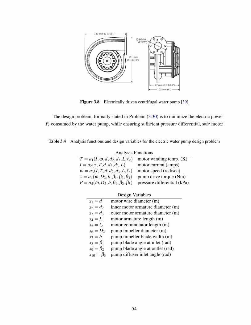
Figure 3.8 Electrically driven centrifugal water pump [39]
The design problem, formally stated in Problem (3.30) is to minimize the electric powerPe consumed by the water pump, while ensuring sufficient pressure differential, safe motor
Table 3.4 Analysis functions and design variables for the electric water pump design problem
Analysis FunctionsT = a1(I,ω,d,d2,d3,L, `c) motor winding temp. (K)I = a2(τ,T,d,d2,d3,L) motor current (amps)ω = a3(I,T,d,d2,d3,L, `c) motor speed (rad/sec)τ = a4(ω,D2,b,β1,β2,β3) pump drive torque (Nm)P = a5(ω,D2,b,β1,β2,β3) pressure differential (kPa)
Design Variablesx1 = d motor wire diameter (m)x2 = d2 inner motor armature diameter (m)x3 = d3 outer motor armature diameter (m)x4 = L motor armature length (m)x5 = `c motor commutator length (m)x6 = D2 pump impeller diameter (m)x7 = b pump impeller blade width (m)x8 = β1 pump blade angle at inlet (rad)x9 = β2 pump blade angle at outlet (rad)x10 = β3 pump diffuser inlet angle (rad)
54
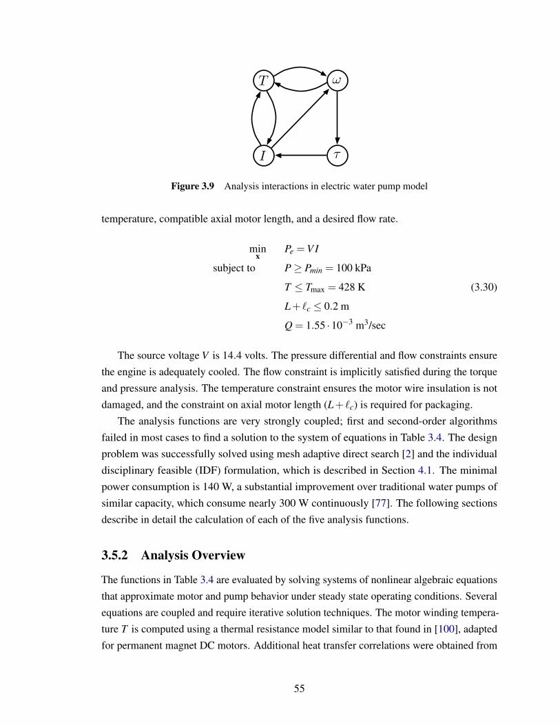
T !
I !
Figure 3.9 Analysis interactions in electric water pump model
temperature, compatible axial motor length, and a desired flow rate.
minx
Pe = V I
subject to P≥ Pmin = 100 kPa
T ≤ Tmax = 428 K (3.30)
L+ `c ≤ 0.2 m
Q = 1.55 ·10−3 m3/sec
The source voltage V is 14.4 volts. The pressure differential and flow constraints ensurethe engine is adequately cooled. The flow constraint is implicitly satisfied during the torqueand pressure analysis. The temperature constraint ensures the motor wire insulation is notdamaged, and the constraint on axial motor length (L+ `c) is required for packaging.
The analysis functions are very strongly coupled; first and second-order algorithmsfailed in most cases to find a solution to the system of equations in Table 3.4. The designproblem was successfully solved using mesh adaptive direct search [2] and the individualdisciplinary feasible (IDF) formulation, which is described in Section 4.1. The minimalpower consumption is 140 W, a substantial improvement over traditional water pumps ofsimilar capacity, which consume nearly 300 W continuously [77]. The following sectionsdescribe in detail the calculation of each of the five analysis functions.
3.5.2 Analysis Overview
The functions in Table 3.4 are evaluated by solving systems of nonlinear algebraic equationsthat approximate motor and pump behavior under steady state operating conditions. Severalequations are coupled and require iterative solution techniques. The motor winding tempera-ture T is computed using a thermal resistance model similar to that found in [100], adaptedfor permanent magnet DC motors. Additional heat transfer correlations were obtained from
55

[75]. The motor current I and shaft speed ω are computed based on fundamental DC motorequations [78, 60] adapted to the specific geometry of this motor. The pump drive torqueand pressure differential are computed for a prescribed flow rate Q using fluid mechanicsequations for centrifugal pumps [144]. Model parameters used in this analysis are listedin Table 3.5. Motor and pump geometry will be described, followed by description of theanalysis equations. Full description of the physics underlying the equations presented canbe found in the references.
Table 3.5 Electric water pump model parameters
δa 0.002 motor air gap (m)δh 0.010 motor housing thickness (m)d1 0.008 motor shaft diameter (m)g 9.81 gravitational constant (m/s2)T∞ 350 engine compartment temp. (K)na 1.50 slot/tooth ratiop 4 one-half number of polesnp 0.55133 wire packing ratioµ0 18.27e-6 viscosity constant (Pa·s)T0 291.15 base temperature (K)C 120 viscosity parameter (K)Cp 1.009 air heat capacity (kJ/kg·K)Br 0.10 remanent magnetic flux density (T)V 14.4 source voltage (V)Ds 0 pump shaft diameter (m)D1 0.020 impeller inlet diameter (m)D3 0.150 volute throat mean inlet diameter (m)D4 0.032 exit flange inner diameter (m)nB 6 no. impeller bladesnV 1 no. diffuser vanesb3 0.032 diffuser inlet width (m)ρc 970 coolant density (kg/m3)Q 0.00155 flow rate (m3/s)CDF 1 ·10−7 disk friction coefficient (m2s2/kg)CSF 5 ·10−3 skin friction coefficient (m−1)CVD 0.5 diffuser loss coefficientCin 0.8 diffuser approach coefficient
Motor Geometry
Figure 3.10 provides a side section view of the DC motor. The iron-cored armature, or rotor,of the DC motor rotates within cylindrical permanent magnets with remanent magnetic fluxdensity Br. The outer armature diameter is d3, the armature axial length is L, and the gap
56

between the armature and magnets is δa. The thickness of the magnets is δh. A shaft ofdiameter d1 runs through the armature and is supported by bearings at each end of the motorhousing. The commutator is a mechanical switch that routes electrical current through thecorrect armature windings at the appropriate time as the motor rotates. Stationary brushessliding on the commutator provide the means for electrical conduction (brushes not shown).The commutator is mounted on the motor shaft and has outer diameter dc and axial length`c.
Armature geometry is approximated as shown in Fig. 3.11. Insulated copper windingswith diameter d run through each of the 2p = 8 armature slots, where p is the number ofmagnetic pole pairs. Each slot has a depth of (d3−d2)/2 and subtends the angle θs. Thearmature teeth separate the windings and each tooth subtends an angle of θt .
d1 !a !h
!c
dc d3
L
Lh
armaturefield magnet
commutator
Figure 3.10 Schematic of permanent magnet DC motor
Pump Geometry
Figure 3.12 illustrates the geometry of the centrifugal water pump. The drive shaft ofdiameter Ds rotates the impeller, which has nB = 6 blades. Coolant flows in through the inletof diameter D1 and is expelled radially outwards due to impeller rotation. As the coolantflows through the diffuser its velocity is reduced, but it experiences an increase in pressureaccording to Bernoulli’s principle. The outer impeller diameter is D2, and the volute inletdiameter is D3. The inlet impeller blade angle is β1, and the outlet impeller blade angle isβ2. The diffuser inlet blade angle (not shown) is β3. The exit flange diameter is D4. Theimpeller blade width is b and the diffuser inlet width is b3.
57
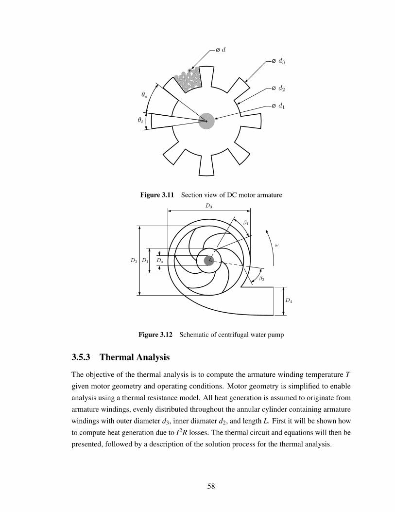
Ø
Ø
Ø
Ø
!s
!t
d
d1
d2
d3
Figure 3.11 Section view of DC motor armature
Ds
D3
D1D2
D4
!1
!2
!
Figure 3.12 Schematic of centrifugal water pump
3.5.3 Thermal Analysis
The objective of the thermal analysis is to compute the armature winding temperature T
given motor geometry and operating conditions. Motor geometry is simplified to enableanalysis using a thermal resistance model. All heat generation is assumed to originate fromarmature windings, evenly distributed throughout the annular cylinder containing armaturewindings with outer diameter d3, inner diamater d2, and length L. First it will be shown howto compute heat generation due to I2R losses. The thermal circuit and equations will then bepresented, followed by a description of the solution process for the thermal analysis.
58
Wire Length and Heat Generation
Calculation of heat generation requires knowledge of armature electrical resistance, whichdepends on total wire length and wire temperature. The model for wire length assumes wind-ings are made around each armature tooth, and accounts for wire curvature and extensionbeyond armature ends. The slot to tooth volume ratio, na = θs/θt , is assumed to be fixed at1.5. The total volume occupied by wire passing through the slots Vs can be calculated usingthe following formulae:
θs = π/p(1+1/na), θt = θs/na, θp = θs +θt
As = θs(d23−d2
2)/8, Vs = npAsL
where θp is the angle between poles, As is the section area of each slot, and np = 0.55133 isthe packing ratio, i.e., the ratio of wire volume occupying slots to total slot volume. Theratio np was calculated based on close packing geometry. Aw = πd2/4 is the sectional areaof a single wire, and the total length of wire passing through armature slots is `s = Vs/Aw.The total number of winding turns for all poles is nt = `s/2L. In reality nt is integer valued,but is assumed to be relaxed to a continuous number here. This provides a reasonableapproximation when nt is large. The average wire length between slots for each windingturn is ¯e = θs(1/na +π/4)(d2+d3)/4, and the total length of wire is:
` = `s +2 ¯ent (3.31)
The resistivity of copper varies with temperature, and is approximated using a linearmodel:
ρ(T ) = 1.72 ·10−8(1+0.00393(T −293)) (3.32)
The total heat generated by the armature windings due to I2R losses is:
S = 4ρ`I2/πd2 (3.33)
Thermal Resistance Model
The thermal resistance model used in this analysis to calculate wire temperature T isillustrated in Fig. 3.13. The heat source is the annulus ring of the armature containing thewindings, and the thermal sink is the engine compartment at temperature T∞.
The first path in the circuit passes through R1, R2, and R3, and represents the thermalpath directly from the armature through the air gap, magnets, and housing to the engine
59
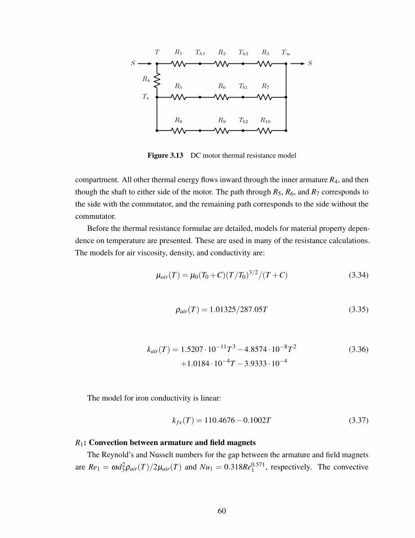
S
T R1 R2 R3
R4
R5 R6 R7
R8 R9 R10
T!Th1 Th2
Ts
Tb1
Tb2
S
Figure 3.13 DC motor thermal resistance model
compartment. All other thermal energy flows inward through the inner armature R4, and thenthough the shaft to either side of the motor. The path through R5, R6, and R7 corresponds tothe side with the commutator, and the remaining path corresponds to the side without thecommutator.
Before the thermal resistance formulae are detailed, models for material property depen-dence on temperature are presented. These are used in many of the resistance calculations.The models for air viscosity, density, and conductivity are:
µair(T ) = µ0(T0 +C)(T/T0)3/2/(T +C) (3.34)
ρair(T ) = 1.01325/287.05T (3.35)
kair(T ) = 1.5207 ·10−11T 3−4.8574 ·10−8T 2 (3.36)
+1.0184 ·10−4T −3.9333 ·10−4
The model for iron conductivity is linear:
k f e(T ) = 110.4676−0.1002T (3.37)
R1: Convection between armature and field magnetsThe Reynold’s and Nusselt numbers for the gap between the armature and field magnets
are Re1 = ωd23ρair(T )/2µair(T ) and Nu1 = 0.318Re0.571
1 , respectively. The convective
60
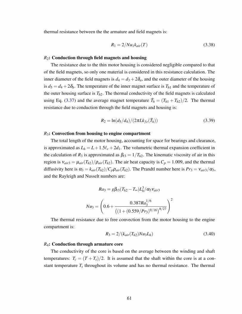
thermal resistance between the the armature and field magnets is:
R1 = 2/Nu1kair(T ) (3.38)
R2: Conduction through field magnets and housingThe resistance due to the thin motor housing is considered negligible compared to that
of the field magnets, so only one material is considered in this resistance calculation. Theinner diameter of the field magnets is d4 = d3 +2δa, and the outer diameter of the housingis d5 = d4 +2δh. The temperature of the inner magnet surface is Th1 and the temperature ofthe outer housing surface is Th2. The thermal conductivity of the field magnets is calculatedusing Eq. (3.37) and the average magnet temperature Th = (Th1 + Th2)/2. The thermalresistance due to conduction through the field magnets and housing is:
R2 = ln(d5/d4)/(2πLk f e(Th)) (3.39)
R3: Convection from housing to engine compartmentThe total length of the motor housing, accounting for space for bearings and clearance,
is approximated as Lh = L+1.5`c +2d1. The volumetric thermal expansion coefficient inthe calculation of R3 is approximated as βt3 = 1/Th2. The kinematic viscosity of air in thisregion is νair3 = µair(Th2)/ρair(Th2). The air heat capacity is Cp = 1.009, and the thermaldiffusivity here is α3 = kair(Th2)/Cpρair(Th2). The Prandtl number here is Pr3 = νair3/α3,and the Rayleigh and Nusselt numbers are:
Ra3 = gβt3(Th2−T∞)L3h/α3νair3
Nu3 =
(0.6+
0.387Ra1/63(
(1+(0.559/Pr3)9/16)8/27
)2
The thermal resistance due to free convection from the motor housing to the enginecompartment is:
R3 = 2/(kair(Th2)Nu3Lh) (3.40)
R4: Conduction through armature coreThe conductivity of the core is based on the average between the winding and shaft
temperatures: Tc = (T + Ts)/2. It is assumed that the shaft within the core is at a con-stant temperature Ts throughout its volume and has no thermal resistance. The thermal
61
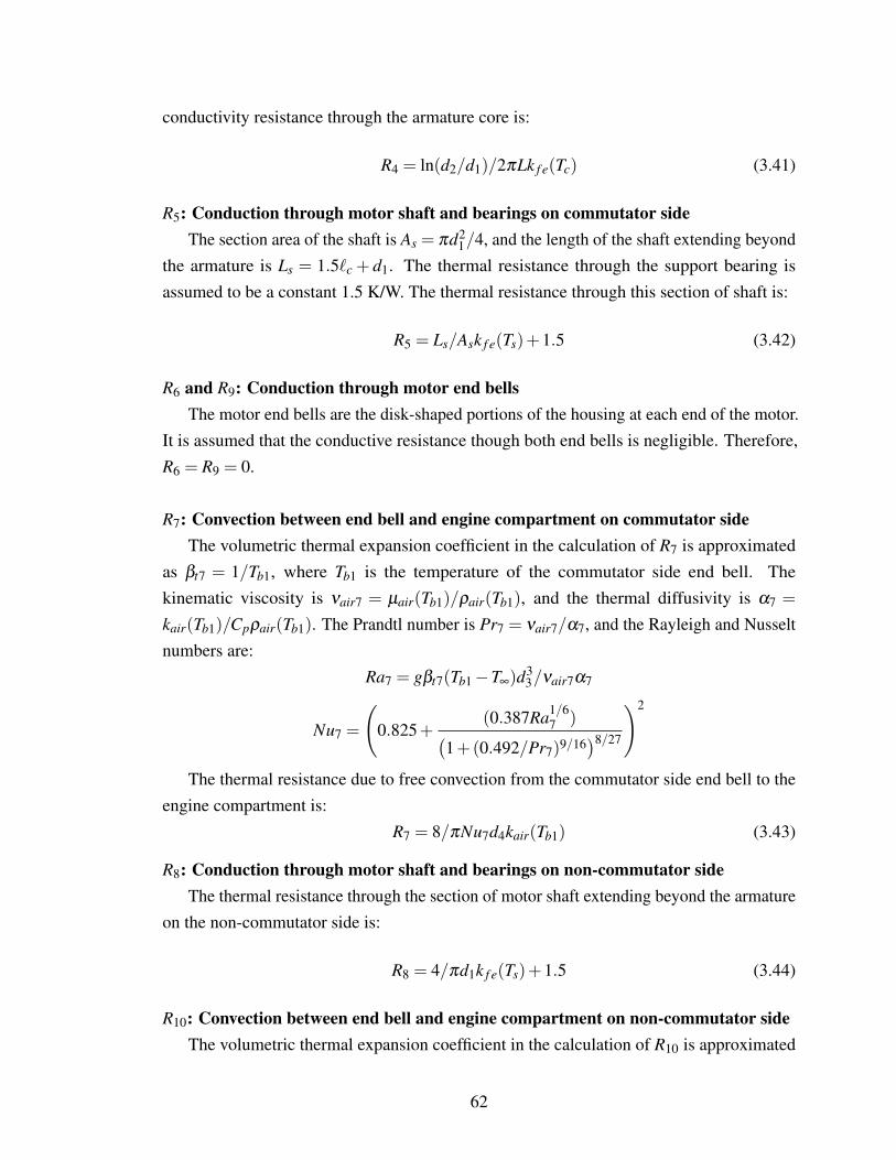
conductivity resistance through the armature core is:
R4 = ln(d2/d1)/2πLk f e(Tc) (3.41)
R5: Conduction through motor shaft and bearings on commutator sideThe section area of the shaft is As = πd2
1/4, and the length of the shaft extending beyondthe armature is Ls = 1.5`c + d1. The thermal resistance through the support bearing isassumed to be a constant 1.5 K/W. The thermal resistance through this section of shaft is:
R5 = Ls/Ask f e(Ts)+1.5 (3.42)
R6 and R9: Conduction through motor end bellsThe motor end bells are the disk-shaped portions of the housing at each end of the motor.
It is assumed that the conductive resistance though both end bells is negligible. Therefore,R6 = R9 = 0.
R7: Convection between end bell and engine compartment on commutator sideThe volumetric thermal expansion coefficient in the calculation of R7 is approximated
as βt7 = 1/Tb1, where Tb1 is the temperature of the commutator side end bell. Thekinematic viscosity is νair7 = µair(Tb1)/ρair(Tb1), and the thermal diffusivity is α7 =kair(Tb1)/Cpρair(Tb1). The Prandtl number is Pr7 = νair7/α7, and the Rayleigh and Nusseltnumbers are:
Ra7 = gβt7(Tb1−T∞)d33/νair7α7
Nu7 =
(0.825+
(0.387Ra1/67 )(
1+(0.492/Pr7)9/16)8/27
)2
The thermal resistance due to free convection from the commutator side end bell to theengine compartment is:
R7 = 8/πNu7d4kair(Tb1) (3.43)
R8: Conduction through motor shaft and bearings on non-commutator sideThe thermal resistance through the section of motor shaft extending beyond the armature
on the non-commutator side is:
R8 = 4/πd1k f e(Ts)+1.5 (3.44)
R10: Convection between end bell and engine compartment on non-commutator sideThe volumetric thermal expansion coefficient in the calculation of R10 is approximated
62
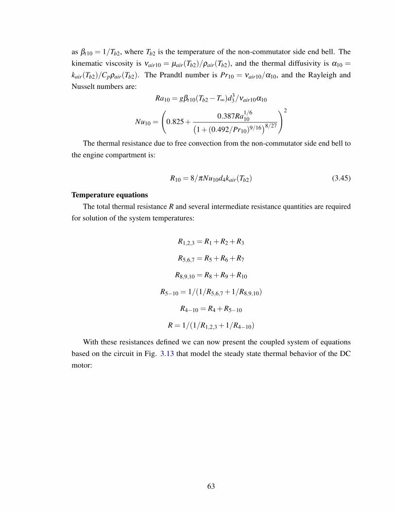
as βt10 = 1/Tb2, where Tb2 is the temperature of the non-commutator side end bell. Thekinematic viscosity is νair10 = µair(Tb2)/ρair(Tb2), and the thermal diffusivity is α10 =kair(Tb2)/Cpρair(Tb2). The Prandtl number is Pr10 = νair10/α10, and the Rayleigh andNusselt numbers are:
Ra10 = gβt10(Tb2−T∞)d33/νair10α10
Nu10 =
(0.825+
0.387Ra1/610(
1+(0.492/Pr10)9/16)8/27
)2
The thermal resistance due to free convection from the non-commutator side end bell tothe engine compartment is:
R10 = 8/πNu10d4kair(Tb2) (3.45)
Temperature equationsThe total thermal resistance R and several intermediate resistance quantities are required
for solution of the system temperatures:
R1,2,3 = R1 +R2 +R3
R5,6,7 = R5 +R6 +R7
R8,9,10 = R8 +R9 +R10
R5−10 = 1/(1/R5,6,7 +1/R8,9,10)
R4−10 = R4 +R5−10
R = 1/(1/R1,2,3 +1/R4−10)
With these resistances defined we can now present the coupled system of equationsbased on the circuit in Fig. 3.13 that model the steady state thermal behavior of the DCmotor:
63
T = T∞ +RS (3.46a)
4T = T −T∞ (3.46b)
qp1 = 4T/R1,2,3 (3.46c)
qp2 = 4T/R4−10 (3.46d)
Th1 = T −qp1R1 (3.46e)
Th2 = Th1−qp1R2 (3.46f)
Ts = T −qp2R4 (3.46g)
qp3 = (Ts−T∞)/R5,6,7 (3.46h)
qp4 = (Ts−T∞)/R8,9,10 (3.46i)
Tb1 = Ts−qp3(R5 +R6) (3.46j)
Tb2 = Ts−qp4(R8 +R9) (3.46k)
where 4T is the temperature drop between the armature windings and the engine com-partment, and qp1,qp2,qp3, and qp4 are heat flows through circuit paths formed by R1,2,3,R4−10, R5,6,7, and R8,9,10, respectively. Since many thermal resistance values depend ontemperature values the system of equations is coupled, and must be solved using an iterativetechnique. A least squares approach has been found to be more successful at solving thissystem than nonlinear Gauss-Seidel or Newton’s method.
3.5.4 Motor Current Analysis
The motor current model predicts the current through the motor armature I given thearmature temperature T , required motor shaft torque τ , and motor geometry. The magneticfield depends on temperature and is approximated using the formula:
B = Br (1−0.0017(T −293))
where Br is the remanent magnetic flux density (assumed constant). The magnetic flux isφ = π(d2 +d3)LB/2, and the total number of conductors in the magnetic field is Z = 2nt .The calculation for the number of winding turns nt was given in Section 3.5.3. The motorcurrent is:
I = τπ/φ pZ (3.47)
64
3.5.5 Motor Speed Analysis
The objective of this analysis is to compute the motor speed ω given the motor current I andarmature temperature T . The model accounts for both the electrical resistance through thearmature windings and the voltage drop across the commutator. The resistance through thewindings is Ra = 4ρ`/πd2. Recall that Eq. (3.33) is used to model the dependence of copperresistivity on temperature. The length ` is computed according to the formulae in Section3.5.3. The back emf, i.e., voltage generated due to motor rotation that opposes sourcevoltage, is E = RaI. The voltage drop across the commutator consists of two compoents:
4Vc =4Vc1 +4Vc2
A model for each component was developed based on empirical data from [78]:
4Vc1 = 0.8692−0.6458 · e−0.8207ρI
4Vc2 = 1.0037−0.5912 · e−1.32ρI
where ρI = I/Ab is the current density at the commutator/brush interface, and Ab = πdc`c/2is the brush contact area. It is assumed here that the commutator diameter is proportional toarmature diameter: dc = d3/2. The motor speed is:
ω = 2π(V −4Vc− IRa)/φZp (3.48)
3.5.6 Torque and Pressure Analysis
The analysis presented in this section computes the torque τ required to drive the pump atthe specified motor speed ω and pump flow rate Q. The analysis also computed the pressuredifferential P across the pump inlet and outlet. The equations here are based on the modelpresented in [144], and much of the notation has been retained. Some modifications havebeen made to smooth analysis responses so that optimization can be performed more easily.Note that many of the terms used in the following equations have been defined in Tables 3.4and 3.5.
The impeller blade tip speed at the outlet is u2 = ωD2/2, and the radial fluid velocityrelative to the impeller is Wm2 = Q/πD2b. The fluid velocity leaving the impeller in thedirection of the blade is W2 = Wm2/cos(β2). The Wiesner slip coefficient is:
σ = 1−√
sin(π/2−β2)n0.7
B
65

The tangential velocity of the fluid leaving the impeller relative to a fixed coordinatesystem is Ct2 = u2σ −Wm2 tan(β2), and the pump theoretical head is:
Hth = u2Ct2/g
where g is the acceleration of gravity. The disk friction loss is
DFH =CDFρcω3(D2/2)5
Q
The fluid velocity at the inlet in the radial direction with respect to a fixed coordinatesystem is C1 = 4Q/(D2
1−D2s )π . It is possible to configure a pump such that the drive
shaft does not impede flow at the inlet. This is assumed to be the case, and thereforeDs = 0. The impeller blade tip speed at the inlet is u1 = ωD1/2, and the velocity of the fluidentering the impeller in the direction of the blade is W1 =
√C2
1 +u21. The inlet flow angle is
βF1 = tan−1(u1/C1). Several intermediate values must be determined to calculate the skinfriction head loss:
βs1 = 2βF1−β1
T1 =
√cos2(βF1)− cos(β1)cos(βs1)
cos(βs1)
T2 =
T1 if Rt1 ≥ 0−T1 if Rt1 < 0
Rt1 = cos(βF1)/cos(βs1)
xL1 = Rt1−T2
DQIN12 =W 2
12gx2
L1
(1− xL1 cos(βF1)
cos(β1)
)2
DH12 =bD2π cos(β2)
nB(b+πD2 cos(β2)/nB)
The skin friction head loss is:
DQSF12 =CSF(D2−D1)(W2 +W1)2
8gcos(β2)DH12
The impeller diffusion loss as presented in [144] is computed differently depending onthe ratio W1/W2. This introduces a discontinuity that can hinder optimization efforts. After
66
adding an exponential transition function this loss term is:
DQdif =W 2
1
8g(1+ e4(1.4−W1/W2))
The fluid velocity approaching the pump volute is:
C3 =
√(Ct2d2
d3
)2
+(
Qπd3b3
)2
The curved diffuser leading to the pump outlet as shown in Fig. 3.12 is the pump volute.The volute throat velocity is:
CQ3 =Q
πd3b3 cos(β3)
The volute head loss is:
DQIN23 =
D23 if D23 ≥ 00 if D23 < 0
where D23 = Cin(C23−C2
Q3)/2g. The diffuser skin friction loss is:
DQSF34 = CSF(d3−d1)(CQ3 +C1)2
8gcos(β3)b3d3π cos(β3)
b3nV +d3π cos(β3)
The diffuser expansion loss term in [144] is calculated differently depending on thevalue of CQ3/C1. Another transition curve is defined here to eliminate the discontinuity:
ϕQVD =1
1+ e4(1.4−CQ3/C1)
The diffuser expansion loss is:
DQVD =
D24 if D24 ≥ 00 if D24 < 0
where:
D24 =(CVD +ϕQVD/4)C2
Q3−C21φQVD/2
2g
The actual head developed by the pump is:
67
Hac = Hth−DQIN12−DQSF12
−DQIN23−DQdif−DQSF34−DQVD
The pressure differential and the shaft torque can now be computed:
P = Hacρcg (3.49)
τ =ρgQ
ω(Hth +DFH) (3.50)
3.5.7 Optimization Results
The solution to Problem (3.30) obtained using the mesh adaptive direct search algorithm andthe IDF formulation is presented in Table 3.6. The minimal power consumption is 140 W, asubstantial improvement over traditional water pumps of similar capacity, which consumenearly 300 W continuously [77]. Numerous starting points and algorithm parameters weretested, and the solution presented is the best that has been obtained. It is unknown whetherthis is the global solution. The stochastic nature of the optimization algorithm makes exactreplication difficult, but similar results have been obtained from multiple starting points.Gradient-based algorithms have failed to find a feasible solution thus far.
Table 3.6 Optimization results for the electric water pump design problem
Optimal pump designx1 = d 8.4 (mm)x2 = d2 76.6 (mm)x3 = d3 146 (mm)x4 = L 145 (mm)x5 = `c 55.4 (mm)x6 = D2 58.8 (mm)x7 = b 28.5 (mm)x8 = β1 0.793 (rad)x9 = β2 1.22 (rad)x10 = β3 0.913 (rad)
68

3.6 Concluding Comments
This chapter introduced several original system design examples, ranging from air flowsensor design to the design of a commercial aircraft fleet. Each example, with the exceptionof the aircraft family problem, was presented with enough detail for replication. Not onlydoes this enable verification of results, but provides a small library of system design examplesfor use in other investigations. These examples are used throughout this dissertation toillustrate important concepts and to demonstrate partitioning and coordination techniques.The air flow sensor design problem and the turbine blade design problem are used inSection 4.2.3 to illustrate the influence of coupling strength on solution difficulty for twodifferent single-level formulations. These two examples are useful for this for this studysince their coupling strength can be varied easily. The ATC formulation is demonstratedusing the aircraft family problem in Section 4.3.3, and a parametric study on ATC algorithmparameters using this example is presented. The air flow sensor problem is also used to helpexplain the ALC formulation in Section 4.3.5. The electric water pump design problemis used for comparing partitioning and coordination decision techniques in Chapters 5and 6. An evolutionary algorithm for making partitioning and coordination decisions forlarger systems is presented in Chapter 6, and illustrated using an eight-bar version of thegeneralized truss design problem.
An electric vehicle design problem was developed to illustrate the applicability ofoptimal partitioning and coordination decision techniques to a larger and more involvedsystem design problem. Detailed description of this example problem is reserved untilChapter 8.
The following chapter introduces several important single and multi-level formulationsfor system design optimization. This dissertation emphasizes a class of multi-level formula-tions suitable for quasiseparable problems that have established convergence proofs, suchas ATC and ALC. The review of single-level formulations helps establish concepts that areimportant to multi-level formulations.
69
Chapter 4
System Design Optimization Formulations
Solution of a system design problem using decomposition-based design optimization re-quires the formulation of one or more optimization problems. The numerous formulationsthat have been proposed can be classified according to several different criteria. One im-portant distinction is whether a formulation is single-level or multi-level. Single-levelformulations comprise a single optimization problem. Analysis functions may be distributedand temporarily decoupled, but a single optimization algorithm guides the entire systemoptimization process. Multi-level methods utilize distributed optimization—a separateoptimization problem is defined for each subproblem.
This chapter reviews several important single and multi-level formulations. The single-level review provides important background for understanding multi-level formulations. Thepartitioning and decision model employed in subsequent chapters assume that a particularclass of multi-level formulations is used. The formulation used in decomposition-baseddesign optimization is a defining feature of an implementation. The type of formulationemployed dictates what types of partitions, linking structures, and coordination algorithmsmay be used. Some formulations are better suited for problems with certain structures.Convergence proofs exist for a handful of formulations.
4.1 Single-Level Formulations
Cramer et al. presented three single level formulations and provided guidance and predictionsregarding application and performance of these formulations [35]. In these single-levelformulations, all decision making is centralized and performed by a single optimizationalgorithm. This implicitly guarantees shared design variable consistency. Coupling variableconsistency can be enforced using either a system analysis algorithm, or auxiliary equalityconstraints. Single-level formulations can be effective at dealing with systems possessingstrong interactions, but are not well suited for problems of large dimension, where multilevelformulations may be preferred [5, 7]. Balling and Sobieski provided a review of single-
70
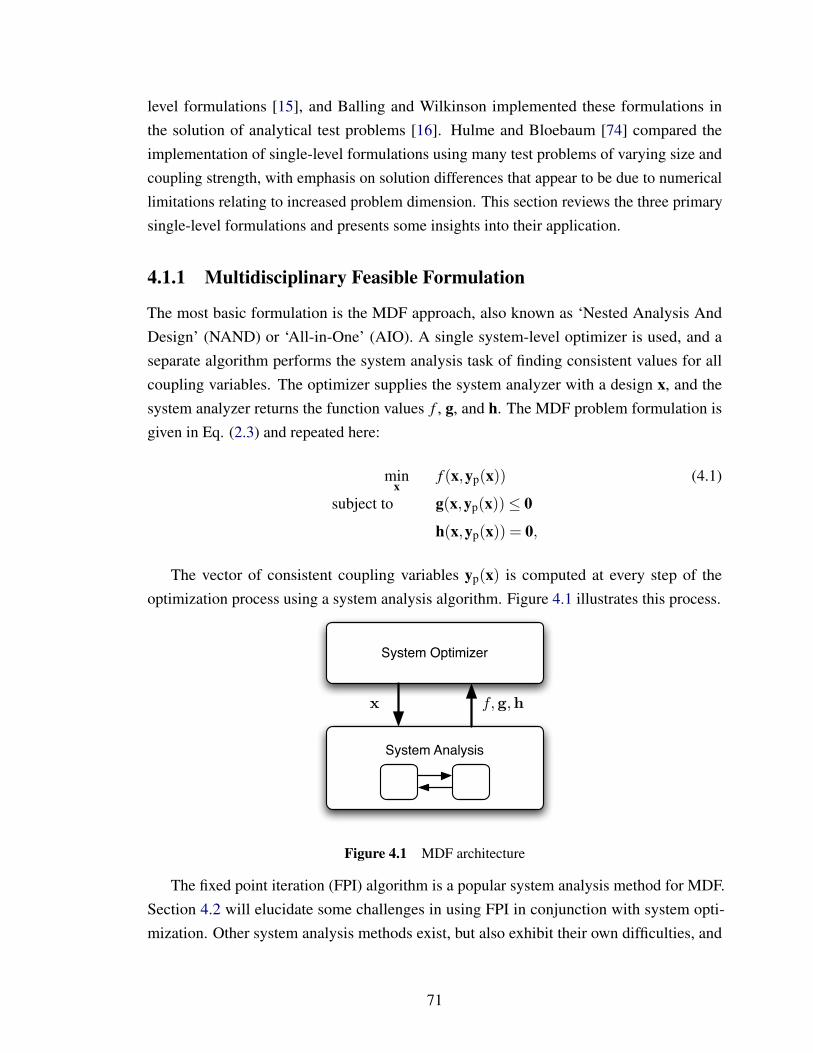
level formulations [15], and Balling and Wilkinson implemented these formulations inthe solution of analytical test problems [16]. Hulme and Bloebaum [74] compared theimplementation of single-level formulations using many test problems of varying size andcoupling strength, with emphasis on solution differences that appear to be due to numericallimitations relating to increased problem dimension. This section reviews the three primarysingle-level formulations and presents some insights into their application.
4.1.1 Multidisciplinary Feasible Formulation
The most basic formulation is the MDF approach, also known as ‘Nested Analysis AndDesign’ (NAND) or ‘All-in-One’ (AIO). A single system-level optimizer is used, and aseparate algorithm performs the system analysis task of finding consistent values for allcoupling variables. The optimizer supplies the system analyzer with a design x, and thesystem analyzer returns the function values f , g, and h. The MDF problem formulation isgiven in Eq. (2.3) and repeated here:
minx
f (x,yp(x)) (4.1)
subject to g(x,yp(x))≤ 0
h(x,yp(x)) = 0,
The vector of consistent coupling variables yp(x) is computed at every step of theoptimization process using a system analysis algorithm. Figure 4.1 illustrates this process.
System Optimizer
System Analysis
x f,g,h
Figure 4.1 MDF architecture
The fixed point iteration (FPI) algorithm is a popular system analysis method for MDF.Section 4.2 will elucidate some challenges in using FPI in conjunction with system opti-mization. Other system analysis methods exist, but also exhibit their own difficulties, and
71
will not be discussed in this chapter. A design optimization strategy is classified as MDF ifa complete system analysis is performed for every optimization iteration. The analysis is“nested” within the design. The optimizer is responsible to find the optimal design x∗ (thedesign solution), while the system analyzer is responsible to find yp(x) (the system analysissolution).
This approach may be desirable if the subsystems are weakly coupled (fast systemanalysis convergence), and if the subsystem analyses are not computationally expensive. Inaddition, MDF eases the incorporation of legacy analysis tools. If a design organizationalready performs a complete analysis before making a design decision, MDF is a natural fit.
Although the merits of MDF are notable, its shortcomings must be clearly understood.MDF is dependent upon the effectiveness of the system analyzer. If the analyzer doesnot converge at any point in the process, the optimizer may fail. The nested analysis andoptimization process required by MDF can be computationally inefficient, and this motivatesapproaches that eliminate the need for repeated system analysis [128]. In addition, typicalMDF implementations cannot exploit the potential coarse-grained parallelism of distinctsubsystem analyses. MDF has been aptly termed a ‘brute force’ approach [25].
4.1.2 Individual Disciplinary Feasible Formulation
In the IDF formulation, an analyzer for each subsystem is employed and a single system-leveloptimizer is used, but the optimizer, rather than a system analysis algorithm, coordinatesthe interactions between the subsystem analyses. The IDF architecture is illustrated in Fig.4.2 using a two-element example system. The first analysis function computes the designconstraints g1 and h1, as well as the coupling variable y21. The second analysis functioncomputes the objective function in addition to a coupling variable and a set of designconstraints. The optimizer chooses values for both design and coupling variables: systemanalysis and design are performed simultaneously. Since the system optimizer provides allinputs required for all subsystems concurrently, subsystem analyses may be executed inparallel.
The IDF formulation is given in Eq. (4.2). It differs from the MDF formulation in thatthe decision variable vector includes both design variables x and coupling variables y, whileauxiliary constraints haux are added to ensure system consistency. This approach eliminatesthe need to solve for yp(x) at each optimization iteration. In cases where solving the system
72

System Optimizer
x!1,xs1,y12 x!2,xs2,y21
a1 a2
g1,h1,y21 f,g2,h2,y12
Figure 4.2 IDF architecture
analysis equations is difficult, IDF can offer great benefit.
minx=[x`,xs],y
f (x,y) (4.2)
subject to g(x,y)≤ 0
h(x,y) = 0
haux(x,y) = y−a(x,y)S = 0
IDF facilitates coarse-grained parallelism, improves convergence properties, and drivesthe design toward better solutions if multiple analysis solutions exist. If the solution processis interrupted, the intermediate design may not be consistent or feasible. In contrast, aninterrupted MDF solution will yield a consistent, but potentially infeasible, design. SinceIDF does not require the frequently expensive task of achieving system consistency whenfar from the solution, the optimization algorithm can trace a more efficient path toward thesolution and computational expense is reduced through the elimination of repeated systemanalysis steps [3].
IDF is more centralized than MDF, and the dimension of the optimization problem isincreased since coupling variables are made decision variables. This increase in dimensioncan reduce numerical solution accuracy when the problem size is large, as evident inthe results presented by Hulme and Bloebaum [74]. MDF may be preferable when thedimension of y is much larger than the dimension of x [3, 66]. Furthermore, auxiliaryequality constraints can introduce numerical solution difficulties [3, 138].
Balling and Sobieski proposed a hybrid approach to handling coupling variable consis-tency [15]. In MDF the task of satisfying coupling variable consistency is nested within theoptimization problem. In IDF it is part of the optimization problem. A hybrid approach
73
satisfies some consistency constraints using the optimization algorithm, and the rest usingan approach nested within the algorithm. If all feedback coupling relationships are handledusing auxiliary equality constraints, then the remaining feedforward relationships can be sat-isfied by simply executing the analysis functions in sequence and utilizing the most recentlycomputed coupling variable values. An implementation of this idea was demonstrated inSection 1.4.
Section 4.2.2 will show that using the IDF formulation can help to find superior solutionsthat are hidden to MDF implementations, and Section 4.2.3 demonstrates that IDF results inimproved computational efficiency for strongly coupled problems (as predicted in [35]). If ahigh level of centralization is acceptable, IDF may be an ideal design strategy.
4.1.3 All-at-Once Formulation
The All-at-Once (AAO) formulation confers additional tasks to the optimization algorithmbeyond those for the IDF formulation. In IDF the optimization algorithm solves the systemanalysis equations, but relies on analysis algorithms within each analysis function to solve theassociated governing equations. For example, an analysis function that evaluates structuralintegrity of a component may use the finite element method [93] to solve the governingelasticity equations and compute the analysis function outputs. The AAO formulationuses the optimization algorithm instead to solve these governing equations, eliminatingthe need for the analysis algorithm within each analysis function. The vector of statevariables (s) is added to the decision variable set, and the governing equations are cast as anadditional set of auxiliary equality constraints. State variables quantify the state of a system;examples include velocity fields in computational fluid dynamics, strain fields in structuralfinite element analysis, and component velocities or accelerations in multibody dynamics.Governing equations are satisfied when the associated residuals are zero. The AAO processis illustrated in Fig. 4.3 using a simple example system.
The formulation of the AAO approach is given in Eq. (4.3). Auxiliary equality con-straints ensure zero residuals at problem convergence, and the decision variables include xand s. The evaluation function e(x,s) computes the residuals as well as design constraintand objective values. The selection matrix Sw extracts the evaluation function outputs thatare the evaluation function residuals w.
74
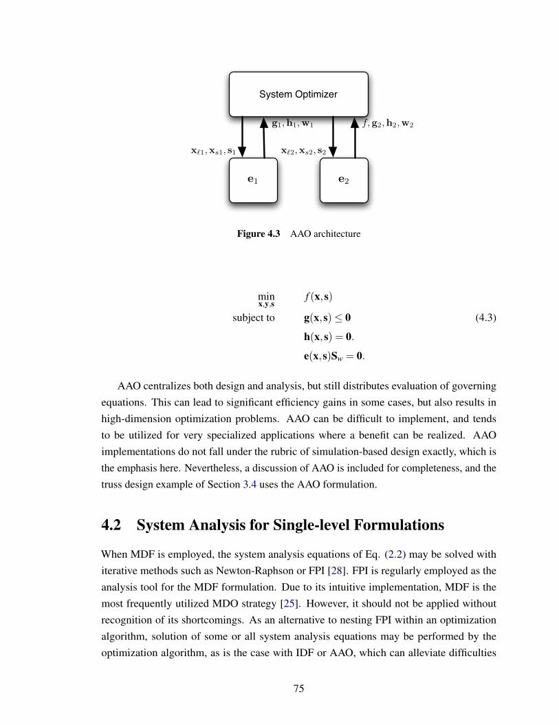
System Optimizer
x!1,xs1, s1 x!2,xs2, s2
e1 e2
g1,h1,w1 f,g2,h2,w2
Figure 4.3 AAO architecture
minx,y,s
f (x,s)
subject to g(x,s)≤ 0 (4.3)
h(x,s) = 0.
e(x,s)Sw = 0.
AAO centralizes both design and analysis, but still distributes evaluation of governingequations. This can lead to significant efficiency gains in some cases, but also results inhigh-dimension optimization problems. AAO can be difficult to implement, and tendsto be utilized for very specialized applications where a benefit can be realized. AAOimplementations do not fall under the rubric of simulation-based design exactly, which isthe emphasis here. Nevertheless, a discussion of AAO is included for completeness, and thetruss design example of Section 3.4 uses the AAO formulation.
4.2 System Analysis for Single-level Formulations
When MDF is employed, the system analysis equations of Eq. (2.2) may be solved withiterative methods such as Newton-Raphson or FPI [28]. FPI is regularly employed as theanalysis tool for the MDF formulation. Due to its intuitive implementation, MDF is themost frequently utilized MDO strategy [25]. However, it should not be applied withoutrecognition of its shortcomings. As an alternative to nesting FPI within an optimizationalgorithm, solution of some or all system analysis equations may be performed by theoptimization algorithm, as is the case with IDF or AAO, which can alleviate difficulties
75
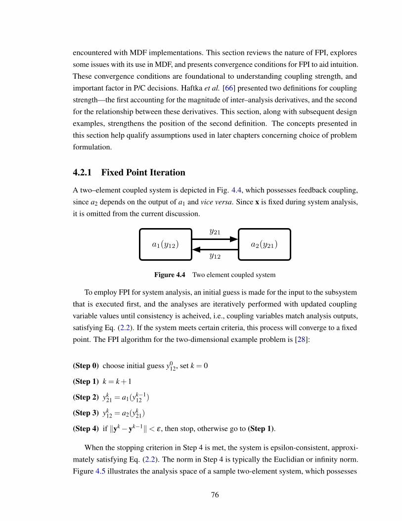
encountered with MDF implementations. This section reviews the nature of FPI, exploressome issues with its use in MDF, and presents convergence conditions for FPI to aid intuition.These convergence conditions are foundational to understanding coupling strength, andimportant factor in P/C decisions. Haftka et al. [66] presented two definitions for couplingstrength—the first accounting for the magnitude of inter–analysis derivatives, and the secondfor the relationship between these derivatives. This section, along with subsequent designexamples, strengthens the position of the second definition. The concepts presented inthis section help qualify assumptions used in later chapters concerning choice of problemformulation.
4.2.1 Fixed Point Iteration
A two–element coupled system is depicted in Fig. 4.4, which possesses feedback coupling,since a2 depends on the output of a1 and vice versa. Since x is fixed during system analysis,it is omitted from the current discussion.
a1(y12) a2(y21)
y21
y12
Figure 4.4 Two element coupled system
To employ FPI for system analysis, an initial guess is made for the input to the subsystemthat is executed first, and the analyses are iteratively performed with updated couplingvariable values until consistency is acheived, i.e., coupling variables match analysis outputs,satisfying Eq. (2.2). If the system meets certain criteria, this process will converge to a fixedpoint. The FPI algorithm for the two-dimensional example problem is [28]:
(Step 0) choose initial guess y012, set k = 0
(Step 1) k = k +1
(Step 2) yk21 = a1(yk−1
12 )
(Step 3) yk12 = a2(yk
21)
(Step 4) if ‖yk−yk−1‖< ε , then stop, otherwise go to (Step 1).
When the stopping criterion in Step 4 is met, the system is epsilon-consistent, approxi-mately satisfying Eq. (2.2). The norm in Step 4 is typically the Euclidian or infinity norm.Figure 4.5 illustrates the analysis space of a sample two-element system, which possesses
76
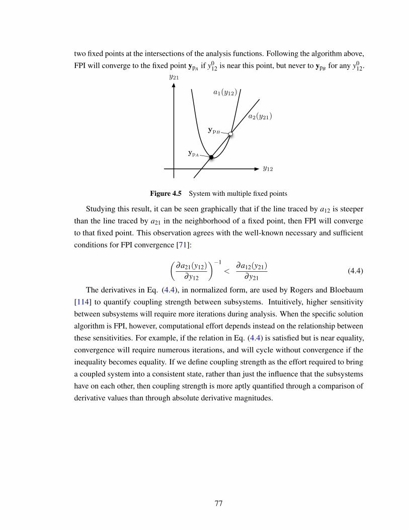
two fixed points at the intersections of the analysis functions. Following the algorithm above,FPI will converge to the fixed point ypA if y0
12 is near this point, but never to ypB for any y012.
y12
y21
ypA
a12(y21)
a21(y12)
ypB
a1(y12)
a2(y21)
Figure 4.5 System with multiple fixed points
Studying this result, it can be seen graphically that if the line traced by a12 is steeperthan the line traced by a21 in the neighborhood of a fixed point, then FPI will convergeto that fixed point. This observation agrees with the well-known necessary and sufficientconditions for FPI convergence [71]:(
∂a21(y12)∂y12
)−1
<∂a12(y21)
∂y21(4.4)
The derivatives in Eq. (4.4), in normalized form, are used by Rogers and Bloebaum[114] to quantify coupling strength between subsystems. Intuitively, higher sensitivitybetween subsystems will require more iterations during analysis. When the specific solutionalgorithm is FPI, however, computational effort depends instead on the relationship betweenthese sensitivities. For example, if the relation in Eq. (4.4) is satisfied but is near equality,convergence will require numerous iterations, and will cycle without convergence if theinequality becomes equality. If we define coupling strength as the effort required to bringa coupled system into a consistent state, rather than just the influence that the subsystemshave on each other, then coupling strength is more aptly quantified through a comparison ofderivative values than through absolute derivative magnitudes.
77
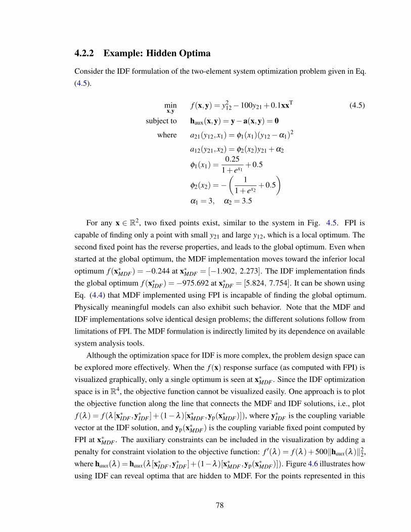
4.2.2 Example: Hidden Optima
Consider the IDF formulation of the two-element system optimization problem given in Eq.(4.5).
minx,y
f (x,y) = y212−100y21 +0.1xxT (4.5)
subject to haux(x,y) = y−a(x,y) = 0
where a21(y12,x1) = φ1(x1)(y12−α1)2
a12(y21,x2) = φ2(x2)y21 +α2
φ1(x1) =0.25
1+ ex1+0.5
φ2(x2) =−(
11+ ex2
+0.5)
α1 = 3, α2 = 3.5
For any x ∈ R2, two fixed points exist, similar to the system in Fig. 4.5. FPI iscapable of finding only a point with small y21 and large y12, which is a local optimum. Thesecond fixed point has the reverse properties, and leads to the global optimum. Even whenstarted at the global optimum, the MDF implementation moves toward the inferior localoptimum f (x∗MDF) =−0.244 at x∗MDF = [−1.902, 2.273]. The IDF implementation findsthe global optimum f (x∗IDF) =−975.692 at x∗IDF = [5.824, 7.754]. It can be shown usingEq. (4.4) that MDF implemented using FPI is incapable of finding the global optimum.Physically meaningful models can also exhibit such behavior. Note that the MDF andIDF implementations solve identical design problems; the different solutions follow fromlimitations of FPI. The MDF formulation is indirectly limited by its dependence on availablesystem analysis tools.
Although the optimization space for IDF is more complex, the problem design space canbe explored more effectively. When the f (x) response surface (as computed with FPI) isvisualized graphically, only a single optimum is seen at x∗MDF . Since the IDF optimizationspace is in R4, the objective function cannot be visualized easily. One approach is to plotthe objective function along the line that connects the MDF and IDF solutions, i.e., plotf (λ ) = f (λ [x∗IDF ,y∗IDF ]+ (1−λ )[x∗MDF ,yp(x∗MDF)]), where y∗IDF is the coupling variablevector at the IDF solution, and yp(x∗MDF) is the coupling variable fixed point computed byFPI at x∗MDF . The auxiliary constraints can be included in the visualization by adding apenalty for constraint violation to the objective function: f ′(λ ) = f (λ )+500‖haux(λ )‖2
2,where haux(λ ) = haux(λ [x∗IDF ,y∗IDF ]+(1−λ )[x∗MDF ,yp(x∗MDF)]). Figure 4.6 illustrates howusing IDF can reveal optima that are hidden to MDF. For the points represented in this
78
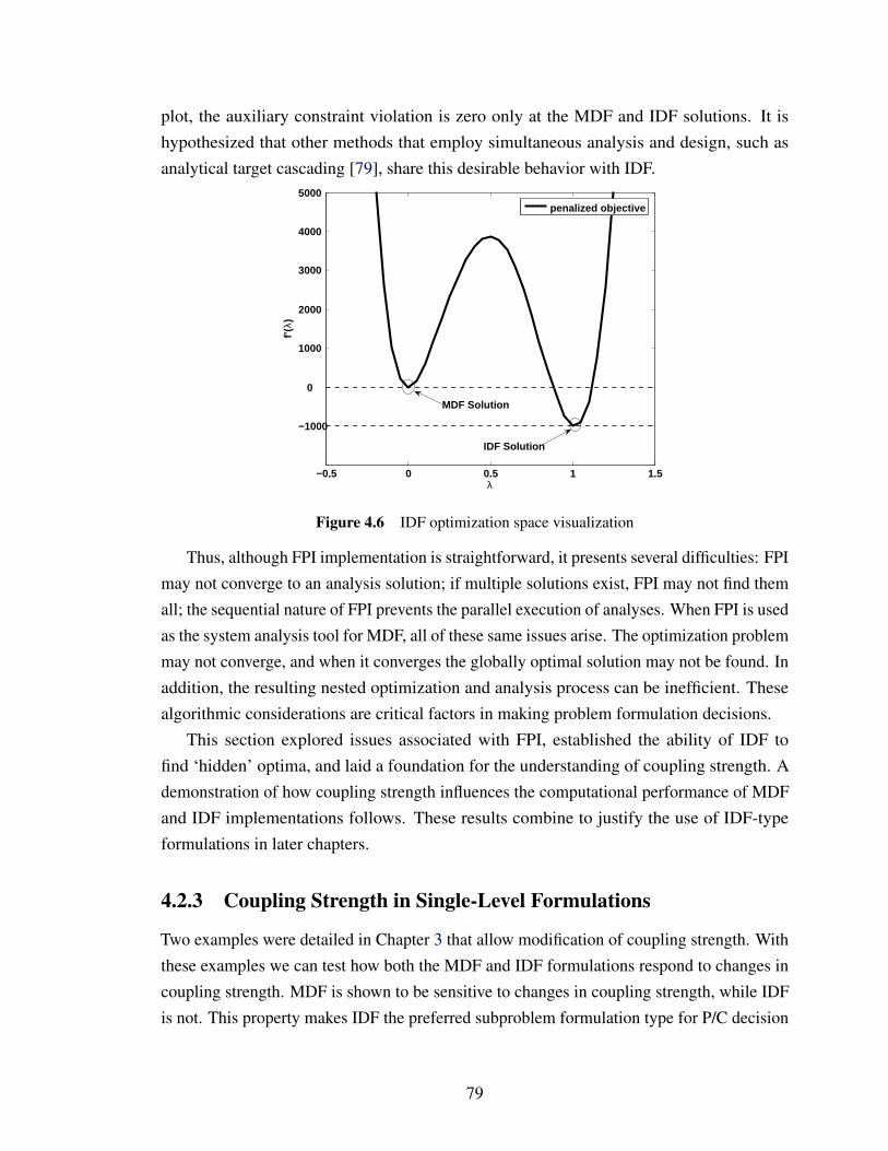
plot, the auxiliary constraint violation is zero only at the MDF and IDF solutions. It ishypothesized that other methods that employ simultaneous analysis and design, such asanalytical target cascading [79], share this desirable behavior with IDF.
−0.5 0 0.5 1 1.5
−1000
0
1000
2000
3000
4000
5000
λ
f’(λ)
penalized objective
MDF Solution
IDF Solution
Figure 4.6 IDF optimization space visualization
Thus, although FPI implementation is straightforward, it presents several difficulties: FPImay not converge to an analysis solution; if multiple solutions exist, FPI may not find themall; the sequential nature of FPI prevents the parallel execution of analyses. When FPI is usedas the system analysis tool for MDF, all of these same issues arise. The optimization problemmay not converge, and when it converges the globally optimal solution may not be found. Inaddition, the resulting nested optimization and analysis process can be inefficient. Thesealgorithmic considerations are critical factors in making problem formulation decisions.
This section explored issues associated with FPI, established the ability of IDF tofind ‘hidden’ optima, and laid a foundation for the understanding of coupling strength. Ademonstration of how coupling strength influences the computational performance of MDFand IDF implementations follows. These results combine to justify the use of IDF-typeformulations in later chapters.
4.2.3 Coupling Strength in Single-Level Formulations
Two examples were detailed in Chapter 3 that allow modification of coupling strength. Withthese examples we can test how both the MDF and IDF formulations respond to changes incoupling strength. MDF is shown to be sensitive to changes in coupling strength, while IDFis not. This property makes IDF the preferred subproblem formulation type for P/C decision
79

models presented in later chapters.
Air-flow Sensor Design Problem
The first variable coupling-strength example is the vane air-flow sensor design problemfrom Section 3.1. It consists of coupled structural and aerodynamic analyses. The couplingvariables are the stator deflection (θ ) and the drag force (F). The analysis structure isillustrated in Fig. 4.7.
SS1: Structural Analysis SS2: Aerodynamic Analysisy21 = !
y12 = F
x1 = ! x2 = [!, w]
!(", F ) F (!, w, ")
Figure 4.7 Coupling relationship in airflow sensor analysis
The objective in this design problem is to adjust the stator geometry such that the statordeflection is as close as possible to a target deflection (θ ) for a given airspeed. MDFformulation is:
min`,w
(θ − θ)2
subject to F−Fmax ≤ 0 (4.6)`w−A = 0
Consistent values for F and θ are obtained using FPI. The exact solution can be obtainedusing monotonicity analysis (MA). The MDF solution matches the MA solution describedin Eq. (3.5). The IDF solution requires the addition of θ and F to the decision variable set,as well as auxiliary constraints on these values, as shown in Eq. (4.7). The IDF solutionalso matches the MA solution.
min`,w,θ ,F
(θ − θ)2 (4.7)
subject to F−Fmax ≤ 0`w−A = 0θ −θ(`, F) = 0F−F(`,w, θ) = 0
80
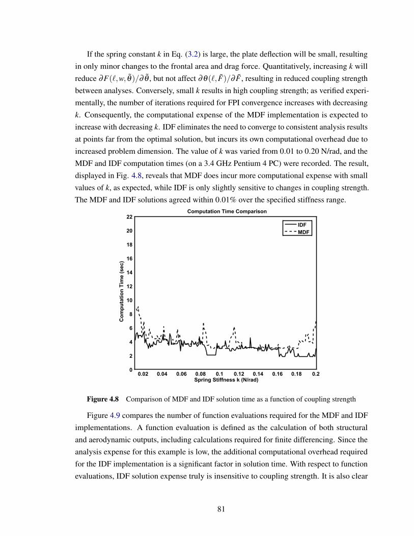
If the spring constant k in Eq. (3.2) is large, the plate deflection will be small, resultingin only minor changes to the frontal area and drag force. Quantitatively, increasing k willreduce ∂F(`,w, θ)/∂ θ , but not affect ∂θ(`, F)/∂ F , resulting in reduced coupling strengthbetween analyses. Conversely, small k results in high coupling strength; as verified experi-mentally, the number of iterations required for FPI convergence increases with decreasingk. Consequently, the computational expense of the MDF implementation is expected toincrease with decreasing k. IDF eliminates the need to converge to consistent analysis resultsat points far from the optimal solution, but incurs its own computational overhead due toincreased problem dimension. The value of k was varied from 0.01 to 0.20 N/rad, and theMDF and IDF computation times (on a 3.4 GHz Pentium 4 PC) were recorded. The result,displayed in Fig. 4.8, reveals that MDF does incur more computational expense with smallvalues of k, as expected, while IDF is only slightly sensitive to changes in coupling strength.The MDF and IDF solutions agreed within 0.01% over the specified stiffness range.
0.02 0.04 0.06 0.08 0.1 0.12 0.14 0.16 0.18 0.20
2
4
6
8
10
12
14
16
18
20
22
Spring Stiffness k (N/rad)
)ces( emiT noi ta tup
moC
Computation Time Comparison
IDFMDF
Figure 4.8 Comparison of MDF and IDF solution time as a function of coupling strength
Figure 4.9 compares the number of function evaluations required for the MDF and IDFimplementations. A function evaluation is defined as the calculation of both structuraland aerodynamic outputs, including calculations required for finite differencing. Since theanalysis expense for this example is low, the additional computational overhead requiredfor the IDF implementation is a significant factor in solution time. With respect to functionevaluations, IDF solution expense truly is insensitive to coupling strength. It is also clear
81
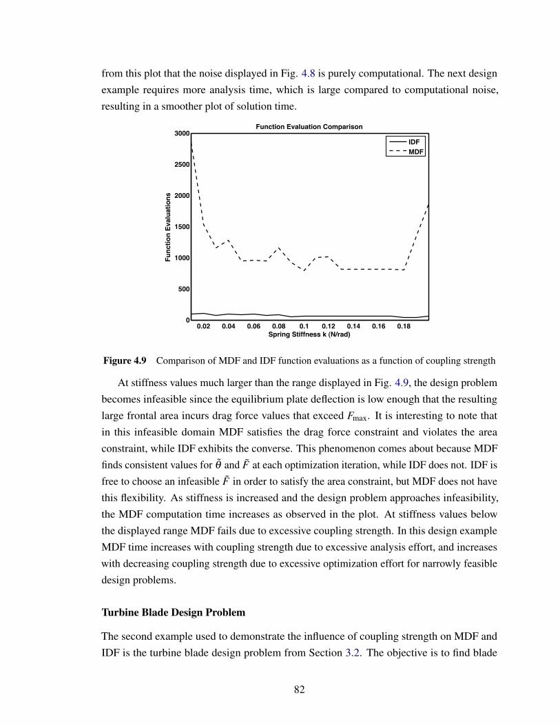
from this plot that the noise displayed in Fig. 4.8 is purely computational. The next designexample requires more analysis time, which is large compared to computational noise,resulting in a smoother plot of solution time.
0.02 0.04 0.06 0.08 0.1 0.12 0.14 0.16 0.180
500
1000
1500
2000
2500
3000
Spring Stiffness k (N/rad)
Func
tion
Eval
uatio
ns
Function Evaluation Comparison
IDFMDF
Figure 4.9 Comparison of MDF and IDF function evaluations as a function of coupling strength
At stiffness values much larger than the range displayed in Fig. 4.9, the design problembecomes infeasible since the equilibrium plate deflection is low enough that the resultinglarge frontal area incurs drag force values that exceed Fmax. It is interesting to note thatin this infeasible domain MDF satisfies the drag force constraint and violates the areaconstraint, while IDF exhibits the converse. This phenomenon comes about because MDFfinds consistent values for θ and F at each optimization iteration, while IDF does not. IDF isfree to choose an infeasible F in order to satisfy the area constraint, but MDF does not havethis flexibility. As stiffness is increased and the design problem approaches infeasibility,the MDF computation time increases as observed in the plot. At stiffness values belowthe displayed range MDF fails due to excessive coupling strength. In this design exampleMDF time increases with coupling strength due to excessive analysis effort, and increaseswith decreasing coupling strength due to excessive optimization effort for narrowly feasibledesign problems.
Turbine Blade Design Problem
The second example used to demonstrate the influence of coupling strength on MDF andIDF is the turbine blade design problem from Section 3.2. The objective is to find blade
82
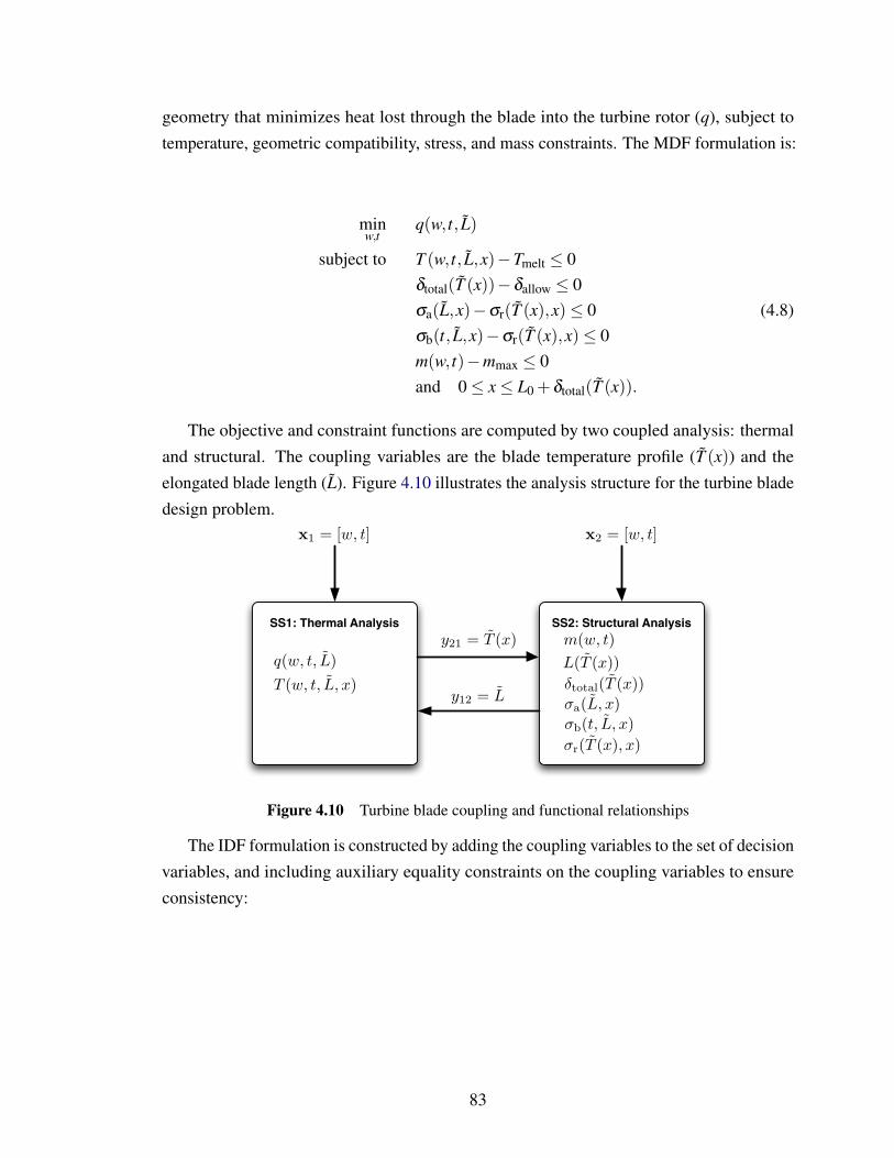
geometry that minimizes heat lost through the blade into the turbine rotor (q), subject totemperature, geometric compatibility, stress, and mass constraints. The MDF formulation is:
minw,t
q(w, t, L)
subject to T (w, t, L,x)−Tmelt ≤ 0δtotal(T (x))−δallow ≤ 0σa(L,x)−σr(T (x),x)≤ 0 (4.8)σb(t, L,x)−σr(T (x),x)≤ 0m(w, t)−mmax ≤ 0and 0≤ x≤ L0 +δtotal(T (x)).
The objective and constraint functions are computed by two coupled analysis: thermaland structural. The coupling variables are the blade temperature profile (T (x)) and theelongated blade length (L). Figure 4.10 illustrates the analysis structure for the turbine bladedesign problem.
SS1: Thermal Analysis SS2: Structural Analysism(w, t)
x1 = [w, t] x2 = [w, t]
y21 = T (x)
y12 = L
q(w, t, L)
T (w, t, L, x)
L(T (x))!total(T (x))
!b(t, L, x)!a(L, x)
!r(T (x), x)
Figure 4.10 Turbine blade coupling and functional relationships
The IDF formulation is constructed by adding the coupling variables to the set of decisionvariables, and including auxiliary equality constraints on the coupling variables to ensureconsistency:
83
minw,t,T (x),L
q(w, t, L)
subject to T (w, t, L,x)−Tmelt ≤ 0δtotal(T (x))−δallow ≤ 0σa(L,x)−σr(T (x),x)≤ 0σb(t, L,x)−σr(T (x),x)≤ 0 (4.9)m(w, t)−mmax ≤ 0T (x)−T (w, t, L,x) = 0L−L(T (x)) = 0and 0≤ x≤ L0 +δtotal(T (x)).
The function-valued coupling variable T (x) was discretized and implemented as a vector-valued coupling variable, substantially increasing the optimization problem dimension.
The computation time required for both MDF and IDF solutions was recorded over arange of coupling strength levels, varied by adjusting the modulus of elasticity E(T ). A morecompliant blade results in increased blade elongation and exposed surface area, increasingthe impact that the structural analysis results have on the thermal analysis. The E(T ) curvefrom Eq. (3.17) was multiplied by a scaling factor to produce changes in coupling strength.Figure 4.11 illustrates the dependence of MDF and IDF computation time on this modulusmultiplier, and hence the dependence on coupling strength.
As with the previous example, IDF computation time is insensitive to coupling strength,while MDF computation time increases with coupling strength. At modulus multipliervalues larger than the range illustrated, very little change in computation time was observed.In contrast to the previous example, increased stiffness does not induce infeasibility, but doesresult in very weak coupling as expected. Since design infeasibility is not a confoundingfactor as in the VAF example, MDF time monotonically increases with coupling strength. Avery stiff blade results in effectively independent analyses—only one or two FPI iterationsare required for system analysis. At modulus multiplier values smaller than the rangepresented, MDF failed due to strong coupling.
In summary, weakly coupled systems with relatively few design variables can be solvedefficiently with MDF, while strongly coupled systems require excessive iterations for theinner analysis loops of MDF. The computation time required for the IDF approach is virtuallyconstant for all levels of coupling strength investigated here. In addition to verifying thepredictions of IDF efficiency [35] for the case of a strongly coupled system, Figs. 4.8and 4.11 show a very clear relationship between coupling strength and computationalperformance.
84
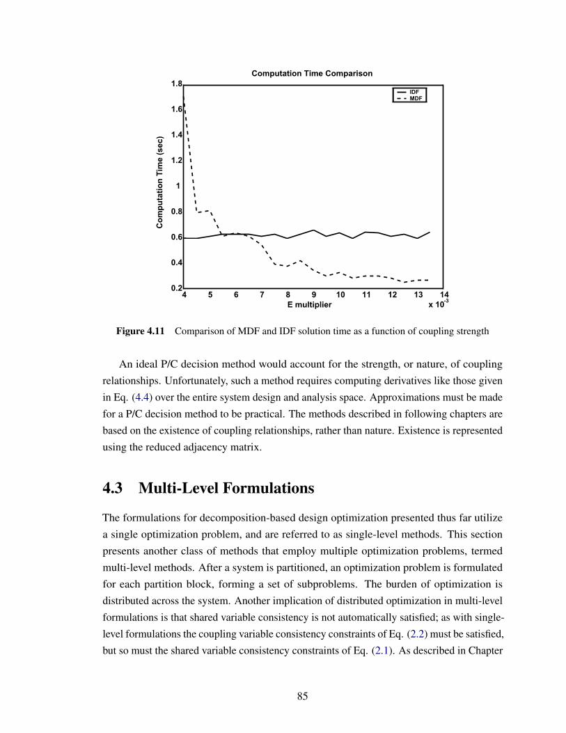
4 5 6 7 8 9 10 11 12 13 14x 10-3
0.2
0.4
0.6
0.8
1
1.2
1.4
1.6
1.8Computation Time Comparison
E multiplier
IDFMDF
Com
puta
tion
Tim
e (s
ec)
Figure 4.11 Comparison of MDF and IDF solution time as a function of coupling strength
An ideal P/C decision method would account for the strength, or nature, of couplingrelationships. Unfortunately, such a method requires computing derivatives like those givenin Eq. (4.4) over the entire system design and analysis space. Approximations must be madefor a P/C decision method to be practical. The methods described in following chapters arebased on the existence of coupling relationships, rather than nature. Existence is representedusing the reduced adjacency matrix.
4.3 Multi-Level Formulations
The formulations for decomposition-based design optimization presented thus far utilizea single optimization problem, and are referred to as single-level methods. This sectionpresents another class of methods that employ multiple optimization problems, termedmulti-level methods. After a system is partitioned, an optimization problem is formulatedfor each partition block, forming a set of subproblems. The burden of optimization isdistributed across the system. Another implication of distributed optimization in multi-levelformulations is that shared variable consistency is not automatically satisfied; as with single-level formulations the coupling variable consistency constraints of Eq. (2.2) must be satisfied,but so must the shared variable consistency constraints of Eq. (2.1). As described in Chapter
85
1, solving each of these subproblems independently will not produce a design optimal for theentire system. Interactions between subproblems must be accounted for. These interactionsare quantified using linking variables. A coordination algorithm guides the repeated solutionof subproblems toward a consistent and optimal system design. This section providesan overview of multilevel methods, and presents two multilevel formulations in detail:analytical target cascading (ATC) and augmented Lagrangian coordination (ALC).
4.3.1 Classes of Multi-Level Formulations
Important distinctions between multi-level methods relate to how subproblem solutionsare coordinated and how subproblem interactions are managed. A classical approach tocoordinating a partitioned optimization problem is to use a master optimization problemto provide information to the subproblems in a nested manner. Each subproblem is linkeddirectly to the master problem, but not directly to other subproblems. Subproblems are allat the ‘lower level’, and the master problem is at the top. This coordination approach issometimes called bi-level nested.
The first formulations for bi-level nested coordination involved linear optimizationproblems. For example, the Dantzig-Wolfe decomposition method uses a dual problemfor the master problem and a primal for each subproblem [38]. It is designed to workwith the simplex method for linear programming [37], and accommodates shared designconstraints. Wagner provided an extensive review of bi-level nested formulations [145].Several other formulations in this category have been developed, including several forgeneral nonlinear problems. Sobieski and Haftka reviewed several important multi-levelformulations, including collaborative optimization (CO) [25] and concurrent subspaceoptimization (CSSO) [126]. In CO the master problem seeks to minimize the systemobjective function by varying targets for linking variables, and requires that the subproblemvalues match corresponding targets using equality constraints. Theoretical problems withthe original CO formulation have been identified [4], and several modifications have beenproposed [41, 42, 92, 125]. CSSO takes a different approach to managing subprobleminteractions; each subproblem is solved using an approximation for other subproblems thatis constructed using global sensitivity equations (GSEs). CSSO also allows design constraintviolations at intermediate steps. In constrast, CO allows consistency constraint violation atintermediate steps, but enforce feasibility of design constraints. Bi-level system synthesis(BLISS) is another bi-level nested formulation that uses sensitivity-based subproblemapproximations when solving subproblems, and allows consistency constraint violationuntil system convergence [127]. Haftka and Watson introduced a bi-level formulation that
86
allows temporary design constraint violation, and seeks to minimize the maximum designconstraint violation until it reaches zero at convergence [67].
Bi-level formulations have proven useful, and some even have convergence proofs [67],but do have limitations. The dimension of the master problem may become unmanageableas the number of subproblems and interactions increases. Bi-level formulations force atwo-level hierarchical problem structure, which may not be ideal for certain problem types.
Another class of formulations addresses these problems by allowing more than twolevels in a problem structure, or even non-hierarchic problem structures. Penalty relaxationmethods are used to allow violation of consistency constraints until system convergence. Twoformulations belong to this class. Kim et al. introduced analytical target cascading (ATC)as a product development tool for determining consistent subsystem target values [79, 80].ATC has since been applied as a formulation for decomposition-based design optimization insimulation based design. ATC requires that subproblems are linked in a purely hierarchicalstructure. It has been shown that this structure requirement can be relaxed to accommodatenon-hierarchical links. Tosserams et al. developed a non-hierarchical generalization, calledAugmented Lagrangian Coordination (ALC) [141, 142]. Both ATC and ALC have beenproven to converge under standard nonlinear programming assumptions, such as localconvexity [106, 141]. The ATC and ALC formulations will be presented in detail below.The partitioning and coordinations decision methods presented in later chapters assume thatthe problem formulation belongs to this class.
4.3.2 Analytical Target Cascading
Analytical target cascading was developed based on needs in the automotive industry totranslate top-level product targets into detailed design specifications. It is applicable tosystems that possess hierarchical relationships. An example of the analysis relationshipsin a hierarchical system is shown in Fig. 4.12. Each element in the hierarchy computesits own local analysis responses, and may require as inputs analysis responses (couplingvariables) from lower level elements, in addition to local and shared variables. ATC canhandle systems with any number of levels.
The analysis structure displayed in Fig. 4.12 depicts unidirectional information flow.Original ATC applications possessed this structure, and initial ATC formulations did notaccount for the possibility of feedback coupling. Design variables shared between subprob-lems with a common parent element are allowed. More recent ATC formulations [7, 140]allow multidirectional coupling, and coupling between same-level elements.
The objective of the ATC process is to determine design specifications for each element
87

Level 1
Level 2
Level 3
P1 x1
x2 x3
x4 x5 x6 x7
P2 P3
P4 P5 P6 P7
y12 y13
y24 y25 y36 y37
Figure 4.12 Hierarchical system analysis structure
in the hierarchy that account for interaction so that design teams can proceed with detaildesign independently. An optimization problem is formulated for each element. Theformulation allows for a local objective and observes local design constraints. ATC allowsthe optimization algorithm to choose coupling variable values, and uses penalty functions toensure system consistency. The ATC formulation for subproblem Pi is
minxi,yi,xsCi ,yCi
fi(xi, yi)+φ(ci(xi, yi, xsCi, yCi))
subject to gi(xi, yi)≤ 0 (4.10)
hi(xi, yi) = 0
If Pi has child elements with shared design variables xsCi or coupling variables betweenthem yCi , the optimization problem for Pi sets target values for these quantities to be met bythe child elements. The vector of consistency constraints is ci, which ensures that sharedand coupling variables between child elements are consistent at ATC convergence, and thatvalues for shared and coupling variables for Pi are consistent with targets set by its parentat ATC convergence. Calculation of fi, ci, and the design constraints local to Pi (gi andhi), normally requires execution of the analysis functions belonging to Pi. ATC allows forthe possibility that more than one subproblem has an objective function. If fi is the localobjective function for subproblem Pi, then the equivalent objective function for the entiresystem is f (x, y) = ∑
Ni=1 fi(xi, yi).
The consistency constraints in the ATC subproblem formulation are relaxed using an
88

inexact penalty function φ(ci). Feasibility problems would occur during the ATC processif ci = 0 was instead cast as an equality constraint in the subproblem formulation. Severaldifferent penalty relaxation methods have been used in ATC implementations. The first wasa simple quadratic penalty function where each component of the consistency constraint ismultiplied by an importance weight, and then the squared Euclidean norm is taken of theresulting vector:
φ(ci) = ‖wi ci‖22 (4.11)
Penalty weights were typically chosen subjectively based on experience. Large weightsplace high emphasis on consistency, but struggle to achieve system optimality. In addition,large weights lead to ill conditioning of subproblems and slow convergence. If weights areset too low the system may never achieve an acceptable level of consistency. Michalek andPapalambros developed a formal method for selecting quadratic penalty function weightsthat is based on derivatives obtained during the ATC solution process [102]. This approachis particularly useful when top-level product targets are unattainable ‘stretch’ targets.
Michalek’s penalty update method consists of an inner loop and an outer loop. The innerloop uses the ATC coordination process to minimize both the system objective functionand system inconsistency. The balance between these two objectives is dictated by thepenalty weights, which are fixed during an inner loop solution. An iteration of the outerloop involves an inner loop execution followed by a weight update calculation. The newweights are then used in the next inner loop execution. The outer loop process repeats untilan acceptable level of consistency is achieved.
The inner loop process will now be described in more detail. It is helpful to viewsubproblems as optimal value functions. Figure 4.13 illustrates ATC subproblem Pi andits inputs and outputs. The quantities passed from the parent subproblem Pj to Pi are thetargets ti j. These may be targets for shared or coupling variables between Pi and siblingsubproblems, or quantities relating to a coupling relationship directly between Pi and Pj.The quantities passed from the Pi to Pj are the responses r ji to the targets ti j. SubproblemPi can function as a parent as well, sending targets tki to its subproblem Pk, and receivingthe corresponding responses rik. Pi may also have targets-response pairs with other childsubproblems.
The inputs to Pi in the ATC process are ti j and rik. The outputs tki and r ji are functionsof these inputs. Each subproblem thus can be considered an optimal value function. Thecollection of all ATC subproblems in a system comprises a set of coupled equations. Asolution to the ATC process satisfies this system of equations, and can be obtained using anappropriate algorithm. This algorithm is the ATC coordination algorithm. Some form offixed point iteration has been the nearly ubiquitous choice for ATC coordination algorithm.
89
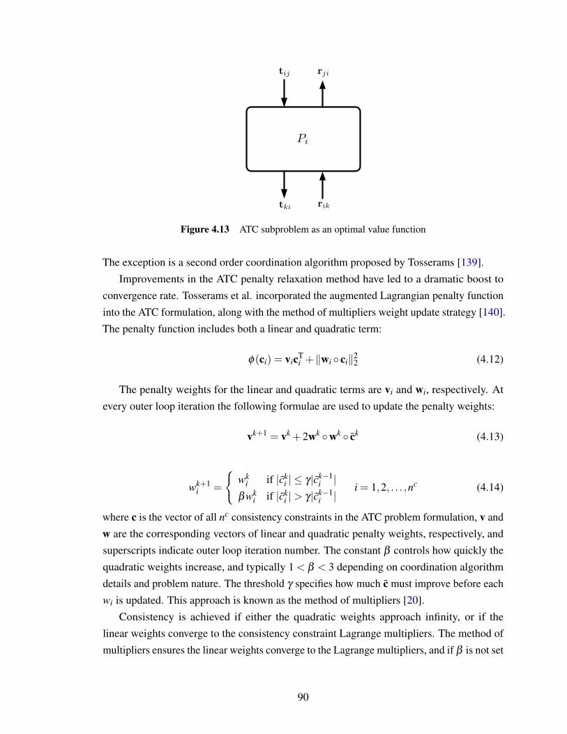
tij
tki rik
rji
Pi
Figure 4.13 ATC subproblem as an optimal value function
The exception is a second order coordination algorithm proposed by Tosserams [139].Improvements in the ATC penalty relaxation method have led to a dramatic boost to
convergence rate. Tosserams et al. incorporated the augmented Lagrangian penalty functioninto the ATC formulation, along with the method of multipliers weight update strategy [140].The penalty function includes both a linear and quadratic term:
φ(ci) = vicTi +‖wi ci‖2
2 (4.12)
The penalty weights for the linear and quadratic terms are vi and wi, respectively. Atevery outer loop iteration the following formulae are used to update the penalty weights:
vk+1 = vk +2wk wk ck (4.13)
wk+1i =
wk
i if |cki | ≤ γ|ck−1
i |βwk
i if |cki |> γ|ck−1
i |i = 1,2, . . . ,nc (4.14)
where c is the vector of all nc consistency constraints in the ATC problem formulation, v andw are the corresponding vectors of linear and quadratic penalty weights, respectively, andsuperscripts indicate outer loop iteration number. The constant β controls how quickly thequadratic weights increase, and typically 1 < β < 3 depending on coordination algorithmdetails and problem nature. The threshold γ specifies how much c must improve before eachwi is updated. This approach is known as the method of multipliers [20].
Consistency is achieved if either the quadratic weights approach infinity, or if thelinear weights converge to the consistency constraint Lagrange multipliers. The method ofmultipliers ensures the linear weights converge to the Lagrange multipliers, and if β is not set
90
too high ill conditioning is avoided. Convergence using a quadratic penalty alone frequentlyrequires hundreds or thousands of outer loop iterations. The augmented Lagrangian penaltyrelaxation method along with the method of multipliers converges much more quickly inpractice, sometimes in ten or fewer outer loop iterations [8]. In addition, the data requiredfor Eqs. 4.13 and 4.14 are more easily obtained than the derivatives required for Michalek’supdate method.
Several coordination algorithm variants are possible. Rather than solving the inner loopexactly at every outer loop iteration, we can terminate the inner loop fixed point iterationsolution when the system is consistent within a loose tolerance[140]. This approach isknown as the inexact method of multipliers (INMOM), whereas solving the inner loop towithin a very tight tolerance is called the exact method of multipliers (ENMOM). In anothercoordination alternative only a single pass of subproblem solutions is completed for everyouter loop iteration. This option is known as the alternating directions method of multipliers(ADMOM). A smaller value for β must be employed with ADMOM; otherwise quadraticweights will increase too quickly. ADMOM has exhibited the greatest efficiency of anyapproach, but does not fit within the assumptions required for the ATC convergence proof.In practice ADMOM works well for most problems.
A modification of the ADMOM approach exploits the hierarchical structure of ATC.Subproblems in each level are linked only to subproblems in adjacent levels. Subproblems inodd levels do not depend directly on outputs from other subproblems in odd levels. Therefore,all odd-level subproblems may be solved in parallel without having to use subproblemresponses from a previous iteration. The subproblems in even levels may then be executedsimultaneously. We alternate between solving all odd level subproblems in parallel andall even level subproblems in parallel. This odd-even coordination approach facilitates aneasily implemented parallel ATC solution process. Another possibility for a coordinatingsubproblems solved in parallel is Jacobi iteration [28]. Jacobi iteration is similar to fixed-point iteration, but when evaluating each subproblem we only use subproblem responsesfrom the previous iteration. This way all subproblems may be solved in parallel. Theadvantage of parallelism must be weighed against the slower convergence of Jacobi iteration[21].
4.3.3 Example: Aircraft Family Design
The aircraft family design problem, introduced in Section 3.3, is used here to illustrateimplementation of ATC. The objective of the aircraft family problem is to determine thedesign of two distinct aircraft used in a commercial airline fleet. Aircraft A is intended for
91
moderate range missions with up to 296 passengers. Aircraft B is intended for long rangemissions with up to 259 passengers. The main wing design is common between the aircraft,but all other components can be designed uniquely. The objective is to minimize a weightedaverage of pA and pB, the ticket prices for each aircraft, subject to performance constraints.
The problem is formulated as a bi-level ATC formulation with three subproblems. Thetop level problem P1 seeks to attain agreement between the lower-level subproblems withrespect to shared variables, while minimizing the system objective function f . The twolower-level problems, P2 and P3, seek to match targets set by P1, while meeting local designperformance constraints. P2 corresponds to the design of aircraft A, and P3 corresponds tothe design of aircraft B. This system has no feedback, simplifying the ATC formulation.Many other options for partitioning and formulation this problem exist, but are not addressedhere. In this partition each subproblem contains only one analysis function, so the sets ofexternal linking variables are equivalent to linking variables, and this is reflected in thenotation. For clarity in the ATC formulations, a superscript in parentheses indicates thesubproblem in which a value is computed. Problem P1 is formulated as:
minx(1)
s , p(1)A , p(1)
B
f(
p(1)A , p(1)
B
)+φ(c1) (4.15)
where: c1 =[x(1)
s x(1)s p(1)
A p(1)B
]−[x(2)
s x(3)s p(2)
A p(3)B
]The deviation vector c1 quantifies the difference between the targets set by P1 and the
achievable responses of P2 and P3. The responses are fixed parameters with respect to P1.Note that f is a function only of target cost metrics, since these are independent decisionvariables in P1. The penalty function φ(c1) helps guide the ATC process toward consistency.The linear and quadratic penalty weights, v1 and w1, are updated using the method ofmultipliers.
In this case the only analysis associated with P1 is the simple weighted average systemobjective function. When combined with the penalty function the P1 objective is a quadraticfunction, enabling direct solution without the use of an optimization algorithm. In addition,P1 has no design constraints, and therefore can be solved by finding x1 such that ∇x1 f1 = 0,where f1 = f +φ(c1). Problem P2 is formulated as:
92
minx(2)
s , x(2)`A
φ(c2)
subject to gA
(x(2)
s , x(2)`A
)≤ 0 (4.16)
where: c2 =[x(2)
s p(2)A
]−[x(1)
s p(1)A
]The formulation of Problem P3 is similar (one has simply to replace subscript or super-
script 2 with 3 and subscript A with B). The ADMOM approach was used to solve the ATCproblem.
The ATC subproblems P2 and P3 were solved using NOMADm [1], an implementationof mesh adaptive direct search [2, 14]. This algorithm effectively handled the non-smooth re-sponses of the PASS analysis software. The mesh tolerance used in determining NOMADmconvergence was 0.001, and subproblem optimizations typically required between 400 and600 function evaluations. ATC required between 8 and 18 NOMADm optimizations toobtain a solution, depending on the value chosen for β in the penalty updates.
The P1 subproblem objective function is quadratic, and required very little computationaleffort to solve. Two approaches were used to solve P1: solving for ∇x1 f1 = 0 (wheref1 = f + π(c)), and using a gradient-based algorithm to minimize f1. The former wasextremely efficient, but the latter proved more robust.
System consistency was quantified using the root mean square of the combined deviationvector
RMS(c) =
√1|c|
ccT ,
wherec = [c1, c2, c3] , |c|= cardinality of c.
The convergence of ATC was influenced strongly by the choice of β . Larger β valueshelp force the system into tighter consistency, but can result in a stiff system that requiresmore iterations to converge. The problem was solved using a range of different β values toillustrate this influence. Figure 4.14 illustrates how larger values of β require more outerloop iterations. It was also observed that larger β values led to slightly larger objectivefunction values, even when system consistency was approximately equal. This indicatesthat a stiff solution process can impede the identification of better designs.
93

1 2 3 4 5 6 7 8 90
0.01
0.02
0.03
0.04
0.05
0.06
0.07
0.08
0.09
0.1
ATC iteration number
RM
S(c)
ATC Convergence
β = 1.1β = 1.3
β = 1.5
β = 1.7
β = 1.9β = 2.1
Figure 4.14 Influence of β on RMS(c) (system consistency)
4.3.4 Augmented Lagrangian Coordination
The Augmented Lagrangian Coordination (ALC) formulation, also known as AugmentedLagrangian Decomposition, utilizes principles from ATC for the solution of a more generalclass of system design problems. The problem structure in ALC is not limited to hierarchical;any type of links between subproblems can be managed. Convergence properties are drawnfrom established nonlinear programming theory. ALC provides tremendous flexibility inproblem linking structure, making it an ideal platform for studying the linking structureaspect of coordination decisions. ALC can handle linking functions in addition to linkingvariables. Linking functions depend on most or all design variables. This situation isuncommon in simulation-based design optimization, so accommodation of linking functionswill not be included in the formulations here. ALC uses a double-loop coordination algorithmwith augmented Lagrangian penalty relaxation, similar to ATC. The coordination algorithmvariants described above, such as INMOM, ADMOM, and Jacobi iteration, all apply toALC.
As with other distributed optimization formulations, local copies of linking variablesmust be used in ALC subproblems. These copies are allowed to vary independently,enabling independent subproblem solution, but are guided toward consistency using penaltyfunctions. Internal shared design variables for subproblem i (xsi) do not require multiplecopies since they are determined by the same optimization algorithm, and therefore requireno consistency constraints. The internal coupling variables for subproblem i are yi, and thecorresponding set of analysis functions is ai(xi, yi, yi), where yi are the external coupling
94
variables input to subproblem i and xi are the design variables for subproblem i. Thesevalues must be consistent. An MDF-type approach could be used here to satisfy internalconsistency requirements with an analysis algorithm such as fixed point iteration. Analternative approach is to enforce internal consistency using auxiliary equality constraints:
ci(xi, yi, yi) = yi− ai(xi, yi, yi) = 0 (4.17)
This auxiliary equality constraint approach draws from the principles underlying theIDF formulation. Section 4.2 discussed how computational performance and robustness canbe enhanced through using equality constraints instead of FPI to satisfy consistency require-ments. The auxiliary constraints in Eq. 4.17 will be used in subsequent ALC formulations.
Definition of external linking variable consistency constraints is somewhat more involved.The copies of design variables shared between subproblems i and j, local to subproblem i,are xi j
s . The coupling variables passed from subproblem j to i are yi j, and the correspondinganalysis functions are ai j(x j, y j, y j). The external linking variables between subproblems i
and j are zi j = [xi js , yi j]. The external consistency constraints between subproblems i and j
are:
ci j(xi, x j, yi, y j, yi, y j) =[yi j− ai j(x j, y j, y j), y ji− a ji(xi, yi, yi), xi j
s − x jis]
(4.18)
Note that the components of xi js are part of the vector xi, and yi j is part of the vector
yi. Certain variables that are input to the constraint function ci j are held fixed duringsubproblem solution, as indicated by the input arguments of the consistency constraint inthe ALC subproblem formulation presented shortly.
The definitions above specify a very large number of consistency constraints for externalshared variables. Only a subset of these constraints is required to ensure consistency. Thenumber of possible ways to allocate consistency constraints is tremendous, and is a taskbeyond intuition for all but the smallest system design problems. Guidelines have beenproposed for constructing bi-level or hierarchical ALC implementations [141, 142]. Theserecommendations are helpful, but do not capitalize on the potential benefit that couldbe realized through tailoring problem structure to meet the needs of a system. Chapter7 develops the theory towards a rigorous, automated method for allocating consistencyconstraints.
After a set of consistency constraints is selected and allocated amongst the subproblems,an augmented Lagrangian penalty function is defined for the selected constraints on externallinking variables:
φi j(ci j) = vi jcTi j +‖wi j ci j‖2
2 (4.19)
95
where vi j and wi j are vectors of penalty weights on the linear and quadratic terms, respec-tively, and indicates the Hadamard product. Penalty weights are fixed for one or moreinner loop executions, and are updated using the method of multipliers.
The set of indices for subproblems with external linking variables common to subproblemi is Ni. The design inequality and equality constraints computed by analysis functions insubproblem i are gi and hi, respectively. The set of decision variables for subproblem i
includes xi, yi, and yi. The formulation of the optimization problem for subproblem i is:
minxi,yi,yi
fi(xi, yi, yi)+ ∑j∈Ni| j>i
φi j(ci j(xi, yi j, yi))
+ ∑j∈Ni| j<i
φ ji(c ji(xi, yi j, yi)) (4.20)
subject to gi(xi, yi, yi)≤ 0
hi(xi, yi, yi) = 0,
ci(xi, yi, yi) = yi− a(xi, yi, yi) = 0
This formulation makes a distinction between shared and coupling variables, in con-trast to the original ALC formulations [141, 142]. Neglecting this distinction requires anadditional equality constraint for each analysis function that computes a coupling variable.Accounting for the distinction requires only one quantity to be passed for every couplingvariable between subproblems, instead of two, and permits exploitation of coupling variabledirectionality when structuring an ALC implementation.
4.3.5 Example: Air Flow Sensor Design
The air flow sensor design from Section 3.1 is used here to illustrate ALC formulation andimplementation. An ALC subproblem is formulated for the aerodynamic and structuralaspects of the design problem. The structural subproblem is P1 and the aerodynamicsubproblem is P2. The formulation for the structural subproblem is:
min`(1),F(1)
(θ (1)− θ)2 +v12c12 +‖w12 c12‖22
subject to F(1)−Fmax ≤ 0 (4.21)
where c12(`(1),F(1)) = [θ (1)−θ(2),F(1)−F(2), `(1)− `(2)]
Superscripts indicate the subproblem quantities are computed in. The constraint c12
96
was chosen arbitrarily for this implementation rather than c21. The stator deflection θ (1) iscomputed using Eq. 3.2. The value of θ (2) is a fixed parameter in the subproblem 1, andis determined by subproblem 2. θ and F are coupling variables, and ` is a shared designvariable. Although the drag force analysis is part of subproblem 2, problem convergencewas improved by locating it in subproblem 1. The formulation for subproblem 2 is:
min`(2),w(2),θ (2)
v12c12 +‖w12 c12‖22
subject to `(2)w(2)−A = 0 (4.22)
where c12(`(2),w(2),θ (2)) = [θ (1)−θ(2),F(1)−F(2), `(1)− `(2)]
The aerodynamic subproblem has no local design objective function, so the optimizationobjective is the penalty function on c21 only. Note that the constraint c21 is defined identicallyin subproblem 2 except for the input arguments. Here θ (2) and `(2) are independent variables,while θ (1), F(1), and `(1) are fixed parameters determined by subproblem 1. The drag forceF(2) is computed using Eq. 3.3.
The ALC solution was implemented using the ENMOM approach and the result matchedthe optimal design determined by monotonicity analysis. The outer loop parameters usedwere β = 2.2 and γ = 0.40. Ten outer loop iterations were required to satisfy the convergencecriterion of ‖c‖ ≤ 1.0 ·10−4. Inner loop convergence required that the normalized sum ofsubproblem objective functions was less than 1.0 ·10−4. Table 4.1 summarizes the ALCsolution process for this problem, where i is the outer loop iteration number, j is the innerloop iteration number, and n f is the number of function evaluations required for each outerloop iteration. The number of inner loop iterations is larger at the beginning of the process,but decreases as the solution is approached. The number of function evaluations indicatesthat the difficulty of the subproblems gradually increased during most of the process, butthen dropped off near the end.
Karsemakers studied the air flow sensor design problem at length and showed thatmodifying problem structure or the coordination algorithm had significant influence overcomputational expense [76]. In some cases the computational benefit exceeded one orderof magnitude. Chapters 5 through 7 will develop a formal approach for choosing systempartitions and coordination algorithms for ALC and related formulations.
97

4.4 Concluding Comments
This chapter reviewed several important formulations for decomposition-based designoptimization, which fall under two categories: single-level and multi-level. Single-levelformulations may employ a distributed analysis approach, but use a single optimizationalgorithm for the entire system. Single-level formulations meet the requirements of systemconsistency and optimality, and can help ease system analysis difficulties, but may beinappropriate for problems with a very large number of design variables. Multi-levelformulations address this problem by using a distributed optimization approach; a separateoptimization problem is defined for each subproblem, reducing the total number of designvariables that must be managed by any single optimization algorithm. Several exampleswere used to explain the formulations covered in this chapter. Parametric studies on couplingstrength and algorithm parameters were performed, providing important insights into theformulations reviewed. The understanding of system optimization formulations developedin this chapter is a foundation for the quantitative approach to partitioning and coordinationdecisions presented in the following chapter.
Table 4.1 ALC solution progress for the air-flow sensor problemi j n f1 3 1742 6 1913 3 1294 5 6585 4 4426 3 3547 3 2978 2 1689 2 9010 2 88
98
Chapter 5
Optimal Partitioning and Coordination: TheoreticalFramework
Solving a system design optimization problem using decomposition-based design optimiza-tion requires that a system partition and coordination strategy be defined a priori. Partitioningand coordination (P/C) decisions can have a profound effect on computational expense of thesolution process. P/C decisions should minimize the complexity of the resulting distributedoptimization problem. The solution difficulty for a system design problem given a particularset of P/C decisions is difficult to estimate without actually solving the problem, but isrequired for P/C decision optimization to be beneficial. Complexity is approximated hereby the coordination problem size (CS) and the maximum subproblem size (SSmax). Thesemetrics can be estimated using the reduced adjacency matrix for a system and the proposedsystem partition and coordination strategy.
The primary objective in this chapter is to demonstrate that P/C decisions are coupled;i.e., a system partition will influence what coordination strategy should be chosen, and viceversa. Section 1.1 described how an independent or sequential approach to design can lead tosuboptimal solutions if coupling is present. This applies to the P/C optimal decision problemas well. Independent, sequential, and simultaneous approaches are formulated for solving theP/C problem, and it is shown that for three example systems only the simultaneous approachis successful. This is evidence of coupling between partitioning and coordination decisions.Coordination strategy decisions are limited to subproblem sequence in this chapter. Thissimplifies the analysis here, but provides sufficient modeling fidelity to identify couplingand study tradeoffs. Tradeoff information may be used to assess the appropriateness ofdecomposition-based design optimization for a particular system.
5.1 P/C Problem Formulation
The objective in the optimal P/C decision problem is to find a system partition and subprob-lem sequence that minimizes overall computational expense of the system design solution
99
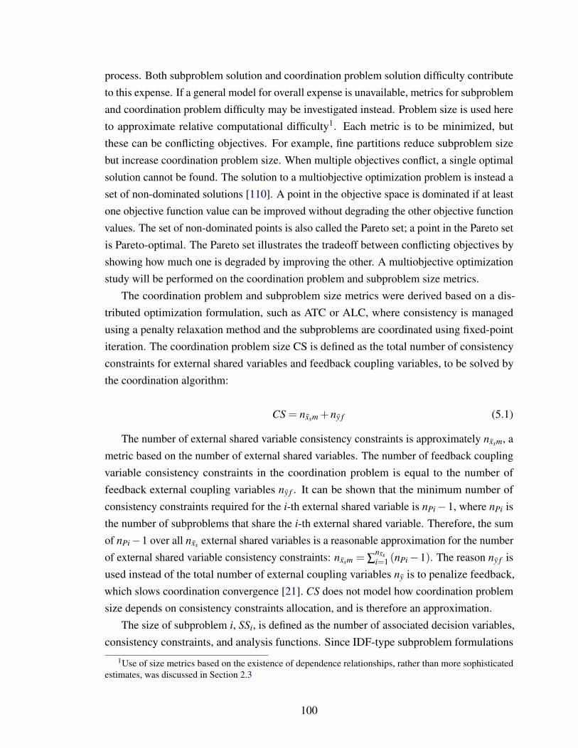
process. Both subproblem solution and coordination problem solution difficulty contributeto this expense. If a general model for overall expense is unavailable, metrics for subproblemand coordination problem difficulty may be investigated instead. Problem size is used hereto approximate relative computational difficulty1. Each metric is to be minimized, butthese can be conflicting objectives. For example, fine partitions reduce subproblem sizebut increase coordination problem size. When multiple objectives conflict, a single optimalsolution cannot be found. The solution to a multiobjective optimization problem is instead aset of non-dominated solutions [110]. A point in the objective space is dominated if at leastone objective function value can be improved without degrading the other objective functionvalues. The set of non-dominated points is also called the Pareto set; a point in the Pareto setis Pareto-optimal. The Pareto set illustrates the tradeoff between conflicting objectives byshowing how much one is degraded by improving the other. A multiobjective optimizationstudy will be performed on the coordination problem and subproblem size metrics.
The coordination problem and subproblem size metrics were derived based on a dis-tributed optimization formulation, such as ATC or ALC, where consistency is managedusing a penalty relaxation method and the subproblems are coordinated using fixed-pointiteration. The coordination problem size CS is defined as the total number of consistencyconstraints for external shared variables and feedback coupling variables, to be solved bythe coordination algorithm:
CS = nxsm +ny f (5.1)
The number of external shared variable consistency constraints is approximately nxsm, ametric based on the number of external shared variables. The number of feedback couplingvariable consistency constraints in the coordination problem is equal to the number offeedback external coupling variables ny f . It can be shown that the minimum number ofconsistency constraints required for the i-th external shared variable is nPi−1, where nPi isthe number of subproblems that share the i-th external shared variable. Therefore, the sumof nPi−1 over all nxs external shared variables is a reasonable approximation for the numberof external shared variable consistency constraints: nxsm = ∑
nxsi=1 (nPi−1). The reason ny f is
used instead of the total number of external coupling variables ny is to penalize feedback,which slows coordination convergence [21]. CS does not model how coordination problemsize depends on consistency constraints allocation, and is therefore an approximation.
The size of subproblem i, SSi, is defined as the number of associated decision variables,consistency constraints, and analysis functions. Since IDF-type subproblem formulations
1Use of size metrics based on the existence of dependence relationships, rather than more sophisticatedestimates, was discussed in Section 2.3
100
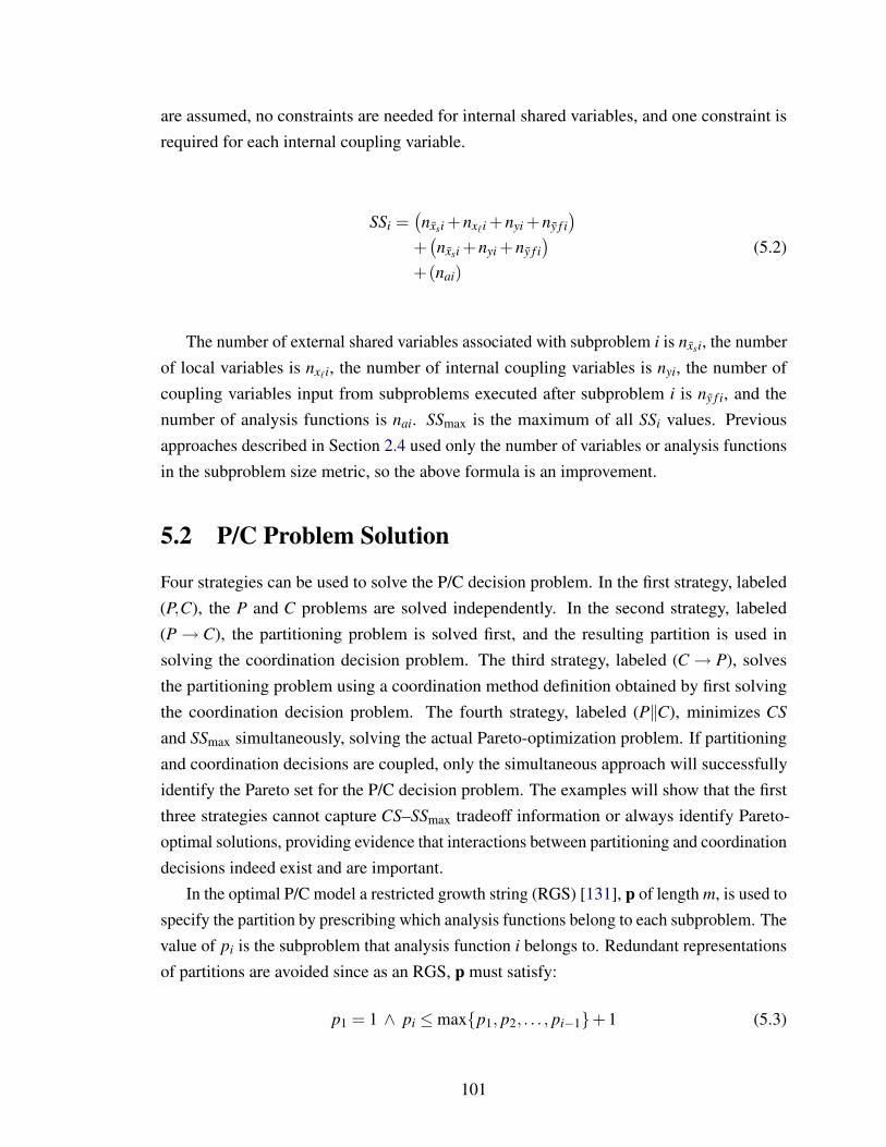
are assumed, no constraints are needed for internal shared variables, and one constraint isrequired for each internal coupling variable.
SSi =(nxsi +nx`i +nyi +ny f i
)+(nxsi +nyi +ny f i
)(5.2)
+(nai)
The number of external shared variables associated with subproblem i is nxsi, the numberof local variables is nx`i, the number of internal coupling variables is nyi, the number ofcoupling variables input from subproblems executed after subproblem i is ny f i, and thenumber of analysis functions is nai. SSmax is the maximum of all SSi values. Previousapproaches described in Section 2.4 used only the number of variables or analysis functionsin the subproblem size metric, so the above formula is an improvement.
5.2 P/C Problem Solution
Four strategies can be used to solve the P/C decision problem. In the first strategy, labeled(P,C), the P and C problems are solved independently. In the second strategy, labeled(P→ C), the partitioning problem is solved first, and the resulting partition is used insolving the coordination decision problem. The third strategy, labeled (C→ P), solvesthe partitioning problem using a coordination method definition obtained by first solvingthe coordination decision problem. The fourth strategy, labeled (P‖C), minimizes CS
and SSmax simultaneously, solving the actual Pareto-optimization problem. If partitioningand coordination decisions are coupled, only the simultaneous approach will successfullyidentify the Pareto set for the P/C decision problem. The examples will show that the firstthree strategies cannot capture CS–SSmax tradeoff information or always identify Pareto-optimal solutions, providing evidence that interactions between partitioning and coordinationdecisions indeed exist and are important.
In the optimal P/C model a restricted growth string (RGS) [131], p of length m, is used tospecify the partition by prescribing which analysis functions belong to each subproblem. Thevalue of pi is the subproblem that analysis function i belongs to. Redundant representationsof partitions are avoided since as an RGS, p must satisfy:
p1 = 1 ∧ pi ≤maxp1, p2, . . . , pi−1+1 (5.3)
101
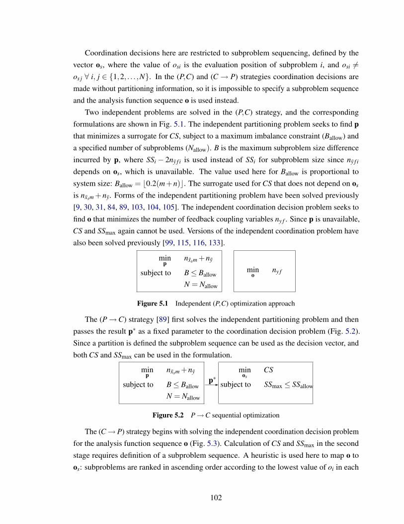
Coordination decisions here are restricted to subproblem sequencing, defined by thevector os, where the value of osi is the evaluation position of subproblem i, and osi 6=os j ∀ i, j ∈ 1,2, . . . ,N. In the (P,C) and (C→ P) strategies coordination decisions aremade without partitioning information, so it is impossible to specify a subproblem sequenceand the analysis function sequence o is used instead.
Two independent problems are solved in the (P,C) strategy, and the correspondingformulations are shown in Fig. 5.1. The independent partitioning problem seeks to find pthat minimizes a surrogate for CS, subject to a maximum imbalance constraint (Ballow) anda specified number of subproblems (Nallow). B is the maximum subproblem size differenceincurred by p, where SSi− 2ny f i is used instead of SSi for subproblem size since ny f i
depends on os, which is unavailable. The value used here for Ballow is proportional tosystem size: Ballow = b0.2(m+n)c. The surrogate used for CS that does not depend on os
is nxsm +ny. Forms of the independent partitioning problem have been solved previously[9, 30, 31, 84, 89, 103, 104, 105]. The independent coordination decision problem seeks tofind o that minimizes the number of feedback coupling variables ny f . Since p is unavailable,CS and SSmax again cannot be used. Versions of the independent coordination problem havealso been solved previously [99, 115, 116, 133].
minp
nxsm +ny
subject to B≤ Ballow
N = Nallow
mino
ny f
Figure 5.1 Independent (P,C) optimization approach
The (P→C) strategy [89] first solves the independent partitioning problem and thenpasses the result p∗ as a fixed parameter to the coordination decision problem (Fig. 5.2).Since a partition is defined the subproblem sequence can be used as the decision vector, andboth CS and SSmax can be used in the formulation.
minp
nxsm +ny
subject to B≤ Ballow
N = Nallow
-p∗
minos
CS
subject to SSmax ≤ SSallow
Figure 5.2 P→C sequential optimization
The (C→ P) strategy begins with solving the independent coordination decision problemfor the analysis function sequence o (Fig. 5.3). Calculation of CS and SSmax in the secondstage requires definition of a subproblem sequence. A heuristic is used here to map o toos: subproblems are ranked in ascending order according to the lowest value of oi in each
102

subproblem to define the subproblem sequence.
mino
ny f -o∗
minp
CS
subject to SSmax ≤ SSallow
Figure 5.3 C→ P sequential optimization
The (P‖C) strategy seeks optimal values for p and os simultaneously. The multiobjectiveproblem to be solved is:
minp,os
CS,SSmax (5.4)
The set of Pareto-optimal solutions can be obtained by solving the single-objectiveoptimization problem shown in Fig. 5.4 and varying SSmax as a parameter.
minp,os
CS
subject to SSmax ≤ SSallow
Figure 5.4 Simultaneous (P‖C) optimization
5.3 Examples
The four strategies were applied to two randomly generated reduced adjacency matrices todemonstrate the tradeoff between CS and SSmax and the interaction between partitioning andcoordination decisions. The optimal P/C decision problems were all solved using exhaustiveenumeration, and the appropriate constraints were varied in an effort to generate Pareto sets.
The first example has five analysis functions and seven design variables; its reducedadjacency matrix is:
A1 =
0 1 1 1 0 1 0 1 1 1 0 10 0 1 1 1 0 1 1 0 1 1 11 0 0 1 1 1 1 1 1 1 1 11 1 1 0 0 1 1 1 1 1 1 11 1 0 1 0 0 1 1 1 0 0 1
Figure 5.5 depicts the histogram of all possible CS and SSmax values for an exhaustive
enumeration of all possible p and os combinations. The CS distribution is biased towardlarger values, while the SSmax is biased toward smaller values. This is expected since thenumber of possible sequences and partitions increase with N, and CS decreases with N whileSSmax increases with N. Figure 5.6 plots all P/C instances for A1 in the CS/SSmax space. In
103
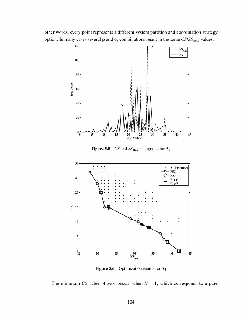
other words, every point represents a different system partition and coordination strategyoption. In many cases several p and os combinations result in the same CS/SSmax values.
0 5 10 15 20 25 30 35 40 450
20
40
60
80
100
120
Size Metric
freq
uenc
y
SSmax
CS
Figure 5.5 CS and SSmax histograms for A1
15 20 25 30 35 40 450
5
10
15
20
25
30
SSmax
CS
All InstancesP||CP,CP−>CC−>P
Figure 5.6 Optimization results for A1
The minimum CS value of zero occurs when N = 1, which corresponds to a pure
104
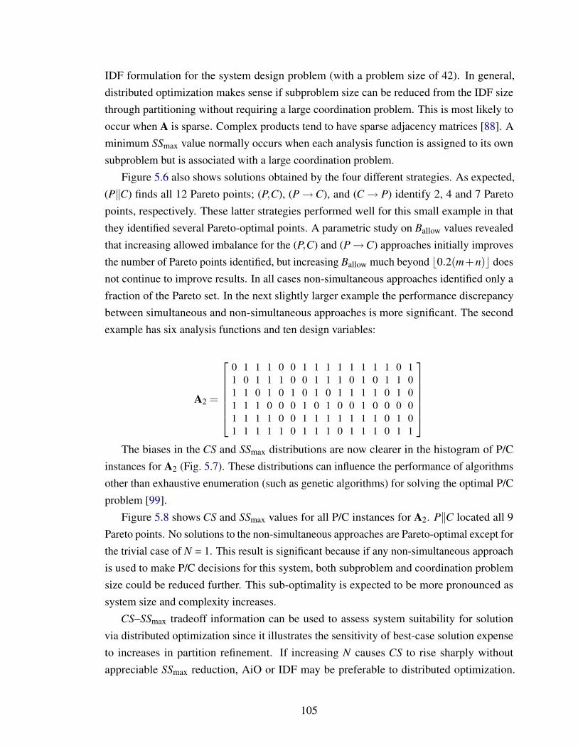
IDF formulation for the system design problem (with a problem size of 42). In general,distributed optimization makes sense if subproblem size can be reduced from the IDF sizethrough partitioning without requiring a large coordination problem. This is most likely tooccur when A is sparse. Complex products tend to have sparse adjacency matrices [88]. Aminimum SSmax value normally occurs when each analysis function is assigned to its ownsubproblem but is associated with a large coordination problem.
Figure 5.6 also shows solutions obtained by the four different strategies. As expected,(P‖C) finds all 12 Pareto points; (P,C), (P→C), and (C→ P) identify 2, 4 and 7 Paretopoints, respectively. These latter strategies performed well for this small example in thatthey identified several Pareto-optimal points. A parametric study on Ballow values revealedthat increasing allowed imbalance for the (P,C) and (P→C) approaches initially improvesthe number of Pareto points identified, but increasing Ballow much beyond b0.2(m+n)c doesnot continue to improve results. In all cases non-simultaneous approaches identified only afraction of the Pareto set. In the next slightly larger example the performance discrepancybetween simultaneous and non-simultaneous approaches is more significant. The secondexample has six analysis functions and ten design variables:
A2 =
0 1 1 1 0 0 1 1 1 1 1 1 1 1 0 11 0 1 1 1 0 0 1 1 1 0 1 0 1 1 01 1 0 1 0 1 0 1 0 1 1 1 1 0 1 01 1 1 0 0 0 1 0 1 0 0 1 0 0 0 01 1 1 1 0 0 1 1 1 1 1 1 1 0 1 01 1 1 1 1 0 1 1 1 0 1 1 1 0 1 1
The biases in the CS and SSmax distributions are now clearer in the histogram of P/C
instances for A2 (Fig. 5.7). These distributions can influence the performance of algorithmsother than exhaustive enumeration (such as genetic algorithms) for solving the optimal P/Cproblem [99].
Figure 5.8 shows CS and SSmax values for all P/C instances for A2. P‖C located all 9Pareto points. No solutions to the non-simultaneous approaches are Pareto-optimal except forthe trivial case of N = 1. This result is significant because if any non-simultaneous approachis used to make P/C decisions for this system, both subproblem and coordination problemsize could be reduced further. This sub-optimality is expected to be more pronounced assystem size and complexity increases.
CS–SSmax tradeoff information can be used to assess system suitability for solutionvia distributed optimization since it illustrates the sensitivity of best-case solution expenseto increases in partition refinement. If increasing N causes CS to rise sharply withoutappreciable SSmax reduction, AiO or IDF may be preferable to distributed optimization.
105
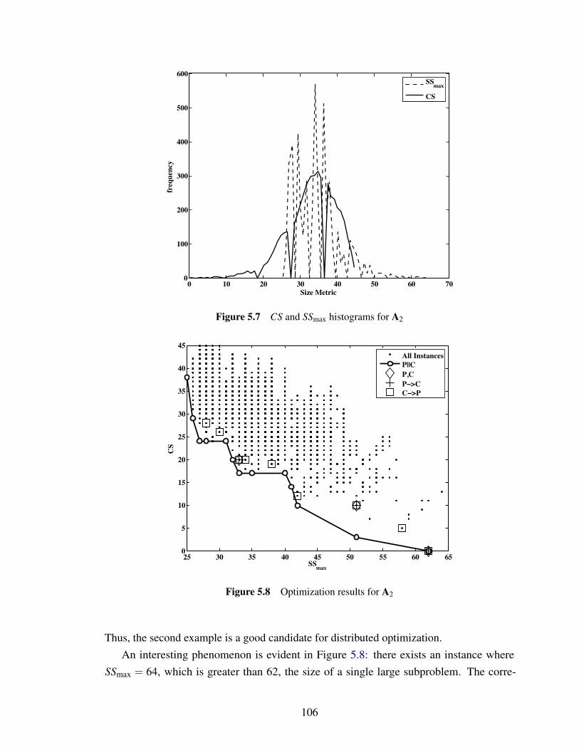
0 10 20 30 40 50 60 700
100
200
300
400
500
600
Size Metric
freq
uenc
y
SSmax
CS
Figure 5.7 CS and SSmax histograms for A2
25 30 35 40 45 50 55 60 650
5
10
15
20
25
30
35
40
45
SSmax
CS
All InstancesP||CP,CP−>CC−>P
Figure 5.8 Optimization results for A2
Thus, the second example is a good candidate for distributed optimization.An interesting phenomenon is evident in Figure 5.8: there exists an instance where
SSmax = 64, which is greater than 62, the size of a single large subproblem. The corre-
106
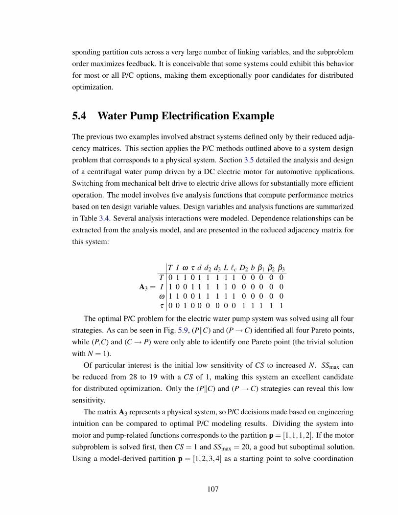
sponding partition cuts across a very large number of linking variables, and the subproblemorder maximizes feedback. It is conceivable that some systems could exhibit this behaviorfor most or all P/C options, making them exceptionally poor candidates for distributedoptimization.
5.4 Water Pump Electrification Example
The previous two examples involved abstract systems defined only by their reduced adja-cency matrices. This section applies the P/C methods outlined above to a system designproblem that corresponds to a physical system. Section 3.5 detailed the analysis and designof a centrifugal water pump driven by a DC electric motor for automotive applications.Switching from mechanical belt drive to electric drive allows for substantially more efficientoperation. The model involves five analysis functions that compute performance metricsbased on ten design variable values. Design variables and analysis functions are summarizedin Table 3.4. Several analysis interactions were modeled. Dependence relationships can beextracted from the analysis model, and are presented in the reduced adjacency matrix forthis system:
A3 =
T I ω τ d d2 d3 L `c D2 b β1 β2 β3T 0 1 1 0 1 1 1 1 1 0 0 0 0 0I 1 0 0 1 1 1 1 1 0 0 0 0 0 0ω 1 1 0 0 1 1 1 1 1 0 0 0 0 0τ 0 0 1 0 0 0 0 0 0 1 1 1 1 1
The optimal P/C problem for the electric water pump system was solved using all fourstrategies. As can be seen in Fig. 5.9, (P‖C) and (P→C) identified all four Pareto points,while (P,C) and (C→ P) were only able to identify one Pareto point (the trivial solutionwith N = 1).
Of particular interest is the initial low sensitivity of CS to increased N. SSmax canbe reduced from 28 to 19 with a CS of 1, making this system an excellent candidatefor distributed optimization. Only the (P‖C) and (P→ C) strategies can reveal this lowsensitivity.
The matrix A3 represents a physical system, so P/C decisions made based on engineeringintuition can be compared to optimal P/C modeling results. Dividing the system intomotor and pump-related functions corresponds to the partition p = [1,1,1,2]. If the motorsubproblem is solved first, then CS = 1 and SSmax = 20, a good but suboptimal solution.Using a model-derived partition p = [1,2,3,4] as a starting point to solve coordination
107
12 14 16 18 20 22 24 26 280
2
4
6
8
10
12
14
SSmax
CS
All InstancesP||CP,CP−>CC−>P
Figure 5.9 Optimal P/C results for pump problem
problem defined in Fig. 5.2 for the optimal sequence, the solution o∗s = [4,3,2,1] yieldsCS = 12 and SSmax = 13, which is a Pareto point. In this simple example, intuitive andsemi-intuitive approaches are rather effective, but cannot quantify the tradeoff betweenCS and SSmax. Much larger systems are likely to realize greater benefits from the (P‖C)strategy, but algorithms more sophisticated than exhaustive enumeration are required in suchimplementations. One approach to solve the P/C problem for larger systems is presented inthe following chapter.
5.5 Concluding Comments
A formal approach for simultaneous partitioning and coordination decision-making waspresented in this chapter. The approach quantifies P–C tradeoffs by computing Paretooptima for minimum subproblem size and coordination problem size. Studying thesetradeoffs helps determine whether a system design problem is an appropriate candidatefor decomposition-based design optimization. The problem-size metrics proposed herecaptured P/C interactions in the examples successfully. Other metrics that approximatethe tradeoff between coordination and subproblem expense can be used instead if desired.Simultaneous P/C optimization can lead to superior decomposition solutions. Comparison tonon-simultaneous strategies confirmed the existence of P/C decision interaction, and demon-
108

strated the value of a simultaneous approach. Exhaustive enumeration was used to generateresults for small examples, and a simplified coordination decision model incorporated onlysubproblem sequencing. Following chapters demonstrate how to solve the P/C problem forlarger systems, and how to incorporate linking structure into coordination decisions.
109
Chapter 6
Extension to Larger Systems
The previous chapter demonstrated that partitioning and coordination decisions are coupledfor several example systems, and illustrated tradeoffs present in these decisions. A multiob-jective optimization problem was defined, and exact solutions were obtained in each caseusing exhaustive enumeration. The discrete decision space of Eq. (5.4) is vast; the numberof possible partitioning and coordination instances increases exponentially with the numberof analysis functions. The P‖C problem for systems with more than seven analysis functionscannot be solved in a practical amount of time using exhaustive enumeration. The parti-tioning and sequencing problems are themselves NP-complete [129] and NP-hard [124],respectively, making the combined partitioning and coordination problem an especiallydifficult problem.
Evolutionary algorithms (EAs) have proven to be an effective tool for approximatelysolving difficult combinatorial optimization problems. This chapter reviews the conceptsof EAs and presents the results of applying an EA to a system too large for exhaustiveenumeration. An EA developed for solving the P‖C problem is applied to the examplesystems of Chapter 5. Comparison of EA results to exact solutions provides validation ofthe algorithm. The truss design formulation from Section 3.4 is used to generate a systemwith eight analysis functions. The EA is then used to obtain an approximate Pareto set forthis system. The results indicate that the EA is an effective solution technique for systemsof practical size.
6.1 Evolutionary Algorithms
Evolutionary algorithms are a class of algorithms for solving a variety of difficult problemsusing a process patterned after natural evolution. In biological populations, individuals mostwell-suited for their environment tend to survive to reproduce and generate offspring. Thisnatural selection process moves to increase the overall ‘fitness’ of a population over time.Two primary operations are exercised: variation and selection. Variation takes place when
110
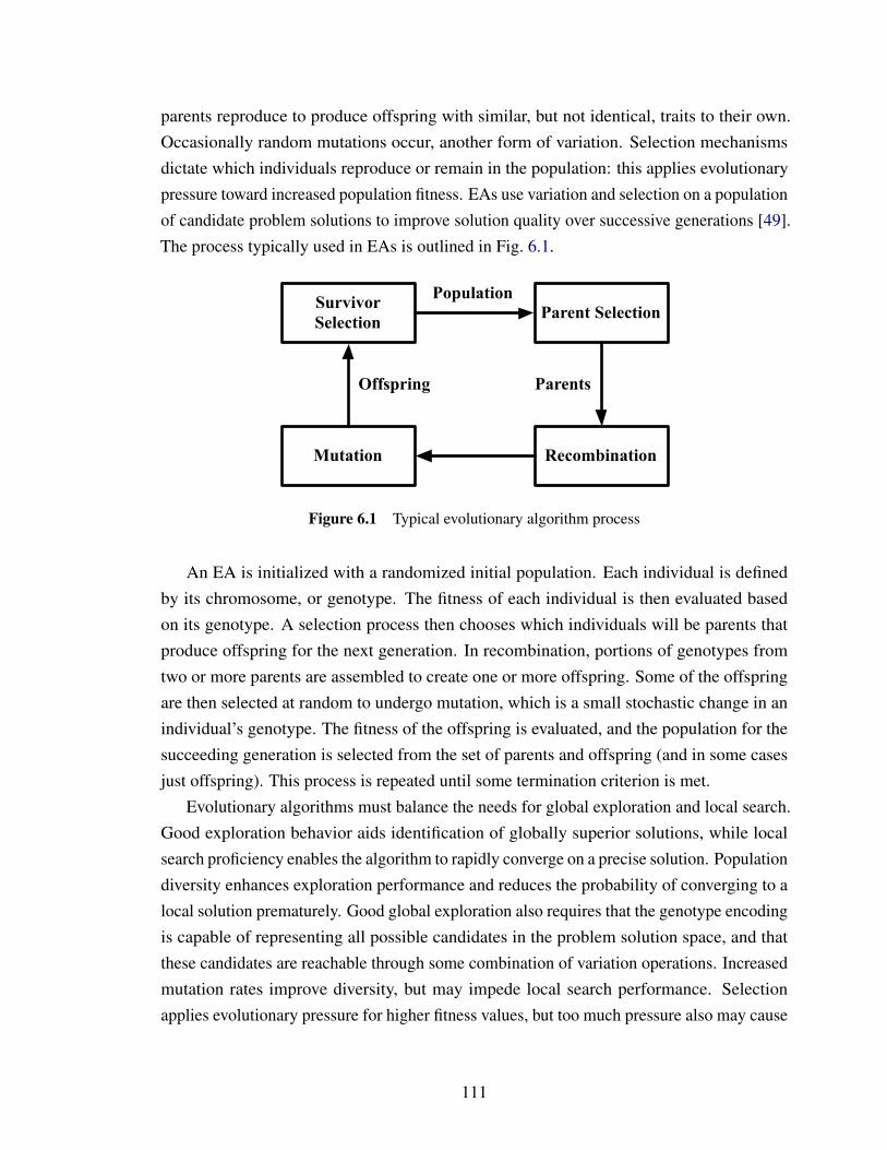
parents reproduce to produce offspring with similar, but not identical, traits to their own.Occasionally random mutations occur, another form of variation. Selection mechanismsdictate which individuals reproduce or remain in the population: this applies evolutionarypressure toward increased population fitness. EAs use variation and selection on a populationof candidate problem solutions to improve solution quality over successive generations [49].The process typically used in EAs is outlined in Fig. 6.1.
Parent Selection
RecombinationMutation
Survivor Selection
Population
ParentsOffspring
Figure 6.1 Typical evolutionary algorithm process
An EA is initialized with a randomized initial population. Each individual is definedby its chromosome, or genotype. The fitness of each individual is then evaluated basedon its genotype. A selection process then chooses which individuals will be parents thatproduce offspring for the next generation. In recombination, portions of genotypes fromtwo or more parents are assembled to create one or more offspring. Some of the offspringare then selected at random to undergo mutation, which is a small stochastic change in anindividual’s genotype. The fitness of the offspring is evaluated, and the population for thesucceeding generation is selected from the set of parents and offspring (and in some casesjust offspring). This process is repeated until some termination criterion is met.
Evolutionary algorithms must balance the needs for global exploration and local search.Good exploration behavior aids identification of globally superior solutions, while localsearch proficiency enables the algorithm to rapidly converge on a precise solution. Populationdiversity enhances exploration performance and reduces the probability of converging to alocal solution prematurely. Good global exploration also requires that the genotype encodingis capable of representing all possible candidates in the problem solution space, and thatthese candidates are reachable through some combination of variation operations. Increasedmutation rates improve diversity, but may impede local search performance. Selectionapplies evolutionary pressure for higher fitness values, but too much pressure also may cause
111

premature convergence.Genotype representation is an important aspect of implementing an EA for a specific
problem. Examples of established genotype representation types include binary or real-valued strings. In EAs variation operators are applied to genotype representations ofindividuals. The representation of an individual in the original problem formulation iscalled its phenotype. Sometimes the phenotype representation is congruent with a standardgenotype representation and can be used directly with modification to the EA. When thisis not the case one of two approaches may be taken. First, the phenotype representationmay be used directly if variation operators compatible with the representation are developed.A large body of work exists regarding specialized variation operators for solving specifictypes of problems [49]. Second, an appropriate genotype space must be defined along witha surjective mapping onto the phenotype space. Rothlauf developed a theory-based method-ology for defining effective genotype representations [118]. An ideal representation shouldnot increase problem difficulty, should enable variation operators to work properly, andshould result in a process that is robust to solution location. To meet these requirements it isimportant that a representation have good locality and little bias toward particular genotypes.Good locality ensures that small changes in the genotype space result in small changesin the phenotype space. Poor locality impacts both global exploration and local searchperformance. A representation biased toward solution candidates with certain propertiesmay result in failure to identify globally superior solutions.
An important feature of EAs is effectiveness for multiobjective problems (MOPs). Thesolution to an MOP is a set of non-dominated points (i.e., the Pareto set), rather than asingle point solution. EAs are population-based, and are naturally equipped to seek aftera set solution. Goldberg proposed a fitness function based on the dominance of candidatesolutions, rather than the multiple objective values [65]. This approach enables an EA toidentify an approximate Pareto set with a single execution of the algorithm. TraditionalMOP solution approaches require that the optimization algorithm be solved multiple timeswith different objective function or constraint parameters.
Several variants of EAs have been developed to address specific problem types [49].Each variant has a unique approach for implementing the EA process illustrated in Fig. 6.1.Genetic algorithms (GAs) were introduced by Holland [73], and are typically used forcombinatorial optimization problems. Recombination is the primary variation operator,while mutation plays a lesser role. Genotypes are typically represented using binary orinteger strings. Fogel, Owens, and Walsh developed evolutionary programming (EP) [54],commonly used for continuous optimization. Real-valued strings are normally used as thegenotype representation, and mutation is the sole variation operator. Evolutionary strategies
112
(ES) were proposed by Rechenberg [113], and are also used for continuous optimizationwith real-valued genotype representations. Mutation is the primary variation operator, whilerecombination is secondary. A distinguishing feature of ES is self-adaptation. Most EAshave numerous algorithm parameters that must be tuned for efficient performance, and hasbeen touted as a significant weakness concerning EA practicality. Self-adaptation includesalgorithm parameters in the genotype so that as the algorithm progresses, it determinesthe ideal parameters required to solve the problem at hand effectively. Later on Kozaintroduced genetic programming (GP) as a technique specifically for automated computercode generation [83]. Some programming languages, such as Lisp [122], are naturallyexpressed in a tree1 structure; GP utilizes a tree genotype representation, and specializedrecombination and mutation techniques that operate directly on trees.
Eiben explained that EAs are effective at solving difficult problems with acceptableresults in a reasonable amount of time [49]. While EAs are frequently applied to optimizationproblems, they are not strictly optimization algorithms [40]. EAs are not based on anytype of optimality conditions, and therefore cannot guarantee optimality of results. Manyoptimization problems cannot be solved exactly in a practical amount of time, but EAs offera way to obtain approximately optimal results in a satisfactory period of time.
While EAs have proven to be effective at solving difficult problems [48], no singlealgorithm within this class is ideal for solving all problems. Wolpert and Macready setforth the ‘no free lunch’ theorem, which asserts that if we average the performance ofnonrevisiting2 black box algorithms over all possible problems, all algorithms performequally well [146]. In other words, if a particular algorithm is well-suited for one type ofproblem, then it will not be effective at solving a distinctively different type of problem. EAsshould not be applied indiscriminately for solving problems, but the principles of EAs, alongwith problem-specific knowledge, should be brought to bear in constructing algorithmstailored to solve the problem at hand.
6.2 Evolutionary Algorithm for Partitioning and Coordi-nation
The combined partitioning and coordination problem is a multiobjective combinatorialoptimization problem. The system partition and the subproblem sequence are not representedeasily using standard techniques or processed using standard variation operators. The
1Trees are graphs without a cycle.2A nonrevisiting algorithm does not evaluate the same candidate solution more than once. Under certain
assumptions EAs fall under this category of black box algorithms.
113
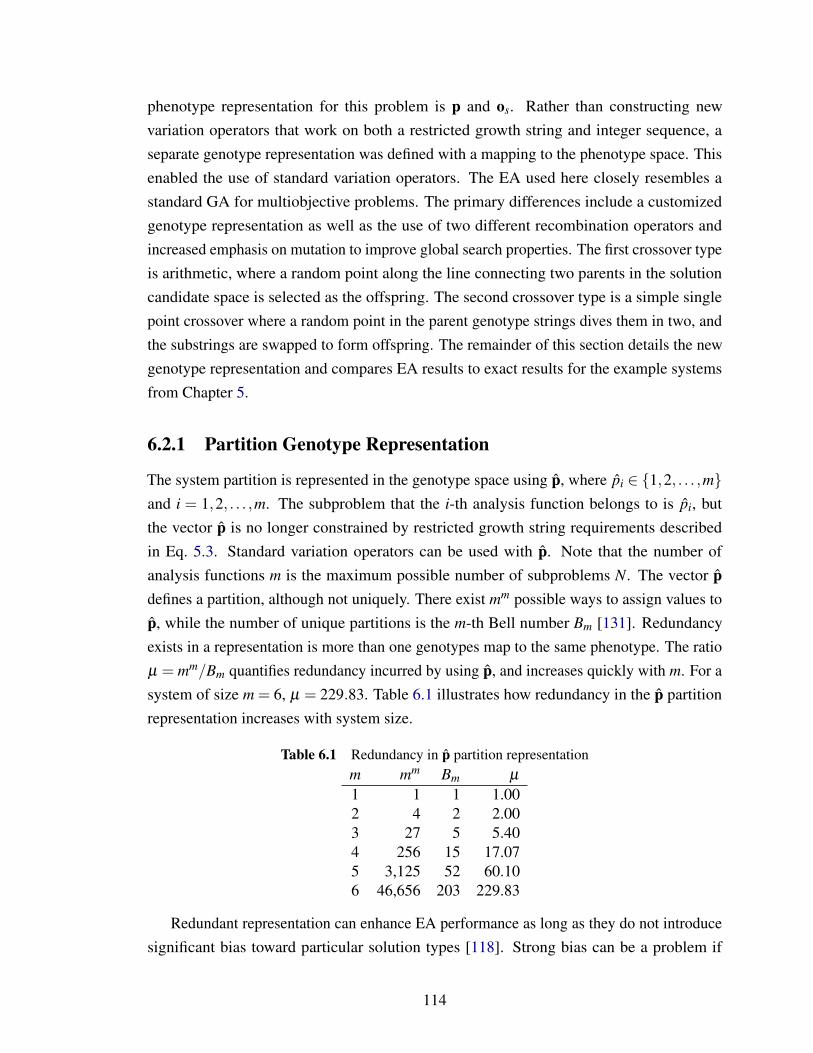
phenotype representation for this problem is p and os. Rather than constructing newvariation operators that work on both a restricted growth string and integer sequence, aseparate genotype representation was defined with a mapping to the phenotype space. Thisenabled the use of standard variation operators. The EA used here closely resembles astandard GA for multiobjective problems. The primary differences include a customizedgenotype representation as well as the use of two different recombination operators andincreased emphasis on mutation to improve global search properties. The first crossover typeis arithmetic, where a random point along the line connecting two parents in the solutioncandidate space is selected as the offspring. The second crossover type is a simple singlepoint crossover where a random point in the parent genotype strings dives them in two, andthe substrings are swapped to form offspring. The remainder of this section details the newgenotype representation and compares EA results to exact results for the example systemsfrom Chapter 5.
6.2.1 Partition Genotype Representation
The system partition is represented in the genotype space using p, where pi ∈ 1,2, . . . ,mand i = 1,2, . . . ,m. The subproblem that the i-th analysis function belongs to is pi, butthe vector p is no longer constrained by restricted growth string requirements describedin Eq. 5.3. Standard variation operators can be used with p. Note that the number ofanalysis functions m is the maximum possible number of subproblems N. The vector pdefines a partition, although not uniquely. There exist mm possible ways to assign values top, while the number of unique partitions is the m-th Bell number Bm [131]. Redundancyexists in a representation is more than one genotypes map to the same phenotype. The ratioµ = mm/Bm quantifies redundancy incurred by using p, and increases quickly with m. For asystem of size m = 6, µ = 229.83. Table 6.1 illustrates how redundancy in the p partitionrepresentation increases with system size.
Table 6.1 Redundancy in p partition representationm mm Bm µ
1 1 1 1.002 4 2 2.003 27 5 5.404 256 15 17.075 3,125 52 60.106 46,656 203 229.83
Redundant representation can enhance EA performance as long as they do not introducesignificant bias toward particular solution types [118]. Strong bias can be a problem if
114
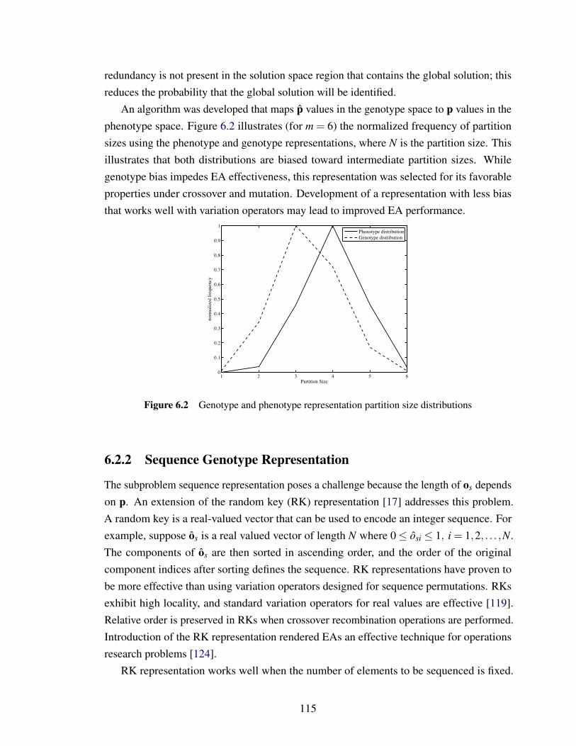
redundancy is not present in the solution space region that contains the global solution; thisreduces the probability that the global solution will be identified.
An algorithm was developed that maps p values in the genotype space to p values in thephenotype space. Figure 6.2 illustrates (for m = 6) the normalized frequency of partitionsizes using the phenotype and genotype representations, where N is the partition size. Thisillustrates that both distributions are biased toward intermediate partition sizes. Whilegenotype bias impedes EA effectiveness, this representation was selected for its favorableproperties under crossover and mutation. Development of a representation with less biasthat works well with variation operators may lead to improved EA performance.
1 2 3 4 5 60
0.1
0.2
0.3
0.4
0.5
0.6
0.7
0.8
0.9
1
Partition Size
norm
aliz
ed f
requen
cy
Phenotype distribution
Genotype distribution
Figure 6.2 Genotype and phenotype representation partition size distributions
6.2.2 Sequence Genotype Representation
The subproblem sequence representation poses a challenge because the length of os dependson p. An extension of the random key (RK) representation [17] addresses this problem.A random key is a real-valued vector that can be used to encode an integer sequence. Forexample, suppose os is a real valued vector of length N where 0≤ osi ≤ 1, i = 1,2, . . . ,N.The components of os are then sorted in ascending order, and the order of the originalcomponent indices after sorting defines the sequence. RK representations have proven tobe more effective than using variation operators designed for sequence permutations. RKsexhibit high locality, and standard variation operators for real values are effective [119].Relative order is preserved in RKs when crossover recombination operations are performed.Introduction of the RK representation rendered EAs an effective technique for operationsresearch problems [124].
RK representation works well when the number of elements to be sequenced is fixed.
115
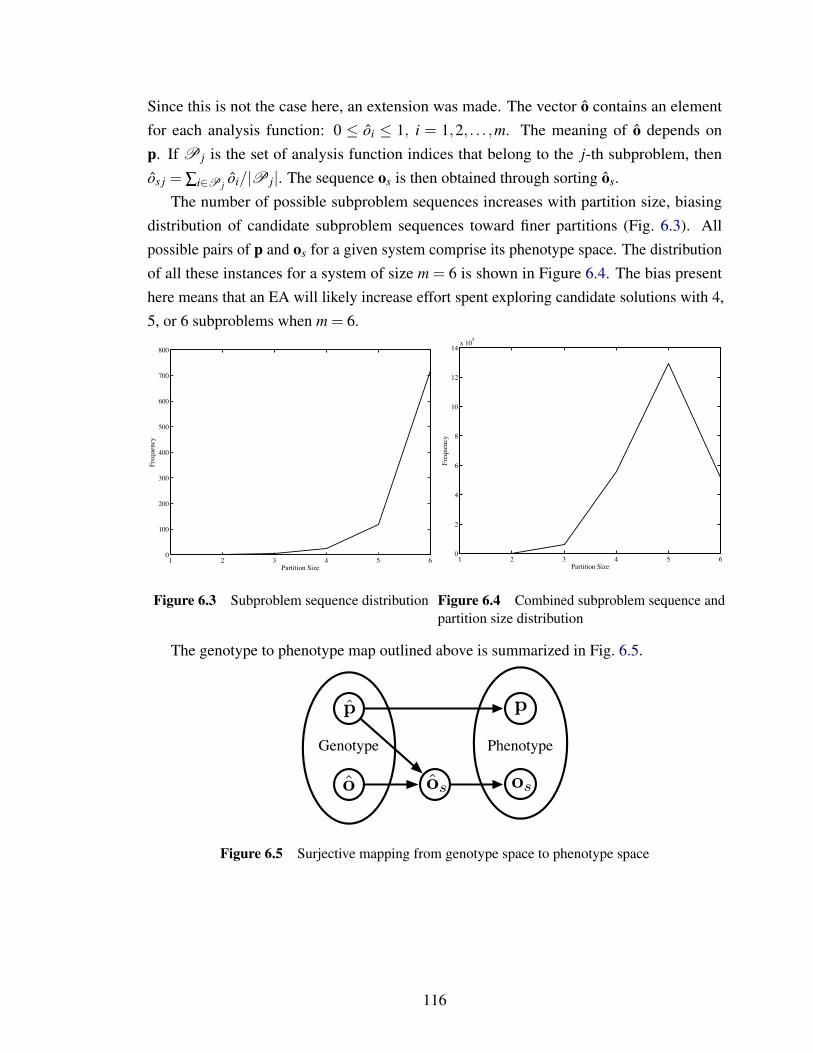
Since this is not the case here, an extension was made. The vector o contains an elementfor each analysis function: 0 ≤ oi ≤ 1, i = 1,2, . . . ,m. The meaning of o depends onp. If P j is the set of analysis function indices that belong to the j-th subproblem, thenos j = ∑i∈P j oi/|P j|. The sequence os is then obtained through sorting os.
The number of possible subproblem sequences increases with partition size, biasingdistribution of candidate subproblem sequences toward finer partitions (Fig. 6.3). Allpossible pairs of p and os for a given system comprise its phenotype space. The distributionof all these instances for a system of size m = 6 is shown in Figure 6.4. The bias presenthere means that an EA will likely increase effort spent exploring candidate solutions with 4,5, or 6 subproblems when m = 6.
1 2 3 4 5 60
100
200
300
400
500
600
700
800
Partition Size
Fre
qu
ency
Figure 6.3 Subproblem sequence distribution
1 2 3 4 5 60
2
4
6
8
10
12
14x 105
Partition Size
Freq
uenc
y
Figure 6.4 Combined subproblem sequence andpartition size distribution
The genotype to phenotype map outlined above is summarized in Fig. 6.5.
problem size (CS) and subproblem sizes (SSi, i ! 1, 2, . . . , N) can be computed using A. Thesesize metrics are proxies for the computational expense associated with solving the coordination problemand subproblems, respectively. CS is the number of consistency constraints that must be solved in thecoordination problem and SSi is the size of the i-th subproblem.
A restricted growth string (RGS) [13] p of length m is used to specify a system partition. Analysisfunction i belongs to the subproblem identified by the value of pi. Redundant representations of partitionsare avoided since, as an RGS, p must satisfy [13]:
p1 = 1 " pi # maxp1, p2, . . . , pi!1 + 1 (1)
The coordination decision model used here is restricted to subproblem sequence choice. A more so-phisticated model that also includes consistency constraint allocation is under development. Subproblemsequence is represented by os, a vector of length N where the value of osi is the evaluation position ofsubproblem i, and osi $= osj , % i, j ! 1, 2, . . . , N.
A simultaneous approach to partitioning and coordination decision-making considers p and os to-gether, rather than independently or in sequence, and can be formulated as a multiobjective optimizationproblem:
minp,os
CS, SSmax, (2)
where SSmax is the maximum subproblem size. Since specification of p and os are coupled tasks, asimultaneous approach is required to obtain Pareto-optimal solutions to Eq. (2).
4. Evolutionary AlgorithmEvolutionary algorithms (EAs) seek to improve the ‘fitness’ of a population composed of candidateproblem solutions through two primary means: selection and variation [14]. A subset of the populationis chosen to produce the population for the next generation using variation operators. This process isrepeated until some termination criterion is met. EAs are particularly e!ective at searching very largedecision spaces and arriving at good, even if not optimal, solutions in a reasonable amount of time. EAshandle multiobjective problems with little additional expense. The discrete decision space of Eq. (2)is vast; the number of possible partitioning and coordination instances increases exponentially with m.The partitioning and sequencing problems are themselves NP -complete and NP -hard, respectively. Anexact solution for the combined problem is possible only for very small systems. It is proposed herethat an EA tailored to the properties of the simultaneous partitioning and coordination problem is ane!ective solution technique for systems of practical size.
In an EA each individual is abstractly represented by its chromosome, or genotype. The genotyperepresentation must be compatible with the variation operators used in the EA. Frequently the repre-sentation of a candidate solution in the original problem statement, also called the phenotype, is notsuitable for use as a genotype representation. In this case an appropriate genotype space must be de-fined along with a surjective mapping onto the phenotype space. Rather than devise variation operatorsthat apply directly to p and os, a genotype compatible with standard crossover and mutation variationoperators was developed.
Choice of genotype representation can strongly influence EA success. An ideal representation shouldnot increase problem di"culty, should enable variation operators to work properly, and should resultin a process that is robust to solution location [15]. To meet these requirements it is important that arepresentation have good locality (i.e., small changes in the genotype space result in small changes inthe phenotype space) and little bias toward particular genotypes.
4.1. Partition Genotype RepresentationRather than attempt to define an e!ective variation operator to operate directly on restricted growthstrings, the system partition is represented in the genotype space using p, where pi ! 1, 2, . . . ,m, i =1, 2, . . . ,m. Note that the number of analysis functions m is the maximum possible number of subprob-lems N . The vector p defines a partition, although not uniquely. There exist mm possible ways toassign values to p, while the number of unique partitions is the m-th Bell number Bm [13]. The ratioµ = mm/Bm quantifies redundancy incurred by using p, and increases quickly with m. For a system ofsize m = 6, µ = 229.83.
3
An algorithm was developed that maps p values in the genotype space to p values in the phenotypespace. Figure 3 illustrates (for m = 6) the normalized frequency of partition sizes using the phenotypeand genotype representations, where N is the partition size. Both distributions are biased towardintermediate values. While genotype bias impedes EA e!ectiveness, this representation was selected forits favorable properties under crossover and mutation.
1 2 3 4 5 60
0.1
0.2
0.3
0.4
0.5
0.6
0.7
0.8
0.9
1
Partition Size
no
rmal
ized
fre
quen
cy
Phenotype distribution
Genotype distribution
Figure 3: Genotype and Phenotype representation partition size distributions
4.2. Sequence Genotype RepresentationThe subproblem sequence representation poses a challenge because the length of os depends on p. Anextension of the Random Key (RK) representation can be utilized to address this problem [16]. A randomkey is a real-valued vector that can be used to encode an integer sequence. For example, suppose os
is a real valued vector of length N where 0 ! osi ! 1, i = 1, 2, . . . , N . The components of os arethen sorted in ascending order, and the order of the original component indices after sorting defines thesequence. RK representations have proven to be more e!ective than using variation operators designedfor permutations. RKs exhibit high locality, and standard variation operators for real values are e!ective[15].
RK representation works well when the number of elements to be sequenced is fixed. Since this isnot the case here, an extension was made. The vector o contains an element for each analysis function:0 ! oi ! 1, i = 1, 2, . . . ,m. The meaning of o depends on p. If Pj is the set of analysis functionindices that belong to the j-th subproblem, then osj =
!i!Pj
oi/|Pj |. The sequence os is then obtainedthrough sorting os.
The number of possible subproblem sequences increases with partition size, biasing distribution ofcandidate subproblem sequences toward finer partitions (Fig. 4). All possible pairs of p and os for agiven system comprise its phenotype space. The distribution of all these instances for a system of sizem = 6 is shown in Figure 5. The bias present here means that an EA will likely expend most of its e!ortexploring candidate solutions with 4, 5, or 6 subproblems.
5. Comparative ExamplesThe exact Pareto-optimal solutions for three small example systems were presented in [11] and arecompared here against results using the EA described above. The first two example systems are definedby the adjacency matrices A1 and A2:
A1 =
"
###$
0 1 1 1 0 1 0 1 1 1 0 10 0 1 1 1 0 1 1 0 1 1 11 0 0 1 1 1 1 1 1 1 1 11 1 1 0 0 1 1 1 1 1 1 11 1 0 1 0 0 1 1 1 0 0 1
%
&&&', A2 =
"
#####$
0 1 1 1 0 0 1 1 1 1 1 1 1 1 0 11 0 1 1 1 0 0 1 1 1 0 1 0 1 1 01 1 0 1 0 1 0 1 0 1 1 1 1 0 1 01 1 1 0 0 0 1 0 1 0 0 1 0 0 0 01 1 1 1 0 0 1 1 1 1 1 1 1 0 1 01 1 1 1 1 0 1 1 1 0 1 1 1 0 1 1
%
&&&&&'.
4
An algorithm was developed that maps p values in the genotype space to p values in the phenotypespace. Figure 3 illustrates (for m = 6) the normalized frequency of partition sizes using the phenotypeand genotype representations, where N is the partition size. Both distributions are biased towardintermediate values. While genotype bias impedes EA e!ectiveness, this representation was selected forits favorable properties under crossover and mutation.
1 2 3 4 5 60
0.1
0.2
0.3
0.4
0.5
0.6
0.7
0.8
0.9
1
Partition Size
norm
aliz
ed f
requen
cy
Phenotype distribution
Genotype distribution
Figure 3: Genotype and Phenotype representation partition size distributions
4.2. Sequence Genotype RepresentationThe subproblem sequence representation poses a challenge because the length of os depends on p. Anextension of the Random Key (RK) representation can be utilized to address this problem [16]. A randomkey is a real-valued vector that can be used to encode an integer sequence. For example, suppose os
is a real valued vector of length N where 0 ! osi ! 1, i = 1, 2, . . . , N . The components of os arethen sorted in ascending order, and the order of the original component indices after sorting defines thesequence. RK representations have proven to be more e!ective than using variation operators designedfor permutations. RKs exhibit high locality, and standard variation operators for real values are e!ective[15].
RK representation works well when the number of elements to be sequenced is fixed. Since this isnot the case here, an extension was made. The vector o contains an element for each analysis function:0 ! oi ! 1, i = 1, 2, . . . ,m. The meaning of o depends on p. If Pj is the set of analysis functionindices that belong to the j-th subproblem, then osj =
!i!Pj
oi/|Pj |. The sequence os is then obtainedthrough sorting os.
The number of possible subproblem sequences increases with partition size, biasing distribution ofcandidate subproblem sequences toward finer partitions (Fig. 4). All possible pairs of p and os for agiven system comprise its phenotype space. The distribution of all these instances for a system of sizem = 6 is shown in Figure 5. The bias present here means that an EA will likely expend most of its e!ortexploring candidate solutions with 4, 5, or 6 subproblems.
5. Comparative ExamplesThe exact Pareto-optimal solutions for three small example systems were presented in [11] and arecompared here against results using the EA described above. The first two example systems are definedby the adjacency matrices A1 and A2:
A1 =
"
###$
0 1 1 1 0 1 0 1 1 1 0 10 0 1 1 1 0 1 1 0 1 1 11 0 0 1 1 1 1 1 1 1 1 11 1 1 0 0 1 1 1 1 1 1 11 1 0 1 0 0 1 1 1 0 0 1
%
&&&', A2 =
"
#####$
0 1 1 1 0 0 1 1 1 1 1 1 1 1 0 11 0 1 1 1 0 0 1 1 1 0 1 0 1 1 01 1 0 1 0 1 0 1 0 1 1 1 1 0 1 01 1 1 0 0 0 1 0 1 0 0 1 0 0 0 01 1 1 1 0 0 1 1 1 1 1 1 1 0 1 01 1 1 1 1 0 1 1 1 0 1 1 1 0 1 1
%
&&&&&'.
4
problem size (CS) and subproblem sizes (SSi, i ! 1, 2, . . . , N) can be computed using A. Thesesize metrics are proxies for the computational expense associated with solving the coordination problemand subproblems, respectively. CS is the number of consistency constraints that must be solved in thecoordination problem and SSi is the size of the i-th subproblem.
A restricted growth string (RGS) [13] p of length m is used to specify a system partition. Analysisfunction i belongs to the subproblem identified by the value of pi. Redundant representations of partitionsare avoided since, as an RGS, p must satisfy [13]:
p1 = 1 " pi # maxp1, p2, . . . , pi!1 + 1 (1)
The coordination decision model used here is restricted to subproblem sequence choice. A more so-phisticated model that also includes consistency constraint allocation is under development. Subproblemsequence is represented by os, a vector of length N where the value of osi is the evaluation position ofsubproblem i, and osi $= osj , % i, j ! 1, 2, . . . , N.
A simultaneous approach to partitioning and coordination decision-making considers p and os to-gether, rather than independently or in sequence, and can be formulated as a multiobjective optimizationproblem:
minp,os
CS, SSmax, (2)
where SSmax is the maximum subproblem size. Since specification of p and os are coupled tasks, asimultaneous approach is required to obtain Pareto-optimal solutions to Eq. (2).
4. Evolutionary AlgorithmEvolutionary algorithms (EAs) seek to improve the ‘fitness’ of a population composed of candidateproblem solutions through two primary means: selection and variation [14]. A subset of the populationis chosen to produce the population for the next generation using variation operators. This process isrepeated until some termination criterion is met. EAs are particularly e!ective at searching very largedecision spaces and arriving at good, even if not optimal, solutions in a reasonable amount of time. EAshandle multiobjective problems with little additional expense. The discrete decision space of Eq. (2)is vast; the number of possible partitioning and coordination instances increases exponentially with m.The partitioning and sequencing problems are themselves NP -complete and NP -hard, respectively. Anexact solution for the combined problem is possible only for very small systems. It is proposed herethat an EA tailored to the properties of the simultaneous partitioning and coordination problem is ane!ective solution technique for systems of practical size.
In an EA each individual is abstractly represented by its chromosome, or genotype. The genotyperepresentation must be compatible with the variation operators used in the EA. Frequently the repre-sentation of a candidate solution in the original problem statement, also called the phenotype, is notsuitable for use as a genotype representation. In this case an appropriate genotype space must be de-fined along with a surjective mapping onto the phenotype space. Rather than devise variation operatorsthat apply directly to p and os, a genotype compatible with standard crossover and mutation variationoperators was developed.
Choice of genotype representation can strongly influence EA success. An ideal representation shouldnot increase problem di"culty, should enable variation operators to work properly, and should resultin a process that is robust to solution location [15]. To meet these requirements it is important that arepresentation have good locality (i.e., small changes in the genotype space result in small changes inthe phenotype space) and little bias toward particular genotypes.
4.1. Partition Genotype RepresentationRather than attempt to define an e!ective variation operator to operate directly on restricted growthstrings, the system partition is represented in the genotype space using p, where pi ! 1, 2, . . . ,m, i =1, 2, . . . ,m. Note that the number of analysis functions m is the maximum possible number of subprob-lems N . The vector p defines a partition, although not uniquely. There exist mm possible ways toassign values to p, while the number of unique partitions is the m-th Bell number Bm [13]. The ratioµ = mm/Bm quantifies redundancy incurred by using p, and increases quickly with m. For a system ofsize m = 6, µ = 229.83.
3
PhenotypeGenotype
Figure 6.5 Surjective mapping from genotype space to phenotype space
116
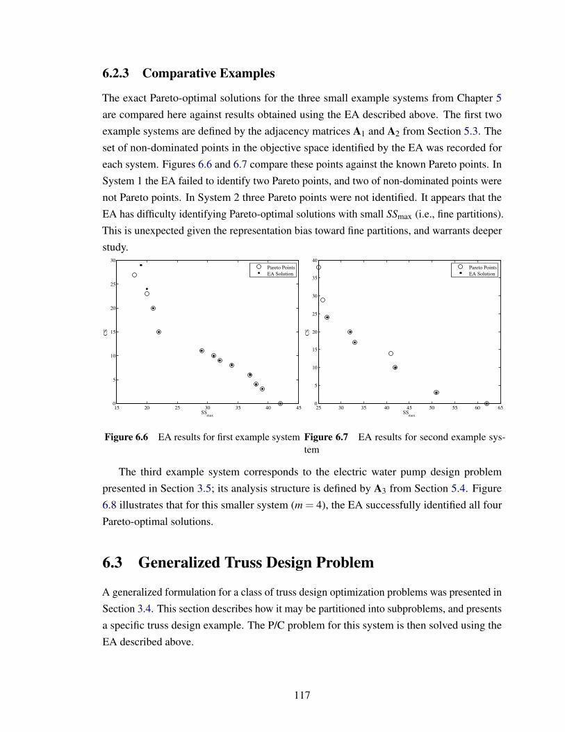
6.2.3 Comparative Examples
The exact Pareto-optimal solutions for the three small example systems from Chapter 5are compared here against results obtained using the EA described above. The first twoexample systems are defined by the adjacency matrices A1 and A2 from Section 5.3. Theset of non-dominated points in the objective space identified by the EA was recorded foreach system. Figures 6.6 and 6.7 compare these points against the known Pareto points. InSystem 1 the EA failed to identify two Pareto points, and two of non-dominated points werenot Pareto points. In System 2 three Pareto points were not identified. It appears that theEA has difficulty identifying Pareto-optimal solutions with small SSmax (i.e., fine partitions).This is unexpected given the representation bias toward fine partitions, and warrants deeperstudy.
15 20 25 30 35 40 450
5
10
15
20
25
30
SSmax
CS
Pareto PointsEA Solution
Figure 6.6 EA results for first example system
25 30 35 40 45 50 55 60 650
5
10
15
20
25
30
35
40
SSmax
CS
Pareto PointsEA Solution
Figure 6.7 EA results for second example sys-tem
The third example system corresponds to the electric water pump design problempresented in Section 3.5; its analysis structure is defined by A3 from Section 5.4. Figure6.8 illustrates that for this smaller system (m = 4), the EA successfully identified all fourPareto-optimal solutions.
6.3 Generalized Truss Design Problem
A generalized formulation for a class of truss design optimization problems was presented inSection 3.4. This section describes how it may be partitioned into subproblems, and presentsa specific truss design example. The P/C problem for this system is then solved using theEA described above.
117
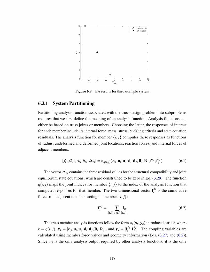
12 14 16 18 20 22 24 26 280
2
4
6
8
10
12
SSmax
CS
Pareto PointsEA Solution
Figure 6.8 EA results for third example system
6.3.1 System Partitioning
Partitioning analysis function associated with the truss design problem into subproblemsrequires that we first define the meaning of an analysis function. Analysis functions caneither be based on truss joints or members. Choosing the latter, the responses of interestfor each member include its internal force, mass, stress, buckling criteria and state equationresiduals. The analysis function for member i, j computes these responses as functionsof radius, undeformed and deformed joint locations, reaction forces, and internal forces ofadjacent members:
[ fi j,Ωi j,σi j,bi j,∆i j] = aq(i, j)(ri j,ui,u j,di,d j,Ri,R j, fi ji , f i j
j ) (6.1)
The vector ∆i j contains the three residual values for the structural compatibility and jointequilibrium state equations, which are constrained to be zero in Eq. (3.29). The functionq(i, j) maps the joint indices for member i, j to the index of the analysis function thatcomputes responses for that member. The two-dimensional vector f i j
i is the cumulativeforce from adjacent members acting on member i, j:
f i ji = ∑
i,k∈Ai\i, jfik (6.2)
The truss member analysis functions follow the form ak(xk,yk) introduced earlier, wherek = q(i, j), xk = [ri j,ui,u j,di,d j,Ri,R j], and yk = [f i j
i , f i jj ]. The coupling variables are
calculated using member force values and geometry information (Eqs. (3.27) and (6.2)).Since fi j is the only analysis output required by other analysis functions, it is the only
118

coupling variable, and is of prime interest when making partitioning and coordinationdecisions for the partitioned truss design problem. All other analysis outputs are localquantities.
These analysis functions can be clustered to form subproblems. If we use IDF-typesubproblem formulations, when members in different subproblems are connected at commonjoints, the corresponding internal member forces are coupling variables between the sub-problems. In addition, undeformed positions of common joints are shared decision variables.Deformed locations and reaction forces for common joints are also shared variables since thestate variables di and Ri are treated as design variables. The objective function is additivelyseparable, enabling the formation of local subproblem objective functions that consist of themass of all members in a subproblem.
A wide variety of analysis structures and system sizes are available using this formulationdepending on truss size and topology, making Eq. (3.29) a suitable platform for testing theperformance of decomposition-based design optimization methods, as well as methods forcombined partition and coordination decision-making.
6.3.2 Example: Eight-bar Truss
An eight-bar truss problem with topology adopted from [62] was formulated, partitioned,and solved for use in demonstrating the evolutionary algorithm on a system too large for anexhaustive enumeration approach to making P/C decisions. This truss is illustrated in Fig.6.9.
1
2 3
4
5
F3
6
F6
x
y
Figure 6.9 Geometry and applied loads for the 8-bar truss problem
The member radii values are r = [r14,r24,r23,r34,r45,r35,r36,r56], the movable joint po-sitions are m = [u4,u5], the deformed positions of non-ground joints are d = [d3,d4,d5,d6],and the reaction forces are R = [R1,R2]. The reduced adjacency matrix for this system
119
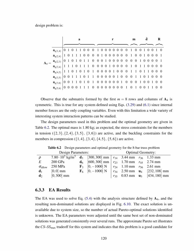
design problem is:
A4 =
a r m d R︷ ︸︸ ︷ ︷ ︸︸ ︷ ︷︸︸︷ ︷ ︸︸ ︷ ︷︸︸︷aq(1,4) 0 1 0 1 1 0 0 0 1 0 0 0 0 0 0 0 1 0 0 1 0 0 1 0
aq(2,4) 1 0 1 1 1 0 0 0 0 1 0 0 0 0 0 0 1 0 0 1 0 0 0 1
aq(2,3) 0 1 0 1 0 1 1 0 0 0 1 0 0 0 0 0 0 0 1 0 0 0 0 1
aq(3,4) 1 1 1 0 1 1 1 0 0 0 0 1 0 0 0 0 1 0 1 1 0 0 0 0
aq(4,5) 1 1 0 1 0 1 0 1 0 0 0 0 1 0 0 0 1 1 0 1 1 0 0 0
aq(3,5) 0 0 1 1 1 0 1 1 0 0 0 0 0 1 0 0 0 1 1 0 1 0 0 0
aq(3,6) 0 0 1 1 0 1 0 1 0 0 0 0 0 0 1 0 0 0 1 0 0 1 0 0
aq(5,6) 0 0 0 0 1 1 1 0 0 0 0 0 0 0 0 1 0 1 0 0 1 1 0 0
Observe that the submatrix formed by the first m = 8 rows and columns of A4 issymmetric. This is true for any system defined using Eqs. (3.29) and (6.1) since internalmember forces are the only coupling variables. Even with this limitation a wide variety ofinteresting system interaction patterns can be studied.
The design parameters used in this problem and the optimal geometry are given inTable 6.2. The optimal mass is 1.80 kg; as expected, the stress constraints for the membersin tension (2,3,2,4,3,5, 3,6) are active, and the buckling constraints for themembers in compression (1,4,3,4,4,5, 5,6) are active.
Table 6.2 Design parameters and optimal geometry for the 8-bar truss problemDesign Parameters: Optimal Geometry:
ρ 7.80 ·103 kg/m3 d3 [300,300] mm r14 3.44 mm r36 1.33 mmE 200 GPa d6 [600,300] mm r23 1.70 mm r45 2.74 mmσallow 250 MPa F3 [0,−1000] N r24 1.10 mm r56 2.61 mmd1 [0,0] mm F6 [0,−1000] N r34 2.50 mm u4 [232,108] mmd2 [0,300] mm r35 0.83 mm u5 [434,180] mm
6.3.3 EA Results
The EA was used to solve Eq. (5.4) with the analysis structure defined by A4, and theresulting non-dominated solutions are displayed in Fig. 6.10. The exact solution is un-available due to system size, so the number of actual Pareto-optimal solutions identifiedis unknown. The EA parameters were adjusted until the same best set of non-dominatedsolutions was generated consistently over several runs. The approximate Pareto set illustratesthe CS–SSmax tradeoff for this system and indicates that this problem is a good candidate for
120
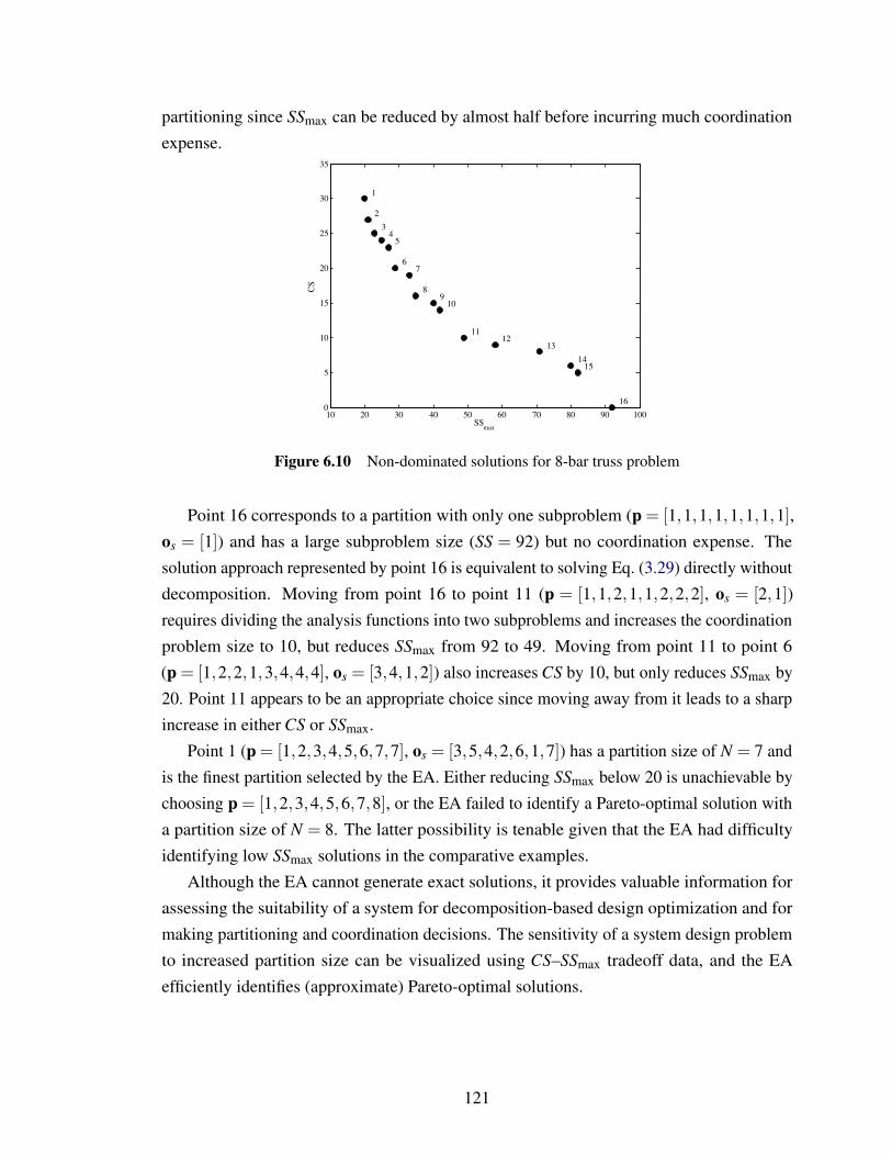
partitioning since SSmax can be reduced by almost half before incurring much coordinationexpense.
10 20 30 40 50 60 70 80 90 1000
5
10
15
20
25
30
35
SSmax
CS
1
2345
67
8910
1112
131415
16
Figure 6.10 Non-dominated solutions for 8-bar truss problem
Point 16 corresponds to a partition with only one subproblem (p = [1,1,1,1,1,1,1,1],os = [1]) and has a large subproblem size (SS = 92) but no coordination expense. Thesolution approach represented by point 16 is equivalent to solving Eq. (3.29) directly withoutdecomposition. Moving from point 16 to point 11 (p = [1,1,2,1,1,2,2,2], os = [2,1])requires dividing the analysis functions into two subproblems and increases the coordinationproblem size to 10, but reduces SSmax from 92 to 49. Moving from point 11 to point 6(p = [1,2,2,1,3,4,4,4], os = [3,4,1,2]) also increases CS by 10, but only reduces SSmax by20. Point 11 appears to be an appropriate choice since moving away from it leads to a sharpincrease in either CS or SSmax.
Point 1 (p = [1,2,3,4,5,6,7,7], os = [3,5,4,2,6,1,7]) has a partition size of N = 7 andis the finest partition selected by the EA. Either reducing SSmax below 20 is unachievable bychoosing p = [1,2,3,4,5,6,7,8], or the EA failed to identify a Pareto-optimal solution witha partition size of N = 8. The latter possibility is tenable given that the EA had difficultyidentifying low SSmax solutions in the comparative examples.
Although the EA cannot generate exact solutions, it provides valuable information forassessing the suitability of a system for decomposition-based design optimization and formaking partitioning and coordination decisions. The sensitivity of a system design problemto increased partition size can be visualized using CS–SSmax tradeoff data, and the EAefficiently identifies (approximate) Pareto-optimal solutions.
121
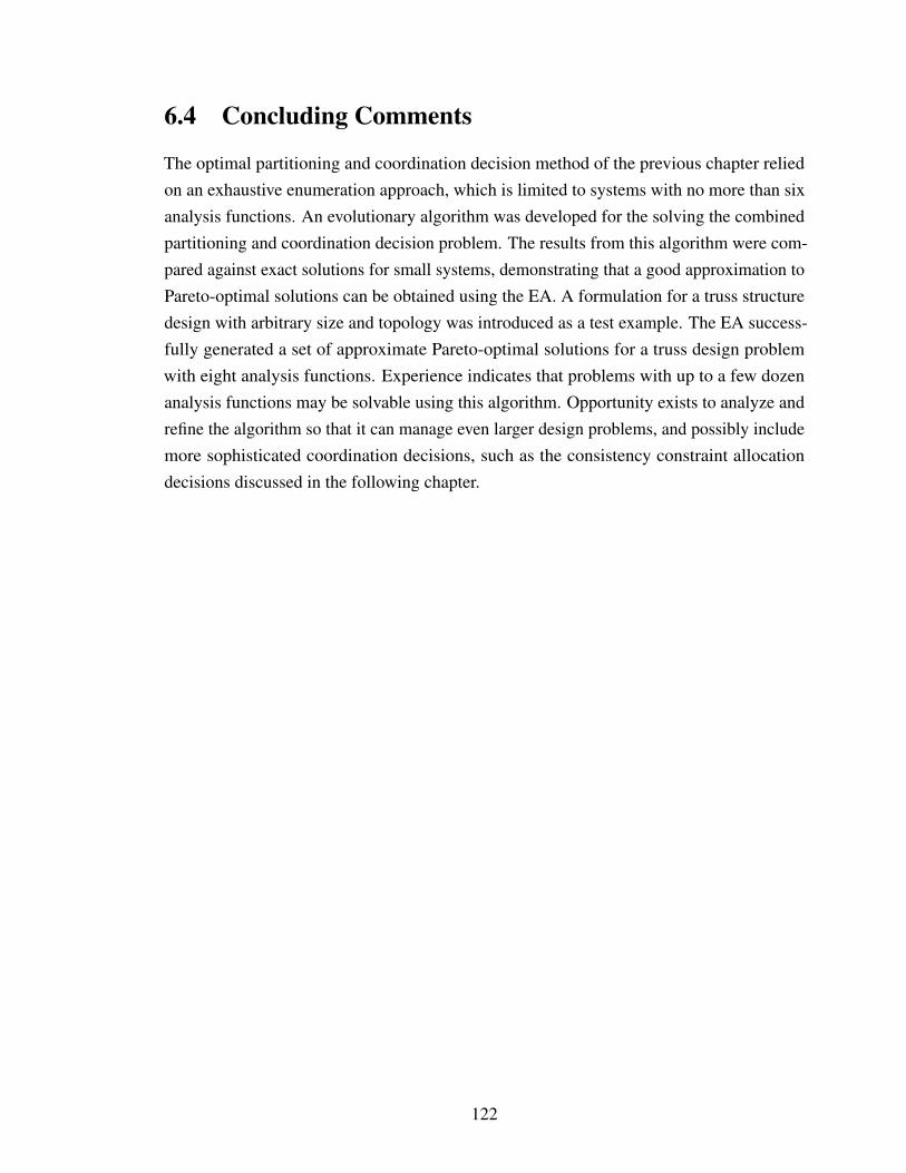
6.4 Concluding Comments
The optimal partitioning and coordination decision method of the previous chapter reliedon an exhaustive enumeration approach, which is limited to systems with no more than sixanalysis functions. An evolutionary algorithm was developed for the solving the combinedpartitioning and coordination decision problem. The results from this algorithm were com-pared against exact solutions for small systems, demonstrating that a good approximation toPareto-optimal solutions can be obtained using the EA. A formulation for a truss structuredesign with arbitrary size and topology was introduced as a test example. The EA success-fully generated a set of approximate Pareto-optimal solutions for a truss design problemwith eight analysis functions. Experience indicates that problems with up to a few dozenanalysis functions may be solvable using this algorithm. Opportunity exists to analyze andrefine the algorithm so that it can manage even larger design problems, and possibly includemore sophisticated coordination decisions, such as the consistency constraint allocationdecisions discussed in the following chapter.
122

Chapter 7
Consistency Constraint Allocation for AugmentedLagrangian Coordination
The Augmented Lagrangian Coordination (ALC) formulation, presented in Section 4.3.4,provides significant flexibility in problem linking structure. The way consistency constraintsare allocated among subproblems defines ALC linking structure. While the ability to tailorlinking structure to a particular problem can be a profound benefit, manually sifting throughthe numerous options for linking structure is an overwhelming task. This chapter developsthe theory necessary to understand linking structure options for ALC, and shows how toinclude linking structure decisions along with subproblem sequence decisions in an optimalP/C decision approach for ALC. This is illustrated using a parallel version of ALC.
Techniques from constraint satisfaction programming are used to analyze linking struc-ture for ALC. Graph theory is used to represent the structure of consistency constraintsin an ALC formulation. An undirected graph, called the consistency constraint graph, isdefined for every linking variable. It is shown that a set of consistency constraints for alinking variable in ALC is valid if and only if the corresponding consistency constraintgraph is a spanning tree1. This important result means that set of all possible ALC linkingstructure options for a system design problem can be defined, allowing the inclusion oflinking structure decisions in the optimal partitioning and coordination decision problem forALC. A method for solving this problem is described in detail, and demonstrated using theelectric water pump design problem from Section 3.5.1.
7.1 Parallel ALC
This section introduces a new approach to formulating ALC problems for parallel compu-tations where the number of subproblems exceeds the number of processors. An examplesystem with six analysis functions is used to illustrate concepts:
1A graph is a spanning tree if it is connected and contains no cycles.
123
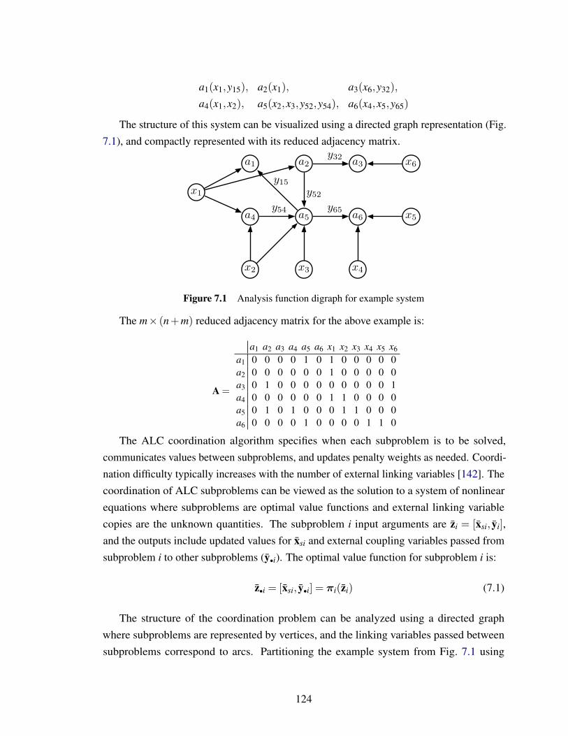
a1(x1,y15), a2(x1), a3(x6,y32),a4(x1,x2), a5(x2,x3,y52,y54), a6(x4,x5,y65)
The structure of this system can be visualized using a directed graph representation (Fig.7.1), and compactly represented with its reduced adjacency matrix.
a1 a2 a3
a4
x1
x2 x3 x4
a5 a6
y15
y54
y52
y65
y32
x5
x6
Figure 7.1 Analysis function digraph for example system
The m× (n+m) reduced adjacency matrix for the above example is:
A =
a1 a2 a3 a4 a5 a6 x1 x2 x3 x4 x5 x6
a1 0 0 0 0 1 0 1 0 0 0 0 0a2 0 0 0 0 0 0 1 0 0 0 0 0a3 0 1 0 0 0 0 0 0 0 0 0 1a4 0 0 0 0 0 0 1 1 0 0 0 0a5 0 1 0 1 0 0 0 1 1 0 0 0a6 0 0 0 0 1 0 0 0 0 1 1 0
The ALC coordination algorithm specifies when each subproblem is to be solved,communicates values between subproblems, and updates penalty weights as needed. Coordi-nation difficulty typically increases with the number of external linking variables [142]. Thecoordination of ALC subproblems can be viewed as the solution to a system of nonlinearequations where subproblems are optimal value functions and external linking variablecopies are the unknown quantities. The subproblem i input arguments are zi = [xsi, yi],and the outputs include updated values for xsi and external coupling variables passed fromsubproblem i to other subproblems (y•i). The optimal value function for subproblem i is:
z•i = [xsi, y•i] = πi(zi) (7.1)
The structure of the coordination problem can be analyzed using a directed graphwhere subproblems are represented by vertices, and the linking variables passed betweensubproblems correspond to arcs. Partitioning the example system from Fig. 7.1 using
124
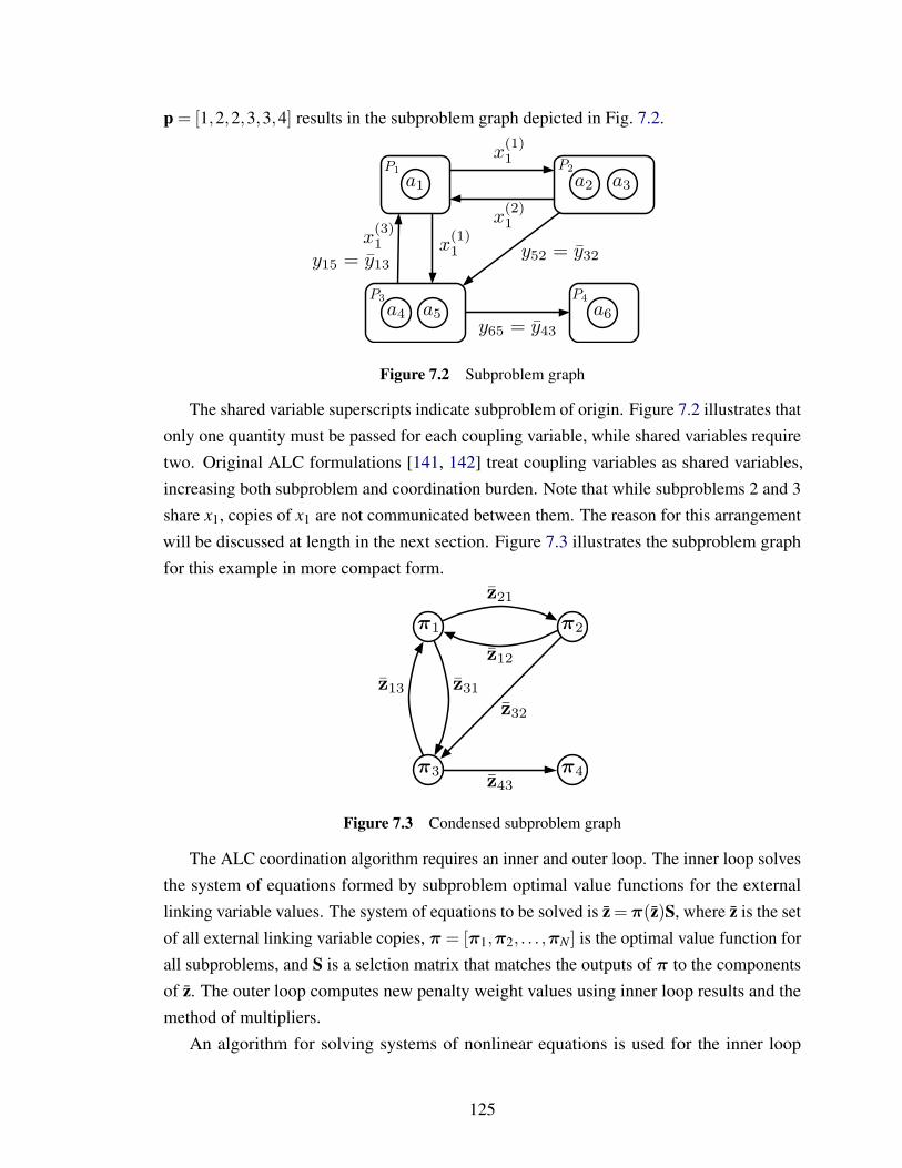
p = [1,2,2,3,3,4] results in the subproblem graph depicted in Fig. 7.2.
a1 a2 a3
a4 a5 a6
P1P2
P3 P4
x(2)1
x(1)1
x(1)1
x(3)1
y65 = y43
y52 = y32y15 = y13
Figure 7.2 Subproblem graph
The shared variable superscripts indicate subproblem of origin. Figure 7.2 illustrates thatonly one quantity must be passed for each coupling variable, while shared variables requiretwo. Original ALC formulations [141, 142] treat coupling variables as shared variables,increasing both subproblem and coordination burden. Note that while subproblems 2 and 3share x1, copies of x1 are not communicated between them. The reason for this arrangementwill be discussed at length in the next section. Figure 7.3 illustrates the subproblem graphfor this example in more compact form.
!1 !2
!3 !4
z21
z12
z13 z31
z32
z43
Figure 7.3 Condensed subproblem graph
The ALC coordination algorithm requires an inner and outer loop. The inner loop solvesthe system of equations formed by subproblem optimal value functions for the externallinking variable values. The system of equations to be solved is z = π(z)S, where z is the setof all external linking variable copies, π = [π1,π2, . . . ,πN ] is the optimal value function forall subproblems, and S is a selction matrix that matches the outputs of π to the componentsof z. The outer loop computes new penalty weight values using inner loop results and themethod of multipliers.
An algorithm for solving systems of nonlinear equations is used for the inner loop
125
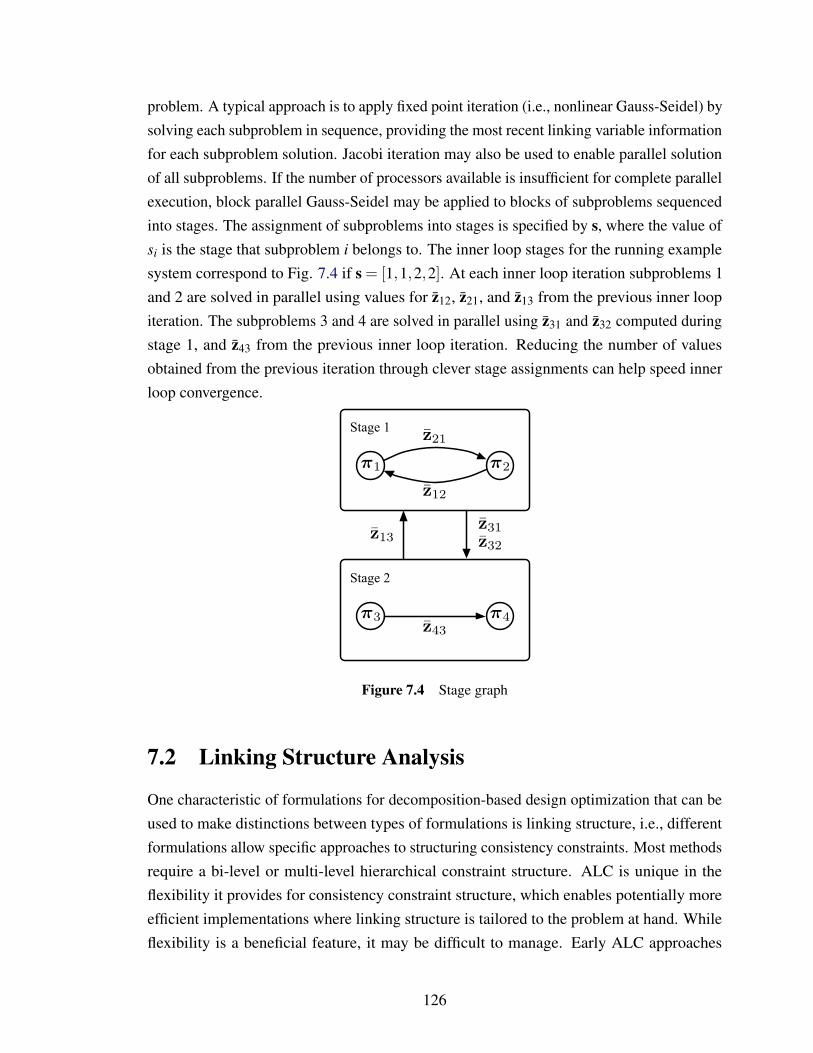
problem. A typical approach is to apply fixed point iteration (i.e., nonlinear Gauss-Seidel) bysolving each subproblem in sequence, providing the most recent linking variable informationfor each subproblem solution. Jacobi iteration may also be used to enable parallel solutionof all subproblems. If the number of processors available is insufficient for complete parallelexecution, block parallel Gauss-Seidel may be applied to blocks of subproblems sequencedinto stages. The assignment of subproblems into stages is specified by s, where the value ofsi is the stage that subproblem i belongs to. The inner loop stages for the running examplesystem correspond to Fig. 7.4 if s = [1,1,2,2]. At each inner loop iteration subproblems 1and 2 are solved in parallel using values for z12, z21, and z13 from the previous inner loopiteration. The subproblems 3 and 4 are solved in parallel using z31 and z32 computed duringstage 1, and z43 from the previous inner loop iteration. Reducing the number of valuesobtained from the previous iteration through clever stage assignments can help speed innerloop convergence.
!1 !2
!3 !4
z21
z12
z13
z31
z32
z43
Stage 1
Stage 2
Figure 7.4 Stage graph
7.2 Linking Structure Analysis
One characteristic of formulations for decomposition-based design optimization that can beused to make distinctions between types of formulations is linking structure, i.e., differentformulations allow specific approaches to structuring consistency constraints. Most methodsrequire a bi-level or multi-level hierarchical constraint structure. ALC is unique in theflexibility it provides for consistency constraint structure, which enables potentially moreefficient implementations where linking structure is tailored to the problem at hand. Whileflexibility is a beneficial feature, it may be difficult to manage. Early ALC approaches
126
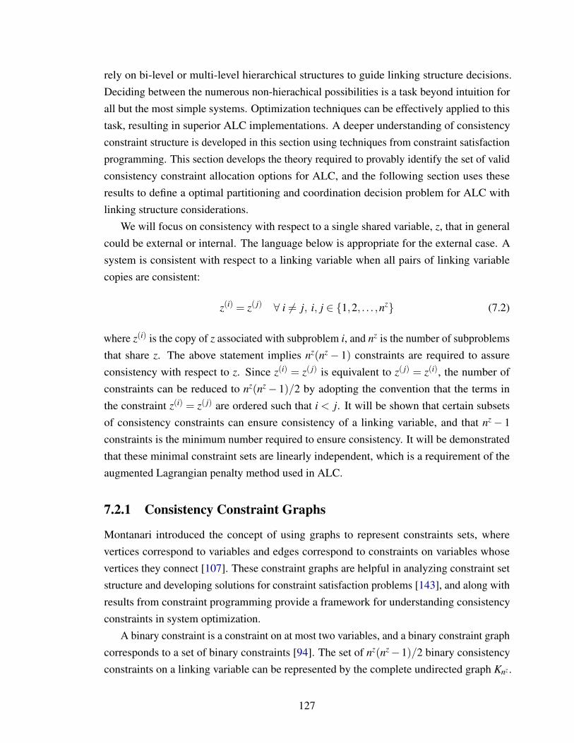
rely on bi-level or multi-level hierarchical structures to guide linking structure decisions.Deciding between the numerous non-hierachical possibilities is a task beyond intuition forall but the most simple systems. Optimization techniques can be effectively applied to thistask, resulting in superior ALC implementations. A deeper understanding of consistencyconstraint structure is developed in this section using techniques from constraint satisfactionprogramming. This section develops the theory required to provably identify the set of validconsistency constraint allocation options for ALC, and the following section uses theseresults to define a optimal partitioning and coordination decision problem for ALC withlinking structure considerations.
We will focus on consistency with respect to a single shared variable, z, that in generalcould be external or internal. The language below is appropriate for the external case. Asystem is consistent with respect to a linking variable when all pairs of linking variablecopies are consistent:
z(i) = z( j) ∀ i 6= j, i, j ∈ 1,2, . . . ,nz (7.2)
where z(i) is the copy of z associated with subproblem i, and nz is the number of subproblemsthat share z. The above statement implies nz(nz− 1) constraints are required to assureconsistency with respect to z. Since z(i) = z( j) is equivalent to z( j) = z(i), the number ofconstraints can be reduced to nz(nz− 1)/2 by adopting the convention that the terms inthe constraint z(i) = z( j) are ordered such that i < j. It will be shown that certain subsetsof consistency constraints can ensure consistency of a linking variable, and that nz− 1constraints is the minimum number required to ensure consistency. It will be demonstratedthat these minimal constraint sets are linearly independent, which is a requirement of theaugmented Lagrangian penalty method used in ALC.
7.2.1 Consistency Constraint Graphs
Montanari introduced the concept of using graphs to represent constraints sets, wherevertices correspond to variables and edges correspond to constraints on variables whosevertices they connect [107]. These constraint graphs are helpful in analyzing constraint setstructure and developing solutions for constraint satisfaction problems [143], and along withresults from constraint programming provide a framework for understanding consistencyconstraints in system optimization.
A binary constraint is a constraint on at most two variables, and a binary constraint graphcorresponds to a set of binary constraints [94]. The set of nz(nz−1)/2 binary consistencyconstraints on a linking variable can be represented by the complete undirected graph Knz .
127
An edge i, j represents the constraint z(i) = z( j), which can be expressed in negative nullform as z(i)− z( j) = 0. A convenient representation of this constraint is:
θi jzT = 0 (7.3)
where θi j is the constraint vector that corresponds to edge i, j, and z is the vector of all nz
copies of the linking variable z. More precisely:
θi j = ei− e j (7.4)
z =[z(1),z(2), . . . ,z(nz)
](7.5)
where ei is the ith unit vector of length nz. Two constraints are adjacent if their correspondingconstraint graph edges are adjacent (i.e., they share a common variable). A consistencyconstraint graph Gc is defined as a subgraph of Knz that corresponds to a subset of the nz(nz−1)/2 consistency constraints. The consistency constraint matrix Θ for Gc is composed ofall constraint vectors θi j that correspond to edges in Gc. The edges in Gc specify whichconsistency constraints are to be used in an ALC solution process.
7.2.2 Valid Consistency Constraint Graphs
Not every possible consistency constraint graph is valid for use with ALC. A consistencyconstraint graph is valid if its associated constraints are equivalent to the constraints specifiedby Knz , and if the rows of the corresponding Θ are linearly independent. The first requirementensures complete consistency of the associated linking variable and the second is necessaryfor the success of the augmented Lagrangian penalty method used in ALC. After thedevelopment of preliminary concepts, necessary and sufficient conditions for the validity ofconstraint graphs will be given.
Two sets of constraints are equivalent if their feasible domains are equal. The task offinding reduced sets of constraints equivalent to some original set is known as problemreduction. A constraint is redundant if its removal does not change the feasible domain ofa constraint set. The composition of adjacent constraints can induce implicit constraints.A constraint is said to be explicit if its corresponding edge exists in Gc, and implicit ifit does not. Gc contains redundant constraints if any implicit constraints are identical toeither explicit constraints or other implicit constraints [143]. The properties of consistencyconstraint graphs enable easy identification of implicit and redundant constraints for thepurpose of problem reduction. A consistency constraint graph is minimal if it specifies the
128
fewest number of constraints required to ensure consistency.Identification of implicit constraints requires application of a binary operator called
constraint composition that generates a new constraint from two adjacent constraints [94].
Definition Let γ1(i, j) and γ2( j,k) be two binary constraints with a common variable(z( j))
corresponding to vertex j, and let their composition be γc(i,k). A binary constraint
composition is valid if values for z(i) and z(k) satisfy γc(i,k) if and only if there exists a valueof z( j) such that γ1(i, j) and γ2( j,k) are satisfied.
In a consistency constraint graph two constraints with a common variable can be com-posed to form an implicit constraint by taking the vector sum of the corresponding constraintvectors.
Proposition 7.2.1 The composition of the consistency constraints defined by θi j and θ jk
with the common variable z( j) is θik = θi j +θ jk = ei− e j + e j− ek = ei− ek.
Proof Let ai and ak be values for z(i) and z(k), respectively, such that θikzT = 0 is satisfied.By definition of θik, ai = ak. By selecting a value a j for z( j) such that ai = a j = ak, theconstraints θi jzT = 0 and θ jkzT = 0 consequently are satisfied. Let bi, b j, and bk be valuesfor z(i), z( j), and z(k), respectively, that satisfy θi jzT = 0 and θ jkzT = 0. Since this satisfactionimplies bi = b j and b j = bk, bi = bk and the composed constraint θikzT = 0 is satisfied.Therefore, θik = θi j +θ jk is a valid constraint composition.
A higher than binary constraint composition is defined by the recursive application of abinary constraint composition. Binary consistency constraints that share a common variablehave corresponding edges that are incident to the common variable vertex. At each stage ofrecursive composition a new edge can be included in the composition if it has a commonvertex with the implicit edge generated by the intermediate composition. This occurs whenall edges in a set to be composed lie in a connected path on Gc. Suppose pi j is a connectedpath of length m between the vertices i and j defined by the sequence of unique vertices〈v1,v2, . . . ,vm,vm+1〉 where v1 = i and vm+1 = j. The constraint vector resulting from theextended composition of edges in pi j is θi j = ∑k,l∈pi j θkl = ei− e j.
Proposition 7.2.2 A constraint defined by θi j, whether implicit or explicit, can be obtained
through composition if and only if a path pi j exists in Gc.
129
Proof If a path pi j exists in Gc, extended constraint composition can be applied to obtainθi j:
θi j = ∑k,l∈pi j
θkl
= ev1− ev2 + ev2− ev3 + . . .+ evm− evm+1
=m
∑k=1
evk−m+1
∑k=2
evk (7.6)
= ev1 +m
∑k=2
evk−m
∑k=2
evk− evm+1
= ev1− evm+1 = ei− e j
If a path pi j does not exist in Gc, then at least one edge k, l in every possible set ofconstraint edges will be pendant2. If k is the pendant vertex, θkl will contribute ek to theconstraint composition. Since only edge k, l is adjacent to k, no constraint vector in thecomposition can annihilate ek. The case for l pendant is similar. Therefore, θi j = ei− e j
cannot be obtained if pi j does not exist in Gc.
Extended constraint composition leads to a necessary condition for the equivalenceof Knz and Gc. If a consistency constraint graph can be shown to be equivalent to Knz itsset of associated constraints will ensure complete consistency for the linking variable inconsideration.
Proposition 7.2.3 A consistency constraint graph Gc is equivalent to Knz if and only if Gc
is connected.
Proof If Gc is equivalent to Knz , Gc specifies either an explicit or an implicit edge for everyconstraint associated with Knz . Therefore, a path must exist between every pair of vertices,and Gc is connected. If Gc is connected, a path exists between every pair of vertices and aconstraint exists between every pair of vertices in Gc, and the effective constraint sets andfeasible domains of Gc and Knz are identical.
A consistency constraint graph is therefore minimal if it is connecting the requiredvertices using the fewest possible number of edges. By definition, a spanning tree uses theminimum number of edges (nz−1) to ensure a graph is connected.
Corollary 7.2.4 A consistency constraint graph is minimal if and only if it is a spanning
tree of Knz .2A vertex is pendant if its degree is one, i.e., it is adjacent to exactly one other vertex. An edge is pendant
if it is incident to a pendent vertex.
130
If Gc is connected and uses more than nz−1 edges, then a cycle exists, and more thanone path connects at least one pair of vertices. Such a graph is not minimal since at leastone redundant constraint exists that could be removed. Since any consistency constraintcan be composed through a composition of explicit constraints if Gc is connected, the set ofexplicit constraints corresponding to a minimally connected Gc can be viewed as a basis forthe constraints in Knz . The constraint vectors in this set are in fact linearly independent, soindeed form a basis.
Proposition 7.2.5 The constraint vectors corresponding to explicit edges in Gc are linearly
independent if and only if Gc is acyclic.
Proof If Gc is acyclic, at most one path exists between any pair of vertices. Therefore, if aconstraint vector θi j can be obtained, either θi j is a column of Θ and edge i, j exists inGc, or a unique path pi j with length greater than 1 exists such that θi j can be induced. If θi j
is a column of Θ, edge i, j is the only path pi j, and no composition of other constraintswill yield θi j. Since this is true for all explicit constraints, the columns of Θ are linearlyindependent. If Gc contains a cycle C, then two adjacent vertices on C (i and j) have at leasttwo paths between them: the edge i, j and C\i, j. Therefore θi j is an explicit constraintthat can be obtained through composition of other explicit constraints, and the columns ofΘ are not linearly independent.
Corollary 7.2.6 If Gc is minimal it is an acyclic spanning tree, and therefore has a linearly
independent set of explicit consistency constraints.
The independence properties of spanning trees are generalizable. If I is the set of allspanning trees of a graph G and their power sets, and E is the set of all edges of G, (E,I )is the cycle matroid of G. The maximal sets in I are bases, and I coincides with thesets of linearly independent columns of the incidence matrix of G [109]. Another resultof Proposition 7.2.5 is that the set of all constraint vectors on a linking variable and alllinearly independent sets of these vectors form a vector matroid that corresponds to thecycle matroid of Knz . The favorable properties of binary consistency constraints enable notonly the straightforward identification of valid constraint sets, but also open the door toincreased understanding of consistency constraints due to their link to spanning trees andcycle matroids.
The foregoing propositions lead to the main result of this section:
Proposition 7.2.7 Gc is a valid consistency constraint graph if and only if Gc is a spanning
tree of Kn.
131
Proof If Gc is valid, the columns of Θ are linearly independent, and by Proposition 7.2.5Gc is acyclic. It also follows from the the validity of Gc that consistency is assured, i.e., Gc isequivalent to Kn. By Proposition 7.2.3 Gc is connected, and it follows that Gc is a spanningtree of Kn. Conversely, if Gc is a spanning tree of Kn, Gc is connected and acyclic. It followsfrom Propositions 7.2.3 and 7.2.5 that Gc ensures consistency and linear independence ofconstraints. Therefore, Gc is valid.
This result means that the set of consistency constraint allocation options for a linkingvariable z associated with nz subproblems is defined by the set of all possible spanning treesfor the complete graph Knz . These trees may be represented easily and algorithms exist fortheir enumerations. This makes inclusion of linking structure options in the optimal P/Cdecision problem for ALC practical.
7.2.3 Example Consistency Constraint Graph
The consistency constraint graph for x1 from the example system in Fig. 7.1 is used hereto demonstrate valid consistency constraint options and their graph representations. Whenthe partition p = [1,2,2,3,3,4] is used, x1 is shared between subproblems 1, 2, and 3. Thethree available consistency constraints are displayed in Fig. 7.5(a) alongside graph edgesthat represent these constraints. One possible valid consistency constraint graph is shown inFig. 7.5(b). The vector of x1 copies is:
z =[x(1)
1 ,x(2)1 ,x(3)
1
](7.7)
and the linearly independent consistency constraint matrix for x1 that corresponds to theedge set 〈1,2〉,〈1,3〉 shown in Fig. 7.5(b) is:
Θ =
[θ12
θ13
]=
[1 −1 01 0 −1
](7.8)
7.3 Optimal Partitioning and Coordination Decisions forParallel ALC
The previous section demonstrated that the set of consistency constraints used for a linkingvariable must connect associated subproblems using a tree structure to meet ALC require-ments for convergence and system consistency, namely, that consistency constraints are
132
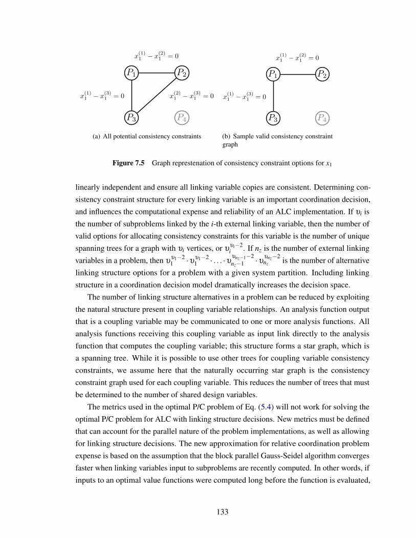
P1 P2
P3 P4
x(1)1 ! x
(2)1 = 0
x(1)1 ! x
(3)1 = 0 x
(2)1 ! x
(3)1 = 0
(a) All potential consistency constraints
P1 P2
P3 P4
x(1)1 ! x
(2)1 = 0
x(1)1 ! x
(3)1 = 0
(b) Sample valid consistency constraintgraph
Figure 7.5 Graph represtenation of consistency constraint options for x1
linearly independent and ensure all linking variable copies are consistent. Determining con-sistency constraint structure for every linking variable is an important coordination decision,and influences the computational expense and reliability of an ALC implementation. If υi isthe number of subproblems linked by the i-th external linking variable, then the number ofvalid options for allocating consistency constraints for this variable is the number of uniquespanning trees for a graph with υi vertices, or υ
υi−2i . If nz is the number of external linking
variables in a problem, then υυ1−21 ·υυ1−2
1 · . . . ·υυnz−1−2nz−1 ·υυnz−2
nz is the number of alternativelinking structure options for a problem with a given system partition. Including linkingstructure in a coordination decision model dramatically increases the decision space.
The number of linking structure alternatives in a problem can be reduced by exploitingthe natural structure present in coupling variable relationships. An analysis function outputthat is a coupling variable may be communicated to one or more analysis functions. Allanalysis functions receiving this coupling variable as input link directly to the analysisfunction that computes the coupling variable; this structure forms a star graph, which isa spanning tree. While it is possible to use other trees for coupling variable consistencyconstraints, we assume here that the naturally occurring star graph is the consistencyconstraint graph used for each coupling variable. This reduces the number of trees that mustbe determined to the number of shared design variables.
The metrics used in the optimal P/C problem of Eq. (5.4) will not work for solving theoptimal P/C problem for ALC with linking structure decisions. New metrics must be definedthat can account for the parallel nature of the problem implementations, as well as allowingfor linking structure decisions. The new approximation for relative coordination problemexpense is based on the assumption that the block parallel Gauss-Seidel algorithm convergesfaster when linking variables input to subproblems are recently computed. In other words, ifinputs to an optimal value functions were computed long before the function is evaluated,
133
convergence is slowed. Jacobi iteration is one extreme where all input data is from theprevious iteration. Sequential Gauss-Seidel (FPI) uses the most recently available data. FPIis known to converge faster than Jacobi iteration for linear systems [21]. These arguments donot always extend to nonlinear systems, but are assumed to be a reasonable approximationto enable a priori P/C decisions based on a system’s reduced adjacency matrix.
Once a system partition is defined, the subproblem graph can be constructed thatdescribes external linking variable relationships. along with its associated adjacency matrix.A is defined to be the N×N valued adjacency matrix for the subproblem graph in Fig.7.3, where each entry indicates the dimension of the corresponding linking variable. Theestimate for coordination expense here is:
CS =N
∑i=1
N
∑j=1
ζi jAi j
The value of ζi j quantifies how many stages previous to the evaluation of Pi the linkingvariables zi j were computed. CS not only quantifies the number of linking variables inthe coordination problem, but accounts for the length of time between linking variablecalculation and use as an input. The metric ζi j is defined as follows:
ζi j =
si− s j if si > s j
ns + si− s j if si ≤ s j
where ns = max(s) is the stage depth (i.e., the number of stages in the implementation). Themetric used here for quantifying subproblem sizes is more precise than the metric presentedin Eq. (5.2) because the exact number of consistency constraints and decision variables in anALC subproblem formulation are used. The previous metric made an approximation sincelinking structure information was not available. The size of the optimization problem forsubproblem i used here is:
SSi = (nxsi +nx`i +nyi +nyIi)+(nxsci +nyi +nyi)+(nai)
The first four terms comprise the number of decision variables in subproblem i. Thenumber of external shared variables associated with subproblem i is nxsi, the number of localvariables is nx`i, the number of internal coupling variables is nyi, and the number of external
134

input coupling variables is nyIi. The next three terms express the number of consistencyconstraints in subproblem i. The number of consistency constraints for external sharedvariables is nxsci, the number of internal coupling variable consistency constraints is equal tonyi, and the number of consistency constraints for external coupling variables is equal to nyi.The last term is the number of analysis functions (nai). The maximum subproblem size foreach stage is computed, and SSmax is the average of the maximum subproblem sizes.
The optimal P/C decision problem for parallel ALC with linking structure considerationsis to simultaneously minimize CS and SSmax by selecting a system partition p, subproblemstage assignment s, and a valid consistency constraint graph for each external shared designvariable. The partition vector is defined as before. The i-th component of (s) is the stagethat subproblem i is assigned to. External coupling variable consistency constraints areallocated according to the natural structure of each coupling variable. The length of thevector s is N, which depends on p. This complication is easily handled when the optimalP/C decision problem is solved with exhaustive enumeration. Section 6.2 illustrated how tomanage this type of dependence when using an evolutionary algorithm. The linking structuredecisions also depend on p. System partition changes the set of external shared designvariables, and the subproblems associated with each external shared design variable. Aswith stage assignment, linking structure can be handled with either exhaustive enumerationor an evolutionary algorithm. A set-valued decision variable C is defined to representproblem linking structure. The cardinality of C is equal to the number of external shareddesign variables in a problem with a given partition. Each member of this set defines theconsistency constraint graph for one of the shared variables. One approach to representinga consistency constraint graph, which must be a spanning tree, is with an edge set. Forexample, the variable x1 in Fig. 7.2 is shared between P1, P2, and P3, but the constraintson x1 appear only in c12 and c13, which are the consistency constraints connecting P1 withP2 and P1 with P3, respectively. The edge set corresponding to these constraints for x1 is〈1,2〉,〈1,3〉. The optimal P/C problem is:
minp,s,C
CS, SSmax (7.9)
Specifying p, s, and C defines completely a parallel ALC partition, coordination al-gorithm, and set of subproblem formulations. The number of P/C alternatives increasesmore quickly with problem size for this approach than without linking structure decisions.Exhaustive enumeration is only practical for systems with up to four analysis functions.Alternative solution techniques, such as evolutionary algorithms, must be employed forlarger systems.
135
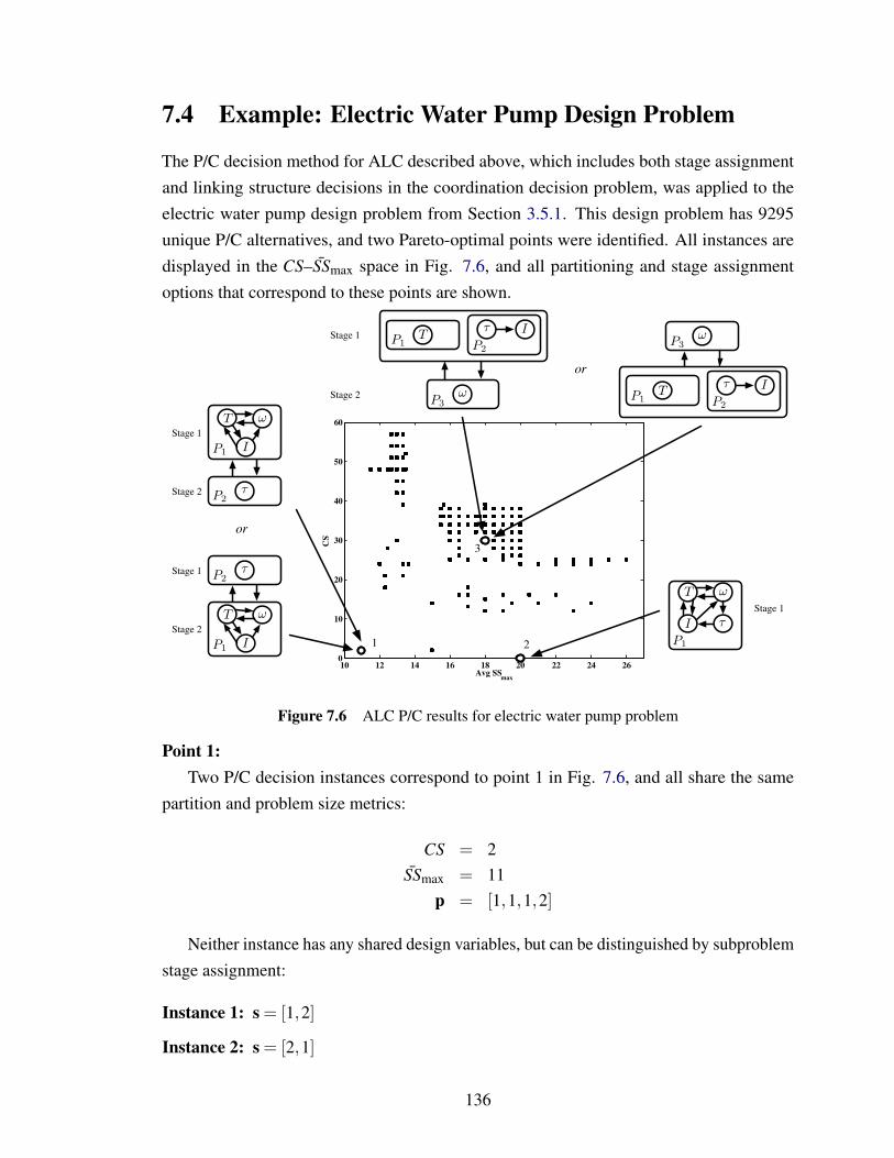
7.4 Example: Electric Water Pump Design Problem
The P/C decision method for ALC described above, which includes both stage assignmentand linking structure decisions in the coordination decision problem, was applied to theelectric water pump design problem from Section 3.5.1. This design problem has 9295unique P/C alternatives, and two Pareto-optimal points were identified. All instances aredisplayed in the CS–SSmax space in Fig. 7.6, and all partitioning and stage assignmentoptions that correspond to these points are shown.
10 12 14 16 18 20 22 24 260
10
20
30
40
50
60
Avg SSmax
CS
T !
I
!
Stage 1
Stage 2
P1
P2
T !
I
!Stage 1
Stage 2P1
P2
or
T !
I !
P1T
!
P2
I
P3
!
P3!Stage 1
Stage 2
or
P1T
!
P2
I
Stage 1
P11
3
2
Figure 7.6 ALC P/C results for electric water pump problem
Point 1:Two P/C decision instances correspond to point 1 in Fig. 7.6, and all share the same
partition and problem size metrics:
CS = 2SSmax = 11
p = [1,1,1,2]
Neither instance has any shared design variables, but can be distinguished by subproblemstage assignment:
Instance 1: s = [1,2]
Instance 2: s = [2,1]
136
Point 2:Point 2 represents the IDF formulation for the electric water pump problem, where
CS = 0 and SSmax = 20. Note that numerous P/C instances exist with larger subproblemsizes and nonzero coordination problem sizes. These points represent especially poor optionsfor constructing an ALC formulation of the electric water pump problem. Note that movingfrom point 2 to point 1 reduces SSmax from 20 to 11, and requires a coordination problemsize of just 2. This result is congruent with the analysis from Chapter 5 that indicates thisdesign problem is a good candidate for decomposition-based design optimization.
Point 3:A third point, not in the Pareto set, is examined for illustrative purposes. Point 3
corresponds to twelve unique P/C instances, all with the same partition and problem sizemetrics:
CS = 30SSmax = 18
p = [1,2,3,2]
All twelve instances have the same set of external shared design variables:
x1,x2,x3,x4,x5
The first four are shared between three subproblems, so several options exist for allocatingthe consistency constraints for these five variables. One possible set of valid consistencyconstraint graphs is shown in Fig. 7.7.
The twelve instances that correspond to point 3 are distinguished by consistency con-straint allocation and stage assignment. The two stage assignments that appear here are:
Instances 1–6: s = [1,1,2]
Instances 7–12: s = [2,2,1]
These stage assignments are illustrated in Fig. 7.6, and both specify parallel solutionof subproblems 1 and 2. No Pareto-optimal P/C instances specify parallel subproblemsolution. This is due to both problem structure and the problem size metrics selected. OnlyCS penalizes stage depth (i.e., the number of stages in a parallel implementation). Othersize metrics have been explored, such as the sum of all maximum subproblem sizes foreach stage (∑SSmax). This metric penalizes stage depth, and when employed along with CS,the resulting Pareto set contains only single-stage P/C alternatives. An ideal metric would
137
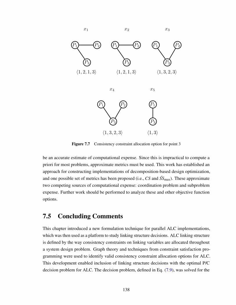
x1 x2 x3
x4
!1, 2, 1, 3" !1, 3, 2, 3"
!1, 3"
P1 P2
P3
P1 P2
P3
P1 P2
P3
P1 P2
P3
P1
P3
x5
!1, 2, 1, 3"
!1, 3, 2, 3"
Figure 7.7 Consistency constraint allocation option for point 3
be an accurate estimate of computational expense. Since this is impractical to compute apriori for most problems, approximate metrics must be used. This work has established anapproach for constructing implementations of decomposition-based design optimization,and one possible set of metrics has been proposed (i.e., CS and SSmax). These approximatetwo competing sources of computational expense: coordination problem and subproblemexpense. Further work should be performed to analyze these and other objective functionoptions.
7.5 Concluding Comments
This chapter introduced a new formulation technique for parallel ALC implementations,which was then used as a platform to study linking structure decisions. ALC linking structureis defined by the way consistency constraints on linking variables are allocated throughouta system design problem. Graph theory and techniques from constraint satisfaction pro-gramming were used to identify valid consistency constraint allocation options for ALC.This development enabled inclusion of linking structure decisions with the optimal P/Cdecision problem for ALC. The decision problem, defined in Eq. (7.9), was solved for the
138

electric water pump design problem. Opportunities for future work include an investigationof alternative problem size metrics. In the following chapter a detailed electric vehicledesign problem is developed, and the solution to the optimal P/C decision problem for theelectric vehicle problem is presented.
139
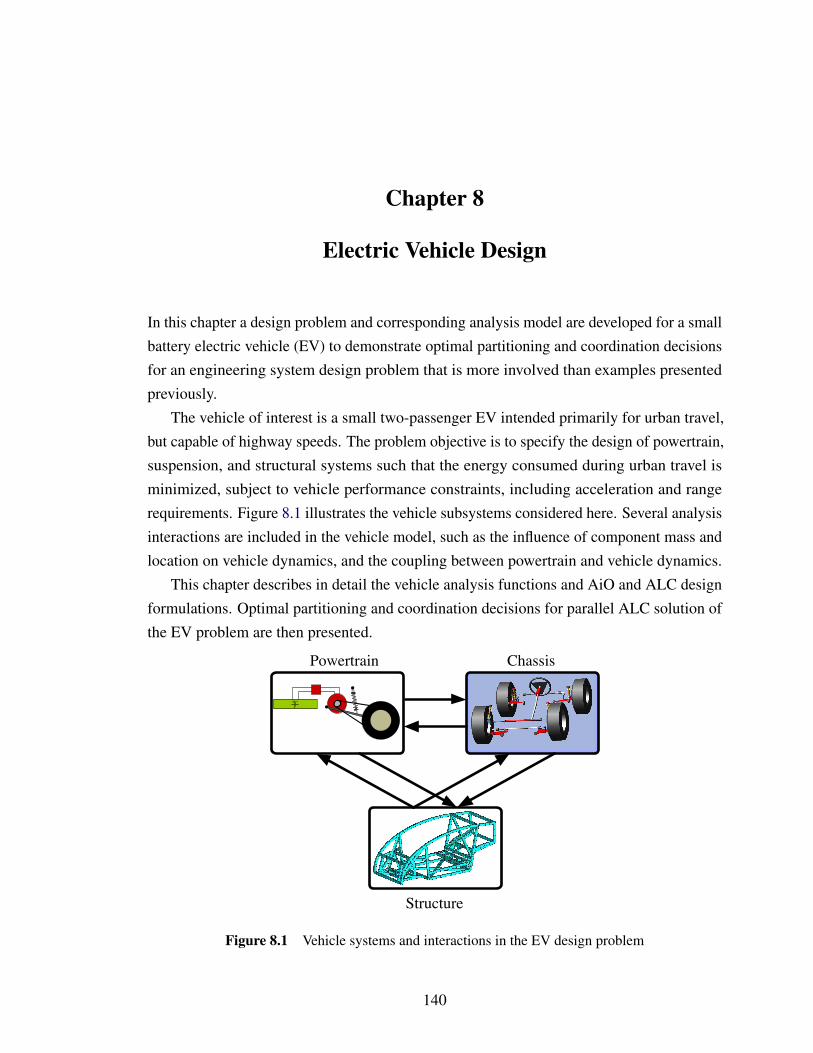
Chapter 8
Electric Vehicle Design
In this chapter a design problem and corresponding analysis model are developed for a smallbattery electric vehicle (EV) to demonstrate optimal partitioning and coordination decisionsfor an engineering system design problem that is more involved than examples presentedpreviously.
The vehicle of interest is a small two-passenger EV intended primarily for urban travel,but capable of highway speeds. The problem objective is to specify the design of powertrain,suspension, and structural systems such that the energy consumed during urban travel isminimized, subject to vehicle performance constraints, including acceleration and rangerequirements. Figure 8.1 illustrates the vehicle subsystems considered here. Several analysisinteractions are included in the vehicle model, such as the influence of component mass andlocation on vehicle dynamics, and the coupling between powertrain and vehicle dynamics.
This chapter describes in detail the vehicle analysis functions and AiO and ALC designformulations. Optimal partitioning and coordination decisions for parallel ALC solution ofthe EV problem are then presented.
ChassisPowertrain
Structure
Figure 8.1 Vehicle systems and interactions in the EV design problem
140

8.1 Vehicle Description
Battery electric vehicles use chemical energy stored in rechargeable batteries as the solepower source to provide locomotion via one or more electric motors, whereas conventionalautomobiles utilize internal combustion (IC) engines directly coupled to the vehicle drivetrain, and hybrid electric vehicles (HEVs) employ both electric motors and internal combus-tion engines. As with HEVs, EVs can recover energy during braking by using drive motor(s)as generators. This energy is lost as waste heat in conventional vehicles, but can be storedfor future use in EVs and HEVs. HEVs offer improved fuel economy over conventionalvehicles, but at increased complexity and cost. EVs are mechanically more simple thanHEVs or conventional vehicles, with very few moving parts, and provide very high levels ofenergy efficiency [33]. The primary challenge in EV design is the energy storage system;current battery technology does not enable EV range comparable to HEVs or conventionalvehicles. While EVs without some type of range extender (such as a genset trailer [58]) areimpractical for long-distance travel, they have great utility for short to medium distanceexcursions. The EV discussed in this chapter has a range of at least 100 miles (161 km),which is long enough to satisfy the needs of more than 95% of light-duty vehicle trips takenin 2001 [44]. This chapter introduces an integrated approach to EV design; simultaneousconsideration of major vehicle systems enables analysis of subsystem interactions andtradeoffs, and can aid efforts in enhancing EV performance to improve energy efficiencyand competitiveness with HEVs and conventional vehicles.
The EV under consideration here is a two-seat vehicle intended primarily for urbantravel, but capable of highway operation. Figure 8.2 shows a top view of major vehiclecomponents and dimensions. Each rear wheel is driven by an electric traction motor; asynchronous belt provides speed reduction between each motor and rear wheel. The motorsare mounted on the rear suspension trailing arms, but are located near the trailing armpivots to help minimize unsprung vehicle mass. The front suspension is a Macpherson strutconfiguration. The low rolling resistance P145/70R12 tires help reduce energy consumption.The vehicle belongs to the minicompact vehicle class, and has a track width of W = 1.27m and a wheelbase of L = 1.80 m. The lithium ion battery width (bw), length (b`), andlongitudinal position (xb) all vary in this design problem, but the battery must fit in the spaceindicated by the dashed box of width bwmax = 1.20 m and length b`max = 1.05 m. The sizeand location of the battery has profound influence over vehicle dynamics performance. Thecoordinate system used in this model is illustrated in the figure.
In recent years great emphasis has been placed on the development of HEVs, andincreasingly, EVs. These new vehicle configurations present substantial design challenges.
141
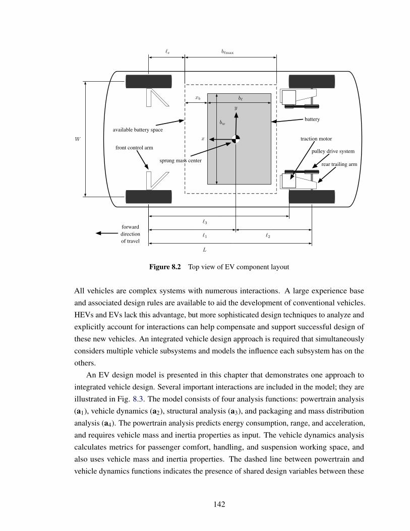
sprung mass center
battery
b!max!e
xb b!
bw
front control arm
available battery space
rear trailing arm
W
L
!1 !2
!3
pulley drive system
traction motorx
y
forward direction of travel
Figure 8.2 Top view of EV component layout
All vehicles are complex systems with numerous interactions. A large experience baseand associated design rules are available to aid the development of conventional vehicles.HEVs and EVs lack this advantage, but more sophisticated design techniques to analyze andexplicitly account for interactions can help compensate and support successful design ofthese new vehicles. An integrated vehicle design approach is required that simultaneouslyconsiders multiple vehicle subsystems and models the influence each subsystem has on theothers.
An EV design model is presented in this chapter that demonstrates one approach tointegrated vehicle design. Several important interactions are included in the model; they areillustrated in Fig. 8.3. The model consists of four analysis functions: powertrain analysis(a1), vehicle dynamics (a2), structural analysis (a3), and packaging and mass distributionanalysis (a4). The powertrain analysis predicts energy consumption, range, and acceleration,and requires vehicle mass and inertia properties as input. The vehicle dynamics analysiscalculates metrics for passenger comfort, handling, and suspension working space, andalso uses vehicle mass and inertia properties. The dashed line between powertrain andvehicle dynamics functions indicates the presence of shared design variables between these
142
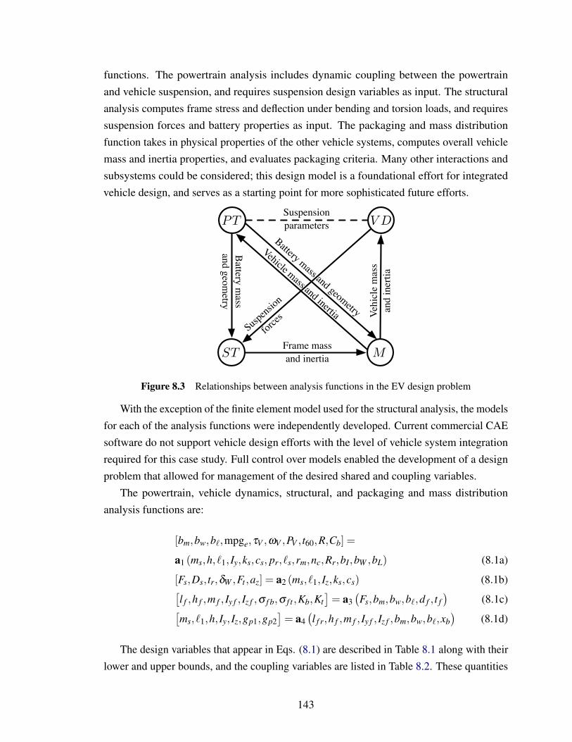
functions. The powertrain analysis includes dynamic coupling between the powertrainand vehicle suspension, and requires suspension design variables as input. The structuralanalysis computes frame stress and deflection under bending and torsion loads, and requiressuspension forces and battery properties as input. The packaging and mass distributionfunction takes in physical properties of the other vehicle systems, computes overall vehiclemass and inertia properties, and evaluates packaging criteria. Many other interactions andsubsystems could be considered; this design model is a foundational effort for integratedvehicle design, and serves as a starting point for more sophisticated future efforts.
PT
ST
V D
M
Suspensionparameters
Suspens
ion
forces
Frame mass and inertia
Vehi
cle
mas
s an
d in
ertia
Battery mass
and geometry
Vehicle mass and inertia
Battery mass and geometry
Figure 8.3 Relationships between analysis functions in the EV design problem
With the exception of the finite element model used for the structural analysis, the modelsfor each of the analysis functions were independently developed. Current commercial CAEsoftware do not support vehicle design efforts with the level of vehicle system integrationrequired for this case study. Full control over models enabled the development of a designproblem that allowed for management of the desired shared and coupling variables.
The powertrain, vehicle dynamics, structural, and packaging and mass distributionanalysis functions are:
[bm,bw,b`,mpge,τV ,ωV ,PV , t60,R,Cb] =
a1 (ms,h, `1, Iy,ks,cs, pr, `s,rm,nc,Rr,bI,bW ,bL) (8.1a)
[Fs,Ds, tr,δW ,Ft ,az] = a2 (ms, `1, Iz,ks,cs) (8.1b)[l f ,h f ,m f , Iy f , Iz f ,σ f b,σ f t ,Kb,Kt
]= a3
(Fs,bm,bw,b`,d f , t f
)(8.1c)[
ms, `1,h, Iy, Iz,gp1,gp2]= a4
(l f r,h f ,m f , Iy f , Iz f ,bm,bw,b`,xb
)(8.1d)
The design variables that appear in Eqs. (8.1) are described in Table 8.1 along with theirlower and upper bounds, and the coupling variables are listed in Table 8.2. These quantities
143
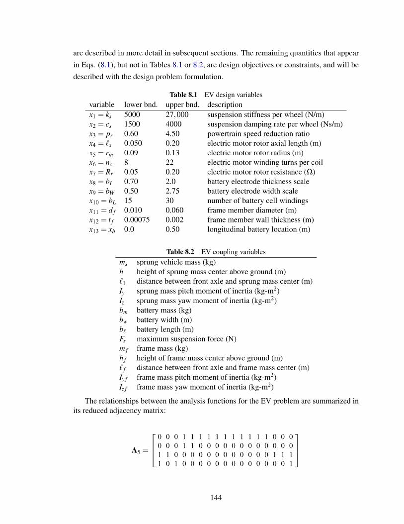
are described in more detail in subsequent sections. The remaining quantities that appearin Eqs. (8.1), but not in Tables 8.1 or 8.2, are design objectives or constraints, and will bedescribed with the design problem formulation.
Table 8.1 EV design variablesvariable lower bnd. upper bnd. descriptionx1 = ks 5000 27,000 suspension stiffness per wheel (N/m)x2 = cs 1500 4000 suspension damping rate per wheel (Ns/m)x3 = pr 0.60 4.50 powertrain speed reduction ratiox4 = `s 0.050 0.20 electric motor rotor axial length (m)x5 = rm 0.09 0.13 electric motor rotor radius (m)x6 = nc 8 22 electric motor winding turns per coilx7 = Rr 0.05 0.20 electric motor rotor resistance (Ω)x8 = bI 0.70 2.0 battery electrode thickness scalex9 = bW 0.50 2.75 battery electrode width scalex10 = bL 15 30 number of battery cell windingsx11 = d f 0.010 0.060 frame member diameter (m)x12 = t f 0.00075 0.002 frame member wall thickness (m)x13 = xb 0.0 0.50 longitudinal battery location (m)
Table 8.2 EV coupling variablesms sprung vehicle mass (kg)h height of sprung mass center above ground (m)`1 distance between front axle and sprung mass center (m)Iy sprung mass pitch moment of inertia (kg-m2)Iz sprung mass yaw moment of inertia (kg-m2)bm battery mass (kg)bw battery width (m)b` battery length (m)Fs maximum suspension force (N)m f frame mass (kg)h f height of frame mass center above ground (m)` f distance between front axle and frame mass center (m)Iy f frame mass pitch moment of inertia (kg-m2)Iz f frame mass yaw moment of inertia (kg-m2)
The relationships between the analysis functions for the EV problem are summarized inits reduced adjacency matrix:
A5 =
0 0 0 1 1 1 1 1 1 1 1 1 1 1 0 0 00 0 0 1 1 0 0 0 0 0 0 0 0 0 0 0 01 1 0 0 0 0 0 0 0 0 0 0 0 0 1 1 11 0 1 0 0 0 0 0 0 0 0 0 0 0 0 0 1
144
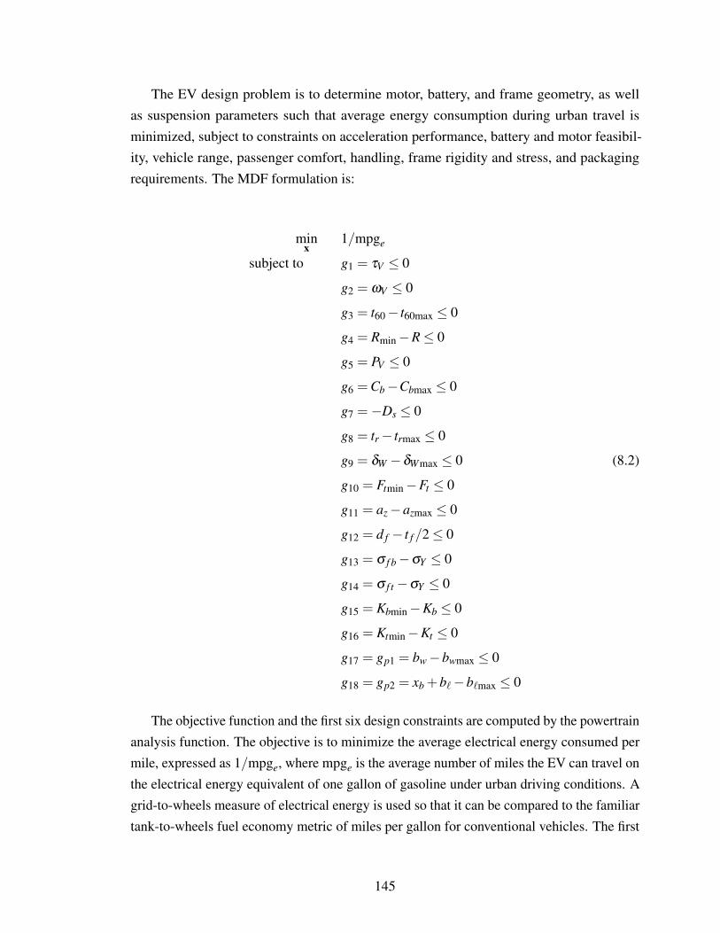
The EV design problem is to determine motor, battery, and frame geometry, as wellas suspension parameters such that average energy consumption during urban travel isminimized, subject to constraints on acceleration performance, battery and motor feasibil-ity, vehicle range, passenger comfort, handling, frame rigidity and stress, and packagingrequirements. The MDF formulation is:
minx
1/mpge
subject to g1 = τV ≤ 0
g2 = ωV ≤ 0
g3 = t60− t60max ≤ 0
g4 = Rmin−R≤ 0
g5 = PV ≤ 0
g6 = Cb−Cbmax ≤ 0
g7 =−Ds ≤ 0
g8 = tr− trmax ≤ 0
g9 = δW −δWmax ≤ 0 (8.2)
g10 = Ftmin−Ft ≤ 0
g11 = az−azmax ≤ 0
g12 = d f − t f /2≤ 0
g13 = σ f b−σY ≤ 0
g14 = σ f t−σY ≤ 0
g15 = Kbmin−Kb ≤ 0
g16 = Ktmin−Kt ≤ 0
g17 = gp1 = bw−bwmax ≤ 0
g18 = gp2 = xb +b`−b`max ≤ 0
The objective function and the first six design constraints are computed by the powertrainanalysis function. The objective is to minimize the average electrical energy consumed permile, expressed as 1/mpge, where mpge is the average number of miles the EV can travel onthe electrical energy equivalent of one gallon of gasoline under urban driving conditions. Agrid-to-wheels measure of electrical energy is used so that it can be compared to the familiartank-to-wheels fuel economy metric of miles per gallon for conventional vehicles. The first
145
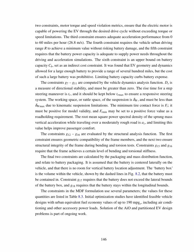
two constraints, motor torque and speed violation metrics, ensure that the electric motor iscapable of powering the EV through the desired drive cycle without exceeding torque orspeed limitations. The third constraint ensures adequate acceleration performance from 0to 60 miles per hour (26.8 m/s). The fourth constraint requires the vehicle urban drivingrange R to achieve a minimum value without risking battery damage, and the fifth constraintrequires that the battery power capacity is adequate to supply power needs throughout thedriving and acceleration simulations. The sixth constraint is an upper bound on batterycapacity Cb, set as an indirect cost constraint. It was found that EV geometry and dynamicsallowed for a large enough battery to provide a range of several hundred miles, but the costof such a large battery was prohibitive. Limiting battery capacity curbs battery expense.
The constraints g7 – g11 are computed by the vehicle dynamics analysis function. Ds isa measure of directional stability, and must be greater than zero. The rise time for a stepsteering maneuver is tr, and it should be kept below trmax to ensure a responsive steeringsystem. The working space, or rattle space, of the suspension is δW , and must be less thanδWmax due to kinematic suspension limitations. The minimum tire contact force is Ft ; itmust be positive for model validity, and Ftmin may be set to a positive force value as aroadholding requirement. The root mean square power spectral density of the sprung massvertical acceleration while traveling over a moderately rough road is az, and limiting thisvalue helps improve passenger comfort.
The constraints g12 – g16 are evaluated by the structural analysis function. The firstconstraint ensures geometric compatibility of the frame members, and the next two ensurestructural integrity of the frame during bending and torsion tests. Constraints g15 and g16
require that the frame achieves a certain level of bending and torsional stiffness.The final two constraints are calculated by the packaging and mass distribution function,
and relate to battery packaging. It is assumed that the battery is centered laterally on thevehicle, and that there is no room for vertical battery location adjustment. The ‘battery box’is the volume within the vehicle, shown by the dashed lines in Fig. 8.2, that the battery mustbe contained in. Constraint g17 requires that the battery does not exceed the lateral boundsof the battery box, and g18 requires that the battery stays within the longitudinal bounds.
The constraints in the MDF formulation use several parameters; the values for thesequantities are listed in Table 8.3. Initial optimization studies have identified feasible vehicledesigns with urban equivalent fuel economy values of up to 190 mpge, including air condi-tioning and other accessory power loads. Solution of the AiO and partitioned EV designproblems is part of ongoing work.
146
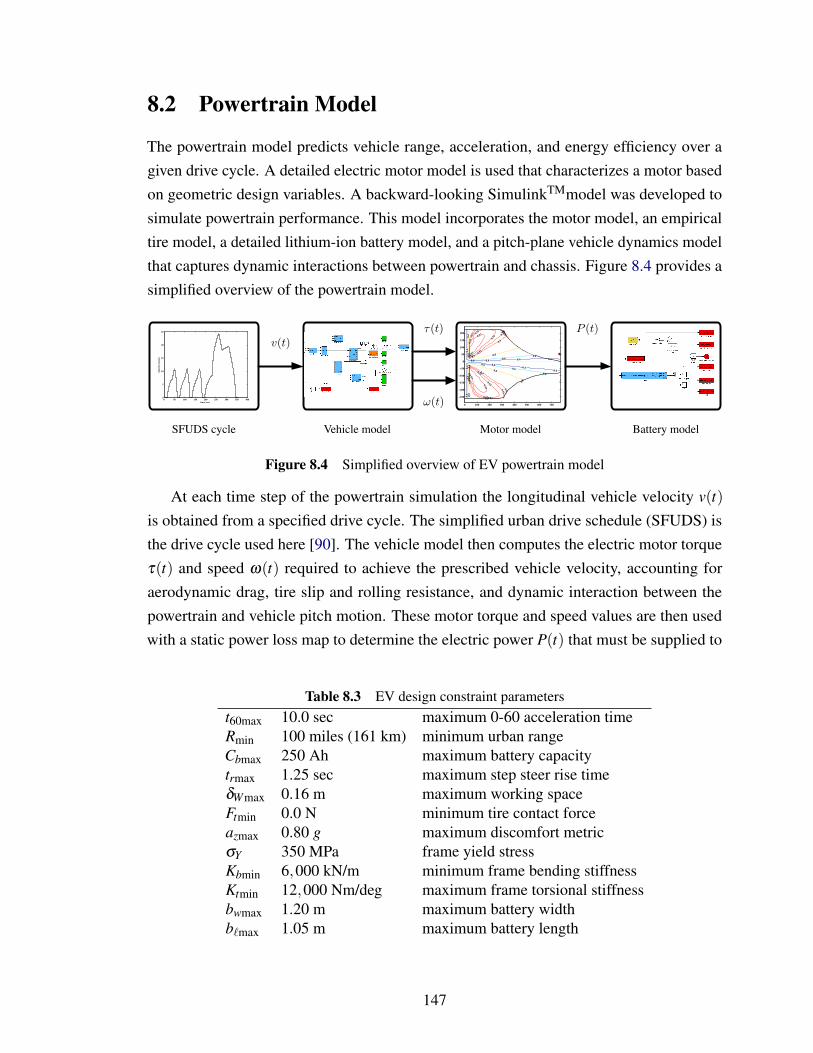
8.2 Powertrain Model
The powertrain model predicts vehicle range, acceleration, and energy efficiency over agiven drive cycle. A detailed electric motor model is used that characterizes a motor basedon geometric design variables. A backward-looking SimulinkTMmodel was developed tosimulate powertrain performance. This model incorporates the motor model, an empiricaltire model, a detailed lithium-ion battery model, and a pitch-plane vehicle dynamics modelthat captures dynamic interactions between powertrain and chassis. Figure 8.4 provides asimplified overview of the powertrain model.
0 50 100 150 200 250 300 350 4000
5
10
15
20
25
time (sec)
vel
oci
ty (
m/s
ec)
SFUDS cycle Vehicle model Motor model
0.4
0.40.4 0.4
0.4
0.4
0.4
0.4
0.4
0.4
0.6
0.60.6
0.6
0.6
0.6
0.6
0.6
0.6
0.8 0.8
0.8
0.8
0.8
0.8
0.8
0.8
0.9
0.9
0.9
0.9
0.9
0.9
0.9
0.9
0.9
0.91
0.91
0.91
0.91
0.91
0.91
0.91
0.91
0.91
0.92
0.92
0.92
0.92
0.92
0.92
0.92
0.92
0.92
0.93
0.93
0.93
0.93
0.93
0.93
0.94
0.94
0.95
0.95
0.96
0.96
0.97
0.97
0.98
0.98
0.99
0.99
1
1
1
0 100 200 300 400 500 600 700
!250
!200
!150
!100
!50
0
50
100
150
200
v(t)!(t)
!(t)
Battery model
P (t)
Figure 8.4 Simplified overview of EV powertrain model
At each time step of the powertrain simulation the longitudinal vehicle velocity v(t)is obtained from a specified drive cycle. The simplified urban drive schedule (SFUDS) isthe drive cycle used here [90]. The vehicle model then computes the electric motor torqueτ(t) and speed ω(t) required to achieve the prescribed vehicle velocity, accounting foraerodynamic drag, tire slip and rolling resistance, and dynamic interaction between thepowertrain and vehicle pitch motion. These motor torque and speed values are then usedwith a static power loss map to determine the electric power P(t) that must be supplied to
Table 8.3 EV design constraint parameterst60max 10.0 sec maximum 0-60 acceleration timeRmin 100 miles (161 km) minimum urban rangeCbmax 250 Ah maximum battery capacitytrmax 1.25 sec maximum step steer rise timeδWmax 0.16 m maximum working spaceFtmin 0.0 N minimum tire contact forceazmax 0.80 g maximum discomfort metricσY 350 MPa frame yield stressKbmin 6,000 kN/m minimum frame bending stiffnessKtmin 12,000 Nm/deg maximum frame torsional stiffnessbwmax 1.20 m maximum battery widthb`max 1.05 m maximum battery length
147
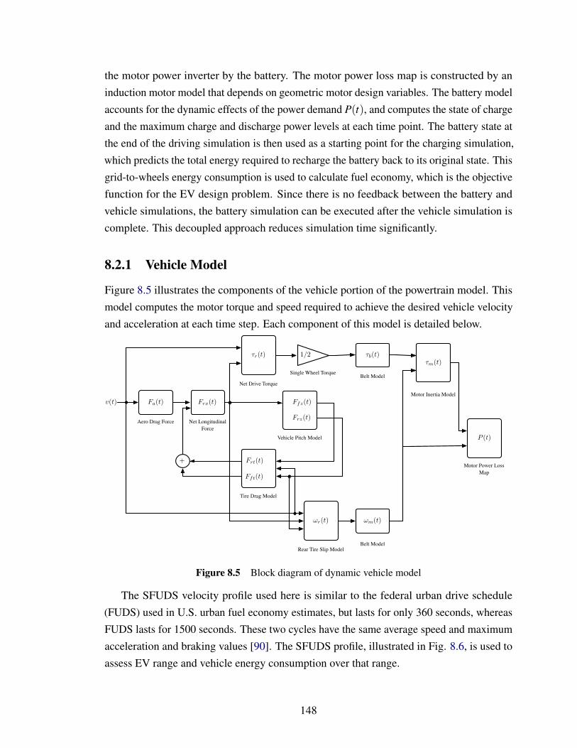
the motor power inverter by the battery. The motor power loss map is constructed by aninduction motor model that depends on geometric motor design variables. The battery modelaccounts for the dynamic effects of the power demand P(t), and computes the state of chargeand the maximum charge and discharge power levels at each time point. The battery state atthe end of the driving simulation is then used as a starting point for the charging simulation,which predicts the total energy required to recharge the battery back to its original state. Thisgrid-to-wheels energy consumption is used to calculate fuel economy, which is the objectivefunction for the EV design problem. Since there is no feedback between the battery andvehicle simulations, the battery simulation can be executed after the vehicle simulation iscomplete. This decoupled approach reduces simulation time significantly.
8.2.1 Vehicle Model
Figure 8.5 illustrates the components of the vehicle portion of the powertrain model. Thismodel computes the motor torque and speed required to achieve the desired vehicle velocityand acceleration at each time step. Each component of this model is detailed below.
v(t) Frx(t)
Net LongitudinalForce
Aero Drag Force
Fa(t)
Vehicle Pitch Model
Ffz(t)
Frz(t)
Tire Drag Model
+ Frt(t)
Fft(t)
Rear Tire Slip Model
!r(t)
Net Drive Torque
!r(t)
Belt Model
1/2
Single Wheel Torque
!m(t)
Motor Inertia Model
!b(t)
!m(t)
Belt Model
Motor Power Loss Map
P (t)
Figure 8.5 Block diagram of dynamic vehicle model
The SFUDS velocity profile used here is similar to the federal urban drive schedule(FUDS) used in U.S. urban fuel economy estimates, but lasts for only 360 seconds, whereasFUDS lasts for 1500 seconds. These two cycles have the same average speed and maximumacceleration and braking values [90]. The SFUDS profile, illustrated in Fig. 8.6, is used toassess EV range and vehicle energy consumption over that range.
148
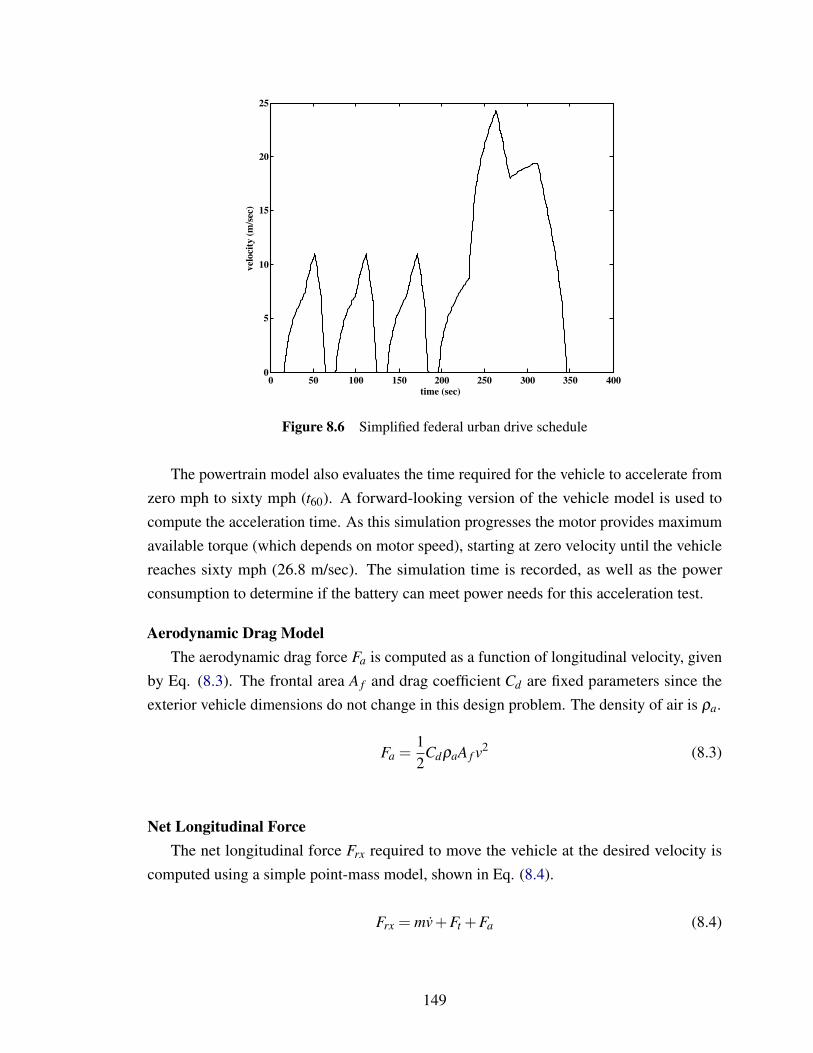
0 50 100 150 200 250 300 350 4000
5
10
15
20
25
time (sec)
velo
city
(m/se
c)
Figure 8.6 Simplified federal urban drive schedule
The powertrain model also evaluates the time required for the vehicle to accelerate fromzero mph to sixty mph (t60). A forward-looking version of the vehicle model is used tocompute the acceleration time. As this simulation progresses the motor provides maximumavailable torque (which depends on motor speed), starting at zero velocity until the vehiclereaches sixty mph (26.8 m/sec). The simulation time is recorded, as well as the powerconsumption to determine if the battery can meet power needs for this acceleration test.
Aerodynamic Drag ModelThe aerodynamic drag force Fa is computed as a function of longitudinal velocity, given
by Eq. (8.3). The frontal area A f and drag coefficient Cd are fixed parameters since theexterior vehicle dimensions do not change in this design problem. The density of air is ρa.
Fa =12
CdρaA f v2 (8.3)
Net Longitudinal ForceThe net longitudinal force Frx required to move the vehicle at the desired velocity is
computed using a simple point-mass model, shown in Eq. (8.4).
Frx = mv+Ft +Fa (8.4)
149
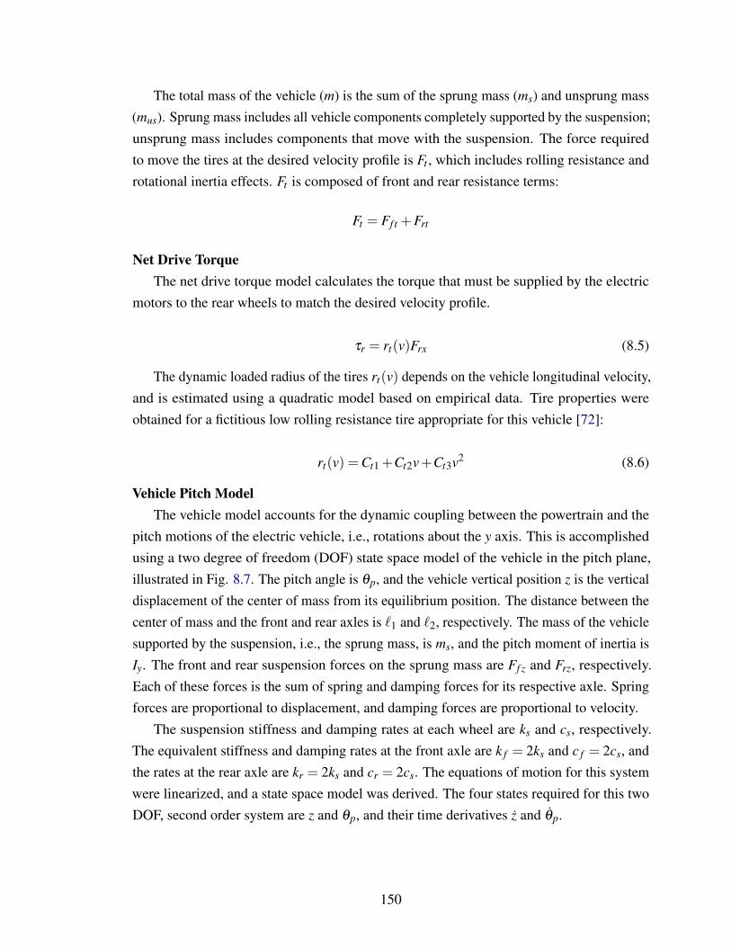
The total mass of the vehicle (m) is the sum of the sprung mass (ms) and unsprung mass(mus). Sprung mass includes all vehicle components completely supported by the suspension;unsprung mass includes components that move with the suspension. The force requiredto move the tires at the desired velocity profile is Ft , which includes rolling resistance androtational inertia effects. Ft is composed of front and rear resistance terms:
Ft = Ff t +Frt
Net Drive TorqueThe net drive torque model calculates the torque that must be supplied by the electric
motors to the rear wheels to match the desired velocity profile.
τr = rt(v)Frx (8.5)
The dynamic loaded radius of the tires rt(v) depends on the vehicle longitudinal velocity,and is estimated using a quadratic model based on empirical data. Tire properties wereobtained for a fictitious low rolling resistance tire appropriate for this vehicle [72]:
rt(v) = Ct1 +Ct2v+Ct3v2 (8.6)
Vehicle Pitch ModelThe vehicle model accounts for the dynamic coupling between the powertrain and the
pitch motions of the electric vehicle, i.e., rotations about the y axis. This is accomplishedusing a two degree of freedom (DOF) state space model of the vehicle in the pitch plane,illustrated in Fig. 8.7. The pitch angle is θp, and the vehicle vertical position z is the verticaldisplacement of the center of mass from its equilibrium position. The distance between thecenter of mass and the front and rear axles is `1 and `2, respectively. The mass of the vehiclesupported by the suspension, i.e., the sprung mass, is ms, and the pitch moment of inertia isIy. The front and rear suspension forces on the sprung mass are Ff z and Frz, respectively.Each of these forces is the sum of spring and damping forces for its respective axle. Springforces are proportional to displacement, and damping forces are proportional to velocity.
The suspension stiffness and damping rates at each wheel are ks and cs, respectively.The equivalent stiffness and damping rates at the front axle are k f = 2ks and c f = 2cs, andthe rates at the rear axle are kr = 2ks and cr = 2cs. The equations of motion for this systemwere linearized, and a state space model was derived. The four states required for this twoDOF, second order system are z and θp, and their time derivatives z and θp.
150
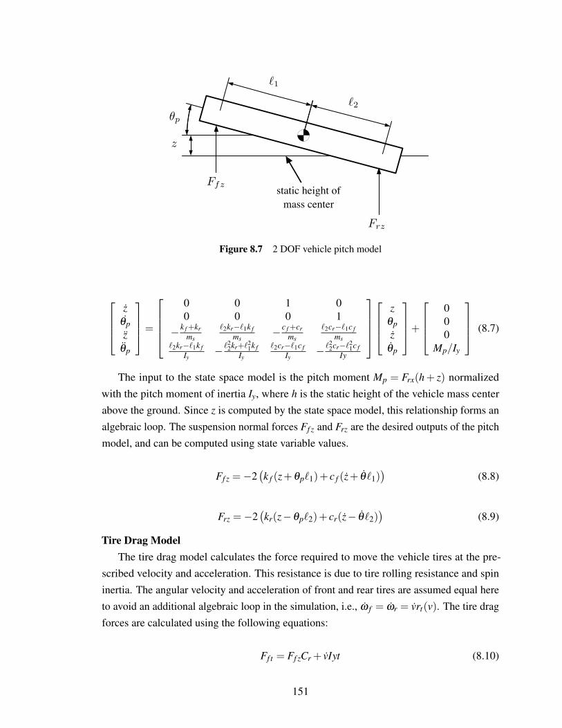
Frz
Ffz
!p
z
!1
!2
static height of mass center
Figure 8.7 2 DOF vehicle pitch model
z
θpz
θp
=
0 0 1 00 0 0 1
−k f +krms
`2kr−`1k fms
−c f +crms
`2cr−`1c fms
`2kr−`1k fIy
− `22kr+`2
1k fIy
`2cr−`1c fIy
− `22cr−`2
1c fIy
zθpz
θp
+
000
Mp/Iy
(8.7)
The input to the state space model is the pitch moment Mp = Frx(h + z) normalizedwith the pitch moment of inertia Iy, where h is the static height of the vehicle mass centerabove the ground. Since z is computed by the state space model, this relationship forms analgebraic loop. The suspension normal forces Ff z and Frz are the desired outputs of the pitchmodel, and can be computed using state variable values.
Ff z =−2(k f (z+θp`1)+ c f (z+ θ`1)
)(8.8)
Frz =−2(kr(z−θp`2)+ cr(z− θ`2)
)(8.9)
Tire Drag ModelThe tire drag model calculates the force required to move the vehicle tires at the pre-
scribed velocity and acceleration. This resistance is due to tire rolling resistance and spininertia. The angular velocity and acceleration of front and rear tires are assumed equal hereto avoid an additional algebraic loop in the simulation, i.e., ω f = ωr = vrt(v). The tire dragforces are calculated using the following equations:
Ff t = Ff zCr + vIyt (8.10)
151
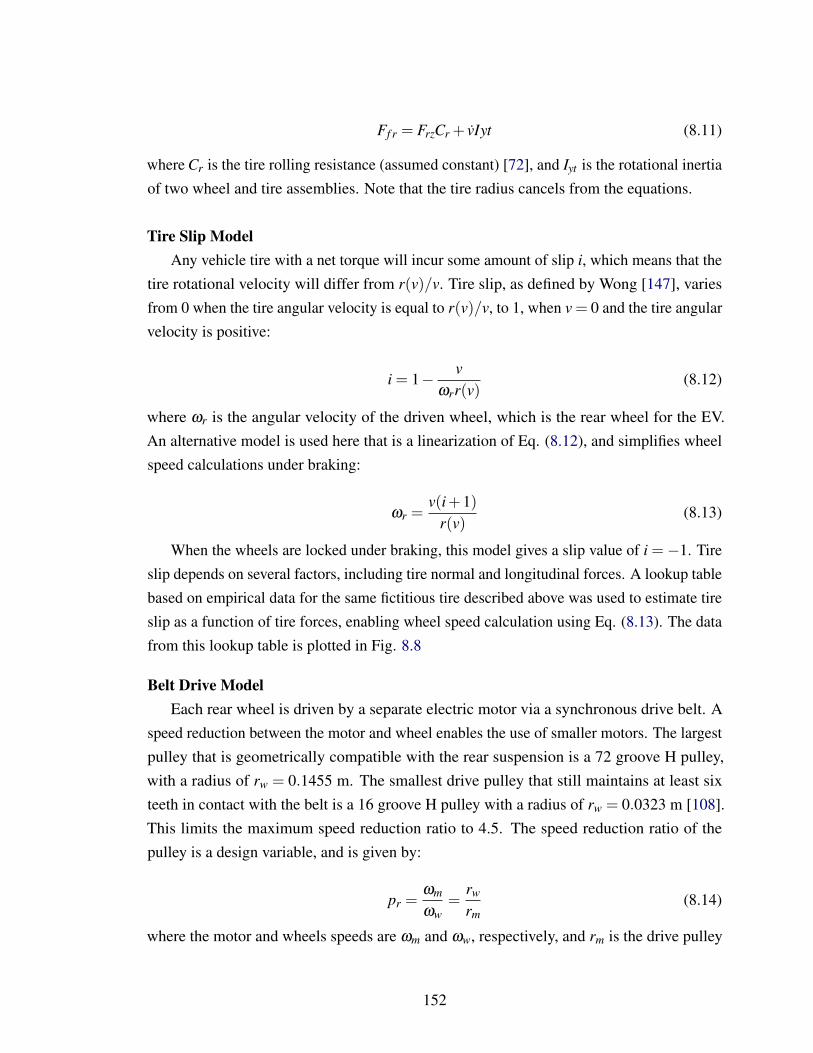
Ff r = FrzCr + vIyt (8.11)
where Cr is the tire rolling resistance (assumed constant) [72], and Iyt is the rotational inertiaof two wheel and tire assemblies. Note that the tire radius cancels from the equations.
Tire Slip ModelAny vehicle tire with a net torque will incur some amount of slip i, which means that the
tire rotational velocity will differ from r(v)/v. Tire slip, as defined by Wong [147], variesfrom 0 when the tire angular velocity is equal to r(v)/v, to 1, when v = 0 and the tire angularvelocity is positive:
i = 1− vωrr(v)
(8.12)
where ωr is the angular velocity of the driven wheel, which is the rear wheel for the EV.An alternative model is used here that is a linearization of Eq. (8.12), and simplifies wheelspeed calculations under braking:
ωr =v(i+1)
r(v)(8.13)
When the wheels are locked under braking, this model gives a slip value of i =−1. Tireslip depends on several factors, including tire normal and longitudinal forces. A lookup tablebased on empirical data for the same fictitious tire described above was used to estimate tireslip as a function of tire forces, enabling wheel speed calculation using Eq. (8.13). The datafrom this lookup table is plotted in Fig. 8.8
Belt Drive ModelEach rear wheel is driven by a separate electric motor via a synchronous drive belt. A
speed reduction between the motor and wheel enables the use of smaller motors. The largestpulley that is geometrically compatible with the rear suspension is a 72 groove H pulley,with a radius of rw = 0.1455 m. The smallest drive pulley that still maintains at least sixteeth in contact with the belt is a 16 groove H pulley with a radius of rw = 0.0323 m [108].This limits the maximum speed reduction ratio to 4.5. The speed reduction ratio of thepulley is a design variable, and is given by:
pr =ωm
ωw=
rw
rm(8.14)
where the motor and wheels speeds are ωm and ωw, respectively, and rm is the drive pulley
152
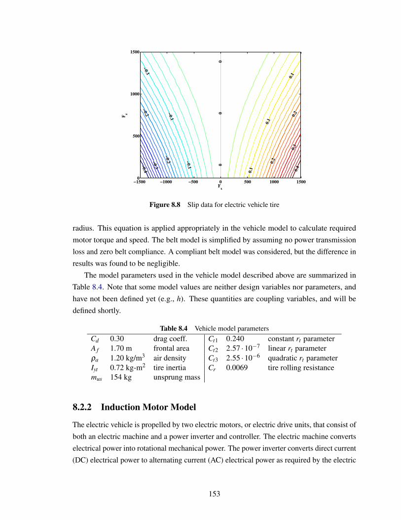
−0.4
−0.3
−0.2
−0.2
−0.1
−0.1
−0.1
00
0
0.1
0.1
0.1
0.2
0.20.3
0.4
Fx
F z
−1500 −1000 −500 0 500 1000 15000
500
1000
1500
Figure 8.8 Slip data for electric vehicle tire
radius. This equation is applied appropriately in the vehicle model to calculate requiredmotor torque and speed. The belt model is simplified by assuming no power transmissionloss and zero belt compliance. A compliant belt model was considered, but the difference inresults was found to be negligible.
The model parameters used in the vehicle model described above are summarized inTable 8.4. Note that some model values are neither design variables nor parameters, andhave not been defined yet (e.g., h). These quantities are coupling variables, and will bedefined shortly.
Table 8.4 Vehicle model parametersCd 0.30 drag coeff. Ct1 0.240 constant rt parameterA f 1.70 m frontal area Ct2 2.57 ·10−7 linear rt parameterρa 1.20 kg/m3 air density Ct3 2.55 ·10−6 quadratic rt parameterIyt 0.72 kg-m2 tire inertia Cr 0.0069 tire rolling resistancemus 154 kg unsprung mass
8.2.2 Induction Motor Model
The electric vehicle is propelled by two electric motors, or electric drive units, that consist ofboth an electric machine and a power inverter and controller. The electric machine convertselectrical power into rotational mechanical power. The power inverter converts direct current(DC) electrical power to alternating current (AC) electrical power as required by the electric
153
machine. The rotor of an electric machine is connected to the output shaft, and is encasedby a cylindrical stator.
Two types of motors are in popular use for electric and hybrid electric vehicles: perma-nent magnet brushless direct current (BLDC) motors, and AC induction motors (IMs). Eachtype employs a stator that produces a rotating magnetic field that interacts with the rotor’smagnetic field, causing the rotor to spin. The stator typically is wound with three phases,and is supplied with three-phase AC power. The rotor in a BLDC machine is constructedof permanent magnet material, providing a continuous magnetic field. In contrast, an IMrotor is constructed with a stack of iron sheets, with conducting bars running through therotor parallel to the output shaft. Conductive end rings electrically short these conductingbars. When the rotor is subjected to the stator’s rotating magnetic field, electric currents areinduced in the conducting bars, creating a rotating magnetic field of their own. A simplifieddiagram of an IM is shown in Fig. 8.9. BLDC motors are characteristically more efficientthan IMs, but are more expensive due to permanent magnet material. A three-phase IM waschosen as the electric drive unit for the EV. A detailed model was developed that constructsthe motor power loss map based on geometric motor design variables.
rotor
stator
output shaft
Figure 8.9 Diagram of an induction motor
Equivalent CircuitThe dynamic electrical behavior of an IM can be modeled using a equivalent circuit [24].
After several simplifications, the resulting equivalent circuit for a single phase of the IMconsists of three inductance elements and two resistance elements, one of which is variable(Fig. 8.10). The mutual inductance between the rotor and stator is Lm; the stator windingresistance is Rs; the stator and rotor leakage inductances are Lls and Llr, respectively, andthe electrical resistance through the rotor conductors is Rr. The AC power source has a rootmean square voltage (RMS) of Vs.
The rotor conductors do not have a direct electrical connection to the stator, but rather
154

Vs Lm
Rs Lls Llr
Rr/s
Figure 8.10 Equivalent circuit of an induction motor
have an indirect influence through electromagnetic interaction. The stator and rotor arecoupled in a manner similar to the primary and secondary windings of a transformer. Aswith transformers, we can include the secondary windings in a single equivalent circuit iftheir properties are viewed in the reference frame of the primary circuit. In the IM equivalentcircuit we do this by dividing the rotor resistance by the slip between the stator and rotormagnetic fields. The stator power supply frequency ωe determines the speed at which thestator magnetic field rotates, and the rotor magnetic field rotation lags the stator field if thereis any load on the motor. This lag is quantified by slip s, defined as:
s =ωe−ωr
ωe(8.15)
where ωr is the rotor electrical speed. The slip depends on supply voltage and frequency,motor construction, and load. Slip, or misalignment between the magnetic fields, gives riseto torque. If slip is zero, the magnetic fields are aligned, and no torque can be produced.At zero slip the motor is at synchronous speed, and as torque is applied slip increasesmonotonically until the breakdown torque Tem is reached. When s = 1 the motor is stalled,i.e., the rotor is stationary with the stator magnetic field rotating.
Motor Property CalculationThe dynamic motor model requires knowledge of several values that characterize an
induction motor, such as the rotor inertia, frictional losses, inductance, electrical resistanceof stator windings, and the maximum stator current. These values may be approximatedusing simple formulae. The estimated rotor mass is:
mr = πr2m`sρ f e (8.16)
where rm is the rotor radius, `s is the rotor stack length, and ρ f e is the density of iron. These
155
and other parameter values used in the induction motor model are summarized in Table 8.5.The rotational inertia of the rotor is approximately:
Jr =mrr2
m2
(8.17)
A viscous friction model is used to approximate the parasitic torque on the motor fromresistance in the bearings:
τloss(Jr) = ωmcm (8.18)
where ωm is the rotational speed of the motor output shaft in radians per second, and cm isthe viscous friction coefficient. A strong correlation was observed between Jr and cm, andan exponential model was fit to empirical motor data:
cm = Cm1
(1− Cm2
eCm3Jr
)+Cm4Jr (8.19)
The model parameters for this and other equations in this section are defined in Table 8.5.The mutual inductance is calculated from motor geometry using a model due to Amin [11].The number of stator slots (Ns) and stator windings per phase (W1) must first be calculated:
Ns = 2p1qm1 (8.20)
W1 = 2p1qnc (8.21)
where p1 is the number of pole pairs in the stator (i.e., the number of poles p divided by 2),q is the number of stator slots per phase per pole, m1 is the number of phases, and nc is thenumber of turns per coil. The mutual inductance is:
Lm =6µ0W 2
1 rm`s
π p21δg
(8.22)
where the effective air gap δg, adjusting for geometry and slot effects, is given by:
δg = 0.06rm− .0025 (8.23)
The stator leakage inductance (Lls) was observed to have a correlation with motoraspect ratio (`s/rm) and mutual inductance in empirical data for several IMs. The following
156
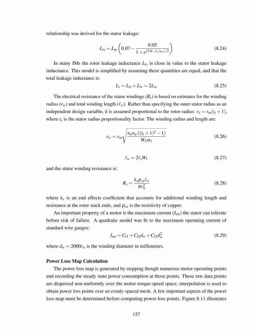
relationship was derived for the stator leakage:
Lls = Lm
(0.07− 0.05
1+ e(5.0−`s/rm)/2
)(8.24)
In many IMs the rotor leakage inductance Llr is close in value to the stator leakageinductance. This model is simplified by assuming these quantities are equal, and that thetotal leakage inductance is:
Ll = Lls +Llr = 2Lls (8.25)
The electrical resistance of the stator windings (Rs) is based on estimates for the windingradius (rw) and total winding length (`w). Rather than specifying the outer stator radius as anindependent design variable, it is assumed proportional to the rotor radius: rs = rm(ts +1),where ts is the stator radius proportionality factor. The winding radius and length are:
rw = rm
√nanp ((ts +1)2−1)
W1m1(8.26)
`w = 2`sW1 (8.27)
and the stator winding resistance is:
Rs =keρcu`w
πr2w
(8.28)
where ke is an end effects coefficient that accounts for additional winding length andresistance at the rotor stack ends, and ρcu is the resistivity of copper.
An important property of a motor is the maximum current (Ism) the stator can toleratebefore risk of failure. A quadratic model was fit to the maximum operating current ofstandard wire gauges:
Ism = CI1 +CI2dw +CI3d2w (8.29)
where dw = 2000rw is the winding diameter in millimeters.
Power Loss Map CalculationThe power loss map is generated by stepping though numerous motor operating points
and recording the steady state power consumption at those points. These raw data pointsare dispersed non-uniformly over the motor torque-speed space; interpolation is used toobtain power loss points over an evenly-spaced mesh. A few important aspects of the powerloss map must be determined before computing power loss points. Figure 8.11 illustrates
157
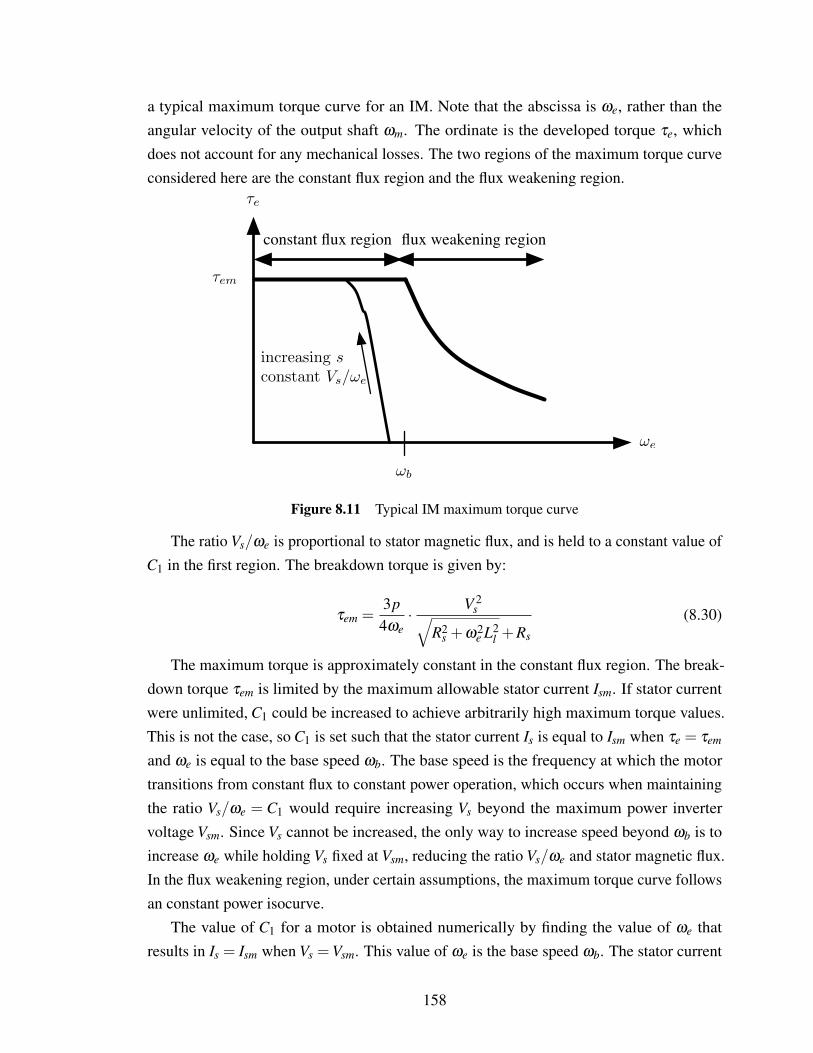
a typical maximum torque curve for an IM. Note that the abscissa is ωe, rather than theangular velocity of the output shaft ωm. The ordinate is the developed torque τe, whichdoes not account for any mechanical losses. The two regions of the maximum torque curveconsidered here are the constant flux region and the flux weakening region.
increasing sconstant Vs/!e
!e
!b
constant flux region flux weakening region
!em
!e
Figure 8.11 Typical IM maximum torque curve
The ratio Vs/ωe is proportional to stator magnetic flux, and is held to a constant value ofC1 in the first region. The breakdown torque is given by:
τem =3p4ωe· V 2
s√R2
s +ω2e L2
l +Rs
(8.30)
The maximum torque is approximately constant in the constant flux region. The break-down torque τem is limited by the maximum allowable stator current Ism. If stator currentwere unlimited, C1 could be increased to achieve arbitrarily high maximum torque values.This is not the case, so C1 is set such that the stator current Is is equal to Ism when τe = τem
and ωe is equal to the base speed ωb. The base speed is the frequency at which the motortransitions from constant flux to constant power operation, which occurs when maintainingthe ratio Vs/ωe = C1 would require increasing Vs beyond the maximum power invertervoltage Vsm. Since Vs cannot be increased, the only way to increase speed beyond ωb is toincrease ωe while holding Vs fixed at Vsm, reducing the ratio Vs/ωe and stator magnetic flux.In the flux weakening region, under certain assumptions, the maximum torque curve followsan constant power isocurve.
The value of C1 for a motor is obtained numerically by finding the value of ωe thatresults in Is = Ism when Vs = Vsm. This value of ωe is the base speed ωb. The stator current
158
for a given ωe at Vsm can be found through analysis of the equivalent circuit in Fig. 8.10.The impedance of Lm is:
Z1 = jLmωe (8.31)
where j is the imaginary number√−1. The impedance of Rs, Lls, Llr, and Rr/s in series is:
Z2 = (Rs +Rr/sm)+ jωe(Lls +Llr) (8.32)
The slip at torque breakdown sm is used in evaluating Z2 when computing the maximumstator current:
sm =Rr√
R2s +ω2
e L2l
(8.33)
Other values of slip may be used in Eq. (8.32) when calculating stator current foroperating points below maximum torque. The total circuit impedance is:
ZT =Z1Z2
Z1 +Z2(8.34)
and at maximum power inverter voltage the stator current is:
Ism =Vsm
|ZT |(8.35)
Now that ωb is known, the base speed can be calculated in terms of rotor electricalfrequency and output shaft rotational speed. First, Eq. (8.33) is used to calculate motor slipat ωb and max torque (smb). The base rotor electrical frequency is:
ωrb = ωb(1− smb) (8.36)
and the base output shaft speed is:
ωmb = 2ωrb/p (8.37)
The maximum torque in the constant flux region is almost constant torque, but notexactly due to stator effects. A small voltage adjustment is used to compensate for this:
Vs =ωe(Vsm−V0)
ωb+V0 (8.38)
where V0 is a voltage compensation parameter chosen such that the maximum torque in theconstant flux region is as close to constant as possible. Four different operating regimes areconsidered in the power loss map calculation:
159
1. Forward motoring, constant flux: ωm > 0, s > 0, and Vs/ωe constant2. Forward motoring, flux weakening: ωm > 0, s > 0, Vs constant, and ωe > ωb3. Forward regeneration, constant flux: ωm > 0, s < 0, and Vs/ωe constant4. Forward regeneration, flux weakening: ωm > 0, s < 0, Vs constant, and ωe > ωb
In the regenerative regimes the stator electrical frequency lags the rotor electrical fre-quency, resulting in negative slip, causing the motor to perform as a generator. Duringregeneration the vehicle is slowed and the motor converts mechanical kinetic energy intoelectrical energy, which may be stored for later use. The power loss map is different inthe forward motoring and regeneration regimes for two primary reasons: frictional lossesand stator resistance. Power loss values for the forward motoring, constant flux regime areobtained by stepping through ωe values from just above zero through ωb. At each value forωe the value of Vs is found using Eq. (8.38), and breakdown torque and output shaft speed isrecorded. At each speed point we step through slip values from just above zero to sm, whichis found using Eq. (8.33). At each ωe and s point, we evaluate the developed torque:
τe =3pRr
2sωe· V 2
s
(Rs +Rr/s)2 +ω2e L2
l(8.39)
The output shaft speed is recorded for each of these points, and the net output torque isfound:
τnet = τe−ωmcm (8.40)
where cm is evaluated using Eq. (8.19). The net mechanical output power is Pout = τnetωm,and can be used to evaluate motor efficiency at that operating point. The stator currentis evaluated using Eqs. (8.31) – (8.35), where Vsm and sm are replaced with Vs and s,respectively. The electrical input power to the motor is:
Pin = m1IsVs cos(∠ZT ) (8.41)
where ∠ZT is the angle between the imaginary and real parts of ZT . The power factor iscos(∠ZT ), and accounts for the influence of inductive elements on power consumption. Inthe forward regeneration, constant flux regime, the same values of ωe are used, but slipis varied from just below zero to slip at breakdown speed (which is negative). Equation(8.39) is used again to evaluate developed torque at each point. Frictional losses increase themagnitude of net torque in this case since τe < 0. Electrical output power calculations areperformed using the same equations as for forward motoring, but Pin < 0, indicating poweroutput. The breakdown torque during regeneration is slightly different than for the forward
160
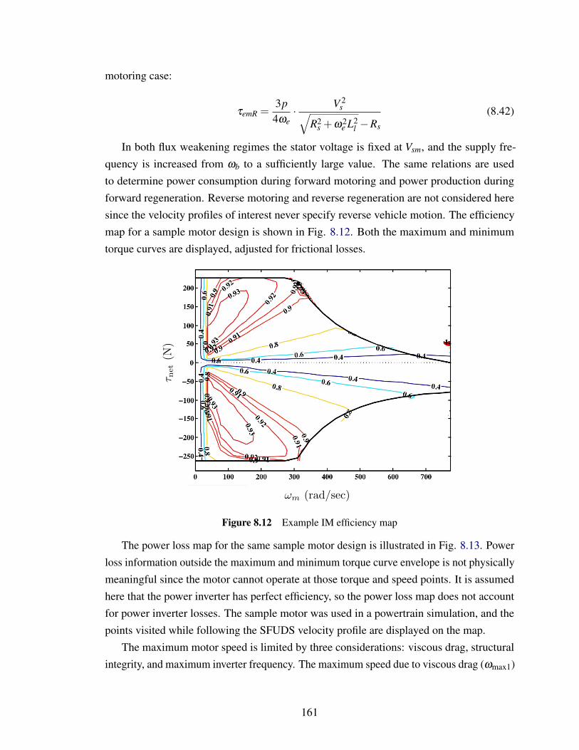
motoring case:
τemR =3p4ωe· V 2
s√R2
s +ω2e L2
l −Rs
(8.42)
In both flux weakening regimes the stator voltage is fixed at Vsm, and the supply fre-quency is increased from ωb to a sufficiently large value. The same relations are usedto determine power consumption during forward motoring and power production duringforward regeneration. Reverse motoring and reverse regeneration are not considered heresince the velocity profiles of interest never specify reverse vehicle motion. The efficiencymap for a sample motor design is shown in Fig. 8.12. Both the maximum and minimumtorque curves are displayed, adjusted for frictional losses.
!m (rad/sec)
!net
(N)
Figure 8.12 Example IM efficiency map
The power loss map for the same sample motor design is illustrated in Fig. 8.13. Powerloss information outside the maximum and minimum torque curve envelope is not physicallymeaningful since the motor cannot operate at those torque and speed points. It is assumedhere that the power inverter has perfect efficiency, so the power loss map does not accountfor power inverter losses. The sample motor was used in a powertrain simulation, and thepoints visited while following the SFUDS velocity profile are displayed on the map.
The maximum motor speed is limited by three considerations: viscous drag, structuralintegrity, and maximum inverter frequency. The maximum speed due to viscous drag (ωmax1)
161
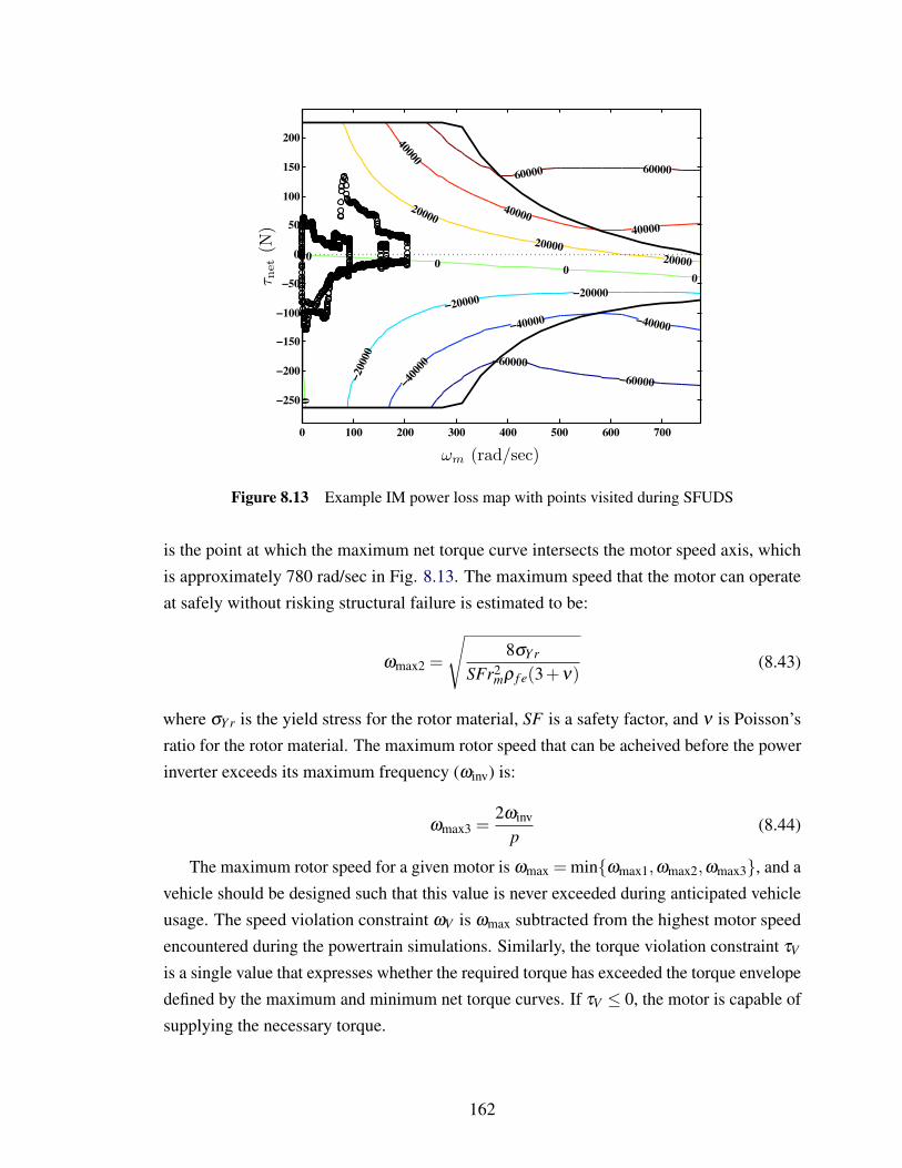
!m (rad/sec)
!net
(N)
!60000
!60000!40
000
!40000 !40000
!20
000
!20000!20000
00
00
00
20000
2000020000
40000
40000
40000
60000 60000
Torque/Speed Points Visited
0 100 200 300 400 500 600 700
!250
!200
!150
!100
!50
0
50
100
150
200
Figure 8.13 Example IM power loss map with points visited during SFUDS
is the point at which the maximum net torque curve intersects the motor speed axis, whichis approximately 780 rad/sec in Fig. 8.13. The maximum speed that the motor can operateat safely without risking structural failure is estimated to be:
ωmax2 =
√8σY r
SFr2mρ f e(3+ν)
(8.43)
where σY r is the yield stress for the rotor material, SF is a safety factor, and ν is Poisson’sratio for the rotor material. The maximum rotor speed that can be acheived before the powerinverter exceeds its maximum frequency (ωinv) is:
ωmax3 =2ωinv
p(8.44)
The maximum rotor speed for a given motor is ωmax = minωmax1,ωmax2,ωmax3, and avehicle should be designed such that this value is never exceeded during anticipated vehicleusage. The speed violation constraint ωV is ωmax subtracted from the highest motor speedencountered during the powertrain simulations. Similarly, the torque violation constraint τV
is a single value that expresses whether the required torque has exceeded the torque envelopedefined by the maximum and minimum net torque curves. If τV ≤ 0, the motor is capable ofsupplying the necessary torque.
162
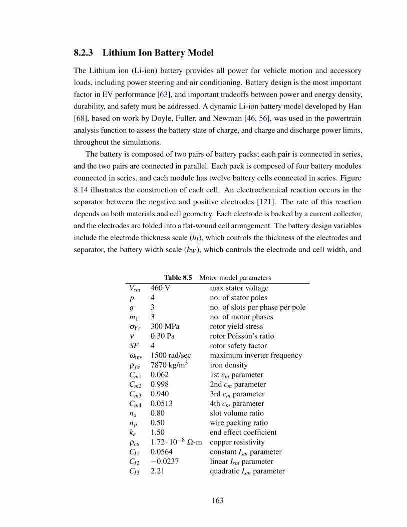
8.2.3 Lithium Ion Battery Model
The Lithium ion (Li-ion) battery provides all power for vehicle motion and accessoryloads, including power steering and air conditioning. Battery design is the most importantfactor in EV performance [63], and important tradeoffs between power and energy density,durability, and safety must be addressed. A dynamic Li-ion battery model developed by Han[68], based on work by Doyle, Fuller, and Newman [46, 56], was used in the powertrainanalysis function to assess the battery state of charge, and charge and discharge power limits,throughout the simulations.
The battery is composed of two pairs of battery packs; each pair is connected in series,and the two pairs are connected in parallel. Each pack is composed of four battery modulesconnected in series, and each module has twelve battery cells connected in series. Figure8.14 illustrates the construction of each cell. An electrochemical reaction occurs in theseparator between the negative and positive electrodes [121]. The rate of this reactiondepends on both materials and cell geometry. Each electrode is backed by a current collector,and the electrodes are folded into a flat-wound cell arrangement. The battery design variablesinclude the electrode thickness scale (bI), which controls the thickness of the electrodes andseparator, the battery width scale (bW ), which controls the electrode and cell width, and
Table 8.5 Motor model parametersVsm 460 V max stator voltagep 4 no. of stator polesq 3 no. of slots per phase per polem1 3 no. of motor phasesσY r 300 MPa rotor yield stressν 0.30 Pa rotor Poisson’s ratioSF 4 rotor safety factorωinv 1500 rad/sec maximum inverter frequencyρ f e 7870 kg/m3 iron densityCm1 0.062 1st cm parameterCm2 0.998 2nd cm parameterCm3 0.940 3rd cm parameterCm4 0.0513 4th cm parameterna 0.80 slot volume rationp 0.50 wire packing ratioke 1.50 end effect coefficientρcu 1.72 ·10−8 Ω-m copper resistivityCI1 0.0564 constant Ism parameterCI2 −0.0237 linear Ism parameterCI3 2.21 quadratic Ism parameter
163
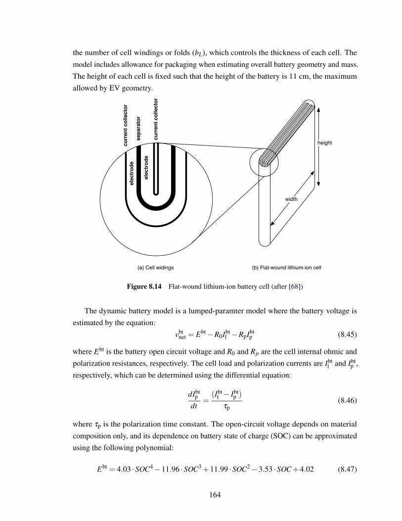
the number of cell windings or folds (bL), which controls the thickness of each cell. Themodel includes allowance for packaging when estimating overall battery geometry and mass.The height of each cell is fixed such that the height of the battery is 11 cm, the maximumallowed by EV geometry.
(a) cell winding
cu
rre
nt
co
lle
cto
r
ele
ctr
od
e
ele
ctr
od
e
cu
rre
nt
co
lle
cto
r
se
pa
rato
r
(a) Cell widings (b) Flat-wound lithium-ion cell
width
height
Figure 8.14 Flat-wound lithium-ion battery cell (after [68])
The dynamic battery model is a lumped-paramter model where the battery voltage isestimated by the equation:
vbtnet = Ebt−R0Ibt
l −RpIbtp (8.45)
where Ebt is the battery open circuit voltage and R0 and Rp are the cell internal ohmic andpolarization resistances, respectively. The cell load and polarization currents are Ibt
l and Ibtp ,
respectively, which can be determined using the differential equation:
dIbtp
dt=
(Ibtl − Ibt
p )τp
(8.46)
where τp is the polarization time constant. The open-circuit voltage depends on materialcomposition only, and its dependence on battery state of charge (SOC) can be approximatedusing the following polynomial:
Ebt = 4.03 ·SOC4−11.96 ·SOC3 +11.99 ·SOC2−3.53 ·SOC +4.02 (8.47)
164
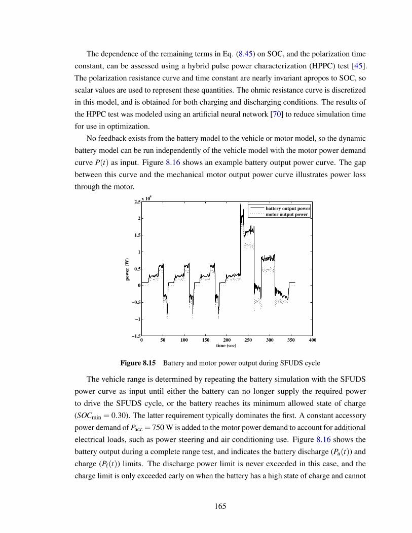
The dependence of the remaining terms in Eq. (8.45) on SOC, and the polarization timeconstant, can be assessed using a hybrid pulse power characterization (HPPC) test [45].The polarization resistance curve and time constant are nearly invariant apropos to SOC, soscalar values are used to represent these quantities. The ohmic resistance curve is discretizedin this model, and is obtained for both charging and discharging conditions. The results ofthe HPPC test was modeled using an artificial neural network [70] to reduce simulation timefor use in optimization.
No feedback exists from the battery model to the vehicle or motor model, so the dynamicbattery model can be run independently of the vehicle model with the motor power demandcurve P(t) as input. Figure 8.16 shows an example battery output power curve. The gapbetween this curve and the mechanical motor output power curve illustrates power lossthrough the motor.
0 50 100 150 200 250 300 350 400−1.5
−1
−0.5
0
0.5
1
1.5
2
2.5 x 10⁴
time (sec)
pow
er (W
)
battery output powermotor output power
Figure 8.15 Battery and motor power output during SFUDS cycle
The vehicle range is determined by repeating the battery simulation with the SFUDSpower curve as input until either the battery can no longer supply the required powerto drive the SFUDS cycle, or the battery reaches its minimum allowed state of charge(SOCmin = 0.30). The latter requirement typically dominates the first. A constant accessorypower demand of Pacc = 750 W is added to the motor power demand to account for additionalelectrical loads, such as power steering and air conditioning use. Figure 8.16 shows thebattery output during a complete range test, and indicates the battery discharge (Pu(t)) andcharge (P (t)) limits. The discharge power limit is never exceeded in this case, and thecharge limit is only exceeded early on when the battery has a high state of charge and cannot
165
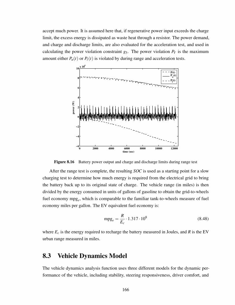
accept much power. It is assumed here that, if regenerative power input exceeds the chargelimit, the excess energy is dissipated as waste heat through a resistor. The power demand,and charge and discharge limits, are also evaluated for the acceleration test, and used incalculating the power violation constraint g5. The power violation PV is the maximumamount either Pu(t) or P (t) is violated by during range and acceleration tests.
0 2000 4000 6000 8000 10000 12000−6
−4
−2
0
2
4
6
8
10 x 104
time (sec)
pow
er (W
)
P(t)Pu(t)
Pl(t)
Figure 8.16 Battery power output and charge and discharge limits during range test
After the range test is complete, the resulting SOC is used as a starting point for a slowcharging test to determine how much energy is required from the electrical grid to bringthe battery back up to its original state of charge. The vehicle range (in miles) is thendivided by the energy consumed in units of gallons of gasoline to obtain the grid-to-wheelsfuel economy mpge, which is comparable to the familiar tank-to-wheels measure of fueleconomy miles per gallon. The EV equivalent fuel economy is:
mpge =REc·1.317 ·108 (8.48)
where Ec is the energy required to recharge the battery measured in Joules, and R is the EVurban range measured in miles.
8.3 Vehicle Dynamics Model
The vehicle dynamics analysis function uses three different models for the dynamic per-formance of the vehicle, including stability, steering responsiveness, driver comfort, and
166
roadholding metrics. A steady-state bicycle model is used to predict directional stability at aconstant speed, and a dynamic bicycle model is used to evaluate steering responsiveness. Aquarter-car model is used to compute metrics for driver comfort, suspension working space,and tire and suspension forces.
8.3.1 Directional Stability
The steering angle of the front tires required to guide a vehicle around a curve of radius Rc
is:
δ f =LRc
+(
Wf
Cα f− Wr
Cαr
)v2
gRc(8.49)
where g is the acceleration of gravity, Wf and Wr are the static forces on the front and reartires, respectively, and Cα f and Cαr are the cornering stiffnesses for the front and rear tires[147]. If the second term of Eq. 8.49 is positive, the steering angle is required to followa curve of radius Rc increases with longitudinal velocity. This is a condition known asundersteer. If the second term of Eq. 8.49 is positive, δ f decreases with velocity. Thisoversteer condition can be unstable if v exceeds the critical velocity:
vcrit =√
gL−Kus
(8.50)
where Kus is the understeer coefficient:
Kus =(
Wf
Cα f− Wr
Cαr
)(8.51)
Since v2/gRc is always positive, Kus ≥ 0 indicates an understeer vehicle. The corneringstiffness values can vary with a number of factors. Here the dependence of corneringstiffness on tire normal force is modeled using a quadratic polynomial fit to empirical datafor the EV fictitious tire [72]:
Cα f = Cα1 +Cα2Wf +Cα3W 2f (8.52)
The parameter values for Eq. (8.52) are given in Table 8.6. The formula for the rearcornering stiffness is similar, but depends on Wr instead. According to this steady-statestability model, directional stability is assured below a maximum intended speed vmax if:
Ds = L+v2
maxgKus
≥ 0 (8.53)
167
8.3.2 Steering Responsiveness
A two DOF second-order model was used to simulate dynamic vehicle motion in the yawplane under steering input at a constant longitudinal velocity. The equations of motion are:
a1vy +a2Ωz +a3vy = a4δ f (t) (8.54a)
b1Ωz +b2Ωz +b3vy = b4δ f (t) (8.54b)
where:
a1 = m
a2 = m+2(`1Cα f − `2Cαr)
v
a3 =2(Cα f +Cαr)
va4 = 2Cα f
b1 = Iz
b2 =2(`2
1Cα f + `22Cαr)
v
b3 =2(`2
1Cα f − `22Cαr)
vb4 = 2`1Cα f
and vy is the lateral vehicle velocity, Ωz is the yaw rate, Iz is the yaw inertia, and δ f (t) isa time-varying steering input. The corresponding state space model is:
[vyΩz
]=
[−a3
a1−a2
a1
−b3b1−b2
b1
][vyΩz
]+
[a4a1b4a1
]δ f (8.55)
The state variable of interest here is the yaw rate. When a vehicle is driving straightahead after a step steering input δ f 0 is applied, the lateral velocity and and yaw rate increasefrom zero and then settle on steady-state nonzero values. A vehicle that approaches itssteady-state yaw rate quickly is considered to be responsive. The yaw rate rise time (tr), i.e.,the time required for the yaw rate to increase from 10% to 90% of its steady state value, isthe metric used to evaluate steering responsiveness. Constraint g8 requires the yaw rate risetime to be less than trmax.
168
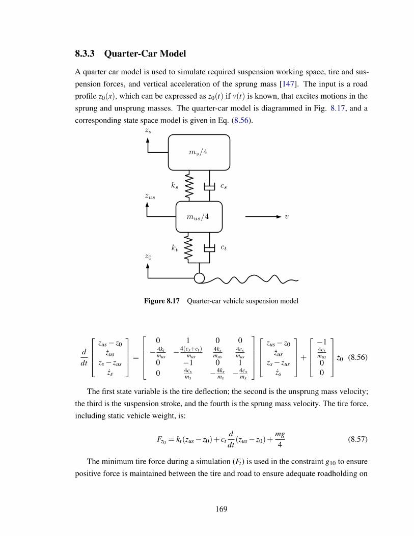
8.3.3 Quarter-Car Model
A quarter car model is used to simulate required suspension working space, tire and sus-pension forces, and vertical acceleration of the sprung mass [147]. The input is a roadprofile z0(x), which can be expressed as z0(t) if v(t) is known, that excites motions in thesprung and unsprung masses. The quarter-car model is diagrammed in Fig. 8.17, and acorresponding state space model is given in Eq. (8.56).
v
ks cs
ktct
z0
zus
zs
ms/4
mus/4
Figure 8.17 Quarter-car vehicle suspension model
ddt
zus− z0
zuszs− zus
zs
=
0 1 0 0− 4kt
mus−4(cs+ct)
mus
4ksmus
4csmus
0 −1 0 10 4cs
ms−4ks
ms−4cs
ms
zus− z0zus
zs− zuszs
+
−14ctmus00
z0 (8.56)
The first state variable is the tire deflection; the second is the unsprung mass velocity;the third is the suspension stroke, and the fourth is the sprung mass velocity. The tire force,including static vehicle weight, is:
Fz0 = kt(zus− z0)+ ctddt
(zus− z0)+mg4
(8.57)
The minimum tire force during a simulation (Ft) is used in the constraint g10 to ensurepositive force is maintained between the tire and road to ensure adequate roadholding on
169

rough terrain and to verify that the tire never loses contact with the road under normal drivingconditions, a requirement for quarter-car model validity. The force that the suspension exertson the sprung mass is:
Fzs =−mszs
4(8.58)
Three different tests are performed using the quarter-car model: a ramp input test, amoderately rough road simulation, and a very rough road simulation. In all tests the tiredamping rate (ct) is assumed to be zero. In the ramp input test the vehicle approaches aramp input at a grade of γ at a velocity of vr0, and the maximum force on the sprung mass(Fs = max(Fzs(t))) is recorded for use in the structural analysis function. The suspensionworking space (δW ) is the largest value of the third state variable during the ramp test, andis used in the constraint g9. The other two tests use stochastic inputs: z0a(x) is the spatialprofile of a moderately rough road, and z0b(x) is the spatial profile of a very rough road.A constant velocity was used with each of these inputs: va0 and vb0. These profiles weregenerated using a gaussian random number generator and a series of filtering steps, and thenanalyzed using standard techniques for the international roughness index (IRI) [120]. Thefirst step is to generate Np = dLp/δpe random data points with a variance of σp, and thenapply a digital filter to remove high-frequency data beyond a spatial cutoff frequency of f0
[12]. The spatial length of the profile is Lp, and the step size in the profile data is δp. Thefilter implemented is:
yn = bxn +ayn−1 (8.59)
where xn and yn are the n-th unfiltered and filtered data points, respectively, and the filtercoefficients are defined as:
a = e−2π f0δp
b = 1− e−2π f0δp
A second type of digital filter is then applied to the data as specified by IRI requirements.This moving average filter is defined by the formula:
yn =1
Nw
n
∑i=n−Nw+1
xi (8.60)
where Nw = dL0/δpe is the number of data points in the filter baselength L0. The profile isthen refined using a finer step size and smoothed using spline interpolation so that inputis more suitable for simulation purposes. A portion of one road profile is illustrated inFig. 8.18, where unfiltered data is displayed alongside profiles generated after the first and
170
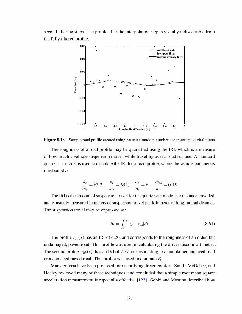
second filtering steps. The profile after the interpolation step is visually indiscernible fromthe fully filtered profile.
0 0.2 0.4 0.6 0.8 1 1.2 1.4 1.6 1.8 2−0.06
−0.04
−0.02
0
0.02
0.04
0.06
Longitudinal Position (m)
Elev
atio
n (m
)
unfiltered datalow−pass filtermoving average filter
Figure 8.18 Sample road profile created using gaussian random number generator and digital filters
The roughness of a road profile may be quantified using the IRI, which is a measureof how much a vehicle suspension moves while traveling over a road surface. A standardquarter-car model is used to calculate the IRI for a road profile, where the vehicle parametersmust satisfy:
ks
ms= 63.3,
kt
ms= 653,
cs
ms= 6,
mus
ms= 0.15
The IRI is the amount of suspension travel for the quarter-car model per distance travelled,and is usually measured in meters of suspension travel per kilometer of longitudinal distance.The suspension travel may be expressed as:
δS =∫ t f
0|zs− zus|dt (8.61)
The profile z0a(x) has an IRI of 4.20, and corresponds to the roughness of an older, butundamaged, paved road. This profile was used in calculating the driver discomfort metric.The second profile, z0b(x), has an IRI of 7.37, corresponding to a maintained unpaved roador a damaged paved road. This profile was used to compute Ft .
Many criteria have been proposed for quantifying driver comfort. Smith, McGehee, andHealey reviewed many of these techniques, and concluded that a simple root mean squareacceleration measurement is especially effective [123]. Gobbi and Mastinu described how
171
to use such a metric in ground vehicle optimization [64]. The metric used here is root meansquare of the power spectral density of the sprung mass acceleration (zs), denoted by az. BS6841 suggests that an az value of up to 0.642 g’s (1g =9.81 m/s2) results in a ride qualitythat is only ‘a little uncomfortable’ [26]. Constraint g11 limits az to 0.80 g while travelingover the profile z0a(x).
Table 8.6 Vehicle dynamics model parametersCα1 -3.68·103 constant cornering stiffness parameterCα2 21.4 linear cornering stiffness parameterCα3 2.70·10−3 quadratic cornering stiffness parameterδ f 0 0.02 rad steering step inputvr0 15.0 m/s ramp test velocityva0 15.0 m/s velocity for stochastic profile avb0 22.2 m/s velocity for stochastic profile bγ 13% ramp test gradef0 0.15 cycle/m filter cutoff frequencyL0 0.25 m filter baselength
8.4 Structural Model
The vehicle structure was modeled as a space frame and analyzed using finite elementanalysis (FEA) [93] to determine the stiffness and stress values for constraints g13–g16. TheFEA model was created using ANSYSTM, and also was used to calculate mass and inertiaproperties of the vehicle frame required as input to the mass distribution and packagingfunction. The vehicle frame model is shown in Fig. 8.19 with the beam element divisionsvisible (911 beam elements in total). The size of frame elements is exaggerated in the figure,and frame members have circular cross sections. The frame material is AISI 4130 steel witha modulus of 205 GPa, Poisson’s ratio of 0.30, and mass density of 7500 kg/m3.
The structural design was simplified by using only two design variables: t f , the wallthickness of all frame members, and d f , the outer diameter of all frame members. Thisdesign variable set requires a compatibility constraint (g12 in Problem (8.2)). The influenceof the battery mass and stiffness is included in this model. Four structural tests are performedto evaluate constraints g13–g16:
1. Torsional stiffness (Ktmin): A moment about the x axis is applied via the rear suspen-sion hardpoints while the front hardpoints are held fixed. The deflection is measured,and then the rotational angle and torsional stiffness is calculated. This stiffness shouldbe at least 12,000 Nm/deg [95].
2. Bending stiffness (Kbmin): the front and rear axles are fixed while a vertical load is
172
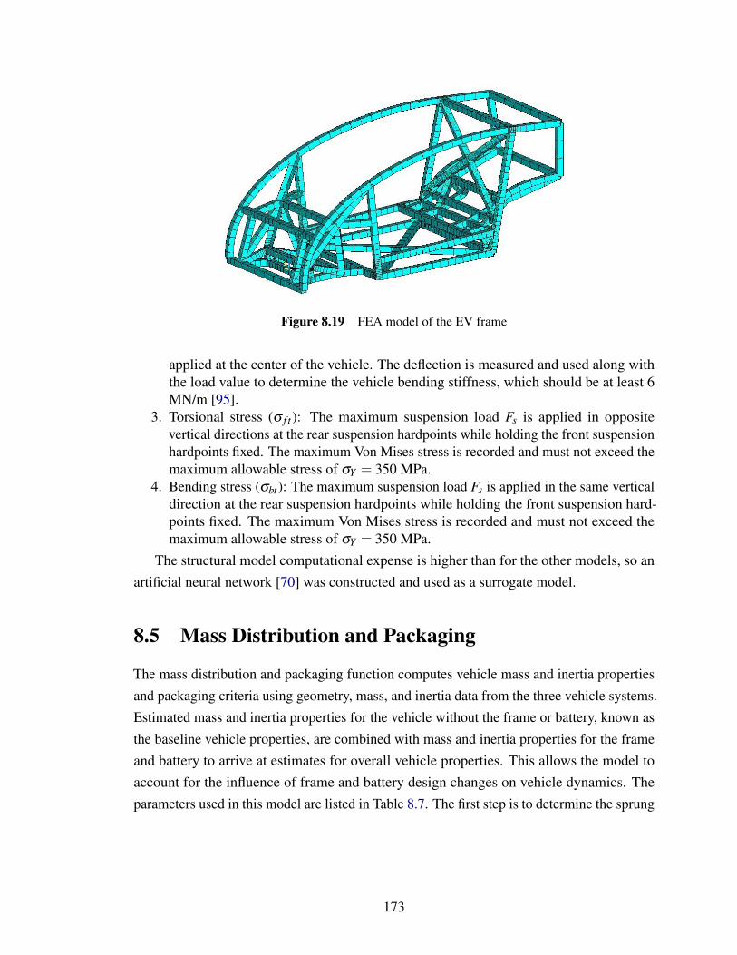
Figure 8.19 FEA model of the EV frame
applied at the center of the vehicle. The deflection is measured and used along withthe load value to determine the vehicle bending stiffness, which should be at least 6MN/m [95].
3. Torsional stress (σ f t): The maximum suspension load Fs is applied in oppositevertical directions at the rear suspension hardpoints while holding the front suspensionhardpoints fixed. The maximum Von Mises stress is recorded and must not exceed themaximum allowable stress of σY = 350 MPa.
4. Bending stress (σbt): The maximum suspension load Fs is applied in the same verticaldirection at the rear suspension hardpoints while holding the front suspension hard-points fixed. The maximum Von Mises stress is recorded and must not exceed themaximum allowable stress of σY = 350 MPa.
The structural model computational expense is higher than for the other models, so anartificial neural network [70] was constructed and used as a surrogate model.
8.5 Mass Distribution and Packaging
The mass distribution and packaging function computes vehicle mass and inertia propertiesand packaging criteria using geometry, mass, and inertia data from the three vehicle systems.Estimated mass and inertia properties for the vehicle without the frame or battery, known asthe baseline vehicle properties, are combined with mass and inertia properties for the frameand battery to arrive at estimates for overall vehicle properties. This allows the model toaccount for the influence of frame and battery design changes on vehicle dynamics. Theparameters used in this model are listed in Table 8.7. The first step is to determine the sprung
173
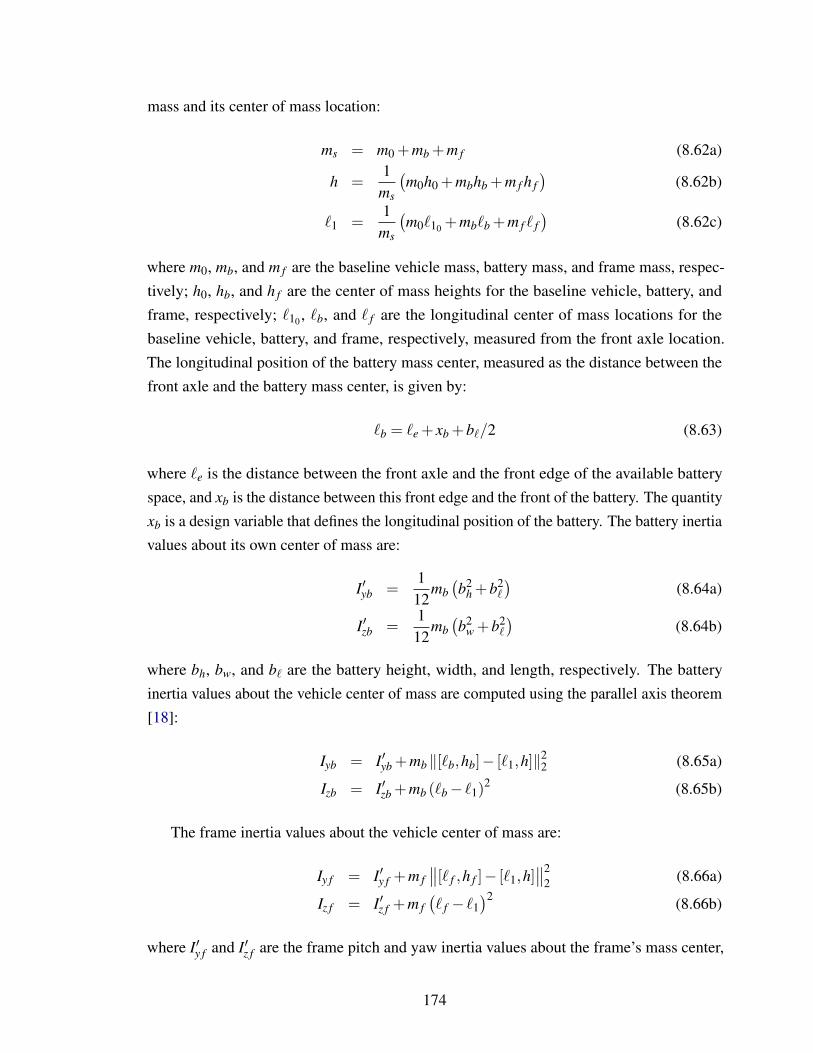
mass and its center of mass location:
ms = m0 +mb +m f (8.62a)
h =1
ms
(m0h0 +mbhb +m f h f
)(8.62b)
`1 =1
ms
(m0`10 +mb`b +m f ` f
)(8.62c)
where m0, mb, and m f are the baseline vehicle mass, battery mass, and frame mass, respec-tively; h0, hb, and h f are the center of mass heights for the baseline vehicle, battery, andframe, respectively; `10 , `b, and ` f are the longitudinal center of mass locations for thebaseline vehicle, battery, and frame, respectively, measured from the front axle location.The longitudinal position of the battery mass center, measured as the distance between thefront axle and the battery mass center, is given by:
`b = `e + xb +b`/2 (8.63)
where `e is the distance between the front axle and the front edge of the available batteryspace, and xb is the distance between this front edge and the front of the battery. The quantityxb is a design variable that defines the longitudinal position of the battery. The battery inertiavalues about its own center of mass are:
I′yb =112
mb(b2
h +b2`
)(8.64a)
I′zb =112
mb(b2
w +b2`
)(8.64b)
where bh, bw, and b` are the battery height, width, and length, respectively. The batteryinertia values about the vehicle center of mass are computed using the parallel axis theorem[18]:
Iyb = I′yb +mb ‖[`b,hb]− [`1,h]‖22 (8.65a)
Izb = I′zb +mb (`b− `1)2 (8.65b)
The frame inertia values about the vehicle center of mass are:
Iy f = I′y f +m f∥∥[` f ,h f ]− [`1,h]
∥∥22 (8.66a)
Iz f = I′z f +m f(` f − `1
)2 (8.66b)
where I′y f and I′z f are the frame pitch and yaw inertia values about the frame’s mass center,
174
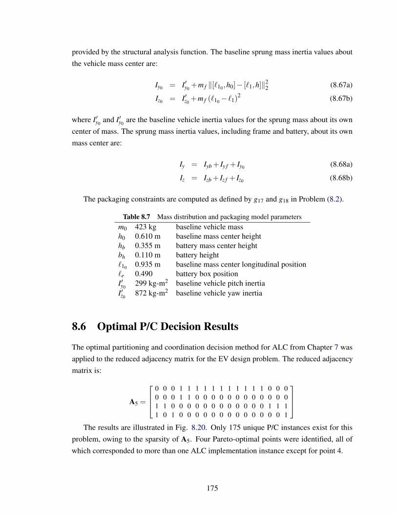
provided by the structural analysis function. The baseline sprung mass inertia values aboutthe vehicle mass center are:
Iy0 = I′y0+m f ‖[`10,h0]− [`1,h]‖2
2 (8.67a)
Iz0 = I′z0+m f (`10− `1)
2 (8.67b)
where I′y0and I′y0
are the baseline vehicle inertia values for the sprung mass about its owncenter of mass. The sprung mass inertia values, including frame and battery, about its ownmass center are:
Iy = Iyb + Iy f + Iy0 (8.68a)
Iz = Izb + Iz f + Iz0 (8.68b)
The packaging constraints are computed as defined by g17 and g18 in Problem (8.2).
Table 8.7 Mass distribution and packaging model parametersm0 423 kg baseline vehicle massh0 0.610 m baseline mass center heighthb 0.355 m battery mass center heightbh 0.110 m battery height`10 0.935 m baseline mass center longitudinal position`e 0.490 battery box positionI′y0
299 kg-m2 baseline vehicle pitch inertiaI′z0
872 kg-m2 baseline vehicle yaw inertia
8.6 Optimal P/C Decision Results
The optimal partitioning and coordination decision method for ALC from Chapter 7 wasapplied to the reduced adjacency matrix for the EV design problem. The reduced adjacencymatrix is:
A5 =
0 0 0 1 1 1 1 1 1 1 1 1 1 1 0 0 00 0 0 1 1 0 0 0 0 0 0 0 0 0 0 0 01 1 0 0 0 0 0 0 0 0 0 0 0 0 1 1 11 0 1 0 0 0 0 0 0 0 0 0 0 0 0 0 1
The results are illustrated in Fig. 8.20. Only 175 unique P/C instances exist for this
problem, owing to the sparsity of A5. Four Pareto-optimal points were identified, all ofwhich corresponded to more than one ALC implementation instance except for point 4.
175
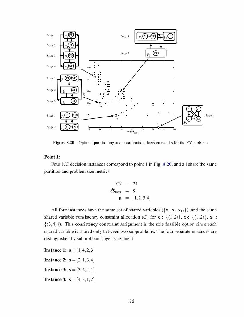
8 10 12 14 16 18 20 22 240
5
10
15
20
25
Avg SSmax
CS
Stage 1
PTP1
VDP2
STP3
MP4
Stage 1
Stage 2
Stage 3
Stage 4
PTP1
VD
P2ST
P3M
Stage 1
Stage 2
Stage 3
PTP1
VDStage 1
Stage 2P2
ST MP1
P1
P3
Stage 1
Stage 2
VDM STP2
PT
PT VD
ST M
1
2
34
5
Figure 8.20 Optimal partitioning and coordination decision results for the EV problem
Point 1:Four P/C decision instances correspond to point 1 in Fig. 8.20, and all share the same
partition and problem size metrics:
CS = 21SSmax = 9
p = [1,2,3,4]
All four instances have the same set of shared variables (x1,x2,x13), and the sameshared variable consistency constraint allocation (Gc for x1: 〈1,2〉, x2: 〈1,2〉, x13:〈3,4〉). This consistency constraint assignment is the sole feasible option since eachshared variable is shared only between two subproblems. The four separate instances aredistinguished by subproblem stage assignment:
Instance 1: s = [1,4,2,3]
Instance 2: s = [2,1,3,4]
Instance 3: s = [3,2,4,1]
Instance 4: s = [4,3,1,2]
176
The ALC implementation for the first instance is illustrated in Fig. 8.20.
Point 2:Three P/C decision instances correspond to point 2, and all share the same partition and
problem size metrics:
CS = 10SSmax = 10
p = [1,1,2,3]
Grouping the powertrain and vehicle dynamics analysis functions together reduces thenumber of external shared variables. All three instances have one shared variable only(x13), and the only possible consistency constraint assignment is 〈2,3〉 for x13. Thesubproblem stage assignment for each instance is as follows:
Instance 1: s = [1,2,3]
Instance 2: s = [2,3,1]
Instance 3: s = [3,1,2]
The ALC implementation for the first instance is illustrated in Fig. 8.20.
Point 3:Two P/C decision instances correspond to point 2, and all share the same partition and
problem size metrics:
CS = 5SSmax = 13
p = [1,1,2,2]
Again, the powertrain and vehicle dynamics analysis functions are placed in the samesubproblem. The third and fourth analysis functions share one design variable, which canbe eliminated from the set of external shared design variables by grouping these analysisfunctions into the same subproblem. Point 3 has no external shared design variables, andtherefore no shared variable consistency constraint assignments. The subproblem stageassignment for each instance is as follows:
Instance 1: s = [1,2]
Instance 2: s = [2,1]
177

The ALC implementation for the first instance is illustrated in Fig. 8.20.
Point 4:The fourth Pareto-optimal point corresponds to the IDF formulation with a single
subproblem. IDF formulations do not have external shared design variables. The problemsize metrics are:
CS = 0SSmax = 21
Point 5:The last point discussed here is not Pareto-optimal, but is included for comparison with
the other points. Point 5 in Fig. 8.20 corresponds to two instances that share the samepartition and problem size metrics:
CS = 15SSmax = 14
p = [1,2,3,2]
Analysis functions two and four are grouped together, but share no design variables, andhave only one coupling variable relationship. This partition does not help reduce CS, andresults in the maximal set of external shared variables: x1,x2,x13. Since these variableslink only two subproblems each, the only consistency constraint allocation option exists(Gc for x1: 〈1,2〉, x2: 〈1,2〉, x13: 〈3,4〉). Point 5 differs from the others in that eachinstance specifies parallel subproblem solution:
Instance 1: s = [1,2,2]
Instance 2: s = [2,1,1]
The second instance is illustrated in Fig. 8.20. The EV problem structure is suchthat parallel subproblem solution does not offer an advantage when CS and SSmax are themetrics used in solving the optimal P/C decision problem. All four Pareto-optimal pointsinvolve serial subproblem solution. Different problem structure, or an alternative CS metricthat penalizes increased stage depth, may change this outcome. The work presented hereestablishes a new approach to constructing distributed optimization problems; further workis required to study metrics used to approximate solution difficulty.
In each Pareto-optimal partition with less than four subproblems, the powertrain andvehicle dynamics analysis functions are grouped together. These functions also share the
178

largest number of design variables between them. Placing a1 and a2 in the same subproblemhas a large impact on reducing the number of external shared design variables. Recall fromChapter 7 that a variable shared between two subproblems requires two separate variablecopies, while coupling variables require only one. These copies increase both coordinationand subproblem size. Therefore, the grouping of a1 and a2 is expected; choosing partitionsthat lead to fewer external shared design variables is a good approach for reducing bothcoordination and subproblem size. This highlights the importance of distinguishing betweenshared and coupling variables, rather than treating all linking variables as shared variables.
Moving from point 4 to point 3 reduces SSmax from 21 to 13, and only requires acoordination problem size of 5. This indicates that the EV problem is a good candidate fordecomposition-based design optimization. Also note that several points exist in Fig. 8.20with SSmax > 21 and CS > 0; these points correspond to exceptionally poor partitions thatincrease both coordination and subproblem size. As we move along the Pareto set startingwith point 1, the number of subproblems increases, which is expected as more emphasis isplaced on reducing CS. Note that the number of instances corresponding to each point alsoincreases as we move toward finer partitions; this is also expected since stage assignmentoptions increase with the number of subproblems.
Each of the 175 P/C instances for the EV problem specifies uniquely an ALC formulation.The formulation for the first instance of point 3 is presented here as an illustration. Theexternal coupling variables in this case are:
y12 = [y14,y24]y21 = [y31,y32,y41]
where:
y14 = [ms,h, `1, Iy]y24 = [ms, `1, Iz]y31 = [bm,bw,b`]y32 = Fs
y41 = [bm,bw,b`]
The coupling variables between analysis functions three and four are internal couplingvariables for subproblem 2:
y43 = [m f ,h f , ` f , Iy f , Iz f ]
The ALC formulation for subproblems 1 and 2 are given in Eqs. (8.69) and (8.69),respectively. S12 and S21 are selection matrices that choose analysis function components
179
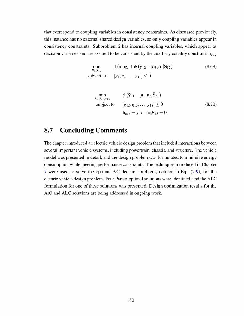
that correspond to coupling variables in consistency constraints. As discussed previously,this instance has no external shared design variables, so only coupling variables appear inconsistency constraints. Subproblem 2 has internal coupling variables, which appear asdecision variables and are assured to be consistent by the auxiliary equality constraint haux.
minx1,y12
1/mpge +φ(y12− [a3,a4]S12
)(8.69)
subject to [g1,g2, . . . ,g11]≤ 0
minx2,y21,y43
φ(y21− [a1,a2]S21
)subject to [g12,g13, . . . ,g18]≤ 0 (8.70)
haux = y43−a3S43 = 0
8.7 Concluding Comments
The chapter introduced an electric vehicle design problem that included interactions betweenseveral important vehicle systems, including powertrain, chassis, and structure. The vehiclemodel was presented in detail, and the design problem was formulated to minimize energyconsumption while meeting performance constraints. The techniques introduced in Chapter7 were used to solve the optimal P/C decision problem, defined in Eq. (7.9), for theelectric vehicle design problem. Four Pareto-optimal solutions were identified, and the ALCformulation for one of these solutions was presented. Design optimization results for theAiO and ALC solutions are being addressed in ongoing work.
180
Chapter 9
Conclusion
9.1 Summary
Many engineering systems are too complex to approach as single large design problems.A usual approach is to partition the system design problem into smaller subproblems thatare more easily solved. These subproblems are coupled through analysis interactions andshared design variables. A coordination strategy is required to account for these interactions,and to help guide iterative solution of subproblems toward a state of consistency, and towarda design that is optimal for the overall system, not just for the individual components.Decomposition-based design optimization techniques utilize optimization algorithms tosolve system subproblems, and coordination algorithms to guide the solution process. Thesetechniques are especially useful when mathematical models exist that can predict systembehavior. This dissertation focused on the case where computer simulations are used as theanalysis functions in the system model.
The difficulty of solving the subproblems and the difficulty of the coordination problemboth contribute to overall solution expense. Both of these factors are influenced by thesystem partition and coordination strategy. Partitioning and coordination decisions mustbe made before a system design problem can be solved using decomposition-based designoptimization. This dissertation was centered on techniques for making partitioning andcoordination decisions using information about problem structure, such as dependencerelationships between analysis functions and on design variables. Previous techniqueshad addressed either the partitioning problem or some form of the coordination decisionproblem, but few had studied partitioning and coordination decisions together. It was shownhere that partitioning and coordination decisions are coupled; this was accomplished bydemonstrating that making partitioning and coordination decisions independently or insequence leads to suboptimal results, while a simultaneous decision approach consistentlyidentified better decisions.
A simultaneous decision approach requires precedence information as well as knowledge
181
of analysis function dependence on design variables. Early methods relied solely onprecedence information to make partitioning decisions; later partitioning methods did notuse directionality in making decisions. The simultaneous partitioning and coordinationdecision methods introduced here use both types of information. The reduced adjacencymatrix was developed specifically to represent this information compactly, and is in aform convenient for computational purposes. The reduced adjacency matrix enables alsocalculation of subproblem optimization dimension; previous methods approximate thisquantity using just the number of analysis functions or variables.
The optimal P/C methods of Chapters 5–7 involved the solution of nonlinear combinato-rial optimization problems, which are NP-complete. Exhaustive enumeration may be usedto solve these problems for small systems, and an evolutionary algorithm was developed forlarger systems. While an efficient algorithm does not yet exist for solving these problems,in practice they can be solved fast enough to be of benefit. Some alternate methods, suchas Michelena’s spectral partitioning method [105], make several simplifying assumptionsthat allow application of very fast solution algorithms. The optimal P/C methods presentedhere are more difficult to solve, but provide a more complete decision model with fewerapproximations. In many cases the design problem solution time vastly exceeds P/C solutiontime, so the more accurate P/C decision methods may be preferable.
Two optimal P/C methods were presented. The first, given in Chapter 5, applies todistributed optimization methods with properties similar to ATC or ALC. The second method,presented in Chapter 7, was developed for a specific class of parallel ALC implementations.This allowed the use of very detailed problem size metrics. More importantly, limiting theP/C decision method to parallel ALC for quasi-separable problems enabled the additionof consistency constraint allocation to the P/C decision method. An automated method forallocating consistency constraints is especially useful for ALC due to its linking structureflexibility. ALC consistency constraints can be adapted to fit the structure of arbitrarynon-hierarchical problems, but the immense number of linking structure options makesmanual decision making impractical. The developed automated technique was required totake advantage of ALC’s flexibility in practice.
Several original engineering design problems were developed to demonstrate conceptsthroughout this dissertation. The majority are described in sufficient detail for replication.An electric water pump design problem and a structural design problem were used indemonstrating P/C decision making without consistency constraint allocation, and an electricvehicle (EV) design problem was developed to demonstrate P/C decision making withconsistency constraint allocation. The EV problem emphasized analysis interactions andshared design variables between vehicle systems.
182
9.2 Extension of Simultaneous P/C Decision Making
The P/C decision methods presented here were developed with an eye toward system designproblems that use simulation-based analysis functions. These problems have known input-output relationships, and normally have quasi-separable problem structures. While thespecific techniques presented here apply to problems that meet these assumptions, the moregeneral principle of simultaneous P/C decision making can be extended to other applications.For example, new decision models can be derived for distributed optimization formulationsother than ATC or ALC, or for problems that are not quasi-separable. The steps for creatinga new decision model are as follows:
1. Identify primary sources of computational expense2. Isolate partitioning and coordination decisions that impact these sources3. Define a set of decision variables for the P/C problem4. Define P/C problem objective function(s)5. Develop a mapping between decision variables and objective functions
Many system optimization methods employ some type of nested approach. ATC andALC have subproblems nested within a fixed point iteration algorithm. Collaborative op-timization and Dantzig-Wolfe decomposition have subproblems nested within a masteroptimization problem. Nested processes generally have two primary sources of computa-tional expense: the inner loop and the outer loop. The methods presented here use CS toestimate outer loop expense, and SSmax or SSmax to model inner loop expense. In a nestedprocess there is a natural tradeoff between these two sources of expense, and it is importantin an optimal P/C method to address this tradeoff. A multi-objective optimization approachis a helpful approach for analyzing such tradeoffs.
This methodology is not limited to decomposition-based design optimization, but canapply to other processes with a nested structure or some type of coordination algorithm.For example, more general parallel computing could benefit from such an approach. Acomputing job must be partitioned into individual computing tasks, and then a schedule forthese tasks must be defined that pays heed to precedence relationships and computationaltime. The details may be very different from decomposition-based design optimization, butas long as the steps above can be followed, a simultaneous partitioning and coordinationdecision method may be constructed for parallel computing applications.
183

9.3 Contributions
1. Partitioning and coordination decisions in decomposition-based design optimizationwere shown to be coupled, and that treating them independently leads to sub-optimalsolution approaches.
2. A method for making optimal partitioning and coordination decisions was developed,and it was shown how this method can also be used to analyze the suitability of adecomposition-based approach for solving a particular system design optimizationproblem. The method employs the reduced adjacency matrix, a new system structurerepresentation that combines functional dependence and precedence informationrequired for making simultaneous P/C decisions.
3. A new evolutionary algorithm was developed that solves the optimal P/C problemfor larger systems. The results of this algorithm compared well against exact resultsobtained using exhaustive enumeration.
4. The Augmented Lagrangian Coordination (ALC) formulation provides tremendousflexibility in problem linking structure. This allows a solution process to be tailored tothe needs of a specific problem. Linking structure theory for ALC was developed, andit was shown that the number of linking structure options is very large. Manual linkingstructure decisions are manageable when based on bi-level or hierarchical structures,but this approach fails to exploit the full benefit of linking structure flexibility inALC. This dissertation put forth a method for automating linking structure decisionsfor ALC in an optimal P/C decision method, enabling system designers to take fulladvantage of ALC.
5. Several original engineering design examples were presented. Sufficient detail wasprovided such that most examples can be replicated. These examples thereforemay be used as a basis for future investigations in decomposition-based designoptimization. These examples are an important contribution because suitable systemdesign examples are notably lacking in the literature.
9.4 Future Work
Evolutionary AlgorithmAn evolutionary algorithm was developed for the general partitioning and coordination
decision method introduced in Chapter 5. This entailed a custom genotype representationfor system partition and subproblem sequence. The more detailed method introduced inChapter 7 for the parallel ALC P/C decision problem involved exhaustive enumeration,and was limited to systems with a maximum of four analysis functions; an evolutionaryalgorithm would increase this upper bound and improve the applicability of this method. Anew genotype representation for stage assignment and consistency constraint allocation isrequired.
184
Adaptive P/C Decision MethodA key assumption throughout this dissertation has been that partitioning and coordination
decisions must be made before solution of the system design problem commences; decisionsmust be made with incomplete or approximate information under this assumption. Tech-niques have been developed for updating parallel processing implementations dynamically,i.e., as more information about the system is gathered, or as solution requirements evolve,the parallel processing approach can be updated accordingly without restarting the solutionprocess. It is proposed that this principle can be applied to partitioning and coordinationdecisions for decomposition-based design optimization. Early on in the solution processrelatively little is known about a system. As the solution process progresses, information canbe gathered and analyzed. These data may be used to determine whether dynamic changesin system partition or coordination strategy would be beneficial.
Alternate Coordination AlgorithmsFixed point iteration, or nonlinear Gauss-Seidel, is a nearly ubiquitous choice for coordi-
nation algorithm for methods similar to ATC or ALC. It is a relatively stable, zeroth-orderalgorithm for solving systems of nonlinear equations. Many other options exist for solvingthe coordination problem, such as successive over-relaxation [71], Newton’s method [43],or Aitken’s method [13]. The effect of these alternative algorithms on system optimizationconvergence should be studied.
Integrated Vehicle DesignThe EV design problem introduced in Chapter 8 is a first step toward a more integrated
approach to vehicle design. Several interactions were included in the design model, butmany more interactions important to vehicle performance could be included. For example,the chassis subproblem could include more sophisticated simulations and vehicle maneuvers,or consider detailed suspension geometry in the design. Commercial software for simulatingvehicle dynamics that is currently available is not amenable to the type of integrationdemonstrated in Chapter 8. Substantial software development is required before an integratedvehicle model is realizable. Another improvement includes a more sophisticated packagingmodel would allow for changes in important vehicle dimensions, such as wheelbase andtrack width, and propagate the effect of these changes throughout the vehicle.
185

Bibliography
[1] NOMADm: Nonlinear Optimization for Mixed vAriables and Derivatives for Matlab.http://www.afit.edu/en/ENC/Faculty/MAbramson/nomadm.html. (Accessed August8, 2005).
[2] M.A. Abramson, C. Audet, and J.E. Dennis Jr. Nonlinear programing with meshadaptive direct searches. SIAG/Optimization Views-and-News, 17(1):2–11, 2006.
[3] N.M. Alexandrov and R.M. Lewis. Algorithmic perspective on problem formulationsin MDO. In the proceedings of the 8th AIAA/USAF/NASA/ISSMO Symposium onMultidisciplinary Analysis and Optimization, Long Beach, CA, Sept. 6–8, 2000.
[4] N.M. Alexandrov and R.M. Lewis. Analytical and computational aspects of col-laborative optimization for multidisciplinary design. AIAA Journal, 40(2):301–309,2002.
[5] J.T. Allison. Complex system optimization: A review of analytical target cascading,collaborative optimization, and other formulations. Master’s thesis, Department ofMechanical Engineering, University of Michigan, 2004.
[6] J.T. Allison, M. Kokkolaras, and P.Y. Papalambros. On selection of single-levelformulations for complex system design optimization. Journal of Mechanical Design,Transactions of the ASME, 129(9), 2007.
[7] J.T. Allison, M. Kokkolaras, M. Zawislak, and P.Y. Papalambros. On the use ofanalytical target cascading and collaborative optimization for complex system design.In the proceedings of the 6th World Conference on Structural and MultidisciplinaryOptimization, Rio de Janeiro, Brazil, May 30–June 3, 2005.
[8] J.T. Allison, B. Roth, M. Kokkolaras, I. Kroo, and P.Y. Papalambros. Aircraftfamily design using decomposition-based methods. In the proceedings of the 11thAIAA/ISSMO Multidisciplinary Analysis and Optimization Conference, Portsmouth,Virginia, Sept. 6–8, 2006.
[9] S. Altus, I. Kroo, and P. Gage. Genetic algorithm for scheduling and decompositionof multidisciplinary design problems. Journal of Mechanical Design, Transactions ofthe ASME, 118(4):486–489, 1996.
[10] S.F. Alyaqout, P.Y. Papalambros, and A.G. Ulsoy. Quantification and use of sys-tem coupling in decomposed design optimization problems. In the proceedings of
186

International Mechanical Engineering Congress and Exposition, November 5-11,2005.
[11] B. Amin. Induction Motors: Analysis and Torque Control. Springer-Verlag, Berlin,2001.
[12] A. Antoniou. Digital Filters: Analysis, Design, and Applications. McGraw-Hill,1993.
[13] I.K. Argyros. Steffensen-aitken methods and implicit functions. Pan AmericanMathematical Journal, 11(1):91–96, 2001.
[14] C. Audet and J.E. Dennis Jr. Mesh adaptive direct search algorithms for constraintoptimization. SIAM Journal on Optimization, 17(1):188–217, 2006.
[15] R.J. Balling and J. Sobieszczanski-Sobieski. Optimization of coupled systems: Acritical overview of approaches. AIAA Journal, 34(1):6–17, 1996.
[16] R.J. Balling and C.A. Wilkinson. Execution of multidisciplinary design optimizationapproaches on common test problems. AIAA Journal, 35(1):178–186, 1997.
[17] J.C. Bean. Genetic algorithms and random keys for sequencing and optimization.ORSA Journal on Computing, 6:154–60, 1994.
[18] A. Bedford and W. Fowler. Engineering Mechanics: Dynamics. Addison Wesley,Menlo Park, CA, 1999.
[19] A. Bedford and W. Fowler. Engineering Mechanics: Statics. Addison Wesley, MenloPark, CA, 1999.
[20] D.P. Bertsekas. Nonlinear Programming. Athena Scientific, Belmont, MA, secondedition, 1999.
[21] D.P. Bertsekas and J.N. Tsitsiklis. Parallel and Distributed Computation: NumericalMethods. Athena Scientific, Belmont, MA, 1997.
[22] D.P. Bertsekas and J.N. Tsitsiklis. Operations Research: An Introduction. PrenticeHall, eighth edition, 2006.
[23] V.Y. Blouin, J.D. Summers, G.M. Fadel, and J. Gu. Intrinsic analysis of decompositionand coordination strategies for complex design problems. In Collection of TechnicalPapers—10th AIAA/ISSMO Multidisciplinary Analysis and Optimization Conference,Aug. 30-Sept. 1, 2004.
[24] B.K. Bose. Modern Power Electronics and AC Drives. Prentice Hall,Inc., UpperSaddle River, NJ, 2002.
[25] R.D. Braun. Collaborative Optimization: An Architecture For Large-Scale DistributedDesign. Ph.D. dissertation, Stanford University, April 1996.
187
[26] British Standards Institution. BS 6841: Measurement and evaluation of humanexposure to whole-body mechanical vibration, 1987.
[27] T.R. Browning. Applying the design structure matrix to system decomposition andintegration problems: a review and new directions. IEEE Transactions on EngineeringManagement, 48(3):292–306, 2001.
[28] S.C. Chapra and R.P. Canale. Numerical Methods for Engineers. McGraw-Hill, thirdedition, 1998.
[29] B. Chen, J. Liu, Y. Zhong, and J. Zhou. Properties of the coupled factors in MDO andtheir application in collaborative optimization. In the Proceedings of DETC’00, ASME2000 Design Engineering Technical Conferences and Computers and Information inEngineering Conference, Baltimore, MD, Sept. 10–13, 2000.
[30] L. Chen, Z. Ding, and S. Li. A formal two-phase method for decomposition ofcomplex design problems. Journal of Mechanical Design, Transactions of the ASME,127(2):184–195, 2005.
[31] L. Chen and S. Li. Analysis of decomposability and complexity for design problemsin the context of decomposition. Journal of Mechanical Design, Transactions of theASME, 127(4):545–557, 2005.
[32] F.H. Clarke. Generalized gradients and applications. Transactions of the AmericanMathematical Society, 205:247–262, 1975.
[33] Global Climate and Energy Project. A technical assessment of high-energy batteriesfor light-duty electric vehicles. Technical report, Stanford University, 2006.
[34] Wells Manufacturing Corp. Making sense of engine airflow. Counterpoint: TheElectronic Diagnostic and Driveability Resource, 3(3):1–3, 1999.
[35] E.J. Cramer, J.E. Dennis Jr., P.D. Frank, R.M. Lewis, and G.R. Shubin. Problemformulation for multidisciplinary optimization. SIAM Journal of Optimization, 4:754–776, 1994.
[36] R.L. Daft. Organization Theory and Design. Thomson South-Western, Ohio, eigthedition, 2004.
[37] G.B. Dantzig. Linear Programming and Extensions. Princeton University Press,Princeton, NJ, 1963.
[38] G.B. Dantzig and P. Wolfe. The decomposition principle for linear programs. Opera-tions Research, 8:101–111, 1960.
[39] Davies Craig PTY. LTD., Electric Water Pump Catalogue.www.daviescraig.com.au, (Accessed nov. 8, 2007).
[40] K.A. De Jong. Genetic algorithms are not function optimizers. In the proceedings ofFoundations of Genetic Algorithms 2, San Mateo, CA, 1993 1993.
188
[41] V. DeMiguel and W. Murray. An analysis of collaborative optimization methods. Inthe proceedings of the 8th AIAA/USAF/NASA/ISSMO Symposium on MultidisciplinaryAnalysis and Optimization, Long Beach, CA, Sept. 6–8, 2000.
[42] V. DeMiguel and W. Murray. A local convergence analysis of bilevel decompositionalgorithms. Optimization and Engineering, 7(2):99–133, 2006.
[43] J.E. Dennis Jr. and R.B. Schnabel. Numerical Methods for Unconstrained Optimiza-tion and Nonlinear Equations. SIAM, Philadelphia, 1996.
[44] U.S. Department of Transportation. 2001 National Household Travel Survey, Bureauof Transportation Statistics.www.bts.gov/programs/national_household_travel_survey.
[45] PNGV Battery Test Manual Revision 3, DOE/ID-10597, Feburary 2001.
[46] M. Doyle, T.H. Fuller, and J. Newman. Modeling of galvanostatic charge anddischarge of the lithium/polymer/insertion cell. Journal of The ElectrochemicalSociety, 140(6):1526–1533, 1993.
[47] M. Dragan. On decomposing large sparse systems of nonlinear equations. In theproceedings of the 4th International Workshop on Symbolic and Numeric Algorithmsfor Scientific Computing, Timisoara, Romania, October 9-12, 2002 2002.
[48] A.E. Eiben. Evolutionary computing: the most powerful problem solver in theuniverse? Dutch Mathematical Archive, 5/3(2):126–131, 2002.
[49] A.E. Eiben and J.E. Smith. Introduction to Evolutionary Computing. Springer-Verlag,Germany, 2003.
[50] R. Fellini. A Model-Based Methodology for Product Family Design. Ph.D. disserta-tion, University of Michigan, 2003.
[51] R. Fellini, M. Kokkolaras, N. Michelena, P. Papalambros, A. Perez-Duarte, K Saitou,and P. Feynes. A sensitivity-based commonality strategy for family products of mildvariation, with application to automotive body structures. Structural and Multidisci-plinary Optimization, 27:89–96, 2004.
[52] R. Fellini, M. Kokkolaras, P. Y. Papalambros, and A. Perez-Duarte. Platform selec-tion under performance bounds in optimal design of product families. Journal ofMechanical Design, Transactions Of the ASME, 127(4):524–535, 2005.
[53] R. Fellini, M. Kokkolaras, and P.Y. Papalambros. Quantitative platform selectionin optimal design of product families, with application to automotive engine design.Journal of Engineering Design, 17(5):429–446, 2006.
[54] L.J. Fogel, A.J. Owens, and M.J. Walsh. Artificial intelligence through a simula-tion of evolution. In Biophysics and Cybernetic Systems, pages 131–156. Spartan,Washington DC, 1965.
189

[55] American Institute for Aeronautics and Astronautics Inc. (AIAA). Current state ofthe art in multidisciplinary design optimization. Technical report, MDO TechnicalCommittee, 1991.
[56] T.H. Fuller, M. Doyle, and J. Newman. Simulation and optimization of the duallithium ion insertion cell. Journal of The Electrochemical Society, 141(1):1–10, 1994.
[57] University of Michigan, Aerospace Engineering display. Francois-Xavier BagnoudBuilding. April, 2006.
[58] T.B. Gage and M.A. Bogdanoff. Low-emission range extender for electric vehicles.In R.K. Jurgen, editor, Electric and Hybrid-Electric Vehicles. SAE International,2002.
[59] J.M. Gere. Mechanics of Materials. Brooks/Cole, Pacific Grove, CA, fifth edition,2001.
[60] J.F. Gieras and M. Wing. Permanent Magnet Motor Technology. Marcel Dekker, Inc.,New York, 2002.
[61] J.P. Giesing and J.M. Barthelemy. A summary of industry MDO applications andneeds, 1998. AIAA Paper 98-4737.
[62] M. Giger and P. Ermanni. Evolutionary truss topology optimization using a graph-based parameterization concept. Structural and Multidisciplinary Optimization,32(4):313–326, 2006.
[63] Robert Bosch Gmbh. BOSCH Automotive Handbook. John Wiley and Sons, sixthedition, 2004.
[64] M. Gobbi and G. Mastinu. Analytical description and optimization of the dynamicbehaviour of passively suspended road vehicles. Journal of Sound and Vibration,245(3):457–481, 2001.
[65] D.E. Goldberg. Genetic Algorithms in Search, Optimization, and Machine Learning.Addison-Wesley, 1989.
[66] R. Haftka, J. Sobieszczanski-Sobieski, and S.L. Padula. On options for interdis-ciplinary analysis and design optimization. Structural Optimization, 4(2):65–74,1992.
[67] R. Haftka and L. Watson. Multidisciplinary design optimization with quasiseparablesubsystems. Optimization and Engineering, 6:9–20, 2005.
[68] J. Han. Sequential Linear Programming Coordination Strategy for Deterministicand Probabilistic Analytical Target Cascading. Ph.D. dissertation, University ofMichigan, 2008.
[69] S.P. Han. Superlinearly convergent variable metric algorithms for general nonlinearprogramming problems. Mathematical Programming, 11:263–282, 1976.
190
[70] S. Haykin. Neural Networks: A Comprehensive Foundation. Prentice Hall, secondedition, 1998.
[71] F.B. Hildebrand. Introduction to Numerical Analysis. McGraw-Hill, New York,second edition, 1974.
[72] H. Hisashi. Bridgestone Corporation, personal communication, August 2007.
[73] J.H. Holland. Adaptation in Natural and Artificial Systems. The University ofMichigan Press, Ann Arbor, MI, 1975.
[74] K.F. Hulme and C.L. Bloebaum. Simulation-based comparison of multidisciplinarydesign optimization solution strategies using cascade. Structural and Multidisci-plinary Optimization, 19(1):17–35, 2000.
[75] F.P. Incropera and D.P. DeWitt. Introduction to Heat Transfer. John Wiley and Sons,2002.
[76] G.J.A. Karsemakers. Numerical investigation of two multidisciplinary engineeringdesign problems using the augmented lagrangian coordination method. Technicalreport, Technische Universiteit Eindhoven, 2007.
[77] J.G. Kassakian. Future of power electronics in advanced automotive electrical systems.In the proceedings of the IEEE Annual Power Electronics Specialists Conference,pages 7–14, 1996.
[78] T. Kenjo and S. Nagamori. Permanent-Magnet and Brushless DC Motors. OxfordUniversity Press, New York, 1985.
[79] H.M. Kim. Target Cascading in Optimal System Design. Ph.D. dissertation, Univer-sity of Michigan, 2001.
[80] H.M. Kim, N.F. Michelena, P.Y. Papalambros, and T. Jiang. Target cascading inoptimal system design. Journal of Mechanical Design, Transactions of the ASME,125(3):474–480, 2003.
[81] C.S. Kirkpatrick, C.D. Gelatt Jr., and M. P. Vecchi. Optimization by simulatedannealing. Science, 220(4598):671–680, May 1983.
[82] M. Kokkolaras, Z. Mourelatos, L. Louca, Z. Filipi, G. Delagrammatikas, A. Ste-fanopoulou, P.Y. Papalambros, and D. Assanis. Design under uncertainty and assess-ment of performance reliability of a dual-use medium truck with hydraulic-hybridpowertrain and fuel cell auxiliary power unit. SAE 2005 Transactions: Journal of Pas-senger Cars - Mechanical Systems, 2006. (Selected from the Proceedings of the SAEWorld Congress, April 11–14, 2005, Detroit, Michigan, paper no. 2005-01-1396).
[83] J.R. Koza. Genetic Programming. MIT Press, Cambridge, MA, 1992.
191
[84] R.S. Krishnamachari and P.Y. Papalambros. Optimal hierarchical decompositionsynthesis using integer programming. Journal of Mechanical Design, Transactionsof the ASME, 119(4):440–447, 1997.
[85] I. Kroo, S. Altus, R. Braun, P. Gage, and I. Sobieski. Multidisciplinary opti-mization methods for aircraft preliminary design. In the Proceedings of the 5thAIAA/USAF/NASA/ISSMO Symposium on Multidisciplinary Analysis and Optimiza-tion, pages 697–707, Panama City Beach, FL, Sept. 7–9 1994.
[86] I.M. Kroo. AA241—Aircraft Design: Synthesis and Analysis. Course Notes,http://adg.stanford.edu/aa241/AircraftDesign.html. (Ac-cessed May 27, 2005).
[87] I.M. Kroo. An interactive system for aircraft design and optimization. In theproceedings of the AIAA Aerospace Design Conference, Irvine, CA, Feb. 3–6 1992.
[88] A. Kusiak and N. Larson. Decomposition and representation methods in mechanicaldesign. Journal of Mechanical Design, Transactions of the ASME, 117B:17–24,1995.
[89] A. Kusiak and J. Wang. Decomposition of the design process. Journal of MechanicalDesign, Transactions of the ASME, 115(4):687–695, 1993.
[90] J. Larminie and J. Lowry. Electric Vehicle Technology Explained. John Wiley andSons, Chichester, 2003.
[91] L.S. Lasdon, A.D. Waren, A. Jain, and M. Ratner. Design and testing of a gener-alized reduced gradient code for nonlinear programming. ACM Transactions onMathematical Software, 4(1):34–50, 1978.
[92] J.G. Lin. Analysis and enhancement of collaborative optimization for multidisci-plinary design. AIAA Journal, 42(2):348–360, 2004.
[93] D.L. Logan. A First Course in the Finite Element Method. Brooks/Cole, PacificGrove, CA, third edition, 2002.
[94] A.K. Mackworth. Consistency in networks of relations. Artificial Intelligence,8(1):99–118, 02/ 1977.
[95] D.E. Malen. Fundamentals of auto body structure design. ME513/AUTO513/MFG513 Course Packet, University of Michigan, 2005.
[96] J. Markish. Valuation techniques for commercial aircraft program design. Master’sthesis, Massachusetts Institute of Technology, June 2002.
[97] Matweb material property data. http://www.matweb.com. Accessed April 9, 2004.
[98] P.J. McCleer. Electric drives for pump, fan, and compressor loads in automotiveapplications. In the Proceedings of the IEEE International Symposium on IndustrialElectronics, pages 80–85, Jul. 10–14 1995.
192
[99] C. Meier, A.A. Yassine, and T.R. Browning. Design process sequencing with compe-tent genetic algorithms. Journal of Mechanical Design, Transactions of the ASME,129(6):566–585, 2007.
[100] P.H. Mellor, D. Roberts, and D.R. Turner. Lumped parameter thermal model forelectrical machines of TEFC design. IEE Proceedings B: Electric Power Applications,138(5):205–218, 1991.
[101] M. Meyer and A. Lehnerd. The Power of Product Platforms. New York: IrwinProfessional Publishing, 1997.
[102] J.J. Michalek and P.Y. Papalambros. An efficient weighting update method to achieveacceptable consistency deviation in analytical target cascading. Journal of MechanicalDesign, Transactions Of the ASME, 127(2):206–214, 2005.
[103] N.F. Michelena and P.Y. Papalambros. Network reliability approach to optimaldecomposition of design problems. Journal of Mechanical Design, Transactions ofthe ASME, 117(3):433–440, 1995.
[104] N.F. Michelena and P.Y. Papalambros. Optimal model-based decomposition ofpowertrain system design. Journal of Mechanical Design, Transactions of the ASME,117(4):499–505, 1995.
[105] N.F. Michelena and P.Y. Papalambros. A hypergraph framework for optimal model-based decomposition of design problems. Computational Optimization and Applica-tions, 8(2):173–196, 1997.
[106] N.F. Michelena, H. Park, and P.Y. Papalambros. Convergence properties of analyticaltarget cascading. AIAA Journal, 41(5):897–905, 2003.
[107] U. Montanari. Networks of constraints: Fundamental properties and applications topicture processing. Information Sciences, 7:95–132, 1974.
[108] E. Oberg, F.D. Jones, H.L. Horton, and H Ryffel, H. Machinery’s Handbook. Indus-trial Press Inc., New York, 26th edition, 2000.
[109] J. Oxley. What is a matroid? Cubo Matematica Educacional, 5(3):179–218, 2003.
[110] P.Y. Papalambros and D.J. Wilde. Principles of Optimal Design: Modeling andComputation. Cambridge University Press, New York, second edition, 2000.
[111] M.J.D. Powell. A fast algorithm for nonlinearly constrained optimisation calculations.In G.A. Watson, editor, Numerical Analysis Dundee, pages 144–157. Springer-Verlag,Berlin, 1977.
[112] D.P. Raymer. Aircraft Design: A Conceptual Approach. AIAA Educational Series,third edition, 1999.
[113] I. Rechenberg. Evolutionstrategie: Optimierung Technisher Systeme nach Prinzipiendes Biologischen Evolution. Fromman-Holzlboog Verlag, Stuttgart, 1973.
193

[114] J. L. Rogers and C. L. Bloebaum. Ordering design tasks based on coupling strengths.In the proceedings of the 5th AIAA/USAF/NASA/ISSMO Symposium on Multidisci-plinary Analysis and Optimization, Panama City Beach, FL, Sept. 7–9 1994.
[115] J.L. Rogers. DeMAID—a design manager’s aid for intelligent decomposition user’sguide. Technical Report TM-101575, NASA, 1989.
[116] J.L. Rogers. DeMAID/GA - an enhanced design manager’s aid for intelligent decom-position (genetic algorithms). In the Proceedings of the 6th AIAA/USAF/NASA/ISSMOSymposium on Multidisciplinary Analysis and Optimization, pages 1497–1504, Seat-tle, WA, Sept. 4–6, 1996.
[117] P. J. Rohl, B. He, and P. M. Finnigan. A collaborative optimization environment forturbine engine development. In the Proceedings of the 7th AIAA/USAF/NASA/ISSMOSymposium on Multidisciplinary Analysis and Optimization, St. Louis, MO, Sept.2–4 1998.
[118] F. Rothlauf. Representations for Genetic and Evolutionary Algorithms. Springer-Verlag, Berlin, second edition, 2006.
[119] F. Rothlauf, D.E. Goldberg, and A. Heinzl. Network random keys - a tree represen-tation scheme for genetic and evolutionary algorithms. Evolutionary Computation,10(1):75–97, 2002.
[120] M.W. Sayers and S.M. Karamihas. The little book of profiling. Technical report,University of Michigan Transportation Research Institute, 1998.
[121] B. Scrosati. Lithium rocking chair batteries: An old concept? Journal of TheElectrochemical Society, 139(10):2776–2781, 1992.
[122] P. Seibel. Practical Common Lisp. Apress, Berkley,CA, 2005.
[123] C.C. Smith, D.Y. McGehee, and A.J. Healey. The prediction of passenger ridingcomfort from acceleration data. Journal of Dynamic Systems, Transactions of theASME, 100:34–41, 1978.
[124] L.V. Snyder and M.S. Daskin. A random-key genetic algorithm for the generalizedtraveling salesman problem. European Journal of Operational Research, 174(1):38–53, 2006.
[125] I. Sobieski and I. Kroo. Collaborative optimization using response surface estimation.AIAA Journal, 38(10):1931–1938, 2000.
[126] J. Sobieszczanski-Sobieski. Optimization by decomposition: A step from hierarchicto non-hierarchic systems. In the Proceedings of the 2nd NASA/USAF Symposiumon Recent Advances in Multidisciplinary Analysis and Optimization, Hampton, VA,Sept. 28–30 1988.
194
[127] J. Sobieszczanski-Sobieski, J.S. Agte, and R.R.J. Sandusky. Bilevel integrated systemsynthesis. AIAA Journal, 38(1):164–172, 2000.
[128] J. Sobieszczanski-Sobieski and R.T. Haftka. Multidisciplinary aerospace designoptimization: Survey of recent developments. Structural Optimization, 14(1):1–23,1997.
[129] A.J. Soper, C. Walshaw, and M. Cross. A combined evolutionary search and multi-level optimisation approach to graph-partitioning. Journal of Global Optimization,29(2):225–241, 2004.
[130] J.C. Spall. Introduction to Stochastic Search and Optimization: Estimation, Simula-tion, and Control. Wiley-Interscience, 2003.
[131] D. Stanton and D. White. Constructive Combinatorics. Springer-Verlag, New York,1986.
[132] D.V. Steward. Partitioning and tearing systems of equations. J. SIAM NumericalAnalysis Ser. B, 2(2):345–365, 1965.
[133] D.V. Steward. The design structure system: a method for managing the design ofcomplex systems. IEEE Transactions on Engineering Management, EM-28(3):71–4,1981.
[134] D.V. Steward. Systems analysis and management: structure, strategy, design. Petro-celli Books, Inc., 1981.
[135] N.P. Suh. The principles of design. Oxford University Press, New York, 1990.
[136] L.P. Sullivan. Quality function deployment. Quality Progress, 19(6):39–50, 1986.
[137] B. Surampudi, J. Redfield, G. Ray, A. Montemayor, M. Walls, H. McKee, T. Edwards,and M. Lasecki. Electrification and integration of accessories on a class-8 tractor. Inthe proceedings of the SAE World Congress, Detroit, MI, April 11–14 2005.
[138] R. Thareja and R. Haftka. Numerical difficulties associated with using equality con-straints to achieve multi-level decomposition in structural optimization. In Collectionof Technical Papers - AIAA/ASME/ASCE/AHS 27th Structures, Structural Dynamicsand Materials Conference. Part 1: Structures and Materials., 1986.
[139] S. Tosserams. Analytical target cascading: convergence improvement by sub-problempost-optimality sensitivities. Master’s thesis, Eindhoven University of Technology,2004.
[140] S. Tosserams, L.F.P. Etman, P.Y. Papalambros, and J.E. Rooda. An augmentedLagrangian relaxation for analytical target cascading using the alternating directionmethod of multipliers. Structural and Multidisciplinary Optimization, 31(3):176–189,2006.
195
[141] S. Tosserams, L.F.P. Etman, and J.E. Rooda. Augmented Lagrangian coordinationfor distributed optimal design in MDO. To appear in the International Journal forNumerical Methods in Engineering, 2007.
[142] S. Tosserams, L.F.P. Etman, and J.E. Rooda. An augmented Lagrangian decomposi-tion method for quasiseparable problems in MDO. Structural and MultidisciplinaryOptimization, 34(3), 2007.
[143] E. Tsang. Foundations of constraint satisfaction. Academic Press, San Diego, 1993.
[144] J. Tuzson. Centrifugal Pump Design. John Wiley and Sons, New York, 2000.
[145] T.C. Wagner. A General Decomposition Methodology For Optimal System Design.Ph.D. dissertation, University of Michigan, 1993.
[146] D.H. Wolpert and W.G. Macready. No free lunch theorem for optimisation. IEEETransactions on Evolutionary Computation, 1(1):67–82, 1997.
[147] J.Y. Wong. Theory of Ground Vehicles. John Wiley and Sons, New York, third edition,2001.
196
Related Documents