Optimal parallel scheduling of M-way join queries

hfbrmarion Sysfems Vol. 16, No. 6. pp. 627-639, 1991 0306-4379/91 $3.00 + 0.00 Printed in Great Britain. All rights reserved Copyright 0 1991 Pergamon Press plc

OPTIMAL PARALLEL SCHEDULING OF M-way JOIN QUERIES

FARSHAD FOTOUHI, JASON LEIGH and SATYENDRA P. RANA?

Computer Science Department, Wayne State University, Detroit, MI 48202, U.S.A.

(Received 25 June 1990; in revised form 3 April 1991)

Abstract-The problem of computing multirelation (M-way) join queries on uniprocessor architectures has been considered by many researchers in the past. This paper lays the necessary foundation for work involving optimization of M-way joins in parallel architectures. We explain the inadequacies of previous uniprocessor strategies and describe a more suitable formulation based on the concept of matching in graph theory to approach the problem in a parallel environment. It has been shown that the problem of optimizing M-way joins is an NP-hard problem and hence we would expect that in a parallel processing environment the search space of possible solutions (join schedules) would be enormous, especially when a variable number of processors are considered. Our strategy seeks to reduce the region to search by partitioning the search space according to the number of available processors. Based on this a significant portion of the search space, which will produce non-optimal join schedules, may be ignored.

Key words: Relational join, join schedule, parallel processing, M-way join

1. INTRODUCTION

The relational join is one of the most important and time consuming operations in a relational database system. The join operation between two relations is the cross-referencing of matching tuples of the two joining relations.

There are essentially two types of join operations, theta (0) joins and natural joins. Formally, the theta join between two relations r and s, denoted by r wes is defined as aO(r x s); where x is the Cartesian product, ~7 is the relational algebra’s selection operator and 8 is some predicate on which to select. The natural join between two relations r and s (written as r w s) whose schemas are R and S is defined as: nRUS(r w,-*, =s.A,r.,,,hT.An=J.A,~) where RvS = A,, . . . , A,,, and A, is an attribute.

The join is an important operation because it allows the user to navigate through the database and also techniques used for performing the join are applicable in performing many similar binary operations such as aggregate functions. The join is time consuming because it requires a large amount of cross-referencing between tuples of different relations. The efficiency of the join operation, thus has a deterministic effect on a database system’s performance and as a result has been the subject of intensive study in the development of relational database systems.

I. 1. M-Way join

The M-way join is a join operation that occurs between more than two relations. Typically this is achieved by successively joining two relations at a time until all the M relations have been joined.

The importance of M-way join queries has already been realized in non-traditional database applications. For example, in knowledge base or expert systems using relational systems for storage of persistant data, the need for performing hundreds of joins is not uncommon. Object-oriented database systems, for instance, Iris [l], which use relational systems storage of information, is another class of potential applications generating many joins [2].

Numerous approaches for performing join efficiently have been proposed in the literature [3-61. Most of the existing work pertains to join of two relations, but not much has been done to improve the performance of queries involving join among multiple ( > 2) relations, or so called M-way joins.

tTo whom correspondence should be addressed.

627

628 FARSHAD FOTOUHI et al.

In fact, Ibaraki and Kameda [7] have shown that the problem of optimizing M-way join queries for large M is a hard combinatorial optimization problem. Heuristics such as those for System R and INGRES have been proposed which are based on decomposing an M-way join query into a set of 2-way joins and then determining a near optimal order of join execution, which result in minimum overall evaluation cost. Note that the order in which the interim 2-way joins are performed affects the cost of execution of the query. In other words, the execution cost of the query not only depends on the sizes and number of specified relations, but also on the transient relations to be created as dictated by the decomposition. For a uniprocessor environment, the above approach may be satisfactory, however, in a multiprocessor environment where there is potential for parallel execution, it is advantageous to divide a query into multiple tasks which can run on all the processors in parallel.

2. JOIN PROCESSING TREES AND JOIN SCHEDULES

As the availability of commercial multiprocessor architectures increases, better algorithms must be developed to efficiently perform joins by exploiting the benefits of multiple processors. This paper discusses the issue of optimal ordering of M-way joins in multiprocessor environments. Note that here we are concerned with the order in which the relations are to be joined and not with the specific join method to be used for performing each join. A schedule is therefore an explicit representation of such an ordering. An optimal schedule may be described as a join order that minimizes response time, and/or total cost. Here we represent an M-way join query by a Join Graph.

Given a query Q with the qualification Q = q, A q2 A. . . A q,, on a database LIB with relations

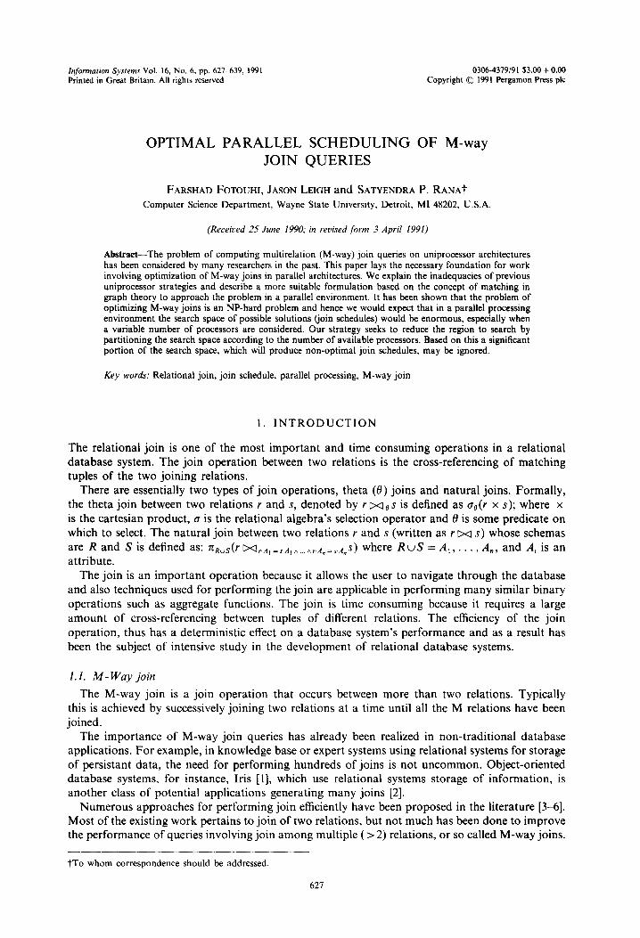
R,,R,,..., R,, we define a join graph as an undirected graph where the nodes represent the join participating relations and the edges between nodes represent a sub-qualification qi; we assume sub-qualifications to be of the form: Ri. attr (where attr is the join attribute). For example, the join graph for the query Q=(R,.a=R,.a)r\(R,.b=R4.b)~(R,.c=R,.c)~(R,.d= R, . d) A (R6. e = R, . e) A (R, -f = R, .f) A (R, . g = R, * g) is shown in Fig. 1 (for simplicity the labeling of the individual edges with the join attributes is omitted in later figures).

The problem which has been previously considered by many researchers [2, 81 is to discover means of determining the optimal join schedule for a uniprocessor architectural model. In their work, the join schedule is represented by a Join Processing Tree (JPT). In addition suggestions have been made that a pipelined join processor be incorporated in the process. A pipelined join is a join that occurs between more than two relations at a time. In the next section we discuss JPTs and their relationship with join schedules.

2.1. JPTs

A JPT is a tree in which each non-leaf node is a join node and each leaf node is a base relation [2]. The join node is formed by joining off its children, which may consist of base relations, intermediate relations, and/or a combination of both. Note that the join node also corresponds to an intermediate relation.

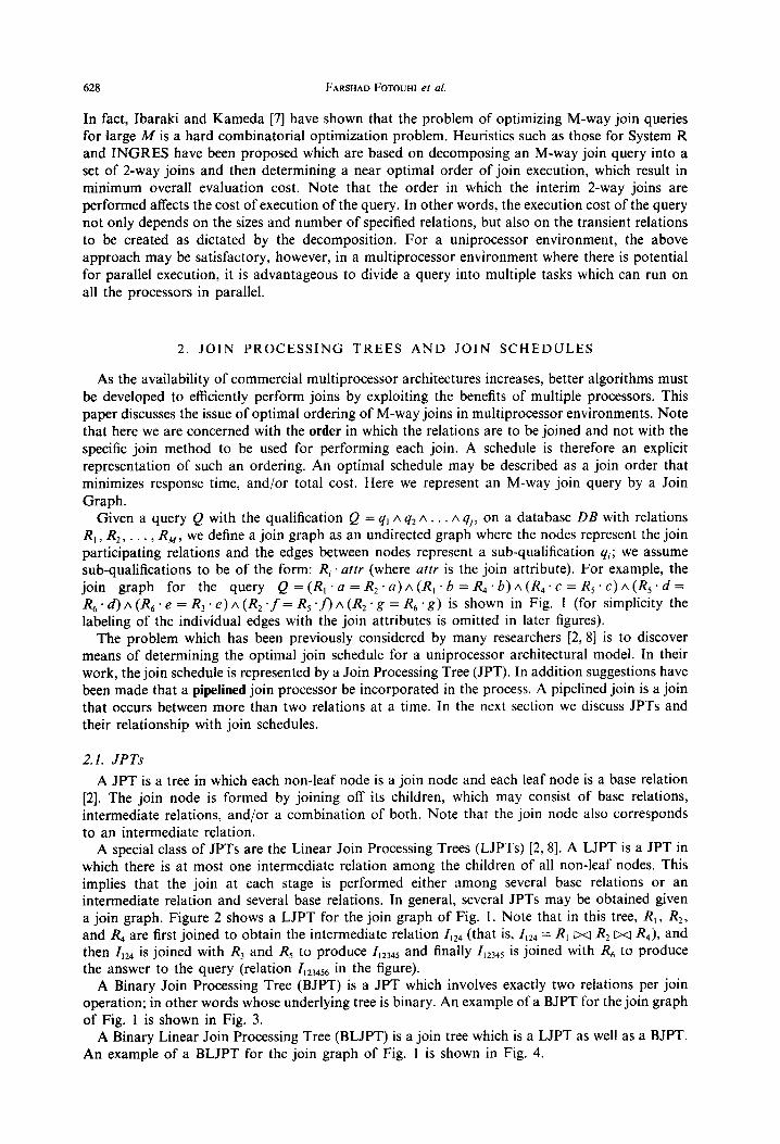
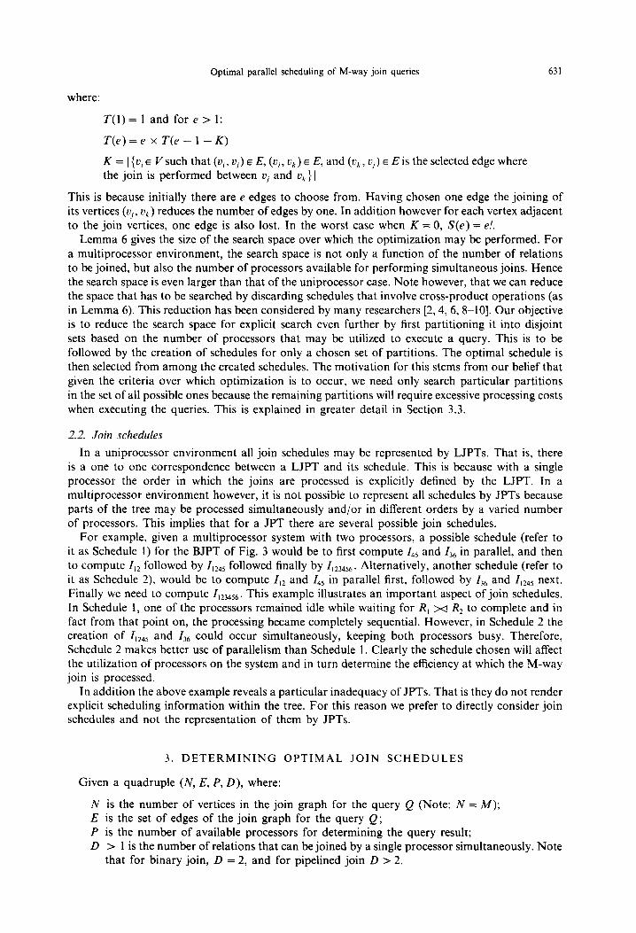
A special class of JPTs are the Linear Join Processing Trees (LJPTs) [2,8]. A LJPT is a JPT in which there is at most one intermediate relation among the children of all non-leaf nodes. This implies that the join at each stage is performed either among several base relations or an intermediate relation and several base relations. In general, several JPTs may be obtained given a join graph. Figure 2 shows a LJPT for the join graph of Fig. 1. Note that in this tree, R, , R,, and R4 are first joined to obtain the intermediate relation I,,, (that is, Z,,, = R, w R, w R4), and then I,,, is joined with R, and R, to produce I,2345 and finally Z,2345 is joined with R, to produce the answer to the query (relation Z,23456 in the figure).

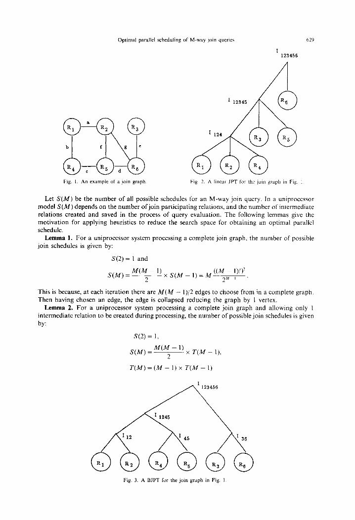
A Binary Join Processing Tree (BJPT) is a JPT which involves exactly two relations per join operation; in other words whose underlying tree is binary. An example of a BJPT for the join graph of Fig. 1 is shown in Fig. 3.

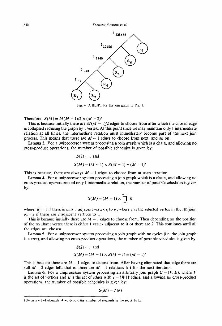
A Binary Linear Join Processing Tree (BLJPT) is a join tree which is a LJPT as well as a BJPT. An example of a BLJPT for the join graph of Fig. 1 is shown in Fig. 4.

Optimal parallel scheduling of M-way join queries

I 123456

629

Fig. I. An example of a join graph. Fig. 2. A linear JPT for the join graph in Fig. I

Let S(M) be the number of all possible schedules for an M-way join query. In a uniprocessor

model S(M) depends on the number of join participating relations, and the number of intermediate relations created and saved in the process of query evaluation. The following lemmas give the motivation for applying heuristics to reduce the search space for obtaining an optimal parallel schedule.

Lemma 1. For a uniprocessor system processing a complete join graph, the number of possible

join schedules is given by:

S(2) = 1 and

M(M - 1) S(M)= *

((A4 - l)!)* xS(M-l)=M 2”_, .

This is because, at each iteration there are M(A4 - I)/2 edges to choose from in a complete graph. Then having chosen an edge, the edge is collapsed reducing the graph by 1 vertex.

Lemma 2. For a uniprocessor system processing a complete join graph and allowing only I intermediate relation to be created during processing, the number of possible join schedules is given by:

S(2) = 1,

M(M-1) wo= 2 x T(M - 1)

T(M)=(M-l)xT(M-1)

Fig. 3. A BJPT for the join graph in Fig. 1.

630 FARSHAD FOTOUHI et al.

Fig. 4. A BLJPT for the join graph in Fig. I.

Therefore: S(M) = M(M - 1)/2 x (M - 2)! This is because initially there are M(M - 1)/2 edges to choose from after which the chosen edge

is collapsed reducing the graph by 1 vertex. At this point since we may maintain only 1 intermediate relation at all times, the intermediate relation must immediately become part of the next join process. This means that there are M - 1 edges to choose from next; and so on.

Lemma 3. For a uniprocessor system processing a join graph which is a chain, and allowing no cross-product operations, the number of possible schedules is given by:

S(2) = 1 and

S(M) = (M - 1) x S(M - 1) = (M - l)!

This is because, there are always A4 - 1 edges to choose from at each iteration. Lemma 4. For a uniprocessor system processing a join graph which is a chain, and allowing no

cross-product operations and only 1 intermediate relation, the number of possible schedules is given by:

M-l S(M)=(M-1)x n K,

i= I

where: Ki = 1 if there is only 1 adjacent vertex ti to vi, where ui is the selected vertex in the ith join; Ki = 2 if there are 2 adjacent vertices to ui.

This is because initially there are M - 1 edges to choose from. Then depending on the position of the resultant vertex there is either 1 vertex adjacent to it or there are 2. This continues until all the edges are chosen.

Lemma 5. For a uniprocessor system processing a join graph with no cycles (i.e. the join graph is a tree), and allowing no cross-product operations, the number of possible schedules is given by:

S(2) = 1 and

S(M)=(M-l)xS(M-l)=(M-l)!

This is because there are M - 1 edges to choose from. After having eliminated that edge there are still M - 2 edges left; that is, there are M - 1 relations left for the next iteration.

Lemma 6. For a uniprocessor system processing an arbitrary join graph G = (V, E), where V is the set of vertices and E is the set of edges with e = 1 W 1 -f edges, and allowing no cross-product operations, the number of possible schedules is given by:

S(M) = T(e)

@ken a set of elements A we denote the number of elements in the set A by JAI.

Optimal parallel scheduling of M-way join queries 631

where:

T(1) = 1 and for e > 1:

T(e)=e x T(e-1-K)

K = 1 (ui E V such that (vi, 0,) E E, (vi, uk) E E, and (vk, v,) E E is the selected edge where the join is performed between uj and vk} 1

This is because initially there are e edges to choose from. Having chosen one edge the joining of its vertices (v,, vk) reduces the number of edges by one. In addition however for each vertex adjacent to the join vertices, one edge is also lost. In the worst case when K = 0, S(e) = e!.

Lemma 6 gives the size of the search space over which the optimization may be performed. For a multiprocessor environment, the search space is not only a function of the number of relations to be joined, but also the number of processors available for performing simultaneous joins. Hence the search space is even larger than that of the uniprocessor case. Note however, that we can reduce the space that has to be searched by discarding schedules that involve cross-product operations (as in Lemma 6). This reduction has been considered by many researchers [2,4,6,8-lo]. Our objective is to reduce the search space for explicit search even further by first partitioning it into disjoint sets based on the number of processors that may be utilized to execute a query. This is to be followed by the creation of schedules for only a chosen set of partitions. The optimal schedule is then selected from among the created schedules. The motivation for this stems from our belief that given the criteria over which optimization is to occur, we need only search particular partitions in the set of all possible ones because the remaining partitions will require excessive processing costs when executing the queries. This is explained in greater detail in Section 3.3.

2.2. Join schedules

In a uniprocessor environment all join schedules may be represented by LJPTs. That is, there is a one to one correspondence between a LJPT and its schedule. This is because with a single processor the order in which the joins are processed is explicitly defined by the LJPT. In a multiprocessor environment however, it is not possible to represent all schedules by JPTs because parts of the tree may be processed simultaneously and/or in different orders by a varied number of processors. This implies that for a JPT there are several possible join schedules.

For example, given a multiprocessor system with two processors, a possible schedule (refer to it as Schedule 1) for the BJPT of Fig. 3 would be to first compute Z,, and ZJ6 in parallel, and then to compute I,? followed by Z,245 followed finally by Z,2)456. Alternatively, another schedule (refer to it as Schedule 2) would be to compute I,, and Zd5 in parallel first, followed by Z,, and I,,,, next. Finally we need to compute I,,,,,,. This example illustrates an important aspect of join schedules. In Schedule 1, one of the processors remained idle while waiting for R, w R, to complete and in fact from that point on, the processing became completely sequential. However, in Schedule 2 the creation of I,,,, and ZJ6 could occur simultaneously, keeping both processors busy. Therefore, Schedule 2 makes better use of parallelism than Schedule 1. Clearly the schedule chosen will affect the utilization of processors on the system and in turn determine the efficiency at which the M-way join is processed.

In addition the above example reveals a particular inadequacy of JPTs. That is they do not render explicit scheduling information within the tree. For this reason we prefer to directly consider join schedules and not the representation of them by JPTs.

3. DETERMINING OPTIMAL JOIN SCHEDULES

Given a quadruple (N, E, P, D), where:

N is the number of vertices in the join graph for the query Q (Note: N = M); E is the set of edges of the join graph for the query Q; P is the number of available processors for determining the query result; D > 1 is the number of relations that can be joined by a single processor simultaneously. Note

that for binary join, D = 2, and for pipelined join D > 2.

632 FARSHAD FOTOLJHI et al.

Our objective is to partition the search space into P disjoint sets of schedules so that in response to the query, only a reduced number of schedules need be considered in order to determine the optimal schedule. In this section we discuss the proposed method for partitioning the search space and how we represent the join schedules.

3.1. Partitioning the search space

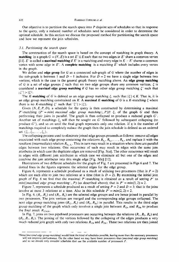
The construction of the search space is based on the concept of matching in graph theory. A matching in a graph G = (V, E) is a set E’ c E such that no two edges in E’ share a common vertex [I I]. E’ is called a maximal matching if E’ is a matching and every edge in E - E’ shares a common vertex with some edge in E’. A complete matching is a matching E’ which includes every vertex in the graph.

We define and edge group for G as a connected sub-graph of G where the number of edges in the sub-graph is between 1 and D - 1 inclusive. For D = 2 we have a single edge between two vertices; which is the case in the general graph theory matching above. An edge group matching of G is a set of edge groups 5 such that no two edge groups share any common vertices. c is considered a maximal edge group matching if G has no other edge group matching 5’ such that

15’1>151. The K-matching of G is defined as an edge group matching 5, such that 15 1 < K. That is, it is

an edge group matching constrained on K. A maximal K-matching of G is a K-matching r where there is no K-matching <’ such that 15’1 > ]r 1.

Given (IV, E, P, D), a schedule for the query is then constructed by determining a maximal P’-matching (P’ = min( Imaximal edge group matching 1, P))? l, of the graph G and then performing their joins in parallel. The graph is then collapsed to produce a reduced graph G’. Another set of matchings 5, will then be sought on G’ followed by subsequent collapsing (to produce G”), and so on until the final graph represents only one relation. If ye is the number of matchings required to completely reduce the graph then the join schedule is defined as an ordered

set Cl,, t2, . . .5,,>. The collapsing process used to eliminate joined edge groups proceeds as follows: remove all edges

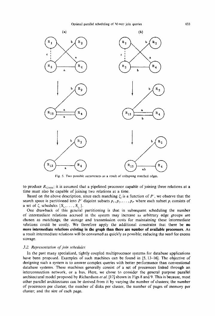
associated with each edge group containing the relations R,,, Rkz.. . . , Rk,, and replace it with the resultant (intermediate) relation R,,, k,. This in turn may result in a situation where there are parallel edges between two relations. One occurrence of such may result in edges with the same join attributes in which case the duplicate edges are removed [Fig. 5(a)]. The other occurrence will result in edges with different join attributes in which case we eliminate all but one of the edges and combine the join attributes into this single edge [Fig. 5(b)] [12].

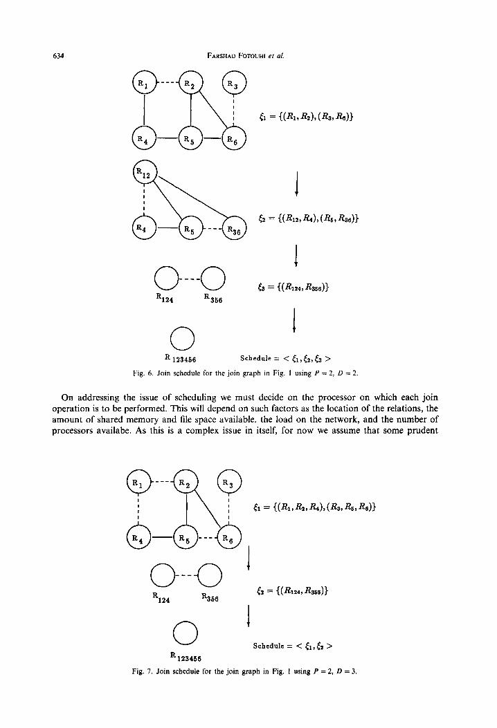
Illustrations of two different schedules for the graph of Fig. 1 are presented in Figs 6 and 7. The dotted lines in the figures represent the selected edges for the edge group.

Figure 6, represents a schedule produced as a result of utilizing two processors (that is P = 2) which are each able to join two relations at a time (that is D = 2). By examining the initial join graph of Fig. 6 we find that the maximal P/-matching is obtained as a result of setting P’ to min( Imaximal edge group matching 1, P) (as described above); that is P’ = min(3,2) = 2.

Figure 7, represents a schedule produced as a result of setting P = 2 and D = 3; that is the joins involve at most 3 relations at a time. Also in this schedule P’ = min(2, 2) = 2.

In Fig. 6, (R, , R2) and (R3, R6) are the selected edge groups and are hence joined in parallel by two processors. The join vertices are merged and the corresponding edge groups collapsed. The next edge group matching joins (R,,, R4) and (R,, R,,) in parallel. This results in the third edge group matching of the graph which only involves a single join between R,24 and Rjs6 to produce the final result R,13456.

In Fig. 7, joins on two pipelined processors are occurring between the relations (R, , R,, R4) and (R,, R,, R6). The joining of the vertices followed by the collapsing of the edges produces a very much reduced join graph with only two relations R,,, and R356. These two relations are then joined

Wince ~maximal edge group matching 1 would limit the kind of schedules possible, having more than the necessary processors will not improve performance. On the other hand we may have fewer processors than [maximal edge group marchingl and SO we should only consider schedules that use the available number of processors P.


Fig. 5. Two possible occurrences as a result of collapsing matched edges

to produce h.~ it is assumed that a pipelined processor capable of joining three relations at a time must also be capable of joining two relations at a time.

Based on the above description, since each matching & is a function of P’, we observe that the search space is partitioned into P’ disjoint subsets p, ,pZ, . . . ,py where each subset pi consists of a set of i, schedules {S,, , . . . , S,, }.

One drawback of this general partitioning is that in subsequent scheduling the number of intermediate relations accrued in the system may increase as arbitrary edge groups are chosen as matchings; the storage and transmission costs for maintaining these intermediate relations could be costly. We therefore apply the additional constraint that there be no more inte~m~iate relations existing in the graph than there are num~r of available processors. As a result intermediate relations will be consumed as quickly as possible; reducing the need for excess storage.

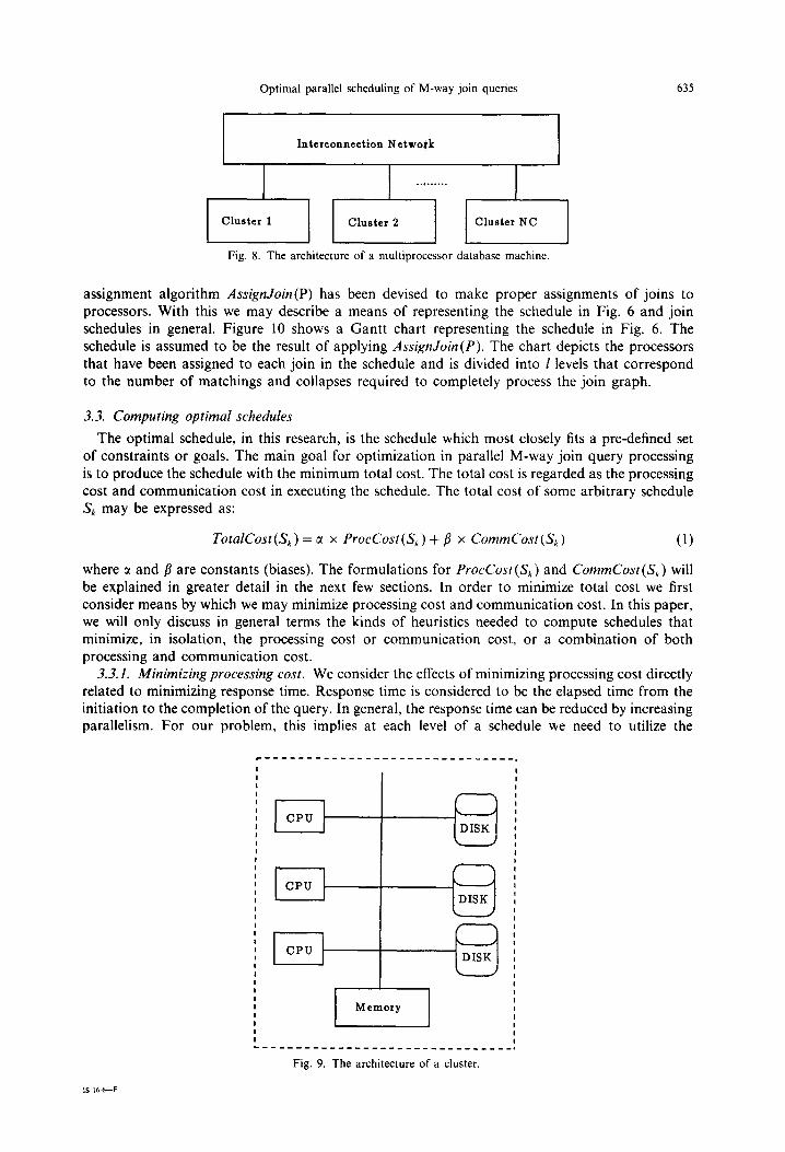
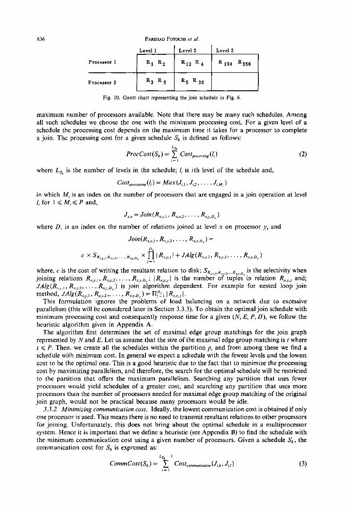
In the past many specialized, tightly coupled multiprocessor systems for database applications have been proposed. Examples of such machines can be found in [5,13-161. The objective of designing such a system is to answer complex queries with better performance than conventional database systems. These machines generally consist of a set of processors linked through an interconnection network, or a bus. Here, we chose to consider the general purpose parallel architectural model proposed by Richardson et al. [ 171 shown in Figs 8 and 9. This is because, most other parallel architectures can be derived from it by varying the number of clusters; the number of processors per cluster; the number of disks per cluster, the number of pages of memory per cluster; and the size of each page.

634 FARSHAD F0-rour-n et al.

O---O R124 R356

0 R 123456

t3 = ((%24, &56))

I Fig. 6. Join schedule for the join graph in Fig. I using P = 2, D = 2

On addressing the issue of scheduling we must decide on the processor on which each join operation is to be performed. This will depend on such factors as the location of the relations, the amount of shared memory and file space available, the load on the network, and the number of processors availabe. As this is a complex issue in itself, for now we assume that some prudent

t, = {(R~,Rz,%),(Rs,%,Rs)}

O---O R

+ < -((R 2- 124, 366 R )} 124 R366

0 R 123456

Schedule = < <I, (2 >

Fig. 7. Join schedule for the join graph in Fig. 1 using P = 2, D = 3.


Interconnection Netwofk

+++,

Fig. 8. The architecture of a multiprocessor database machine.

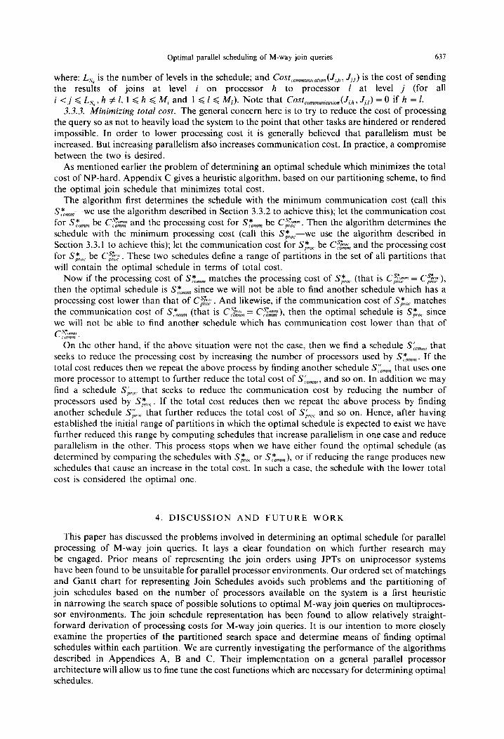
assignment algorithm AssignJoin has been devised to make proper assignments of joins to processors. With this we may describe a means of representing the schedule in Fig. 6 and join schedules in general. Figure 10 shows a Gantt chart representing the schedule in Fig. 6. The schedule is assumed to be the result of applying AssignJoin( The chart depicts the processors that have been assigned to each join in the schedule and is divided into 1 levels that correspond to the number of matchings and collapses required to completely process the join graph.

3.3. Computing optimal schedules

The optimal schedule, in this research, is the schedule which most closely fits a pre-defined set of constraints or goals. The main goal for optimization in parallel M-way join query processing is to produce the schedule with the minimum total cost. The total cost is regarded as the processing cost and communication cost in executing the schedule. The total cost of some arbitrary schedule S, may be expressed as:

TotalCost = c( x ProcCost(S,) + fl x CommCost(Sk) (1)

where c( and /? are constants (biases). The formulations for ProcCost(&) and CommCost(S,) will be explained in greater detail in the next few sections. In order to minimize total cost we first consider means by which we may minimize processing cost and communication cost. In this paper, we will only discuss in general terms the kinds of heuristics needed to compute schedules that minimize, in isolation, the processing cost or communication cost, or a combination of both processing and communication cost.

3.3.1. Minimizing processing cost. We consider the effects of minimizing processing cost directly related to minimizing response time. Response time is considered to be the elapsed time from the initiation to the completion of the query. In general, the response time can be reduced by increasing parallelism. For our problem, this implies at each level of a schedule we need to utilize the

L--_______________---------____.

Fig. 9. The architecture of a cluster.

636 FARSHAD FoT0u-n et al.

Fig. 10. Gantt chart representing the join schedule in Fig. 6.

maximum number of processors available. Note that there may be many such schedules. Among all such schedules we choose the one with the minimum processing cost. For a given level of a schedule the processing cost depends on the maximum time it takes for a processor to complete a join. The processing cost for a given schedule S, is defined as follows:

ProcCost(& 1 = 1 costprocessing (It 1 i=I

(2)

where L, is the number of levels in the schedule; li is ith level of the schedule and,

in which Mi is an index on the number of processors that are engaged in a join operation at level Z,for l<M,<Pand,

Jx9 = JOin U?,,, y R,y.2T . . . y R.v,y,D, )

where D, is an index on the number of relations joined at level x on processor y, and

where, c is the cost of writing the resultant relation to disk; SR,, ,,R, ,,2 ,., R. ,D, is the selectivity when . . . joining relations &,, , R.r,Jj,2, . . . : f.xg,D, ; 1 R,,y.j 1 is the number oi’ tup%s in relation R.,,j and;

J-WR,,:, 7 R.,?.,z 3 . . . 7 R,s,o,) is jam algorithm dependent. For example for nested loop join

method, J&(R,,y., , RXg,~~~ . . . , RX,y,D,v > = I'$, IR,,j I .

This formulation ignores the problems of load balancing on a network due to excessive parallelism (this will be considered later in Section 3.3.3). To obtain the optimal join schedule with minimum processing cost and consequently response time for a given (N, E, P, D), we follow the heuristic algorithm given in Appendix A.

The algorithm first determines the set of maximal edge group matchings for the join graph represented by N and E. Let us assume that the size of the maximal edge group matching is t where r < P. Then, we create all the schedules within the partition p, and from among these we find a schedule with minimum cost. In general we expect a schedule with the fewest levels and the lowest cost to be the optimal one. This is a good heuristic due to the fact that to minimize the processing cost by maximizing parallelism, and therefore, the search for the optimal schedule will be restricted to the partition that offers the maximum parallelism. Searching any partition that uses fewer processors would yield schedules of a greater cost, and searching any partition that uses more processors than the number of processors needed for maximal edge group matching of the original join graph, would not be practical because many processors would be idle.

3.3.2. Minimizing communication cost. Ideally, the lowest communication cost is obtained if only one processor is used. This means there is no need to transmit resultant relations to other processors for joining. Unfortunately, this does not bring about the optimal schedule in a multiprocessor system. Hence it is important that we define a heuristic (see Appendix B) to find the schedule with the minimum communication cost using a given number of processors. Given a schedule S,, the communication cost for S, is expressed as:

CommCoW$) = “‘5 ’ COS~communicorion (Jl.h 2 Jj.,> (3) i= I

Optimal parallel scheduling of M-way join queries 63-l

where: L,, is the number of levels in the schedule; and COS~~,,,,,,~,,,,,(J;,~, J,.,) is the cost of sending the results of joins at level i on processor h to processor 1 at level j (for all

i < j < L, , h # 1, 1 < h < M, and 1 < 1 < MI). Note that ~~~~~~~~~~~~~~~~~~~~~~~ J,,) = 0 if h = E. 3.3.3. Minimizing total cost. The general concern here is to try to reduce the cost of processing

the query so as not to heavily load the system to the point that other tasks are hindered or rendered

impossible. In order to lower processing cost it is generally believed that parallelism must be increased. But increasing parallelism also increases communication cost. In practice, a compromise between the two is desired.

As mentioned earlier the problem of determining an optimal schedule which minimizes the total cost of NP-hard. Appendix C gives a heuristic algorithm, based on our partitioning scheme, to find the optimal join schedule that minimizes total cost.

The algorithm first determines the schedule with the minimum communication cost (call this S,*,,,,,-we use the algorithm described in Section 3.3.2 to achieve this); let the communication cost for S,*,,, be C’fk; and the processing cost for SE,,,, be Ci:;ym. Then the algorithm determines the schedule with the minimum processing cost (call this S,*,,,.-we use the algorithm described in Section 3.3.1 to achieve this); let the communication cost for S&,. be Cs&, and the processing cost

for S&,, be C;j;y. These two schedules define a range of partitions in the set of all partitions that will contain the optimal schedule in terms of total cost.

Now if the processing cost of Sz,, matches the processing cost of S$,,. (that is Ci:rm = C&:), then the optimal schedule is S,*,,, since we will not be able to find another schedule which has a processing cost lower than that of C$g:. And likewise, if the communication cost of ST&, matches the communication cost of S$,,,,, (that is C:&m = Cs:omm ,,,,), then the optimal schedule is S$,,, since we will not be able to find another schedule which has communication cost lower than that of CZ.%;.

On the other hand, if the above situation were not the case, then we find a schedule S:,,, that seeks to reduce the processing cost by increasing the number of processors used by Sz,,,,,. If the total cost reduces then we repeat the above process by finding another schedule S:b,,,, that uses one more processor to attempt to further reduce the total cost of S:,,,,,, and so on. In addition we may find a schedule S;,,,‘ that seeks to reduce the communication cost by reducing the number of processors used by S,*,,,, . If the total cost reduces then we repeat the above process by finding another schedule Scion that further reduces the total cost of Sir,,, and so on. Hence, after having established the initial range of partitions in which the optimal schedule is expected to exist we have further reduced this range by computing schedules that increase parallelism in one case and reduce parallelism in the other. This process stops when we have either found the optimal schedule (as determined by comparing the schedules with S:&, or S,*,,,), or if reducing the range produces new schedules that cause an increase in the total cost. In such a case, the schedule with the lower total cost is considered the optimal one.

4. DISCUSSION AND FUTURE WORK

This paper has discussed the problems involved in determining an optimal schedule for parallel processing of M-way join queries. It lays a clear foundation on which further research may be engaged. Prior means of representing the join orders using JPTs on uniprocessor systems have been found to be unsuitable for parallel processor environments. Our ordered set of matchings and Gantt chart for representing Join Schedules avoids such problems and the partitioning of join schedules based on the number of processors available on the system is a first heuristic in narrowing the search space of possible solutions to optimal M-way join queries on multiprocessor environments. The join schedule representation has been found to allow relatively straight- forward derivation of processing costs for M-way join queries. It is our intention to more closely examine the properties of the partitioned search space and determine means of finding optimal schedules within each partition. We are currently investigating the performance of the algorithms described in Appendices A, B and C. Their implementation on a general parallel processor architecture will allow us to fine tune the cost functions which are necessary for determining optimal schedules.

638

PI

ti;

141

PI

PI

171

181

[91 WI

[I 11

WI

1131

1141 iI51 1161

P71

FARSHAD FOTC~UHI et al.

REFERENCES

D. H. Fishman, D. Beech, H. P. Cake, E. C. Chow, T. Connors, J. W. Davis, N. Derrett, C. G. Hoch, W. Kent, P. Lyngback, B. Nahbod, M. A. Neimat, T. A. Ryan and M. C. Shan. Iris: An object-oriented DBMS. ACM Trans. on Ofice Information Systems 5 (I), (1987). A. Swami and A. Gupta. Optimization of large join queries. Proc. of ACM SIGMOD pp. 48-69 (1988). D. Dewitt and R. Gerber. Multiprocessor hash-based join algorithms. Proc. 11th Int. Co& on VLDB pp. 151-164 (1985). P. Selinger, M. Astrahan, D. Chamberlin, R. Lorie and T. Price. Access path selection in a relational database management system. Proc. ACM SIGMOD pp. 23-34 (1979). P. Valduriez and G. Gardarin. Join and semijoin algorithms for a parallel multiprocessor database machine. ACM Trans. on Database Systems 9 (1), 133-161 (1984). E. Wong and K. Youssefi. Decomposition-A strategy for query processing. ACM Trans. on Database Systems 1 (3). 223-241 (1976). T. Ibaraki and T. Kameda. On the optimal nesting order for computing N-relational join. ACM Trans. on Database Systems 4 (3), 482-502 (1984). R. Krishnamurthy, H. Boral and C. Zaniolo. Optimization of nonrecursive queries. Proc. f21h Int. Conf. on VLDB pp. 128-137 (1986). A. Swami. Optimization of Large Join Queries. PhD dissertation, Stanford University, (1989). M. Stonebaker, E. Wong, P. Kreps and G. Held. The design and implementation of INGRES. ACM Trans. on Database Systems 1 (3), 198-222 (1976). M. Garey and D. Johnson. Computers and Intractability. A Guide to the theory of NP-Completeness. W. H. Freeman, San Francisco, CA (1979). Y. Zeng and F. Tong. A new approach to optimizing the multi-relation join. Proc. 6th Adoanced Database Symp. pp. 215-221 (1986). D. Bitton, H. Boral, D. Dewitt and W. Wilkinson. Parallel algorithms for the execution of relational databases operations. ACM Trans. on Database Systems 8 (3), 324-353 (1983). D. Hsiao. Advanced Database Machine Architecture. Prentice Hall, Englewood Cliffs, NJ (1986). E. Ozkarahan. Database Machines and Database Management. Prentice Hall, Englewood Cliffs, NJ (1986). D. Dewitt, R. Gerber, G. Graefe, M. Heytens, K. Kumar and M. Muralikrishna. GAMMA-A high performance dataflow database machine. Proc. 12th Int. Conf on VLDB pp. 228-237 (1986). J. Richardson, H. Lu and K. Mikkilineni. Design and evaluation of pipelined join algorithms. Proc. ACM SIGMOD pp. 399-409 (1987).

APPENDIX A

Minimum Processing Cost Algorithm

/* Algorithm for creating the minimum processing cost schedule for a given join graph */ CreateMinProcCostSchedule(N, E, P, D)

1 allScheds:={ }; minSched:=NIL; minCost:=INFINITY;

r:=SizeOfMaxEdgeGroupMatching(N, E); if (t > P) then {

r:=P;

!vhile (sched:=Generate A Schedule Not Already in allScheds given N, E, I, D) { allSchedsl=Union(allScheds, sched); cost:=ProcCost(sched); /* See Formulation 2 */ if (cost < mincost) then {

minCost:=cost; minSched:=sched;

1

II retum(minSched);

j

APPENDIX B

Minimum Communication Cost Algorithm

/* Algorithm for creating the minimum communication cost schedule for a given join graph */ /* This is essentially the same as the algorithm for computing the minimum */ /* processing cost schedule except that here the objective is to select the schedule */ /*with the minimum communication cost that utilizes P processors. */ CreateMinCommCostSchedule(N, E, P, D) { allScheds:={ }; minSched:=NIL; minCost:=INFINITY;

r:=SizeOlMaxEdgeGroupMatching(N, E); if ([ > P) then {

tg=P;

Optimal parallel scheduling of M-way join queries

while (sched:=Generate A Schedule Not Already in alkkheds given N, E, 1, D) { allScheds=Union(allScheds, sched); cost:=CommCost(sched); /* See formulation 3 */ if (cost < minCost) then {

minCost:=cost; minSched:=sched;

1) return(minSched);

1

639

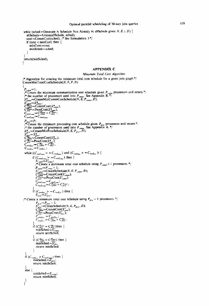
APPENDIX C

Minimum Total Cost Algorithm

/* Algorithm for creating the minimum total cost schedule for a given join graph */ CreateMinTotalCostSchedule(N, E, P, D) t

p?&itle the minimum communication cost schedule given P,.,, processors and return */ /* the number of processors used into P,.,,,,,,. See Appendix B. */ SZll”,~- -CreateMinCommCostSchedule(N, E, P,,,, D); s;M,,:=s:M,; cf$g;j =CommCost(S~~,); C~=ProcCost(S* ,); c mraCWVn 4y;; + 6%; CI”If&” ‘= C~“roiLW,“: Pp,“,.‘=P; /* Create the minimum processing cost schedule given P,,,w processors and return */ /* the number of processors used into PC,,,,,,,,,. See Appendix A. */ S$,,:=CreateMinProcSchedule(N, E, P,,,w, D); s:*,.1= S$, ; Cf? :=CommCost(S* ,)* CgJ=ProcCost(S*,O,.r ’ c~~;,$$~+&; C ,n,oi& I= C /“I+~, ;

while ((C,o,sl;,unW > = C,01nb.“,8 ) and (C,,,(,, ,,,) > = C,W,,~ )) {

if Gut_ 7 = Goru~._ “,,, 1 then {

s:.m,~=s:!“m,;

/* Create a minimum total cost schedule using P,,, + I processors. */ P,.,,I=P,.“,, + I ; S&,,,I=CreateSchedule(N, E, P,.,,, D); Cr$;:=CommCost(S:Omm); Cz-n-;=ProcCost(S&J; p,nr C,“,‘,l;.“,“,” ‘=Cmr.L” ; c ,“,“l;,“,,,“~=c~~ + c$?;

t if CC r 7 = C,,,,,,,,, 1 then {

s;;;Yzs;,,w ;

/* Create a minimum total cost schedule using P,,,,,<- I processors. */ P ,=p - 1; S~K:=d’;eMateSchedule(N, E, P,,,w, D); CFk>=CommCost(S”,,,.); C~;:=ProcCost(S~,,X~; c,O,+~~ = c,od,,,,, ;

:=cr ’ + c;jy

/f ;:z:: = Ci;)&.n { ’ mi%hedlz?&,, return minSched;

1 if (CF&, = C,,,, OMIT) then {

min!khed~=S~,, return mindched;

I ’ if (C,,,,,,,, 7 C,orrrl;,,n 1 then i mmSched:=Si,,, ; return minSched;

I else (

minScheda=S:.,,,,,,; return minSched;

Optimal parallel scheduling of M-way join queries

Documents