Optimal output-transitions for linear systems

Available online at www.sciencedirect.com

Automatica 39 (2003) 181–192

www.elsevier.com/locate/automatica

Optimal output-transitions for linear systems�

Hector Perez, Santosh Devasia∗

Mechanical Engineering Department, University of Washington, Box 352600, Seattle, WA 98115-2600, USA

Received 3 April 2001; received in revised form 6 April 2002; accepted 26 August 2002

Abstract

This article addresses the optimal (minimum-input-energy) output-transition problem for linear systems. The goal is to transfer theoutput from an initial value y(t) = y (for all time t6 ti) to a /nal output value y(t) = 0y (for all time t¿ tf ). Previous methods solvethis output-transition problem by transforming it into a state-transition problem; the initial and /nal states (x(ti); x(tf ), respectively) arechosen and a minimum-energy state-to-state transition problem is solved. However, the choice of the initial and /nal states can be adhoc and the resulting output-transition cost (input energy) may not be minimal. The contribution of this article is the solution of theoptimal output-transition problem. An example system with elastic dynamics is studied to illustrate the proposed method. Simulationresults are presented that show substantial reduction of transition costs with the use of the proposed method when compared to the useof minimum-energy state-to-state transitions.? 2002 Elsevier Science Ltd. All rights reserved.

Keywords: Optimal control; Output transition; Minimum energy; Inversion; Precision positioning; Vibration compensation

1. Introduction

Changing the output of a system from one value toanother (i.e. output transition) is a fundamental controlproblem. Formally, the problem studied in this article isto transfer the system output, with minimum input energy,from an initial value y(t) = y (for all time t6 ti) to a /naloutput value y(t) = 0y (for all time t¿ tf ) as shown in Fig.1. Such output-transition problems arise in a wide range ofapplications, for example, in the positioning of 9exiblestructures which include: (I) large-scale light-weight (andtherefore, 9exible) space manipulators and antennae(Farrenkopf, 1979; Singhose, Banerjee, & Seering, 1997;Wie, Sinha, & Liu, 1993); (II) medium-scale read-writeheads of disk drives (Ho, 1997; Miu & Bhat, 1991); and(III) relatively small-scale piezo-based nano-positioners(Bleuler, Clavel, Breguet, Langeu, & Peanette, 2000; Croft,Shedd, & Devasia, 2001). During output transitions, theelastic dynamics of these structures can lead to residual

� This paper was not presented at any IFAC meeting. This paper wasrecommended for publication in revised form by Associate Editor KenkoUchida under the direction of the Editor Tamer Basar.

∗ Corresponding author.E-mail addresses: hectorr [email protected] (H. Perez), devasia@

u.washington.edu (S. Devasia).

vibrations after the completion of a positioning maneuver,which results in loss of positioning precision. Such vibra-tions in the output could take a prohibitively long time toreduce to an acceptable level. Therefore, procedures thatminimize (or remove) residual output-vibrations are neededto achieve acceptable transitions in these systems; such anapproach to output transitions is studied in this article.The contribution of this article is the solution of the

minimal-input-energy, output-transition problem. Previousmethods solve the output-transition problem by transform-ing it into a state-transition problem. In such methods, theinitial and /nal states (x(ti) = x, x(tf ) = 0x, respectively)are chosen, and an optimal state-transition problem (fromx(ti) to x(tf )) is solved (Lewis & Syrmos, 1995). For exam-ple, the initial and /nal states can be chosen as equilibriumstates of the system at the initiation (t = ti) and completion(t = tf ) of the output transition. This choice, of initial and/nal states, enables the output to be maintained at the de-sired value y(t)= 0y without residual vibrations (for all timet¿ tf ). In 9exible structures such equilibrium states corre-spond to rigid-body con/gurations of the structure. How-ever, the choice of equilibrium states as the initial and /nalstates may not be optimal. On the other hand, an arbitrarychoice of the initial and /nal states is also not acceptablebecause it can lead to transient errors, for example, after the

0005-1098/03/$ - see front matter ? 2002 Elsevier Science Ltd. All rights reserved.PII: S0005 -1098(02)00240 -6

mailto:[email protected]



182 H. Perez, S. Devasia / Automatica 39 (2003) 181–192

Final Output Value

Initial Output Value

Time

Output

minimize ∫ − ∞

∞uTRu dty(t) = y for all t ≤ ti

ti tf

y

y

≥y(t) = y for all t tf

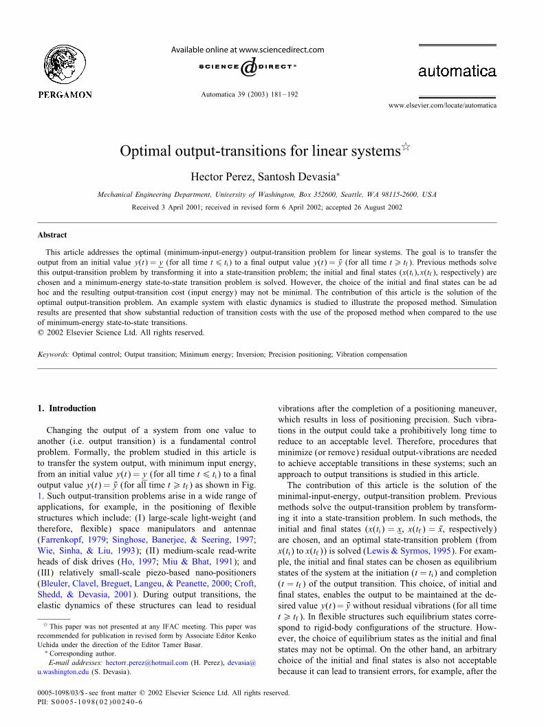
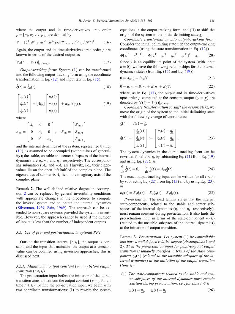
Fig. 1. The output-transition problem.

completion of the output transition. The novelty of the pro-posed approach is that it quanti/es the possible choices inthe initial and /nal states and then optimally chooses themto minimize the output-transition cost.The proposed approach uses pre- and post-actuation in-

puts to reduce the transition cost (i.e., input energy) withoutchanging the output-transition time (Ttran = tf − ti). For ex-ample, consider the transfer of a disk-drive read-write headfrom one track of a disk to another track. Pre-actuation canbe used before the initiation of the output transition to setup the optimal initial condition without changing the outputposition, i.e., maintain the read-write head over the initialtrack (y=y for time t6 ti). Similarly, post-actuation can beused after the completion of the output transition to main-tain the read-write head over the /nal track (y= 0y for timet¿ tf ). Because the output is precisely controlled during thepre- and post-actuation phase, read and write operations canstill be performed during the pre- and post-actuation. Thus,the eHective seek time (i.e., the time interval (ti; tf ) duringwhich read and write operations cannot be performed) is noteHected by the use of the pre- and post-actuation.In contrast to the output-transition problem, the state-

transition problem is well understood. Note that a control-lable linear system can be transferred from any initial stateto any /nal state; there are multiple input trajectories thatcould achieve such a state transition. For example, if theboundary conditions (initial state x(ti) = x and /nal statex(tf ) = 0x) are prescribed, then a control input can be cho-sen using standard optimal control approaches (see, e.g.,Lewis & Syrmos, 1995) to minimize (I) the time takento achieve the state transition (i.e., minimum time prob-lems), or (II) the input energy needed to achieve the tran-sition. Such state-transition approaches have been used toachieve zero-residual-vibration output transitions in 9exiblestructures. For example, the input-shaping scheme (e.g., inSinghose et al., 1997; Pao & Lau, 2000) /nds an input suchthat the output and a suitable number of its time derivativesare zero after the transition. Necessary and suJcient con-ditions for an input to achieve such zero-residual-vibrationstate-transitions were characterized in the Laplace domainin Bhat and Miu (1990). The central idea in these techniquesis to avoid vibrations by completing the maneuver with a

/nal state (x(tf )= 0x at time tf ) that is a rigid-body con/gura-tion with zero elastic-deformations. Thus, these techniquesplace a constraint on the state at the completion of the outputtransition; in contrast, the proposed approach does not con-strain the /nal state. Rather the proposed output-transitionapproach only requires that the /nal output 0y be achievedat time tf—the output is then maintained at the /nal valuey = 0y using inversion-based post-actuation input for timet ¡ tf . Similarly, the proposed approach does not constrainthe state at the initiation of the output transition (x(ti)), anda pre-actuation input for time t ¡ ti is used to maintain theoutput value y=y before the initiation of the output transi-tion (Devasia, Chen, & Paden, 1996). The additional free-dom in the choice of the boundary states (x(ti) and x(tf ))is then exploited to optimally reduce the output-transitioncost. It is noted that the use of pre-actuation requires thatthe output-transition’s start time ti be known in advance. Ifthe start time ti is not known in advance then the proposedapproach can be modi/ed to only use post-actuation withoutpre-actuation (see Remark 5).The optimal output-transition problem was posed pre-

viously in Piazzi & Visioli (2000, 2001), in which aninversion-based approach was used to plan an output tran-sition. However, these results require the user to specify(a priory) the set of acceptable output trajectories duringthe transition (using polynomials); the method to choosethe output trajectory is ad hoc. Similar pre-speci/cationof a desired output trajectory was also used by Dowdand Thanos (2000) to achieve smooth transitions betweenoutput-trajectory segments in industrial positioning sys-tems. In contrast, we do not require the pre-speci/cationof the output trajectory; rather, the best output trajectory isobtained as the result of the proposed optimization proce-dure. We do however, use the stable inversion approach (asin Piazzi & Visioli (2000, 2001)) to /nd the pre-actuation(t ¡ ti) inputs that maintain output tracking y = y be-fore the initiation of the output transition, and similarlyto /nd post-actuation (t ¿ tf ) inputs to maintain the out-put at 0y. The inversion-based approach, used to /nd pre-and post-actuation inputs, is then integrated with standardoptimal control approaches during the output transition (be-tween times ti and tf ) to solve the optimal output-transitionproblem.The paper is organized as follows. In Section 2, the

point-to-point output-transition (PPT) problem is formu-lated. Two approaches are proposed: (I) using standardstate-to-state transition approach; and (II) integrating thestate-to-state transition approach with an inversion-basedpre- and post-actuation approach, which yields the optimalsolution to the PPT problem (presented in Section 3). Theproposed method is illustrated using an example systemwith elastic dynamics in Section 4. Simulation results showsubstantial reduction of transition costs with the use ofthe proposed method when compared to the use of previ-ous techniques that are based on state-to-state transitions.Conclusions are in Section 5.

H. Perez, S. Devasia / Automatica 39 (2003) 181–192 183

2. Problem formulation

We begin by formulating the PPT problem.

2.1. PPT problem

Consider a square (same number of inputs as outputs),linear, time-invariant system described by

x(t) = Ax(t) + Bu(t); y(t) = Cx(t); (1)

where x(t)∈Rn is the state, u(t)∈Rp is the input andy(t)∈Rp is the output. A direct feedforward term Du(t)can be included in the output equation; however, it is omit-ted to simplify the presentation. Furthermore, let x and 0x beequilibrium points of the system (also referred to as delim-iting states), and let the corresponding outputs be y and 0yrespectively, i.e.,

De�nition 1. Delimiting states for transition.x = Ax = 0; y = Cx;

0x = A 0x = 0; 0y = C 0x:(2)

The output-transition problem is formally stated next.

De�nition 2. PPT problem. Given the delimiting states andthe transition time interval [ti; tf ], /nd a bounded input-statetrajectory [uH (·); xref (·)] such that the following three re-quirements are met:

(I) The system equations are satis/ed for all time(−∞¡t¡∞)xref (t) = Axref (t) + BuH (t); yref (t) = Cxref (t):

(II) The output transitions from y to 0y in the time interval[ti; tf ]. The output is maintained at the desired value beforeand after the output transition

yref (t) = y for all t6 ti;

yref (t) = 0y for all t¿ tf :

(III) The system state approaches the delimiting states astime goes to (plus or minus) in/nity,

xref (t)→ x as t → −∞;

xref (t)→ 0x as t → ∞:

Remark 1. Although the goal is to transfer the system be-tween the delimiting states x and 0x, the critical issue is tochange the output from y to 0y in a speci/ed transition time,Ttran=tf−ti. Therefore, the states at the beginning and end ofoutput transitions, xref (ti) and xref (tf ), need not be the delim-iting states, x and 0x. Pre- and post-actuation inputs, appliedoutside of the transition interval, [ti; tf ], could be used totransfer the state xref to the delimiting states. Such changesin state xref outside of the transition interval are acceptableas long as the output is maintained at the desired value.

2.2. Approach 1: state-to-state transition

One approach to achieve the output transition is to transferthe system between the delimiting states, i.e., from x(ti)= xto x(tf )= 0x within the transition time. It is noted that the /naldelimiting state is an equilibrium point; therefore, the sys-tem state can be maintained at that value without changingthe output. (For 9exible structures, these delimiting statescould correspond to rigid body con/gurations; therefore,there are no residual vibrations.) If the system is control-lable, then there is an input that can achieve the desiredstate-to-state output transition; however, this input is notunique. In the following, we require that the input chosen forthe state-to-state transition (SST) should minimize the in-put energy required for the transition. This minimal-energySST problem can be posed and solved using standard linearquadratic optimal (LQ) control theory (see, e.g., Lewis &Syrmos, 1995).

Assumption 1. In the following, we assume that System (1)is controllable.

De�nition 3. Minimal-energy SST problem. Find abounded input-state trajectory [uH (·); xref (·)] that transfersSystem (1) from an initial state x(ti) to a /nal state x(tf )and minimizes the following cost function

Jsst(ti; tf ; x(ti); x(tf ); u) =∫ tf

ti

uTRu dt; (3)

where R is a positive-de/nite symmetric matrix.

De�nition 4. Final-state di5erence. If no input is appliedduring the time interval [ti; tf ], then the state of the systemat time tf will be eA(tf−ti)x(ti). The diHerence between thisno-applied-input state and the desired state x(tf ) at time tf , isreferred to as the /nal-state diHerence, and can be written as

d(ti; tf ) = x(tf )− eA(tf−ti)x(ti): (4)

Lemma 1. Solution to minimal-energy SST problem.Given the boundary states x(ti) and x(tf ), the input usst(·)that minimizes the cost function Jsst is given by

usst(t) = R−1BTeAT(tf−t)G−1

(ti ;tf )d(ti; tf ); (5)

where G(ti ;tf ) is the invertible controllability grammiangiven by

G(ti ;tf ) =∫ tf

ti

eA(tf−�)BR−1BTeAT(tf−�) d�: (6)

The transition cost when using the minimum-energy SSTinput (5) is given by

J ∗sst(ti; tf ; x(ti); x(tf )) = d(ti; tf )

TG−1(ti ;tf )

d(ti; tf ): (7)

Proof. See, for example, (Lewis & Syrmos, 1995,p. 165).


An approach to achieve point-to-point output-transition(PPT) is to use the minimal energy solution to the SST prob-lem, where the initial and /nal states for this SST problemare the initial and /nal delimiting states, respectively. Thisis stated formally in the next lemma.

Lemma 2. Standard PPT. A solution to the PPT problemis to use the minimal energy solution to the SST problem(Lemma 1) with the state at the initiation of the outputtransition chosen as the initial delimiting state (x(ti) = x),and similarly with the state at the completion of the outputtransition chosen as the 8nal delimiting state (x(tf ) = 0x).The input uH = usppt is given by

usppt(t) = R−1BTeAT(tf−t)G−1

(ti ;tf )d(ti; tf ) if ti6 t6 tf

= 0 otherwise; (8)

where d(ti; tf ) = [ 0x− eA(tf−ti)x]. The reference state trajec-tory xref = xsppt is given by

xsppt(t) = x if t ¡ ti

= eA(t−ti)x +∫ t

ti

{eA(t−�)Busppt(�)} d�

if ti6 t6 tf

= 0x if t ¿ tf (9)

and the cost Jsppt of using input usppt is given by

Jsppt(ti; tf ) = d(ti; tf )TG−1(ti ;tf )

d(ti; tf ): (10)

Proof. From Lemma 1, the state is transferred from x to 0x.Conditions 2 and 3 for PPT (see De/nition 2) are satis/edsince x and 0x are delimiting states (see De/nition 1).

The solution to the PPT problem achieved using theminimum-energy solution to the SST problem is referred toas the standard approach to the PPT problem (or standardPPT, in short). It is noted that the standard PPT does not usepre- or post-actuation. In the following, we explore the useof pre- and post-actuation to further reduce the transitioncost.

2.3. Approach 2: optimal output transition

The choice of the states [x(ti); x(tf )], at the initiation t= tiand completion t = tf of the output transition, need not be/xed a priori as the delimiting states (x; 0x) (as was done inthe standard PPT approach). In the following, the states atthe initiation and completion of the output transition are con-sidered as variables in the control-design, and are optimized.This optimal point-to-point output-transition (optimal PPT)problem, is stated next.

De�nition 5. Optimal PPT problem. Find a boundedinput-state trajectory [uH (·); xref (·)] that solves the output-

transition problem (see De/nition 2), and minimizes thefollowing cost function

Jppt(ti; tf ; u) =∫ ∞

−∞uTRu dt; (11)

where R is a positive-de/nite symmetric matrix (as inEq. (3)).

3. Solution to the optimal PPT problem

The optimal point-to-point output-transition (optimalPPT) problem is solved in this section. This is done inthree steps: (I) transforming the system into output-trackingform; (II) /nding the input needed before the initiation ofoutput transition (pre-actuation) and after the completion ofthe output transition (post-actuation); and (III) integratingthe pre- and post-actuation with the minimal energy SSTapproach to /nd the solution to the optimal PPT problem.

3.1. Output-tracking form

In the PPT problem, the output has to be maintainedconstant outside the transition interval—this can be doneusing inversion-based approaches. We begin by rewritingthe system equations in the output-tracking form (see, e.g.,Isidori, 1989, Chapter 4; Sastry, 1999, Chapter 9), under thefollowing assumption.

Assumption 2. System (1) has a well-de/ned relative de-gree � (e.g., see Sastry, 1999), where � := [�1; �2; : : : ; �p].

Output-tracking form. Under Assumption 2, there exists(I) a coordinate transformation, �, and (II) an input law thattransforms the system into the output-tracking form (see,e.g., Isidori, 1989; Sastry, 1999).Coordinate transformation: The system state x is trans-

formed into the following new coordinates:

�[ �T Ts Tu Tc ]T = x; (12)

where the output and its time-derivatives upto order �−1 :=[�1 − 1; �2 − 1; : : : ; �p − 1] are denoted by�= [y1; y 1; : : : ; d�1−1y1=dt�1−1; y2; y 2; : : : ; d�2−1y2=dt�2−1;

: : : ; yp; y p; : : : ; d�p−1yp=dt�p−1]T (13)

and s; u ; c represent the stable, unstable, and centersubspaces of the internal dynamics , respectively. Further-more, the output and its time-derivatives upto order �−1 areknown if the desired output is speci/ed; this known term isde/ned as

�d(t) = �(t)|y(·)=yd(·): (14)

Input law: The input law needed for the transformationhas the following general form

uH (t) = Bs s(t) + Bu u(t) + Bc c(t) + B�Y(t); (15)


where the output and its time-derivatives upto order�= [�1; �2; : : : ; �p] are denoted by

Y= [�T; d�1y1=dt�1 ; d�2y2=dt�2 ; : : : ; d�pyp=dt�p ]T: (16)

Again, the output and its time-derivatives upto order � areknown in terms of the desired output as

Yd(t) =Y(t)|y(t)=yd : (17)

Output-tracking form: System (1) can be transformedinto the following output-tracking form using the coordinatetransformation in Eq. (12) and input law in Eq. (15):

�(t) = �d(t); (18)

s(t)

u(t)

c(t)

= [Aint]

s(t)

u(t)

c(t)

+ BintYd(t); (19)

where

Aint =

As 0 0

0 Au 0

0 0 Ac

; Bint =

Bint;s

Bint;u

Bint;c

and the internal dynamics of the system, represented by Eq.(19), is assumed to be decoupled (without loss of general-ity); the stable, unstable and center subspaces of the internaldynamics are s; u, and c, respectively. The correspond-ing submatrices As, and −Au are Hurwitz, i.e., their eigen-values lie on the open left half of the complex plane. Theeigenvalues of submatrix Ac lie on the imaginary axis of thecomplex plane.

Remark 2. The well-de/ned relative degree in Assump-tion 2 can be replaced by general invertibility conditionswith appropriate changes in the procedures to computethe inverse system and to obtain the internal dynamics(Silverman, 1969; Sain, 1969). The approach can be ex-tended to non-square systems provided the system is invert-ible. However, the approach cannot be used if the numberof inputs is less than the number of independent outputs.

3.2. Use of pre- and post-actuation in optimal PPT

Outside the transition interval [ti; tf ], the output is con-stant, and the input that maintains the output at a constantvalue can be obtained using inversion approaches; this isdiscussed next.

3.2.1. Maintaining output constant (y = y) before outputtransition (t6 ti)The pre-actuation input before the initiation of the output

transition aims to maintain the output constant (y=y for alltime t6 ti). To /nd the pre-actuation input, we begin withtwo coordinate transformations: (I) to rewrite the system

equations in the output-tracking form; and (II) to shift theorigin of the system to the initial delimiting state x.Coordinate transformation into output-tracking form:

Consider the initial delimiting state x in the output-trackingcoordinates (using the state transformation in Eq. (12))

�[ �T T ]T := �[ �T sT uT cT ]T = x: (20)

Since x is an equilibrium point of the system (with inputu= 0), we have the following relationships for the internaldynamics states (from Eq. (15) and Eq. (19))

0 = Aint + BintY (21)

0 = Bs s + Bu u + Bc c + B�Y; (22)

where, as in Eq. (17), the output and its time-derivativesupto order � computed at the constant output (y = y) aredenoted by Y(t) =Y(t)|y(t)=y.Coordinate transformation to shift the origin: Next, we

move the origin of the system to the initial delimiting statewith the following change of coordinates:

�(t) := �(t)− �;

(t) :=

s(t)

u(t)

c(t)

:=

s(t)− s

u(t)− u

c(t)− c

: (23)

The system dynamics in the output-tracking form can berewritten for all t ¡ ti, by subtracting Eq. (21) from Eq. (19)and using Eq. (23), asddt

�(t) = 0;ddt

(t) = Aint (t): (24)

The exact output tracking input can be written for all t ¡ ti,by subtracting Eq. (22) from Eq. (15) and by using Eq. (23),as

uH (t) = Bs s(t) + Bu u(t) + Bc c(t): (25)

Pre-actuation: The next lemma states that the internalstate-components, related to the stable and center sub-spaces of the internal dynamics ( s and c, respectively),must remain constant during pre-actuation. It also /nds thepre-actuation input in terms of the state-component u(ti)(related to the unstable subspace of the internal dynamics)at the initiation of output transition.

Lemma 3. Pre-actuation. Let system (1) be controllableand have a well de8ned relative degree (Assumptions 1 and2). Then the pre-actuation input for point-to-point outputtransition is uniquely speci8ed in terms of the state com-ponent u(ti) (related to the unstable subspace of the in-ternal dynamics) at the initiation of the output transition(time ti).

(1) The state-components related to the stable and cen-ter subspaces of the internal dynamics must remainconstant during pre-actuation, i.e., for time t6 ti

s(t) = s; c(t) = c: (26)


(2) The exact-output maintaining, pre-actuation input fortime t ¡ ti is given by

upre(t) = Bu[eAu(t−ti ) u(ti)]

= Bu[eAu(t−ti)( u(ti)− u)]: (27)

Proof. The internal dynamics Eq. (24) is autonomous, andan explicit solution to the internal dynamics (for time t ¡ ti)can be found as (t)=e−Aint (ti−t) (ti). Then, the requirementthat the system state should tend to the delimiting state x astime t goes to −∞ (see requirement 3, in De/nition 2) canbe expressed in terms of the above solution to the internaldynamics as

0 = limt→−∞ s(t) = lim

t→−∞ e−As(ti−t) s(ti);

0 = limt→−∞ u(t) = lim

t→−∞ e−Au(ti−t) u(ti);

0 = limt→−∞ c(t) = lim

t→−∞ e−Ac(ti−t) c(ti):

(28)

From this equation, we obtain the following constraint onthe state at the initiation of the output transition at time t= ti

s(ti) = 0; c(ti) = 0 (29)

because submatrices −As and −Ac are not Hurwitz. For anyother values of the stable subspace of the internal dynam-ics s(ti) and the center subspace of the internal dynamics c(ti), the system will not go to the delimiting state x ast → −∞. The /rst statement of the lemma (see Eq. (26))follows from Eqs. (23) and (29). While the state compo-nents of the stable and center subspaces of the internaldynamics are constrained, there are no such restrictions onthe choice of the state component of the unstable subspace, u(ti). The delimiting state can be achieved for any choiceof the unstable subspace of the internal dynamics u(ti)because submatrix −Au is Hurwitz. The second statementof the Lemma (Eq. (27)) follows by substituting Eq. (29)into Eq. (25) and then using the de/nition of u inEq. (23).

Note that the pre-actuation input is completely speci-/ed in terms of the unstable component u(ti) of the inter-nal dynamics at the initiation of the desired output transi-tion. Therefore, the cost of the pre-actuation input can bequanti/ed in terms of this component as shown in the nextLemma.

Lemma 4. Pre-actuation cost. For a speci8ed unstablesubspace of the internal dynamics u(ti) the cost of thepre-actuation input is equal to

Jpre( u(ti))

:=∫ ti

−∞uTpre(t)Rupre(t) dt

= Tu (ti)Wpre u(ti)− 2 Tu (ti)Wpre u + uTWpre u ; (30)

where

Wpre =∫ ∞

0e−ATu �BTuRBue

−Au� d� (31)

can be found by solving the Lyapunov equation

WpreAu + ATuWpre = BTuRBu : (32)

Proof. From Eqs. (27) and (30)

Jpre( u(ti))

= uT

ti∫−∞

eATu (t−ti)BTuRBue

Au(t−ti) dt

u

= uT[ ∫ ∞

0e−ATu �BTuRBue

−Au�d�] u

by setting − �= (t − ti)

=[ u(ti)− u]TWpre[ u(ti)− u]:

Since submatrix −Au is Hurwitz, Wpre in the above equa-tion can be found as the unique, symmetric solution tothe following Lyapunov equation (see, e.g., Chen, 1999,Theorem 5.6, Chapter 6), Wpre(−Au) + (−Au)TWpre =−BTuRBu, which completes the proof.

3.2.2. Maintaining output constant (y = 0y) afteroutput-transition (t¿ tf )The post-actuation after the completion of the output tran-

sition aims to maintain the output constant (y(t) = 0y for alltime t¿ tf ). As in the pre-actuation case, we begin with twocoordinate transformations: (I) to rewrite the system equa-tions in the output-tracking form; and (II) to shift the originof the system to the /nal delimiting state 0x.Coordinate transformation and shift of origin to 0x; Con-

sider the /nal delimiting state 0x in the output-tracking coor-dinates (using the state transformation in Eq. (12))

�[ 0�T sT uT cT ]T = 0x: (33)

Furthermore, let the origin of the system be moved to the/nal delimiting state 0x

0�(t) := �(t)− 0�; s(t) := s(t)− s;

u(t) := u(t)− u ; c(t) := c(t)− c;(34)

where a bar above the variables indicates that the variablesare related to the post-actuation phase of the PPT.Post-actuation input and cost: The next lemma states

that the state-components related to the unstable and centersubspaces of the internal dynamics ( u and c, respectively)must remain constant during post-actuation. It also obtainsthe post-actuation input upost in terms of the state-component s(tf ), which is related to the stable subspace of the internaldynamics at the completion of output transition. The resultsof this next lemma are then used to quantify the cost of usingthe post-actuation input.


Lemma 5. Post-actuation. Let system (1) be controllableand have a well de8ned relative degree (Assumptions 1and 2). Then the post-actuation input for point-to-pointoutput transition is uniquely speci8ed in terms of the statecomponent s(tf ), which is related to the stable subspace ofthe internal dynamics at the completion of output transition(time tf ).

(1) The state-components related to the unstable and cen-ter subspaces of the internal dynamics must remainconstant during post-actuation, i.e., for all time t¿ tf u(t) = u and c(t) = c,

(2) the exact-output maintaining, post-actuation input fortime t ¿ tf is given by

upost(t) = uH (t) = Bs[eAs(t−tf ) s(tf )]

= Bs[eAs(t−tf )( s(tf )− s)]: (35)

Proof. This proof is similar to the proof of Lemma 3, andso this proof is omitted.

Lemma 6. Post-actuation cost. For a speci8ed stablesubspace of the internal dynamics s(tf ), the cost of thepost-actuation input is equal to

Jpost( s(tf ))

:=∫ ∞

tf

uTpost(t)Rupost(t) dt

= Ts (tf )Wpost s(tf )

− 2 Ts (tf )Wpost s + sTWpost s (36)

where

Wpost =∫ ∞

0eA

Ts �BTs RBse

As� d� (37)

is the solution to the Lyapunov equation

WpostAs + ATsWpost =−BTs RBs: (38)

Proof. This proof is similar to the proof of Lemma 4, andis omitted.

3.3. Optimal PPT

Lemmas 3 and 5 imply that the only freedom in the statex(ti), at the initiation of PPT, is in the choice of the unstablecomponent u(ti) of the internal dynamics. Similarly, theonly freedom in the state x(tf ), at the completion of PPT,is in the choice of the stable component s(tf ) of the inter-nal dynamics. Therefore, a particular choice of these statecomponent variables, u(ti) and s(tf ), completely speci/esthe boundary states [x(ti); x(tf )] at the initiation t = ti andcompletion t = tf of the PPT problem.

De�nition 6. Boundary conditions #. Components of thestate, at the initiation and completion of output transition,that can be varied while achieving the desired output tran-sition (i.e., solving the PPT problem) are

# := [ Ts (tf ) Tu (ti)]T: (39)

Remark 3. Standard PPT boundary conditions. Theboundary conditions # are constrained to be the delim-iting states when using the standard PPT solution to theoutput-transition problem, i.e. # = # := [ 0 Ts Tu ]

T.

Remark 4. Optimal PPT boundary conditions. The bound-ary conditions # are not constrained to be # (as in Remark3) in the optimal PPT approach; they are chosen to optimizethe energy used for the output transition.

3.3.1. Minimum-energy PPT for a speci8ed #Once this minimum-energy PPT is found for given

boundary conditions #, then the optimal PPT can be foundby optimizing the boundary conditions. For a set of pre-scribed boundary conditions #, the energy needed for thePPT can be found by adding (I) the minimum energy neededduring the output-transition time-period [ti; tf ] and (II) theenergy needed outside the output-transition time-period(i.e., t ¡ ti and t ¿ tf ). We begin by /nding the minimumenergy needed during the output-transition time-period.Minimum energy during output transition: Lemmas 3

and 5 imply that the only freedom in the choice of state x(ti)at the initiation of output transition and in the choice of statex(tf ) at the completion of the output transition are in thechoice of boundary conditions #. The choice of boundaryconditions # speci/es the pre- and post-actuation inputs(and associated costs); however, it does not specify the inputduring the output-transition interval [ti; tf ]. The input energyneeded during the output-transition interval can be optimizedby using minimum-energy SST technique (see Lemma 1)with the initial and /nal states chosen as

x(ti) = �[�T sT u(ti)T cT]T;

:= [�� |� s |� u |� c ][�T sT u(ti)T cT]T

(40)

x(tf ) = �[ 0�T s(tf )T uT cT]T:

The associated minimum input-energy J ∗sst(ti; tf ; #) during

the output transition time-period can be written in terms ofthe boundary condition # as (using Eqs. (4) and (7))

J ∗sst(ti; tf ; #) = d#(ti; tf )TG−1

(ti ;tf )d#(ti; tf ); (41)

where d#(ti; tf ) is the /nal-state diHerence d(ti; tf ) rewrittenin terms of the boundary conditions # as (using De/nition4 and Eq. (40))

d#(ti; tf ) = H1f + H2#; (42)


where

H1 := [�� |� u |� c | −W� | −W s | −W c ]

H2 : =[� s | −W u ]

[W� |W s |W u |W c ] := eA(tf−ti)[�� |� s |� u |� c ]

f := [ 0� 0 u 0 c � s c ]T:

The minimum input-energy J ∗sst(ti; tf ; #) during the output

transition time-period can be rewritten as (using Eqs. (41)and (42))

J ∗sst(ti; tf ; #)

=(H1f + H2#)TG−1(ti ;tf )

(H1f + H2#)

=#THT2 G

−1(ti ;tf )

H2# + 2#THT2 G

−1(ti ;tf )

H1f

+fTHT1 G

−1(ti ;tf )

H1f (43)

Lemma 7. Minimum-energy PPT for prescribed boundaryconditions#. For a given choice of the boundary conditions# (as de8ned in Eq. (39)), the minimum energy needed toachieve the point-to-point output transition is quadratic in# and has the form

Jppt(ti; tf ; #) =#T%# − 2#Tb+ c: (44)

Proof. The total cost Jppt(ti; tf ; #) over all time t ∈(−∞;∞), for minimal energy PPT with a speci/edchoice of boundary conditions #, can then be obtainedby adding the cost J ∗

sst(ti; tf ; #) during output transitionto the pre-actuation cost Jpre( u(ti)) and post-actuationcost Jpost( s(tf )). The lemma follows by substituting forJpre( u(ti)), Jpost( s(tf )), and J ∗

sst(ti; tf ; #), from Eqs. (30),(36), and (43), respectively, and setting

% :=

[Wpost 0

0 Wpre

]+ HT

2 G−1(ti ;tf )

H2; (45)

b :=

[Wpost s

Wpre u

]− HT

2 G−1(ti ;tf )

H1f;

c := sTWpost s + uTWpre u + fTHT1 G

−1(ti ;tf )

H1f:

3.3.2. Solution to the optimal PPT problemOptimal values for the boundary conditions # are found

in the following theorem, which also obtains the input thatsolves the optimal PPT problem.

Theorem 1. Optimal PPT. Let system (1) be controllableand have a well-de8ned relative degree (Assumptions 1 and2). Then the optimal PPT problem always has a solutionas described in the following three statements.

(1) The PPT cost function (Eq. (11)) is minimized bythe following choice of boundary conditions # = #∗ =[( ∗s )

T ( ∗u)T]T given by

#∗ = %−1b if % is invertible;

#∗ = %†b otherwise; (46)

where %† is the pseudo (generalized) inverse of % (e.g., seeOrtega, 1987 for the de8nition of the generalized inverse).(II) The optimal input uH =u∗ppt can include pre-actuation

(t ¡ ti) and post-actuation (t ¿ tf ), and is given by

u∗ppt(t) = Bu[eAu(t−ti)( ∗u − u)] if t ¡ ti;

= R−1BTeAT(tf−t)G−1

(ti ;tf )d#∗(ti; tf )

if ti6 t6 tf , where d#∗(ti; tf ) is obtained by setting#=#∗

in Eq. (42) and

u∗ppt(t) = Bs[eAs(t−tf )( ∗s − s)] if t ¿ tf :

(III) The corresponding reference state trajectory xref =xppt is given by

xppt(t)

=�[�T sT [e−Au(ti−t)( ∗u − u) + u]T cT]T

if t ¡ ti

= eA(t−ti)x(ti) +∫ t

ti

{eA(t−�)Bu∗ppt(�)} d�

if ti6 t6 tf

=�[ 0�T [e−As(tf−t)( ∗s − s) + s]T uT cT]T

if tf ¡t:

Proof. From Lemma 7, the cost function (Eq. (11)) can bewritten as a quadratic form in terms of boundary conditions# as shown in Eq. (44). Since the cost function (Eq. (11))is quadratic in the input, it has a lower bound (zero!). Theexistence of the lower bound implies that the optimizationproblem always has at least one solution (e.g., see Ortega,1987, Theorem 4.2.1, in Chapter 4). Similarly, the /rst partof the Theorem follows from optimization of quadratic forms(e.g., see Ortega, 1987, Theorem 4.2.1, Chapter 4). Thesecond part of the theorem follows from Lemmas 1, 3 and5 (Eqs. (5), (27) and (35)). The third part of the Theoremfollows by integrating system equation (1) with the optimalPPT input.

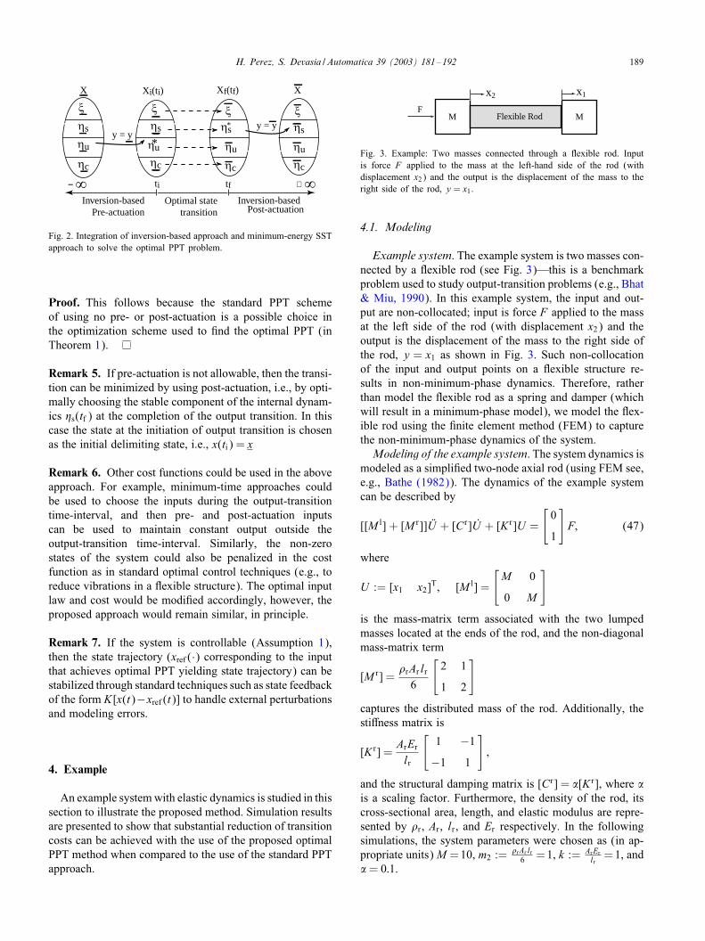
Thus, the optimal PPT integrates inversion-based pre- andpost-actuation with minimum energy SST to solve the opti-mal output-transition problem—this is represented in Fig. 2.

Corollary 1. The cost of the optimal PPT is less thanor equal to the cost of the standard PPT (de8nedin Lemma 2).


Xi(ti)

ξ ξ ξ ξ

Xf(tf)

ηu* ηu

ηsηsηs

ηuηcηc ηc

*

ηc

ηs

ηuy = y

Post-actuation

X X

Inversion-basedPre-actuation

Inversion-based

y = y

Optimal statetransition

ti tf− ∞ + ∞

Fig. 2. Integration of inversion-based approach and minimum-energy SSTapproach to solve the optimal PPT problem.

Proof. This follows because the standard PPT schemeof using no pre- or post-actuation is a possible choice inthe optimization scheme used to /nd the optimal PPT (inTheorem 1).

Remark 5. If pre-actuation is not allowable, then the transi-tion can be minimized by using post-actuation, i.e., by opti-mally choosing the stable component of the internal dynam-ics s(tf ) at the completion of the output transition. In thiscase the state at the initiation of output transition is chosenas the initial delimiting state, i.e., x(ti) = x

Remark 6. Other cost functions could be used in the aboveapproach. For example, minimum-time approaches couldbe used to choose the inputs during the output-transitiontime-interval, and then pre- and post-actuation inputscan be used to maintain constant output outside theoutput-transition time-interval. Similarly, the non-zerostates of the system could also be penalized in the costfunction as in standard optimal control techniques (e.g., toreduce vibrations in a 9exible structure). The optimal inputlaw and cost would be modi/ed accordingly, however, theproposed approach would remain similar, in principle.

Remark 7. If the system is controllable (Assumption 1),then the state trajectory (xref (·) corresponding to the inputthat achieves optimal PPT yielding state trajectory) can bestabilized through standard techniques such as state feedbackof the form K[x(t)−xref (t)] to handle external perturbationsand modeling errors.

4. Example

An example systemwith elastic dynamics is studied in thissection to illustrate the proposed method. Simulation resultsare presented to show that substantial reduction of transitioncosts can be achieved with the use of the proposed optimalPPT method when compared to the use of the standard PPTapproach.

x1x2

M MF

Flexible Rod

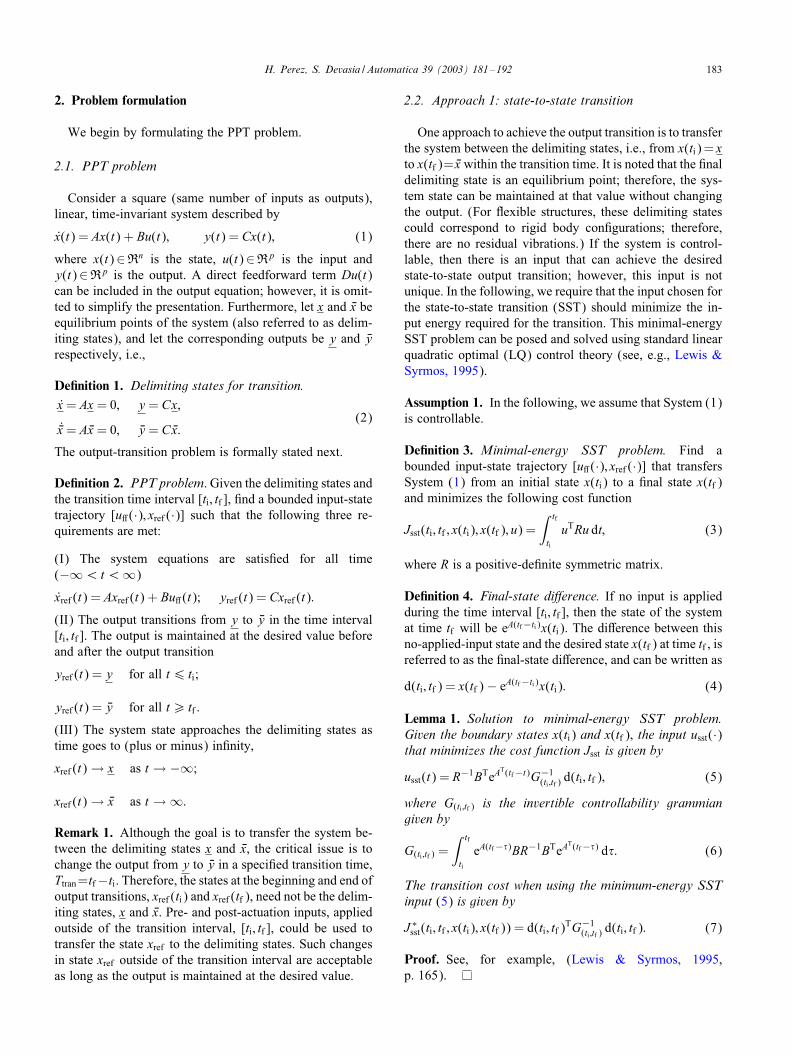
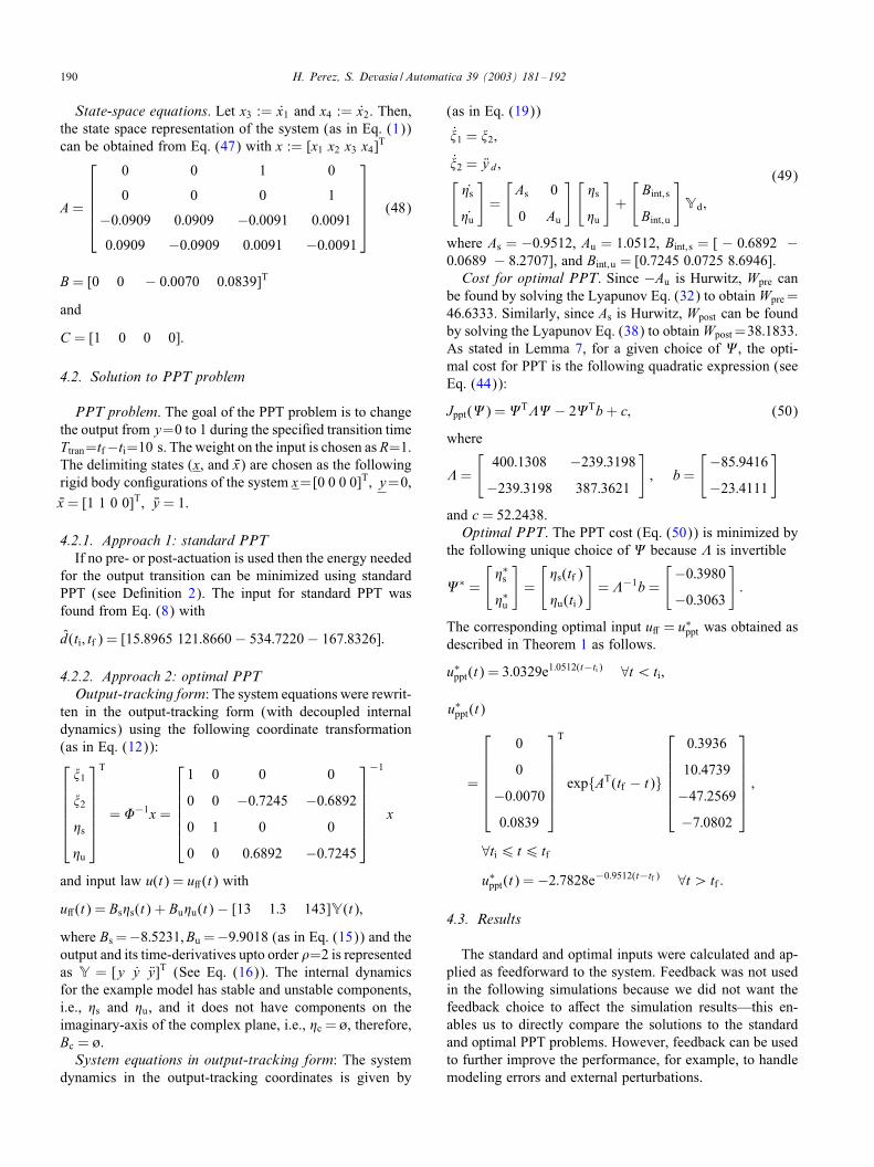
Fig. 3. Example: Two masses connected through a 9exible rod. Inputis force F applied to the mass at the left-hand side of the rod (withdisplacement x2) and the output is the displacement of the mass to theright side of the rod, y = x1.

4.1. Modeling

Example system. The example system is two masses con-nected by a 9exible rod (see Fig. 3)—this is a benchmarkproblem used to study output-transition problems (e.g., Bhat& Miu, 1990). In this example system, the input and out-put are non-collocated; input is force F applied to the massat the left side of the rod (with displacement x2) and theoutput is the displacement of the mass to the right side ofthe rod, y = x1 as shown in Fig. 3. Such non-collocationof the input and output points on a 9exible structure re-sults in non-minimum-phase dynamics. Therefore, ratherthan model the 9exible rod as a spring and damper (whichwill result in a minimum-phase model), we model the 9ex-ible rod using the /nite element method (FEM) to capturethe non-minimum-phase dynamics of the system.Modeling of the example system. The system dynamics is

modeled as a simpli/ed two-node axial rod (using FEM see,e.g., Bathe (1982)). The dynamics of the example systemcan be described by

[[M l] + [M r]] VU + [Cr]U + [K r]U =

[0

1

]F; (47)

where

U := [x1 x2]T; [M l] =

[M 0

0 M

]

is the mass-matrix term associated with the two lumpedmasses located at the ends of the rod, and the non-diagonalmass-matrix term

[M r] =�rArlr6

[2 1

1 2

]

captures the distributed mass of the rod. Additionally, thestiHness matrix is

[K r] =ArErlr

[1 −1−1 1

];

and the structural damping matrix is [Cr] = /[K r], where /is a scaling factor. Furthermore, the density of the rod, itscross-sectional area, length, and elastic modulus are repre-sented by �r , Ar , lr , and Er respectively. In the followingsimulations, the system parameters were chosen as (in ap-propriate units) M =10, m2 :=

�rArlr6 =1, k := ArEr

lr=1, and

/= 0:1.


State-space equations. Let x3 := x1 and x4 := x2. Then,the state space representation of the system (as in Eq. (1))can be obtained from Eq. (47) with x := [x1 x2 x3 x4]T

A=

0 0 1 0

0 0 0 1

−0:0909 0:0909 −0:0091 0:0091

0:0909 −0:0909 0:0091 −0:0091

(48)

B= [0 0 − 0:0070 0:0839]T

and

C = [1 0 0 0]:

4.2. Solution to PPT problem

PPT problem. The goal of the PPT problem is to changethe output from y=0 to 1 during the speci/ed transition timeTtran=tf−ti=10 s. The weight on the input is chosen as R=1.The delimiting states (x, and 0x) are chosen as the followingrigid body con/gurations of the system x=[0 0 0 0]T; y=0,0x = [1 1 0 0]T; 0y = 1.

4.2.1. Approach 1: standard PPTIf no pre- or post-actuation is used then the energy needed

for the output transition can be minimized using standardPPT (see De/nition 2). The input for standard PPT wasfound from Eq. (8) with

d(ti; tf ) = [15:8965 121:8660− 534:7220− 167:8326]:

4.2.2. Approach 2: optimal PPTOutput-tracking form: The system equations were rewrit-

ten in the output-tracking form (with decoupled internaldynamics) using the following coordinate transformation(as in Eq. (12)):

�1

�2

s

u

T

= �−1x =

1 0 0 0

0 0 −0:7245 −0:68920 1 0 0

0 0 0:6892 −0:7245

−1

x

and input law u(t) = uH (t) with

uH (t) = Bs s(t) + Bu u(t)− [13 1:3 143]Y(t);

where Bs =−8:5231; Bu =−9:9018 (as in Eq. (15)) and theoutput and its time-derivatives upto order �=2 is representedas Y = [y y Vy]T (See Eq. (16)). The internal dynamicsfor the example model has stable and unstable components,i.e., s and u, and it does not have components on theimaginary-axis of the complex plane, i.e., c = H, therefore,Bc = H.System equations in output-tracking form: The system

dynamics in the output-tracking coordinates is given by

(as in Eq. (19))

�1 = �2;

�2 = Vyd;[ s

u

]=

[As 0

0 Au

][ s

u

]+

[Bint;s

Bint;u

]Yd ;

(49)

where As = −0:9512, Au = 1:0512, Bint;s = [ − 0:6892 −0:0689 − 8:2707], and Bint;u = [0:7245 0:0725 8:6946].Cost for optimal PPT. Since −Au is Hurwitz, Wpre can

be found by solving the Lyapunov Eq. (32) to obtainWpre =46:6333. Similarly, since As is Hurwitz, Wpost can be foundby solving the Lyapunov Eq. (38) to obtainWpost =38:1833.As stated in Lemma 7, for a given choice of #, the opti-mal cost for PPT is the following quadratic expression (seeEq. (44)):

Jppt(#) =#T%# − 2#Tb+ c; (50)

where

%=

[400:1308 −239:3198−239:3198 387:3621

]; b=

[−85:9416−23:4111

]

and c = 52:2438.Optimal PPT. The PPT cost (Eq. (50)) is minimized by

the following unique choice of # because % is invertible

#∗ =

[ ∗s

∗u

]=

[ s(tf )

u(ti)

]= %−1b=

[−0:3980−0:3063

]:

The corresponding optimal input uH = u∗ppt was obtained asdescribed in Theorem 1 as follows.

u∗ppt(t) = 3:0329e1:0512(t−ti) ∀t ¡ ti;

u∗ppt(t)

=

0

0

−0:00700:0839

T

exp{AT(tf − t)}

0:3936

10:4739

−47:2569−7:0802

;

∀ti6 t6 tf

u∗ppt(t) =−2:7828e−0:9512(t−tf ) ∀t ¿ tf :

4.3. Results

The standard and optimal inputs were calculated and ap-plied as feedforward to the system. Feedback was not usedin the following simulations because we did not want thefeedback choice to aHect the simulation results—this en-ables us to directly compare the solutions to the standardand optimal PPT problems. However, feedback can be usedto further improve the performance, for example, to handlemodeling errors and external perturbations.


0 5 10 15 20 25 30-0.5

0

0.5

1.0

1.5

0 5 10 15 20 25 30 -10

0

10

Inpu

t u

Out

put

y

time [sec]

time [sec]

ti tf

Fig. 4. Comparison of output and input time-trajectories for standard PPT(dotted line) and optimal PPT (solid line)—the optimal PPT input haspre- and post-actuation, however, the time for output transition is thesame (10 s) for both methods. The output transition is initiated at timet = ti = 10 s and completed at time t = tf = 20 s.

It is noted that the feedforward inputs are pre-computedusing the simulation model; therefore, the actual systemstates are not needed in this implementation. Furthermore,the optimal PPT input (found through the inversion method)is applied before the initiation of the output transition; thus,the optimal input is non-causal in this sense. However, theinversion-based pre-actuation input can be computed and ap-plied online if preview information of the output transitionis available (see, Zou & Devasia, 1999 for preview-basedcomputation of inverse inputs). In the simulations, the in-puts were computed oXine and pre- and post-actuation timeswere chosen as 10 s.

Remark 8. From Theorem 1, it can be seen that thepre-actuation input decays exponentially to zero as timet → −∞. The decay rate is proportional to the mini-mum distance Drhp of the right half-plane zeros of thesystem (i.e., poles of Au) from the imaginary axis ofthe complex plane. As this distance, increases, a smallerpreactuation-time can be chosen to achieve the desired ac-curacy in output-tracking—typically, a preactuation timeof 10=Drhp is suJcient. Similarly, the post-actuation timeneeded depends on the minimum distance Dlhp of the lefthalf-plane zeros of the system (i.e., poles of As) fromthe imaginary axis of the complex plane—typically, apost-actuation time of 10=Dlhp is suJcient.

Simulation results: Simulation results, when inputs forthe standard PPT and the optimal PPT were applied to theexample system, are presented in Figs. 4–6. Fig. 4 comparesthe inputs used in the standard and optimal PPT, and Fig. 5compares the evolution of the states. Note that the input isonly applied during the output-transition period, i.e., pre- andpost-actuation are not used for the standard PPT; however,both pre- and post-actuation are used in the optimal PPT.

0 10 20 30

0

1

5

0 10 20 30

0

0 10 20 30

0

1

1.5

0 10 20 30

0

1

0 10 20 30-1

0

0 10 20 30-1

0

0.5

-0.5

0.5

0.5

-0.5

0.5

0.5

-0.5

-0.5

-0.1

0.1

0.3y = ξ1 y = ξ2

ηs ηu

−0.5

ti

time [sec] time [sec]

y = x1 y = x3

x2 x4

.

ti

ti

tf

tf

tf

ti

ti

ti

tf

tf

tf

Fig. 5. Comparison of state time-trajectories for standard PPT (dottedline) and optimal PPT (solid line) with input weight R = 1. The stableand unstable components of the internal state ( s, and u) are shown inthe bottom plots.

8 10 12 14 1601

2

3

4

5

6

8 10 12 14 160

10

20

30

40

Tot

al c

ost

8 10 12 14 1605

10

15

20

30

8 100

200

400

Tot

al c

ost

Standard PPT Optimal PPT

Transition time [sec] Transition time [sec]

max

. in

put m

agni

tude

137.8

10.34

10.88

3.03

max

. in

put m

agni

tude

25

800

600

12 14 16

Fig. 6. Comparison of costs and maximum input magnitudes for standardPPT (dotted line) and optimal PPT (solid line) when the transition timeTtran = tf − ti is varied. It is noted that the cost for optimal PPT is alwaysless than the cost for standard PPT.

Fig. 6 shows the optimal cost and maximum magnitudesof inputs found for standard and optimal PPT for varioustransition times.Comparison of standard and optimal PPT: The simu-

lation results in Fig. 6 show that the cost for optimal PPTinput is always lower than the cost for standard PPT input(i.e., without pre- or post-actuation) for diHerent transitiontimes (as expected, see Corollary 1). For this example, withan output-transition time of 10 s and R = 1, the cost forthe standard PPT (de/ned in Eq. (7)) is J ∗

sst(ti; tf ) = 137:8.The cost of optimal PPT input is 10.88 (for the same 10 soutput-transition time), which is 12.7 times smaller thanthe cost of standard PPT input. Fig. 6 also shows that themagnitudes of the inputs used in optimal PPT are also sub-stantially lower than the magnitudes of inputs needed for


the standard PPT, especially as the transition time becomesmaller. For the 10 s output-transition time, the maximummagnitude of the standard PPT input is 10.34. The max-imum amplitude of the input with optimal PPT is 3.03,which is 3.4 times smaller than the maximum amplitude forthe input needed for the standard PPT (for the same 10 soutput-transition time). Note that both methods result in zeroresidual vibrations in the output, however the optimal PPTachieves it with lower input cost by exploiting the use ofpre- and post-actuation.

5. Conclusions

A technique to achieve optimal point-to-point output tran-sition was presented. Freedom in the choice of the internaldynamics was exploited using pre- and post-actuation in-puts (using inversion schemes) to optimize the input energyneeded to achieve this output transition. The method wasapplied to a simpli/ed 9exible-structure model and simula-tion results were presented to illustrate the advantages of thetechnique over standard state-to-state optimal control tech-niques.

Acknowledgements

Financial support from NASA Ames Research CenterGrant NAG 2-1450 and Grant NSF-CMS 0196214 is grate-fully acknowledged.

References

Bathe, K. J. (1982). Finite element procedures in engineering analysis.Englewood CliHs, NJ: Prentice-Hall.

Bhat, S. P., & Miu, D. K. (1990). Precise point-to-point positioningcontrol of 9exible structures. ASME Journal of Dynamics System,Measurements, Control, 112, 667–674.

Bleuler, H., Clavel, R., Breguet, J. M., Langen, H., & Pernette, E.(2000). Issues in precision motion control and microhandling. InIEEE proceedings of the International conference on robotics andautomation. San Francisco, CA, (pp. 959–964).

Chen, C. T. (1999). Linear system theory and design (3rd ed.). NewYork: Oxford University Press.

Croft, D., Shedd, G., & Devasia, S. (2001). Creep, hysteresis, andvibration compensation for piezoactuators: Atomic force microscopyapplication. ASME Journal of Dynamics System, Measurements,Control, 123(1), 35–43.

Devasia, S., Chen, D., & Paden, B. (1996). Nonlinear inversion-basedoutput tracking. IEEE Transactions on Automic Control, 41(7), 930–942.

Dowd, A. V., & Thanos, M. D. (2000). Vector motion processing usingspectral windows. IEEE Control Systems Magazine, 20(5), 8–19.

Farrenkopf, R. L. (1979). Optimal open-loop maneuver pro/les for9exible spacecraft. Journal of Guidance Control and Dynamics, 20(2),291–297.

Ho, H. T. (1997). Fast servo bang-bang seek control. IEEE Transactionson Magnetics, 33(6), 4522–4527.

Isidori, A. (1989). Nonlinear control systems: An introduction (3rd ed.).New York: Springer.

Lewis, F. L., & Syrmos, V. L. (1995). Optimal control. New York, NY10158–0012: Wiley, Third Avenue.

Miu, D. K., & Bhat, S. P. (1991). Minimum power and minimum jerkposition control and its applications in computer disk drives. IEEETransactions on Magnetics, 27(6), 4471–4475.

Ortega, J. M. (1987). Matrix theory. New York: Plenum Press.Pao, L. Y., & Lau, M. A. (2000). Robust input shaper control designfor parameter variations in 9exible structures. ASME Journal ofDynamics System, Measurements, Control, 122(1), 63–70.

Piazzi, A., & Visioli, A. (2000). Minimum-time system-inversion-basedmotion planning for residual vibration reduction. IEEE/ASMETransactions on Mechatronics, 5(1), 12–22.

Piazzi, A., & Visioli, A. (2001). Optimal inversion-based control for theset-point regulation of nonminimum-phase uncertain scalar systems.IEEE Transactions on Automatic Control, 46(10) 1654–1659.

Sain, M. K., & Massey, J. L. (1969). Invertibility of linear time-invariantdynamical systems. IEEE Transactions on Automatic Control, 14,141–149.

Sastry, S. (1999). Nonlinear systems. Analysis, stability and control.New York: Springer.

Silverman, L. M. (1969). Inversion of multivariable linear systems. IEEETransactions on Automatic Control, 14(3), 270–276.

Singhose, W. E., Banerjee, A. K., & Seering, W. P. (1997). Slewing9exible spacecraft with de9ection-limiting input shaping. Journal ofGuidance Control and Dynamics, 20(2), 291–297.

Wie, B., Sinha, R., & Liu, Q. (1993). Robust time-optimal control ofuncertain structural dynamic systems. Journal of Guidance Controland Dynamics, 16(5), 980–983.

Zou, Q., & Devasia, S. (1999). Preview-based stable-inversion foroutput tracking. ASME Journal of Dynamics Systems,Measurements,Control, 121(4), 625–630.

Hector Perez received the bachelor de-gree in Electrical Engineering in 1983 andthe M.S degree in System Engineering in1991 from the Universidad Nacional deColombia, and Ph.D. degree in MechanicalEngineering from the University of Utah in2002.He is a Research Professor in the ElectronicEngineering Department, at the Universi-dad Ponti/cia Bolivariana, Bucaramanga,Colombia, since June 2002. Previously,he had worked as a consultant developing

technical software for Electrical and Petroleum industries. His currentresearch interests include inversion-based control theory, high-precisionpositioning systems, optimal control theory, and the application of controltechnology in the Colombian industry. He is a member of ASME, andIEEE.

Santosh Devasia received the B.Tech.(Hons.) from the Indian Institute of Tech-nology, Kharagpur, India, in 1988, and theM.S. and Ph.D. degrees in mechanical en-gineering from the University of Californiaat Santa Barbara in 1990 and 1993 respec-tively.He is an Associate Professor in the Me-chanical Engineering Department, at theUniversity of Washington, Seattle (since2000). Previously, he had taught atthe Mechanical Engineering Department,

University of Utah, Salt Lake City. His current research interests includeinversion-based control theory, high-precision positioning systems fornanotechnology and biomedical applications, and the control of complexdistributed systems such as Air TraJc Management. These projects arefunded through, NSF and NASA grants. He is a member of AIAA,ASME, and IEEE.

Optimal output-transitions for linear systems

Documents