Optimal multiplier load flow method using concavity theory

Applied Mathematics and Computation 245 (2014) 487–503

Contents lists available at ScienceDirect

Applied Mathematics and Computation

journal homepage: www.elsevier .com/ locate/amc

Optimal multiplier load flow method using concavity theory

http://dx.doi.org/10.1016/j.amc.2014.07.1130096-3003/� 2014 Elsevier Inc. All rights reserved.

⇑ Corresponding author at: Department of Electrical Engineering, Faculty of Engineering, University of Malaya, 50603, Malaysia.

A. Shahriari a,b,⇑, H. Mokhlis a,b, A.H.A. Bakar b, H.A. Illias a,b

a Department of Electrical Engineering, Faculty of Engineering, University of Malaya, 50603, Malaysiab University of Malaya Power Energy Dedicated Advanced Centre (UMPEDAC), Level 4, Wisma R&D UM, University of Malaya, 59990 Kuala Lumpur, Malaysia

a r t i c l e i n f o

Keywords:Optimal multiplier load flow methodIll-conditioned systemLow voltage solutionMaximum loading point

a b s t r a c t

This paper utilises concavity properties in the optimal multiplier load flow method(OMLFM) to find the most suitable low voltage solution (LVS) for the systems having multi-ple LVS at the maximum loading point. In the previous method, the calculation of the opti-mal multiplier is based on only one remaining low voltage solution at the vicinity ofvoltage collapse point. However, this does not provide the best convergence for multi-low voltage solutions at the maximum loading point. Therefore, in this paper, concavityproperties of the cost function in OMLFM are presented as the indicator to find the mostsuitable optimal multiplier in order to determine the most suitable low voltage solutionsat the maximum loading point. The proposed method uses polar coordinate system insteadof the rectangular coordinate system, which simplifies the task further and by keeping PVtype buses. The polar coordinate in this method is based on the second order load flowequation in order to reduce the calculation time. The proposed method has been validatedby the results obtained from the tests on the IEEE 57, 118 and 300-bus systems for well-conditioned systems and at the maximum loading point.

� 2014 Elsevier Inc. All rights reserved.

1. Introduction

Load flow analysis is important in providing the initial conditions for many power system analyses such as transient sta-bility, fault analyses and contingency analysis. Load flow analysis is used intensively in the planning of a new power systemnetwork or expansion of an existing power system network. In the past, a large number of solution methods have been intro-duced to improve various power flow problems, especially to improve the convergence speed for well-conditioned powersystem [1–4]. For ill-conditioned systems, researchers are more concerned on the divergence of power flow equations in con-ventional methods and systems operating in infeasible zone [5–7]. A power system becomes ill-conditioned due to the highR/X ratio of transmission lines or the loading of the system is approaching the maximum loading point (MLP). The stability ofa power system is greatly affected in ill-conditioned system [8–10].

In load flow analysis, the load flow equations consist of an algebraic set of nonlinear quadratic equations, which have sev-eral solutions. However, at least one of the solutions is the operating point of interest for the system, which corresponds tostable equilibrium points for well-conditioned systems [1,11,12]. The load flow solutions are commonly found using thestandard Newton–Raphson load flow (SNRLF) method [13,14], where flat initial guesses are made (all bus voltages of PQ-type bus equal to 1 and their voltage angles equal to zero). Although the solutions using the SNRLF method exist, stable equi-librium solutions may not be found. This is due to the region of the solutions is far from the operation point and due to theapplication of numerical method in the SNRLF method [12,14–16].

Nomenclature

D vector of independent variablesL vector of dependent variablesS vector function of load flowx coefficient related to dependent and independent variablesG function of nonlinear inequality constraintsW function of nonlinear equality constraintsU control parameter for independent variablesk convergence correction multiplier (optimal multiplier)MLFS multiple load flow solutionsHVS high voltage solutionOEF optimisation energy functionEFPS energy function of a power systemMLP maximum loading pointSNRLF standard Newton–Raphson load flowOMLFM optimal multiplier load flow method

488 A. Shahriari et al. / Applied Mathematics and Computation 245 (2014) 487–503

For power systems which several solutions exist, the solutions can be divided into two types; low voltage solutions(LVS) and high voltage solutions (HVS). LVS is referred to unstable equilibriums, which present a low-voltage profile insome buses while the operating point of interest is referred as HVS [16]. The number of LVS decreases when the loadof the system is increased in a way that at the voltage collapse point neighbourhood, only one LVS remains. When theload of the system is increased further, the HVS can intersect with the one remaining LVS [12,17]. This LVS is called asthe critical LVS in a saddle-node bifurcation point and it disappears when the load is kept increasing, where the load flowsolutions become unavailable [18,19]. The load that corresponds to this critical LVS is known as the maximum loadingpoint (MLP) [16].

There are two main approaches of finding the LVS; the curve tracing method (CTM) or path following method [8,19,20]and the state space search method (SSSM) [13,21,22]. The CTM uses a trajectory of the load increase direction to detect theMLP. This method is considered robust and powerful in detecting LVS. However, the disadvantage of CTM is for convergence,it needs a large number of iterations and previous information of the direction of the load demand increment. However, thedetermination of LVS using SSSM does not require many iterations and any previous information of the load increase direc-tion. The SSSM searches for LVS in a chosen direction of the state space and then, the LVS is determined using an interactiveload flow solver method [6,23].

The work in this paper focuses on ill-conditioned power flow problems. For ill-conditioned power systems, the multipleload flow solutions can be determined using the optimal multiplier load flow method (OMLFM) [13]. This method applies theoptimal multiplier based on SSSM concept to the SNRLF method. It was found that the solution never diverges but convergesin a way that the value of the cost function always reduces. This cost function is known as the energy function of power sys-tem (EFPS) and its derivative function with respect to the accelerator multiplier is called the optimisation energy function(OEF) [13,21]. When there are more than one real solutions of the optimal multiplier, the lowest optimal multiplier isselected, which is commonly used in most of the literature [17,24]. The optimal multiplier is then used to update the esti-mation of bus voltage vectors.

The optimal multiplier concept has also been utilised to estimate multiple load flow solutions by using three optimalmultipliers in [21]. This method was used to find a pair of multiple load flow solutions that are closely located to each other,which is related with voltage instabilities in power systems. It was discovered that the convergent characteristics of loadflow calculation by the SNRLF method in rectangular coordinates has a unique linearity. They tend to converge straighttoward a pair of multiple solutions when they are closely located to each other. Therefore, Iba et al. has proposed a newmethod for solving a pair of near solutions in power systems. The proposed method was able to obtain those solutions byone or two times of conventional load flow calculations with additional processes. The proposed method can also confirmthe existence of other solutions near a conventional solution.

Overbye in his publication has shown that the optimal multiplier from the OMLFM approaches zero at the maximumloading point due to the singularity of Jacobian matrix [15]. To overcome this problem, Overbye has selected the optimalmultiplier closest to one, or the maximum optimal multiplier to find the LVS in a feasible boundary zone of the systemoperating point. This selection is based on the remaining LVS at the vicinity of the voltage collapse point neighbourhood.When the load is increased further, the smallest and largest roots of OEF move towards each other and meet at the localmaximum point, which is at the middle root of the EFPS [14,23]. This case is referred to the system having multiple LVS atthe MLP [16]. However, the direction of OEF roots movement may lead the OMLFM to blind search in detecting the LVS.This has resulted in there is no guarantee that using the optimal multiplier closest to one leads to an optimum point ofEFPS [16,21,25].

A. Shahriari et al. / Applied Mathematics and Computation 245 (2014) 487–503 489

In this paper, concavity properties of the cost function using OMLFM are presented as the indicator to find the most suit-able optimal multiplier in order to determine the most suitable low voltage solutions at the maximum loading point. If theselection of optimal multiplier is inappropriate, the most suitable LVS for the system having multi-LVS will not be obtained[26,27]. Therefore, the fixed point theory concept is used in the proposed method to find the stationary point of EFPS. Usingthis method, the obtained optimal multipliers at the MLP can verify the roots of EFPS to be the safe operating point frominfeasibility boundary zone. Also, all low voltage solutions in the trajectory of an increasing load demand can be obtained.The proposed method uses the second order load flow equation in polar coordinate to find the optimal multiplier [3]. Thepolar coordinate of OMLFM is fast and has a robust execution than the rectangular coordinate, by keeping PV type buses[22,24,28].

In section II of this paper, the theoretical and mathematical backgrounds of optimal multiplier in finding the multiple loadflow solutions are detailed. Section 3 describes the improved OMLFM in finding the most suitable optimal multiplier, basedon its concavity properties, associated with the fixed point theory in a polar coordinate. To evaluate the improved method,case studies based on IEEE test systems of 57, 118 and 300-bus systems for well and ill-conditioned systems are discussed inSections 4 and 5. Finally, the conclusions of the improved method are presented in Section 6.

2. The scope of optimal multiplier load flow method

2.1. Theoretical background

In this section, the theoretical background of optimal multiplier load flow method (OMLFM) used to find the load flowsolutions for an ill-conditioned system is detailed. Then, limitations and capabilities of OMLFM are discussed. The functionof load flow problem, S can be written as a set of nonlinear equation as

SðD; LÞ ¼ 0; ð1Þ

where D and L are the vector of independent (state) and dependent variables. A numerical iterative technique is used to solve(1). The ith iteration of the standard Newton–Raphson algorithm based on the first order Taylor series and the expansion ofS(Da,Db) for two variables, i.e. the bus voltage amplitudes and phases, as independent variables are written as

SðDia þ DDi

a;Dib þ DDi

bÞ � SðDia;D

ibÞ � DDa;DbS

� �iDDi

a;DDib

h i� 0 ð2Þ

Standard Newton–Raphson method is very reliable and extremely fast in convergence for well-conditioned system. Thepower flow solution exists, hence using flat initial guesses are acceptable (e.g., all bus voltage angles equal to 0 radian and allload voltage magnitudes equal to 1.0 per unit). From an initial guess of (D0

a ,D0b), (2) converges towards the solution points.

The convergence process stops if the mismatch vectors of independent variables (active and reactive power of system buses)are less than a specified tolerance or the number of iterations is greater than the specified limit.

This paper utilises two variables as constant coefficients based on the second order load flow method in polar form,neglecting the third order term of (1). Therefore, (2) can be rewritten as a quadratic function with respect to the independentvariables, such that

S Dia þ DDi

a;Dib þ DDi

b

� �� SðDi

a;DibÞ � ½DDa ;Db

S�i DDia;DDi

b

h i� 1

2DDi

a;DDib

h iTD2

Da ;DbS

h iiDDi

a;DDib

h i¼ 0: ð3Þ

This indicates that a pair of the correction vector of independent variables exists at each iteration. This leads to a pair ofbus voltages at each iteration likely to be found. The interested operation point is called as the high voltage solution (HVS) forwell-conditioned system and the low voltage solution (LVS) for ill-conditioned system. For easily understandable geometryof HVS and LVS, at ith iteration, (1) can be written as

Sik Di

ak;Di

bk; Liak; L

ibk

� �¼ 0; ð4Þ

where k is the bus number and (Da,Db,La,Lb) 2 Rn are the amplitudes of the bus voltage and the injected active and reactivepowers of the bus. A quadratic function for bus k is given by (the derivation is shown in the Appendix A section)

x1D2 þx2Dþx3 ¼ 0: ð5Þ

The solution of (5) is a pair of bus k voltage at each iteration. From observation of a power flow operation in a steady state,the power system operates as the same with the fixed point theory. The trajectory of the studied bus voltage (D) is fixed atthe optimum or concave point [19,29].

For example, a three dimensional contour of the solutions for (5) for a single-machine system with an infinite bus (1.0 P.U.voltage and 0 angle) for a load demand of 20 MW and 10.7 MVAR is shown in Fig.1. This system includes lossless transmis-sion line with reactance 1.0 P.U. (100 MVA and radian-angle base). The Fig.1 shows the existence of a pair of low voltagesolutions, LVS (0.2828 \ �0.7854) and HVS (0:8389\� 0:4857) as the optimum concave points of (5) for this load demand.

However, for a simple geometry of bus k, convex form is used instead of concave form [23]. According to a convex form,the solid geometry for (5) can be illustrated as in Fig. 2.

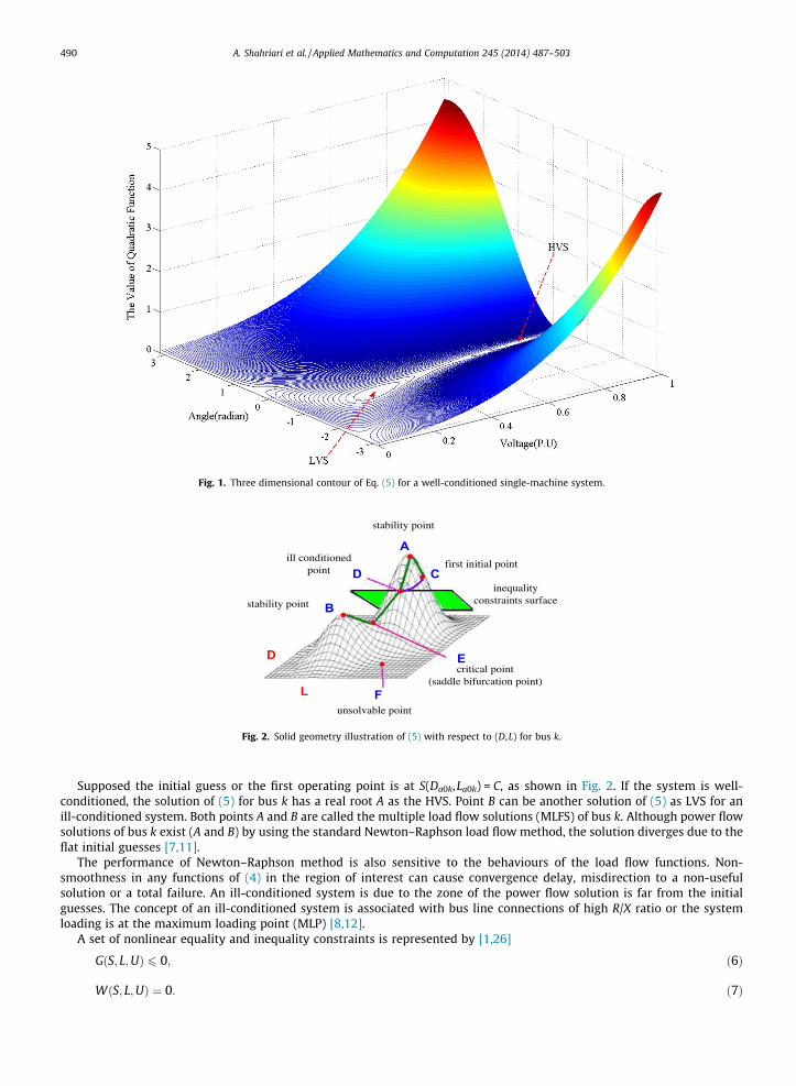
Fig. 1. Three dimensional contour of Eq. (5) for a well-conditioned single-machine system.

critical point(saddle bifurcation point)

stability point

stability point

ill conditionedpoint

first initial point

inequalityconstraints surface

unsolvable point

A

B

C

F

E

L

D

D

Fig. 2. Solid geometry illustration of (5) with respect to (D,L) for bus k.

490 A. Shahriari et al. / Applied Mathematics and Computation 245 (2014) 487–503

Supposed the initial guess or the first operating point is at S(Da0k,La0k) = C, as shown in Fig. 2. If the system is well-conditioned, the solution of (5) for bus k has a real root A as the HVS. Point B can be another solution of (5) as LVS for anill-conditioned system. Both points A and B are called the multiple load flow solutions (MLFS) of bus k. Although power flowsolutions of bus k exist (A and B) by using the standard Newton–Raphson load flow method, the solution diverges due to theflat initial guesses [7,11].

The performance of Newton–Raphson method is also sensitive to the behaviours of the load flow functions. Non-smoothness in any functions of (4) in the region of interest can cause convergence delay, misdirection to a non-usefulsolution or a total failure. An ill-conditioned system is due to the zone of the power flow solution is far from the initialguesses. The concept of an ill-conditioned system is associated with bus line connections of high R/X ratio or the systemloading is at the maximum loading point (MLP) [8,12].

A set of nonlinear equality and inequality constraints is represented by [1,26]

GðS; L;UÞ 6 0; ð6Þ

WðS; L;UÞ ¼ 0: ð7Þ

A. Shahriari et al. / Applied Mathematics and Computation 245 (2014) 487–503 491

The dependent variables is controlled by U, which consists of the generated output, Q-limit violation and newly-turned ongenerator [18]. The flat surface in Fig. 2 shows a typical system constraint. The solution in the region above the flat surface(consists of points A, C and D) are supposed to be eliminated. Operating the power system close to its security margins forheavily loaded system leads the system to become unsolvable [14]. By increasing the load demand, point A is forced to movetoward points E and F. Therefore, optimal multiple load flow method (OMLFM) is implemented to obtain the solution at pointB, or the stability point [15].

2.2. Mathematically background

The OMLFM was presented as an optimal route finder of power flow solution for an ill-conditioned system. This is exe-cuted by finding the best slope from the critical initial value to the safe margin zone of voltage stability at each iterationwithout changing the dependent variables. The task of OMLFM is to adjust the size of vector [DSi] and specify an optimalvalue towards the best stability solution for an ill-conditioned system, i.e. solution at point B in Fig. 3. The new value of inde-pendent variable, D is calculated using

Diþ1 ¼ Di þ kDDi; ð8Þ

where k is the optimal multiplier. Rewriting (3) with the multiplier gives

S Dia þ DDi

a;Dib þ DDi

b

� �� SðDi

a;DibÞ � ki DDa ;Db

S� �i

DDia;DDi

b

h i� 1

2k2

i DDia;DDi

b

h iTD2

Da ;DbS

h iiDDi

a;DDib

h i¼ 0: ð9Þ

The optimal multiplier is found by minimising the cost function of (9) with respect to the multiplier as follows,

L ¼ 12

S Dia þ DDi

a;Dib þ DDi

b

� �� SðDi

a;DibÞ þ ki DDa ;Db

S� �i

DDia;DDi

b

h iþ 1

2k2

i DDia;DDi

b

h iTD2

Da ;DbS

h iiDDi

a;DDib

h i� �2

: ð10Þ

Simplifying the term,

L ¼ 12

aþ bkþ k2c� �T

aþ bkþ k2c� �

¼ 12

aT aþ 2aT bkþ ðbT bþ 2cT aÞk2 þ 2bT ck3 þ ccTk4h i

; ð11Þ

where

a ¼ S Dia þ DDi

a;Dib þ DDi

b

� �� S Di

a;Dib

� �;

b ¼ DDa ;DbS

� �iDDi

a;DDib

h i;

c ¼ 12

k2i Di

Da;Di

Db

h iTD2

Da ;DbS

h iiDi

Da;Di

Db

h i:

For simplification according to SNRLF, b = �a [18]. The result is a scalar cubic function of k,

dLdk¼ aT bkþ bT bþ 2cT a

� �kþ 3bT ck2 þ 2ccTk3; ð12Þ

where L is the cost function and is called the energy function of power system (EFPS). Eq. (12) is called the optimisationenergy function (OEF).

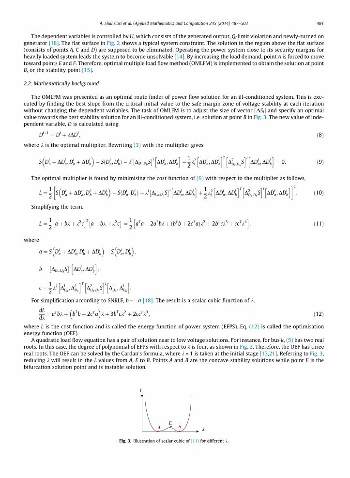
A quadratic load flow equation has a pair of solution near to low voltage solutions. For instance, for bus k, (5) has two realroots. In this case, the degree of polynomial of EFPS with respect to k is four, as shown in Fig. 2. Therefore, the OEF has threereal roots. The OEF can be solved by the Cardan’s formula, where k = 1 is taken at the initial stage [13,21]. Referring to Fig. 3,reducing k will result in the L values from A, E to B. Points A and B are the concave stability solutions while point E is thebifurcation solution point and is instable solution.

λ

Fig. 3. Illustration of scalar cubic of (11) for different k.

492 A. Shahriari et al. / Applied Mathematics and Computation 245 (2014) 487–503

Suppose that k1, k2 and k3 are corresponding to points A, E and B respectively. For example, if the OEF has two imaginaryroots and one real root, with the real root is k1. The classical algorithm of OMLFM is as follows

1. Solve SNRLF at first iteration.2. Calculate OEF.3. If OEF has a real root, go to step 4. Else, go to step 6.4. Modify the mismatch vector of independent variables in next iteration.5. If the convergence of EFPS is less than the given tolerance, the process is stopped. Else, go to step 2.6. Select the smallest root (the closest root to one is selected in vicinity of MLP) of OEF as desirable optimal multiplier and go

to step 4.

It is not guaranteed that the LVS found by the classical OMLFM is the critical solution point, as it is likely to be bifurcatedand vanished before the voltage decreases. Furthermore, due to the unavailability of any prior information about the locationof LVS, choosing a good search direction is difficult. For any load demand that is away from the MLP value, the operationpoint of the system is away from the EFPS optimum point. In a rectangular coordinate model, switching all PV type busesto PQ type buses in order to neglect extra voltage mismatch equations is problematic.

3. The proposed method

It has been shown that the mismatch vector of SNRLF is satisfied by OMLFM in low voltage solution points [13,21]. SinceaTa = 0, by satisfying the constraint of SNRLF, (12) is rewritten as

k bT bþ 2cT a� �

þ 3bT ckþ 2ccTk2� �

¼ 0: ð13Þ

The middle real root of OEF is corresponded to a singular point on a straight line connecting a pair of low voltage solu-tions. k = 0 is the multiplier of the operable power solution, which equals to the operation point. Rewriting (13),

bT bþ 2cT a� �

þ 3bT ckþ 2ccTk2� �

¼ 0;

t1 þ t2kþ t3k2� ¼ 0; ð14Þ

where

t1 ¼ bT bþ 2cT d; t2 ¼ 3bT c; t3 ¼ 2ccT :

The real roots of (14) are given by

ðk1; k2Þ ¼�t2 �

ffiffiffiffiffiffiffiffiffiffiffiffiffiffiffiffiffiffiffiffiffit2

2 � 4t1t3

q2t3

: ð15Þ

The following results are obtained:

1. The closest root to zero is considered as the local maximum of EFPS.2. The root further than zero is considered as the local minimum of EFPS.

In this work, the concavity theorems of power flow feasibility boundary have been utilised based on the fixed point testtheory [18,26]. It has been shown that the maximum number of EFPS solutions on the straight line between two operableand low voltage solutions of (9) is two. Therefore, only a real optimum solution exists for EFPS in the vicinity of MLP in astate space of load flow equations. The proof is as follows, if S(D + kDD) equals to zero, then the absolute value of (12)becomes

¼ aT aþ 2aT bkþ bT bþ 2cT a� �

k2 þ 2bT ck3 þ ccTk4h i

¼ bT bþ 2cT a� �

k2 þ 2bT ck3 þ ccTk4h i

¼ t1 þ t5kþ t6k2�

k2; ð16Þ

where t5 ¼ 2bT c and t6 ¼ ccT . a, b and c are function of DD. If and only if the direction of DD is not equal to zero, EFPS equalsto zero in two cases, where

k2 ¼ 0; ð17Þ

t1 þ t5kþ t6k2 ¼ 0: ð18Þ

The original solution, D = D0 is presented in the first case. The second case is when D – D0, which lies on the straight linewith DD. Due to EFPS in (11) and (18) are directed by k and DD, the minimum solution point of B in (18) (this is correspondedto the minimum point of EFPS with respect to k) is

A. Shahriari et al. / Applied Mathematics and Computation 245 (2014) 487–503 493

@E@k¼ 2t6kþ t5 ¼ 0! koptimal ¼ �

t5

2t6: ð19Þ

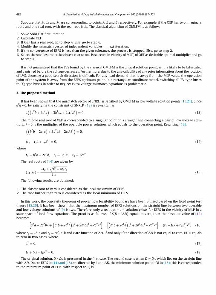
Thus, based on the fixed point theory, the trajectory path of the studied bus voltage (D) is solved in a fixed operation pointas the optimum or concave point. This is illustrated in Fig. 4. Referring to Fig. 4, point A0 is the exact optimal multiplier ofEFPS that is calculated by (19). This point may be corresponded to point A in Fig. 3 and is the indicator coefficient. However,the indicator coefficient is modified in term of higher load demands in power system case study. Thus, another optimal mul-tiplier A00 can be the indicator coefficient of the test results, which are shown in Section 4.

4. Case study

The case study involves the standard IEEE 57, 118 and 300-bus systems. To study the efficiency of the proposed method,different loading point of the systems are tested. The active and reactive load demand models in [8] are used to find the max-imum loading point of the system using

P ¼ P0 þ cP; ð20Þ

Q ¼ Q0 þ cP; ð21Þ

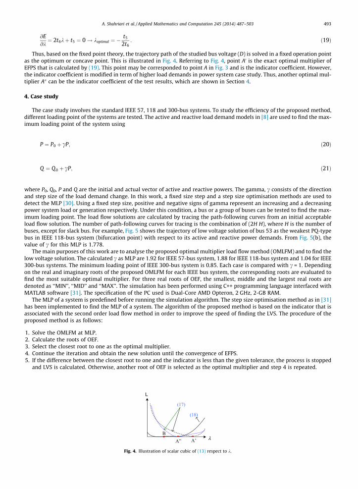
where P0, Q0, P and Q are the initial and actual vector of active and reactive powers. The gamma, c consists of the directionand step size of the load demand change. In this work, a fixed size step and a step size optimisation methods are used todetect the MLP [30]. Using a fixed step size, positive and negative signs of gamma represent an increasing and a decreasingpower system load or generation respectively. Under this condition, a bus or a group of buses can be tested to find the max-imum loading point. The load flow solutions are calculated by tracing the path-following curves from an initial acceptableload flow solution. The number of path-following curves for tracing is the combination of (2H H), where H is the number ofbuses, except for slack bus. For example, Fig. 5 shows the trajectory of low voltage solution of bus 53 as the weakest PQ-typebus in IEEE 118-bus system (bifurcation point) with respect to its active and reactive power demands. From Fig. 5(b), thevalue of c for this MLP is 1.778.

The main purposes of this work are to analyse the proposed optimal multiplier load flow method (OMLFM) and to find thelow voltage solution. The calculated c as MLP are 1.92 for IEEE 57-bus system, 1.88 for IEEE 118-bus system and 1.04 for IEEE300-bus systems. The minimum loading point of IEEE 300-bus system is 0.85. Each case is compared with c = 1. Dependingon the real and imaginary roots of the proposed OMLFM for each IEEE bus system, the corresponding roots are evaluated tofind the most suitable optimal multiplier. For three real roots of OEF, the smallest, middle and the largest real roots aredenoted as ‘‘MIN’’, ‘‘MID’’ and ‘‘MAX’’. The simulation has been performed using C++ programming language interfaced withMATLAB software [31]. The specification of the PC used is Dual-Core AMD Opteron, 2 GHz, 2-GB RAM.

The MLP of a system is predefined before running the simulation algorithm. The step size optimisation method as in [31]has been implemented to find the MLP of a system. The algorithm of the proposed method is based on the indicator that isassociated with the second order load flow method in order to improve the speed of finding the LVS. The procedure of theproposed method is as follows:

1. Solve the OMLFM at MLP.2. Calculate the roots of OEF.3. Select the closest root to one as the optimal multiplier.4. Continue the iteration and obtain the new solution until the convergence of EFPS.5. If the difference between the closest root to one and the indicator is less than the given tolerance, the process is stopped

and LVS is calculated. Otherwise, another root of OEF is selected as the optimal multiplier and step 4 is repeated.

λ

Fig. 4. Illustration of scalar cubic of (13) respect to k.

(b)

gamma

Vol

tage

of

Bus

53

(P.U

)

(a)gamma

Vol

tage

of

Bus

53

(P.U

)

0 0.5 1 1.5 2

1

0.6

0.4

0.8

A

1.78681.7866 1.787 1.7842 1.7874

A

0.498

0.4985

0.499

0.4995

Fig. 5. Bifurcation surface of bus 53 at MLP of the IEEE 118-bus system.

0 10 20 30 40 50 60-0.6

-0.4

-0.2

0

0.2

0.4

0.6

0.8

1

1.2

Bus Number

Vol

tage

(P.U

)

gamma=1gamma=1.92

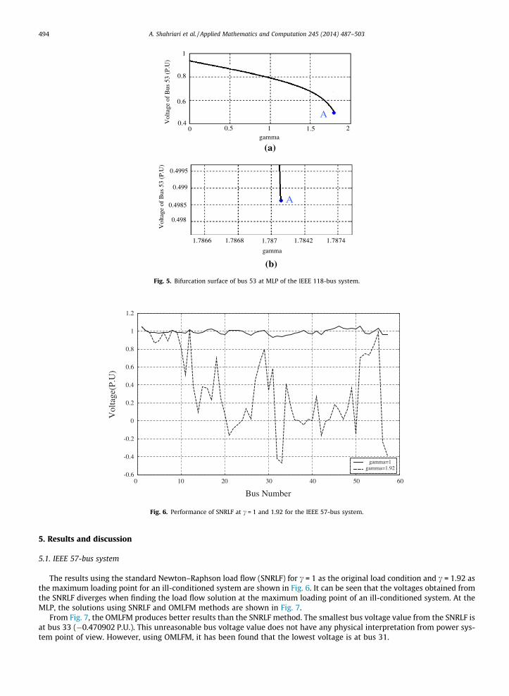
Fig. 6. Performance of SNRLF at c = 1 and 1.92 for the IEEE 57-bus system.

494 A. Shahriari et al. / Applied Mathematics and Computation 245 (2014) 487–503

5. Results and discussion

5.1. IEEE 57-bus system

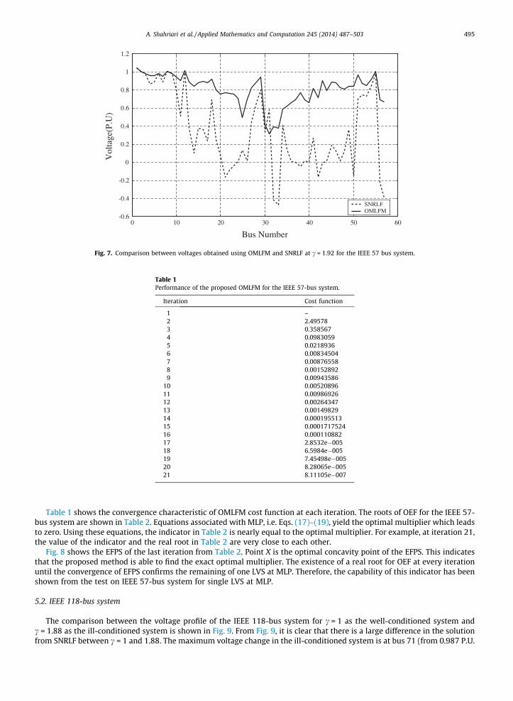
The results using the standard Newton–Raphson load flow (SNRLF) for c = 1 as the original load condition and c = 1.92 asthe maximum loading point for an ill-conditioned system are shown in Fig. 6. It can be seen that the voltages obtained fromthe SNRLF diverges when finding the load flow solution at the maximum loading point of an ill-conditioned system. At theMLP, the solutions using SNRLF and OMLFM methods are shown in Fig. 7.

From Fig. 7, the OMLFM produces better results than the SNRLF method. The smallest bus voltage value from the SNRLF isat bus 33 (�0.470902 P.U.). This unreasonable bus voltage value does not have any physical interpretation from power sys-tem point of view. However, using OMLFM, it has been found that the lowest voltage is at bus 31.

0 10 20 30 40 50 60-0.6

-0.4

-0.2

0

0.2

0.4

0.6

0.8

1

1.2

Bus Number

Vol

tage

(P.U

)

SNRLFOMLFM

Fig. 7. Comparison between voltages obtained using OMLFM and SNRLF at c = 1.92 for the IEEE 57 bus system.

Table 1Performance of the proposed OMLFM for the IEEE 57-bus system.

Iteration Cost function

1 –2 2.495783 0.3585674 0.09830595 0.02189366 0.008345047 0.008765588 0.001528929 0.00943586

10 0.0052089611 0.0098692612 0.0026434713 0.0014982914 0.00019551315 0.000171752416 0.00011088217 2.8532e�00518 6.5984e�00519 7.45498e�00520 8.28065e�00521 8.11105e�007

A. Shahriari et al. / Applied Mathematics and Computation 245 (2014) 487–503 495

Table 1 shows the convergence characteristic of OMLFM cost function at each iteration. The roots of OEF for the IEEE 57-bus system are shown in Table 2. Equations associated with MLP, i.e. Eqs. (17)–(19), yield the optimal multiplier which leadsto zero. Using these equations, the indicator in Table 2 is nearly equal to the optimal multiplier. For example, at iteration 21,the value of the indicator and the real root in Table 2 are very close to each other.

Fig. 8 shows the EFPS of the last iteration from Table 2. Point X is the optimal concavity point of the EFPS. This indicatesthat the proposed method is able to find the exact optimal multiplier. The existence of a real root for OEF at every iterationuntil the convergence of EFPS confirms the remaining of one LVS at MLP. Therefore, the capability of this indicator has beenshown from the test on IEEE 57-bus system for single LVS at MLP.

5.2. IEEE 118-bus system

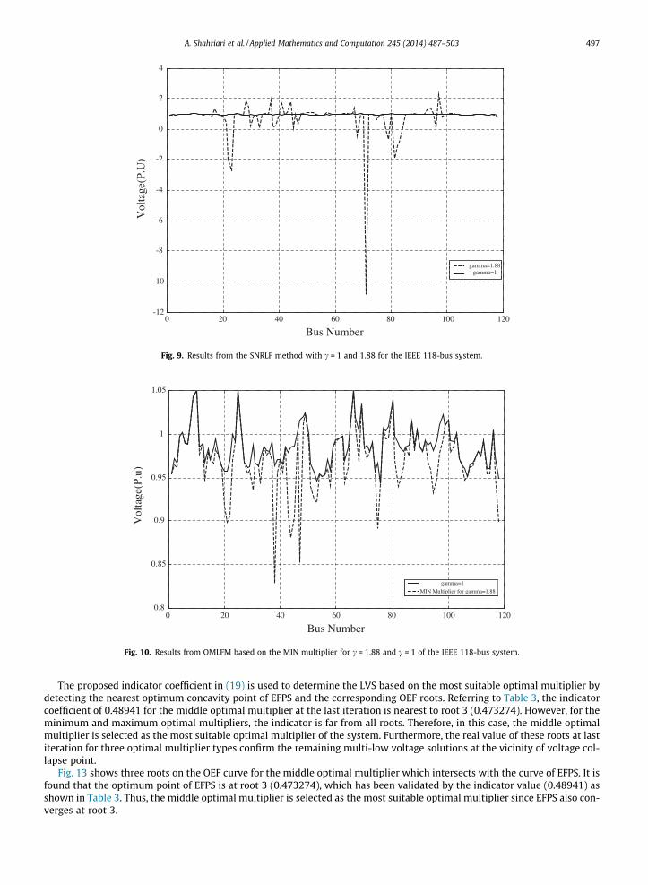
The comparison between the voltage profile of the IEEE 118-bus system for c = 1 as the well-conditioned system andc = 1.88 as the ill-conditioned system is shown in Fig. 9. From Fig. 9, it is clear that there is a large difference in the solutionfrom SNRLF between c = 1 and 1.88. The maximum voltage change in the ill-conditioned system is at bus 71 (from 0.987 P.U.

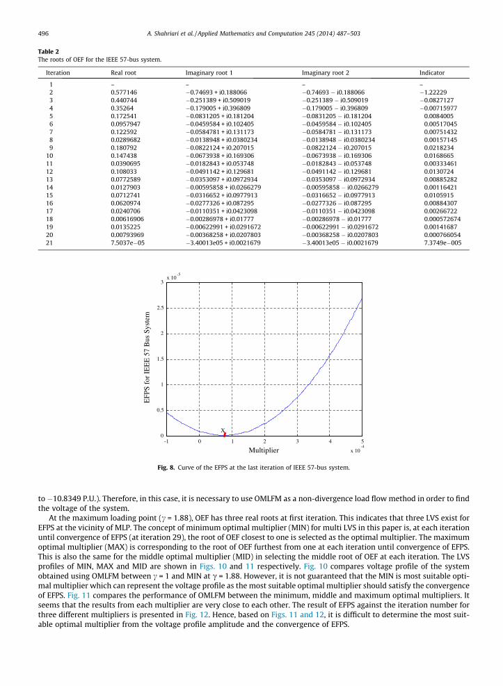
Table 2The roots of OEF for the IEEE 57-bus system.

Iteration Real root Imaginary root 1 Imaginary root 2 Indicator

1 – – – –2 0.577146 �0.74693 + i0.188066 �0.74693 � i0.188066 �1.222293 0.440744 �0.251389 + i0.509019 �0.251389 � i0.509019 �0.08271274 0.35264 �0.179005 + i0.396809 �0.179005 � i0.396809 �0.007159775 0.172541 �0.0831205 + i0.181204 �0.0831205 � i0.181204 0.00840056 0.0957947 �0.0459584 + i0.102405 �0.0459584 � i0.102405 0.005170457 0.122592 �0.0584781 + i0.131173 �0.0584781 � i0.131173 0.007514328 0.0289682 �0.0138948 + i0.0380234 �0.0138948 � i0.0380234 0.001571459 0.180792 �0.0822124 + i0.207015 �0.0822124 � i0.207015 0.0218234

10 0.147438 �0.0673938 + i0.169306 �0.0673938 � i0.169306 0.016866511 0.0390695 �0.0182843 + i0.053748 �0.0182843 � i0.053748 0.0033346112 0.108033 �0.0491142 + i0.129681 �0.0491142 � i0.129681 0.013072413 0.0772589 �0.0353097 + i0.0972934 �0.0353097 � i0.0972934 0.0088528214 0.0127903 �0.00595858 + i0.0266279 �0.00595858 � i0.0266279 0.0011642115 0.0712741 �0.0316652 + i0.0977913 �0.0316652 � i0.0977913 0.010591516 0.0620974 �0.0277326 + i0.087295 �0.0277326 � i0.087295 0.0088430717 0.0240706 �0.0110351 + i0.0423098 �0.0110351 � i0.0423098 0.0026672218 0.00616906 �0.00286978 + i0.01777 �0.00286978 � i0.01777 0.00057267419 0.0135225 �0.00622991 + i0.0291672 �0.00622991 � i0.0291672 0.0014168720 0.00793969 �0.00368258 + i0.0207803 �0.00368258 � i0.0207803 0.00076605421 7.5037e�05 �3.40013e05 + i0.0021679 �3.40013e05 � i0.0021679 7.3749e�005

-1 0 1 2 3 4 5

x 10-4

0

0.5

1

1.5

2

2.5

3x 10

-5

Multiplier

EFP

S fo

r IE

EE

57

Bus

Sys

tem

X

Fig. 8. Curve of the EFPS at the last iteration of IEEE 57-bus system.

496 A. Shahriari et al. / Applied Mathematics and Computation 245 (2014) 487–503

to �10.8349 P.U.). Therefore, in this case, it is necessary to use OMLFM as a non-divergence load flow method in order to findthe voltage of the system.

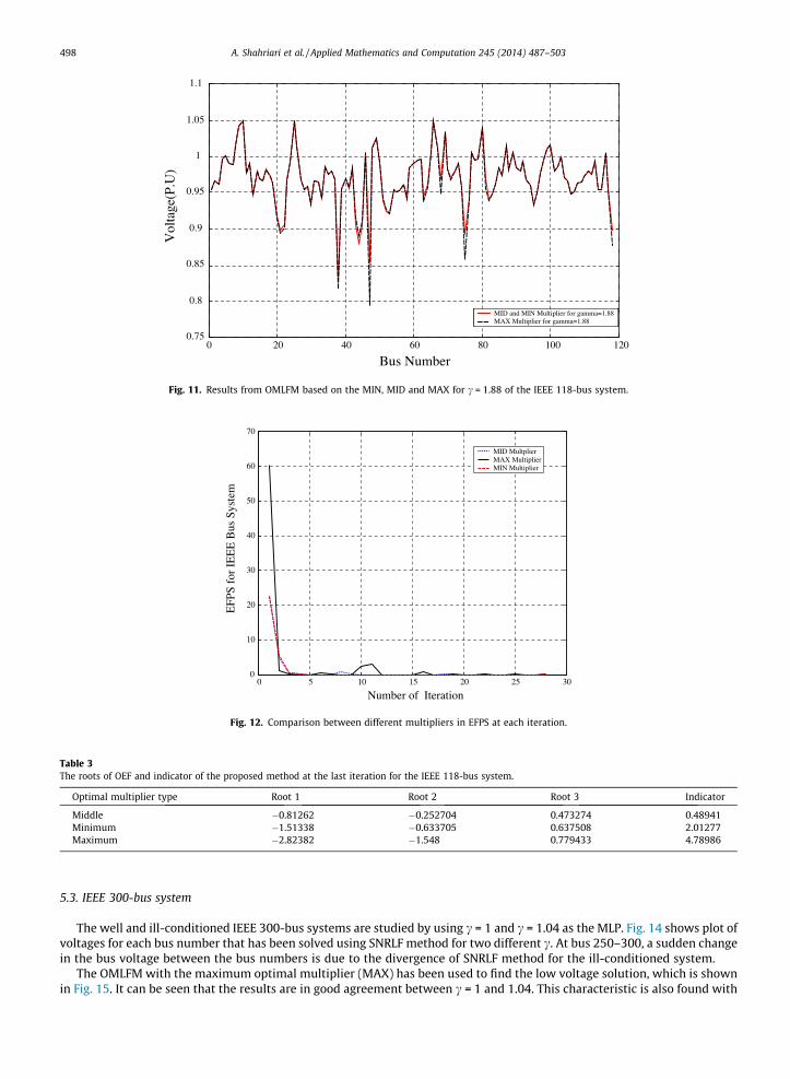
At the maximum loading point (c = 1.88), OEF has three real roots at first iteration. This indicates that three LVS exist forEFPS at the vicinity of MLP. The concept of minimum optimal multiplier (MIN) for multi LVS in this paper is, at each iterationuntil convergence of EFPS (at iteration 29), the root of OEF closest to one is selected as the optimal multiplier. The maximumoptimal multiplier (MAX) is corresponding to the root of OEF furthest from one at each iteration until convergence of EFPS.This is also the same for the middle optimal multiplier (MID) in selecting the middle root of OEF at each iteration. The LVSprofiles of MIN, MAX and MID are shown in Figs. 10 and 11 respectively. Fig. 10 compares voltage profile of the systemobtained using OMLFM between c = 1 and MIN at c = 1.88. However, it is not guaranteed that the MIN is most suitable opti-mal multiplier which can represent the voltage profile as the most suitable optimal multiplier should satisfy the convergenceof EFPS. Fig. 11 compares the performance of OMLFM between the minimum, middle and maximum optimal multipliers. Itseems that the results from each multiplier are very close to each other. The result of EFPS against the iteration number forthree different multipliers is presented in Fig. 12. Hence, based on Figs. 11 and 12, it is difficult to determine the most suit-able optimal multiplier from the voltage profile amplitude and the convergence of EFPS.

0 20 40 60 80 100 120-12

-10

-8

-6

-4

-2

0

2

4

Vol

tage

(P.U

)

Bus Number

gamma=1.88gamma=1

Fig. 9. Results from the SNRLF method with c = 1 and 1.88 for the IEEE 118-bus system.

0 20 40 60 80 100 1200.8

0.85

0.9

0.95

1

1.05

Vol

tage

(P.u

)

Bus Number

gamma=1

MIN Multiplier for gamma=1.88

Fig. 10. Results from OMLFM based on the MIN multiplier for c = 1.88 and c = 1 of the IEEE 118-bus system.

A. Shahriari et al. / Applied Mathematics and Computation 245 (2014) 487–503 497

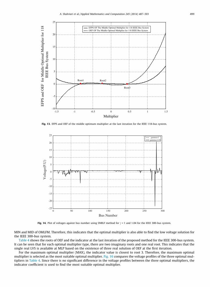
The proposed indicator coefficient in (19) is used to determine the LVS based on the most suitable optimal multiplier bydetecting the nearest optimum concavity point of EFPS and the corresponding OEF roots. Referring to Table 3, the indicatorcoefficient of 0.48941 for the middle optimal multiplier at the last iteration is nearest to root 3 (0.473274). However, for theminimum and maximum optimal multipliers, the indicator is far from all roots. Therefore, in this case, the middle optimalmultiplier is selected as the most suitable optimal multiplier of the system. Furthermore, the real value of these roots at lastiteration for three optimal multiplier types confirm the remaining multi-low voltage solutions at the vicinity of voltage col-lapse point.

Fig. 13 shows three roots on the OEF curve for the middle optimal multiplier which intersects with the curve of EFPS. It isfound that the optimum point of EFPS is at root 3 (0.473274), which has been validated by the indicator value (0.48941) asshown in Table 3. Thus, the middle optimal multiplier is selected as the most suitable optimal multiplier since EFPS also con-verges at root 3.

0 20 40 60 80 100 1200.75

0.8

0.85

0.9

0.95

1

1.05

1.1

Vol

tage

(P.U

)

MID and MIN Multiplier for gamma=1.88MAX Multiplier for gamma=1.88

Bus Number

Fig. 11. Results from OMLFM based on the MIN, MID and MAX for c = 1.88 of the IEEE 118-bus system.

0 5 10 15 20 25 300

10

20

30

40

50

60

70

Number of Iteration

EFP

S fo

r IE

EE

Bus

Sys

tem

MID Multplier MAX MultiplierMIN Multiplier

Fig. 12. Comparison between different multipliers in EFPS at each iteration.

Table 3The roots of OEF and indicator of the proposed method at the last iteration for the IEEE 118-bus system.

Optimal multiplier type Root 1 Root 2 Root 3 Indicator

Middle �0.81262 �0.252704 0.473274 0.48941Minimum �1.51338 �0.633705 0.637508 2.01277Maximum �2.82382 �1.548 0.779433 4.78986

498 A. Shahriari et al. / Applied Mathematics and Computation 245 (2014) 487–503

5.3. IEEE 300-bus system

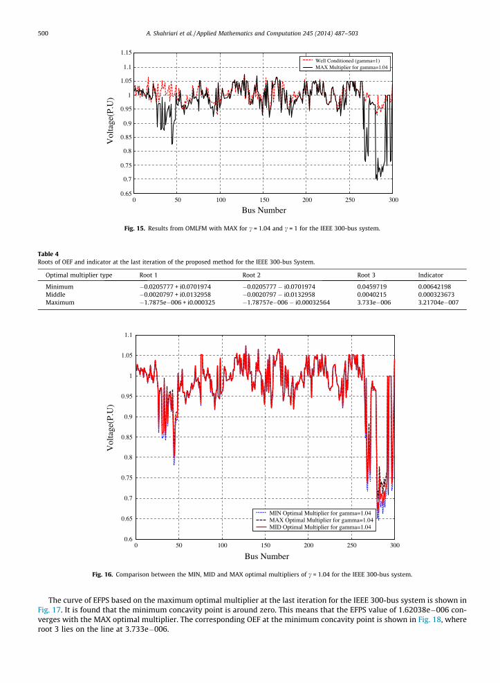
The well and ill-conditioned IEEE 300-bus systems are studied by using c = 1 and c = 1.04 as the MLP. Fig. 14 shows plot ofvoltages for each bus number that has been solved using SNRLF method for two different c. At bus 250–300, a sudden changein the bus voltage between the bus numbers is due to the divergence of SNRLF method for the ill-conditioned system.

The OMLFM with the maximum optimal multiplier (MAX) has been used to find the low voltage solution, which is shownin Fig. 15. It can be seen that the results are in good agreement between c = 1 and 1.04. This characteristic is also found with

-1.5 -1 -0.5 0 0.5 1 1.5-10

-5

0

5

10

15

20

25

Multiplier

EFP

S an

d O

EF

for

Mid

dle

Opt

imal

Mul

tiplie

r fo

r 11

8

I

EE

E B

us S

yste

m

EFPS OF The Middle Optimal Multiplier for 118 IEEE Bus SystemOEF OF The Middle Optimal Multiplier for 118 IEEE Bus System

Root1 Root2

Root3

Fig. 13. EFPS and OEF of the middle optimum multiplier at the last iteration for the IEEE 118-bus system.

0 50 100 150 200 250 300-25

-20

-15

-10

-5

0

5

10

15

20

25

Bus Number

Vol

tage

(P.U

)

gamma=1.04gamma=1

Fig. 14. Plot of voltages against bus number using SNRLF method for c = 1 and 1.04 for the IEEE 300-bus system.

A. Shahriari et al. / Applied Mathematics and Computation 245 (2014) 487–503 499

MIN and MID of OMLFM. Therefore, this indicates that the optimal multiplier is also able to find the low voltage solution forthe IEEE 300-bus system.

Table 4 shows the roots of OEF and the indicator at the last iteration of the proposed method for the IEEE 300-bus system.It can be seen that for each optimal multiplier type, there are two imaginary roots and one real root. This indicates that thesingle real LVS is available at MLP based on the existence of three real solution of OEF at the first iteration.

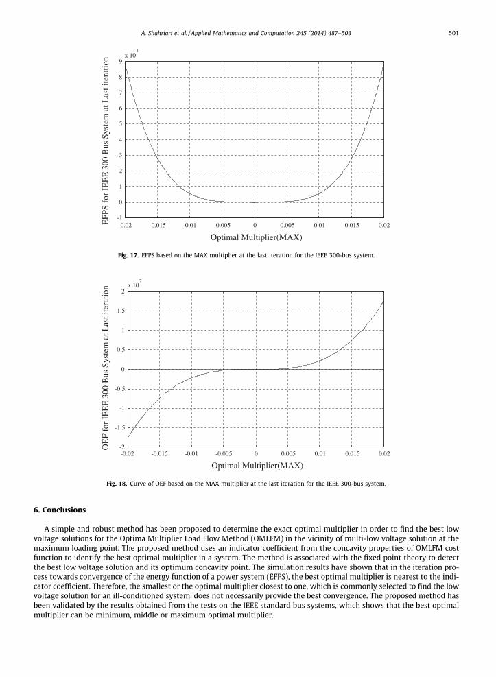
For the maximum optimal multiplier (MAX), the indicator value is closest to root 3. Therefore, the maximum optimalmultiplier is selected as the most suitable optimal multiplier. Fig. 16 compares the voltage profiles of the three optimal mul-tipliers in Table 4. Since there is no significant difference in the voltage profiles between the three optimal multipliers, theindicator coefficient is used to find the most suitable optimal multiplier.

0 50 100 150 200 250 3000.65

0.7

0.75

0.8

0.85

0.9

0.95

1

1.05

1.1

1.15

Bus Number

Vol

tage

(P.U

)

Well Conditioned (gamma=1) MAX Multiplier for gamma=1.04

Fig. 15. Results from OMLFM with MAX for c = 1.04 and c = 1 for the IEEE 300-bus system.

Table 4Roots of OEF and indicator at the last iteration of the proposed method for the IEEE 300-bus System.

Optimal multiplier type Root 1 Root 2 Root 3 Indicator

Minimum �0.0205777 + i0.0701974 �0.0205777 � i0.0701974 0.0459719 0.00642198Middle �0.0020797 + i0.0132958 �0.0020797 � i0.0132958 0.0040215 0.000323673Maximum �1.7875e�006 + i0.000325 �1.78757e�006 � i0.00032564 3.733e�006 3.21704e�007

0 50 100 150 200 250 3000.6

0.65

0.7

0.75

0.8

0.85

0.9

0.95

1

1.05

1.1

Vol

tage

(P.U

)

MIN Optimal Multiplier for gamma=1.04MAX Optimal Multiplier for gamma=1.04MID Optimal Multiplier for gamma=1.04

Bus Number

Fig. 16. Comparison between the MIN, MID and MAX optimal multipliers of c = 1.04 for the IEEE 300-bus system.

500 A. Shahriari et al. / Applied Mathematics and Computation 245 (2014) 487–503

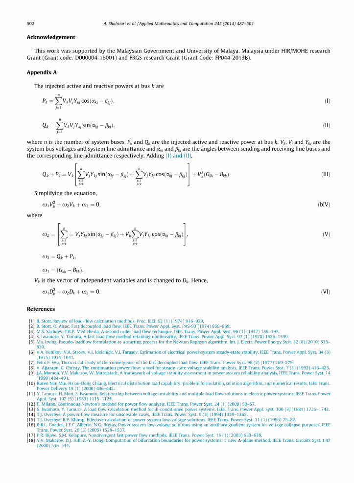
The curve of EFPS based on the maximum optimal multiplier at the last iteration for the IEEE 300-bus system is shown inFig. 17. It is found that the minimum concavity point is around zero. This means that the EFPS value of 1.62038e�006 con-verges with the MAX optimal multiplier. The corresponding OEF at the minimum concavity point is shown in Fig. 18, whereroot 3 lies on the line at 3.733e�006.

-0.02 -0.015 -0.01 -0.005 0 0.005 0.01 0.015 0.02-1

0

1

2

3

4

5

6

7

8

9x 10

4

EFP

S fo

r IE

EE

300

Bus

Sys

tem

at L

ast i

tera

tion

Optimal Multiplier(MAX)

Fig. 17. EFPS based on the MAX multiplier at the last iteration for the IEEE 300-bus system.

-0.02 -0.015 -0.01 -0.005 0 0.005 0.01 0.015 0.02-2

-1.5

-1

-0.5

0

0.5

1

1.5

2x 10

7

OE

F fo

r IE

EE

300

Bus

Sys

tem

at L

ast i

tera

tion

Optimal Multiplier(MAX)

Fig. 18. Curve of OEF based on the MAX multiplier at the last iteration for the IEEE 300-bus system.

A. Shahriari et al. / Applied Mathematics and Computation 245 (2014) 487–503 501

6. Conclusions

A simple and robust method has been proposed to determine the exact optimal multiplier in order to find the best lowvoltage solutions for the Optima Multiplier Load Flow Method (OMLFM) in the vicinity of multi-low voltage solution at themaximum loading point. The proposed method uses an indicator coefficient from the concavity properties of OMLFM costfunction to identify the best optimal multiplier in a system. The method is associated with the fixed point theory to detectthe best low voltage solution and its optimum concavity point. The simulation results have shown that in the iteration pro-cess towards convergence of the energy function of a power system (EFPS), the best optimal multiplier is nearest to the indi-cator coefficient. Therefore, the smallest or the optimal multiplier closest to one, which is commonly selected to find the lowvoltage solution for an ill-conditioned system, does not necessarily provide the best convergence. The proposed method hasbeen validated by the results obtained from the tests on the IEEE standard bus systems, which shows that the best optimalmultiplier can be minimum, middle or maximum optimal multiplier.

502 A. Shahriari et al. / Applied Mathematics and Computation 245 (2014) 487–503

Acknowledgement

This work was supported by the Malaysian Government and University of Malaya, Malaysia under HIR/MOHE researchGrant (Grant code: D000004-16001) and FRGS research Grant (Grant Code: FP044-2013B).

Appendix A

The injected active and reactive powers at bus k are

Pk ¼Xn

j¼1

VkVjYkj cosðakj � bkjÞ; ðIÞ

Qk ¼Xn

j¼1

VkVjYkj sinðakj � bkjÞ; ðIIÞ

where n is the number of system buses, Pk and Qk are the injected active and reactive power at bus k, Vk, Vj and Ykj are thesystem bus voltages and system line admittance and aki and bkj are the angles between sending and receiving line buses andthe corresponding line admittance respectively. Adding (I) and (II),

Qk þ Pk ¼ Vk

Xn

j¼1j–k

VjYkj sinðakj � bkjÞ þXn

j¼1j–k

V jYkj cosðakj � bkjÞ

264

375þ V2

kðGkk � BkkÞ: ðIIIÞ

Simplifying the equation,

x1V2k þx2Vk þx3 ¼ 0; ðbIVÞ

where

x2 ¼Xn

j¼1j–k

¼ VjYkj sinðakj � bkjÞ þ Vk

Xn

j¼1j–k

V jYkj cosðakj � bkjÞ

264

375; ðVÞ

x3 ¼ Q k þ Pk;

x1 ¼ ðGkk � BkkÞ:

Vk is the vector of independent variables and is changed to Dk. Hence,

x1D2k þx2Dk þx3 ¼ 0: ðVIÞ

References

[1] B. Stott, Review of load-flow calculation methods, Proc. IEEE 62 (1) (1974) 916–929.[2] B. Stott, O. Alsac, Fast decoupled load flow, IEEE Trans. Power Appl. Syst. PAS-93 (1974) 859–869.[3] M.S. Sachdev, T.K.P. Medicherla, A second order load flow technique, IEEE Trans. Power Appl. Syst. 96 (1) (1977) 189–197.[4] S. Iwamoto, Y. Tamura, A fast load flow method retaining nonlinearity, IEEE Trans. Power Appl. Syst. 97 (1) (1978) 1586–1599.[5] Ma. Irving, Pseudo-loadflow formulation as a starting process for the Newton Raphson algorithm, Int. J. Electr. Power Energy Syst. 32 (8) (2010) 835–

839.[6] V.A. Venikov, V.A. Stroev, V.I. Idelchick, V.I. Tarasov, Estimation of electrical power-system steady-state stability, IEEE Trans. Power Appl. Syst. 94 (3)

(1975) 1034–1041.[7] Felix F. Wu, Theoretical study of the convergence of the fast decoupled load flow, IEEE Trans. Power Syst. 96 (2) (1977) 269–275.[8] V. Ajjarapu, C. Christy, The continuation power flow: a tool for steady state voltage stability analysis, IEEE Trans. Power Syst. 7 (1) (1992) 416–423.[9] J.A. Momoh, Y.V. Makarov, W. Mittelstadt, A framework of voltage stability assessment in power system reliability analysis, IEEE Trans. Power Syst. 14

(1999) 484–491.[10] Karen Nan Miu, Hsiao-Dong Chiang, Electrical distribution load capability: problem formulation, solution algorithm, and numerical results, IEEE Trans.

Power Delivery 15 (1) (2000) 436–442.[11] Y. Tamura, H. Mori, S. Iwamoto, Relationship between voltage instability and multiple load flow solutions in electric power systems, IEEE Trans. Power

Appl. Syst. 102 (5) (1983) 1115–1125.[12] F. Milano, Continuous Newton’s method for power flow analysis, IEEE Trans. Power Syst. 24 (1) (2009) 50–57.[13] S. Iwamoto, Y. Tamura, A load flow calculation method for ill-conditioned power systems, IEEE Trans. Power Appl. Syst. 100 (3) (1981) 1736–1743.[14] T.J. Overbye, A power flow measure for unsolvable cases, IEEE Trans. Power Syst. 9 (3) (1994) 1359–1365.[15] T.J. Overbye, R.P. Klump, Effective calculation of power system low-voltage solutions, IEEE Trans. Power Syst. 11 (1) (1996) 75–82.[16] R.B.L. Guedes, L.F.C. Alberto, N.G. Bretas, Power system low-voltage solutions using an auxiliary gradient system for voltage collapse purposes, IEEE

Trans. Power Syst. 20 (3) (2005) 1528–1537.[17] P.R. Bijwe, S.M. Kelapure, Nondivergent fast power flow methods, IEEE Trans. Power Syst. 18 (1) (2003) 633–638.[18] Y.V. Makarov, D.J. Hill, Z.-Y. Dong, Computation of bifurcation boundaries for power systems: a new D-plane method, IEEE Trans. Circuits Syst. I 47

(2000) 536–544.

A. Shahriari et al. / Applied Mathematics and Computation 245 (2014) 487–503 503

[19] R.J. Avalos, C.A. Cañizares, F. Milano, A. Conejo, Equivalency of continuation and optimization methods to determine saddle-node and limit inducedbifurcations in power systems, IEEE Trans. Power Circuits Syst. 56 (1) (2009) 210–223.

[20] S. Ayasun, C.O. Nwankpa, H.G. Kwatny, Computation of singular and singularity induced bifurcation points of differential-algebraic power systemmodel, IEEE Trans. Circuits Syst. 51 (2004) 1525–1538.

[21] K. Iba, H. Suzuki, M. Egawa, T. Watanabe, A method for finding a pair of multiple load flow solutions in bulk power systems, IEEE Trans. Power Syst. 5(2) (1990) 582–591.

[22] L.M.C. Braz, C.A. Castro, C.A.F. Murari, A critical evaluation of step size optimization based load flow methods, IEEE Trans. Power Syst. 15 (1) (2000)202–207.

[23] Y.V. Marakov, Z.Y. Dong, D.J. Hill, On concavity of power flow feasibility boundary, IEEE Trans. Power Syst. 23 (2) (2008).[24] J.E. Tate, T.J. Overbye, A comparison of the optimal multiplier in polar and rectangular coordinates, IEEE Trans. Power Syst. 20 (4) (2005) 1667–1674.[25] L.M.C. Braz, C.A. Castro, C.A.F. Murari, A critical evaluation of step size optimization based load flow methods, IEEE Trans. Power Syst. vol. 15 (1)

(February 2000) 202–207.[26] Y.V. Makarov, D.J. Hill, I.A. Hiskens, Properties of quadratic equations and their application to power system analysis, Int. J. Electr. Power Energy Syst.

22 (2000) 313–323.[27] Y.V. Makarov, I.A. Hiskens, D.J. Hill, Study of multisolution quadratic load flow problems and applied Newton-Raphson like methods, in: Proceedings of

the IEEE International Symposium on Circuits and Systems, Seattle, Washington, April/May 1995, paper No. 541.[28] M.D. Schaffer, D.J. Tylavsky, A nondiverging polar form Newton-based power flow, IEEE Trans. Ind. Appl. 24 (1) (1988) 870–877.[29] R.A. Jabr, A conic quadratic format for the load flow equations of meshed networks, IEEE Trans. Power Syst. 22 (4) (2007) 2285–2286.[30] C.H. Fujisawa, C.A. Castro, Simple method for computing power system maximum loading conditions, in: IEEE Bucharest Conference, 2009.[31] K.M. Nor, H. Mokhlis, T.A. Gani, Reusability techniques in load flow analysis computer program, IEEE Trans. Power Syst. 19 (4) (2004) 1754–1762.