Optimal management of replacement heifers in a beef herd: A model for simultaneous optimization of rearing and breeding decisions

A. H. Stygar, A. R. Kristensen and J. Makulskaoptimization of rearing and breeding decisions

Optimal management of replacement heifers in a beef herd: A model for simultaneous

doi: 10.2527/jas.2010-75352014, 92:3636-3649.J ANIM SCI

http://www.journalofanimalscience.org/content/92/8/3636the World Wide Web at:

The online version of this article, along with updated information and services, is located on

www.asas.org

by guest on September 11, 2014www.journalofanimalscience.orgDownloaded from by guest on September 11, 2014www.journalofanimalscience.orgDownloaded from

http://http://www.journalofanimalscience.org/content/92/8/3636

http://www.asas.org/

http://www.journalofanimalscience.org/


3636

Optimal management of replacement heifers in a beef herd: A model for simultaneous optimization of rearing and breeding decisions1

A. H. Stygar,*†2 A. R. Kristensen,‡ and J. Makulska†

*Economic Research, Agrifood Research Finland, Latokartanonkaari 9, 00790 Helsinki, Finland; †Department of Cattle Breeding, University of Agriculture in Krakow, 30-059 Kraków, Al. Mickiewicza 24/28, Poland; and ‡Department of Large Animal Sciences, University of Copenhagen, Grønnegårdsvej 2, DK-1870 Frederiksberg C, Denmark

ABSTRACT: The aim of this study was to provide farmers an efficient tool for supporting optimal deci-sions in the beef heifer rearing process. The complexity of beef heifer management prompted the development of a model including decisions on the feeding level dur-ing prepuberty (age <10 mo), the time of weaning (age, BW, calendar month), the feeding level during the repro-ductive period (age ≥10 mo), and time of breeding (age, BW, and calendar month). The model was formulated as 3-level hierarchic Markov process. A founder level of the model has 12 states resembling all possible birth months of a heifer. Based on the birth month information from the founder level, for the indoor season (November to April) and outdoor season (May to October), feeding and breeding costs (natural service cost in the outdoor and AI cost in the indoor season) were applied. The optimal rearing strategy was found by maximizing the total discounted net revenues from the predicted future productivity of the Polish Limousine heifers defined as the cumulative BW of calves born from a cow calved until the age of 5 yr, standardized on the 210th day of age. According to the modeled optimal policy, heif-ers fed during the whole rearing period at the ADG of

810 g/d and generally weaned after the maximum suck-ling period of 9 mo should already be bred at the age of 13.2 mo and BW constituting 55.6% of the average mature BW. Based on the optimal strategy, 52% of all heifers conceived from May to July and calved from February to April. This optimal rearing pattern result-ed in an average net return of EUR 311.6 per pregnant heifer. It was found that the economic efficiency of beef operations can be improved by applying different herd management practices to those currently used in Poland. Breeding at 55.6% of the average mature BW, after a shorter and less expensive rearing period, resulted in an increase in the average net return per heifer by almost 18% compared to the conventional system, in which heifers were bred after attaining 65% of the mature BW. Extension of the rearing period by 2.5 mo (breeding at the age 15.7 mo), due to a prepubertal growth rate lowered by 200 g, reduced the average net return per heifer by 6.2% compared to the results obtained under the basic model assumptions. In the future, the model may also be extended to investigate additional aspects of the beef heifer development, such as the environmental impacts of various heifer management decisions.

Key words: beef heifers, Markov decision process, optimization

© 2014 American Society of Animal Science. All rights reserved. J. Anim. Sci. 2014.92:3636–3649 doi:10.2527/jas2010-7535

INTRODUCTION

To optimize the heifer-rearing process, a beef herd manager, given the available information and all of the biological, technical, economic, or personal constraints, must decide on the feeding level during prepuberty and in the reproductive period as well as the time of wean-ing and breeding (age, BW, and calendar month).

Herd managers often apply general norms, stan-dards, and recommendations (reviewed by Patterson et al., 1992). For example, for many years, a rule of thumb

1This study was supported by the Polish Ministry of Science and Higher Education (project no. N N311 537340). The authors acknowledge the Polish Association of Beef Cattle Breeders and Producers for providing data and valuable information regarding beef production. Moreover, we would like to thank beef farms surveyed during field studies, namely the Cooperative “Agrofirm” Witkowo, Agro Provimi Sp. z o.o. in Bieganów, and Radan Weu Sp. z o.o. in Tuchola Żarska for granting us access to production data and valuable communication regarding the practical problems of beef heifer management. The authors thank Professor Henryk Grodzki from Warsaw University of Life Sciences and Janne Helin from Economic Research, MTT Agrifood Research Finland, for valuable comments.

2Corresponding author: [email protected] December 20, 2013.Accepted June 2, 2014.

by guest on September 11, 2014www.journalofanimalscience.orgDownloaded from


Beef heifer model 3637

was the feeding of replacement heifers to achieve 60 to 65% of their expected mature BW by the start of the first breeding period (Patterson et al., 1992) to ensure satis-factory pregnancy rates. However, analyses performed by Funston and Deutscher (2004) and Roberts et al. (2009), among others, indicate that the increased feeding costs of conventionally raised heifers are not compensated by a noticeable improvement in their subsequent reproduction and calf performance compared to those bred at a lower BW, ranging from 50 to 57% of the expected mature BW.

Considering the complexity of the beef heifer rearing problem, the application of mathematical modeling and programming is a more precise method for decision sup-port. Such an approach allows individual conditions to be taken into account, combining the information from dif-ferent sources and directly representing uncertainty.

Mourits et al. (1999, 2000b) successfully used the Markov decision process to support optimal decisions on the rearing and breeding of dairy heifers. These model-based studies performed on the Dutch dairy heifer popu-lation evaluated management strategies and revealed that too low a growth rate in rearing and an excessive delay in the first breeding can reduce the farmer income by about 4.5% (Mourits, 2000a). However, none of the known Markov decision process models have focused on the optimization of replacement beef heifer rearing (Stygar and Makulska, 2010).

The objective of this study was to develop a mul-tilevel hierarchic Markov model to determine the eco-nomically optimal management strategy for replace-ment beef heifers.

MATERIALS AND METHODS

Structure of the Replacement Beef Heifer Model: Stages, State Variables, and Decisions

The beef heifer model is structured as a multilevel hierarchic Markov process (MLHMP). The MLHMP is a combination of dynamic programming and Markov processes. The optimization technique used in MLHMP is a combination of value iteration in the child process and policy iteration in the founder process (Kristensen and Jørgensen, 2000).

The MLHMP procedure determines the optimal pol-icy of beef heifer rearing by maximizing the predefined objective function π(s), which represents the expected net returns per unit of output (per pregnant heifer), as follows:

1 1( ) / /s s u s s u s sr m i i i i i is p r p mp p p S S= == = ,

in which srp = average reward over stages under policy s,

smp = average physical output over stages under policy s, sip = limiting state probability under policy s, s

ir = expect-ed average reward in state i under policy s, and s

im = phys-ical output (per pregnant heifer) in state i under policy s.

The characteristics of the processes at respective lev-els of the model are summarized in Table 1. The founder process, described as level 0 of the model, has an infinite time horizon with an infinite numbers of stages. The stage length of the founder process is equal to the duration of beef heifer rearing period from birth to successful concep-tion, which is 32 mo at maximum. The state space at level 0 is defined by only 1 state variable (month of birth), which varies between animals but is constant over the entire life of a heifer. This state variable consists of 12 classes, corre-sponding to the calendar month. The heifer calendar month of birth determines the calendar month during a certain stage in a subprocess at the child level. Based on the birth month information from the founder level, for the indoor season (November to April) and outdoor season (May to October), feeding and breeding costs (natural service [NS] in the outdoor and AI in the indoor season) are applied. The only decision to be made in the founder process concerns feeding intensity, which is defined by the ADG. Under the basic model assumptions, 2 levels of daily gain in heifers were defined: 800 g/d without supplementary feeding and 1,000 g/d with supplementary feeding. This decision influ-ences the growth rate of heifers from birth to 10 mo of age.

Child level 1 represents the preweaning (suckling) period of heifer life, which is assumed to last for a maxi-mum of 9 mo. This level consists of 10 stages reflect-ing 9 mo (30.5 d/mo) of possible suckling. The length of the last suckling stage is equal to 0. Similarly to the founder level, the state space is characterized by only 1 state variable, which in this case is BW.

Body weight classes with a width of 10 kg are de-fined on the basis of the BW at birth and the feeding decision made at the founder level. The number of BW

Table 1. Characteristics of the beef heifer model structured as a multilevel hierarchic Markov processLevel Time horizon Stage State variable Level-specific decision0 Infinite Heifer rearing period Birth month Feeding level in preweaning period and in weaned stage1 Preweaning

period110 stages representing preweaning period, 1 through 9 with duration 30.5 d and 10th with duration 0

BW Weaning and feeding level in 32 stages representing reproductive cycles

2 Reproductive period

Weaned stage1 BW Continue feeding from level 032 stages representing reproductive cycles BW × reproduction status Breeding

1The preweaning period and weaned stage constitute the heifer prepuberty period.



Stygar et al.3638

classes varies from only 1 in the first stage (birth BW) to 5 in the last stage, assuming the ADG of 800 g/d, and 7, assuming the maximum ADG of 1,000 g/d. The nutrient requirements for the heifers are determined on the basis of the mean BW in the class intervals.

At the beginning of each stage (month), the decision between weaning and continuing suckling has to be made. For each state (BW) of child level 1, 4 alternatives are possible: either to wean and ensure 400, 600, or 800 g of ADG during the reproductive period (child level 2) or keep the heifer at that stage (skip the decision on weaning until the next stage). The weaning decision is also pos-sible in the first stage of the heifer life, after an adequate intake of colostrum is ensured. The weaning strategy is defined by the heifer age, BW, and month of weaning.

Child level 2, called the reproductive period, is a more detailed representation of the period lasting from heifer weaning to successful breeding. The duration of the first stage (“weaned”) varies depending on the tim-ing of the weaning decision and can last from only 1 mo up to 10 mo. Because no observations are made in this stage, only 1 state (BW class) and 1 decision (continue feeding) are defined. The weaned stage together with the preweaning period constitute the prepuberty period, cor-responding to the first 10 mo of heifer life.

After the weaned stage, the 32 reproduction stages are distinguished. They correspond to 32 reproductive cycles, each with a duration of 21 d. The states of the reproduc-tive period are defined as the combination of BW classes and reproduction status (estrus, nonestrus, pregnant, or diseased). It was assumed that the reproduction status cor-responds to the actual physical state of the animal. For ex-ample, the state “estrus” in the model represents a heifer that has reached sexual precocity and is in estrus. Similarly, the state “pregnant,” already possible in the model on the 21st day after the breeding decision, describes a heifer that would actually be diagnosed as pregnant.

Depending on the state of the heifer, different deci-sions are considered. In the state “estrus,” 2 alternative decisions, “breed” or “keep,” were defined, whereas in the state “nonestrus,” the decisions were “keep” or “re-place.” When the heifer enters the state “pregnant” or “diseased,” the decisions “wait for calving” and “replace” are made, respectively. These decisions allow the child process to skip the remaining stages and jump directly to the next stage of the founder process.

Transition Probabilities

The heifer-rearing period is represented by a sequence of stages and states. Following the Markov chain method-ology (Norris, 1998), a heifer moves from one state to the next one according to the transition probability, which only depends on the current state and the decision made.

The transition probabilities of child level 1 are cal-culated by multiplying the involuntary disposal prob-ability by the probability of attaining the assumed BW gain (assumed probabilities are presented in Table 2).

The uncertainty in child level 2 is represented by the probability of onset of puberty and the probability of conception (Table 2). At each stage, similarly to child level 1, the involuntary disposal probability and the probability of attaining the BW gain are considered.

Natural service during the outdoor season and AI dur-ing the indoor season were used. The conception prob-abilities included the estrus detection rate, conception rate after NS or AI, and early embryo losses. Due to the lack of reliable, empirical data on the influence of feeding in-tensity in rearing and BW at breeding on Limousin heifer conception probability, the values used in the model were calculated based on information from the literature. The conception probability for the heifers bred by AI, esti-mated according to Roberts et al. (2009), are presented in Table 2. The conception probability in NS were calculated by using the approach of Meaker (1984).

Costs

Since heifer rearing was treated as a separate ac-tivity in a beef herd, only the costs that can be directly assigned to this process were taken into account in the presented model. The direct costs were further split into heifer feed and nonfeed variable costs. Separation of feed costs from other costs was justified by the fact that feed costs represent the largest expense in beef produc-tion, amounting to 70 to 80% of the total direct costs (Allan, 2005). The remaining direct expenses consid-ered in the model, namely the cost of a heifer calf and heifer breeding costs, were grouped in the nonfeed vari-able costs of heifer rearing.

In the presented study, the nutrient requirements of heifers were determined according to INRA feeding standards (INRA, 1989), recommended in Poland for the formulation of the rations for ruminants.

The diet of calves reared with mothers mainly com-prises the mother’s milk and additional forage fed ad li-bitum. Therefore, to simplify, the basic feed costs of a suckling heifer calf were calculated from the costs of the rations for the suckler cow, estimated by means of the program INRAtion 4.06 (INRAtion-PrevAlim, 2008), using forage characteristics and prices from Table 3. It was assumed that rearing the calf with the mother, with-out concentrate supplements, provides a growth rate of 800 g/d. The decision on supplementary feeding, al-lowed in the model, results in a higher ADG (1,000 g/d) but also in increased feeding costs. The supplementa-ry feeding schedule was set in relation to the calf age. Based on the amount of concentrates offered during the




suckling period and the price of the concentrate (Table 3), the expense of supplementary feeding was included in the overall rearing costs. In the case of a calf reared with the mother during the indoor season, the cost of additional feed in the ration for the cow (Table 3) also increased the overall costs of heifer rearing.

Beef breed calves are seldom weaned from their mothers shortly after calving, since they are usually reared on the mother’s milk. However, artificial rear-ing on milk replacer was also considered as possible in the presented model. The costs of feeding of an early-weaned calf were calculated according to the month of weaning. For a calf weaned shortly after birth, 8 wk of feeding based on milk replacers was taken into account. Respectively, for calves weaned at the age of 1 mo, 4 wk of feeding based on milk replacers were considered.

The feeding rations for weaned heifers, older than 2 mo, were formulated using the linear programming submodel. The objective function of the linear program-ming submodel was to minimize the cost of the ration providing adequate levels of both energy (feed unit for milk production) and protein (g of protein truly digest-ible in the small intestine), within the limits of the feed intake capacity, expressed in cattle fill units. The nutri-ent requirements of heifers were determined according

to the equations of INRA (1989) for all defined combi-nations of BW × ADG, assuming 10-kg-wide classes of BW and 2 classes of ADG in the prepuberty period (800 and 1,000 g/d) and 3 classes in the reproductive period (400, 600, and 800 g/d).

The nonfeed variable costs in heifer rearing included the cost of a heifer calf and the cost of heifer breeding. The heifer–calf cost consisted of the cost of feeding a suckler cow for a whole year, the cost of suckler cow replacement, and the costs of her breeding and veterinary treatment, in-cluded the calf rearing rate. The replacement cost given in Table 3 (Rc) was calculated from the following equation:

Rc = (Rh – Rcow)/Lpl,

in which Rh is the average market price of a pregnant re-placement heifer; Rcow is the salvage value of a replaced cow, calculated from the average BW of a mature cow and the slaughter price; and Lpl was derived from the average length of the productive herd life of Limousin cows, defined as the number of years from first calving to culling (Tables 2 and 3).

The heifer breeding costs (Table 3) were calculated sepa-rately for outdoor (NS cost) and indoor breeding (AI costs).

Table 2. Summary of the biological and production parameters used in the replacement beef heifer model: the base situationVariable Base value

BW of mature cow, kg1 650BW of heifer calf at birth, kg1 35ADG of heifer calf (0 ≤ age < 10 mo) with supplementary feeding, g1 1,000ADG of heifer calf (0 ≤ age < 10 mo) without supplementary feeding, g1 800ADGhigh of heifer from the age ≥ 10 mo to successful breeding, g1 800ADGmedium of heifer from the age ≥ 10 mo to successful breeding, g1 600ADGlow of heifer from the age ≥ 10 mo to successful breeding, g1 400Coefficient of variation for ADG 1 0.05Percent of mature BW at puberty, %2 55Coefficient of variation for BW at puberty2 0.1Minimal age at puberty, mo1 10Bull:heifer in natural service3 1:25Artificial insemination conception probability4

ADG of heifer calf(0 ≤ age < 10 mo) with supplementary feeding

ADGhigh 0.660ADGmedium 0.592ADGlow 0.524

ADG of heifer calf(0 ≤ age < 10 mo) without supplementary feeding

ADGhigh 0.582ADGmedium 0.514ADGlow 0.446

Involuntary disposal rate/mo5 Age < 1 mo 0.0501 ≤ age < 10 mo 0.005Age ≥ 10 mo 0.001

Average length of productive herd life of a Limousin cow (years from first calving to culling)1 6

1Set based on personal communication and information obtained from the Polish Association of Beef Cattle Breeders and Producers.2Mourits et al. (1999).3Based on Healy et al. (1993).4Based on Roberts et al. (2009).5Adopted based on the field studies and Pilarczyk and Wójcik (2007).



Stygar et al.3640

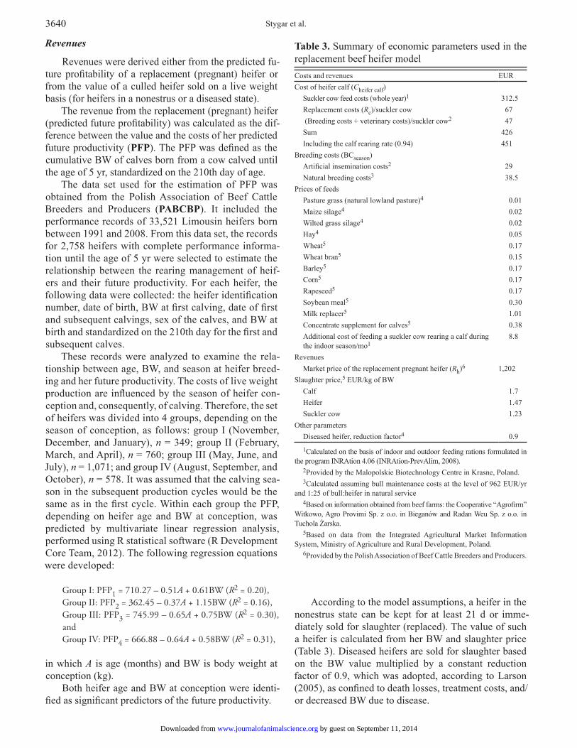
Revenues

Revenues were derived either from the predicted fu-ture profitability of a replacement (pregnant) heifer or from the value of a culled heifer sold on a live weight basis (for heifers in a nonestrus or a diseased state).

The revenue from the replacement (pregnant) heifer (predicted future profitability) was calculated as the dif-ference between the value and the costs of her predicted future productivity (PFP). The PFP was defined as the cumulative BW of calves born from a cow calved until the age of 5 yr, standardized on the 210th day of age.

The data set used for the estimation of PFP was obtained from the Polish Association of Beef Cattle Breeders and Producers (PABCBP). It included the performance records of 33,521 Limousin heifers born between 1991 and 2008. From this data set, the records for 2,758 heifers with complete performance informa-tion until the age of 5 yr were selected to estimate the relationship between the rearing management of heif-ers and their future productivity. For each heifer, the following data were collected: the heifer identification number, date of birth, BW at first calving, date of first and subsequent calvings, sex of the calves, and BW at birth and standardized on the 210th day for the first and subsequent calves.

These records were analyzed to examine the rela-tionship between age, BW, and season at heifer breed-ing and her future productivity. The costs of live weight production are influenced by the season of heifer con-ception and, consequently, of calving. Therefore, the set of heifers was divided into 4 groups, depending on the season of conception, as follows: group I (November, December, and January), n = 349; group II (February, March, and April), n = 760; group III (May, June, and July), n = 1,071; and group IV (August, September, and October), n = 578. It was assumed that the calving sea-son in the subsequent production cycles would be the same as in the first cycle. Within each group the PFP, depending on heifer age and BW at conception, was predicted by multivariate linear regression analysis, performed using R statistical software (R Development Core Team, 2012). The following regression equations were developed:

Group I: PFP1 = 710.27 – 0.51A + 0.61BW (R2 = 0.20),Group II: PFP2 = 362.45 – 0.37A + 1.15BW (R2 = 0.16),Group III: PFP3 = 745.99 – 0.65A + 0.75BW (R2 = 0.30), andGroup IV: PFP4 = 666.88 – 0.64A + 0.58BW (R2 = 0.31),

in which A is age (months) and BW is body weight at conception (kg).

Both heifer age and BW at conception were identi-fied as significant predictors of the future productivity.

According to the model assumptions, a heifer in the nonestrus state can be kept for at least 21 d or imme-diately sold for slaughter (replaced). The value of such a heifer is calculated from her BW and slaughter price (Table 3). Diseased heifers are sold for slaughter based on the BW value multiplied by a constant reduction factor of 0.9, which was adopted, according to Larson (2005), as confined to death losses, treatment costs, and/or decreased BW due to disease.

Table 3. Summary of economic parameters used in the replacement beef heifer modelCosts and revenues EURCost of heifer calf (Cheifer calf)

Suckler cow feed costs (whole year)1 312.5Replacement costs (Rc)/suckler cow 67 (Breeding costs + veterinary costs)/suckler cow2 47Sum 426Including the calf rearing rate (0.94) 451

Breeding costs (BCseason)Artificial insemination costs2 29Natural breeding costs3 38.5

Prices of feedsPasture grass (natural lowland pasture)4 0.01Maize silage4 0.02Wilted grass silage4 0.02Hay4 0.05Wheat5 0.17Wheat bran5 0.15Barley5 0.17Corn5 0.17Rapeseed5 0.17Soybean meal5 0.30Milk replacer5 1.01Concentrate supplement for calves5 0.38Additional cost of feeding a suckler cow rearing a calf during the indoor season/mo1

8.8

RevenuesMarket price of the replacement pregnant heifer (Rh)6 1,202

Slaughter price,5 EUR/kg of BWCalf 1.7Heifer 1.47Suckler cow 1.23

Other parametersDiseased heifer, reduction factor4 0.9

1Calculated on the basis of indoor and outdoor feeding rations formulated in the program INRAtion 4.06 (INRAtion-PrevAlim, 2008).

2Provided by the Malopolskie Biotechnology Centre in Krasne, Poland.3Calculated assuming bull maintenance costs at the level of 962 EUR/yr

and 1:25 of bull:heifer in natural service4Based on information obtained from beef farms: the Cooperative “Agrofirm”

Witkowo, Agro Provimi Sp. z o.o. in Bieganów and Radan Weu Sp. z o.o. in Tuchola Żarska.

5Based on data from the Integrated Agricultural Market Information System, Ministry of Agriculture and Rural Development, Poland.

6Provided by the Polish Association of Beef Cattle Breeders and Producers.




Net Return

The overall net return was calculated as the expected revenue per heifer minus heifer rearing costs, including feed costs, breeding costs, and costs of heifer–calf re-placement. The costs were estimated on the basis of all information available from the stage, state, and decision of child level 2 and both ancestral levels.

The net return in the model was calculated on the basis of an immediate expected reward ( d

ir ) obtained for a specific level ρ1,2 (ρ1 = preweaning period and ρ2 = reproductive period), stage (n), state (i), and the decision (keep, wean, breed, or replace).

For each decision, the expected reward ( dir ) was cal-

culated as follows:

Decision to keep:

( )( )( )

heifer calf preweaning 1

keeppreweaning 1

LP reproductive 2

FC , keep , for 0,

FC , keep , for 1 10,

FC , keep , for

i

C n n

r n n

n

r

r

r

− − == − ≤ <−

,

in which keepir = expected reward for state i and stage

n when the decision is to keep the heifer until the next stage with the defined growth rate; Cheifer calf = cost of the heifer calf calculated as the annual maintenance costs of the suckler cow (including annual feed costs, re-placement costs, and breeding costs + veterinary costs); FC(n, keeppreweaning) = feed costs at stage n, depending on the defined growth rate during the preweaning pe-riod; FCLP(n, keeppreproductive) = feed costs at stage n, calculated in the linear programming submodel, depend-ing on the defined growth rate during the reproductive period; keeppreweaning = the decision to keep in the pre-weaning period with a growth rate of 800 or 1,000 g/d; and keepreproductive = the decision to keep in the repro-ductive period with a growth rate of 400, 600, or 800 g/d.

Decision to wean:

( ) ( )( )

( ) ( ) ( )( ) ( )

heifer calf LPmo 1,2

2wean

LP 2mo 1,2

LP 2

FC FC weaned ,

for 0, weaned

FC FC weaned , for 1, weaned

FC weaned , for 2, weaned

i

C

nr

n

n

r

r

r

− − −

==

− − =− ≥

in which weanir = expected reward for state i and stage n

of the preweaning period when the decision is to wean the heifer with a growth rate of 400, 600, or 800 g/d in the reproductive period; FCmo = feed costs for calves weaned at age <2 mo (If n = 0, FCmo(1,2) is calculated for the first 2 mo of life; if n = 1, only FCmo(2) for the second month of life is included.); and FCLP(weaned) = feed costs in the weaned stage calculated in the lin-ear programming submodel, depending on the defined growth rate (800 or 1,000 g/d) and the duration of the

weaned stage (If n = 0 or n = 1, FCLP(weaned) is calcu-lated for 7 mo; if n ≥ 2, FCLP(weaned) is calculated ac-cording to the duration of the weaned stage [1–7 mo].).

Decision to breed:

( )breedLP season 2FC , breed BC , for ir n r= − − ,

in which breedir = expected reward for state i at stage n

when the decision is to breed a heifer by AI during the indoor season or by NS during the outdoor season and to keep her for at least 21 d with the growth rate of 400, 600, or 800 g/d; FCLP(n, breed) = feed costs at stage n calculated in the linear programming submodel, de-pending on the defined growth rate during reproductive period; and BCseason = breeding costs depending on the season of the year, that is, AI costs in the indoor season and NS costs in the outdoor season.

Decision to replace:

( )( ) ( )

( )

1,2

replace

1,2

2

0.9 LWV , for diseased,

PFP SP PC ,

for pregnant,

LWV , for nonestrus,

r

r

r

i

i ii

i

n

n nr

n

×

× − =

,

in which replaceir immediate expected reward for state i

at stage n and the decision replace calculated from the heifer BW value for heifers in the diseased and nones-trus states or from the predicted future profitability for heifers in the pregnant state; LWVi(n) = live weight val-ue of a heifer in state i at stage n [heifer BW (kg) × price of 1 kg of heifer BW (set equal to the slaughter price)]; PFPi(n) = predicted future productivity (cumulative BW of calves born from a cow calved until the age of 5 yr, standardized on the 210th day of age) for a heifer bred at stage n and in state i; SP = price of 1 kg of calf BW standardized on the 210th day of age (set equal to the slaughter price); and PCi(n) = production costs of 1 kg of calf BW standardized on the 210th day of age for a heifer bred at stage n and in state i.

The Data

The technical and economic input values in the beef heifer model were defined by adopting the mean and limit values estimated on the basis of a literature review and empirical data representing the Limousin cattle pop-ulation in Poland. Information on applied feeding strate-gies, mortality rates, and prices of forages were obtained from the managers of the 3 leading Polish Limousin breeding herds.



Stygar et al.3642

Running the Model in Multilevel Hierarchic Markov Process

The model was programmed in Java as “the beef heif-er” plug-in to the MLHMP software system developed by Kristensen (2003). The plug-in integrates the model struc-ture; transition probabilities; and biological, production, and economic parameters with the MLHMP platform used to compute the optimal policy. The MLHMP platform is a software tool that together with “the beef heifer” plug-in can be freely downloaded from the Internet (www.prod-styr.ihh.kvl.dk/software/mlhmp.html). Through the graphi-cal interface, it allows the user to input and edit the model structure and parameters as well as display the optimal policy together with the value of each decision. Owing to Markov chain simulations in MLHMP software, it is pos-sible to calculate the technical and economic results of op-timal and user-defined nonoptimal policies as well as to check whether the model behaves according to the system specification and compare the model output with the real world data. Therefore, the software also provides an impor-tant tool for internal model validation and verification.

RESULTS AND DISCUSSION

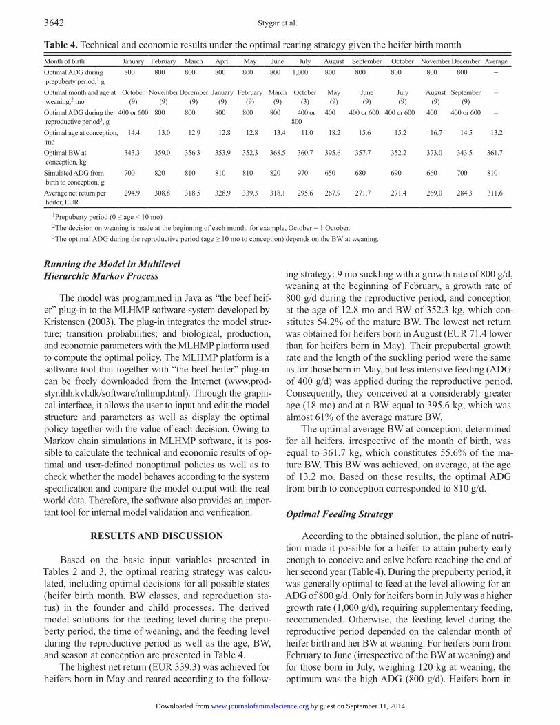
Based on the basic input variables presented in Tables 2 and 3, the optimal rearing strategy was calcu-lated, including optimal decisions for all possible states (heifer birth month, BW classes, and reproduction sta-tus) in the founder and child processes. The derived model solutions for the feeding level during the prepu-berty period, the time of weaning, and the feeding level during the reproductive period as well as the age, BW, and season at conception are presented in Table 4.

The highest net return (EUR 339.3) was achieved for heifers born in May and reared according to the follow-

ing strategy: 9 mo suckling with a growth rate of 800 g/d, weaning at the beginning of February, a growth rate of 800 g/d during the reproductive period, and conception at the age of 12.8 mo and BW of 352.3 kg, which con-stitutes 54.2% of the mature BW. The lowest net return was obtained for heifers born in August (EUR 71.4 lower than for heifers born in May). Their prepubertal growth rate and the length of the suckling period were the same as for those born in May, but less intensive feeding (ADG of 400 g/d) was applied during the reproductive period. Consequently, they conceived at a considerably greater age (18 mo) and at a BW equal to 395.6 kg, which was almost 61% of the average mature BW.

The optimal average BW at conception, determined for all heifers, irrespective of the month of birth, was equal to 361.7 kg, which constitutes 55.6% of the ma-ture BW. This BW was achieved, on average, at the age of 13.2 mo. Based on these results, the optimal ADG from birth to conception corresponded to 810 g/d.

Optimal Feeding Strategy

According to the obtained solution, the plane of nutri-tion made it possible for a heifer to attain puberty early enough to conceive and calve before reaching the end of her second year (Table 4). During the prepuberty period, it was generally optimal to feed at the level allowing for an ADG of 800 g/d. Only for heifers born in July was a higher growth rate (1,000 g/d), requiring supplementary feeding, recommended. Otherwise, the feeding level during the reproductive period depended on the calendar month of heifer birth and her BW at weaning. For heifers born from February to June (irrespective of the BW at weaning) and for those born in July, weighing 120 kg at weaning, the optimum was the high ADG (800 g/d). Heifers born in

Table 4. Technical and economic results under the optimal rearing strategy given the heifer birth monthMonth of birth January February March April May June July August September October November December AverageOptimal ADG during prepuberty period,1 g

800 800 800 800 800 800 1,000 800 800 800 800 800 –

Optimal month and age at weaning,2 mo

October(9)

November(9)

December(9)

January(9)

February(9)

March(9)

October(3)

May(9)

June(9)

July(9)

August(9)

September(9)

–

Optimal ADG during the reproductive period3, g

400 or 600 800 800 800 800 800 400 or 800

400 400 or 600 400 or 600 400 400 or 600 –

Optimal age at conception, mo

14.4 13.0 12.9 12.8 12.8 13.4 11.0 18.2 15.6 15.2 16.7 14.5 13.2

Optimal BW at conception, kg

343.3 359.0 356.3 353.9 352.3 368.5 360.7 395.6 357.7 352.2 373.0 343.5 361.7

Simulated ADG from birth to conception, g

700 820 810 810 810 820 970 650 680 690 660 700 810

Average net return per heifer, EUR

294.9 308.8 318.5 328.9 339.3 318.1 295.6 267.9 271.7 271.4 269.0 284.3 311.6

1Prepuberty period (0 ≤ age < 10 mo)2The decision on weaning is made at the beginning of each month, for example, October = 1 October.3The optimal ADG during the reproductive period (age ≥ 10 mo to conception) depends on the BW at weaning.




the remaining month of the year were fed less intensively, with ADG at the level of 400 or 600 g/d, depending on the weaning weight. For illustrative purposes, the simulated ADG from birth to conception, calculated based on the optimal strategy, is also presented (Table 4).

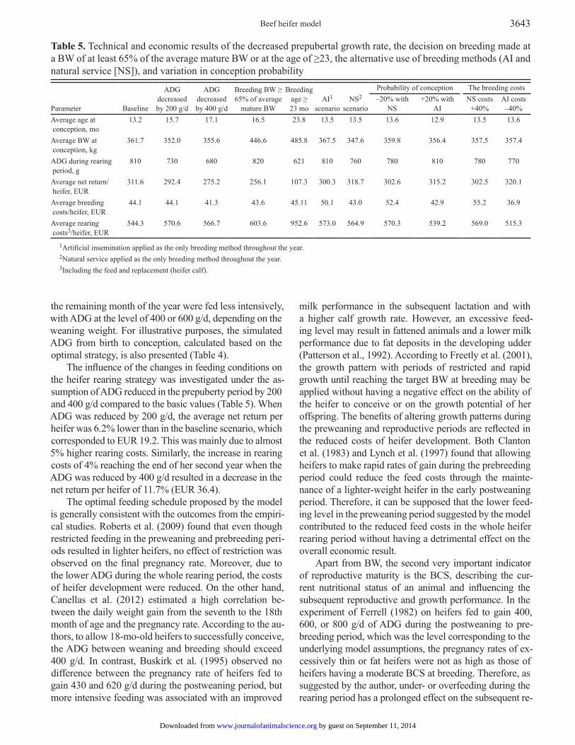
The influence of the changes in feeding conditions on the heifer rearing strategy was investigated under the as-sumption of ADG reduced in the prepuberty period by 200 and 400 g/d compared to the basic values (Table 5). When ADG was reduced by 200 g/d, the average net return per heifer was 6.2% lower than in the baseline scenario, which corresponded to EUR 19.2. This was mainly due to almost 5% higher rearing costs. Similarly, the increase in rearing costs of 4% reaching the end of her second year when the ADG was reduced by 400 g/d resulted in a decrease in the net return per heifer of 11.7% (EUR 36.4).

The optimal feeding schedule proposed by the model is generally consistent with the outcomes from the empiri-cal studies. Roberts et al. (2009) found that even though restricted feeding in the preweaning and prebreeding peri-ods resulted in lighter heifers, no effect of restriction was observed on the final pregnancy rate. Moreover, due to the lower ADG during the whole rearing period, the costs of heifer development were reduced. On the other hand, Canellas et al. (2012) estimated a high correlation be-tween the daily weight gain from the seventh to the 18th month of age and the pregnancy rate. According to the au-thors, to allow 18-mo-old heifers to successfully conceive, the ADG between weaning and breeding should exceed 400 g/d. In contrast, Buskirk et al. (1995) observed no difference between the pregnancy rate of heifers fed to gain 430 and 620 g/d during the postweaning period, but more intensive feeding was associated with an improved

milk performance in the subsequent lactation and with a higher calf growth rate. However, an excessive feed-ing level may result in fattened animals and a lower milk performance due to fat deposits in the developing udder (Patterson et al., 1992). According to Freetly et al. (2001), the growth pattern with periods of restricted and rapid growth until reaching the target BW at breeding may be applied without having a negative effect on the ability of the heifer to conceive or on the growth potential of her offspring. The benefits of altering growth patterns during the preweaning and reproductive periods are reflected in the reduced costs of heifer development. Both Clanton et al. (1983) and Lynch et al. (1997) found that allowing heifers to make rapid rates of gain during the prebreeding period could reduce the feed costs through the mainte-nance of a lighter-weight heifer in the early postweaning period. Therefore, it can be supposed that the lower feed-ing level in the preweaning period suggested by the model contributed to the reduced feed costs in the whole heifer rearing period without having a detrimental effect on the overall economic result.

Apart from BW, the second very important indicator of reproductive maturity is the BCS, describing the cur-rent nutritional status of an animal and influencing the subsequent reproductive and growth performance. In the experiment of Ferrell (1982) on heifers fed to gain 400, 600, or 800 g/d of ADG during the postweaning to pre-breeding period, which was the level corresponding to the underlying model assumptions, the pregnancy rates of ex-cessively thin or fat heifers were not as high as those of heifers having a moderate BCS at breeding. Therefore, as suggested by the author, under- or overfeeding during the rearing period has a prolonged effect on the subsequent re-

Table 5. Technical and economic results of the decreased prepubertal growth rate, the decision on breeding made at a BW of at least 65% of the average mature BW or at the age of ≥23, the alternative use of breeding methods (AI and natural service [NS]), and variation in conception probability

Parameter

Baseline

ADG decreasedby 200 g/d

ADG decreasedby 400 g/d

Breeding BW ≥ 65% of average

mature BW

Breeding age ≥ 23 mo

AI1

scenario

NS2

scenario

Probability of conception The breeding costs–20% with

NS+20% with

AINS costs

+40%AI costs–40%

Average age at conception, mo

13.2 15.7 17.1 16.5 23.8 13.5 13.5 13.6 12.9 13.5 13.6

Average BW at conception, kg

361.7 352.0 355.6 446.6 485.8 367.5 347.6 359.8 356.4 357.5 357.4

ADG during rearing period, g

810 730 680 820 621 810 760 780 810 780 770

Average net return/ heifer, EUR

311.6 292.4 275.2 256.1 107.3 300.3 318.7 302.6 315.2 302.5 320.1

Average breeding costs/heifer, EUR

44.1 44.1 41.3 43.6 45.11 50.1 43.0 52.4 42.9 55.2 36.9

Average rearing costs3/heifer, EUR

544.3 570.6 566.7 603.6 952.6 573.0 564.9 570.3 539.2 569.0 515.3

1Artificial insemination applied as the only breeding method throughout the year.2Natural service applied as the only breeding method throughout the year.3Including the feed and replacement (heifer calf).



Stygar et al.3644

productive performance. However, despite the importance of BCS in heifer breeding management, studies are still lacking on the quantitative relationship of the combination of 3 traits—BW, BW gain, and BCS—with the concep-tion rate. Therefore, the effect of heifer body condition on the probability of conception was not taken into account in the model presented. Similarly, Mourits et al. (1999), who developed a dairy heifer rearing model, pointed out the problem of the scarcity of information on the relation-ship between body condition and BW, growth rate, and the growth pattern. An extension of the model for the evalu-ation of heifer condition might be especially important in determining the effect of possible under- or overfeeding during the reproductive period and, consequently, might contribute to an increase in the accuracy of model solu-tions. However, including such information would prob-ably cause the enlargement of the model to a currently prohibitive size.

Optimal Weaning Strategy

According to the model solution, for most heifers the optimal strategy was to be weaned after a maximum pos-sible suckling time of 9 mo, irrespective of the attained BW and calendar month at birth and at weaning. With late weaning (at the age of 9 mo), the overall costs of heifer rearing were reduced, since suckling is always cheap-er compared with feeding a weaned calf. Weaning at a younger age (3 mo) only proved to be profitable for heifers born in July and was associated with a high ADG (1,000 g/d) from birth to weaning, which allowed the target BW to be reached in the optimal breeding season. The optimal weaning strategy calculated in the model is consistent with the study of Story et al. (2000), who concluded that the calf rearing costs were higher for the early weaned (fifth month of age) than for the normally weaned (seventh month of age) and late-weaned calves (ninth month of age).

An extension of the suckling period contributes to the reduction of rearing costs but can negatively influence the BW and BCS of suckler cows. According to Grings et al. (2005), cows suckled for 240 d weighed less and had a low-er BCS than cows that weaned calves at the age of 190 d. However, the same authors did not observe a difference in the subsequent lactation performance of suckler cows that weaned calves at various ages, ranging from approximately 4.5 to 8 mo. Therefore, ignoring the possible negative ef-fect of a long suckling period on the BW and body condi-tion of a suckler cow seems to be justified in the model.

In the model, the decision on weaning was possible in any calendar month, while in practice, mainly due to orga-nizational reasons, weaning is usually performed at the end of the outdoor season. To illustrate the difference between the optimal results obtained with the base model assump-tions (length of the suckling period 9 mo) and the results of

the weaning strategy generally applied in Polish conditions, a simulation of the weaning of heifers born from March to May at the end of the pasture season (1 November) was per-formed. Weaning at the age of 8 mo (heifers born in March) resulted in only a 1% decrease (EUR 3.1) in the average net return per heifer, while weaning at the age of 6 mo (heifers born in May) caused a 2% reduction in the achieved net re-turn (EUR 6.8). Nevertheless, it should be emphasized that the model assumes that farmers have sufficient facilities to handle the groups of young stock separated or kept with their mothers during both the indoor and outdoor season. The potential additional costs of weaning operations per-formed outside the pasture season were not considered in the model due to the lack of reliable data. Inclusion of these costs might make some of the currently optimal weaning decisions less profitable, all the more so because the dif-ference between the average net return of an optimal and a nonoptimal weaning strategy is small. Therefore, pro-ducers should compare the potential profits achieved from weaning according to the model solution with the potential costs of additional labor and facilities required for weaning during the indoor season.

Optimal Breeding Strategy: Age and Weight at Breeding

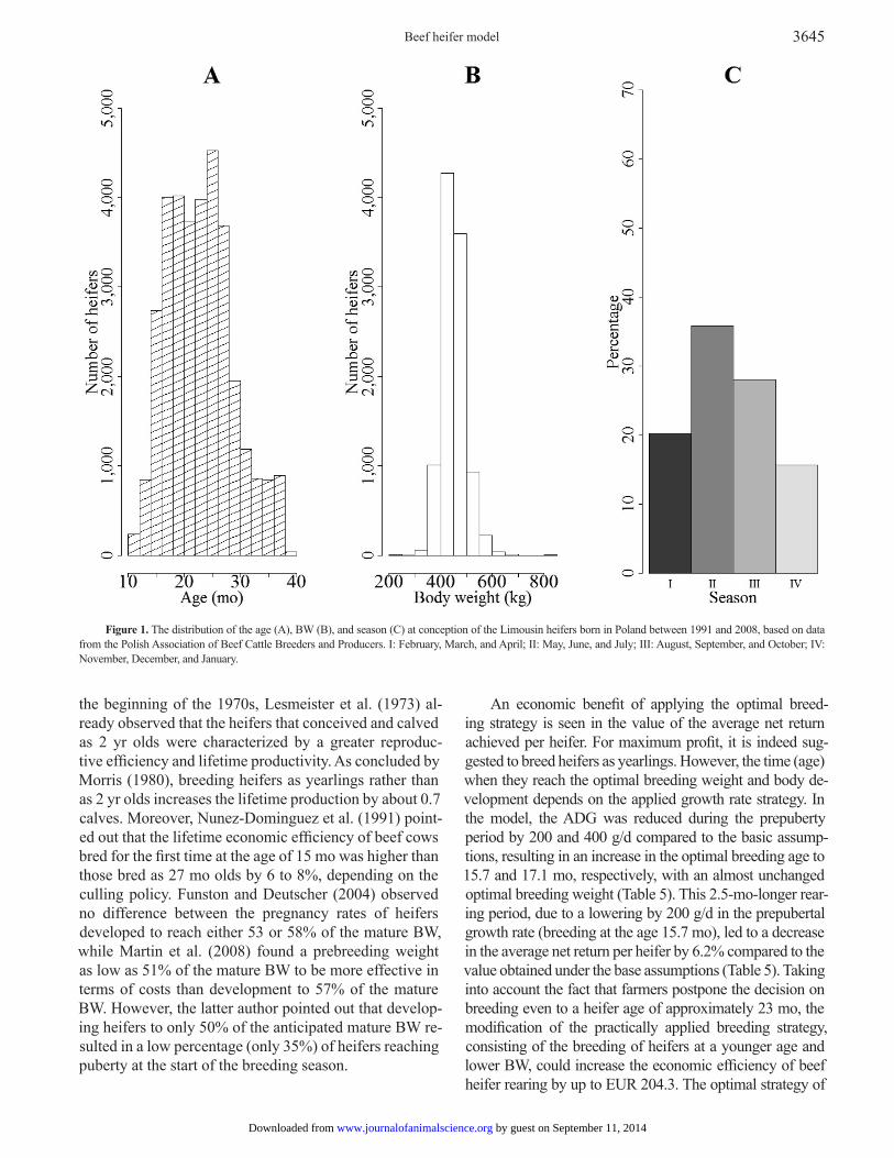
According to the traditional beef production guide-lines, heifers should be bred after reaching 60 to 65% of the mature BW and calve at the age of 2 yr (Patterson et al., 1992). Nevertheless, the analysis of the data from the Polish Limousin population (PABCBP) indicates that both heifer age and BW at breeding were outside the range of conventionally recommended values (Fig. 1). The heifers were bred on average at the age of approximately 23 mo and at the BW equivalent to 70% of the average mature BW. With such an extension of the average rearing period, only 6.5% of heifers conceived by the age of 15 mo. The most likely reason for the postponed decision on breeding is the belief that calving until the age of 2 yr, at a lower BW, unfavorably affects the future growth as well as reproduc-tion and production performance of a heifer.

However, these beliefs are not justified by the model solutions and the information from the reviewed litera-ture. According to the optimal model policy, heifers fed during the whole rearing period at the average level of 810 g/d of ADG should already be bred at the age of 13.2 mo and BW of 361.7 kg, which constitutes 55.6% of the average mature BW, assumed as 650 kg (Table 4). Under the optimum strategy, 76.2% of the heifers conceived before attaining 375 kg of BW and only 5.1% had a BW at conception equal to or higher than 400 kg (Fig. 2).

The obtained results are consistent with previous em-pirical findings indicating not only a lack of worsening but even an improvement in production and the economic effect of the decreased age and BW at heifer breeding. At




the beginning of the 1970s, Lesmeister et al. (1973) al-ready observed that the heifers that conceived and calved as 2 yr olds were characterized by a greater reproduc-tive efficiency and lifetime productivity. As concluded by Morris (1980), breeding heifers as yearlings rather than as 2 yr olds increases the lifetime production by about 0.7 calves. Moreover, Nunez-Dominguez et al. (1991) point-ed out that the lifetime economic efficiency of beef cows bred for the first time at the age of 15 mo was higher than those bred as 27 mo olds by 6 to 8%, depending on the culling policy. Funston and Deutscher (2004) observed no difference between the pregnancy rates of heifers developed to reach either 53 or 58% of the mature BW, while Martin et al. (2008) found a prebreeding weight as low as 51% of the mature BW to be more effective in terms of costs than development to 57% of the mature BW. However, the latter author pointed out that develop-ing heifers to only 50% of the anticipated mature BW re-sulted in a low percentage (only 35%) of heifers reaching puberty at the start of the breeding season.

An economic benefit of applying the optimal breed-ing strategy is seen in the value of the average net return achieved per heifer. For maximum profit, it is indeed sug-gested to breed heifers as yearlings. However, the time (age) when they reach the optimal breeding weight and body de-velopment depends on the applied growth rate strategy. In the model, the ADG was reduced during the prepuberty period by 200 and 400 g/d compared to the basic assump-tions, resulting in an increase in the optimal breeding age to 15.7 and 17.1 mo, respectively, with an almost unchanged optimal breeding weight (Table 5). This 2.5-mo-longer rear-ing period, due to a lowering by 200 g/d in the prepubertal growth rate (breeding at the age 15.7 mo), led to a decrease in the average net return per heifer by 6.2% compared to the value obtained under the base assumptions (Table 5). Taking into account the fact that farmers postpone the decision on breeding even to a heifer age of approximately 23 mo, the modification of the practically applied breeding strategy, consisting of the breeding of heifers at a younger age and lower BW, could increase the economic efficiency of beef heifer rearing by up to EUR 204.3. The optimal strategy of

Figure 1. The distribution of the age (A), BW (B), and season (C) at conception of the Limousin heifers born in Poland between 1991 and 2008, based on data from the Polish Association of Beef Cattle Breeders and Producers. I: February, March, and April; II: May, June, and July; III: August, September, and October; IV: November, December, and January.



Stygar et al.3646

breeding at 55.6% of the average mature BW may result in a growth in the average net return per heifer by almost EUR 55.5 (18%) compared to the conventional system of breed-ing after reaching 65% of the mature BW (Table 5).

Morrison et al. (1992) claimed that heifers exposed to first breeding at the age of 15 mo are lighter and lower and have a smaller pelvic area at calving than those con-ceiving at an older age. Therefore, possible difficulty in calving is the major concern for heifers bred as yearlings. However, this risk can be reduced by selecting sires with a low birth weight among the expected progeny (Colburn et al., 1997) or by better management of heifers during gestation (e.g., appropriate feeding level). In the model, the relationship between age and BW at first breeding and the occurrence of dystocia was indirectly taken into account through the estimation of the PFP for heifers bred at a specific age, BW, and even season of the year.

Empirical studies indicate that the probability of conception increases from the first to the third estrus of a heifer. For example, Byerley et al. (1987) found a con-ception rate for heifers bred during the first estrus of 57% and for those bred during the third estrus of 78%. This increase is associated not only with the hormonal changes but also with body development and reaching physiologi-cal maturity for reproduction. In the model, the increase in the probability of conception does not directly depend on the estrus number but results from the increased BW in the subsequent estrus cycle. The inclusion of the cycle number would probably contribute to a slightly higher accuracy of the optimal solutions but would also signifi-cantly extend the state space of the model (currently it is 1,648,322 states). Moreover, the sensitivity analyses indi-cated that ±20% changes in the probability of conception (due to the application of different breeding methods, i.e., AI and NS) only had a small impact on the average age and BW at conception as well as on the net return per heifer (Table 5). Therefore, it can be supposed that includ-ing the information on the estrus number would have a rather negligible effect on the model outcomes.

Season of Breeding

Under the base model assumptions, for 76.4% of heifers the optimum strategy was to conceive in the out-door season when NS was performed (52% in season 2, from May to July, and 24.4% in season 3, from August to October). The remaining 23.6% of heifers were conceived during the indoor season, when AI was used as a breed-ing method (23% in season 1, from February to April, and 0.6% in season 4, from November to January; Fig. 1).

The breeding season was not sensitive to the varia-tion in rearing conditions, that is, the decrease by 200 or 400 g/d in the prepubertal ADG and the assumed tar-get BW at breeding of 65% of the average mature BW.

These results are generally consistent with the breeding practices applied in the Polish Limousin herds (Fig. 2).

Because of climatic differences influencing manage-ment practices, it is difficult to compare the seasonality of breeding in separate geographic regions of the world. Surprisingly, however, similar findings on the optimal breeding season in beef herds maintained in the range-lands of the northern Great Plains (of the United States) were described by Grings et al. (2005), who also report-ed a higher weaning weight of calves born in late win-ter (February) and spring (April) than of calves born in early summer (June). This observation was confirmed in the dynamic model simulations performed by Reisenauer Leesburg et al. (2007), which indicated that switching from early spring to summer or fall calvings was not ex-pected to improve the profitability of cow–calf operations.

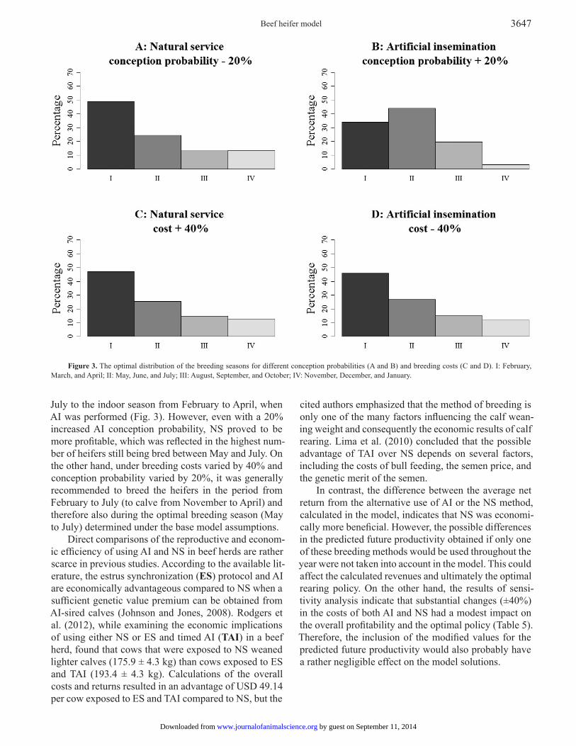
As occurs in practice, the model assumed seasonal-ity in the method of breeding: AI in the indoor season and NS in the outdoor (pasture) season. Since the out-door season includes the months determined as optimal for breeding, one may suspect that the choice of breed-ing method could also affect the obtained solution. This is all the more so because the assumption of applying only 1 method of breeding throughout the year, either AI or NS, affected the optimal distribution of breeding seasons. This could be justified by the different costs and the probability of conception in each of these meth-ods. The obtained results indicate that a 40% increase in the NS cost or a 40% decrease in the AI cost (with the conception probability unchanged in both cases) as well as a 20% decrease in the NS conception probability (with the unchanged cost of breeding) compared to base model assumptions caused a shift in the highest number of breedings from the outdoor season between May and

Figure 2. The distribution of heifer BW (A) and season at conception (B) under the optimal rearing strategy. I: February, March, and April; II: May, June, and July; III: August, September, and October; IV: November, December, and January.




July to the indoor season from February to April, when AI was performed (Fig. 3). However, even with a 20% increased AI conception probability, NS proved to be more profitable, which was reflected in the highest num-ber of heifers still being bred between May and July. On the other hand, under breeding costs varied by 40% and conception probability varied by 20%, it was generally recommended to breed the heifers in the period from February to July (to calve from November to April) and therefore also during the optimal breeding season (May to July) determined under the base model assumptions.

Direct comparisons of the reproductive and econom-ic efficiency of using AI and NS in beef herds are rather scarce in previous studies. According to the available lit-erature, the estrus synchronization (ES) protocol and AI are economically advantageous compared to NS when a sufficient genetic value premium can be obtained from AI-sired calves (Johnson and Jones, 2008). Rodgers et al. (2012), while examining the economic implications of using either NS or ES and timed AI (TAI) in a beef herd, found that cows that were exposed to NS weaned lighter calves (175.9 ± 4.3 kg) than cows exposed to ES and TAI (193.4 ± 4.3 kg). Calculations of the overall costs and returns resulted in an advantage of USD 49.14 per cow exposed to ES and TAI compared to NS, but the

cited authors emphasized that the method of breeding is only one of the many factors influencing the calf wean-ing weight and consequently the economic results of calf rearing. Lima et al. (2010) concluded that the possible advantage of TAI over NS depends on several factors, including the costs of bull feeding, the semen price, and the genetic merit of the semen.

In contrast, the difference between the average net return from the alternative use of AI or the NS method, calculated in the model, indicates that NS was economi-cally more beneficial. However, the possible differences in the predicted future productivity obtained if only one of these breeding methods would be used throughout the year were not taken into account in the model. This could affect the calculated revenues and ultimately the optimal rearing policy. On the other hand, the results of sensi-tivity analysis indicate that substantial changes (±40%) in the costs of both AI and NS had a modest impact on the overall profitability and the optimal policy (Table 5). Therefore, the inclusion of the modified values for the predicted future productivity would also probably have a rather negligible effect on the model solutions.

Figure 3. The optimal distribution of the breeding seasons for different conception probabilities (A and B) and breeding costs (C and D). I: February, March, and April; II: May, June, and July; III: August, September, and October; IV: November, December, and January.



Stygar et al.3648

Applicability of the Model

To the best knowledge of the authors, the presented model is the first application of MLHMP in determining the economically optimal rearing strategies for replace-ment beef heifers. Due to the probabilistic Markov chain simulations in the MLHMP software, the model can also calculate the technical and economic key figures charac-terizing the optimal and user-defined nonoptimal rear-ing policies. It handles large sets of situations and facts that can occur in the real world. Taking into account the biological variation within the population, it fulfills the postulate of Shafer et al. (2007), who concluded, based on the example of the Colorado cow–calf production model, that simulating realistic levels of variability must be an integral part of model development. Similarly to the approach of Kristensen (1987) used in a dairy cow model, computing the expected extra profit from breed-ing a heifer in the present state, compared with postpon-ing the breeding decision by 21 d, allows the ranking of individual heifer breeding decisions. However, over 1,600,000 states and the several decisions made on 3 lev-els of the hierarchic structure of the model made it im-possible to present in this paper the whole optimal rear-ing policy, apart from the summarized average results for each birth month of the heifer.

By changing the key variables and parameters, the model allows testing of the economically optimal man-agement strategy for various beef heifer breeds under dif-ferent technical and economic conditions. Due to the pos-sibility of taking into account the conditions of an individ-ual farm, it can be used as a decision support tool for beef producers and agricultural advisors. However, although the model is suitable for use on the farm level, some its recommendations may be too complex and it may there-fore appear to be too difficult to fully apply in practice (e.g., the optimal feeding and weaning policy differs for 2 consecutive heifer birth months: June and July).

Apart from supplying exact figures, the replacement beef heifer model may serve as an efficient tool to gain insights into the rearing process and, in the future, might also be extended to investigate additional aspects of beef heifer development. The model could also be used to examine the environmental impact (e.g., greenhouse gas [GHG] emissions) of various heifer management deci-sions, mainly including feeding. For this purpose, the output component of the model should be redefined and divided into 2 parts, the net return and GHG emissions from heifer rearing, while the input should be supple-mented by information on fixed GHG emission rates as-sociated with using various feedstuffs in heifer diets.

LITERATURE CITEDAllan, M. F. 2005. Improving feed efficiency through genetics. In:

Proceedings of The Range Beef Cow Symposium XIX December 6, 7 and 8, 2005, Rapid City, South Dakota. p. 33.

Buskirk, D. D., D. B. Faulkner, and F. A. Ireland. 1995. Increased postweaning gain of beef heifers enhances fertility and milk production. J. Anim. Sci. 734:937–946.

Byerley, D. J., R. B. Staigmiller, J. G. Berardinelli, and R. E. Short. 1987. Pregnancy rates of beef heifers bred either on pubertal or third estrus. J. Anim. Sci. 65:645–650.

Canellas, L. C., J. O. J. Barcellos, L. N. Nunes, T. E. de Oliveira, E. R. Prates, and D. C. Darde. 2012. Post-weaning weight gain and pregnancy rate of beef heifers bred at 18 months of age: A meta-analysis approach. R. Bras. Zootec. 41(7):1632–1637.

Clanton, D. C., L. E. Jones, and M. E. England. 1983. Effect of rate and time of gain after weaning on the development of replace-ment beef heifers. J. Anim. Sci. 56:280–285.

Colburn, D. J., G. H. Deutscher, M. K. Nielsen, and D. C. Adams. 1997. Effects of sire, dam traits, calf traits, and environment on dystocia and subsequent reproduction of two-year-old heifers. J. Anim. Sci. 75:1452–1460.

Ferrell, C. L. 1982. Effects of postweaning rate of gain on onset of puberty and productive performance of heifers of different breeds. J. Anim. Sci. 55:1272–1283.

Freetly, H. C., C. L. Ferrell, and T. G. Jenkins. 2001. Production per-formance of beef cows raised on three different nutritionally con-trolled heifer development programs. J. Anim. Sci. 79:819–826.

Funston, R. N., and G. H. Deutscher. 2004. Comparison of target breeding weight and breeding date for replacement beef heifers and effects on subsequent reproduction and calf performance. J. Anim. Sci. 82:3094–3099.

Grings, E. E., R. E. Short, K. D. Klement, T. W. Geary, M. D. MacNeil, and M. R. Haferkamp. 2005. Calving system and weaning age effects on cow and preweaning calf performance in the northern Great Plains J. Anim. Sci. 83:2671–2683.

Healy, V. M., G. W. Boyd, P. H. Gutierrez, R. G. Mortimer, and J. R. Piotrowski. 1993. Investigating optimal bull:heifer ratios re-quired for estrus-synchronized heifers. J. Anim. Sci. 71:291–297.

INRA. 1989. Ruminant nutrition. Recommended allowances and feed tables. John Libbey Eurotext, Paris, France.

INRAtion-PrevAlim. 2008. Computer software ver. 4,06. INRA Theix & Educagri Editions. Bp 87999 F 21079 Dijon Cedex. France.

Johnson, S. K., and R. D. Jones. 2008. A stochastic model to compare breeding system costs for synchronization of estrus and artificial insemination to natural service. Prof. Anim. Sci. 24:588–595.

Kristensen, A. R. 1987. Optimal replacement and ranking of dairy cows determined by a hierarchic Markov process. Livest. Prod. Sci. 16:131–144.

Kristensen, A. R. 2003. A general software system for Markov de-cision processes in herd management applications. Comput. Electron. Agric. 38:199–215.

Kristensen, A. R., and E. Jørgensen. 2000. Multi-level hierarchic Markov processes as a framework for herd management sup-port. Ann. Oper. Res. 94:69–89.

Larson, R. L. 2005. Effect of cattle disease on carcass traits. J. Anim. Sci. 83(Suppl.):E37–E43.

Lesmeister, J. L., P. J. Burfening, and R. L. Blackwell. 1973. Date of first calving in beef cows and subsequent beef production. J. Anim. Sci. 36:1–6.

Lima, F. S., A. De Vries, C. A. Risco, J. E. P. Santos, and W. W. Thatcher. 2010. Economic comparison of natural service and timed artificial insemination breeding programs in dairy cattle. J. Dairy Sci. 93:4404–4413.




Lynch, J. M., G. C. Lamb, B. L. Miller, R. T. Brandt Jr., R. C. Cochran, and J. E. Minton. 1997. Influence of timing of gain on growth and reproductive performance of beef replacement heifers. J. Anim. Sci. 75:1715–1722.

Martin, J. L., K. W. Creighton, J. A. Musgrave, T. J. Klopfenstein, R. T. Clark, D. C. Adams, and R. N. Funston. 2008. Effect of pre-breeding body weight or progestin exposure before breeding on beef heifer performance through the second breeding season. J. Anim. Sci. 86:451–459.

Meaker, H. J. 1984. Effective extensive beef production as a prelude to feedlotting. S. Afr. J. Anim. Sci. 14:158–163.

Morris, G. A. 1980. A review of relationships between aspects of reproduction in beef heifers and their lifetime production. Associations with fertility in the first joining season and with age at first joining. Anim. Breed. Abstr. 48:655–676.

Morrison, D. G., J. I. Feazel, C. P. Bagley, and D. C. Blouin. 1992. Postweaning growth and reproduction of beef heifers exposed to calve at 24 or 30 months of age in spring and fall seasons. J. Anim. Sci. 70:622–630.

Mourits, M. C. M. 2000a. Economic modelling to optimize dairy heifer management decisions. PhD Diss., Wageningen University, The Netherlands.

Mourits, M. C. M., D. T. Galligan, A. A. Dijkhuizen, and R. B. M. Huirne. 2000b. Optimization of dairy heifer management decisions based on production conditions of Pennsylvania. J. Dairy Sci. 83:1989–1997.

Mourits, M. C. M., R. B. M. Huirne, A. A. Dijkhuizen, A. R. Kristensen, and D. T. Galligan. 1999. Economic optimization of dairy heifer management decisions. Agric. Sys. 61:17–31.

Norris, J. R. 1998. Markov chains. Cambridge series in statistical and probabilistic mathematics. Cambridge Univ. Press, Cambridge, UK.

Nunez-Dominguez, R., L. V. Cunfiff, K. E. Dickerson, K. E. Gregory, and R. M. Koch. 1991. Lifetime production of beef heifers calv-ing first at two vs. three years of age. J. Anim. Sci. 69:3467–3479.

Patterson, D. J., R. C. Perry, G. H. Kiracofe, R. A. Bellows, R. B. Staigmiller, and L. R. Corah. 1992. Management considerations in heifer development and puberty. J. Anim. Sci. 70:4018–4035.

Pilarczyk, R., and J. Wójcik. 2007. Comparison of calf rearing re-sults and nursing cow performance in various beef breeds man-aged under the same conditions in north-western Poland. Czech J. Anim. Sci. 52(10):325–333.

R Development Core Team. 2012. R: A language and environment for statistical computing. R Foundation for Statistical Computing, Vienna, Austria.

Reisenauer Leesburg, V. L., M. W. Tess, and D. Griffith. 2007. Evaluation of calving seasons and marketing strategies in Northern Great Plains beef enterprises: I. Cow-calf systems. J. Anim. Sci. 85:2314–2321.

Roberts, A. J., T. W. Geary, E. E. Grings, R. C. Waterman, and M. D. MacNeil. 2009. Reproductive performance of heifers offered ad libitum or restricted access to feed for a one hundred forty-day period after weaning. J. Anim. Sci. 87:3043–3052.

Rodgers, J. C., S. L. Bird , J. E. Larson , N. DiLorenzo , C. R. Dahlen, A. DiCostanzo, and G. Lamb. 2012. An economic evaluation of estrous synchronization and timed artificial insemination in suckled beef cows. J. Anim. Sci., 90:4055-4062.

Shafer, W. R., R. M. Bourdon, and R. M. Enns. 2007. Simulation of cow-calf production with and without realistic levels of vari-ability. J. Anim. Sci. 85:332–340.

Story, C. E., R. J. Rasby, R. T. Clark, and C. T. Milton. 2000. Age of calf at weaning of spring-calving beef cows and the effect on cow and calf performance and production economics. J. Anim. Sci. 78:1403–1413.

Stygar, A. H., and J. Makulska. 2010. Application of mathematical modelling in beef herd management – A review. Ann. Anim. Sci. 10(4):333–348.



Referenceshttp://www.journalofanimalscience.org/content/92/8/3636#BIBLThis article cites 33 articles, 20 of which you can access for free at:


http://www.journalofanimalscience.org/content/92/8/3636#BIBL


Optimal management of replacement heifers in a beef herd: A model for simultaneous optimization of rearing and breeding decisions

Documents