Optimal Intertemporal Pricing ... - curve. · PDF fileThe firm does better by pricing a straightforward new product at a lower introductory price when the product is quite visible

Optimal Intertemporal Pricing Strategies

for Firms Introducing New Products

By

Briana Brownell

A thesis submitted to the Faculty of Graduate and Postdoctoral Affairs

in partial fulfillment of the requirements for the degree of

Master of Arts

in

Economics

Carleton University

Ottawa, Ontario

2014

Briana Brownell

ii

ABSTRACT

Firms can significantly improve their performance upon the introduction of a new product by

following an intertemporal pricing strategy which predicts the adoption of the product

through time. Four reasons for gradual adoption are explored: delayed purchase, awareness,

social pressures and informational needs. The firm does better by pricing a straightforward

new product at a lower introductory price when the product is quite visible to other potential

adopters when an individual adopts. Differences in price-sensitivity among consumers also

impact the firm’s optimal strategy. Products for which the social relevance varies

considerably or for which the average perceived social risk of adoption is high cannot

necessarily benefit from a low introductory price. A high initial price which decreases through

time is better when consumers are varied in their need for information, when on average,

much information is needed and when the information generated by other adopters is

forgotten more quickly.

iii

TABLE OF CONTENTS

ABSTRACT ................................................................................................................................................ II

List of Tables ....................................................................................................................... viii

List of Illustrations ................................................................................................................ ix

List of Appendices ................................................................................................................ xi

CHAPTER 1: OVERVIEW OF DIFFUSION MODELLING ................................................................ 1

1.1 Background and Motivation ............................................................................................. 1

1.2 Relevance for Firms ......................................................................................................... 3

1.3 Behaviour of Consumers .................................................................................................. 5

1.4 Method of Analysis .......................................................................................................... 8

CHAPTER 2: MODEL SET-UP ............................................................................................................ 12

2.1 Description of the Good and Market .............................................................................. 12

2.2 Consumers’ Decisions .................................................................................................... 13

2.2.1 Evolution of Price-Dependent Demand ............................................................................ 14

2.2.2 Heterogeneity of Agents................................................................................................... 17

2.2.3 Valuation of the Good ...................................................................................................... 19

iv

2.2.4 Adoption-associated demand .......................................................................................... 22

2.2.5 Aggregation of Demand .................................................................................................... 24

2.3 Behaviour of Firms ......................................................................................................... 24

2.3.1 Costs of Production .......................................................................................................... 27

2.3.2 Feasibility of Results ......................................................................................................... 29

2.3.3 Competition ...................................................................................................................... 29

2.4 Market Size, Full Adoption, and Underadoption ............................................................. 31

CHAPTER 3: DELAYED PURCHASE ................................................................................................. 32

3.1 Diffusion Due to Delayed Purchase ................................................................................ 32

3.2 Model Framework ......................................................................................................... 32

3.3 Optimization Results ...................................................................................................... 34

3.3.1 Summary of Key Results ................................................................................................... 34

3.3.2 Pricing Strategy ................................................................................................................. 36

3.3.3 Effect of Foresight ............................................................................................................ 37

3.3.4 Effect of Heterogeneity .................................................................................................... 42

3.4 Conclusions ................................................................................................................... 44

CHAPTER 4: DIFFUSION BY AWARENESS .................................................................................... 46

4.1 Awareness as a Diffusion Mechanism ............................................................................. 46

v

4.2 Model Framework ......................................................................................................... 48




4.3.3 Effect of the Diffusion Mechanism ................................................................................... 58



4.4 Conclusions ................................................................................................................... 69

CHAPTER 5: DIFFUSION BY SOCIAL INFLUENCE ....................................................................... 73

5.1 Social Influence as a Diffusion Mechanism ..................................................................... 73

5.2 Model Framework ......................................................................................................... 74

5.2.1 Heterogeneity ................................................................................................................... 76

5.2.2 Constraints on Production ................................................................................................ 77



5.3.1.1 Characterization of the Market Potential .................................................................. 80

5.3.1.2 Pricing Constraints ..................................................................................................... 82

5.3.1.3 The General Case........................................................................................................ 83

5.3.1.4 Normal Distribution.................................................................................................... 84

vi

5.3.1.5 Uniformly Distributed Thresholds .............................................................................. 85


5.3.2.1 Uniformly Distributed Thresholds .............................................................................. 87

5.3.2.2 Normally Distributed Thresholds ............................................................................... 90

5.3.3 Effect of the Diffusion Mechanism ................................................................................... 95



5.4 Conclusions ................................................................................................................. 101

CHAPTER 6: DIFFUSION BY INFORMATION ............................................................................ 104

6.1 Value Uncertainty as a Diffusion Mechanism ................................................................ 104

6.2 Model Framework ....................................................................................................... 106

6.2.1 Heterogeneity ................................................................................................................. 108

6.2.2 Constraint on Production ............................................................................................... 109

6.2.3 Information Generation ................................................................................................. 109

6.3 Optimization Results .................................................................................................... 110

6.3.1 Summary of Key Results ................................................................................................. 110

6.3.1.1 Optimal Solutions of the Continuous Information Generation Model .................... 113

6.3.2 Pricing Strategy ............................................................................................................... 114

6.3.2.1 Normally Distributed Information Requirements .................................................... 115

6.3.3 Information Loss ............................................................................................................. 117

vii

6.3.4 Effect of the Diffusion Mechanism ................................................................................. 120

6.3.5 Effect of Foresight .......................................................................................................... 121

6.3.6 Effect of Heterogeneity .................................................................................................. 123

6.4 Conclusions ................................................................................................................. 124

REFERENCES ....................................................................................................................................... 128

APPENDICES ....................................................................................................................................... 134

viii

List of Tables

Table 1: Lavidge and Steiner’s Model for New Product Adoption .............................................. 6

Table 2: Optimal Solutions for the Purchase Delay Model ....................................................... 36

Table 3: Effect of Foresight on Production Levels ..................................................................... 39

Table 4: Effect of Foresight on Optimal Price............................................................................. 40

Table 5: Optimal Solutions for the Diffusion by Awareness Model .......................................... 53

Table 6: Effect of the Diffusion Mechanism on Optimal Production ........................................ 58

Table 7: Effect of the Diffusion Mechanism on Optimal Price .................................................. 60

Table 8: Effect of Foresight on Optimal Production Level and Price ........................................ 61

Table 9: General Form of the Optimal Solutions for the Diffusion by Conformity Model ........ 83

Table 10: Optimal Solutions for Normally Distributed Thresholds ........................................... 85

Table 11: Optimal Solutions for Uniformly Distributed Thresholds .......................................... 86

Table 12: Effect of the Diffusion Mechanism on Optimal Production Levels .......................... 96

Table 13: Effect of Foresight on Optimal Production Levels ..................................................... 97

Table 14: Effect of Foresight on Optimal Price .......................................................................... 98

Table 15: Optimal Solutions for the Continuous Information Generation Model ................. 114

Table 16: Effect of the Diffusion Mechanism on Optimal Production and Price .................. 121

Table 17: Effect of Foresight on Optimal Production and Price ............................................. 122

ix

List of Illustrations

Figure 1: Optimal Solution for the Eight-Period Problem .......................................................... 35

Figure 2: Optimal Pricing Strategy for the Eight-Period Problem .............................................. 37

Figure 3: Effect of Foresight on Production Per Period and Total Adoption............................. 38

Figure 4: Effect of Foresight on Production Levels .................................................................... 39

Figure 5: Effect of Foresight on the Optimal Pricing Strategy ................................................... 41

Figure 6: Effect of Foresight on Profit ......................................................................................... 42

Figure 7: Effect of Heterogeneity on Price.................................................................................. 43

Figure 8: Price for Various Levels of Heterogeneity ................................................................... 44

Figure 9: Optimal Eight-Period Solution for .................................................... 50

Figure 10: Optimal Eight-Period Solution for .................................................. 51

Figure 11: Optimal Eight-Period Solution for ................................................ 52

Figure 12: Pricing Strategy for Various Parameter Pairs ........................................................... 54

Figure 13: Price and Adoption for Various Parameter Pairs ..................................................... 55

Figure 14: Two Period Pricing Strategy ....................................................................................... 57

Figure 15: Effect of the Diffusion Mechanism on Production and Adoption ........................... 59

Figure 16: Effect of the Diffusion Mechanism on Price and Adoption ..................................... 60

Figure 17: Effect of Heterogeneity on the Optimal Price Policy ................................................ 62

Figure 18: Optimal Price for Various Levels of Heterogeneity .................................................. 63

Figure 19: Curvature Effect ......................................................................................................... 66

Figure 20: Pricing Strategy Boundary for Various Levels of Heterogeneity ............................. 67

Figure 21: Pricing Strategy Regions in the Presence of Heterogenity ...................................... 69

Figure 22: Optimal Eight-Period Solution for Uniformly Distributed Thresholds (1) ................ 78

Figure 23: Optimal Eight-Period Solution for Uniformly Distributed Thresholds (2) ................ 78

x

Figure 24: Optimal Eight-Period Solution for Normally Distributed Thresholds ....................... 79

Figure 25: Illustration of a Distribution of Thresholds with a Fixed Point ................................ 80

Figure 26: Optimal Production for a Distribution of Thresholds with a Fixed Point ................ 81

Figure 27: Illustration of the Production Constraint .................................................................. 83

Figure 28: CDF of Thresholds and Optimal Price Strategy when - ................................ 88

Figure 29: CDF of Thresholds and Optimal Price Strategy when - ................................ 89

Figure 30: CDF of Thresholds and Optimal Price Strategy when ................................... 90

Figure 31: Two Period Pricing Strategy ....................................................................................... 92

Figure 32: Pricing Strategy for the Two Period Case ................................................................. 95

Figure 33: Effect of Foresight on Production Levels.................................................................. 98

Figure 34: Effect of Foresight on Profit ...................................................................................... 99

Figure 35: Effect of Heterogeneity on Price ............................................................................ 100

Figure 36: Optimal Eight-Period Solution for N(0.2,0.2) ........................................................ 111

Figure 37: Optimal Eight-Period Solution for N(0,0.2) ............................................................ 112

Figure 38: Optimal Eight-Period Solution for N(-0.2,0.2) ....................................................... 113

Figure 39: Optimal Pricing Strategy for ...................................................................... 116

Figure 40: Effect of Information Loss on Optimal Price and Production ............................... 118

Figure 41: Optimal Pricing Strategy Boundaries for ................................................. 119

Figure 42: Profit Levels for Various Degrees of Information Loss ......................................... 120

Figure 43: Effect of Foresight on Profit ................................................................................... 123

Figure 44: Effect of Heterogeneity on Price Strategy ............................................................. 124

xi

List of Appendices

A3 APPENDIX TO CHAPTER 3 ....................................................................................................... 134

A3.1 The Two-Period Case ....................................................................................................... 134

A3.1.1 Derivation of the Two Period Full Optimization ....................................................... 134

A3.1.2 Derivation of the Pricing Strategy ............................................................................. 135

A3.1.3 Derivation of the Two Period Static Optimization .................................................... 135

A3.2 The Eight-Period Case ..................................................................................................... 137

A3.2.1 Numeric Solution ...................................................................................................... 139

A3.3 The T-Period Case ............................................................................................................ 140

A3.3.1 Derivation of Optimal Production and Price over T Periods .................................... 140

A3.3.2 Derivation of the Optimal Pricing Strategy ............................................................... 141

A3.3.1.1 Homogeneity ...................................................................................................... 141

A3.3.1.2 Heterogeneity ..................................................................................................... 142

A3.3.3 Derivation of the Static Optimization Solutions ....................................................... 142

A4 Appendix to Chapter 4 .................................................................................................. 144


A4.1.1 Derivation of the Two Period Full Optimization ....................................................... 144

A4.1.1.1 Homogeneity ...................................................................................................... 144

A4.1.1.2 Heterogeneity ..................................................................................................... 147


A4.1.2.1 Homogeneity ...................................................................................................... 150

xii

A4.1.2.2 Heterogeneity ..................................................................................................... 151

A4.1.3 Two-Period Static Optimization ................................................................................ 155


A4.2.1 Numeric Solutions for Various Parameter Pairs ....................................................... 161


A4.3.1 Derivation of the Optimal Production and Price Over T Periods .............................. 164


A4.3.2.1 Homogeneity ...................................................................................................... 166

A4.3.2.2 Heterogeneity ..................................................................................................... 167




A5.1.1 Derivation of the Two-Period Full Optimization ....................................................... 169

A5.1.1.1 Normally Distributed Thresholds ....................................................................... 170





A5.2.1 Numeric Solutions for Various Distributions ............................................................ 178


A5.3.1 Derivation of the Optimal Production and Price over T Periods .............................. 180

A5.3.1.1 Homogeneity ...................................................................................................... 180

xiii

A5.3.1.2 Heterogeneity ..................................................................................................... 182


A5.3.1.4 Uniformly Distributed Thresholds ...................................................................... 184


A5.3.2.1 Homogeneity ...................................................................................................... 185

A5.3.2.2 Heterogeneity ..................................................................................................... 186


A5.3.2.4 Uniformly Distributed Thresholds ...................................................................... 188



A6.1 The Three-Period Case .................................................................................................... 191

A6.1.1 Derivation of the Three-Period Full Optimization—Complete Decay ...................... 191

A6.1.2 Derivation of the Three-Period Full Optimization—No Decay ................................. 193


A6.2.1 Numeric Solutions for Various Distributions ............................................................ 199

A6.2.2 Numeric Solutions for Various Rates of Information Decay ..................................... 201


A6.3.1 Derivation of the Optimal Production and Price over T Periods .............................. 202

A6.3.1.1 Homogeneity ...................................................................................................... 203

A6.3.1.2 Heterogeneity ..................................................................................................... 204

A6.3.2 Derivation of the Price Strategy ................................................................................ 205

A6.3.2.1 Homogeneity ...................................................................................................... 205

xiv

A6.3.2.2 Heterogeneity ..................................................................................................... 206

A6.3.2.3 Normally Distributed Informational Needs ........................................................ 206


1

CHAPTER 1: OVERVIEW OF DIFFUSION MODELLING

1.1 Background and Motivation

The diffusion of new innovations has received considerable attention due to its relevance

across disciplines. Because of its importance in various areas of marketing, sociology, and

economics, each field has formulated a series of sophisticated models using fundamentally

different mechanisms with which to model diffusion. These models are particularly

applicable to a firm introducing a new product in the marketplace that aims to maximize

profit over time knowing that the new product will be adopted by consumers gradually rather

than all at once. A firm that anticipates the diffusion of their product according to a

theoretical model can partially control the adoption of the innovation by altering its price

over time. The present thesis examines the firm’s intertemporal pricing strategy for four

different classes of products.

The theoretical analysis herein is motivated by several stylized facts about how new

products diffuse through the potential adopter population. These generalizations can be

used to inform a firm’s pricing strategy.

Adoption is gradual even if the new product is a clear improvement over the status

quo.

Market-wide adoption of a new product consists of a period of slow adoption followed

by a sharp take-off, which yields the familiar s-shaped adoption curve.

Although the shape of the adoption curve is similar for many different products, there

are notable differences in the shape of some adoption curves.

2

The shape of the general adoption curve often fits despite the effect of firm decision

variables such as price or advertising expenditure.

The diffusion of new products is difficult to predict. They often diffuse more slowly or

to a much lesser extent than anticipated by firms and researchers or, alternatively,

take off suddenly and unexpectedly.

Gradual adoption of innovations is noted by Rogers (1983) as one of the four crucial

components of diffusion research: “The inclusion of time as a variable in diffusion research

is one of its strengths.” (Rogers, 1983, pp. 20). This gradual adoption presents a unique

opportunity to the firm as it can use the knowledge of how a new product diffuses to

improve its long-run performance. The reasons why consumers tend to adopt gradually has

been an area of significant inquiry in various disciplines. Numerous reasons such as loss

aversion, conformity to the status quo, uncertainty, lack of awareness, psychological costs of

behaviour changes, and network effects have been advanced (Granovetter, 1978; Bagwell

and Riordan, 1991; Gourville and Soman, 2002; Nelson et al., 2004; Gourville, 2006;

Navarro, 2012).

Innovations, even in the form of new products, differ greatly. Although empirical studies

have found a similar S-shaped adoption curve for various product categories across

geographic regions and time frames (e.g.: Ryan and Gross, 1943; Horsky, 1990; Bass et al.,

1994), dissimilarities in the early stages of adoption imply that there are likely to be

different underlying mechanisms at work. A certain quality may be much more relevant in

the modeling of one product as compared to another. As Rogers (1983) notes:

3

It should not be assumed, as sometimes has been done in the past, that all

innovations are equivalent units of analysis. This is a gross over-simplification.

While it may take consumer innovations like blue jeans or pocket calculators

only five or six years to reach widespread adoption in the United States, other

new ideas such as the metric system or using seat belts in cars may require

several decades to reach complete use. The characteristics of innovations, as

perceived by individuals, help to explain their different rate of adoption (Rogers,

1983, pp. 15–16).

Young (2009) observes that the diffusion mechanisms studied by various disciplines differ

fundamentally: “Each model leaves a distinctive ‘footprint’ in its pattern of acceleration that

holds with few or no restrictions on the distribution characteristics. The reason is that they

have fundamentally different structures that details in the underlying distributions cannot

overcome” (Young, 2009, pp. 1899–1900). Because of the diversity of new products that

may be considered, four different models are advanced in the present thesis. Each diffusion

model applies to a different class of products that a firm may wish to introduce, depending

on the factors that are relevant to its adoption.

1.2 Relevance for Firms

For firms, the introduction of new products presents a significant opportunity. As Chao et al.

(2012) observe: “Firms believe that continual introduction of new products is an important

aspect of their business and will help attract more demand and maintain a competitive

position in a market” (Chao et al., 2012, p. 211). In a competitive environment, firms are

able to capture monopoly rents upon the introduction of a new product if competitors must

4

take time to develop or copycat the new product. However the risk is high: “New products

fail at the stunning rate of between 40% and 90%, depending on the category” (Gourville,

2006, p. 100).

Pricing a new product is a challenging but important task for firms and strategies for pricing

decisions have been extensively studied (Monroe and Della Bitta, 1978 and Peres et al.,

2010 provide overviews). If the firm introduces a product at too high a price, it stands to

lose sales. Priced too low, margin is lost. Either way, the profit made by the firm is not

optimal and could be improved by employing a research-based pricing strategy that takes

into account the dynamics of adoption in the market.

In reality, firms’ strategies for pricing new products are often far from scientific. Bergstein

and Estelami (2002) note that empirical research has shown that “a price is determined

based on what the general opinion of the management team is on the product’s unique

worth, keeping in mind the production costs of the product” (Bergstein and Estelami, 2002,

p. 305).

The difficulties faced by the firm in pricing and launching new products are compounded by

modern findings in psychology and behavioural science. Gourville (2006) considers the

cross-over between the psychology and economics in new product adoption. Empirical work

in behavioural science has shown a significant bias towards crucial economic aspects of

decision making that are relevant to the introduction of new products. Although much

research, especially in marketing, has centred on the psychology of consumers’ purchasing

habits and their overvaluation of products they currently have, there is a significant bias for

sellers as well. New product designers, managers, executives, and entrepreneurs are, after

5

all, human too: “In a perfect world, companies would know that consumers irrationally

overvalue incumbent products and would take that bias into account when launching

innovations. But executives are also biased—in favour of new products. Having worked on a

new product for months, if not years, developers operate in a world where their innovation is

the reference point” (Gourville, 2006, p. 103). The research suggests that there is a

considerable disconnect on the part of firms and consumers, and that this divide can have

an important negative implication. At worst, firms invest substantial resources in developing

new products that fail. Consequently, an empirically measurable framework for new product

planning and pricing is necessary.

The firm’s control of product price has mostly been considered to be a driver of product

adoption in the marketing literature (Bass, 1969), but is rarely analysed in other fields. Even

so, the relevance of price to adoption of a product is recognised. Rogers (1983), whose

treatise discusses price and its effect on diffusion only briefly, notes that: “When the price of

a new product decreases so dramatically during its diffusion process, a rapid rate of

adoption is obviously facilitated” (p. 214). In this way, given that the price of a product

affects its adoption, a firm could use the price it charges along with knowledge of the likely

diffusion of the product to maximize profit over time.

1.3 Behaviour of Consumers

The seven-step model of consumer decision making advanced by Lavidge and Steiner

(1961) has been influential in understanding how consumers adopt new products. Their

framing of the consumer’s position as being on one of the “seven steps” provides a

backdrop for models of diffusion. Stages of this model are based in psychology and

6

consumer research, and have been empirically investigated in relation to both marketing

and economics. Table 1 summarizes their paradigm.

Table 1: Lavidge and Steiner’s Model for New Product Adoption

Stage Aware of the

product

Knowledgeable about product

attributes

Preference for the

product/ purchase

conviction

Adoption

1 No No No No 2 Yes No No No 3 and 4a Yes Yes No No 5 and 6b Yes Yes Yes No

7 Yes Yes Yes Yes a Lavidge and Steiner differentiate between “knowing what a product has to offer” and “liking the product,” but

here we assume that all goods are “good.” b Lavidge and Steiner separate “preference” and “conviction that the purchase would be wise” but here we

assume that the goods considered are all well within the consumers’ budgets, making the two equivalent.

Lavidge and Steiner (1961) note that “the various steps are not necessarily equidistant. In

some instances the ‘distance’ from awareness to preference may be very slight, while the

distance from preference to purchase is extremely large. In other cases, the reverse may be

true. Furthermore, a potential purchaser sometimes may move up several steps

simultaneously” (Lavidge and Steiner, 1961, p. 60). They also identify a key component to

the difference as “psychological and/or economic commitment,” noting that “the less

serious the commitment, the more likely it is that some consumers will go almost

immediately to the top of the steps” (ibid., p. 60). The different diffusion frameworks

discussed herein likewise cover various types of products as different classes of products

suggest different motivations for diffusion.

7

These steps fit into those suggested by Rogers (1983), who considers diffusion in the

broader sense, including ideas and customs as well as new product purchase to be

innovations that may be adopted by an individual. His proposed steps are: knowledge,

persuasion, decision, implementation and confirmation. The first three steps, considering

only the consumer’s decision up until the point that they purchase the product, nicely

surround the seven steps proposed by Lavidge and Steiner (1961), with Rogers’

“persuasion” covering the several interim stages in the former model.

Forker and Ward’s (1993) examination of information’s role in the purchase process also

mirrors the stages created by Lavidge and Steiner, and Rogers’ first three steps. However,

their conceptualization adds a crucial component, one which is also recognised by Rogers.

While Lavidge and Steiner’s discussion focuses on the ways in which advertising can

address the varied informational needs of consumers, Forker and Ward suggest that an

important source of information comes from other adopters:

Information is the lifeblood of decision making where consumers are faced with

a multitude of daily purchasing and consumption decisions. It is usually

assumed that the consumer is a rational individual who makes decisions only

after having assimilated the appropriate data, analyzed the facts, determined

the options, and assessed the constraint. The accumulation of these decisions

translates into consumer demand; that is, demand is realized after having the

information in hand to judge the product, its value, and the alternatives.

Acquiring the necessary information, however, is a major constraint on the

purchasing process. As potential consumers, we usually do not have the

8

capacity to review every potential fact that could be germane to making rational

decisions. Consumers often draw on their experiences and the experiences of

others. (Forker and Ward, 1993, pp. 2–3)

Rogers’ work also recognises the information channel from current adopters to those who

have not adopted, citing this as an important influencer of adoption. These sources suggest

the importance of the effect of other adopters to decisions made by consumers.

The idea that others have a significant impact on the decisions of individual consumers is a

crucial component to the models analyzed below. Additionally, the models attempt to

address why and how consumers’ adoption depends on other adopters in relation to

economic foundations.

1.4 Method of Analysis

An executive faced with the task of pricing a new product may ask whether it is optimal to

begin with a lower price to encourage adoption in the early stages and then raise the price

later in the planning period, or whether it would be better to begin with a higher price initially

and then lower it. To answer these questions, the relevant qualities of the product that

influence its diffusion and the price sensitivity of consumers must both be taken into

account. The firm’s potential pricing strategy can be described by two broad categories:

Skim pricing: the firm decreases prices through time, and

Penetration pricing: the firm increases prices through time.

9

These strategies may be followed for some or all of the planning period. Which pricing policy

is optimal for the firm and under what conditions is the central question in the following

analysis.

There are also two important secondary questions for managers tasked with pricing a new

product:

Foresight: How does an intertemporal strategy where a firm takes into account its

own effect on future demand differ from the static strategy of setting the price to

maximize profit in each period?

Heterogeneity of price sensitivity: To what extent does diversity of price sensitivity on

the part of consumers affect the optimal pricing strategy for the firm?

The models considered attempt to provide guidance for optimal pricing strategies for various

classes of products. The first model derives the optimal pricing strategy for a very basic new

product that all consumers already wish to adopt. In the context of Lavidge and Steiner’s

purchase decision model, these consumers are already in the last two stages: they are

aware and willing to adopt and their adoption is delayed only by the time-varying nature of

the model. This model provides a comparator for analysis of the later models.

The second model considers products for which awareness, knowledge, and preference for

the product can be combined. This model is most appropriate for modelling a product that is

generally known to consumers already but only later becomes available. An example of a

new product of this type would be a known product that becomes available in a new

location, such as the availability of refreshments at a concert. As soon as the consumer

10

becomes aware of the product through others in the adopter population, such as seeing

someone walk by with a drink, or through an advertising channel, such as hearing an

announcement at the venue, the consumer wants to adopt. Thus, simple awareness creates

enough knowledge to drive preference for the product, and then adoption depends only on

the prevailing market price. For this reason, the adoption mechanism has been widely

compared to contagion—adoption is spread through the population via awareness created

by contact with other potential adopters or from a central source.

Products that have a social relevance are considered in the third model. To adopt a clothing

trend, for example, a consumer may only adopt if they see that a certain number of others

have already begun to dress a certain way. For this class of products, each consumer

prefers the product only when the adopter population reaches a certain threshold. Every

potential adopter has a personal threshold that may be different from others. Adoption by

others can be interpreted as providing knowledge to the non-adopters about the social

relevance of the product. Models of this type are frequently described as models of

conformity or social influence. These sociological models are studied in relation to a variety

of behaviours, one of which is the adoption of new products.

Category-creating products or complex products for which consumers may require

information to adopt are considered in the fourth model. Technology-related products are

the most obvious example of products for which this model is appropriate. In this model,

information about an adopted product is generated from other adopters in each period, for

example in the form of reviews or conversations with friends and family members. Thus, the

amount of information that exists in the market system is time-dynamic and cumulative.

11

Consumers are varied in their informational needs. Therefore, movement from the

knowledge to purchase conviction and then actual adoption is modelled by individuals

having a threshold of information needed in order to move them to the next stage.

Microeconomics provides an ideal basis for investigating the implications of these models.

All four models draw from various disciplines and attempt to synthesize the research

conducted therein on the same economic foundation so that their predictions are

comparable.

12

CHAPTER 2: MODEL SET-UP

2.1 Description of the Good and Market

The good in question is of the “new-to-the-world” type that has no close substitutes. This

allows the adoption to be completely described within the model without reference to its

effect on any other markets. The good is also durable and infinitely long-lasting. The total

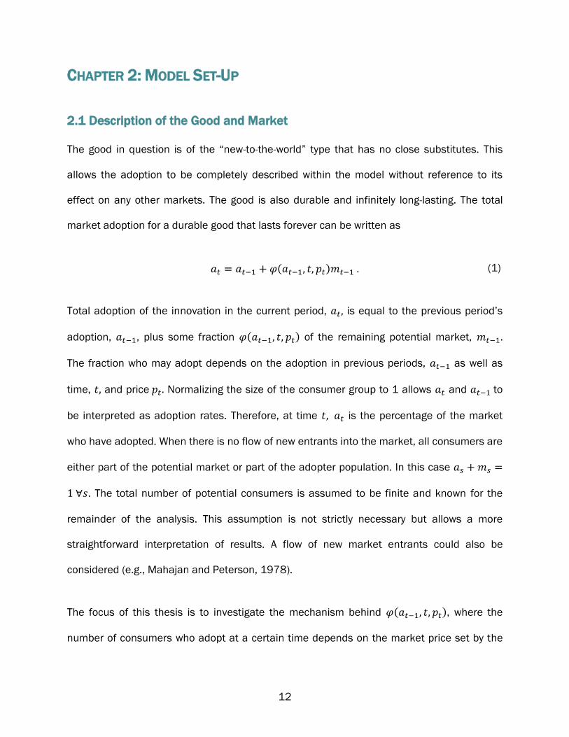
market adoption for a durable good that lasts forever can be written as

( ) (1)

Total adoption of the innovation in the current period, is equal to the previous period’s

adoption, , plus some fraction ( ) of the remaining potential market,

The fraction who may adopt depends on the adoption in previous periods, as well as

time, and price Normalizing the size of the consumer group to 1 allows and to

be interpreted as adoption rates. Therefore, at time is the percentage of the market

who have adopted. When there is no flow of new entrants into the market, all consumers are

either part of the potential market or part of the adopter population. In this case

. The total number of potential consumers is assumed to be finite and known for the

remainder of the analysis. This assumption is not strictly necessary but allows a more

straightforward interpretation of results. A flow of new market entrants could also be

considered (e.g., Mahajan and Peterson, 1978).

The focus of this thesis is to investigate the mechanism behind ( ), where the

number of consumers who adopt at a certain time depends on the market price set by the

13

firm, the size of the adopter population, and time itself. The direct time dependence of

( ) is due to a possible heterogeneity in consumer preferences. A certain

consumer may be more likely to adopt than another, and this consumer will tend to adopt in

earlier periods rather than later periods. For this reason, the fraction adopting in any time

period is time-dependent.

2.2 Consumers’ Decisions

Individual decisions have seldom been a focus in the formulation of market-wide demand in

contagion-based diffusion models. Most postulate an overall market-wide evolution of

demand (Dolan and Jeuland, 1981 and 1985; Robinson and Lakhani, 1975; Teng et al.,

1984; Thomson and Teng, 1984; and others) without reference to individual decision

making. Meanwhile, the diffusion models based on social learning and social pressure are

inherently models of heterogeneous consumers’ decisions.

Even those researchers who postulate that consumers form a valuation of the product

frequently make an assumption that the valuation comes from a random variable drawn

from a distribution without considering the logic behind the decision (Hohnisch, 2008;

Farias and Van Roy, 2010). Here, however, the choice and behaviour of consumers is

captured by the microeconomic theory of utility maximization. Consumers are assumed to be

utility maximizers who may purchase one unit of the good or none in each period. The cost of

the good is low enough that all consumers could purchase the good without being restricted

by their budget constraints. Once an individual has purchased, they are considered to be out

of the potential market and do not repurchase—no consumer purchases more than one unit.

14

After a consumer has adopted, they keep the good for the entire period of analysis. Thus,

they continue to be considered an adopter throughout all subsequent periods.

The consumers’ decision whether or not to adopt rests on several other factors:

price-dependent demand: the effect of price on individuals’ demand;

heterogeneity in price sensitivity: the effect of an individual’s price sensitivity on their

demand for the innovation;

valuation: the valuation of the good in absence of price or adoption information;

adoption-associated demand: the effect of the adoption of the innovation on an

individuals’ demand (the ‘adoption mechanism’).

The demand of individuals is then aggregated to determine the total demand in the

remainder of the market.

2.2.1 Evolution of Price-Dependent Demand

Numerous ways to include price in adoption models have been suggested and the

assumptions behind them can be divided into two distinct groups. The crucial difference

between the two approaches is the extent to which the diffusion process and price are inter-

related.

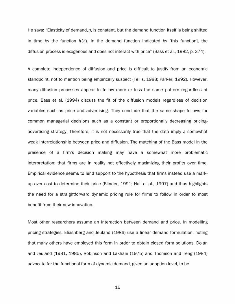
Bass (1980) proposes a model where the diffusion does not interact with price:

( ( )) ( )( ( ))

(2)

15

He says: “Elasticity of demand, , is constant, but the demand function itself is being shifted

in time by the function ( ). In the demand function indicated by [this function], the

diffusion process is exogenous and does not interact with price” (Bass et al., 1982, p. 374).

A complete independence of diffusion and price is difficult to justify from an economic

standpoint, not to mention being empirically suspect (Tellis, 1988; Parker, 1992). However,

many diffusion processes appear to follow more or less the same pattern regardless of

price. Bass et al. (1994) discuss the fit of the diffusion models regardless of decision

variables such as price and advertising. They conclude that the same shape follows for

common managerial decisions such as a constant or proportionally decreasing pricing-

advertising strategy. Therefore, it is not necessarily true that the data imply a somewhat

weak interrelationship between price and diffusion. The matching of the Bass model in the

presence of a firm’s decision making may have a somewhat more problematic

interpretation: that firms are in reality not effectively maximizing their profits over time.

Empirical evidence seems to lend support to the hypothesis that firms instead use a mark-

up over cost to determine their price (Blinder, 1991; Hall et al., 1997) and thus highlights

the need for a straightforward dynamic pricing rule for firms to follow in order to most

benefit from their new innovation.

Most other researchers assume an interaction between demand and price. In modelling

pricing strategies, Eliashberg and Jeuland (1986) use a linear demand formulation, noting

that many others have employed this form in order to obtain closed form solutions. Dolan

and Jeuland (1981, 1985), Robinson and Lakhani (1975) and Thomson and Teng (1984)

advocate for the functional form of dynamic demand, given an adoption level, to be

16

(3)

which has the feature that the demand elasticity is proportional to price:

(4)

As Bass (1980) notes, the price interacts with the diffusion process in the case of the

dynamic demand equation (4). This is important because it means that the firm has control

over the diffusion process and can spur or delay adoption by choosing different pricing

strategies.

The question of whether aggregate demand can be approximated by the above specific

functional form is empirical. Tellis (1988) notes in his meta-analysis of 367 price elasticities

in 220 markets that “it is reassuring that no significant differences in elasticity occur across

data sources, functional forms, and numbers of observations, cross-sections, and

parameters” (Tellis, 1988, p. 340), which lends credibility to the assumption of constant

price elasticity. His analysis controls for the product’s place in the adoption curve by

explicitly accounting for the evolution of demand through time as separate from the price

effect. Accumulated sales show a positive effect on the price elasticity parameter, which is

consistent with the heterogeneity assumptions herein: as a product diffuses through the

market, the less price-sensitive consumers tend to adopt in earlier periods while those with

higher price sensitivity adopt later.

From a microeconomic standpoint, one can consider the demand of each consumer as

being defined according to the probability of purchase under the assumption that

17

reservation prices are generated in a straightforward way. The whole diffusion process is

defined in probabilistic terms where, for an individual consumer who has not already

adopted, the probability of adoption in a specific time period is conditional on the total

market adoption that the consumer observes. Each consumer has only a certain probability

of forming a non-zero valuation for the product. The probability that their valuation is non-

zero is based on the diffusion mechanism, while the valuation itself is generated on the

basis of the price.

It is important to note that the commonly used functional forms are multiplicatively

separable in and . An interaction between price and the adoption rate in

previous periods is unlikely to occur as this would imply that there is a psychological

component to the absolute unit of price. Under separability, price interacts with demand in

the same way regardless of the diffusion mechanism assumed. A separable functional form

also allows us to directly analyze the effects of this aspect alone.

2.2.2 Heterogeneity of Agents

Various models have been proposed that treat consumers as completely homogeneous

(Krishnan et al., 1999), as an aggregate from multiple distinct consumer segments

(Robinson and Lakhani, 1975), and as completely heterogeneous (Kalish, 1983; Katz and

Shapiro, 1985; Chatterjee and Eliashberg, 1990; Allenby and Rossi, 1998).

There are various ways that consumers may be heterogeneous. The last two models

considered herein assume an inherent heterogeneity in the thresholds of consumers to

adopt due to social influence and information needs, respectively. However, the

heterogeneity inherent in the contagion model is fundamentally due only to exposure and is

18

not an implicit characteristic of consumers in the model. Likewise, the heterogeneity in the

purchase delay model is due only to the likelihood of making the purchase, which does not

need to be an innate trait of the individual consumer. Young (2009) shows that the

underlying shape and conclusions of the models are the same under heterogeneity for

models of this general type. Hence, adding diversity in consumers’ price sensitivity can be

straightforwardly captured by the diffusion models discussed. Here, we assume that

consumers fundamentally differ in the model-specific characteristics as well as in their

sensitivity to price. The advantage of treating the consumer group as critically individualistic

allows the approach to provide testable implications for empirical researchers. Nevo (2011)

also recommends this approach: “Interestingly, the heterogeneity in choice is only weakly

correlated with standard consumer attributes. Income, education, and family size obviously

explain some dimensions of choice, but are not enough to accurately predict consumer

behavior. Unobserved heterogeneity is important to model in many cases.”

The inclusion of a time-varying parameter controlling the probability of adoption effectively

accounts for heterogeneity in the aggregate. Each consumer in the market has an individual

probability of adoption that depends on their personal attitudes. The coefficient may also be

interpreted as a price-sensitivity parameter. Those who have lower price sensitivity therefore

have a higher probability of adoption regardless of the prevailing market price. These

consumers tend to adopt in earlier periods. Likewise, those individuals with higher sensitivity

to price have a lower probability of adoption, and these consumers tend to adopt later. In

aggregate, this shift in individual probabilities is captured by a time varying function that

describes the movement of consumers either earlier or later in the adoption progression.

19

2.2.3 Valuation of the Good

Following Jedidi and Zhang (2002), the consumer’s problem herein is set up to be

independent of other goods, which is in contrast to other methods that define a valuation in

relation to switching from an existing good (Kohli and Mahajan, 1991; Henrich, 2001;

Lamberson, 2010). The complete independence of the new good’s valuation from other

goods is more attractive in this setting because it separates the overall market for the good

in question from all other markets. In this way, there is no specific effect of adoption on any

other specific good and its price.

Each consumer establishes a valuation of the good that maximizes their individual utility,

( ), where is the new good and is a composite good that is comprised of all other

goods purchased by the consumer in the time period. The consumer has a budget constraint

. If the good is purchased, then the consumer spends on one unit of the

new good and the remainder of their budget, on purchasing the quantity

of the composite good. If the new good is not purchased, then the consumer spends

their entire budget, , on the composite, and thus can purchase

. Therefore the

consumer is indifferent between purchasing the new good and not when (

)

(

) .

The utility of the new good is determined in the following way. In each period, consumers

begin a discrete choice task of determining an acceptable price by evaluating an increasing

set of prices for the good in question. The evaluation of each individual consumer is

20

independent in every period. Adopting the good at the considered price would either provide

greater utility over non-adoption or would not. Therefore, at each price, the consumer can

either find the price acceptable or not. Individual consumers differ in their price sensitivity

and so each has a unique probability that they will find an evaluated price to be acceptable.

If the consumer finds it acceptable, the next price is evaluated in the same manner. If the

price is not acceptable, the highest acceptable price then becomes their price valuation for

that period, . Given a certain level of market adoption, a consumer will purchase if the

price is equal to or lower than their valuation of the product. Therefore, the probability that

the valuation price is at least is equal to the probability that the demand of the consumer

is 1, given full knowledge about the previous market adoption of the product.

Specifically, the valuation is such that demand is:

{

(5)

As the distance between successive prices evaluated by the consumer becomes zero, the

probability density function of valuations, given a market rate of adoption, converges to an

exponential distribution

( | ) (

| ) (6)

where is the market adoption rate—the percentage of the market who have

adopted, in periods 1 through period .

21

The market rate of evaluation, , captures the heterogeneity of price sensitivity among

consumers. The consumers evaluating the product in each period differ because those with

lower price sensitivity have a higher likelihood of purchase in earlier periods. Therefore the

parameter can be interpreted as the market-wide price sensitivity. It is time-dependent

and increasing in so that —the market becomes more price-sensitive through

time with even a small amount of heterogeneity in price sensitivity. Adopters whose price

sensitivity is low tend to adopt in earlier periods because they are more likely to find the

market price acceptable. As time progresses, the more price sensitive consumers remain in

the market. For this reason, the market-wide price sensitivity may increase through time due

solely to consumer heterogeneity.

An attractive implication of this formulation of valuations is that regardless of how many

prices the consumer has evaluated, the probability that the next valuation becomes their

reservation price is constant. This means that there is no bias in the absolute price level,

suggesting that valuations for more expensive goods, such as cars, and those that are

relatively inexpensive, such as small electronics, are not inherently different and can be

analyzed using the same model.

Another appealing feature is that the memorylessness of the valuation choices assumed

implies that a consumer could begin to evaluate prices at any level with no alteration of their

likely valuation. Price-choice methodologies that are presently used in empirical applications

where the researcher chooses a minimal feasible evaluation price, such as in discrete

choice analysis, monadic testing, or a variant of the price sensitivity meter, could thus be

directly used to gauge valuations.

22

Jedidi and Zhang’s (2002) empirical testing for their conjoint approach to measuring

reservation prices seems to suggest an approximately exponential aggregate demand in the

higher price levels but with an unanticipated interaction at the low-end of feasible

reservation prices. An interaction with quality and price has been empirically examined and

shown to have a curious effect (Ding et al., 2010) resulting in an inverted n-shaped demand

curve. The van Westendorp price sensitivity meter (van Westendorp, 1976), a frequently

used method in empirical pricing research that has been recently advanced to better match

firm optimization (Roll et al., 2010), also assumes a psychological effect of low prices. These

empirical results suggest that additional care should be taken when using introductory

pricing offers so as not to negatively affect quality perceptions.

Price-quality implications are an important area of research and provide a counterpoint to

some of the conclusions in the present framework. Bagwell and Riordan (1991) show the

significance of quality’s repercussions on price in a dynamic environment and find a

monotonically decreasing price due to the loss of the potency of the quality signal through

time. However, their model does not account for a positive effect of adoption on aggregate

demand, which is the principal reason for the disagreement between our conclusions.

2.2.4 Adoption-associated demand

The second component in the consumer’s valuation of the product is the macroscopic

information about adoption in the market. A direct effect of the adoption level on valuation

has been investigated in other literature, a phenomena often termed “network effects.” In

this literature, the size of the network itself impacts adoption. This is relevant for products

where a large network size adds to the value of the products. Katz and Shapiro (1994) give

23

the example of “a communications network, such as the public telephone system, where

various end users join a system that allows them to exchange messages with one another.

Joining such a network is valuable precisely because many other households and

businesses obtain components of the overall system … Because the value of membership to

one user is positively affected when another user joins and enlarges the network, such

markets are said to exhibit ‘network effects,’ or ‘network externalities’” (Katz and Shapiro,

1994, p.94). Network effects are important components for a special class of products, but

these effects are small in general for new products. Specifically, for the products considered

herein, we assume that there is no incremental value when the network of current users is

large compared to when the adopter population is small.

Here, the adoption affects consumers’ valuations through the adoption mechanism rather

than directly. Consumers’ final valuations are based on the market adoption they have

observed throughout its life cycle. The valuation is described in probabilistic terms, which

means that each individual has a certain likelihood of forming a valuation in each period.

This probability is based on the adoption in previous periods and is characteristic of the

adoption mechanism. Therefore,

( | )

( ) (7)

The probability of adoption given a price is a function of adoption in the previous periods.

This measure is established by the underlying diffusion process and differs for each of the

four product classes considered. The explicit formulation of this element is discussed in

relation to the specific mechanisms.

24

2.2.5 Aggregation of Demand

In each period, ( ) consumers are left in the market and may purchase.

Consumers observe the market adoption to calculate their valuations. The size of the group

of consumers is normalized to 1 so that demand can be interpreted as a rate: the

percentage of the market who adopt in each period. All consumers who have formed a price-

valuation have a valuation of at least zero, which means that the cumulative distribution

function (CDF) of the price-valuations is given by

( ) ( ) (8)

The fraction of consumers who have made such a valuation is a proportion of the total

remaining market, , given by

( ) ( ) (9)

where ( ) is the aggregation of individual probabilities dependent on market

adoption. Therefore the aggregate demand in the period is

( ) ( ) (10)

Aggregate demand is separable in ( ) and . The foregoing is a complete

description of the demand side.

2.3 Behaviour of Firms

As Robinson and Lakhani (1975) note, much price theory has been focused on static

settings, making the results less useful for managers acting in dynamic markets. Initially,

25

focus in the literature was on comparing various “rule of thumb” pricing strategies, such as

a constant mark-up or a completely static price, to marginal pricing strategies. They observe

that: “A manager who has some insight into how his costs and markets are going to evolve

… can incorporate his ideas into a dynamic pricing model which, for a rapidly evolving

business, can greatly enhance his long run performance” (Robinson and Lakhani, 1975, p.

1114).

Firms are assumed to seek to maximize their profit. In contrast to static decision-making,

they maximize their total profit throughout the planning period. Robinson and Lakhani

(1975) note that, “since most corporations are in business for the long run, a major

parameter in any price model should be the integrated profit obtained throughout some

appropriate planning period” (Robinson and Lakhani, 1975, p. 1114).

Many diffusion models explicitly consider the effect of discounting future profits (Kalish,

1985, for example). However, the period under consideration herein occurs prior to

competitive entry, where the firm maintains a monopoly position. This time period is

assumed to be short and for this reason, discounting during the planning period is not

considered to be an important consideration in the model.

In the single-firm, single-good environment, maximization of profit is an obvious choice for a

firm’s strategy. This is inherently an abstraction from real-world strategies: many firms

introduce new products for other reasons, such as to benefit from line extension or to

complement existing products, as a strategy to be considered as an acquisition target, or as

an initiative to increase brand equity. For this reason, maximization of the profit from the

single new product may be too simplistic to capture the true motivations for firms to

26

introduce innovative products into the marketplace. The aforementioned areas are

important extensions to the present models.

Firms are also assumed to be able to accurately measure and predict the market demand

for their product among those who are willing to adopt. Many traditional and new ways to

estimate and measure these specifics are widely used by industry and academic

researchers alike (Bergstein and Estelami, 2002 provides an overview of traditional and new

empirical techniques in pricing research). The assumption that firms have this knowledge to

inform their planning is therefore not a significant departure from data that real-world firms

are able to obtain.

We also assume that the firm is perfectly flexible in meeting whatever demand arises and

meets this demand each period. The firm does not hold inventory, nor does it incur different

costs for a higher or lower production level. This is a more problematic assumption,

especially in the case of a very small firm introducing a truly innovative product. In the case

where an established firm introduces a blockbuster new product, the assumption is less

limiting. The firm’s decision taking into account intertemporal firm-level considerations, such

as a motivation for production or profit stability, would be interesting to investigate, but is

beyond the scope of this thesis.

Under the assumptions that the firm’s objective is to maximize profit, that their

measurements of demand are accurate, and that they are able to produce to meet any

demand they face, the multi-period optimization problem then turns into one akin to a static

economies-of-scope problem. The monopoly firm is able to fully internalize its own effect on

future demand and thereby optimize over the entire time period. In this way, the firm is able

27

to create a pricing strategy through time that yields the most benefit to it taking into account

the characteristics of adopters.

2.3.1 Costs of Production

One of the advantages to a firm of being first to market is that it gains valuable production

experience before competitors enter. Robinson and Lakhani (1975) were among the first to

incorporate the firm’s costs and decision variables into a diffusion model.

There are two general ways to conceptualize firm learning of this type. One is for the

efficiencies of the firm to depend on the amount produced, regardless of time. This would

mean that, regardless of how long it took the firm to produce the first few units, the

efficiencies gained are the same. This is the approach taken by many researchers (Robinson

and Lakhani, 1975; Bass, 1982). Common approaches assume that the average cost to the

firm takes the form

( )

(11)

The range for the parameter is taken by Robinson and Lakhani (1975) to be .

Bass (1982) suggests that the preceding equation describes instead the marginal cost.

Another way that firms’ costs could evolve (Eliasberg and Jeuland,1986) is to allow the costs

to vary with time, independent of the level of production. In the case of constant marginal

costs, the (total) cost function takes the form

( ) (12)

28

where is the marginal cost at time t, which is usually taken to be non-increasing in t. A

time-varying, per-unit cost provides a more convenient maximization framework in the

discrete case, as the problem maximizing profit reduces to the problem of maximizing the

net margin in each period.

The major difference between a cost function that varies with time and a cost function that

varies with production level will appear when the firm’s production level varies considerably

across time. When the amount produced each period is similar, the two approaches will

yield similar results.

The development costs of new products may also take the form of so-called “non-recurring

engineering costs” for many types of innovative products. For example, software products,

most media, and many industrial design inventions are characterized by a large cost for their

creation and almost no cost for their distribution. The cost function for the firm in these

cases is essentially a one-time fixed cost which does not depend on the eventual production

level. This cost then does not affect the firm’s pricing decision through time.

In general, costs obviously have an effect on the firm’s decision; however, the effect of a

constant or increasing period-dependent cost on the optimum is analytically the same as

considering a single fixed cost and interpreting the optimal prices as margins rather than

absolute prices. The problem of costs therefore is of less interest than the effect of the

diffusion mechanism itself on the optimal strategy through time. For this reason, they are

not central to the analysis below.

29

2.3.2 Feasibility of Results

Models associated with the diffusion literature, especially with regards to diffusion by

contagion, have mostly endeavoured to maximize the discounted flow of profits by having a

continuously varying price and cost. While mathematically attractive, this approach is less

appealing from a practical standpoint. Firms simply can’t and don’t continuously vary their

price. A major aim of the present thesis is to explore a set of more realistic pricing strategies

where the firm anticipates and measures adoption at various intervals. This allows a way for

the model’s predictions to be empirically tested and the strategies recommended to be

executed by firms.

Another drawback of fully dynamic solutions is the continuous flow of sales and costs that

are known and reacted to immediately by the firm. Measuring the market adoption is

especially difficult for competitive firms as competitors are rarely forthcoming with their

sales numbers. Thus, as soon as there is competitive entry, the firm loses its ability to

accurately measure the total market sales along with its own market share. These present

very significant practical drawbacks in relation to the use of continuous-time models.

Fortunately, total market adoption can be estimated at interval and reacted to in due

course. For this reason, a discrete-time framework is the most appropriate and is therefore

the one that we have chosen to use.

2.3.3 Competition

The period under study in the current model is the phase before competitive entry in the

market. The assumption that no competitors enter for the duration of the planning period

allows the firm complete control over the pricing of the product in all periods. For many

30

firms, the period of lack of competition is the motivation for introducing new products. As

Metcalfe (1998) notes: “competition behaviour is in part motivated by the search for

monopoly positions” (Metcalfe, 1998, p. 18).

A competitor entering partway through the planning period has an effect on both the price

pattern and adoption within the market. If the incumbent firm correctly anticipates

competitive entry, their planning will be affected. The potential profit made by the firm is

largest prior to competitive entry when they maintain a monopoly position. In this portion of

the planning period, the firm can employ the most aggressive strategies to maximize

intertemporal profit as they will be the sole beneficiary of the increased demand in later

periods. Once there is competitive entry, the profits made by the firm decrease toward zero

as the number of firms entering increases. As more competitors enter, the firm is not able to

benefit as much by pursuing aggressive pricing strategies at the beginning of the planning

period. The analytical limit is the case of perfect competition. In this case, the firm cannot

benefit at all from an increased demand in later periods because it makes no profit. The

firm, therefore, can only profit in periods before competitive entry occurs. In this case, the

optimal pricing strategy for the firm becomes identical to that of a firm that plans only if it

anticipates that competitors will enter the market.

Industry dynamics and interactions due to competition have been incorporated into various

diffusion models (Eliashberg and Chatterjee, 1985; Katz and Shapiro, 1985; Rao and Bass,

1985; Jovanivic and MacDonald, 1994; Bergemann and Valimaki, 1997; Vettas, 1998;

among others). However, the interesting effects come from the nature of the competition

examined. Differences in vertical or horizontal product differentiation, such as diversity in

31

quality or characteristics and differences in firms’ considerations, such as costs, production

capacity, product line, brand image, and reputation, are important extensions to the present

model.

2.4 Market Size, Full Adoption, and Underadoption

A crucial nuance in the adoption literature is the divergence between various disciplines

regarding the idea of “full adoption,” the case where all potential consumers adopt as the

number of time periods approaches infinity. In the marketing literature, where diffusion is

based on contagion and the population is fully mixed, full adoption is inevitable. However,

the inevitability of full adoption hinges on the structureless nature of interactions. Here,

each individual is equally likely to interact with every other. When a social network structure

is added, for example, “underadoption traps” (Choi et al., 2010) are possible. Empirical

research would suggest that many new products never reach full saturation.

In some of the models described herein, there are situations in which full adoption is

impossible but which differ from the underadoption traps discussed above. In these models

the inability to achieve full adoption is due to the characteristics of the adopter population

itself and not to the market’s structure: an individual who will never adopt when they are in a

certain population may have adopted if they were in a different population. This suggests

that they should still be considered potential adopters, much like those who do not adopt

when the structured market falls into an underadoption trap.

32

CHAPTER 3: DELAYED PURCHASE

3.1 Diffusion Due to Delayed Purchase

As discussed in Chapter 1, innovations do not diffuse all at once, but rather are adopted

gradually. Simply separating the decision to purchase a product from the actual purchase

transaction itself can result in time-dependent adoption of the new product.

The product that the firm wishes to introduce in this model is deliberately simplistic in order

to allow a comparison with the subsequent models: consumers all already wish to adopt the

product and will do so at the earliest opportunity, provided that the price of the product is

acceptable. Consumers, however, vary in their opportunity for purchase. For example, it may

be that the consumer goes to the store only every so often. In this case, future adoption

does not depend on the current adoption rate but, instead, each consumer has an individual

probability of adoption in each time period.

The elasticity of demand and the size of the market are known by the firm and so the firm’s

effects on these factors can be internalized. Because all consumers are willing purchasers

given a certain valuation, the firm can use an intertemporal pricing strategy in order to

maximize its profit over the whole time period.

3.2 Model Framework

Consumers at the beginning of the planning period all have an individual probability of

having an opportunity to purchase the good, , and forming a product valuation. This can

be interpreted as the individual’s probability of going to the store where the product is sold.

Suppose that is the aggregate of the individual consumers’ probabilities, which can be

33

interpreted as the fraction of consumers who may purchase in time period . The parameter

may time-vary since consumers may be more or less likely to have an opportunity to

purchase. Therefore, those who are more likely to do so tend to adopt earlier. The aggregate

demand at a certain price level is simply given as a time-dependent fraction and does not

depend on the market adoption. Consequently,

( ) (13)

The parameter does not depend on Therefore, the price-independent

adoption in period is

( ) ( ) (14)

At time , the total market adoption, , is the total adoption in the last period, , plus

some fraction, , of those who are left to adopt, . Equation (14) describes the

maximum adoption if the good were available at no cost. Note that even if the good was

free, adoption would be gradual, which is consistent with one of the basic empirical results

of new product adoption.

Incorporating the consumers’ price sensitivity gives the following market demand in each

period:

( ) ( ) ( ) (15)

which means that inverse demand is given by solving (15) for so that

34

(

( ∑ )

) (16)

This means that the firm’s -period profit maximization problem is

{∑

(

( ∑ )

)

} (17)

The effect of the fraction is a scaling factor on optimal production that does not affect the

optimal pricing policy. The firm optimizes as if regardless of its value. Therefore, it is

omitted from the remainder of the analysis in favour of analyzing

3.3 Optimization Results

3.3.1 Summary of Key Results

The maximization problem faced by the firm in Subsection 3.2 can be numerically solved for

any given length of planning horizon. Figure 1 shows an example of the solution to the firm’s

optimization problem over eight periods, assuming a constant value of and

Numeric and theoretical solutions are found in appendix section A3.2.

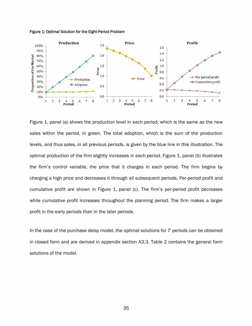
35

Figure 1: Optimal Solution for the Eight-Period Problem

Figure 1, panel (a) shows the production level in each period, which is the same as the new

sales within the period, in green. The total adoption, which is the sum of the production

levels, and thus sales, in all previous periods, is given by the blue line in this illustration. The

optimal production of the firm slightly increases in each period. Figure 1, panel (b) illustrates

the firm’s control variable, the price that it charges in each period. The firm begins by

charging a high price and decreases it through all subsequent periods. Per-period profit and

cumulative profit are shown in Figure 1, panel (c). The firm’s per-period profit decreases

while cumulative profit increases throughout the planning period. The firm makes a larger

profit in the early periods than in the later periods.

In the case of the purchase delay model, the optimal solutions for periods can be obtained

in closed form and are derived in appendix section A3.3. Table 2 contains the general form

solutions of the model.

36

Table 2: Optimal Solutions for the Purchase Delay Model

General Form of the Optimal Solutions

Production ( ∑

) ( ∑

( ∑ )

)

Price ∑

( ∑ )

Profit ∑( ∑

( ∑ )

)( ∑

) ( ∑

( ∑ )

)

Adoption ∑( ∑

) ( ∑

( ∑ )

)

3.3.2 Pricing Strategy

The pricing strategy is straightforward for the firm where adoption is delayed only by the

consumer’s likelihood of being in a purchase situation. The difference in successive periods’

prices is given as

∑

(18)

The result in equation ((18) is derived in section A3.3.2. The value of

∑

is always

positive since ∑ and . Therefore,

. This means that firm always employs a price skimming strategy for the entire period.

Figure 2 illustrates the firm’s optimal pricing strategy for the eight-period case. In line with

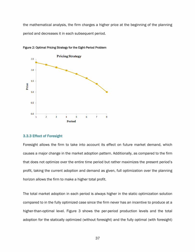
37

the mathematical analysis, the firm charges a higher price at the beginning of the planning

period and decreases it in each subsequent period.

Figure 2: Optimal Pricing Strategy for the Eight-Period Problem

3.3.3 Effect of Foresight

Foresight allows the firm to take into account its effect on future market demand, which

causes a major change in the market adoption pattern. Additionally, as compared to the firm

that does not optimize over the entire time period but rather maximizes the present period’s

profit, taking the current adoption and demand as given, full optimization over the planning

horizon allows the firm to make a higher total profit.

The total market adoption in each period is always higher in the static optimization solution

compared to in the fully optimized case since the firm never has an incentive to produce at a

higher-than-optimal level. Figure 3 shows the per-period production levels and the total

adoption for the statically optimized (without foresight) and the fully optimal (with foresight)

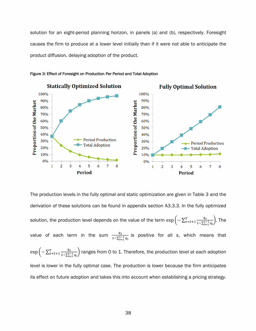
38

solution for an eight-period planning horizon, in panels (a) and (b), respectively. Foresight

causes the firm to produce at a lower level initially than if it were not able to anticipate the

product diffusion, delaying adoption of the product.

Figure 3: Effect of Foresight on Production Per Period and Total Adoption

The production levels in the fully optimal and static optimization are given in Table 3 and the

derivation of these solutions can be found in appendix section A3.3.3. In the fully optimized

solution, the production level depends on the value of the term ( ∑

∑

). The

value of each term in the sum

∑

is positive for all s, which means that

( ∑

∑

) ranges from 0 to 1. Therefore, the production level at each adoption

level is lower in the fully optimal case. The production is lower because the firm anticipates

its effect on future adoption and takes this into account when establishing a pricing strategy.

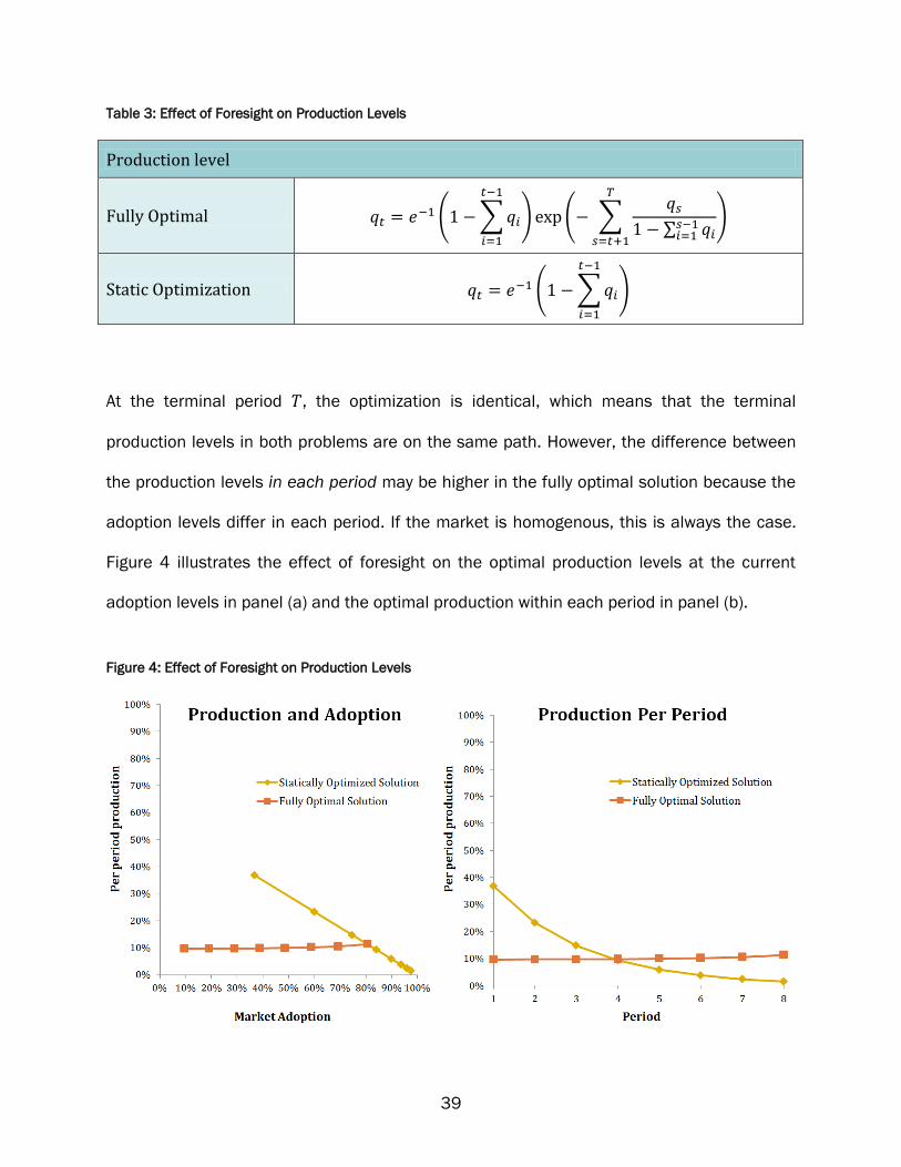
39

Table 3: Effect of Foresight on Production Levels

Production level

Fully Optimal ( ∑

) ( ∑

∑

)

Static Optimization ( ∑

)

At the terminal period , the optimization is identical, which means that the terminal

production levels in both problems are on the same path. However, the difference between

the production levels in each period may be higher in the fully optimal solution because the

adoption levels differ in each period. If the market is homogenous, this is always the case.

Figure 4 illustrates the effect of foresight on the optimal production levels at the current

adoption levels in panel (a) and the optimal production within each period in panel (b).

Figure 4: Effect of Foresight on Production Levels

40

As found in the mathematical results, the optimal production of the firm at each level of

adoption is lower in the fully optimal solution; the firm overproduces as compared with the

optimum when it does not anticipate its own effect on future demand. This effect is shown in

Figure 4, panel (a). However, as Figure 4, panel (b) illustrates, comparing the results period

by period shows no consistent pattern. The lack of a pattern is due to the dependence of the

optimum on the adoption level, as illustrated in panel (a), rather than on the period,

illustrated in panel (b).

The effect of foresight on the price path is also straightforward. The general form solutions

for the period price for both optimization procedures are given in Table 4 and are derived

in appendix sections A3.3.1 and A3.3.3.

Table 4: Effect of Foresight on Optimal Price

Price

Fully Optimal ∑

∑

Static Optimization

The price in the fully optimized solution is higher than in the static optimization for all

periods, with the exception of the last period, when they are equal. Figure 5 illustrates the

effect of foresight on the optimal pricing strategy. As derived in the mathematical results,

the optimal price is higher than the price charged by the statically optimizing firm.

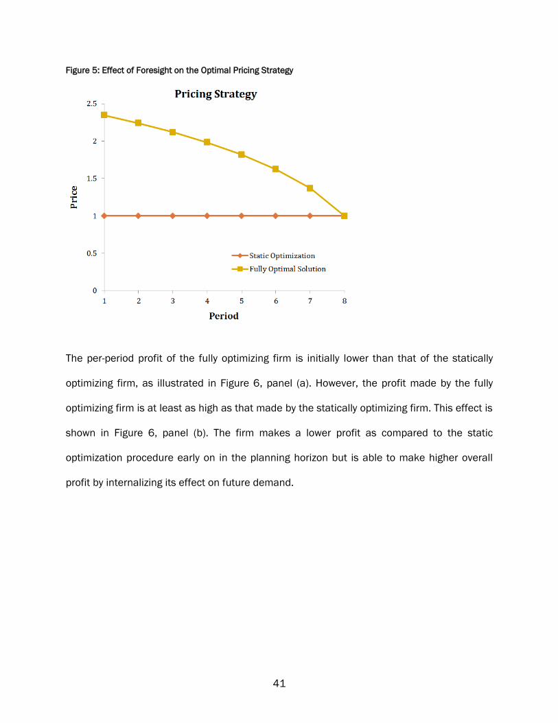
41

Figure 5: Effect of Foresight on the Optimal Pricing Strategy

The per-period profit of the fully optimizing firm is initially lower than that of the statically

optimizing firm, as illustrated in Figure 6, panel (a). However, the profit made by the fully

optimizing firm is at least as high as that made by the statically optimizing firm. This effect is

shown in Figure 6, panel (b). The firm makes a lower profit as compared to the static

optimization procedure early on in the planning horizon but is able to make higher overall

profit by internalizing its effect on future demand.

42

Figure 6: Effect of Foresight on Profit

3.3.4 Effect of Heterogeneity

Adding heterogeneity of price sensitivity does not change the nature of the pricing strategy

itself. Even as heterogeneity increases, the optimal pricing policy is for prices to decrease

through time for the entire planning horizon. The difference in period-over-period prices with

heterogeneity is

(

∑

) (19)

The general form of the pricing strategy shown in equation (19) is derived in appendix

section A3.3.1.2. The term

∑

is strictly positive and, since the difference

between successive prices is always strictly negative: . As increases, the

price difference also increases, which causes the path of prices to become steeper through

time. These mathematical results can be seen by comparing the low and high heterogeneity

solutions in Figure 7, panels (a) and (b).

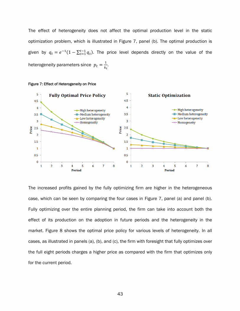
43

The effect of heterogeneity does not affect the optimal production level in the static

optimization problem, which is illustrated in Figure 7, panel (b). The optimal production is

given by ( ∑ ) The price level depends directly on the value of the

heterogeneity parameters since

.

Figure 7: Effect of Heterogeneity on Price

The increased profits gained by the fully optimizing firm are higher in the heterogeneous

case, which can be seen by comparing the four cases in Figure 7, panel (a) and panel (b).

Fully optimizing over the entire planning period, the firm can take into account both the

effect of its production on the adoption in future periods and the heterogeneity in the

market. Figure 8 shows the optimal price policy for various levels of heterogeneity. In all

cases, as illustrated in panels (a), (b), and (c), the firm with foresight that fully optimizes over

the full eight periods charges a higher price as compared with the firm that optimizes only

for the current period.

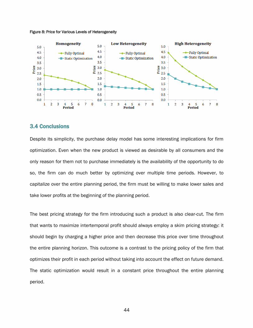
44

Figure 8: Price for Various Levels of Heterogeneity

3.4 Conclusions

Despite its simplicity, the purchase delay model has some interesting implications for firm

optimization. Even when the new product is viewed as desirable by all consumers and the

only reason for them not to purchase immediately is the availability of the opportunity to do

so, the firm can do much better by optimizing over multiple time periods. However, to

capitalize over the entire planning period, the firm must be willing to make lower sales and

take lower profits at the beginning of the planning period.

The best pricing strategy for the firm introducing such a product is also clear-cut. The firm

that wants to maximize intertemporal profit should always employ a skim pricing strategy: it

should begin by charging a higher price and then decrease this price over time throughout

the entire planning horizon. This outcome is a contrast to the pricing policy of the firm that

optimizes their profit in each period without taking into account the effect on future demand.

The static optimization would result in a constant price throughout the entire planning

period.

45

Greater heterogeneity in the adopter population also causes a significant effect on the firm’s

optimal strategy. When there is a high degree of heterogeneity among consumers, the

steepness of the period-over-period prices increases. The optimal pricing strategy shifts

because the firm is able to take into account the lower price-sensitivity of consumers who

adopt in earlier periods.

46

CHAPTER 4: DIFFUSION BY AWARENESS

4.1 Awareness as a Diffusion Mechanism

A firm may wish to take a product to market that is easily understood by consumers when

they become aware of it for the first time. For instance, a product that is a clearly

communicated line expansion, such as a new album by an established artist or a new novel

by a well-known author, is simple to convey to consumers and needs little additional

explanation. The diffusion of an exclusive product sold by a recognisable store that has

moved into a new market would also need little additional explanation. Because of prior

mass-market advertising efforts, many consumers would already have an understanding of

the product. Consumers would need no additional information to decide whether or not to

adopt besides the product’s availability.

In the field of marketing, the product diffusion model of Bass (1969) has been widely used

to understand and explain the adoption of a new product of this type. Bass’s model is based

on a very simple principle: new products diffuse through a market in much the same way as

a disease spreads through a population. At each point in time, an individual in the market

has a certain likelihood of adopting based on the previous adoptions of other market agents.

In this way, adoption relies on a channel of information that flows among market

participants. Extensions due to Kalish (1983, 1985) adding firm optimization of pricing and

Krishnan, Bass, and Jain (1999) adding demand sensitivity to price allow diffusion models of

this type to be explored from an economic standpoint.

47

An interpretation of this model can be explained by analogy. The problem is similar to that

faced by an ice cream vendor in a park with many people milling around on a hot summer

day. At the beginning, there are a few people who really want ice cream and actively seek

out an ice cream stand. Most people are walking about and enjoying their day. They may

spontaneously consider getting ice cream but, more likely, they will think about it only if they

see someone else walking by with an ice cream cone. As more ice cream cones are sold, the

likelihood of someone without a cone running into someone enjoying one is very high, and

thus the likelihood of each person thinking of getting ice cream also increases. For the ice

cream vendor, it may be optimal to sell at a very low price, or even give away a few free

cones and send those customers through the crowd to show others that ice cream is

available.

Our firm’s decision is fundamentally the same. Formally, the diffusion mechanism is

described in the following way. Each member of the potential market has a certain

probability of adoption that is independent of the current market adoption level and a

probability of adoption that is proportional to the size of the current adopter population. The

two forces have been described as the coefficient of innovation and the coefficient of

imitation, and as indicating an external and internal influence, respectively (Bass, 1969;

Lekvall and Wahlbin, 1973; Bass et al., 1980). They are often interpreted as the effect of

the advertising channel and the effect of the word-of-mouth channel.

Because the only two effects on the consumer’s purchase are advertising and word-of-

mouth, any product that may need additional explanation to persuade consumers that a

purchase would be desirable would not be appropriate to the framework considered here.

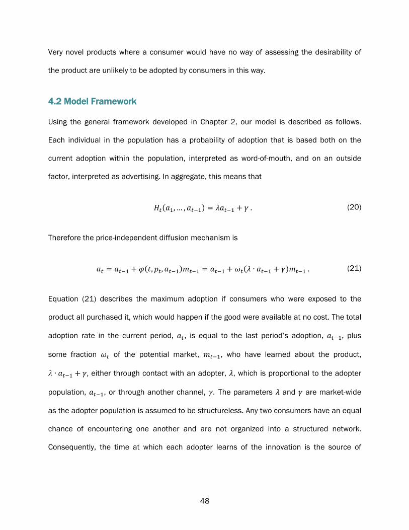
48

Very novel products where a consumer would have no way of assessing the desirability of

the product are unlikely to be adopted by consumers in this way.

4.2 Model Framework

Using the general framework developed in Chapter 2, our model is described as follows.

Each individual in the population has a probability of adoption that is based both on the

current adoption within the population, interpreted as word-of-mouth, and on an outside

factor, interpreted as advertising. In aggregate, this means that

( ) (20)

Therefore the price-independent diffusion mechanism is

( ) ( ) (21)

Equation (21) describes the maximum adoption if consumers who were exposed to the

product all purchased it, which would happen if the good were available at no cost. The total

adoption rate in the current period, , is equal to the last period’s adoption, , plus

some fraction of the potential market, , who have learned about the product,

either through contact with an adopter, , which is proportional to the adopter

population, , or through another channel, The parameters and are market-wide

as the adopter population is assumed to be structureless. Any two consumers have an equal

chance of encountering one another and are not organized into a structured network.

Consequently, the time at which each adopter learns of the innovation is the source of

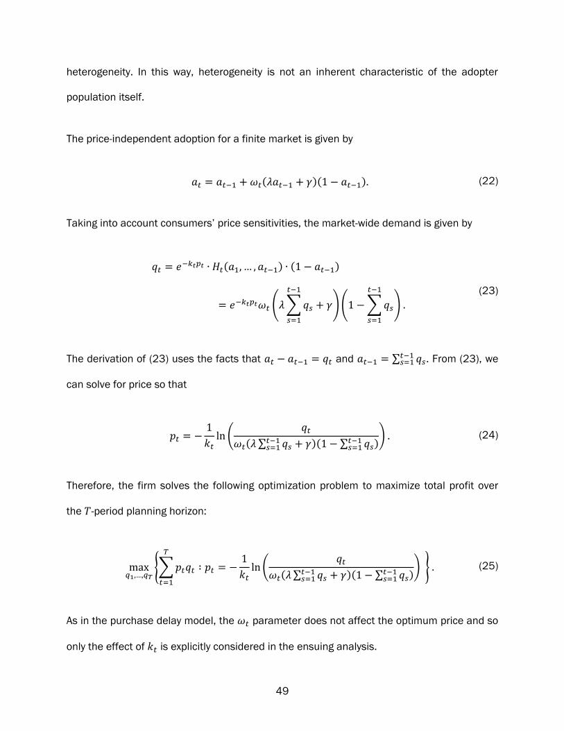
49

heterogeneity. In this way, heterogeneity is not an inherent characteristic of the adopter

population itself.

The price-independent adoption for a finite market is given by

( )( ) (22)

Taking into account consumers’ price sensitivities, the market-wide demand is given by

( ) ( )

( ∑

)( ∑

)

(23)

The derivation of (23) uses the facts that and ∑ . From (23), we

can solve for price so that

(

( ∑ )( ∑

)

) (24)

Therefore, the firm solves the following optimization problem to maximize total profit over

the -period planning horizon:

{∑

(

( ∑ )( ∑

)

)

} (25)

As in the purchase delay model, the parameter does not affect the optimum price and so

only the effect of is explicitly considered in the ensuing analysis.

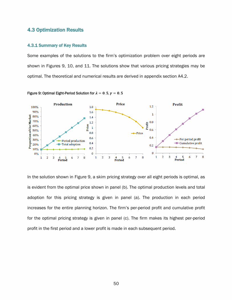
50



Some examples of the solutions to the firm’s optimization problem over eight periods are

shown in Figures 9, 10, and 11. The solutions show that various pricing strategies may be

optimal. The theoretical and numerical results are derived in appendix section A4.2.

Figure 9: Optimal Eight-Period Solution for

In the solution shown in Figure 9, a skim pricing strategy over all eight periods is optimal, as

is evident from the optimal price shown in panel (b). The optimal production levels and total

adoption for this pricing strategy is given in panel (a). The production in each period

increases for the entire planning horizon. The firm’s per-period profit and cumulative profit

for the optimal pricing strategy is given in panel (c). The firm makes its highest per-period

profit in the first period and a lower profit is made in each subsequent period.

51


Figure 10 illustrates a case where the firm’s optimal strategy over eight periods gives rise to

a penetration pricing strategy in the early periods and a skim pricing strategy in the later

periods. Panel (a) of Figure 10 shows that the production levels at the optimal price set by

the firm increases throughout the entire planning period. Figure 10, panel (b) illustrates the

specific price levels of the solution: the price continues to increase until period 6, after

which the firm decreases the price for the remainder of the planning period. Per-period profit

and cumulative profit are shown in panel (c). The firm’s per-period profit increases for the

first part of the planning period but begins to decrease towards the end while cumulative

profit increases throughout.

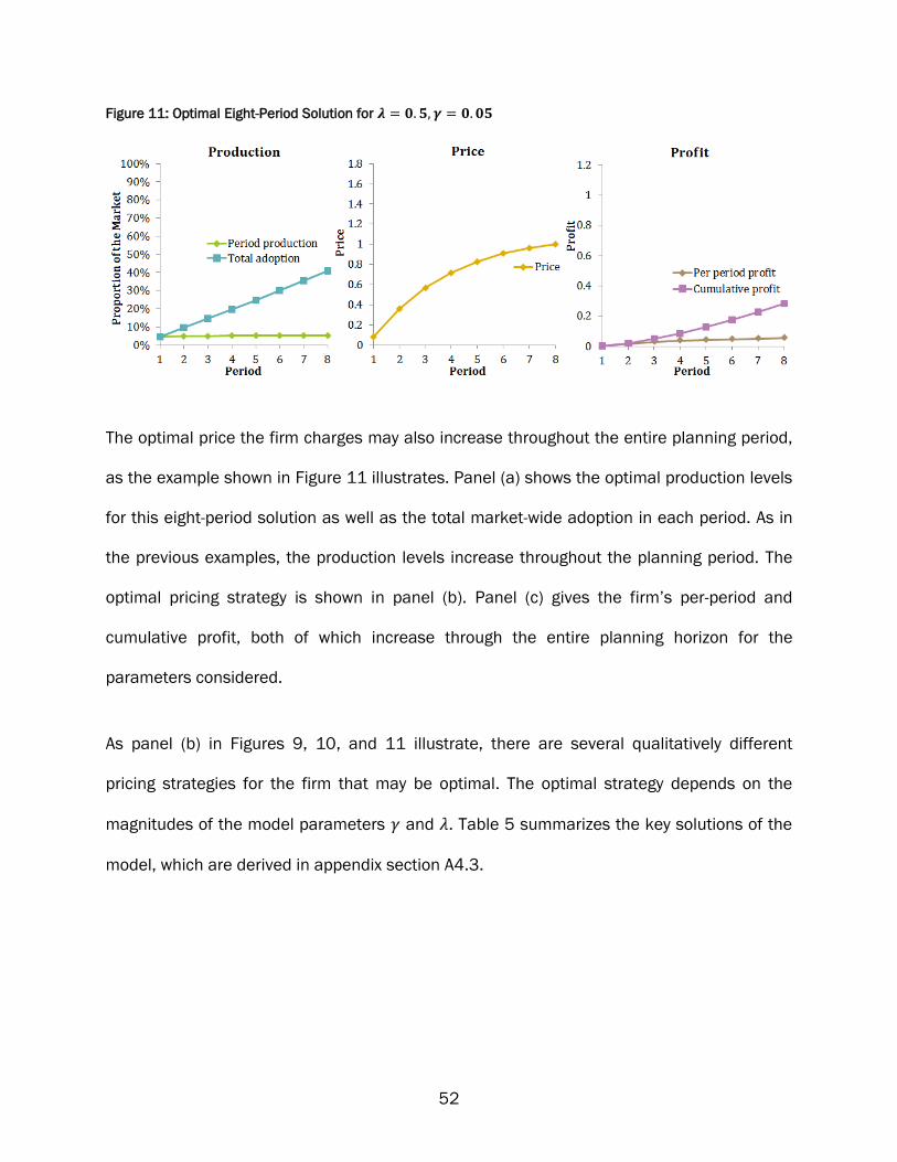
52


The optimal price the firm charges may also increase throughout the entire planning period,

as the example shown in Figure 11 illustrates. Panel (a) shows the optimal production levels

for this eight-period solution as well as the total market-wide adoption in each period. As in

the previous examples, the production levels increase throughout the planning period. The

optimal pricing strategy is shown in panel (b). Panel (c) gives the firm’s per-period and

cumulative profit, both of which increase through the entire planning horizon for the

parameters considered.

As panel (b) in Figures 9, 10, and 11 illustrate, there are several qualitatively different

pricing strategies for the firm that may be optimal. The optimal strategy depends on the

magnitudes of the model parameters and . Table 5 summarizes the key solutions of the

model, which are derived in appendix section A4.3.

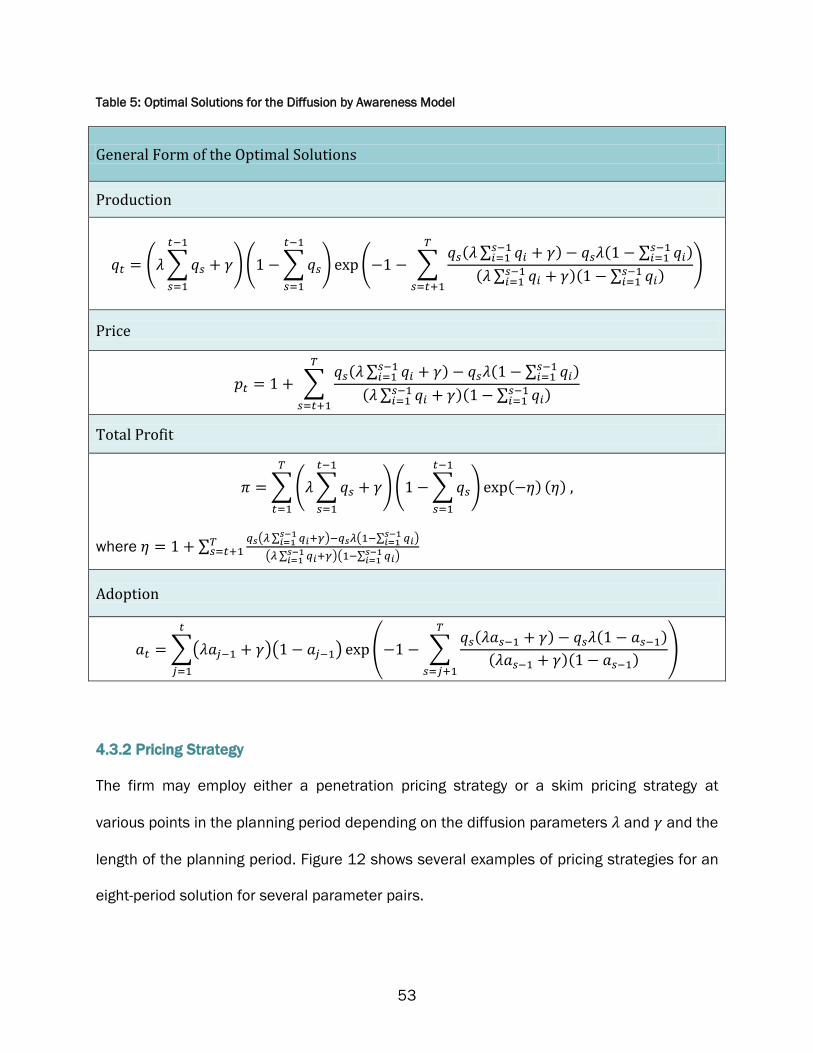
53

Table 5: Optimal Solutions for the Diffusion by Awareness Model


Production

( ∑

)( ∑

) ( ∑ ( ∑

) ( ∑

)

( ∑ )( ∑

)

)

Price

∑ ( ∑

) ( ∑

)

( ∑ )( ∑

)

Total Profit

∑( ∑

)( ∑

) ( ) ( )

where ∑ ( ∑

) ( ∑

)

( ∑ )( ∑

)

Adoption

∑( )( ) ( ∑ ( ) ( )

( )( )

)


The firm may employ either a penetration pricing strategy or a skim pricing strategy at

various points in the planning period depending on the diffusion parameters and and the

length of the planning period. Figure 12 shows several examples of pricing strategies for an

eight-period solution for several parameter pairs.

54

Figure 12: Pricing Strategy for Various Parameter Pairs

The price difference between subsequent periods is given as

( )

( )( ) (26)

The period-over-period pricing strategy shown in equation (26) is derived in appendix section

A4.3.2. A skim pricing strategy is always optimal when over one half of the market has

adopted. The sign of equation (26) depends on the sign of since

( )( )

If the adoption rate, , is above 50 percent, then this expression is negative because

Therefore the optimal period-over-period price is always decreasing through time.

Initially, when the adoption in the market, , is low, the pricing strategy depends mostly on

the relative size of the and and is only mildly affected by the market size effect,

Here, either one of the two strategies may be best. The dependence on the imitation and

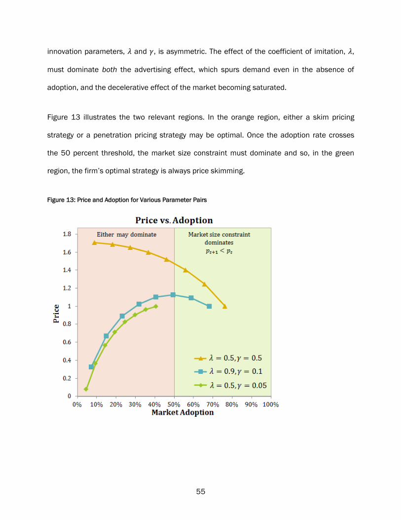
55

innovation parameters, and , is asymmetric. The effect of the coefficient of imitation, ,

must dominate both the advertising effect, which spurs demand even in the absence of

adoption, and the decelerative effect of the market becoming saturated.

Figure 13 illustrates the two relevant regions. In the orange region, either a skim pricing

strategy or a penetration pricing strategy may be optimal. Once the adoption rate crosses

the 50 percent threshold, the market size constraint must dominate and so, in the green

region, the firm’s optimal strategy is always price skimming.

Figure 13: Price and Adoption for Various Parameter Pairs

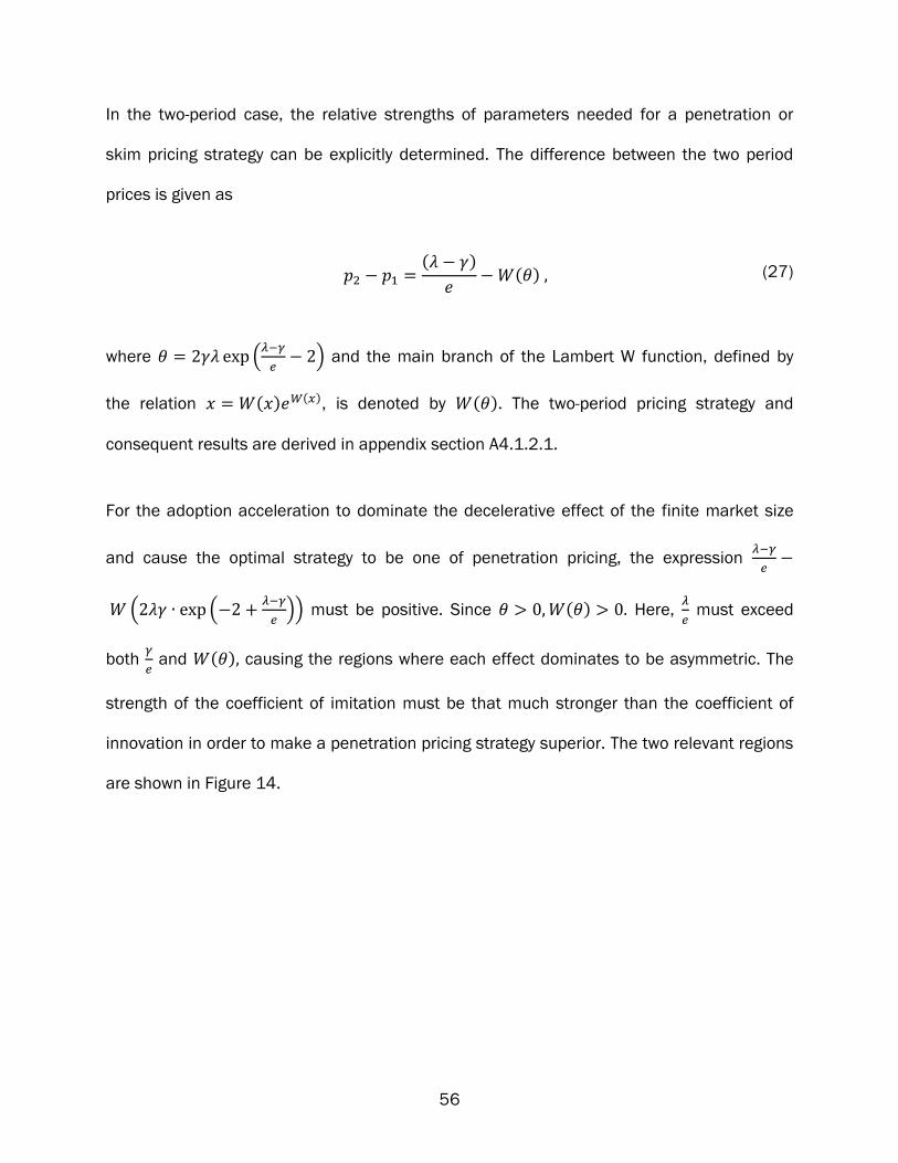
56

In the two-period case, the relative strengths of parameters needed for a penetration or

skim pricing strategy can be explicitly determined. The difference between the two period

prices is given as

( )

( ) (27)

where (

) and the main branch of the Lambert W function, defined by

the relation ( ) ( ), is denoted by ( ). The two-period pricing strategy and

consequent results are derived in appendix section A4.1.2.1.

For the adoption acceleration to dominate the decelerative effect of the finite market size

and cause the optimal strategy to be one of penetration pricing, the expression

( (

)) must be positive. Since ( ) Here,

must exceed

both

and ( ) causing the regions where each effect dominates to be asymmetric. The

strength of the coefficient of imitation must be that much stronger than the coefficient of

innovation in order to make a penetration pricing strategy superior. The two relevant regions

are shown in Figure 14.

57

Figure 14: Two Period Pricing Strategy

The boundary of the region where adoption acceleration dominates is found by solving the

equation

( (

)) for Using this solution, we conclude that

the firm uses a penetration pricing strategy when

.

There is an absolute boundary for this region given by

. When meets or

exceeds

then no matter the strength of the coefficient of imitation, , a price skimming

strategy is optimal. If the effect of the advertising channel is especially strong, then the firm

has no need to encourage adoption by charging a lower price in the first period to increase

demand in the second period.

58

4.3.3 Effect of the Diffusion Mechanism

The diffusion mechanism provides a potential reason for the firm to produce less than the

fully optimal production level of the purchase delay model because there is a positive effect

of adoption. The firm makes greater profits overall by encouraging market adoption, even if

the per-period profit is lower in the early periods. Table 6 summarizes the optimal production

levels for the diffusion by contagion and the purchase delay models.

When the diffusion effect, ∑ , is less than one, the production level is less than

that of the purchase delay model for an equivalent market adoption rate. The production

level for an equivalent adoption rate is lower because the value of the term

( ∑ ) ( ∑

∑

) is identical in both models and the value of

(∑

∑

) is between zero and one.

Table 6: Effect of the Diffusion Mechanism on Optimal Production

Optimal Production Levels

Diffusion by Contagion

( ∑

) ( ∑

( ∑ )

)( ∑

) ( ∑

( ∑ )

)

Purchase Delay

( ∑

) ( ∑

( ∑ )

)

Figure 15 illustrates the effect of the diffusion mechanism for parameter pairs where the

diffusion effect is less than one. The production levels are all lower than the optimal

production levels for pure purchase delay.

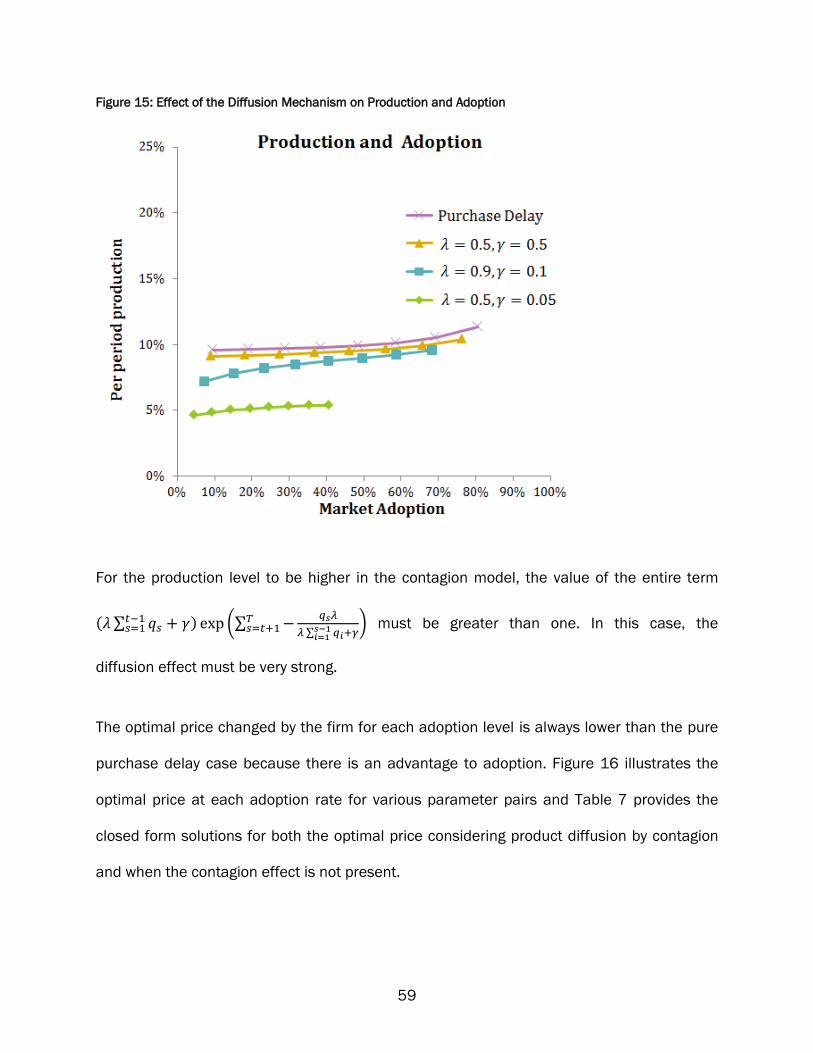
59

Figure 15: Effect of the Diffusion Mechanism on Production and Adoption

For the production level to be higher in the contagion model, the value of the entire term

( ∑ ) (∑

∑

) must be greater than one. In this case, the

diffusion effect must be very strong.

The optimal price changed by the firm for each adoption level is always lower than the pure

purchase delay case because there is an advantage to adoption. Figure 16 illustrates the

optimal price at each adoption rate for various parameter pairs and Table 7 provides the

closed form solutions for both the optimal price considering product diffusion by contagion

and when the contagion effect is not present.

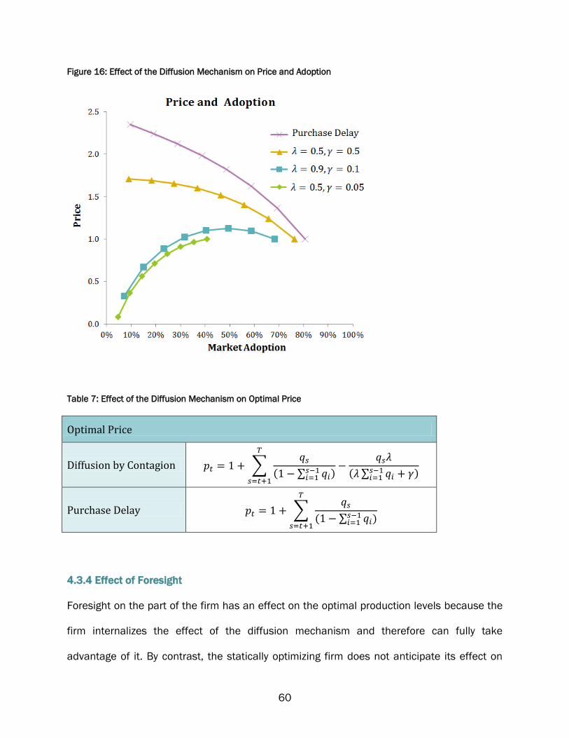
60

Figure 16: Effect of the Diffusion Mechanism on Price and Adoption

Table 7: Effect of the Diffusion Mechanism on Optimal Price

Optimal Price

Diffusion by Contagion ∑

( ∑ )

( ∑ )

Purchase Delay ∑

( ∑ )


Foresight on the part of the firm has an effect on the optimal production levels because the

firm internalizes the effect of the diffusion mechanism and therefore can fully take

advantage of it. By contrast, the statically optimizing firm does not anticipate its effect on

61

adoption and makes a lower total profit. Table 8 provides a comparison of the fully optimal

production and price level to the static optimization solutions. The static optimization

solution is derived in appendix section A4.3.3.

Table 8: Effect of Foresight on Optimal Production Level and Price

Production level

Fully Optimal

( ∑

)( ∑

) ( ∑

( ∑ )

( ∑ )

)

Static Optimization

( ∑

)( ∑

)

Price

Fully Optimal ∑

( ∑ )

( ∑ )

Static Optimization

The production levels in these two cases differ by the multiplicative factor

( ∑

∑

∑

) (28)

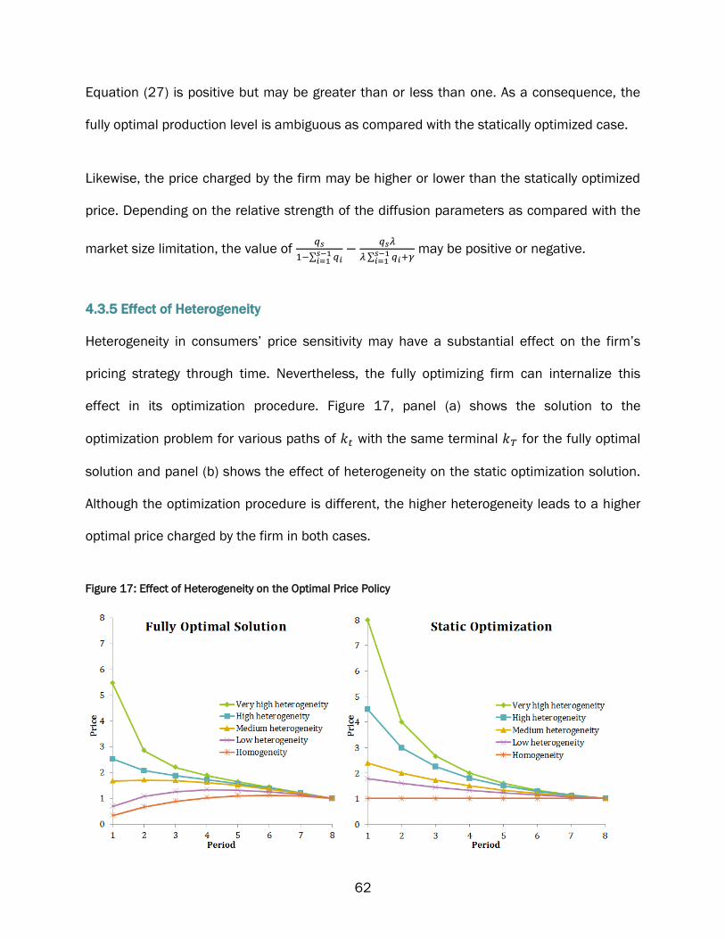
62

Equation (27) is positive but may be greater than or less than one. As a consequence, the

fully optimal production level is ambiguous as compared with the statically optimized case.

Likewise, the price charged by the firm may be higher or lower than the statically optimized

price. Depending on the relative strength of the diffusion parameters as compared with the

market size limitation, the value of

∑

∑

may be positive or negative.


Heterogeneity in consumers’ price sensitivity may have a substantial effect on the firm’s

pricing strategy through time. Nevertheless, the fully optimizing firm can internalize this

effect in its optimization procedure. Figure 17, panel (a) shows the solution to the

optimization problem for various paths of with the same terminal for the fully optimal

solution and panel (b) shows the effect of heterogeneity on the static optimization solution.

Although the optimization procedure is different, the higher heterogeneity leads to a higher

optimal price charged by the firm in both cases.

Figure 17: Effect of Heterogeneity on the Optimal Price Policy

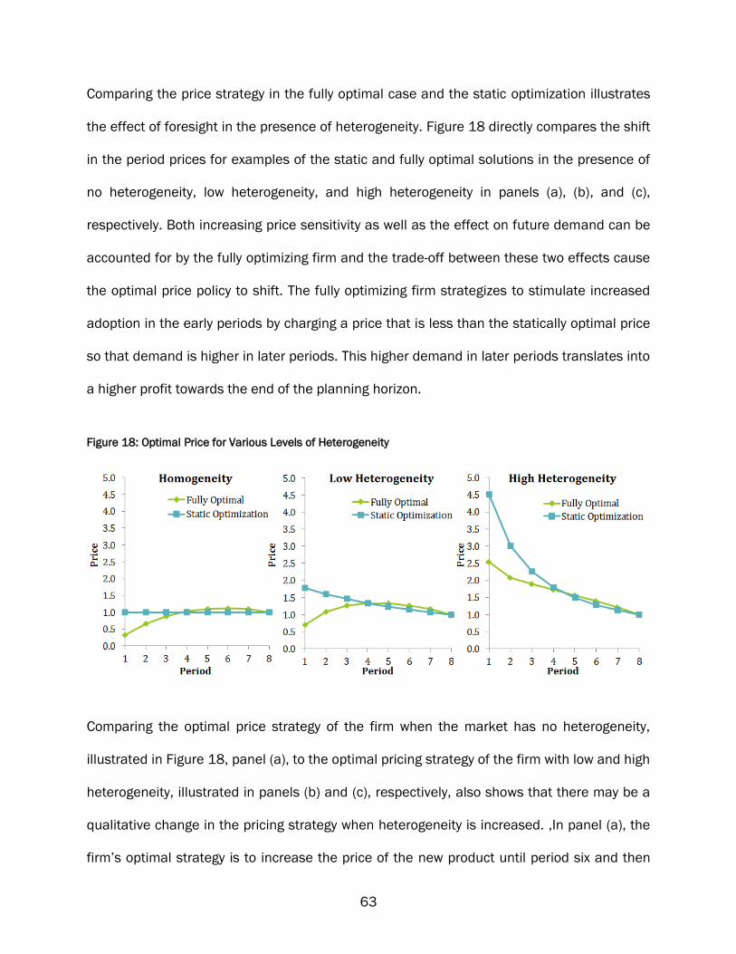
63

Comparing the price strategy in the fully optimal case and the static optimization illustrates

the effect of foresight in the presence of heterogeneity. Figure 18 directly compares the shift

in the period prices for examples of the static and fully optimal solutions in the presence of

no heterogeneity, low heterogeneity, and high heterogeneity in panels (a), (b), and (c),

respectively. Both increasing price sensitivity as well as the effect on future demand can be

accounted for by the fully optimizing firm and the trade-off between these two effects cause

the optimal price policy to shift. The fully optimizing firm strategizes to stimulate increased

adoption in the early periods by charging a price that is less than the statically optimal price

so that demand is higher in later periods. This higher demand in later periods translates into

a higher profit towards the end of the planning horizon.

Figure 18: Optimal Price for Various Levels of Heterogeneity

Comparing the optimal price strategy of the firm when the market has no heterogeneity,

illustrated in Figure 18, panel (a), to the optimal pricing strategy of the firm with low and high

heterogeneity, illustrated in panels (b) and (c), respectively, also shows that there may be a

qualitative change in the pricing strategy when heterogeneity is increased. ,In panel (a), the

firm’s optimal strategy is to increase the price of the new product until period six and then

64

decrease it until the end of the planning horizon. Panel (b) shows a similar strategy when

there is a low amount of heterogeneity. The fully optimizing firm increases the price until

approximately mid-way through the planning horizon, and then begins to decrease it for the

remainder. By contrast, panel (c) shows an optimal strategy of pure price skimming—the firm

decreases the price in each subsequent period for all eight periods.

The finding illustrated in Figure 18—that increasing heterogeneity may dominate the

adoption effect and cause a skim pricing strategy to be optimal when a penetration pricing

strategy was optimal in the homogeneous case—can be derived more generally. The period-

by-period price for the general solution is given by

(

( ∑ ) ( ∑

)

( ∑ )( ∑

)

) (29)

The pricing strategy shown in equation (29) is derived in appendix section A4.3.2.2. There

are two effects of a change in the ratio

, which describes the relative heterogeneity.

First, an intercept effect caused by the linear term

and second, a curvature effect via

the impact of

on the production levels in earlier periods, . The coefficient

can be thought of as a scaling factor that never affects the pricing strategy qualitatively

but affects the size of the price change period-by-period.

The nature of the curvature effect can be seen by examining the two-period case, which,

along with the consequent results in this section, are derived in appendix section A4.1.2.2.

The pricing strategy can be explicitly determined as

65

(

( )

( )) (30)

where

(

) and the main branch of the Lambert W function is

denoted by ( ).

Parallel to the general case, there are two effects of an increasing

: an effect on the

function’s intercept and an effect on the function’s curvature through the term

( ).

The curvature effect can be either positive or negative in

The derivative of ( ) with

respect to the relative heterogeneity,

is

( )

( ) (

)

(( )

)

( )

( ( )) (31)

Since ( ) and so ( )

( ) . The term (

)

is greater than zero as well.

However,

may be positive or negative, and thus its effect may be to increase or

decrease the difference in successive periods’ prices.

The curvature effect is shown in Figure 19 for various parameter values. Panel (a) illustrates

this effect when the parameters and are equal, while panel (b) shows that the curvature

effect when the parameters are not equal, illustrating that the derivative may change signs.

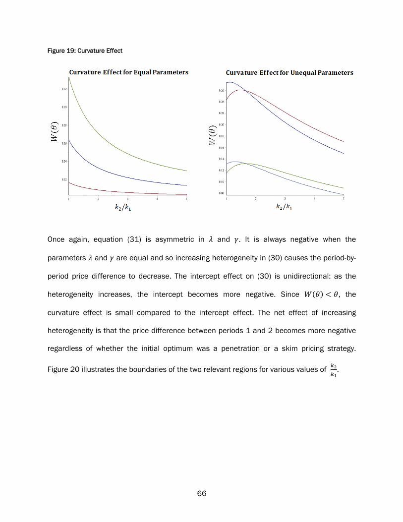
66

Figure 19: Curvature Effect

Once again, equation (31) is asymmetric in and . It is always negative when the

parameters and are equal and so increasing heterogeneity in (30) causes the period-by-

period price difference to decrease. The intercept effect on (30) is unidirectional: as the

heterogeneity increases, the intercept becomes more negative. Since ( ) , the

curvature effect is small compared to the intercept effect. The net effect of increasing

heterogeneity is that the price difference between periods 1 and 2 becomes more negative

regardless of whether the initial optimum was a penetration or a skim pricing strategy.

Figure 20 illustrates the boundaries of the two relevant regions for various values of

.

67

Figure 20: Pricing Strategy Boundary for Various Levels of Heterogeneity

The heterogeneity effect can dominate any set of parameters and so that the second

period price exceeds the first period price because there is a value of

that causes the

term

to be negative for any chosen values of and Regardless of how strong the

effect of adoption is on demand in future periods, a very large amount of heterogeneity will

cause the increasing price sensitivity in the market to dominate. Thus, the optimal strategy

will be one of skim pricing.

68

For a given ratio

the region where penetration pricing is optimal is bounded by

(

)

. There is a maximum for this expression since

. Even as heterogeneity

increases, is still ultimately bounded by

. This means that if

, heterogeneity

can never be reduced enough in order for a penetration pricing strategy to be optimal. This

region is coloured in blue in Figure 21. The interpretation of this result is that the coefficient

of innovation, , is high enough that there are always enough willing adopters in the second

period for the firm to benefit. The firm does not need to encourage adoption by charging a

lower price in the first period and prefers to take advantage of the lower price sensitivity in

the first period due to the high heterogeneity by following a skim pricing strategy.

Since

(

)

, there always exists a region where the optimal

pricing strategy is for penetration pricing even as the heterogeneity approaches infinity. This

region is coloured in pink in Figure 21. This means that, regardless of the amount of

heterogeneity, a parameter pair can be found for which a penetration pricing strategy is

optimal. If the coefficient of innovation, , is very low, the firm is then forced to use an

aggressive penetration pricing strategy in the first period in order to have any demand at all

in the second period. The benefit of having increased adoption in the second period

outweighs the advantage of the lower price sensitivity due to high heterogeneity among

adopters in the first period.

69

Figure 21: Pricing Strategy Regions in the Presence of Heterogenity

4.4 Conclusions

The results of the preceding model mirror the elegant results of Robinson and Lakhani

(1975) who investigate several common pricing rules and compare them with a fully

dynamic model where the firm anticipates its effect on adoption. They show that a firm that

anticipates a new product to be adopted dynamically has a higher overall profit than one

with a pricing strategy based on a static optimization: “Planning based on the dynamic

models can lead to a significant improvement in long run profit performance” (Robinson and

Lakhani, 1975, p. 1122). The analysis of the preceding model shows the same result.

However, because the profit necessarily begins at a lower value, the firm must again be

70

prepared to substitute present profits in order to benefit in future periods. The sentiment of

this cautionary result is consistent with Robinson and Lakhani’s advisory: “In a market with

growth potential, even a monopolist, motivated by nothing but a desire for high profits in the

long run, should follow surprisingly aggressive pricing strategies characterized by the

absorption of sizeable losses during a significant fraction of the initial planning period”

(p. 1122).

The optimal strategy of a firm launching a new product for which diffusion is effectively

modelled by contagion can take one of three forms:

Complete price skimming—the optimal strategy may be a decreasing price policy

throughout the planning horizon.

Complete penetration pricing—it may be optimal for the firm to increase prices

throughout the planning horizon.

A period of penetration pricing followed by a period of price skimming—the firm may

be better off beginning by increasing the price and then beginning to decrease it

again towards the end of the planning horizon.

In terms of the pricing strategy, the base case of the model of Subsection 4.3 agrees with

Kalish’s (1985) model which has a completely continuous pricing and sales path with

separable demand and diffusion functions. He writes, “This result implies that optimal price

increases as long as additional sales increase future demand, and vice versa. In other

words, for a period of positive effects of sales on demand, price is initially low to stimulate

early adopters, which in turn will stimulate demand. Price will monotonically increase to the

point where this 'word-of-mouth' effect diminishes. On the other hand, if there is a negative

71

effect of sales now on subsequent demand, price is initially relatively high, skimming more

profits from those who are willing to pay for early adoption, decreasing monotonically over

time” (Kalish, 1985, pp. 143–144).

However, the results contrast with Bass and Bultez (1982) whose analysis shows a pricing

strategy that is monotonically decreasing. The discrepancy is due to the interaction of price

and demand in the present model. Bass and Bultez assume that the evolution of demand is

independent of price. Thus, the firm is not able to internalize both the price and the demand

effect in their optimization and, consequently, the prediction differs.

The firm can decide which strategy to follow by considering the following questions:

1. Is there strong heterogeneity in price sensitivity in the market?

If there is a lot of diversity in price sensitivity in the market, then the firm may employ

a price skimming strategy to take advantage of the less price-sensitive consumers at

the beginning of the planning horizon. They would prefer to serve the “up-market”—

those with lower price sensitivity.

2. Is the contagion effect strong?

If the effect of other adopters on new consumers is strong, then a penetration pricing

strategy should be followed. This would most likely be for goods that are easily

apparent—like ice cream in a park. Conversely, if consumers are only weakly affected

72

by other adopters, then a skim pricing strategy is better—for example, something that

is not socially shared or made public.

3. Do we expect competitive entry before a majority of consumers have adopted?

If the firm anticipates competitive entry before a majority of consumers have

adopted, the firm must decide on its pricing strategy based on the strength of the

adoption and advertising parameters. If no competitive entry is expected before a

majority have adopted, the firm must expect that its pricing policy must begin to

decrease when the market saturation has reached 50 percent. Once that half-way

point has been reached, there is no longer any reason for the firm to be increasing

their price period-by-period.

73

CHAPTER 5: DIFFUSION BY SOCIAL INFLUENCE

5.1 Social Influence as a Diffusion Mechanism

A product that a firm wishes to introduce may carry a social risk to its adoption. An individual

may be apprehensive about adopting the product before others do so because going against

the social norm may be perceived as risky by the consumer. Fashion trends in apparel are

among the most obvious examples of products in this class. An individual consumer may not

wish to adopt a fashion trend until a certain number of others have already begun to dress

in a certain way. Products that imply certain values by their adoption on the part of the

consumer also have a social component, such as curb-side recycling programs, hybrid or

electric cars, and energy efficient light bulbs. Because adoption implies values or beliefs on

the part of the consumer, an individual may not wish to adopt a product until he or she is

sure that the value the product implies is common enough among their peers to be socially

acceptable.

Social influence, a diffusion mechanism explored by Schelling (1971; 1978), Henrich

(2001), and others, has been used as such not only for product adoption but also for

behavioural change. It has been applied to sociological research areas such as voting,

rioting, and migration (Granovetter, 1978). The aforementioned sociological research

suggests that adoption occurs due to a desire for social conformity. Individuals assess the

risk of making one decision versus another based on what others are doing. The activity in

question may be quite risky to do on one’s own (rioting, for example) or much less risky

(such as trying out a new brand of soup). Product adoption is therefore considered to be a

behavioural decision of this type. Consumers adopt a product upon seeing that a certain

74

level of adoption has been met in the population as a whole. This threshold is specific to

each potential adopter. When the market adoption exceeds the individual’s threshold, they

will be willing adopt the product. An interesting consequence is a possible adoption of a sub-

optimal or undesirable result (Bikhchandani, 1992, for instance).

The firm’s optimization problem is analogous to that of the workplace slo-pitch team

captain. When the sign-up sheet is first posted, only a few people who really like slo-pitch

join the team. Then, those who didn’t want to be the first to sign up, but are interested, sign

up. But after that, few may be willing to sign up. The slo-pitch team captain may do better by

incenting a few people to sign up in the early stages so that others see that many have

already sign up. Then those who see that quite a few people have signed up and who don’t

want to be left out of the water-cooler conversations also put their name down. Thus the

team captain can ensure a good turn-out by, perhaps, subsidizing the fee for the first few

sign-ups to ensure that the total contributions collected can cover the cost of new uniforms.

The firm’s decision problem is the same: ensure that there are enough adopters within the

population in the early stages so that others perceive that the behaviour is not socially risky,

and thus are encouraged to adopt.

This model proposes that new product adoption is risky to the consumer because adoption

may go against the social norm. This assumption suggests that any product that is privately

consumed and thus unseen by others would not be captured by the following framework.

5.2 Model Framework

Let ( ) and ( ) be the probability density function and cumulative distribution of the social

thresholds in the consumer population, respectively. We assume that ( ) is continuous to

75

enable general analysis. The function ( ) represents the distribution of adoption

requirements needed for consumers to be willing to adopt at each adoption rate . Then,

( ) represents the total proportion of thresholds that have been crossed at the adoption

rate . Once the threshold is reached they have a certain probability of adopting in that

period, which captured by the time-dependent fraction . For the adoption to get off the

ground there must be a non-zero proportion of early adopters who have a social threshold of

zero—they will adopt even if no one else adopts. Formally, this means that ( ) If

( ) , all consumers are innovators whose threshold is zero. In this case, the model

reduces to pure purchase delay as discussed in Chapter 3. Since ( ) the adoption

rate will always be less than that of the inertia case, given an equivalent price path.

Therefore, the difference ( ) is the proportion of adopters who have had their

thresholds crossed in period and is the proportion of individuals left

to adopt. This means that the aggregate of the individual probabilities of adoption is given

as

( ) ( )

(32)

Therefore, price-independent adoption is given by

( )

( )

(33)

which, since simplifies to

76

( ( ) ) (34)

Equation (34) describes the maximum adoption if the good were available at no cost. Taking

into account price-sensitivity and using the fact that , the market-wide

demand is given as

( ) ( ) ( ( ) ) (35)

Solving (35) for price and using the fact that ∑ yields the following formula for

inverse demand:

(

( (∑ ) ∑

)

) (36)

As a result, the firm solves the following maximization problem for the -period planning

horizon:

{∑

(

( (∑ ) ∑

)

)

} (37)

5.2.1 Heterogeneity

This model has three different types of heterogeneity: (i) diversity due to price sensitivity, ,

(ii) diversity due to the possibility of purchase delay, and (iii) diversity due to the

distribution of social thresholds, ( ).

77

We are assuming that the two heterogeneity factors, ( ) and are independent.

However, this assumption may not be appropriate. Consumer research suggests that early

adopters—those who have low social thresholds and who are willing to adopt when there are

few or no other adopters—may also be less price sensitive (Tellis, 1988).

The factor does not affect the optimal price set by the firm and so is ignored in the

analysis in favour of considering the effect of heterogeneity parameter, , only.

5.2.2 Constraints on Production

In each period, there is a maximum production level corresponding to the case where the

price level is zero:

(∑

) ∑

(38)

Therefore, the firm may not be able to produce its desired level in each period.



Solutions for an eight-period optimization problem with various distributions of social

thresholds are shown in Figures 22, 23, and 24. These solutions are numerically and

theoretically derived in appendix section A5.2.

78

Figure 22: Optimal Eight-Period Solution for Uniformly Distributed Thresholds (1)

In the first example of a uniform distribution of social thresholds, the firm’s optimal pricing

strategy, which is depicted in panel (b), increases until period six and then decreases in the

last two periods of the planning horizon. Optimal production levels are shown in panel (a)

along with total adoption in each time period. The per-period profit and cumulative profit

made by the firm is given in panel (c). Per-period profit increases slightly until period six and

then declines for the remaining two periods.

Figure 23: Optimal Eight-Period Solution for Uniformly Distributed Thresholds (2)

79

In contrast to the optimal solution depicted in Figure 22, Figure 23 shows an example where

the firm’s optimal pricing strategy is to decrease the price it charges throughout the planning

horizon for uniformly distributed thresholds. The optimal production levels and total

adoption in each period are shown in panel (a). Optimal production increases throughout the

planning horizon. The optimal pricing strategy is for skim pricing throughout the entire

planning horizon, as shown in panel (b). Per-period and cumulative profit are shown in panel

(c). In this example, the firm’s per-period profit decreases throughout the entire planning

horizon.

Figure 24: Optimal Eight-Period Solution for Normally Distributed Thresholds

Figure 24 illustrates an example of an optimal solution when the social thresholds of the

population are normally distributed and the firm optimizes over eight periods. In the optimal

situation, the firm produces at levels depicted in panel (a). The production level is not

monotonic in this example: the firm’s optimal production in period two decreases but then

increases throughout the remainder of the eight periods. The optimal pricing policy

increases until period five and then decreases until the end of the planning horizon, as

shown in panel (b). Panel (c) shows the profit made by the firm in each period as well as

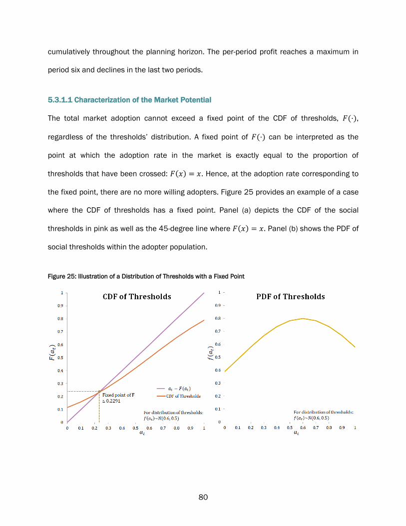
80

cumulatively throughout the planning horizon. The per-period profit reaches a maximum in

period six and declines in the last two periods.

5.3.1.1 Characterization of the Market Potential

The total market adoption cannot exceed a fixed point of the CDF of thresholds, ( ),

regardless of the thresholds’ distribution. A fixed point of ( ) can be interpreted as the

point at which the adoption rate in the market is exactly equal to the proportion of

thresholds that have been crossed: ( ) . Hence, at the adoption rate corresponding to

the fixed point, there are no more willing adopters. Figure 25 provides an example of a case

where the CDF of thresholds has a fixed point. Panel (a) depicts the CDF of the social

thresholds in pink as well as the 45-degree line where ( ) . Panel (b) shows the PDF of

social thresholds within the adopter population.

Figure 25: Illustration of a Distribution of Thresholds with a Fixed Point

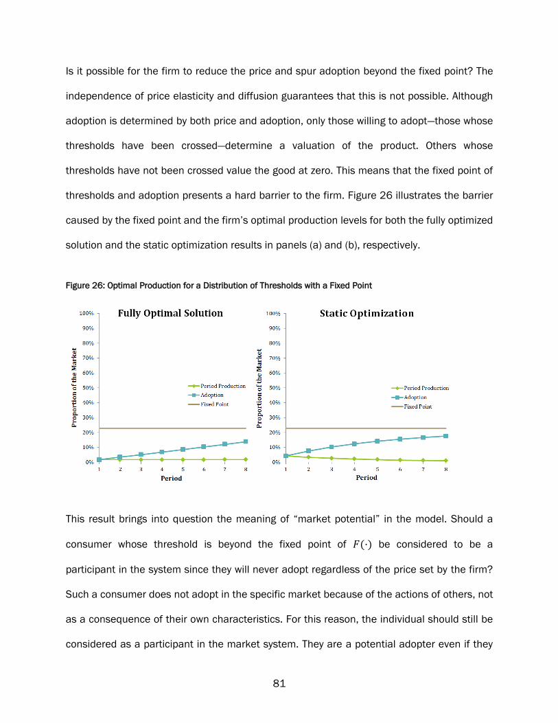
81

Is it possible for the firm to reduce the price and spur adoption beyond the fixed point? The

independence of price elasticity and diffusion guarantees that this is not possible. Although

adoption is determined by both price and adoption, only those willing to adopt—those whose

thresholds have been crossed—determine a valuation of the product. Others whose

thresholds have not been crossed value the good at zero. This means that the fixed point of

thresholds and adoption presents a hard barrier to the firm. Figure 26 illustrates the barrier

caused by the fixed point and the firm’s optimal production levels for both the fully optimized

solution and the static optimization results in panels (a) and (b), respectively.

Figure 26: Optimal Production for a Distribution of Thresholds with a Fixed Point

This result brings into question the meaning of “market potential” in the model. Should a

consumer whose threshold is beyond the fixed point of ( ) be considered to be a

participant in the system since they will never adopt regardless of the price set by the firm?

Such a consumer does not adopt in the specific market because of the actions of others, not

as a consequence of their own characteristics. For this reason, the individual should still be

considered as a participant in the market system. They are a potential adopter even if they

82

do not adopt within the specific market system. If this consumer were to be in another

population whose thresholds were distributed in a different way, they may adopt.

Consequently, adoption traps are possible for the class of products. If the social thresholds

are considered fixed, then the firm has no recourse: it is not able to bring about full adoption

of its product.

5.3.1.2 Pricing Constraints

In present model, the firm may have such a high desire to spur adoption to take advantage

of future demand that it may wish to push the upper bound of the feasible adoption level.

For example, in the first period, at the point where crosses the value of the initial

distribution of thresholds, the firm has hit the lower boundary. It cannot produce at its

desired value but rather must produce at exactly ( ). Figure 27 shows an example of a

distribution of thresholds for which the firm reaches this boundary. In panel (a), the firm

never meets the production constraint—it is able to produce at the optimum level regardless

of the distribution mean, Meanwhile, panel (b) shows a situation where the firm may wish

to produce at a higher level as compared with the initial demand due to the crossed social

thresholds.

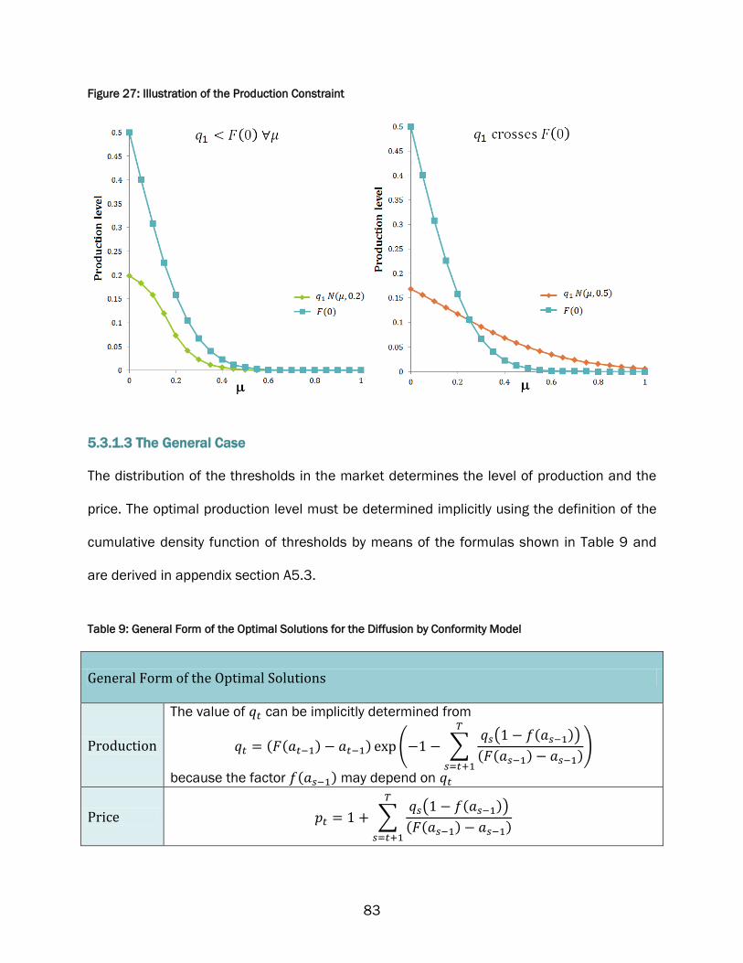
83

Figure 27: Illustration of the Production Constraint

5.3.1.3 The General Case

The distribution of the thresholds in the market determines the level of production and the

price. The optimal production level must be determined implicitly using the definition of the

cumulative density function of thresholds by means of the formulas shown in Table 9 and

are derived in appendix section A5.3.

Table 9: General Form of the Optimal Solutions for the Diffusion by Conformity Model


Production

The value of can be implicitly determined from

( ( ) ) ( ∑ ( ( ))

( ( ) )

)

because the factor ( ) may depend on

Price ∑ ( ( ))

( ( ) )

84

5.3.1.4 Normal Distribution

Respectively, the CDF and PDF of the normal distribution are given by

( )

(

√ )

(39)

and

( )

( )

( ( )

)

√

(40)

where the indicated error function, ( ), is defined in the conventional way as ( )

√ ∫

.

Table 10 shows the optimal production levels and price for normally distributed thresholds

with mean and standard deviation These results are derived in appendix section

5.3.1.3. The optimal production level must be implicitly determined for a specific distribution

and planning period length. Thus, few general conclusions are possible.

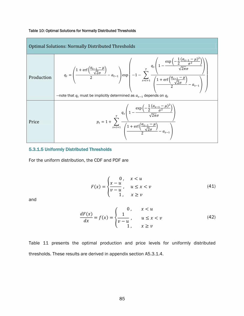
85

Table 10: Optimal Solutions for Normally Distributed Thresholds

Optimal Solutions: Normally Distributed Thresholds

Production (

(

√ )

)

(

∑

( (

( )

)

√ )

( (

√ )

)

)

—note that must be implicitly determined as depends on

Price ∑

( (

( )

)

√ )

( (

√ )

)

5.3.1.5 Uniformly Distributed Thresholds

For the uniform distribution, the CDF and PDF are

( ) {

(41)

and

( )

( ) {

(42)

Table 11 presents the optimal production and price levels for uniformly distributed

thresholds. These results are derived in appendix section A5.3.1.4.

86

If , then no thresholds are crossed, which means that there can be no adoption.

This case is impossible, so , including at zero. Therefore, This is a re-

statement of the condition that ( )

Table 11: Optimal Solutions for Uniformly Distributed Thresholds

Optimal Solutions: Uniformly Distributed Thresholds

Production

When ,

(

) ( ∑

(

)

( )

)

When ,

( ) ( ∑

)

Price

When ,

∑ (

)

When ,

∑


The pricing strategy depends on the PDF of thresholds, ( ), among potential adopters

since both and ( ) are positive. Specifically, when the PDF is greater than one,

the speed at which thresholds are being crossed is greater than the rate at which the

adoption is increasing. In this case, the optimal pricing strategy is for the price level to

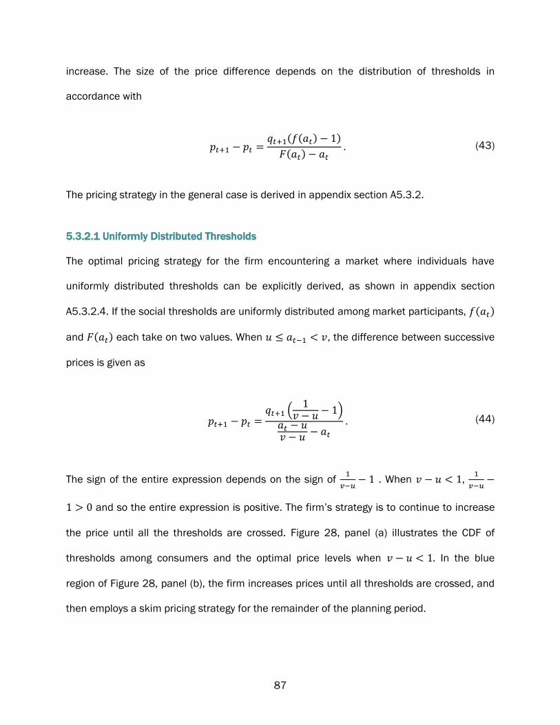
87

increase. The size of the price difference depends on the distribution of thresholds in

accordance with

( ( ) )

( ) (43)

The pricing strategy in the general case is derived in appendix section A5.3.2.

5.3.2.1 Uniformly Distributed Thresholds

The optimal pricing strategy for the firm encountering a market where individuals have

uniformly distributed thresholds can be explicitly derived, as shown in appendix section

A5.3.2.4. If the social thresholds are uniformly distributed among market participants, ( )

and ( ) each take on two values. When , the difference between successive

prices is given as

(

)

(44)

The sign of the entire expression depends on the sign of

. When ,

and so the entire expression is positive. The firm’s strategy is to continue to increase

the price until all the thresholds are crossed. Figure 28, panel (a) illustrates the CDF of

thresholds among consumers and the optimal price levels when In the blue

region of Figure 28, panel (b), the firm increases prices until all thresholds are crossed, and

then employs a skim pricing strategy for the remainder of the planning period.

88

Figure 28: CDF of Thresholds and Optimal Price Strategy when

When , fewer thresholds are being crossed with each adoption. This case is

depicted in Figure 29, panel (a). In this case, the firm’s strategy is to undertake skim pricing

in both regions, as seen in Figure 29, panel (b).

Although the firm uses a skim pricing strategy for both regions, the quantitative difference in

successive periods’ prices is lower before all thresholds are crossed. As the rate at

which thresholds are crossed approaches zero:

(

)

(45)

Equation (45) indicates that the optimum approaches that of the purchase delay model

studied in Chapter 3.

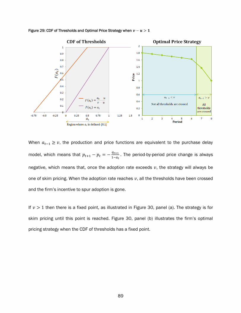
89


When , the production and price functions are equivalent to the purchase delay

model, which means that

. The period-by-period price change is always

negative, which means that, once the adoption rate exceeds , the strategy will always be

one of skim pricing. When the adoption rate reaches , all the thresholds have been crossed

and the firm’s incentive to spur adoption is gone.

If then there is a fixed point, as illustrated in Figure 30, panel (a). The strategy is for

skim pricing until this point is reached. Figure 30, panel (b) illustrates the firm’s optimal

pricing strategy when the CDF of thresholds has a fixed point.

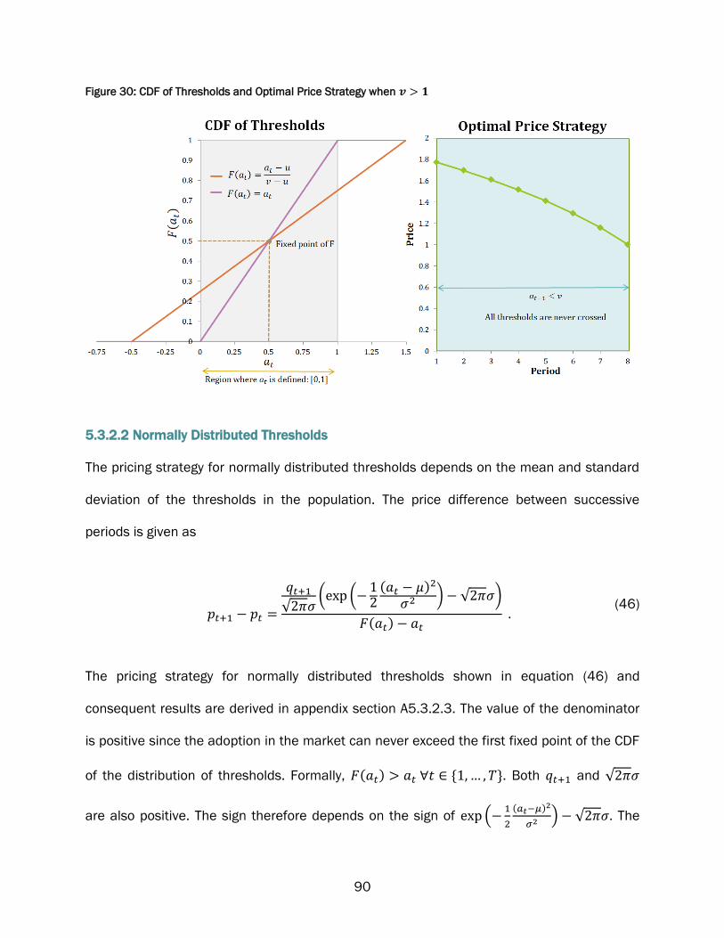
90


5.3.2.2 Normally Distributed Thresholds

The pricing strategy for normally distributed thresholds depends on the mean and standard

deviation of the thresholds in the population. The price difference between successive

periods is given as

√ ( (

( )

) √ )

( )

(46)

The pricing strategy for normally distributed thresholds shown in equation (46) and

consequent results are derived in appendix section A5.3.2.3. The value of the denominator

is positive since the adoption in the market can never exceed the first fixed point of the CDF

of the distribution of thresholds. Formally, ( ) . Both and √

are also positive. The sign therefore depends on the sign of (

( )

) √ The

91

value of (

( )

) is between zero and one because

( )

. This means that if

√ , the entire expression is negative for any In this case, the firm always

employs a skim pricing strategy:

When

√ , the firm has a penetration price strategy when , which means

that (

( )

) √ . Isolating this expression for | | we find that the pricing

strategy depends on the absolute difference between the adoption rate and the mean of

thresholds through the relation

| | √ ( ) (47)

Equation (47) is bounded. The expression √ ( ) achieves a maximum when

( √ ( ))

√ ( )

√ ( ) (48)

which occurs when

√ . This corresponds to | | √ ( )

√ . Therefore, the firm never has a penetration pricing strategy when the

absolute difference between the adoption rate and the mean is greater than | |

√ . The inequality in (47) describes an absolute value and so there are two situations that

satisfy this bound that may be interpreted in different ways. In the first case, if the adoption

rate is smaller than the mean of thresholds, the firm cannot reach the concentration of

thresholds near the mean to be able to benefit from the penetration pricing strategy. The

92

firm would have to forego so much profit to spur adoption that it would not be able to recoup

these foregone earnings in future periods. In the second case, the adoption rate may be

larger than the mean of thresholds by such a margin that crossing more thresholds does not

give enough momentum to benefit the firm in future periods.

Figure 31 illustrates the two regions in which the firm employs each pricing strategy. In the

two-period planning problem, the adoption rate at time is simple the adoption of the first

period, so Within the blue region, the optimizing firm starts by charging a lower price

and then increases it in the second period. For pairs of and in the green region, the

firm’s optimal strategy is to charge a higher price in the first period then lower it in the

second.

Figure 31: Two Period Pricing Strategy

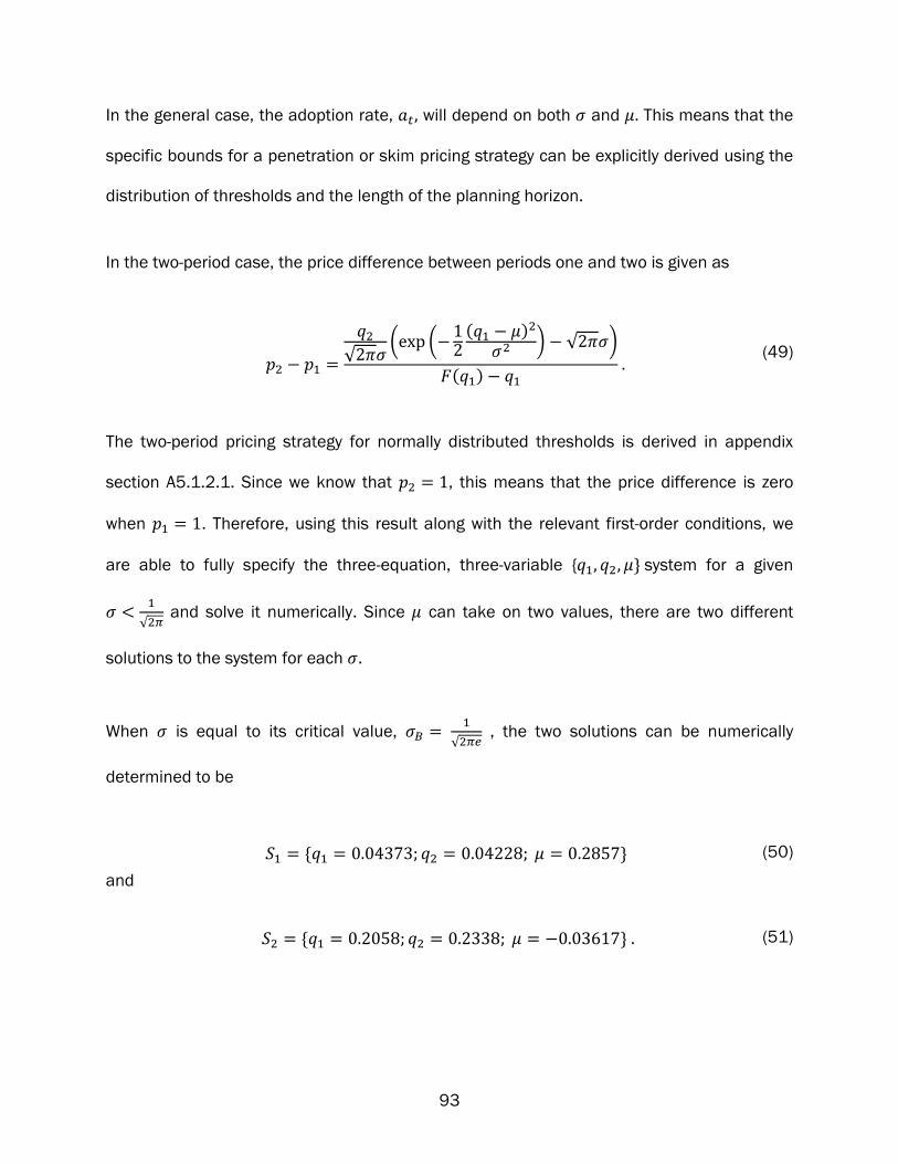
93

In the general case, the adoption rate, will depend on both and This means that the

specific bounds for a penetration or skim pricing strategy can be explicitly derived using the

distribution of thresholds and the length of the planning horizon.

In the two-period case, the price difference between periods one and two is given as

√ ( (

( )

) √ )

( )

(49)

The two-period pricing strategy for normally distributed thresholds is derived in appendix

section A5.1.2.1. Since we know that , this means that the price difference is zero

when . Therefore, using this result along with the relevant first-order conditions, we

are able to fully specify the three-equation, three-variable { system for a given

√ and solve it numerically. Since can take on two values, there are two different

solutions to the system for each .

When is equal to its critical value,

√ , the two solutions can be numerically

determined to be

(50)

and

(51)

94

The absolute difference between the adoption in period 1, and the mean, , in both

cases is

√ :

| | | | | | | |

√

(52)

These values represent the widest region where the firm’s best policy is a penetration

pricing strategy. Figure 32 illustrates the critical boundaries for the two-period case. Within

the blue region, a pricing strategy where the firm charges a lower price in the first period

compared to the second period is optimal. In the green regions, the firm’s optimal strategy is

to charge a higher price in the first period than the second period.

For any other value of larger or smaller than , the blue region in Figure 32 would be

narrower.

95

Figure 32: Pricing Strategy for the Two Period Case


The diffusion mechanism affects the optimal price and production levels. In the limit, it

reduces to the purchase delay model discussed in Chapter 3. When the CDF of thresholds is

distributed such that ( ) is one, the optima are identical in these two models. This

special case is interpreted as a population where all social thresholds are at zero—every

potential adopter does not require any prior adoption in the market to be willing to purchase

the product provided that the market price is lower than their reservation price.

In the general case, the specific production and price levels depend on the relative values of

the formulae shown in Table 12. The relative values of these solutions depend on the

distribution of thresholds and cannot be completely determined without an explicit

assumption regarding this distribution.

96

Table 12: Effect of the Diffusion Mechanism on Optimal Production Levels


Diffusion by Conformity

The value of can be implicitly determined from

( ( ) ) ( ∑ ( ( ))

( )

)

because the factor ( ) may depend on

Purchase Delay ( ) ( ∑

)

Optimal Price

Diffusion by Conformity

∑ ( ( ))

( )

Purchase Delay ∑


Foresight affects both the price and production levels of the firm but the direction of the

effect is ambiguous. Table 13 summarizes the optimal solutions for the fully optimized case

as well as the solution for the static optimization. The static optimization solutions are

derived in appendix section A5.3.3.

97

Table 13: Effect of Foresight on Optimal Production Levels


Fully Optimal ( ( ) ) ( ∑ ( ( ))

( )

)

Static Optimization

( ( ) )

Because of the interdependency of and ( ) for , the nature of the effect

cannot be determined without further assumptions on the distribution of ( ) Figure 33

provides an example showing regions where the production levels are higher as well as

regions where they are lower in the fully optimized solution as compared with the static

optimization. In panel (a), an example of the per-period production of an eight-period

planning horizon is shown against the total market adoption. The total adoption directly

determines the proportion of social thresholds that have been crossed, making the

production levels of the static and fully optimal solutions comparable. The per-period

production may be higher or lower at each adoption level in the static optimization as

compared with the fully optimal solution. Similarly, the per-period production in each period

in both solutions show no clear pattern, as illustrated in panel (b), which shows the same

eight-period solution. At various points, the optimal production levels of the fully optimal

solution may be higher or lower than those of the statically optimizing firm.

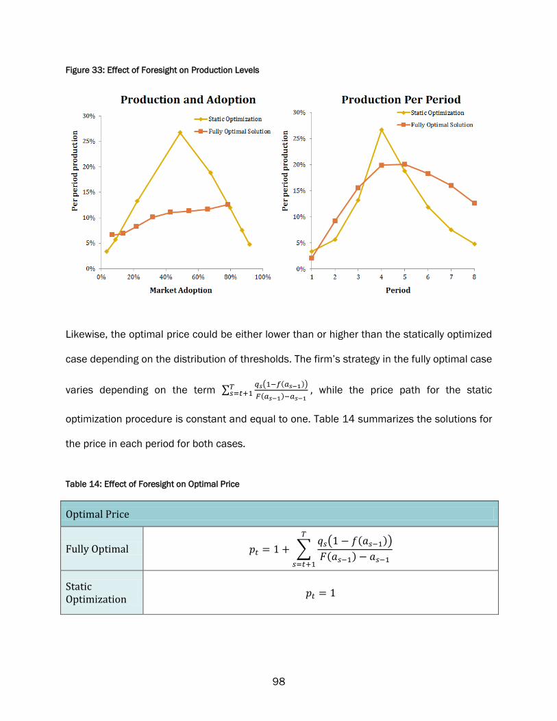
98

Figure 33: Effect of Foresight on Production Levels

Likewise, the optimal price could be either lower than or higher than the statically optimized

case depending on the distribution of thresholds. The firm’s strategy in the fully optimal case

varies depending on the term ∑ ( ( ))

( )

while the price path for the static

optimization procedure is constant and equal to one. Table 14 summarizes the solutions for

the price in each period for both cases.

Table 14: Effect of Foresight on Optimal Price

Optimal Price

Fully Optimal ∑ ( ( ))

( )

Static Optimization

99

The profit made by the firm is higher in the fully optimized case because the firm is able to

fully internalize its effect on the distribution of the consumers’ social thresholds. Although

the profit made by the statically optimizing firm begins at a higher level, the total profit for

the planning horizon is greater for the firm that fully optimizes by taking into account the

diffusion mechanism. Figure 34 shows an example of the per-period profit and the

cumulative profit made by the firm. Panel (a) shows the profit in each period for both firms.

The fully optimizing firm at times makes a lower profit per period as compared with the

statically optimizing firm. However, panel (b) shows that the total profit is unambiguously

greater for the fully optimizing firm.



When the population is heterogeneous due to their social threshold as well as their price

sensitivity, the optimal solution is affected. Heterogeneity of price sensitivity may therefore

change the pricing strategy. The optimal price policy for various levels of heterogeneity of

price sensitivity for both the fully optimizing firm and the static optimization is shown in

100

Figure 35. Panel (a) shows that, as this heterogeneity increases for the same terminal value,

the firm is more able to take advantage of the relatively lower price sensitivity in the earlier

periods. Thus, the optimal price charged by the firm is higher. This is also true when the firm

only optimizes statically, as shown in panel (b).

Figure 35: Effect of Heterogeneity on Price

The price strategy under heterogeneity depends on the ratio

. The value of

depends on this ratio directly as well as indirectly through its effect on , which is

determined by the distribution of thresholds. The general form of the pricing strategy under

heterogeneity is given by

(

( ( ))

( ) ) (53)

The general pricing strategy shown in equation (53) is derived in appendix section A5.3.1.2.

Since ( ( ) ) ( ∑ ( ( ))

( ( ) ) ) , the ratio

may have the

101

effect of either increasing or decreasing depending on the value of the terms containing

( ( ))

( ( ) ) Since ( ) depends on , there is an interdependency that cannot be

directly determined without further assumptions on the distribution ( )

5.4 Conclusions

Up until now, the consequences of modelling diffusion based on social conformity have not

been analyzed in terms of their impact on firms’ decisions but have rather been used to

explain diffusion in non-economic sociological contexts. However, the analysis in Subsection

5.3.4 clearly shows that a firm that can take these behavioural effects into account upon

launching a socially relevant product can benefit.

The optimal pricing strategy depends on the distribution of thresholds and may take any of

the following three forms:

Complete price skimming—it may be optimal for the firm to employ a decreasing price

policy throughout the planning horizon.

Complete penetration pricing—the firm’s best strategy may be to increase prices for

the entire planning horizon.

A combination strategy with skim pricing for part of the planning period and

penetration pricing for the remainder—the optimal strategy may be to increase prices

initially, but then decrease them in later periods.

The three different possibilities are similar to the results of Chapter 4. Quantitatively,

though, the character of the optimal period-by-period price changes differs. The explicit

102

formulations of the two models are based on different assumptions and therefore predict

differences in the shape of the adoption curve. This result is consistent with empirical

research which shows that not all adoption curves follow the same pattern.

Understanding the consumers’ thresholds is crucial to optimization in part because many of

the solutions cannot be determined in closed form. The optimal pricing strategy depends on

the rate at which potential adopters’ social thresholds are being crossed. Penetration pricing

is optimal if more thresholds are being crossed than adopters adopting. Once potential

adopters’ thresholds are being crossed more slowly, the firm’s strategy should be one of

skim pricing.

An aggressive pricing strategy is appropriate if there is a sub-group of low but non-zero social

thresholds and the diversity of thresholds is relatively small. The more homogenous the

thresholds, the more likely the penetration pricing strategy can have a positive effect.

Thresholds must be relatively homogenous and low, however, for this strategy to be optimal.

Misunderstanding of the social thresholds among adopters has the potential to be

devastating for a firm’s planning as there may be a point after which it cannot move

adoption. However, if the firm were able to predict this fixed point that there may be a

smaller market potential than anticipated, its planning could be improved. Numerous other

explanations have been given for adoption traps but the foregoing gives a very simple, but

unfortunately irresolvable, rationale.


103

1. On average, how many adopters would be needed encourage a particular potential

adopter to purchase?

If a large number of other adopters are required for many consumers to purchase, it is more

likely to be optimal to utilize a skim pricing strategy to benefit from the initially low price

sensitivity among early adopters. The firm must expect to have a relatively low overall

product adoption because relatively few new adopters’ thresholds are crossed with each

adoption.

2. Is there a wide diversity of social prerequisites in the adopter population?

If there is a broad range of social thresholds among the potential adopter population, it is

more likely that the firm will not be able to surpass enough potential adopter thresholds to

make a penetration pricing strategy optimal. For example, if the product in question has a

varied degree of importance within the potential adopter group due to attitudinal or

demographic factors. In this case, the firm should follow a skim pricing strategy.

3. Can the whole adopter population be encouraged to adopt?

This is perhaps the most important question for the firm to answer as the barrier inherent in

this model is impassable by a pricing strategy. The firm must endeavour to see whether the

population thresholds are such that the total adoption is bounded at some point less than

the full market potential.

104

CHAPTER 6: DIFFUSION BY INFORMATION

6.1 Value Uncertainty as a Diffusion Mechanism

Although many new products are incremental improvements to existing products with which

consumers are familiar, there are also products that create entirely new categories and have

little reference to existing products. So-called “new-to-the-world” products are described by

Bergstein and Estelami (2002) as follows:

New-to-the world products are innovative new products that due to their

unique attribute mix or technological features have provided leapfrogging

increases in consumer utility, to the point that new product categories have

emerged as a result of their introduction. Examples would be the Sony

Walkman (introduced in 1979), the 3M Post-it Notes (introduced in 1980),

and the first Xerox photocopier (introduced in 1952) (Bergstein and

Estelami, 2002, p. 303).

A firm wishing to launch this kind of product has a difficult task as consumers may have

difficulty fully understanding its the qualities and value. In this case, information may be

needed by consumers before they are willing to adopt. This information is provided by others

who have already adopted the product.

Although consumer electronics is often the first category to come to mind when thinking of

products for which information may be needed by potential adopters, many other types of

products may also have this requirement. A consumer may need to hear about ways in

which to incorporate a foreign food item into meals before they are willing to purchase it at

105

the grocery store. Alternatively, a consumer may need to read a certain number of reviews

on a new television show or book by a first-time writer before being willing to try it

themselves.

For this class of products, we can consider adoption as a signal that is observed by other

market participants. Each potential adopter has a certain threshold of information needed

before adopting and each adopter provides information about the desirability of the product

in every period beginning from the time that they first adopt. Essentially, the adopter

continues to discuss the adoption and so information accumulates in each period. This is

akin to an adopter showing and discussing their new purchase.

The adoption mechanism used in the following chapter has its roots in the economics

literature. In academic economics, various methods and motives for product adoption have

been advanced. Many associated models of adoption centre around the consumer’s

uncertainties about the characteristics of the product, which can only be inferred from

others’ adoptions of the product or upon adopting the product themselves in the manner

specified, for example, by Bikhchandani, Hirshleifer, and Welch (1992). Ellison and

Fudenberg (1995) also consider information generated by other adopters as influencing the

consumers’ decision-making but in relation to switching between the status-quo and a new

adoption. The framework developed by Bergmann and Valimaki (1997) suggests an initial

period of uncertainty both on the part of firms and on the part of consumers as to the value

of the new product. More recently, Hohnisch, Pittnauer, and Stauffer (2008) have used a

three-stage process of awareness, information, and adoption to establish diffusion. This

process supports a variety of approaches to modelling adoption. However, many models are

106

consistent with one another in that they assume an initial period of uncertainty on the part

of consumers that is remedied by adoption. This is the approach taken in comparing the

predictions of product diffusion to predictions made by the two processes outlined in

Chapters 3 and 5.

An advantage of this formulation for an adoption mechanism is its ability to explain

“percolation”—a period of slow growth in sales, or sometimes even a decline in sales,

followed by a sharp take-off—that has been observed in empirical research (Hohlnisch,

2008). The “percolation” occurs when information is being continuously generated by

adopters and accumulates until all of a sudden the thresholds of many potential adopters

are met. In this way, the adoption of the product may take off unexpectedly.

Any product for which information about its qualities or usage is irrelevant would not be a

good candidate for the model in this chapter. For example, if a product is quite simple, like

those considered in Chapter 4, the consumer is not likely to need any information before

being willing to adopt it.

6.2 Model Framework

Each potential adopter needs a certain amount of information about the product at hand to

decide whether or not to adopt. The probability density function of information needs is

denoted by ( ) and the cumulative distribution function of information needs is denoted

by ( ) We assume that ( ) is continuous. The function ( ) is the proportion of

consumers whose information needs are at least In each period , therefore, there is the

amount of information that has been generated in the past periods. Hence, there

are ( ) consumers willing to adopt. Note that the information generated is lagged by one

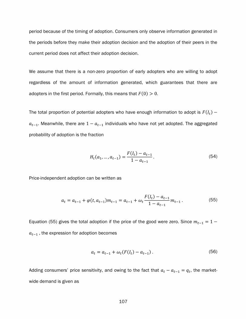
107

period because of the timing of adoption. Consumers only observe information generated in

the periods before they make their adoption decision and the adoption of their peers in the

current period does not affect their adoption decision.

We assume that there is a non-zero proportion of early adopters who are willing to adopt

regardless of the amount of information generated, which guarantees that there are

adopters in the first period. Formally, this means that ( )

The total proportion of potential adopters who have enough information to adopt is ( )

. Meanwhile, there are individuals who have not yet adopted. The aggregated

probability of adoption is the fraction

( ) ( )

(54)

Price-independent adoption can be written as

( )

( )

(55)

Equation (55) gives the total adoption if the price of the good were zero. Since

, the expression for adoption becomes

( ( ) ) (56)

Adding consumers’ price sensitivity, and owing to the fact that , the market-

wide demand is given as

108

( ) ( ) ( ( ) ) (57)

and solving for price yields inverse demand of

(

( ( ) ∑ )

) (58)

Therefore, the firm endeavours to solve the following -period planning problem:

{∑

(

( ( ) )

)

} (59)

6.2.1 Heterogeneity

Heterogeneity of consumers in this model is captured by three variables:

differences in informational needs to adopt, ( );

individual price sensitivity, ; and

the effect of possible delay of purchase, .

We assume that ( ) and are unrelated. There may in fact be a relationship between the

two, however, if ( ) is taken to represent informational needs. For instance, those who

have more education may have lower informational needs and also be more affluent, and

thus more willing to adopt regardless of the product’s price.

Once again, the parameter does not affect the firm’s price strategy, and so it is dropped

from the ensuing analysis.

109

6.2.2 Constraint on Production

As with the diffusion-by-conformity model discussed in Chapter 5, the firm may wish to

produce more in early periods to spur increased adoption in later periods. In doing so it is

constrained by the relation

( ) (60)

because there is a maximum number of consumers willing to adopt in any given period

regardless of the price level.

6.2.3 Information Generation

The variable represents the amount of information available to potential adopters at time

This depends on product adoption in all previous periods: is a function of .

There are numerous possible ways to formulate the information function. Herein we will use

the following criteria. Each adopter generates one equally valuable unit of information—

adoption itself is all that is relevant. The information generated in each period decays at a

rate , which means that only the fraction of the information is left in the next period.

Thus,

( ) ∑( )

∑( ) ∑

(61)

In the limiting case where , the information generated in previous periods decays

completely. Since ( ) ( ) , the information generated is equal to the total

proportion of adopters in the population:

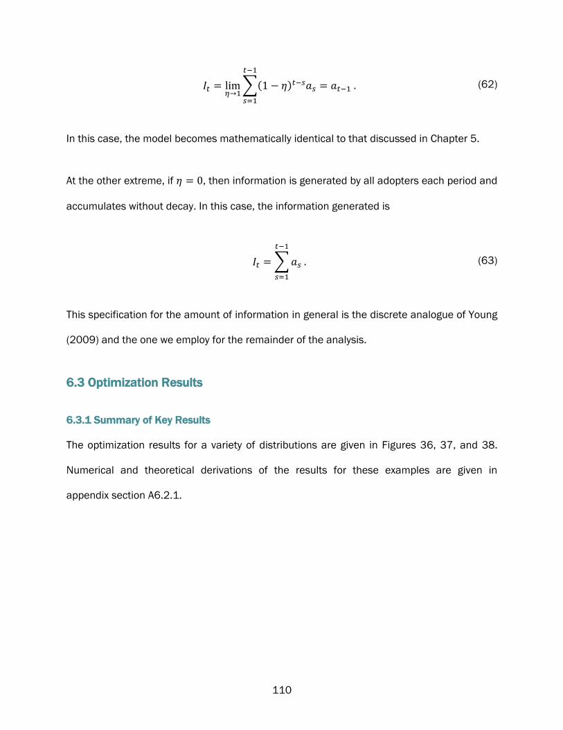
110

∑( )

(62)

In this case, the model becomes mathematically identical to that discussed in Chapter 5.

At the other extreme, if , then information is generated by all adopters each period and

accumulates without decay. In this case, the information generated is

∑

(63)

This specification for the amount of information in general is the discrete analogue of Young

(2009) and the one we employ for the remainder of the analysis.



The optimization results for a variety of distributions are given in Figures 36, 37, and 38.

Numerical and theoretical derivations of the results for these examples are given in

appendix section A6.2.1.

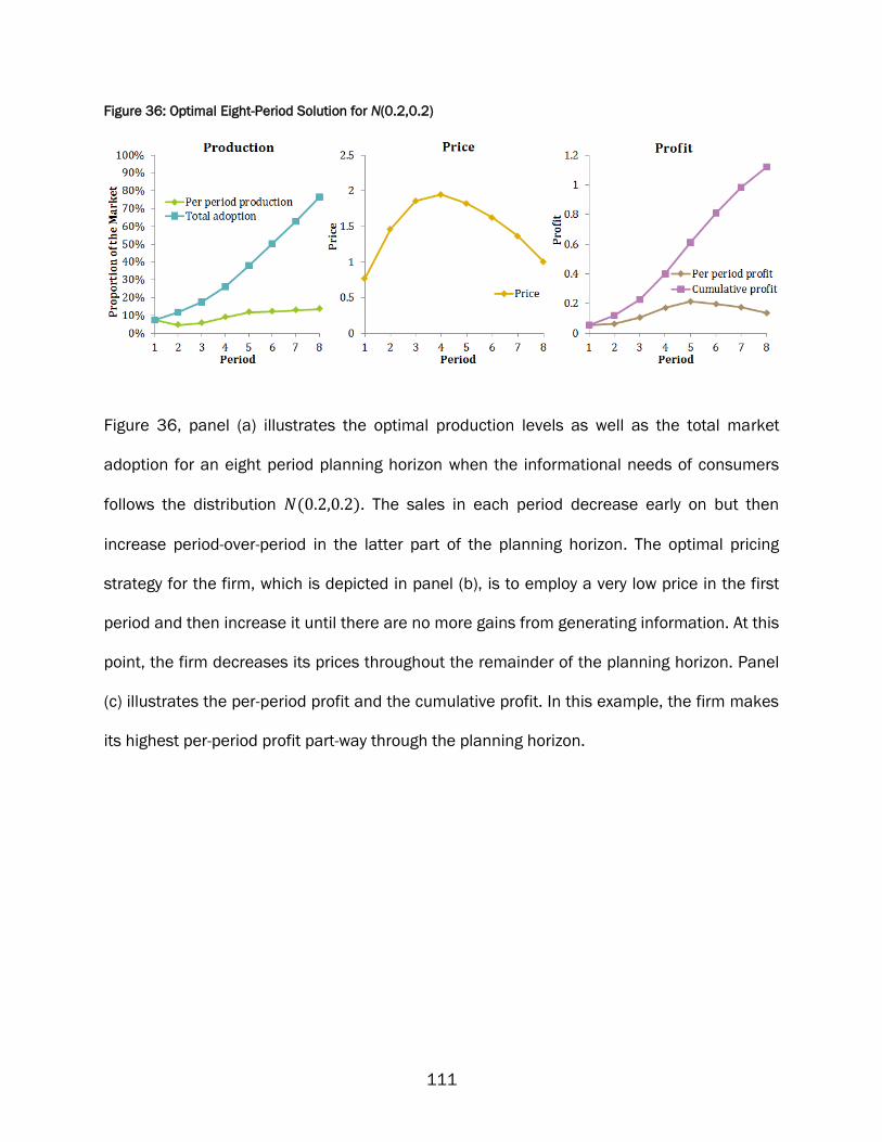
111

Figure 36: Optimal Eight-Period Solution for N(0.2,0.2)

Figure 36, panel (a) illustrates the optimal production levels as well as the total market

adoption for an eight period planning horizon when the informational needs of consumers

follows the distribution ( ). The sales in each period decrease early on but then

increase period-over-period in the latter part of the planning horizon. The optimal pricing

strategy for the firm, which is depicted in panel (b), is to employ a very low price in the first

period and then increase it until there are no more gains from generating information. At this

point, the firm decreases its prices throughout the remainder of the planning horizon. Panel

(c) illustrates the per-period profit and the cumulative profit. In this example, the firm makes

its highest per-period profit part-way through the planning horizon.

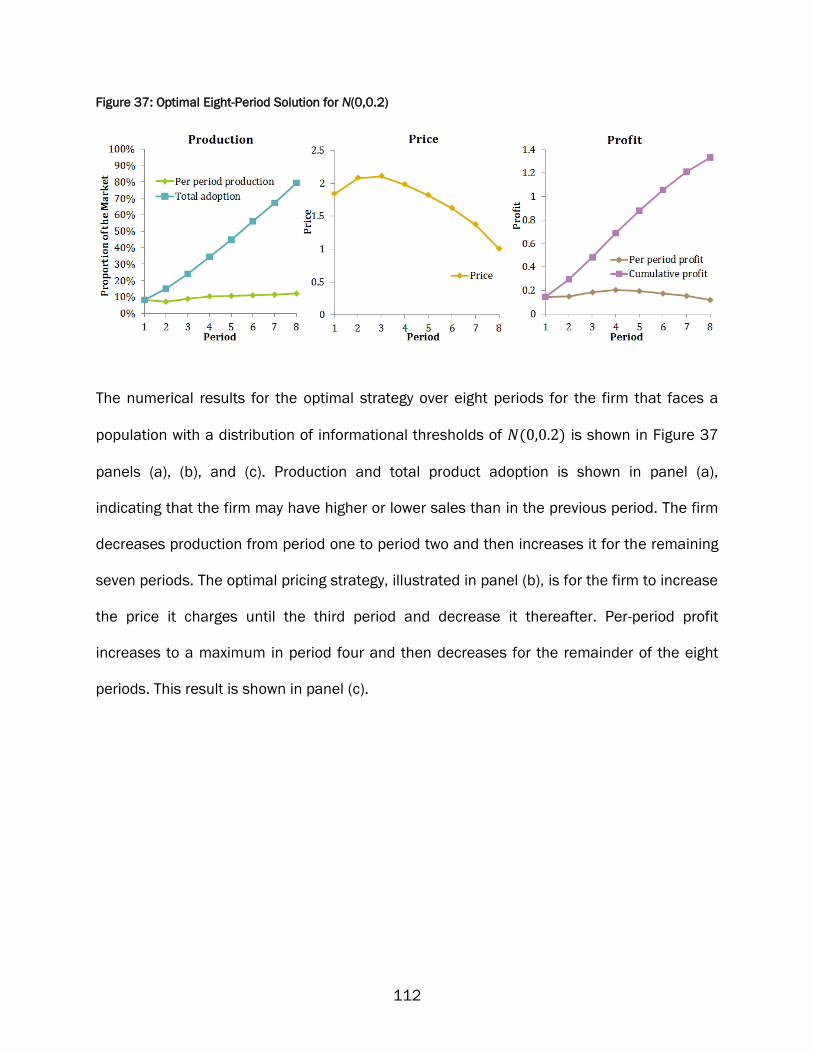
112

Figure 37: Optimal Eight-Period Solution for N(0,0.2)

The numerical results for the optimal strategy over eight periods for the firm that faces a

population with a distribution of informational thresholds of ( ) is shown in Figure 37

panels (a), (b), and (c). Production and total product adoption is shown in panel (a),

indicating that the firm may have higher or lower sales than in the previous period. The firm

decreases production from period one to period two and then increases it for the remaining

seven periods. The optimal pricing strategy, illustrated in panel (b), is for the firm to increase

the price it charges until the third period and decrease it thereafter. Per-period profit

increases to a maximum in period four and then decreases for the remainder of the eight

periods. This result is shown in panel (c).

113

Figure 38: Optimal Eight-Period Solution for N(-0.2,0.2)

Figure 38 gives an example of a distribution of information needs and planning horizon for

which the optimal pricing strategy for the firm is to decrease its price throughout the entire

planning horizon. Production levels for the optimal solution increase for the entirety of the

planning horizon, as illustrated in panel (a). The optimal pricing strategy is depicted in panel

(b), showing a continuously decreasing price path. The per-period profit and the cumulative

profit are shown in panel (c). In this example, the per-period profit declines throughout all

eight periods.

6.3.1.1 Optimal Solutions of the Continuous Information Generation Model

The optimal solutions for production and price must be implicitly determined by the formulae

shown in Table 15. These solutions are derived in appendix section A6.3.1. Because the

optimal production levels are implicitly determined, few general results can be obtained

without additional assumptions on the distribution of informational needs.

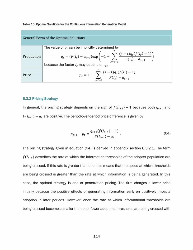
114

Table 15: Optimal Solutions for the Continuous Information Generation Model


Production

The value of can be implicitly determined by

( ( ) ) ( ∑( ) ( ( ) )

( )

)

because the factor may depend on

Price ∑( ) ( ( ) )

( )


In general, the pricing strategy depends on the sign of ( ) because both and

( ) are positive. The period-over-period price difference is given by

( ( ) )

( ) (64)

The pricing strategy given in equation (64) is derived in appendix section 6.3.2.1. The term

( ) describes the rate at which the information thresholds of the adopter population are

being crossed. If this rate is greater than one, this means that the speed at which thresholds

are being crossed is greater than the rate at which information is being generated. In this

case, the optimal strategy is one of penetration pricing. The firm charges a lower price

initially because the positive effects of generating information early on positively impacts

adoption in later periods. However, once the rate at which informational thresholds are

being crossed becomes smaller than one, fewer adopters’ thresholds are being crossed with

115

each new adoption. In this case, the firm begins to decrease the price, which means that a

skim pricing strategy becomes optimal.

6.3.2.1 Normally Distributed Information Requirements

If the information requirements are normally distributed, then the difference between prices

in successive periods is given as

√ ( (

( )

) √ )

( )

(65)

The pricing strategy for normally distributed information requirements and consequent

results are derived in appendix section A6.3.2.3. The sign of this expression depends on the

sign of (

( )

) √ If it is negative, the optimal pricing policy is a skimming

strategy. This corresponds to the following condition on the absolute difference between the

information and the mean of the distribution of information requirements: |( ) |

√ . The standard deviation is completely bounded by

√ . If the standard

deviation is greater than this value, then the firm always employs a skim pricing strategy,

regardless of the distribution mean, The absolute difference between the information

generated and the distribution mean is also bounded. If | |

√ , the firm’s optimal

strategy is for skim pricing regardless of the standard deviation of the distribution. When the

difference between the prices in two successive periods crosses the bound, this is the last

such difference that can be increasing period-by-period—the difference between the next

two successive prices must be negative.

116

Figure 39 provides an example of the boundary for the standard deviation and

various examples of for an eight-period planning problem. In the case of ( ), the

firm’s optimal strategy is to decrease the price it charges through all eight periods.

Meanwhile, the optimal strategy for a firm facing information needs of ( ) and

( ) is to increase prices in the early periods and decrease them until the end of the

planning horizon. As derived in the mathematical results, the pricing strategy in the green

region of Figure 39 is always one of price skimming.

Figure 39: Optimal Pricing Strategy for

The value of the sum ∑ is the information generated to date and the value of this term

continues to increase with adoption in each period. However, because the adoption cannot

exceed one, the total information in the system is also bounded. This means that it is

117

possible that the firm’s strategy can be one of penetration pricing over the whole planning

horizon.

6.3.3 Information Loss

In the previous analysis, all of the information in the system was assumed to be equally

good and to last for the entire planning horizon. When the information in the system,

∑ ( ) declines at a certain rate, the optimal solutions for price and

production are affected.

As illustrated in Figure 40, price, shown in panel (a), and per-period production, shown in

panel (b), have no consistent relationship with market adoption because the relationship

between the optimal solutions depends on the information rather than on the adoption rate.

Although they are very close, the terminal adoption rates for the systems where much

information is lost ( ) is higher than those where little information is lost ( ). The

numerical results depicted in Figure 40 and discussed in the remainder of this section are

given in appendix section A6.2.2.

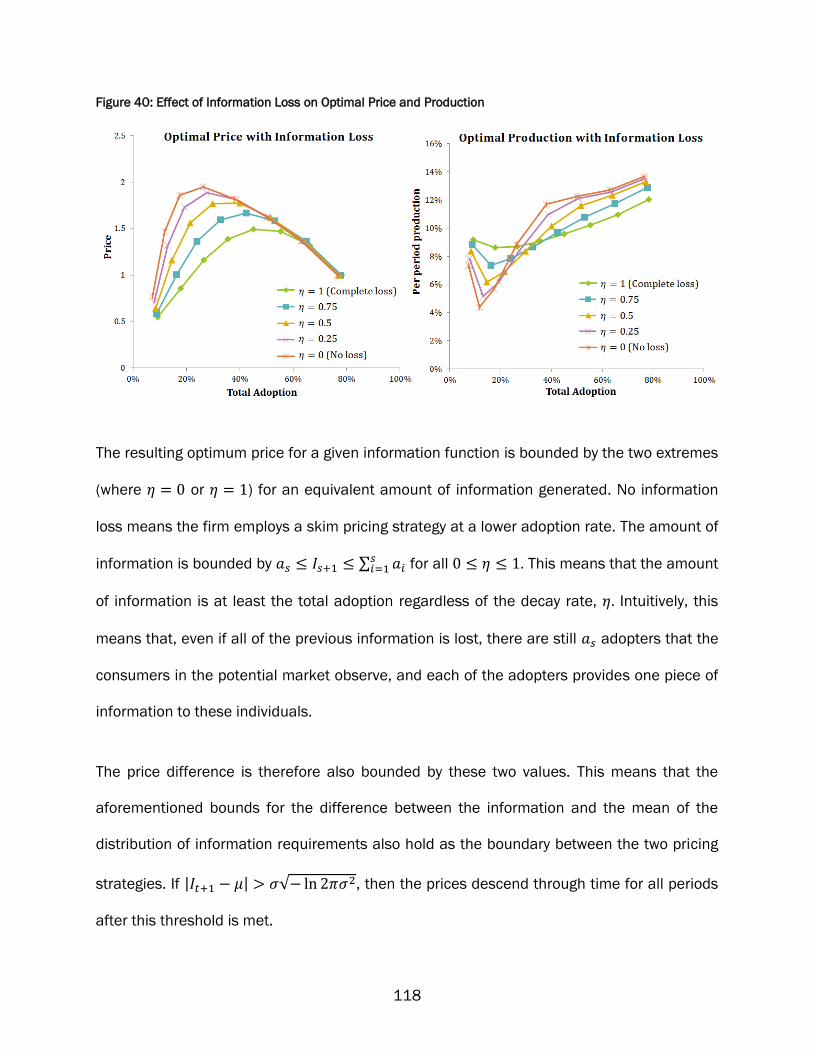
118

Figure 40: Effect of Information Loss on Optimal Price and Production

The resulting optimum price for a given information function is bounded by the two extremes

(where or ) for an equivalent amount of information generated. No information

loss means the firm employs a skim pricing strategy at a lower adoption rate. The amount of

information is bounded by ∑ for all This means that the amount

of information is at least the total adoption regardless of the decay rate, Intuitively, this

means that, even if all of the previous information is lost, there are still adopters that the

consumers in the potential market observe, and each of the adopters provides one piece of

information to these individuals.

The price difference is therefore also bounded by these two values. This means that the

aforementioned bounds for the difference between the information and the mean of the

distribution of information requirements also hold as the boundary between the two pricing

strategies. If | | √ , then the prices descend through time for all periods

after this threshold is met.

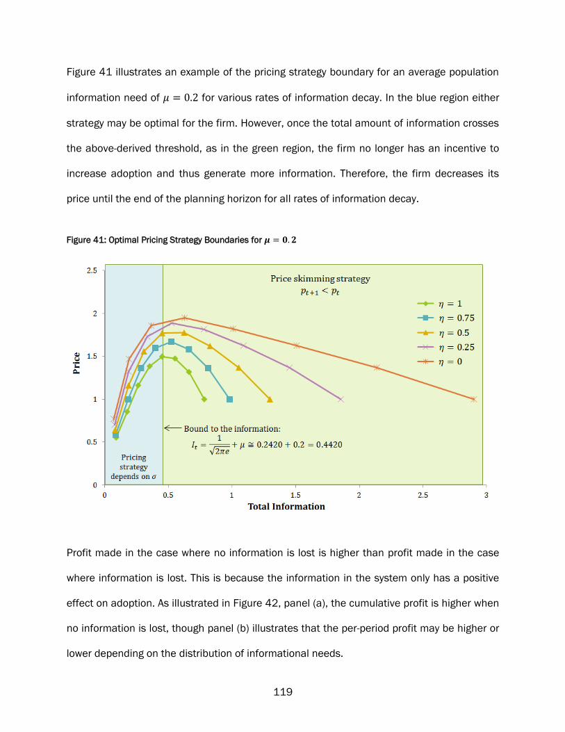
119

Figure 41 illustrates an example of the pricing strategy boundary for an average population

information need of for various rates of information decay. In the blue region either

strategy may be optimal for the firm. However, once the total amount of information crosses

the above-derived threshold, as in the green region, the firm no longer has an incentive to

increase adoption and thus generate more information. Therefore, the firm decreases its

price until the end of the planning horizon for all rates of information decay.

Figure 41: Optimal Pricing Strategy Boundaries for

Profit made in the case where no information is lost is higher than profit made in the case

where information is lost. This is because the information in the system only has a positive

effect on adoption. As illustrated in Figure 42, panel (a), the cumulative profit is higher when

no information is lost, though panel (b) illustrates that the per-period profit may be higher or

lower depending on the distribution of informational needs.

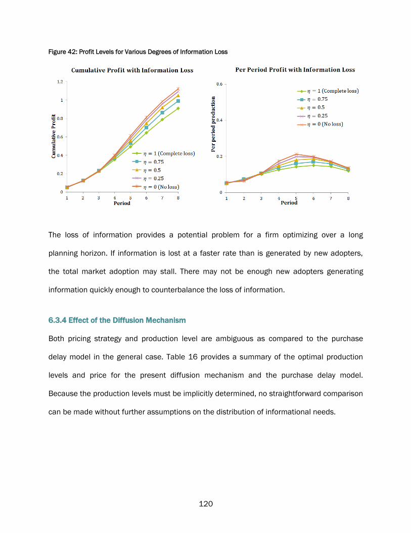
120

Figure 42: Profit Levels for Various Degrees of Information Loss

The loss of information provides a potential problem for a firm optimizing over a long

planning horizon. If information is lost at a faster rate than is generated by new adopters,

the total market adoption may stall. There may not be enough new adopters generating

information quickly enough to counterbalance the loss of information.


Both pricing strategy and production level are ambiguous as compared to the purchase

delay model in the general case. Table 16 provides a summary of the optimal production

levels and price for the present diffusion mechanism and the purchase delay model.

Because the production levels must be implicitly determined, no straightforward comparison

can be made without further assumptions on the distribution of informational needs.

121

Table 16: Effect of the Diffusion Mechanism on Optimal Production and Price


Diffusion by Information

( (∑

) ) ( ∑ ( )( (∑

))

(∑ )

)

—the value of is implicitly determined because the factor (∑ )

may depend on

Purchase Delay ( ) ( ∑

)

Optimal Price

Diffusion by Information

∑( ) ( ( ) )

( )

Purchase Delay ∑


Although a firm that can take into account the informational needs of the population and its

effect on diffusion can benefit in total profit, the optimal price and production may be higher

or lower as compared with the firm that only optimizes statically in each period. The effect of

foresight on optimal production and price depends on the distribution of information

requirements in the population. Table 17 provides a summary of the optimal production

levels and price for the statically optimized procedure and the fully optimal solution. The

static optimization solutions are derived in appendix section A6.3.3.

The difference between the statically optimized production and the fully optimal production

is ambiguous because of the interdependence of production on the information thresholds.

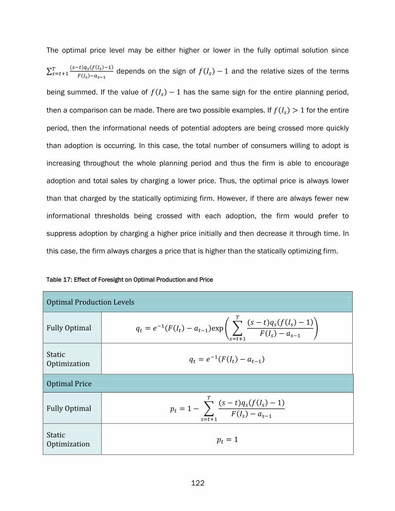
122

The optimal price level may be either higher or lower in the fully optimal solution since

∑( ) ( ( ) )

( )

depends on the sign of ( ) and the relative sizes of the terms

being summed. If the value of ( ) has the same sign for the entire planning period,

then a comparison can be made. There are two possible examples. If ( ) for the entire

period, then the informational needs of potential adopters are being crossed more quickly

than adoption is occurring. In this case, the total number of consumers willing to adopt is

increasing throughout the whole planning period and thus the firm is able to encourage

adoption and total sales by charging a lower price. Thus, the optimal price is always lower

than that charged by the statically optimizing firm. However, if there are always fewer new

informational thresholds being crossed with each adoption, the firm would prefer to

suppress adoption by charging a higher price initially and then decrease it through time. In

this case, the firm always charges a price that is higher than the statically optimizing firm.

Table 17: Effect of Foresight on Optimal Production and Price


Fully Optimal ( ( ) ) ( ∑( ) ( ( ) )

( )

)

Static Optimization

( ( ) )

Optimal Price

Fully Optimal ∑( ) ( ( ) )

( )

Static Optimization

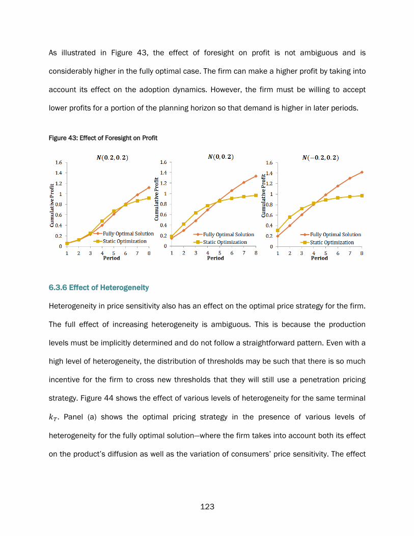
123

As illustrated in Figure 43, the effect of foresight on profit is not ambiguous and is

considerably higher in the fully optimal case. The firm can make a higher profit by taking into

account its effect on the adoption dynamics. However, the firm must be willing to accept

lower profits for a portion of the planning horizon so that demand is higher in later periods.



Heterogeneity in price sensitivity also has an effect on the optimal price strategy for the firm.

The full effect of increasing heterogeneity is ambiguous. This is because the production

levels must be implicitly determined and do not follow a straightforward pattern. Even with a

high level of heterogeneity, the distribution of thresholds may be such that there is so much

incentive for the firm to cross new thresholds that they will still use a penetration pricing

strategy. Figure 44 shows the effect of various levels of heterogeneity for the same terminal

Panel (a) shows the optimal pricing strategy in the presence of various levels of

heterogeneity for the fully optimal solution—where the firm takes into account both its effect

on the product’s diffusion as well as the variation of consumers’ price sensitivity. The effect

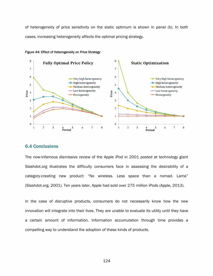
124

of heterogeneity of price sensitivity on the static optimum is shown in panel (b). In both

cases, increasing heterogeneity affects the optimal pricing strategy.

Figure 44: Effect of Heterogeneity on Price Strategy

6.4 Conclusions

The now-infamous dismissive review of the Apple iPod in 2001 posted at technology giant

Slashdot.org illustrates the difficulty consumers face in assessing the desirability of a

category-creating new product: “No wireless. Less space than a nomad. Lame”

(Slashdot.org, 2001). Ten years later, Apple had sold over 275 million iPods (Apple, 2013).

In the case of disruptive products, consumers do not necessarily know how the new

innovation will integrate into their lives. They are unable to evaluate its utility until they have

a certain amount of information. Information accumulation through time provides a

compelling way to understand the adoption of these kinds of products.

125

The analysis in Subsection 6.3 illustrates that if adopters generate information in each

period, it may be optimal to encourage adoption early on so that the information available to

new adopters increases more quickly and thus assists in diffusing the product. The general

model presented lends itself to many extensions by considering variability in the information

created and required.

The same three general forms of optimal pricing policies found in Chapters 4 and 5 are also

possible in this case:

Complete price skimming—a firm may use a decreasing price policy throughout the

planning horizon.

Complete penetration pricing—an increasing price policy throughout the planning

horizon may be optimal.

A combination of penetration pricing and price skimming—the optimal price policy

may take the form of an increasing price followed by a decreasing price.

The decay of information in the system is an important variable as it has a significant effect

on the firm’s profit levels. Since more information only has a positive effect on future

adoption in this model, more information affords a higher total profit to the firm. A firm that

could positively affect the retention of information in the system would then be able to

benefit. The model is deliberately abstract and so the specifics of how information is

understood and generated are simplified. However, the essential nature of this aspect could

benefit from empirical investigation to see if it could be affected by a firm.

126

Unlike the models discussed in Chapters 3 and 4, heterogeneity in price sensitivity does not

have a straightforward effect on the firm’s strategy. The positive effect of generating new

information by encouraging adoption may be stronger than the profit made by taking

advantage of the low price sensitivity in earlier periods. The heterogeneity due to

informational needs must be explicitly measured to fully resolve these effects.


1. On average, how much information does an individual need to consider adoption?

If a large amount of information is required for many consumers to purchase, it is more

likely to be optimal to utilize a skim pricing strategy to benefit from the initially low price

sensitivity among early adopters. This would be the case for a very innovative new product.

2. Do potential adopters vary considerably in their informational needs?

For a product that has a particular appeal to a specific group, there may be a wide variety of

informational needs. Products that are culturally or ethnically relevant are likely to elicit a

range of needs since some members of the adopter group will understand the use of the

product immediately while others will require much more information to adopt. If the

potential adopter population is diverse in the amount of information needed, it is more likely

that a skim pricing strategy will be optimal.

127

3. Is there any way to preserve or increase the amount of information available to

potential adopters?

Information provides a positive force to adoption in this model and allows the firm to

increase its profits. Therefore, a firm may benefit from encouraging the information

generation from adopters and non-adopters, perhaps through encouraging product use and

positive word-of-mouth. To fully understand whether a firm could affect the persistence of

information, more empirical research is needed.

128

REFERENCES

Allenby, Greg M., and Peter E. Rossi. 1998. “Marketing models of consumer heterogeneity,”

Journal of Econometrics, 89(1–2) 26: 57-78. doi:10.1016/S0304-4076(98)00055-4

Apple Corporation. 2013. “iPod History: iPod+ iTunes Timeline.” Accessed July 21, 2013.

http://www.apple.com/pr/products/ipodhistory/

Bagwell, Kyle, and Michael H. Riordan. 1991. “High and Declining Prices Signal Product

Quality,” American Economic Review, 81(1): 224–239.

Bass, Frank. 1969. “A New Product Growth Model for Consumer Durables,” Management

Science, 15(5): 215–227.

Bass, Frank M. 1980. “The Relationship Between Diffusion Rates, Experience Curves, and

Demand Elasticities for Consumer Durable Technological Innovations,” Journal of Business,

53(3): S51–S67.

Bass, Frank M., and Alain V. Bultez. 1982. “A Note on Optimal Strategic Pricing of Technical

Innovations,” Marketing Science,1(4): 371–378.

Bass, Frank M., Trichy V. Krishnan, and Dipak C. Jain. 1994. “Why the Bass Model Fits

without Decision Variables,” Marketing Science, 13(3): 203–223.

Bergemann, Dirk, and Juuso Välimäki. 1997. “Market Diffusion with Two-Sided Learning,”

RAND Journal of Economics, 28(4): 773–795.

Bergstein, Heather, and Hooman Estelami. 2002. “A survey of emerging technologies for

pricing new-to-the-world products,” Journal of Product & Brand Management, 11(5): 303–

319.

129

Bikhchandani, Sushil, David Hirshleifer, and Ivo Welch. 1992. “A Theory of Fads, Fashion,

Custom, and Cultural Change as Informational Cascades,” Journal of Political Economy,

100(5): 992–1026.

Blinder, Alan S. 1991. “Why are Prices Sticky? Preliminary Results from an Interview Study,”

American Economic Review, 81(2): 89–96.

Chao, C.-W., M. Reid, and F. T. Mavondo. 2012. “Consumer innovativeness influence on

really new product adoption,” Australasian Marketing Journal, 20(3): 211–217.

Chatterjee, Rabik A., and Jehoshua Eliashberg. 1990. “The Innovation Diffusion Process in a

Heterogeneous Population: A Micromodeling Approach,” Management Science, 36(9):

1057–1079.

Choi, Hanool, Sang-Hoon Kim, and Jeho Lee. 2010. “Role of network structure and network

effects in diffusion of innovations” Industrial Marketing Management, 39(1) 170–177.

Ding, Min, William T. Ross Jr., and Vithala R. Rao. 2010. “Price as an Indicator of Quality:

Implications for Utility and Demand Functions,” Journal of Retailing, 86(1): 69–84.

Dolan, Robert J., and Abel P. Jeuland. 1981 “Experience Curves and Dynamic Demand

Models: Implications for Optimal Pricing Strategies,” Journal of Marketing, 45(1): 52–62,

Eliashberg, Jehoshua, and Rabikar Chatterjee. 1985. “Analytical Models of Competition with

Implications for Marketing: Issues, Findings, and Outlook,” Journal of Marketing Research,

22(3): 237–261.

Eliashberg, Jehoshua and Abel P. Jeuland. 1986. “The Impact of Competitive Entry in a

Developing Market upon Dynamic Pricing Strategies,” Marketing Science, 5(1): 20–36.

Ellison, Glenn, and Drew Fudenberg. 1995. “Word-of-Mouth Communication and Social

Learning,” The Quarterly Journal of Economics, 110(1): 93–125.

130

Farias, Vivek F., and Benjamin Van Roy. 2010. “Dynamic Pricing with a Prior on Market

Response,” Operations Research, 58:16–29.

Forker, Olan, and Ronald W. Ward. 1993. Commodity Advertising: The Economics and

Measurement of Generic Programs. New York: Lexington Books.

Gourville, John T. 2006. “Eager Sellers and Stony Buyers: Understanding the Psychology of

New-Product Adoption,” Harvard Business Review, June 2006.

Gourville, John, and Dilip Soman. 2002. “Pricing and the Psychology of Consumption,”

Harvard Business Review, September.

Granovetter, Mark. 1978. “Threshold Models of Collective Behavior,” American Journal of

Sociology, 83(6): 1420–1443.

Hall, Simon, Mark Walsh, and Anthony Yates. 1996. “How do UK companies set prices?”

Bank of England Working Paper #67.

Henrich, Joseph. 2001. “Cultural Transmission and the Diffusion of Innovations: Adoption

Dynamics Indicate That Biased Cultural Transmission Is the Predominate Force in Behavioral

Change,” American Anthropologist, New Series, 103(4): 992–1013.

Hohnisch, Martin, Sabine Pittnauer, and Dietrich Stauffer. 2008. “A percolation-based model

explaining delayed takeoff in new-product diffusion,” Industrial and Corporate Change,

17(5): 1001–1017. doi:10.1093/icc/dtn031

Horsky, Dan. 1990. “A Diffusion Model Incorporating Product Benefits, Price, Income and

Information,” Marketing Science, 9(4): 342–365.

Jedidi, Kamel, and Z. John Zhang. 2002. “Augmenting Conjoint Analysis to Estimate

Consumer Reservation Price,” Management Science, 48(10): 1350–1368.

131

Jovanovic, Boyan, and Glenn M. MacDonald. 1994. “The Life Cycle of a Competitive

Industry,” Journal of Political Economy, 102(2): 322–347.

Kalish, Shlomo. 1983. “Monopolist Pricing with Dynamic Demand and Production Cost,”

Marketing Science, 2(2): 135–159. doi: 10.1287/mksc.2.2.135

Kalish, Shlomo. 1985. “A New Product Adoption Model with Price, Advertising, and

Uncertainty.” Management Science, 31(12): 1569–1585.

Katz, Michael L., and Carl Shapiro. 1985. “Network Externalities, Competition, and

Compatibility,” American Economic Review, 75(3): 424–440.

Katz, Michael L., and Carl Shapiro. 1994. ”Systems competition and network effects.”

Journal of Economic Perspectives, 8(2): 93–115.

Kohli, Rajeev, and Vijay Mahajan. 1991. “A reservation-price model for optimal pricing of

multiattribute products in conjoint analysis,” Journal of Marketing Research, 28(3): 347–

354.

Krishnan, Trichy V., Frank M. Bass, and Dipak C. Jain. 1999. “Optimal Pricing Strategy for

New Products,” Management Science, 45(12): 1650–1663.

Lamberson, P. J. 2010. “Social Learning in Social Networks.” B.E. Journal of Theoretical

Economics, 10(1): 1–31.

Lavidge, Robert J., and Gary A. Steiner. 1961. “A Model for Predictive Measurements of

Advertising Effectiveness,” Journal of Marketing, 25(6): 59–62.

Lekvall, Per, and Clas Wahlbin. 1973. “A Study of Some Assumptions Underlying Innovation

Diffusion Functions,” Swedish Journal of Economics, 75(4): 362–377.

Mahajan, Vijay, and Robert A. Peterson. 1978. “Innovation Diffusion in a Dynamic Potential

Adopter Population,” Management Science, 24(15): 1589–1597.

132

Metcalfe, J. Stanley. 1998. Evolutionary Economics and Creative Destruction. Routledge

Chapman & Hall.

Monroe, Kent B., and Albert J. Della Bitta. 1978. “Models for Pricing Decisions,” Journal of

Marketing Research, 15(3): 413–428.

Navarro, Noemí. 2012. “Price and quality decisions under network effects,” Journal of

Mathematical Economics, 48(5): 263–270.

Nelson, Richard R., Alexander Peterhansl, and Bhaven Sampat. 2004. “Why and how

innovations get adopted: a tale of four models,” Industrial and Corporate Change, 13(5):

679–699. doi: 10.1093/icc/dth027

Nevo, Aviv. 2011. “Empirical Models of Consumer Behavior,” Annual Review of Economics,

Annual Reviews, 3(1): 51–75.

Parker, Philip M. 1992. “Price Elasticity Dynamics over the Adoption Life Cycle,” Journal of

Marketing Research, 29(3): 358–367.

Peres, Renana, Eitan Muller, and Vijay Mahajan. 2010. “Innovation diffusion and new

product growth models: A critical review and research directions,” International Journal of

Research in Marketing, 27(2): 91–106. doi:10.1016/j.ijresmar.2009.12.012

Rao, Ram C., and Frank M. Bass. 1985. “Competition, Strategy, and Price Dynamics: A

Theoretical and Empirical Investigation,” Journal of Marketing Research, 22(3): 283–296.

Robinson, Bruce, and Chet Lakhani. 1975. “Dynamic Price Models for New-Product

Planning,” Management Science, 21(10): 1113–1122.

Rogers, Everett. 1983. Diffusion of Innovations (Third Edition). New York, NY: Free Press.

133

Roll, Oliver, Lars-Hendrik Achterberg, and Karl-Georg Herbert. 2010. “Innovative approaches

to analyzing the Price Sensitivity Meter: Results of an international comparative study,”

Combi2010 Conference Proceedings, October.

Ryan, Bryce, and Neal C. Gross. 1943. “The Diffusion of Hybrid Corn in Two Iowa

Communities,” Rural Sociology, 8(1): 15–24.

Schelling, Thomas C. 1971. “Dynamic Models of Segregation,” Journal of Mathematical

Sociology, 1: 143–86.

Schelling, Thomas C. 1978. Micromotives and Macrobehavior. New York: Norton.

Slashdot.org. 2001. “Apple Releases iPod.” Accessed July 21, 2013.

http://slashdot.org/story/01/10/23/1816257/apple-releases-ipod

Tellis, Gerard J. 1988. “The Price Elasticity of Selective Demand: A Meta-Analysis of

Econometric Models of Sales,” Journal of Marketing Research, 25(4): 331–341.

Teng, Jinn-Tsair, Gerald Luther Thompson, and Carnegie Mellon University Design Research

Center. 1984. “Optimal strategies for general price-advertising models,” Tepper School of

Business. Paper 956. http://repository.cmu.edu/tepper/956

Thompson, Gerald L., and Jinn-Tsair Teng. 1984. “Optimal Pricing and Advertising Policies

for New Product Oligopoly Models,” Marketing Science, 3(2): 148–168.

Van Westendorp, P. E. 1976. “NSS price sensitivity meter – a new approach to study

consumer perceptions of price,” ESOMAR Venice Congress Proceedings, 140–66.

Vettas, Nikolaos. 1998. “Demand and Supply in New Markets: Diffusion with Bilateral

Learning,” RAND Journal of Economics, 29(1): 215–233.

Young, Peyton H. 2009. “Innovation Diffusion in Heterogeneous Populations: Contagion,

Social Influence, and Social Learning.” American Economic Review, 99(5): 1899–1924.

134

APPENDICES

A3 Appendix to Chapter 3

A3.1 The Two-Period Case

A3.1.1 Derivation of the Two Period Full Optimization

The firm’s two-period problem is described by

{

( )

(

)}

which gives the first-order conditions

( )

and

(

)

Therefore,

(

)

⇔

⇔ ( )

and so production for both periods can be derived to be

( )

⇔ ( )

⇔

135

and

( ) (

)

Price in each period is

( )

(

)

(

)

and

(

)

(

)

A3.1.2 Derivation of the Pricing Strategy

The difference in prices between periods one and two is

(

)

Since

which means that (

) . Therefore . A skim

pricing strategy is always optimal.

A3.1.3 Derivation of the Two Period Static Optimization

In the case of static optimization, the firm solves the two-period problem separately. In

period 1, the firm’s maximization problem is

{

( ) }

136

which has the first-order condition

( )

Therefore production in the first period is

( )

⇔ ( )

⇔

This gives the first-period price

( )

In period 2, the firm solves the following problem using the first-period solution

{

(

) }

⇔

{

(

) }

The first-order condition is

(

)

which allows the explicit solution for to be derived as

(

)

⇔

⇔ ( )

137

Therefore the price in the second period is

(

)

(

( )

)

A3.2 The Eight-Period Case

The maximization problem over eight periods is

{

( )

(

)

(

)

(

)

(

)

(

)

(

)

(

)}

The first-order conditions are:

( )

( )

( )

( )

( )

( )

( )

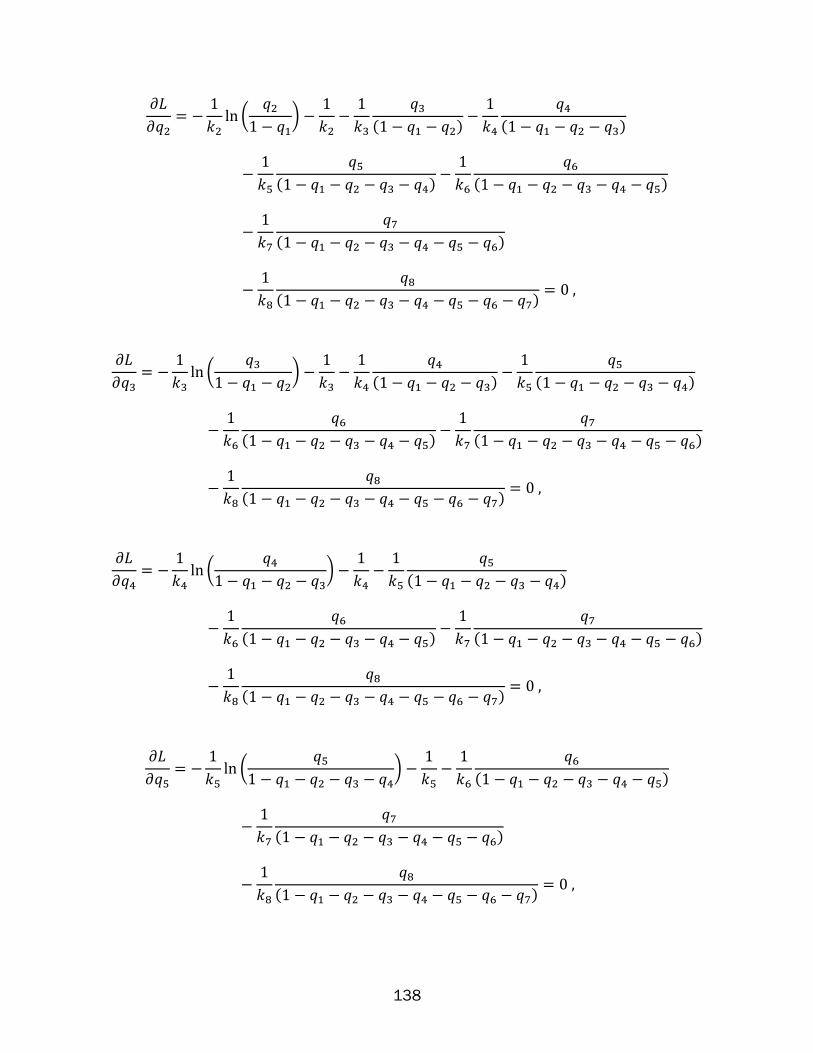
138

(

)

( )

( )

( )

( )

( )

( )

(

)

( )

( )

( )

( )

( )

(

)

( )

( )

( )

( )

(

)

( )

( )

( )

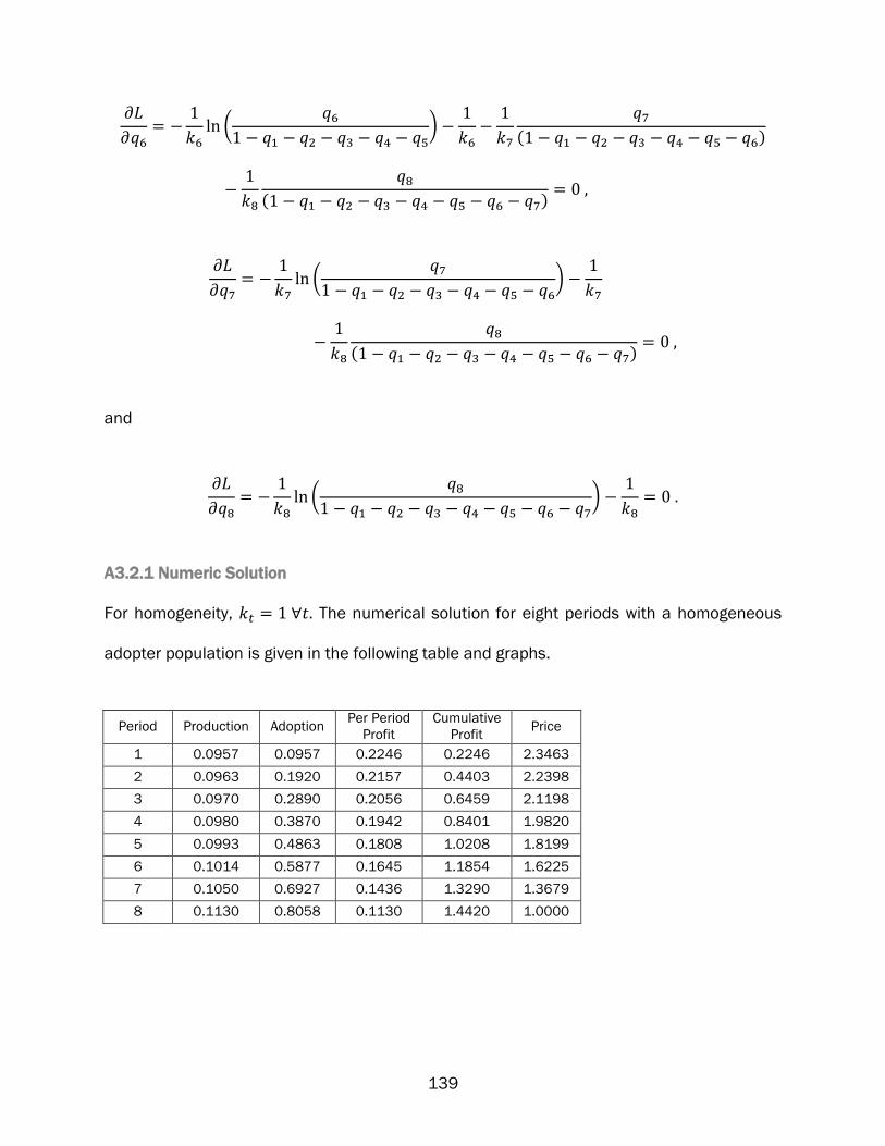
139

(

)

( )

( )

(

)

( )

and

(

)

A3.2.1 Numeric Solution

For homogeneity, The numerical solution for eight periods with a homogeneous

adopter population is given in the following table and graphs.

Period Production Adoption Per Period

Profit

Cumulative

Profit Price

1 0.0957 0.0957 0.2246 0.2246 2.3463

2 0.0963 0.1920 0.2157 0.4403 2.2398

3 0.0970 0.2890 0.2056 0.6459 2.1198

4 0.0980 0.3870 0.1942 0.8401 1.9820

5 0.0993 0.4863 0.1808 1.0208 1.8199

6 0.1014 0.5877 0.1645 1.1854 1.6225

7 0.1050 0.6927 0.1436 1.3290 1.3679

8 0.1130 0.8058 0.1130 1.4420 1.0000

140

A3.3 The T-Period Case

A3.3.1 Derivation of Optimal Production and Price over T Periods

Suppose the firm wants to maximize their profit by choosing a single price that will maximize

their profit over a T-period planning horizon. Therefore the firm maximizes

{∑

(

( ∑

)

)

}

This maximization problem yields a set of first-order conditions

(

∑

)

∑

( ∑ )

Therefore production in period is given by

(

∑

)

∑

( ∑ )

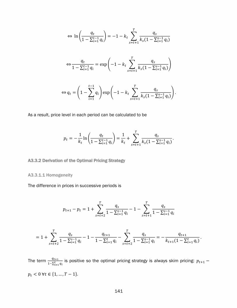
141

⇔ (

∑

) ∑

( ∑ )

⇔

∑

( ∑

( ∑ )

)

⇔ ( ∑

) ( ∑

( ∑ )

)

As a result, price level in each period can be calculated to be

(

∑

)

∑

( ∑ )

A3.3.2 Derivation of the Optimal Pricing Strategy

A3.3.1.1 Homogeneity

The difference in prices in successive periods is

∑

∑

∑

∑

∑

∑

∑

∑

∑

( ∑ )

The term

∑

is positive so the optimal pricing strategy is always skim pricing:

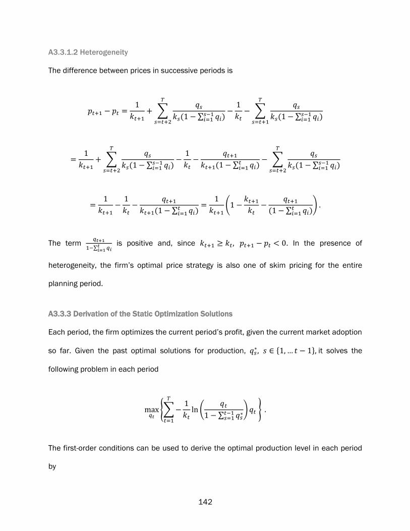
142

A3.3.1.2 Heterogeneity

The difference between prices in successive periods is

∑

( ∑ )

∑

( ∑ )

∑

( ∑ )

( ∑ )

∑

( ∑ )

( ∑ )

(

( ∑ )

)

The term

∑

is positive and, since . In the presence of

heterogeneity, the firm’s optimal price strategy is also one of skim pricing for the entire

planning period.

A3.3.3 Derivation of the Static Optimization Solutions

Each period, the firm optimizes the current period’s profit, given the current market adoption

so far. Given the past optimal solutions for production, it solves the

following problem in each period

{∑

(

∑

)

}

The first-order conditions can be used to derive the optimal production level in each period

by

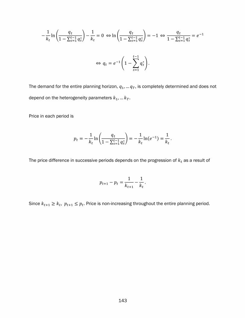
143

(

∑

)

⇔ (

∑

)

⇔

∑

⇔ ( ∑

)

The demand for the entire planning horizon, , is completely determined and does not

depend on the heterogeneity parameters .


(

∑

)

( )

The price difference in successive periods depends on the progression of as a result of

Since . Price is non-increasing throughout the entire planning period.

144



A4.1.1 Derivation of the Two Period Full Optimization

The firm maximizes their profit over two periods by solving the following problem

{

(

)

(

( )( ))}

⇔

{

(

)

(

( )( )) }


In the homogeneity case, the firm solves the following maximization problem:

{ (

) (

( )( )) }

which yields the first-order conditions

(

) (

( )( )

( ) ( )

( )( )

( )( ) )

and

(

( )( ))

Therefore,

145

(

) (

)

⇔ (

)

( )( ) ( )

⇔

( )( ) (

(

)

)

Using the latter first-order condition,

(

( )( ))

⇔

( )( )

Combining them we can derive the relation for period 1 production:

( (

)

)

⇔ (

) ( )

⇔ (

)

⇔

(

)

⇔ (

) (

)

The value of can be expressed by using the main branch of the Lambert W function,

( ) which is defined by ( ) ( ) and is not expressible by elementary functions.

146

Using the identity ( ) ⇒

( )

we can obtain closed-form expression for

( (

))

( )

where (

) which depends only on the coefficients of the diffusion

mechanism, and

This allows us to also derive the closed form expression for to be

( )( )

( (

( )) )( (

( )))

(

( )

)(

( ))

Price in the first period can be derived using the identity ( ( )) ( ) ( ):

(

) (

( )) (

) ( )

(

(

)) ( (

))

( (

)) ( (

))

147

( (

))

The second period price is simply found using the first-order conditions to be

(

( )( ))


The firm solves the following maximization problem in the heterogeneous case:

{

(

)

(

( )( )) }

The two first-order conditions are

(

)

( ( )( )

( ) ( )

( )( )

( )( ) )

and

(

( )( ))

Therefore, using the former first-order condition,

(

)

(

)

⇔

(

)

(

)

148

⇔

(

)

(

)

⇔

(

)

(

( )

( )( )

( )

( )( ))

⇔

(

)

( ( ( ) ( ))

( )( ))

⇔

(

)

( ( )

( )( ))

⇔ (

)

( )( ) ( )

⇔

( )( )

( ( )

)

The latter first-order condition can then be used to derive

(

( )( ))

⇔

( )( )

Therefore, combining these two gives

(

(

)

)

⇔ (

)

( )

⇔ (

)

( )

⇔

(

( ) )

149

⇔ (

) (

)

The value of can be expressed by using the main branch of the Lambert W function,

( ) which is defined by ( ) ( ). Using the identity: ( ) ⇒

( )

( (

)

)

(

( ) (

))

(

(

))

( )

where

(

)

Likewise, a closed form expression for can be derived to be

( )( )

(

( ) ) (

( ))

The price in the first period is

(

)

(

( ))

Using the identity ( ( )) ( ) ( )

(

)

( )

(

(

))

( )

150

( ( ) (

))

( )

(

)

( )

( )

(

( ))

The second period price can be directly derived by the latter first order condition to be

(

( )( ))



The difference between price in periods 1 and 2 is

( (

))

( (

))

When the parameters are equal, the second period price is lower than the first period price—

the strategy is for skim pricing. This is because the value of (

) must be

positive since , , and ( ) Since ( ) , the right-hand

side is negative. Therefore .

Since ⇒ the region is bounded. The bound of the pricing

strategy is given by the condition that Therefore,

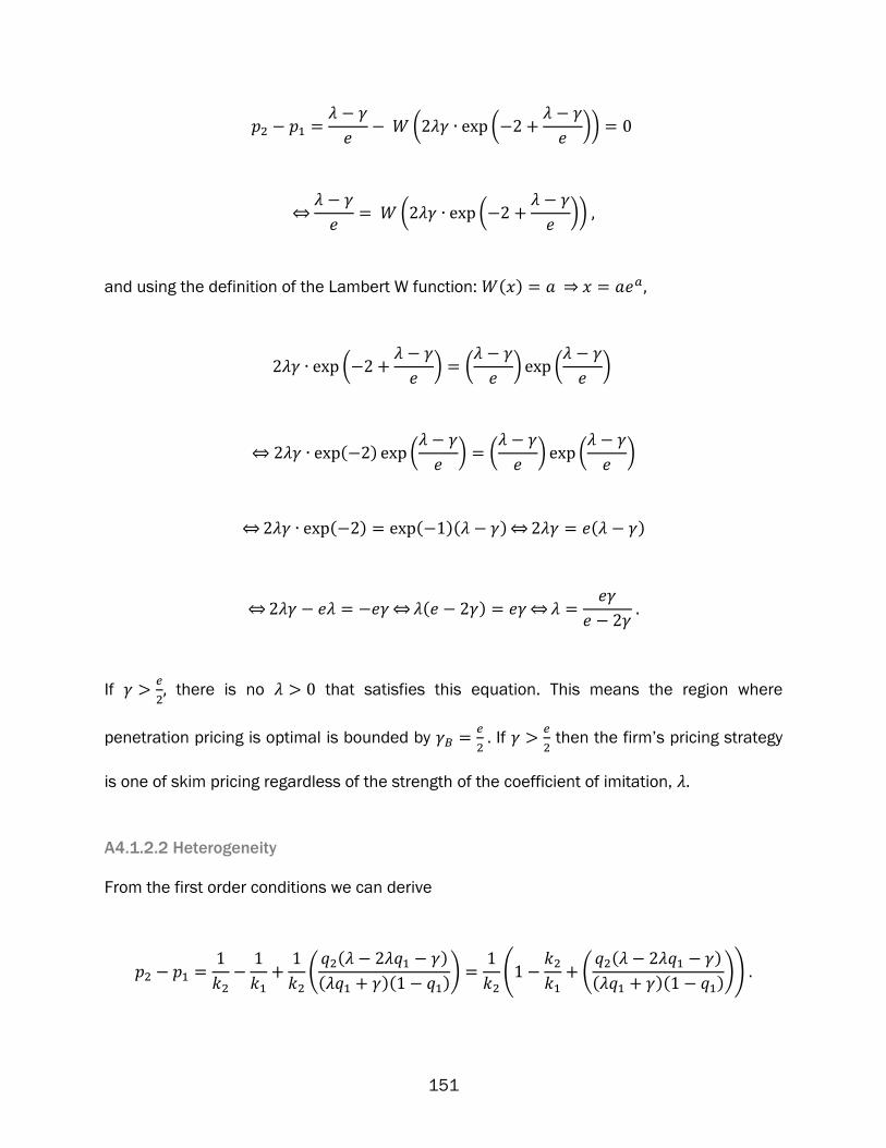
151

( (

))

⇔

( (

))

and using the definition of the Lambert W function: ( ) ⇒

(

) (

) (

)

⇔ ( ) (

) (

) (

)

⇔ ( ) ( )( )

⇔ ( )

⇔

⇔ ( )

⇔

If

there is no that satisfies this equation. This means the region where

penetration pricing is optimal is bounded by

If

then the firm’s pricing strategy

is one of skim pricing regardless of the strength of the coefficient of imitation,


From the first order conditions we can derive

( ( )

( )( ))

(

(

( )

( )( )))

152

Since

( )( )

,

(

(

( )

))

(

(

( )

) (

))

We have

( ) where

(

), which means that

(

(

) (

( ) ))

(

( )

( ))

Heterogeneity can always cause the firm’s optimal strategy to shift to one of skim pricing,

regardless of the strength of the coefficient of imitation, Formally,

.

The boundary of the region is given by

(

(

))

⇔

(

(

))

⇔ (

(

))

Using the definition of the Lambert W function, ( ) ⇒ ,

153

(

) (

) (

)

⇔

(

) ( )

(

) (

) (

)

⇔

(

) (

)

⇔

(

) (

) (

)

⇔ (

) (

)

(

)

(

) (

)

( (

))

⇔

(

) (

) (

)

(

)

(

) (

)

(

)

⇔

(

) (

)

(

)

(

) (

) (

)

(

)

⇔

(

) (

) (

)

(

)

(

) (

) (

)

(

)

154

Since

the numerator is always positive. Therefore the sign depends on the

denominator. Seeing as

, (

) . This means that, regardless of the amount of

heterogeneity, if

there is no that satisfies this equation. This is the ultimate

bound for which is exactly the one derived in under homogeneity. Given any amount of

heterogeneity and coefficient of innovation, the coefficient of imitation cannot necessarily be

increased to the point where a penetration pricing strategy is optimal because the region

where the penetration pricing strategy is optimal is bounded. If equals or exceeds the

boundary derived above, no amount of heterogeneity can cause the optimal pricing strategy

to be one of penetration pricing. Formally, ⇒

For a known degree of heterogeneity, there is a closer bound on If (

)

, then there is

no positive which satisfies this equation. This means that increasing beyond this limit

can always alter the firm’s optimal strategy from one of penetration pricing to one of skim

pricing, but that increasing the coefficient of imitation, , cannot necessarily change the

firm’s optimal strategy back to one of penetration pricing. Note that the curvature effect in

the numerator does not change the asymptotic bound of but that an increasing

has an

ambiguous effect on depending on the values of

and

The results above are due to the dynamics describing the number of new willing adopters in

the second period. When the coefficient of innovation is high enough, the firm has no need

to spur adoption by charging a low price in the first period. Instead, it can do better by taking

155

advantage of the relatively low price sensitivity, which is caused by the increased ratio

,

thus making a price skimming strategy optimal.

However, if both parameters and are free to take any value, then for any amount of

heterogeneity a parameter pair can be found such that penetration pricing is optimal.

Formally,

This is because the boundary of is positive in

its limit:

(

)

In the case where there is a relatively strong

effect of imitation and a relatively weak ( ) effect of innovation, the firm may need to

use a penetration pricing strategy despite the increasingly high price sensitivity in order to

have any demand at all in the second period.

A4.1.3 Two-Period Static Optimization

Two-period static optimization yields the first period problem

{

(

) }

which gives the first-order condition

(

)

Since there is no diffusion, the first period production does not depend on the parameters of

diffusion, nor on the parameter of heterogeneity, . Therefore the production level can be

solved for completely as

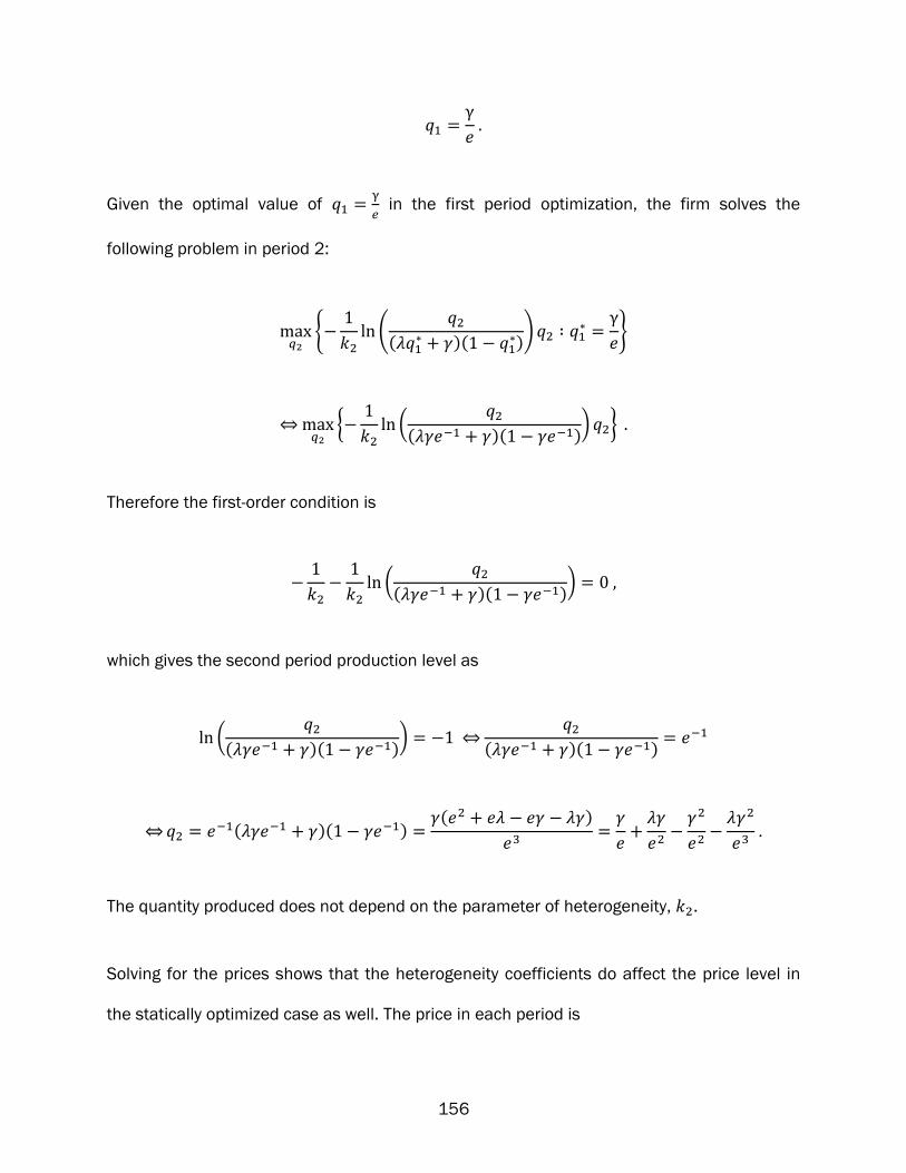
156

Given the optimal value of

in the first period optimization, the firm solves the

following problem in period 2:

{

(

( )(

))

}

⇔

{

(

( )( )) }

Therefore the first-order condition is

(

( )( ))

which gives the second period production level as

(

( )( ))

⇔

( )( )

⇔ ( )( )

( )

The quantity produced does not depend on the parameter of heterogeneity, .

Solving for the prices shows that the heterogeneity coefficients do affect the price level in

the statically optimized case as well. The price in each period is

157

(

)

(

)

and

(

( )( ))

The price is constant across periods if the population is homogenous. In the case where

. This means that any amount of heterogeneity induces a price path that

decreases through time.


The maximization problem over eight periods is

{

(

)

(

( )( ))

(

( )( ))

(

( )( ))

(

( )( ))

(

( )( ))

(

( )( ))

(

( )( ))}

The first-order conditions are:

158

(

)

( ) ( )

( )( )

( ) ( )

( )( )

( ) ( )

( )( )

( ) ( )

( )( )

( ) ( )

( )( )

( ) ( )

( )( )

( ) ( )

( )( )

(

( )( ))

( ) ( )

( )( )

( ) ( )

( )( )

( ) ( )

( )( )

( ) ( )

( )( )

( ) ( )

( )( )

( ) ( )

( )( )

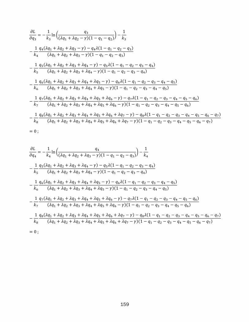
159

(

( )( ))

( ) ( )

( )( )

( ) ( )

( )( )

( ) ( )

( )( )

( ) ( )

( )( )

( ) ( )

( )( )

(

( )( ))

( ) ( )

( )( )

( ) ( )

( )( )

( ) ( )

( )( )

( ) ( )

( )( )

160

(

( )( ))

( ) ( )

( )( )

( ) ( )

( )( )

( ) ( )

( )( )

(

( )( ))

( ) ( )

( )( )

( ) ( )

( )( )

(

( )( ))

( ) ( )

( )( )

(

( )( ))

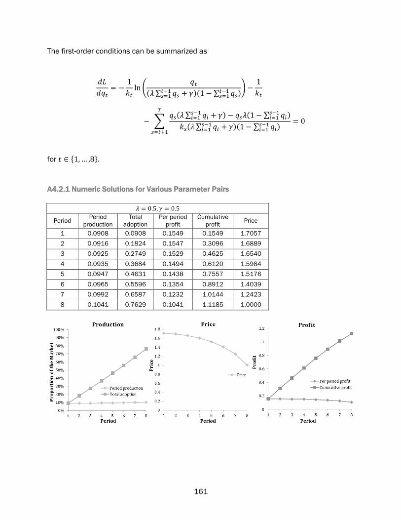
161

The first-order conditions can be summarized as

(

( ∑

)( ∑

)

)

∑ ( ∑

) ( ∑

)

( ∑ )( ∑

)

for

A4.2.1 Numeric Solutions for Various Parameter Pairs

Period Period

production

Total

adoption

Per period

profit

Cumulative

profit Price

1 0.0908 0.0908 0.1549 0.1549 1.7057

2 0.0916 0.1824 0.1547 0.3096 1.6889

3 0.0925 0.2749 0.1529 0.4625 1.6540

4 0.0935 0.3684 0.1494 0.6120 1.5984

5 0.0947 0.4631 0.1438 0.7557 1.5176

6 0.0965 0.5596 0.1354 0.8912 1.4039

7 0.0992 0.6587 0.1232 1.0144 1.2423

8 0.1041 0.7629 0.1041 1.1185 1.0000

162

Period Production Adoption Per Period

Profit

Cumulative

Profit Price

1 0.0720 0.0720 0.0236 0.0236 0.3283

2 0.0782 0.1502 0.0525 0.0761 0.6710

3 0.0822 0.2324 0.0730 0.1491 0.8887

4 0.0851 0.3175 0.0873 0.2364 1.0256

5 0.0875 0.4050 0.0964 0.3328 1.1016

6 0.0898 0.4947 0.1009 0.4337 1.1247

7 0.0922 0.5869 0.1009 0.5347 1.0944

8 0.0955 0.6824 0.0955 0.6301 1.0000

Period Period

production

Total

adoption

Per Period

Profit

Cumulative

Profit Price

1 0.0460 0.0460 0.0038 0.0038 0.0824

2 0.0484 0.0945 0.0176 0.0214 0.3633

3 0.0500 0.1445 0.0283 0.0497 0.5653

4 0.0512 0.1957 0.0366 0.0863 0.7148

5 0.0521 0.2478 0.0430 0.1293 0.8261

6 0.0528 0.3005 0.0479 0.1772 0.9077

7 0.0534 0.3539 0.0515 0.2287 0.9647

8 0.0539 0.4079 0.0539 0.2826 1.0000

163

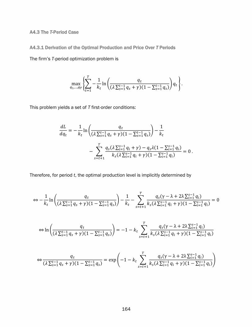
164


A4.3.1 Derivation of the Optimal Production and Price Over T Periods

The firm’s T-period optimization problem is

{∑

(

( ∑

)( ∑

)

)

}

This problem yields a set of T first-order conditions:

(

( ∑

)( ∑

)

)

∑ ( ∑

) ( ∑

)

( ∑ )( ∑

)

Therefore, for period t, the optimal production level is implicitly determined by

⇔

(

( ∑

)( ∑

)

)

∑

( ∑ )

( ∑ )( ∑

)

⇔ (

( ∑

)( ∑

)

) ∑ ( ∑

)

( ∑ )( ∑

)

⇔

( ∑

)( ∑

)

( ∑ ( ∑

)

( ∑ )( ∑

)

)

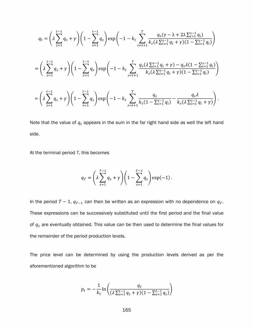
165

( ∑

)( ∑

) ( ∑ ( ∑

)

( ∑ )( ∑

)

)

( ∑

)( ∑

) ( ∑ ( ∑

) ( ∑

)

( ∑ )( ∑

)

)

( ∑

)( ∑

) ( ∑

( ∑ )

( ∑ )

)

Note that the value of appears in the sum in the far right hand side as well the left hand

side.

At the terminal period T, this becomes

( ∑

)( ∑

) ( )

In the period , can then be written as an expression with no dependence on .

These expressions can be successively substituted until the first period and the final value

of are eventually obtained. This value can be then used to determine the final values for

the remainder of the period production levels.

The price level can be determined by using the production levels derived as per the

aforementioned algorithm to be

(

( ∑

)( ∑

)

)

166

∑

( ∑ ) ( ∑

)

( ∑ )( ∑

)

∑

( ∑ )

( ∑ )

The price level depends both on the past and future production levels.



Under homogeneity, the price difference in successive periods is

∑ ( ∑

) ( ∑

)

( ∑ )( ∑

)

∑ ( ∑

) ( ∑

)

( ∑ )( ∑

)

( ∑

) ( ∑

)

( ∑ )( ∑

)

∑ ( ∑

) ( ∑

)

( ∑ )( ∑

)

∑ ( ∑

) ( ∑

)

( ∑ )( ∑

)

( ∑

) ( ∑

)

( ∑ )( ∑

)

( ∑

)

( ∑ )( ∑

)

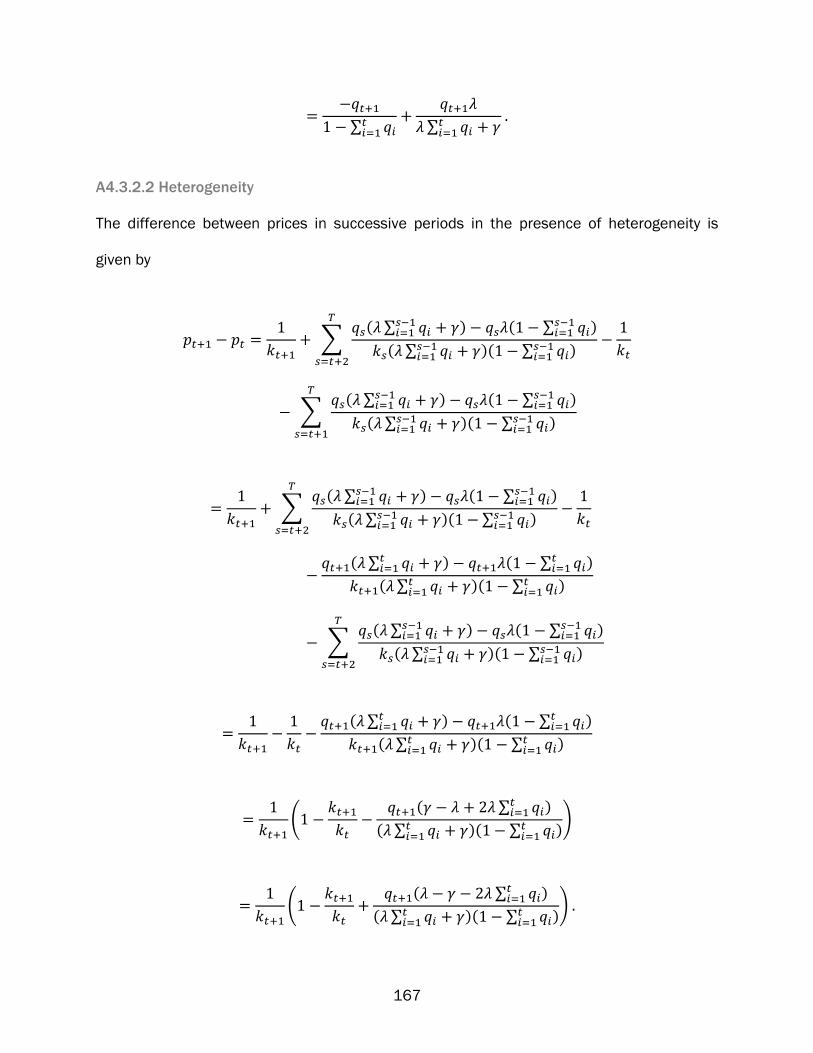
167

∑

∑


The difference between prices in successive periods in the presence of heterogeneity is

given by

∑

( ∑ ) ( ∑

)

( ∑ )( ∑

)

∑ ( ∑

) ( ∑

)

( ∑ )( ∑

)

∑

( ∑ ) ( ∑

)

( ∑ )( ∑

)

( ∑

) ( ∑

)

( ∑ )( ∑

)

∑ ( ∑

) ( ∑

)

( ∑ )( ∑

)

( ∑ ) ( ∑

)

( ∑ )( ∑

)

(

( ∑ )

( ∑ )( ∑

)

)

(

( ∑ )

( ∑ )( ∑

)

)

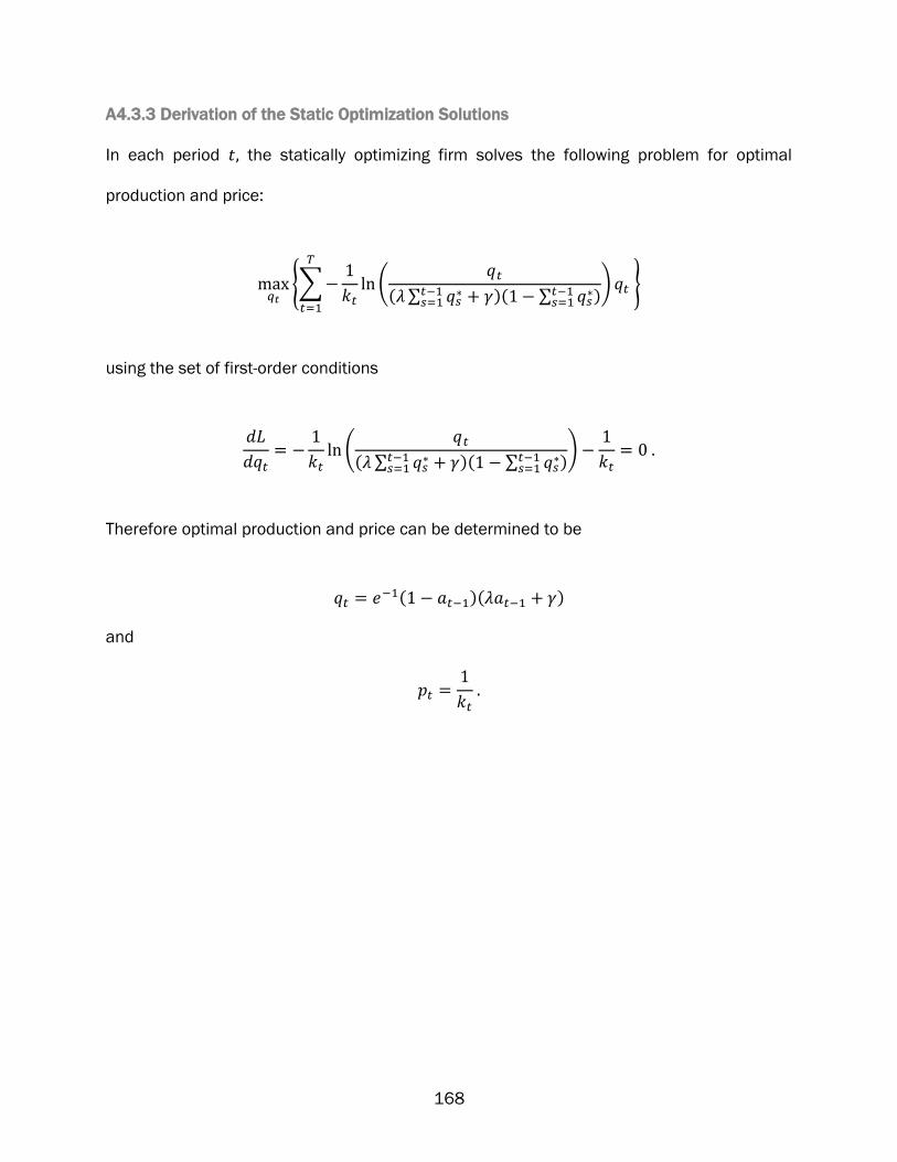
168


In each period the statically optimizing firm solves the following problem for optimal

production and price:

{∑

(

( ∑

)( ∑

)

)

}

using the set of first-order conditions

(

( ∑

)( ∑

)

)

Therefore optimal production and price can be determined to be

( )( )

and

169



A5.1.1 Derivation of the Two-Period Full Optimization

In the two-period full optimization, the firm solves the following maximization problem:

{ (

( )) (

( ) ) }

The first-order conditions are

(

( ))

( )

( ( ) )

and

(

( ) )

Therefore production in period 2 is

(

( ) )

⇔

( )

⇔ ( ( ) )

Combining this with the former first order condition yields the implicit expression for :

(

( )) ( ( ) )

which can be determined knowing the distribution of thresholds in the population, ( )

170

The price in the first period is

(

( )) ( ( ) )

The second period price can be completely determined regardless of the distribution of

thresholds in the adopter population to be

(

( ) ) ( )

A5.1.1.1 Normally Distributed Thresholds

If the thresholds are normally distributed then the CDF and PDF are, respectively,

( )

(( )

√ )

( )

( )

( ( )

)

√

where the indicated error function, ( ), is defined in the conventional way as ( )

√ ∫

.

Therefore second period production level is

( ( ) ) (

(( )

√ )

)

( (

( )

√ ) )

which depends on and the equation

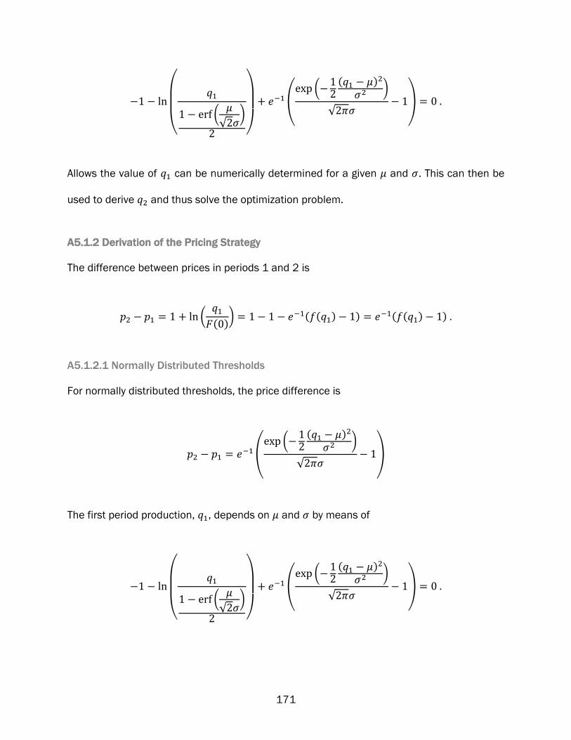
171

(

(

√ )

)

( (

( )

)

√ )

Allows the value of can be numerically determined for a given and . This can then be

used to derive and thus solve the optimization problem.


The difference between prices in periods 1 and 2 is

(

( )) ( ( ) ) ( ( ) )


For normally distributed thresholds, the price difference is

( (

( )

)

√ )

The first period production, , depends on and by means of

(

(

√ )

)

( (

( )

)

√ )

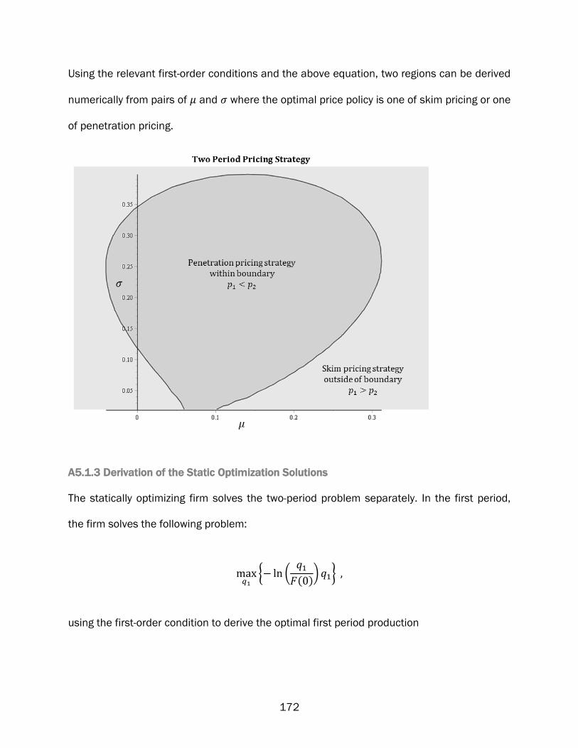
172

Using the relevant first-order conditions and the above equation, two regions can be derived

numerically from pairs of and where the optimal price policy is one of skim pricing or one

of penetration pricing.


The statically optimizing firm solves the two-period problem separately. In the first period,

the firm solves the following problem:

{ (

( )) }

using the first-order condition to derive the optimal first period production

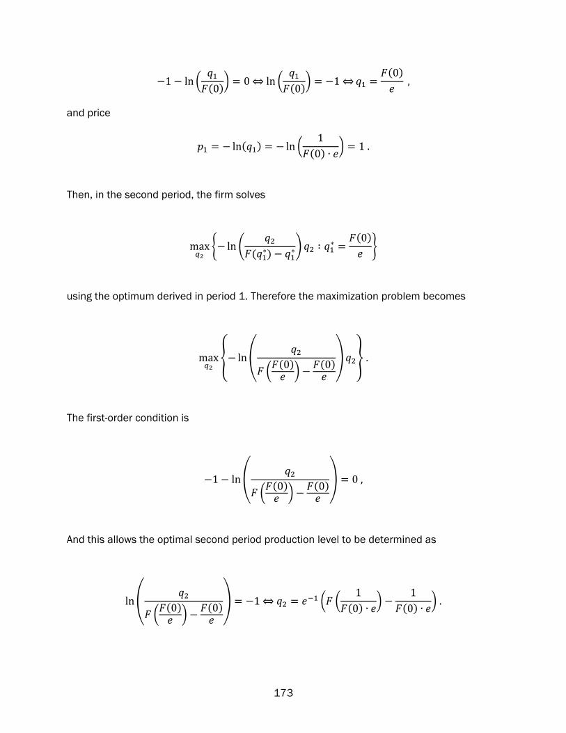
173

(

( ))

⇔ (

( ))

⇔

( )

and price

( ) (

( ) )

Then, in the second period, the firm solves

{ (

( )

)

( )

}

using the optimum derived in period 1. Therefore the maximization problem becomes

{ (

( ( ) )

( )

) }


(

( ( ) )

( )

)

And this allows the optimal second period production level to be determined as

(

( ( ) )

( )

)

⇔ ( (

( ) )

( ) )

174

The price in the second period is

(

( )

) ( ( (

( )

)

( ) )

(

( ) )

( )

)


The firm optimizing over eight periods solves the following maximization problem:

{

(

( ))

(

( ) )

(

( ) )

(

( ) )

(

( ) )

(

( ) )

(

( ) )

(

( ) )}

The first order conditions are:

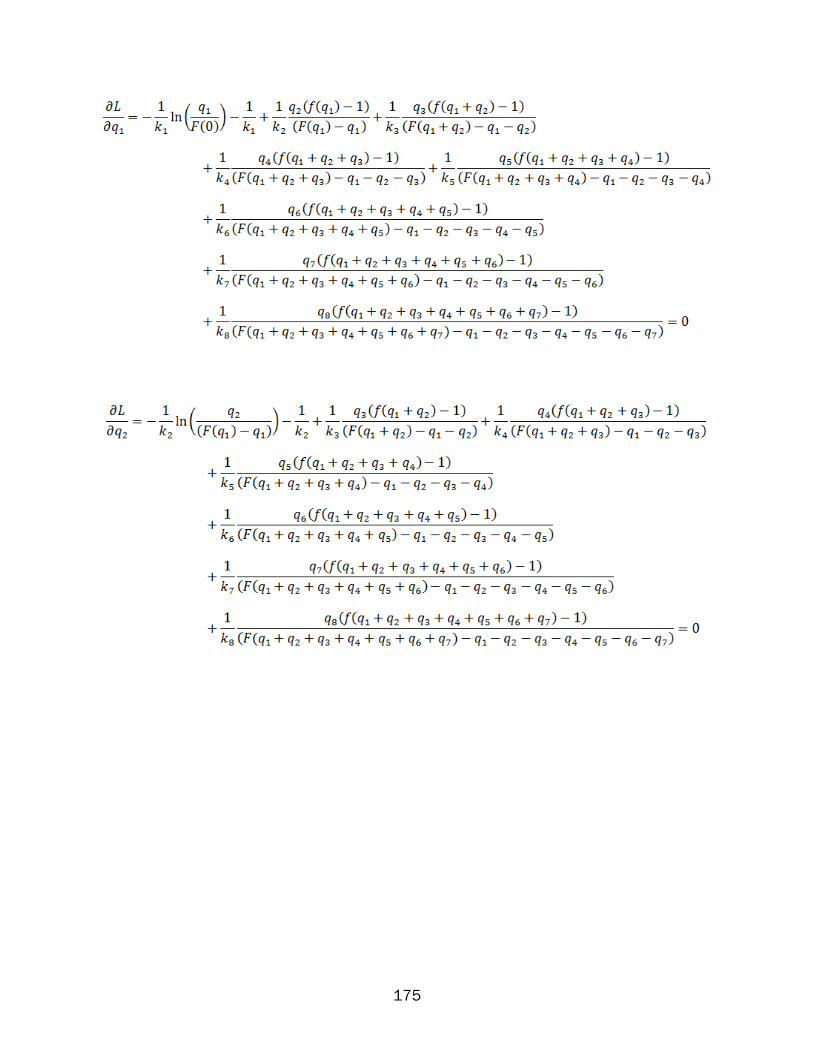
175

176

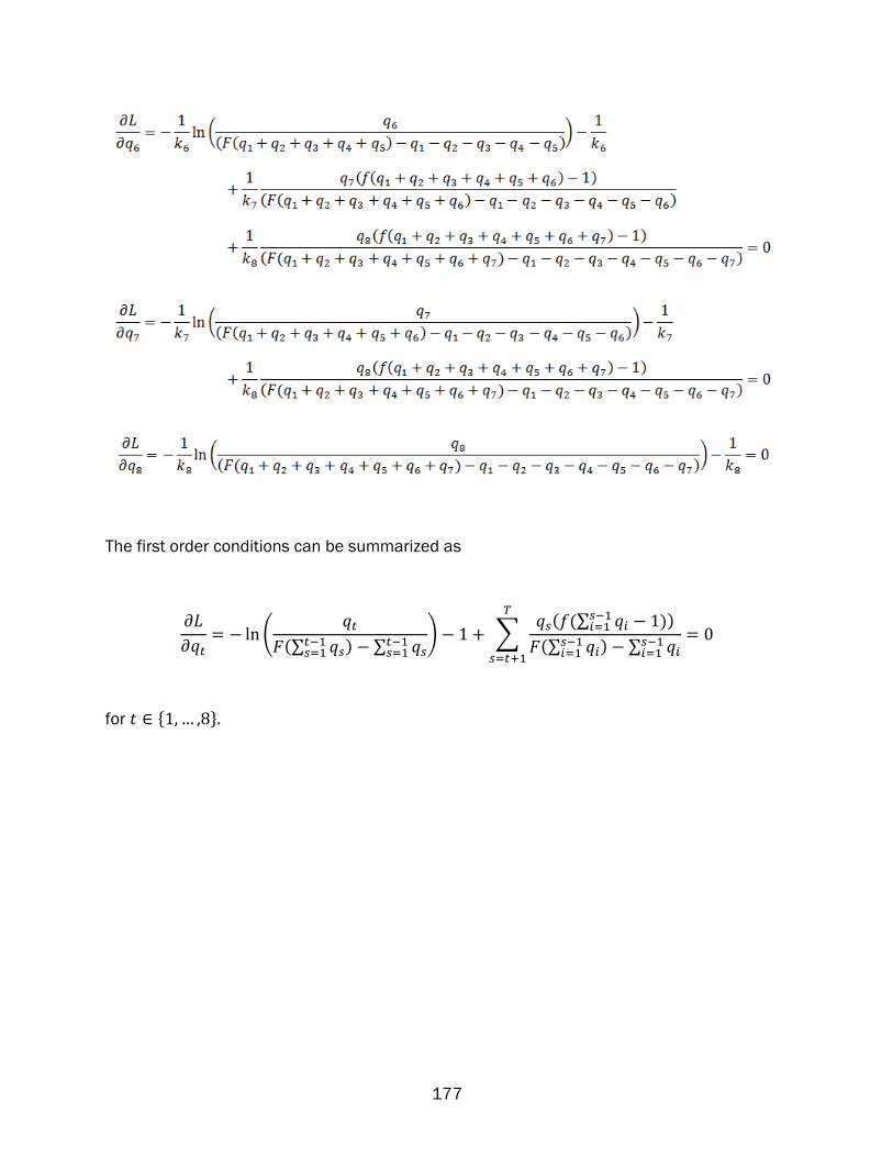
177

The first order conditions can be summarized as

(

(∑ ) ∑

) ∑ ( (∑

))

(∑ ) ∑

for

178

A5.2.1 Numeric Solutions for Various Distributions

( )

Period

Per period

production

Total

adoption

Per period

profit

Cumulative

profit Price

1 0.0917 0.0917 0.0503 0.0503 0.5484

2 0.0860 0.1777 0.0736 0.1239 0.8555

3 0.0869 0.2646 0.1010 0.2249 1.1627

4 0.0905 0.3551 0.1255 0.3504 1.3861

5 0.0957 0.4508 0.1429 0.4932 1.4931

6 0.1019 0.5527 0.1501 0.6433 1.4722

7 0.1094 0.6622 0.1441 0.7874 1.3171

8 0.1205 0.7826 0.1205 0.9079 1.0000

( )

Period Per period

production

Total

adoption

Per period

profit

Cumulative

profit Price

1 0.0664 0.0664 0.0211 0.0211 0.3173

2 0.0691 0.1355 0.0918 0.1128 1.3277

3 0.0823 0.2178 0.1558 0.2687 1.8932

4 0.1010 0.3188 0.1990 0.4676 1.9697

5 0.1101 0.4289 0.2004 0.6680 1.8199

6 0.1127 0.5417 0.1829 0.8509 1.6225

7 0.1167 0.6584 0.1597 1.0105 1.3679

8 0.1257 0.7841 0.1257 1.1362 1.0000

179

( )

Period Per period

production

Total

adoption

Per period

profit

Cumulative

profit Price

1 0.0963 0.0963 0.1196 0.1196 1.2416

2 0.0967 0.1930 0.1286 0.2481 1.3298

3 0.0970 0.2900 0.1368 0.3850 1.4111

4 0.0973 0.3872 0.1446 0.5295 1.4865

5 0.0975 0.4847 0.1518 0.6813 1.5567

6 0.0977 0.5824 0.1585 0.8398 1.6225

7 0.1063 0.6887 0.1455 0.9853 1.3679

8 0.1145 0.8032 0.1145 1.0998 1.0000

( )

Period Per period

production

Total

adoption

Per period

profit

Cumulative

profit Price

1 0.0986 0.0986 0.1781 0.1781 1.8057

2 0.0987 0.1973 0.1748 0.3529 1.7717

3 0.0987 0.2960 0.1714 0.5243 1.7365

4 0.0988 0.3948 0.1680 0.6923 1.7000

5 0.0989 0.4937 0.1643 0.8566 1.6620

6 0.0989 0.5926 0.1605 1.0172 1.6225

7 0.1037 0.6964 0.1419 1.1591 1.3679

8 0.1117 0.8081 0.1117 1.2708 1.0000

180


A5.3.1 Derivation of the Optimal Production and Price over T Periods

Assuming that ( ) , the firm’s -period maximization problem

is

{∑

(

(∑ ) ∑

)

}


In the homogeneous case, the firm solves the following maximization problem:

{∑ (

( ) )

}

which yields first-order conditions

(

(∑ ) ∑

) ∑ ( (∑

) )

(∑ ) ∑

181

Therefore production in period can be determined by

(

( ) ) ∑

( ( ) )

( )

⇔ (

( ) ) ∑

( ( ) )

( )

⇔

( ) ( ∑

( ( ) )

( )

)

⇔ ( ( ) ) ( ∑

( ( ) )

( )

)

The value of must be implicitly determined.

The optimal price can then be calculated using the optimal production levels by

∑ ( ( ) )

( )

∑ ( ( ) )

( )

∑ ( ( ) ) ( ∑ ( ( ) )

( )

)

182


When the adopter population is heterogeneous, the firm solves the maximization problem

{∑

(

(∑ ) ∑

)

}

by using the set of first order conditions:

(

(∑ ) ∑

)

∑

( (∑ ) )

( (∑ ) ∑

)

Using the definition that ∑ , this expression can also be written as

(

( ) )

∑

( ( ) )

( ( ) )

Production can be determined by solving

(

( ) ) ∑

( ( ) )

( ( ) )

⇔ (

( ) ) ∑

( ( ) )

( ( ) )

⇔

( ) ( ∑

( ( ) )

( ( ) )

)

183

⇔ ( ( ) ) ( ∑

( ( ) )

( ( ) )

)

Because the sum in the right hand side depends on its value must be determined

implicitly.

Price in period can be determined from the first order conditions to be

∑

( ( ) )

( ( ) )

( ∑

( ( ) )

( ( ) )

)


If thresholds are normally distributed, the CDF and PDF of thresholds, respectively, are

( )

(( )

√ )

( )

( )

( ( )

)

√

Where the error function, ( ) is defined as is conventional: ( )

√ ∫

Therefore production is determined by

(

(( )

√ )

)

(

∑

( (

( )

)

√ )

(( )

√ )

)

184

and price is determined by

∑

( (

( )

)

√ )

(( )

√ )

A5.3.1.4 Uniformly Distributed Thresholds

The PDF and CDF of the uniform distribution are as follows:

( ) {

( )

( ) {

If then no thresholds are crossed. In this case there can be no adoption. We

therefore assume that , which is equivalent to the assumption that

( )

When , optimal production and price are

(

) ( ∑

(

)

)

and

∑ (

)

185

When , optimal production and price are

( ) ( ∑

)

and

∑

The inequality could be first met in any of the periods, or it could never be met.

This means that there are a total of possible solutions to consider, which may or may

not be consistent with the distribution of thresholds.

There are two cases describing the penetration through the market:

adoption may permeates the entire market as the length of the planning period

increases, or

we may have a fixed point, expressed by the relation ( )

after which

adoption cannot continue.



The difference in price period-over-period in the homogeneous case is

∑ ( ( ) )

( )

∑ ( ( ) )

( )

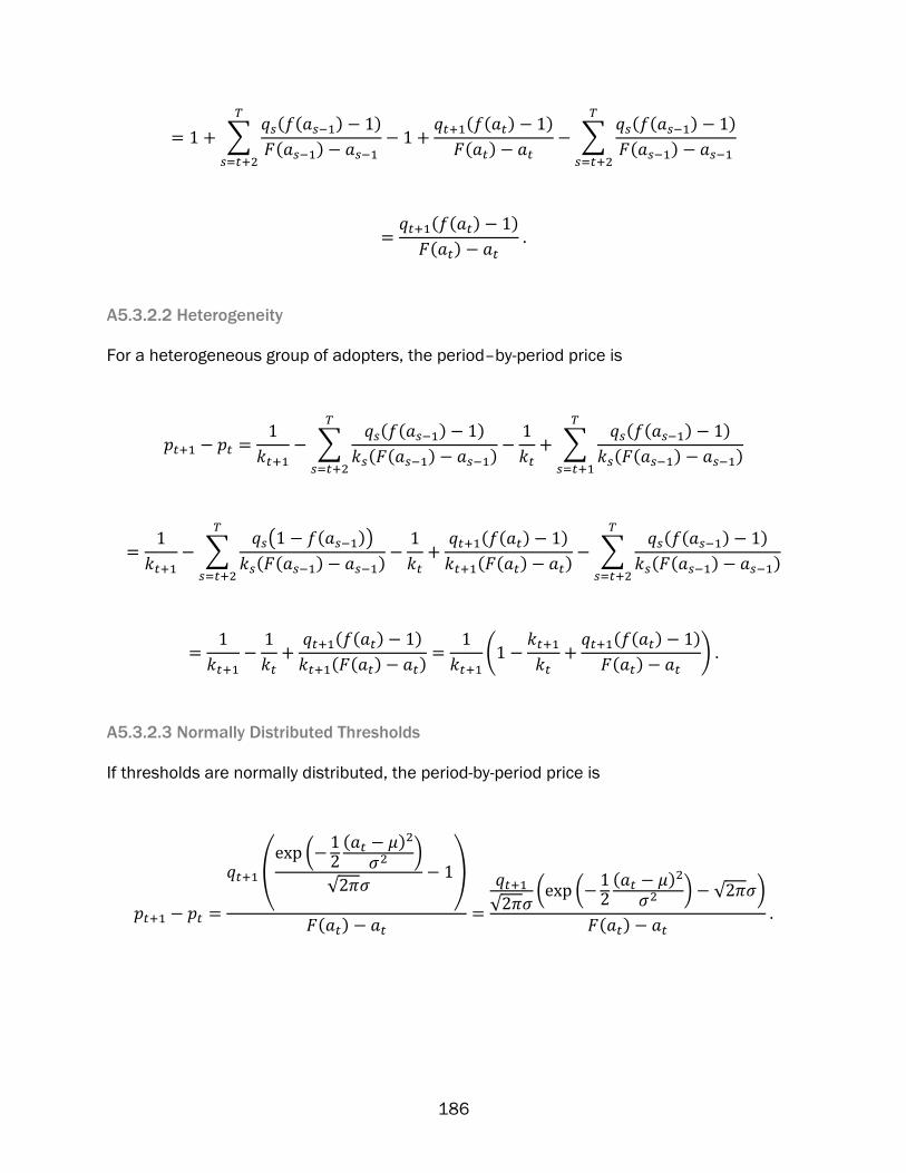
186

∑ ( ( ) )

( )

( ( ) )

( ) ∑

( ( ) )

( )

( ( ) )

( )


For a heterogeneous group of adopters, the period–by-period price is

∑

( ( ) )

( ( ) )

∑

( ( ) )

( ( ) )

∑

( ( ))

( ( ) )

( ( ) )

( ( ) ) ∑

( ( ) )

( ( ) )

( ( ) )

( ( ) )

(

( ( ) )

( ) )


If thresholds are normally distributed, the period-by-period price is

( (

( )

)

√ )

( )

√ ( (

( )

) √ )

( )

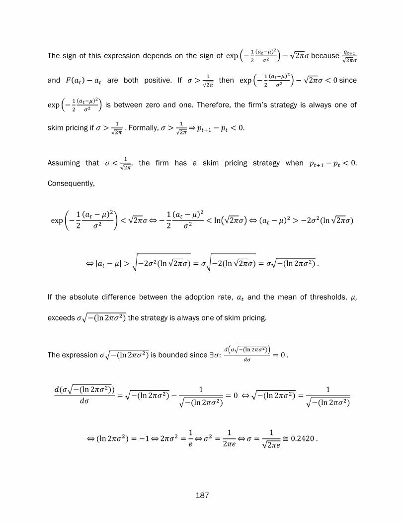
187

The sign of this expression depends on the sign of (

( )

) √ because

√

and ( ) are both positive. If

√ then (

( )

) √ since

(

( )

) is between zero and one. Therefore, the firm’s strategy is always one of

skim pricing if

√ Formally,

√

⇒

Assuming that

√ , the firm has a skim pricing strategy when

Consequently,

(

( )

) √

⇔

( )

(√ )

⇔ ( ) ( √ )

⇔| | √ ( √ ) √ ( √ ) √ ( )

If the absolute difference between the adoption rate, and the mean of thresholds,

exceeds √ ( ) the strategy is always one of skim pricing.

The expression √ ( ) is bounded since ( √ ( ))

( √ ( ))

√ ( )

√ ( )

⇔ √ ( )

√ ( )

⇔( )

⇔

⇔

⇔

√

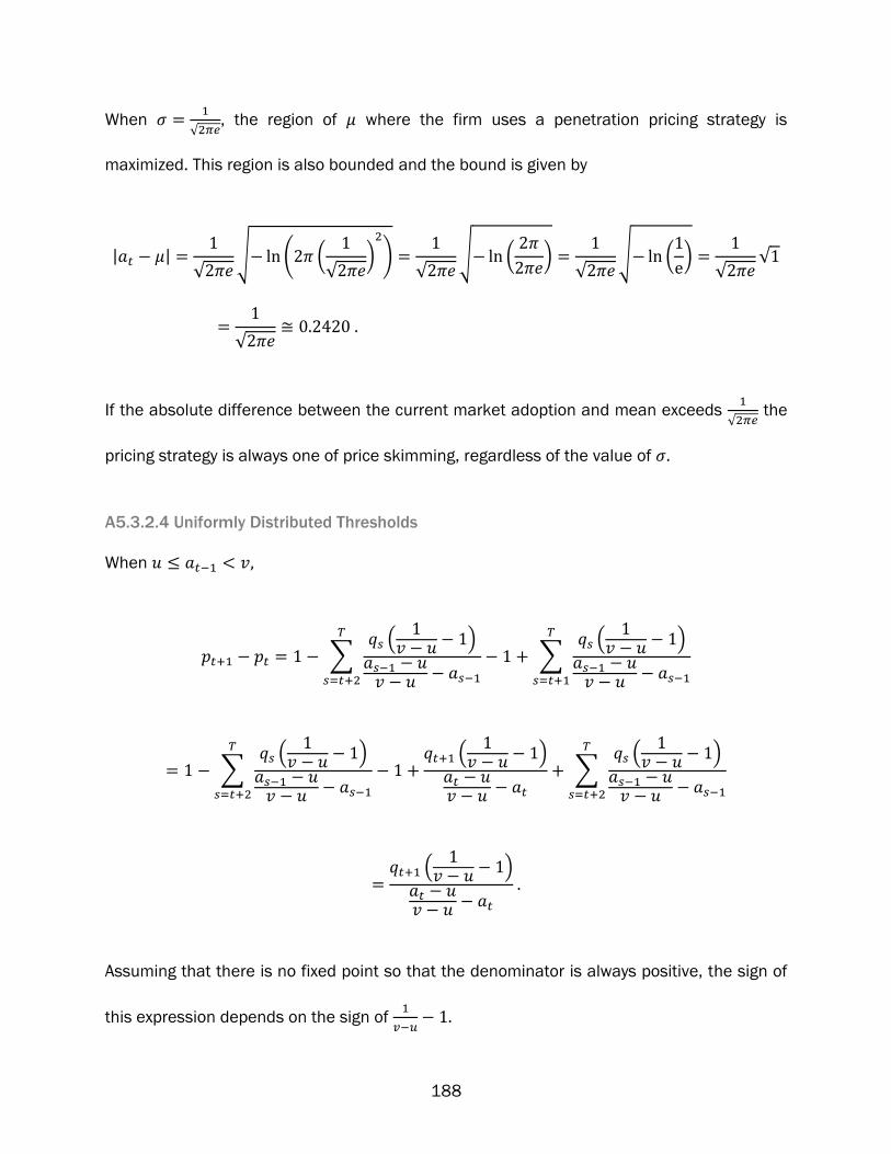
188

When

√ , the region of where the firm uses a penetration pricing strategy is

maximized. This region is also bounded and the bound is given by

| |

√ √ ( (

√ )

)

√ √ (

)

√ √ (

)

√ √

√

If the absolute difference between the current market adoption and mean exceeds

√ the

pricing strategy is always one of price skimming, regardless of the value of

A5.3.2.4 Uniformly Distributed Thresholds

When

∑ (

)

∑ (

)

∑ (

)

(

)

∑ (

)

(

)

Assuming that there is no fixed point so that the denominator is always positive, the sign of

this expression depends on the sign of

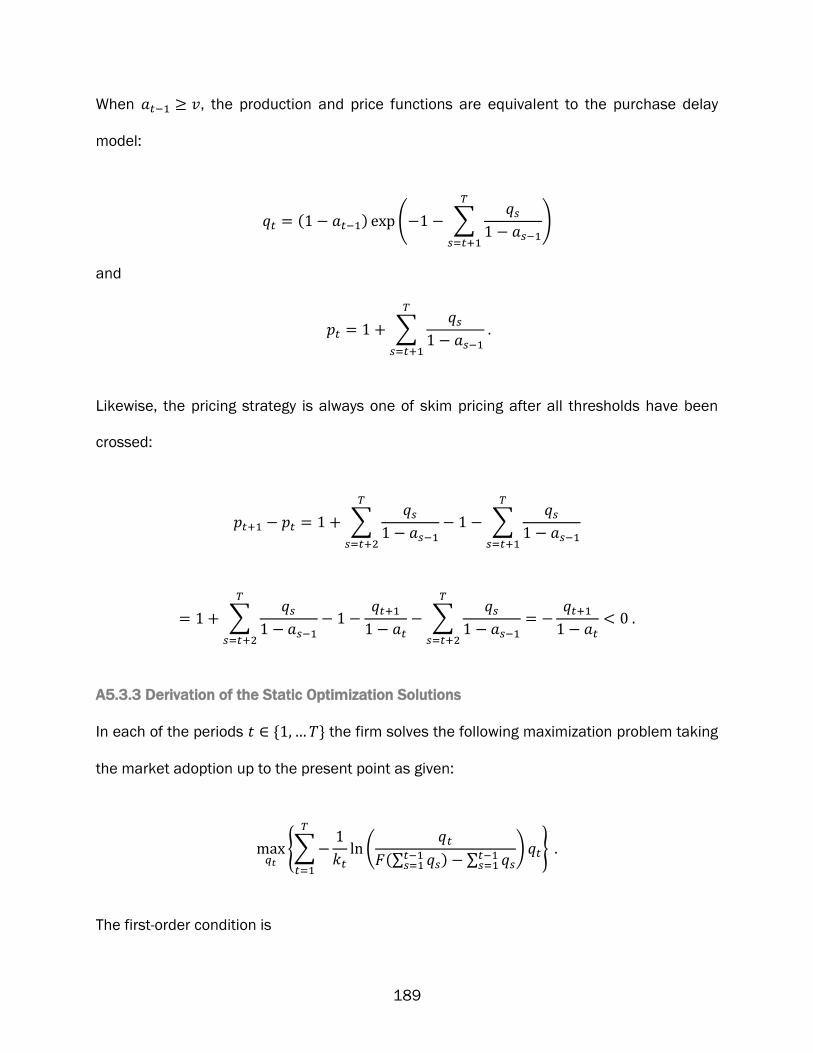
189

When , the production and price functions are equivalent to the purchase delay

model:

( ) ( ∑

)

and

∑

Likewise, the pricing strategy is always one of skim pricing after all thresholds have been

crossed:

∑

∑

∑

∑


In each of the periods the firm solves the following maximization problem taking

the market adoption up to the present point as given:

{∑

(

(∑ ) ∑

)

}


190

(

(∑ ) ∑

)

(

(∑ ) ∑

)

⇔

(∑ ) ∑

⇔

(∑

) ∑

Production does not depend on the heterogeneity parameters,


(

(∑ ) ∑

)

Because , any amount of heterogeneity will cause the price path to decrease

through time.

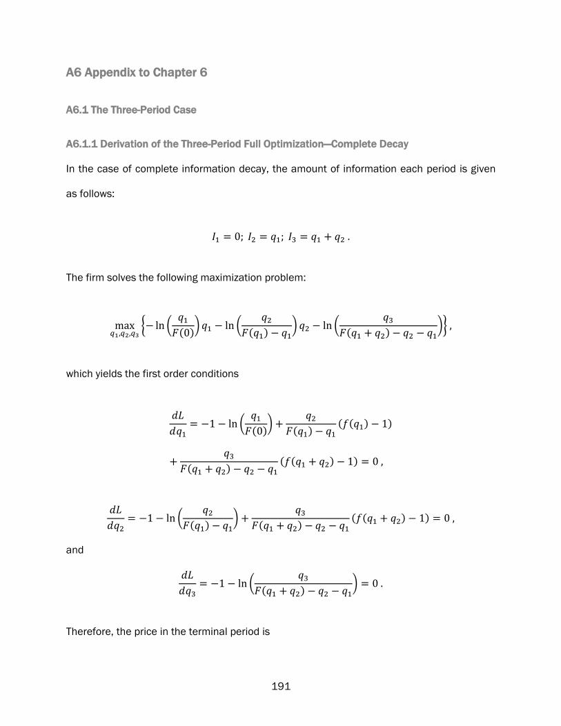
191


A6.1 The Three-Period Case

A6.1.1 Derivation of the Three-Period Full Optimization—Complete Decay

In the case of complete information decay, the amount of information each period is given

as follows:

The firm solves the following maximization problem:

{ (

( )) (

( ) ) (

( ) )}

which yields the first order conditions

(

( ))

( )

( ( ) )

( )

( ( ) )

(

( ) )

( )

( ( ) )

and

(

( ) )

Therefore, the price in the terminal period is

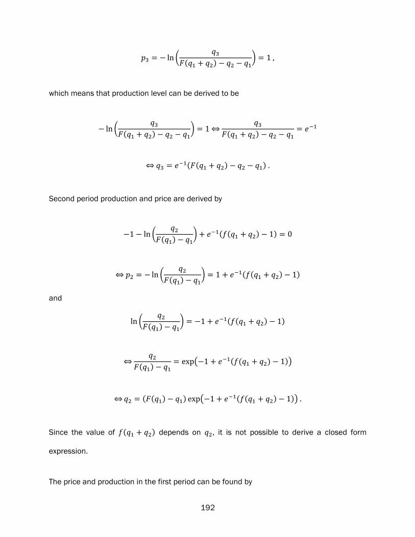
192

(

( ) )

which means that production level can be derived to be

(

( ) )

⇔

( )

⇔ ( ( ) )

Second period production and price are derived by

(

( ) ) ( ( ) )

⇔ (

( ) ) ( ( ) )

and

(

( ) ) ( ( ) )

⇔

( ) ( ( ( ) ))

⇔ ( ( ) ) ( ( ( ) ))

Since the value of ( ) depends on , it is not possible to derive a closed form

expression.

The price and production in the first period can be found by

193

(

( ))

( )

( ( ) )

( )

( ( ) )

⇔ (

( ))

⇔

( )

( ( ) )

( )

( ( ) )

and

(

( )) ( ( ( ) ))( ( ) ) ( ( ) )

⇔ ( ) ( ( ( ( ) ))( ( ) )

( ( ) ))

Again, the value of must be implicitly determined once is known.

A6.1.2 Derivation of the Three-Period Full Optimization—No Decay

If there is no information decay, the amount of information in each period is

The firm therefore solves the following maximization problem:

{ (

( )) (

( ) ) (

( ) )}

The first-order conditions are

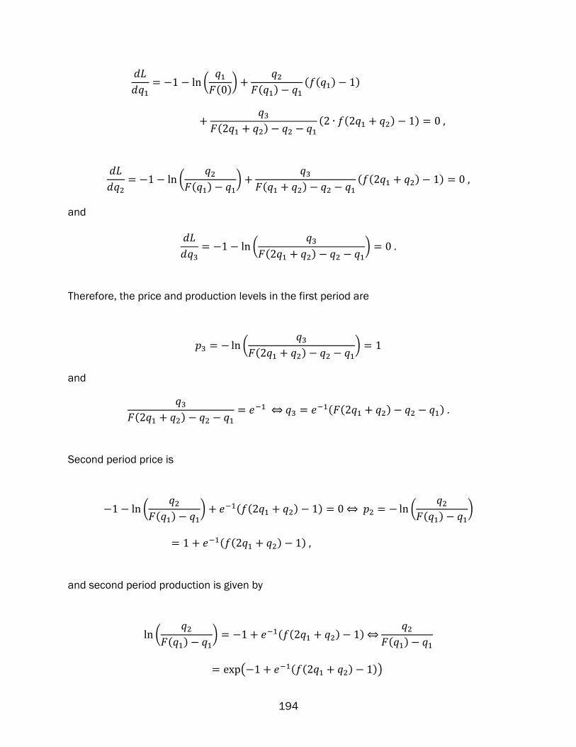
194

(

( ))

( )

( ( ) )

( )

( ( ) )

(

( ) )

( )

( ( ) )

and

(

( ) )

Therefore, the price and production levels in the first period are

(

( ) )

and

( )

⇔ ( ( ) )

Second period price is

(

( ) ) ( ( ) )

⇔ (

( ) )

( ( ) )

and second period production is given by

(

( ) ) ( ( ) )

⇔

( )

( ( ( ) ))

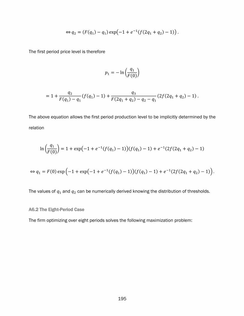
195

⇔ ( ( ) ) ( ( ( ) ))

The first period price level is therefore

(

( ))

( )

( ( ) )

( )

( ( ) )

The above equation allows the first period production level to be implicitly determined by the

relation

(

( )) ( ( ( ) ))( ( ) ) ( ( ) )

⇔ ( ) ( ( ( ( ) ))( ( ) ) ( ( ) ))

The values of and can be numerically derived knowing the distribution of thresholds.


The firm optimizing over eight periods solves the following maximization problem:

196

{

(

( ))

(

( ) )

(

( ) )

(

( ) )

(

( ) )

(

( ) )

(

( ) )

(

( ) )}

The first-order conditions can be summarized as

(

(∑ ( ) ) ∑

)

∑

( ) ( (∑ ( ) ) )

( (∑ ( ) ) ∑

)

for

Explicitly, the first-order conditions are:

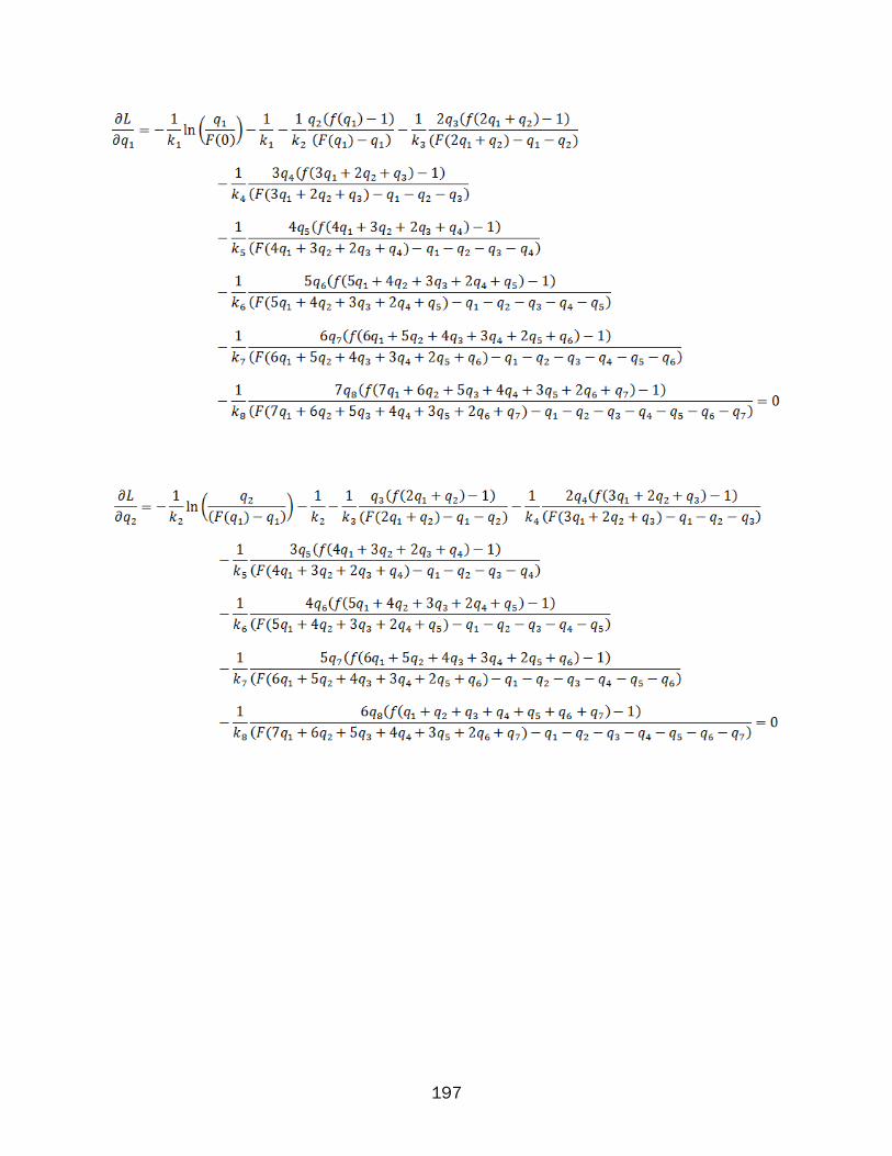
197

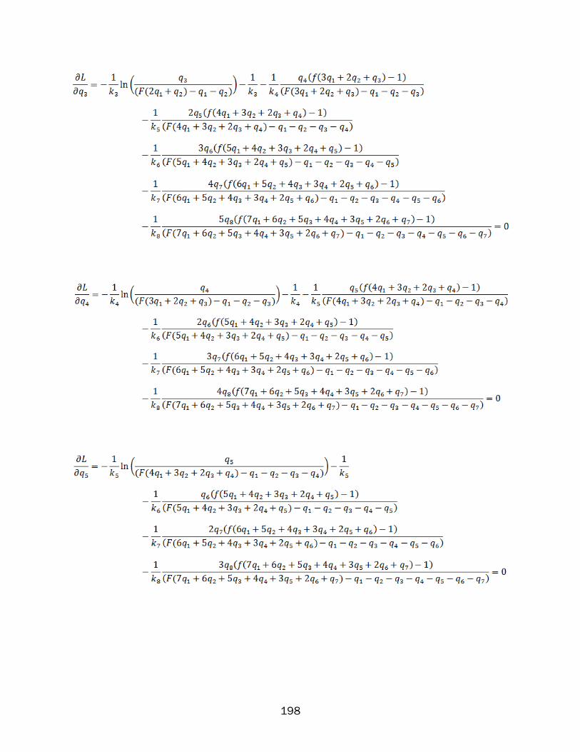
198

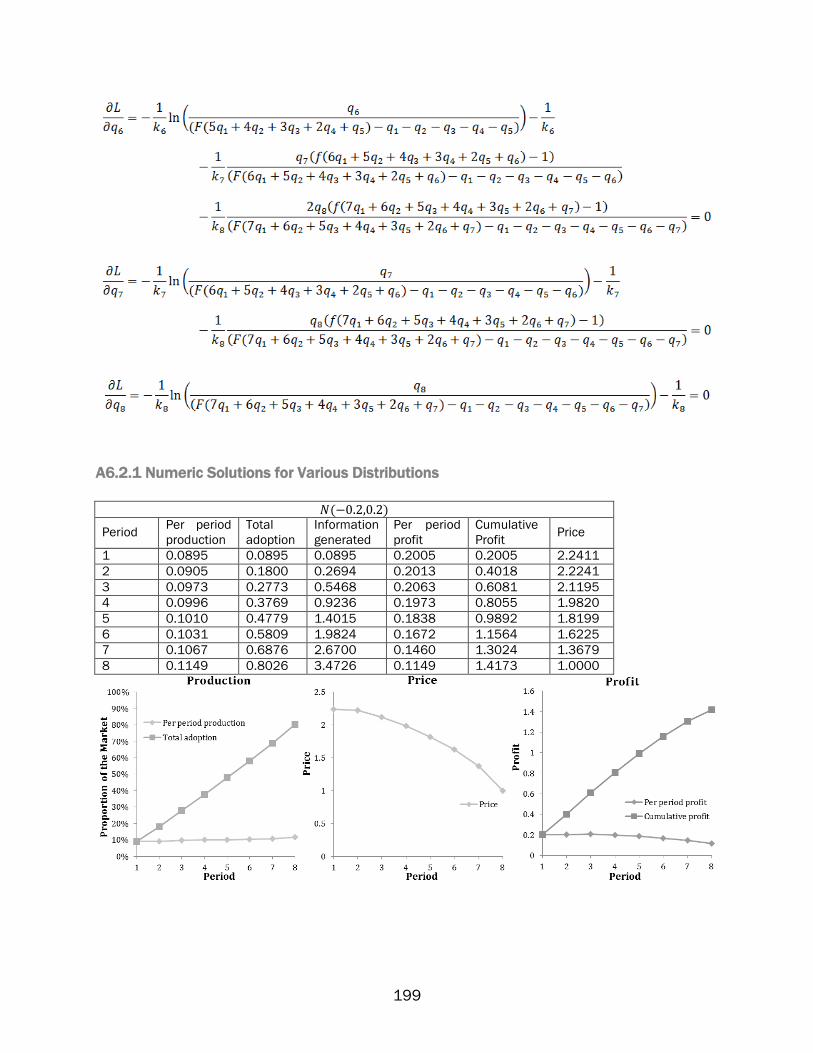
199

A6.2.1 Numeric Solutions for Various Distributions

( )

Period Per period

production

Total

adoption

Information

generated

Per period

profit

Cumulative

Profit Price

1 0.0895 0.0895 0.0895 0.2005 0.2005 2.2411

2 0.0905 0.1800 0.2694 0.2013 0.4018 2.2241

3 0.0973 0.2773 0.5468 0.2063 0.6081 2.1195

4 0.0996 0.3769 0.9236 0.1973 0.8055 1.9820

5 0.1010 0.4779 1.4015 0.1838 0.9892 1.8199

6 0.1031 0.5809 1.9824 0.1672 1.1564 1.6225

7 0.1067 0.6876 2.6700 0.1460 1.3024 1.3679

8 0.1149 0.8026 3.4726 0.1149 1.4173 1.0000

200

( )

Period Per period

production

Total

adoption

Information

generated

Per period

profit

Cumulative

Profit Price

1 0.0798 0.0798 0.0798 0.1464 0.1464 1.8355

2 0.0717 0.1515 0.2312 0.1493 0.2957 2.0825

3 0.0885 0.2400 0.4712 0.1861 0.4818 2.1025

4 0.1035 0.3434 0.8146 0.2051 0.6869 1.9819

5 0.1064 0.4498 1.2645 0.1936 0.8805 1.8199

6 0.1086 0.5584 1.8229 0.1762 1.0567 1.6225

7 0.1124 0.6709 2.4938 0.1538 1.2105 1.3679

8 0.1211 0.7920 3.2857 0.1211 1.3316 1.0000

( )

Period Per period

production

Total

adoption

Information

generated

Per period

profit

Cumulative

Profit Price

1 0.0733 0.0733 0.0733 0.0566 0.0566 0.7717

2 0.0439 0.1172 0.1906 0.0643 0.1209 1.4649

3 0.0569 0.1741 0.3647 0.1056 0.2265 1.8556

4 0.0884 0.2626 0.6273 0.1723 0.3988 1.9487

5 0.1169 0.3794 1.0067 0.2127 0.6115 1.8198

6 0.1225 0.5019 1.5086 0.1988 0.8102 1.6225

7 0.1268 0.6288 2.1373 0.1735 0.9837 1.3679

8 0.1366 0.7653 2.9027 0.1366 1.1203 1.0000

201

A6.2.2 Numeric Solutions for Various Rates of Information Decay

( )

Period

Per period

production

Total

adoption Information Profit Price

1 0.0733 0.0733 0.0733 0.0566 0.7717

2 0.0439 0.1172 0.1906 0.0643 1.4649

3 0.0569 0.1741 0.3647 0.1056 1.8556

4 0.0884 0.2626 0.6273 0.1723 1.9487

5 0.1169 0.3794 1.0067 0.2127 1.8198

6 0.1225 0.5019 1.5086 0.1988 1.6225

7 0.1268 0.6288 2.1373 0.1735 1.3679

8 0.1366 0.7653 2.9027 0.1366 1.0000

Period Per period

production

Total


1 0.0784 0.0784 0 0.0553 0.7045

2 0.0516 0.1300 0.0784 0.0681 1.3199

3 0.0618 0.1918 0.1889 0.1067 1.7284

4 0.0843 0.2761 0.3335 0.1590 1.8866

5 0.1096 0.3857 0.5262 0.1988 1.8140

6 0.1209 0.5066 0.7803 0.1962 1.6225

7 0.1256 0.6322 1.0918 0.1719 1.3679

8 0.1353 0.7675 1.4511 0.1353 1.0000

Period Per period

production

Total


1 0.0836 0.0836 0 0.0536 0.6408

2 0.0617 0.1453 0.0836 0.0715 1.1599

3 0.0692 0.2145 0.1871 0.1079 1.5588

4 0.0837 0.2981 0.3080 0.1480 1.7694

5 0.1015 0.3996 0.4521 0.1800 1.7740

6 0.1157 0.5153 0.6257 0.1872 1.6188

7 0.1232 0.6385 0.8281 0.1686 1.3678

8 0.1330 0.7715 1.0526 0.1330 1.0000

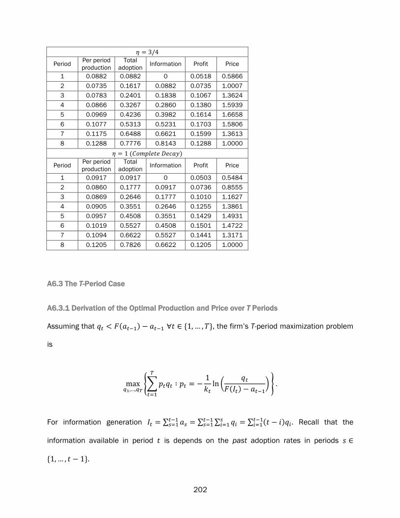
202

Period Per period

production

Total


1 0.0882 0.0882 0 0.0518 0.5866

2 0.0735 0.1617 0.0882 0.0735 1.0007

3 0.0783 0.2401 0.1838 0.1067 1.3624

4 0.0866 0.3267 0.2860 0.1380 1.5939

5 0.0969 0.4236 0.3982 0.1614 1.6658

6 0.1077 0.5313 0.5231 0.1703 1.5806

7 0.1175 0.6488 0.6621 0.1599 1.3613

8 0.1288 0.7776 0.8143 0.1288 1.0000

( )

Period Per period

production

Total


1 0.0917 0.0917 0 0.0503 0.5484

2 0.0860 0.1777 0.0917 0.0736 0.8555

3 0.0869 0.2646 0.1777 0.1010 1.1627

4 0.0905 0.3551 0.2646 0.1255 1.3861

5 0.0957 0.4508 0.3551 0.1429 1.4931

6 0.1019 0.5527 0.4508 0.1501 1.4722

7 0.1094 0.6622 0.5527 0.1441 1.3171

8 0.1205 0.7826 0.6622 0.1205 1.0000


A6.3.1 Derivation of the Optimal Production and Price over T Periods

Assuming that ( ) , the firm’s T-period maximization problem

is

{∑

(

( )

)

}

For information generation ∑ ∑ ∑

∑ ( )

. Recall that the

information available in period is depends on the past adoption rates in periods

.

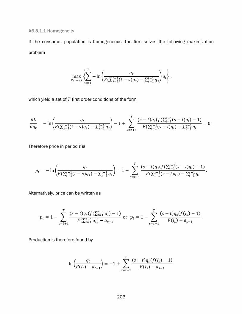
203


If the consumer population is homogeneous, the firm solves the following maximization

problem

{∑ (

(∑ ( ) ) ∑

)

}

which yield a set of first order conditions of the form

(

(∑ ( ) ) ∑

) ∑( ) ( (∑ ( )

) )

(∑ ( ) ) ∑

Therefore price in period is

(

(∑ ( ) ) ∑

) ∑( ) ( (∑ ( )

) )

(∑ ( ) ) ∑

Alternatively, price can be written as

∑( ) ( (∑

) )

(∑ )

∑( ) ( ( ) )

( )

Production is therefore found by

(

( ) ) ∑

( ) ( ( ) )

( )

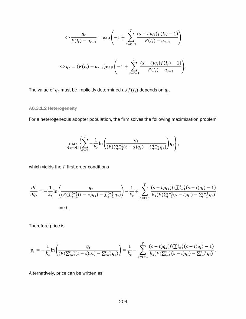
204

⇔

( ) ( ∑

( ) ( ( ) )

( )

)

⇔ ( ( ) ) ( ∑

( ) ( ( ) )

( )

)

The value of must be implicitly determined as ( ) depends on


For a heterogeneous adopter population, the firm solves the following maximization problem

{∑

(

( (∑ ( )

) ∑

)

)

}

which yields the first order conditions

(

( (∑ ( ) ) ∑

)

)

∑

( ) ( (∑ ( ) ) )

( (∑ ( ) ) ∑

)

Therefore price is

(

( (∑ ( ) ) ∑

)

)

∑

( ) ( (∑ ( ) ) )

( (∑ ( ) ) ∑

)

Alternatively, price can be written as

205

∑

( ) ( (∑ ) )

( (∑ ) )

∑

( ) ( ( ) )

( ( ) )

Production is therefore determined by

(

( ) ) ∑

( ) ( ( ) )

( ( ) )

⇔

( ) ( ∑

( ) ( ( ) )

( ( ) )

)

⇔ ( ( ) ) ( ∑

( ) ( ( ) )

( ( ) )

)

The value of must be implicitly determined as ( ) depends on

A6.3.2 Derivation of the Price Strategy


If the consumer population is homogeneous, the difference between prices in successive

periods is

∑( ) ( ( ) )

( )

∑( ) ( ( ) )

( )

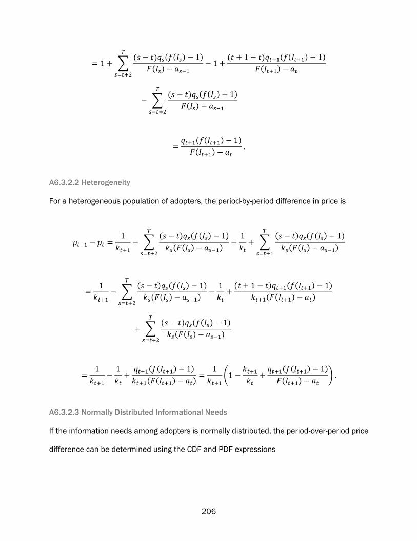
206

∑( ) ( ( ) )

( )

( ) ( ( ) )

( )

∑( ) ( ( ) )

( )

( ( ) )

( )


For a heterogeneous population of adopters, the period-by-period difference in price is

∑

( ) ( ( ) )

( ( ) )

∑

( ) ( ( ) )

( ( ) )

∑

( ) ( ( ) )

( ( ) )

( ) ( ( ) )

( ( ) )

∑( ) ( ( ) )

( ( ) )

( ( ) )

( ( ) )

(

( ( ) )

( ) )

A6.3.2.3 Normally Distributed Informational Needs

If the information needs among adopters is normally distributed, the period-over-period price

difference can be determined using the CDF and PDF expressions

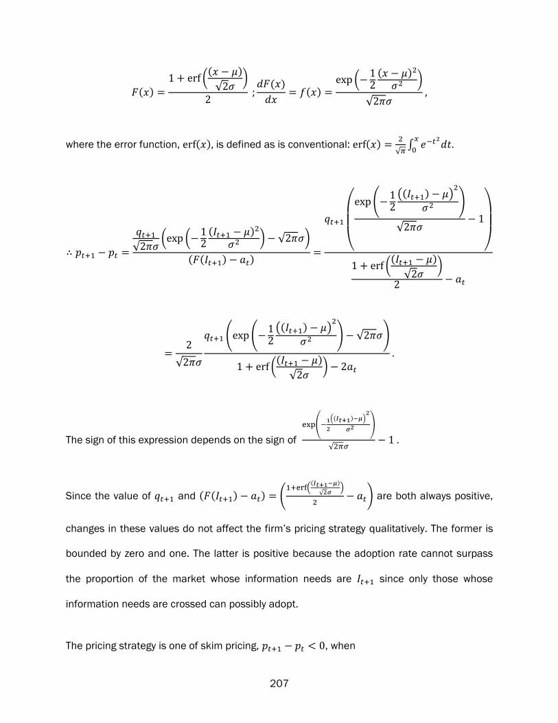
207

( )

(( )

√ )

( )

( )

( ( )

)

√

where the error function, ( ) is defined as is conventional: ( )

√ ∫

√ ( (

( )

) √ )

( ( ) )

(

(

(( ) )

)

√

)

(( )

√ )

√

( ( (( ) )

) √ )

(( )

√ )

The sign of this expression depends on the sign of

(

(( ) )

)

√

Since the value of and ( ( ) ) ( (

( )

√ )

) are both always positive,

changes in these values do not affect the firm’s pricing strategy qualitatively. The former is

bounded by zero and one. The latter is positive because the adoption rate cannot surpass

the proportion of the market whose information needs are since only those whose

information needs are crossed can possibly adopt.

The pricing strategy is one of skim pricing, , when

208

(

( )

) √

The expression

( )

is always positive which means that (

( )

)

Therefore, if

√ then √ , which means that (

( )

) √ for

any value of and

Skim pricing is also always the dominant strategy for certain values of

(

( )

) √

⇔ (

( )

) √

⇔

( )

√

( ) √

⇔| | √ √

⇔| | √

Since depends on , the specific bounds for and in the above equation can only be

determined knowing the length of the planning period.

The expression has an absolute bound for certain values of | | because

( √ ( ))

The right-hand side achieves a minimum when

( √ ( ))

√ ( )

√ ( )

Therefore the bound can be derived by

209

√ ( )

√ ( )

⇔ ( )

⇔

⇔

⇔

√

Therefore when | |

√ the strategy is always one of price skimming.


In each period, the firm solves the following optimization problem

{∑

(

(∑ ∑

) ∑

)

}

using the first order condition

(

(∑ ∑

) ∑

)

Therefore production can be derived to be

(

( (∑ ∑

) ∑

)

)

⇔

( (∑ ∑

) ∑

)

⇔

( (∑ ∑

) ∑

)

( (∑ ) )

( ( ) )

.

Price is therefore

(

(∑ ∑

) ∑

)

Optimal Intertemporal Pricing ... - curve. · PDF fileThe firm does better by pricing a straightforward new product at a lower introductory price when the product is quite visible

Documents